

Compact Muon Solenoid
LHC, CERN
| CMS-TOP-22-006 ; CERN-EP-2023-124 | ||
| Search for physics beyond the standard model in top quark production with additional leptons in the context of effective field theory | ||
| CMS Collaboration | ||
| 28 July 2023 | ||
| JHEP 12 (2023) 068 | ||
| Abstract: A search for new physics in top quark production with additional final-state leptons is performed using data collected by the CMS experiment in proton-proton collisions at $ \sqrt{s}= $ 13 TeV at the LHC during 2016-2018. The data set corresponds to an integrated luminosity of 138 fb$ ^{-1} $. Using the framework of effective field theory (EFT), potential new physics effects are parametrized in terms of 26 dimension-six EFT operators. The impacts of EFT operators are incorporated through the event-level reweighting of Monte Carlo simulations, which allows for detector-level predictions. The events are divided into several categories based on lepton multiplicity, total lepton charge, jet multiplicity, and b-tagged jet multiplicity. Kinematic variables corresponding to the transverse momentum ($ p_{\mathrm{T}} $) of the leading pair of leptons and/or jets as well as the $ p_{\mathrm{T}} $ of on-shell Z bosons are used to extract the 95% confidence intervals of the 26 Wilson coefficients corresponding to these EFT operators. No significant deviation with respect to the standard model prediction is found. | ||
| Links: e-print arXiv:2307.15761 [hep-ex] (PDF) ; CDS record ; inSPIRE record ; HepData record ; Physics Briefing ; CADI line (restricted) ; | ||
| Figures & Tables | Summary | Additional Figures | References | CMS Publications |
|---|
| Figures | |

png pdf |
Figure 1:
Example Feynman diagrams illustrating Wilson coefficients from each of the categories listed in Table 1. From left to right, the diagrams show vertices associated with the $c_{\mathrm{tG}}$, $c_{\mathrm{t\ell}}^{(\ell)}$, $c_{\mathrm{Qq}}^{11}$, and $c_{\mathrm{Qt}}^{1}$. |

png pdf |
Figure 1-a:
Example Feynman diagrams illustrating Wilson coefficients from each of the categories listed in Table 1. From left to right, the diagrams show vertices associated with the $c_{\mathrm{tG}}$, $c_{\mathrm{t\ell}}^{(\ell)}$, $c_{\mathrm{Qq}}^{11}$, and $c_{\mathrm{Qt}}^{1}$. |

png pdf |
Figure 1-b:
Example Feynman diagrams illustrating Wilson coefficients from each of the categories listed in Table 1. From left to right, the diagrams show vertices associated with the $c_{\mathrm{tG}}$, $c_{\mathrm{t\ell}}^{(\ell)}$, $c_{\mathrm{Qq}}^{11}$, and $c_{\mathrm{Qt}}^{1}$. |

png pdf |
Figure 1-c:
Example Feynman diagrams illustrating Wilson coefficients from each of the categories listed in Table 1. From left to right, the diagrams show vertices associated with the $c_{\mathrm{tG}}$, $c_{\mathrm{t\ell}}^{(\ell)}$, $c_{\mathrm{Qq}}^{11}$, and $c_{\mathrm{Qt}}^{1}$. |

png pdf |
Figure 1-d:
Example Feynman diagrams illustrating Wilson coefficients from each of the categories listed in Table 1. From left to right, the diagrams show vertices associated with the $c_{\mathrm{tG}}$, $c_{\mathrm{t\ell}}^{(\ell)}$, $c_{\mathrm{Qq}}^{11}$, and $c_{\mathrm{Qt}}^{1}$. |
png pdf |
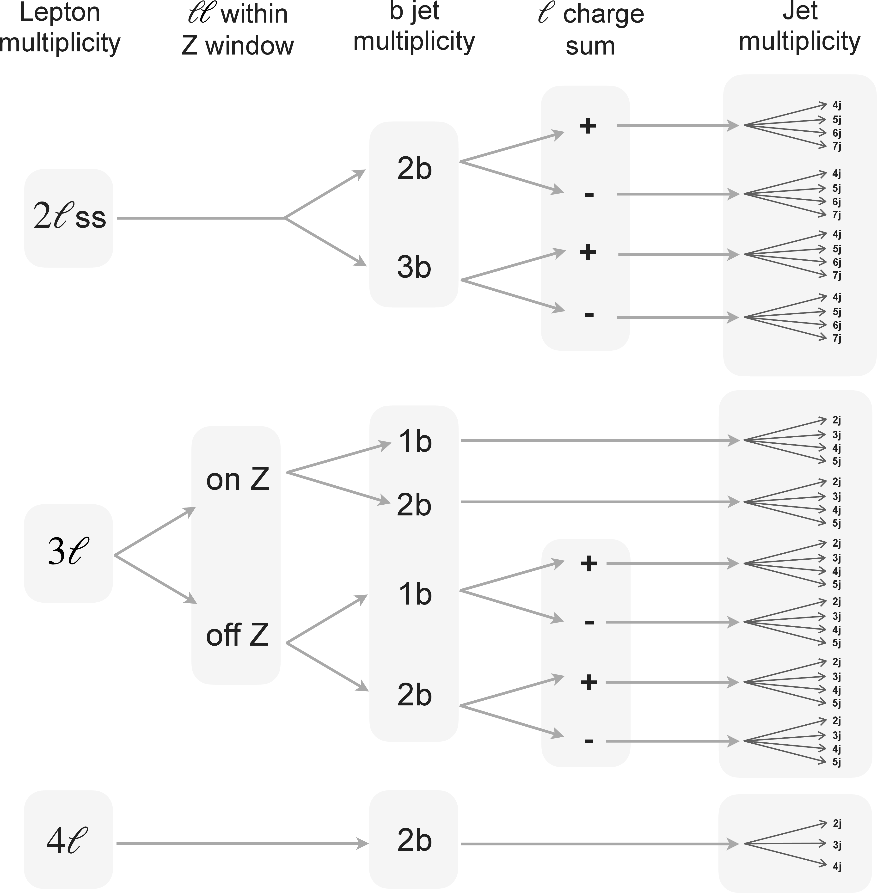
Figure 2:
Summary of the event selection categorization. The details for the selection requirements are described in Sections 5.1-5.3. |

png pdf |
Figure 3:
Example Feynman diagram illustrating how the $c_{\mathrm{Qq}}^{31}$ and $c_{\mathrm{Qq}}^{38}$ WCs can impact the processes in 3 $ \ell $ categories with two b quarks and an on-shell Z boson. These two WCs are a part of the $ \textrm{2hq2lq} $ group, but unlike the other WCs in this group, these two WCs are associated with operators that have vertices involving a top and bottom quark pair, as pictured in the figure. |

png pdf |
Figure 4:
The categories shown in these plots are 2 $ \ell\text{ss }2\mathrm{b} $ and 2 $ \ell\text{ss }3\mathrm{b} $. The prefit plots for each category are shown on the left side while the postfit plots are shown on the right side. The differential distribution in the plots is $ p_{\mathrm{T}}(\ell{\mathrm{j}} )_{\text{max}} $. The jet subcategories are arranged from low jet multiplicity to high jet multiplicity from left to right for each individual plot. For example, in the $2\ell\text{ss }2\mathrm{b} (+)$ plot, the first four bins are the $ p_{\mathrm{T}}(\ell{\mathrm{j}} )_{\text{max}} $ variable for $2\ell\text{ss }2\mathrm{b} (+) 4{\mathrm{j}} $, the next four bins are for $2\ell\text{ss }2\mathrm{b} (+) 5{\mathrm{j}} $, etc. The process labeled ``Conv.'' corresponds to the photon conversion background, ``Misid. leptons'' corresponds to misidentified leptons, and ``Charge misid.'' corresponds to leptons with a mismeasured charge. |

png pdf |
Figure 4-a:
The categories shown in these plots are 2 $ \ell\text{ss }2\mathrm{b} $ and 2 $ \ell\text{ss }3\mathrm{b} $. The prefit plots for each category are shown on the left side while the postfit plots are shown on the right side. The differential distribution in the plots is $ p_{\mathrm{T}}(\ell{\mathrm{j}} )_{\text{max}} $. The jet subcategories are arranged from low jet multiplicity to high jet multiplicity from left to right for each individual plot. For example, in the $2\ell\text{ss }2\mathrm{b} (+)$ plot, the first four bins are the $ p_{\mathrm{T}}(\ell{\mathrm{j}} )_{\text{max}} $ variable for $2\ell\text{ss }2\mathrm{b} (+) 4{\mathrm{j}} $, the next four bins are for $2\ell\text{ss }2\mathrm{b} (+) 5{\mathrm{j}} $, etc. The process labeled ``Conv.'' corresponds to the photon conversion background, ``Misid. leptons'' corresponds to misidentified leptons, and ``Charge misid.'' corresponds to leptons with a mismeasured charge. |

png pdf |
Figure 4-b:
The categories shown in these plots are 2 $ \ell\text{ss }2\mathrm{b} $ and 2 $ \ell\text{ss }3\mathrm{b} $. The prefit plots for each category are shown on the left side while the postfit plots are shown on the right side. The differential distribution in the plots is $ p_{\mathrm{T}}(\ell{\mathrm{j}} )_{\text{max}} $. The jet subcategories are arranged from low jet multiplicity to high jet multiplicity from left to right for each individual plot. For example, in the $2\ell\text{ss }2\mathrm{b} (+)$ plot, the first four bins are the $ p_{\mathrm{T}}(\ell{\mathrm{j}} )_{\text{max}} $ variable for $2\ell\text{ss }2\mathrm{b} (+) 4{\mathrm{j}} $, the next four bins are for $2\ell\text{ss }2\mathrm{b} (+) 5{\mathrm{j}} $, etc. The process labeled ``Conv.'' corresponds to the photon conversion background, ``Misid. leptons'' corresponds to misidentified leptons, and ``Charge misid.'' corresponds to leptons with a mismeasured charge. |

png pdf |
Figure 4-c:
The categories shown in these plots are 2 $ \ell\text{ss }2\mathrm{b} $ and 2 $ \ell\text{ss }3\mathrm{b} $. The prefit plots for each category are shown on the left side while the postfit plots are shown on the right side. The differential distribution in the plots is $ p_{\mathrm{T}}(\ell{\mathrm{j}} )_{\text{max}} $. The jet subcategories are arranged from low jet multiplicity to high jet multiplicity from left to right for each individual plot. For example, in the $2\ell\text{ss }2\mathrm{b} (+)$ plot, the first four bins are the $ p_{\mathrm{T}}(\ell{\mathrm{j}} )_{\text{max}} $ variable for $2\ell\text{ss }2\mathrm{b} (+) 4{\mathrm{j}} $, the next four bins are for $2\ell\text{ss }2\mathrm{b} (+) 5{\mathrm{j}} $, etc. The process labeled ``Conv.'' corresponds to the photon conversion background, ``Misid. leptons'' corresponds to misidentified leptons, and ``Charge misid.'' corresponds to leptons with a mismeasured charge. |

png pdf |
Figure 4-d:
The categories shown in these plots are 2 $ \ell\text{ss }2\mathrm{b} $ and 2 $ \ell\text{ss }3\mathrm{b} $. The prefit plots for each category are shown on the left side while the postfit plots are shown on the right side. The differential distribution in the plots is $ p_{\mathrm{T}}(\ell{\mathrm{j}} )_{\text{max}} $. The jet subcategories are arranged from low jet multiplicity to high jet multiplicity from left to right for each individual plot. For example, in the $2\ell\text{ss }2\mathrm{b} (+)$ plot, the first four bins are the $ p_{\mathrm{T}}(\ell{\mathrm{j}} )_{\text{max}} $ variable for $2\ell\text{ss }2\mathrm{b} (+) 4{\mathrm{j}} $, the next four bins are for $2\ell\text{ss }2\mathrm{b} (+) 5{\mathrm{j}} $, etc. The process labeled ``Conv.'' corresponds to the photon conversion background, ``Misid. leptons'' corresponds to misidentified leptons, and ``Charge misid.'' corresponds to leptons with a mismeasured charge. |

png pdf |
Figure 4-e:
The categories shown in these plots are 2 $ \ell\text{ss }2\mathrm{b} $ and 2 $ \ell\text{ss }3\mathrm{b} $. The prefit plots for each category are shown on the left side while the postfit plots are shown on the right side. The differential distribution in the plots is $ p_{\mathrm{T}}(\ell{\mathrm{j}} )_{\text{max}} $. The jet subcategories are arranged from low jet multiplicity to high jet multiplicity from left to right for each individual plot. For example, in the $2\ell\text{ss }2\mathrm{b} (+)$ plot, the first four bins are the $ p_{\mathrm{T}}(\ell{\mathrm{j}} )_{\text{max}} $ variable for $2\ell\text{ss }2\mathrm{b} (+) 4{\mathrm{j}} $, the next four bins are for $2\ell\text{ss }2\mathrm{b} (+) 5{\mathrm{j}} $, etc. The process labeled ``Conv.'' corresponds to the photon conversion background, ``Misid. leptons'' corresponds to misidentified leptons, and ``Charge misid.'' corresponds to leptons with a mismeasured charge. |

png pdf |
Figure 4-f:
The categories shown in these plots are 2 $ \ell\text{ss }2\mathrm{b} $ and 2 $ \ell\text{ss }3\mathrm{b} $. The prefit plots for each category are shown on the left side while the postfit plots are shown on the right side. The differential distribution in the plots is $ p_{\mathrm{T}}(\ell{\mathrm{j}} )_{\text{max}} $. The jet subcategories are arranged from low jet multiplicity to high jet multiplicity from left to right for each individual plot. For example, in the $2\ell\text{ss }2\mathrm{b} (+)$ plot, the first four bins are the $ p_{\mathrm{T}}(\ell{\mathrm{j}} )_{\text{max}} $ variable for $2\ell\text{ss }2\mathrm{b} (+) 4{\mathrm{j}} $, the next four bins are for $2\ell\text{ss }2\mathrm{b} (+) 5{\mathrm{j}} $, etc. The process labeled ``Conv.'' corresponds to the photon conversion background, ``Misid. leptons'' corresponds to misidentified leptons, and ``Charge misid.'' corresponds to leptons with a mismeasured charge. |

png pdf |
Figure 4-g:
The categories shown in these plots are 2 $ \ell\text{ss }2\mathrm{b} $ and 2 $ \ell\text{ss }3\mathrm{b} $. The prefit plots for each category are shown on the left side while the postfit plots are shown on the right side. The differential distribution in the plots is $ p_{\mathrm{T}}(\ell{\mathrm{j}} )_{\text{max}} $. The jet subcategories are arranged from low jet multiplicity to high jet multiplicity from left to right for each individual plot. For example, in the $2\ell\text{ss }2\mathrm{b} (+)$ plot, the first four bins are the $ p_{\mathrm{T}}(\ell{\mathrm{j}} )_{\text{max}} $ variable for $2\ell\text{ss }2\mathrm{b} (+) 4{\mathrm{j}} $, the next four bins are for $2\ell\text{ss }2\mathrm{b} (+) 5{\mathrm{j}} $, etc. The process labeled ``Conv.'' corresponds to the photon conversion background, ``Misid. leptons'' corresponds to misidentified leptons, and ``Charge misid.'' corresponds to leptons with a mismeasured charge. |

png pdf |
Figure 4-h:
The categories shown in these plots are 2 $ \ell\text{ss }2\mathrm{b} $ and 2 $ \ell\text{ss }3\mathrm{b} $. The prefit plots for each category are shown on the left side while the postfit plots are shown on the right side. The differential distribution in the plots is $ p_{\mathrm{T}}(\ell{\mathrm{j}} )_{\text{max}} $. The jet subcategories are arranged from low jet multiplicity to high jet multiplicity from left to right for each individual plot. For example, in the $2\ell\text{ss }2\mathrm{b} (+)$ plot, the first four bins are the $ p_{\mathrm{T}}(\ell{\mathrm{j}} )_{\text{max}} $ variable for $2\ell\text{ss }2\mathrm{b} (+) 4{\mathrm{j}} $, the next four bins are for $2\ell\text{ss }2\mathrm{b} (+) 5{\mathrm{j}} $, etc. The process labeled ``Conv.'' corresponds to the photon conversion background, ``Misid. leptons'' corresponds to misidentified leptons, and ``Charge misid.'' corresponds to leptons with a mismeasured charge. |

png pdf |
Figure 4-i:
The categories shown in these plots are 2 $ \ell\text{ss }2\mathrm{b} $ and 2 $ \ell\text{ss }3\mathrm{b} $. The prefit plots for each category are shown on the left side while the postfit plots are shown on the right side. The differential distribution in the plots is $ p_{\mathrm{T}}(\ell{\mathrm{j}} )_{\text{max}} $. The jet subcategories are arranged from low jet multiplicity to high jet multiplicity from left to right for each individual plot. For example, in the $2\ell\text{ss }2\mathrm{b} (+)$ plot, the first four bins are the $ p_{\mathrm{T}}(\ell{\mathrm{j}} )_{\text{max}} $ variable for $2\ell\text{ss }2\mathrm{b} (+) 4{\mathrm{j}} $, the next four bins are for $2\ell\text{ss }2\mathrm{b} (+) 5{\mathrm{j}} $, etc. The process labeled ``Conv.'' corresponds to the photon conversion background, ``Misid. leptons'' corresponds to misidentified leptons, and ``Charge misid.'' corresponds to leptons with a mismeasured charge. |

png pdf |
Figure 5:
The categories shown in these plots are 3 $ \ell\text{ off-}\mathrm{Z}\text{ }1\mathrm{b} $ and 3 $ \ell\text{ off-}\mathrm{Z}\text{ }2\mathrm{b} $. The prefit plots for each category are shown on the left side while the postfit plots are shown on the right side. The differential distribution in the plots is $ p_{\mathrm{T}}(\ell{\mathrm{j}} )_{\text{max}} $. The jet subcategories are arranged from low jet multiplicity to high jet multiplicity from left to right for each individual plot. For example, in the $3\ell\text{ off-}\mathrm{Z}\text{ }1\mathrm{b} (+)$ plot, the first four bins are the $ p_{\mathrm{T}}(\ell{\mathrm{j}} )_{\text{max}} $ variable for $3\ell\text{ off-}\mathrm{Z}\text{ }1\mathrm{b} (+) 2{\mathrm{j}} $, the next four bins are for $3\ell\text{ off-}\mathrm{Z}\text{ }1\mathrm{b} (+) 3{\mathrm{j}} $, etc. |

png pdf |
Figure 5-a:
The categories shown in these plots are 3 $ \ell\text{ off-}\mathrm{Z}\text{ }1\mathrm{b} $ and 3 $ \ell\text{ off-}\mathrm{Z}\text{ }2\mathrm{b} $. The prefit plots for each category are shown on the left side while the postfit plots are shown on the right side. The differential distribution in the plots is $ p_{\mathrm{T}}(\ell{\mathrm{j}} )_{\text{max}} $. The jet subcategories are arranged from low jet multiplicity to high jet multiplicity from left to right for each individual plot. For example, in the $3\ell\text{ off-}\mathrm{Z}\text{ }1\mathrm{b} (+)$ plot, the first four bins are the $ p_{\mathrm{T}}(\ell{\mathrm{j}} )_{\text{max}} $ variable for $3\ell\text{ off-}\mathrm{Z}\text{ }1\mathrm{b} (+) 2{\mathrm{j}} $, the next four bins are for $3\ell\text{ off-}\mathrm{Z}\text{ }1\mathrm{b} (+) 3{\mathrm{j}} $, etc. |

png pdf |
Figure 5-b:
The categories shown in these plots are 3 $ \ell\text{ off-}\mathrm{Z}\text{ }1\mathrm{b} $ and 3 $ \ell\text{ off-}\mathrm{Z}\text{ }2\mathrm{b} $. The prefit plots for each category are shown on the left side while the postfit plots are shown on the right side. The differential distribution in the plots is $ p_{\mathrm{T}}(\ell{\mathrm{j}} )_{\text{max}} $. The jet subcategories are arranged from low jet multiplicity to high jet multiplicity from left to right for each individual plot. For example, in the $3\ell\text{ off-}\mathrm{Z}\text{ }1\mathrm{b} (+)$ plot, the first four bins are the $ p_{\mathrm{T}}(\ell{\mathrm{j}} )_{\text{max}} $ variable for $3\ell\text{ off-}\mathrm{Z}\text{ }1\mathrm{b} (+) 2{\mathrm{j}} $, the next four bins are for $3\ell\text{ off-}\mathrm{Z}\text{ }1\mathrm{b} (+) 3{\mathrm{j}} $, etc. |

png pdf |
Figure 5-c:
The categories shown in these plots are 3 $ \ell\text{ off-}\mathrm{Z}\text{ }1\mathrm{b} $ and 3 $ \ell\text{ off-}\mathrm{Z}\text{ }2\mathrm{b} $. The prefit plots for each category are shown on the left side while the postfit plots are shown on the right side. The differential distribution in the plots is $ p_{\mathrm{T}}(\ell{\mathrm{j}} )_{\text{max}} $. The jet subcategories are arranged from low jet multiplicity to high jet multiplicity from left to right for each individual plot. For example, in the $3\ell\text{ off-}\mathrm{Z}\text{ }1\mathrm{b} (+)$ plot, the first four bins are the $ p_{\mathrm{T}}(\ell{\mathrm{j}} )_{\text{max}} $ variable for $3\ell\text{ off-}\mathrm{Z}\text{ }1\mathrm{b} (+) 2{\mathrm{j}} $, the next four bins are for $3\ell\text{ off-}\mathrm{Z}\text{ }1\mathrm{b} (+) 3{\mathrm{j}} $, etc. |

png pdf |
Figure 5-d:
The categories shown in these plots are 3 $ \ell\text{ off-}\mathrm{Z}\text{ }1\mathrm{b} $ and 3 $ \ell\text{ off-}\mathrm{Z}\text{ }2\mathrm{b} $. The prefit plots for each category are shown on the left side while the postfit plots are shown on the right side. The differential distribution in the plots is $ p_{\mathrm{T}}(\ell{\mathrm{j}} )_{\text{max}} $. The jet subcategories are arranged from low jet multiplicity to high jet multiplicity from left to right for each individual plot. For example, in the $3\ell\text{ off-}\mathrm{Z}\text{ }1\mathrm{b} (+)$ plot, the first four bins are the $ p_{\mathrm{T}}(\ell{\mathrm{j}} )_{\text{max}} $ variable for $3\ell\text{ off-}\mathrm{Z}\text{ }1\mathrm{b} (+) 2{\mathrm{j}} $, the next four bins are for $3\ell\text{ off-}\mathrm{Z}\text{ }1\mathrm{b} (+) 3{\mathrm{j}} $, etc. |

png pdf |
Figure 5-e:
The categories shown in these plots are 3 $ \ell\text{ off-}\mathrm{Z}\text{ }1\mathrm{b} $ and 3 $ \ell\text{ off-}\mathrm{Z}\text{ }2\mathrm{b} $. The prefit plots for each category are shown on the left side while the postfit plots are shown on the right side. The differential distribution in the plots is $ p_{\mathrm{T}}(\ell{\mathrm{j}} )_{\text{max}} $. The jet subcategories are arranged from low jet multiplicity to high jet multiplicity from left to right for each individual plot. For example, in the $3\ell\text{ off-}\mathrm{Z}\text{ }1\mathrm{b} (+)$ plot, the first four bins are the $ p_{\mathrm{T}}(\ell{\mathrm{j}} )_{\text{max}} $ variable for $3\ell\text{ off-}\mathrm{Z}\text{ }1\mathrm{b} (+) 2{\mathrm{j}} $, the next four bins are for $3\ell\text{ off-}\mathrm{Z}\text{ }1\mathrm{b} (+) 3{\mathrm{j}} $, etc. |

png pdf |
Figure 5-f:
The categories shown in these plots are 3 $ \ell\text{ off-}\mathrm{Z}\text{ }1\mathrm{b} $ and 3 $ \ell\text{ off-}\mathrm{Z}\text{ }2\mathrm{b} $. The prefit plots for each category are shown on the left side while the postfit plots are shown on the right side. The differential distribution in the plots is $ p_{\mathrm{T}}(\ell{\mathrm{j}} )_{\text{max}} $. The jet subcategories are arranged from low jet multiplicity to high jet multiplicity from left to right for each individual plot. For example, in the $3\ell\text{ off-}\mathrm{Z}\text{ }1\mathrm{b} (+)$ plot, the first four bins are the $ p_{\mathrm{T}}(\ell{\mathrm{j}} )_{\text{max}} $ variable for $3\ell\text{ off-}\mathrm{Z}\text{ }1\mathrm{b} (+) 2{\mathrm{j}} $, the next four bins are for $3\ell\text{ off-}\mathrm{Z}\text{ }1\mathrm{b} (+) 3{\mathrm{j}} $, etc. |

png pdf |
Figure 5-g:
The categories shown in these plots are 3 $ \ell\text{ off-}\mathrm{Z}\text{ }1\mathrm{b} $ and 3 $ \ell\text{ off-}\mathrm{Z}\text{ }2\mathrm{b} $. The prefit plots for each category are shown on the left side while the postfit plots are shown on the right side. The differential distribution in the plots is $ p_{\mathrm{T}}(\ell{\mathrm{j}} )_{\text{max}} $. The jet subcategories are arranged from low jet multiplicity to high jet multiplicity from left to right for each individual plot. For example, in the $3\ell\text{ off-}\mathrm{Z}\text{ }1\mathrm{b} (+)$ plot, the first four bins are the $ p_{\mathrm{T}}(\ell{\mathrm{j}} )_{\text{max}} $ variable for $3\ell\text{ off-}\mathrm{Z}\text{ }1\mathrm{b} (+) 2{\mathrm{j}} $, the next four bins are for $3\ell\text{ off-}\mathrm{Z}\text{ }1\mathrm{b} (+) 3{\mathrm{j}} $, etc. |

png pdf |
Figure 5-h:
The categories shown in these plots are 3 $ \ell\text{ off-}\mathrm{Z}\text{ }1\mathrm{b} $ and 3 $ \ell\text{ off-}\mathrm{Z}\text{ }2\mathrm{b} $. The prefit plots for each category are shown on the left side while the postfit plots are shown on the right side. The differential distribution in the plots is $ p_{\mathrm{T}}(\ell{\mathrm{j}} )_{\text{max}} $. The jet subcategories are arranged from low jet multiplicity to high jet multiplicity from left to right for each individual plot. For example, in the $3\ell\text{ off-}\mathrm{Z}\text{ }1\mathrm{b} (+)$ plot, the first four bins are the $ p_{\mathrm{T}}(\ell{\mathrm{j}} )_{\text{max}} $ variable for $3\ell\text{ off-}\mathrm{Z}\text{ }1\mathrm{b} (+) 2{\mathrm{j}} $, the next four bins are for $3\ell\text{ off-}\mathrm{Z}\text{ }1\mathrm{b} (+) 3{\mathrm{j}} $, etc. |

png pdf |
Figure 5-i:
The categories shown in these plots are 3 $ \ell\text{ off-}\mathrm{Z}\text{ }1\mathrm{b} $ and 3 $ \ell\text{ off-}\mathrm{Z}\text{ }2\mathrm{b} $. The prefit plots for each category are shown on the left side while the postfit plots are shown on the right side. The differential distribution in the plots is $ p_{\mathrm{T}}(\ell{\mathrm{j}} )_{\text{max}} $. The jet subcategories are arranged from low jet multiplicity to high jet multiplicity from left to right for each individual plot. For example, in the $3\ell\text{ off-}\mathrm{Z}\text{ }1\mathrm{b} (+)$ plot, the first four bins are the $ p_{\mathrm{T}}(\ell{\mathrm{j}} )_{\text{max}} $ variable for $3\ell\text{ off-}\mathrm{Z}\text{ }1\mathrm{b} (+) 2{\mathrm{j}} $, the next four bins are for $3\ell\text{ off-}\mathrm{Z}\text{ }1\mathrm{b} (+) 3{\mathrm{j}} $, etc. |

png pdf |
Figure 6:
The categories shown in these plots are 3 $ \ell\text{ on-}\mathrm{Z}\text{ }1\mathrm{b} $, 3 $ \ell\text{ on-}\mathrm{Z}\text{ }2\mathrm{b} $, and 4 $ \ell $. The prefit plots for each category are shown on the left side while the postfit plots are shown on the right side. The differential distribution is $ p_{\mathrm{T}}(\mathrm{Z}) $ in the plots of 3 $ \ell\text{ on-}\mathrm{Z}\text{ }1\mathrm{b} $ and 3 $ \ell\text{ on-}\mathrm{Z}\text{ }2\mathrm{b} $ (4{\mathrm{j}} and 5{\mathrm{j}} ), and $ p_{\mathrm{T}}(\ell{\mathrm{j}} )_{\text{max}} $ in the plots of 3 $ \ell\text{ on-}\mathrm{Z}\text{ }2\mathrm{b} $ ($2{\mathrm{j}}$ and $3{\mathrm{j}} $) and 4 $ \ell $. The jet subcategories are arranged from low jet multiplicity to high jet multiplicity from left to right for each individual plot. For example, in the 3 $ \ell\text{ on-}\mathrm{Z}\text{ }1\mathrm{b} $ plot, the first five bins are the $ p_{\mathrm{T}}(\mathrm{Z}) $ variable for $3\ell\text{ on-}\mathrm{Z}\text{ }2\mathrm{b} 2{\mathrm{j}} $, the next five bins are for $3\ell\text{ on-}\mathrm{Z}\text{ }2\mathrm{b} 3{\mathrm{j}} $, etc. |

png pdf |
Figure 6-a:
The categories shown in these plots are 3 $ \ell\text{ on-}\mathrm{Z}\text{ }1\mathrm{b} $, 3 $ \ell\text{ on-}\mathrm{Z}\text{ }2\mathrm{b} $, and 4 $ \ell $. The prefit plots for each category are shown on the left side while the postfit plots are shown on the right side. The differential distribution is $ p_{\mathrm{T}}(\mathrm{Z}) $ in the plots of 3 $ \ell\text{ on-}\mathrm{Z}\text{ }1\mathrm{b} $ and 3 $ \ell\text{ on-}\mathrm{Z}\text{ }2\mathrm{b} $ (4{\mathrm{j}} and 5{\mathrm{j}} ), and $ p_{\mathrm{T}}(\ell{\mathrm{j}} )_{\text{max}} $ in the plots of 3 $ \ell\text{ on-}\mathrm{Z}\text{ }2\mathrm{b} $ ($2{\mathrm{j}}$ and $3{\mathrm{j}} $) and 4 $ \ell $. The jet subcategories are arranged from low jet multiplicity to high jet multiplicity from left to right for each individual plot. For example, in the 3 $ \ell\text{ on-}\mathrm{Z}\text{ }1\mathrm{b} $ plot, the first five bins are the $ p_{\mathrm{T}}(\mathrm{Z}) $ variable for $3\ell\text{ on-}\mathrm{Z}\text{ }2\mathrm{b} 2{\mathrm{j}} $, the next five bins are for $3\ell\text{ on-}\mathrm{Z}\text{ }2\mathrm{b} 3{\mathrm{j}} $, etc. |

png pdf |
Figure 6-b:
The categories shown in these plots are 3 $ \ell\text{ on-}\mathrm{Z}\text{ }1\mathrm{b} $, 3 $ \ell\text{ on-}\mathrm{Z}\text{ }2\mathrm{b} $, and 4 $ \ell $. The prefit plots for each category are shown on the left side while the postfit plots are shown on the right side. The differential distribution is $ p_{\mathrm{T}}(\mathrm{Z}) $ in the plots of 3 $ \ell\text{ on-}\mathrm{Z}\text{ }1\mathrm{b} $ and 3 $ \ell\text{ on-}\mathrm{Z}\text{ }2\mathrm{b} $ (4{\mathrm{j}} and 5{\mathrm{j}} ), and $ p_{\mathrm{T}}(\ell{\mathrm{j}} )_{\text{max}} $ in the plots of 3 $ \ell\text{ on-}\mathrm{Z}\text{ }2\mathrm{b} $ ($2{\mathrm{j}}$ and $3{\mathrm{j}} $) and 4 $ \ell $. The jet subcategories are arranged from low jet multiplicity to high jet multiplicity from left to right for each individual plot. For example, in the 3 $ \ell\text{ on-}\mathrm{Z}\text{ }1\mathrm{b} $ plot, the first five bins are the $ p_{\mathrm{T}}(\mathrm{Z}) $ variable for $3\ell\text{ on-}\mathrm{Z}\text{ }2\mathrm{b} 2{\mathrm{j}} $, the next five bins are for $3\ell\text{ on-}\mathrm{Z}\text{ }2\mathrm{b} 3{\mathrm{j}} $, etc. |

png pdf |
Figure 6-c:
The categories shown in these plots are 3 $ \ell\text{ on-}\mathrm{Z}\text{ }1\mathrm{b} $, 3 $ \ell\text{ on-}\mathrm{Z}\text{ }2\mathrm{b} $, and 4 $ \ell $. The prefit plots for each category are shown on the left side while the postfit plots are shown on the right side. The differential distribution is $ p_{\mathrm{T}}(\mathrm{Z}) $ in the plots of 3 $ \ell\text{ on-}\mathrm{Z}\text{ }1\mathrm{b} $ and 3 $ \ell\text{ on-}\mathrm{Z}\text{ }2\mathrm{b} $ (4{\mathrm{j}} and 5{\mathrm{j}} ), and $ p_{\mathrm{T}}(\ell{\mathrm{j}} )_{\text{max}} $ in the plots of 3 $ \ell\text{ on-}\mathrm{Z}\text{ }2\mathrm{b} $ ($2{\mathrm{j}}$ and $3{\mathrm{j}} $) and 4 $ \ell $. The jet subcategories are arranged from low jet multiplicity to high jet multiplicity from left to right for each individual plot. For example, in the 3 $ \ell\text{ on-}\mathrm{Z}\text{ }1\mathrm{b} $ plot, the first five bins are the $ p_{\mathrm{T}}(\mathrm{Z}) $ variable for $3\ell\text{ on-}\mathrm{Z}\text{ }2\mathrm{b} 2{\mathrm{j}} $, the next five bins are for $3\ell\text{ on-}\mathrm{Z}\text{ }2\mathrm{b} 3{\mathrm{j}} $, etc. |

png pdf |
Figure 6-d:
The categories shown in these plots are 3 $ \ell\text{ on-}\mathrm{Z}\text{ }1\mathrm{b} $, 3 $ \ell\text{ on-}\mathrm{Z}\text{ }2\mathrm{b} $, and 4 $ \ell $. The prefit plots for each category are shown on the left side while the postfit plots are shown on the right side. The differential distribution is $ p_{\mathrm{T}}(\mathrm{Z}) $ in the plots of 3 $ \ell\text{ on-}\mathrm{Z}\text{ }1\mathrm{b} $ and 3 $ \ell\text{ on-}\mathrm{Z}\text{ }2\mathrm{b} $ (4{\mathrm{j}} and 5{\mathrm{j}} ), and $ p_{\mathrm{T}}(\ell{\mathrm{j}} )_{\text{max}} $ in the plots of 3 $ \ell\text{ on-}\mathrm{Z}\text{ }2\mathrm{b} $ ($2{\mathrm{j}}$ and $3{\mathrm{j}} $) and 4 $ \ell $. The jet subcategories are arranged from low jet multiplicity to high jet multiplicity from left to right for each individual plot. For example, in the 3 $ \ell\text{ on-}\mathrm{Z}\text{ }1\mathrm{b} $ plot, the first five bins are the $ p_{\mathrm{T}}(\mathrm{Z}) $ variable for $3\ell\text{ on-}\mathrm{Z}\text{ }2\mathrm{b} 2{\mathrm{j}} $, the next five bins are for $3\ell\text{ on-}\mathrm{Z}\text{ }2\mathrm{b} 3{\mathrm{j}} $, etc. |

png pdf |
Figure 6-e:
The categories shown in these plots are 3 $ \ell\text{ on-}\mathrm{Z}\text{ }1\mathrm{b} $, 3 $ \ell\text{ on-}\mathrm{Z}\text{ }2\mathrm{b} $, and 4 $ \ell $. The prefit plots for each category are shown on the left side while the postfit plots are shown on the right side. The differential distribution is $ p_{\mathrm{T}}(\mathrm{Z}) $ in the plots of 3 $ \ell\text{ on-}\mathrm{Z}\text{ }1\mathrm{b} $ and 3 $ \ell\text{ on-}\mathrm{Z}\text{ }2\mathrm{b} $ (4{\mathrm{j}} and 5{\mathrm{j}} ), and $ p_{\mathrm{T}}(\ell{\mathrm{j}} )_{\text{max}} $ in the plots of 3 $ \ell\text{ on-}\mathrm{Z}\text{ }2\mathrm{b} $ ($2{\mathrm{j}}$ and $3{\mathrm{j}} $) and 4 $ \ell $. The jet subcategories are arranged from low jet multiplicity to high jet multiplicity from left to right for each individual plot. For example, in the 3 $ \ell\text{ on-}\mathrm{Z}\text{ }1\mathrm{b} $ plot, the first five bins are the $ p_{\mathrm{T}}(\mathrm{Z}) $ variable for $3\ell\text{ on-}\mathrm{Z}\text{ }2\mathrm{b} 2{\mathrm{j}} $, the next five bins are for $3\ell\text{ on-}\mathrm{Z}\text{ }2\mathrm{b} 3{\mathrm{j}} $, etc. |

png pdf |
Figure 6-f:
The categories shown in these plots are 3 $ \ell\text{ on-}\mathrm{Z}\text{ }1\mathrm{b} $, 3 $ \ell\text{ on-}\mathrm{Z}\text{ }2\mathrm{b} $, and 4 $ \ell $. The prefit plots for each category are shown on the left side while the postfit plots are shown on the right side. The differential distribution is $ p_{\mathrm{T}}(\mathrm{Z}) $ in the plots of 3 $ \ell\text{ on-}\mathrm{Z}\text{ }1\mathrm{b} $ and 3 $ \ell\text{ on-}\mathrm{Z}\text{ }2\mathrm{b} $ (4{\mathrm{j}} and 5{\mathrm{j}} ), and $ p_{\mathrm{T}}(\ell{\mathrm{j}} )_{\text{max}} $ in the plots of 3 $ \ell\text{ on-}\mathrm{Z}\text{ }2\mathrm{b} $ ($2{\mathrm{j}}$ and $3{\mathrm{j}} $) and 4 $ \ell $. The jet subcategories are arranged from low jet multiplicity to high jet multiplicity from left to right for each individual plot. For example, in the 3 $ \ell\text{ on-}\mathrm{Z}\text{ }1\mathrm{b} $ plot, the first five bins are the $ p_{\mathrm{T}}(\mathrm{Z}) $ variable for $3\ell\text{ on-}\mathrm{Z}\text{ }2\mathrm{b} 2{\mathrm{j}} $, the next five bins are for $3\ell\text{ on-}\mathrm{Z}\text{ }2\mathrm{b} 3{\mathrm{j}} $, etc. |

png pdf |
Figure 6-g:
The categories shown in these plots are 3 $ \ell\text{ on-}\mathrm{Z}\text{ }1\mathrm{b} $, 3 $ \ell\text{ on-}\mathrm{Z}\text{ }2\mathrm{b} $, and 4 $ \ell $. The prefit plots for each category are shown on the left side while the postfit plots are shown on the right side. The differential distribution is $ p_{\mathrm{T}}(\mathrm{Z}) $ in the plots of 3 $ \ell\text{ on-}\mathrm{Z}\text{ }1\mathrm{b} $ and 3 $ \ell\text{ on-}\mathrm{Z}\text{ }2\mathrm{b} $ (4{\mathrm{j}} and 5{\mathrm{j}} ), and $ p_{\mathrm{T}}(\ell{\mathrm{j}} )_{\text{max}} $ in the plots of 3 $ \ell\text{ on-}\mathrm{Z}\text{ }2\mathrm{b} $ ($2{\mathrm{j}}$ and $3{\mathrm{j}} $) and 4 $ \ell $. The jet subcategories are arranged from low jet multiplicity to high jet multiplicity from left to right for each individual plot. For example, in the 3 $ \ell\text{ on-}\mathrm{Z}\text{ }1\mathrm{b} $ plot, the first five bins are the $ p_{\mathrm{T}}(\mathrm{Z}) $ variable for $3\ell\text{ on-}\mathrm{Z}\text{ }2\mathrm{b} 2{\mathrm{j}} $, the next five bins are for $3\ell\text{ on-}\mathrm{Z}\text{ }2\mathrm{b} 3{\mathrm{j}} $, etc. |

png pdf |
Figure 6-h:
The categories shown in these plots are 3 $ \ell\text{ on-}\mathrm{Z}\text{ }1\mathrm{b} $, 3 $ \ell\text{ on-}\mathrm{Z}\text{ }2\mathrm{b} $, and 4 $ \ell $. The prefit plots for each category are shown on the left side while the postfit plots are shown on the right side. The differential distribution is $ p_{\mathrm{T}}(\mathrm{Z}) $ in the plots of 3 $ \ell\text{ on-}\mathrm{Z}\text{ }1\mathrm{b} $ and 3 $ \ell\text{ on-}\mathrm{Z}\text{ }2\mathrm{b} $ (4{\mathrm{j}} and 5{\mathrm{j}} ), and $ p_{\mathrm{T}}(\ell{\mathrm{j}} )_{\text{max}} $ in the plots of 3 $ \ell\text{ on-}\mathrm{Z}\text{ }2\mathrm{b} $ ($2{\mathrm{j}}$ and $3{\mathrm{j}} $) and 4 $ \ell $. The jet subcategories are arranged from low jet multiplicity to high jet multiplicity from left to right for each individual plot. For example, in the 3 $ \ell\text{ on-}\mathrm{Z}\text{ }1\mathrm{b} $ plot, the first five bins are the $ p_{\mathrm{T}}(\mathrm{Z}) $ variable for $3\ell\text{ on-}\mathrm{Z}\text{ }2\mathrm{b} 2{\mathrm{j}} $, the next five bins are for $3\ell\text{ on-}\mathrm{Z}\text{ }2\mathrm{b} 3{\mathrm{j}} $, etc. |

png pdf |
Figure 6-i:
The categories shown in these plots are 3 $ \ell\text{ on-}\mathrm{Z}\text{ }1\mathrm{b} $, 3 $ \ell\text{ on-}\mathrm{Z}\text{ }2\mathrm{b} $, and 4 $ \ell $. The prefit plots for each category are shown on the left side while the postfit plots are shown on the right side. The differential distribution is $ p_{\mathrm{T}}(\mathrm{Z}) $ in the plots of 3 $ \ell\text{ on-}\mathrm{Z}\text{ }1\mathrm{b} $ and 3 $ \ell\text{ on-}\mathrm{Z}\text{ }2\mathrm{b} $ (4{\mathrm{j}} and 5{\mathrm{j}} ), and $ p_{\mathrm{T}}(\ell{\mathrm{j}} )_{\text{max}} $ in the plots of 3 $ \ell\text{ on-}\mathrm{Z}\text{ }2\mathrm{b} $ ($2{\mathrm{j}}$ and $3{\mathrm{j}} $) and 4 $ \ell $. The jet subcategories are arranged from low jet multiplicity to high jet multiplicity from left to right for each individual plot. For example, in the 3 $ \ell\text{ on-}\mathrm{Z}\text{ }1\mathrm{b} $ plot, the first five bins are the $ p_{\mathrm{T}}(\mathrm{Z}) $ variable for $3\ell\text{ on-}\mathrm{Z}\text{ }2\mathrm{b} 2{\mathrm{j}} $, the next five bins are for $3\ell\text{ on-}\mathrm{Z}\text{ }2\mathrm{b} 3{\mathrm{j}} $, etc. |

png pdf |
Figure 7:
Observed data and expected yields in the prefit (upper) and postfit (lower) scenarios. All kinematic variables have been combined, resulting in distributions for the jet multiplicity only. The postfit values are obtained by simultaneously fitting all 26 Wilson coefficients (WCs) and the nuisance parameters (NPs). The lower panel contains the ratios of the observed yields over the expected. The error bands are computed by propagating the uncertainties from the WCs and NPs. |

png pdf |
Figure 7-a:
Observed data and expected yields in the prefit (upper) and postfit (lower) scenarios. All kinematic variables have been combined, resulting in distributions for the jet multiplicity only. The postfit values are obtained by simultaneously fitting all 26 Wilson coefficients (WCs) and the nuisance parameters (NPs). The lower panel contains the ratios of the observed yields over the expected. The error bands are computed by propagating the uncertainties from the WCs and NPs. |

png pdf |
Figure 7-b:
Observed data and expected yields in the prefit (upper) and postfit (lower) scenarios. All kinematic variables have been combined, resulting in distributions for the jet multiplicity only. The postfit values are obtained by simultaneously fitting all 26 Wilson coefficients (WCs) and the nuisance parameters (NPs). The lower panel contains the ratios of the observed yields over the expected. The error bands are computed by propagating the uncertainties from the WCs and NPs. |

png pdf |
Figure 7-c:
Observed data and expected yields in the prefit (upper) and postfit (lower) scenarios. All kinematic variables have been combined, resulting in distributions for the jet multiplicity only. The postfit values are obtained by simultaneously fitting all 26 Wilson coefficients (WCs) and the nuisance parameters (NPs). The lower panel contains the ratios of the observed yields over the expected. The error bands are computed by propagating the uncertainties from the WCs and NPs. |

png pdf |
Figure 8:
Summary of CIs extracted from the likelihood fits described in Section 7. The WC 1$ \sigma $ (thick line) and 2$ \sigma $ (thin line) CIs are shown for the case where the other WCs are profiled (in solid black), and the case where the other WCs are fixed to their SM values of zero (in dashed red). To make the figure more readable, the intervals for $c_{\mathrm{t\varphi}}$, $c_{\mathrm{\varphi t}}$, and $c_{\mathrm{\varphi Q}}^{-}$ were scaled by 0.5, and the intervals for $c_{\mathrm{tG}}$, $c_{\mathrm{tQ}}^{1}$, $c_{\mathrm{Qq}}^{11}$, $c_{\mathrm{Qq}}^{38}$, and $c_{\mathrm{Qq}}^{31}$ were scaled by 5. |

png pdf |
Figure 9:
The observed 68.3, 95.5, and 99.7% confidence level contours of a 2D scan for $c_{\mathrm{tW}}$ and $c_{\mathrm{tZ}}$ with the other WCs fixed to their SM values (left), and profiled (right). Diamond markers show the SM prediction. |

png pdf |
Figure 9-a:
The observed 68.3, 95.5, and 99.7% confidence level contours of a 2D scan for $c_{\mathrm{tW}}$ and $c_{\mathrm{tZ}}$ with the other WCs fixed to their SM values (left), and profiled (right). Diamond markers show the SM prediction. |

png pdf |
Figure 9-b:
The observed 68.3, 95.5, and 99.7% confidence level contours of a 2D scan for $c_{\mathrm{tW}}$ and $c_{\mathrm{tZ}}$ with the other WCs fixed to their SM values (left), and profiled (right). Diamond markers show the SM prediction. |

png pdf |
Figure 9-c:
The observed 68.3, 95.5, and 99.7% confidence level contours of a 2D scan for $c_{\mathrm{tW}}$ and $c_{\mathrm{tZ}}$ with the other WCs fixed to their SM values (left), and profiled (right). Diamond markers show the SM prediction. |

png pdf |
Figure 10:
The observed 68.3, 95.5, and 99.7% confidence level contours of a 2D scan with the other WCs profiled, for $c_{\mathrm{\varphi Q}}^{-}$ and $c_{\mathrm{\varphi t}}$ (left), and for $c_{\mathrm{tG}}$ and $c_{\mathrm{t\varphi}}$ (right). Diamond markers show the SM prediction. |

png pdf |
Figure 10-a:
The observed 68.3, 95.5, and 99.7% confidence level contours of a 2D scan with the other WCs profiled, for $c_{\mathrm{\varphi Q}}^{-}$ and $c_{\mathrm{\varphi t}}$ (left), and for $c_{\mathrm{tG}}$ and $c_{\mathrm{t\varphi}}$ (right). Diamond markers show the SM prediction. |

png pdf |
Figure 10-b:
The observed 68.3, 95.5, and 99.7% confidence level contours of a 2D scan with the other WCs profiled, for $c_{\mathrm{\varphi Q}}^{-}$ and $c_{\mathrm{\varphi t}}$ (left), and for $c_{\mathrm{tG}}$ and $c_{\mathrm{t\varphi}}$ (right). Diamond markers show the SM prediction. |

png pdf |
Figure 10-c:
The observed 68.3, 95.5, and 99.7% confidence level contours of a 2D scan with the other WCs profiled, for $c_{\mathrm{\varphi Q}}^{-}$ and $c_{\mathrm{\varphi t}}$ (left), and for $c_{\mathrm{tG}}$ and $c_{\mathrm{t\varphi}}$ (right). Diamond markers show the SM prediction. |

png pdf |
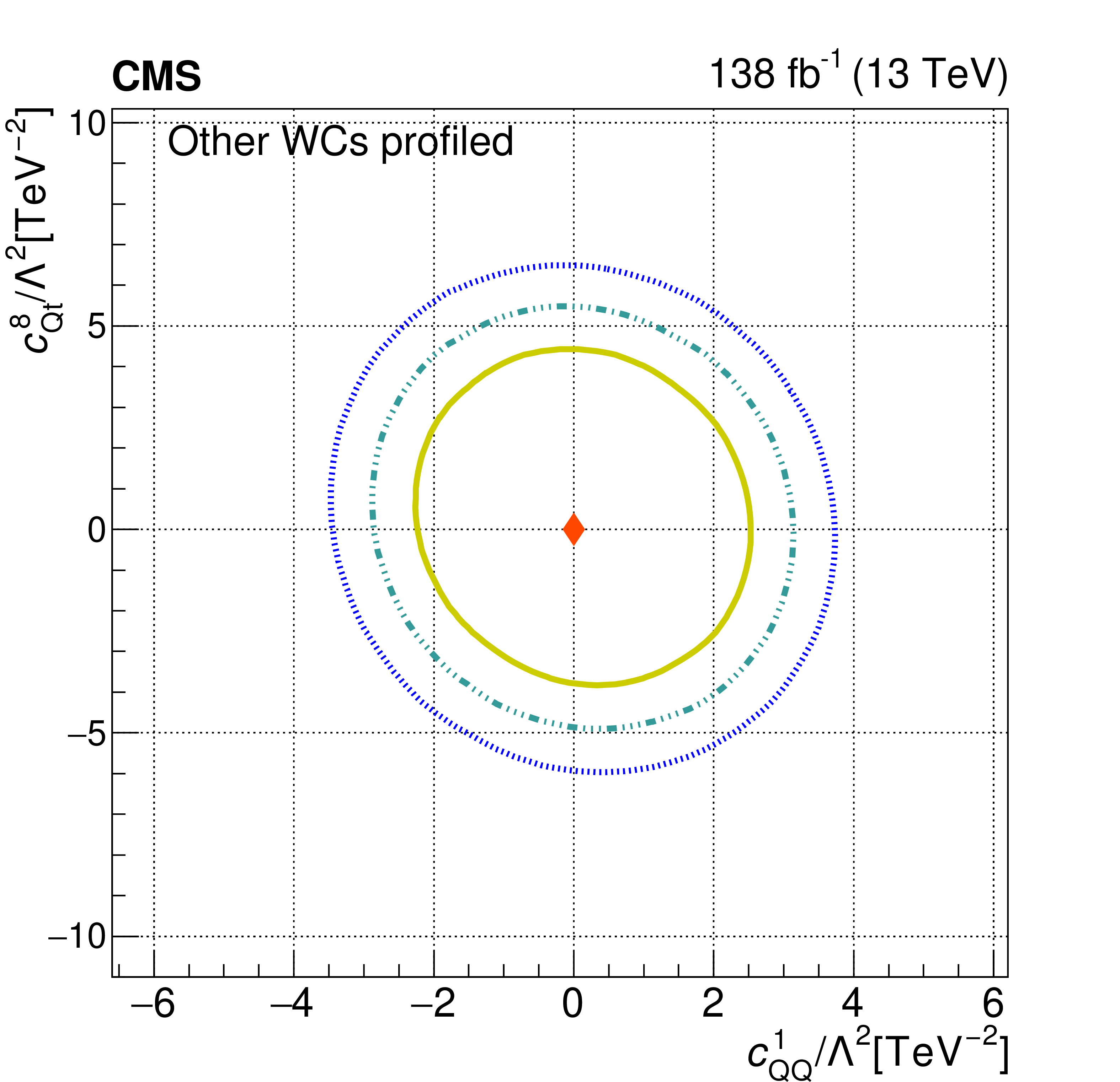
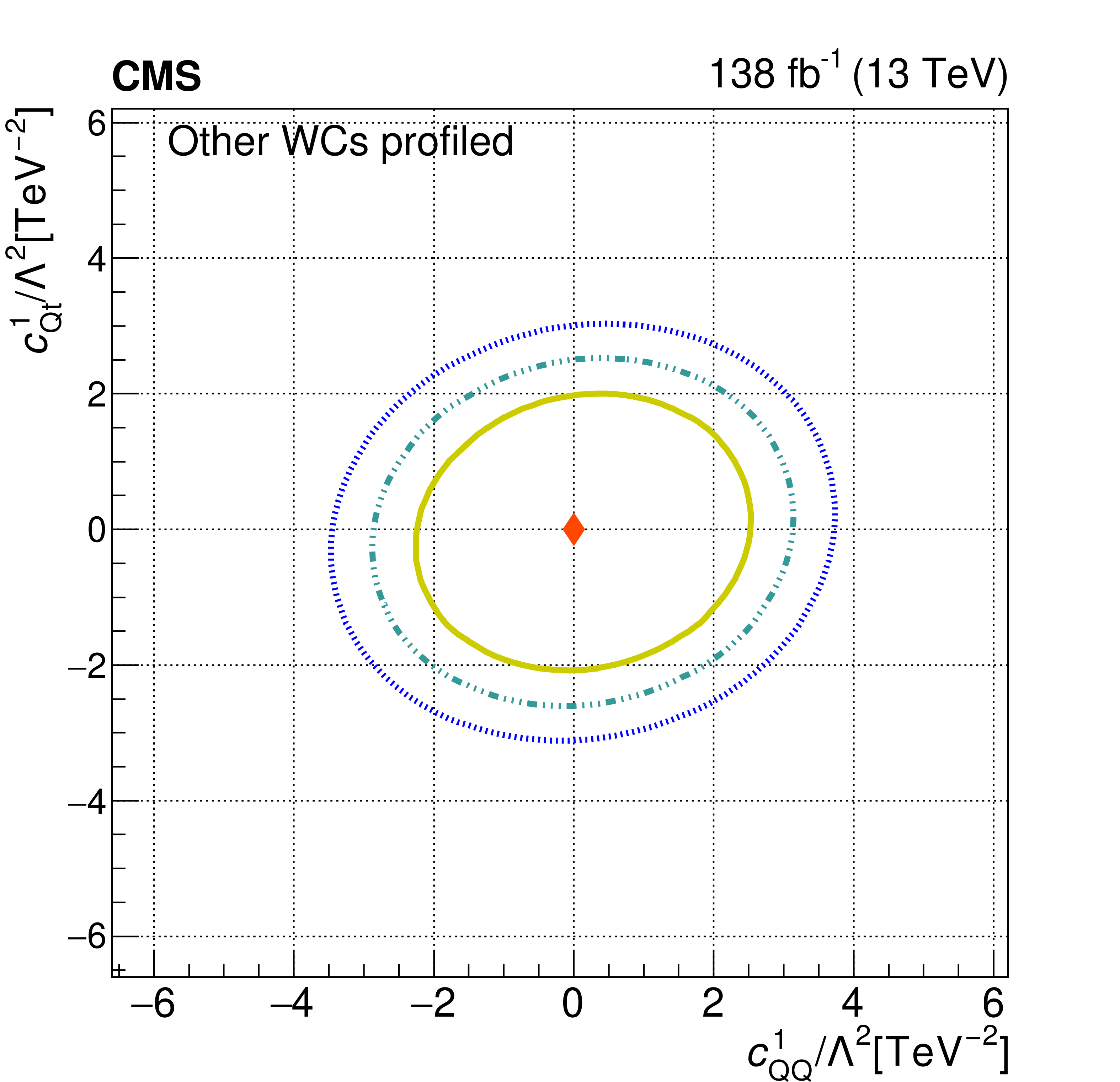
Figure 11:
The observed 68.3, 95.5, and 99.7% confidence level contours of a 2D scan with the other WCs profiled, for $c_{\mathrm{Qt}}^{1}$ and $c_{\mathrm{Qt}}^{8}$ (upper left), for $c_{\mathrm{QQ}}^{8}$ and $c_{\mathrm{Qt}}^{8}$ (upper right), for $c_{\mathrm{Qt}}^{1}$ and $c_{\mathrm{tt}}^{1}$ (lower left), and for $c_{\mathrm{QQ}}^{8}$ and $c_{\mathrm{Qt}}^{1}$ (lower right). Diamond markers show the SM prediction. |

png pdf |
Figure 11-a:
The observed 68.3, 95.5, and 99.7% confidence level contours of a 2D scan with the other WCs profiled, for $c_{\mathrm{Qt}}^{1}$ and $c_{\mathrm{Qt}}^{8}$ (upper left), for $c_{\mathrm{QQ}}^{8}$ and $c_{\mathrm{Qt}}^{8}$ (upper right), for $c_{\mathrm{Qt}}^{1}$ and $c_{\mathrm{tt}}^{1}$ (lower left), and for $c_{\mathrm{QQ}}^{8}$ and $c_{\mathrm{Qt}}^{1}$ (lower right). Diamond markers show the SM prediction. |

png pdf |
Figure 11-b:
The observed 68.3, 95.5, and 99.7% confidence level contours of a 2D scan with the other WCs profiled, for $c_{\mathrm{Qt}}^{1}$ and $c_{\mathrm{Qt}}^{8}$ (upper left), for $c_{\mathrm{QQ}}^{8}$ and $c_{\mathrm{Qt}}^{8}$ (upper right), for $c_{\mathrm{Qt}}^{1}$ and $c_{\mathrm{tt}}^{1}$ (lower left), and for $c_{\mathrm{QQ}}^{8}$ and $c_{\mathrm{Qt}}^{1}$ (lower right). Diamond markers show the SM prediction. |
png pdf |
Figure 11-c:
The observed 68.3, 95.5, and 99.7% confidence level contours of a 2D scan with the other WCs profiled, for $c_{\mathrm{Qt}}^{1}$ and $c_{\mathrm{Qt}}^{8}$ (upper left), for $c_{\mathrm{QQ}}^{8}$ and $c_{\mathrm{Qt}}^{8}$ (upper right), for $c_{\mathrm{Qt}}^{1}$ and $c_{\mathrm{tt}}^{1}$ (lower left), and for $c_{\mathrm{QQ}}^{8}$ and $c_{\mathrm{Qt}}^{1}$ (lower right). Diamond markers show the SM prediction. |

png pdf |
Figure 11-d:
The observed 68.3, 95.5, and 99.7% confidence level contours of a 2D scan with the other WCs profiled, for $c_{\mathrm{Qt}}^{1}$ and $c_{\mathrm{Qt}}^{8}$ (upper left), for $c_{\mathrm{QQ}}^{8}$ and $c_{\mathrm{Qt}}^{8}$ (upper right), for $c_{\mathrm{Qt}}^{1}$ and $c_{\mathrm{tt}}^{1}$ (lower left), and for $c_{\mathrm{QQ}}^{8}$ and $c_{\mathrm{Qt}}^{1}$ (lower right). Diamond markers show the SM prediction. |
png pdf |
Figure 11-e:
The observed 68.3, 95.5, and 99.7% confidence level contours of a 2D scan with the other WCs profiled, for $c_{\mathrm{Qt}}^{1}$ and $c_{\mathrm{Qt}}^{8}$ (upper left), for $c_{\mathrm{QQ}}^{8}$ and $c_{\mathrm{Qt}}^{8}$ (upper right), for $c_{\mathrm{Qt}}^{1}$ and $c_{\mathrm{tt}}^{1}$ (lower left), and for $c_{\mathrm{QQ}}^{8}$ and $c_{\mathrm{Qt}}^{1}$ (lower right). Diamond markers show the SM prediction. |
| Tables | |

png pdf |
Table 1:
List of Wilson coefficients (WCs) included in this analysis, grouped according to the categories of WCs defined in Ref. [22]; the abbreviations for the WCs categories used in this paper are noted parenthetically. The definitions of the WCs and the definitions of the corresponding operators can be found in Table 1 of Ref. [22]. An extra factor of the strong coupling is applied to the $c_{\mathrm{tG}}$ coefficient, as explained in the text. |

png pdf |
Table 2:
Theoretical cross sections at next-to-LO (NLO) used for normalization of simulated signal samples. The items are ordered by cross section. The uncertainties are broken into normalization components due to modeling the parton distribution functions (PDFs) and QCD order. Entries without a value are negligible. |

png pdf |
Table 3:
Object requirements for the 43 event selection categories. Requirements separated by commas indicate a division into subcategories. The kinematical variable that is used in the event category is also listed. Section 5.4 provides further details regarding the kinematical distributions. |

png pdf |
Table 4:
Summary of systematic uncertainties along with the average change in the SM prediction yields |

png pdf |
Table 5:
The 1$ \sigma $ uncertainty intervals extracted from the likelihood fits described in Section 7. The intervals are shown for the case where the other Wilson coefficients (WCs) are profiled, and the case where the other WCs are fixed to their SM values of zero. |

png pdf |
Table 6:
The 2$ \sigma $ uncertainty intervals extracted from the likelihood fits described in Section 7. The intervals are shown for the case where the other Wilson coefficients (WCs) are profiled, and the case where the other WCs are fixed to their SM values of zero. |

png pdf |
Table 7:
Summary of categories that provide leading contributions to the sensitivity for subsets of the Wilson coefficients (WCs). |
| Summary |
| A search for new physics in the production of one or more top quarks with additional leptons, jets, and b jets in the context of effective field theory (EFT) has been performed. Events from proton-proton collisions with a center-of-mass energy of 13 TeV corresponding to an integrated luminosity of 138 fb$ ^{-1} $ are used. EFT effects are incorporated into the event weights of the simulated samples, allowing detector-level predictions that account for correlations and interference effects among EFT operators and between EFT operators and standard model (SM) processes. The Wilson coefficients (WCs) corresponding to 26 EFT operators were simultaneously fit to the data. Confidence intervals were extracted for the WCs either individually or in pairs by scanning the likelihood with the other WCs either profiled or fixed at their SM values of zero. In all cases, the data are found to be consistent with the SM expectations. |
| Additional Figures | |

png pdf |
Additional Figure 1:
The 95% profiled limits for each Wilson coefficient ($ c_i $) interpreted in terms of the energy scale $ \Lambda $ for three different assumptions for the value of the coefficient as indicated in the legend. For limits that are not symmetrical around the SM value of zero, the absolute value of the looser limit is used. The definition of the operator associated with $c_{\mathrm{tG}}$ here includes an explicit factor of the strong coupling constant, which should be accounted for when comparing to results extracted based on other conventions. |

png pdf |
Additional Figure 2:
The 95% profiled limits for each Wilson coefficient ($ c_i $) interpreted in terms of the energy scale $ \Lambda $ for the value of the coefficient set to 1. For limits that are not symmetrical around the SM value of zero, the absolute value of the looser limit is used. The definition of the operator associated with $c_{\mathrm{tG}}$ here includes an explicit factor of the strong coupling constant, which should be accounted for when comparing to results extracted based on other conventions. |

png pdf |
Additional Figure 3:
One-dimensional scan over the $c_{\mathrm{bW}}$ Wilson coefficient (WC). The red points correspond to the case where the other WCs are fixed to their SM values of zero, while the black points correspond to the case where the other WCs are profiled. |

png pdf |
Additional Figure 3-a:
One-dimensional scan over the $c_{\mathrm{bW}}$ Wilson coefficient (WC). The red points correspond to the case where the other WCs are fixed to their SM values of zero, while the black points correspond to the case where the other WCs are profiled. |

png pdf |
Additional Figure 3-b:
One-dimensional scan over the $c_{\mathrm{bW}}$ Wilson coefficient (WC). The red points correspond to the case where the other WCs are fixed to their SM values of zero, while the black points correspond to the case where the other WCs are profiled. |
png pdf |
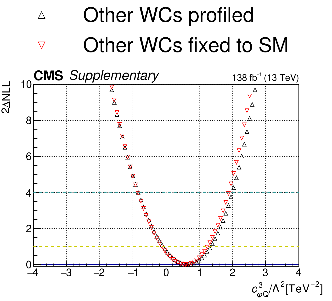
Additional Figure 4:
One-dimensional scan over the $c_{\mathrm{\varphi Q}}^{3}$ Wilson coefficient (WC). The red points correspond to the case where the other WCs are fixed to their SM values of zero, while the black points correspond to the case where the other WCs are profiled. |

png pdf |
Additional Figure 4-a:
One-dimensional scan over the $c_{\mathrm{\varphi Q}}^{3}$ Wilson coefficient (WC). The red points correspond to the case where the other WCs are fixed to their SM values of zero, while the black points correspond to the case where the other WCs are profiled. |

png pdf |
Additional Figure 4-b:
One-dimensional scan over the $c_{\mathrm{\varphi Q}}^{3}$ Wilson coefficient (WC). The red points correspond to the case where the other WCs are fixed to their SM values of zero, while the black points correspond to the case where the other WCs are profiled. |

png pdf |
Additional Figure 5:
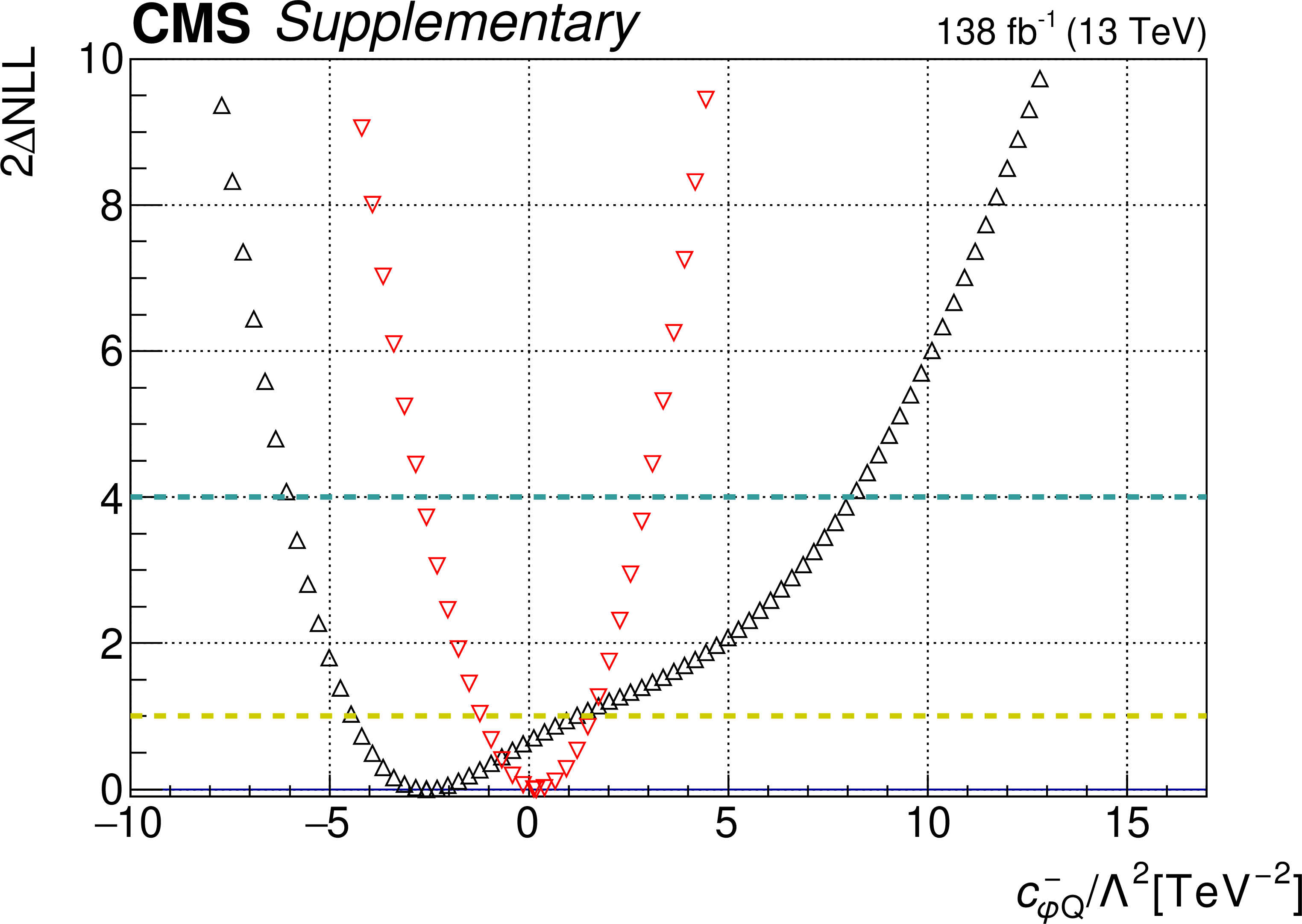
One-dimensional scan over the $c_{\mathrm{\varphi Q}}^{-}$ Wilson coefficient (WC). The red points correspond to the case where the other WCs are fixed to their SM values of zero, while the black points correspond to the case where the other WCs are profiled. |

png pdf |
Additional Figure 5-a:
One-dimensional scan over the $c_{\mathrm{\varphi Q}}^{-}$ Wilson coefficient (WC). The red points correspond to the case where the other WCs are fixed to their SM values of zero, while the black points correspond to the case where the other WCs are profiled. |
png pdf |
Additional Figure 5-b:
One-dimensional scan over the $c_{\mathrm{\varphi Q}}^{-}$ Wilson coefficient (WC). The red points correspond to the case where the other WCs are fixed to their SM values of zero, while the black points correspond to the case where the other WCs are profiled. |

png pdf |
Additional Figure 6:
One-dimensional scan over the $c_{\mathrm{\varphi t}}$ Wilson coefficient (WC). The red points correspond to the case where the other WCs are fixed to their SM values of zero, while the black points correspond to the case where the other WCs are profiled. |

png pdf |
Additional Figure 6-a:
One-dimensional scan over the $c_{\mathrm{\varphi t}}$ Wilson coefficient (WC). The red points correspond to the case where the other WCs are fixed to their SM values of zero, while the black points correspond to the case where the other WCs are profiled. |

png pdf |
Additional Figure 6-b:
One-dimensional scan over the $c_{\mathrm{\varphi t}}$ Wilson coefficient (WC). The red points correspond to the case where the other WCs are fixed to their SM values of zero, while the black points correspond to the case where the other WCs are profiled. |

png pdf |
Additional Figure 7:
One-dimensional scan over the $c_{\mathrm{\varphi tb}}$ Wilson coefficient (WC). The red points correspond to the case where the other WCs are fixed to their SM values of zero, while the black points correspond to the case where the other WCs are profiled. |

png pdf |
Additional Figure 7-a:
One-dimensional scan over the $c_{\mathrm{\varphi tb}}$ Wilson coefficient (WC). The red points correspond to the case where the other WCs are fixed to their SM values of zero, while the black points correspond to the case where the other WCs are profiled. |

png pdf |
Additional Figure 7-b:
One-dimensional scan over the $c_{\mathrm{\varphi tb}}$ Wilson coefficient (WC). The red points correspond to the case where the other WCs are fixed to their SM values of zero, while the black points correspond to the case where the other WCs are profiled. |
png pdf |
Additional Figure 8:
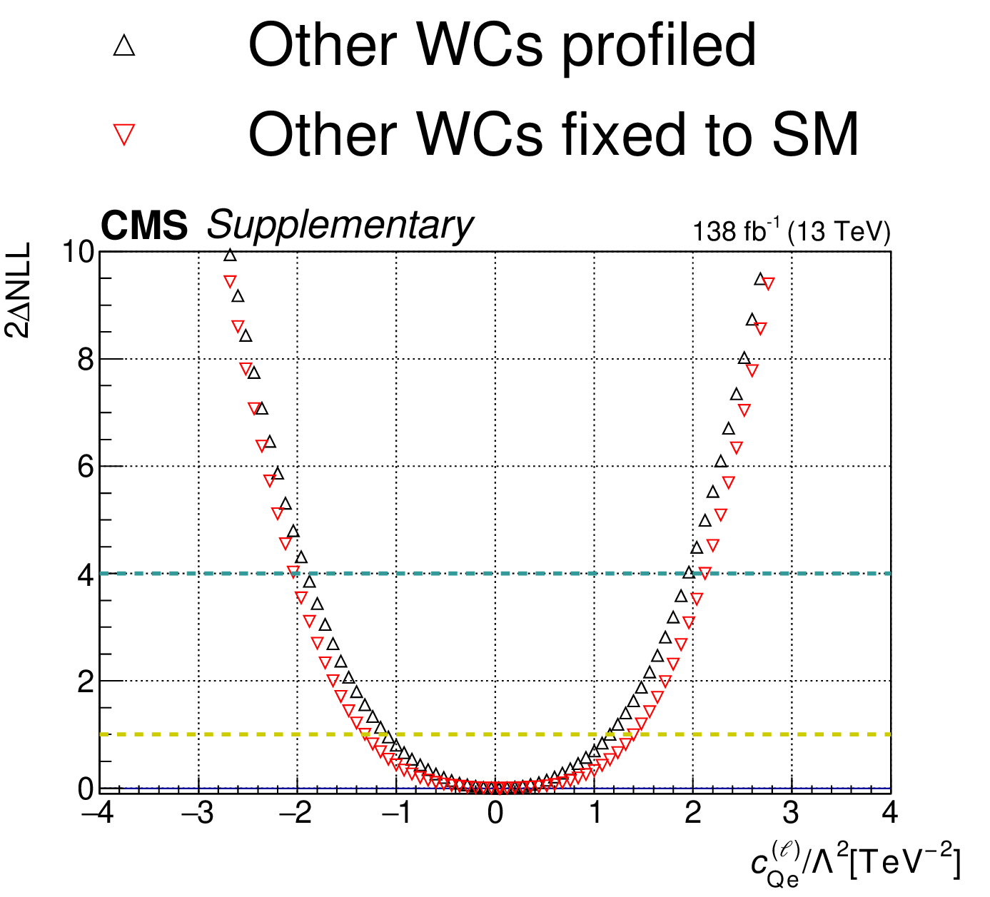
One-dimensional scan over the $c_{\mathrm{qe}}^{(\ell)}$ Wilson coefficient (WC). The red points correspond to the case where the other WCs are fixed to their SM values of zero, while the black points correspond to the case where the other WCs are profiled. |

png pdf |
Additional Figure 8-a:
One-dimensional scan over the $c_{\mathrm{qe}}^{(\ell)}$ Wilson coefficient (WC). The red points correspond to the case where the other WCs are fixed to their SM values of zero, while the black points correspond to the case where the other WCs are profiled. |

png pdf |
Additional Figure 8-b:
One-dimensional scan over the $c_{\mathrm{qe}}^{(\ell)}$ Wilson coefficient (WC). The red points correspond to the case where the other WCs are fixed to their SM values of zero, while the black points correspond to the case where the other WCs are profiled. |

png pdf |
Additional Figure 9:
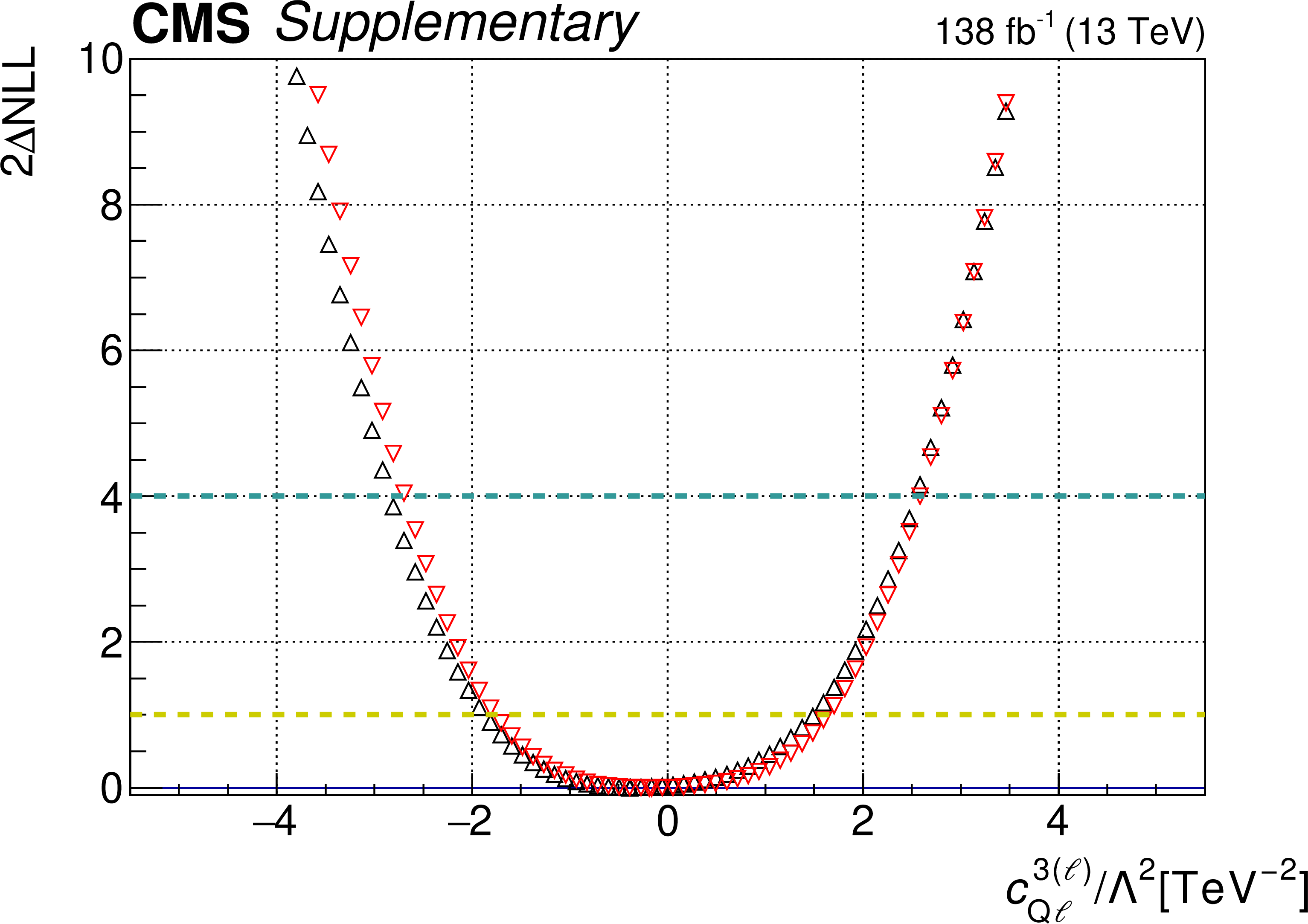
One-dimensional scan over the $c_{\mathrm{Q\ell}}^{3(\ell)}$Wilson coefficient (WC). The red points correspond to the case where the other WCs are fixed to their SM values of zero, while the black points correspond to the case where the other WCs are profiled. |
png pdf |
Additional Figure 9-a:
One-dimensional scan over the $c_{\mathrm{Q\ell}}^{3(\ell)}$Wilson coefficient (WC). The red points correspond to the case where the other WCs are fixed to their SM values of zero, while the black points correspond to the case where the other WCs are profiled. |
png pdf |
Additional Figure 9-b:
One-dimensional scan over the $c_{\mathrm{Q\ell}}^{3(\ell)}$Wilson coefficient (WC). The red points correspond to the case where the other WCs are fixed to their SM values of zero, while the black points correspond to the case where the other WCs are profiled. |

png pdf |
Additional Figure 10:
One-dimensional scan over the $c_{\mathrm{Q\ell}}^{-(\ell)}$ Wilson coefficient (WC). The red points correspond to the case where the other WCs are fixed to their SM values of zero, while the black points correspond to the case where the other WCs are profiled. |

png pdf |
Additional Figure 10-a:
One-dimensional scan over the $c_{\mathrm{Q\ell}}^{-(\ell)}$ Wilson coefficient (WC). The red points correspond to the case where the other WCs are fixed to their SM values of zero, while the black points correspond to the case where the other WCs are profiled. |

png pdf |
Additional Figure 10-b:
One-dimensional scan over the $c_{\mathrm{Q\ell}}^{-(\ell)}$ Wilson coefficient (WC). The red points correspond to the case where the other WCs are fixed to their SM values of zero, while the black points correspond to the case where the other WCs are profiled. |

png pdf |
Additional Figure 11:
One-dimensional scan over the $c_{\mathrm{Qq}}^{11}$ Wilson coefficient (WC). The red points correspond to the case where the other WCs are fixed to their SM values of zero, while the black points correspond to the case where the other WCs are profiled. |

png pdf |
Additional Figure 11-a:
One-dimensional scan over the $c_{\mathrm{Qq}}^{11}$ Wilson coefficient (WC). The red points correspond to the case where the other WCs are fixed to their SM values of zero, while the black points correspond to the case where the other WCs are profiled. |

png pdf |
Additional Figure 11-b:
One-dimensional scan over the $c_{\mathrm{Qq}}^{11}$ Wilson coefficient (WC). The red points correspond to the case where the other WCs are fixed to their SM values of zero, while the black points correspond to the case where the other WCs are profiled. |

png pdf |
Additional Figure 12:
One-dimensional scan over the $c_{\mathrm{QQ}}^{8}$ Wilson coefficient (WC). The red points correspond to the case where the other WCs are fixed to their SM values of zero, while the black points correspond to the case where the other WCs are profiled. |

png pdf |
Additional Figure 12-a:
One-dimensional scan over the $c_{\mathrm{QQ}}^{8}$ Wilson coefficient (WC). The red points correspond to the case where the other WCs are fixed to their SM values of zero, while the black points correspond to the case where the other WCs are profiled. |

png pdf |
Additional Figure 12-b:
One-dimensional scan over the $c_{\mathrm{QQ}}^{8}$ Wilson coefficient (WC). The red points correspond to the case where the other WCs are fixed to their SM values of zero, while the black points correspond to the case where the other WCs are profiled. |

png pdf |
Additional Figure 13:
One-dimensional scan over the $c_{\mathrm{Qq}}^{31}$ Wilson coefficient (WC). The red points correspond to the case where the other WCs are fixed to their SM values of zero, while the black points correspond to the case where the other WCs are profiled. |

png pdf |
Additional Figure 13-a:
One-dimensional scan over the $c_{\mathrm{Qq}}^{31}$ Wilson coefficient (WC). The red points correspond to the case where the other WCs are fixed to their SM values of zero, while the black points correspond to the case where the other WCs are profiled. |

png pdf |
Additional Figure 13-b:
One-dimensional scan over the $c_{\mathrm{Qq}}^{31}$ Wilson coefficient (WC). The red points correspond to the case where the other WCs are fixed to their SM values of zero, while the black points correspond to the case where the other WCs are profiled. |

png pdf |
Additional Figure 14:
One-dimensional scan over the $c_{\mathrm{Qq}}^{18}$ Wilson coefficient (WC). The red points correspond to the case where the other WCs are fixed to their SM values of zero, while the black points correspond to the case where the other WCs are profiled. |

png pdf |
Additional Figure 14-a:
One-dimensional scan over the $c_{\mathrm{Qq}}^{18}$ Wilson coefficient (WC). The red points correspond to the case where the other WCs are fixed to their SM values of zero, while the black points correspond to the case where the other WCs are profiled. |

png pdf |
Additional Figure 14-b:
One-dimensional scan over the $c_{\mathrm{Qq}}^{18}$ Wilson coefficient (WC). The red points correspond to the case where the other WCs are fixed to their SM values of zero, while the black points correspond to the case where the other WCs are profiled. |

png pdf |
Additional Figure 15:
One-dimensional scan over the $c_{\mathrm{Qq}}^{38}$ Wilson coefficient (WC). The red points correspond to the case where the other WCs are fixed to their SM values of zero, while the black points correspond to the case where the other WCs are profiled. |

png pdf |
Additional Figure 15-a:
One-dimensional scan over the $c_{\mathrm{Qq}}^{38}$ Wilson coefficient (WC). The red points correspond to the case where the other WCs are fixed to their SM values of zero, while the black points correspond to the case where the other WCs are profiled. |

png pdf |
Additional Figure 15-b:
One-dimensional scan over the $c_{\mathrm{Qq}}^{38}$ Wilson coefficient (WC). The red points correspond to the case where the other WCs are fixed to their SM values of zero, while the black points correspond to the case where the other WCs are profiled. |
png pdf |
Additional Figure 16:
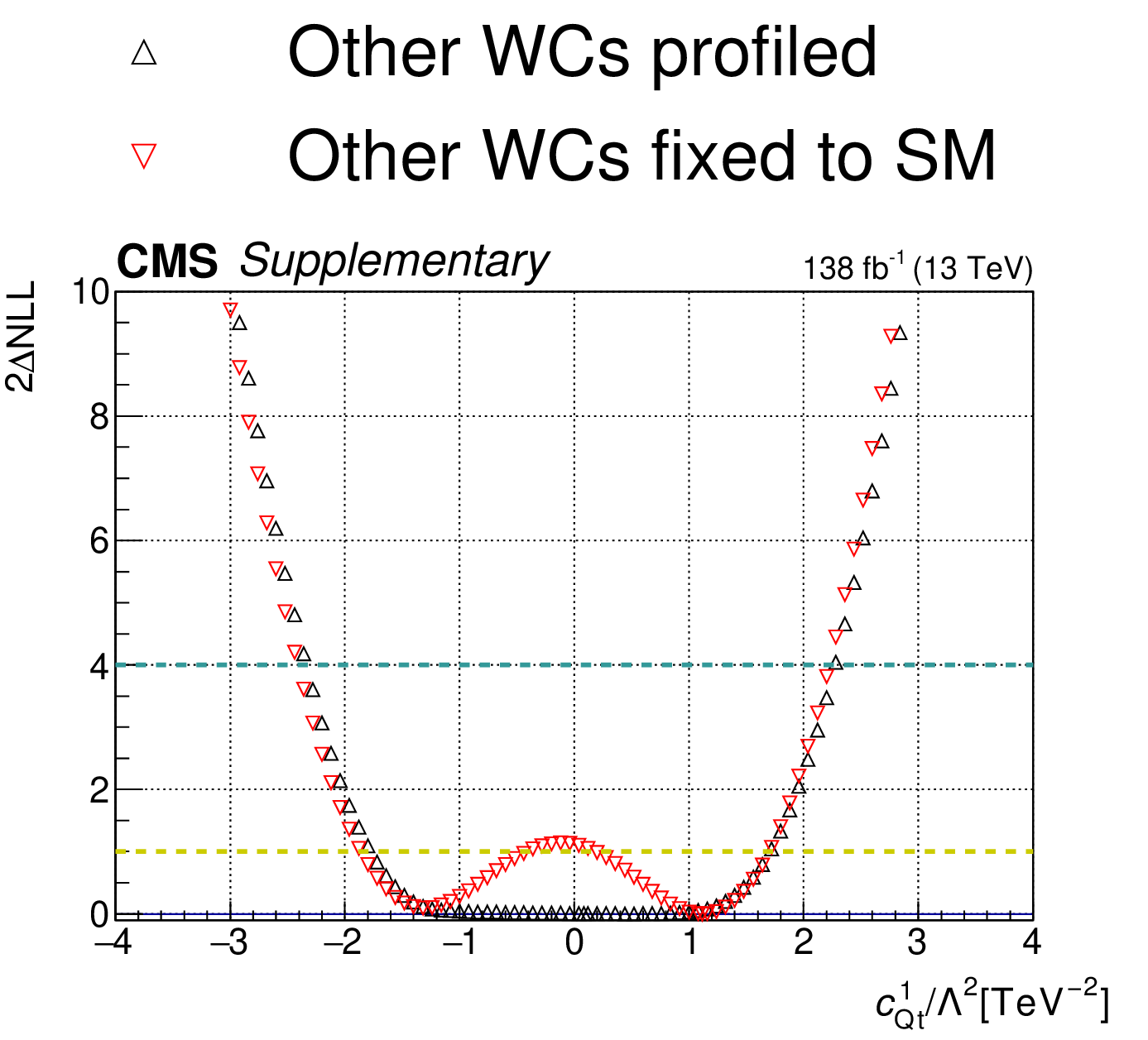
One-dimensional scan over the $c_{\mathrm{Qt}}^{1}$ Wilson coefficient (WC). The red points correspond to the case where the other WCs are fixed to their SM values of zero, while the black points correspond to the case where the other WCs are profiled. |

png pdf |
Additional Figure 16-a:
One-dimensional scan over the $c_{\mathrm{Qt}}^{1}$ Wilson coefficient (WC). The red points correspond to the case where the other WCs are fixed to their SM values of zero, while the black points correspond to the case where the other WCs are profiled. |

png pdf |
Additional Figure 16-b:
One-dimensional scan over the $c_{\mathrm{Qt}}^{1}$ Wilson coefficient (WC). The red points correspond to the case where the other WCs are fixed to their SM values of zero, while the black points correspond to the case where the other WCs are profiled. |
png pdf |
Additional Figure 17:
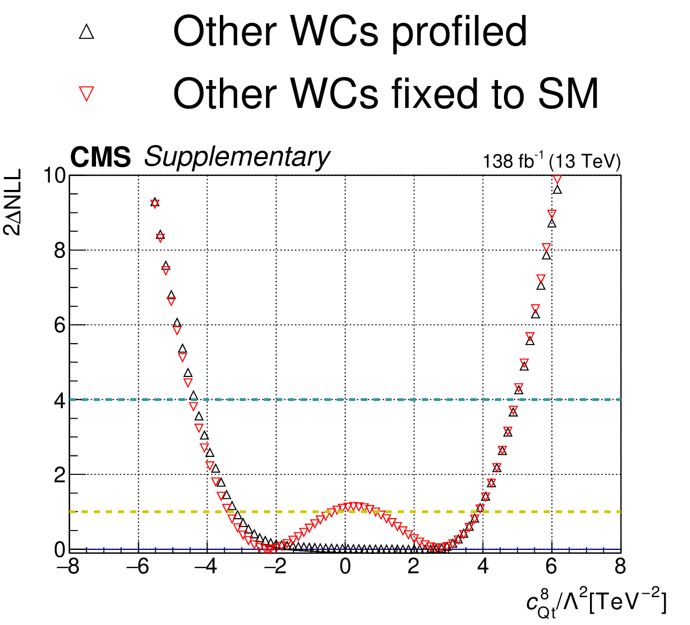
One-dimensional scan over the $c_{\mathrm{Qt}}^{8}$ Wilson coefficient (WC). The red points correspond to the case where the other WCs are fixed to their SM values of zero, while the black points correspond to the case where the other WCs are profiled. |

png pdf |
Additional Figure 17-a:
One-dimensional scan over the $c_{\mathrm{Qt}}^{8}$ Wilson coefficient (WC). The red points correspond to the case where the other WCs are fixed to their SM values of zero, while the black points correspond to the case where the other WCs are profiled. |

png pdf |
Additional Figure 17-b:
One-dimensional scan over the $c_{\mathrm{Qt}}^{8}$ Wilson coefficient (WC). The red points correspond to the case where the other WCs are fixed to their SM values of zero, while the black points correspond to the case where the other WCs are profiled. |

png pdf |
Additional Figure 18:
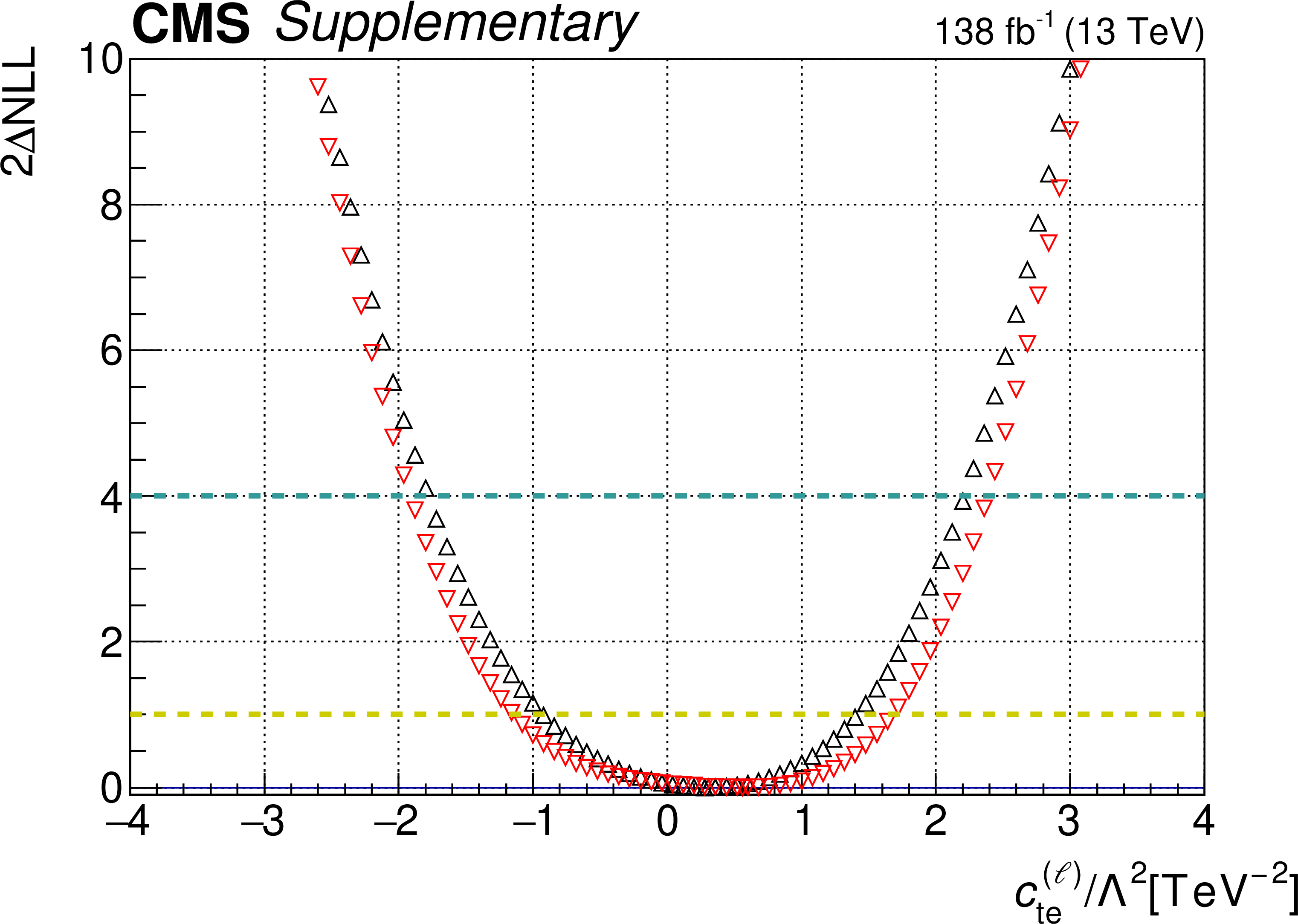
One-dimensional scan over the $c_{\mathrm{te}}^{(\ell)}$ Wilson coefficient (WC). The red points correspond to the case where the other WCs are fixed to their SM values of zero, while the black points correspond to the case where the other WCs are profiled. |

png pdf |
Additional Figure 18-a:
One-dimensional scan over the $c_{\mathrm{te}}^{(\ell)}$ Wilson coefficient (WC). The red points correspond to the case where the other WCs are fixed to their SM values of zero, while the black points correspond to the case where the other WCs are profiled. |
png pdf |
Additional Figure 18-b:
One-dimensional scan over the $c_{\mathrm{te}}^{(\ell)}$ Wilson coefficient (WC). The red points correspond to the case where the other WCs are fixed to their SM values of zero, while the black points correspond to the case where the other WCs are profiled. |
png pdf |
Additional Figure 19:
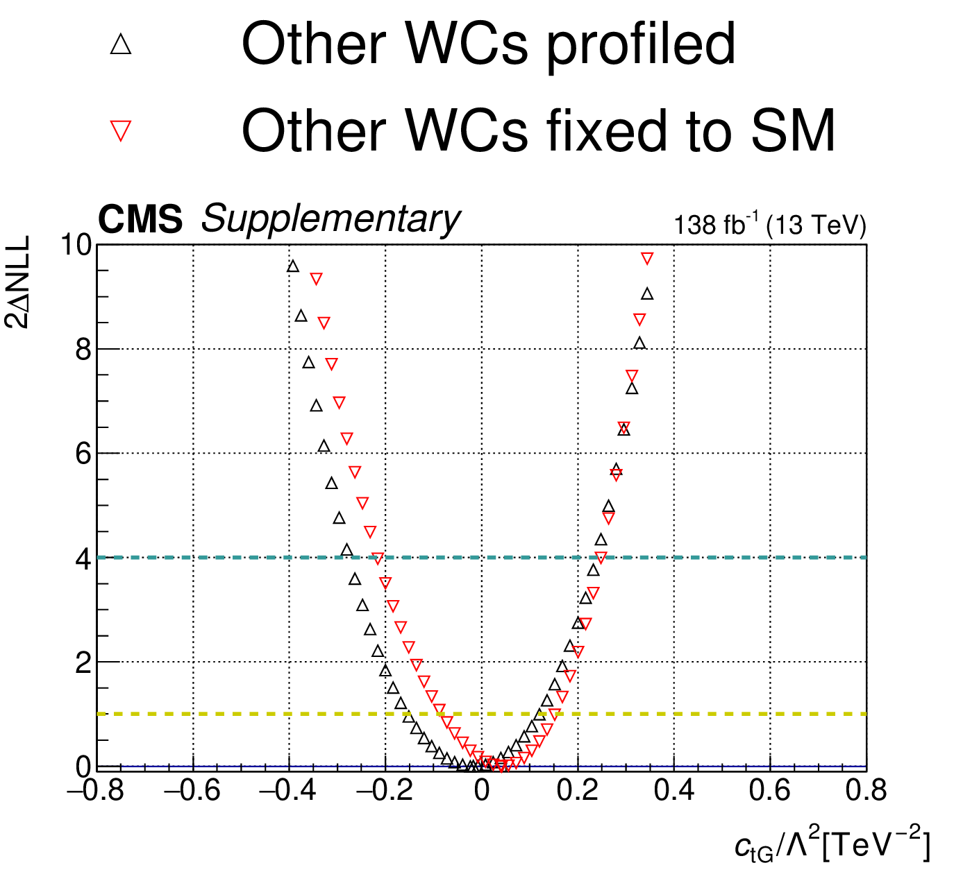
One-dimensional scan over the $c_{\mathrm{tG}}$ Wilson coefficient (WC). The red points correspond to the case where the other WCs are fixed to their SM values of zero, while the black points correspond to the case where the other WCs are profiled. |

png pdf |
Additional Figure 19-a:
One-dimensional scan over the $c_{\mathrm{tG}}$ Wilson coefficient (WC). The red points correspond to the case where the other WCs are fixed to their SM values of zero, while the black points correspond to the case where the other WCs are profiled. |

png pdf |
Additional Figure 19-b:
One-dimensional scan over the $c_{\mathrm{tG}}$ Wilson coefficient (WC). The red points correspond to the case where the other WCs are fixed to their SM values of zero, while the black points correspond to the case where the other WCs are profiled. |

png pdf |
Additional Figure 20:
One-dimensional scan over the $c_{\mathrm{t\ell}}^{(\ell)}$ Wilson coefficient (WC). The red points correspond to the case where the other WCs are fixed to their SM values of zero, while the black points correspond to the case where the other WCs are profiled. |

png pdf |
Additional Figure 20-a:
One-dimensional scan over the $c_{\mathrm{t\ell}}^{(\ell)}$ Wilson coefficient (WC). The red points correspond to the case where the other WCs are fixed to their SM values of zero, while the black points correspond to the case where the other WCs are profiled. |

png pdf |
Additional Figure 20-b:
One-dimensional scan over the $c_{\mathrm{t\ell}}^{(\ell)}$ Wilson coefficient (WC). The red points correspond to the case where the other WCs are fixed to their SM values of zero, while the black points correspond to the case where the other WCs are profiled. |
png pdf |
Additional Figure 21:
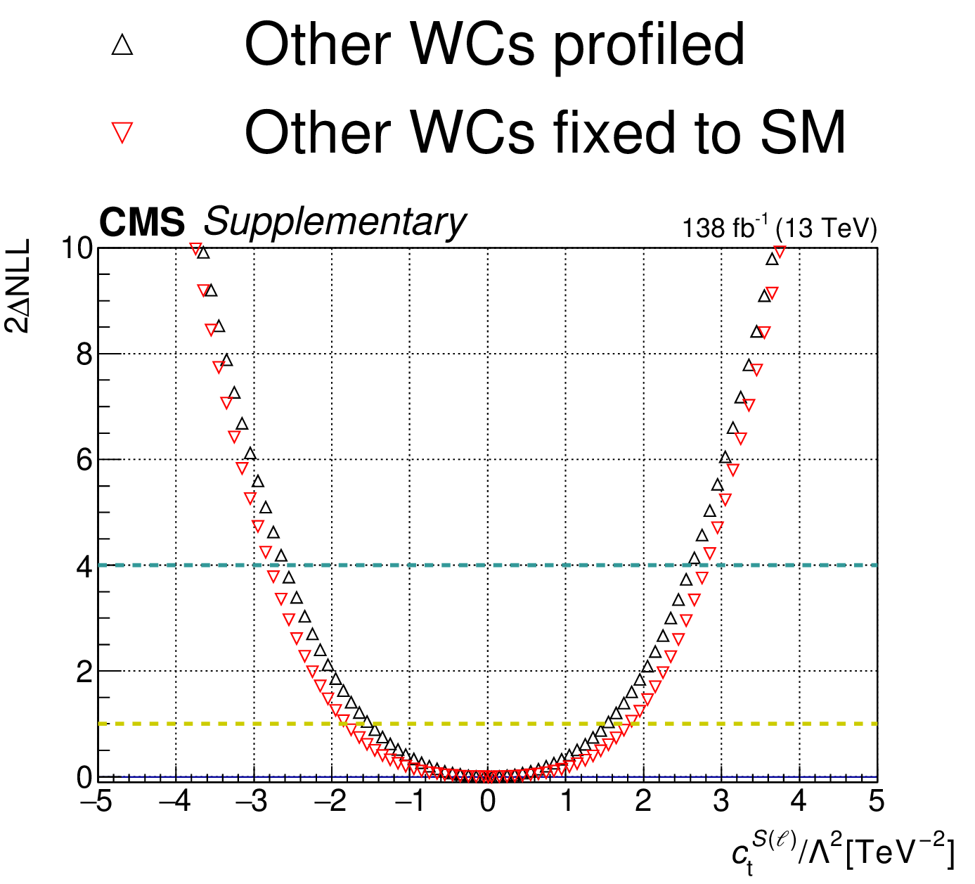
One-dimensional scan over the $c_{\mathrm{t}}^{S(\ell)}$ Wilson coefficient (WC). The red points correspond to the case where the other WCs are fixed to their SM values of zero, while the black points correspond to the case where the other WCs are profiled. |

png pdf |
Additional Figure 21-a:
One-dimensional scan over the $c_{\mathrm{t}}^{S(\ell)}$ Wilson coefficient (WC). The red points correspond to the case where the other WCs are fixed to their SM values of zero, while the black points correspond to the case where the other WCs are profiled. |

png pdf |
Additional Figure 21-b:
One-dimensional scan over the $c_{\mathrm{t}}^{S(\ell)}$ Wilson coefficient (WC). The red points correspond to the case where the other WCs are fixed to their SM values of zero, while the black points correspond to the case where the other WCs are profiled. |
png pdf |
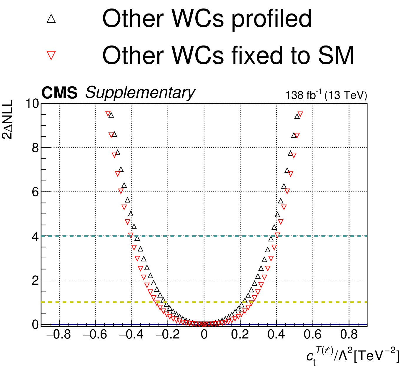
Additional Figure 22:
One-dimensional scan over the $c_{\mathrm{t}}^{T(\ell)}$ Wilson coefficient (WC). The red points correspond to the case where the other WCs are fixed to their SM values of zero, while the black points correspond to the case where the other WCs are profiled. |

png pdf |
Additional Figure 22-a:
One-dimensional scan over the $c_{\mathrm{t}}^{T(\ell)}$ Wilson coefficient (WC). The red points correspond to the case where the other WCs are fixed to their SM values of zero, while the black points correspond to the case where the other WCs are profiled. |

png pdf |
Additional Figure 22-b:
One-dimensional scan over the $c_{\mathrm{t}}^{T(\ell)}$ Wilson coefficient (WC). The red points correspond to the case where the other WCs are fixed to their SM values of zero, while the black points correspond to the case where the other WCs are profiled. |

png pdf |
Additional Figure 23:
One-dimensional scan over the $c_{\mathrm{t\varphi}}$ Wilson coefficient (WC). The red points correspond to the case where the other WCs are fixed to their SM values of zero, while the black points correspond to the case where the other WCs are profiled. |

png pdf |
Additional Figure 23-a:
One-dimensional scan over the $c_{\mathrm{t\varphi}}$ Wilson coefficient (WC). The red points correspond to the case where the other WCs are fixed to their SM values of zero, while the black points correspond to the case where the other WCs are profiled. |

png pdf |
Additional Figure 23-b:
One-dimensional scan over the $c_{\mathrm{t\varphi}}$ Wilson coefficient (WC). The red points correspond to the case where the other WCs are fixed to their SM values of zero, while the black points correspond to the case where the other WCs are profiled. |

png pdf |
Additional Figure 24:
One-dimensional scan over the $c_{\mathrm{tQ}}^{1}$ Wilson coefficient (WC). The red points correspond to the case where the other WCs are fixed to their SM values of zero, while the black points correspond to the case where the other WCs are profiled. |

png pdf |
Additional Figure 24-a:
One-dimensional scan over the $c_{\mathrm{tQ}}^{1}$ Wilson coefficient (WC). The red points correspond to the case where the other WCs are fixed to their SM values of zero, while the black points correspond to the case where the other WCs are profiled. |

png pdf |
Additional Figure 24-b:
One-dimensional scan over the $c_{\mathrm{tQ}}^{1}$ Wilson coefficient (WC). The red points correspond to the case where the other WCs are fixed to their SM values of zero, while the black points correspond to the case where the other WCs are profiled. |

png pdf |
Additional Figure 25:
One-dimensional scan over the $c_{\mathrm{tq}}^{8}$ Wilson coefficient (WC). The red points correspond to the case where the other WCs are fixed to their SM values of zero, while the black points correspond to the case where the other WCs are profiled. |

png pdf |
Additional Figure 25-a:
One-dimensional scan over the $c_{\mathrm{tq}}^{8}$ Wilson coefficient (WC). The red points correspond to the case where the other WCs are fixed to their SM values of zero, while the black points correspond to the case where the other WCs are profiled. |

png pdf |
Additional Figure 25-b:
One-dimensional scan over the $c_{\mathrm{tq}}^{8}$ Wilson coefficient (WC). The red points correspond to the case where the other WCs are fixed to their SM values of zero, while the black points correspond to the case where the other WCs are profiled. |

png pdf |
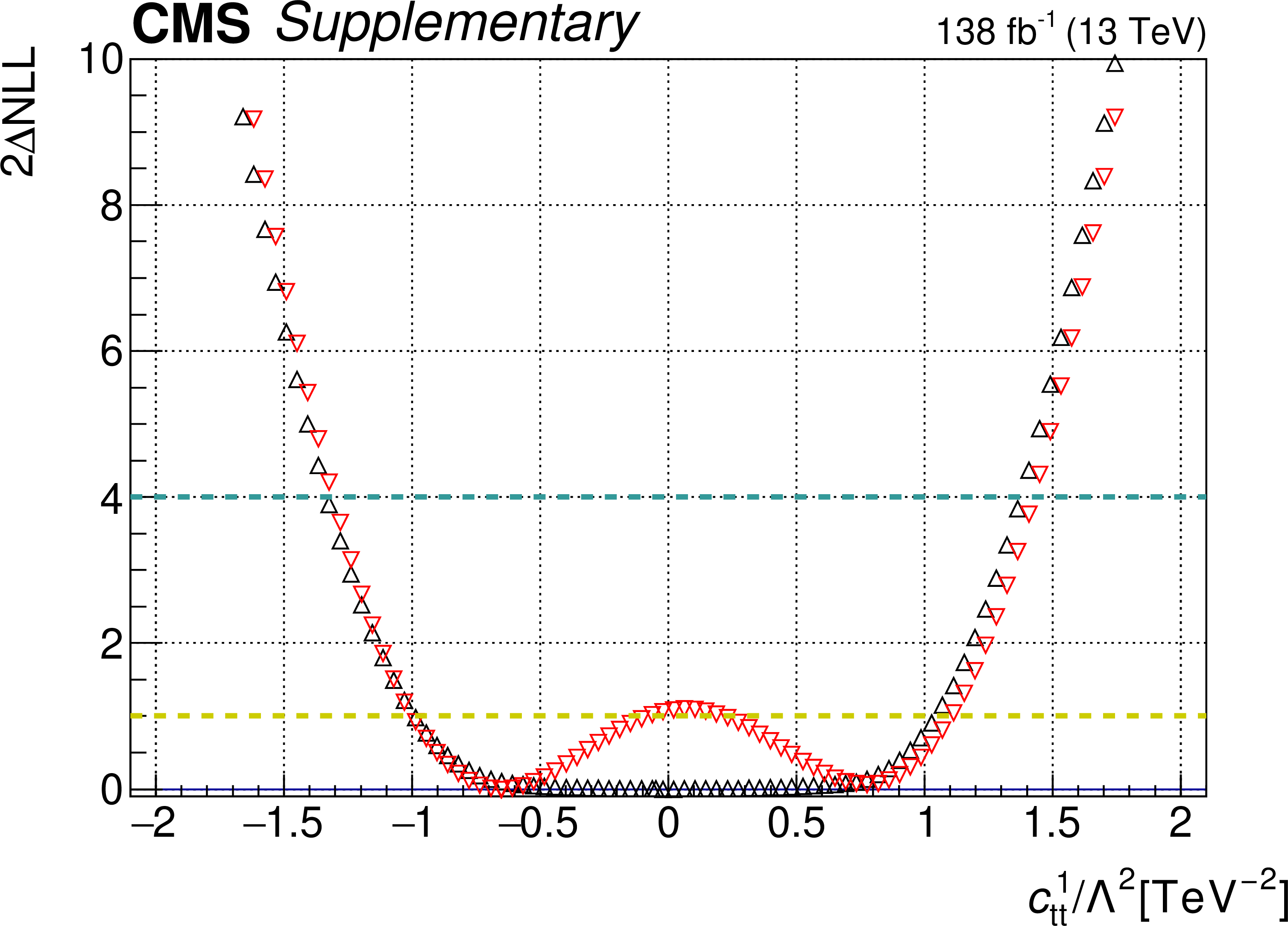
Additional Figure 26:
One-dimensional scan over the $c_{\mathrm{tt}}^{1}$ Wilson coefficient (WC). The red points correspond to the case where the other WCs are fixed to their SM values of zero, while the black points correspond to the case where the other WCs are profiled. |

png pdf |
Additional Figure 26-a:
One-dimensional scan over the $c_{\mathrm{tt}}^{1}$ Wilson coefficient (WC). The red points correspond to the case where the other WCs are fixed to their SM values of zero, while the black points correspond to the case where the other WCs are profiled. |
png pdf |
Additional Figure 26-b:
One-dimensional scan over the $c_{\mathrm{tt}}^{1}$ Wilson coefficient (WC). The red points correspond to the case where the other WCs are fixed to their SM values of zero, while the black points correspond to the case where the other WCs are profiled. |

png pdf |
Additional Figure 27:
One-dimensional scan over the $c_{\mathrm{tW}}$ Wilson coefficient (WC). The red points correspond to the case where the other WCs are fixed to their SM values of zero, while the black points correspond to the case where the other WCs are profiled. |

png pdf |
Additional Figure 27-a:
One-dimensional scan over the $c_{\mathrm{tW}}$ Wilson coefficient (WC). The red points correspond to the case where the other WCs are fixed to their SM values of zero, while the black points correspond to the case where the other WCs are profiled. |

png pdf |
Additional Figure 27-b:
One-dimensional scan over the $c_{\mathrm{tW}}$ Wilson coefficient (WC). The red points correspond to the case where the other WCs are fixed to their SM values of zero, while the black points correspond to the case where the other WCs are profiled. |

png pdf |
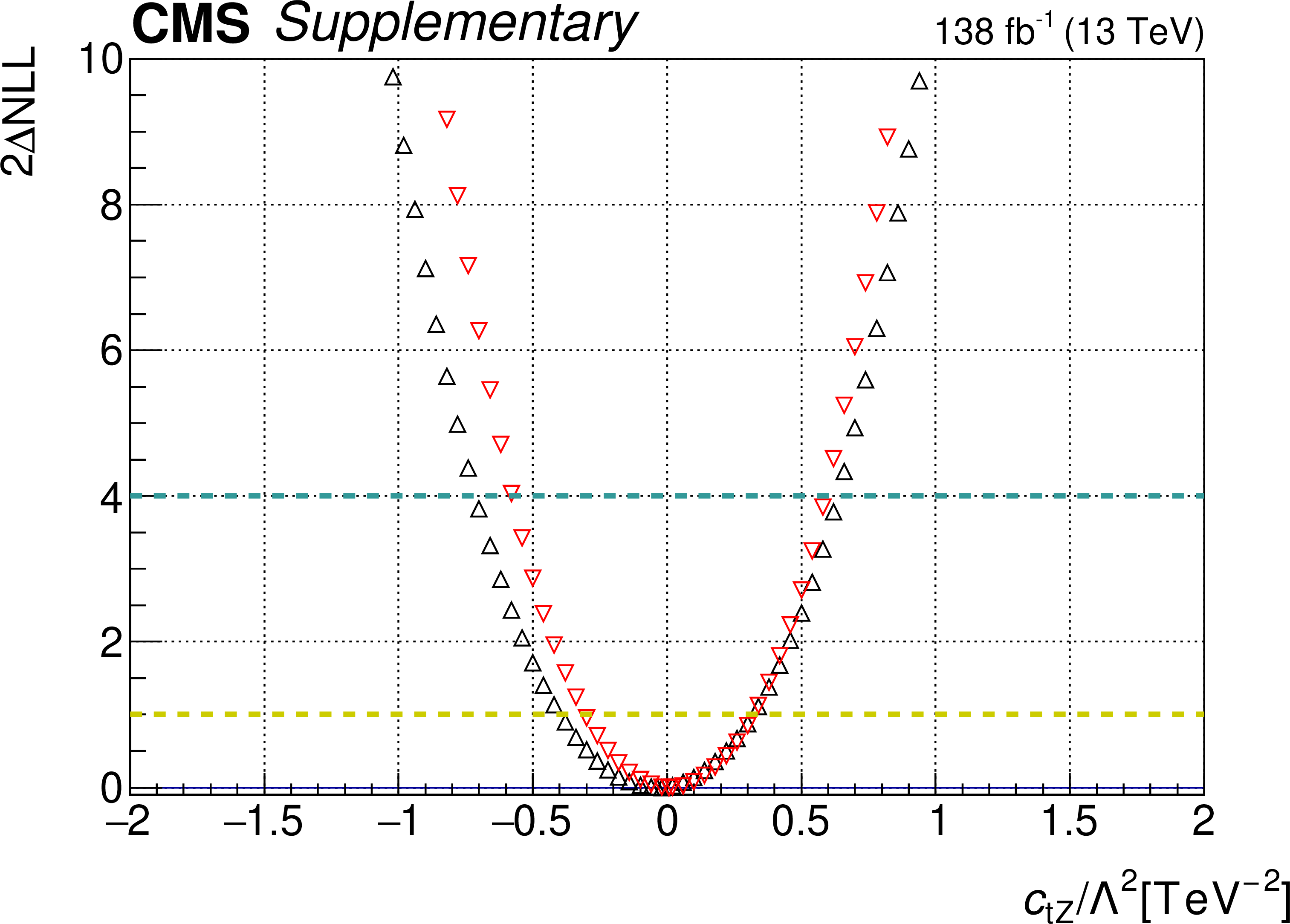
Additional Figure 28:
One-dimensional scan over the $c_{\mathrm{tZ}}$ Wilson coefficient (WC). The red points correspond to the case where the other WCs are fixed to their SM values of zero, while the black points correspond to the case where the other WCs are profiled. |

png pdf |
Additional Figure 28-a:
One-dimensional scan over the $c_{\mathrm{tZ}}$ Wilson coefficient (WC). The red points correspond to the case where the other WCs are fixed to their SM values of zero, while the black points correspond to the case where the other WCs are profiled. |
png pdf |
Additional Figure 28-b:
One-dimensional scan over the $c_{\mathrm{tZ}}$ Wilson coefficient (WC). The red points correspond to the case where the other WCs are fixed to their SM values of zero, while the black points correspond to the case where the other WCs are profiled. |
png pdf |
Additional Figure 29:
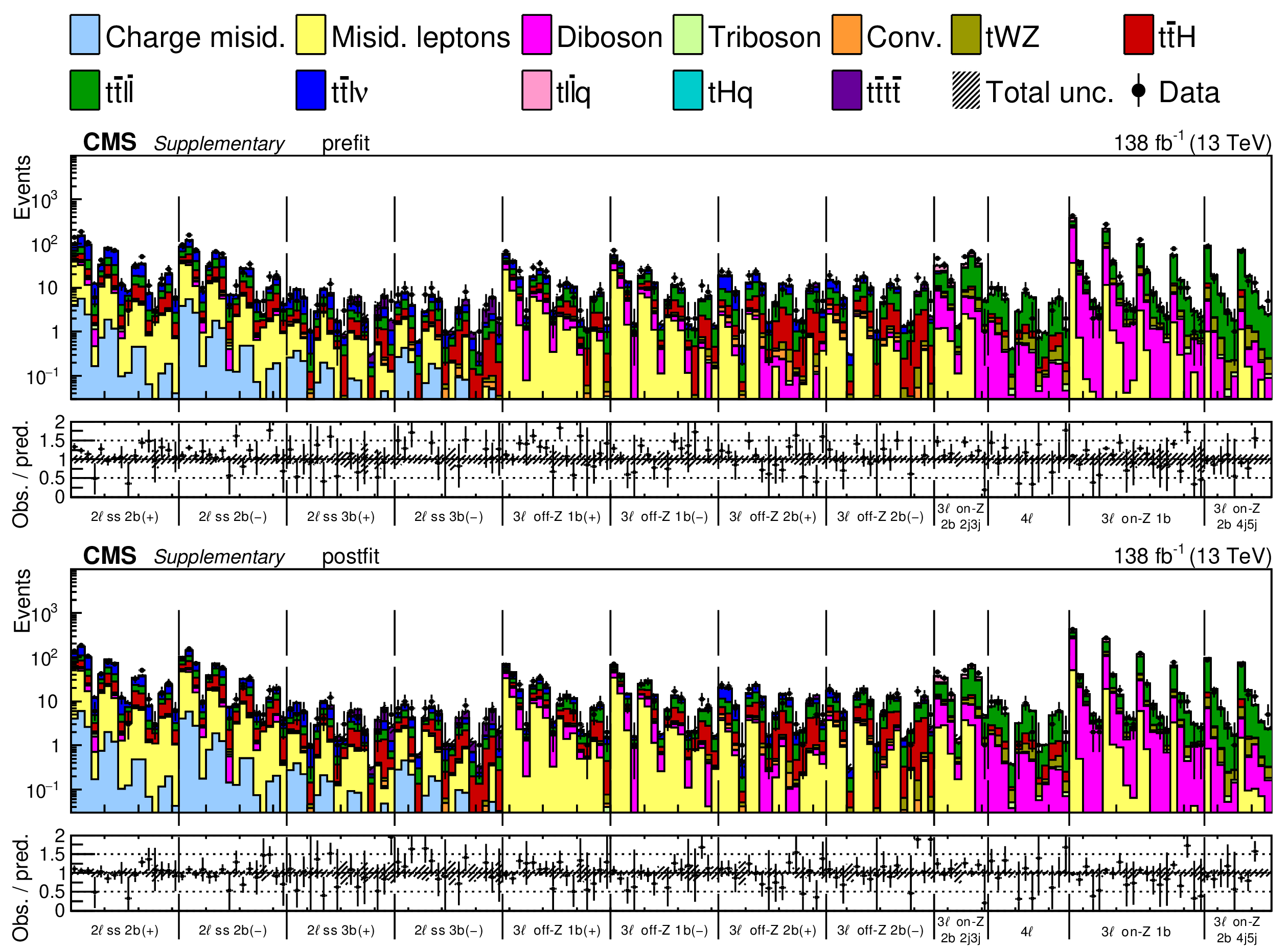
Observed data and expected yields in the prefit (upper) and postfit (lower) scenarios. All kinematic variables are shown. The two categories on the right side of the plot (3$ \ell $ on-Z 1b, and the 4 and 5 jet bins of 3$ \ell $ on-Z 2b) use the $ {p_{\mathrm{T}}}\mathrm{(\mathrm{Z})} $ variable, while all the other categories use $ {p_{\mathrm{T}}}\mathrm{(\ell j )_{\rm max}} $. Each event category (e.g., 2 $ \ell \textrm{ss} $) is subdivided into its jet multiplcity components. For example, the first four subbins of the 2 $ \ell \textrm{ss} $ bin are the $ {p_{\mathrm{T}}}\mathrm{(\ell j )_{\rm max}} $ variable for four jets, the next four subbins are the $ {p_{\mathrm{T}}}\mathrm{(\ell j )_{\rm max}} $ variable for 5 jets, etc. The postfit values are obtained by simultaneously fitting all $ \mathrm{26} $ Wilson coefficient (WCs) and the nuisance parameters (NPs). The process labeled ``Conv." corresponds to the photon conversion background, ``Misid. leptons" corresponds to misidentified leptons, and ``Charge misid." corresponds to leptons with a mismeasured charge. The lower panel contains the ratios of the observed yields over the expected. The error bands are computed by propagating the uncertainties from the WCs and NPs. All yields are plotted on a log scale. |

png pdf |
Additional Figure 29-a:
Observed data and expected yields in the prefit (upper) and postfit (lower) scenarios. All kinematic variables are shown. The two categories on the right side of the plot (3$ \ell $ on-Z 1b, and the 4 and 5 jet bins of 3$ \ell $ on-Z 2b) use the $ {p_{\mathrm{T}}}\mathrm{(\mathrm{Z})} $ variable, while all the other categories use $ {p_{\mathrm{T}}}\mathrm{(\ell j )_{\rm max}} $. Each event category (e.g., 2 $ \ell \textrm{ss} $) is subdivided into its jet multiplcity components. For example, the first four subbins of the 2 $ \ell \textrm{ss} $ bin are the $ {p_{\mathrm{T}}}\mathrm{(\ell j )_{\rm max}} $ variable for four jets, the next four subbins are the $ {p_{\mathrm{T}}}\mathrm{(\ell j )_{\rm max}} $ variable for 5 jets, etc. The postfit values are obtained by simultaneously fitting all $ \mathrm{26} $ Wilson coefficient (WCs) and the nuisance parameters (NPs). The process labeled ``Conv." corresponds to the photon conversion background, ``Misid. leptons" corresponds to misidentified leptons, and ``Charge misid." corresponds to leptons with a mismeasured charge. The lower panel contains the ratios of the observed yields over the expected. The error bands are computed by propagating the uncertainties from the WCs and NPs. All yields are plotted on a log scale. |

png pdf |
Additional Figure 29-b:
Observed data and expected yields in the prefit (upper) and postfit (lower) scenarios. All kinematic variables are shown. The two categories on the right side of the plot (3$ \ell $ on-Z 1b, and the 4 and 5 jet bins of 3$ \ell $ on-Z 2b) use the $ {p_{\mathrm{T}}}\mathrm{(\mathrm{Z})} $ variable, while all the other categories use $ {p_{\mathrm{T}}}\mathrm{(\ell j )_{\rm max}} $. Each event category (e.g., 2 $ \ell \textrm{ss} $) is subdivided into its jet multiplcity components. For example, the first four subbins of the 2 $ \ell \textrm{ss} $ bin are the $ {p_{\mathrm{T}}}\mathrm{(\ell j )_{\rm max}} $ variable for four jets, the next four subbins are the $ {p_{\mathrm{T}}}\mathrm{(\ell j )_{\rm max}} $ variable for 5 jets, etc. The postfit values are obtained by simultaneously fitting all $ \mathrm{26} $ Wilson coefficient (WCs) and the nuisance parameters (NPs). The process labeled ``Conv." corresponds to the photon conversion background, ``Misid. leptons" corresponds to misidentified leptons, and ``Charge misid." corresponds to leptons with a mismeasured charge. The lower panel contains the ratios of the observed yields over the expected. The error bands are computed by propagating the uncertainties from the WCs and NPs. All yields are plotted on a log scale. |

png pdf |
Additional Figure 29-c:
Observed data and expected yields in the prefit (upper) and postfit (lower) scenarios. All kinematic variables are shown. The two categories on the right side of the plot (3$ \ell $ on-Z 1b, and the 4 and 5 jet bins of 3$ \ell $ on-Z 2b) use the $ {p_{\mathrm{T}}}\mathrm{(\mathrm{Z})} $ variable, while all the other categories use $ {p_{\mathrm{T}}}\mathrm{(\ell j )_{\rm max}} $. Each event category (e.g., 2 $ \ell \textrm{ss} $) is subdivided into its jet multiplcity components. For example, the first four subbins of the 2 $ \ell \textrm{ss} $ bin are the $ {p_{\mathrm{T}}}\mathrm{(\ell j )_{\rm max}} $ variable for four jets, the next four subbins are the $ {p_{\mathrm{T}}}\mathrm{(\ell j )_{\rm max}} $ variable for 5 jets, etc. The postfit values are obtained by simultaneously fitting all $ \mathrm{26} $ Wilson coefficient (WCs) and the nuisance parameters (NPs). The process labeled ``Conv." corresponds to the photon conversion background, ``Misid. leptons" corresponds to misidentified leptons, and ``Charge misid." corresponds to leptons with a mismeasured charge. The lower panel contains the ratios of the observed yields over the expected. The error bands are computed by propagating the uncertainties from the WCs and NPs. All yields are plotted on a log scale. |

png pdf |
Additional Figure 30:
The top row shows the prefit (left) and postfit (right) yields of the channel 2$ \ell\text{ss 2b} \, (+) $. The bottom row shows the prefit (left) and postfit (right) yields of the channel 2$ \ell\text{ss 2b} \, (-) $. Multiple sets of prefit and postfit plots with the alternative kinematic distribution, including this set of $ H_{\mathrm{T}} $ plots, are used to check the effectiveness of the fit. The jet subcategories are arranged from low jet multiplicity to high jet multiplicity from left to right for each individual plot. For example, in the 2$ \ell\text{ss 2b} \, (+) $ plot, the first seven bins are the $ H_{\mathrm{T}} $ variable for 2$ \ell\text{ss 2b} \, (+) \: \mathrm{4j} $, the next seven bins are for 2$ \ell\text{ss 2b} \, (+) \: \mathrm{5j} $, etc. The process labeled ``Conv." corresponds to the photon conversion background, ``Misid. leptons" corresponds to misidentified leptons, and ``Charge misid." corresponds to leptons with a mismeasured charge. The lower panel contains the ratios of the observed yields over the expected. The error bands correspond to nuisance parameter and Wilson coefficient uncertainties added in quadrature. |

png pdf |
Additional Figure 30-a:
The top row shows the prefit (left) and postfit (right) yields of the channel 2$ \ell\text{ss 2b} \, (+) $. The bottom row shows the prefit (left) and postfit (right) yields of the channel 2$ \ell\text{ss 2b} \, (-) $. Multiple sets of prefit and postfit plots with the alternative kinematic distribution, including this set of $ H_{\mathrm{T}} $ plots, are used to check the effectiveness of the fit. The jet subcategories are arranged from low jet multiplicity to high jet multiplicity from left to right for each individual plot. For example, in the 2$ \ell\text{ss 2b} \, (+) $ plot, the first seven bins are the $ H_{\mathrm{T}} $ variable for 2$ \ell\text{ss 2b} \, (+) \: \mathrm{4j} $, the next seven bins are for 2$ \ell\text{ss 2b} \, (+) \: \mathrm{5j} $, etc. The process labeled ``Conv." corresponds to the photon conversion background, ``Misid. leptons" corresponds to misidentified leptons, and ``Charge misid." corresponds to leptons with a mismeasured charge. The lower panel contains the ratios of the observed yields over the expected. The error bands correspond to nuisance parameter and Wilson coefficient uncertainties added in quadrature. |

png pdf |
Additional Figure 30-b:
The top row shows the prefit (left) and postfit (right) yields of the channel 2$ \ell\text{ss 2b} \, (+) $. The bottom row shows the prefit (left) and postfit (right) yields of the channel 2$ \ell\text{ss 2b} \, (-) $. Multiple sets of prefit and postfit plots with the alternative kinematic distribution, including this set of $ H_{\mathrm{T}} $ plots, are used to check the effectiveness of the fit. The jet subcategories are arranged from low jet multiplicity to high jet multiplicity from left to right for each individual plot. For example, in the 2$ \ell\text{ss 2b} \, (+) $ plot, the first seven bins are the $ H_{\mathrm{T}} $ variable for 2$ \ell\text{ss 2b} \, (+) \: \mathrm{4j} $, the next seven bins are for 2$ \ell\text{ss 2b} \, (+) \: \mathrm{5j} $, etc. The process labeled ``Conv." corresponds to the photon conversion background, ``Misid. leptons" corresponds to misidentified leptons, and ``Charge misid." corresponds to leptons with a mismeasured charge. The lower panel contains the ratios of the observed yields over the expected. The error bands correspond to nuisance parameter and Wilson coefficient uncertainties added in quadrature. |

png pdf |
Additional Figure 30-c:
The top row shows the prefit (left) and postfit (right) yields of the channel 2$ \ell\text{ss 2b} \, (+) $. The bottom row shows the prefit (left) and postfit (right) yields of the channel 2$ \ell\text{ss 2b} \, (-) $. Multiple sets of prefit and postfit plots with the alternative kinematic distribution, including this set of $ H_{\mathrm{T}} $ plots, are used to check the effectiveness of the fit. The jet subcategories are arranged from low jet multiplicity to high jet multiplicity from left to right for each individual plot. For example, in the 2$ \ell\text{ss 2b} \, (+) $ plot, the first seven bins are the $ H_{\mathrm{T}} $ variable for 2$ \ell\text{ss 2b} \, (+) \: \mathrm{4j} $, the next seven bins are for 2$ \ell\text{ss 2b} \, (+) \: \mathrm{5j} $, etc. The process labeled ``Conv." corresponds to the photon conversion background, ``Misid. leptons" corresponds to misidentified leptons, and ``Charge misid." corresponds to leptons with a mismeasured charge. The lower panel contains the ratios of the observed yields over the expected. The error bands correspond to nuisance parameter and Wilson coefficient uncertainties added in quadrature. |

png pdf |
Additional Figure 30-d:
The top row shows the prefit (left) and postfit (right) yields of the channel 2$ \ell\text{ss 2b} \, (+) $. The bottom row shows the prefit (left) and postfit (right) yields of the channel 2$ \ell\text{ss 2b} \, (-) $. Multiple sets of prefit and postfit plots with the alternative kinematic distribution, including this set of $ H_{\mathrm{T}} $ plots, are used to check the effectiveness of the fit. The jet subcategories are arranged from low jet multiplicity to high jet multiplicity from left to right for each individual plot. For example, in the 2$ \ell\text{ss 2b} \, (+) $ plot, the first seven bins are the $ H_{\mathrm{T}} $ variable for 2$ \ell\text{ss 2b} \, (+) \: \mathrm{4j} $, the next seven bins are for 2$ \ell\text{ss 2b} \, (+) \: \mathrm{5j} $, etc. The process labeled ``Conv." corresponds to the photon conversion background, ``Misid. leptons" corresponds to misidentified leptons, and ``Charge misid." corresponds to leptons with a mismeasured charge. The lower panel contains the ratios of the observed yields over the expected. The error bands correspond to nuisance parameter and Wilson coefficient uncertainties added in quadrature. |

png pdf |
Additional Figure 30-e:
The top row shows the prefit (left) and postfit (right) yields of the channel 2$ \ell\text{ss 2b} \, (+) $. The bottom row shows the prefit (left) and postfit (right) yields of the channel 2$ \ell\text{ss 2b} \, (-) $. Multiple sets of prefit and postfit plots with the alternative kinematic distribution, including this set of $ H_{\mathrm{T}} $ plots, are used to check the effectiveness of the fit. The jet subcategories are arranged from low jet multiplicity to high jet multiplicity from left to right for each individual plot. For example, in the 2$ \ell\text{ss 2b} \, (+) $ plot, the first seven bins are the $ H_{\mathrm{T}} $ variable for 2$ \ell\text{ss 2b} \, (+) \: \mathrm{4j} $, the next seven bins are for 2$ \ell\text{ss 2b} \, (+) \: \mathrm{5j} $, etc. The process labeled ``Conv." corresponds to the photon conversion background, ``Misid. leptons" corresponds to misidentified leptons, and ``Charge misid." corresponds to leptons with a mismeasured charge. The lower panel contains the ratios of the observed yields over the expected. The error bands correspond to nuisance parameter and Wilson coefficient uncertainties added in quadrature. |
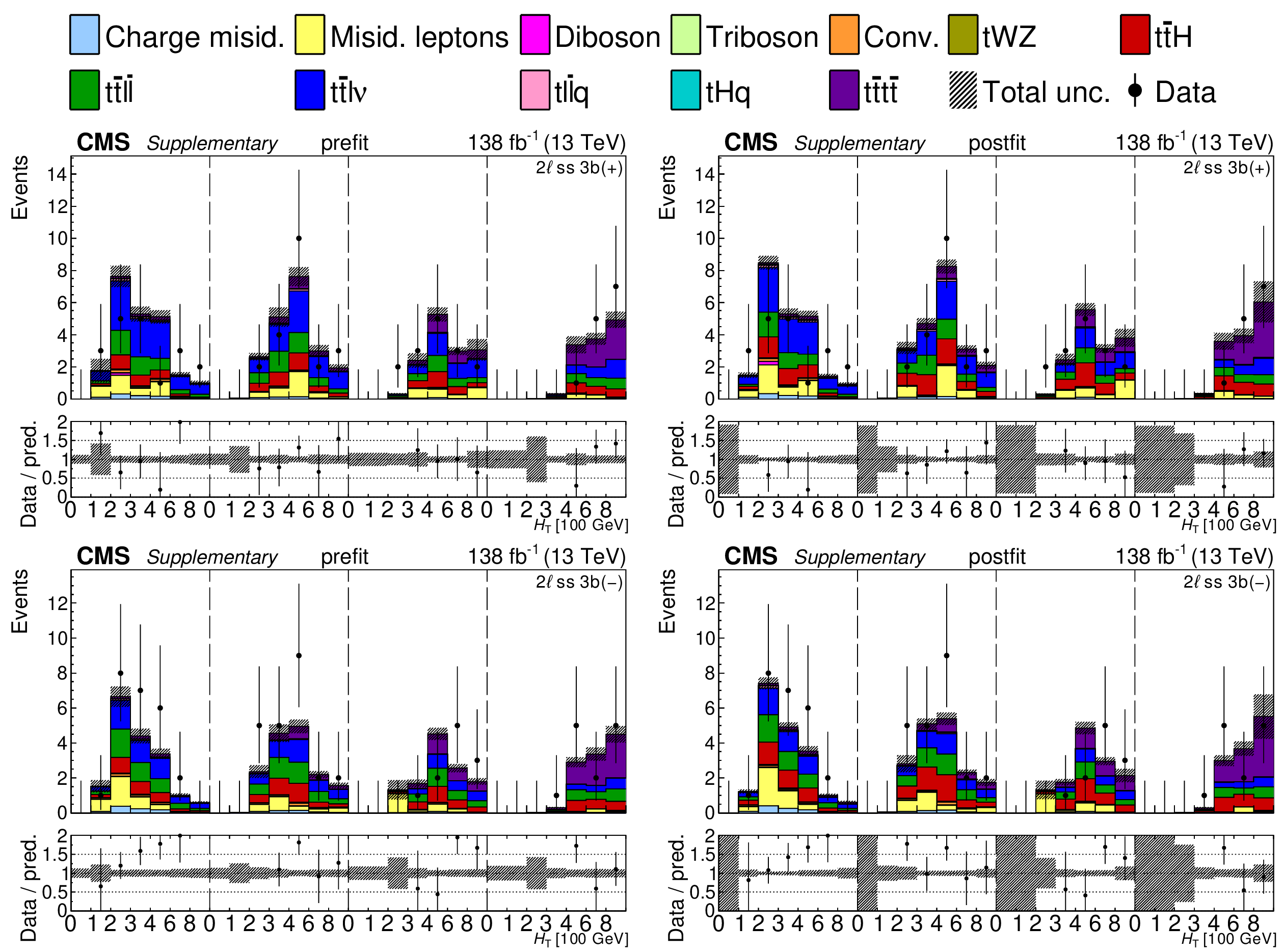
png pdf |
Additional Figure 31:
The top row shows the prefit (left) and postfit (right) yields of the channel 2$ \ell\text{ss 3b} \, (+) $. The bottom row shows the prefit (left) and postfit (right) yields of the channel 2$ \ell\text{ss 3b} \, (-) $. Multiple sets of prefit and postfit plots with the alternative kinematic distribution, including this set of $ H_{\mathrm{T}} $ plots, are used to check the effectiveness of the fit. The jet subcategories are arranged from low jet multiplicity to high jet multiplicity from left to right for each individual plot. For example, in the 2$ \ell\text{ss 3b} \, (+) $ plot, the first seven bins are the $ H_{\mathrm{T}} $ variable for 2$ \ell\text{ss 3b} \, (+) \: \mathrm{4j} $, the next seven bins are for 2$ \ell\text{ss 3b} \, (+) \: \mathrm{5j} $, etc. The process labeled ``Conv." corresponds to the photon conversion background, ``Misid. leptons" corresponds to misidentified leptons, and ``Charge misid." corresponds to leptons with a mismeasured charge. The lower panel contains the ratios of the observed yields over the expected. The error bands correspond to nuisance parameter and Wilson coefficient uncertainties added in quadrature. |

png pdf |
Additional Figure 31-a:
The top row shows the prefit (left) and postfit (right) yields of the channel 2$ \ell\text{ss 3b} \, (+) $. The bottom row shows the prefit (left) and postfit (right) yields of the channel 2$ \ell\text{ss 3b} \, (-) $. Multiple sets of prefit and postfit plots with the alternative kinematic distribution, including this set of $ H_{\mathrm{T}} $ plots, are used to check the effectiveness of the fit. The jet subcategories are arranged from low jet multiplicity to high jet multiplicity from left to right for each individual plot. For example, in the 2$ \ell\text{ss 3b} \, (+) $ plot, the first seven bins are the $ H_{\mathrm{T}} $ variable for 2$ \ell\text{ss 3b} \, (+) \: \mathrm{4j} $, the next seven bins are for 2$ \ell\text{ss 3b} \, (+) \: \mathrm{5j} $, etc. The process labeled ``Conv." corresponds to the photon conversion background, ``Misid. leptons" corresponds to misidentified leptons, and ``Charge misid." corresponds to leptons with a mismeasured charge. The lower panel contains the ratios of the observed yields over the expected. The error bands correspond to nuisance parameter and Wilson coefficient uncertainties added in quadrature. |

png pdf |
Additional Figure 31-b:
The top row shows the prefit (left) and postfit (right) yields of the channel 2$ \ell\text{ss 3b} \, (+) $. The bottom row shows the prefit (left) and postfit (right) yields of the channel 2$ \ell\text{ss 3b} \, (-) $. Multiple sets of prefit and postfit plots with the alternative kinematic distribution, including this set of $ H_{\mathrm{T}} $ plots, are used to check the effectiveness of the fit. The jet subcategories are arranged from low jet multiplicity to high jet multiplicity from left to right for each individual plot. For example, in the 2$ \ell\text{ss 3b} \, (+) $ plot, the first seven bins are the $ H_{\mathrm{T}} $ variable for 2$ \ell\text{ss 3b} \, (+) \: \mathrm{4j} $, the next seven bins are for 2$ \ell\text{ss 3b} \, (+) \: \mathrm{5j} $, etc. The process labeled ``Conv." corresponds to the photon conversion background, ``Misid. leptons" corresponds to misidentified leptons, and ``Charge misid." corresponds to leptons with a mismeasured charge. The lower panel contains the ratios of the observed yields over the expected. The error bands correspond to nuisance parameter and Wilson coefficient uncertainties added in quadrature. |

png pdf |
Additional Figure 31-c:
The top row shows the prefit (left) and postfit (right) yields of the channel 2$ \ell\text{ss 3b} \, (+) $. The bottom row shows the prefit (left) and postfit (right) yields of the channel 2$ \ell\text{ss 3b} \, (-) $. Multiple sets of prefit and postfit plots with the alternative kinematic distribution, including this set of $ H_{\mathrm{T}} $ plots, are used to check the effectiveness of the fit. The jet subcategories are arranged from low jet multiplicity to high jet multiplicity from left to right for each individual plot. For example, in the 2$ \ell\text{ss 3b} \, (+) $ plot, the first seven bins are the $ H_{\mathrm{T}} $ variable for 2$ \ell\text{ss 3b} \, (+) \: \mathrm{4j} $, the next seven bins are for 2$ \ell\text{ss 3b} \, (+) \: \mathrm{5j} $, etc. The process labeled ``Conv." corresponds to the photon conversion background, ``Misid. leptons" corresponds to misidentified leptons, and ``Charge misid." corresponds to leptons with a mismeasured charge. The lower panel contains the ratios of the observed yields over the expected. The error bands correspond to nuisance parameter and Wilson coefficient uncertainties added in quadrature. |

png pdf |
Additional Figure 31-d:
The top row shows the prefit (left) and postfit (right) yields of the channel 2$ \ell\text{ss 3b} \, (+) $. The bottom row shows the prefit (left) and postfit (right) yields of the channel 2$ \ell\text{ss 3b} \, (-) $. Multiple sets of prefit and postfit plots with the alternative kinematic distribution, including this set of $ H_{\mathrm{T}} $ plots, are used to check the effectiveness of the fit. The jet subcategories are arranged from low jet multiplicity to high jet multiplicity from left to right for each individual plot. For example, in the 2$ \ell\text{ss 3b} \, (+) $ plot, the first seven bins are the $ H_{\mathrm{T}} $ variable for 2$ \ell\text{ss 3b} \, (+) \: \mathrm{4j} $, the next seven bins are for 2$ \ell\text{ss 3b} \, (+) \: \mathrm{5j} $, etc. The process labeled ``Conv." corresponds to the photon conversion background, ``Misid. leptons" corresponds to misidentified leptons, and ``Charge misid." corresponds to leptons with a mismeasured charge. The lower panel contains the ratios of the observed yields over the expected. The error bands correspond to nuisance parameter and Wilson coefficient uncertainties added in quadrature. |

png pdf |
Additional Figure 31-e:
The top row shows the prefit (left) and postfit (right) yields of the channel 2$ \ell\text{ss 3b} \, (+) $. The bottom row shows the prefit (left) and postfit (right) yields of the channel 2$ \ell\text{ss 3b} \, (-) $. Multiple sets of prefit and postfit plots with the alternative kinematic distribution, including this set of $ H_{\mathrm{T}} $ plots, are used to check the effectiveness of the fit. The jet subcategories are arranged from low jet multiplicity to high jet multiplicity from left to right for each individual plot. For example, in the 2$ \ell\text{ss 3b} \, (+) $ plot, the first seven bins are the $ H_{\mathrm{T}} $ variable for 2$ \ell\text{ss 3b} \, (+) \: \mathrm{4j} $, the next seven bins are for 2$ \ell\text{ss 3b} \, (+) \: \mathrm{5j} $, etc. The process labeled ``Conv." corresponds to the photon conversion background, ``Misid. leptons" corresponds to misidentified leptons, and ``Charge misid." corresponds to leptons with a mismeasured charge. The lower panel contains the ratios of the observed yields over the expected. The error bands correspond to nuisance parameter and Wilson coefficient uncertainties added in quadrature. |

png pdf |
Additional Figure 32:
The top row shows the prefit (left) and postfit (right) yields of the channel 3$ \ell $ off-Z 1b $ (+) $. The bottom row shows the prefit (left) and postfit (right) yields of the channel 3$ \ell $ off-Z 1b $ (-) $. Multiple sets of prefit and postfit plots with the alternative kinematic distribution, including this set of $ H_{\mathrm{T}} $ plots, are used to check the effectiveness of the fit. The jet subcategories are arranged from low jet multiplicity to high jet multiplicity from left to right for each individual plot. For example, in the 3$ \ell $ off-Z 1b $ (+) $ plot, the first seven bins are the $ H_{\mathrm{T}} $ variable for 3$ \ell $ off-Z 1b $ (+) \: \mathrm{2j} $, the next seven bins are for 3$ \ell $ off-Z 1b $ (+) \: \mathrm{3j} $, etc. The process labeled ``Conv." corresponds to the photon conversion background, ``Misid. leptons" corresponds to misidentified leptons, and ``Charge misid." corresponds to leptons with a mismeasured charge. The lower panel contains the ratios of the observed yields over the expected. The error bands correspond to nuisance parameter and Wilson coefficient uncertainties added in quadrature. |

png pdf |
Additional Figure 32-a:
The top row shows the prefit (left) and postfit (right) yields of the channel 3$ \ell $ off-Z 1b $ (+) $. The bottom row shows the prefit (left) and postfit (right) yields of the channel 3$ \ell $ off-Z 1b $ (-) $. Multiple sets of prefit and postfit plots with the alternative kinematic distribution, including this set of $ H_{\mathrm{T}} $ plots, are used to check the effectiveness of the fit. The jet subcategories are arranged from low jet multiplicity to high jet multiplicity from left to right for each individual plot. For example, in the 3$ \ell $ off-Z 1b $ (+) $ plot, the first seven bins are the $ H_{\mathrm{T}} $ variable for 3$ \ell $ off-Z 1b $ (+) \: \mathrm{2j} $, the next seven bins are for 3$ \ell $ off-Z 1b $ (+) \: \mathrm{3j} $, etc. The process labeled ``Conv." corresponds to the photon conversion background, ``Misid. leptons" corresponds to misidentified leptons, and ``Charge misid." corresponds to leptons with a mismeasured charge. The lower panel contains the ratios of the observed yields over the expected. The error bands correspond to nuisance parameter and Wilson coefficient uncertainties added in quadrature. |

png pdf |
Additional Figure 32-b:
The top row shows the prefit (left) and postfit (right) yields of the channel 3$ \ell $ off-Z 1b $ (+) $. The bottom row shows the prefit (left) and postfit (right) yields of the channel 3$ \ell $ off-Z 1b $ (-) $. Multiple sets of prefit and postfit plots with the alternative kinematic distribution, including this set of $ H_{\mathrm{T}} $ plots, are used to check the effectiveness of the fit. The jet subcategories are arranged from low jet multiplicity to high jet multiplicity from left to right for each individual plot. For example, in the 3$ \ell $ off-Z 1b $ (+) $ plot, the first seven bins are the $ H_{\mathrm{T}} $ variable for 3$ \ell $ off-Z 1b $ (+) \: \mathrm{2j} $, the next seven bins are for 3$ \ell $ off-Z 1b $ (+) \: \mathrm{3j} $, etc. The process labeled ``Conv." corresponds to the photon conversion background, ``Misid. leptons" corresponds to misidentified leptons, and ``Charge misid." corresponds to leptons with a mismeasured charge. The lower panel contains the ratios of the observed yields over the expected. The error bands correspond to nuisance parameter and Wilson coefficient uncertainties added in quadrature. |

png pdf |
Additional Figure 32-c:
The top row shows the prefit (left) and postfit (right) yields of the channel 3$ \ell $ off-Z 1b $ (+) $. The bottom row shows the prefit (left) and postfit (right) yields of the channel 3$ \ell $ off-Z 1b $ (-) $. Multiple sets of prefit and postfit plots with the alternative kinematic distribution, including this set of $ H_{\mathrm{T}} $ plots, are used to check the effectiveness of the fit. The jet subcategories are arranged from low jet multiplicity to high jet multiplicity from left to right for each individual plot. For example, in the 3$ \ell $ off-Z 1b $ (+) $ plot, the first seven bins are the $ H_{\mathrm{T}} $ variable for 3$ \ell $ off-Z 1b $ (+) \: \mathrm{2j} $, the next seven bins are for 3$ \ell $ off-Z 1b $ (+) \: \mathrm{3j} $, etc. The process labeled ``Conv." corresponds to the photon conversion background, ``Misid. leptons" corresponds to misidentified leptons, and ``Charge misid." corresponds to leptons with a mismeasured charge. The lower panel contains the ratios of the observed yields over the expected. The error bands correspond to nuisance parameter and Wilson coefficient uncertainties added in quadrature. |

png pdf |
Additional Figure 32-d:
The top row shows the prefit (left) and postfit (right) yields of the channel 3$ \ell $ off-Z 1b $ (+) $. The bottom row shows the prefit (left) and postfit (right) yields of the channel 3$ \ell $ off-Z 1b $ (-) $. Multiple sets of prefit and postfit plots with the alternative kinematic distribution, including this set of $ H_{\mathrm{T}} $ plots, are used to check the effectiveness of the fit. The jet subcategories are arranged from low jet multiplicity to high jet multiplicity from left to right for each individual plot. For example, in the 3$ \ell $ off-Z 1b $ (+) $ plot, the first seven bins are the $ H_{\mathrm{T}} $ variable for 3$ \ell $ off-Z 1b $ (+) \: \mathrm{2j} $, the next seven bins are for 3$ \ell $ off-Z 1b $ (+) \: \mathrm{3j} $, etc. The process labeled ``Conv." corresponds to the photon conversion background, ``Misid. leptons" corresponds to misidentified leptons, and ``Charge misid." corresponds to leptons with a mismeasured charge. The lower panel contains the ratios of the observed yields over the expected. The error bands correspond to nuisance parameter and Wilson coefficient uncertainties added in quadrature. |

png pdf |
Additional Figure 32-e:
The top row shows the prefit (left) and postfit (right) yields of the channel 3$ \ell $ off-Z 1b $ (+) $. The bottom row shows the prefit (left) and postfit (right) yields of the channel 3$ \ell $ off-Z 1b $ (-) $. Multiple sets of prefit and postfit plots with the alternative kinematic distribution, including this set of $ H_{\mathrm{T}} $ plots, are used to check the effectiveness of the fit. The jet subcategories are arranged from low jet multiplicity to high jet multiplicity from left to right for each individual plot. For example, in the 3$ \ell $ off-Z 1b $ (+) $ plot, the first seven bins are the $ H_{\mathrm{T}} $ variable for 3$ \ell $ off-Z 1b $ (+) \: \mathrm{2j} $, the next seven bins are for 3$ \ell $ off-Z 1b $ (+) \: \mathrm{3j} $, etc. The process labeled ``Conv." corresponds to the photon conversion background, ``Misid. leptons" corresponds to misidentified leptons, and ``Charge misid." corresponds to leptons with a mismeasured charge. The lower panel contains the ratios of the observed yields over the expected. The error bands correspond to nuisance parameter and Wilson coefficient uncertainties added in quadrature. |

png pdf |
Additional Figure 33:
The top row shows the prefit (left) and postfit (right) yields of the channel 3$ \ell $ off-Z 2b $ (+) $. The bottom row shows the prefit (left) and postfit (right) yields of the channel 3$ \ell $ off-Z 2b $ (-) $. Multiple sets of prefit and postfit plots with the alternative kinematic distribution, including this set of $ H_{\mathrm{T}} $ plots, are used to check the effectiveness of the fit. The jet subcategories are arranged from low jet multiplicity to high jet multiplicity from left to right for each individual plot. For example, in the 3$ \ell $ off-Z 2b $ (+) $ plot, the first seven bins are the $ H_{\mathrm{T}} $ variable for 3$ \ell $ off-Z 2b $ (+) \: \mathrm{2j} $, the next seven bins are for 3$ \ell $ off-Z 2b $ (+) \: \mathrm{3j} $, etc. The process labeled ``Conv." corresponds to the photon conversion background, ``Misid. leptons" corresponds to misidentified leptons, and ``Charge misid." corresponds to leptons with a mismeasured charge. The lower panel contains the ratios of the observed yields over the expected. The error bands correspond to nuisance parameter and Wilson coefficient uncertainties added in quadrature. |

png pdf |
Additional Figure 33-a:
The top row shows the prefit (left) and postfit (right) yields of the channel 3$ \ell $ off-Z 2b $ (+) $. The bottom row shows the prefit (left) and postfit (right) yields of the channel 3$ \ell $ off-Z 2b $ (-) $. Multiple sets of prefit and postfit plots with the alternative kinematic distribution, including this set of $ H_{\mathrm{T}} $ plots, are used to check the effectiveness of the fit. The jet subcategories are arranged from low jet multiplicity to high jet multiplicity from left to right for each individual plot. For example, in the 3$ \ell $ off-Z 2b $ (+) $ plot, the first seven bins are the $ H_{\mathrm{T}} $ variable for 3$ \ell $ off-Z 2b $ (+) \: \mathrm{2j} $, the next seven bins are for 3$ \ell $ off-Z 2b $ (+) \: \mathrm{3j} $, etc. The process labeled ``Conv." corresponds to the photon conversion background, ``Misid. leptons" corresponds to misidentified leptons, and ``Charge misid." corresponds to leptons with a mismeasured charge. The lower panel contains the ratios of the observed yields over the expected. The error bands correspond to nuisance parameter and Wilson coefficient uncertainties added in quadrature. |

png pdf |
Additional Figure 33-b:
The top row shows the prefit (left) and postfit (right) yields of the channel 3$ \ell $ off-Z 2b $ (+) $. The bottom row shows the prefit (left) and postfit (right) yields of the channel 3$ \ell $ off-Z 2b $ (-) $. Multiple sets of prefit and postfit plots with the alternative kinematic distribution, including this set of $ H_{\mathrm{T}} $ plots, are used to check the effectiveness of the fit. The jet subcategories are arranged from low jet multiplicity to high jet multiplicity from left to right for each individual plot. For example, in the 3$ \ell $ off-Z 2b $ (+) $ plot, the first seven bins are the $ H_{\mathrm{T}} $ variable for 3$ \ell $ off-Z 2b $ (+) \: \mathrm{2j} $, the next seven bins are for 3$ \ell $ off-Z 2b $ (+) \: \mathrm{3j} $, etc. The process labeled ``Conv." corresponds to the photon conversion background, ``Misid. leptons" corresponds to misidentified leptons, and ``Charge misid." corresponds to leptons with a mismeasured charge. The lower panel contains the ratios of the observed yields over the expected. The error bands correspond to nuisance parameter and Wilson coefficient uncertainties added in quadrature. |

png pdf |
Additional Figure 33-c:
The top row shows the prefit (left) and postfit (right) yields of the channel 3$ \ell $ off-Z 2b $ (+) $. The bottom row shows the prefit (left) and postfit (right) yields of the channel 3$ \ell $ off-Z 2b $ (-) $. Multiple sets of prefit and postfit plots with the alternative kinematic distribution, including this set of $ H_{\mathrm{T}} $ plots, are used to check the effectiveness of the fit. The jet subcategories are arranged from low jet multiplicity to high jet multiplicity from left to right for each individual plot. For example, in the 3$ \ell $ off-Z 2b $ (+) $ plot, the first seven bins are the $ H_{\mathrm{T}} $ variable for 3$ \ell $ off-Z 2b $ (+) \: \mathrm{2j} $, the next seven bins are for 3$ \ell $ off-Z 2b $ (+) \: \mathrm{3j} $, etc. The process labeled ``Conv." corresponds to the photon conversion background, ``Misid. leptons" corresponds to misidentified leptons, and ``Charge misid." corresponds to leptons with a mismeasured charge. The lower panel contains the ratios of the observed yields over the expected. The error bands correspond to nuisance parameter and Wilson coefficient uncertainties added in quadrature. |

png pdf |
Additional Figure 33-d:
The top row shows the prefit (left) and postfit (right) yields of the channel 3$ \ell $ off-Z 2b $ (+) $. The bottom row shows the prefit (left) and postfit (right) yields of the channel 3$ \ell $ off-Z 2b $ (-) $. Multiple sets of prefit and postfit plots with the alternative kinematic distribution, including this set of $ H_{\mathrm{T}} $ plots, are used to check the effectiveness of the fit. The jet subcategories are arranged from low jet multiplicity to high jet multiplicity from left to right for each individual plot. For example, in the 3$ \ell $ off-Z 2b $ (+) $ plot, the first seven bins are the $ H_{\mathrm{T}} $ variable for 3$ \ell $ off-Z 2b $ (+) \: \mathrm{2j} $, the next seven bins are for 3$ \ell $ off-Z 2b $ (+) \: \mathrm{3j} $, etc. The process labeled ``Conv." corresponds to the photon conversion background, ``Misid. leptons" corresponds to misidentified leptons, and ``Charge misid." corresponds to leptons with a mismeasured charge. The lower panel contains the ratios of the observed yields over the expected. The error bands correspond to nuisance parameter and Wilson coefficient uncertainties added in quadrature. |

png pdf |
Additional Figure 33-e:
The top row shows the prefit (left) and postfit (right) yields of the channel 3$ \ell $ off-Z 2b $ (+) $. The bottom row shows the prefit (left) and postfit (right) yields of the channel 3$ \ell $ off-Z 2b $ (-) $. Multiple sets of prefit and postfit plots with the alternative kinematic distribution, including this set of $ H_{\mathrm{T}} $ plots, are used to check the effectiveness of the fit. The jet subcategories are arranged from low jet multiplicity to high jet multiplicity from left to right for each individual plot. For example, in the 3$ \ell $ off-Z 2b $ (+) $ plot, the first seven bins are the $ H_{\mathrm{T}} $ variable for 3$ \ell $ off-Z 2b $ (+) \: \mathrm{2j} $, the next seven bins are for 3$ \ell $ off-Z 2b $ (+) \: \mathrm{3j} $, etc. The process labeled ``Conv." corresponds to the photon conversion background, ``Misid. leptons" corresponds to misidentified leptons, and ``Charge misid." corresponds to leptons with a mismeasured charge. The lower panel contains the ratios of the observed yields over the expected. The error bands correspond to nuisance parameter and Wilson coefficient uncertainties added in quadrature. |

png pdf |
Additional Figure 34:
The top row shows the prefit (left) and postfit (right) yields of the channel 3$ \ell $ on-Z 1b. The bottom row shows the prefit (left) and postfit (right) yields of the channel 3$ \ell $ on-Z 2b. Multiple sets of prefit and postfit plots with the alternative kinematic distribution, including this set of $ H_{\mathrm{T}} $ plots, are used to check the effectiveness of the fit. The jet subcategories are arranged from low jet multiplicity to high jet multiplicity from left to right for each individual plot. For example, in the 3$ \ell $ on-Z 1b plot, the first seven bins are the $ H_{\mathrm{T}} $ variable for 3$ \ell $ on-Z 1b $ \mathrm{2j} $, the next seven bins are for 3$ \ell $ on-Z 1b $ \mathrm{3j} $, etc. The process labeled ``Conv." corresponds to the photon conversion background, ``Misid. leptons" corresponds to misidentified leptons, and ``Charge misid." corresponds to leptons with a mismeasured charge. The lower panel contains the ratios of the observed yields over the expected. The error bands correspond to nuisance parameter and Wilson coefficient uncertainties added in quadrature. |

png pdf |
Additional Figure 34-a:
The top row shows the prefit (left) and postfit (right) yields of the channel 3$ \ell $ on-Z 1b. The bottom row shows the prefit (left) and postfit (right) yields of the channel 3$ \ell $ on-Z 2b. Multiple sets of prefit and postfit plots with the alternative kinematic distribution, including this set of $ H_{\mathrm{T}} $ plots, are used to check the effectiveness of the fit. The jet subcategories are arranged from low jet multiplicity to high jet multiplicity from left to right for each individual plot. For example, in the 3$ \ell $ on-Z 1b plot, the first seven bins are the $ H_{\mathrm{T}} $ variable for 3$ \ell $ on-Z 1b $ \mathrm{2j} $, the next seven bins are for 3$ \ell $ on-Z 1b $ \mathrm{3j} $, etc. The process labeled ``Conv." corresponds to the photon conversion background, ``Misid. leptons" corresponds to misidentified leptons, and ``Charge misid." corresponds to leptons with a mismeasured charge. The lower panel contains the ratios of the observed yields over the expected. The error bands correspond to nuisance parameter and Wilson coefficient uncertainties added in quadrature. |
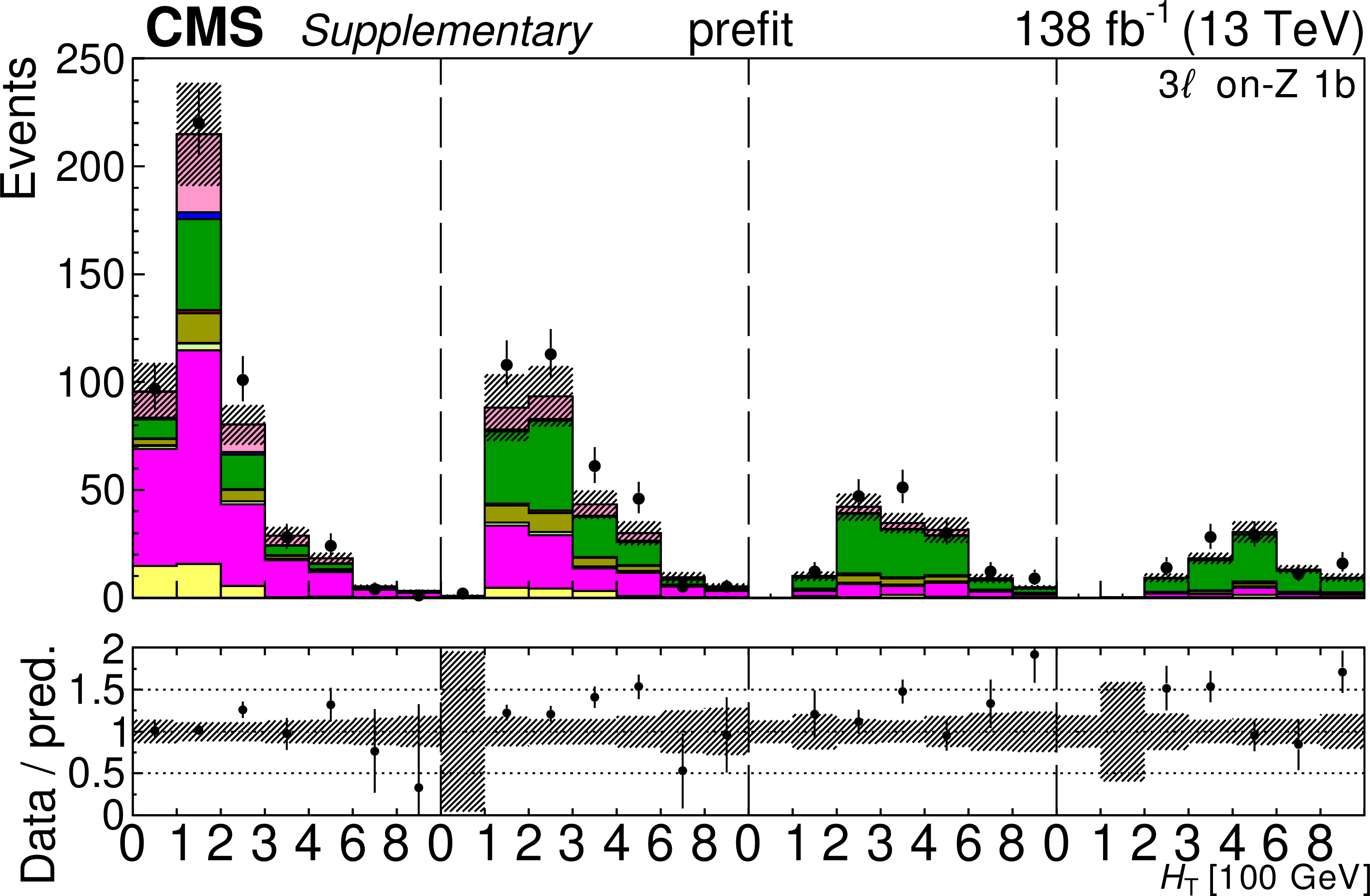
png pdf |
Additional Figure 34-b:
The top row shows the prefit (left) and postfit (right) yields of the channel 3$ \ell $ on-Z 1b. The bottom row shows the prefit (left) and postfit (right) yields of the channel 3$ \ell $ on-Z 2b. Multiple sets of prefit and postfit plots with the alternative kinematic distribution, including this set of $ H_{\mathrm{T}} $ plots, are used to check the effectiveness of the fit. The jet subcategories are arranged from low jet multiplicity to high jet multiplicity from left to right for each individual plot. For example, in the 3$ \ell $ on-Z 1b plot, the first seven bins are the $ H_{\mathrm{T}} $ variable for 3$ \ell $ on-Z 1b $ \mathrm{2j} $, the next seven bins are for 3$ \ell $ on-Z 1b $ \mathrm{3j} $, etc. The process labeled ``Conv." corresponds to the photon conversion background, ``Misid. leptons" corresponds to misidentified leptons, and ``Charge misid." corresponds to leptons with a mismeasured charge. The lower panel contains the ratios of the observed yields over the expected. The error bands correspond to nuisance parameter and Wilson coefficient uncertainties added in quadrature. |

png pdf |
Additional Figure 34-c:
The top row shows the prefit (left) and postfit (right) yields of the channel 3$ \ell $ on-Z 1b. The bottom row shows the prefit (left) and postfit (right) yields of the channel 3$ \ell $ on-Z 2b. Multiple sets of prefit and postfit plots with the alternative kinematic distribution, including this set of $ H_{\mathrm{T}} $ plots, are used to check the effectiveness of the fit. The jet subcategories are arranged from low jet multiplicity to high jet multiplicity from left to right for each individual plot. For example, in the 3$ \ell $ on-Z 1b plot, the first seven bins are the $ H_{\mathrm{T}} $ variable for 3$ \ell $ on-Z 1b $ \mathrm{2j} $, the next seven bins are for 3$ \ell $ on-Z 1b $ \mathrm{3j} $, etc. The process labeled ``Conv." corresponds to the photon conversion background, ``Misid. leptons" corresponds to misidentified leptons, and ``Charge misid." corresponds to leptons with a mismeasured charge. The lower panel contains the ratios of the observed yields over the expected. The error bands correspond to nuisance parameter and Wilson coefficient uncertainties added in quadrature. |

png pdf |
Additional Figure 34-d:
The top row shows the prefit (left) and postfit (right) yields of the channel 3$ \ell $ on-Z 1b. The bottom row shows the prefit (left) and postfit (right) yields of the channel 3$ \ell $ on-Z 2b. Multiple sets of prefit and postfit plots with the alternative kinematic distribution, including this set of $ H_{\mathrm{T}} $ plots, are used to check the effectiveness of the fit. The jet subcategories are arranged from low jet multiplicity to high jet multiplicity from left to right for each individual plot. For example, in the 3$ \ell $ on-Z 1b plot, the first seven bins are the $ H_{\mathrm{T}} $ variable for 3$ \ell $ on-Z 1b $ \mathrm{2j} $, the next seven bins are for 3$ \ell $ on-Z 1b $ \mathrm{3j} $, etc. The process labeled ``Conv." corresponds to the photon conversion background, ``Misid. leptons" corresponds to misidentified leptons, and ``Charge misid." corresponds to leptons with a mismeasured charge. The lower panel contains the ratios of the observed yields over the expected. The error bands correspond to nuisance parameter and Wilson coefficient uncertainties added in quadrature. |
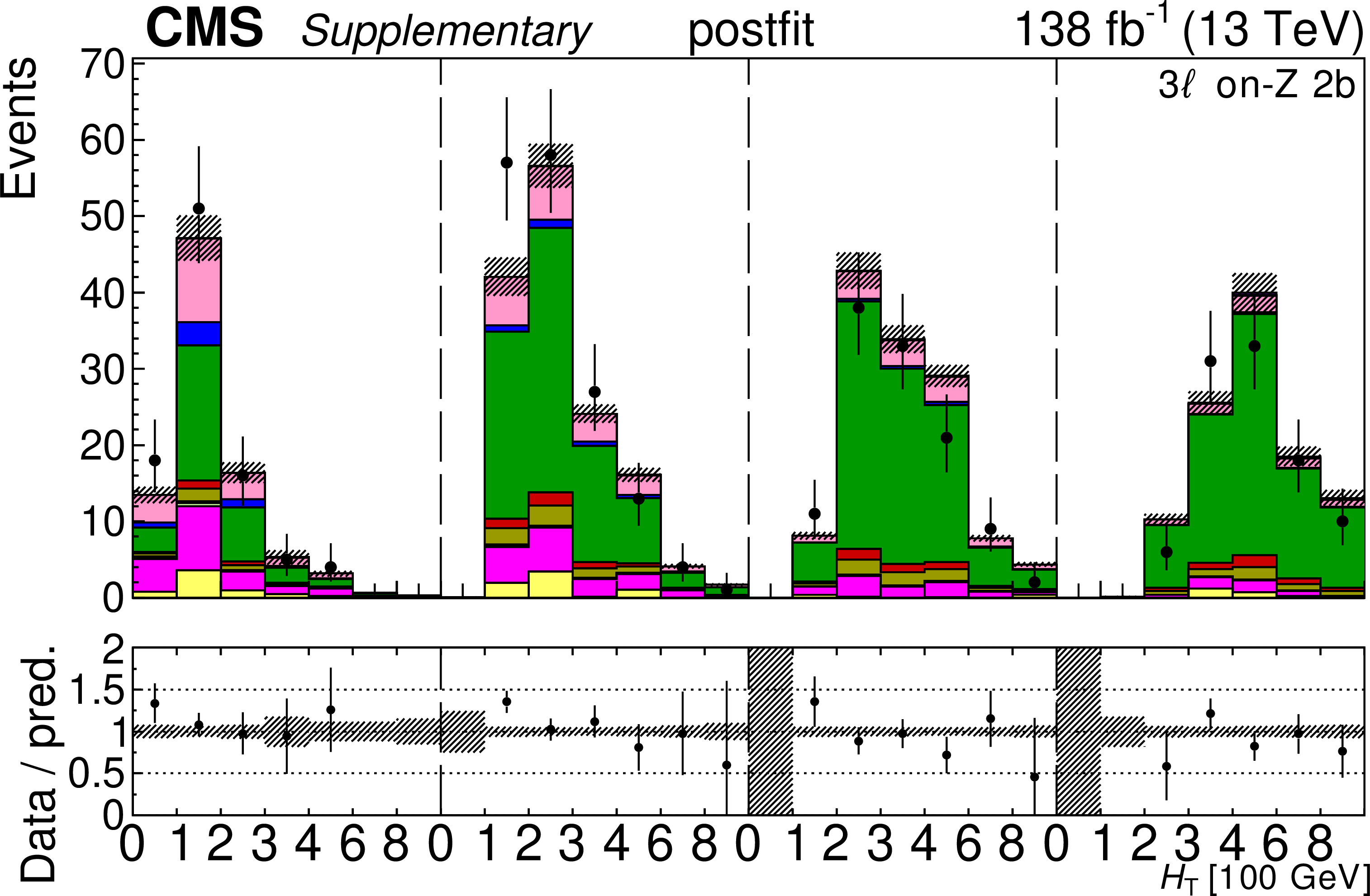
png pdf |
Additional Figure 34-e:
The top row shows the prefit (left) and postfit (right) yields of the channel 3$ \ell $ on-Z 1b. The bottom row shows the prefit (left) and postfit (right) yields of the channel 3$ \ell $ on-Z 2b. Multiple sets of prefit and postfit plots with the alternative kinematic distribution, including this set of $ H_{\mathrm{T}} $ plots, are used to check the effectiveness of the fit. The jet subcategories are arranged from low jet multiplicity to high jet multiplicity from left to right for each individual plot. For example, in the 3$ \ell $ on-Z 1b plot, the first seven bins are the $ H_{\mathrm{T}} $ variable for 3$ \ell $ on-Z 1b $ \mathrm{2j} $, the next seven bins are for 3$ \ell $ on-Z 1b $ \mathrm{3j} $, etc. The process labeled ``Conv." corresponds to the photon conversion background, ``Misid. leptons" corresponds to misidentified leptons, and ``Charge misid." corresponds to leptons with a mismeasured charge. The lower panel contains the ratios of the observed yields over the expected. The error bands correspond to nuisance parameter and Wilson coefficient uncertainties added in quadrature. |

png pdf |
Additional Figure 35:
Prefit (left) and postfit (right) yields of the channel 4$ \ell $. Multiple sets of prefit and postfit plots with the alternative kinematic distribution, including this set of $ H_{\mathrm{T}} $ plots, are used to check the effectiveness of the fit. The jet subcategories are arranged from low jet multiplicity to high jet multiplicity from left to right for each individual plot. In the 4$ \ell $ plot, the first seven bins are the $ H_{\mathrm{T}} $ variable for 4$ \ell \mathrm{2j} $, the next seven bins are for 4$ \ell \mathrm{3j} $, etc. The process labeled ``Conv." corresponds to the photon conversion background, ``Misid. leptons" corresponds to misidentified leptons, and ``Charge misid." corresponds to leptons with a mismeasured charge. The lower panel contains the ratios of the observed yields over the expected. The error bands correspond to nuisance parameter and Wilson coefficient uncertainties added in quadrature. |

png pdf |
Additional Figure 35-a:
Prefit (left) and postfit (right) yields of the channel 4$ \ell $. Multiple sets of prefit and postfit plots with the alternative kinematic distribution, including this set of $ H_{\mathrm{T}} $ plots, are used to check the effectiveness of the fit. The jet subcategories are arranged from low jet multiplicity to high jet multiplicity from left to right for each individual plot. In the 4$ \ell $ plot, the first seven bins are the $ H_{\mathrm{T}} $ variable for 4$ \ell \mathrm{2j} $, the next seven bins are for 4$ \ell \mathrm{3j} $, etc. The process labeled ``Conv." corresponds to the photon conversion background, ``Misid. leptons" corresponds to misidentified leptons, and ``Charge misid." corresponds to leptons with a mismeasured charge. The lower panel contains the ratios of the observed yields over the expected. The error bands correspond to nuisance parameter and Wilson coefficient uncertainties added in quadrature. |

png pdf |
Additional Figure 35-b:
Prefit (left) and postfit (right) yields of the channel 4$ \ell $. Multiple sets of prefit and postfit plots with the alternative kinematic distribution, including this set of $ H_{\mathrm{T}} $ plots, are used to check the effectiveness of the fit. The jet subcategories are arranged from low jet multiplicity to high jet multiplicity from left to right for each individual plot. In the 4$ \ell $ plot, the first seven bins are the $ H_{\mathrm{T}} $ variable for 4$ \ell \mathrm{2j} $, the next seven bins are for 4$ \ell \mathrm{3j} $, etc. The process labeled ``Conv." corresponds to the photon conversion background, ``Misid. leptons" corresponds to misidentified leptons, and ``Charge misid." corresponds to leptons with a mismeasured charge. The lower panel contains the ratios of the observed yields over the expected. The error bands correspond to nuisance parameter and Wilson coefficient uncertainties added in quadrature. |

png pdf |
Additional Figure 35-c:
Prefit (left) and postfit (right) yields of the channel 4$ \ell $. Multiple sets of prefit and postfit plots with the alternative kinematic distribution, including this set of $ H_{\mathrm{T}} $ plots, are used to check the effectiveness of the fit. The jet subcategories are arranged from low jet multiplicity to high jet multiplicity from left to right for each individual plot. In the 4$ \ell $ plot, the first seven bins are the $ H_{\mathrm{T}} $ variable for 4$ \ell \mathrm{2j} $, the next seven bins are for 4$ \ell \mathrm{3j} $, etc. The process labeled ``Conv." corresponds to the photon conversion background, ``Misid. leptons" corresponds to misidentified leptons, and ``Charge misid." corresponds to leptons with a mismeasured charge. The lower panel contains the ratios of the observed yields over the expected. The error bands correspond to nuisance parameter and Wilson coefficient uncertainties added in quadrature. |
| References | ||||
| 1 | J. L. Feng | Dark matter candidates from particle physics and methods of detection | Ann. Rev. Astron. Astrophys. 48 (2010) 495 | 1003.0904 |
| 2 | T. A. Porter, R. P. Johnson, and P. W. Graham | Dark matter searches with astroparticle data | Ann. Rev. Astron. Astrophys. 49 (2011) 155 | 1104.2836 |
| 3 | C. Degrande et al. | Effective field theory: A modern approach to anomalous couplings | Annals Phys. 335 (2013) 21 | 1205.4231 |
| 4 | CDF Collaboration | Observation of top quark production in $ {\overline{\mathrm{p}}\mathrm{p}} $ collisions | PRL 74 (1995) 2626 | hep-ex/9503002 |
| 5 | \DZERO Collaboration | Observation of the top quark | PRL 74 (1995) 2632 | hep-ex/9503003 |
| 6 | Particle Data Group, R. L. Workman et al. | Review of particle physics | Prog. Theor. Exp. Phys. 2022 (2022) 083C01 | |
| 7 | CMS Collaboration | Measurement of the Higgs boson production rate in association with top quarks in final states with electrons, muons, and hadronically decaying tau leptons at $ \sqrt{s}= $ 13 TeV | EPJC 81 (2021) 378 | CMS-HIG-19-008 2011.03652 |
| 8 | CMS Collaboration | Measurement of the cross section of top quark-antiquark pair production in association with a W boson in proton-proton collisions at $ \sqrt{s}= $ 13 TeV | Accepted by JHEP, 2022 | CMS-TOP-21-011 2208.06485 |
| 9 | CMS Collaboration | Measurement of top quark pair production in association with a Z boson in proton-proton collisions at $ \sqrt{s}= $ 13 TeV | JHEP 03 (2020) 056 | CMS-TOP-18-009 1907.11270 |
| 10 | CMS Collaboration | Inclusive and differential cross section measurements of single top quark production in association with a Z boson in proton-proton collisions at $ \sqrt{s}= $ 13 TeV | JHEP 02 (2022) 107 | CMS-TOP-20-010 2111.02860 |
| 11 | CMS Collaboration | Evidence for four-top quark production in proton-proton collisions at $ \sqrt{s}= $ 13 TeV | Accepted by PLB, 2023 | CMS-TOP-21-005 2303.03864 |
| 12 | CMS Collaboration | Search for new physics in top quark production with additional leptons in proton-proton collisions at $ \sqrt{s}= $ 13 TeV using effective field theory | JHEP 03 (2021) 095 | CMS-TOP-19-001 2012.04120 |
| 13 | CMS Collaboration | Probing effective field theory operators in the associated production of top quarks with a Z boson in multilepton final states at $ \sqrt{s}= $ 13 TeV | JHEP 12 (2021) 083 | CMS-TOP-21-001 2107.13896 |
| 14 | CMS Collaboration | Search for new physics using effective field theory in 13 TeV $ {\mathrm{p}\mathrm{p}} $ collision events that contain a top quark pair and a boosted Z or Higgs boson | Accepted by PRD, 2022 | CMS-TOP-21-003 2208.12837 |
| 15 | CMS Collaboration | HEPData record for this analysis | link | |
| 16 | CMS Collaboration | The CMS experiment at the CERN LHC | JINST 3 (2008) S08004 | |
| 17 | CMS Collaboration | Performance of the CMS Level-1 trigger in proton-proton collisions at $ \sqrt{s}= $ 13 TeV | JINST 15 (2020) P10017 | CMS-TRG-17-001 2006.10165 |
| 18 | CMS Collaboration | The CMS trigger system | JINST 12 (2017) P01020 | CMS-TRG-12-001 1609.02366 |
| 19 | J. Alwall et al. | The automated computation of tree-level and next-to-leading order differential cross sections, and their matching to parton shower simulations | JHEP 07 (2014) 079 | 1405.0301 |
| 20 | R. Frederix and S. Frixione | Merging meets matching in MC@NLO | JHEP 12 (2012) 061 | 1209.6215 |
| 21 | J. Alwall et al. | Comparative study of various algorithms for the merging of parton showers and matrix elements in hadronic collisions | EPJC 53 (2008) 473 | 0706.2569 |
| 22 | J. A. Aguilar-Saavedra et al. | Interpreting top-quark LHC measurements in the standard-model effective field theory | LHC TOP WG note CERN-LPCC-2018-01, 2018 | 1802.07237 |
| 23 | B. Grzadkowski, M. Iskrzynski, M. Misiak, and J. Rosiek | Dimension-six terms in the standard model Lagrangian | JHEP 10 (2010) 085 | 1008.4884 |
| 24 | R. Goldouzian et al. | Matching in $ {\mathrm{p}\mathrm{p}\to{\mathrm{t}\overline{\mathrm{t}}} \mathrm{W}/\mathrm{Z}/\mathrm{h}} $+jet SMEFT studies | JHEP 06 (2021) 151 | 2012.06872 |
| 25 | NNPDF Collaboration | Parton distributions for the LHC run II | JHEP 04 (2015) 040 | 1410.8849 |
| 26 | T. Sjöstrand, S. Mrenna, and P. Z. Skands | A brief introduction to PYTHIA8.1 | Comput. Phys. Commun. 178 (2008) 852 | 0710.3820 |
| 27 | CMS Collaboration | Extraction and validation of a new set of CMS PYTHIA8 tunes from underlying-event measurements | EPJC 80 (2020) 4 | CMS-GEN-17-001 1903.12179 |
| 28 | LHC Higgs Cross Section Working Group , D. de Florian et al. | Handbook of LHC Higgs cross sections: 4. Deciphering the nature of the Higgs sector | CERN Report CERN-2017-002-M, 2016 link |
1610.07922 |
| 29 | R. Frederix and I. Tsinikos | On improving NLO merging for $ {{\mathrm{t}\overline{\mathrm{t}}} \mathrm{W}} $ production | JHEP 11 (2021) 029 | 2108.07826 |
| 30 | M. van Beekveld, A. Kulesza, and L. M. Valero | Threshold resummation for the production of four top quarks at the LHC | 2212.03259 | |
| 31 | O. Mattelaer | On the maximal use of Monte Carlo samples: re-weighting events at NLO accuracy | EPJC 76 (2016) 674 | 1607.00763 |
| 32 | CMS Collaboration | Particle-flow reconstruction and global event description with the CMS detector | JINST 12 (2017) P10003 | CMS-PRF-14-001 1706.04965 |
| 33 | CMS Collaboration | Electron and photon reconstruction and identification with the CMS experiment at the CERN LHC | JINST 16 (2021) P05014 | CMS-EGM-17-001 2012.06888 |
| 34 | CMS Collaboration | ECAL 2016 refined calibration and Run2 summary plots | CMS Detector Performance Note CMS-DP-2020-021, 2020 CDS |
|
| 35 | CMS Collaboration | Performance of the CMS muon detector and muon reconstruction with proton-proton collisions at $ \sqrt{s}= $ 13 TeV | JINST 13 (2018) P06015 | CMS-MUO-16-001 1804.04528 |
| 36 | CMS Collaboration | Identification of prompt and isolated muons using multivariate techniques at the CMS experiment in proton-proton collisions at $ \sqrt{s}= $ 13 TeV | CMS Physics Analysis Summary, 2023 CMS-PAS-MUO-22-001 |
CMS-PAS-MUO-22-001 |
| 37 | M. Cacciari, G. P. Salam, and G. Soyez | The anti-$ k_{\mathrm{T}} $ jet clustering algorithm | JHEP 04 (2008) 063 | 0802.1189 |
| 38 | M. Cacciari, G. P. Salam, and G. Soyez | FASTJET user manual | EPJC 72 (2012) 1896 | 1111.6097 |
| 39 | CMS Collaboration | Pileup mitigation at CMS in 13 TeV data | JINST 15 (2020) P09018 | CMS-JME-18-001 2003.00503 |
| 40 | CMS Collaboration | Jet energy scale and resolution in the CMS experiment in $ {\mathrm{p}\mathrm{p}} $ collisions at 8 TeV | JINST 12 (2017) P02014 | CMS-JME-13-004 1607.03663 |
| 41 | CMS Collaboration | Identification of heavy-flavour jets with the CMS detector in $ {\mathrm{p}\mathrm{p}} $ collisions at 13 TeV | JINST 13 (2018) P05011 | CMS-BTV-16-002 1712.07158 |
| 42 | E. Bols et al. | Jet flavour classification using DEEPJET | JINST 15 (2020) P12012 | 2008.10519 |
| 43 | CMS Collaboration | Performance summary of AK4 jet b tagging with data from proton-proton collisions at 13 TeV with the CMS detector | CMS Detector Performance Note CMS-DP-2023-005, 2023 CDS |
|
| 44 | P. Nason | A new method for combining NLO QCD with shower Monte Carlo algorithms | JHEP 11 (2004) 040 | hep-ph/0409146 |
| 45 | S. Frixione, P. Nason, and C. Oleari | Matching NLO QCD computations with parton shower simulations: the POWHEG method | JHEP 11 (2007) 070 | 0709.2092 |
| 46 | S. Alioli, P. Nason, C. Oleari, and E. Re | A general framework for implementing NLO calculations in shower Monte Carlo programs: the POWHEG \textscbox | JHEP 06 (2010) 043 | 1002.2581 |
| 47 | T. Melia, P. Nason, R. Rontsch, and G. Zanderighi | $ {\mathrm{W^+}\mathrm{W^-}} $, $ {\mathrm{W}\mathrm{Z}} $ and $ {\mathrm{Z}\mathrm{Z}} $ production in the POWHEG \textscbox | JHEP 11 (2011) 078 | 1107.5051 |
| 48 | S. Frixione, G. Ridolfi, and P. Nason | A positive-weight next-to-leading-order Monte Carlo for heavy flavour hadroproduction | JHEP 09 (2007) 126 | 0707.3088 |
| 49 | J. M. Campbell and R. K. Ellis | An update on vector boson pair production at hadron colliders | PRD 60 (1999) 113006 | hep-ph/9905386 |
| 50 | M. Grazzini et al. | NNLO QCD + NLO EW with \textscMatrix+\textscOpenLoops: precise predictions for vector-boson pair production | JHEP 02 (2020) 087 | 1912.00068 |
| 51 | F. Caola, K. Melnikov, R. Röntsch, and L. Tancredi | QCD corrections to $ {\mathrm{Z}\mathrm{Z}} $ production in gluon fusion at the LHC | PRD 92 (2015) 094028 | 1509.06734 |
| 52 | CMS Collaboration | Search for electroweak production of charginos and neutralinos in multilepton final states in proton-proton collisions at $ \sqrt{s}= $ 13 TeV | JHEP 03 (2018) 166 | CMS-SUS-16-039 1709.05406 |
| 53 | W. Verkerke and D. Kirkby | The RooFit toolkit for data modeling | in 13th Int. Conf. on Computing in High Energy and Nuclear Phys. (CHEP ): La Jolla CA, USA, 2003 Proc. 1 (2003) 3 |
physics/0306116 |
| 54 | CMS Collaboration | Precision luminosity measurement in proton-proton collisions at $ \sqrt{s}= $ 13 TeV in 2015 and 2016 at CMS | EPJC 81 (2021) 800 | CMS-LUM-17-003 2104.01927 |
| 55 | CMS Collaboration | CMS luminosity measurement for the 2017 data-taking period at $ \sqrt{s}= $ 13 TeV | CMS Physics Analysis Summary, 2018 CMS-PAS-LUM-17-004 |
CMS-PAS-LUM-17-004 |
| 56 | CMS Collaboration | CMS luminosity measurement for the 2018 data-taking period at $ \sqrt{s}= $ 13 TeV | CMS Physics Analysis Summary, 2019 CMS-PAS-LUM-18-002 |
CMS-PAS-LUM-18-002 |
| 57 | CMS Collaboration | Measurements of inclusive W and Z cross sections in $ {\mathrm{p}\mathrm{p}} $ collisions at $ \sqrt{s}= $ 7 TeV | JHEP 01 (2011) 080 | CMS-EWK-10-002 1012.2466 |
| 58 | CMS Collaboration | Measurement of the inelastic proton-proton cross section at $ \sqrt{s}= $ 13 TeV | JHEP 07 (2018) 161 | CMS-FSQ-15-005 1802.02613 |
| 59 | J. Butterworth et al. | PDF4LHC recommendations for LHC Run II | JPG 43 (2016) 023001 | 1510.03865 |
|
|
Compact Muon Solenoid LHC, CERN |
|

|

|

|

|

|