

Compact Muon Solenoid
LHC, CERN
| CMS-TOP-21-001 ; CERN-EP-2021-126 | ||
| Probing effective field theory operators in the associated production of top quarks with a Z boson in multilepton final states at $\sqrt{s} = $ 13 TeV | ||
| CMS Collaboration | ||
| 29 July 2021 | ||
| JHEP 12 (2021) 083 | ||
| Abstract: A search for new top quark interactions is performed within the framework of an effective field theory using the associated production of either one or two top quarks with a Z boson in multilepton final states. The data sample corresponds to an integrated luminosity of 138 fb$^{-1}$ of proton-proton collisions at $\sqrt{s} = $ 13 TeV collected by the CMS experiment at the LHC. Five dimension-six operators modifying the electroweak interactions of the top quark are considered. Novel machine-learning techniques are used to enhance the sensitivity to effects arising from these operators. Distributions used for the signal extraction are parameterized in terms of Wilson coefficients describing the interaction strengths of the operators. All five Wilson coefficients are simultaneously fit to data and 95% confidence level intervals are computed. All results are consistent with the SM expectations. | ||
| Links: e-print arXiv:2107.13896 [hep-ex] (PDF) ; CDS record ; inSPIRE record ; HepData record ; Physics Briefing ; CADI line (restricted) ; | ||
| Figures | |
png pdf |
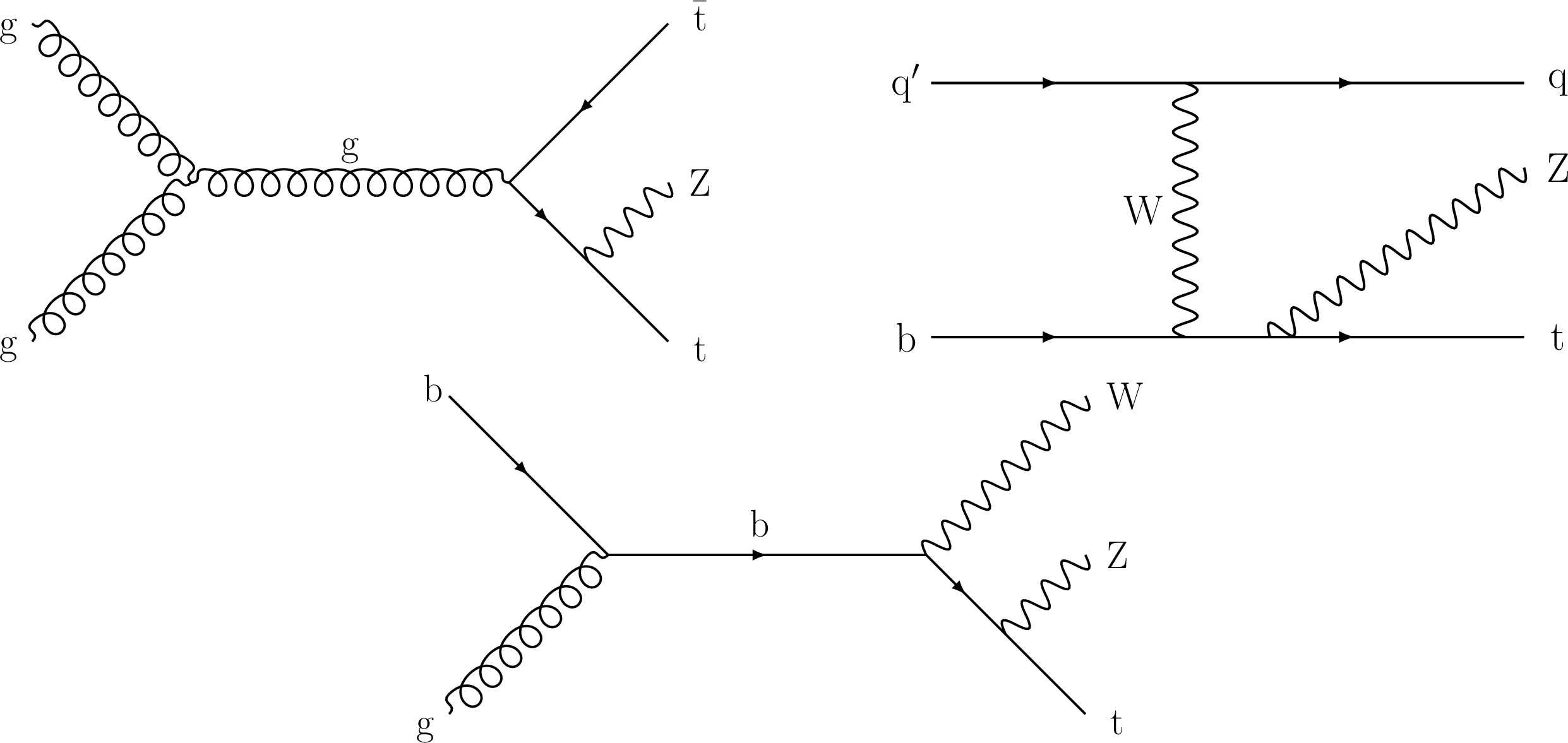
Figure 1:
Representative Feynman diagrams at tree level for ${{\mathrm{t} {}\mathrm{\bar{t}}}}$Z (upper left), tZq (upper right), and tWZ (lower) production. |
png pdf |
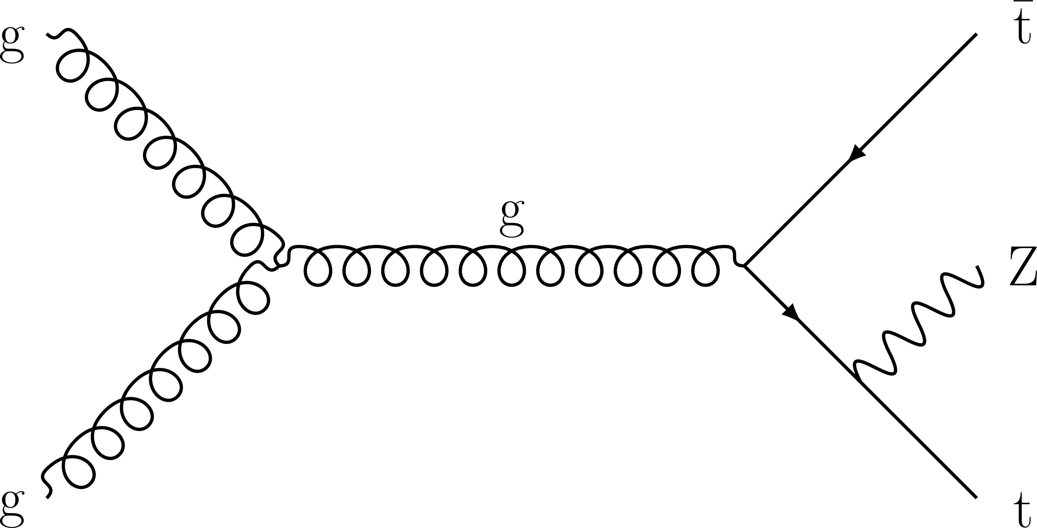
Figure 1-a:
Representative Feynman diagram at tree level for ${{\mathrm{t} {}\mathrm{\bar{t}}}}$Z production. |
png pdf |
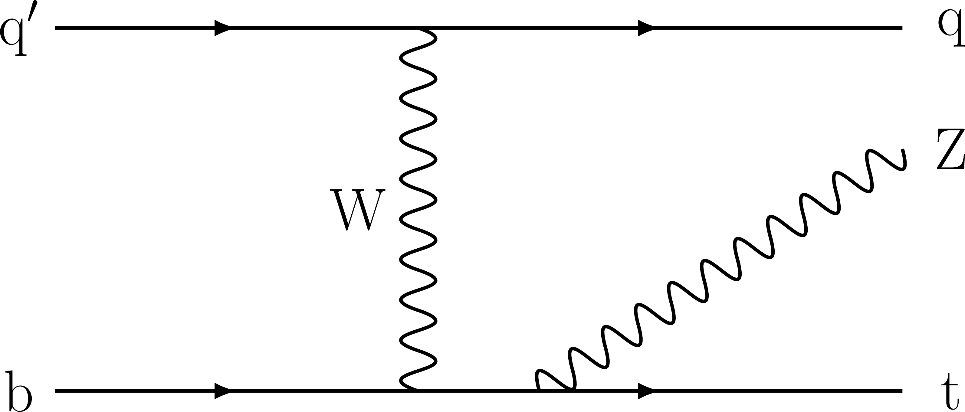
Figure 1-b:
Representative Feynman diagram at tree level for tZq production. |
png pdf |
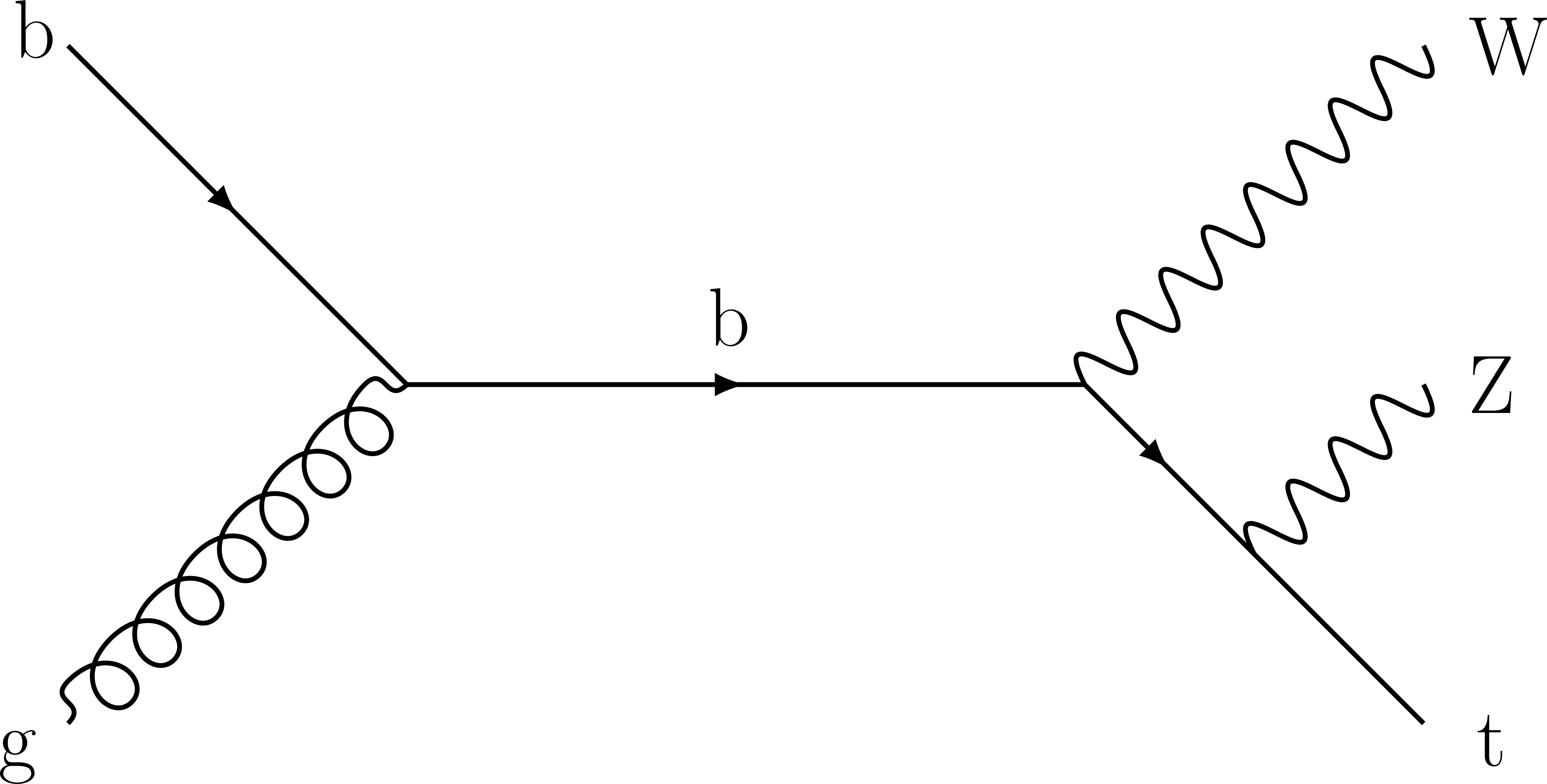
Figure 1-c:
Representative Feynman diagram at tree level for tWZ production. |
png pdf |
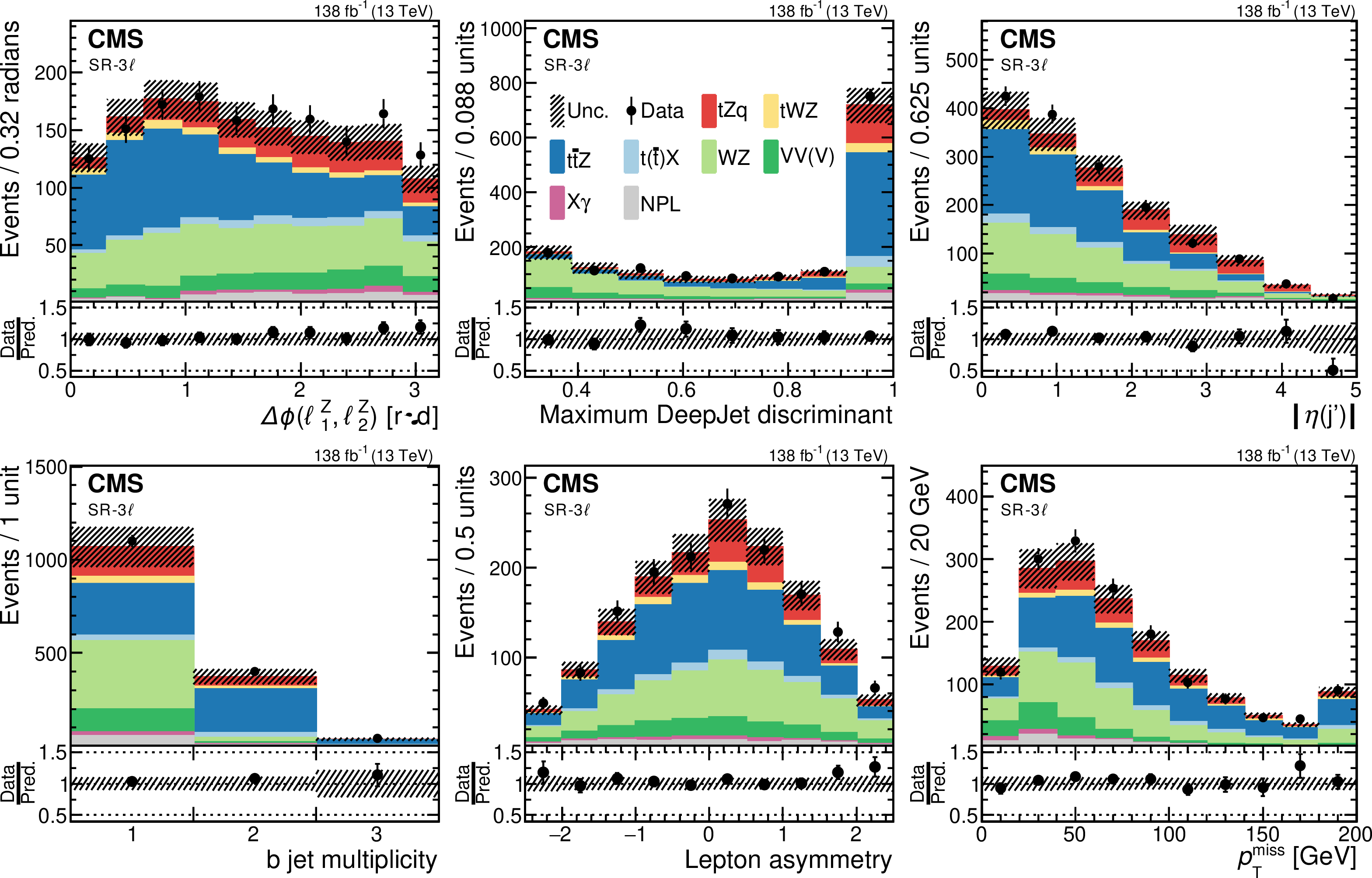
Figure 2:
Pre-fit data-to-simulation comparisons for several observables in the SR-3$\ell$. From left to right and upper to lower, the distributions correspond to: the relative azimuthal angle $\Delta \phi $ between the two leptons from the Z boson decay; the maximum DeepJet discriminant among all selected jets; the absolute pseudorapidity of the recoiling jet; the b jet multiplicity; the lepton asymmetry; and ${{p_{\mathrm {T}}} ^\text {miss}}$. The lower panels display the ratios of the observed event yields to their predicted values. The NPL background is modeled with the procedure based on control samples in data described in Section 6. The hatched band represents the total uncertainty in the prediction. Underflows and overflows are included in the first and last bins, respectively. |

png pdf |
Figure 3:
Pre-fit data-to-simulation comparisons for the distributions of the ${{\mathrm{t} {}\mathrm{\bar{t}}}}$Z (left), tZq (middle), and Others (right) output nodes. For each distribution, only the events that have their maximum value in the corresponding output node are included. The lower panels display the ratios of the observed event yields to their predicted values. The hatched band represents the total uncertainty in the prediction. |

png pdf |
Figure 4:
Post-fit data-to-simulation comparisons for the distributions that are common to all fits, corresponding to counting experiments in the CRs and SR-ttZ-4$\ell$ (left), and to the ${{m_{\mathrm {T}}} ^{\mathrm{W}}}$ observable in the SR-Others (right), after the 5D fit. The lower panels display the ratios of the observed event yields to their post-fit expected values. Overflows are included in the last bin of the right figure. |

png pdf |
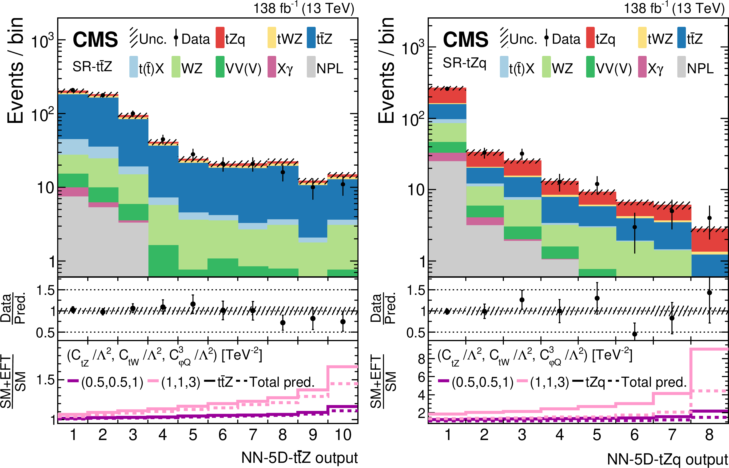
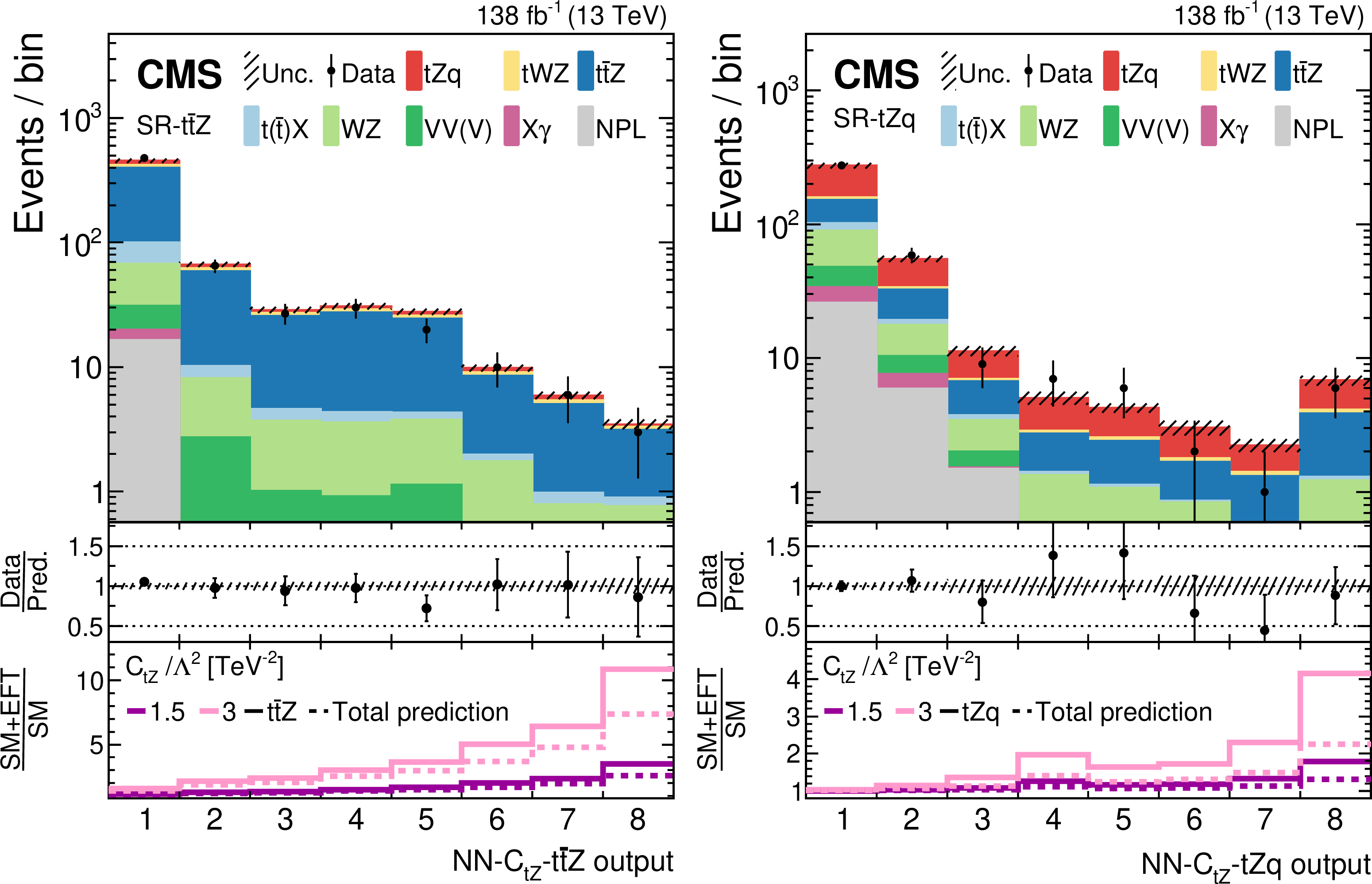
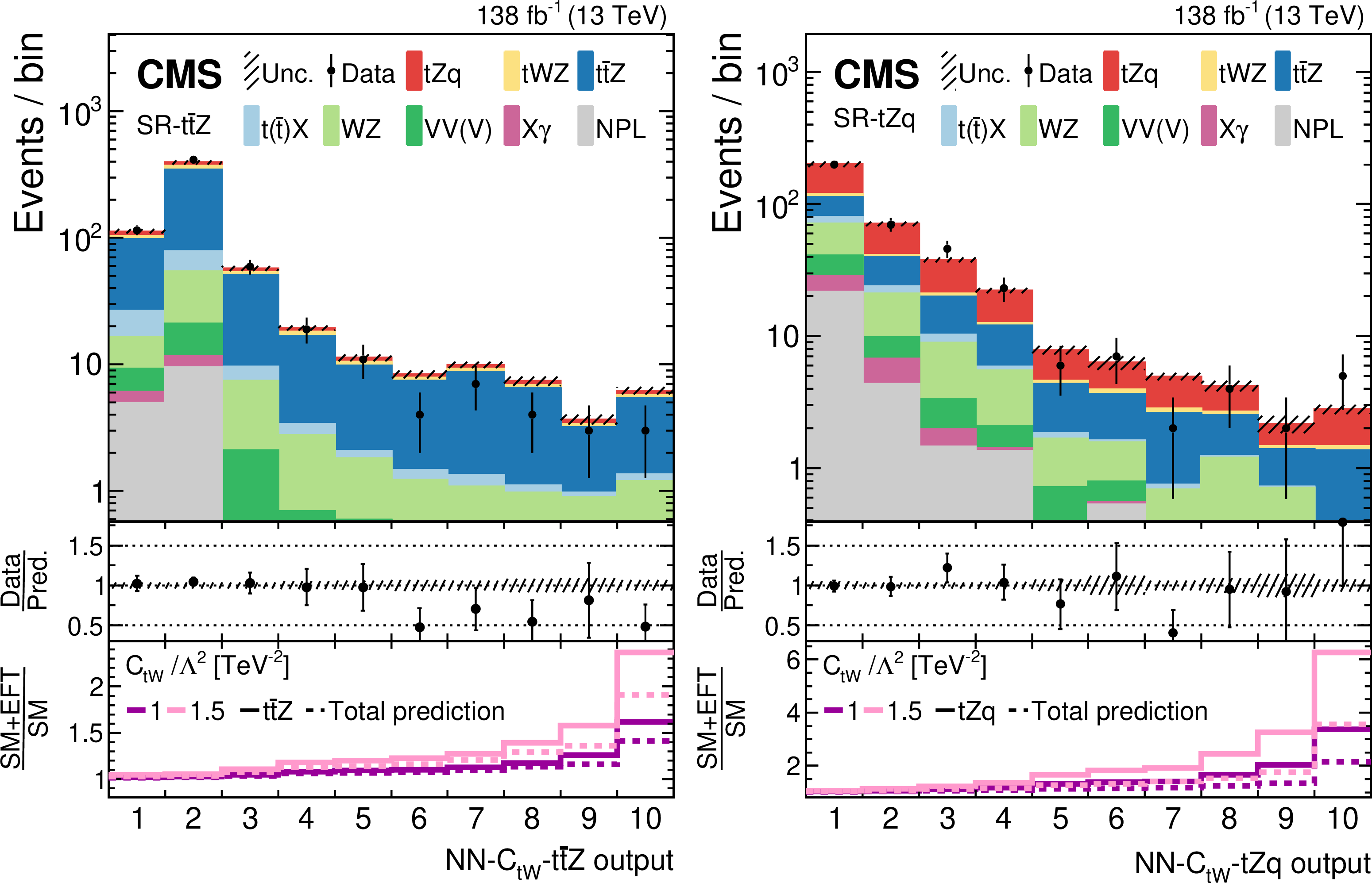
Figure 5:
Post-fit data-to-simulation comparisons for the distributions used in the SR-ttZ (left) and SR-tZq (right), for the 5D fit (upper) and for the 1D fit to ${c_{\mathrm{t} \mathrm{Z}}}$ (lower). The middle panels display the ratios of the observed event yields to their post-fit expected values. For each region, the lower panel shows the change of the event yield in each bin with respect to the SM post-fit expectation for two benchmark EFT scenarios, both for the main signal process in the region (thick lines) and for the total prediction (dashed lines). |
png pdf |
Figure 5-a:
Post-fit data-to-simulation comparisons for the distributions used in the SR-ttZ (left) and SR-tZq (right), for the 5D fit.The middle panels display the ratios of the observed event yields to their post-fit expected values. For each region, the lower panel shows the change of the event yield in each bin with respect to the SM post-fit expectation for two benchmark EFT scenarios, both for the main signal process in the region (thick lines) and for the total prediction (dashed lines). |
png pdf |
Figure 5-b:
Post-fit data-to-simulation comparisons for the distributions used in the SR-ttZ (left) and SR-tZq (right), for the 1D fit to ${c_{\mathrm{t} \mathrm{Z}}}$. The middle panels display the ratios of the observed event yields to their post-fit expected values. For each region, the lower panel shows the change of the event yield in each bin with respect to the SM post-fit expectation for two benchmark EFT scenarios, both for the main signal process in the region (thick lines) and for the total prediction (dashed lines). |
png pdf |
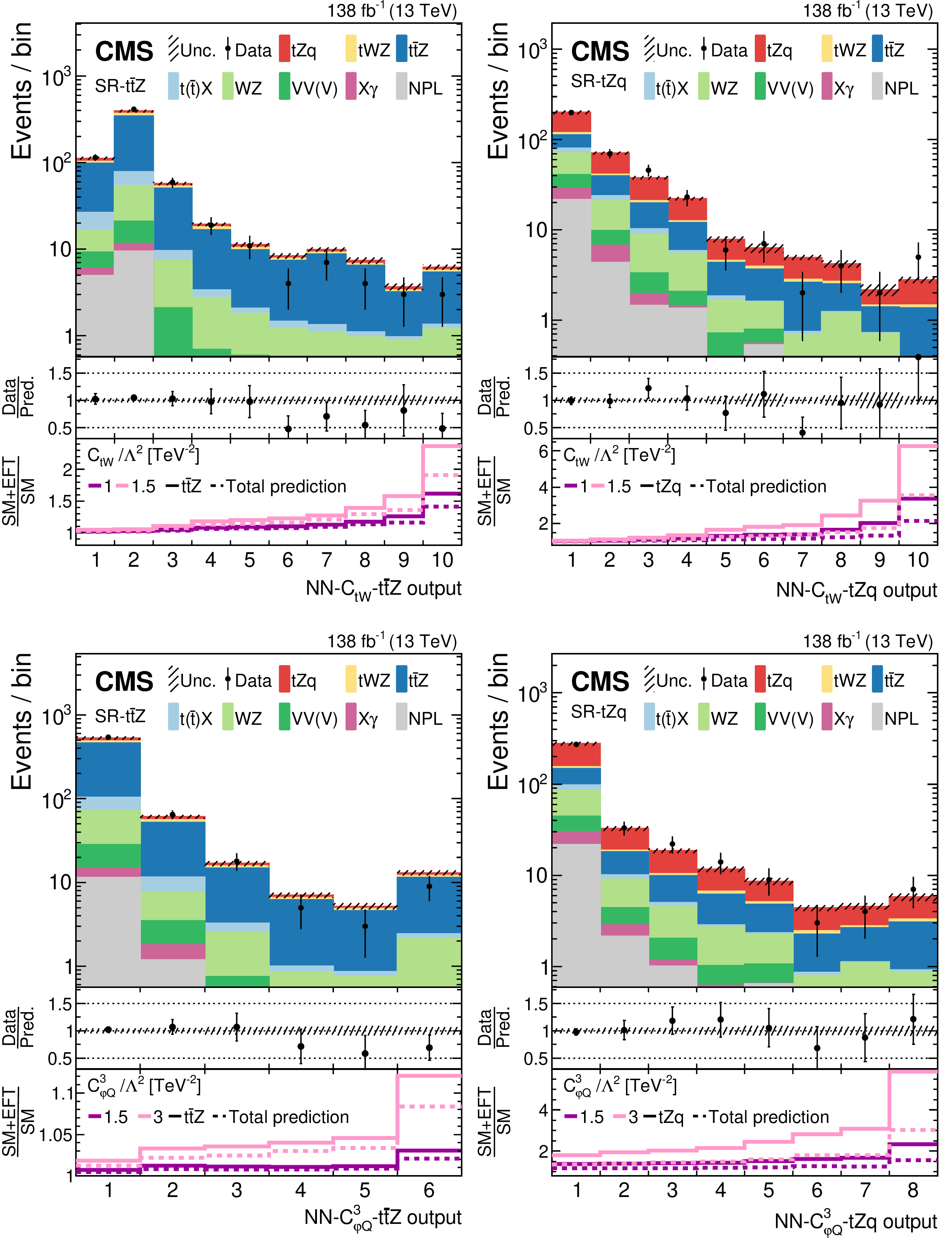
Figure 6:
Post-fit data-to-simulation comparisons for the distributions used in the SR-ttZ (left) and SR-tZq (right), for the 1D fits to ${c_{\mathrm{t} \mathrm{W}}}$ (upper) and to ${c^{3}_{\varphi \mathrm {Q}}}$ (lower). The middle panels display the ratios of the observed event yields to their post-fit expected values. For each region, the lower panel shows the change of the event yield in each bin with respect to the SM prediction for two benchmark EFT scenarios, both for the main signal process in the region (thick lines) and for the total prediction (dashed lines). |
png pdf |
Figure 6-a:
Post-fit data-to-simulation comparisons for the distributions used in the SR-ttZ (left) and SR-tZq (right), for the 1D fits to ${c_{\mathrm{t} \mathrm{W}}}$. The middle panels display the ratios of the observed event yields to their post-fit expected values. For each region, the lower panel shows the change of the event yield in each bin with respect to the SM prediction for two benchmark EFT scenarios, both for the main signal process in the region (thick lines) and for the total prediction (dashed lines). |

png pdf |
Figure 6-b:
Post-fit data-to-simulation comparisons for the distributions used in the SR-ttZ (left) and SR-tZq (right), for the 1D fits to ${c^{3}_{\varphi \mathrm {Q}}}$. The middle panels display the ratios of the observed event yields to their post-fit expected values. For each region, the lower panel shows the change of the event yield in each bin with respect to the SM prediction for two benchmark EFT scenarios, both for the main signal process in the region (thick lines) and for the total prediction (dashed lines). |
png pdf |
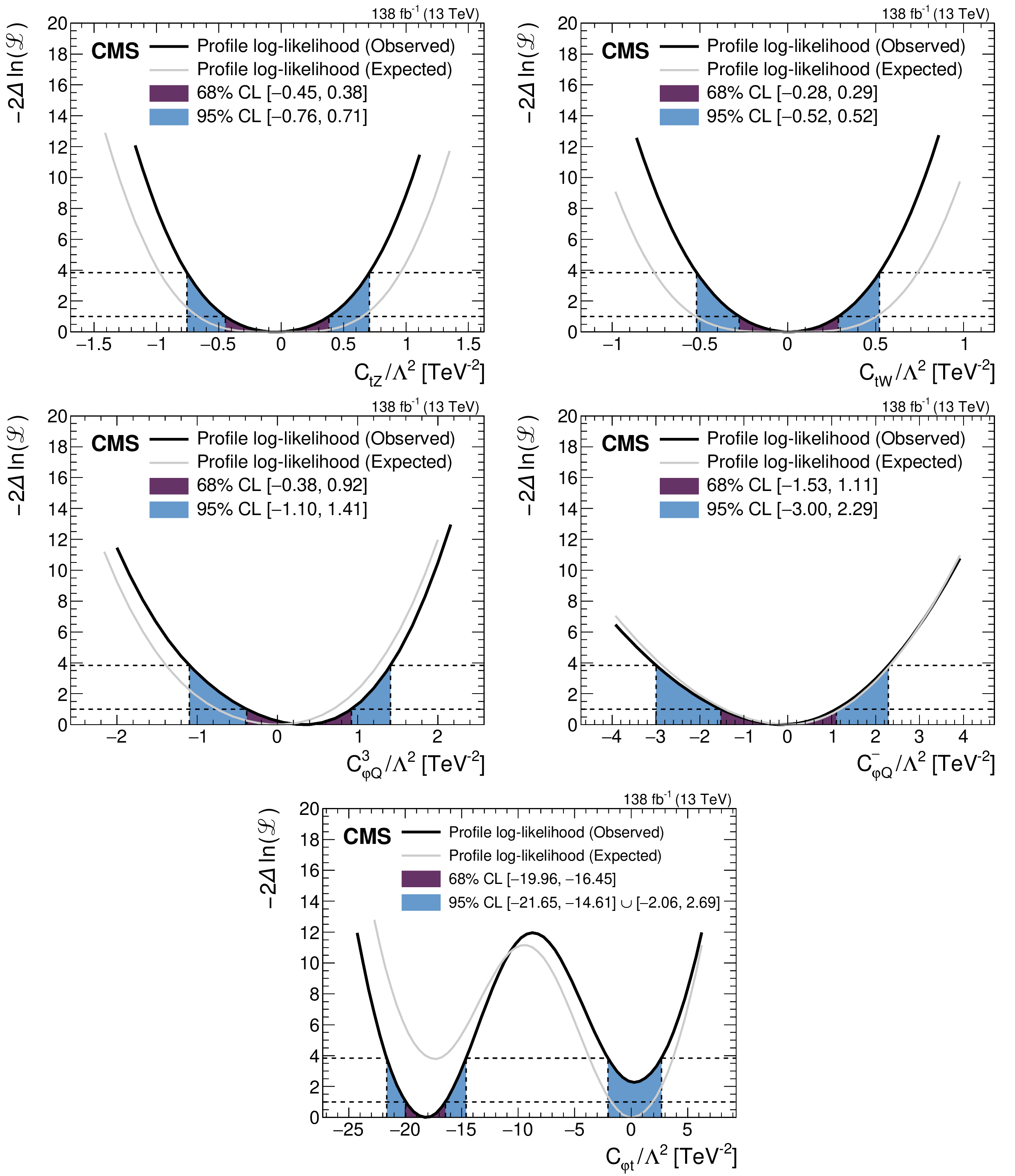
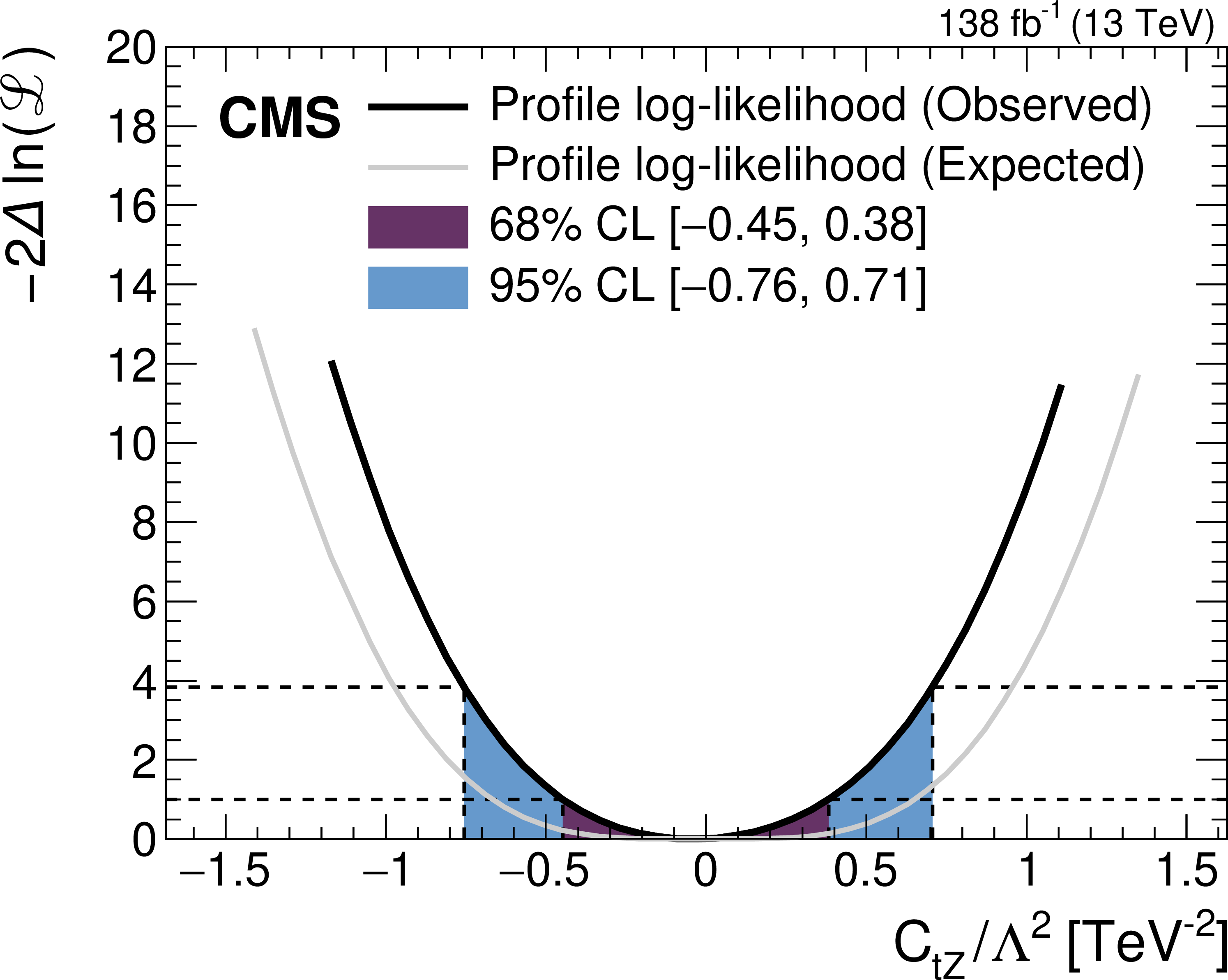
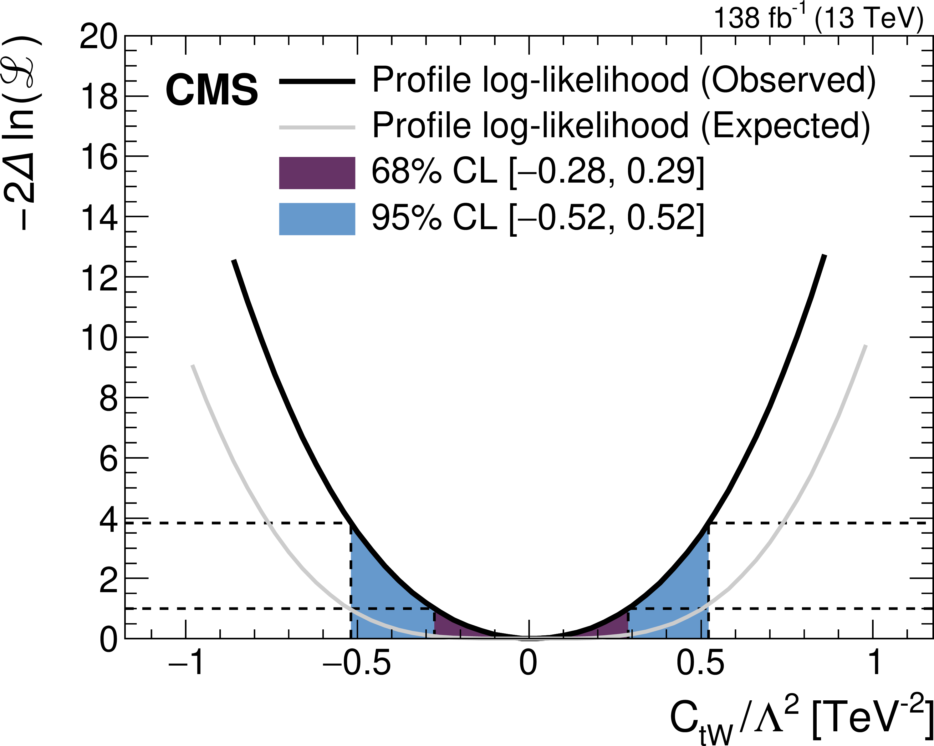
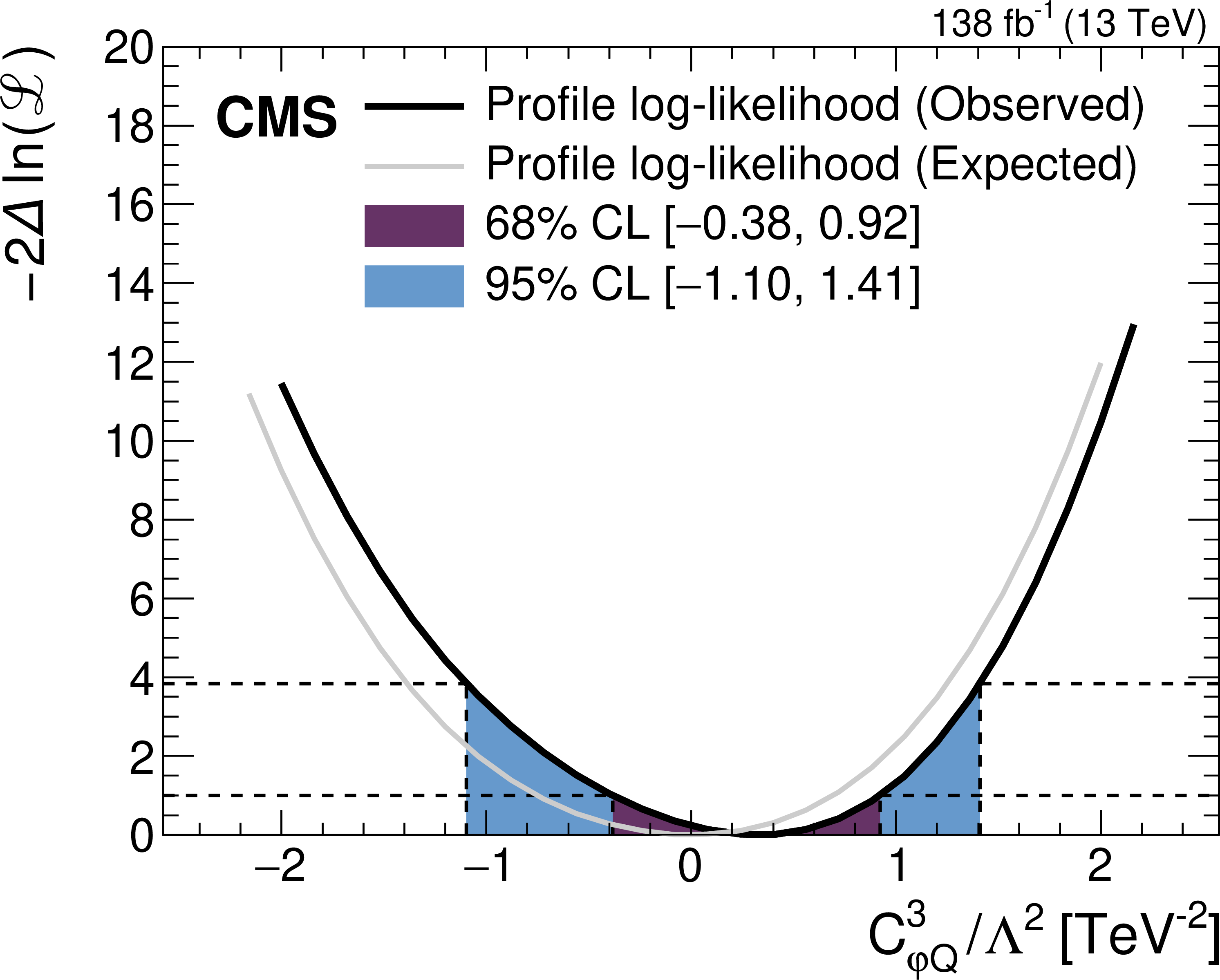
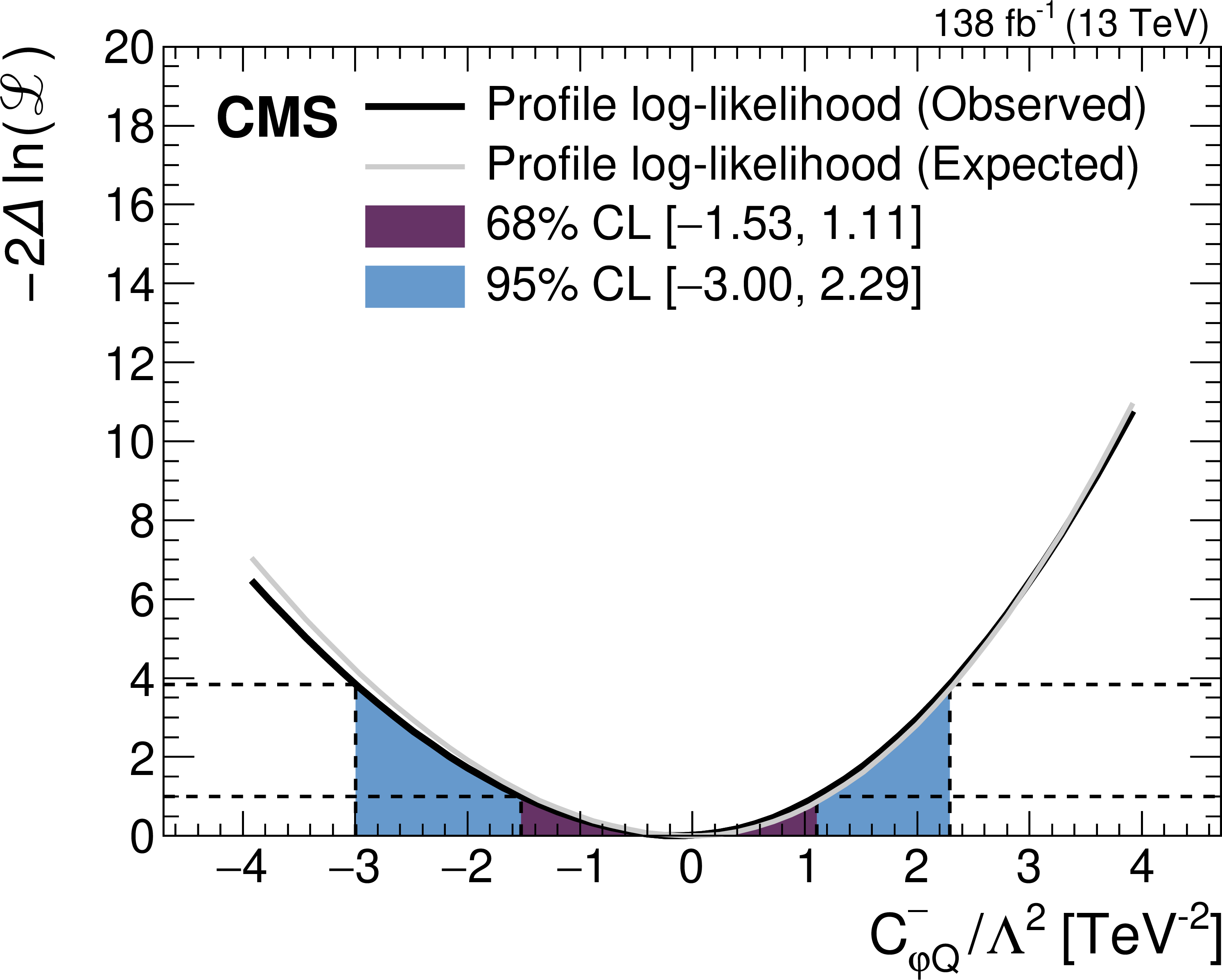
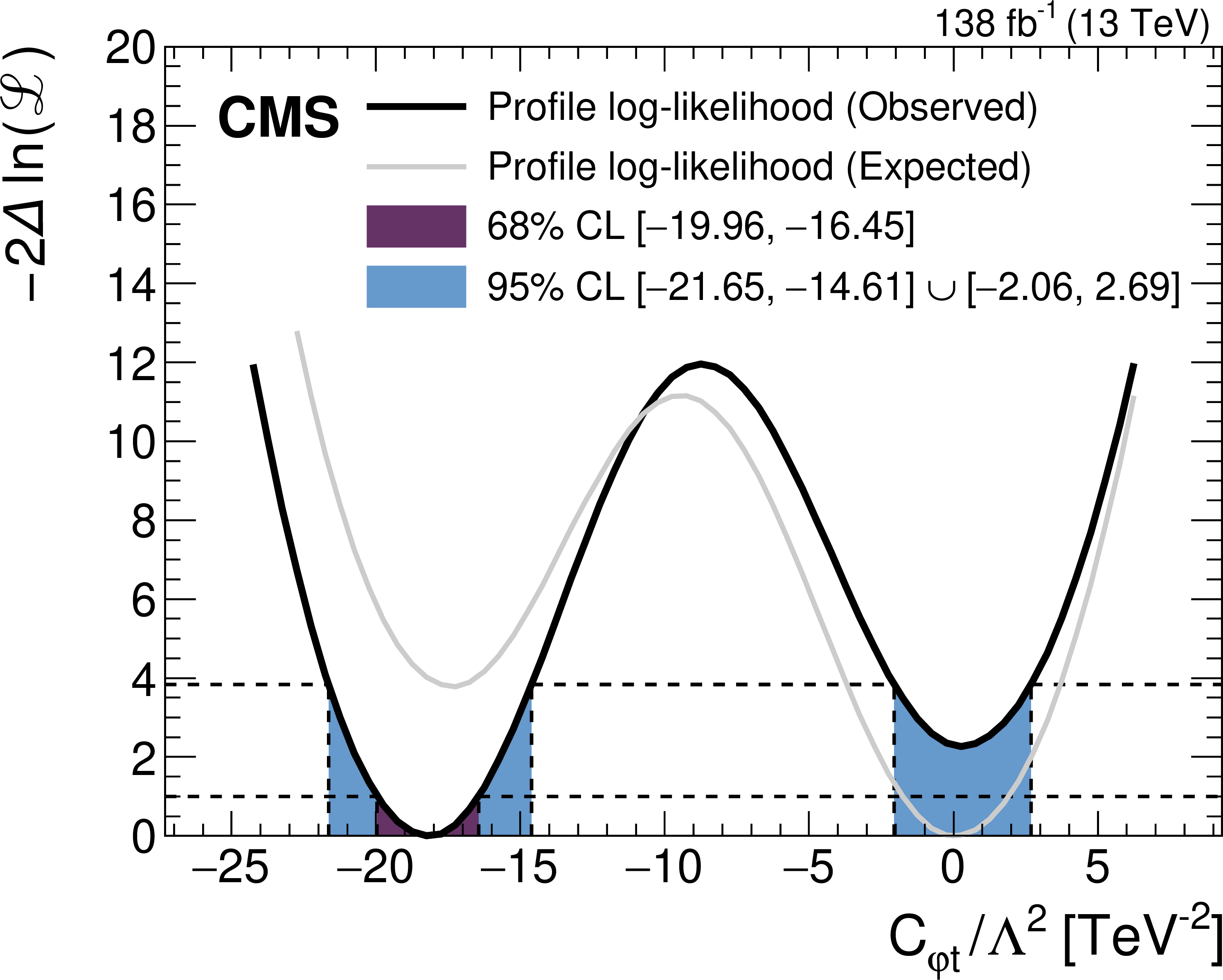
Figure 7:
Observed (thick black lines) and expected (thin gray lines) one-dimensional scans of the negative log-likelihood as a function of each of the five WCs, while fixing the other WCs to their SM values of zero. The 68 and 95% CL confidence intervals are indicated by the colored areas. |
png pdf |
Figure 7-a:
Observed (thick black lines) and expected (thin gray lines) one-dimensional scans of the negative log-likelihood as a function of ${c_{\mathrm{t} \mathrm{Z}}}/\Lambda^2$, while fixing the other WCs to their SM values of zero. The 68 and 95% CL confidence intervals are indicated by the colored areas. |
png pdf |
Figure 7-b:
Observed (thick black lines) and expected (thin gray lines) one-dimensional scans of the negative log-likelihood as a function of ${c_{\mathrm{t} \mathrm{W}}}/\Lambda^2$, while fixing the other WCs to their SM values of zero. The 68 and 95% CL confidence intervals are indicated by the colored areas. |
png pdf |
Figure 7-c:
Observed (thick black lines) and expected (thin gray lines) one-dimensional scans of the negative log-likelihood as a function of ${c^{3}_{\varphi \mathrm {Q}}}/\Lambda^2$, while fixing the other WCs to their SM values of zero. The 68 and 95% CL confidence intervals are indicated by the colored areas. |
png pdf |
Figure 7-d:
Observed (thick black lines) and expected (thin gray lines) one-dimensional scans of the negative log-likelihood as a function of ${c^{-}_{\varphi \mathrm {Q}}}/\Lambda^2$, while fixing the other WCs to their SM values of zero. The 68 and 95% CL confidence intervals are indicated by the colored areas. |
png pdf |
Figure 7-e:
Observed (thick black lines) and expected (thin gray lines) one-dimensional scans of the negative log-likelihood as a function of ${c_{\varphi \mathrm{t}}}/\Lambda^2$, while fixing the other WCs to their SM values of zero. The 68 and 95% CL confidence intervals are indicated by the colored areas. |

png pdf |
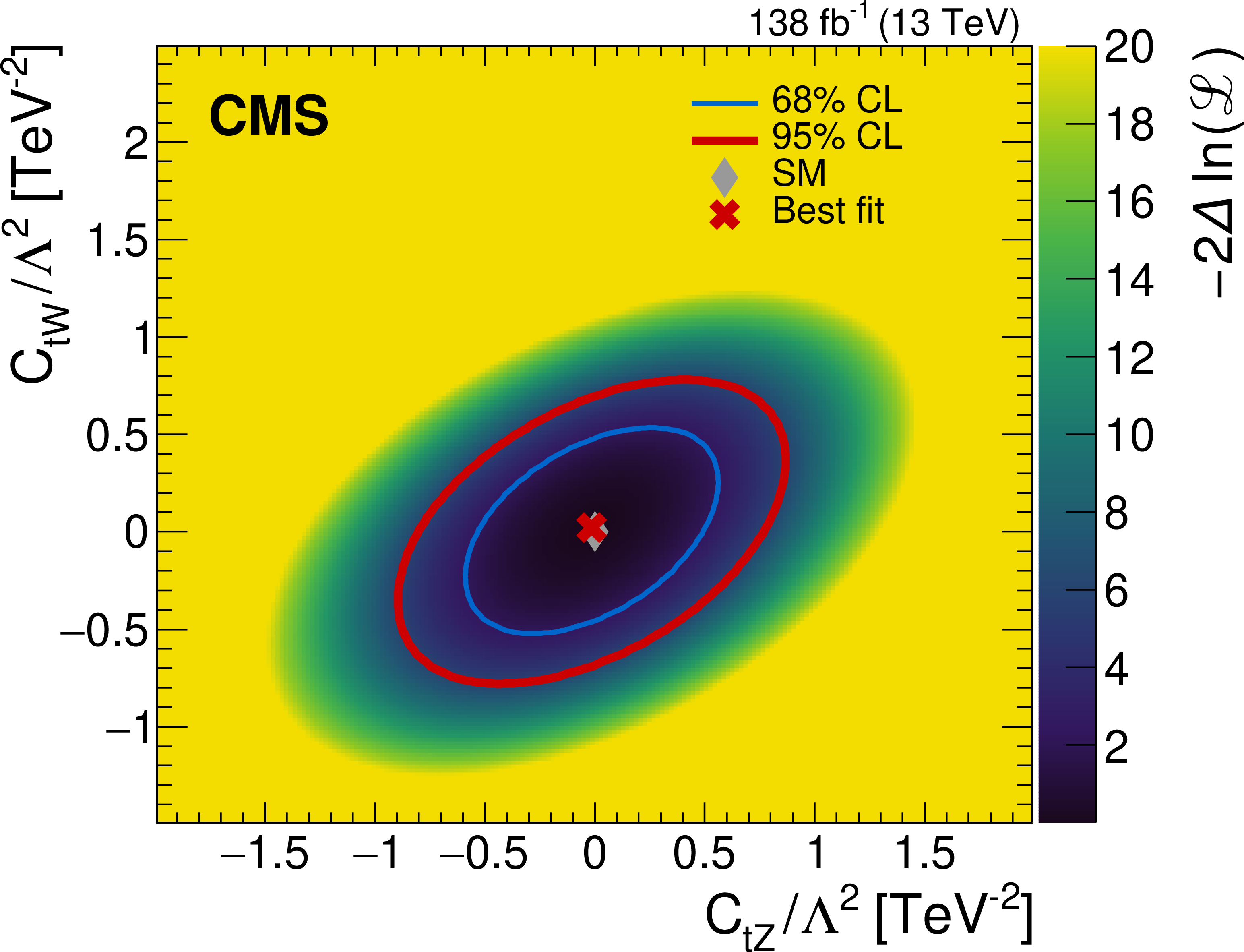
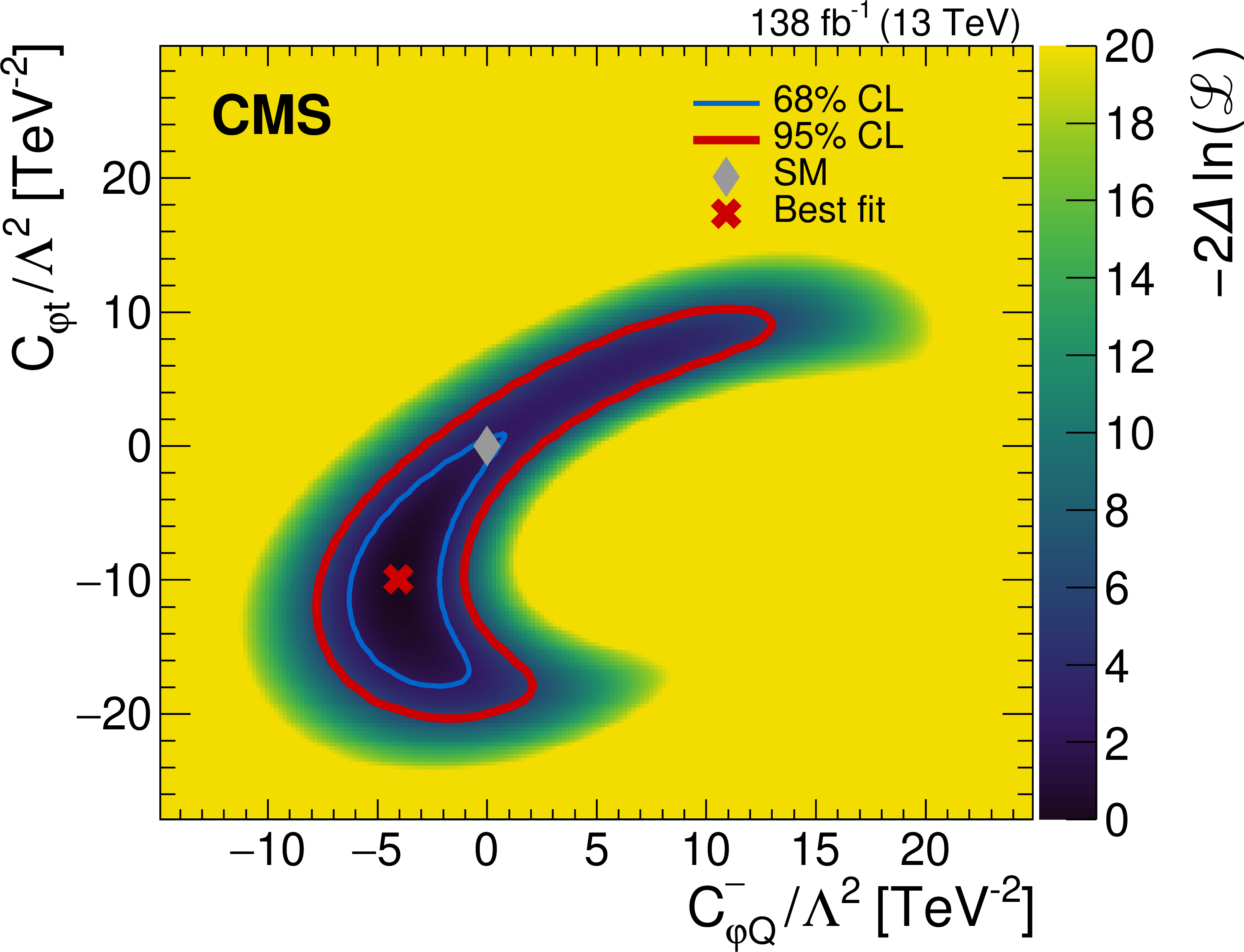
Figure 8:
Two-dimensional scans of the negative log-likelihood as a function of ${c_{\mathrm{t} \mathrm{Z}}}$ and ${c_{\mathrm{t} \mathrm{W}}}$ (left), or as a function of ${c^{-}_{\varphi \mathrm {Q}}}$ and ${c_{\varphi \mathrm{t}}}$ (right), while fixing the other WCs to their SM values of zero. The SM and best fit points are indicated by diamond- and cross-shaped markers, respectively. The thin blue line and thick red line represent the 68 and 95% CL contours, respectively. |
png pdf |
Figure 8-a:
Two-dimensional scans of the negative log-likelihood as a function of ${c_{\mathrm{t} \mathrm{Z}}}$ and ${c_{\mathrm{t} \mathrm{W}}}$, while fixing the other WCs to their SM values of zero. The SM and best fit points are indicated by diamond- and cross-shaped markers, respectively. The thin blue line and thick red line represent the 68 and 95% CL contours, respectively. |
png pdf |
Figure 8-b:
Two-dimensional scans of the negative log-likelihood as a function of ${c^{-}_{\varphi \mathrm {Q}}}$ and ${c_{\varphi \mathrm{t}}}$, while fixing the other WCs to their SM values of zero. The SM and best fit points are indicated by diamond- and cross-shaped markers, respectively. The thin blue line and thick red line represent the 68 and 95% CL contours, respectively. |
| Tables | |
png pdf |
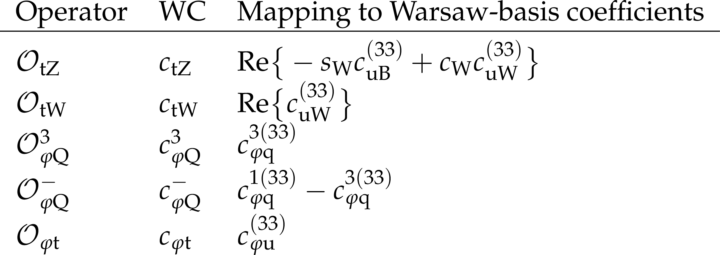
Table 1:
List of dimension-six EFT operators considered in this analysis and their corresponding WCs. The linear combinations of WCs to which they correspond in the Warsaw basis are indicated. The abbreviations $ {s_{\mathrm {W}}} $ and $ {c_{\mathrm {W}}} $ denote the sine and cosine of the weak mixing angle, respectively. The definitions of the relevant Warsaw-basis operators can be found in Ref. [19]. |
png pdf |
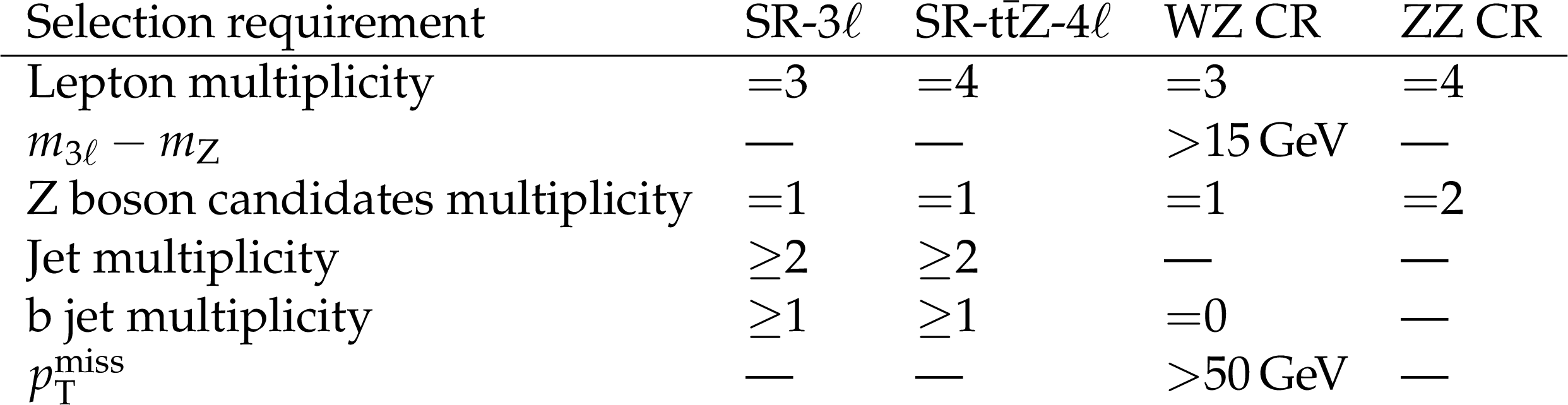
Table 2:
Summary of the main selection requirements applied in each signal or control region. A dash indicates that the selection requirement is not applied. |

png pdf |
Table 3:
Input variables to the NN-SM and to the eight {NN-EFTs}. A dash indicates that the variable is not used. The three-momentum of an object includes the ${p_{\mathrm {T}}}$, $\eta $, and $\phi $ components of its momentum. The symbol $\ell _{\mathrm{t}}$ denotes the lepton produced in the decay of the top quark; $j'$ denotes the recoiling jet; $b$ denotes the b jet associated with the leptonic top quark decay; $(\ell ^{\mathrm{Z}}_{1},\ell ^{\mathrm{Z}}_{2})$ denote the leptons produced in the Z boson decay; ${\cos\theta ^{\star}_{\mathrm{Z}}}$ is the cosine of the angle between the direction of the Z boson in the detector reference frame, and the direction of the negatively-charged lepton from the Z boson decay in the rest frame of the Z boson. Other observables are defined in Section 4. |
png pdf |
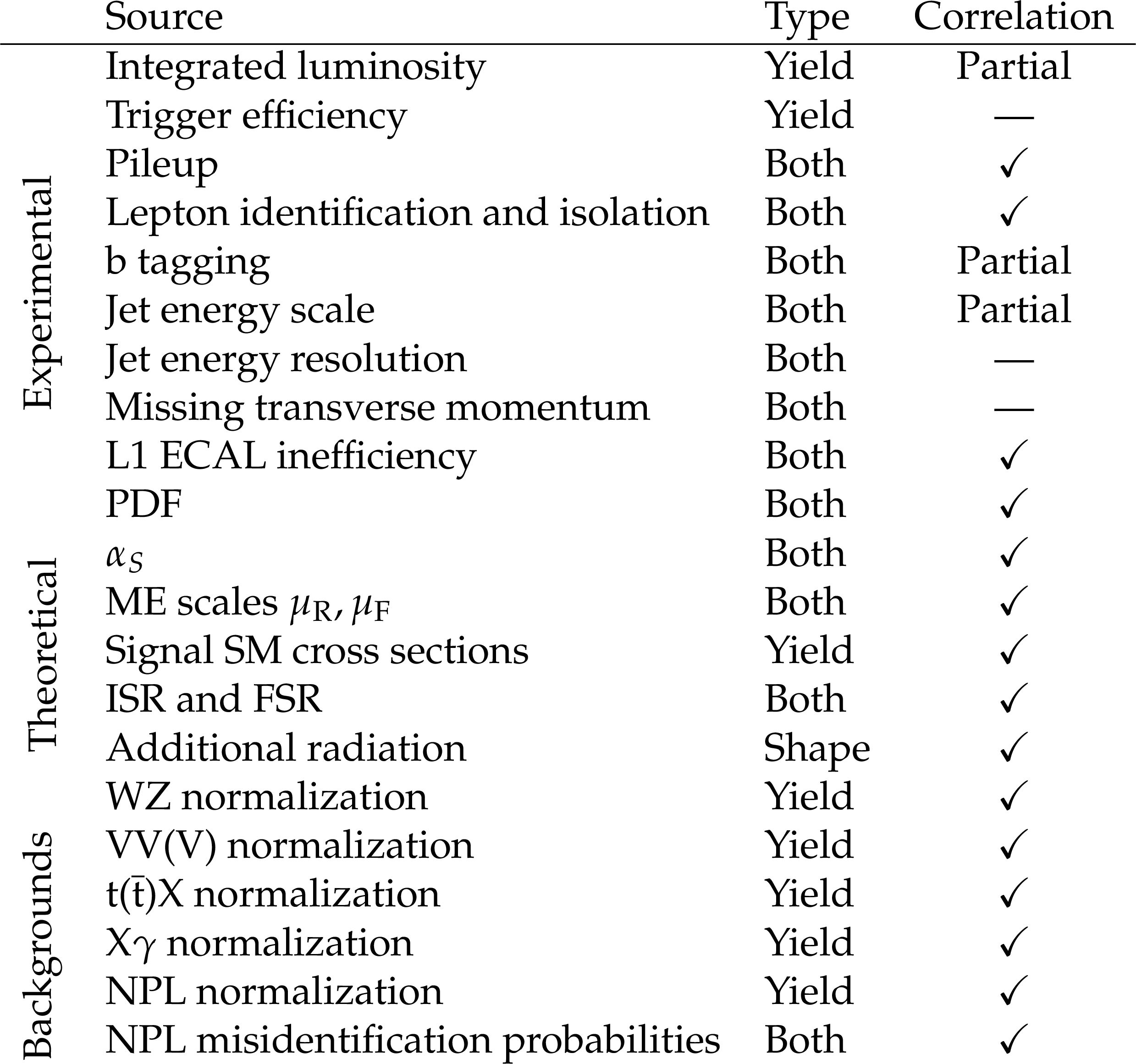
Table 4:
Summary of the different sources of systematic uncertainty included in the measurements. The first column indicates the source of the uncertainty. The second column indicates whether the source affects the event yields, the shapes of the observables, or both. In the third column, the symbols "v'' and "--'' indicate 100% and 0% correlations between the data-taking periods, respectively. |

png pdf |
Table 5:
Observables used in each region for the different fits. The NN-SM is trained to separate different SM processes, while the other NNs are trained to identify new effects arising from one or more EFT operators, as described in Section 7. |

png pdf |
Table 6:
Expected and observed 95% CL confidence intervals for all WCs. The intervals in the first and second columns are obtained by scanning over a single WC, while fixing the other WCs to their SM values of zero. The intervals in the third and fourth columns are obtained by performing a 5D fit in which all five WCs are treated as free parameters. As explained in Section 9, the 1D intervals are obtained from separate fits to different observables in the SR-tZq and SR-ttZ, while the 5D intervals are obtained from a single fit. |

png pdf |
Table 7:
Impacts from different groups of sources of systematic uncertainty on each individual WC. To estimate the impact of a given group, the corresponding sources of systematic uncertainty are excluded, the 1D fits to the data are repeated, and the reduction in the width of the confidence interval is quoted for each WC. The values are given in percent. |
| Summary |
|
A search for new top quark interactions has been performed within the framework of an effective field theory (EFT) using the associated production of either one or two top quarks with a Z boson in multilepton final states. The data sample corresponds to an integrated luminosity of 138 fb$^{-1}$ of proton-proton collisions at $\sqrt{s} = $ 13 TeV collected by the CMS experiment. Five dimension-six operators modifying the electroweak interactions of the top quark were considered. The event yields and kinematic properties of the signal processes were parameterized with Wilson coefficients (WCs) describing the interaction strengths of these operators. A multivariate analysis relying upon machine-learning techniques was designed to enhance the sensitivity to effects arising from the EFT operators. A multiclass neural network was trained to distinguish between standard model (SM) processes and was used to define three subregions enriched in tZq, ttZ, and background events. Additional neural networks were trained to separate events generated according to the SM from events generated with nonzero WC values, and were used to construct optimal observables. This is the first time that machine-learning techniques accounting for the interference between EFT operators and the SM amplitude have been used in an LHC analysis. Results were extracted from a simultaneous fit to data in six event categories. Two confidence intervals were determined for each WC, one keeping the other WCs fixed to zero and the other treating all five WCs as free parameters. Two-dimensional contours were produced for pairs of WCs to illustrate their correlations. All results are consistent with the SM at 95% confidence level. |
| References | ||||
| 1 | Particle Data Group, P. A. Zyla et al. | Review of particle physics | Prog. Theor. Exp. Phys. 2020 (2020) 083C01 | |
| 2 | L. Canetti, M. Drewes, and M. Shaposhnikov | Matter and antimatter in the universe | New J. Phys. 14 (2012) 095012 | 1204.4186 |
| 3 | K. Arun, S. B. Gudennavar, and C. Sivaram | Dark matter, dark energy, and alternate models: A review | Adv. Space Res. 60 (2017) 166 | 1704.06155 |
| 4 | W. Buchmuller and D. Wyler | Effective lagrangian analysis of new interactions and flavour conservation | NPB 268 (1986) 621 | |
| 5 | C. P. Burgess | Introduction to effective field theory | Ann. Rev. Nucl. Part. Sci. 57 (2007) 329 | hep-th/0701053 |
| 6 | A. Helset and A. Kobach | Baryon number, lepton number, and operator dimension in the SMEFT with flavor symmetries | PLB 800 (2020) 135132 | 1909.05853 |
| 7 | CMS Collaboration | Measurement of the top quark mass using proton-proton data at $ \sqrt{s}= $ 7 and 8 TeV | PRD 93 (2016) 072004 | CMS-TOP-14-022 1509.04044 |
| 8 | B. A. Dobrescu and C. T. Hill | Electroweak symmetry breaking via top condensation seesaw | PRL 81 (1998) 2634 | hep-ph/9712319 |
| 9 | R. S. Chivukula, B. A. Dobrescu, H. Georgi, and C. T. Hill | Top quark seesaw theory of electroweak symmetry breaking | PRD 59 (1999) 075003 | hep-ph/9809470 |
| 10 | D. Delepine, J. M. Gerard, and R. Gonzalez Felipe | Is the standard Higgs scalar elementary? | PLB 372 (1996) 271 | hep-ph/9512339 |
| 11 | CMS Collaboration | Observation of single top quark production in association with a $ \mathrm{Z} $ boson in proton-proton collisions at $ \sqrt {s} = $ 13 TeV | PRL 122 (2019) 132003 | CMS-TOP-18-008 1812.05900 |
| 12 | ATLAS Collaboration | Observation of the associated production of a top quark and a $ \mathrm{Z} $ boson in $ {\mathrm{p}}{\mathrm{p}} $ collisions at $ \sqrt{s} = $ 13 TeV with the ATLAS detector | JHEP 07 (2020) 124 | 2002.07546 |
| 13 | CMS Collaboration | Observation of top quark pairs produced in association with a vector boson in pp collisions at $ \sqrt{s}= $ 8 TeV | JHEP 01 (2016) 096 | CMS-TOP-14-021 1510.01131 |
| 14 | ATLAS Collaboration | Measurements of the inclusive and differential production cross sections of a top-quark-antiquark pair in association with a $ \mathrm{Z} $ boson at $ \sqrt{s} = $ 13 TeV with the ATLAS detector | Submitted to EPJC | 2103.12603 |
| 15 | C. Grojean, O. Matsedonskyi, and G. Panico | Light top partners and precision physics | JHEP 10 (2013) 160 | 1306.4655 |
| 16 | T. Ibrahim and P. Nath | The chromoelectric dipole moment of the top quark in models with vector like multiplets | PRD 84 (2011) 015003 | 1104.3851 |
| 17 | R. S. Chivukula, E. H. Simmons, and J. Terning | A heavy top quark and the $ \mathrm{Z}\mathrm{b\bar{b}} $ vertex in non-commuting extended technicolor | PLB 331 (1994) 383 | hep-ph/9404209 |
| 18 | CMS Collaboration | Measurement of the top quark polarization and $ \mathrm{t\bar{t}} $ spin correlations using dilepton final states in proton-proton collisions at $ \sqrt{s} = $ 13 TeV | PRD 100 (2019) 072002 | CMS-TOP-18-006 1907.03729 |
| 19 | J. A. Aguilar-Saavedra et al. | Interpreting top-quark LHC measurements in the standard-model effective field theory | 1802.07237 | |
| 20 | I. Brivio et al. | O new physics, where art thou? A global search in the top sector | JHEP 02 (2020) 131 | 1910.03606 |
| 21 | F. Maltoni, L. Mantani, and K. Mimasu | Top-quark electroweak interactions at high energy | JHEP 10 (2019) 004 | 1904.05637 |
| 22 | J. Brehmer, K. Cranmer, G. Louppe, and J. Pavez | A guide to constraining effective field theories with machine learning | PRD 98 (2018) 052004 | 1805.00020 |
| 23 | J. Hollingsworth and D. Whiteson | Resonance searches with machine learned likelihood ratios | Submitted to SciPost Physics | 2002.04699 |
| 24 | F. F. Freitas, C. K. Khosa, and V. Sanz | Exploring the standard model EFT in $ \mathrm{\mathrm{V}\mathrm{H}} $ production with machine learning | PRD 100 (2019) 035040 | 1902.05803 |
| 25 | CMS Collaboration | Search for new physics in top quark production with additional leptons in proton-proton collisions at $ \sqrt{s} = $ 13 TeV using effective field theory | JHEP 03 (2021) 095 | CMS-TOP-19-001 2012.04120 |
| 26 | CMS Collaboration | Precision luminosity measurement in proton-proton collisions at $ \sqrt{s}= $ 13 TeV in 2015 and 2016 at CMS | Submitted to EPJC | CMS-LUM-17-003 2104.01927 |
| 27 | CMS Collaboration | CMS luminosity measurement for the 2017 data-taking period at $ \sqrt{s} = $ 13 TeV | ||
| 28 | CMS Collaboration | CMS luminosity measurement for the 2018 data-taking period at $ \sqrt{s} = $ 13 TeV | ||
| 29 | CMS Collaboration | HEPData record for this analysis | link | |
| 30 | CMS Collaboration | Performance of the CMS Level-1 trigger in proton-proton collisions at $ \sqrt{s} = $ 13 TeV | JINST 15 (2020) P10017 | CMS-TRG-17-001 2006.10165 |
| 31 | CMS Collaboration | The CMS trigger system | JINST 12 (2017) P01020 | CMS-TRG-12-001 1609.02366 |
| 32 | CMS Collaboration | The CMS experiment at the CERN LHC | JINST 3 (2008) S08004 | CMS-00-001 |
| 33 | J. Alwall et al. | The automated computation of tree-level and next-to-leading order differential cross sections, and their matching to parton shower simulations | JHEP 07 (2014) 079 | 1405.0301 |
| 34 | J. M. Campbell, R. K. Ellis, and C. Williams | Vector boson pair production at the LHC | JHEP 07 (2011) 018 | |
| 35 | J. M. Campbell and R. K. Ellis | Update on vector boson pair production at hadron colliders | PRD 60 (1999) 113006 | hep-ph/9905386 |
| 36 | P. Nason | A new method for combining NLO QCD with shower Monte Carlo algorithms | JHEP 11 (2004) 040 | hep-ph/0409146 |
| 37 | S. Frixione, P. Nason, and C. Oleari | Matching NLO QCD computations with parton shower simulations: the $ POWHEG $ method | JHEP 11 (2007) 070 | 0709.2092 |
| 38 | S. Alioli, P. Nason, C. Oleari, and E. Re | A general framework for implementing NLO calculations in shower Monte Carlo programs: the $ POWHEG \textscbox $ | JHEP 06 (2010) 043 | 1002.2581 |
| 39 | P. Nason and G. Zanderighi | $ \mathrm{W^{+}} \mathrm{W^{-}} $, $ \mathrm{W} \mathrm{Z} $ and $ \mathrm{Z} \mathrm{Z} $ production in the POWHEG-BOX-V2 | EPJC 74 (2014) 2702 | 1311.1365 |
| 40 | H. B. Hartanto, B. Jager, L. Reina, and D. Wackeroth | Higgs boson production in association with top quarks in the POWHEG BOX | PRD 91 (2015) 094003 | 1501.04498 |
| 41 | F. Maltoni, G. Ridolfi, and M. Ubiali | $ \mathrm{b} $-initiated processes at the LHC: a reappraisal | JHEP 07 (2012) 022 | 1203.6393 |
| 42 | NNPDF Collaboration | Parton distributions from high-precision collider data | EPJC 77 (2017) 663 | 1706.00428 |
| 43 | NNPDF Collaboration | Parton distributions for the LHC Run 2 | JHEP 04 (2015) 040 | 1410.8849 |
| 44 | T. Sjostrand et al. | An introduction to PYTHIA 8.2 | CPC 191 (2015) 159 | 1410.3012 |
| 45 | CMS Collaboration | Extraction and validation of a new set of CMS $ PYTHIA 8 $ tunes from underlying-event measurements | EPJC 80 (2020) 4 | CMS-GEN-17-001 1903.12179 |
| 46 | CMS Collaboration | Investigations of the impact of the parton shower tuning in $ PYTHIA 8 $ in the modelling of $ \mathrm{t\overline{t}} $ at $ \sqrt{s}= $ 8 and 13 TeV | CMS-PAS-TOP-16-021 | CMS-PAS-TOP-16-021 |
| 47 | CMS Collaboration | Event generator tunes obtained from underlying event and multiparton scattering measurements | EPJC 76 (2016) 155 | CMS-GEN-14-001 1512.00815 |
| 48 | R. Frederix and S. Frixione | Merging meets matching in MC@NLO | JHEP 12 (2012) 061 | 1209.6215 |
| 49 | Alwall, J. et al. | Comparative study of various algorithms for the merging of parton showers and matrix elements in hadronic collisions | EPJC 53 (2008) 473 | 0706.2569 |
| 50 | GEANT4 Collaboration | GEANT4--a simulation toolkit | NIMA 506 (2003) 250 | |
| 51 | P. Artoisenet, R. Frederix, O. Mattelaer, and R. Rietkerk | Automatic spin-entangled decays of heavy resonances in Monte Carlo simulations | JHEP 03 (2013) 015 | 1212.3460 |
| 52 | B. Grzadkowski, M. Iskrzynski, M. Misiak, and J. Rosiek | Dimension-six terms in the standard model Lagrangian | JHEP 10 (2010) 085 | 1008.4884 |
| 53 | LHC Higgs Cross Section Working Group | Handbook of LHC Higgs cross sections: 4. deciphering the nature of the Higgs sector | CERN (2016) | 1610.07922 |
| 54 | CMS Collaboration | Measurement of the associated production of a single top quark and a $ \mathrm{Z} $ boson in $ {\mathrm{p}}{\mathrm{p}} $ collisions at $ \sqrt{s}= $ 13 TeV | PLB 779 (2018) 358 | CMS-TOP-16-020 1712.02825 |
| 55 | CMS Collaboration | Particle-flow reconstruction and global event description with the CMS detector | JINST 12 (2017) P10003 | CMS-PRF-14-001 1706.04965 |
| 56 | M. Cacciari, G. P. Salam, and G. Soyez | The anti-$ {k_{\mathrm{T}}} $ jet clustering algorithm | JHEP 04 (2008) 063 | 0802.1189 |
| 57 | M. Cacciari, G. P. Salam, and G. Soyez | FastJet user manual | EPJC 72 (2012) 1896 | 1111.6097 |
| 58 | CMS Collaboration | Performance of electron reconstruction and selection with the CMS detector in proton-proton collisions at $ \sqrt{s} = $ 8 TeV | JINST 10 (2015) P06005 | CMS-EGM-13-001 1502.02701 |
| 59 | CMS Collaboration | Performance of the CMS muon detector and muon reconstruction with proton-proton collisions at $ \sqrt{s} = $ 13 TeV | JINST 13 (2018) P06015 | CMS-MUO-16-001 1804.04528 |
| 60 | CMS Collaboration | Measurement of the Higgs boson production rate in association with top quarks in final states with electrons, muons, and hadronically decaying tau leptons at $ \sqrt{s} = $ 13 TeV | EPJC 81 (2021) 378 | CMS-HIG-19-008 2011.03652 |
| 61 | M. Cacciari and G. P. Salam | Pileup subtraction using jet areas | PLB 659 (2008) 119 | 0707.1378 |
| 62 | CMS Collaboration | Jet energy scale and resolution in the CMS experiment in pp collisions at 8 TeV | JINST 12 (2017) P02014 | CMS-JME-13-004 1607.03663 |
| 63 | CMS Collaboration | Identification of heavy-flavour jets with the CMS detector in pp collisions at 13 TeV | JINST 13 (2018) P05011 | CMS-BTV-16-002 1712.07158 |
| 64 | E. Bols et al. | Jet flavour classification using $ \DeepJet $ | JINST 15 (2020) P12012 | 2008.10519 |
| 65 | B. R. Vormwald | The CMS Phase-1 pixel detector---experience and lessons learned from two years of operation | JINST 14 (2019) C07008 | |
| 66 | CMS Collaboration | Performance of the $ \DeepJet \Pqb\ $ tagging algorithm using 41.9 fb$ ^{-1} $ of data from proton-proton collisions at 13 TeV with Phase-1 CMS detector | CDS | |
| 67 | CMS Collaboration | Performance of missing transverse momentum reconstruction in proton-proton collisions at $ \sqrt{s} = $ 13 TeV using the CMS detector | JINST 14 (2019) P07004 | CMS-JME-17-001 1903.06078 |
| 68 | M. Abadi et al. | TensorFlow: large-scale machine learning on heterogeneous distributed systems | 2016 \url http://tensorflow.org/ | |
| 69 | F. Chollet et al. | Keras | 2015 \url https://github.com/fchollet/keras | |
| 70 | D. P. Kingma and J. Ba | Adam: A method for stochastic optimization | in Proceedings, 3rd international conference on learning representations (ICLR) 2014 | 1412.6980 |
| 71 | I. Goodfellow, Y. Bengio, and A. Courville | Deep learning | MIT Press | |
| 72 | N. Srivastava et al. | Dropout: A simple way to prevent neural networks from overfitting | J. Mach. Learn. Res. 15 (2014) 1929 | |
| 73 | A. N. Tikhonov | Solution of incorrectly formulated problems and the regularization method | Soviet Math. Dokl. 4 (1963) 1035 | |
| 74 | X. Glorot, A. Bordes, and Y. Bengio | Deep sparse rectifier neural networks | in Proceedings, 14th international conference on artificial intelligence and statistics (AISTATS 2011), volume 15, p. 315 2011 | |
| 75 | J. D'Hondt et al. | Learning to pinpoint effective operators at the LHC: a study of the $ \mathrm{t}\overline{\mathrm{t}}\mathrm{b}\overline{\mathrm{b}} $ signature | JHEP 11 (2018) 131 | 1807.02130 |
| 76 | CMS Collaboration | Measurement of the inelastic proton-proton cross section at $ \sqrt{s} = $ 13 TeV | JHEP 07 (2018) 161 | CMS-FSQ-15-005 1802.02613 |
| 77 | J. Butterworth et al. | PDF4LHC recommendations for LHC Run II | JPG 43 (2016) 023001 | 1510.03865 |
| 78 | CMS Collaboration | Measurements of the $ pp\to\mathrm{W}\mathrm{Z} $ inclusive and differential production cross sections and constraints on charged anomalous triple gauge couplings at 13 TeV | JHEP 04 (2019) 122 | CMS-SMP-18-002 1901.03428 |
| 79 | CMS Collaboration | Measurements of the $ pp\to\mathrm{Z}\mathrm{Z} $ production cross section and the $ \mathrm{Z}\to 4 \ell $ branching fraction, and constraints on anomalous triple gauge couplings at 13 TeV | EPJC 78 (2018) 165 | CMS-SMP-16-017 1709.08601 |
| 80 | CMS Collaboration | Observation of the production of three massive gauge bosons at $ \sqrt{s}=13\text{}\text{}\mathrm{TeV} $ | PRL 125 (2020) 151802 | CMS-SMP-19-014 2006.11191 |
| 81 | CMS Collaboration | Measurement of the $ {\mathrm{W}} {\gamma} $ and $ {\mathrm{Z}} {\gamma} $ inclusive cross sections in pp collisions at $ \sqrt{s}=7\text{}\text{}\mathrm{TeV} $ and limits on anomalous triple gauge boson couplings | PRD 89 (2014) 092005 | CMS-EWK-11-009 1308.6832 |
| 82 | ATLAS Collaboration | Measurements of inclusive and differential cross-sections of combined $ \mathrm{t\bar{t}}\gamma $ and $ \Pqt\mathrm{W}\gamma $ production in the $ e\mu $ channel at 13~TeV with the ATLAS detector | JHEP 09 (2020) 049 | 2007.06946 |
| 83 | CMS Collaboration | Measurement of the cross section for top quark pair production in association with a $ \mathrm{W} $ or $ \mathrm{Z} $ boson in proton-proton collisions at 13 TeV | JHEP 08 (2018) 011 | CMS-TOP-18-009 1907.11270 |
| 84 | R. Barlow and C. Beeston | Fitting using finite Monte Carlo samples | CPC 77 (1993) 219 | |
| 85 | J. S. Conway | Incorporating nuisance parameters in likelihoods for multisource spectra | in Proceedings, workshop on statistical issues related to discovery claims in search experiments and unfolding (PHYSTAT 2011), p. 115 2011 | 1103.0354 |
|
|
Compact Muon Solenoid LHC, CERN |
|

|

|

|

|

|