

Compact Muon Solenoid
LHC, CERN
| CMS-TOP-21-003 ; CERN-EP-2022-172 | ||
| Search for new physics using effective field theory in 13 TeV pp collision events that contain a top quark pair and a boosted Z or Higgs boson | ||
| CMS Collaboration | ||
| 26 August 2022 | ||
| Phys. Rev. D 108 (2023) 032008 | ||
| Abstract: A data sample containing top quark pairs ($\mathrm{t\bar{t}}$) produced in association with a Lorentz-boosted Z or Higgs boson is used to search for signs of new physics using effective field theory. The data correspond to an integrated luminosity of 138 fb$^{-1}$ of proton-proton collisions produced at a center-of-mass energy of 13 TeV at the LHC and collected by the CMS experiment. Selected events contain a single lepton and hadronic jets, including two identified with the decay of bottom quarks, plus an additional large-radius jet with high transverse momentum identified as a Z or Higgs boson decaying to a bottom quark pair. Machine learning techniques are employed to discriminate between $\mathrm{t\bar{t}}$Z or $\mathrm{t\bar{t}}$H events and events from background processes, which are dominated by $\mathrm{t\bar{t}}{+}$jets production. No indications of new physics are observed. The signal strengths of boosted $\mathrm{t\bar{t}}$Z and $\mathrm{t\bar{t}}$H production are measured, and upper limits are placed on the $\mathrm{t\bar{t}}$Z and $\mathrm{t\bar{t}}$H differential cross sections as functions of the Z or Higgs boson transverse momentum. The effects of new physics are probed using a framework in which the standard model is considered to be the low-energy effective field theory of a higher energy scale theory. Eight possible dimension-six operators are added to the standard model Lagrangian and their corresponding coefficients are constrained via fits to the data. | ||
| Links: e-print arXiv:2208.12837 [hep-ex] (PDF) ; CDS record ; inSPIRE record ; HepData record ; CADI line (restricted) ; | ||
| Figures | |
png pdf |
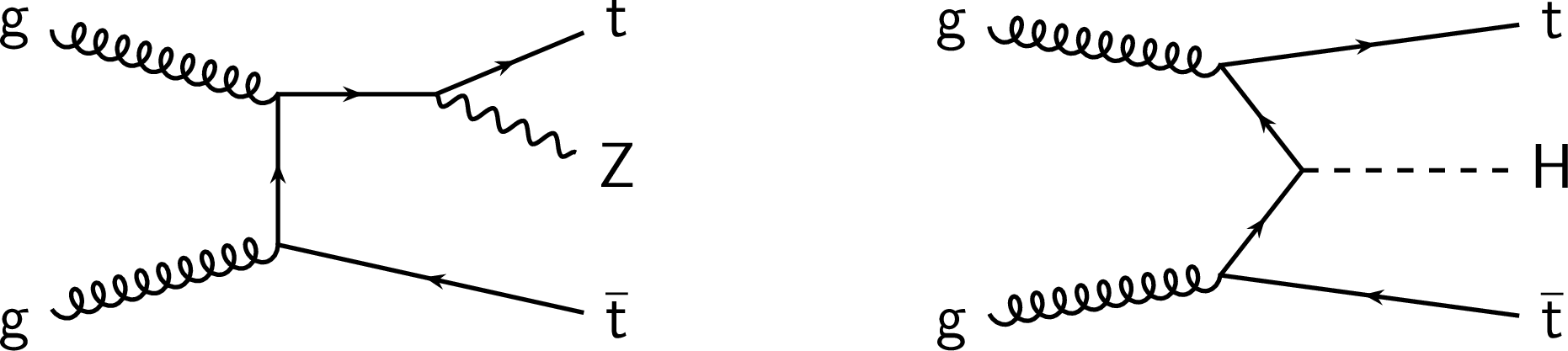
Figure 1:
Examples of tree-level Feynman diagrams for the $\mathrm{t\bar{t}}$Z (left) and $\mathrm{t\bar{t}}$H (right) production processes. |

png pdf |
Figure 1-a:
Examples of tree-level Feynman diagrams for the $\mathrm{t\bar{t}}$Z (left) and $\mathrm{t\bar{t}}$H (right) production processes. |
png pdf |
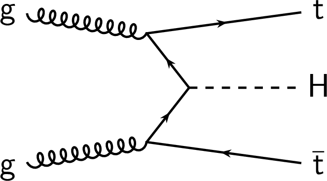
Figure 1-b:
Examples of tree-level Feynman diagrams for the $\mathrm{t\bar{t}}$Z (left) and $\mathrm{t\bar{t}}$H (right) production processes. |
png pdf |
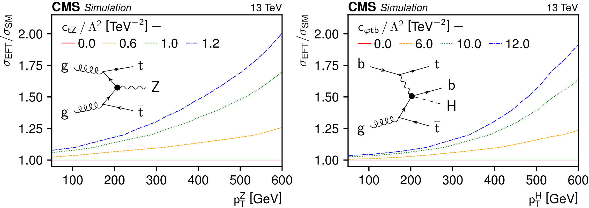
Figure 2:
The $\mathrm{t\bar{t}}$Z (left) and $\mathrm{t\bar{t}}$H (right) cross sections in the SM EFT, as ratios to the corresponding SM cross sections, as functions of $ {c_{\mathrm{t} \mathrm{Z}}} /{\Lambda}^{2}$ and the Z boson ${p_{\mathrm {T}}}$ (left), and $ {c_{\varphi \mathrm{t} \mathrm{b}}} /{\Lambda}^{2}$ and the Higgs boson ${p_{\mathrm {T}}}$ (right), where ${c_{\mathrm{t} \mathrm{Z}}}$ and ${c_{\varphi \mathrm{t} \mathrm{b}}}$ are the WCs for the EFT operators ${O_{\mathrm{u} \mathrm{B}}^\mathrm {(ij)}}$ and ${O_{\varphi \mathrm{u} \mathrm{d}}^\mathrm {(ij)}}$, respectively [7]. Example Feynman diagrams, in which the vertices affected by ${c_{\mathrm{t} \mathrm{Z}}}$ and ${c_{\varphi \mathrm{t} \mathrm{b}}}$ are marked by a filled dot, are also displayed. |

png pdf |
Figure 2-a:
The $\mathrm{t\bar{t}}$Z (left) and $\mathrm{t\bar{t}}$H (right) cross sections in the SM EFT, as ratios to the corresponding SM cross sections, as functions of $ {c_{\mathrm{t} \mathrm{Z}}} /{\Lambda}^{2}$ and the Z boson ${p_{\mathrm {T}}}$ (left), and $ {c_{\varphi \mathrm{t} \mathrm{b}}} /{\Lambda}^{2}$ and the Higgs boson ${p_{\mathrm {T}}}$ (right), where ${c_{\mathrm{t} \mathrm{Z}}}$ and ${c_{\varphi \mathrm{t} \mathrm{b}}}$ are the WCs for the EFT operators ${O_{\mathrm{u} \mathrm{B}}^\mathrm {(ij)}}$ and ${O_{\varphi \mathrm{u} \mathrm{d}}^\mathrm {(ij)}}$, respectively [7]. Example Feynman diagrams, in which the vertices affected by ${c_{\mathrm{t} \mathrm{Z}}}$ and ${c_{\varphi \mathrm{t} \mathrm{b}}}$ are marked by a filled dot, are also displayed. |

png pdf |
Figure 2-b:
The $\mathrm{t\bar{t}}$Z (left) and $\mathrm{t\bar{t}}$H (right) cross sections in the SM EFT, as ratios to the corresponding SM cross sections, as functions of $ {c_{\mathrm{t} \mathrm{Z}}} /{\Lambda}^{2}$ and the Z boson ${p_{\mathrm {T}}}$ (left), and $ {c_{\varphi \mathrm{t} \mathrm{b}}} /{\Lambda}^{2}$ and the Higgs boson ${p_{\mathrm {T}}}$ (right), where ${c_{\mathrm{t} \mathrm{Z}}}$ and ${c_{\varphi \mathrm{t} \mathrm{b}}}$ are the WCs for the EFT operators ${O_{\mathrm{u} \mathrm{B}}^\mathrm {(ij)}}$ and ${O_{\varphi \mathrm{u} \mathrm{d}}^\mathrm {(ij)}}$, respectively [7]. Example Feynman diagrams, in which the vertices affected by ${c_{\mathrm{t} \mathrm{Z}}}$ and ${c_{\varphi \mathrm{t} \mathrm{b}}}$ are marked by a filled dot, are also displayed. |
png pdf |
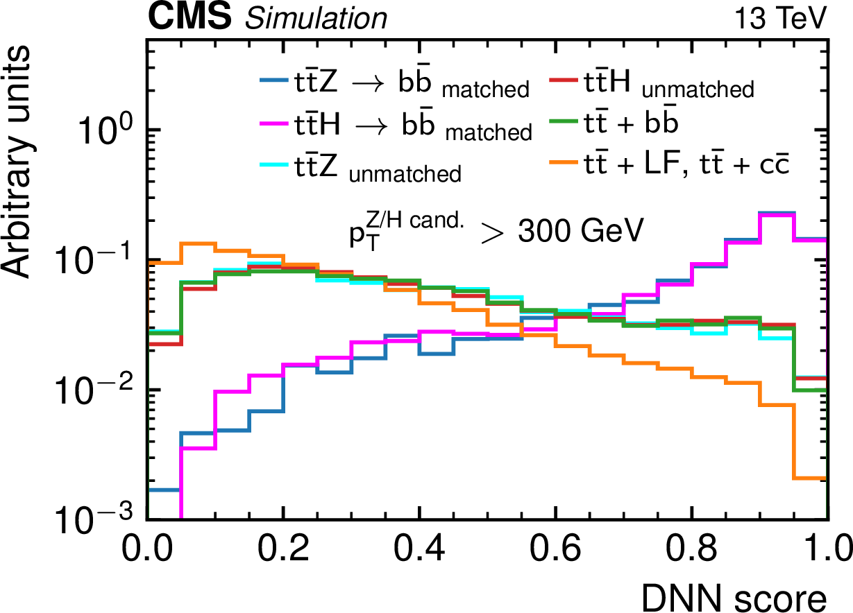
Figure 3:
The simulated DNN score distributions, normalized to unit area, for well-reconstructed $\mathrm{t\bar{t}}$Z and $\mathrm{t\bar{t}}$H signal events in which the reconstructed Z or Higgs boson candidate is matched to both generator-level b quark daughters of the Z or Higgs boson; the remaining $\mathrm{t\bar{t}}$Z and $\mathrm{t\bar{t}}$H events; background events from ${\mathrm{t} \mathrm{\bar{t}}}$ + $\mathrm{b} \mathrm{\bar{b}}$; and background events from ${\mathrm{t} \mathrm{\bar{t}}}$ +${\mathrm{c} \mathrm{\bar{c}}}$ and ${\mathrm{t} \mathrm{\bar{t}}}$ + LF. The events satisfy the baseline selection requirements described in Section 5 and contain a Z or Higgs boson candidate with $ {p_{\mathrm {T}}} > $ 300 GeV. |
png pdf |
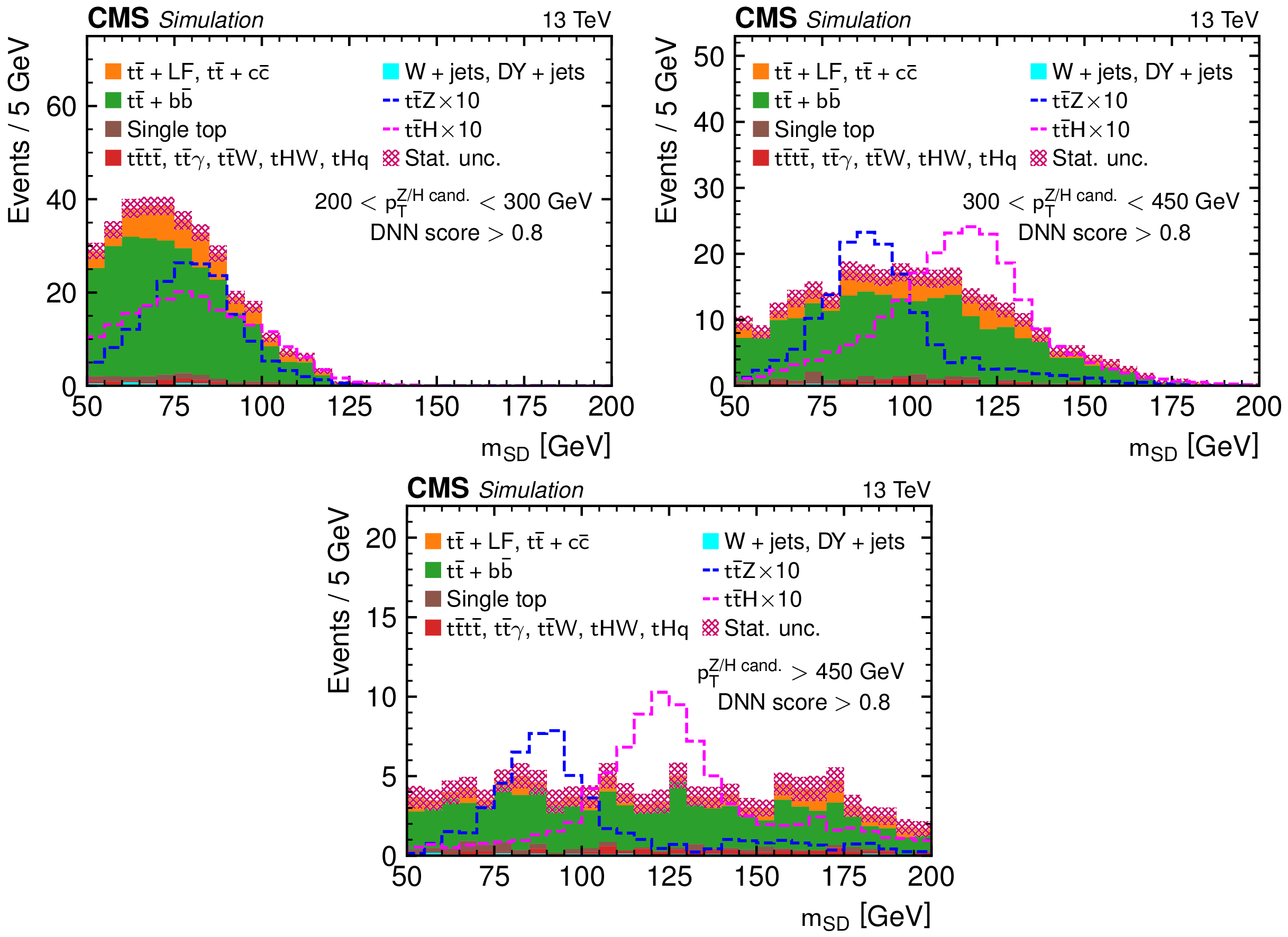
Figure 4:
Soft-drop mass distributions from simulation for background (solid histograms) and signal (dashed histograms) of $\mathrm{Z} /\mathrm{H} \to \mathrm{b} \mathrm{\bar{b}} $ candidate jets in three ${p_{\mathrm {T}}}$ ranges: 200-300 GeV (upper left), 300-450 GeV (upper right), and ${>}450 GeV $ (lower) in simulated samples with DNN score ${>} 0.8$. The signal distributions represent the SM prediction scaled up by a factor of 10 for easier comparison with the backgrounds. The signal distributions include well-reconstructed $\mathrm{t\bar{t}}$Z and $\mathrm{t\bar{t}}$H events as well as $\mathrm{t\bar{t}}$Z and $\mathrm{t\bar{t}}$H events that either do not contain Z/H $ \to \mathrm{b} \mathrm{\bar{b}} $ or are not well reconstructed. The red hatched bands correspond to the statistical uncertainty in the background. |
png pdf |
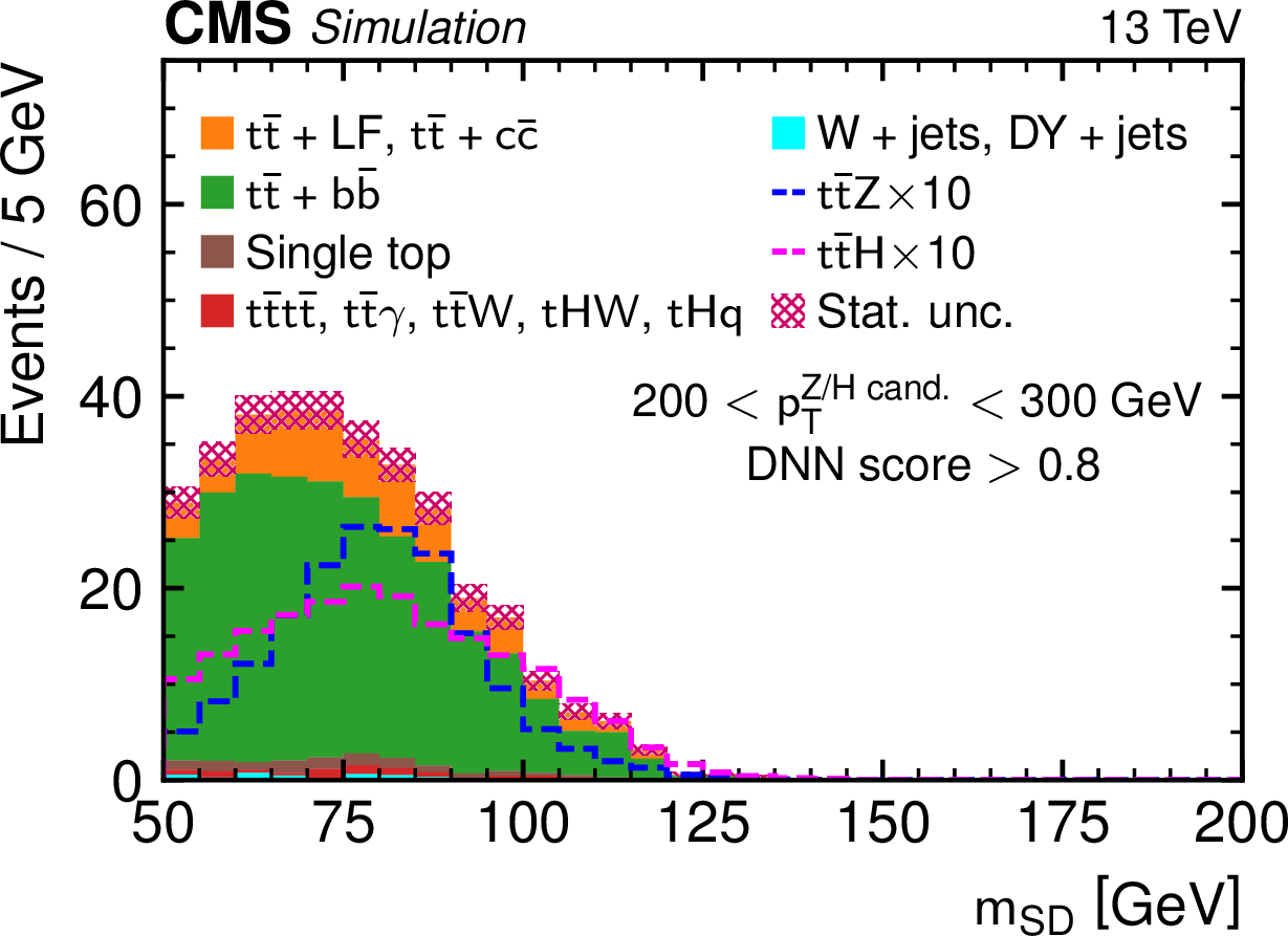
Figure 4-a:
Soft-drop mass distributions from simulation for background (solid histograms) and signal (dashed histograms) of $\mathrm{Z} /\mathrm{H} \to \mathrm{b} \mathrm{\bar{b}} $ candidate jets in three ${p_{\mathrm {T}}}$ ranges: 200-300 GeV (upper left), 300-450 GeV (upper right), and ${>}450 GeV $ (lower) in simulated samples with DNN score ${>} 0.8$. The signal distributions represent the SM prediction scaled up by a factor of 10 for easier comparison with the backgrounds. The signal distributions include well-reconstructed $\mathrm{t\bar{t}}$Z and $\mathrm{t\bar{t}}$H events as well as $\mathrm{t\bar{t}}$Z and $\mathrm{t\bar{t}}$H events that either do not contain Z/H $ \to \mathrm{b} \mathrm{\bar{b}} $ or are not well reconstructed. The red hatched bands correspond to the statistical uncertainty in the background. |
png pdf |
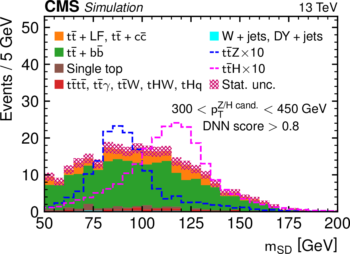
Figure 4-b:
Soft-drop mass distributions from simulation for background (solid histograms) and signal (dashed histograms) of $\mathrm{Z} /\mathrm{H} \to \mathrm{b} \mathrm{\bar{b}} $ candidate jets in three ${p_{\mathrm {T}}}$ ranges: 200-300 GeV (upper left), 300-450 GeV (upper right), and ${>}450 GeV $ (lower) in simulated samples with DNN score ${>} 0.8$. The signal distributions represent the SM prediction scaled up by a factor of 10 for easier comparison with the backgrounds. The signal distributions include well-reconstructed $\mathrm{t\bar{t}}$Z and $\mathrm{t\bar{t}}$H events as well as $\mathrm{t\bar{t}}$Z and $\mathrm{t\bar{t}}$H events that either do not contain Z/H $ \to \mathrm{b} \mathrm{\bar{b}} $ or are not well reconstructed. The red hatched bands correspond to the statistical uncertainty in the background. |
png pdf |
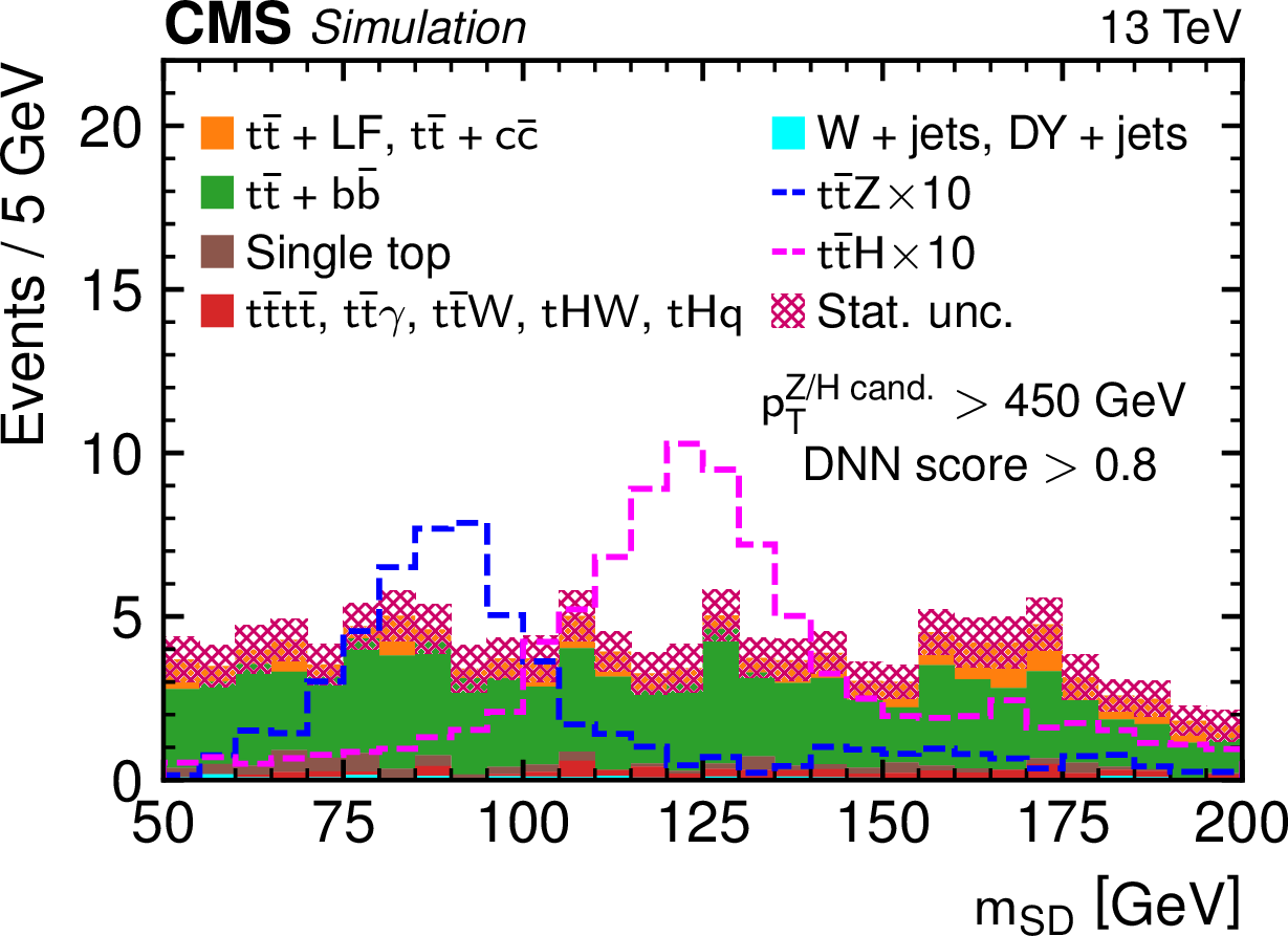
Figure 4-c:
Soft-drop mass distributions from simulation for background (solid histograms) and signal (dashed histograms) of $\mathrm{Z} /\mathrm{H} \to \mathrm{b} \mathrm{\bar{b}} $ candidate jets in three ${p_{\mathrm {T}}}$ ranges: 200-300 GeV (upper left), 300-450 GeV (upper right), and ${>}450 GeV $ (lower) in simulated samples with DNN score ${>} 0.8$. The signal distributions represent the SM prediction scaled up by a factor of 10 for easier comparison with the backgrounds. The signal distributions include well-reconstructed $\mathrm{t\bar{t}}$Z and $\mathrm{t\bar{t}}$H events as well as $\mathrm{t\bar{t}}$Z and $\mathrm{t\bar{t}}$H events that either do not contain Z/H $ \to \mathrm{b} \mathrm{\bar{b}} $ or are not well reconstructed. The red hatched bands correspond to the statistical uncertainty in the background. |
png pdf |
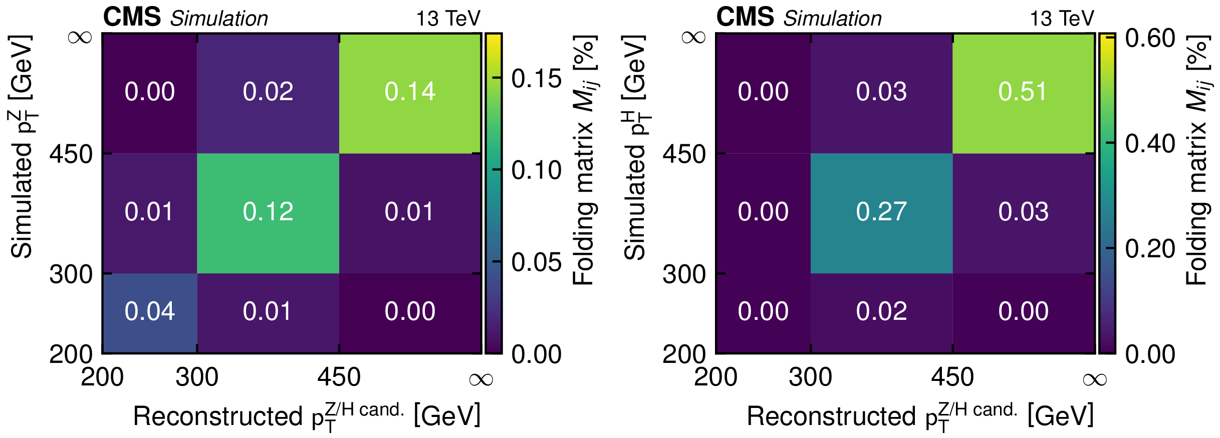
Figure 5:
The percentage of simulated $\mathrm{t\bar{t}}$Z (left) and $\mathrm{t\bar{t}}$H (right) signal events that satisfy the baseline event selection requirements as well as the DNN and mass requirements in bins defined by the reconstructed AK8 jet ${p_{\mathrm {T}}}$ ($x$ axis) and simulated $ {p_{\mathrm {T}}} ^{\mathrm{Z} /\mathrm{H}}$ ($y$ axis). The rightmost and uppermost bins are unbounded. The value of each bin is the ratio of the event yield in the bin to the total number of simulated signal events with a simulated $ {p_{\mathrm {T}}} ^{\mathrm{Z} /\mathrm{H}}$ in the same $y$-axis bin, including all decay modes of the top quark, Z boson, and Higgs boson. The color scale to the right shows the meaning of the histogram colors. |

png pdf |
Figure 5-a:
The percentage of simulated $\mathrm{t\bar{t}}$Z (left) and $\mathrm{t\bar{t}}$H (right) signal events that satisfy the baseline event selection requirements as well as the DNN and mass requirements in bins defined by the reconstructed AK8 jet ${p_{\mathrm {T}}}$ ($x$ axis) and simulated $ {p_{\mathrm {T}}} ^{\mathrm{Z} /\mathrm{H}}$ ($y$ axis). The rightmost and uppermost bins are unbounded. The value of each bin is the ratio of the event yield in the bin to the total number of simulated signal events with a simulated $ {p_{\mathrm {T}}} ^{\mathrm{Z} /\mathrm{H}}$ in the same $y$-axis bin, including all decay modes of the top quark, Z boson, and Higgs boson. The color scale to the right shows the meaning of the histogram colors. |
png pdf |
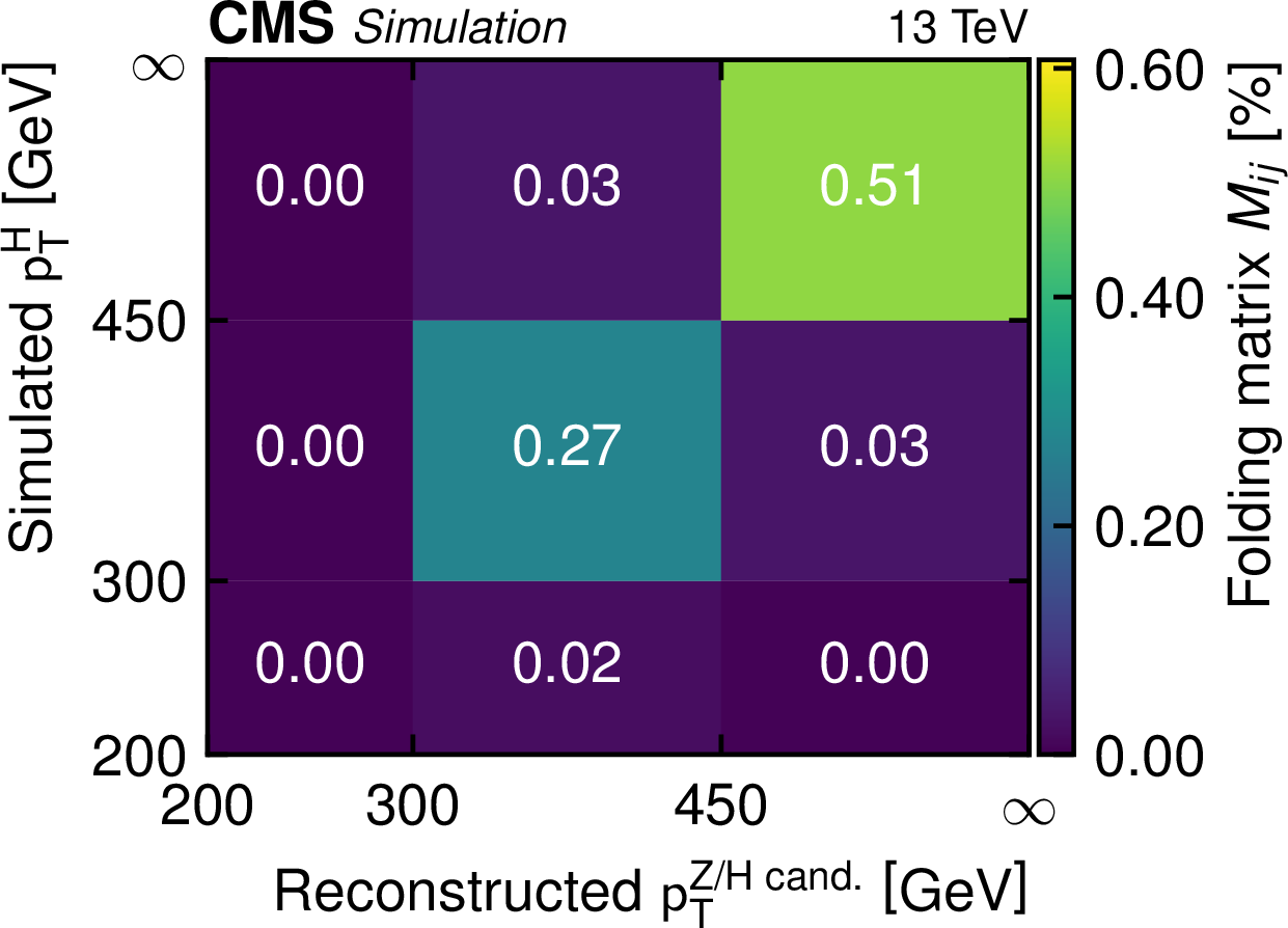
Figure 5-b:
The percentage of simulated $\mathrm{t\bar{t}}$Z (left) and $\mathrm{t\bar{t}}$H (right) signal events that satisfy the baseline event selection requirements as well as the DNN and mass requirements in bins defined by the reconstructed AK8 jet ${p_{\mathrm {T}}}$ ($x$ axis) and simulated $ {p_{\mathrm {T}}} ^{\mathrm{Z} /\mathrm{H}}$ ($y$ axis). The rightmost and uppermost bins are unbounded. The value of each bin is the ratio of the event yield in the bin to the total number of simulated signal events with a simulated $ {p_{\mathrm {T}}} ^{\mathrm{Z} /\mathrm{H}}$ in the same $y$-axis bin, including all decay modes of the top quark, Z boson, and Higgs boson. The color scale to the right shows the meaning of the histogram colors. |
png pdf |
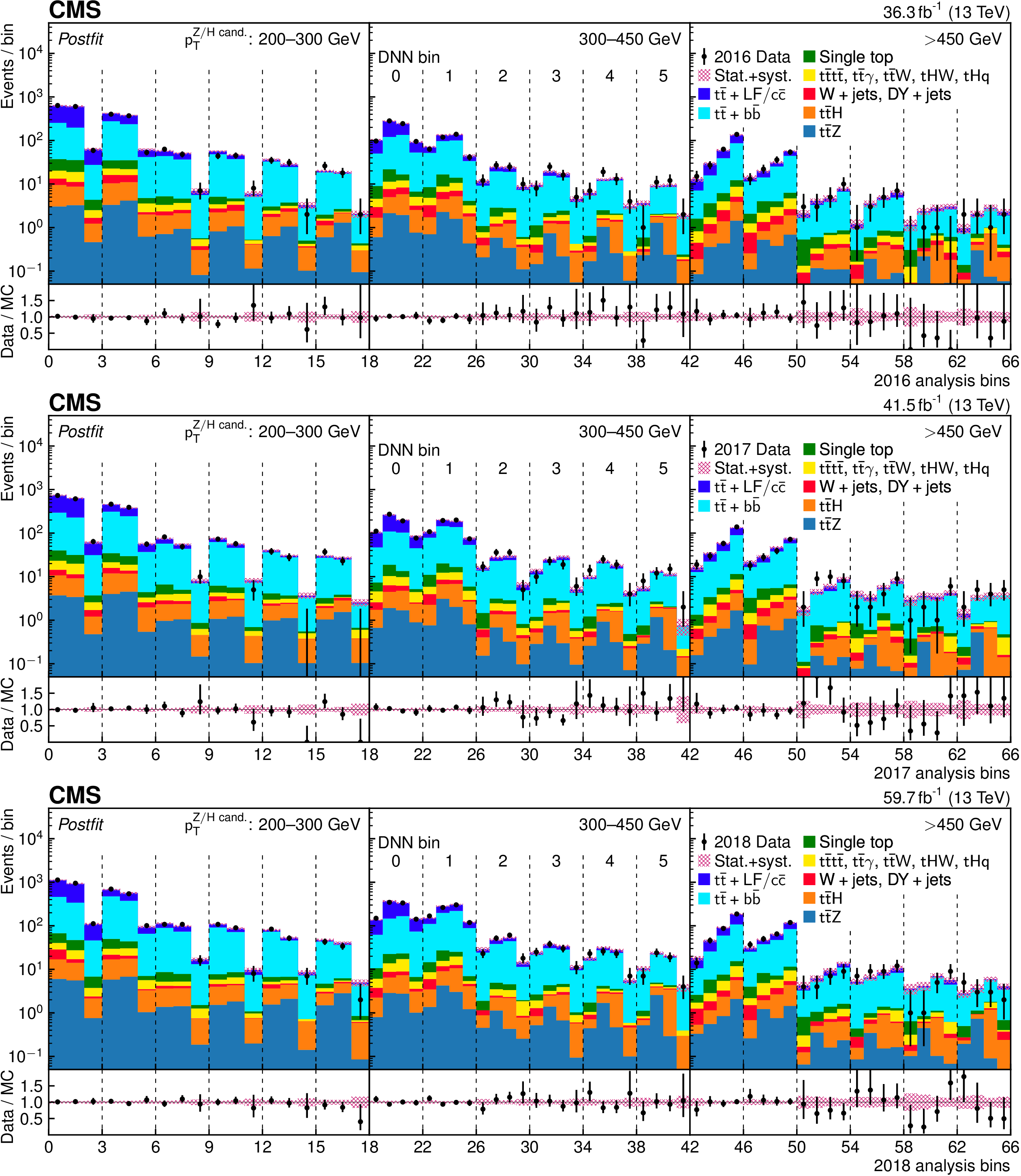
Figure 6:
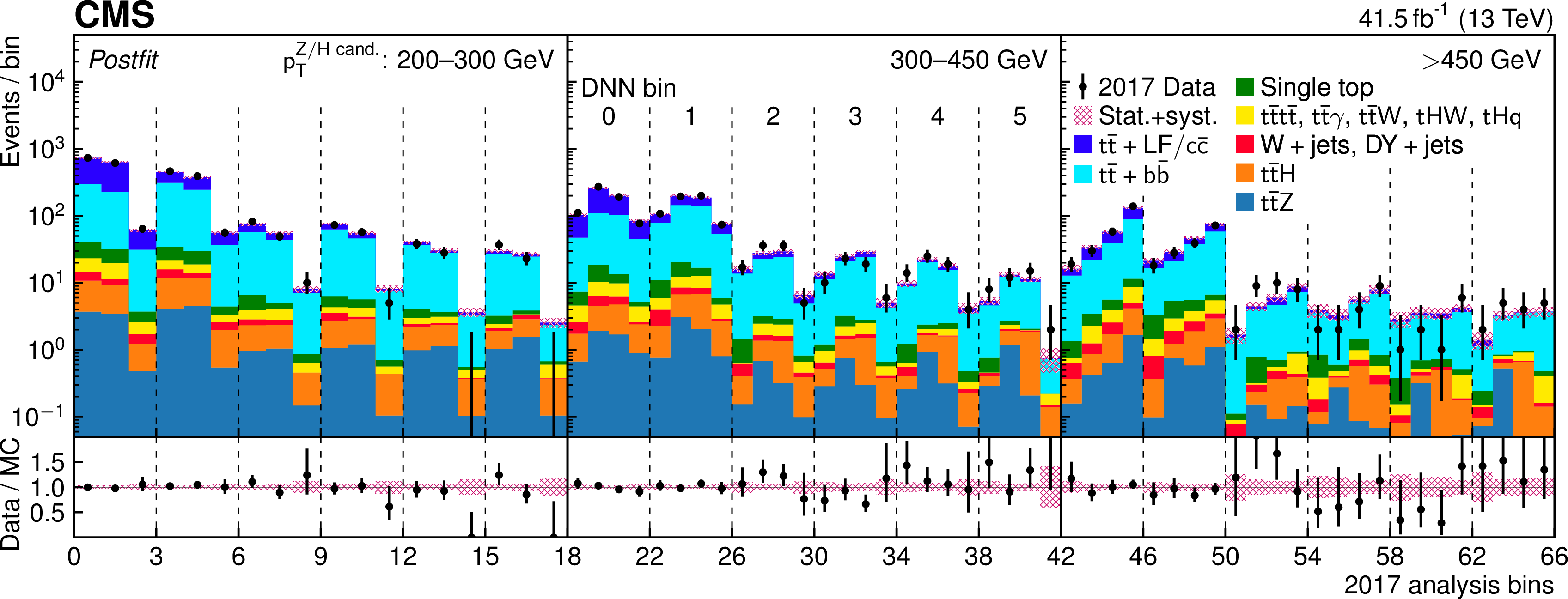
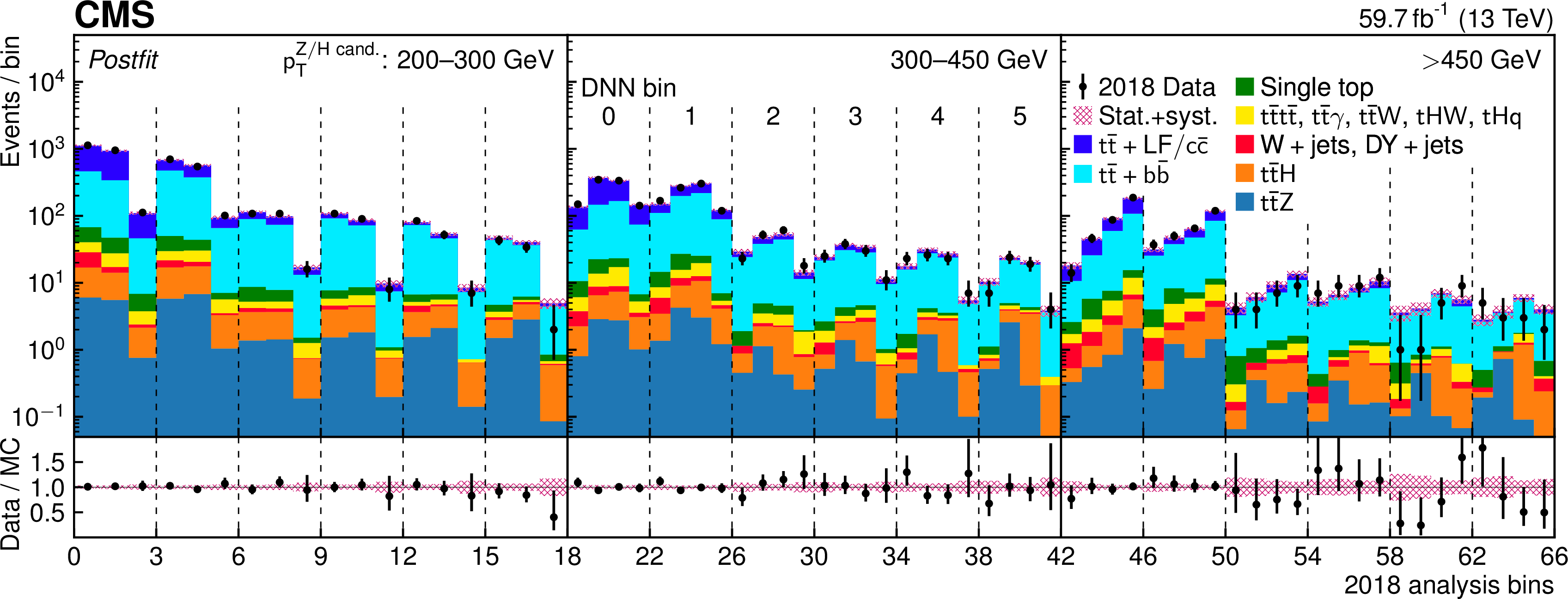
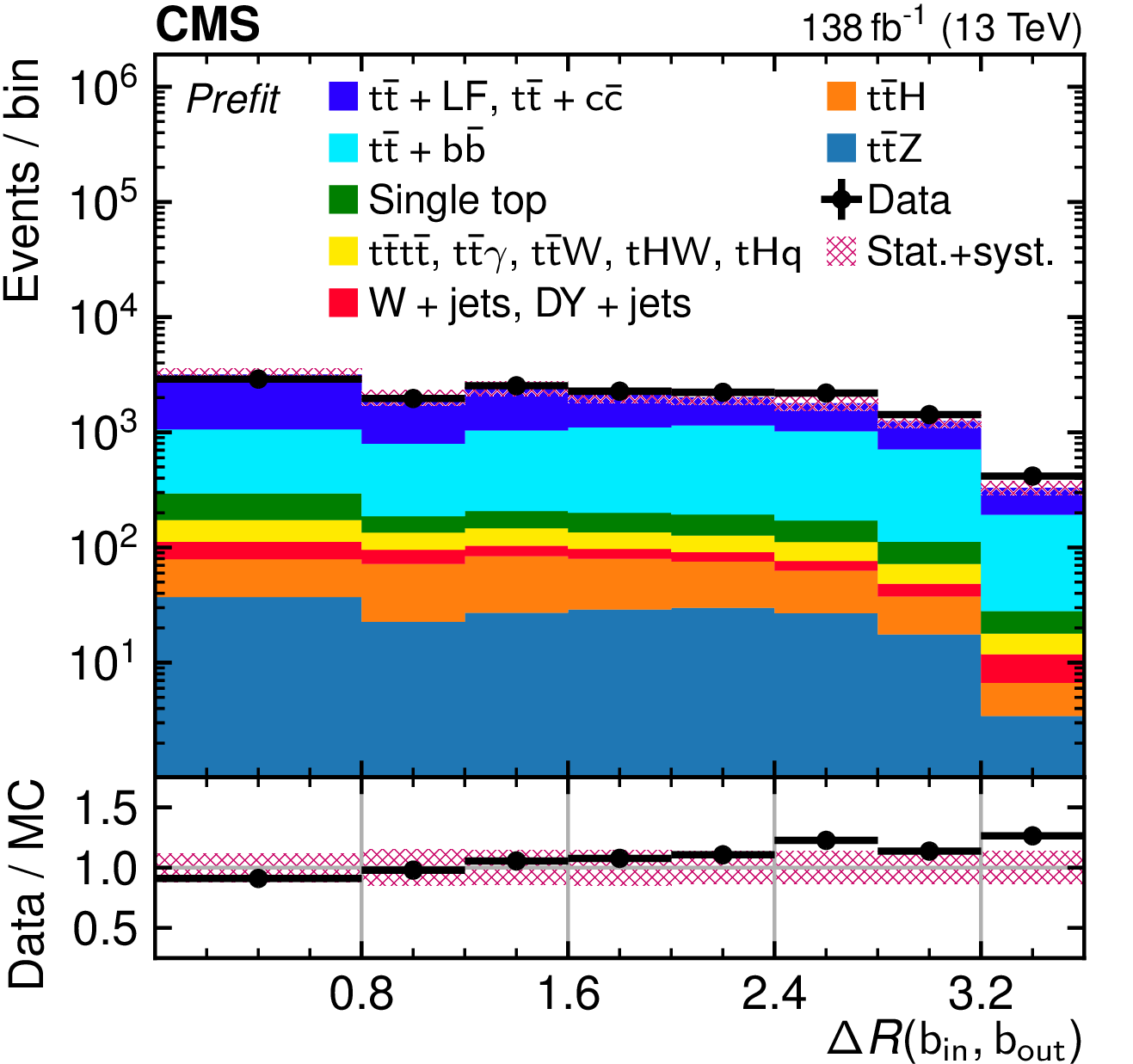
Postfit expected (solid histograms) and observed (points) yields for the 2016 (upper), 2017 (middle), and 2018 (lower) data-taking periods in each analysis bin. In the fit, the $\mathrm{t\bar{t}}$Z and $\mathrm{t\bar{t}}$H signal cross sections are fixed to the SM predictions. The analysis bins are defined as functions of the DNN score, and the ${p_{\mathrm {T}}}$ and ${m_\text {SD}}$ of the boson candidate AK8 jet. The largest three groupings of bins in each year are defined by the AK8 jet ${p_{\mathrm {T}}}$. The next six groups are defined by the DNN score, and the smallest groups of three or four bins with the same ${p_{\mathrm {T}}}$ and DNN score correspond to the AK8 jet ${m_\text {SD}}$. The vertical bars on the points show the statistical uncertainty in the data. The lower panels in each plot give the ratio of the data to the sum of the MC predictions, with the red band representing the total uncertainty in the MC prediction. |
png pdf |
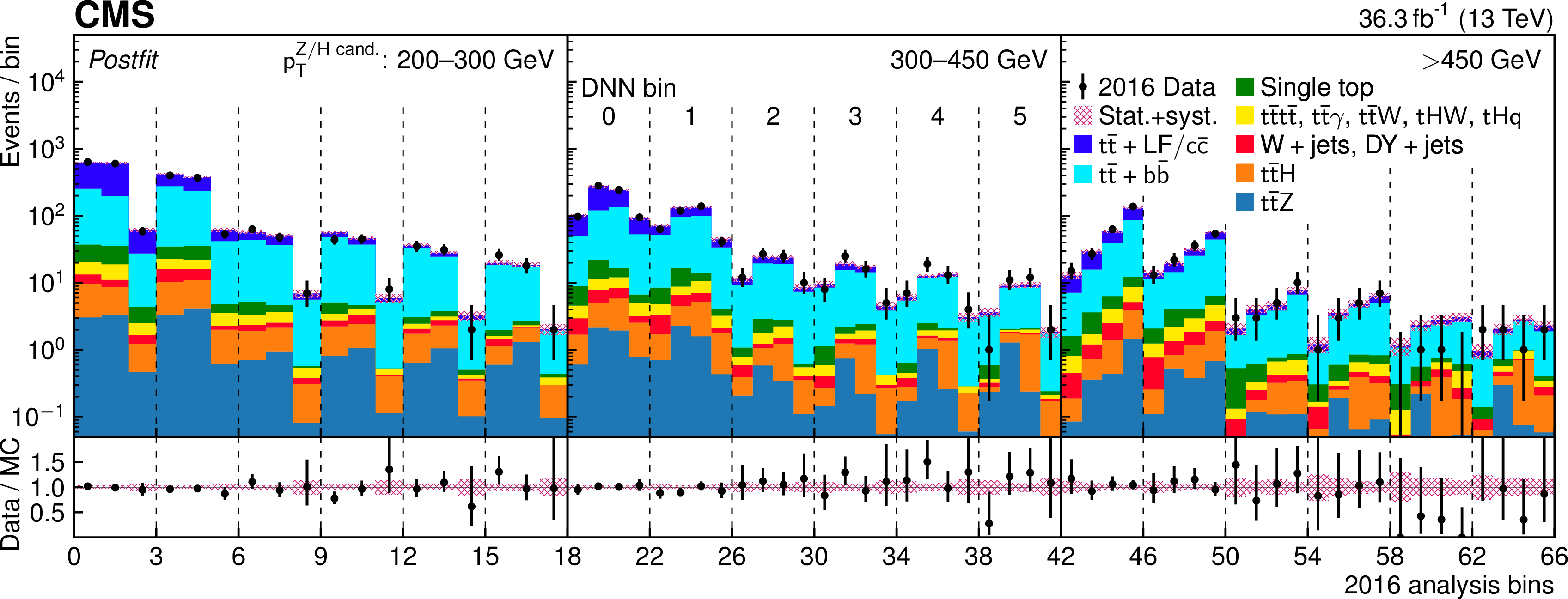
Figure 6-a:
Postfit expected (solid histograms) and observed (points) yields for the 2016 (upper), 2017 (middle), and 2018 (lower) data-taking periods in each analysis bin. In the fit, the $\mathrm{t\bar{t}}$Z and $\mathrm{t\bar{t}}$H signal cross sections are fixed to the SM predictions. The analysis bins are defined as functions of the DNN score, and the ${p_{\mathrm {T}}}$ and ${m_\text {SD}}$ of the boson candidate AK8 jet. The largest three groupings of bins in each year are defined by the AK8 jet ${p_{\mathrm {T}}}$. The next six groups are defined by the DNN score, and the smallest groups of three or four bins with the same ${p_{\mathrm {T}}}$ and DNN score correspond to the AK8 jet ${m_\text {SD}}$. The vertical bars on the points show the statistical uncertainty in the data. The lower panels in each plot give the ratio of the data to the sum of the MC predictions, with the red band representing the total uncertainty in the MC prediction. |
png pdf |
Figure 6-b:
Postfit expected (solid histograms) and observed (points) yields for the 2016 (upper), 2017 (middle), and 2018 (lower) data-taking periods in each analysis bin. In the fit, the $\mathrm{t\bar{t}}$Z and $\mathrm{t\bar{t}}$H signal cross sections are fixed to the SM predictions. The analysis bins are defined as functions of the DNN score, and the ${p_{\mathrm {T}}}$ and ${m_\text {SD}}$ of the boson candidate AK8 jet. The largest three groupings of bins in each year are defined by the AK8 jet ${p_{\mathrm {T}}}$. The next six groups are defined by the DNN score, and the smallest groups of three or four bins with the same ${p_{\mathrm {T}}}$ and DNN score correspond to the AK8 jet ${m_\text {SD}}$. The vertical bars on the points show the statistical uncertainty in the data. The lower panels in each plot give the ratio of the data to the sum of the MC predictions, with the red band representing the total uncertainty in the MC prediction. |
png pdf |
Figure 6-c:
Postfit expected (solid histograms) and observed (points) yields for the 2016 (upper), 2017 (middle), and 2018 (lower) data-taking periods in each analysis bin. In the fit, the $\mathrm{t\bar{t}}$Z and $\mathrm{t\bar{t}}$H signal cross sections are fixed to the SM predictions. The analysis bins are defined as functions of the DNN score, and the ${p_{\mathrm {T}}}$ and ${m_\text {SD}}$ of the boson candidate AK8 jet. The largest three groupings of bins in each year are defined by the AK8 jet ${p_{\mathrm {T}}}$. The next six groups are defined by the DNN score, and the smallest groups of three or four bins with the same ${p_{\mathrm {T}}}$ and DNN score correspond to the AK8 jet ${m_\text {SD}}$. The vertical bars on the points show the statistical uncertainty in the data. The lower panels in each plot give the ratio of the data to the sum of the MC predictions, with the red band representing the total uncertainty in the MC prediction. |
png pdf |
Figure 7:
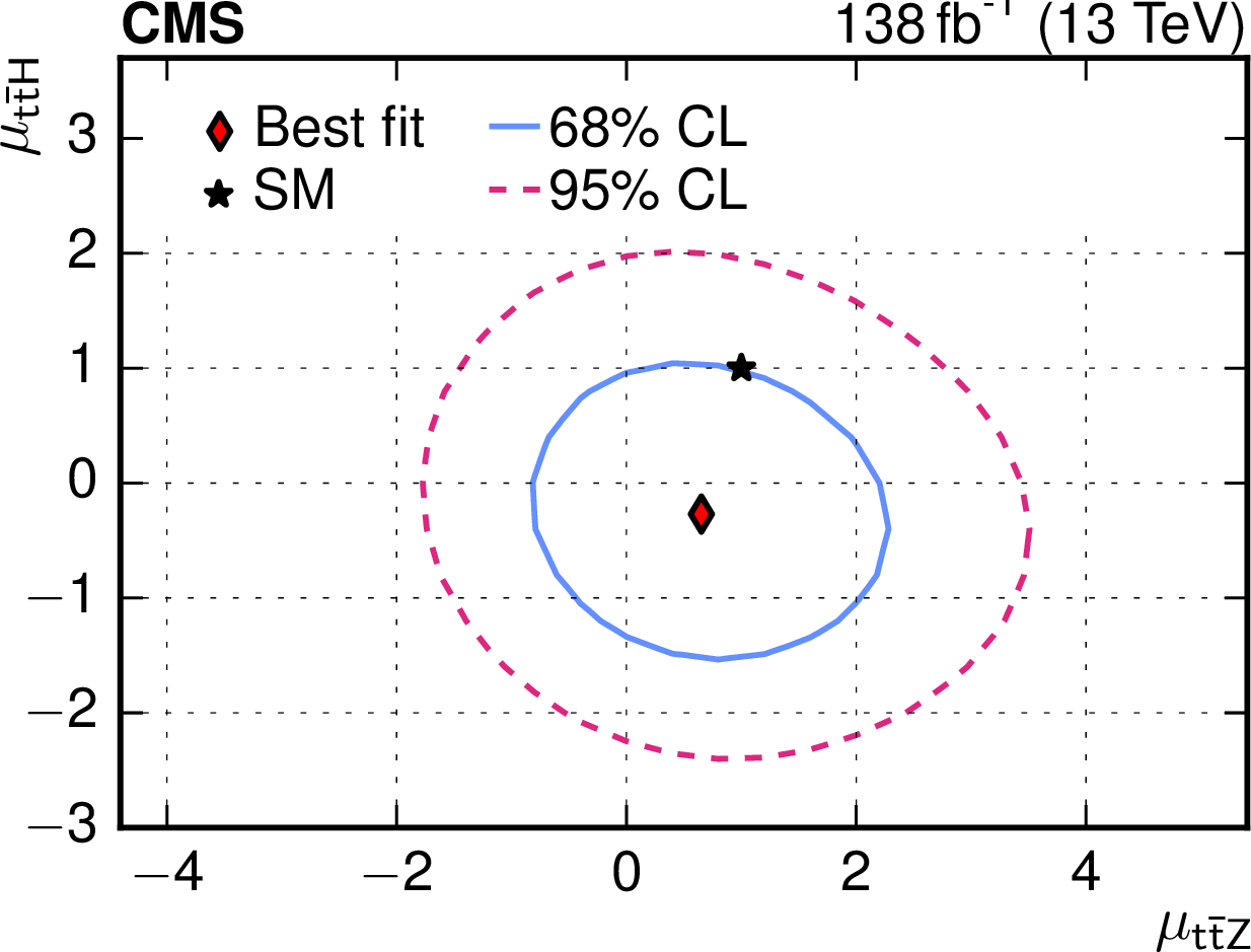
The observed best fit values (diamond) and SM predictions (star) for the signal strength modifiers $\mu _{{{\mathrm{t} \mathrm{\bar{t}}} \mathrm{H}}}$ versus $\mu _{{{\mathrm{t} \mathrm{\bar{t}}} \mathrm{Z}}}$ for generator-level $ {p_{\mathrm {T}}} ^{\mathrm{H}}$ or $ {p_{\mathrm {T}}} ^{\mathrm{Z}} > $ 200 GeV. The solid blue and dashed red contours show the 68 and 95% CL regions, respectively. |
png pdf |
Figure 8:
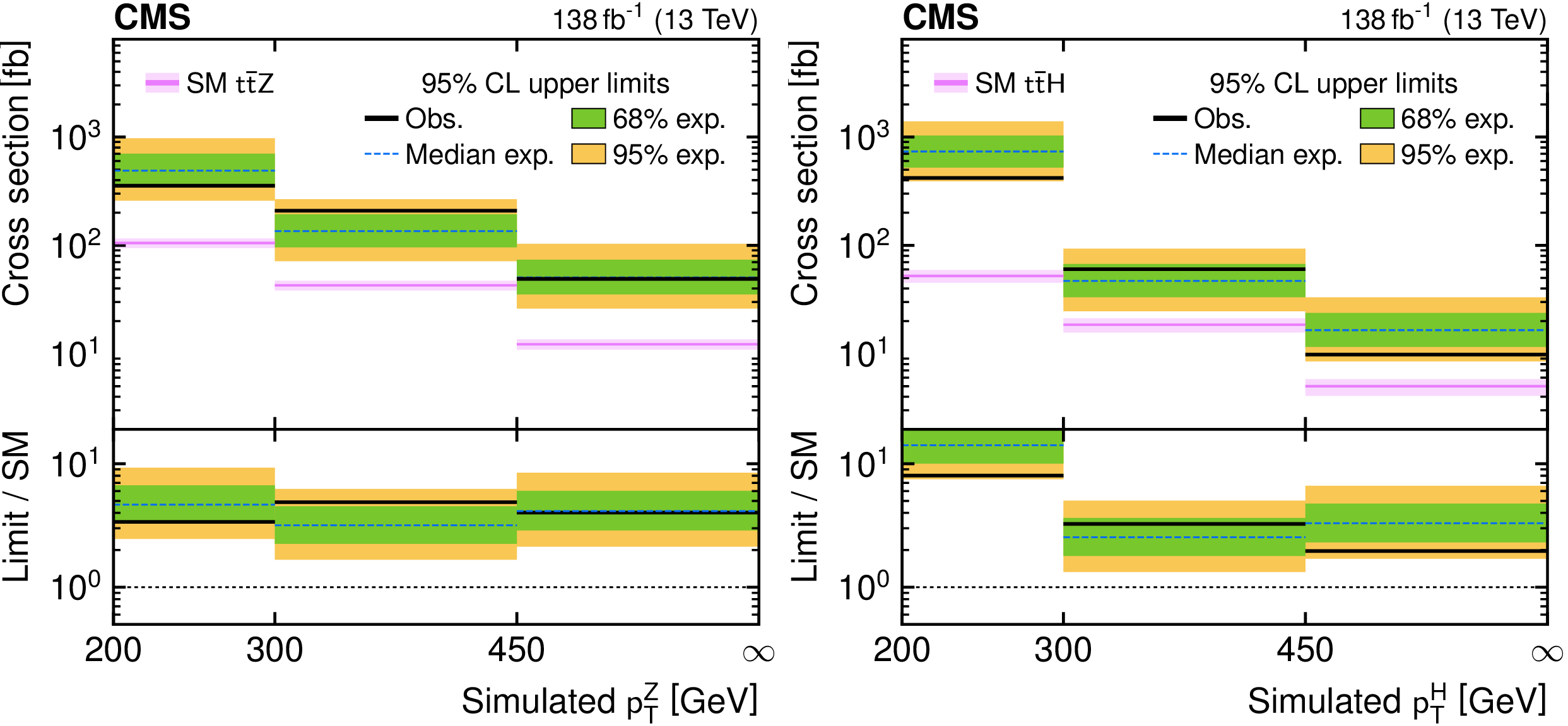
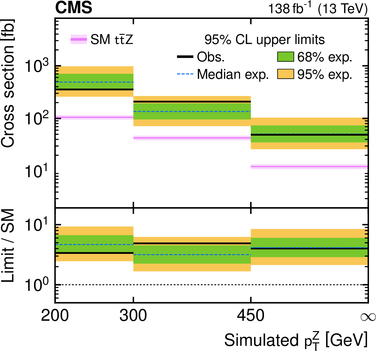
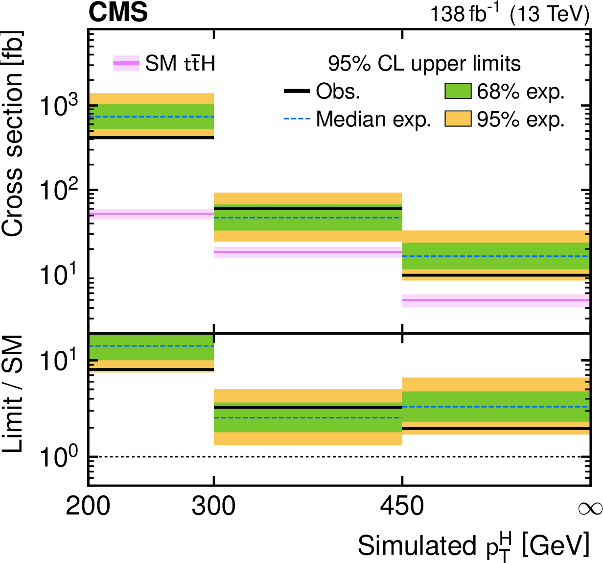
Observed and expected 95% CL upper limits on the $\mathrm{t\bar{t}}$Z (left) and $\mathrm{t\bar{t}}$H (right) differential cross sections as a function of the simulated Z and Higgs boson ${p_{\mathrm {T}}}$. The green and yellow bands indicate the regions containing 68 and 95%, respectively, of the distribution of limits under the SM hypothesis. The black lines represent the observed 95% CL upper limits. The magenta band shows the SM predicted differential cross sections with the PDF + ${\alpha _\mathrm {S}}$ and scale uncertainties. The lower panel shows the ratio of the observed and expected upper limits on the differential cross sections to the SM differential cross sections. The last bin is unbounded. |
png pdf |
Figure 8-a:
Observed and expected 95% CL upper limits on the $\mathrm{t\bar{t}}$Z (left) and $\mathrm{t\bar{t}}$H (right) differential cross sections as a function of the simulated Z and Higgs boson ${p_{\mathrm {T}}}$. The green and yellow bands indicate the regions containing 68 and 95%, respectively, of the distribution of limits under the SM hypothesis. The black lines represent the observed 95% CL upper limits. The magenta band shows the SM predicted differential cross sections with the PDF + ${\alpha _\mathrm {S}}$ and scale uncertainties. The lower panel shows the ratio of the observed and expected upper limits on the differential cross sections to the SM differential cross sections. The last bin is unbounded. |
png pdf |
Figure 8-b:
Observed and expected 95% CL upper limits on the $\mathrm{t\bar{t}}$Z (left) and $\mathrm{t\bar{t}}$H (right) differential cross sections as a function of the simulated Z and Higgs boson ${p_{\mathrm {T}}}$. The green and yellow bands indicate the regions containing 68 and 95%, respectively, of the distribution of limits under the SM hypothesis. The black lines represent the observed 95% CL upper limits. The magenta band shows the SM predicted differential cross sections with the PDF + ${\alpha _\mathrm {S}}$ and scale uncertainties. The lower panel shows the ratio of the observed and expected upper limits on the differential cross sections to the SM differential cross sections. The last bin is unbounded. |
png pdf |
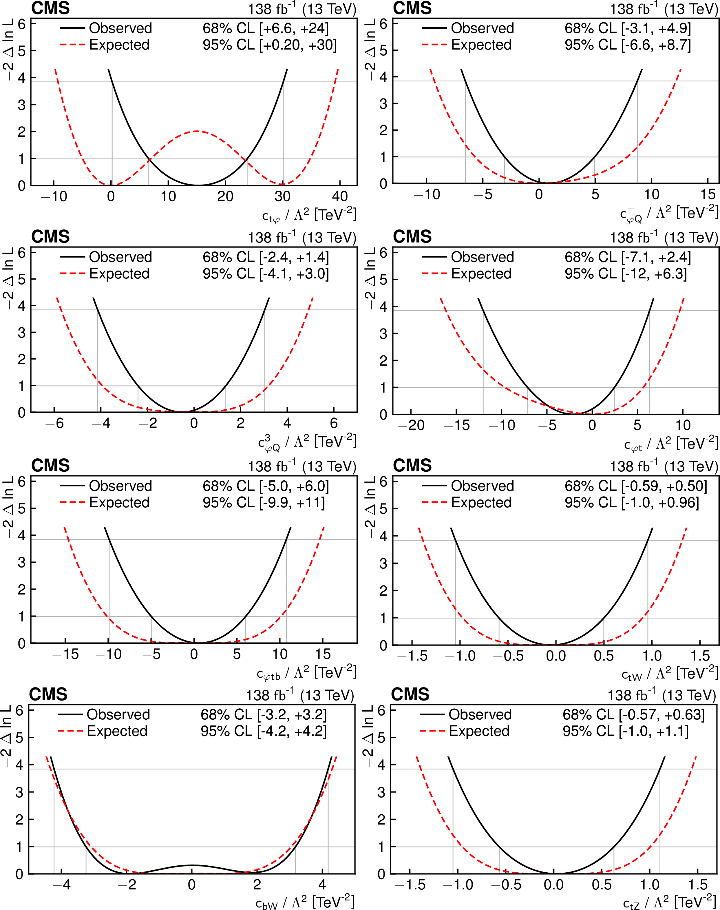
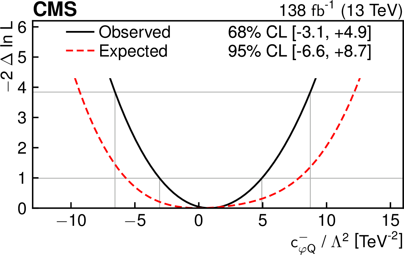
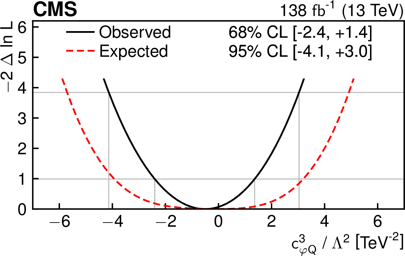
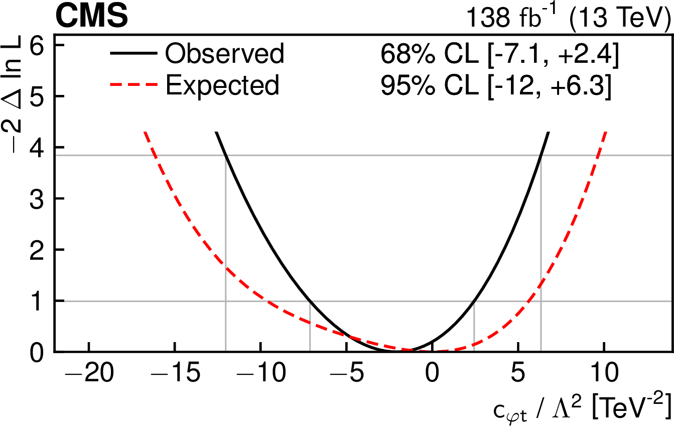
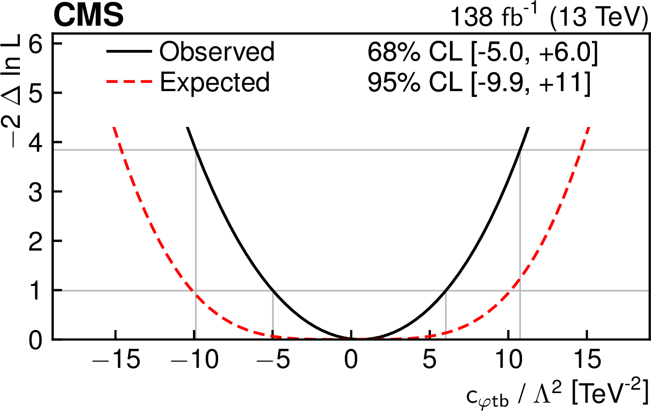
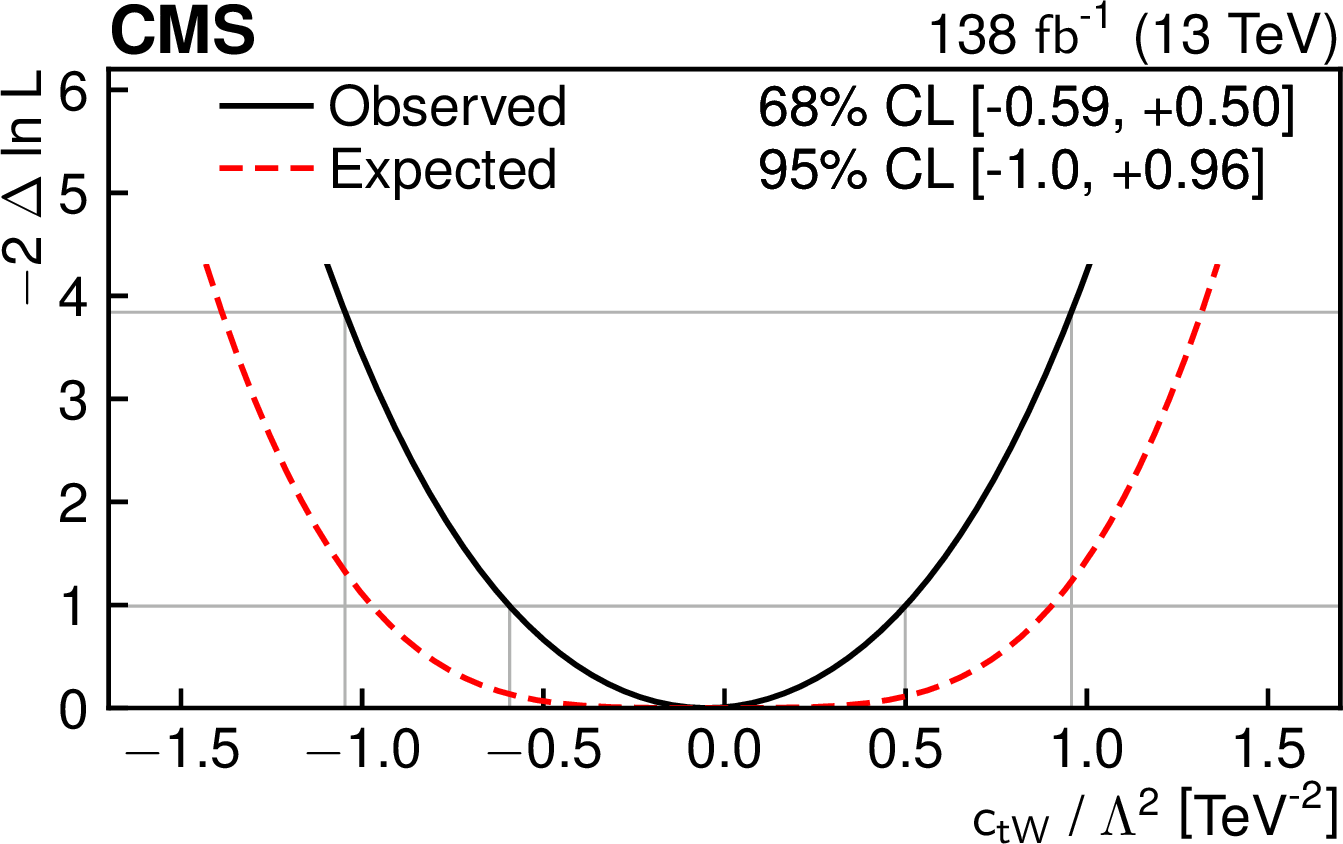
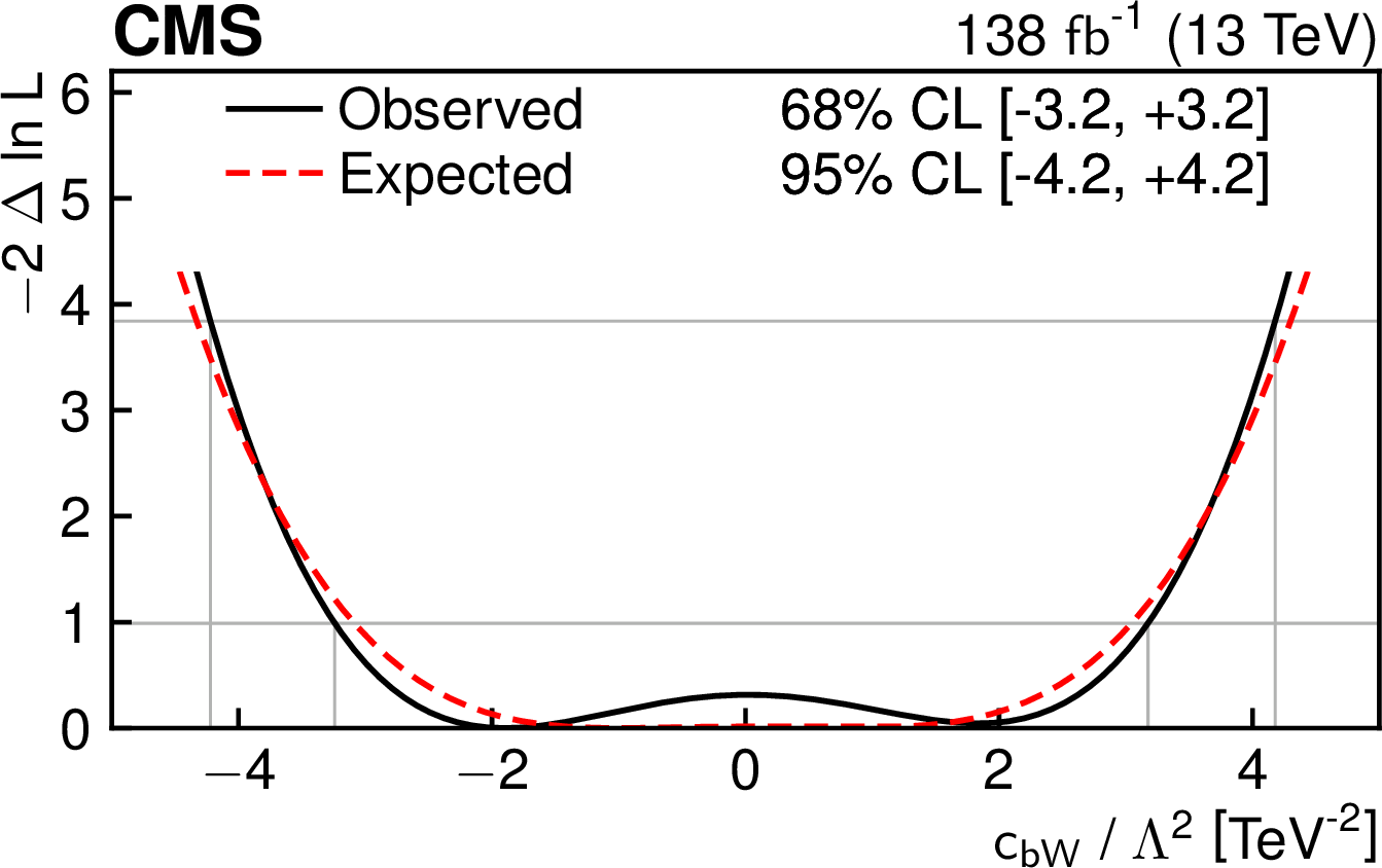
Figure 9:
Observed (solid black) and expected (dotted red) scans of the negative log-likelihood as a function of each of the eight WCs when the seven other WCs are fixed to their SM values. The 68 and 95% CL intervals are indicated by thin gray lines. |

png pdf |
Figure 9-a:
Observed (solid black) and expected (dotted red) scans of the negative log-likelihood as a function of each of the eight WCs when the seven other WCs are fixed to their SM values. The 68 and 95% CL intervals are indicated by thin gray lines. |
png pdf |
Figure 9-b:
Observed (solid black) and expected (dotted red) scans of the negative log-likelihood as a function of each of the eight WCs when the seven other WCs are fixed to their SM values. The 68 and 95% CL intervals are indicated by thin gray lines. |
png pdf |
Figure 9-c:
Observed (solid black) and expected (dotted red) scans of the negative log-likelihood as a function of each of the eight WCs when the seven other WCs are fixed to their SM values. The 68 and 95% CL intervals are indicated by thin gray lines. |
png pdf |
Figure 9-d:
Observed (solid black) and expected (dotted red) scans of the negative log-likelihood as a function of each of the eight WCs when the seven other WCs are fixed to their SM values. The 68 and 95% CL intervals are indicated by thin gray lines. |
png pdf |
Figure 9-e:
Observed (solid black) and expected (dotted red) scans of the negative log-likelihood as a function of each of the eight WCs when the seven other WCs are fixed to their SM values. The 68 and 95% CL intervals are indicated by thin gray lines. |
png pdf |
Figure 9-f:
Observed (solid black) and expected (dotted red) scans of the negative log-likelihood as a function of each of the eight WCs when the seven other WCs are fixed to their SM values. The 68 and 95% CL intervals are indicated by thin gray lines. |
png pdf |
Figure 9-g:
Observed (solid black) and expected (dotted red) scans of the negative log-likelihood as a function of each of the eight WCs when the seven other WCs are fixed to their SM values. The 68 and 95% CL intervals are indicated by thin gray lines. |

png pdf |
Figure 9-h:
Observed (solid black) and expected (dotted red) scans of the negative log-likelihood as a function of each of the eight WCs when the seven other WCs are fixed to their SM values. The 68 and 95% CL intervals are indicated by thin gray lines. |
png pdf |
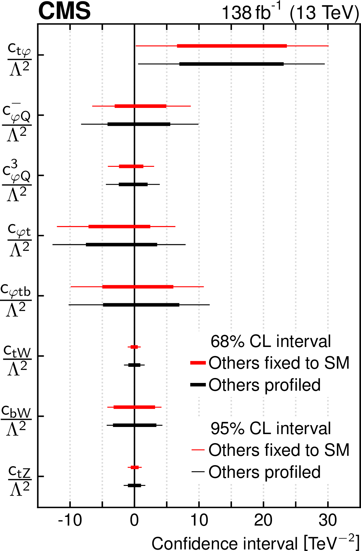
Figure 10:
The observed 68 and 95% CL intervals for the WCs are shown by the thick and thin bars, respectively. The intervals are found by scanning over a single WC while either profiling the other seven WCs (black) or fixing them to the SM value of zero (red). |
png pdf |
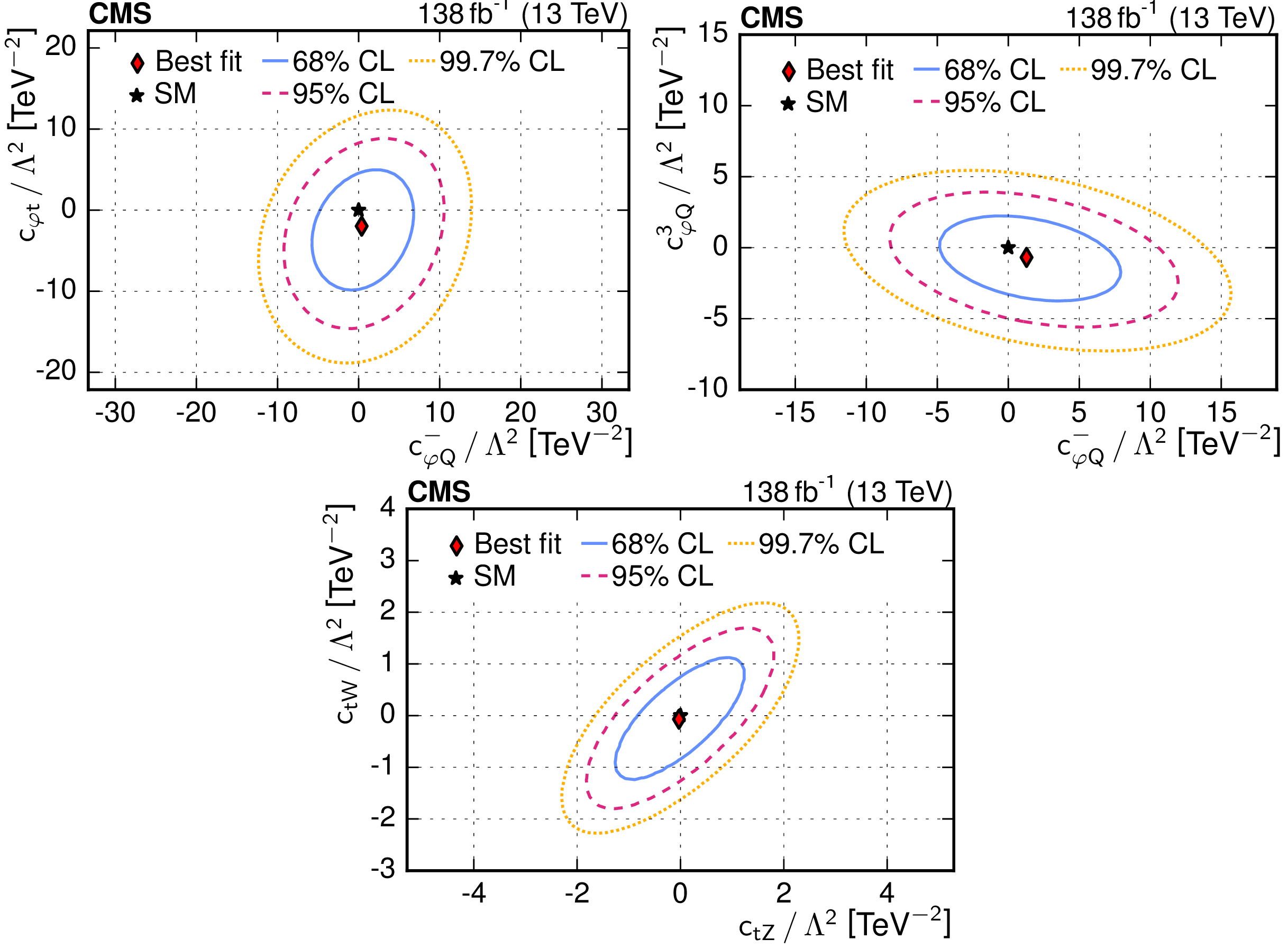
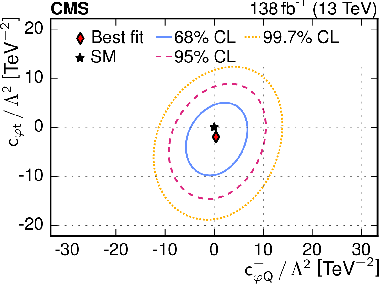
Figure 11:
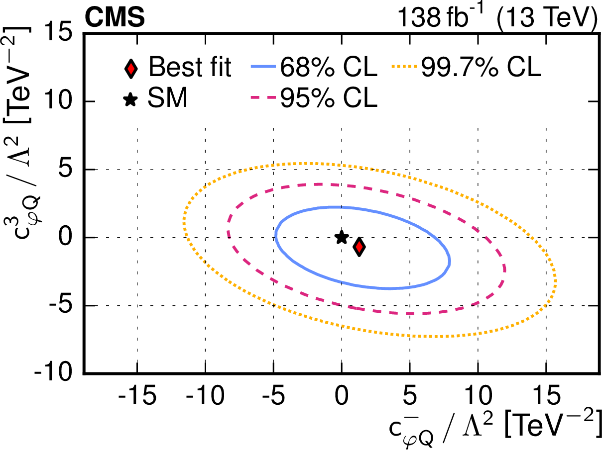
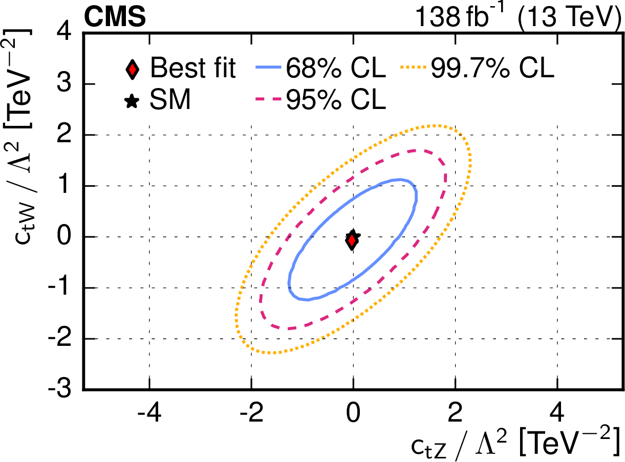
Observed two-dimensional scans of the negative log-likelihood as a function of two of the eight WCs when all other WCs are fixed to their SM values. The three pairs of WCs scanned have the three largest observed correlation coefficients among all pairs. They are ${c_{\varphi \mathrm{t}}}$ versus ${c^{-}_{\varphi \mathrm {Q}}}$ (upper left), ${c^{3}_{\varphi \mathrm {Q}}}$ versus ${c^{-}_{\varphi \mathrm {Q}}}$ (upper right), and ${c_{\mathrm{t} \mathrm{W}}}$ versus ${c_{\mathrm{t} \mathrm{Z}}}$ (lower). The 68, 95, and 99.7% CL intervals are indicated by the solid blue, dashed red, and dotted orange lines, respectively. |
png pdf |
Figure 11-a:
Observed two-dimensional scans of the negative log-likelihood as a function of two of the eight WCs when all other WCs are fixed to their SM values. The three pairs of WCs scanned have the three largest observed correlation coefficients among all pairs. They are ${c_{\varphi \mathrm{t}}}$ versus ${c^{-}_{\varphi \mathrm {Q}}}$ (upper left), ${c^{3}_{\varphi \mathrm {Q}}}$ versus ${c^{-}_{\varphi \mathrm {Q}}}$ (upper right), and ${c_{\mathrm{t} \mathrm{W}}}$ versus ${c_{\mathrm{t} \mathrm{Z}}}$ (lower). The 68, 95, and 99.7% CL intervals are indicated by the solid blue, dashed red, and dotted orange lines, respectively. |
png pdf |
Figure 11-b:
Observed two-dimensional scans of the negative log-likelihood as a function of two of the eight WCs when all other WCs are fixed to their SM values. The three pairs of WCs scanned have the three largest observed correlation coefficients among all pairs. They are ${c_{\varphi \mathrm{t}}}$ versus ${c^{-}_{\varphi \mathrm {Q}}}$ (upper left), ${c^{3}_{\varphi \mathrm {Q}}}$ versus ${c^{-}_{\varphi \mathrm {Q}}}$ (upper right), and ${c_{\mathrm{t} \mathrm{W}}}$ versus ${c_{\mathrm{t} \mathrm{Z}}}$ (lower). The 68, 95, and 99.7% CL intervals are indicated by the solid blue, dashed red, and dotted orange lines, respectively. |
png pdf |
Figure 11-c:
Observed two-dimensional scans of the negative log-likelihood as a function of two of the eight WCs when all other WCs are fixed to their SM values. The three pairs of WCs scanned have the three largest observed correlation coefficients among all pairs. They are ${c_{\varphi \mathrm{t}}}$ versus ${c^{-}_{\varphi \mathrm {Q}}}$ (upper left), ${c^{3}_{\varphi \mathrm {Q}}}$ versus ${c^{-}_{\varphi \mathrm {Q}}}$ (upper right), and ${c_{\mathrm{t} \mathrm{W}}}$ versus ${c_{\mathrm{t} \mathrm{Z}}}$ (lower). The 68, 95, and 99.7% CL intervals are indicated by the solid blue, dashed red, and dotted orange lines, respectively. |
png pdf |
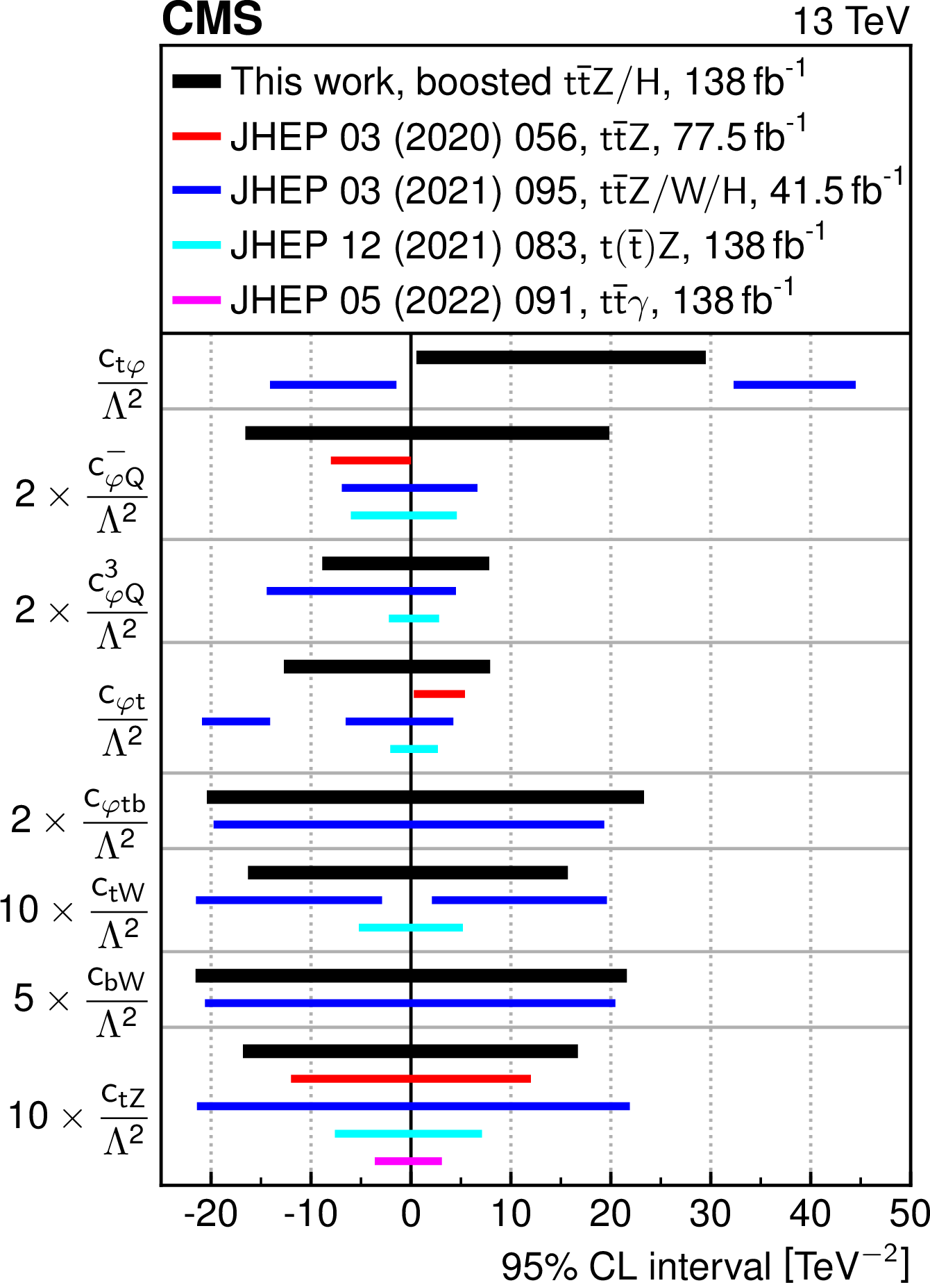
Figure 12:
Observed 95% CL intervals for the WCs. The intervals are found by scanning over a single WC while fixing the other seven to zero. For comparison, we also show the corresponding 95% CL intervals from Refs. [16,25,27,28], which used events with multiple leptons or photons. The intervals for several of the WCs would be too small to see clearly, and so we have increased their size by the factor given in the label on the left edge of the figure. |
png pdf |
Figure A1:
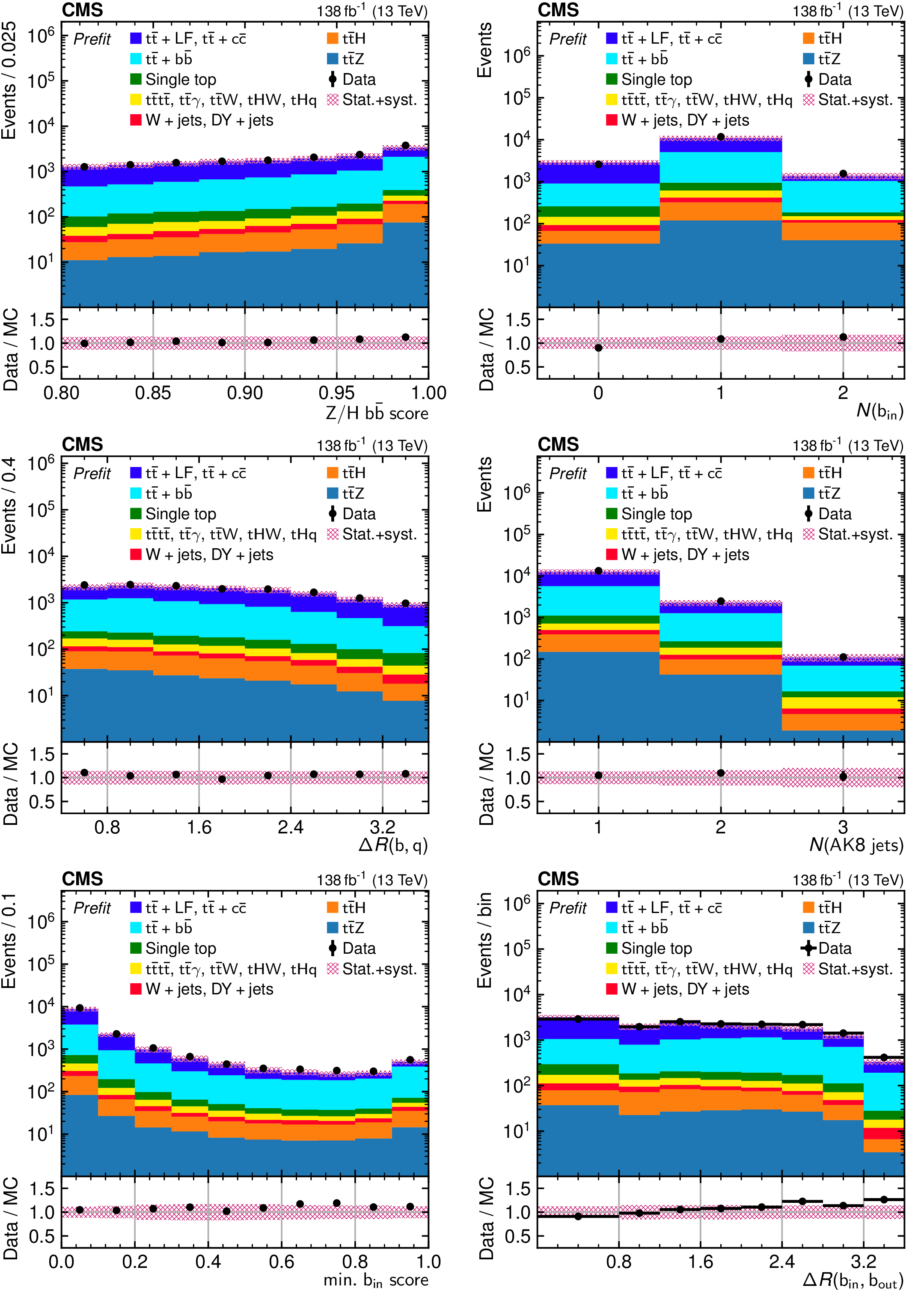
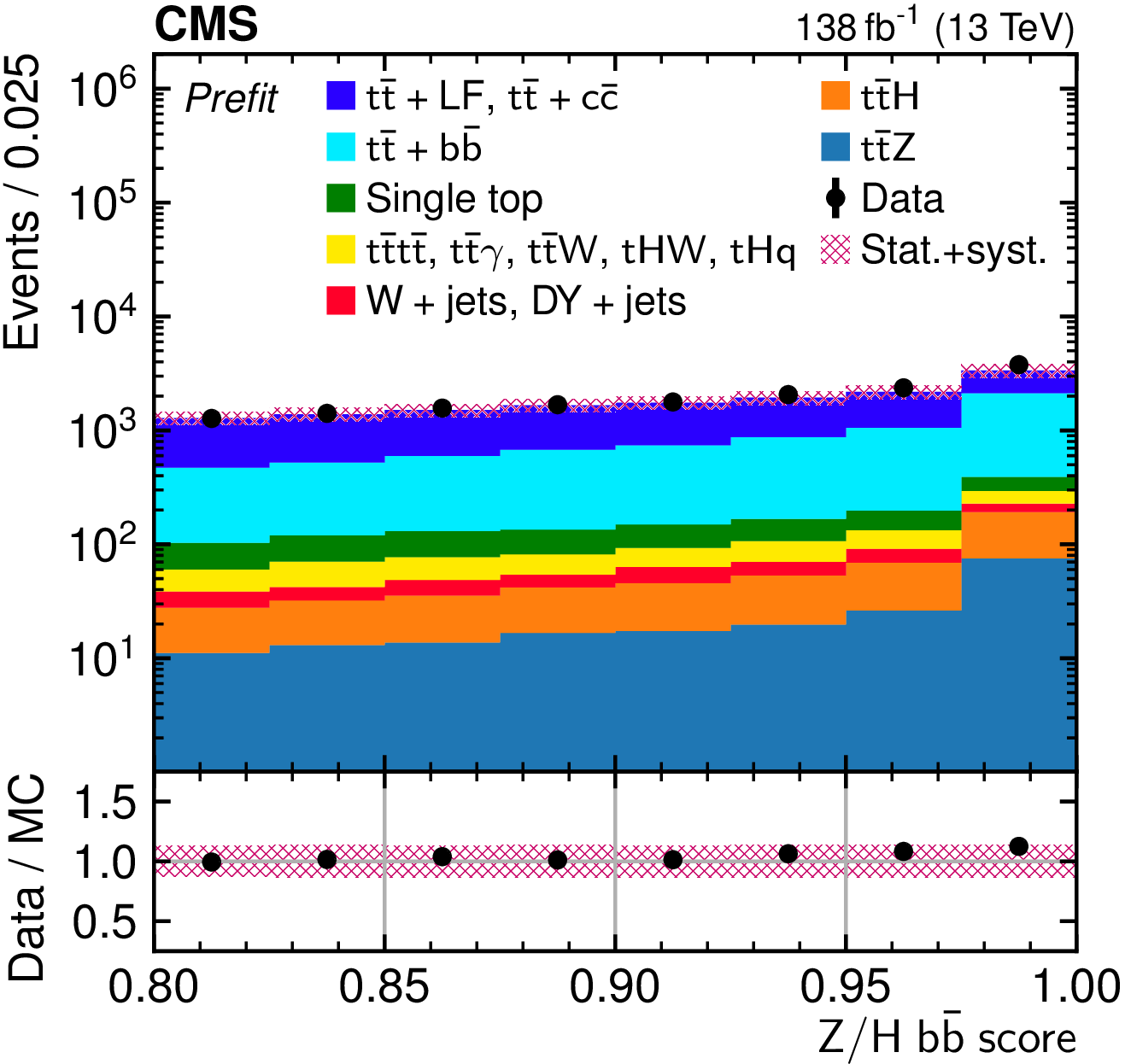
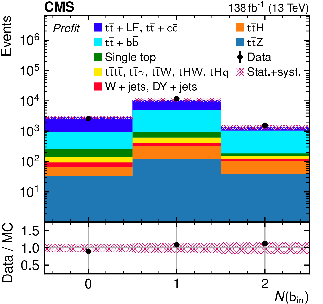
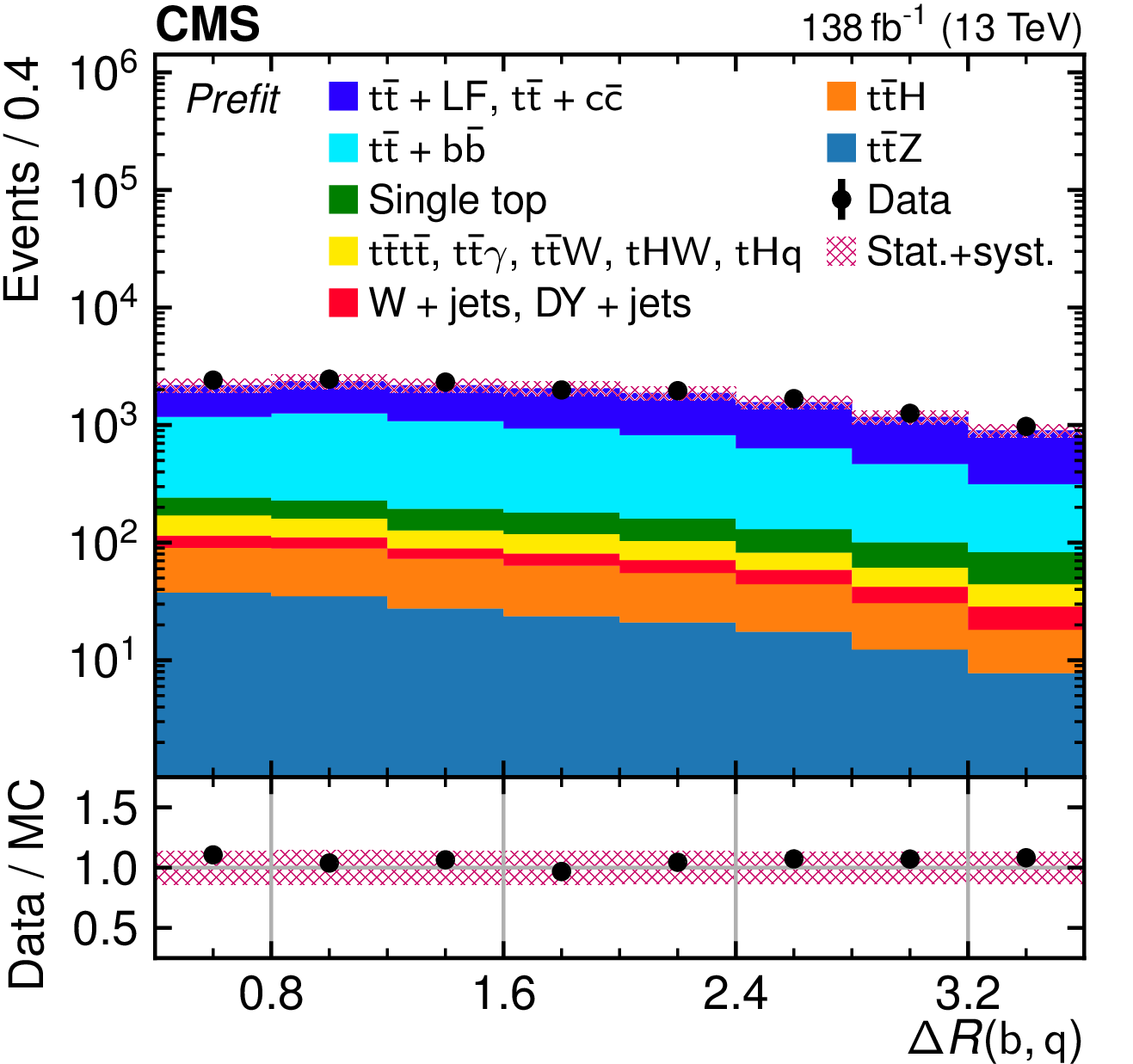
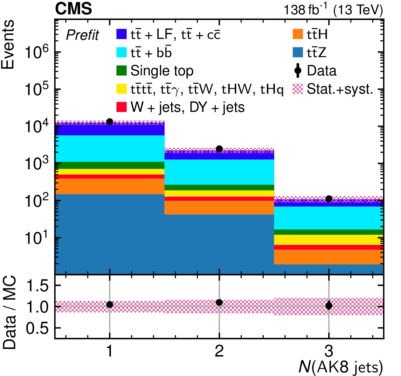
Prefit expected (colored histograms) and observed (point) distributions of selected DNN input variables, each of which is described in detail in Table A.1. These distributions represent the combined 2016-2018 data-taking periods. The hatched bands represent the total statistical and systematic uncertainty in the expected distributions, while the vertical bars on the black points indicate the statistical uncertainty in the observed distributions and the horizontal bars indicate the bin widths. The lower panels show the ratio of the observed yields to the sum of the MC predictions. |
png pdf |
Figure A1-a:
Prefit expected (colored histograms) and observed (point) distributions of selected DNN input variables, each of which is described in detail in Table A.1. These distributions represent the combined 2016-2018 data-taking periods. The hatched bands represent the total statistical and systematic uncertainty in the expected distributions, while the vertical bars on the black points indicate the statistical uncertainty in the observed distributions and the horizontal bars indicate the bin widths. The lower panels show the ratio of the observed yields to the sum of the MC predictions. |
png pdf |
Figure A1-b:
Prefit expected (colored histograms) and observed (point) distributions of selected DNN input variables, each of which is described in detail in Table A.1. These distributions represent the combined 2016-2018 data-taking periods. The hatched bands represent the total statistical and systematic uncertainty in the expected distributions, while the vertical bars on the black points indicate the statistical uncertainty in the observed distributions and the horizontal bars indicate the bin widths. The lower panels show the ratio of the observed yields to the sum of the MC predictions. |
png pdf |
Figure A1-c:
Prefit expected (colored histograms) and observed (point) distributions of selected DNN input variables, each of which is described in detail in Table A.1. These distributions represent the combined 2016-2018 data-taking periods. The hatched bands represent the total statistical and systematic uncertainty in the expected distributions, while the vertical bars on the black points indicate the statistical uncertainty in the observed distributions and the horizontal bars indicate the bin widths. The lower panels show the ratio of the observed yields to the sum of the MC predictions. |
png pdf |
Figure A1-d:
Prefit expected (colored histograms) and observed (point) distributions of selected DNN input variables, each of which is described in detail in Table A.1. These distributions represent the combined 2016-2018 data-taking periods. The hatched bands represent the total statistical and systematic uncertainty in the expected distributions, while the vertical bars on the black points indicate the statistical uncertainty in the observed distributions and the horizontal bars indicate the bin widths. The lower panels show the ratio of the observed yields to the sum of the MC predictions. |

png pdf |
Figure A1-e:
Prefit expected (colored histograms) and observed (point) distributions of selected DNN input variables, each of which is described in detail in Table A.1. These distributions represent the combined 2016-2018 data-taking periods. The hatched bands represent the total statistical and systematic uncertainty in the expected distributions, while the vertical bars on the black points indicate the statistical uncertainty in the observed distributions and the horizontal bars indicate the bin widths. The lower panels show the ratio of the observed yields to the sum of the MC predictions. |
png pdf |
Figure A1-f:
Prefit expected (colored histograms) and observed (point) distributions of selected DNN input variables, each of which is described in detail in Table A.1. These distributions represent the combined 2016-2018 data-taking periods. The hatched bands represent the total statistical and systematic uncertainty in the expected distributions, while the vertical bars on the black points indicate the statistical uncertainty in the observed distributions and the horizontal bars indicate the bin widths. The lower panels show the ratio of the observed yields to the sum of the MC predictions. |
| Tables | |
png pdf |
Table 1:
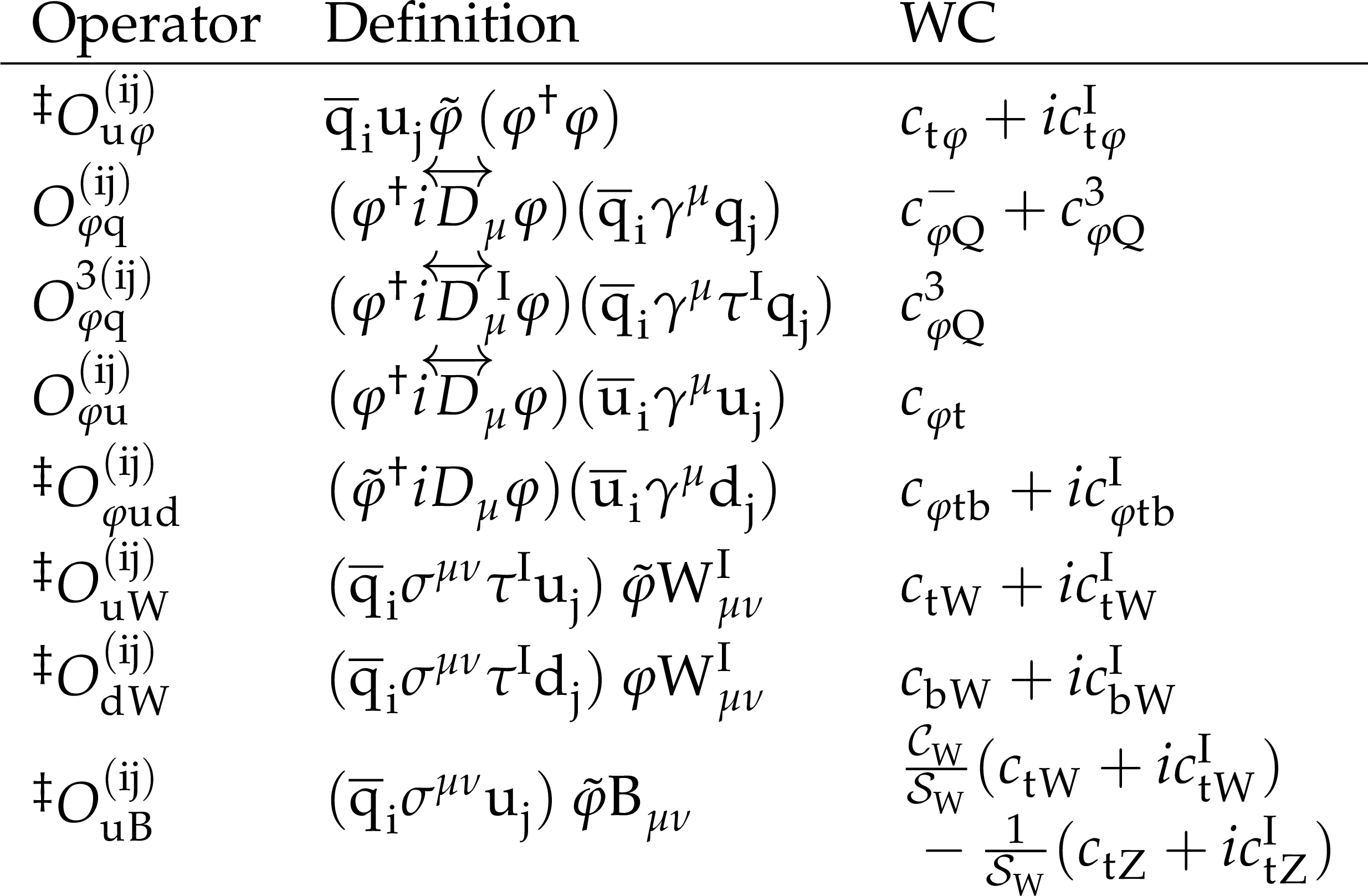
The set of EFT operators considered in this analysis that affect the $\mathrm{t\bar{t}}$Z and $\mathrm{t\bar{t}}$H processes at order $1/\Lambda ^2$. The couplings are restricted to involve only third-generation quarks. The symbol $\gamma ^\mu $ denotes the Dirac matrices and $\sigma ^{\mu \nu} \equiv i \left (\gamma ^\mu \gamma ^\nu - g^{\mu \nu}\right)$, where $g^{\mu \nu}$ is the metric tensor and $\tau ^\mathrm {I}$ are the Pauli matrices. The field $\varphi $ is the Higgs boson doublet and $\tilde{\varphi}^\mathrm {j} \equiv \varepsilon _\mathrm {jk} \left (\varphi ^\mathrm {k}\right)^*$, where $\varepsilon _\mathrm {jk}$ is the Levi-Civita symbol and $\varepsilon _{12} = +$1. The quark doublet and the right-handed quark singlets are represented by q, u, and d, respectively. The quantities ${(\varphi^\dagger i\!\overleftrightarrow{D}_{\!\!\mu}\varphi)} \equiv \varphi ^\dagger (iD_\mu \varphi)-(iD_\mu \varphi ^\dagger)\varphi $ and ${(\varphi^\dagger i\!\overleftrightarrow{D}^\mathrm{I}_{\!\!\mu}\varphi)} \equiv \varphi ^{\dagger}\tau ^\mathrm {I}(iD_\mu \varphi)-(iD_\mu \varphi ^\dagger)\tau ^\mathrm {I}\varphi $, where $D_{\mu}$ is the covariant derivative. The symbols $\mathrm{W} _{\mu \nu}^\mathrm {I}$ and $\mathrm{B} _{\mu \nu}$ are the field strength tensors for the weak isospin and weak hypercharge gauge fields. The abbreviations ${\mathcal {S}_{\mathrm {W}}}$ and ${\mathcal {C}_{\mathrm {W}}}$ denote the sine and cosine of the weak mixing angle in the unitary gauge, respectively. The operators marked with the $\ddagger $ symbol also require their Hermitian conjugate in the Lagrangian. |
png pdf |
Table 2:
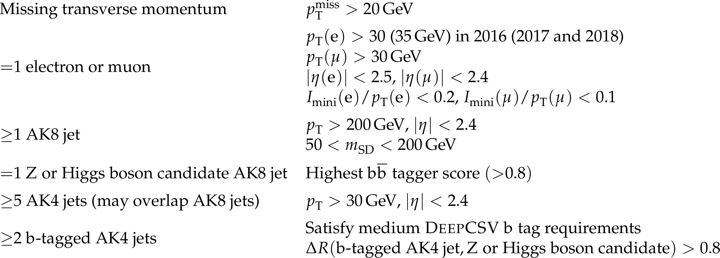
Summary of the reconstructed object and event selection requirements. |

png pdf |
Table 3:
The observed and expected best fit ($ \pm $1 standard deviation) signal strength modifiers $\mu _{{{\mathrm{t} \mathrm{\bar{t}}} \mathrm{Z}}}$ and $\mu _{{{\mathrm{t} \mathrm{\bar{t}}} \mathrm{H}}}$ for simulated $ {p_{\mathrm {T}}} ^{\mathrm{Z}}$ or $ {p_{\mathrm {T}}} ^{\mathrm{H}} > $ 200 GeV. The observed uncertainties are broken down into the components arising from the limited size of the data, the limited size of the simulation samples, experimental uncertainties, and theoretical uncertainties. |
png pdf |
Table 4:
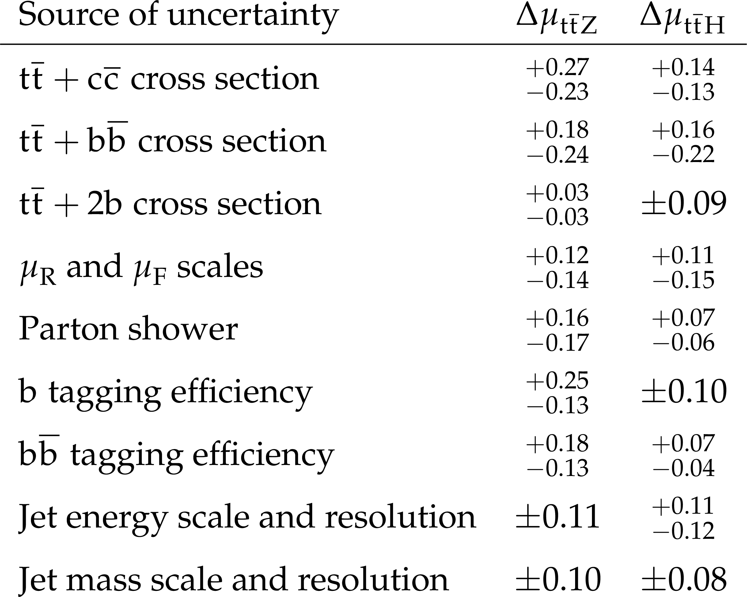
The magnitudes of the major sources of systematic uncertainty in the measurement of the signal strength modifiers $\mu _{{{\mathrm{t} \mathrm{\bar{t}}} \mathrm{Z}}}$ and $\mu _{{{\mathrm{t} \mathrm{\bar{t}}} \mathrm{H}}}$ for simulated $ {p_{\mathrm {T}}} ^{\mathrm{Z}}$ or $ {p_{\mathrm {T}}} ^{\mathrm{H}} > $ 200 GeV. |
png pdf |
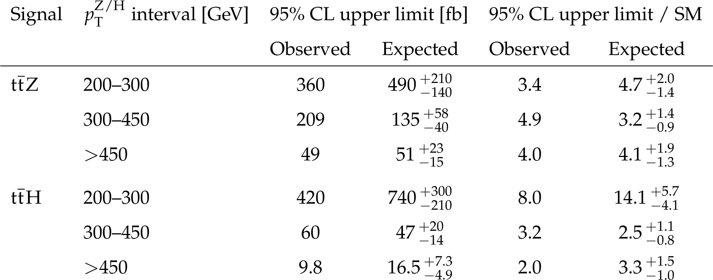
Table 5:
Observed and median expected 95% CL upper limits on the $\mathrm{t\bar{t}}$Z and $\mathrm{t\bar{t}}$H differential cross sections and on their ratios to the SM predictions for three $ {p_{\mathrm {T}}} ^{\mathrm{Z} /\mathrm{H}}$ intervals. The range given with the median expected 95% CL upper limits indicates the range in which 68% of the upper limits are expected to fall, assuming the SM hypothesis. |
png pdf |
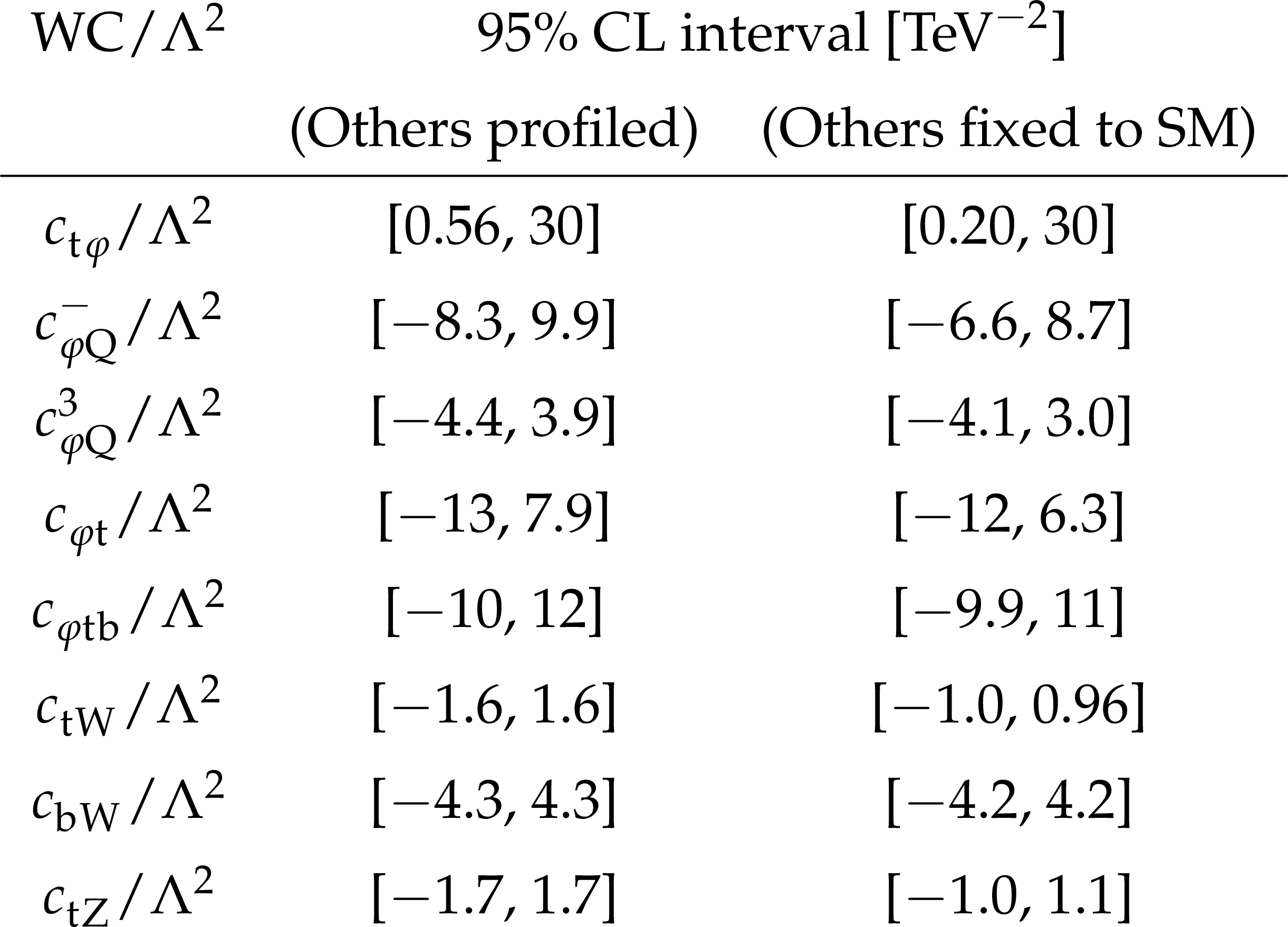
Table 6:
Observed 95% CL intervals for the eight WCs in the EFT model. The intervals are determined by scanning over a single WC while either profiling the other seven WCs or fixing them to their SM value of zero. |
png pdf |
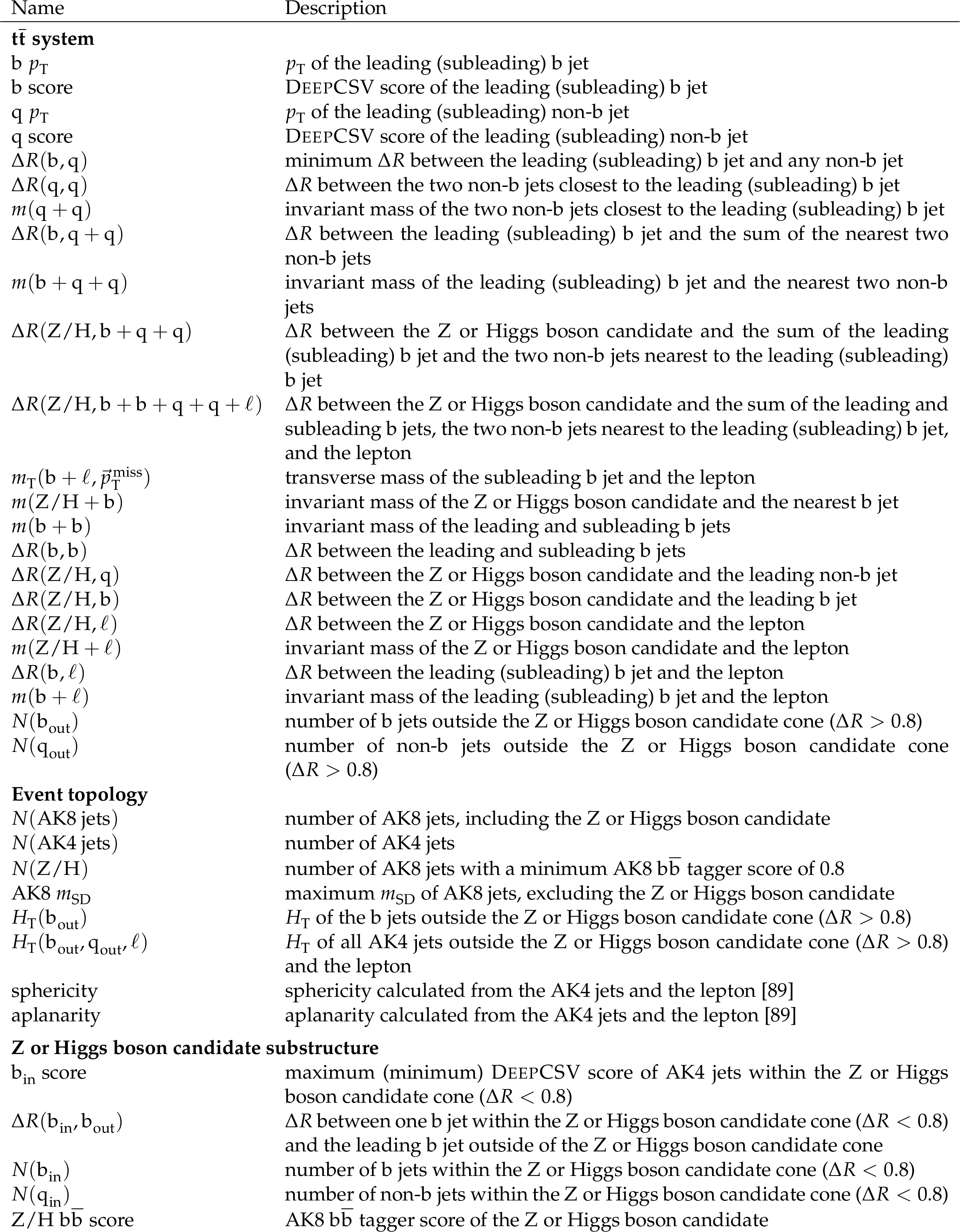
Table A1:
Comprehensive list of the input variables of the DNN, which is described in Section 6. The "+'' represents the relativistic four-momentum sum. Some variables are calculated for both the highest ${p_{\mathrm {T}}}$ (leading) and second-highest ${p_{\mathrm {T}}}$ (subleading) jet as indicated. |
| Summary |
|
Measurements of the signal strengths and 95% confidence level upper limits on the differential cross sections for production of $\mathrm{t\bar{t}}$Z and $\mathrm{t\bar{t}}$H events, where H refers to the Higgs boson, are presented along with constraints on the Wilson coefficients of a leading-order effective field theory. The analysis is performed using the $\mathrm{b\bar{b}}$ decay mode of the Z or Higgs boson and the lepton plus jets channel of the associated $\mathrm{t\bar{t}}$ pair. The Z or Higgs boson is required to be Lorentz boosted, with transverse momentum ${p_{\mathrm{T}}} > $ 200 GeV. A deep neural network is employed to discriminate between the $\mathrm{t\bar{t}}$Z and $\mathrm{t\bar{t}}$H signal events and the background, which is dominated by $\mathrm{t\bar{t}}{+}$jets production. The data correspond to an integrated luminosity of 138 fb$^{-1}$ collected with the CMS detector at the CERN LHC from 2016 through 2018. The data are binned as a function of the deep neural network score and the reconstructed ${p_{\mathrm{T}}}$ and mass of the Z or Higgs boson. Binned maximum likelihood fits are employed to extract the observables from the data. The data are found to be consistent with the expectations from the standard model. The signal strength modifiers for boosted $\mathrm{t\bar{t}}$Z and $\mathrm{t\bar{t}}$H production are measured to be $\mu_{{\mathrm{t\bar{t}}\mathrm{Z}} } = $ 0.65$^{+1.04}_{-0.98}$ and $\mu_{{\mathrm{t\bar{t}}\mathrm{H}} } =$ -0.27$^{+0.86}_{-0.83}$, which are both consistent with the expected value, 1. The 95% confidence level upper limits on the differential $\mathrm{t\bar{t}}$Z and $\mathrm{t\bar{t}}$H cross sections range from 2 to 5 times the standard model predicted cross sections for Z or Higgs boson ${p_{\mathrm{T}}} > $ 300 GeV. Results are also presented on eight parameters of a leading-order effective field theory that have a large impact on boosted $\mathrm{t\bar{t}}$Z and $\mathrm{t\bar{t}}$H production. These results represent the most restrictive limits to date on the cross sections for the production of $\mathrm{t\bar{t}}$Z and $\mathrm{t\bar{t}}$H with Z or Higgs boson ${p_{\mathrm{T}}} > $ 450 GeV. The limits on the Wilson coefficients in the effective field theory are consistent and, in some cases, competitive with the best previous limits. |
| References | ||||
| 1 | V. C. Rubin and W. K. Ford, Jr. | Rotation of the Andromeda nebula from a spectroscopic survey of emission regions | Astrophys. J. 159 (1970) 379 | |
| 2 | Planck Collaboration | Planck 2018 results. VI. cosmological parameters | Astron. Astrophys. 641 (2020) A6 | 1807.06209 |
| 3 | D. Clowe, A. Gonzalez, and M. Markevitch | Weak lensing mass reconstruction of the interacting cluster 1E 0657-558: Direct evidence for the existence of dark matter | Astrophys. J. 604 (2004) 596 | astro-ph/0312273 |
| 4 | R. K. Kaul and P. Majumdar | Cancellation of quadratically divergent mass corrections in globally supersymmetric spontaneously broken gauge theories | NPB 199 (1982) 36 | |
| 5 | R. Barbieri and G. F. Giudice | Upper bounds on supersymmetric particle masses | NPB 306 (1988) 63 | |
| 6 | W. Buchmuller and D. Wyler | Effective Lagrangian analysis of new interactions and flavor conservation | NPB 268 (1986) 621 | |
| 7 | B. Grzadkowski, M. Iskrzyński, M. Misiak, and J. Rosiek | Dimension-six terms in the standard model Lagrangian | JHEP 10 (2010) 085 | 1008.4884 |
| 8 | A. Falkowski and R. Rattazzi | Which EFT | JHEP 10 (2019) 255 | 1902.05936 |
| 9 | C. Degrande et al. | Effective field theory: A modern approach to anomalous couplings | Annals Phys. 335 (2013) 21 | 1205.4231 |
| 10 | A. Kobach | Baryon number, lepton number, and operator dimension in the standard model | PLB 758 (2016) 455 | 1604.05726 |
| 11 | Particle Data Group, P. A. Zyla et al. | Review of particle physics | Prog. Theor. Exp. Phys. 2020 (2020) 083C01 | |
| 12 | J. A. Aguilar-Saavedra et al. | Interpreting top-quark LHC measurements in the standard-model effective field theory | LHC TOP WG note CERN-LPCC-2018-01 | 1802.07237 |
| 13 | ATLAS Collaboration | Measurement of the $ \mathrm{t\bar{t}}$Z and $ \mathrm{t\bar{t}}$W cross sections in proton-proton collisions at $ \sqrt{s}= $ 13 TeV with the ATLAS detector | PRD 99 (2019) 072009 | 1901.03584 |
| 14 | ATLAS Collaboration | Measurements of the inclusive and differential production cross sections of a top-quark-antiquark pair in association with a Z boson at $ \sqrt{s}= $ 13 TeV with the ATLAS detector | EPJC 81 (2021) 737 | 2103.12603 |
| 15 | CMS Collaboration | Measurement of the cross section for top quark pair production in association with a W or Z boson in proton-proton collisions at $ \sqrt{s}= $ 13 TeV | JHEP 08 (2018) 011 | CMS-TOP-17-005 1711.02547 |
| 16 | CMS Collaboration | Measurement of top quark pair production in association with a Z boson in proton-proton collisions at $ \sqrt{s}= $ 13 TeV | JHEP 03 (2020) 056 | CMS-TOP-18-009 1907.11270 |
| 17 | ATLAS Collaboration | Observation of Higgs boson production in association with a top quark pair at the LHC with the ATLAS detector | PLB 784 (2018) 173 | 1806.00425 |
| 18 | ATLAS Collaboration | $ CP $ properties of Higgs boson interactions with top quarks in the $ \mathrm{t\bar{t}}$H and tH processes using H $ \rightarrow \gamma\gamma $ with the ATLAS detector | PRL 125 (2020) 061802 | 2004.04545 |
| 19 | ATLAS Collaboration | Measurement of Higgs boson decay into b-quarks in associated production with a top-quark pair in pp collisions at $ \sqrt{s}= $ 13 TeV with the ATLAS detector | JHEP 06 (2022) 097 | 2111.06712 |
| 20 | CMS Collaboration | Observation of $ \mathrm{t\bar{t}}$H production | PRL 120 (2018) 231801 | CMS-HIG-17-035 1804.02610 |
| 21 | CMS Collaboration | Search for $ \mathrm{t\bar{t}}$H production in the all-jet final state in proton-proton collisions at $ \sqrt{s}= $ 13 TeV | JHEP 06 (2018) 101 | CMS-HIG-17-022 1803.06986 |
| 22 | CMS Collaboration | Search for $ \mathrm{t\bar{t}}$H production in the H $\to\mathrm{b\bar{b}} $ decay channel with leptonic $ \mathrm{t\bar{t}} $ decays in proton-proton collisions at $ \sqrt{s}= $ 13 TeV | JHEP 03 (2019) 026 | CMS-HIG-17-026 1804.03682 |
| 23 | CMS Collaboration | Measurements of $ \mathrm{t\bar{t}}$H production and the $ CP $ structure of the Yukawa interaction between the Higgs boson and top quark in the diphoton decay channel | PRL 125 (2020) 061801 | CMS-HIG-19-013 2003.10866 |
| 24 | CMS Collaboration | Measurement of the Higgs boson production rate in association with top quarks in final states with electrons, muons, and hadronically decaying tau leptons at $ \sqrt{s}= $ 13 TeV | EPJC 81 (2021) 378 | CMS-HIG-19-008 2011.03652 |
| 25 | CMS Collaboration | Search for new physics in top quark production with additional leptons in proton-proton collisions at $ \sqrt{s}= $ 13 TeV using effective field theory | JHEP 03 (2021) 095 | CMS-TOP-19-001 2012.04120 |
| 26 | CMS Collaboration | Measurement of the inclusive and differential $ \mathrm{t\bar{t}}\gamma $ cross sections in the single-lepton channel and EFT interpretation at $ \sqrt{s}= $ 13 TeV | JHEP 12 (2021) 180 | CMS-TOP-18-010 2107.01508 |
| 27 | CMS Collaboration | Probing effective field theory operators in the associated production of top quarks with a Z boson in multilepton final states at $ \sqrt{s}= $ 13 TeV | JHEP 12 (2021) 083 | CMS-TOP-21-001 2107.13896 |
| 28 | CMS Collaboration | Measurement of the inclusive and differential $ \mathrm{t\bar{t}}\gamma $ cross sections in the dilepton channel and effective field theory interpretation in proton-proton collisions at $ \sqrt{s}= $ 13 TeV | JHEP 05 (2022) 091 | CMS-TOP-21-004 2201.07301 |
| 29 | CMS Collaboration | HEPData record for this analysis | link | |
| 30 | CMS Collaboration | Performance of the CMS Level-1 trigger in proton-proton collisions at $ \sqrt{s}= $ 13 TeV | JINST 15 (2020) P10017 | CMS-TRG-17-001 2006.10165 |
| 31 | CMS Collaboration | The CMS trigger system | JINST 12 (2017) P01020 | CMS-TRG-12-001 1609.02366 |
| 32 | CMS Collaboration | The CMS experiment at the CERN LHC | JINST 3 (2008) S08004 | CMS-00-001 |
| 33 | CMS Collaboration | Precision luminosity measurement in proton-proton collisions at $ \sqrt{s}= $ 13 TeV in 2015 and 2016 at CMS | EPJC 81 (2021) 800 | CMS-LUM-17-003 2104.01927 |
| 34 | CMS Collaboration | CMS luminosity measurement for the 2017 data-taking period at $ \sqrt{s}= $ 13 TeV | CMS-PAS-LUM-17-004 | CMS-PAS-LUM-17-004 |
| 35 | CMS Collaboration | CMS luminosity measurement for the 2018 data-taking period at $ \sqrt{s}= $ 13 TeV | CMS-PAS-LUM-18-002 | CMS-PAS-LUM-18-002 |
| 36 | J. Alwall et al. | The automated computation of tree-level and next-to-leading order differential cross sections, and their matching to parton shower simulations | JHEP 07 (2014) 079 | 1405.0301 |
| 37 | P. Nason | A new method for combining NLO QCD with shower Monte Carlo algorithms | JHEP 11 (2004) 040 | hep-ph/0409146 |
| 38 | S. Frixione, P. Nason, and C. Oleari | Matching NLO QCD computations with parton shower simulations: the POWHEG method | JHEP 11 (2007) 070 | 0709.2092 |
| 39 | S. Alioli, P. Nason, C. Oleari, and E. Re | A general framework for implementing NLO calculations in shower Monte Carlo programs: the POWHEG BOX | JHEP 06 (2010) 043 | 1002.2581 |
| 40 | H. B. Hartanto, B. Jager, L. Reina, and D. Wackeroth | Higgs boson production in association with top quarks in the POWHEG BOX | PRD 91 (2015) 094003 | 1501.04498 |
| 41 | A. Kulesza et al. | Associated production of a top quark pair with a heavy electroweak gauge boson at NLO+NNLL accuracy | EPJC 79 (2019) 249 | 1812.08622 |
| 42 | LHC Higgs Cross Section Working Group | Handbook of LHC Higgs cross sections: 4. Deciphering the nature of the Higgs sector | CERN-2017-002-M | 1610.07922 |
| 43 | T. Ježo, J. M. Lindert, N. Moretti, and S. Pozzorini | New NLOPS predictions for $ \mathrm{t\bar{t}}+\mathrm{b} $-jet production at the LHC | EPJC 78 (2018) 502 | 1802.00426 |
| 44 | F. Buccioni, S. Kallweit, S. Pozzorini, and M. F. Zoller | NLO QCD predictions for $ \mathrm{t\bar{t}}\mathrm{b\bar{b}} $ production in association with a light jet at the LHC | JHEP 12 (2019) 015 | 1907.13624 |
| 45 | S. Frixione, P. Nason, and G. Ridolfi | A positive-weight next-to-leading-order Monte Carlo for heavy flavour hadroproduction | JHEP 09 (2007) 126 | 0707.3088 |
| 46 | M. Czakon et al. | Top-pair production at the LHC through NNLO QCD and NLO EW | JHEP 10 (2017) 186 | 1705.04105 |
| 47 | M. Beneke, P. Falgari, S. Klein, and C. Schwinn | Hadronic top-quark pair production with NNLL threshold resummation | NPB 855 (2012) 695 | 1109.1536 |
| 48 | M. Cacciari et al. | Top-pair production at hadron colliders with next-to-next-to-leading logarithmic soft-gluon resummation | PLB 710 (2012) 612 | 1111.5869 |
| 49 | P. Barnreuther, M. Czakon, and A. Mitov | Percent-level-precision physics at the Tevatron: next-to-next-to-leading order QCD corrections to $ \mathrm{q\bar{q}} \to \mathrm{t\bar{t}}$ + X | PRL 109 (2012) 132001 | 1204.5201 |
| 50 | M. Czakon and A. Mitov | NNLO corrections to top-pair production at hadron colliders: the all-fermionic scattering channels | JHEP 12 (2012) 054 | 1207.0236 |
| 51 | M. Czakon and A. Mitov | NNLO corrections to top pair production at hadron colliders: the quark-gluon reaction | JHEP 01 (2013) 080 | 1210.6832 |
| 52 | M. Czakon, P. Fiedler, and A. Mitov | Total top-quark pair-production cross section at hadron colliders through $ O({\alpha_S}^4) $ | PRL 110 (2013) 252004 | 1303.6254 |
| 53 | M. Czakon and A. Mitov | Top++: a program for the calculation of the top-pair cross-section at hadron colliders | CPC 185 (2014) 2930 | 1112.5675 |
| 54 | S. Alioli, P. Nason, C. Oleari, and E. Re | NLO single-top production matched with shower in POWHEG: $ s $- and $ t $-channel contributions | JHEP 09 (2009) 111 | 0907.4076 |
| 55 | E. Re | Single-top Wt-channel production matched with parton showers using the POWHEG method | EPJC 71 (2011) 1547 | 1009.2450 |
| 56 | S. Quackenbush, R. Gavin, Y. Li, and F. Petriello | W physics at the LHC with FEWZ 2.1 | CPC 184 (2013) 209 | 1201.5896 |
| 57 | Y. Li and F. Petriello | Combining QCD and electroweak corrections to dilepton production in the framework of the FEWZ simulation code | PRD 86 (2012) 094034 | 1208.5967 |
| 58 | N. Kidonakis | Two-loop soft anomalous dimensions for single top quark associated production with a W$ ^{-}$ or H$ ^{-}$ | PRD 82 (2010) 054018 | 1005.4451 |
| 59 | M. Aliev et al. | HATHOR: hadronic top and heavy quarks cross section calculator | CPC 182 (2011) 1034 | 1007.1327 |
| 60 | P. Kant et al. | HatHor for single top-quark production: updated predictions and uncertainty estimates for single top-quark production in hadronic collisions | CPC 191 (2015) 74 | 1406.4403 |
| 61 | R. Frederix and S. Frixione | Merging meets matching in MC@NLO | JHEP 12 (2012) 061 | 1209.6215 |
| 62 | M. L. Mangano, M. Moretti, F. Piccinini, and M. Treccani | Matching matrix elements and shower evolution for top-pair production in hadronic collisions | JHEP 01 (2007) 013 | hep-ph/0611129 |
| 63 | CMS Collaboration | Extraction and validation of a new set of CMS PYTHIA8 tunes from underlying-event measurements | EPJC 80 (2020) 4 | CMS-GEN-17-001 1903.12179 |
| 64 | CMS Collaboration | Event generator tunes obtained from underlying event and multiparton scattering measurements | EPJC 76 (2016) 155 | CMS-GEN-14-001 1512.00815 |
| 65 | NNPDF Collaboration | Parton distributions from high-precision collider data | EPJC 77 (2017) 663 | 1706.00428 |
| 66 | NNPDF Collaboration | Parton distributions for the LHC run II | JHEP 04 (2015) 040 | 1410.8849 |
| 67 | GEANT4 Collaboration | GEANT4--a simulation toolkit | NIMA 506 (2003) 250 | |
| 68 | R. Goldouzian et al. | Matching in pp $ \to \mathrm{t\bar{t}} \mathrm{W}/\mathrm{Z}/\mathrm{h} $ + jet SMEFT studies | JHEP 06 (2021) 151 | 2012.06872 |
| 69 | C. Degrande et al. | Automated one-loop computations in the standard model effective field theory | PRD 103 (2021) 096024 | 2008.11743 |
| 70 | CMS Collaboration | Particle-flow reconstruction and global event description with the CMS detector | JINST 12 (2017) P10003 | CMS-PRF-14-001 1706.04965 |
| 71 | CMS Collaboration | Performance of missing transverse momentum reconstruction in proton-proton collisions at $ \sqrt{s}= $ 13 TeV using the CMS detector | JINST 14 (2019) P07004 | CMS-JME-17-001 1903.06078 |
| 72 | CMS Collaboration | Technical proposal for the Phase-II upgrade of the Compact Muon Solenoid | CMS-PAS-TDR-15-002 | CMS-PAS-TDR-15-002 |
| 73 | CMS Collaboration | Performance of electron reconstruction and selection with the CMS detector in proton-proton collisions at $ \sqrt{s}= $ 8 TeV | JINST 10 (2015) P06005 | CMS-EGM-13-001 1502.02701 |
| 74 | CMS Collaboration | Performance of the CMS muon detector and muon reconstruction with proton-proton collisions at $ \sqrt{s}= $ 13 TeV | JINST 13 (2018) P06015 | CMS-MUO-16-001 1804.04528 |
| 75 | CMS Collaboration | Search for supersymmetry in pp collisions at $ \sqrt{s}= $ 13 TeV in the single-lepton final state using the sum of masses of large-radius jets | JHEP 08 (2016) 122 | CMS-SUS-15-007 1605.04608 |
| 76 | M. Cacciari, G. P. Salam, and G. Soyez | The anti-$ {k_{\mathrm{T}}} $ jet clustering algorithm | JHEP 04 (2008) 063 | 0802.1189 |
| 77 | M. Cacciari, G. P. Salam, and G. Soyez | FastJet user manual | EPJC 72 (2012) 1896 | 1111.6097 |
| 78 | CMS Collaboration | Pileup mitigation at CMS in 13 TeV data | JINST 15 (2020) P09018 | CMS-JME-18-001 2003.00503 |
| 79 | D. Bertolini, P. Harris, M. Low, and N. Tran | Pileup per particle identification | JHEP 10 (2014) 059 | 1407.6013 |
| 80 | M. Dasgupta, A. Fregoso, S. Marzani, and G. P. Salam | Towards an understanding of jet substructure | JHEP 09 (2013) 029 | 1307.0007 |
| 81 | A. J. Larkoski, S. Marzani, G. Soyez, and J. Thaler | Soft drop | JHEP 05 (2014) 146 | 1402.2657 |
| 82 | CMS Collaboration | Identification of heavy, energetic, hadronically decaying particles using machine-learning techniques | JINST 15 (2020) P06005 | CMS-JME-18-002 2004.08262 |
| 83 | M. Cacciari and G. P. Salam | Pileup subtraction using jet areas | PLB 659 (2008) 119 | 0707.1378 |
| 84 | CMS Collaboration | Jet energy scale and resolution in the CMS experiment in pp collisions at 8 TeV | JINST 12 (2017) P02014 | CMS-JME-13-004 1607.03663 |
| 85 | CMS Collaboration | Identification of heavy-flavour jets with the CMS detector in pp collisions at 13 TeV | JINST 13 (2018) P05011 | CMS-BTV-16-002 1712.07158 |
| 86 | J. G. Kreer | A question of terminology | IRE Trans. Inf. Theory 3 (1957) 208 | |
| 87 | C. E. Shannon | A mathematical theory of communication | Bell Syst. Tech. J. 27 (1948) 379 | |
| 88 | ATLAS Collaboration | Measurement of event shapes at large momentum transfer with the ATLAS detector in pp collisions at $ \sqrt{s}= $ 7 TeV | EPJC 72 (2012) 2211 | 1206.2135 |
| 89 | S. Ioffe and C. Szegedy | Batch normalization: accelerating deep network training by reducing internal covariate shift | Proc. Mach. Learn. Res. 37 (2015) 448 | 1502.03167 |
| 90 | N. Srivastava et al. | Dropout: a simple way to prevent neural networks from overfitting | J. Mach. Learn. Res. 15 (2014) 1929 | |
| 91 | T.-Y. Lin et al. | Focal loss for dense object detection | IEEE Trans. Pattern Anal. Mach. Intell. 42 (2020) 318 | 1708.02002 |
| 92 | R. J. Barlow and C. Beeston | Fitting using finite Monte Carlo samples | CPC 77 (1993) 219 | |
| 93 | J. S. Conway | Incorporating nuisance parameters in likelihoods for multisource spectra | in PHYSTAT 2011 2011 | 1103.0354 |
| 94 | J. Butterworth et al. | PDF4LHC recommendations for LHC run II | JPG 43 (2016) 023001 | 1510.03865 |
| 95 | G. Ridolfi, M. Ubiali, and M. Zaro | A fragmentation-based study of heavy quark production | JHEP 01 (2020) 196 | 1911.01975 |
| 96 | CMS Collaboration | First measurement of the cross section for top quark pair production with additional charm jets using dileptonic final states in pp collisions at $ \sqrt{s}= $ 13 TeV | PLB 820 (2021) 136565 | CMS-TOP-20-003 2012.09225 |
| 97 | CMS Collaboration | Measurement of the inelastic proton-proton cross section at $ \sqrt{s}= $ 13 TeV | JHEP 07 (2018) 161 | CMS-FSQ-15-005 1802.02613 |
| 98 | ATLAS and CMS Collaborations, and LHC Higgs Combination Group | Procedure for the LHC Higgs boson search combination in Summer 2011 | CMS-NOTE-2011-005 | |
| 99 | G. Cowan, K. Cranmer, E. Gross, and O. Vitells | Asymptotic formulae for likelihood-based tests of new physics | EPJC 71 (2011) 1554 | 1007.1727 |
| 100 | T. Junk | Confidence level computation for combining searches with small statistics | NIMA 434 (1999) 435 | hep-ex/9902006 |
| 101 | A. L. Read | Presentation of search results: The CLs technique | JPG 28 (2002) 2693 | |
| 102 | CMS Collaboration | Measurement and interpretation of differential cross sections for Higgs boson production at $ \sqrt{s}= $ 13 TeV | PLB 792 (2019) 369 | CMS-HIG-17-028 1812.06504 |
| 103 | CMS Collaboration | Measurement of the cross section for $ \mathrm{t\bar{t}} $ production with additional jets and b jets in pp collisions at $ \sqrt{s}= $ 13 TeV | JHEP 07 (2020) 125 | CMS-TOP-18-002 2003.06467 |
| 104 | CMS Collaboration | Measurement of the $ \mathrm{t\bar{t}}\mathrm{b\bar{b}} $ production cross section in the all-jet final state in pp collisions at $ \sqrt{s}= $ 13 TeV | PLB 803 (2020) 135285 | CMS-TOP-18-011 1909.05306 |
|
|
Compact Muon Solenoid LHC, CERN |
|

|

|

|

|

|