

Compact Muon Solenoid
LHC, CERN
| CMS-SMP-18-011 ; CERN-EP-2021-240 | ||
| Precision measurement of the W boson decay branching fractions in proton-proton collisions at $\sqrt{s} = $ 13 TeV | ||
| CMS Collaboration | ||
| 19 January 2022 | ||
| Phys. Rev. D 105 (2022) 072008 | ||
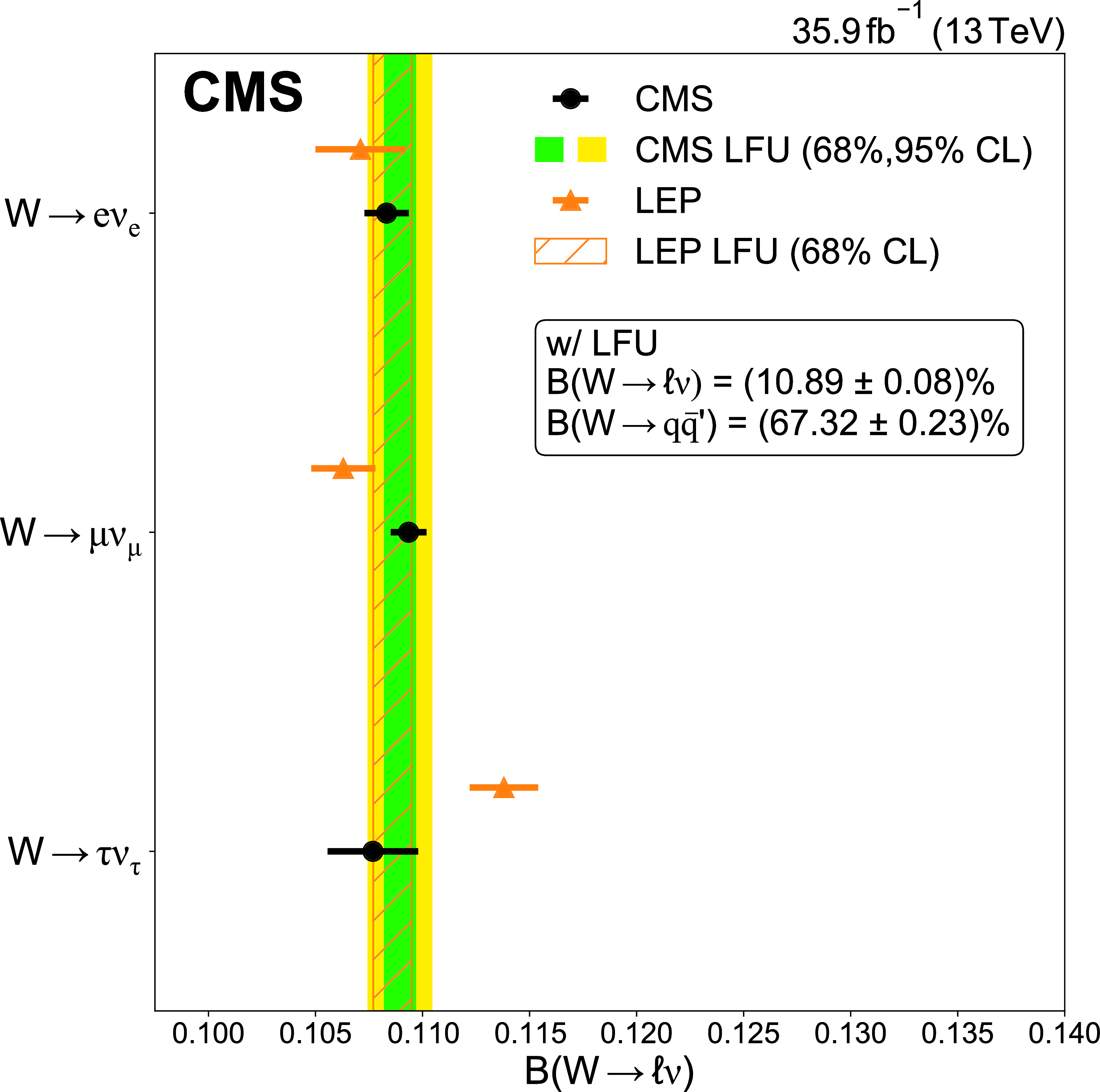
| Abstract: The leptonic and inclusive hadronic decay branching fractions of the W boson are measured using proton-proton collision data collected at $\sqrt{s} = $ 13 TeV by the CMS experiment at the CERN LHC, corresponding to an integrated luminosity of 35.9 fb$^{-1}$. Events characterized by the production of one or two W bosons are selected and categorized based on the multiplicity and flavor of reconstructed leptons, the number of jets, and the number of jets identified as originating from the hadronization of b quarks. A binned maximum likelihood estimate of the W boson branching fractions is performed simultaneously in each event category. The measured branching fractions of the W boson decaying into electron, muon, and tau lepton final states are (10.83 $\pm$ 0.10)%, (10.94 $\pm$ 0.08)%, and (10.77 $\pm$ 0.21)%, respectively, consistent with lepton flavor universality for the weak interaction. The average leptonic and inclusive hadronic decay branching fractions are estimated to be (10.89 $\pm$ 0.08)% and (67.32 $\pm$ 0.23)%, respectively. Based on the hadronic branching fraction, three standard model quantities are subsequently derived: the sum of squared elements in the first two rows of the Cabibbo-Kobayashi-Maskawa (CKM) matrix $\sum_{ij}|{V_{ij}} |^{2} = $ 1.984 $\pm$ 0.021, the CKM element $|{V_{\mathrm{c}\mathrm{s}}} | = $ 0.967 $\pm$ 0.011, and the strong coupling constant at the W boson mass scale, ${\alpha_S}(m^2_{\mathrm{W}}) = $ 0.095 $\pm$ 0.033. | ||
| Links: e-print arXiv:2201.07861 [hep-ex] (PDF) ; CDS record ; inSPIRE record ; HepData record ; CADI line (restricted) ; | ||
| Figures | |
png pdf |
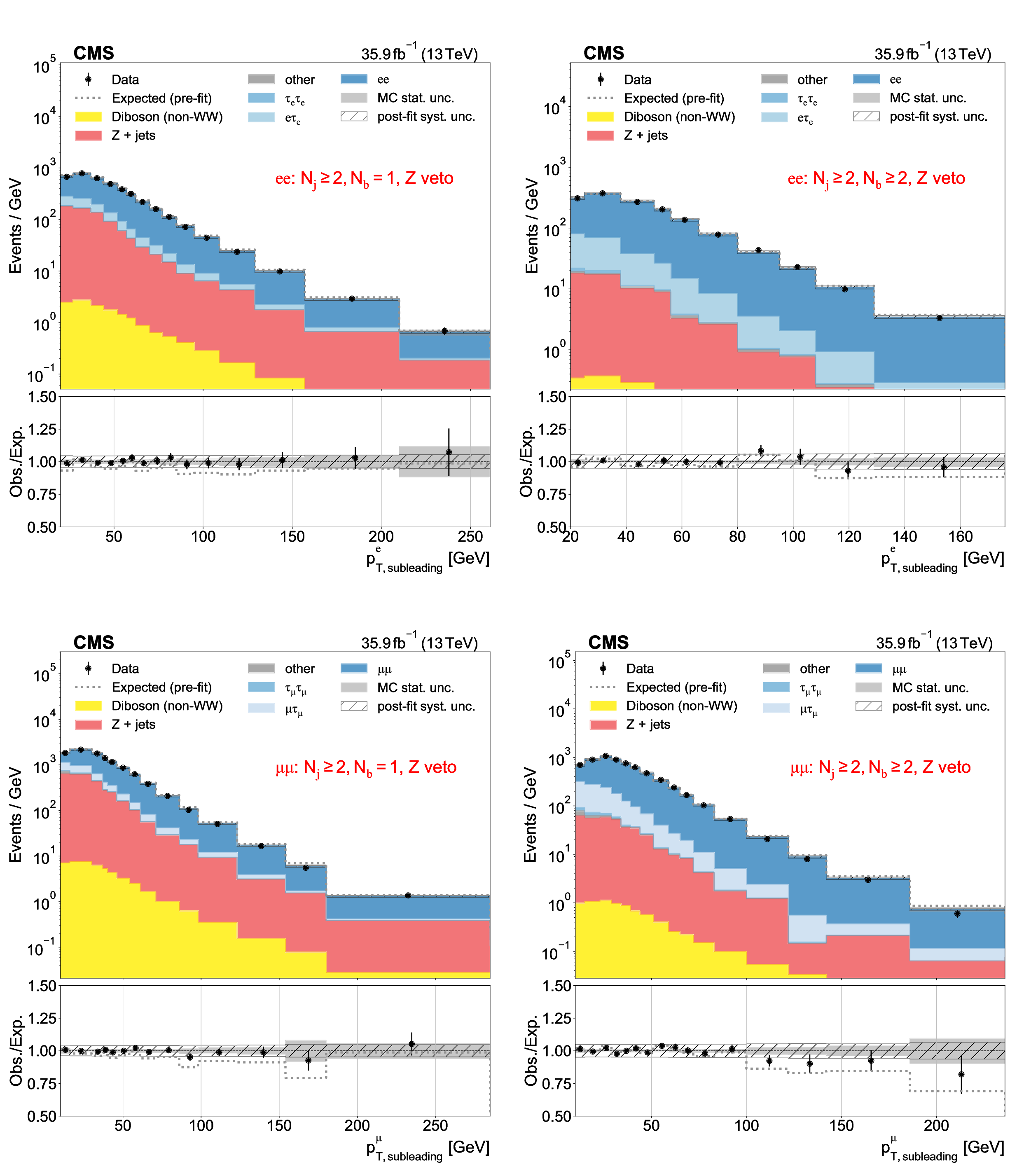
Figure 1:
Subleading electron and muon ${p_{\mathrm {T}}}$ distributions used as inputs for the binned likelihood fits for the $\mathrm{e} \mathrm{e} $ (upper) and $\mu \mu $ (lower) categories, respectively, with the requirement of one (left) or more than one (right) b-tagged jets. The lower subpanels show the ratio of data over pre-fit (dotted line) and post-fit (black circles) expectations, with associated MC statistical uncertainties (hatched area) and post-fit systematic uncertainties (shaded gray). Vertical bars on the data markers indicate statistical uncertainties. |

png pdf |
Figure 1-a:
Subleading electron and muon ${p_{\mathrm {T}}}$ distributions used as inputs for the binned likelihood fits for the $\mathrm{e} \mathrm{e} $ (upper) and $\mu \mu $ (lower) categories, respectively, with the requirement of one (left) or more than one (right) b-tagged jets. The lower subpanels show the ratio of data over pre-fit (dotted line) and post-fit (black circles) expectations, with associated MC statistical uncertainties (hatched area) and post-fit systematic uncertainties (shaded gray). Vertical bars on the data markers indicate statistical uncertainties. |
png pdf |
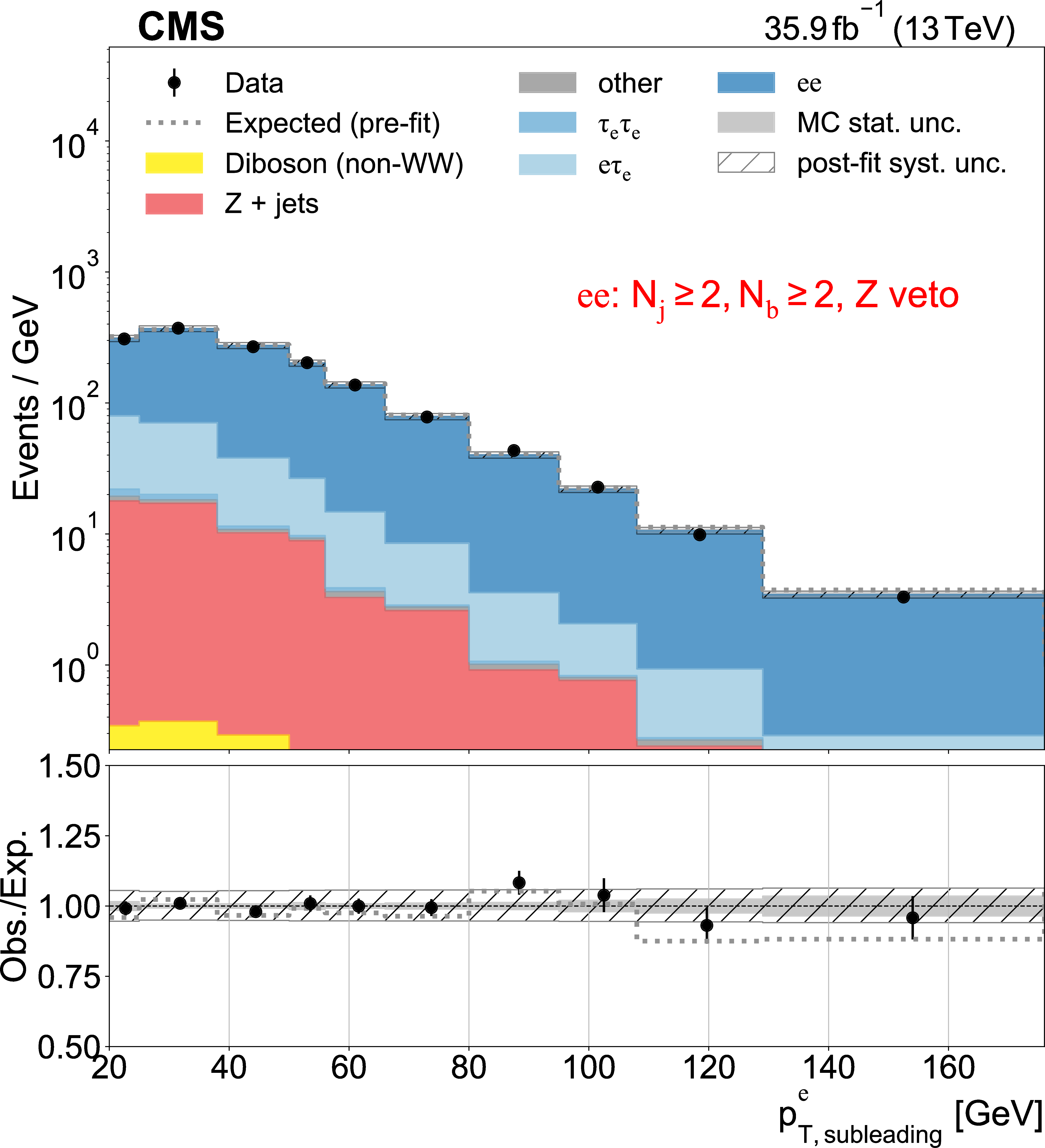
Figure 1-b:
Subleading electron and muon ${p_{\mathrm {T}}}$ distributions used as inputs for the binned likelihood fits for the $\mathrm{e} \mathrm{e} $ (upper) and $\mu \mu $ (lower) categories, respectively, with the requirement of one (left) or more than one (right) b-tagged jets. The lower subpanels show the ratio of data over pre-fit (dotted line) and post-fit (black circles) expectations, with associated MC statistical uncertainties (hatched area) and post-fit systematic uncertainties (shaded gray). Vertical bars on the data markers indicate statistical uncertainties. |
png pdf |
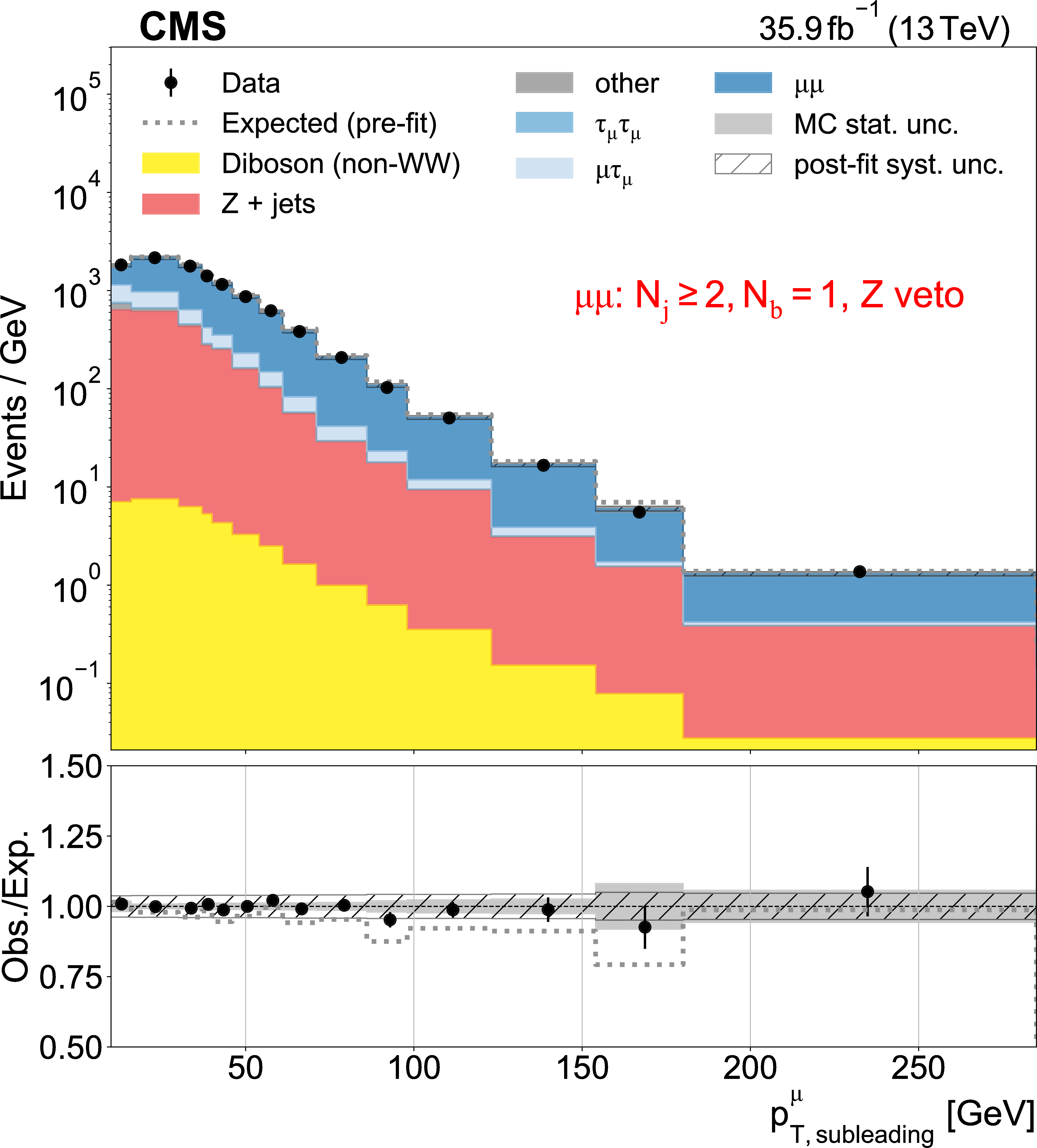
Figure 1-c:
Subleading electron and muon ${p_{\mathrm {T}}}$ distributions used as inputs for the binned likelihood fits for the $\mathrm{e} \mathrm{e} $ (upper) and $\mu \mu $ (lower) categories, respectively, with the requirement of one (left) or more than one (right) b-tagged jets. The lower subpanels show the ratio of data over pre-fit (dotted line) and post-fit (black circles) expectations, with associated MC statistical uncertainties (hatched area) and post-fit systematic uncertainties (shaded gray). Vertical bars on the data markers indicate statistical uncertainties. |
png pdf |
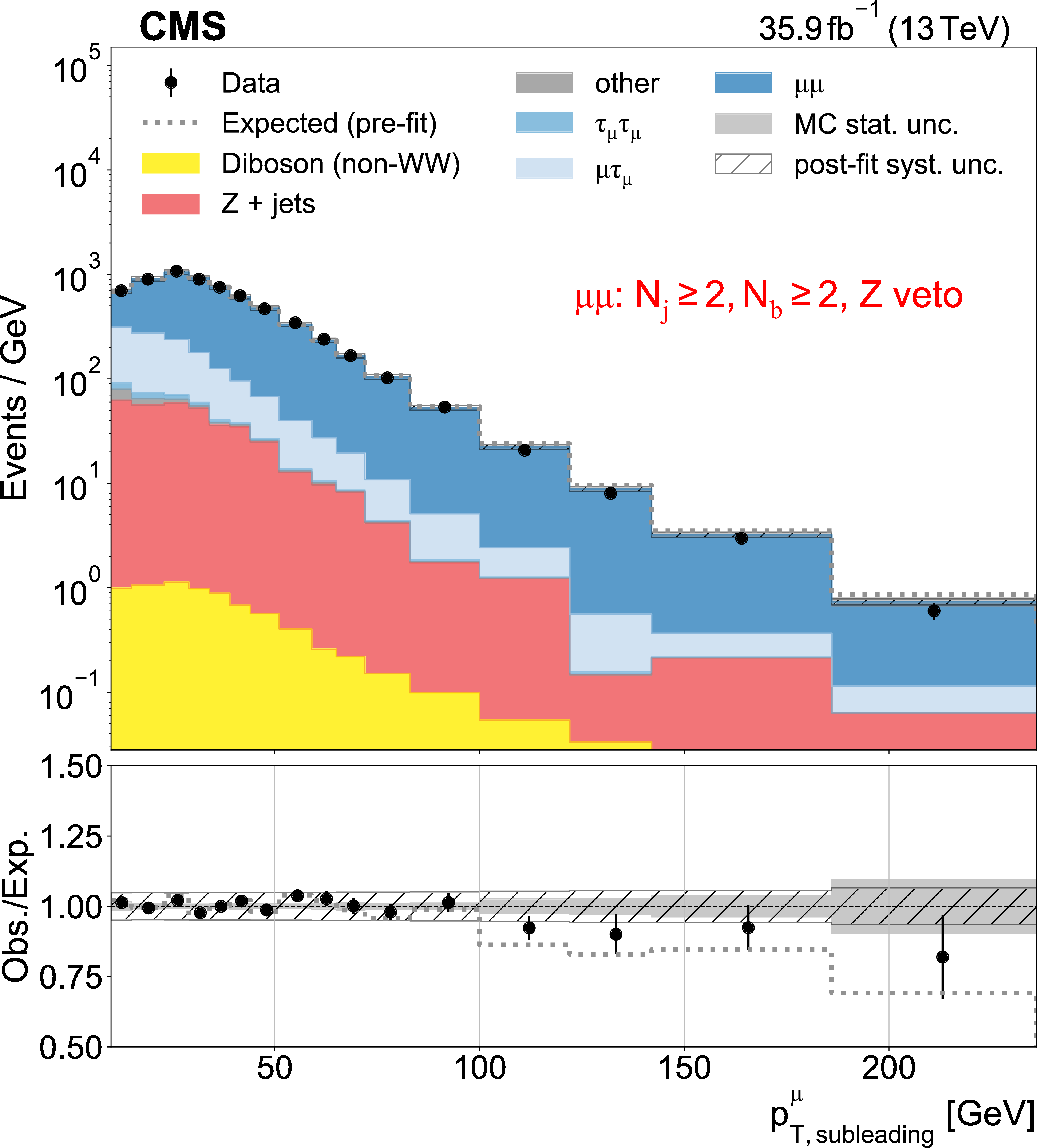
Figure 1-d:
Subleading electron and muon ${p_{\mathrm {T}}}$ distributions used as inputs for the binned likelihood fits for the $\mathrm{e} \mathrm{e} $ (upper) and $\mu \mu $ (lower) categories, respectively, with the requirement of one (left) or more than one (right) b-tagged jets. The lower subpanels show the ratio of data over pre-fit (dotted line) and post-fit (black circles) expectations, with associated MC statistical uncertainties (hatched area) and post-fit systematic uncertainties (shaded gray). Vertical bars on the data markers indicate statistical uncertainties. |
png pdf |
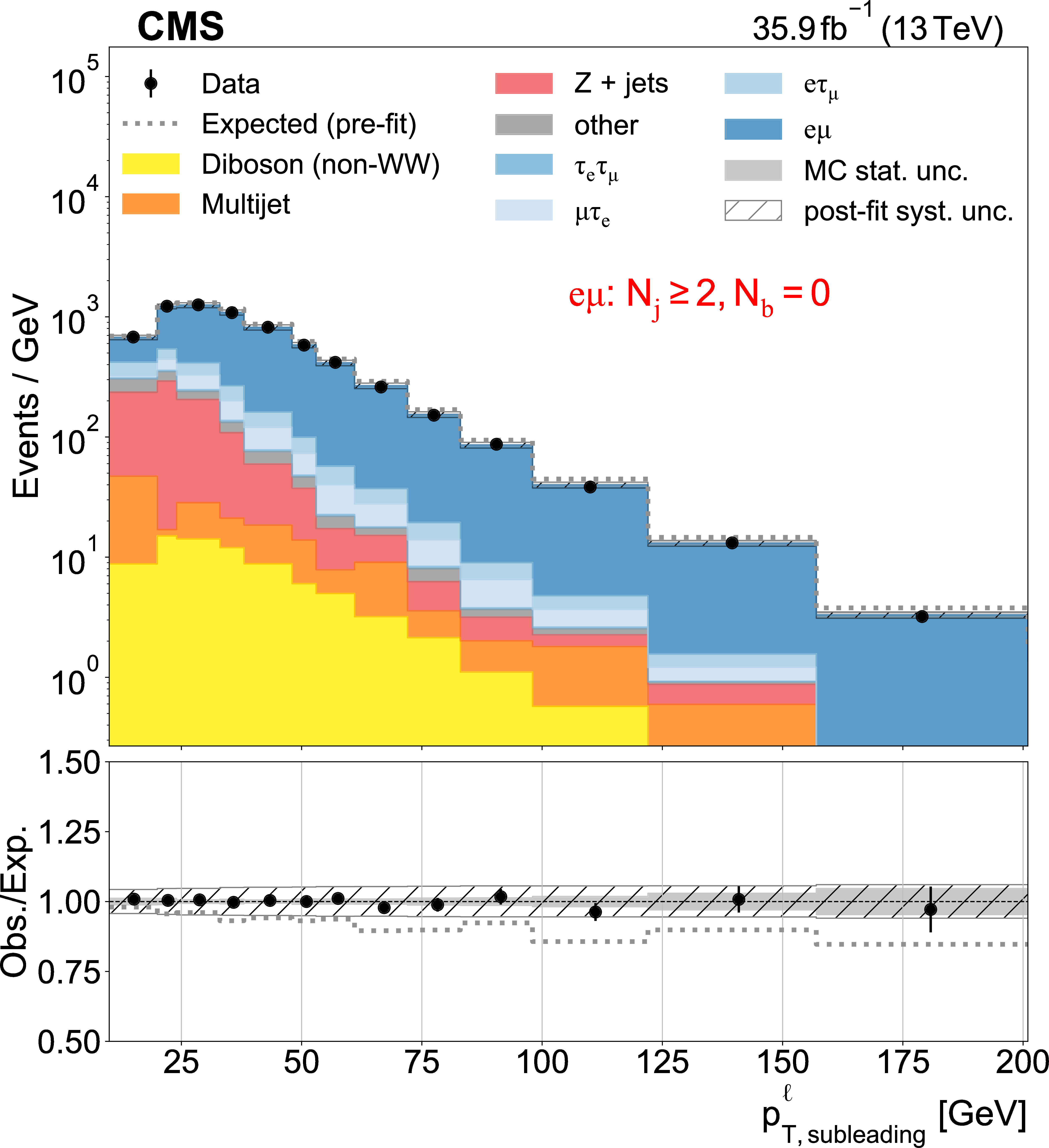
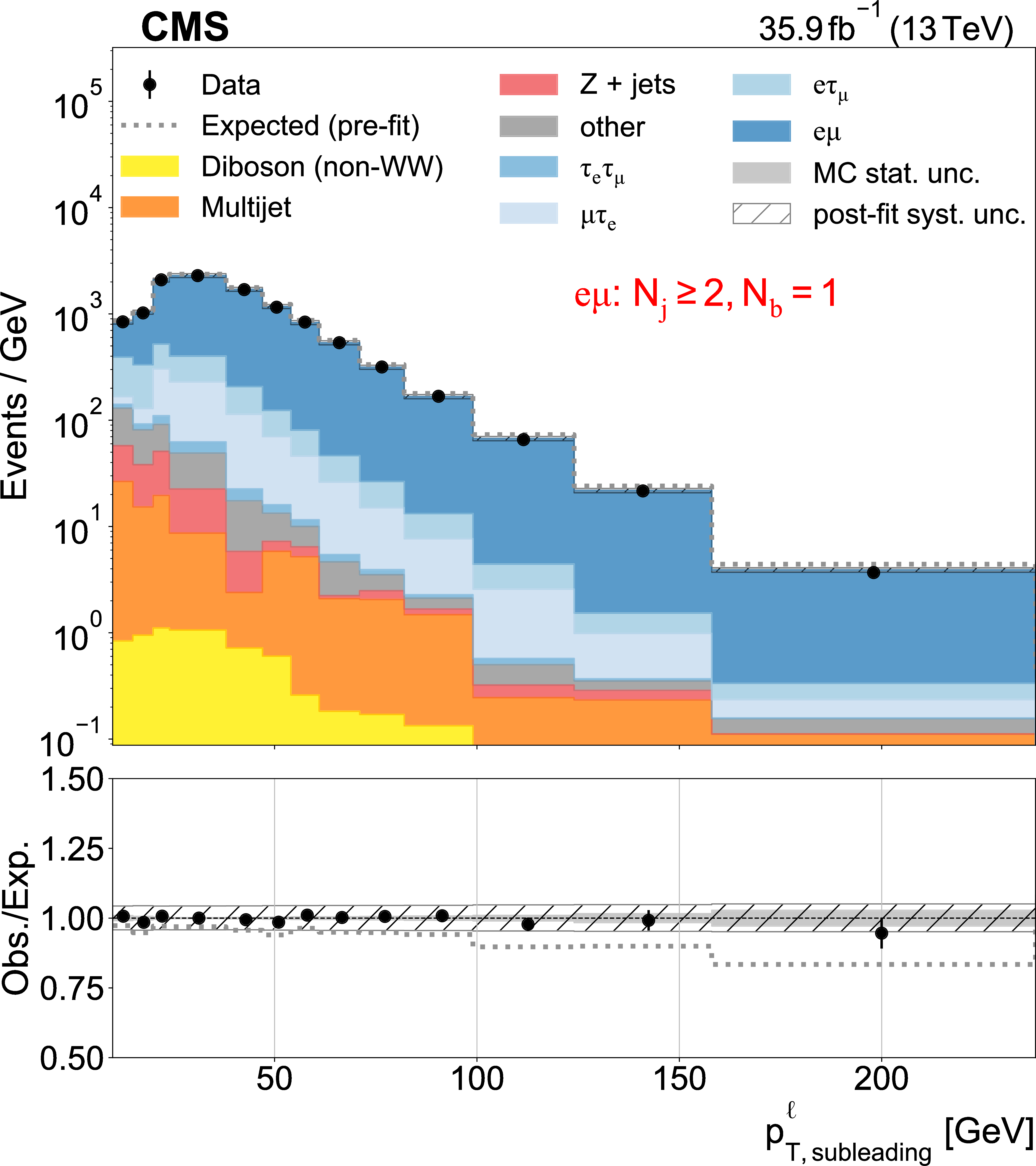
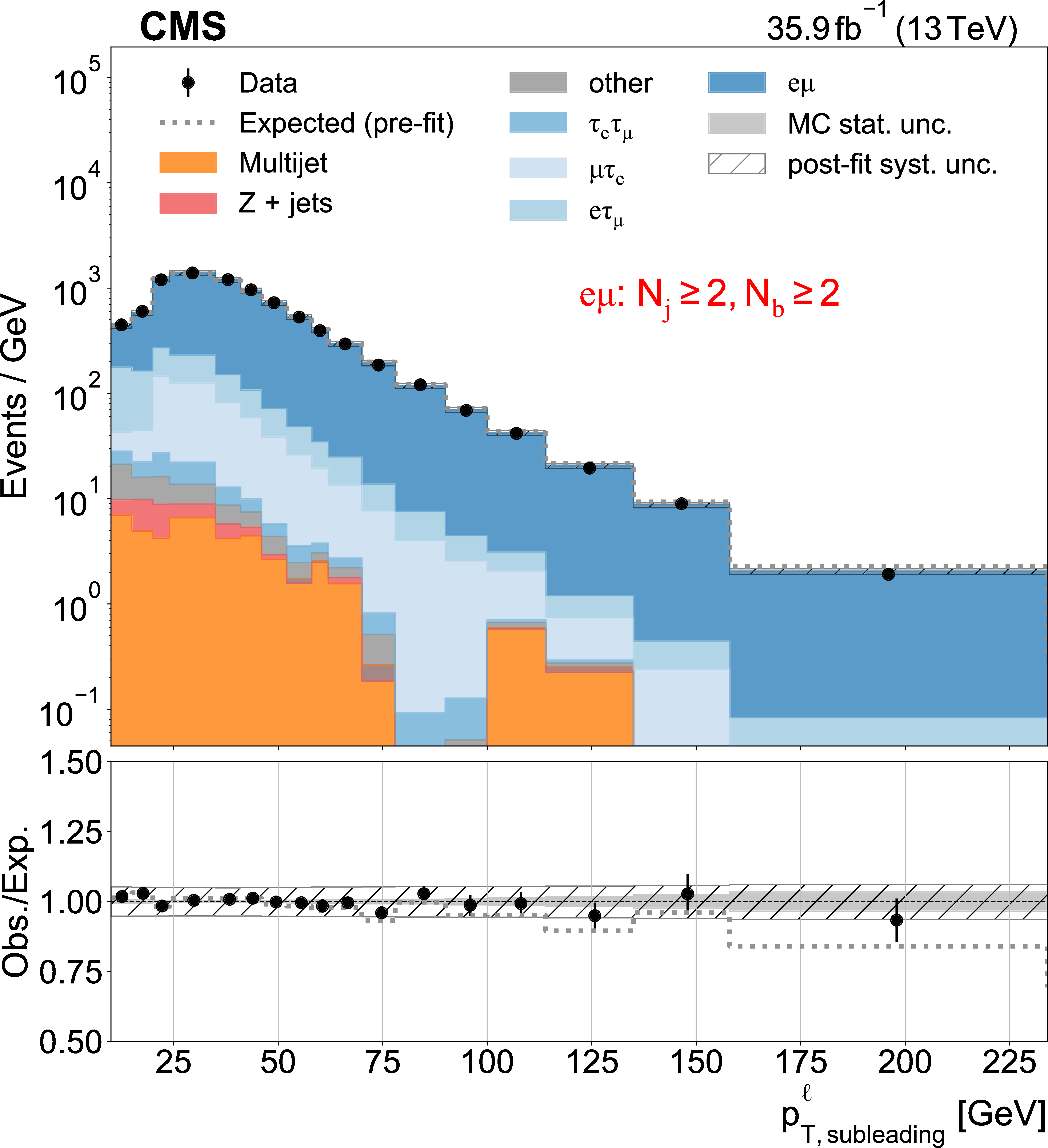
Figure 2:
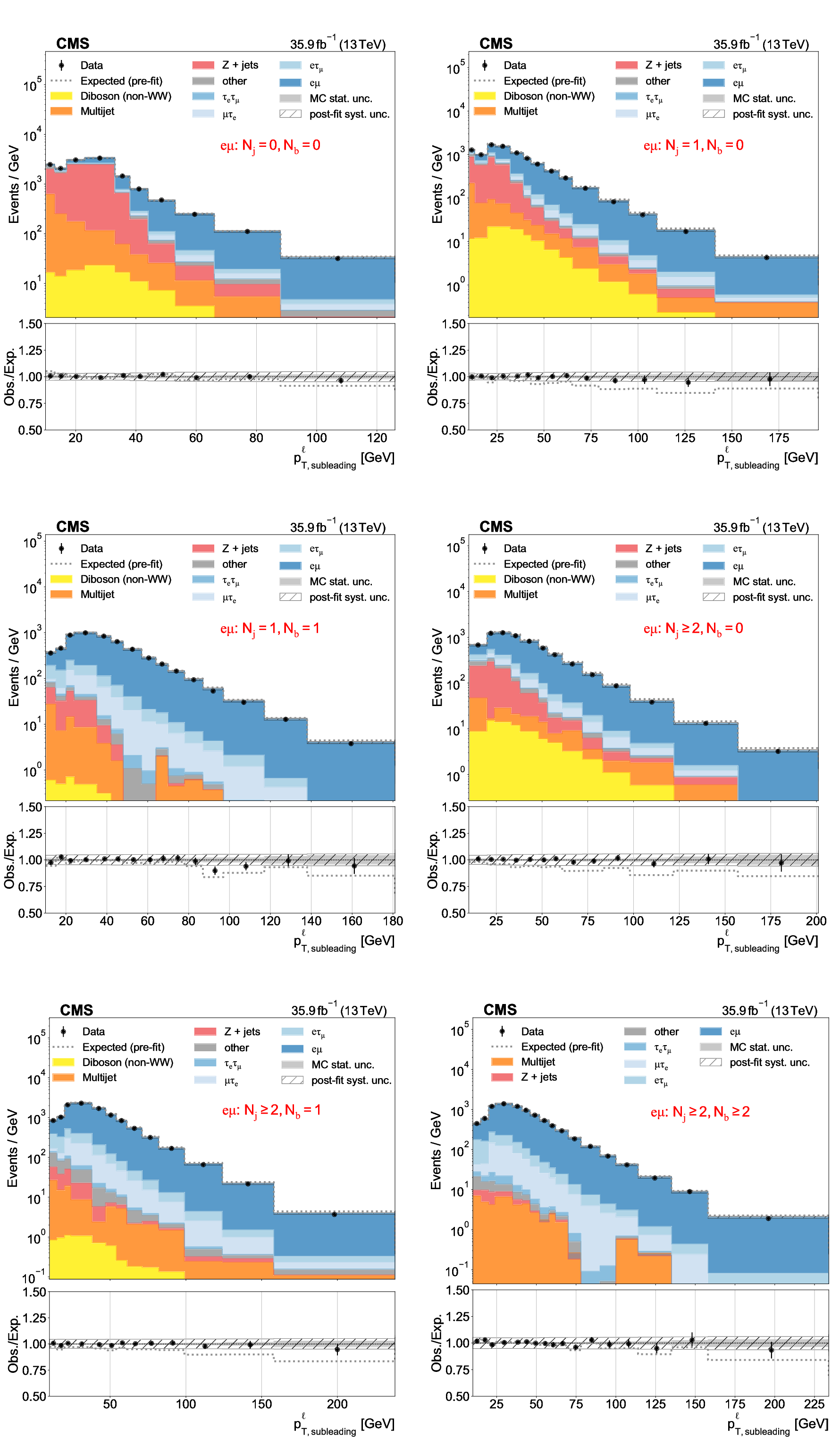
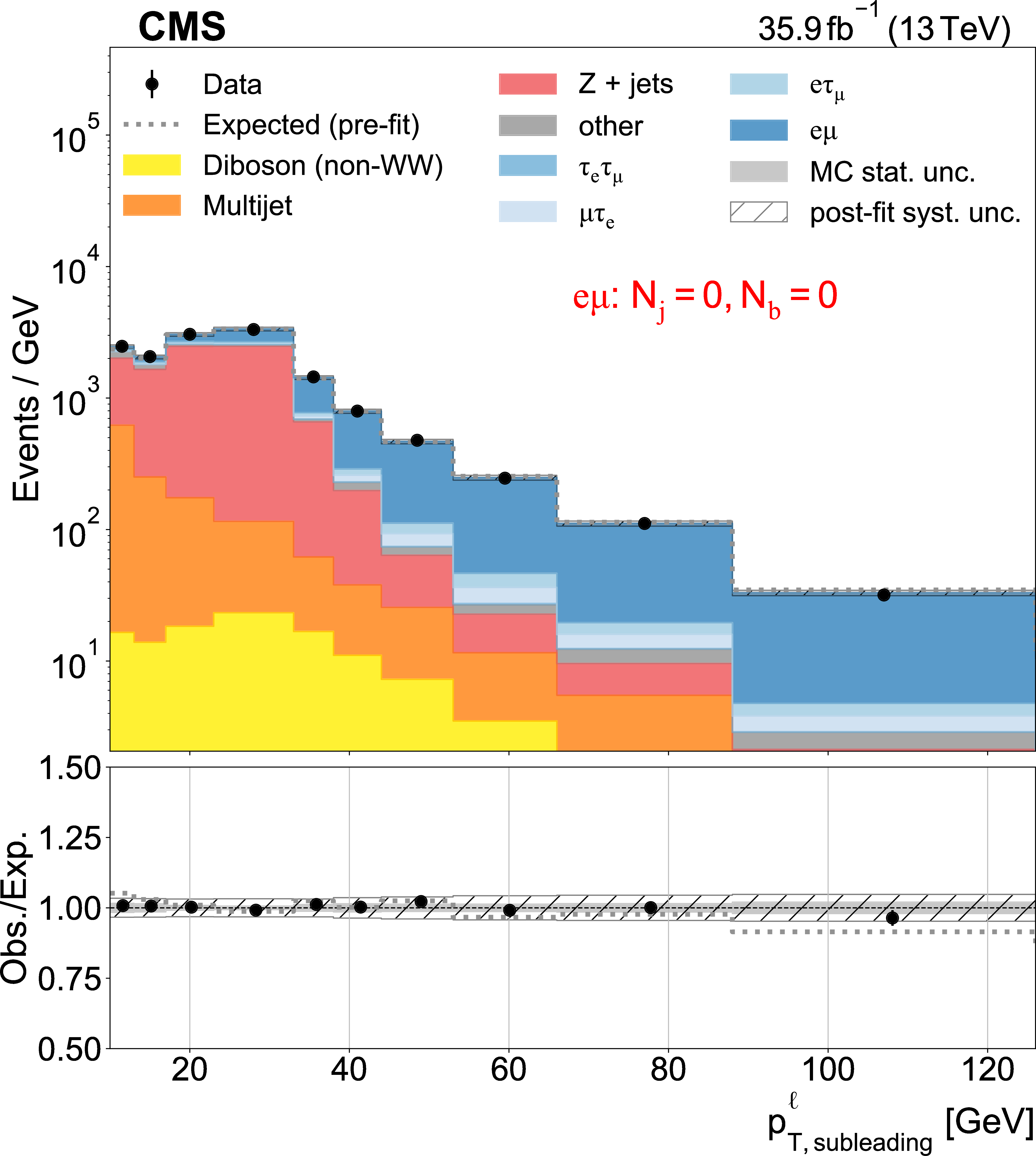
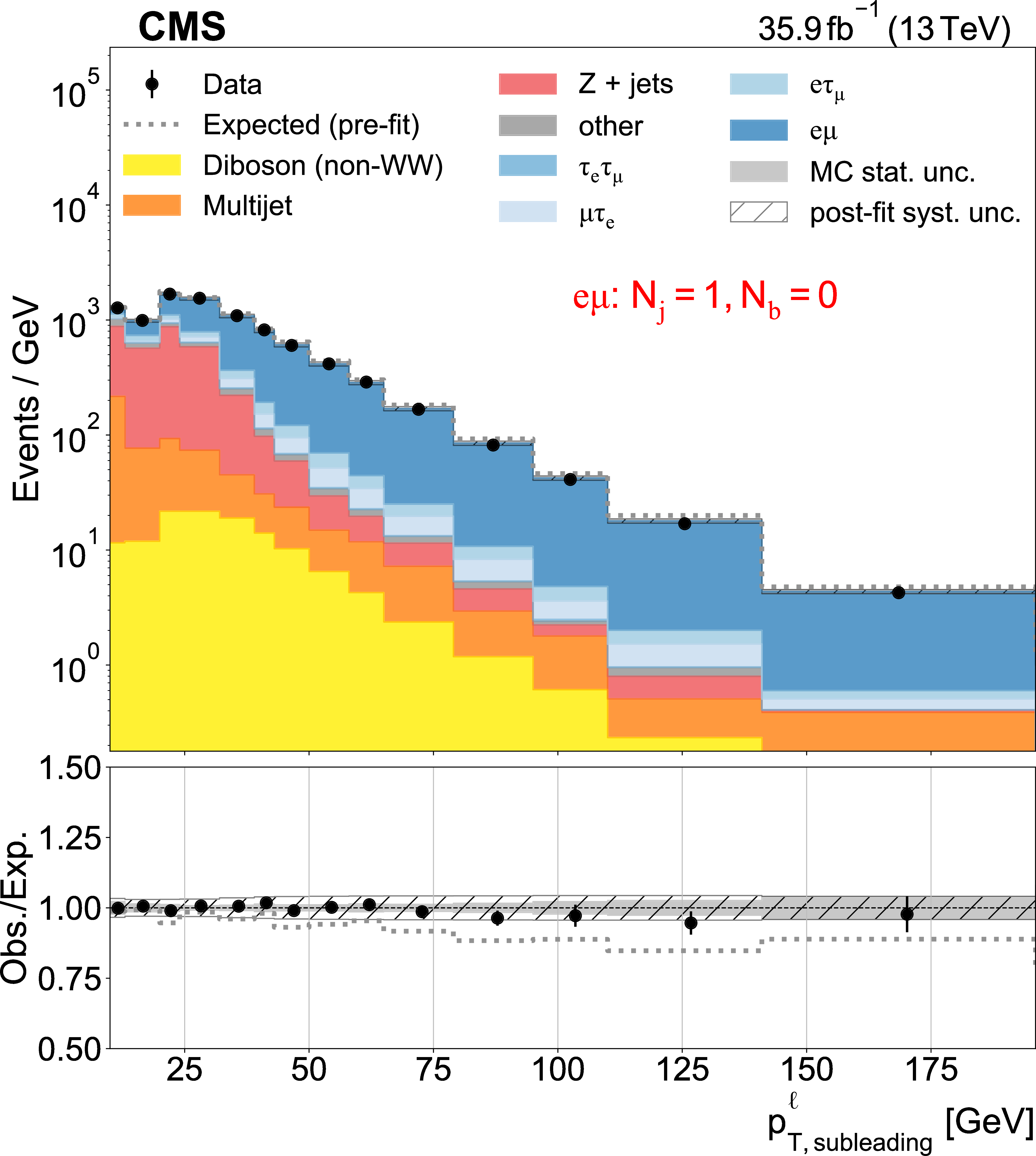
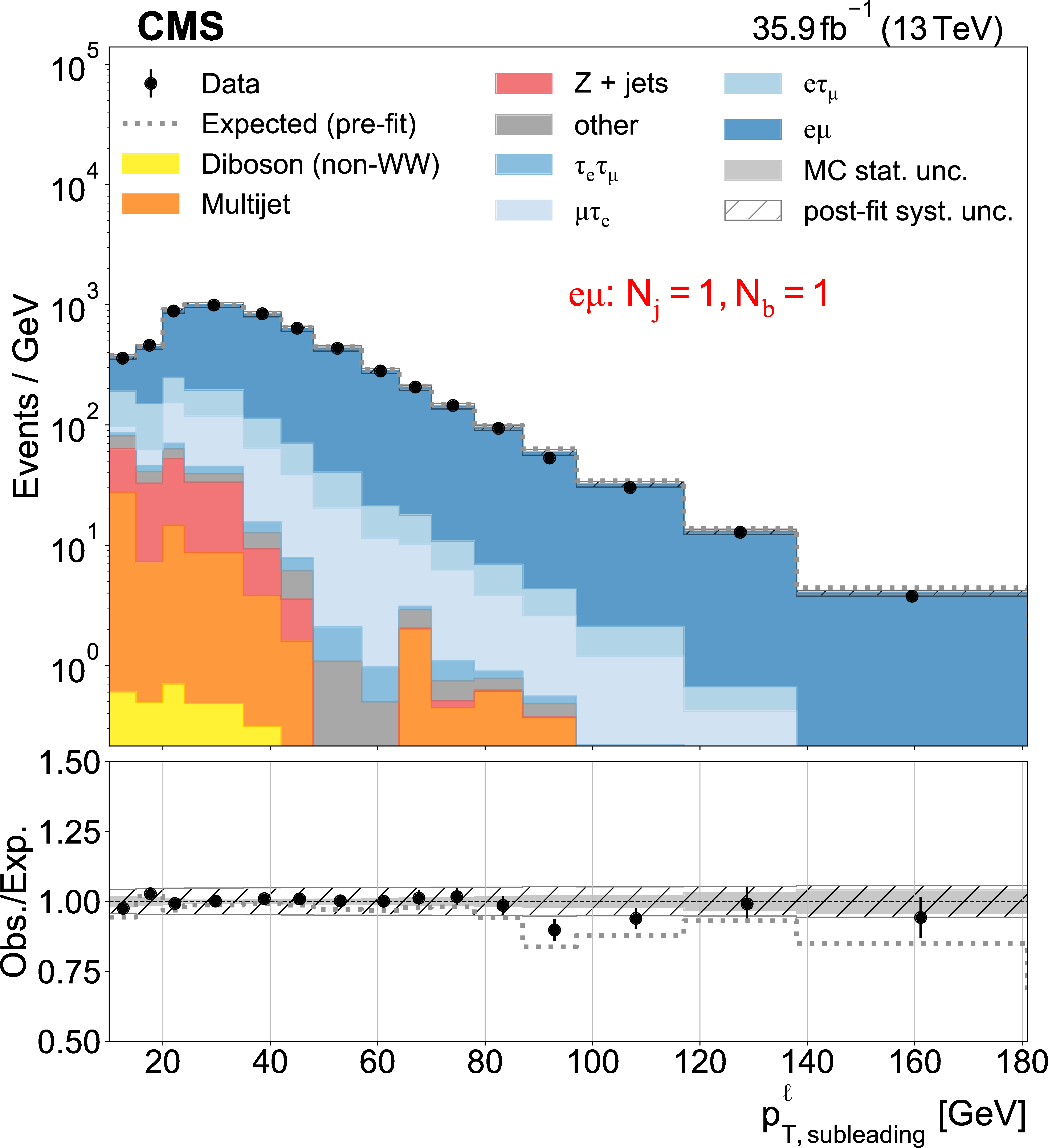
Subleading lepton, electron or muon, ${p_{\mathrm {T}}}$ distributions used as inputs for the binned likelihood fits for the $\mathrm{e} \mu $ categories. The different panels are obtained with the listed selection criteria on the number of jets ($N_{{\text {j}}}$) and of b-tagged jets ($N_{\mathrm{b}}$) required. The lower subpanels show the ratio of data over pre-fit expectations, with the gray histograms (hatched area) indicating MC statistical (post-fit systematic) uncertainties. Vertical bars on the data markers indicate statistical uncertainties. |
png pdf |
Figure 2-a:
Subleading lepton, electron or muon, ${p_{\mathrm {T}}}$ distributions used as inputs for the binned likelihood fits for the $\mathrm{e} \mu $ categories. The different panels are obtained with the listed selection criteria on the number of jets ($N_{{\text {j}}}$) and of b-tagged jets ($N_{\mathrm{b}}$) required. The lower subpanels show the ratio of data over pre-fit expectations, with the gray histograms (hatched area) indicating MC statistical (post-fit systematic) uncertainties. Vertical bars on the data markers indicate statistical uncertainties. |
png pdf |
Figure 2-b:
Subleading lepton, electron or muon, ${p_{\mathrm {T}}}$ distributions used as inputs for the binned likelihood fits for the $\mathrm{e} \mu $ categories. The different panels are obtained with the listed selection criteria on the number of jets ($N_{{\text {j}}}$) and of b-tagged jets ($N_{\mathrm{b}}$) required. The lower subpanels show the ratio of data over pre-fit expectations, with the gray histograms (hatched area) indicating MC statistical (post-fit systematic) uncertainties. Vertical bars on the data markers indicate statistical uncertainties. |
png pdf |
Figure 2-c:
Subleading lepton, electron or muon, ${p_{\mathrm {T}}}$ distributions used as inputs for the binned likelihood fits for the $\mathrm{e} \mu $ categories. The different panels are obtained with the listed selection criteria on the number of jets ($N_{{\text {j}}}$) and of b-tagged jets ($N_{\mathrm{b}}$) required. The lower subpanels show the ratio of data over pre-fit expectations, with the gray histograms (hatched area) indicating MC statistical (post-fit systematic) uncertainties. Vertical bars on the data markers indicate statistical uncertainties. |
png pdf |
Figure 2-d:
Subleading lepton, electron or muon, ${p_{\mathrm {T}}}$ distributions used as inputs for the binned likelihood fits for the $\mathrm{e} \mu $ categories. The different panels are obtained with the listed selection criteria on the number of jets ($N_{{\text {j}}}$) and of b-tagged jets ($N_{\mathrm{b}}$) required. The lower subpanels show the ratio of data over pre-fit expectations, with the gray histograms (hatched area) indicating MC statistical (post-fit systematic) uncertainties. Vertical bars on the data markers indicate statistical uncertainties. |
png pdf |
Figure 2-e:
Subleading lepton, electron or muon, ${p_{\mathrm {T}}}$ distributions used as inputs for the binned likelihood fits for the $\mathrm{e} \mu $ categories. The different panels are obtained with the listed selection criteria on the number of jets ($N_{{\text {j}}}$) and of b-tagged jets ($N_{\mathrm{b}}$) required. The lower subpanels show the ratio of data over pre-fit expectations, with the gray histograms (hatched area) indicating MC statistical (post-fit systematic) uncertainties. Vertical bars on the data markers indicate statistical uncertainties. |
png pdf |
Figure 2-f:
Subleading lepton, electron or muon, ${p_{\mathrm {T}}}$ distributions used as inputs for the binned likelihood fits for the $\mathrm{e} \mu $ categories. The different panels are obtained with the listed selection criteria on the number of jets ($N_{{\text {j}}}$) and of b-tagged jets ($N_{\mathrm{b}}$) required. The lower subpanels show the ratio of data over pre-fit expectations, with the gray histograms (hatched area) indicating MC statistical (post-fit systematic) uncertainties. Vertical bars on the data markers indicate statistical uncertainties. |

png pdf |
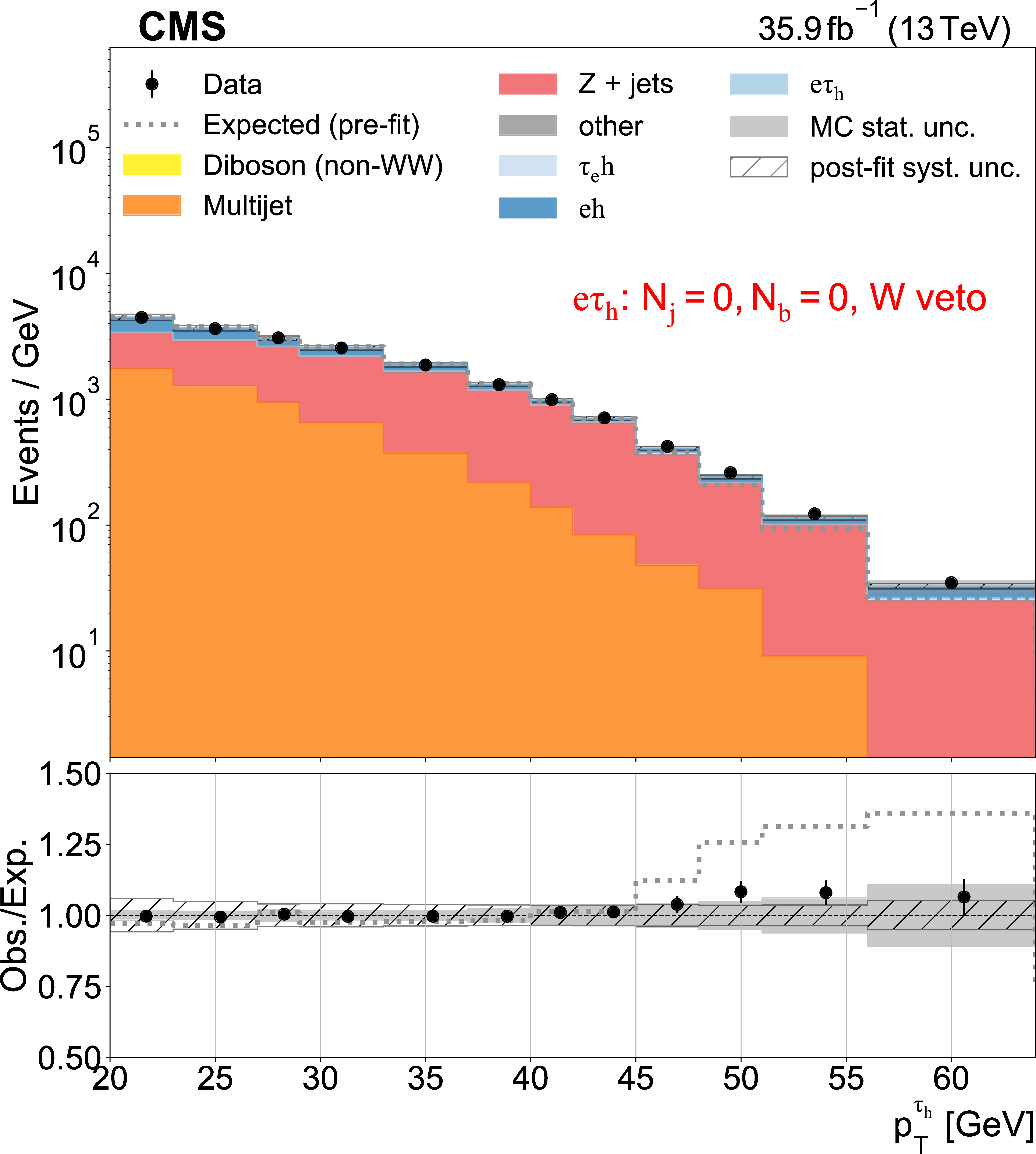
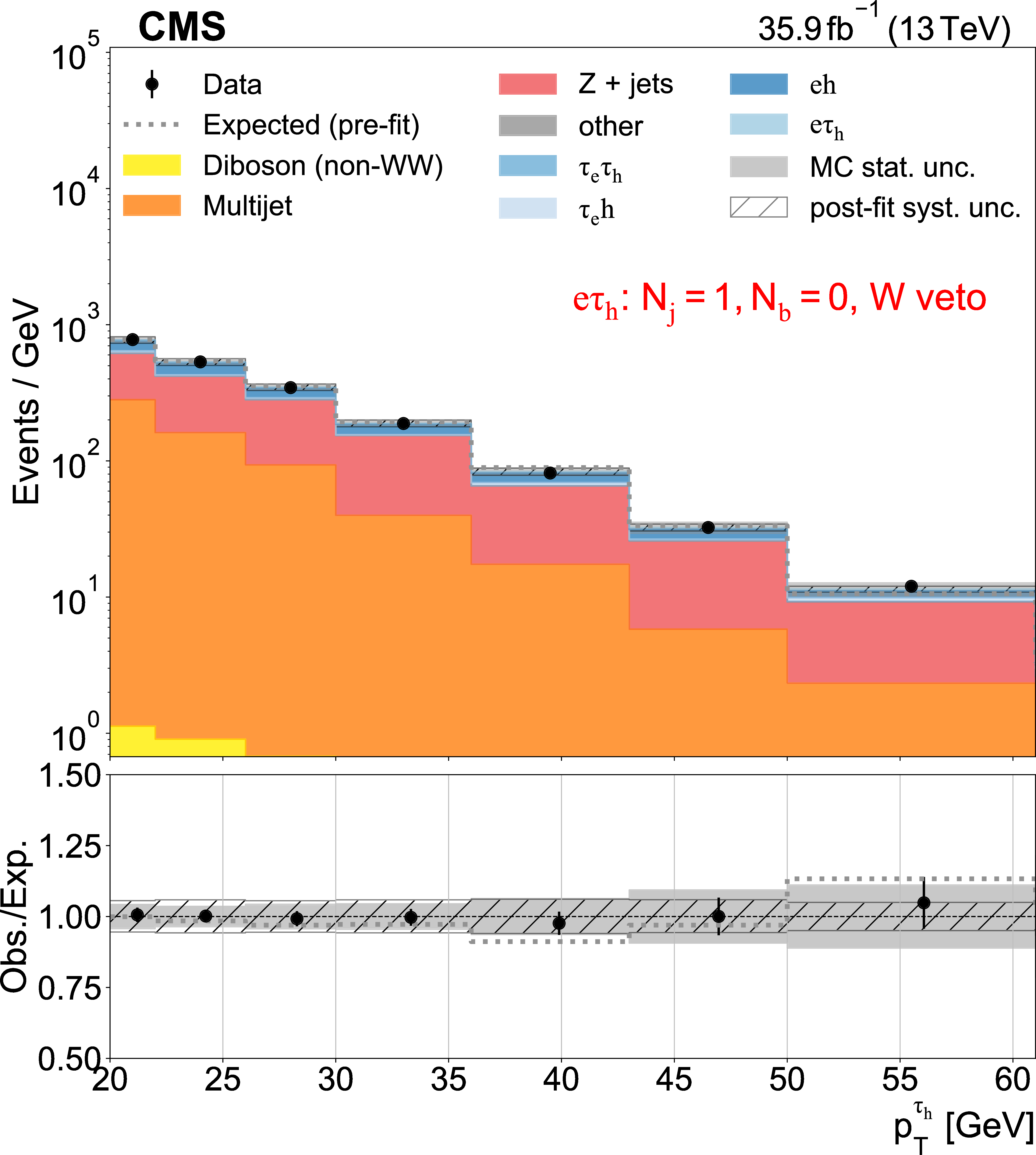
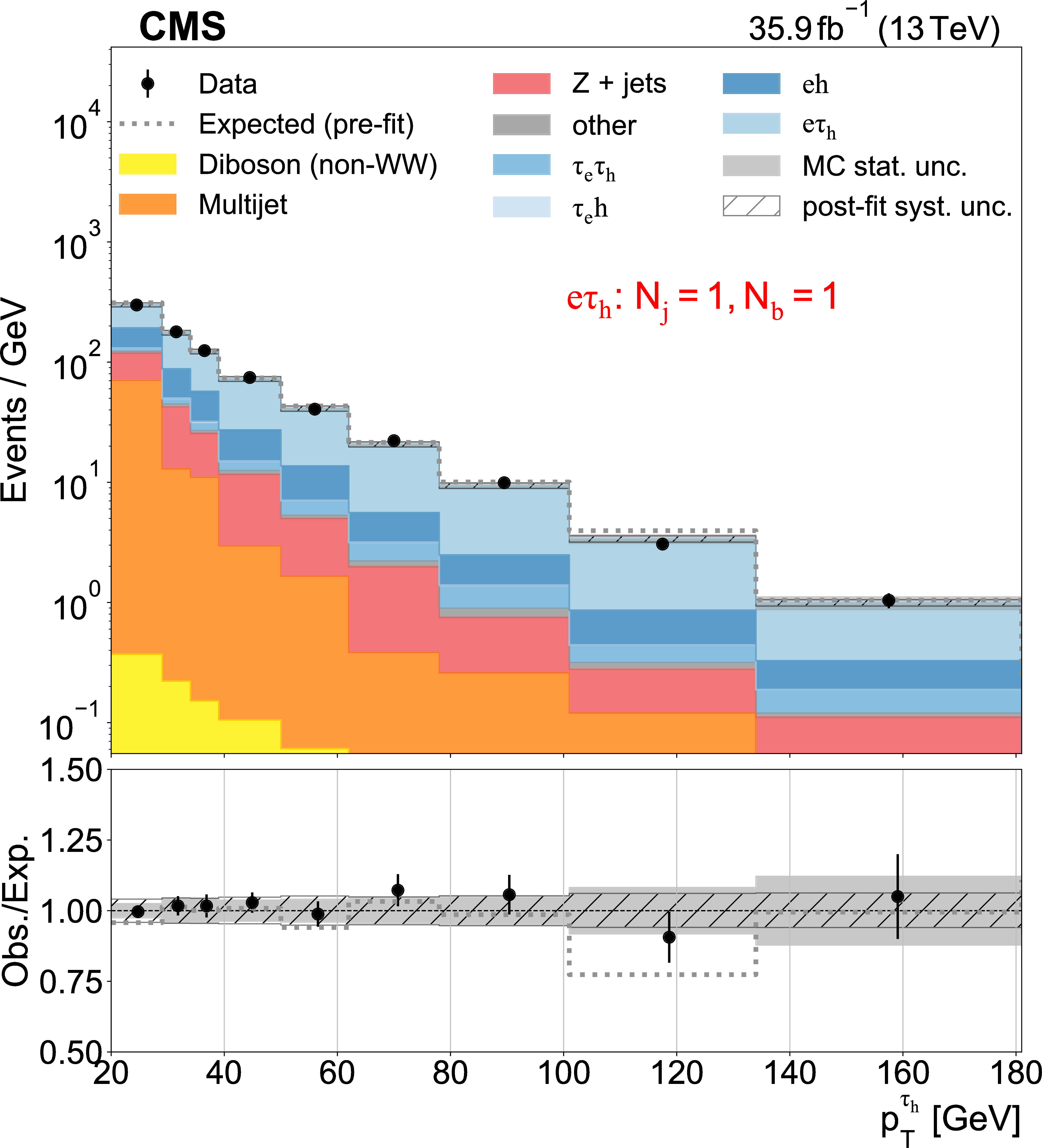
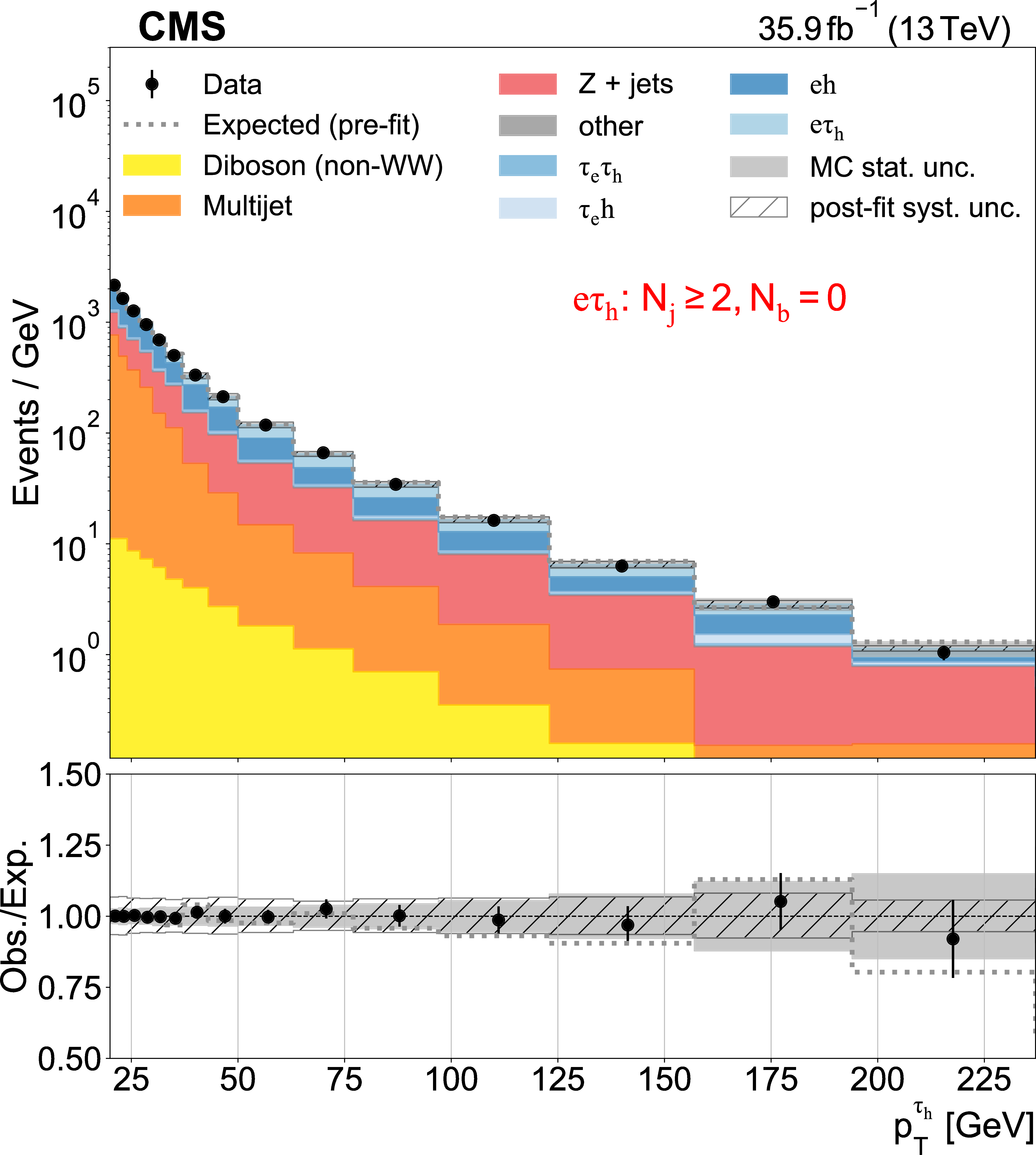
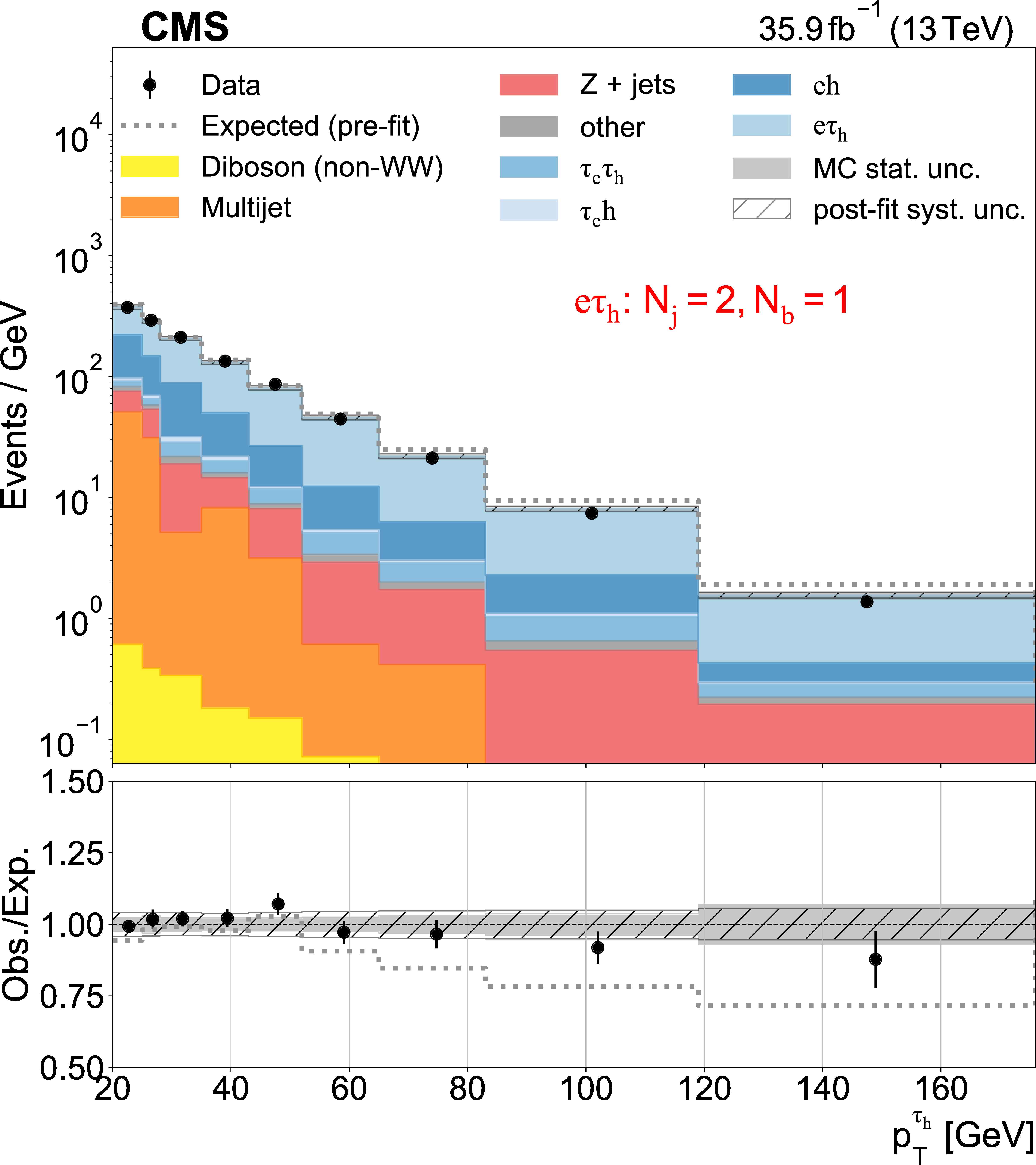
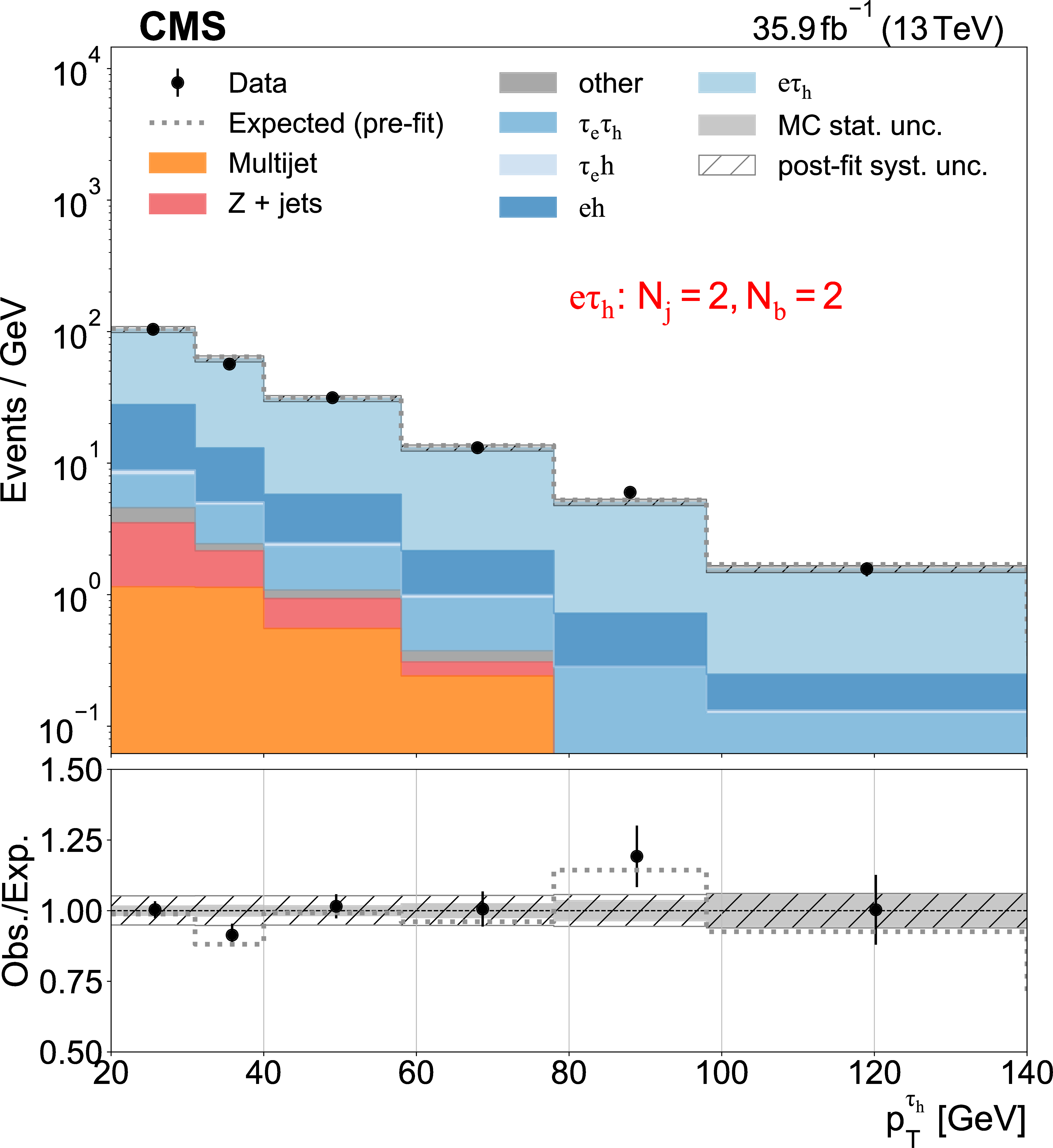
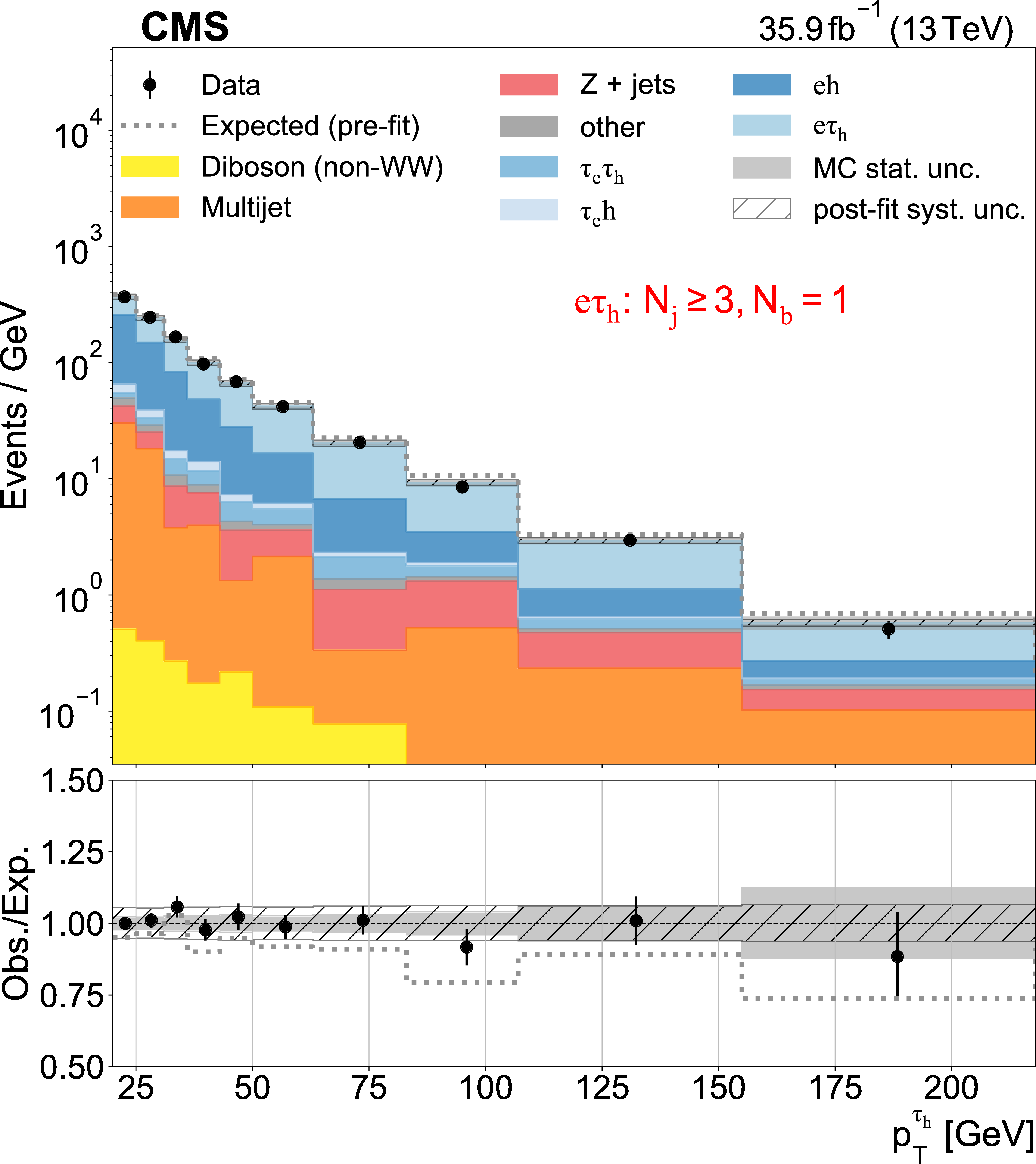
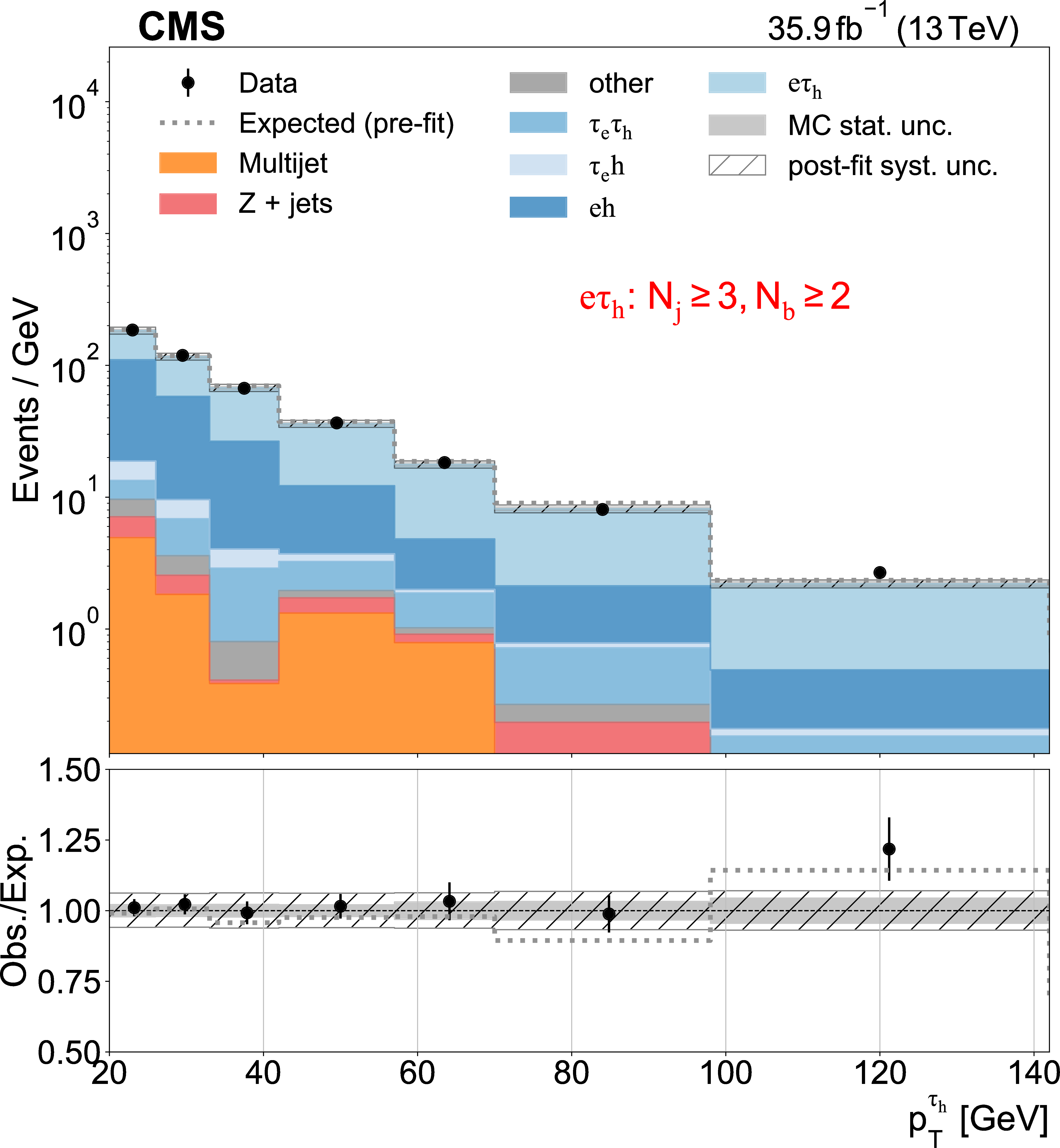
Figure 3:
Distributions of ${\tau _\mathrm {h}}$ ${p_{\mathrm {T}}}$ used as inputs for the binned likelihood fits for the $\mathrm{e} \tau $ categories. The different panels list the varying selections on the number of jets ($N_{{\text {j}}}$) and of b-tagged jets ($N_{\mathrm{b}}$) required in each case. The lower subpanels show the ratio of data over pre-fit expectations, with the gray band (hatched area) indicating MC statistical (post-fit systematic) uncertainties. Vertical bars on the data markers indicate statistical uncertainties. |
png pdf |
Figure 3-a:
Distributions of ${\tau _\mathrm {h}}$ ${p_{\mathrm {T}}}$ used as inputs for the binned likelihood fits for the $\mathrm{e} \tau $ categories. The different panels list the varying selections on the number of jets ($N_{{\text {j}}}$) and of b-tagged jets ($N_{\mathrm{b}}$) required in each case. The lower subpanels show the ratio of data over pre-fit expectations, with the gray band (hatched area) indicating MC statistical (post-fit systematic) uncertainties. Vertical bars on the data markers indicate statistical uncertainties. |
png pdf |
Figure 3-b:
Distributions of ${\tau _\mathrm {h}}$ ${p_{\mathrm {T}}}$ used as inputs for the binned likelihood fits for the $\mathrm{e} \tau $ categories. The different panels list the varying selections on the number of jets ($N_{{\text {j}}}$) and of b-tagged jets ($N_{\mathrm{b}}$) required in each case. The lower subpanels show the ratio of data over pre-fit expectations, with the gray band (hatched area) indicating MC statistical (post-fit systematic) uncertainties. Vertical bars on the data markers indicate statistical uncertainties. |
png pdf |
Figure 3-c:
Distributions of ${\tau _\mathrm {h}}$ ${p_{\mathrm {T}}}$ used as inputs for the binned likelihood fits for the $\mathrm{e} \tau $ categories. The different panels list the varying selections on the number of jets ($N_{{\text {j}}}$) and of b-tagged jets ($N_{\mathrm{b}}$) required in each case. The lower subpanels show the ratio of data over pre-fit expectations, with the gray band (hatched area) indicating MC statistical (post-fit systematic) uncertainties. Vertical bars on the data markers indicate statistical uncertainties. |
png pdf |
Figure 3-d:
Distributions of ${\tau _\mathrm {h}}$ ${p_{\mathrm {T}}}$ used as inputs for the binned likelihood fits for the $\mathrm{e} \tau $ categories. The different panels list the varying selections on the number of jets ($N_{{\text {j}}}$) and of b-tagged jets ($N_{\mathrm{b}}$) required in each case. The lower subpanels show the ratio of data over pre-fit expectations, with the gray band (hatched area) indicating MC statistical (post-fit systematic) uncertainties. Vertical bars on the data markers indicate statistical uncertainties. |
png pdf |
Figure 3-e:
Distributions of ${\tau _\mathrm {h}}$ ${p_{\mathrm {T}}}$ used as inputs for the binned likelihood fits for the $\mathrm{e} \tau $ categories. The different panels list the varying selections on the number of jets ($N_{{\text {j}}}$) and of b-tagged jets ($N_{\mathrm{b}}$) required in each case. The lower subpanels show the ratio of data over pre-fit expectations, with the gray band (hatched area) indicating MC statistical (post-fit systematic) uncertainties. Vertical bars on the data markers indicate statistical uncertainties. |
png pdf |
Figure 3-f:
Distributions of ${\tau _\mathrm {h}}$ ${p_{\mathrm {T}}}$ used as inputs for the binned likelihood fits for the $\mathrm{e} \tau $ categories. The different panels list the varying selections on the number of jets ($N_{{\text {j}}}$) and of b-tagged jets ($N_{\mathrm{b}}$) required in each case. The lower subpanels show the ratio of data over pre-fit expectations, with the gray band (hatched area) indicating MC statistical (post-fit systematic) uncertainties. Vertical bars on the data markers indicate statistical uncertainties. |
png pdf |
Figure 3-g:
Distributions of ${\tau _\mathrm {h}}$ ${p_{\mathrm {T}}}$ used as inputs for the binned likelihood fits for the $\mathrm{e} \tau $ categories. The different panels list the varying selections on the number of jets ($N_{{\text {j}}}$) and of b-tagged jets ($N_{\mathrm{b}}$) required in each case. The lower subpanels show the ratio of data over pre-fit expectations, with the gray band (hatched area) indicating MC statistical (post-fit systematic) uncertainties. Vertical bars on the data markers indicate statistical uncertainties. |
png pdf |
Figure 3-h:
Distributions of ${\tau _\mathrm {h}}$ ${p_{\mathrm {T}}}$ used as inputs for the binned likelihood fits for the $\mathrm{e} \tau $ categories. The different panels list the varying selections on the number of jets ($N_{{\text {j}}}$) and of b-tagged jets ($N_{\mathrm{b}}$) required in each case. The lower subpanels show the ratio of data over pre-fit expectations, with the gray band (hatched area) indicating MC statistical (post-fit systematic) uncertainties. Vertical bars on the data markers indicate statistical uncertainties. |

png pdf |
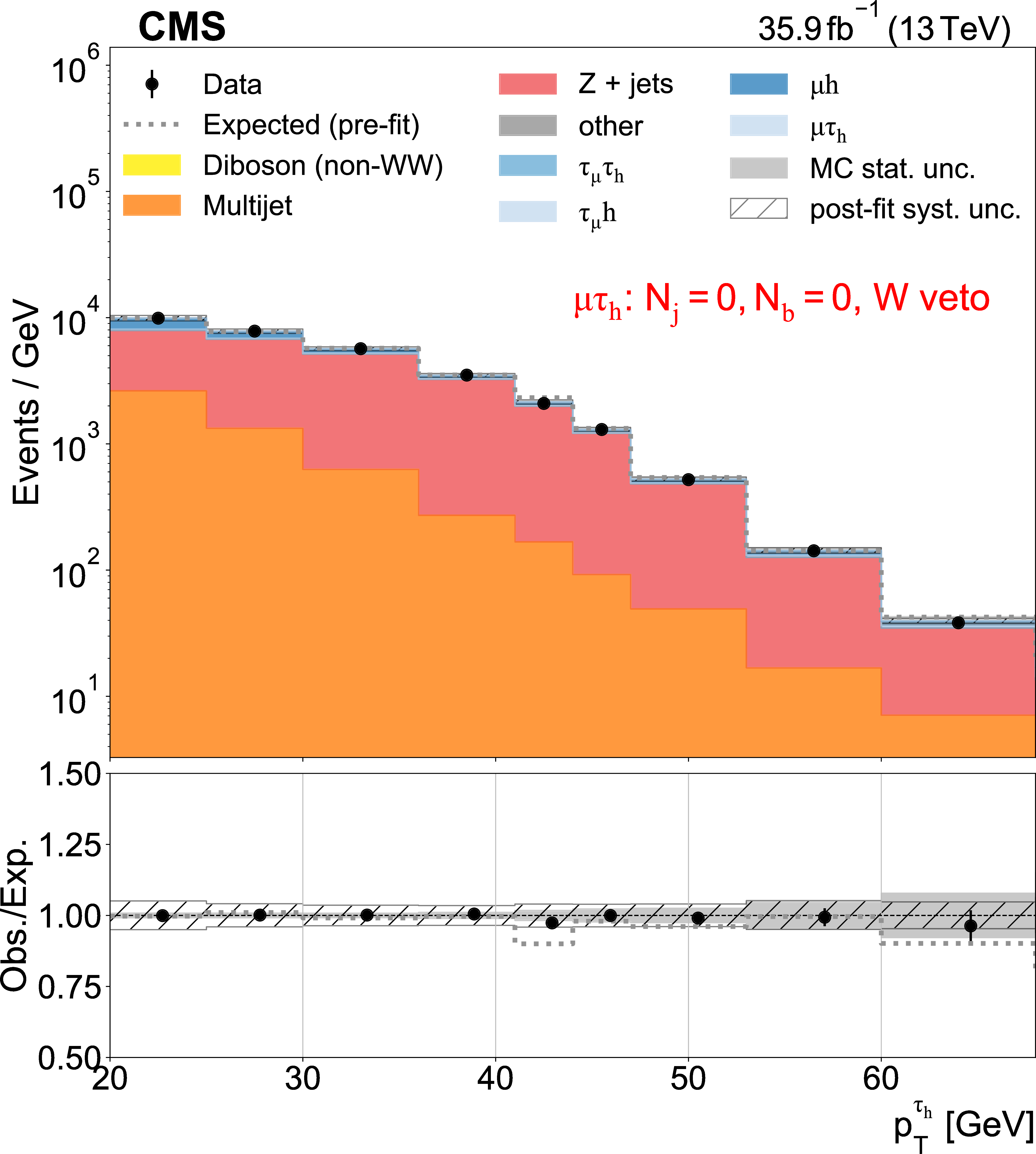
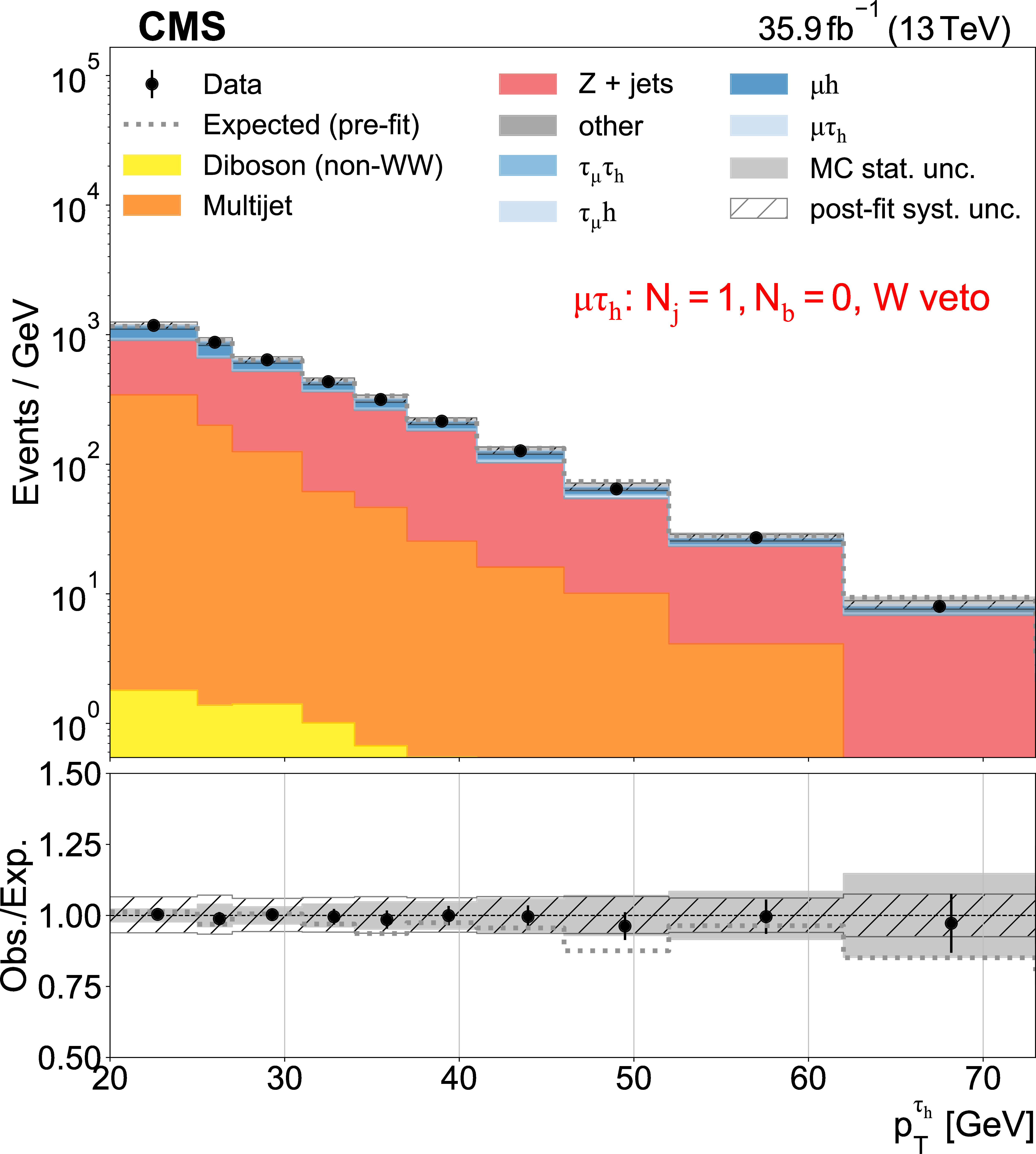
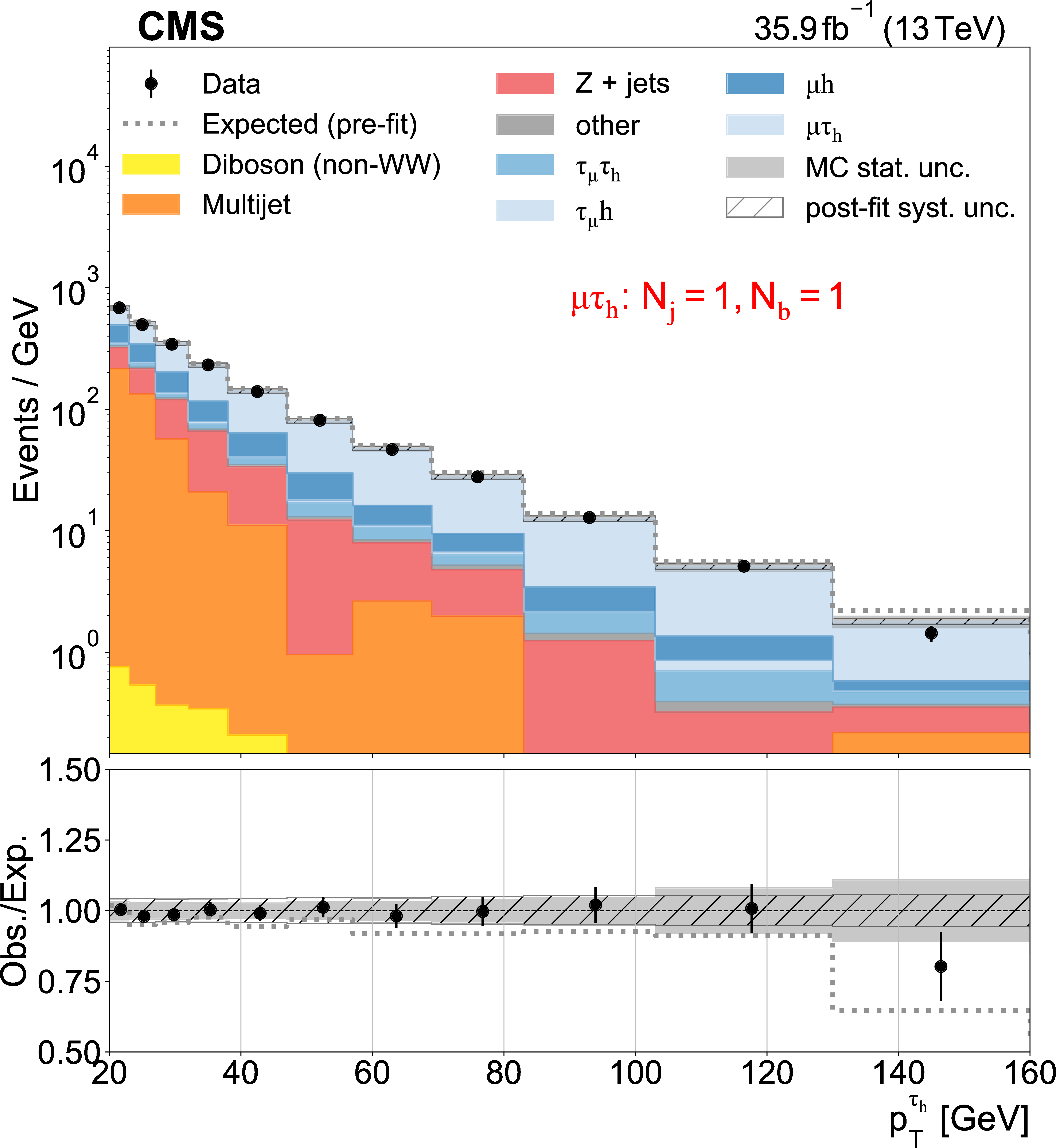
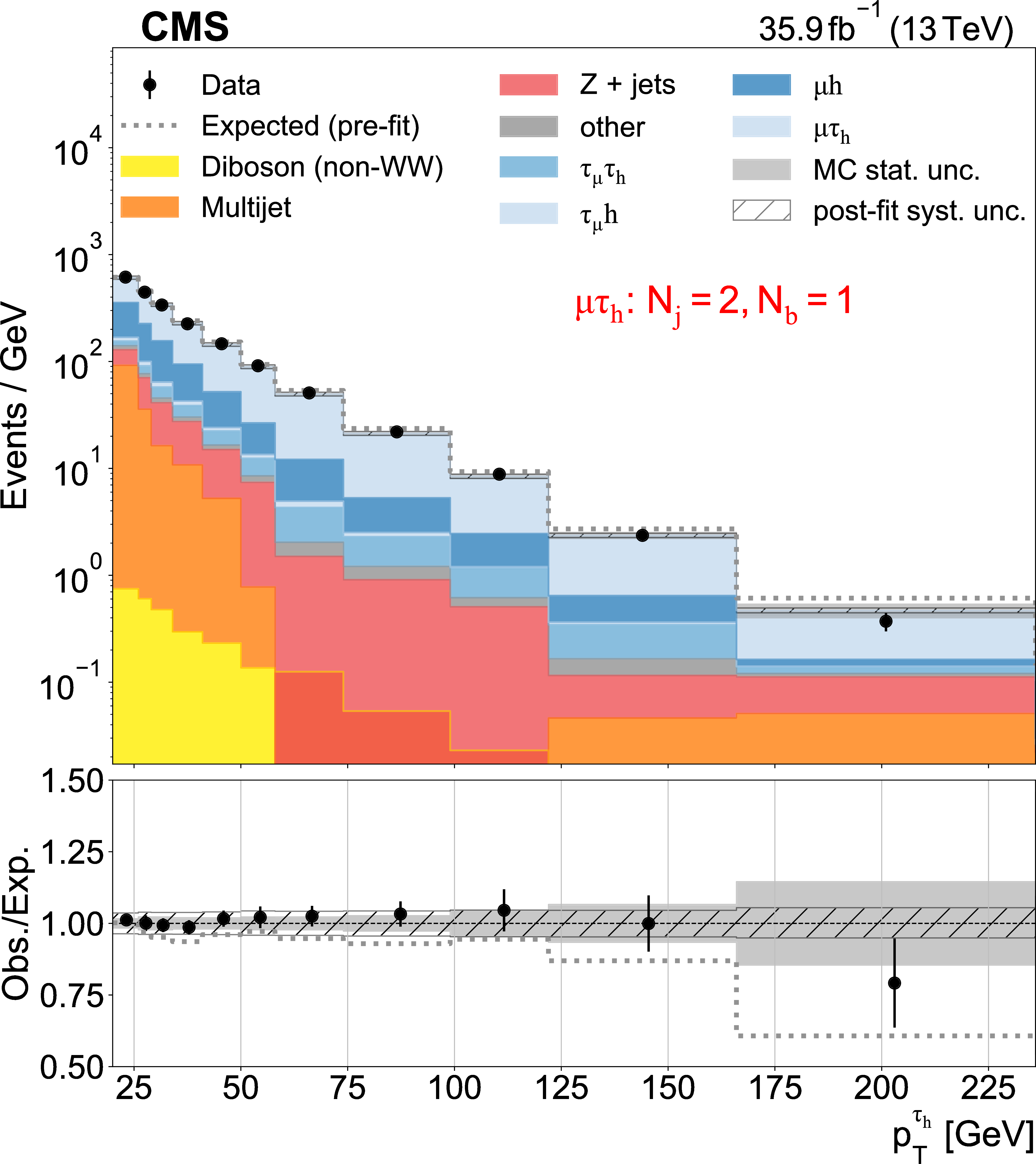
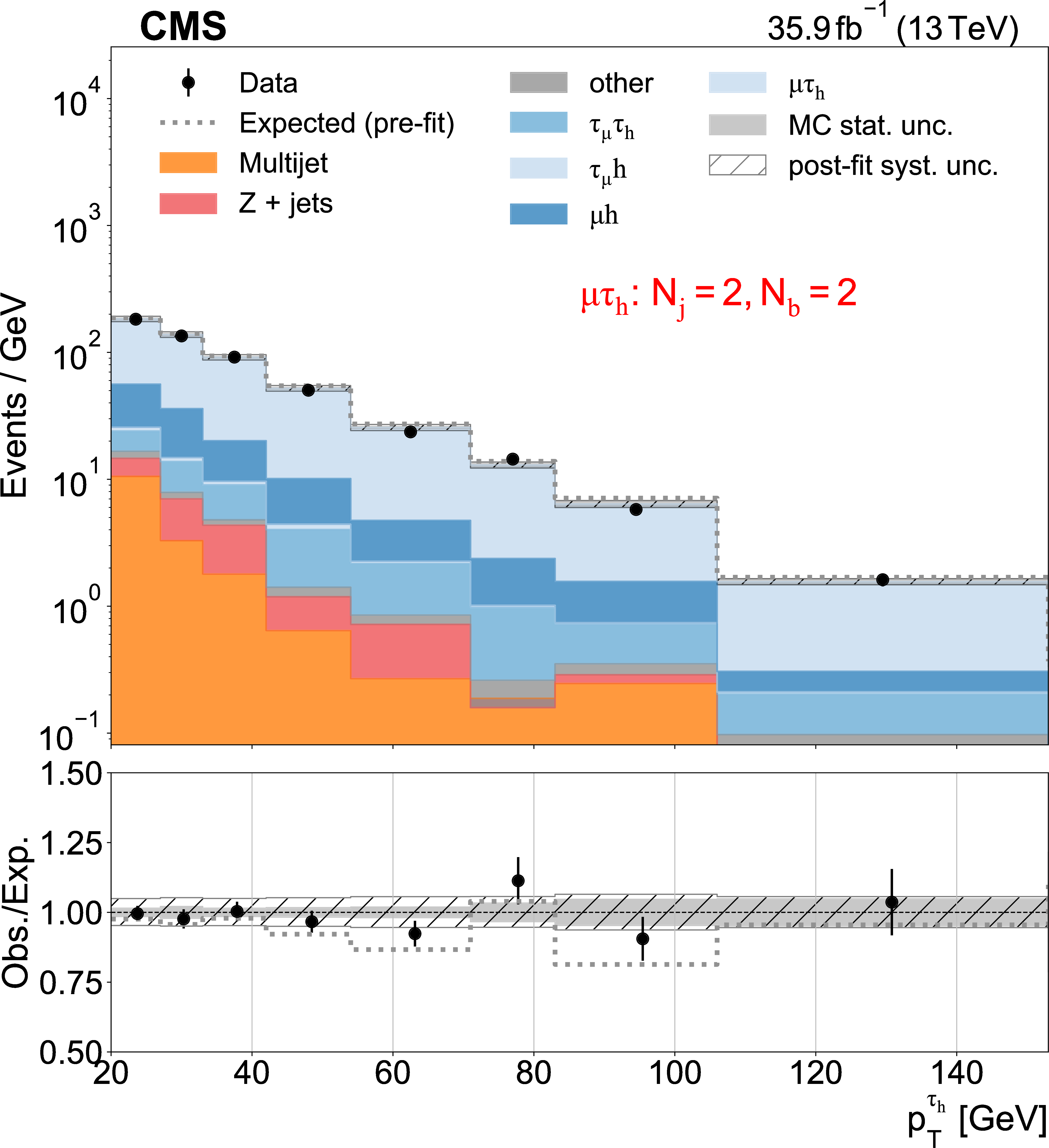
Figure 4:
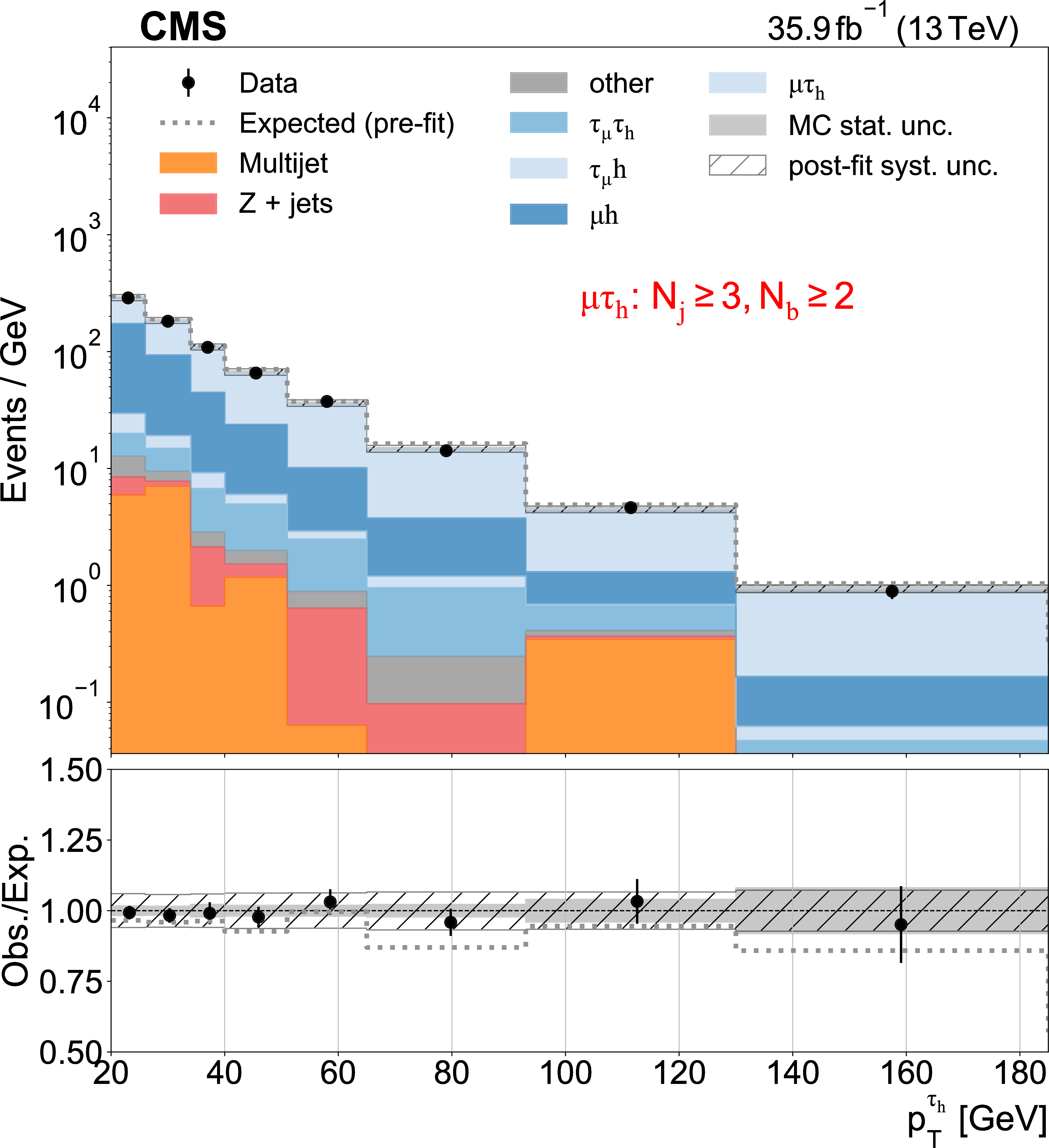
Distributions of ${\tau _\mathrm {h}}$ ${p_{\mathrm {T}}}$ used as inputs for the binned likelihood fits for the $\mu \tau $ categories. The different panels list the varying selections on the number of jets ($N_{{\text {j}}}$) and of b-tagged jets ($N_{\mathrm{b}}$) required in each case. The lower subpanels show the ratio of data over pre-fit expectations, with the gray histograms (hatched area) indicating MC statistical (post-fit systematic) uncertainties. Vertical bars on the data markers indicate statistical uncertainties. |
png pdf |
Figure 4-a:
Distributions of ${\tau _\mathrm {h}}$ ${p_{\mathrm {T}}}$ used as inputs for the binned likelihood fits for the $\mu \tau $ categories. The different panels list the varying selections on the number of jets ($N_{{\text {j}}}$) and of b-tagged jets ($N_{\mathrm{b}}$) required in each case. The lower subpanels show the ratio of data over pre-fit expectations, with the gray histograms (hatched area) indicating MC statistical (post-fit systematic) uncertainties. Vertical bars on the data markers indicate statistical uncertainties. |
png pdf |
Figure 4-b:
Distributions of ${\tau _\mathrm {h}}$ ${p_{\mathrm {T}}}$ used as inputs for the binned likelihood fits for the $\mu \tau $ categories. The different panels list the varying selections on the number of jets ($N_{{\text {j}}}$) and of b-tagged jets ($N_{\mathrm{b}}$) required in each case. The lower subpanels show the ratio of data over pre-fit expectations, with the gray histograms (hatched area) indicating MC statistical (post-fit systematic) uncertainties. Vertical bars on the data markers indicate statistical uncertainties. |
png pdf |
Figure 4-c:
Distributions of ${\tau _\mathrm {h}}$ ${p_{\mathrm {T}}}$ used as inputs for the binned likelihood fits for the $\mu \tau $ categories. The different panels list the varying selections on the number of jets ($N_{{\text {j}}}$) and of b-tagged jets ($N_{\mathrm{b}}$) required in each case. The lower subpanels show the ratio of data over pre-fit expectations, with the gray histograms (hatched area) indicating MC statistical (post-fit systematic) uncertainties. Vertical bars on the data markers indicate statistical uncertainties. |

png pdf |
Figure 4-d:
Distributions of ${\tau _\mathrm {h}}$ ${p_{\mathrm {T}}}$ used as inputs for the binned likelihood fits for the $\mu \tau $ categories. The different panels list the varying selections on the number of jets ($N_{{\text {j}}}$) and of b-tagged jets ($N_{\mathrm{b}}$) required in each case. The lower subpanels show the ratio of data over pre-fit expectations, with the gray histograms (hatched area) indicating MC statistical (post-fit systematic) uncertainties. Vertical bars on the data markers indicate statistical uncertainties. |
png pdf |
Figure 4-e:
Distributions of ${\tau _\mathrm {h}}$ ${p_{\mathrm {T}}}$ used as inputs for the binned likelihood fits for the $\mu \tau $ categories. The different panels list the varying selections on the number of jets ($N_{{\text {j}}}$) and of b-tagged jets ($N_{\mathrm{b}}$) required in each case. The lower subpanels show the ratio of data over pre-fit expectations, with the gray histograms (hatched area) indicating MC statistical (post-fit systematic) uncertainties. Vertical bars on the data markers indicate statistical uncertainties. |
png pdf |
Figure 4-f:
Distributions of ${\tau _\mathrm {h}}$ ${p_{\mathrm {T}}}$ used as inputs for the binned likelihood fits for the $\mu \tau $ categories. The different panels list the varying selections on the number of jets ($N_{{\text {j}}}$) and of b-tagged jets ($N_{\mathrm{b}}$) required in each case. The lower subpanels show the ratio of data over pre-fit expectations, with the gray histograms (hatched area) indicating MC statistical (post-fit systematic) uncertainties. Vertical bars on the data markers indicate statistical uncertainties. |

png pdf |
Figure 4-g:
Distributions of ${\tau _\mathrm {h}}$ ${p_{\mathrm {T}}}$ used as inputs for the binned likelihood fits for the $\mu \tau $ categories. The different panels list the varying selections on the number of jets ($N_{{\text {j}}}$) and of b-tagged jets ($N_{\mathrm{b}}$) required in each case. The lower subpanels show the ratio of data over pre-fit expectations, with the gray histograms (hatched area) indicating MC statistical (post-fit systematic) uncertainties. Vertical bars on the data markers indicate statistical uncertainties. |
png pdf |
Figure 4-h:
Distributions of ${\tau _\mathrm {h}}$ ${p_{\mathrm {T}}}$ used as inputs for the binned likelihood fits for the $\mu \tau $ categories. The different panels list the varying selections on the number of jets ($N_{{\text {j}}}$) and of b-tagged jets ($N_{\mathrm{b}}$) required in each case. The lower subpanels show the ratio of data over pre-fit expectations, with the gray histograms (hatched area) indicating MC statistical (post-fit systematic) uncertainties. Vertical bars on the data markers indicate statistical uncertainties. |

png pdf |
Figure 5:
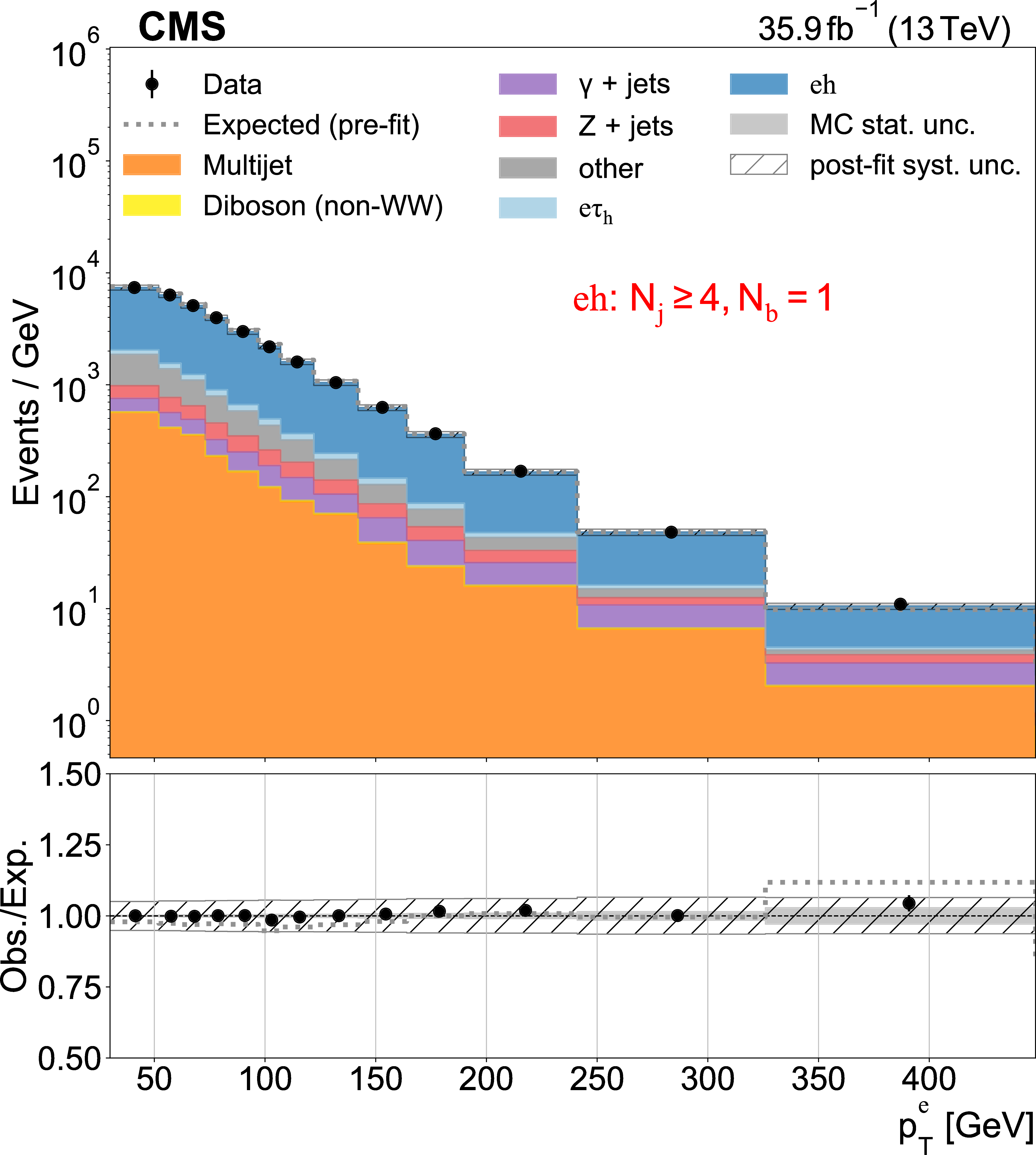
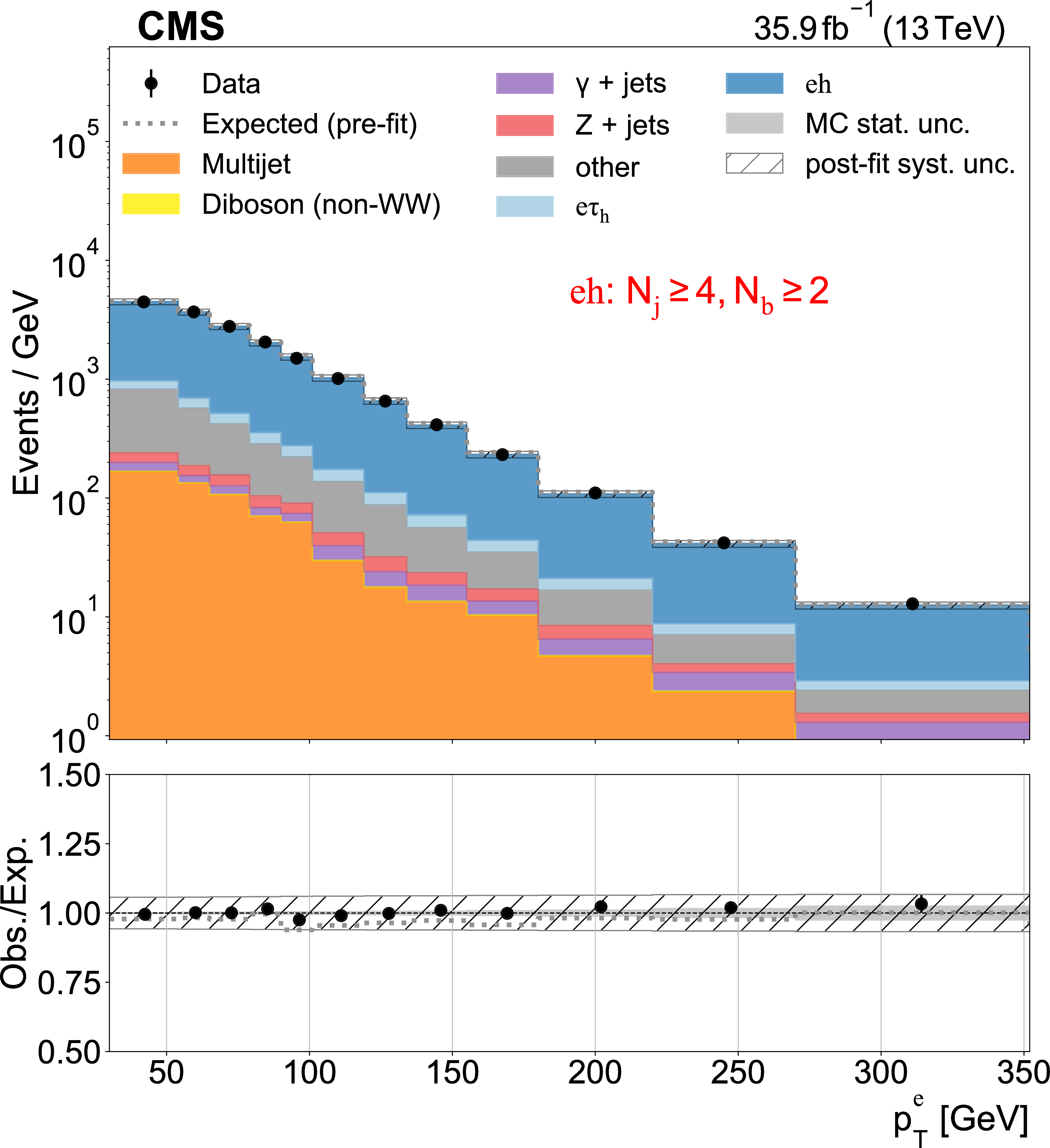
Distributions of electron or muon ${p_{\mathrm {T}}}$ used as inputs for the binned likelihood fits for the $\mathrm{e} {\text {h}} $ (upper) and $\mu {\text {h}} $ (lower) categories, respectively, with the requirement of one (left) or more than one (right) b-tagged jets. The lower subpanels show the ratio of data over pre-fit expectations, with the gray histograms (hatched area) indicating MC statistical (post-fit systematic) uncertainties. Vertical bars on the data markers indicate statistical uncertainties. |
png pdf |
Figure 5-a:
Distributions of electron or muon ${p_{\mathrm {T}}}$ used as inputs for the binned likelihood fits for the $\mathrm{e} {\text {h}} $ (upper) and $\mu {\text {h}} $ (lower) categories, respectively, with the requirement of one (left) or more than one (right) b-tagged jets. The lower subpanels show the ratio of data over pre-fit expectations, with the gray histograms (hatched area) indicating MC statistical (post-fit systematic) uncertainties. Vertical bars on the data markers indicate statistical uncertainties. |
png pdf |
Figure 5-b:
Distributions of electron or muon ${p_{\mathrm {T}}}$ used as inputs for the binned likelihood fits for the $\mathrm{e} {\text {h}} $ (upper) and $\mu {\text {h}} $ (lower) categories, respectively, with the requirement of one (left) or more than one (right) b-tagged jets. The lower subpanels show the ratio of data over pre-fit expectations, with the gray histograms (hatched area) indicating MC statistical (post-fit systematic) uncertainties. Vertical bars on the data markers indicate statistical uncertainties. |

png pdf |
Figure 5-c:
Distributions of electron or muon ${p_{\mathrm {T}}}$ used as inputs for the binned likelihood fits for the $\mathrm{e} {\text {h}} $ (upper) and $\mu {\text {h}} $ (lower) categories, respectively, with the requirement of one (left) or more than one (right) b-tagged jets. The lower subpanels show the ratio of data over pre-fit expectations, with the gray histograms (hatched area) indicating MC statistical (post-fit systematic) uncertainties. Vertical bars on the data markers indicate statistical uncertainties. |

png pdf |
Figure 5-d:
Distributions of electron or muon ${p_{\mathrm {T}}}$ used as inputs for the binned likelihood fits for the $\mathrm{e} {\text {h}} $ (upper) and $\mu {\text {h}} $ (lower) categories, respectively, with the requirement of one (left) or more than one (right) b-tagged jets. The lower subpanels show the ratio of data over pre-fit expectations, with the gray histograms (hatched area) indicating MC statistical (post-fit systematic) uncertainties. Vertical bars on the data markers indicate statistical uncertainties. |
png pdf |
Figure 6:
Summary of the measured values of the W leptonic branching fractions compared with the corresponding LEP results [8,9]. The vertical green-yellow band shows the extracted W leptonic branching fraction assuming LFU (the hatched band shows the corresponding LEP result). The horizontal error bars on the data points indicate their total uncertainty. |

png pdf |
Figure 7:
Two-dimensional distributions of pairs of W leptonic branching fractions derived here compared with the corresponding LEP results [8,9] and to the SM expectation. The green (darker) and yellow (lighter) bands (dashed lines for the LEP results) correspond to the 68% and 95% CL, respectively, for the resulting two-dimensional Gaussian distribution. |
png pdf |
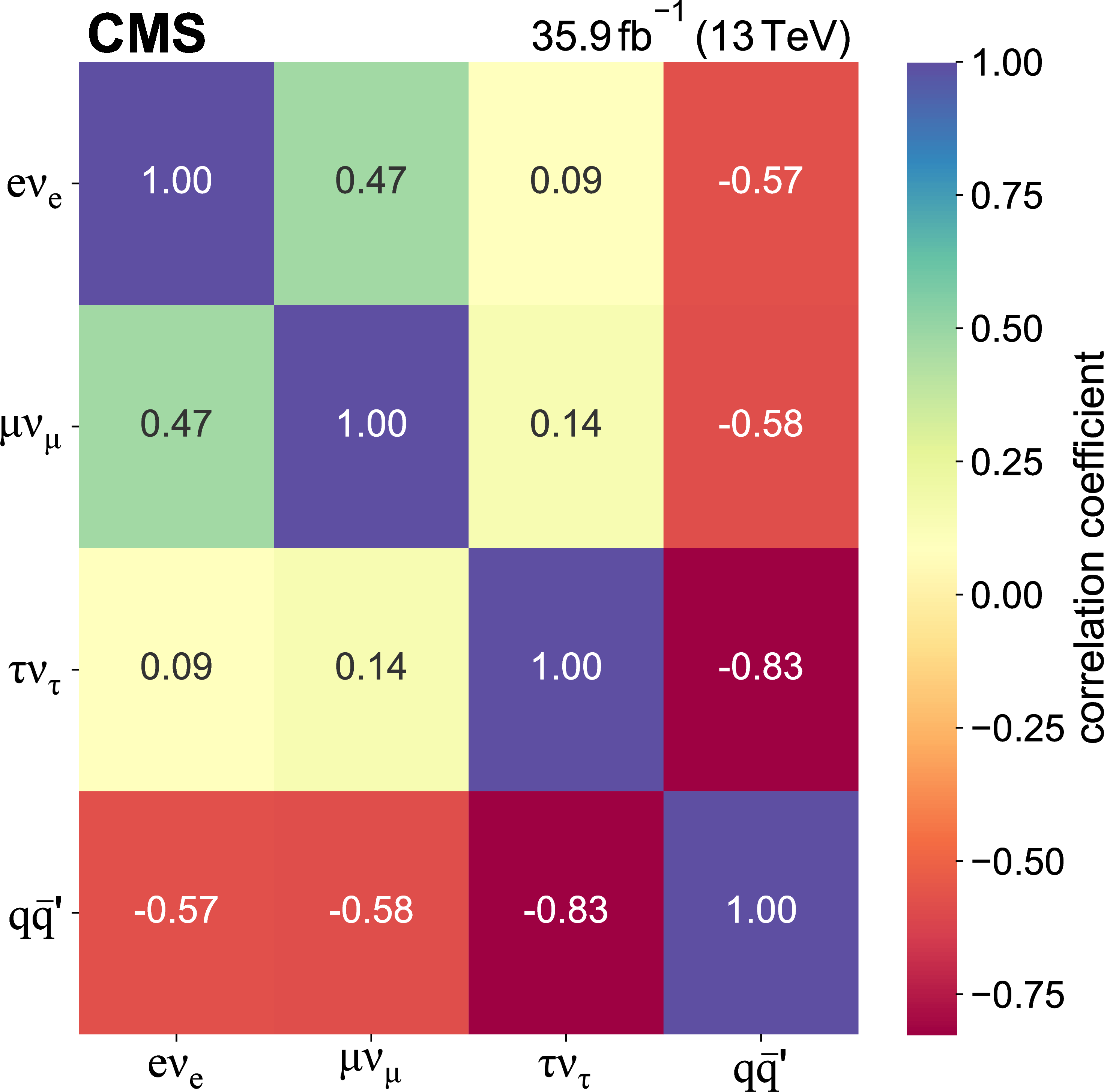
Figure 8:
Correlation matrix between the four W boson decay branching fraction components extracted in this work. |
png pdf |
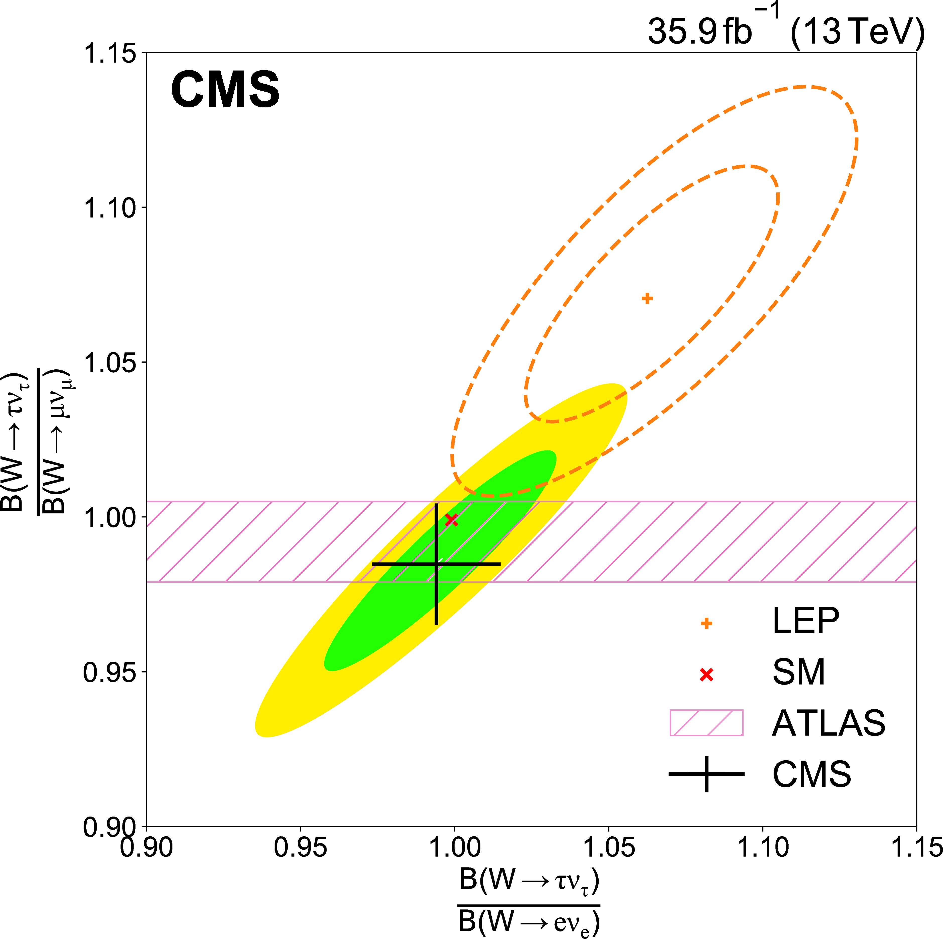
Figure 9:
Two-dimensional distribution of the ratio ${R_{\tau /\mathrm{e}}}$ versus ${R_{\tau /\mu}}$, compared with the corresponding LEP [8,9] and ATLAS [13] results and with the SM expectation. The green and yellow bands (dashed lines for the LEP results) correspond to the 68% and 95% CL, respectively, for the resulting two-dimensional Gaussian distribution. The corresponding 68% CL one-dimensional projections (black error bars) are also overlaid for a better visual comparison with the ATLAS ${R_{\tau /\mu}}$ result. |
| Tables | |
png pdf |
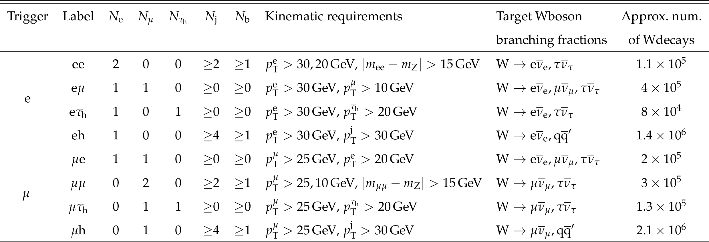
Table 1:
Categorization of events based on the triggering lepton, the number of reconstructed and selected leptons ($N_{\mathrm{e}}$, $N_{\mu}$, $N_{{\tau _\mathrm {h}}}$), number of jets ($N_ {\text {j}} $), and number of b-tagged jets ($N_{\mathrm{b}}$). Kinematic requirements of the leptons and jets are listed in the fourth column. Categories with two leptons in the final state require the selected leptons to have opposite signs. The second-to-last column lists the targeted W boson branching fractions, and the last column provides the approximate number of W decays collected in each category. |
png pdf |
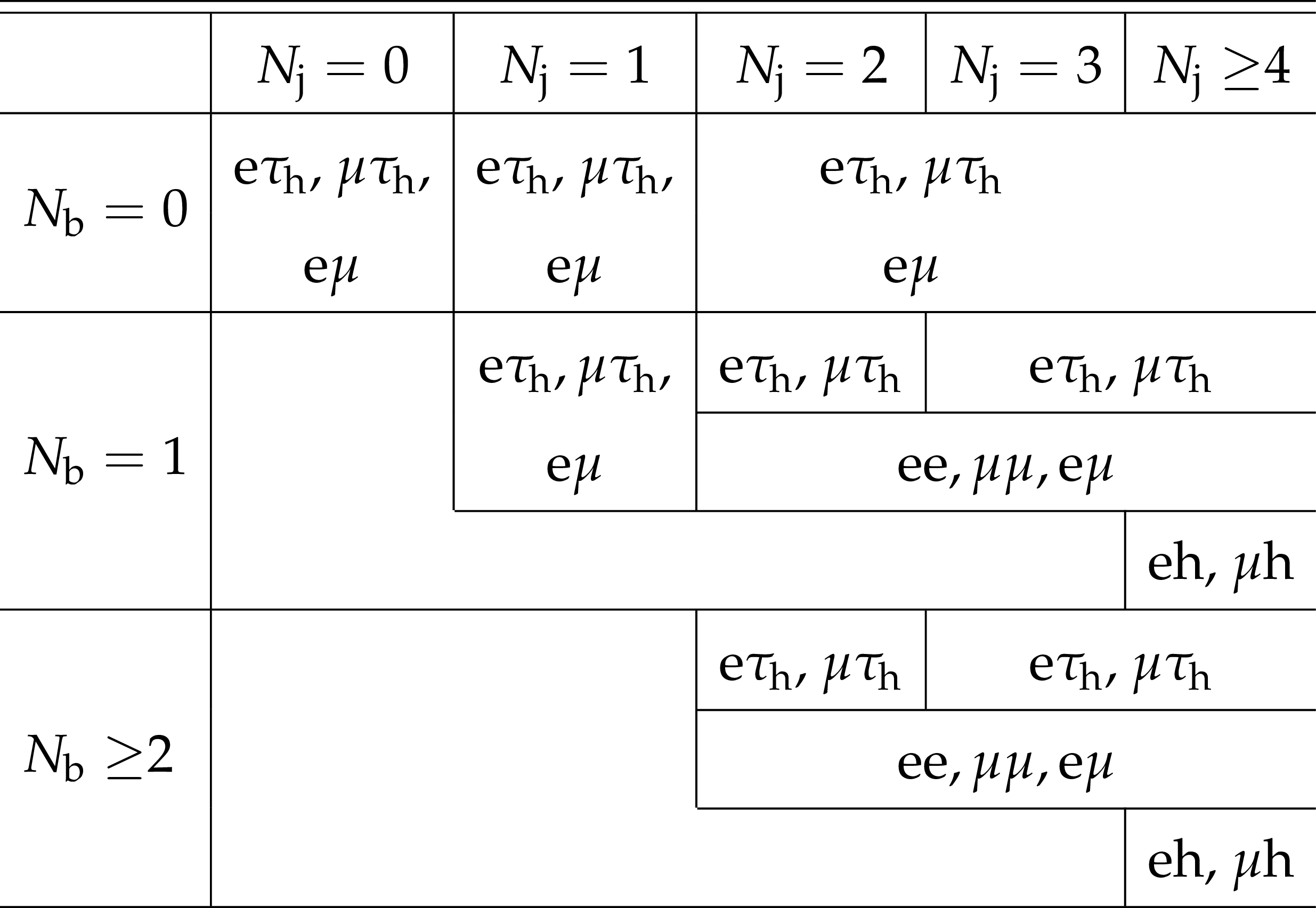
Table 2:
Categorization of events with electrons, muons, and ${\tau _\mathrm {h}}$ passing the reconstruction criteria, based on their jet and b-tagged jet multiplicities, used to define signal-enriched and control regions. Events in the $\mathrm{e} {\tau _\mathrm {h}} $ and $\mu {\tau _\mathrm {h}} $ categories with at least one jet that is not b-tagged are additionally required to satisfy 40 $\leq m_{\ell {\tau _\mathrm {h}}} \leq $ 100 GeV, $\Delta \phi (\ell, {\tau _\mathrm {h}}) > $ 2.5, and $ {m_{\mathrm {T}}} ^\ell < $ 60 GeV. |
png pdf |
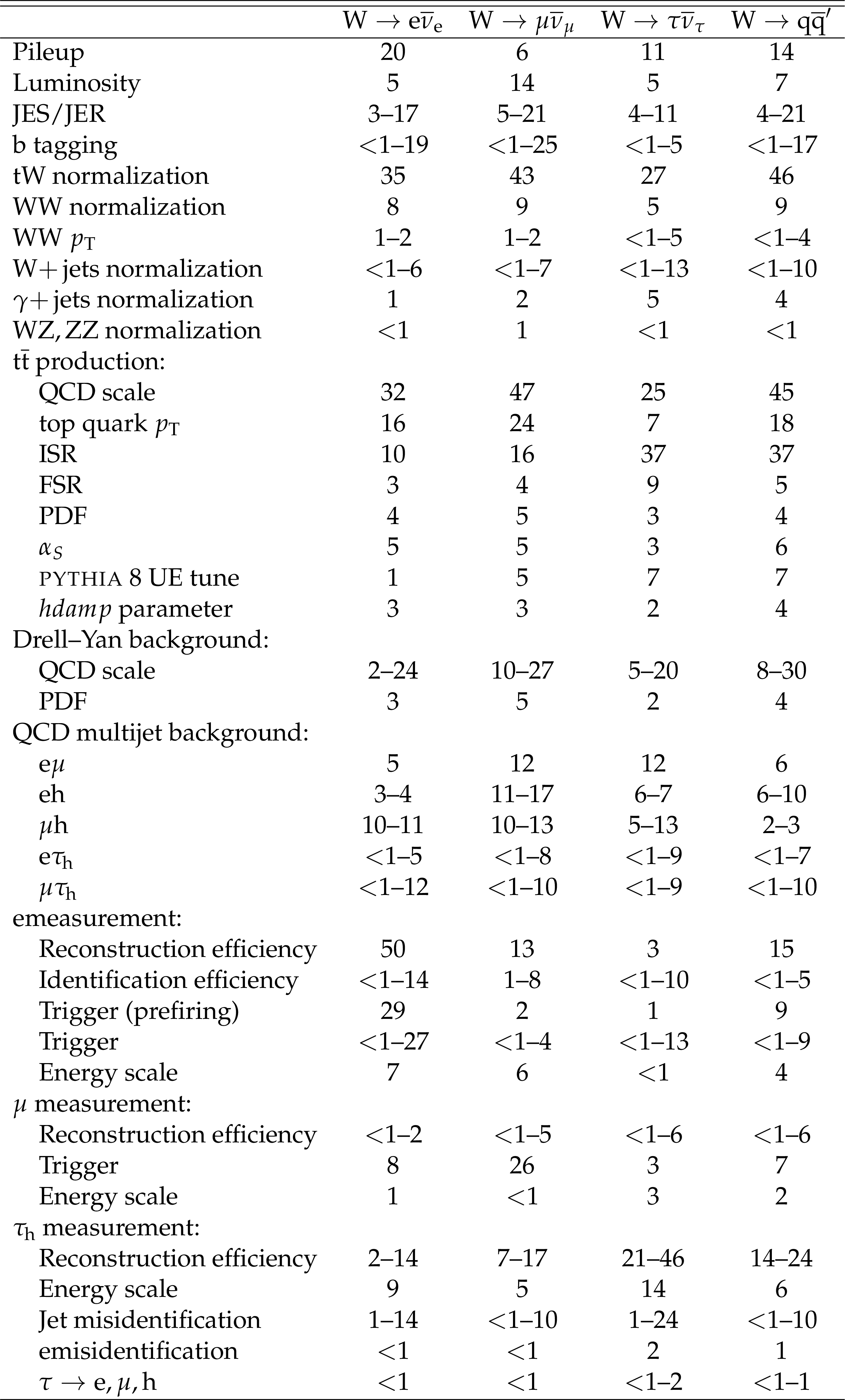
Table 3:
Summary of the impacts of each source of uncertainty (quoted as a percent of the total systematic uncertainty) for each W branching fraction. Whenever multiple NPs impact a common source of systematic uncertainty, each component is varied independently and the range of impacts is given. |

png pdf |
Table 4:
Values of the W boson decay branching fractions measured here compared with the corresponding LEP measurements [8,9]. The lower rows list the average leptonic and inclusive hadronic W branching fractions derived assuming LFU. The first and second uncertainties quoted for each branching fraction correspond to statistical and systematic sources, respectively. |
png pdf |
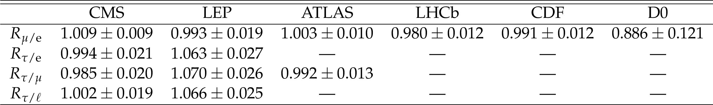
Table 5:
Ratios of different leptonic branching fractions, $R_{\mu /\mathrm{e}} = \mathcal {B}(\mathrm{W} \to \mu \overline{\nu}_{\mu})/\mathcal {B}(\mathrm{W} \to \mathrm{e} \overline{\nu}_{\mathrm{e}})$, $R_{\tau /\mathrm{e}} = \mathcal {B}(\mathrm{W} \to \tau \overline{\nu}_{\tau})/\mathcal {B}(\mathrm{W} \to \mathrm{e} \overline{\nu}_{\mathrm{e}})$, and $R_{\tau /\mu} = \mathcal {B}(\mathrm{W} \to \tau \overline{\nu}_{\tau})/\mathcal {B}(\mathrm{W} \to \mu \overline{\nu}_{\mu})$, measured here compared with the values obtained by other LEP [8], LHC [16,17,13], and Tevatron [14,15] experiments. |

png pdf |
Table 6:
Values of the QCD coupling constant at the W mass, the charm-strange CKM mixing element, and the squared sum of the first two rows of the CKM matrix, derived in this work. |
| Summary |
|
A precise measurement of the three leptonic decay branching fractions of the W boson has been presented, as well as the average leptonic and inclusive hadronic branching fractions assuming lepton flavor universality (LFU). The analysis is based on a data sample of pp collisions at a center-of-mass energy of 13 TeV corresponding to an integrated luminosity of 35.9 fb$^{-1}$ recorded by the CMS experiment. Events with one or two W bosons produced are collected using single-charged-lepton triggers that require at least one prompt electron or muon with large transverse momentum. The extraction of the W boson leptonic branching fractions is performed through a binned maximum likelihood fit of events split into multiple categories defined based on the multiplicity and flavor of reconstructed leptons, the number of jets, and the number of jets identified as originating from the hadronization of b quarks. The measured branching fractions for the decay of the W boson into electrons, muons, tau leptons, and hadrons are (10.83 $\pm$ 0.10)%, (10.94 $\pm$ 0.08)%, (10.77 $\pm$ 0.21)%, and (67.46 $\pm$ 0.28)%, respectively. These results are consistent with the LFU hypothesis for the weak interaction, and are more precise than previous measurements based on data collected by the LEP experiments. Fitting the data assuming LFU provides values of (10.89 $\pm$ 0.08)% and (67.32 $\pm$ 0.23)%, respectively, for the average leptonic and inclusive hadronic branching fractions of the W boson. The comparison of the ratio of hadronic-to-leptonic branching fractions to the theoretical prediction is used to derive other standard model quantities. A value of the strong coupling constant at the W boson mass scale of ${\alpha_S}(m^{2}_\mathrm{W}) = $ 0.095 $\pm$ 0.033 is obtained which, although not competitive compared with the current world average, confirms the usefulness of the W boson decays to constrain this fundamental standard model parameter at future colliders. Using the world average value of ${\alpha_S}(m^{2}_\mathrm{W})$, the sum of the square of the elements in the first two rows of the Cabibbo-Kobayashi-Maskawa (CKM) matrix is $\sum_{ij}|V_{{ij}}|^{2} = $ 1.984 $\pm$ 0.021, providing a precise check of CKM unitarity. From this sum and using the world-average values of the other relevant CKM matrix elements, a value of $|V_{{\mathrm{c}\mathrm{s}}}| = $ 0.967 $\pm$ 0.011 is determined, which is as precise as the current $|V_{{\mathrm{c}\mathrm{s}}}| = $ 0.987 $\pm$ 0.011 result obtained from direct D meson decay data. |
| References | ||||
| 1 | BaBar Collaboration | Evidence for an excess of $ \bar{\mathrm{B}} \to \mathrm{D}^{(*)} \tau^-\bar{\nu}_\tau $ decays | PRL 109 (2012) 101802 | 1205.5442 |
| 2 | BaBar Collaboration | Measurement of an excess of $ \bar{B} \to D^{(*)}\tau^- \bar{\nu}_\tau $ decays and implications for charged Higgs bosons | PRD 88 (2013) 072012 | 1303.0571 |
| 3 | LHCb Collaboration | Measurement of the ratio of branching fractions $ \mathcal{B}(\bar{\mathrm{B}}^0 \to \mathrm{D}^{*+}\tau^{-}\bar{\nu}_{\tau})/\mathcal{B}(\bar{\mathrm{B}}^0 \to \mathrm{D}^{*+}\mu^{-}\bar{\nu}_{\mu}) $ | PRL 115 (2015) 111803 | 1506.08614 |
| 4 | Belle Collaboration | Measurement of the branching ratio of $ \bar{B}^0 \to D^{*+} \tau^- \bar{\nu}_{\tau} $ relative to $ \bar{B}^0 \to D^{*+} \ell^- \bar{\nu}_{\ell} $ decays with a semileptonic tagging method | PRD 94 (2016) 072007 | 1607.07923 |
| 5 | LHCb Collaboration | Measurement of the ratio of branching fractions $ \mathcal{B}(\mathrm{B}_\mathrm{c}^+ \to \mathrm{J}/\psi\tau^+\nu_\tau) $/$ \mathcal{B}(\mathrm{B}_\mathrm{c}^+ \to \mathrm{J}/\psi\mu^+\nu_\mu) $ | PRL 120 (2018) 121801 | 1711.05623 |
| 6 | LHCb Collaboration | Search for lepton-universality violation in $\mathrm{B ^+\to K ^+\ell^+\ell^-} $ decays | PRL 122 (2019) 191801 | 1903.09252 |
| 7 | LHCb Collaboration | Test of lepton universality in beauty-quark decays | 2021 | 2103.11769 |
| 8 | ALEPH, DELPHI, L3, OPAL, LEP Electroweak Collaboration | Electroweak measurements in electron-positron collisions at W-boson-pair energies at LEP | PR 532 (2013) 119 | 1302.3415 |
| 9 | Particle Data Group, P. A. Zyla et al. | Review of particle physics | Prog. Theor. Exp. Phys. 2020 (2020) 083C01 | |
| 10 | A. Denner | Techniques for calculation of electroweak radiative corrections at the one loop level and results for W physics at LEP-200 | Fortsch. Phys. 41 (1993) 307 | 0709.1075 |
| 11 | B. A. Kniehl, F. Madricardo, and M. Steinhauser | Gauge independent W boson partial decay widths | PRD 62 (2000) 073010 | hep-ph/0005060 |
| 12 | D. d'Enterria and V. Jacobsen | Improved strong coupling determinations from hadronic decays of electroweak bosons at N$ ^3 $LO accuracy | 2020. Submitted to PLB | 2005.04545 |
| 13 | ATLAS Collaboration | Test of the universality of $ \tau $ and $ \mu $ lepton couplings in W-boson decays from $ \mathrm{t\bar{t}} $ events with the ATLAS detector | NP 17 (2021) 813 | 2007.14040 |
| 14 | D0 Collaboration | W and Z boson production in $ {{\mathrm{p}}}\bar{{\mathrm{p}}} $ collisions at $ \sqrt{s} = $ 1.8 TeV | PRL 75 (1995) 1456 | hep-ex/9505013 |
| 15 | CDF Collaboration | Measurements of inclusive W and Z cross sections in $ {{\mathrm{p}}}\bar{{\mathrm{p}}} $ collisions at $ \sqrt{s} = $ 1.96 TeV | JPG 34 (2007) 2457 | hep-ex/0508029 |
| 16 | ATLAS Collaboration | Precision measurement and interpretation of inclusive W$ ^+ $, W$ ^- $ and Z/$ \gamma^* $ production cross sections with the ATLAS detector | EPJC 77 (2017) 367 | 1612.03016 |
| 17 | LHCb Collaboration | Measurement of forward W$ \to $e$ \nu $ production in pp collisions at $ \sqrt{s}= $ 8 TeV | JHEP 10 (2016) 030 | 1608.01484 |
| 18 | P. A. Baikov, K. G. Chetyrkin, and J. H. Kuhn | Order $ \alpha_s^4 $ QCD corrections to Z and tau decays | PRL 101 (2008) 012002 | 0801.1821 |
| 19 | D. Kara | Corrections of order $ \alpha \alpha_s $ to W boson decays | NPB 877 (2013) 683 | 1307.7190 |
| 20 | D. d'Enterria and M. Srebre | $ \alpha_s $ and $ V_{\rm cs} $ determination, and CKM unitarity test, from W decays at NNLO | PLB 763 (2016) 465 | 1603.06501 |
| 21 | CMS Collaboration | Precision luminosity measurement in proton-proton collisions at $ \sqrt{s} = $ 13 TeV in 2015 and 2016 at CMS | EPJC 81 (2021) 800 | CMS-LUM-17-003 2104.01927 |
| 22 | CMS Collaboration | The CMS experiment at the CERN LHC | JINST 3 (2008) S08004 | CMS-00-001 |
| 23 | S. Alioli, P. Nason, C. Oleari, and E. Re | A general framework for implementing NLO calculations in shower Monte Carlo programs: the POWHEG BOX | JHEP 06 (2010) 043 | 1002.2581 |
| 24 | A. Kardos, P. Nason, and C. Oleari | Three-jet production in POWHEG | JHEP 04 (2014) 043 | 1402.4001 |
| 25 | S. Frixione and B. R. Webber | Matching NLO QCD computations and parton shower simulations | JHEP 06 (2002) 029 | hep-ph/0204244 |
| 26 | P. Nason | A new method for combining NLO QCD with shower Monte Carlo algorithm | JHEP 11 (2004) 040 | hep-ph/0409146 |
| 27 | E. Re | Single-top Wt-channel production matched with parton showers using the POWHEG method | EPJC 71 (2011) 1547 | 1009.2450 |
| 28 | J. Alwall et al. | MadGraph 5: going beyond | JHEP 06 (2011) 128 | 1106.0522 |
| 29 | J. Alwall et al. | The automated computation of tree-level and next-to-leading order differential cross sections, and their matching to parton shower simulations | JHEP 07 (2014) 079 | 1405.0301 |
| 30 | S. Frixione, P. Nason, and C. Oleari | Matching NLO QCD computations with parton shower simulations: the POWHEG method | JHEP 11 (2007) 070 | 0709.2092 |
| 31 | T. Sjostrand et al. | An introduction to PYTHIA 8.2 | CPC 191 (2015) 159 | 1410.3012 |
| 32 | P. Skands, S. Carrazza, and J. Rojo | Tuning PYTHIA 8.1: the Monash 2013 tune | EPJC 74 (2014) 3024 | 1404.5630 |
| 33 | CMS Collaboration | Event generator tunes obtained from underlying event and multiparton scattering measurements | EPJC 76 (2016) 155 | CMS-GEN-14-001 1512.00815 |
| 34 | CMS Collaboration | Investigations of the impact of the parton shower tuning in PYTHIA 8 in the modelling of $ \mathrm{t\overline{t}} $ at $ \sqrt{s}= $ 8 and 13 TeV | CMS-PAS-TOP-16-021 | CMS-PAS-TOP-16-021 |
| 35 | GEANT4 Collaboration | GEANT4--a simulation toolkit | NIMA 506 (2003) 250 | |
| 36 | CMS Collaboration | Pileup mitigation at CMS in 13 TeV data | JINST 15 (2020) P09018 | CMS-JME-18-001 2003.00503 |
| 37 | CMS Collaboration | Performance of the CMS Level-1 trigger in proton-proton collisions at $ \sqrt{s} = $ 13 TeV | JINST 15 (2020) P10017 | CMS-TRG-17-001 2006.10165 |
| 38 | CMS Collaboration | The CMS trigger system | JINST 12 (2017) P01020 | CMS-TRG-12-001 1609.02366 |
| 39 | CMS Collaboration | Particle-flow reconstruction and global event description with the CMS detector | JINST 12 (2017) P10003 | CMS-PRF-14-001 1706.04965 |
| 40 | M. Cacciari, G. P. Salam, and G. Soyez | The anti-$ {k_{\mathrm{T}}} $ jet clustering algorithm | JHEP 04 (2008) 063 | 0802.1189 |
| 41 | M. Cacciari, G. P. Salam, and G. Soyez | FastJet user manual | EPJC 72 (2012) 1896 | 1111.6097 |
| 42 | CMS Collaboration | Description and performance of track and primary-vertex reconstruction with the CMS tracker | JINST 9 (2014) P10009 | CMS-TRK-11-001 1405.6569 |
| 43 | S. Baffioni et al. | Electron reconstruction in CMS | EPJC 49 (2007) 1099 | |
| 44 | CMS Collaboration | Performance of electron reconstruction and selection with the CMS detector in proton-proton collisions at $ \sqrt{s} = $ 8 TeV | JINST 10 (2015) P06005 | CMS-EGM-13-001 1502.02701 |
| 45 | CMS Collaboration | Performance of CMS muon reconstruction in pp collision events at $ \sqrt{s}= $ 7 TeV | JINST 7 (2012) P10002 | CMS-MUO-10-004 1206.4071 |
| 46 | CMS Collaboration | Performance of the CMS muon detector and muon reconstruction with proton-proton collisions at $ \sqrt{s}= $ 13 TeV | JINST 13 (2018) P06015 | CMS-MUO-16-001 1804.04528 |
| 47 | CMS Collaboration | Performance of reconstruction and identification of $ \tau $ leptons decaying to hadrons and $ \nu_\tau $ in pp collisions at $ \sqrt{s}= $ 13 TeV | JINST 13 (2018) P10005 | CMS-TAU-16-003 1809.02816 |
| 48 | CMS Collaboration | Determination of jet energy calibration and transverse momentum resolution in CMS | JINST 6 (2011) 11002 | CMS-JME-10-011 1107.4277 |
| 49 | CMS Collaboration | Identification of heavy-flavour jets with the CMS detector in pp collisions at 13 TeV | JINST 13 (2018) P05011 | CMS-BTV-16-002 1712.07158 |
| 50 | B. Pollack, S. Bhattacharya, and M. Schmitt | Bayesian blocks in high energy physics: Better binning made easy! | 2017 | 1708.00810 |
| 51 | J. S. Conway | Incorporating nuisance parameters in likelihoods for multisource spectra | in Proceedings, PHYSTAT 2011 Workshop on Statistical Issues Related to Discovery Claims in Search Experiments and Unfolding, CERN 2011 | 1103.0354 |
| 52 | CMS Collaboration | Measurement of the inelastic proton-proton cross section at $ \sqrt{s}= $ 13 TeV | JHEP 07 (2018) 161 | CMS-FSQ-15-005 1802.02613 |
| 53 | CMS Collaboration | Measurement of the production cross section for single top quarks in association with W bosons in proton-proton collisions at $ \sqrt{s}= $ 13 TeV | JHEP 10 (2018) 117 | CMS-TOP-17-018 1805.07399 |
| 54 | ATLAS Collaboration | Measurement of the cross section for isolated-photon plus jet production in pp collisions at $ \sqrt s= $ 13 TeV using the ATLAS detector | PLB 780 (2018) 578 | 1801.00112 |
| 55 | CMS Collaboration | Measurements of the pp $ \to $ WZ inclusive and differential production cross section and constraints on charged anomalous triple gauge couplings at $ \sqrt{s} = $ 13 TeV | JHEP 04 (2019) 122 | CMS-SMP-18-002 1901.03428 |
| 56 | CMS Collaboration | Measurements of pp $ \to $ ZZ production cross sections and constraints on anomalous triple gauge couplings at $ \sqrt{s} = $ 13TeV | EPJC 81 (2021), no. 3, 200 | CMS-SMP-19-001 2009.01186 |
| 57 | CMS Collaboration | Measurements of inclusive W and Z cross sections in pp collisions at $ \sqrt{s}= $ 7 TeV | JHEP 01 (2011) 080 | CMS-EWK-10-002 1012.2466 |
| 58 | CMS Collaboration | Jet energy scale and resolution in the CMS experiment in pp collisions at 8 TeV | JINST 12 (2017) P02014 | CMS-JME-13-004 1607.03663 |
| 59 | CMS Collaboration | Extraction and validation of a new set of CMS PYTHIA8 tunes from underlying-event measurements | EPJC 80 (2020) 4 | CMS-GEN-17-001 1903.12179 |
| 60 | CMS Collaboration | Measurement of the top quark polarization and $ \mathrm{t\bar{t}} $ spin correlations using dilepton final states in proton-proton collisions at $ \sqrt{s} = $ 13 TeV | PRD 100 (2019) 072002 | CMS-TOP-18-006 1907.03729 |
| 61 | CMS Collaboration | Measurement of normalized differential $ \mathrm{t}\overline{\mathrm{t}} $ cross sections in the dilepton channel from pp collisions at $ \sqrt{s}= $ 13 TeV | JHEP 04 (2018) 060 | CMS-TOP-16-007 1708.07638 |
| 62 | CMS Collaboration | Measurement of differential cross sections for top quark pair production using the lepton+jets final state in proton-proton collisions at 13 TeV | PRD 95 (2017) 092001 | CMS-TOP-16-008 1610.04191 |
| 63 | M. Grazzini, S. Kallweit, D. Rathlev, and M. Wiesemann | Transverse-momentum resummation for vector-boson pair production at NNLL+NNLO | JHEP 08 (2015) 154 | 1507.02565 |
| 64 | P. Meade, H. Ramani, and M. Zeng | Transverse momentum resummation effects in W$ ^+ $W$ ^- $ measurements | PRD 90 (2014) 114006 | 1407.4481 |
| 65 | D. V. Hinkley | On the ratio of two correlated normal random variables | Biometrika 56 (1969) 635 | |
| 66 | FCC Collaboration | FCC-ee: The lepton collider: Future Circular Collider conceptual design report volume 2 | EPJST 228 (2019) 261 | |
| 67 | CMS Collaboration | HEPData record for this analysis | link | |
|
|
Compact Muon Solenoid LHC, CERN |
|

|

|

|

|

|