

Compact Muon Solenoid
LHC, CERN
| CMS-B2G-20-009 ; CERN-EP-2022-152 | ||
| Search for new heavy resonances decaying to WW, WZ, ZZ, WH, or ZH boson pairs in the all-jets final state in proton-proton collisions at $ \sqrt{s}= $ 13 TeV | ||
| CMS Collaboration | ||
| 30 September 2022 | ||
| Phys. Lett. B 844 (2023) 137813 | ||
| Abstract: A search for new heavy resonances decaying to WW, WZ, ZZ, WH, or ZH boson pairs in the all-jets final state is presented. The analysis is based on proton-proton collision data recorded by the CMS detector in 2016-2018 at a centre-of-mass energy of 13 TeV at the CERN LHC, corresponding to an integrated luminosity of 138 fb$^{-1}$. The search is sensitive to resonances with masses above 1.3 TeV, decaying to bosons that are highly Lorentz-boosted such that each of the bosons forms a single large-radius jet. Machine learning techniques are employed to identify such jets. No significant excess over the estimated standard model background is observed. A maximum local significance of 3.6 standard deviations, corresponding to a global significance of 2.3 standard deviations, is observed at masses of 2.1 and 2.9 TeV. In a heavy vector triplet model, spin-1 Z' and W' resonances with masses below 4.8 TeV are excluded at the 95% confidence level (CL). These limits are the most stringent to date. In a bulk graviton model, spin-2 gravitons and spin-0 radions with masses below 1.4 and 2.7 TeV, respectively, are excluded at 95% CL. Production of heavy resonances through vector boson fusion is constrained with upper cross section limits at 95% CL as low as 0.1 fb. | ||
| Links: e-print arXiv:2210.00043 [hep-ex] (PDF) ; CDS record ; inSPIRE record ; HepData record ; Physics Briefing ; CADI line (restricted) ; | ||
| Figures & Tables | Summary | Additional Figures | References | CMS Publications |
|---|
| Figures | |

png pdf |
Figure 1:
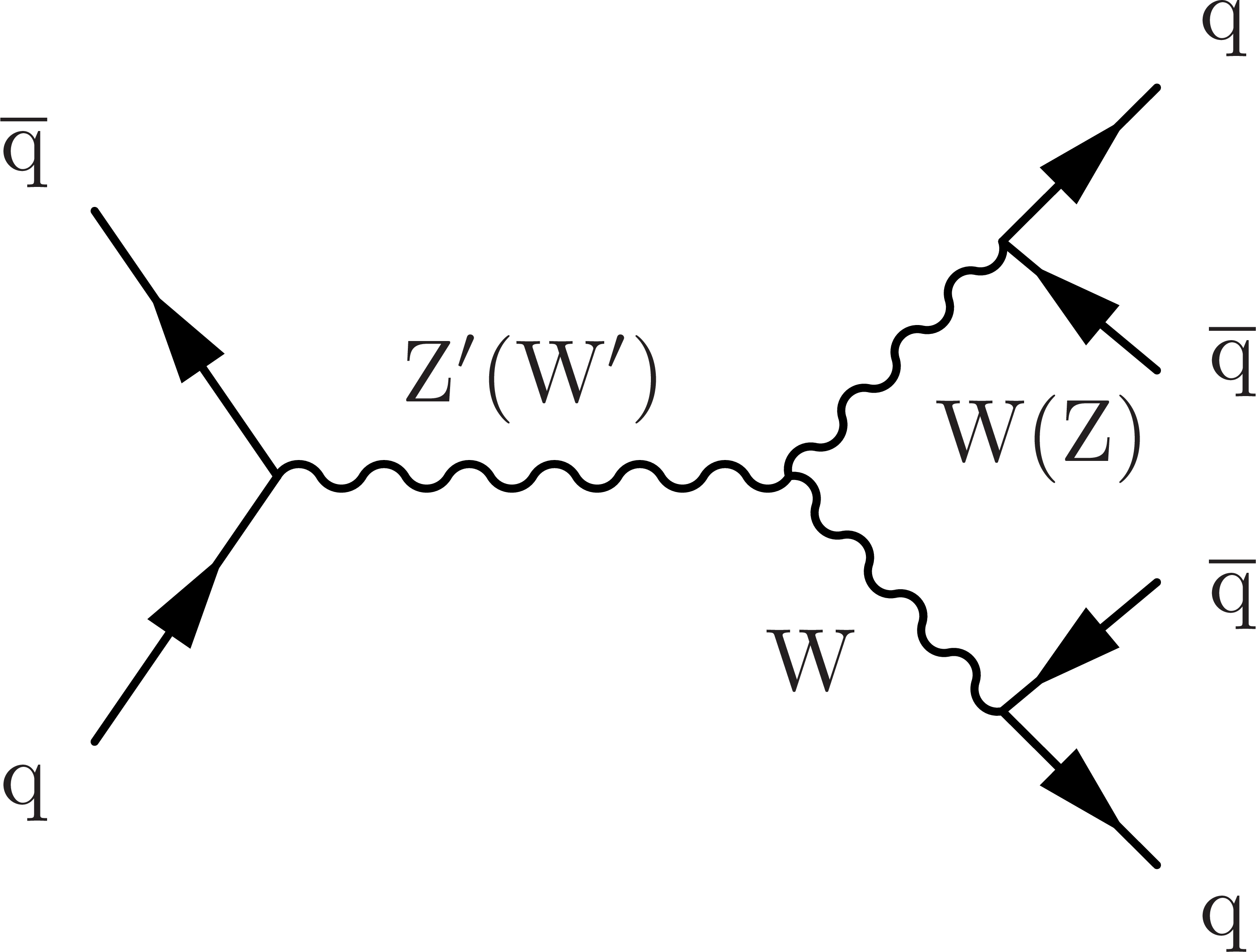
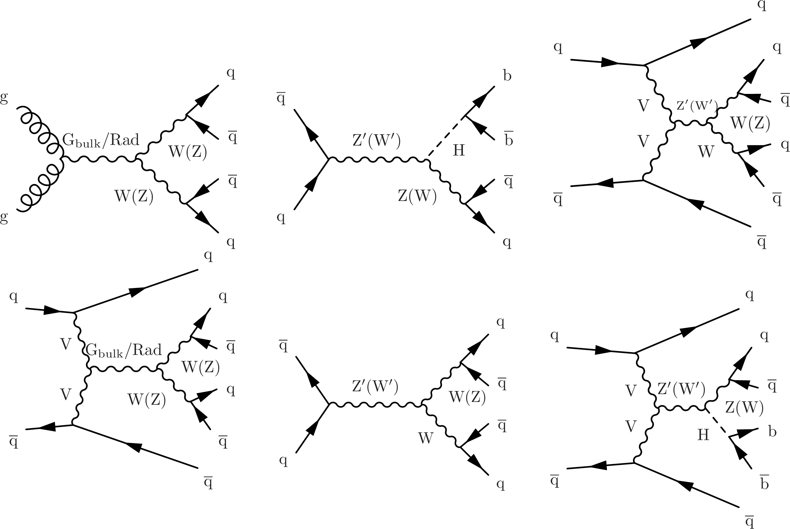
Feynman diagrams of the signal processes ggF or DY produced (upper) and VBF produced (lower): (left) graviton or radion decaying to WW or ZZ; (center) Z' and W' decaying to ZH and WH, respectively; (right) Z' and W' decaying to WW and WZ, respectively. |

png pdf |
Figure 1-a:
Example Feynman diagram of signal process: DY produced graviton or radion decaying to WW or ZZ. |

png pdf |
Figure 1-b:
Example Feynman diagram of signal process: DY produced Z' and W' decaying to ZH and WH, respectively. |
png pdf |
Figure 1-c:
Example Feynman diagram of signal process: DY produced Z' and W' decaying to WW and WZ, respectively. |
png pdf |
Figure 1-d:
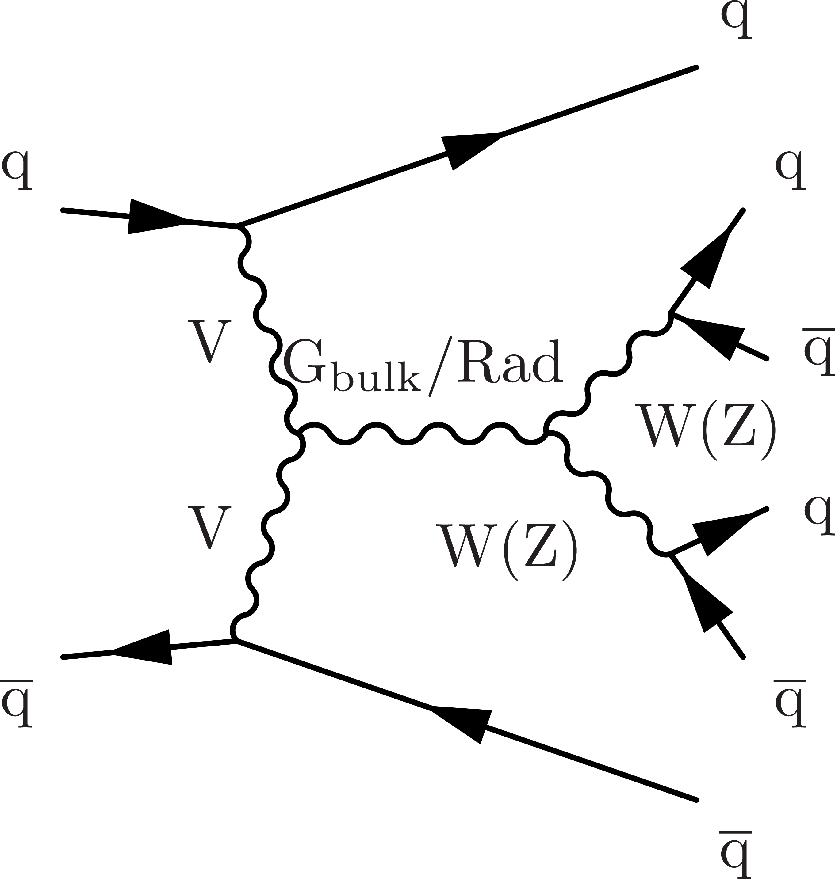
Example Feynman diagram of signal process: VBF produced graviton or radion decaying to WW or ZZ. |

png pdf |
Figure 1-e:
Example Feynman diagram of signal process: VBF produced Z' and W' decaying to ZH and WH, respectively. |

png pdf |
Figure 1-f:
Example Feynman diagram of signal process: VBF produced Z' and W' decaying to WW and WZ, respectively. |

png pdf |
Figure 2:
Distributions of $ m_\mathrm{jj}^{ \mathrm{AK8} } $ (left) and $ m_\text{jet1}^{ \mathrm{AK8} } $ (right) in the nominal QCD multijet simulation using PYTHIA 8 (black markers) and three-dimensional templates (black solid line) in the DY/ggF VH HPHP category. Superimposed are the normalized up and down variations of five alternative shapes corresponding to shape nuisance parameters in the fit model. Each of the variations has a characteristic dependence on $ m_\text{jet}^{ \mathrm{AK8} } $ to allow the necessary flexibility in the fit for the template to adapt to the data. We also allow an overall variation of the rate in the fit. |

png pdf |
Figure 2-a:
Distribution of $ m_\mathrm{jj}^{ \mathrm{AK8} } $ in the nominal QCD multijet simulation using PYTHIA 8 (black markers) and three-dimensional templates (black solid line) in the DY/ggF VH HPHP category. Superimposed are the normalized up and down variations of five alternative shapes corresponding to shape nuisance parameters in the fit model. Each of the variations has a characteristic dependence on $ m_\text{jet}^{ \mathrm{AK8} } $ to allow the necessary flexibility in the fit for the template to adapt to the data. We also allow an overall variation of the rate in the fit. |

png pdf |
Figure 2-b:
Distribution of $ m_\text{jet1}^{ \mathrm{AK8} } $ in the nominal QCD multijet simulation using PYTHIA 8 (black markers) and three-dimensional templates (black solid line) in the DY/ggF VH HPHP category. Superimposed are the normalized up and down variations of five alternative shapes corresponding to shape nuisance parameters in the fit model. Each of the variations has a characteristic dependence on $ m_\text{jet}^{ \mathrm{AK8} } $ to allow the necessary flexibility in the fit for the template to adapt to the data. We also allow an overall variation of the rate in the fit. |

png pdf |
Figure 3:
Comparison between the background post-fit and the data distributions of $ m_\mathrm{jj}^{ \mathrm{AK8} } $ (left) and $ m_\text{jet1}^{ \mathrm{AK8} } $ (right) in the DY/ggF VH HPHP category. The background shape uncertainty is shown as a gray shaded band around the result of the maximum likelihood fit to the data under the background-only assumption (gray solid line), and the statistical uncertainties in the data are represented as vertical bars. The various background components contributing to the total background fit are also shown with different line colors. An example of a signal distribution is overlaid, where the number of expected events is scaled by an arbitrary normalization factor of 20. Shown below each mass plot is the difference between the data and the fit divided by the statistical uncertainty in the data; the uncertainty bar represents the statistical uncertainty only. The total uncertainty in the background estimate fitted to the data divided by the statistical uncertainty in the data is shown as a band. |

png pdf |
Figure 3-a:
Comparison between the background post-fit and the data distributions of $ m_\mathrm{jj}^{ \mathrm{AK8} } $ in the DY/ggF VH HPHP category. The background shape uncertainty is shown as a gray shaded band around the result of the maximum likelihood fit to the data under the background-only assumption (gray solid line), and the statistical uncertainties in the data are represented as vertical bars. The various background components contributing to the total background fit are also shown with different line colors. An example of a signal distribution is overlaid, where the number of expected events is scaled by an arbitrary normalization factor of 20. Shown below the plot is the difference between the data and the fit divided by the statistical uncertainty in the data; the uncertainty bar represents the statistical uncertainty only. The total uncertainty in the background estimate fitted to the data divided by the statistical uncertainty in the data is shown as a band. |

png pdf |
Figure 3-b:
Comparison between the background post-fit and the data distributions of $ m_\text{jet1}^{ \mathrm{AK8} } $ in the DY/ggF VH HPHP category. The background shape uncertainty is shown as a gray shaded band around the result of the maximum likelihood fit to the data under the background-only assumption (gray solid line), and the statistical uncertainties in the data are represented as vertical bars. The various background components contributing to the total background fit are also shown with different line colors. An example of a signal distribution is overlaid, where the number of expected events is scaled by an arbitrary normalization factor of 20. Shown below the plot is the difference between the data and the fit divided by the statistical uncertainty in the data; the uncertainty bar represents the statistical uncertainty only. The total uncertainty in the background estimate fitted to the data divided by the statistical uncertainty in the data is shown as a band. |

png pdf |
Figure 4:
Projections of the data and background post-fit distributions onto the $ m_\mathrm{jj}^{ \mathrm{AK8} } $ dimension in regions enriched in background ($ m_\text{jet1}^{\mathrm{AK8}} < $ 65 or $ > $140 GeV, and $ m_\text{jet2}^{\mathrm{AK8}} < $ 65 or $ > $140 GeV), for the HPHP VH (left) and VV (right) DY/ggF categories. The background shape uncertainty is shown as a gray shaded band around the result of the maximum likelihood fit to the data under the background-only assumption (gray solid line), and the statistical uncertainties in the data are shown as vertical bars. The various background components contributing to the total background fit are also shown with different line colors. Shown below each mass plot is the difference between the data and the fit divided by the statistical uncertainty in the data; the uncertainty bar represents the statistical uncertainty only. The total uncertainty in the background estimate fitted to the data divided by the statistical uncertainty in the data is shown as a band. |

png pdf |
Figure 4-a:
Projection of the data and background post-fit distributions onto the $ m_\mathrm{jj}^{ \mathrm{AK8} } $ dimension in regions enriched in background ($ m_\text{jet1}^{\mathrm{AK8}} < $ 65 or $ > $140 GeV, and $ m_\text{jet2}^{\mathrm{AK8}} < $ 65 or $ > $140 GeV), for the HPHP VH DY/ggF category. The background shape uncertainty is shown as a gray shaded band around the result of the maximum likelihood fit to the data under the background-only assumption (gray solid line), and the statistical uncertainties in the data are shown as vertical bars. The various background components contributing to the total background fit are also shown with different line colors. Shown below the plot is the difference between the data and the fit divided by the statistical uncertainty in the data; the uncertainty bar represents the statistical uncertainty only. The total uncertainty in the background estimate fitted to the data divided by the statistical uncertainty in the data is shown as a band. |

png pdf |
Figure 4-b:
Projection of the data and background post-fit distributions onto the $ m_\mathrm{jj}^{ \mathrm{AK8} } $ dimension in regions enriched in background ($ m_\text{jet1}^{\mathrm{AK8}} < $ 65 or $ > $140 GeV, and $ m_\text{jet2}^{\mathrm{AK8}} < $ 65 or $ > $140 GeV), for the HPHP VV DY/ggF category. The background shape uncertainty is shown as a gray shaded band around the result of the maximum likelihood fit to the data under the background-only assumption (gray solid line), and the statistical uncertainties in the data are shown as vertical bars. The various background components contributing to the total background fit are also shown with different line colors. Shown below the plot is the difference between the data and the fit divided by the statistical uncertainty in the data; the uncertainty bar represents the statistical uncertainty only. The total uncertainty in the background estimate fitted to the data divided by the statistical uncertainty in the data is shown as a band. |

png pdf |
Figure 5:
Projections of data and background post-fit distributions onto the $ m_\mathrm{jj}^{ \mathrm{AK8} } $ dimension in regions enriched in signal from DY/ggF VV ( 65 $ < m_\text{jet1}^{\mathrm{AK8}} < $ 105 GeV, 65 $ < m_\text{jet2}^{\mathrm{AK8}} < $ 105 GeV) for the HPHP VH (left) and VV (right) DY/ggF categories. The background shape uncertainty is shown as a gray shaded band around the result of the maximum likelihood fit to the data under the background-only assumption (gray solid line), and the statistical uncertainties in the data are shown as vertical bars. The various background components contributing to the total background fit are also shown with different line colors. An example of a signal distribution is overlaid. Shown below each mass plot is the difference between the data and the fit divided by the statistical uncertainty in the data; the uncertainty bar represents the statistical uncertainty only. The total uncertainty in the background estimate fitted to the data divided by the statistical uncertainty in the data is shown as a band. |

png pdf |
Figure 5-a:
Projection of data and background post-fit distributions onto the $ m_\mathrm{jj}^{ \mathrm{AK8} } $ dimension in regions enriched in signal from DY/ggF VV ( 65 $ < m_\text{jet1}^{\mathrm{AK8}} < $ 105 GeV, 65 $ < m_\text{jet2}^{\mathrm{AK8}} < $ 105 GeV) for the HPHP VH DY/ggF categories. The background shape uncertainty is shown as a gray shaded band around the result of the maximum likelihood fit to the data under the background-only assumption (gray solid line), and the statistical uncertainties in the data are shown as vertical bars. The various background components contributing to the total background fit are also shown with different line colors. An example of a signal distribution is overlaid. Shown below the plot is the difference between the data and the fit divided by the statistical uncertainty in the data; the uncertainty bar represents the statistical uncertainty only. The total uncertainty in the background estimate fitted to the data divided by the statistical uncertainty in the data is shown as a band. |

png pdf |
Figure 5-b:
Projection of data and background post-fit distributions onto the $ m_\mathrm{jj}^{ \mathrm{AK8} } $ dimension in regions enriched in signal from DY/ggF VV ( 65 $ < m_\text{jet1}^{\mathrm{AK8}} < $ 105 GeV, 65 $ < m_\text{jet2}^{\mathrm{AK8}} < $ 105 GeV) for the HPHP VV DY/ggF categories. The background shape uncertainty is shown as a gray shaded band around the result of the maximum likelihood fit to the data under the background-only assumption (gray solid line), and the statistical uncertainties in the data are shown as vertical bars. The various background components contributing to the total background fit are also shown with different line colors. An example of a signal distribution is overlaid. Shown below the plot is the difference between the data and the fit divided by the statistical uncertainty in the data; the uncertainty bar represents the statistical uncertainty only. The total uncertainty in the background estimate fitted to the data divided by the statistical uncertainty in the data is shown as a band. |

png pdf |
Figure 6:
Distributions of the difference between the data and the background-only fit divided by the statistical uncertainty in the data. The total uncertainty in the background estimate fitted to data divided by the statistical uncertainty in the data is shown as a band. It should be noted that these two uncertainties are partially correlated. Three projections of the 3D phase space are shown in regions enriched in signal from DY/ggF VV (65 $ < m_\text{jet1}^{\mathrm{AK8}} < $ 105 GeV, 65 $ < m_\text{jet2}^{\mathrm{AK8}} < $ 105 GeV) (upper left), DY/ggF VH (65 $ < m_\text{jet1/2}^{\mathrm{AK8}} < $ 105 GeV, 110 $ < m_\text{jet2/1}^{\mathrm{AK8}} < $ 140 GeV) (upper right) and VBF VV/VH (65 $ < m_\text{jet1}^{\mathrm{AK8}} < $ 140 GeV, 65 $ < m_\text{jet2}^{\mathrm{AK8}} < $ 140 GeV) (lower). Examples of expected signal shapes added to the fit are overlaid, where the number of expected events is scaled by an arbitrary normalization factor stated in the legend. |

png pdf |
Figure 6-a:
Distribution of the difference between the data and the background-only fit divided by the statistical uncertainty in the data. The total uncertainty in the background estimate fitted to data divided by the statistical uncertainty in the data is shown as a band. It should be noted that these two uncertainties are partially correlated. The projection of the 3D phase space is shown in the 65 $ < m_\text{jet1}^{\mathrm{AK8}} < $ 105 GeV, 65 $ < m_\text{jet2}^{\mathrm{AK8}} < $ 105 GeV region. Examples of expected signal shapes added to the fit are overlaid, where the number of expected events is scaled by an arbitrary normalization factor stated in the legend. |

png pdf |
Figure 6-b:
Distribution of the difference between the data and the background-only fit divided by the statistical uncertainty in the data. The total uncertainty in the background estimate fitted to data divided by the statistical uncertainty in the data is shown as a band. It should be noted that these two uncertainties are partially correlated. The projection of the 3D phase space is shown in the DY/ggF VH (65 $ < m_\text{jet1/2}^{\mathrm{AK8}} < $ 105 GeV, 110 $ < m_\text{jet2/1}^{\mathrm{AK8}} < $ 140 GeV region. Examples of expected signal shapes added to the fit are overlaid, where the number of expected events is scaled by an arbitrary normalization factor stated in the legend. |

png pdf |
Figure 6-c:
Distribution of the difference between the data and the background-only fit divided by the statistical uncertainty in the data. The total uncertainty in the background estimate fitted to data divided by the statistical uncertainty in the data is shown as a band. It should be noted that these two uncertainties are partially correlated. The projection of the 3D phase space is shown in the VBF VV/VH (65 $ < m_\text{jet1}^{\mathrm{AK8}} < $ 140 GeV, 65 $ < m_\text{jet2}^{\mathrm{AK8}} < $ 140 GeV region. Examples of expected signal shapes added to the fit are overlaid, where the number of expected events is scaled by an arbitrary normalization factor stated in the legend. |

png pdf |
Figure 7:
Observed and expected 95% CL upper limits on the product of the production cross section ($ \sigma $) and the branching fraction, obtained after combining all categories with 138 fb$^{-1}$ of data at $ \sqrt{s}= $ 13 TeV, for $ \text{Rad}\to\mathrm{V}\mathrm{V} $ (upper left), $ \mathrm{G}_{\text{bulk}}\to\mathrm{V}\mathrm{V} $ (upper right), HVT model B $ \mathrm{V}^\prime\to\mathrm{V}\mathrm{V} $+ VH (lower left), HVT model C $ \mathrm{V}^\prime\to\mathrm{V}\mathrm{V} $+ VH (lower right) signals. For each signal scenario the theoretical prediction and its uncertainty associated with the choice of PDF set is shown. |

png pdf |
Figure 7-a:
Observed and expected 95% CL upper limits on the product of the production cross section ($ \sigma $) and the branching fraction, obtained after combining all categories with 138 fb$^{-1}$ of data at $ \sqrt{s}= $ 13 TeV, for $ \text{Rad}\to\mathrm{V}\mathrm{V} $ signals. The theoretical prediction and its uncertainty associated with the choice of PDF set is shown. |

png pdf |
Figure 7-b:
Observed and expected 95% CL upper limits on the product of the production cross section ($ \sigma $) and the branching fraction, obtained after combining all categories with 138 fb$^{-1}$ of data at $ \sqrt{s}= $ 13 TeV, for $ \mathrm{G}_{\text{bulk}}\to\mathrm{V}\mathrm{V} $ signals. The theoretical prediction and its uncertainty associated with the choice of PDF set is shown. |

png pdf |
Figure 7-c:
Observed and expected 95% CL upper limits on the product of the production cross section ($ \sigma $) and the branching fraction, obtained after combining all categories with 138 fb$^{-1}$ of data at $ \sqrt{s}= $ 13 TeV, for HVT model B $ \mathrm{V}^\prime\to\mathrm{V}\mathrm{V} $+ VH signals. The theoretical prediction and its uncertainty associated with the choice of PDF set is shown. |

png pdf |
Figure 7-d:
Observed and expected 95% CL upper limits on the product of the production cross section ($ \sigma $) and the branching fraction, obtained after combining all categories with 138 fb$^{-1}$ of data at $ \sqrt{s}= $ 13 TeV, for HVT model C $ \mathrm{V}^\prime\to\mathrm{V}\mathrm{V} $+ VH signals. The theoretical prediction and its uncertainty associated with the choice of PDF set is shown. |
| Tables | |

png pdf |
Table 1:
Summary of the event category definitions. The categories are listed from the highest to the lowest sensitivity in each production mode. The percentages correspond to the maximum misidentification rate associated with the high (HP) and low (LP) purity working points. |

png pdf |
Table 2:
Summary of the exclusion limits on the resonance masses for the considered models. The numbers show the lower limit at 95% CL, with the exception of the ones given in parentheses quoting the ranges of exclusion. |
| Summary |
| A search has been presented for resonances with masses above 1.3 TeV that decay to WW, WZ, ZZ, WH, or ZH boson pairs. Each of the two boson decays is clustered into one large-radius jet, yielding a dijet final state from Drell--Yan and gluon fusion production, complemented by two additional jets for vector boson fusion production. The hadronic decays of H, W, and Z bosons are identified using machine learning-based jet taggers that reduce the background from quantum chromodynamics multijet production. No evidence of a departure from the expected background is found. A maximum local significance of 3.6 standard deviations from the standard model prediction, corresponding to a global significance of 2.3 standard deviations, is observed at masses of 2.1 and 2.9 TeV. Upper limits at 95% confidence level on the resonance production cross section are set as a function of the resonance mass. In a heavy vector triplet model, spin-1 Z' and W' resonances with masses below 4.8 TeV are excluded. These limits are the most stringent to date. In a bulk graviton model, spin-2 gravitons and spin-0 radions with masses below 1.4 and 2.7 TeV, respectively, are excluded. Furthermore, the exclusive production of new heavy resonances through the vector boson fusion mode is constrained with upper cross section limits as low as 0.1 fb. |
| Additional Figures | |
png pdf |
Additional Figure 1:
Example Feynman diagrams of signal processes: (top left) $ \mathrm{g} \mathrm{g} $ produced graviton or radion decaying to WW or ZZ; (top center) DY produced $ \mathrm{Z}^{'} $ and $ \mathrm{W^{'}} $ decaying to ZH and WH, respectively; (top right) VBF produced $ \mathrm{Z}^{'} $ and $ \mathrm{W^{'}} $ decaying to WW and WZ, respectively; (bottom left) VBF produced graviton or radion decaying to WW or ZZ; (bottom center) DY produced $ \mathrm{Z}^{'} $ and $ \mathrm{W^{'}} $ decaying to WW and WZ, respectively; (bottom right) VBF produced $ \mathrm{Z}^{'} $ and $ \mathrm{W^{'}} $ decaying to ZH and WH, respectively. The diagrams on the top are shown in the paper as well, and are included here for convenience. |

png pdf |
Additional Figure 1-a:
Example Feynman diagrams of signal processes: (top left) $ \mathrm{g} \mathrm{g} $ produced graviton or radion decaying to WW or ZZ; (top center) DY produced $ \mathrm{Z}^{'} $ and $ \mathrm{W^{'}} $ decaying to ZH and WH, respectively; (top right) VBF produced $ \mathrm{Z}^{'} $ and $ \mathrm{W^{'}} $ decaying to WW and WZ, respectively; (bottom left) VBF produced graviton or radion decaying to WW or ZZ; (bottom center) DY produced $ \mathrm{Z}^{'} $ and $ \mathrm{W^{'}} $ decaying to WW and WZ, respectively; (bottom right) VBF produced $ \mathrm{Z}^{'} $ and $ \mathrm{W^{'}} $ decaying to ZH and WH, respectively. The diagrams on the top are shown in the paper as well, and are included here for convenience. |

png pdf |
Additional Figure 1-b:
Example Feynman diagrams of signal processes: (top left) $ \mathrm{g} \mathrm{g} $ produced graviton or radion decaying to WW or ZZ; (top center) DY produced $ \mathrm{Z}^{'} $ and $ \mathrm{W^{'}} $ decaying to ZH and WH, respectively; (top right) VBF produced $ \mathrm{Z}^{'} $ and $ \mathrm{W^{'}} $ decaying to WW and WZ, respectively; (bottom left) VBF produced graviton or radion decaying to WW or ZZ; (bottom center) DY produced $ \mathrm{Z}^{'} $ and $ \mathrm{W^{'}} $ decaying to WW and WZ, respectively; (bottom right) VBF produced $ \mathrm{Z}^{'} $ and $ \mathrm{W^{'}} $ decaying to ZH and WH, respectively. The diagrams on the top are shown in the paper as well, and are included here for convenience. |

png pdf |
Additional Figure 1-c:
Example Feynman diagrams of signal processes: (top left) $ \mathrm{g} \mathrm{g} $ produced graviton or radion decaying to WW or ZZ; (top center) DY produced $ \mathrm{Z}^{'} $ and $ \mathrm{W^{'}} $ decaying to ZH and WH, respectively; (top right) VBF produced $ \mathrm{Z}^{'} $ and $ \mathrm{W^{'}} $ decaying to WW and WZ, respectively; (bottom left) VBF produced graviton or radion decaying to WW or ZZ; (bottom center) DY produced $ \mathrm{Z}^{'} $ and $ \mathrm{W^{'}} $ decaying to WW and WZ, respectively; (bottom right) VBF produced $ \mathrm{Z}^{'} $ and $ \mathrm{W^{'}} $ decaying to ZH and WH, respectively. The diagrams on the top are shown in the paper as well, and are included here for convenience. |

png pdf |
Additional Figure 1-d:
Example Feynman diagrams of signal processes: (top left) $ \mathrm{g} \mathrm{g} $ produced graviton or radion decaying to WW or ZZ; (top center) DY produced $ \mathrm{Z}^{'} $ and $ \mathrm{W^{'}} $ decaying to ZH and WH, respectively; (top right) VBF produced $ \mathrm{Z}^{'} $ and $ \mathrm{W^{'}} $ decaying to WW and WZ, respectively; (bottom left) VBF produced graviton or radion decaying to WW or ZZ; (bottom center) DY produced $ \mathrm{Z}^{'} $ and $ \mathrm{W^{'}} $ decaying to WW and WZ, respectively; (bottom right) VBF produced $ \mathrm{Z}^{'} $ and $ \mathrm{W^{'}} $ decaying to ZH and WH, respectively. The diagrams on the top are shown in the paper as well, and are included here for convenience. |

png pdf |
Additional Figure 1-e:
Example Feynman diagrams of signal processes: (top left) $ \mathrm{g} \mathrm{g} $ produced graviton or radion decaying to WW or ZZ; (top center) DY produced $ \mathrm{Z}^{'} $ and $ \mathrm{W^{'}} $ decaying to ZH and WH, respectively; (top right) VBF produced $ \mathrm{Z}^{'} $ and $ \mathrm{W^{'}} $ decaying to WW and WZ, respectively; (bottom left) VBF produced graviton or radion decaying to WW or ZZ; (bottom center) DY produced $ \mathrm{Z}^{'} $ and $ \mathrm{W^{'}} $ decaying to WW and WZ, respectively; (bottom right) VBF produced $ \mathrm{Z}^{'} $ and $ \mathrm{W^{'}} $ decaying to ZH and WH, respectively. The diagrams on the top are shown in the paper as well, and are included here for convenience. |

png pdf |
Additional Figure 1-f:
Example Feynman diagrams of signal processes: (top left) $ \mathrm{g} \mathrm{g} $ produced graviton or radion decaying to WW or ZZ; (top center) DY produced $ \mathrm{Z}^{'} $ and $ \mathrm{W^{'}} $ decaying to ZH and WH, respectively; (top right) VBF produced $ \mathrm{Z}^{'} $ and $ \mathrm{W^{'}} $ decaying to WW and WZ, respectively; (bottom left) VBF produced graviton or radion decaying to WW or ZZ; (bottom center) DY produced $ \mathrm{Z}^{'} $ and $ \mathrm{W^{'}} $ decaying to WW and WZ, respectively; (bottom right) VBF produced $ \mathrm{Z}^{'} $ and $ \mathrm{W^{'}} $ decaying to ZH and WH, respectively. The diagrams on the top are shown in the paper as well, and are included here for convenience. |

png pdf |
Additional Figure 2:
Total signal efficiency including all event categories as a function of the resonance mass $M_{\mathrm{X}}$ for all DY/ggF (left) and VBF (right) signal models under consideration. The estimates from MC simulation (markers) are interpolated with a functional form (lines). |

png pdf |
Additional Figure 2-a:
Total signal efficiency including all event categories as a function of the resonance mass $M_{\mathrm{X}}$ for all DY/ggF (left) and VBF (right) signal models under consideration. The estimates from MC simulation (markers) are interpolated with a functional form (lines). |

png pdf |
Additional Figure 2-b:
Total signal efficiency including all event categories as a function of the resonance mass $M_{\mathrm{X}}$ for all DY/ggF (left) and VBF (right) signal models under consideration. The estimates from MC simulation (markers) are interpolated with a functional form (lines). |
png pdf |
Additional Figure 3:
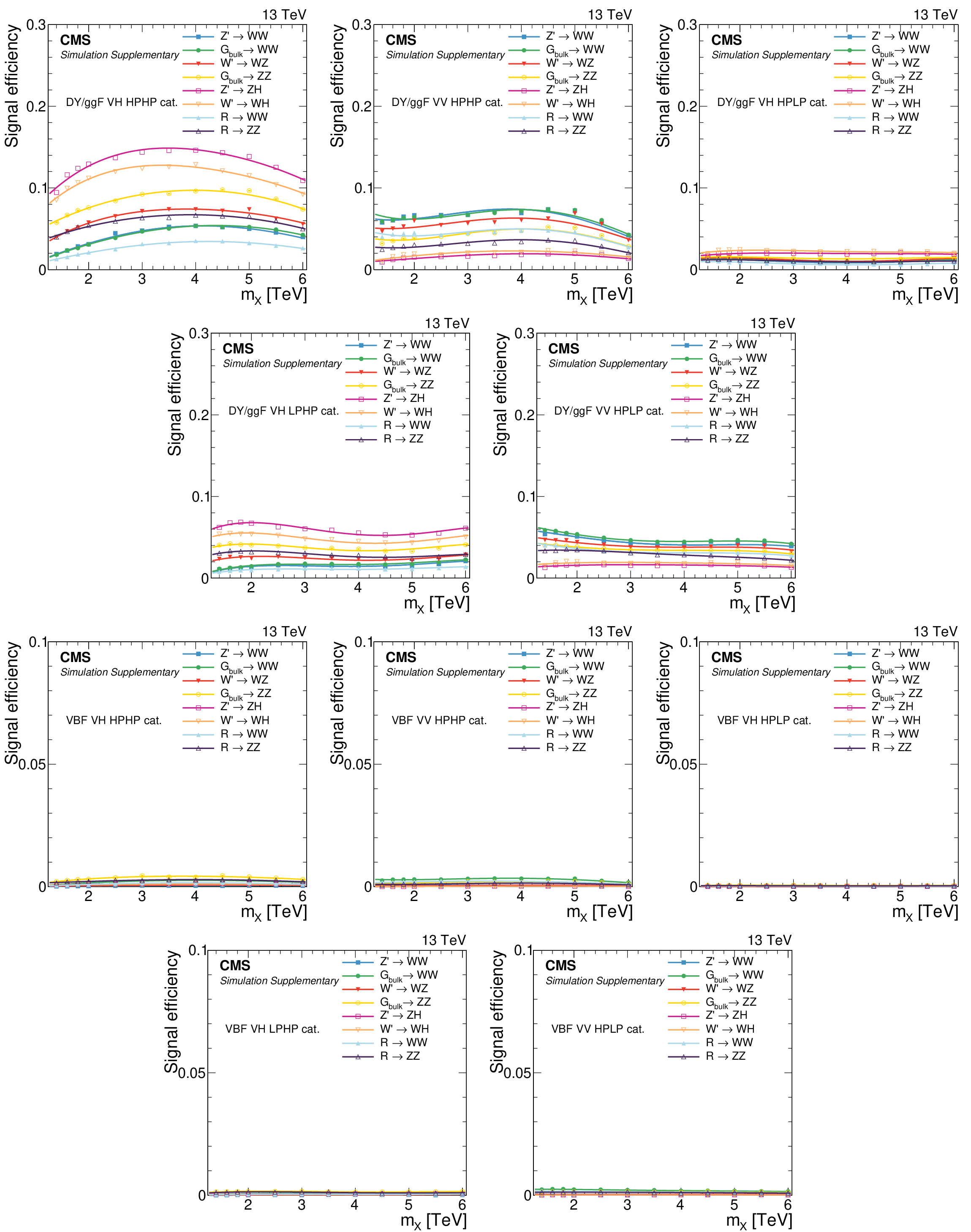
Signal efficiency in each of the categories as a function of the resonance mass $M_{\mathrm{X}}$ for all DY/ggF signal models under consideration. The estimates from MC simulation (markers) are interpolated with a functional form (lines). |

png pdf |
Additional Figure 3-a:
Signal efficiency in each of the categories as a function of the resonance mass $M_{\mathrm{X}}$ for all DY/ggF signal models under consideration. The estimates from MC simulation (markers) are interpolated with a functional form (lines). |

png pdf |
Additional Figure 3-b:
Signal efficiency in each of the categories as a function of the resonance mass $M_{\mathrm{X}}$ for all DY/ggF signal models under consideration. The estimates from MC simulation (markers) are interpolated with a functional form (lines). |

png pdf |
Additional Figure 3-c:
Signal efficiency in each of the categories as a function of the resonance mass $M_{\mathrm{X}}$ for all DY/ggF signal models under consideration. The estimates from MC simulation (markers) are interpolated with a functional form (lines). |

png pdf |
Additional Figure 3-d:
Signal efficiency in each of the categories as a function of the resonance mass $M_{\mathrm{X}}$ for all DY/ggF signal models under consideration. The estimates from MC simulation (markers) are interpolated with a functional form (lines). |

png pdf |
Additional Figure 3-e:
Signal efficiency in each of the categories as a function of the resonance mass $M_{\mathrm{X}}$ for all DY/ggF signal models under consideration. The estimates from MC simulation (markers) are interpolated with a functional form (lines). |

png pdf |
Additional Figure 3-f:
Signal efficiency in each of the categories as a function of the resonance mass $M_{\mathrm{X}}$ for all DY/ggF signal models under consideration. The estimates from MC simulation (markers) are interpolated with a functional form (lines). |

png pdf |
Additional Figure 3-g:
Signal efficiency in each of the categories as a function of the resonance mass $M_{\mathrm{X}}$ for all DY/ggF signal models under consideration. The estimates from MC simulation (markers) are interpolated with a functional form (lines). |

png pdf |
Additional Figure 3-h:
Signal efficiency in each of the categories as a function of the resonance mass $M_{\mathrm{X}}$ for all DY/ggF signal models under consideration. The estimates from MC simulation (markers) are interpolated with a functional form (lines). |
png pdf |
Additional Figure 3-i:
Signal efficiency in each of the categories as a function of the resonance mass $M_{\mathrm{X}}$ for all DY/ggF signal models under consideration. The estimates from MC simulation (markers) are interpolated with a functional form (lines). |

png pdf |
Additional Figure 3-j:
Signal efficiency in each of the categories as a function of the resonance mass $M_{\mathrm{X}}$ for all DY/ggF signal models under consideration. The estimates from MC simulation (markers) are interpolated with a functional form (lines). |

png pdf |
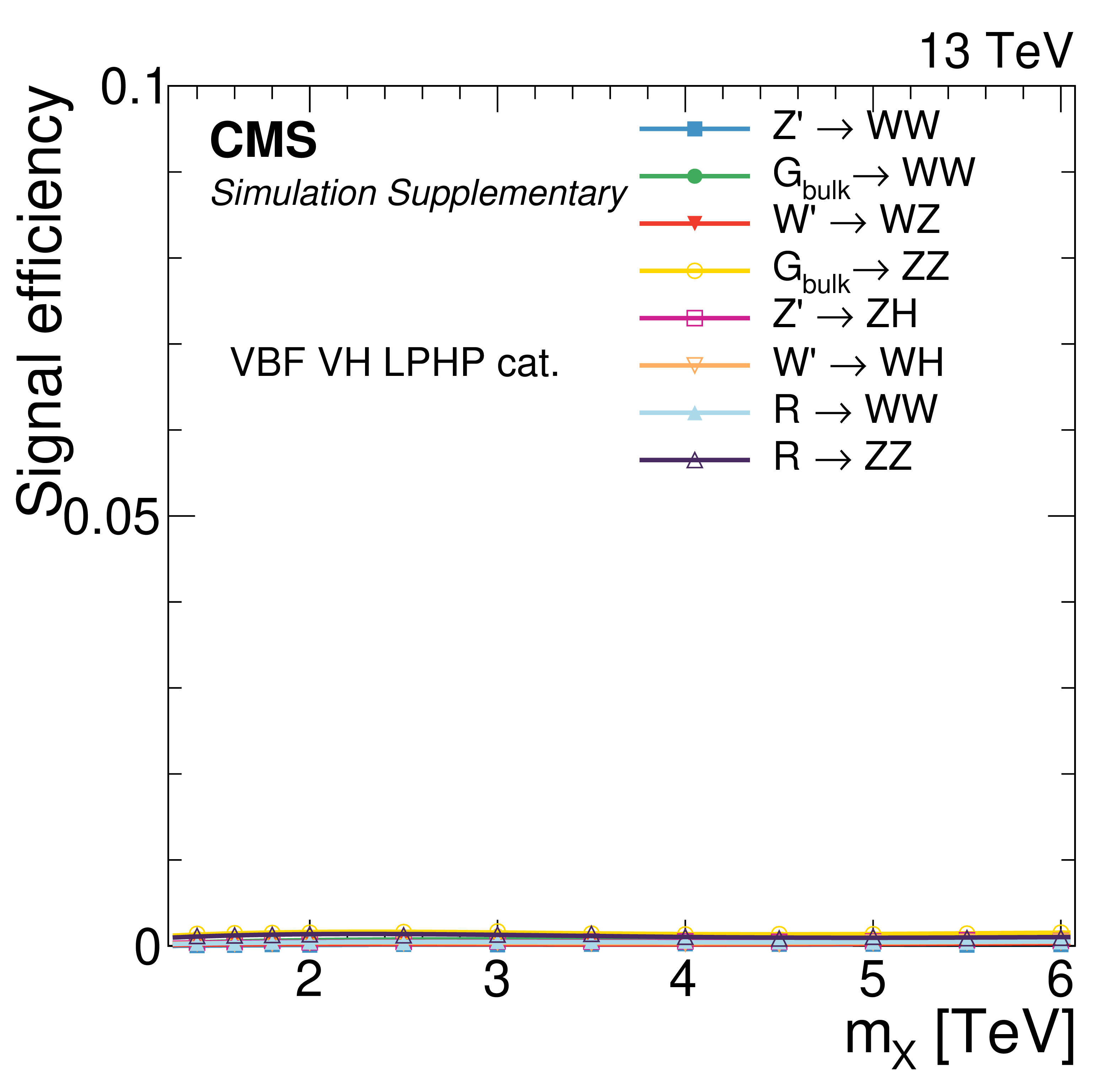
Additional Figure 4:
Signal efficiency in each of the categories as a function of the resonance mass $M_{\mathrm{X}}$ for all VBF signal models under consideration. The estimates from MC simulation (markers) are interpolated with a functional form (lines). |

png pdf |
Additional Figure 4-a:
Signal efficiency in each of the categories as a function of the resonance mass $M_{\mathrm{X}}$ for all VBF signal models under consideration. The estimates from MC simulation (markers) are interpolated with a functional form (lines). |

png pdf |
Additional Figure 4-b:
Signal efficiency in each of the categories as a function of the resonance mass $M_{\mathrm{X}}$ for all VBF signal models under consideration. The estimates from MC simulation (markers) are interpolated with a functional form (lines). |

png pdf |
Additional Figure 4-c:
Signal efficiency in each of the categories as a function of the resonance mass $M_{\mathrm{X}}$ for all VBF signal models under consideration. The estimates from MC simulation (markers) are interpolated with a functional form (lines). |

png pdf |
Additional Figure 4-d:
Signal efficiency in each of the categories as a function of the resonance mass $M_{\mathrm{X}}$ for all VBF signal models under consideration. The estimates from MC simulation (markers) are interpolated with a functional form (lines). |

png pdf |
Additional Figure 4-e:
Signal efficiency in each of the categories as a function of the resonance mass $M_{\mathrm{X}}$ for all VBF signal models under consideration. The estimates from MC simulation (markers) are interpolated with a functional form (lines). |

png pdf |
Additional Figure 4-f:
Signal efficiency in each of the categories as a function of the resonance mass $M_{\mathrm{X}}$ for all VBF signal models under consideration. The estimates from MC simulation (markers) are interpolated with a functional form (lines). |

png pdf |
Additional Figure 4-g:
Signal efficiency in each of the categories as a function of the resonance mass $M_{\mathrm{X}}$ for all VBF signal models under consideration. The estimates from MC simulation (markers) are interpolated with a functional form (lines). |

png pdf |
Additional Figure 4-h:
Signal efficiency in each of the categories as a function of the resonance mass $M_{\mathrm{X}}$ for all VBF signal models under consideration. The estimates from MC simulation (markers) are interpolated with a functional form (lines). |

png pdf |
Additional Figure 4-i:
Signal efficiency in each of the categories as a function of the resonance mass $M_{\mathrm{X}}$ for all VBF signal models under consideration. The estimates from MC simulation (markers) are interpolated with a functional form (lines). |

png pdf |
Additional Figure 4-j:
Signal efficiency in each of the categories as a function of the resonance mass $M_{\mathrm{X}}$ for all VBF signal models under consideration. The estimates from MC simulation (markers) are interpolated with a functional form (lines). |

png pdf |
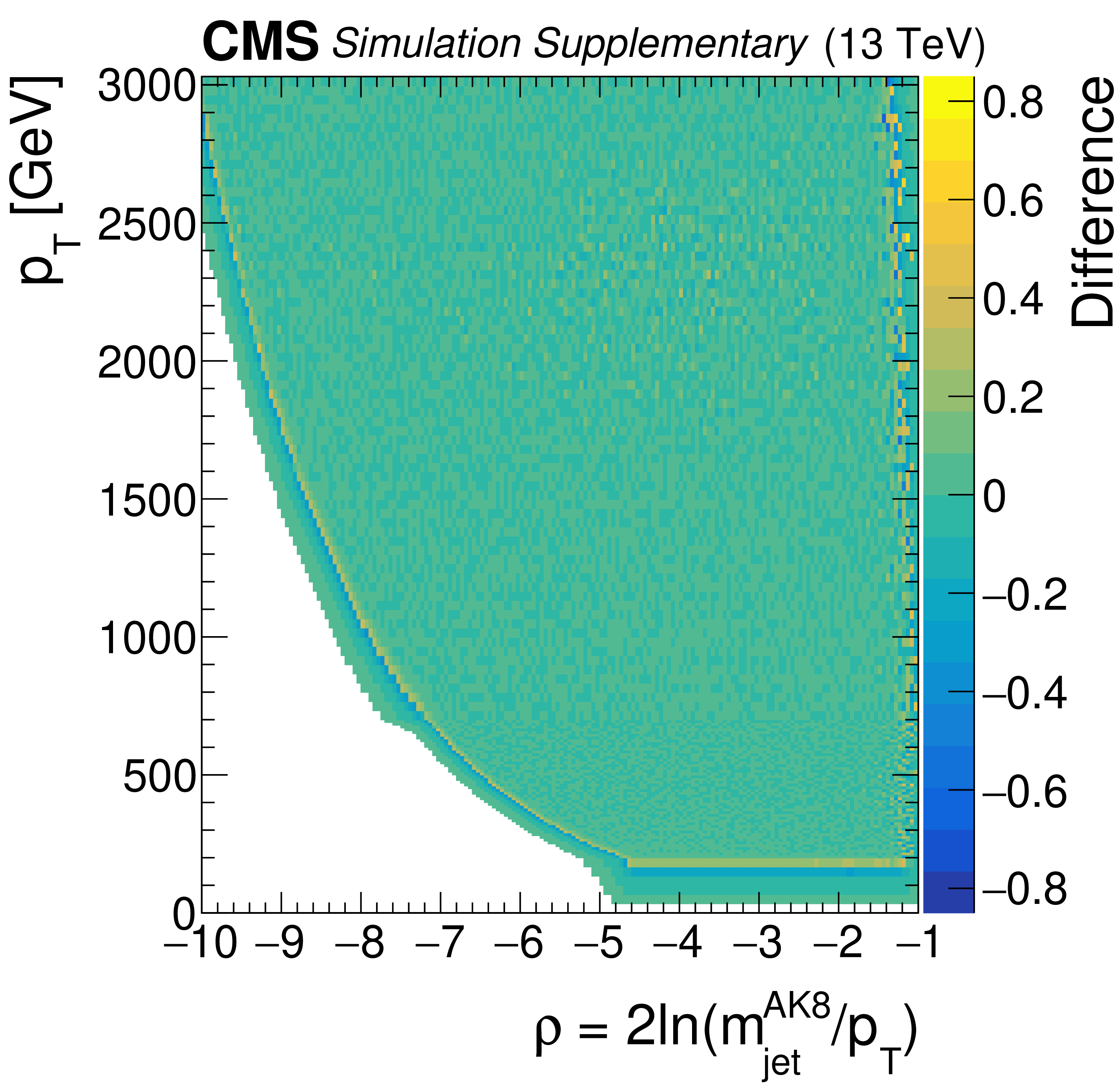
Additional Figure 5:
Left: Selection requirement on the $ \mathrm{q}\overline{\mathrm{q}} $ discriminator to obtain a 5% misidentification rate in QCD multijet simulation as a function of jet $ p_{\mathrm{T}} $ and $ \rho=2\ln(m_\text{jet}^{\mathrm{AK8}}/p_{\mathrm{T}}) $. Right: Difference in the requirement to be applied on the $ \mathrm{q}\overline{\mathrm{q}} $ tagger to obtain a 5% background misidentification rate between the nominal and a smoothed version of this histogram. |

png pdf |
Additional Figure 5-a:
Left: Selection requirement on the $ \mathrm{q}\overline{\mathrm{q}} $ discriminator to obtain a 5% misidentification rate in QCD multijet simulation as a function of jet $ p_{\mathrm{T}} $ and $ \rho=2\ln(m_\text{jet}^{\mathrm{AK8}}/p_{\mathrm{T}}) $. Right: Difference in the requirement to be applied on the $ \mathrm{q}\overline{\mathrm{q}} $ tagger to obtain a 5% background misidentification rate between the nominal and a smoothed version of this histogram. |
png pdf |
Additional Figure 5-b:
Left: Selection requirement on the $ \mathrm{q}\overline{\mathrm{q}} $ discriminator to obtain a 5% misidentification rate in QCD multijet simulation as a function of jet $ p_{\mathrm{T}} $ and $ \rho=2\ln(m_\text{jet}^{\mathrm{AK8}}/p_{\mathrm{T}}) $. Right: Difference in the requirement to be applied on the $ \mathrm{q}\overline{\mathrm{q}} $ tagger to obtain a 5% background misidentification rate between the nominal and a smoothed version of this histogram. |

png pdf |
Additional Figure 6:
Displays of an event with a reconstructed dijet invariant mass $ m_\mathrm{jj}^{\mathrm{AK8}}= $ 2.94 TeV in the DY/ggF VV HPHP category, with $ m_\text{jet1}^{\mathrm{AK8}}= $ 82 GeV and $ m_\text{jet2}^{\mathrm{AK8}}= $ 86 GeV, consistent with a WW, WZ or ZZ signal hypothesis. Reconstructed tracks are indicated as lines. Energy deposits in the electromagnetic and hadronic calorimeter are indicated as green and blue bars, respectively. The two leading AK8 jets have $ p_{\mathrm{T}}= $ 1.47 TeV, $ \eta= $ 0.27 and $ p_{\mathrm{T}}= $ 1.45 TeV, $ \eta= $ 0.17. |

png |
Additional Figure 6-a:
Displays of an event with a reconstructed dijet invariant mass $ m_\mathrm{jj}^{\mathrm{AK8}}= $ 2.94 TeV in the DY/ggF VV HPHP category, with $ m_\text{jet1}^{\mathrm{AK8}}= $ 82 GeV and $ m_\text{jet2}^{\mathrm{AK8}}= $ 86 GeV, consistent with a WW, WZ or ZZ signal hypothesis. Reconstructed tracks are indicated as lines. Energy deposits in the electromagnetic and hadronic calorimeter are indicated as green and blue bars, respectively. The two leading AK8 jets have $ p_{\mathrm{T}}= $ 1.47 TeV, $ \eta= $ 0.27 and $ p_{\mathrm{T}}= $ 1.45 TeV, $ \eta= $ 0.17. |

png |
Additional Figure 6-b:
Displays of an event with a reconstructed dijet invariant mass $ m_\mathrm{jj}^{\mathrm{AK8}}= $ 2.94 TeV in the DY/ggF VV HPHP category, with $ m_\text{jet1}^{\mathrm{AK8}}= $ 82 GeV and $ m_\text{jet2}^{\mathrm{AK8}}= $ 86 GeV, consistent with a WW, WZ or ZZ signal hypothesis. Reconstructed tracks are indicated as lines. Energy deposits in the electromagnetic and hadronic calorimeter are indicated as green and blue bars, respectively. The two leading AK8 jets have $ p_{\mathrm{T}}= $ 1.47 TeV, $ \eta= $ 0.27 and $ p_{\mathrm{T}}= $ 1.45 TeV, $ \eta= $ 0.17. |

png pdf |
Additional Figure 7:
Projections of PYTHIA8 MC simulation of the QCD multijet background distribution onto the $ m_\text{jet1}^{\mathrm{AK8}} $ (left), $ m_\text{jet2}^{\mathrm{AK8}} $ (middle), and $ m_\mathrm{jj}^{\mathrm{AK8}} $ (right) dimensions are compared to the nominal QCD background template and the five alternate shapes added to the fit as shape nuisance parameters for the VH HPHP (upper) and VV HPHP (lower) categories. |

png pdf |
Additional Figure 7-a:
Projections of PYTHIA8 MC simulation of the QCD multijet background distribution onto the $ m_\text{jet1}^{\mathrm{AK8}} $ (left), $ m_\text{jet2}^{\mathrm{AK8}} $ (middle), and $ m_\mathrm{jj}^{\mathrm{AK8}} $ (right) dimensions are compared to the nominal QCD background template and the five alternate shapes added to the fit as shape nuisance parameters for the VH HPHP (upper) and VV HPHP (lower) categories. |

png pdf |
Additional Figure 7-b:
Projections of PYTHIA8 MC simulation of the QCD multijet background distribution onto the $ m_\text{jet1}^{\mathrm{AK8}} $ (left), $ m_\text{jet2}^{\mathrm{AK8}} $ (middle), and $ m_\mathrm{jj}^{\mathrm{AK8}} $ (right) dimensions are compared to the nominal QCD background template and the five alternate shapes added to the fit as shape nuisance parameters for the VH HPHP (upper) and VV HPHP (lower) categories. |

png pdf |
Additional Figure 7-c:
Projections of PYTHIA8 MC simulation of the QCD multijet background distribution onto the $ m_\text{jet1}^{\mathrm{AK8}} $ (left), $ m_\text{jet2}^{\mathrm{AK8}} $ (middle), and $ m_\mathrm{jj}^{\mathrm{AK8}} $ (right) dimensions are compared to the nominal QCD background template and the five alternate shapes added to the fit as shape nuisance parameters for the VH HPHP (upper) and VV HPHP (lower) categories. |

png pdf |
Additional Figure 7-d:
Projections of PYTHIA8 MC simulation of the QCD multijet background distribution onto the $ m_\text{jet1}^{\mathrm{AK8}} $ (left), $ m_\text{jet2}^{\mathrm{AK8}} $ (middle), and $ m_\mathrm{jj}^{\mathrm{AK8}} $ (right) dimensions are compared to the nominal QCD background template and the five alternate shapes added to the fit as shape nuisance parameters for the VH HPHP (upper) and VV HPHP (lower) categories. |

png pdf |
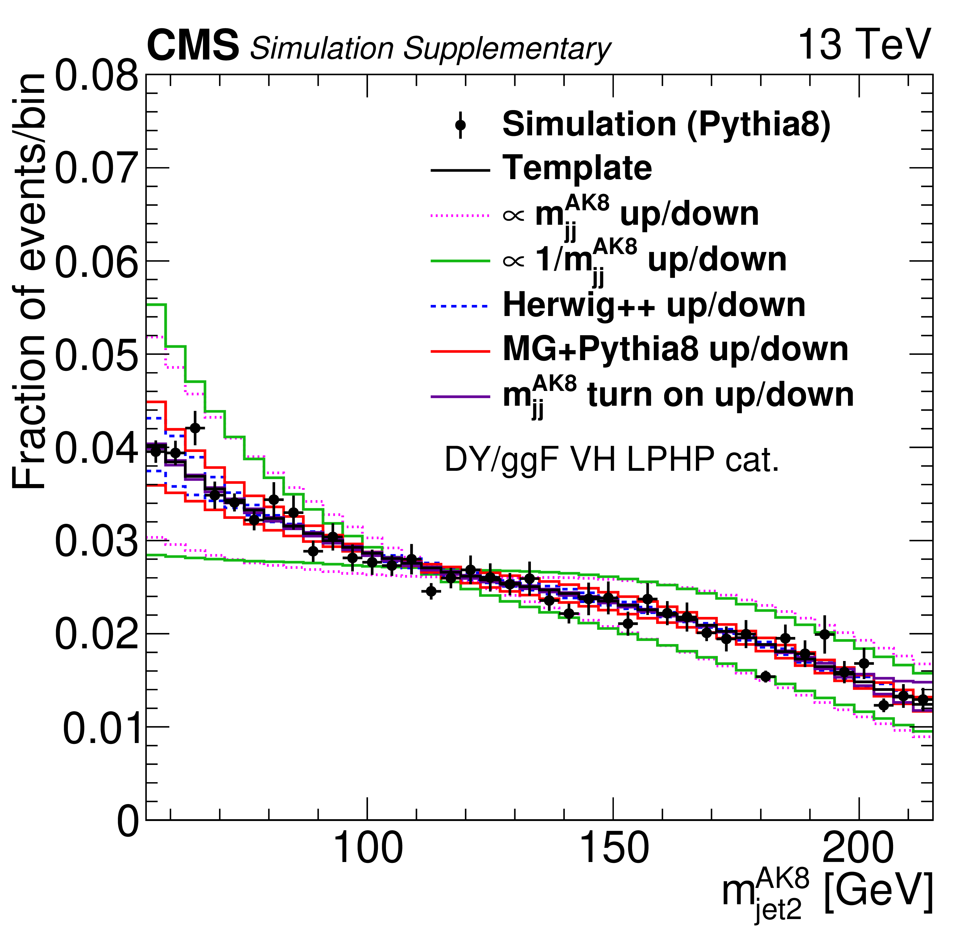
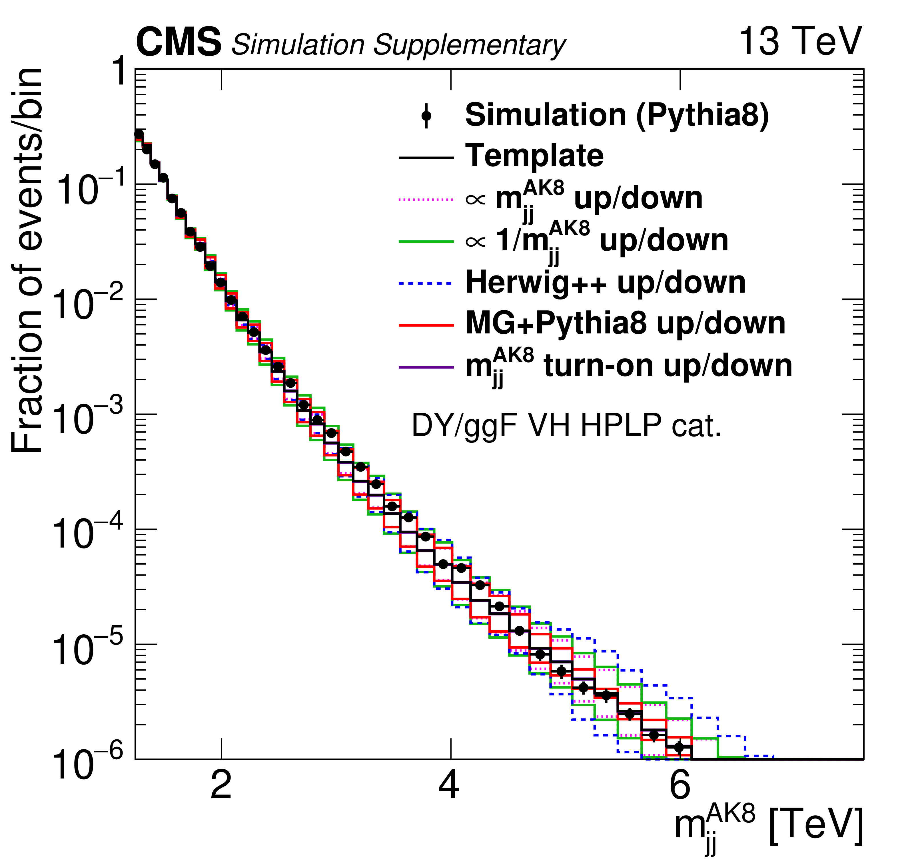
Additional Figure 8:
Projections of PYTHIA8 MC simulation of the QCD multijet background distribution onto the $ m_\text{jet1}^{\mathrm{AK8}} $ (left), $ m_\text{jet2}^{\mathrm{AK8}} $ (middle), and $ m_\mathrm{jj}^{\mathrm{AK8}} $ (right) dimensions are compared to the nominal QCD background template and the five alternate shapes added to the fit as shape nuisance parameters for the VH LPHP (upper), VH HPLP (middle), and VV HPLP (lower) categories. |

png pdf |
Additional Figure 8-a:
Projections of PYTHIA8 MC simulation of the QCD multijet background distribution onto the $ m_\text{jet1}^{\mathrm{AK8}} $ (left), $ m_\text{jet2}^{\mathrm{AK8}} $ (middle), and $ m_\mathrm{jj}^{\mathrm{AK8}} $ (right) dimensions are compared to the nominal QCD background template and the five alternate shapes added to the fit as shape nuisance parameters for the VH LPHP (upper), VH HPLP (middle), and VV HPLP (lower) categories. |
png pdf |
Additional Figure 8-b:
Projections of PYTHIA8 MC simulation of the QCD multijet background distribution onto the $ m_\text{jet1}^{\mathrm{AK8}} $ (left), $ m_\text{jet2}^{\mathrm{AK8}} $ (middle), and $ m_\mathrm{jj}^{\mathrm{AK8}} $ (right) dimensions are compared to the nominal QCD background template and the five alternate shapes added to the fit as shape nuisance parameters for the VH LPHP (upper), VH HPLP (middle), and VV HPLP (lower) categories. |

png pdf |
Additional Figure 8-c:
Projections of PYTHIA8 MC simulation of the QCD multijet background distribution onto the $ m_\text{jet1}^{\mathrm{AK8}} $ (left), $ m_\text{jet2}^{\mathrm{AK8}} $ (middle), and $ m_\mathrm{jj}^{\mathrm{AK8}} $ (right) dimensions are compared to the nominal QCD background template and the five alternate shapes added to the fit as shape nuisance parameters for the VH LPHP (upper), VH HPLP (middle), and VV HPLP (lower) categories. |

png pdf |
Additional Figure 8-d:
Projections of PYTHIA8 MC simulation of the QCD multijet background distribution onto the $ m_\text{jet1}^{\mathrm{AK8}} $ (left), $ m_\text{jet2}^{\mathrm{AK8}} $ (middle), and $ m_\mathrm{jj}^{\mathrm{AK8}} $ (right) dimensions are compared to the nominal QCD background template and the five alternate shapes added to the fit as shape nuisance parameters for the VH LPHP (upper), VH HPLP (middle), and VV HPLP (lower) categories. |

png pdf |
Additional Figure 8-e:
Projections of PYTHIA8 MC simulation of the QCD multijet background distribution onto the $ m_\text{jet1}^{\mathrm{AK8}} $ (left), $ m_\text{jet2}^{\mathrm{AK8}} $ (middle), and $ m_\mathrm{jj}^{\mathrm{AK8}} $ (right) dimensions are compared to the nominal QCD background template and the five alternate shapes added to the fit as shape nuisance parameters for the VH LPHP (upper), VH HPLP (middle), and VV HPLP (lower) categories. |
png pdf |
Additional Figure 8-f:
Projections of PYTHIA8 MC simulation of the QCD multijet background distribution onto the $ m_\text{jet1}^{\mathrm{AK8}} $ (left), $ m_\text{jet2}^{\mathrm{AK8}} $ (middle), and $ m_\mathrm{jj}^{\mathrm{AK8}} $ (right) dimensions are compared to the nominal QCD background template and the five alternate shapes added to the fit as shape nuisance parameters for the VH LPHP (upper), VH HPLP (middle), and VV HPLP (lower) categories. |

png pdf |
Additional Figure 8-g:
Projections of PYTHIA8 MC simulation of the QCD multijet background distribution onto the $ m_\text{jet1}^{\mathrm{AK8}} $ (left), $ m_\text{jet2}^{\mathrm{AK8}} $ (middle), and $ m_\mathrm{jj}^{\mathrm{AK8}} $ (right) dimensions are compared to the nominal QCD background template and the five alternate shapes added to the fit as shape nuisance parameters for the VH LPHP (upper), VH HPLP (middle), and VV HPLP (lower) categories. |

png pdf |
Additional Figure 8-h:
Projections of PYTHIA8 MC simulation of the QCD multijet background distribution onto the $ m_\text{jet1}^{\mathrm{AK8}} $ (left), $ m_\text{jet2}^{\mathrm{AK8}} $ (middle), and $ m_\mathrm{jj}^{\mathrm{AK8}} $ (right) dimensions are compared to the nominal QCD background template and the five alternate shapes added to the fit as shape nuisance parameters for the VH LPHP (upper), VH HPLP (middle), and VV HPLP (lower) categories. |

png pdf |
Additional Figure 8-i:
Projections of PYTHIA8 MC simulation of the QCD multijet background distribution onto the $ m_\text{jet1}^{\mathrm{AK8}} $ (left), $ m_\text{jet2}^{\mathrm{AK8}} $ (middle), and $ m_\mathrm{jj}^{\mathrm{AK8}} $ (right) dimensions are compared to the nominal QCD background template and the five alternate shapes added to the fit as shape nuisance parameters for the VH LPHP (upper), VH HPLP (middle), and VV HPLP (lower) categories. |
png pdf |
Additional Figure 9:
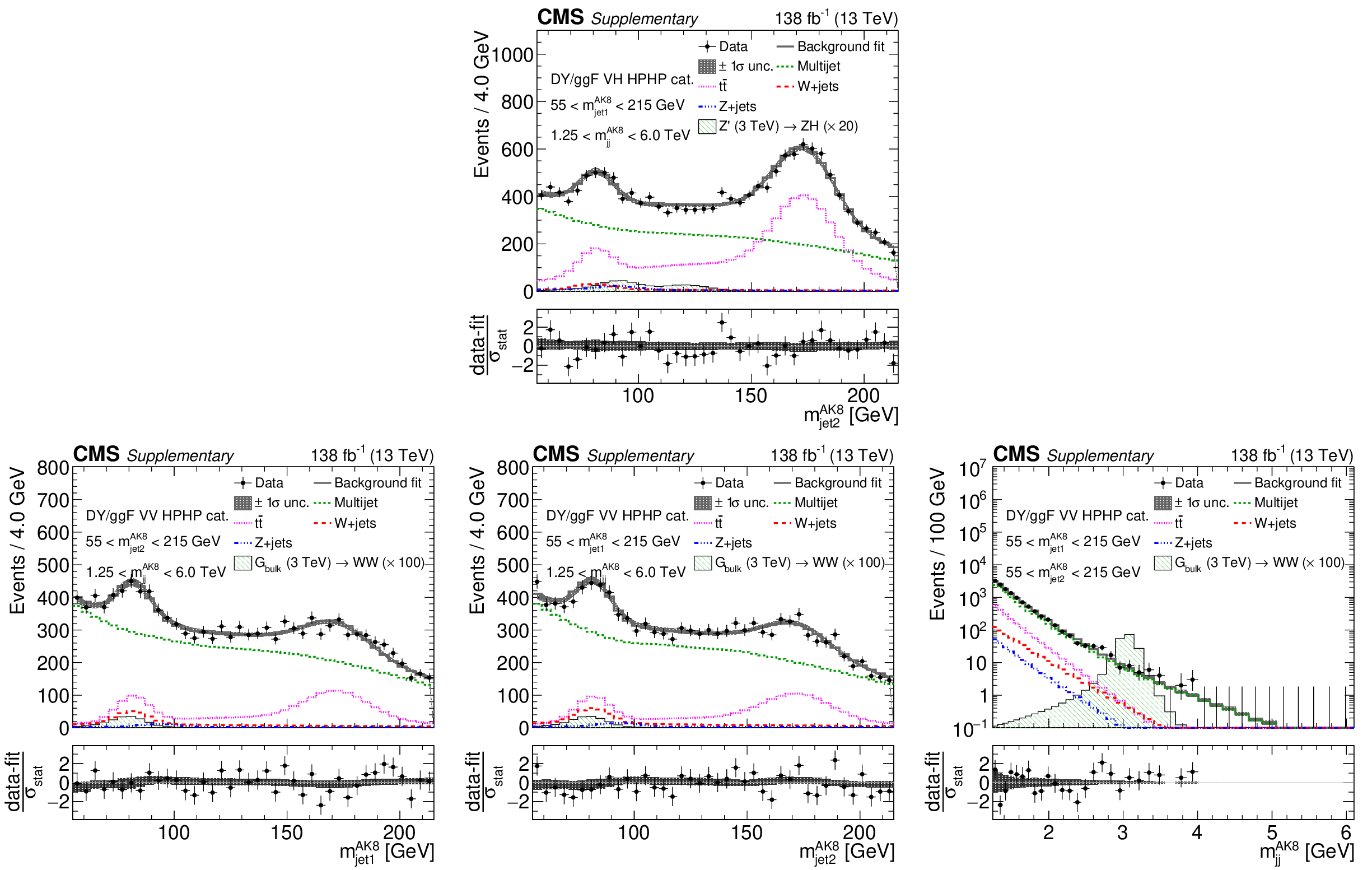
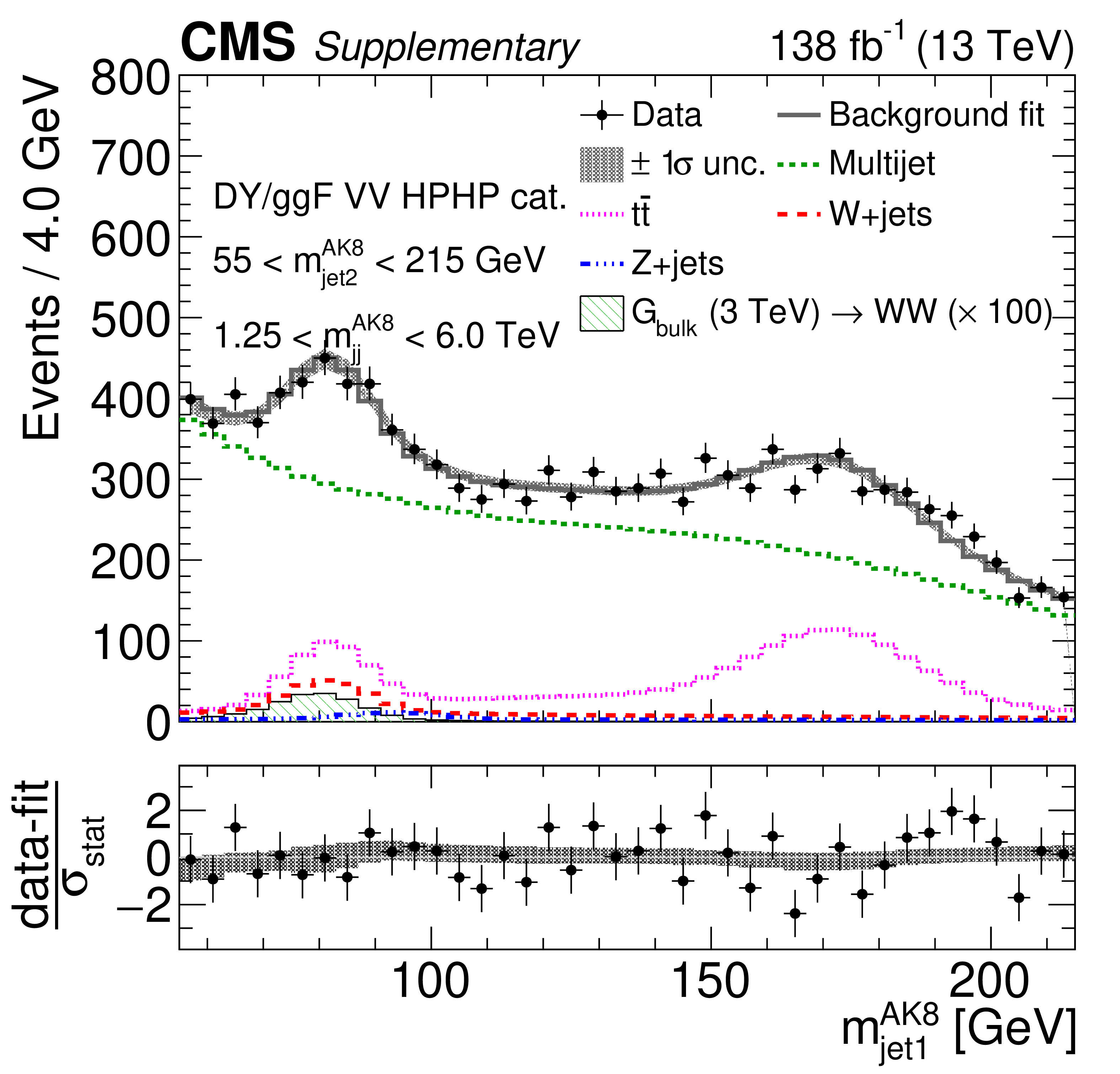
Comparison between the background post-fit and the data distributions of $ m_\text{jet1}^{\mathrm{AK8}} $ (left), $ m_\text{jet2}^{\mathrm{AK8}} $ (middle) and $ m_\mathrm{jj}^{\mathrm{AK8}} $ (right) in the DY/ggF VH HPHP (upper) and VV HPHP (lower) categories. The background shape uncertainty is shown as a gray shaded band around the result of the maximum likelihood fit to the data under the background-only assumption (gray solid line), and the statistical uncertainties in the data are shown as vertical bars. The various background components contributing to the total background fit are also shown with different line colors. An example of a signal distribution is overlaid, where the number of expected events is scaled by an arbitrary normalization factor. Shown below each mass plot is the difference between the data and the fit divided by the statistical uncertainty of the data; the uncertainty bar represents the statistical uncertainty only. The total uncertainty on the background estimate fitted to the data divided by the statistical uncertainty of the data is shown as a band. |

png pdf |
Additional Figure 9-a:
Comparison between the background post-fit and the data distributions of $ m_\text{jet1}^{\mathrm{AK8}} $ (left), $ m_\text{jet2}^{\mathrm{AK8}} $ (middle) and $ m_\mathrm{jj}^{\mathrm{AK8}} $ (right) in the DY/ggF VH HPHP (upper) and VV HPHP (lower) categories. The background shape uncertainty is shown as a gray shaded band around the result of the maximum likelihood fit to the data under the background-only assumption (gray solid line), and the statistical uncertainties in the data are shown as vertical bars. The various background components contributing to the total background fit are also shown with different line colors. An example of a signal distribution is overlaid, where the number of expected events is scaled by an arbitrary normalization factor. Shown below each mass plot is the difference between the data and the fit divided by the statistical uncertainty of the data; the uncertainty bar represents the statistical uncertainty only. The total uncertainty on the background estimate fitted to the data divided by the statistical uncertainty of the data is shown as a band. |
png pdf |
Additional Figure 9-b:
Comparison between the background post-fit and the data distributions of $ m_\text{jet1}^{\mathrm{AK8}} $ (left), $ m_\text{jet2}^{\mathrm{AK8}} $ (middle) and $ m_\mathrm{jj}^{\mathrm{AK8}} $ (right) in the DY/ggF VH HPHP (upper) and VV HPHP (lower) categories. The background shape uncertainty is shown as a gray shaded band around the result of the maximum likelihood fit to the data under the background-only assumption (gray solid line), and the statistical uncertainties in the data are shown as vertical bars. The various background components contributing to the total background fit are also shown with different line colors. An example of a signal distribution is overlaid, where the number of expected events is scaled by an arbitrary normalization factor. Shown below each mass plot is the difference between the data and the fit divided by the statistical uncertainty of the data; the uncertainty bar represents the statistical uncertainty only. The total uncertainty on the background estimate fitted to the data divided by the statistical uncertainty of the data is shown as a band. |

png pdf |
Additional Figure 9-c:
Comparison between the background post-fit and the data distributions of $ m_\text{jet1}^{\mathrm{AK8}} $ (left), $ m_\text{jet2}^{\mathrm{AK8}} $ (middle) and $ m_\mathrm{jj}^{\mathrm{AK8}} $ (right) in the DY/ggF VH HPHP (upper) and VV HPHP (lower) categories. The background shape uncertainty is shown as a gray shaded band around the result of the maximum likelihood fit to the data under the background-only assumption (gray solid line), and the statistical uncertainties in the data are shown as vertical bars. The various background components contributing to the total background fit are also shown with different line colors. An example of a signal distribution is overlaid, where the number of expected events is scaled by an arbitrary normalization factor. Shown below each mass plot is the difference between the data and the fit divided by the statistical uncertainty of the data; the uncertainty bar represents the statistical uncertainty only. The total uncertainty on the background estimate fitted to the data divided by the statistical uncertainty of the data is shown as a band. |

png pdf |
Additional Figure 9-d:
Comparison between the background post-fit and the data distributions of $ m_\text{jet1}^{\mathrm{AK8}} $ (left), $ m_\text{jet2}^{\mathrm{AK8}} $ (middle) and $ m_\mathrm{jj}^{\mathrm{AK8}} $ (right) in the DY/ggF VH HPHP (upper) and VV HPHP (lower) categories. The background shape uncertainty is shown as a gray shaded band around the result of the maximum likelihood fit to the data under the background-only assumption (gray solid line), and the statistical uncertainties in the data are shown as vertical bars. The various background components contributing to the total background fit are also shown with different line colors. An example of a signal distribution is overlaid, where the number of expected events is scaled by an arbitrary normalization factor. Shown below each mass plot is the difference between the data and the fit divided by the statistical uncertainty of the data; the uncertainty bar represents the statistical uncertainty only. The total uncertainty on the background estimate fitted to the data divided by the statistical uncertainty of the data is shown as a band. |

png pdf |
Additional Figure 10:
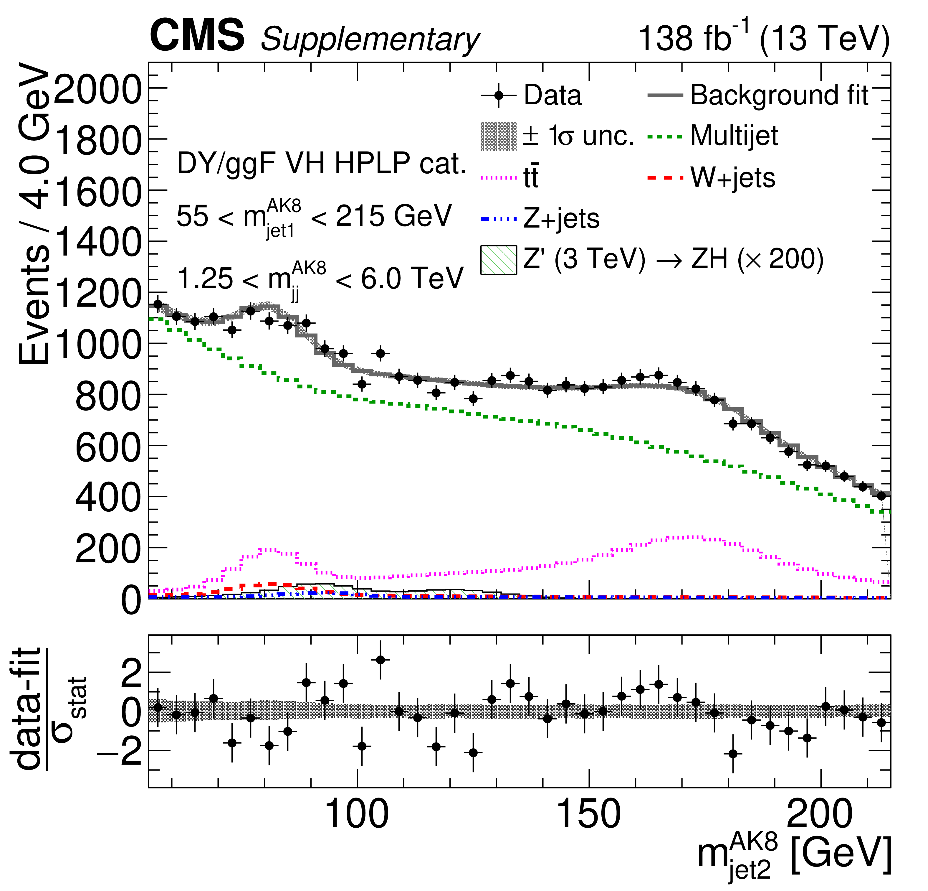
Comparison between the background post-fit and the data distributions of $ m_\text{jet1}^{\mathrm{AK8}} $ (left), $ m_\text{jet2}^{\mathrm{AK8}} $ (middle) and $ m_\mathrm{jj}^{\mathrm{AK8}} $ (right) in the DY/ggF VH LPHP (upper), DY/ggF VH HPLP (middle), and DY/ggF VV HPLP (lower) categories. The background shape uncertainty is shown as a gray shaded band around the result of the maximum likelihood fit to the data under the background-only assumption (gray solid line), and the statistical uncertainties in the data are shown as vertical bars. The various background components contributing to the total background fit are also shown with different line colors. An example of a signal distribution is overlaid, where the number of expected events is scaled by an arbitrary normalization factor. Shown below each mass plot is the difference between the data and the fit divided by the statistical uncertainty in the data; the uncertainty bar represents the statistical uncertainty only. The total uncertainty in the background estimate fitted to the data divided by the statistical uncertainty in the data is shown as a band. |

png pdf |
Additional Figure 10-a:
Comparison between the background post-fit and the data distributions of $ m_\text{jet1}^{\mathrm{AK8}} $ (left), $ m_\text{jet2}^{\mathrm{AK8}} $ (middle) and $ m_\mathrm{jj}^{\mathrm{AK8}} $ (right) in the DY/ggF VH LPHP (upper), DY/ggF VH HPLP (middle), and DY/ggF VV HPLP (lower) categories. The background shape uncertainty is shown as a gray shaded band around the result of the maximum likelihood fit to the data under the background-only assumption (gray solid line), and the statistical uncertainties in the data are shown as vertical bars. The various background components contributing to the total background fit are also shown with different line colors. An example of a signal distribution is overlaid, where the number of expected events is scaled by an arbitrary normalization factor. Shown below each mass plot is the difference between the data and the fit divided by the statistical uncertainty in the data; the uncertainty bar represents the statistical uncertainty only. The total uncertainty in the background estimate fitted to the data divided by the statistical uncertainty in the data is shown as a band. |

png pdf |
Additional Figure 10-b:
Comparison between the background post-fit and the data distributions of $ m_\text{jet1}^{\mathrm{AK8}} $ (left), $ m_\text{jet2}^{\mathrm{AK8}} $ (middle) and $ m_\mathrm{jj}^{\mathrm{AK8}} $ (right) in the DY/ggF VH LPHP (upper), DY/ggF VH HPLP (middle), and DY/ggF VV HPLP (lower) categories. The background shape uncertainty is shown as a gray shaded band around the result of the maximum likelihood fit to the data under the background-only assumption (gray solid line), and the statistical uncertainties in the data are shown as vertical bars. The various background components contributing to the total background fit are also shown with different line colors. An example of a signal distribution is overlaid, where the number of expected events is scaled by an arbitrary normalization factor. Shown below each mass plot is the difference between the data and the fit divided by the statistical uncertainty in the data; the uncertainty bar represents the statistical uncertainty only. The total uncertainty in the background estimate fitted to the data divided by the statistical uncertainty in the data is shown as a band. |

png pdf |
Additional Figure 10-c:
Comparison between the background post-fit and the data distributions of $ m_\text{jet1}^{\mathrm{AK8}} $ (left), $ m_\text{jet2}^{\mathrm{AK8}} $ (middle) and $ m_\mathrm{jj}^{\mathrm{AK8}} $ (right) in the DY/ggF VH LPHP (upper), DY/ggF VH HPLP (middle), and DY/ggF VV HPLP (lower) categories. The background shape uncertainty is shown as a gray shaded band around the result of the maximum likelihood fit to the data under the background-only assumption (gray solid line), and the statistical uncertainties in the data are shown as vertical bars. The various background components contributing to the total background fit are also shown with different line colors. An example of a signal distribution is overlaid, where the number of expected events is scaled by an arbitrary normalization factor. Shown below each mass plot is the difference between the data and the fit divided by the statistical uncertainty in the data; the uncertainty bar represents the statistical uncertainty only. The total uncertainty in the background estimate fitted to the data divided by the statistical uncertainty in the data is shown as a band. |

png pdf |
Additional Figure 10-d:
Comparison between the background post-fit and the data distributions of $ m_\text{jet1}^{\mathrm{AK8}} $ (left), $ m_\text{jet2}^{\mathrm{AK8}} $ (middle) and $ m_\mathrm{jj}^{\mathrm{AK8}} $ (right) in the DY/ggF VH LPHP (upper), DY/ggF VH HPLP (middle), and DY/ggF VV HPLP (lower) categories. The background shape uncertainty is shown as a gray shaded band around the result of the maximum likelihood fit to the data under the background-only assumption (gray solid line), and the statistical uncertainties in the data are shown as vertical bars. The various background components contributing to the total background fit are also shown with different line colors. An example of a signal distribution is overlaid, where the number of expected events is scaled by an arbitrary normalization factor. Shown below each mass plot is the difference between the data and the fit divided by the statistical uncertainty in the data; the uncertainty bar represents the statistical uncertainty only. The total uncertainty in the background estimate fitted to the data divided by the statistical uncertainty in the data is shown as a band. |
png pdf |
Additional Figure 10-e:
Comparison between the background post-fit and the data distributions of $ m_\text{jet1}^{\mathrm{AK8}} $ (left), $ m_\text{jet2}^{\mathrm{AK8}} $ (middle) and $ m_\mathrm{jj}^{\mathrm{AK8}} $ (right) in the DY/ggF VH LPHP (upper), DY/ggF VH HPLP (middle), and DY/ggF VV HPLP (lower) categories. The background shape uncertainty is shown as a gray shaded band around the result of the maximum likelihood fit to the data under the background-only assumption (gray solid line), and the statistical uncertainties in the data are shown as vertical bars. The various background components contributing to the total background fit are also shown with different line colors. An example of a signal distribution is overlaid, where the number of expected events is scaled by an arbitrary normalization factor. Shown below each mass plot is the difference between the data and the fit divided by the statistical uncertainty in the data; the uncertainty bar represents the statistical uncertainty only. The total uncertainty in the background estimate fitted to the data divided by the statistical uncertainty in the data is shown as a band. |

png pdf |
Additional Figure 10-f:
Comparison between the background post-fit and the data distributions of $ m_\text{jet1}^{\mathrm{AK8}} $ (left), $ m_\text{jet2}^{\mathrm{AK8}} $ (middle) and $ m_\mathrm{jj}^{\mathrm{AK8}} $ (right) in the DY/ggF VH LPHP (upper), DY/ggF VH HPLP (middle), and DY/ggF VV HPLP (lower) categories. The background shape uncertainty is shown as a gray shaded band around the result of the maximum likelihood fit to the data under the background-only assumption (gray solid line), and the statistical uncertainties in the data are shown as vertical bars. The various background components contributing to the total background fit are also shown with different line colors. An example of a signal distribution is overlaid, where the number of expected events is scaled by an arbitrary normalization factor. Shown below each mass plot is the difference between the data and the fit divided by the statistical uncertainty in the data; the uncertainty bar represents the statistical uncertainty only. The total uncertainty in the background estimate fitted to the data divided by the statistical uncertainty in the data is shown as a band. |

png pdf |
Additional Figure 10-g:
Comparison between the background post-fit and the data distributions of $ m_\text{jet1}^{\mathrm{AK8}} $ (left), $ m_\text{jet2}^{\mathrm{AK8}} $ (middle) and $ m_\mathrm{jj}^{\mathrm{AK8}} $ (right) in the DY/ggF VH LPHP (upper), DY/ggF VH HPLP (middle), and DY/ggF VV HPLP (lower) categories. The background shape uncertainty is shown as a gray shaded band around the result of the maximum likelihood fit to the data under the background-only assumption (gray solid line), and the statistical uncertainties in the data are shown as vertical bars. The various background components contributing to the total background fit are also shown with different line colors. An example of a signal distribution is overlaid, where the number of expected events is scaled by an arbitrary normalization factor. Shown below each mass plot is the difference between the data and the fit divided by the statistical uncertainty in the data; the uncertainty bar represents the statistical uncertainty only. The total uncertainty in the background estimate fitted to the data divided by the statistical uncertainty in the data is shown as a band. |

png pdf |
Additional Figure 10-h:
Comparison between the background post-fit and the data distributions of $ m_\text{jet1}^{\mathrm{AK8}} $ (left), $ m_\text{jet2}^{\mathrm{AK8}} $ (middle) and $ m_\mathrm{jj}^{\mathrm{AK8}} $ (right) in the DY/ggF VH LPHP (upper), DY/ggF VH HPLP (middle), and DY/ggF VV HPLP (lower) categories. The background shape uncertainty is shown as a gray shaded band around the result of the maximum likelihood fit to the data under the background-only assumption (gray solid line), and the statistical uncertainties in the data are shown as vertical bars. The various background components contributing to the total background fit are also shown with different line colors. An example of a signal distribution is overlaid, where the number of expected events is scaled by an arbitrary normalization factor. Shown below each mass plot is the difference between the data and the fit divided by the statistical uncertainty in the data; the uncertainty bar represents the statistical uncertainty only. The total uncertainty in the background estimate fitted to the data divided by the statistical uncertainty in the data is shown as a band. |

png pdf |
Additional Figure 10-i:
Comparison between the background post-fit and the data distributions of $ m_\text{jet1}^{\mathrm{AK8}} $ (left), $ m_\text{jet2}^{\mathrm{AK8}} $ (middle) and $ m_\mathrm{jj}^{\mathrm{AK8}} $ (right) in the DY/ggF VH LPHP (upper), DY/ggF VH HPLP (middle), and DY/ggF VV HPLP (lower) categories. The background shape uncertainty is shown as a gray shaded band around the result of the maximum likelihood fit to the data under the background-only assumption (gray solid line), and the statistical uncertainties in the data are shown as vertical bars. The various background components contributing to the total background fit are also shown with different line colors. An example of a signal distribution is overlaid, where the number of expected events is scaled by an arbitrary normalization factor. Shown below each mass plot is the difference between the data and the fit divided by the statistical uncertainty in the data; the uncertainty bar represents the statistical uncertainty only. The total uncertainty in the background estimate fitted to the data divided by the statistical uncertainty in the data is shown as a band. |

png pdf |
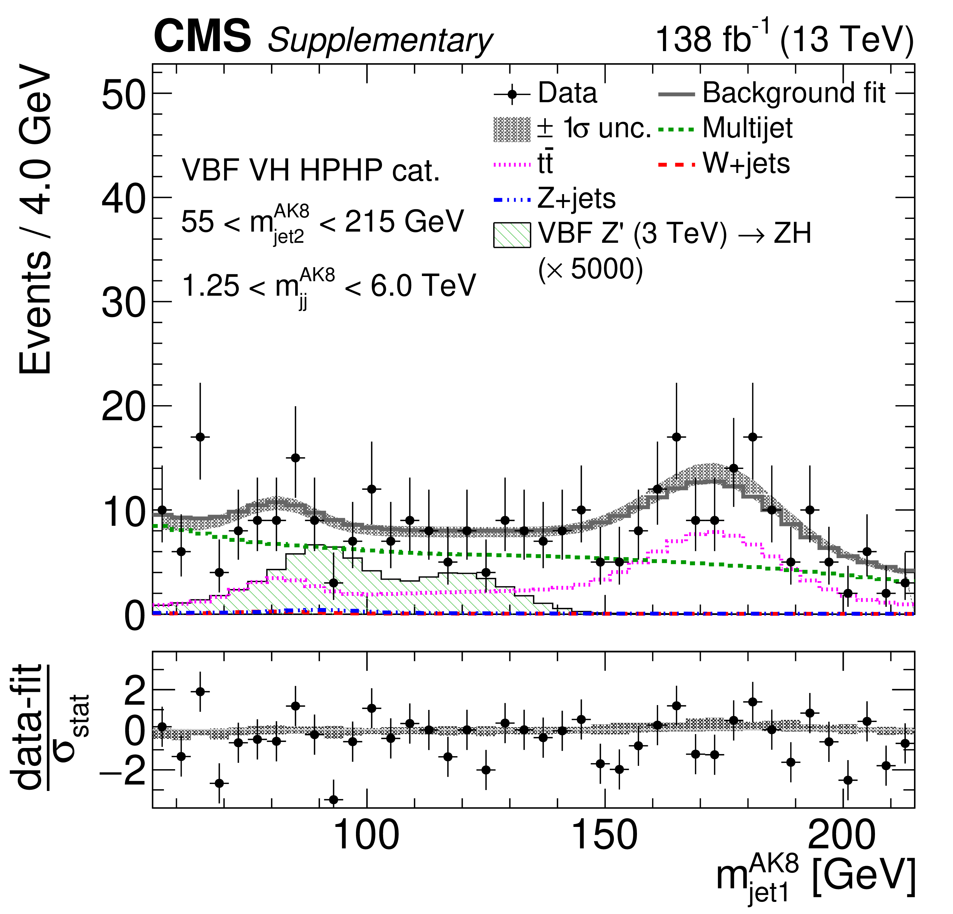
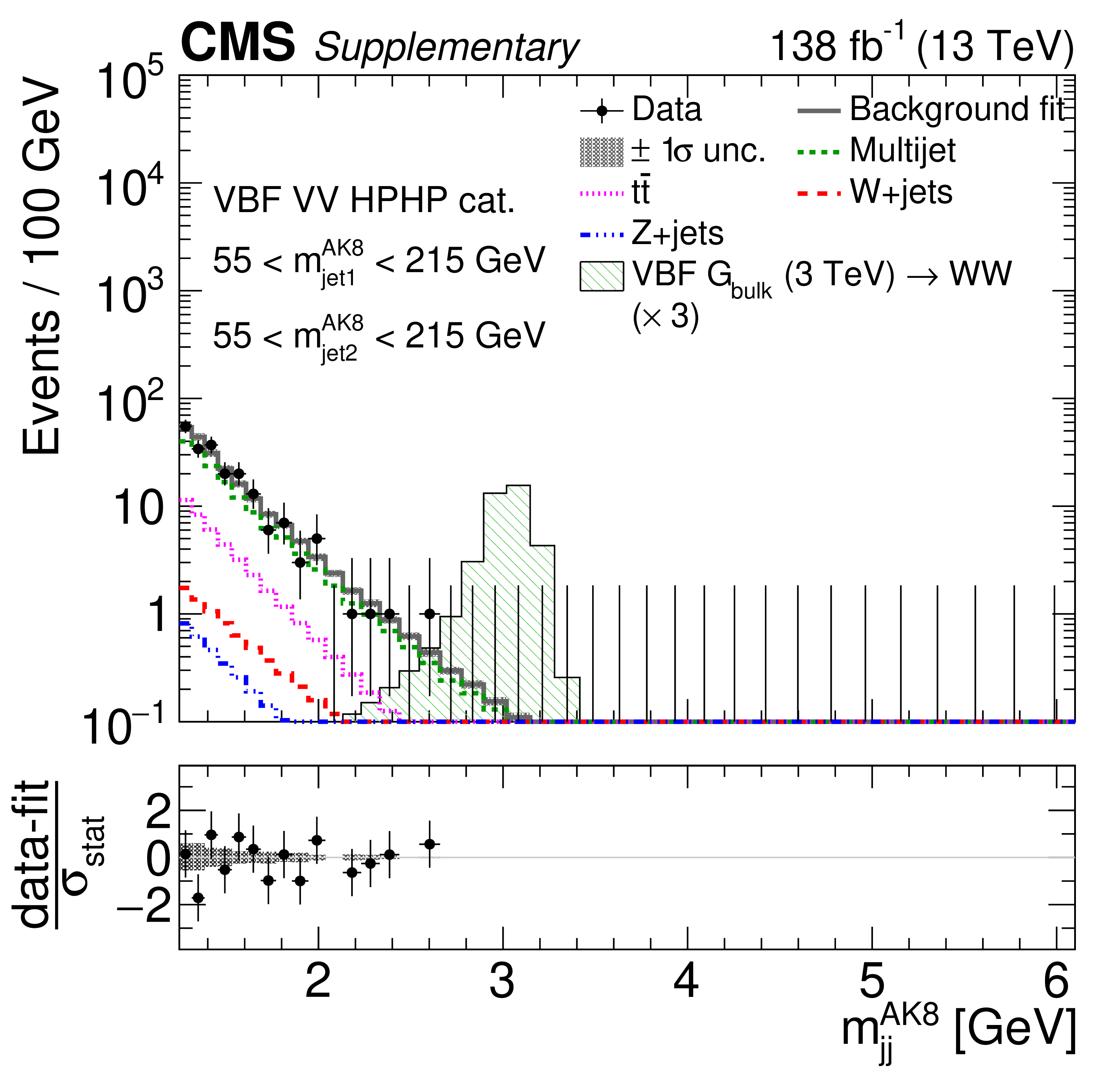
Additional Figure 11:
Comparison between the background post-fit and the data distributions of $ m_\text{jet1}^{\mathrm{AK8}} $ (left), $ m_\text{jet2}^{\mathrm{AK8}} $ (middle) and $ m_\mathrm{jj}^{\mathrm{AK8}} $ (right) in the VBF VH HPHP (upper) and VBF VV HPHP (lower) categories. The background shape uncertainty is shown as a gray shaded band around the result of the maximum likelihood fit to the data under the background-only assumption (gray solid line), and the statistical uncertainties in the data are shown as vertical bars. The various background components contributing to the total background fit are also shown with different line colors. An example of a signal distribution is overlaid, where the number of expected events is scaled by an arbitrary normalization factor. Shown below each mass plot is the difference between the data and the fit divided by the statistical uncertainty in the data; the uncertainty bar represents the statistical uncertainty only. The total uncertainty in the background estimate fitted to the data divided by the statistical uncertainty in the data is shown as a band. |
png pdf |
Additional Figure 11-a:
Comparison between the background post-fit and the data distributions of $ m_\text{jet1}^{\mathrm{AK8}} $ (left), $ m_\text{jet2}^{\mathrm{AK8}} $ (middle) and $ m_\mathrm{jj}^{\mathrm{AK8}} $ (right) in the VBF VH HPHP (upper) and VBF VV HPHP (lower) categories. The background shape uncertainty is shown as a gray shaded band around the result of the maximum likelihood fit to the data under the background-only assumption (gray solid line), and the statistical uncertainties in the data are shown as vertical bars. The various background components contributing to the total background fit are also shown with different line colors. An example of a signal distribution is overlaid, where the number of expected events is scaled by an arbitrary normalization factor. Shown below each mass plot is the difference between the data and the fit divided by the statistical uncertainty in the data; the uncertainty bar represents the statistical uncertainty only. The total uncertainty in the background estimate fitted to the data divided by the statistical uncertainty in the data is shown as a band. |

png pdf |
Additional Figure 11-b:
Comparison between the background post-fit and the data distributions of $ m_\text{jet1}^{\mathrm{AK8}} $ (left), $ m_\text{jet2}^{\mathrm{AK8}} $ (middle) and $ m_\mathrm{jj}^{\mathrm{AK8}} $ (right) in the VBF VH HPHP (upper) and VBF VV HPHP (lower) categories. The background shape uncertainty is shown as a gray shaded band around the result of the maximum likelihood fit to the data under the background-only assumption (gray solid line), and the statistical uncertainties in the data are shown as vertical bars. The various background components contributing to the total background fit are also shown with different line colors. An example of a signal distribution is overlaid, where the number of expected events is scaled by an arbitrary normalization factor. Shown below each mass plot is the difference between the data and the fit divided by the statistical uncertainty in the data; the uncertainty bar represents the statistical uncertainty only. The total uncertainty in the background estimate fitted to the data divided by the statistical uncertainty in the data is shown as a band. |

png pdf |
Additional Figure 11-c:
Comparison between the background post-fit and the data distributions of $ m_\text{jet1}^{\mathrm{AK8}} $ (left), $ m_\text{jet2}^{\mathrm{AK8}} $ (middle) and $ m_\mathrm{jj}^{\mathrm{AK8}} $ (right) in the VBF VH HPHP (upper) and VBF VV HPHP (lower) categories. The background shape uncertainty is shown as a gray shaded band around the result of the maximum likelihood fit to the data under the background-only assumption (gray solid line), and the statistical uncertainties in the data are shown as vertical bars. The various background components contributing to the total background fit are also shown with different line colors. An example of a signal distribution is overlaid, where the number of expected events is scaled by an arbitrary normalization factor. Shown below each mass plot is the difference between the data and the fit divided by the statistical uncertainty in the data; the uncertainty bar represents the statistical uncertainty only. The total uncertainty in the background estimate fitted to the data divided by the statistical uncertainty in the data is shown as a band. |

png pdf |
Additional Figure 11-d:
Comparison between the background post-fit and the data distributions of $ m_\text{jet1}^{\mathrm{AK8}} $ (left), $ m_\text{jet2}^{\mathrm{AK8}} $ (middle) and $ m_\mathrm{jj}^{\mathrm{AK8}} $ (right) in the VBF VH HPHP (upper) and VBF VV HPHP (lower) categories. The background shape uncertainty is shown as a gray shaded band around the result of the maximum likelihood fit to the data under the background-only assumption (gray solid line), and the statistical uncertainties in the data are shown as vertical bars. The various background components contributing to the total background fit are also shown with different line colors. An example of a signal distribution is overlaid, where the number of expected events is scaled by an arbitrary normalization factor. Shown below each mass plot is the difference between the data and the fit divided by the statistical uncertainty in the data; the uncertainty bar represents the statistical uncertainty only. The total uncertainty in the background estimate fitted to the data divided by the statistical uncertainty in the data is shown as a band. |

png pdf |
Additional Figure 11-e:
Comparison between the background post-fit and the data distributions of $ m_\text{jet1}^{\mathrm{AK8}} $ (left), $ m_\text{jet2}^{\mathrm{AK8}} $ (middle) and $ m_\mathrm{jj}^{\mathrm{AK8}} $ (right) in the VBF VH HPHP (upper) and VBF VV HPHP (lower) categories. The background shape uncertainty is shown as a gray shaded band around the result of the maximum likelihood fit to the data under the background-only assumption (gray solid line), and the statistical uncertainties in the data are shown as vertical bars. The various background components contributing to the total background fit are also shown with different line colors. An example of a signal distribution is overlaid, where the number of expected events is scaled by an arbitrary normalization factor. Shown below each mass plot is the difference between the data and the fit divided by the statistical uncertainty in the data; the uncertainty bar represents the statistical uncertainty only. The total uncertainty in the background estimate fitted to the data divided by the statistical uncertainty in the data is shown as a band. |
png pdf |
Additional Figure 11-f:
Comparison between the background post-fit and the data distributions of $ m_\text{jet1}^{\mathrm{AK8}} $ (left), $ m_\text{jet2}^{\mathrm{AK8}} $ (middle) and $ m_\mathrm{jj}^{\mathrm{AK8}} $ (right) in the VBF VH HPHP (upper) and VBF VV HPHP (lower) categories. The background shape uncertainty is shown as a gray shaded band around the result of the maximum likelihood fit to the data under the background-only assumption (gray solid line), and the statistical uncertainties in the data are shown as vertical bars. The various background components contributing to the total background fit are also shown with different line colors. An example of a signal distribution is overlaid, where the number of expected events is scaled by an arbitrary normalization factor. Shown below each mass plot is the difference between the data and the fit divided by the statistical uncertainty in the data; the uncertainty bar represents the statistical uncertainty only. The total uncertainty in the background estimate fitted to the data divided by the statistical uncertainty in the data is shown as a band. |

png pdf |
Additional Figure 12:
Comparison between the background post-fit and the data distributions of $ m_\text{jet1}^{\mathrm{AK8}} $ (left), $ m_\text{jet2}^{\mathrm{AK8}} $ (middle) and $ m_\mathrm{jj}^{\mathrm{AK8}} $ (right) in the VBF VH LPHP (upper), VBF VH HPLP (middle), and VBF VV HPLP (lower) categories. The background shape uncertainty is shown as a gray shaded band around the result of the maximum likelihood fit to the data under the background-only assumption (gray solid line), and the statistical uncertainties in the data are shown as vertical bars. The various background components contributing to the total background fit are also shown with different line colors. An example of a signal distribution is overlaid, where the number of expected events is scaled by an arbitrary normalization factor. Shown below each mass plot is the difference between the data and the fit divided by the statistical uncertainty in the data; the uncertainty bar represents the statistical uncertainty only. The total uncertainty in the background estimate fitted to the data divided by the statistical uncertainty in the data is shown as a band. |

png pdf |
Additional Figure 12-a:
Comparison between the background post-fit and the data distributions of $ m_\text{jet1}^{\mathrm{AK8}} $ (left), $ m_\text{jet2}^{\mathrm{AK8}} $ (middle) and $ m_\mathrm{jj}^{\mathrm{AK8}} $ (right) in the VBF VH LPHP (upper), VBF VH HPLP (middle), and VBF VV HPLP (lower) categories. The background shape uncertainty is shown as a gray shaded band around the result of the maximum likelihood fit to the data under the background-only assumption (gray solid line), and the statistical uncertainties in the data are shown as vertical bars. The various background components contributing to the total background fit are also shown with different line colors. An example of a signal distribution is overlaid, where the number of expected events is scaled by an arbitrary normalization factor. Shown below each mass plot is the difference between the data and the fit divided by the statistical uncertainty in the data; the uncertainty bar represents the statistical uncertainty only. The total uncertainty in the background estimate fitted to the data divided by the statistical uncertainty in the data is shown as a band. |

png pdf |
Additional Figure 12-b:
Comparison between the background post-fit and the data distributions of $ m_\text{jet1}^{\mathrm{AK8}} $ (left), $ m_\text{jet2}^{\mathrm{AK8}} $ (middle) and $ m_\mathrm{jj}^{\mathrm{AK8}} $ (right) in the VBF VH LPHP (upper), VBF VH HPLP (middle), and VBF VV HPLP (lower) categories. The background shape uncertainty is shown as a gray shaded band around the result of the maximum likelihood fit to the data under the background-only assumption (gray solid line), and the statistical uncertainties in the data are shown as vertical bars. The various background components contributing to the total background fit are also shown with different line colors. An example of a signal distribution is overlaid, where the number of expected events is scaled by an arbitrary normalization factor. Shown below each mass plot is the difference between the data and the fit divided by the statistical uncertainty in the data; the uncertainty bar represents the statistical uncertainty only. The total uncertainty in the background estimate fitted to the data divided by the statistical uncertainty in the data is shown as a band. |

png pdf |
Additional Figure 12-c:
Comparison between the background post-fit and the data distributions of $ m_\text{jet1}^{\mathrm{AK8}} $ (left), $ m_\text{jet2}^{\mathrm{AK8}} $ (middle) and $ m_\mathrm{jj}^{\mathrm{AK8}} $ (right) in the VBF VH LPHP (upper), VBF VH HPLP (middle), and VBF VV HPLP (lower) categories. The background shape uncertainty is shown as a gray shaded band around the result of the maximum likelihood fit to the data under the background-only assumption (gray solid line), and the statistical uncertainties in the data are shown as vertical bars. The various background components contributing to the total background fit are also shown with different line colors. An example of a signal distribution is overlaid, where the number of expected events is scaled by an arbitrary normalization factor. Shown below each mass plot is the difference between the data and the fit divided by the statistical uncertainty in the data; the uncertainty bar represents the statistical uncertainty only. The total uncertainty in the background estimate fitted to the data divided by the statistical uncertainty in the data is shown as a band. |

png pdf |
Additional Figure 12-d:
Comparison between the background post-fit and the data distributions of $ m_\text{jet1}^{\mathrm{AK8}} $ (left), $ m_\text{jet2}^{\mathrm{AK8}} $ (middle) and $ m_\mathrm{jj}^{\mathrm{AK8}} $ (right) in the VBF VH LPHP (upper), VBF VH HPLP (middle), and VBF VV HPLP (lower) categories. The background shape uncertainty is shown as a gray shaded band around the result of the maximum likelihood fit to the data under the background-only assumption (gray solid line), and the statistical uncertainties in the data are shown as vertical bars. The various background components contributing to the total background fit are also shown with different line colors. An example of a signal distribution is overlaid, where the number of expected events is scaled by an arbitrary normalization factor. Shown below each mass plot is the difference between the data and the fit divided by the statistical uncertainty in the data; the uncertainty bar represents the statistical uncertainty only. The total uncertainty in the background estimate fitted to the data divided by the statistical uncertainty in the data is shown as a band. |

png pdf |
Additional Figure 12-e:
Comparison between the background post-fit and the data distributions of $ m_\text{jet1}^{\mathrm{AK8}} $ (left), $ m_\text{jet2}^{\mathrm{AK8}} $ (middle) and $ m_\mathrm{jj}^{\mathrm{AK8}} $ (right) in the VBF VH LPHP (upper), VBF VH HPLP (middle), and VBF VV HPLP (lower) categories. The background shape uncertainty is shown as a gray shaded band around the result of the maximum likelihood fit to the data under the background-only assumption (gray solid line), and the statistical uncertainties in the data are shown as vertical bars. The various background components contributing to the total background fit are also shown with different line colors. An example of a signal distribution is overlaid, where the number of expected events is scaled by an arbitrary normalization factor. Shown below each mass plot is the difference between the data and the fit divided by the statistical uncertainty in the data; the uncertainty bar represents the statistical uncertainty only. The total uncertainty in the background estimate fitted to the data divided by the statistical uncertainty in the data is shown as a band. |

png pdf |
Additional Figure 12-f:
Comparison between the background post-fit and the data distributions of $ m_\text{jet1}^{\mathrm{AK8}} $ (left), $ m_\text{jet2}^{\mathrm{AK8}} $ (middle) and $ m_\mathrm{jj}^{\mathrm{AK8}} $ (right) in the VBF VH LPHP (upper), VBF VH HPLP (middle), and VBF VV HPLP (lower) categories. The background shape uncertainty is shown as a gray shaded band around the result of the maximum likelihood fit to the data under the background-only assumption (gray solid line), and the statistical uncertainties in the data are shown as vertical bars. The various background components contributing to the total background fit are also shown with different line colors. An example of a signal distribution is overlaid, where the number of expected events is scaled by an arbitrary normalization factor. Shown below each mass plot is the difference between the data and the fit divided by the statistical uncertainty in the data; the uncertainty bar represents the statistical uncertainty only. The total uncertainty in the background estimate fitted to the data divided by the statistical uncertainty in the data is shown as a band. |

png pdf |
Additional Figure 12-g:
Comparison between the background post-fit and the data distributions of $ m_\text{jet1}^{\mathrm{AK8}} $ (left), $ m_\text{jet2}^{\mathrm{AK8}} $ (middle) and $ m_\mathrm{jj}^{\mathrm{AK8}} $ (right) in the VBF VH LPHP (upper), VBF VH HPLP (middle), and VBF VV HPLP (lower) categories. The background shape uncertainty is shown as a gray shaded band around the result of the maximum likelihood fit to the data under the background-only assumption (gray solid line), and the statistical uncertainties in the data are shown as vertical bars. The various background components contributing to the total background fit are also shown with different line colors. An example of a signal distribution is overlaid, where the number of expected events is scaled by an arbitrary normalization factor. Shown below each mass plot is the difference between the data and the fit divided by the statistical uncertainty in the data; the uncertainty bar represents the statistical uncertainty only. The total uncertainty in the background estimate fitted to the data divided by the statistical uncertainty in the data is shown as a band. |
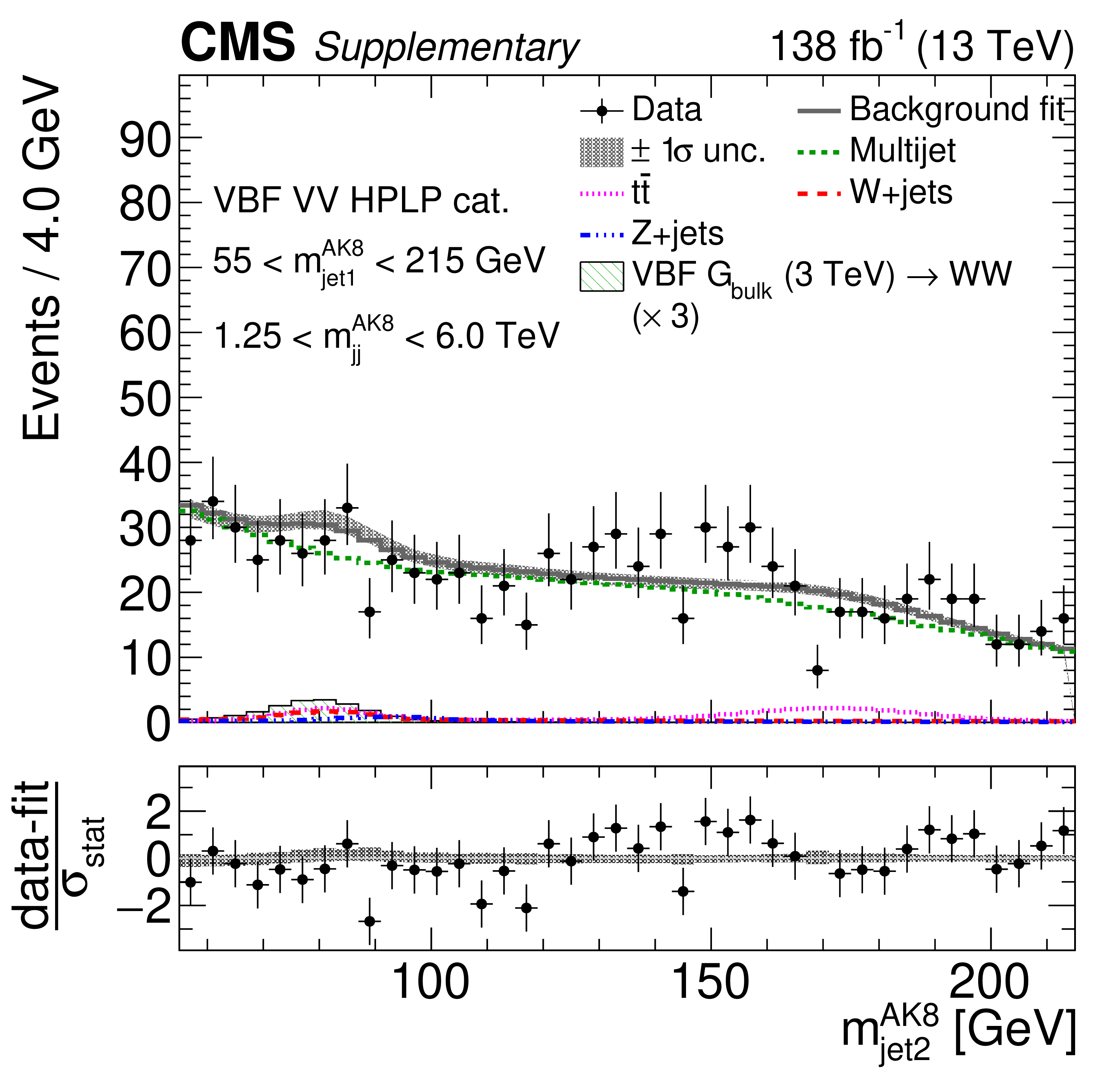
png pdf |
Additional Figure 12-h:
Comparison between the background post-fit and the data distributions of $ m_\text{jet1}^{\mathrm{AK8}} $ (left), $ m_\text{jet2}^{\mathrm{AK8}} $ (middle) and $ m_\mathrm{jj}^{\mathrm{AK8}} $ (right) in the VBF VH LPHP (upper), VBF VH HPLP (middle), and VBF VV HPLP (lower) categories. The background shape uncertainty is shown as a gray shaded band around the result of the maximum likelihood fit to the data under the background-only assumption (gray solid line), and the statistical uncertainties in the data are shown as vertical bars. The various background components contributing to the total background fit are also shown with different line colors. An example of a signal distribution is overlaid, where the number of expected events is scaled by an arbitrary normalization factor. Shown below each mass plot is the difference between the data and the fit divided by the statistical uncertainty in the data; the uncertainty bar represents the statistical uncertainty only. The total uncertainty in the background estimate fitted to the data divided by the statistical uncertainty in the data is shown as a band. |

png pdf |
Additional Figure 12-i:
Comparison between the background post-fit and the data distributions of $ m_\text{jet1}^{\mathrm{AK8}} $ (left), $ m_\text{jet2}^{\mathrm{AK8}} $ (middle) and $ m_\mathrm{jj}^{\mathrm{AK8}} $ (right) in the VBF VH LPHP (upper), VBF VH HPLP (middle), and VBF VV HPLP (lower) categories. The background shape uncertainty is shown as a gray shaded band around the result of the maximum likelihood fit to the data under the background-only assumption (gray solid line), and the statistical uncertainties in the data are shown as vertical bars. The various background components contributing to the total background fit are also shown with different line colors. An example of a signal distribution is overlaid, where the number of expected events is scaled by an arbitrary normalization factor. Shown below each mass plot is the difference between the data and the fit divided by the statistical uncertainty in the data; the uncertainty bar represents the statistical uncertainty only. The total uncertainty in the background estimate fitted to the data divided by the statistical uncertainty in the data is shown as a band. |

png pdf |
Additional Figure 13:
Projections of data and background post-fit distributions onto the $ m_\mathrm{jj}^{\mathrm{AK8}} $ dimension in regions enriched in signal from DY/ggF VV (65 $ < m_\text{jet1}^{\mathrm{AK8}} < $ 105 GeV, 65 $ < m_\text{jet2}^{\mathrm{AK8}} < $ 105 GeV) for the VH LPHP (left), VH HPLP (middle), and VV HPLP DY/ggF categories. The background shape uncertainty is shown as a gray shaded band around the result of the maximum likelihood fit to the data under the background-only assumption (gray solid line), and the statistical uncertainties in the data are shown as vertical bars. The various background components contributing to the total background fit are also shown with different line colors. Shown below each mass plot is the difference between the data and the fit divided by the statistical uncertainty in the data; the uncertainty bar represents the statistical uncertainty only. The total uncertainty in the background estimate fitted to the data divided by the statistical uncertainty in the data is shown as a band. |

png pdf |
Additional Figure 13-a:
Projections of data and background post-fit distributions onto the $ m_\mathrm{jj}^{\mathrm{AK8}} $ dimension in regions enriched in signal from DY/ggF VV (65 $ < m_\text{jet1}^{\mathrm{AK8}} < $ 105 GeV, 65 $ < m_\text{jet2}^{\mathrm{AK8}} < $ 105 GeV) for the VH LPHP (left), VH HPLP (middle), and VV HPLP DY/ggF categories. The background shape uncertainty is shown as a gray shaded band around the result of the maximum likelihood fit to the data under the background-only assumption (gray solid line), and the statistical uncertainties in the data are shown as vertical bars. The various background components contributing to the total background fit are also shown with different line colors. Shown below each mass plot is the difference between the data and the fit divided by the statistical uncertainty in the data; the uncertainty bar represents the statistical uncertainty only. The total uncertainty in the background estimate fitted to the data divided by the statistical uncertainty in the data is shown as a band. |

png pdf |
Additional Figure 13-b:
Projections of data and background post-fit distributions onto the $ m_\mathrm{jj}^{\mathrm{AK8}} $ dimension in regions enriched in signal from DY/ggF VV (65 $ < m_\text{jet1}^{\mathrm{AK8}} < $ 105 GeV, 65 $ < m_\text{jet2}^{\mathrm{AK8}} < $ 105 GeV) for the VH LPHP (left), VH HPLP (middle), and VV HPLP DY/ggF categories. The background shape uncertainty is shown as a gray shaded band around the result of the maximum likelihood fit to the data under the background-only assumption (gray solid line), and the statistical uncertainties in the data are shown as vertical bars. The various background components contributing to the total background fit are also shown with different line colors. Shown below each mass plot is the difference between the data and the fit divided by the statistical uncertainty in the data; the uncertainty bar represents the statistical uncertainty only. The total uncertainty in the background estimate fitted to the data divided by the statistical uncertainty in the data is shown as a band. |

png pdf |
Additional Figure 13-c:
Projections of data and background post-fit distributions onto the $ m_\mathrm{jj}^{\mathrm{AK8}} $ dimension in regions enriched in signal from DY/ggF VV (65 $ < m_\text{jet1}^{\mathrm{AK8}} < $ 105 GeV, 65 $ < m_\text{jet2}^{\mathrm{AK8}} < $ 105 GeV) for the VH LPHP (left), VH HPLP (middle), and VV HPLP DY/ggF categories. The background shape uncertainty is shown as a gray shaded band around the result of the maximum likelihood fit to the data under the background-only assumption (gray solid line), and the statistical uncertainties in the data are shown as vertical bars. The various background components contributing to the total background fit are also shown with different line colors. Shown below each mass plot is the difference between the data and the fit divided by the statistical uncertainty in the data; the uncertainty bar represents the statistical uncertainty only. The total uncertainty in the background estimate fitted to the data divided by the statistical uncertainty in the data is shown as a band. |

png pdf |
Additional Figure 14:
Projections of data and background post-fit distributions onto the $ m_\mathrm{jj}^{\mathrm{AK8}} $ dimension in regions enriched in signal from DY/ggF VH (65 $ < m_\text{jet1/2}^{\mathrm{AK8}} < $ 105 GeV, 110 $ < m_\text{jet2/1}^{\mathrm{AK8}} < $ 140 GeV) for the HPHP (upper) and HPLP/LPHP (lower) DY/ggF categories. The background shape uncertainty is shown as a gray shaded band around the result of the maximum likelihood fit to the data under the background-only assumption (gray solid line), and the statistical uncertainties in the data are shown as vertical bars. The various background components contributing to the total background fit are also shown with different line colors. Shown below each mass plot is the difference between the data and the fit divided by the statistical uncertainty in the data; the uncertainty bar represents the statistical uncertainty only. The total uncertainty in the background estimate fitted to the data divided by the statistical uncertainty in the data is shown as a band. |
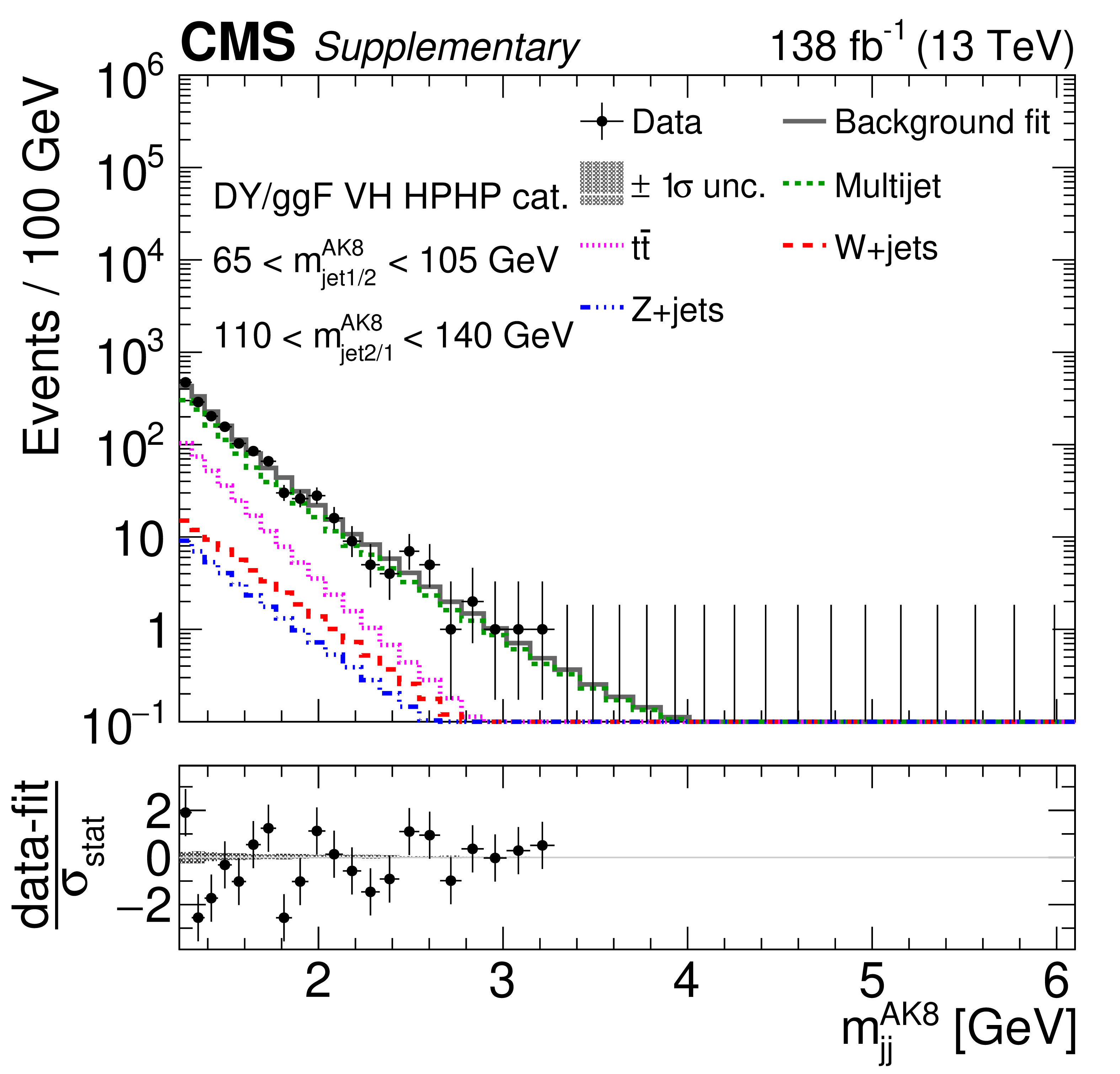
png pdf |
Additional Figure 14-a:
Projections of data and background post-fit distributions onto the $ m_\mathrm{jj}^{\mathrm{AK8}} $ dimension in regions enriched in signal from DY/ggF VH (65 $ < m_\text{jet1/2}^{\mathrm{AK8}} < $ 105 GeV, 110 $ < m_\text{jet2/1}^{\mathrm{AK8}} < $ 140 GeV) for the HPHP (upper) and HPLP/LPHP (lower) DY/ggF categories. The background shape uncertainty is shown as a gray shaded band around the result of the maximum likelihood fit to the data under the background-only assumption (gray solid line), and the statistical uncertainties in the data are shown as vertical bars. The various background components contributing to the total background fit are also shown with different line colors. Shown below each mass plot is the difference between the data and the fit divided by the statistical uncertainty in the data; the uncertainty bar represents the statistical uncertainty only. The total uncertainty in the background estimate fitted to the data divided by the statistical uncertainty in the data is shown as a band. |

png pdf |
Additional Figure 14-b:
Projections of data and background post-fit distributions onto the $ m_\mathrm{jj}^{\mathrm{AK8}} $ dimension in regions enriched in signal from DY/ggF VH (65 $ < m_\text{jet1/2}^{\mathrm{AK8}} < $ 105 GeV, 110 $ < m_\text{jet2/1}^{\mathrm{AK8}} < $ 140 GeV) for the HPHP (upper) and HPLP/LPHP (lower) DY/ggF categories. The background shape uncertainty is shown as a gray shaded band around the result of the maximum likelihood fit to the data under the background-only assumption (gray solid line), and the statistical uncertainties in the data are shown as vertical bars. The various background components contributing to the total background fit are also shown with different line colors. Shown below each mass plot is the difference between the data and the fit divided by the statistical uncertainty in the data; the uncertainty bar represents the statistical uncertainty only. The total uncertainty in the background estimate fitted to the data divided by the statistical uncertainty in the data is shown as a band. |

png pdf |
Additional Figure 14-c:
Projections of data and background post-fit distributions onto the $ m_\mathrm{jj}^{\mathrm{AK8}} $ dimension in regions enriched in signal from DY/ggF VH (65 $ < m_\text{jet1/2}^{\mathrm{AK8}} < $ 105 GeV, 110 $ < m_\text{jet2/1}^{\mathrm{AK8}} < $ 140 GeV) for the HPHP (upper) and HPLP/LPHP (lower) DY/ggF categories. The background shape uncertainty is shown as a gray shaded band around the result of the maximum likelihood fit to the data under the background-only assumption (gray solid line), and the statistical uncertainties in the data are shown as vertical bars. The various background components contributing to the total background fit are also shown with different line colors. Shown below each mass plot is the difference between the data and the fit divided by the statistical uncertainty in the data; the uncertainty bar represents the statistical uncertainty only. The total uncertainty in the background estimate fitted to the data divided by the statistical uncertainty in the data is shown as a band. |

png pdf |
Additional Figure 14-d:
Projections of data and background post-fit distributions onto the $ m_\mathrm{jj}^{\mathrm{AK8}} $ dimension in regions enriched in signal from DY/ggF VH (65 $ < m_\text{jet1/2}^{\mathrm{AK8}} < $ 105 GeV, 110 $ < m_\text{jet2/1}^{\mathrm{AK8}} < $ 140 GeV) for the HPHP (upper) and HPLP/LPHP (lower) DY/ggF categories. The background shape uncertainty is shown as a gray shaded band around the result of the maximum likelihood fit to the data under the background-only assumption (gray solid line), and the statistical uncertainties in the data are shown as vertical bars. The various background components contributing to the total background fit are also shown with different line colors. Shown below each mass plot is the difference between the data and the fit divided by the statistical uncertainty in the data; the uncertainty bar represents the statistical uncertainty only. The total uncertainty in the background estimate fitted to the data divided by the statistical uncertainty in the data is shown as a band. |

png pdf |
Additional Figure 14-e:
Projections of data and background post-fit distributions onto the $ m_\mathrm{jj}^{\mathrm{AK8}} $ dimension in regions enriched in signal from DY/ggF VH (65 $ < m_\text{jet1/2}^{\mathrm{AK8}} < $ 105 GeV, 110 $ < m_\text{jet2/1}^{\mathrm{AK8}} < $ 140 GeV) for the HPHP (upper) and HPLP/LPHP (lower) DY/ggF categories. The background shape uncertainty is shown as a gray shaded band around the result of the maximum likelihood fit to the data under the background-only assumption (gray solid line), and the statistical uncertainties in the data are shown as vertical bars. The various background components contributing to the total background fit are also shown with different line colors. Shown below each mass plot is the difference between the data and the fit divided by the statistical uncertainty in the data; the uncertainty bar represents the statistical uncertainty only. The total uncertainty in the background estimate fitted to the data divided by the statistical uncertainty in the data is shown as a band. |
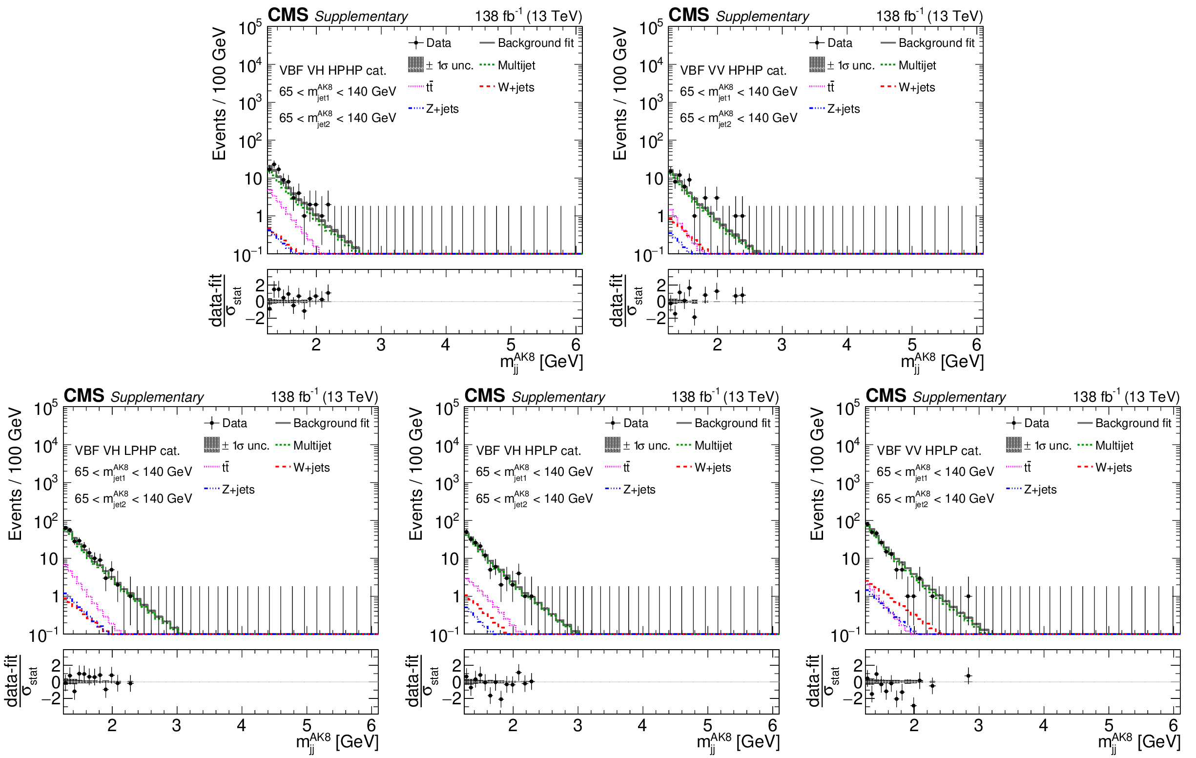
png pdf |
Additional Figure 15:
Projections of data and background post-fit distributions onto the $ m_\mathrm{jj}^{\mathrm{AK8}} $ dimension in regions enriched in signal from VBF VV/VH (65 $ < m_\text{jet1}^{\mathrm{AK8}} < $ 140 GeV, 65 $ < m_\text{jet2}^{\mathrm{AK8}} < $ 140 GeV) for the HPHP (upper) and HPLP/LPHP (lower) VBF categories. The background shape uncertainty is shown as a gray shaded band around the result of the maximum likelihood fit to the data under the background-only assumption (gray solid line), and the statistical uncertainties in the data are shown as vertical bars. The various background components contributing to the total background fit are also shown with different line colors. Shown below each mass plot is the difference between the data and the fit divided by the statistical uncertainty in the data; the uncertainty bar represents the statistical uncertainty only. The total uncertainty in the background estimate fitted to the data divided by the statistical uncertainty in the data is shown as a band. |

png pdf |
Additional Figure 15-a:
Projections of data and background post-fit distributions onto the $ m_\mathrm{jj}^{\mathrm{AK8}} $ dimension in regions enriched in signal from VBF VV/VH (65 $ < m_\text{jet1}^{\mathrm{AK8}} < $ 140 GeV, 65 $ < m_\text{jet2}^{\mathrm{AK8}} < $ 140 GeV) for the HPHP (upper) and HPLP/LPHP (lower) VBF categories. The background shape uncertainty is shown as a gray shaded band around the result of the maximum likelihood fit to the data under the background-only assumption (gray solid line), and the statistical uncertainties in the data are shown as vertical bars. The various background components contributing to the total background fit are also shown with different line colors. Shown below each mass plot is the difference between the data and the fit divided by the statistical uncertainty in the data; the uncertainty bar represents the statistical uncertainty only. The total uncertainty in the background estimate fitted to the data divided by the statistical uncertainty in the data is shown as a band. |

png pdf |
Additional Figure 15-b:
Projections of data and background post-fit distributions onto the $ m_\mathrm{jj}^{\mathrm{AK8}} $ dimension in regions enriched in signal from VBF VV/VH (65 $ < m_\text{jet1}^{\mathrm{AK8}} < $ 140 GeV, 65 $ < m_\text{jet2}^{\mathrm{AK8}} < $ 140 GeV) for the HPHP (upper) and HPLP/LPHP (lower) VBF categories. The background shape uncertainty is shown as a gray shaded band around the result of the maximum likelihood fit to the data under the background-only assumption (gray solid line), and the statistical uncertainties in the data are shown as vertical bars. The various background components contributing to the total background fit are also shown with different line colors. Shown below each mass plot is the difference between the data and the fit divided by the statistical uncertainty in the data; the uncertainty bar represents the statistical uncertainty only. The total uncertainty in the background estimate fitted to the data divided by the statistical uncertainty in the data is shown as a band. |

png pdf |
Additional Figure 15-c:
Projections of data and background post-fit distributions onto the $ m_\mathrm{jj}^{\mathrm{AK8}} $ dimension in regions enriched in signal from VBF VV/VH (65 $ < m_\text{jet1}^{\mathrm{AK8}} < $ 140 GeV, 65 $ < m_\text{jet2}^{\mathrm{AK8}} < $ 140 GeV) for the HPHP (upper) and HPLP/LPHP (lower) VBF categories. The background shape uncertainty is shown as a gray shaded band around the result of the maximum likelihood fit to the data under the background-only assumption (gray solid line), and the statistical uncertainties in the data are shown as vertical bars. The various background components contributing to the total background fit are also shown with different line colors. Shown below each mass plot is the difference between the data and the fit divided by the statistical uncertainty in the data; the uncertainty bar represents the statistical uncertainty only. The total uncertainty in the background estimate fitted to the data divided by the statistical uncertainty in the data is shown as a band. |
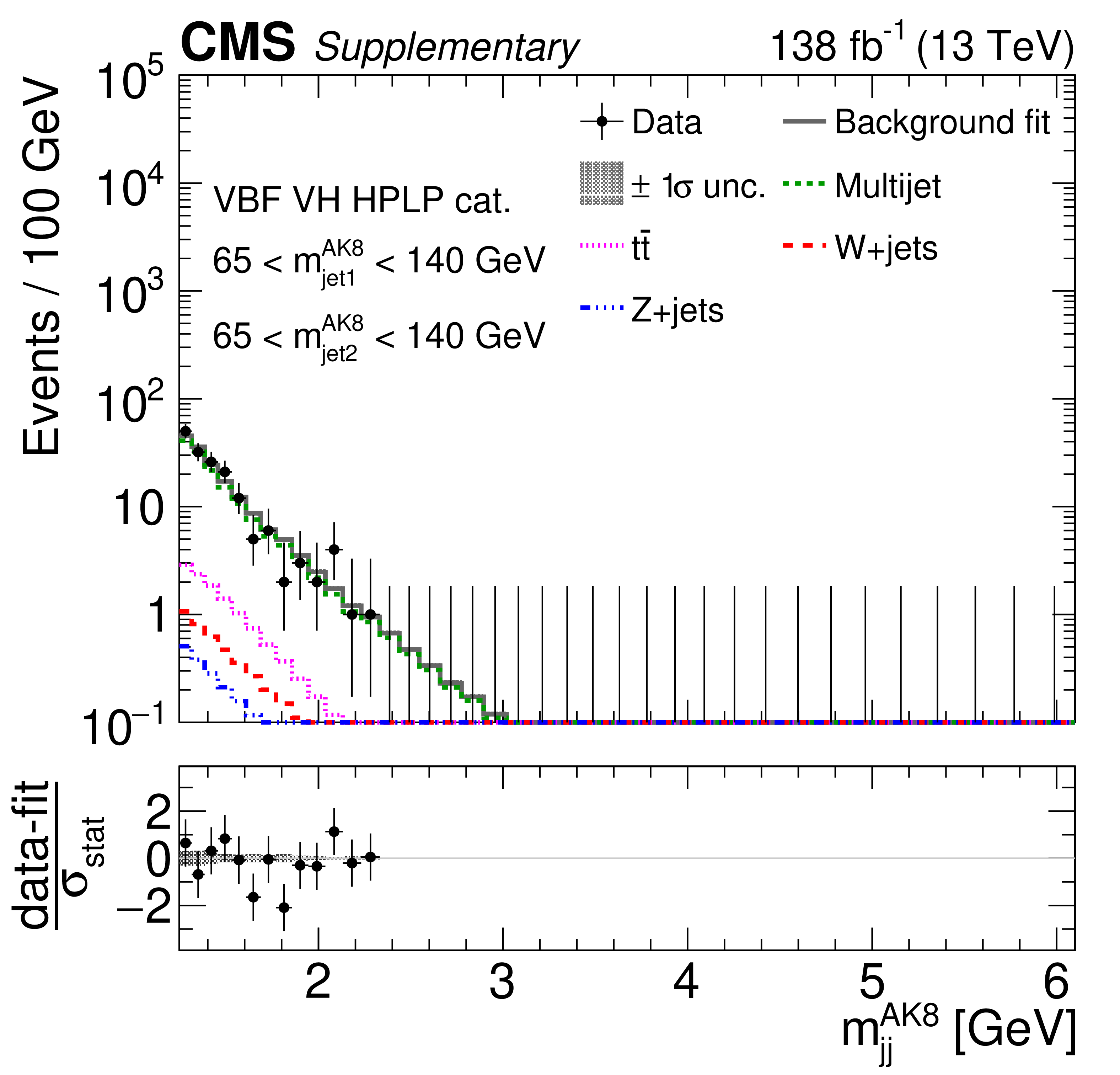
png pdf |
Additional Figure 15-d:
Projections of data and background post-fit distributions onto the $ m_\mathrm{jj}^{\mathrm{AK8}} $ dimension in regions enriched in signal from VBF VV/VH (65 $ < m_\text{jet1}^{\mathrm{AK8}} < $ 140 GeV, 65 $ < m_\text{jet2}^{\mathrm{AK8}} < $ 140 GeV) for the HPHP (upper) and HPLP/LPHP (lower) VBF categories. The background shape uncertainty is shown as a gray shaded band around the result of the maximum likelihood fit to the data under the background-only assumption (gray solid line), and the statistical uncertainties in the data are shown as vertical bars. The various background components contributing to the total background fit are also shown with different line colors. Shown below each mass plot is the difference between the data and the fit divided by the statistical uncertainty in the data; the uncertainty bar represents the statistical uncertainty only. The total uncertainty in the background estimate fitted to the data divided by the statistical uncertainty in the data is shown as a band. |

png pdf |
Additional Figure 15-e:
Projections of data and background post-fit distributions onto the $ m_\mathrm{jj}^{\mathrm{AK8}} $ dimension in regions enriched in signal from VBF VV/VH (65 $ < m_\text{jet1}^{\mathrm{AK8}} < $ 140 GeV, 65 $ < m_\text{jet2}^{\mathrm{AK8}} < $ 140 GeV) for the HPHP (upper) and HPLP/LPHP (lower) VBF categories. The background shape uncertainty is shown as a gray shaded band around the result of the maximum likelihood fit to the data under the background-only assumption (gray solid line), and the statistical uncertainties in the data are shown as vertical bars. The various background components contributing to the total background fit are also shown with different line colors. Shown below each mass plot is the difference between the data and the fit divided by the statistical uncertainty in the data; the uncertainty bar represents the statistical uncertainty only. The total uncertainty in the background estimate fitted to the data divided by the statistical uncertainty in the data is shown as a band. |

png pdf |
Additional Figure 16:
Projection of the 3D phase space of the data onto the $ m_\mathrm{jj}^{\mathrm{AK8}} $--$ m_\text{jet1}^{\mathrm{AK8}} $ plane for a selected region in $ m_\text{jet2}^{\mathrm{AK8}} $ enriched in signal from DY/ggF VV. Contours of the signal and background distributions after the background post-fit are overlaid. The projections are shown for the HPHP VH (VV) DY/ggF category on the left (right). |

png pdf |
Additional Figure 16-a:
Projection of the 3D phase space of the data onto the $ m_\mathrm{jj}^{\mathrm{AK8}} $--$ m_\text{jet1}^{\mathrm{AK8}} $ plane for a selected region in $ m_\text{jet2}^{\mathrm{AK8}} $ enriched in signal from DY/ggF VV. Contours of the signal and background distributions after the background post-fit are overlaid. The projections are shown for the HPHP VH (VV) DY/ggF category on the left (right). |

png pdf |
Additional Figure 16-b:
Projection of the 3D phase space of the data onto the $ m_\mathrm{jj}^{\mathrm{AK8}} $--$ m_\text{jet1}^{\mathrm{AK8}} $ plane for a selected region in $ m_\text{jet2}^{\mathrm{AK8}} $ enriched in signal from DY/ggF VV. Contours of the signal and background distributions after the background post-fit are overlaid. The projections are shown for the HPHP VH (VV) DY/ggF category on the left (right). |
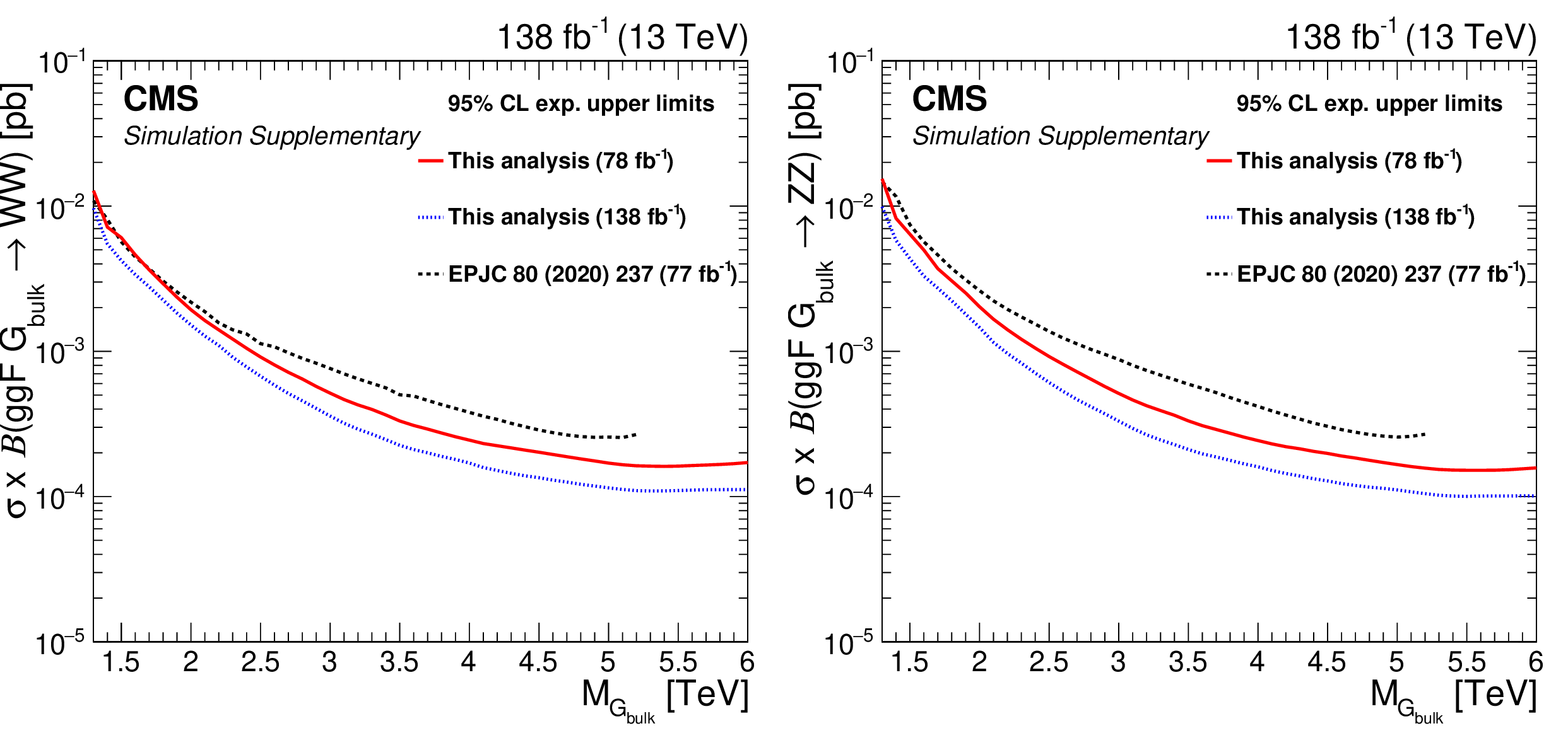
png pdf |
Additional Figure 17:
Expected 95% CL\ upper limits on the product of the production cross section ($ \sigma $) and the branching fraction for a $ \mathrm{G}_{\text{bulk}}\to\mathrm{W}\mathrm{W} $ (left) and a $ \mathrm{G}_{\text{bulk}}\to\mathrm{Z}\mathrm{Z} $ (right) signal using 77.3 fb$ ^{-1} $ of data collected in 2016+2017 obtained using the methods presented here (red solid line), compared to the result obtained with previous methods (black dash-dotted line), published in EPJC 80 (2020) 237. The limit obtained combining data collected in 2016--2018 in this paper is also shown (blue dashed line). |

png pdf |
Additional Figure 17-a:
Expected 95% CL\ upper limits on the product of the production cross section ($ \sigma $) and the branching fraction for a $ \mathrm{G}_{\text{bulk}}\to\mathrm{W}\mathrm{W} $ (left) and a $ \mathrm{G}_{\text{bulk}}\to\mathrm{Z}\mathrm{Z} $ (right) signal using 77.3 fb$ ^{-1} $ of data collected in 2016+2017 obtained using the methods presented here (red solid line), compared to the result obtained with previous methods (black dash-dotted line), published in EPJC 80 (2020) 237. The limit obtained combining data collected in 2016--2018 in this paper is also shown (blue dashed line). |

png pdf |
Additional Figure 17-b:
Expected 95% CL\ upper limits on the product of the production cross section ($ \sigma $) and the branching fraction for a $ \mathrm{G}_{\text{bulk}}\to\mathrm{W}\mathrm{W} $ (left) and a $ \mathrm{G}_{\text{bulk}}\to\mathrm{Z}\mathrm{Z} $ (right) signal using 77.3 fb$ ^{-1} $ of data collected in 2016+2017 obtained using the methods presented here (red solid line), compared to the result obtained with previous methods (black dash-dotted line), published in EPJC 80 (2020) 237. The limit obtained combining data collected in 2016--2018 in this paper is also shown (blue dashed line). |

png pdf |
Additional Figure 18:
Observed and expected 95% CL\ upper limits on the product of the production cross section ($ \sigma $) and the branching fraction, obtained after combining all categories with 138 fb$^{-1}$ fb$ ^{-1} $ of data at $ \sqrt{s}= $ 13 TeV, for $ \mathrm{G}_{\text{bulk}}\to\mathrm{W}\mathrm{W} $ (left) and $ \mathrm{G}_{\text{bulk}}\to\mathrm{Z}\mathrm{Z} $ (right) signals. In the upper panel the ggF production mode is shown while in the lower panel the VBF mode is presented. For each signal scenario the theoretical prediction (red line) and its uncertainty associated with the choice of PDF set (red hashed band) is shown. |

png pdf |
Additional Figure 18-a:
Observed and expected 95% CL\ upper limits on the product of the production cross section ($ \sigma $) and the branching fraction, obtained after combining all categories with 138 fb$^{-1}$ fb$ ^{-1} $ of data at $ \sqrt{s}= $ 13 TeV, for $ \mathrm{G}_{\text{bulk}}\to\mathrm{W}\mathrm{W} $ (left) and $ \mathrm{G}_{\text{bulk}}\to\mathrm{Z}\mathrm{Z} $ (right) signals. In the upper panel the ggF production mode is shown while in the lower panel the VBF mode is presented. For each signal scenario the theoretical prediction (red line) and its uncertainty associated with the choice of PDF set (red hashed band) is shown. |

png pdf |
Additional Figure 18-b:
Observed and expected 95% CL\ upper limits on the product of the production cross section ($ \sigma $) and the branching fraction, obtained after combining all categories with 138 fb$^{-1}$ fb$ ^{-1} $ of data at $ \sqrt{s}= $ 13 TeV, for $ \mathrm{G}_{\text{bulk}}\to\mathrm{W}\mathrm{W} $ (left) and $ \mathrm{G}_{\text{bulk}}\to\mathrm{Z}\mathrm{Z} $ (right) signals. In the upper panel the ggF production mode is shown while in the lower panel the VBF mode is presented. For each signal scenario the theoretical prediction (red line) and its uncertainty associated with the choice of PDF set (red hashed band) is shown. |

png pdf |
Additional Figure 18-c:
Observed and expected 95% CL\ upper limits on the product of the production cross section ($ \sigma $) and the branching fraction, obtained after combining all categories with 138 fb$^{-1}$ fb$ ^{-1} $ of data at $ \sqrt{s}= $ 13 TeV, for $ \mathrm{G}_{\text{bulk}}\to\mathrm{W}\mathrm{W} $ (left) and $ \mathrm{G}_{\text{bulk}}\to\mathrm{Z}\mathrm{Z} $ (right) signals. In the upper panel the ggF production mode is shown while in the lower panel the VBF mode is presented. For each signal scenario the theoretical prediction (red line) and its uncertainty associated with the choice of PDF set (red hashed band) is shown. |

png pdf |
Additional Figure 18-d:
Observed and expected 95% CL\ upper limits on the product of the production cross section ($ \sigma $) and the branching fraction, obtained after combining all categories with 138 fb$^{-1}$ fb$ ^{-1} $ of data at $ \sqrt{s}= $ 13 TeV, for $ \mathrm{G}_{\text{bulk}}\to\mathrm{W}\mathrm{W} $ (left) and $ \mathrm{G}_{\text{bulk}}\to\mathrm{Z}\mathrm{Z} $ (right) signals. In the upper panel the ggF production mode is shown while in the lower panel the VBF mode is presented. For each signal scenario the theoretical prediction (red line) and its uncertainty associated with the choice of PDF set (red hashed band) is shown. |

png pdf |
Additional Figure 19:
Observed and expected 95% CL\ upper limits on the product of the production cross section ($ \sigma $) and the branching fraction, obtained after combining all categories with 138 fb$^{-1}$ fb$ ^{-1} $ of data at $ \sqrt{s}= $ 13 TeV, for $ \text{Rad} \to\mathrm{W}\mathrm{W} $ (left) and $ \text{Rad} \to\mathrm{Z}\mathrm{Z} $ (right) signals. In the upper panel the ggF production mode is shown while in the lower panel the VBF mode is presented. For each signal scenario the theoretical prediction (red line) and its uncertainty associated with the choice of PDF set (red hashed band) is shown. |

png pdf |
Additional Figure 19-a:
Observed and expected 95% CL\ upper limits on the product of the production cross section ($ \sigma $) and the branching fraction, obtained after combining all categories with 138 fb$^{-1}$ fb$ ^{-1} $ of data at $ \sqrt{s}= $ 13 TeV, for $ \text{Rad} \to\mathrm{W}\mathrm{W} $ (left) and $ \text{Rad} \to\mathrm{Z}\mathrm{Z} $ (right) signals. In the upper panel the ggF production mode is shown while in the lower panel the VBF mode is presented. For each signal scenario the theoretical prediction (red line) and its uncertainty associated with the choice of PDF set (red hashed band) is shown. |
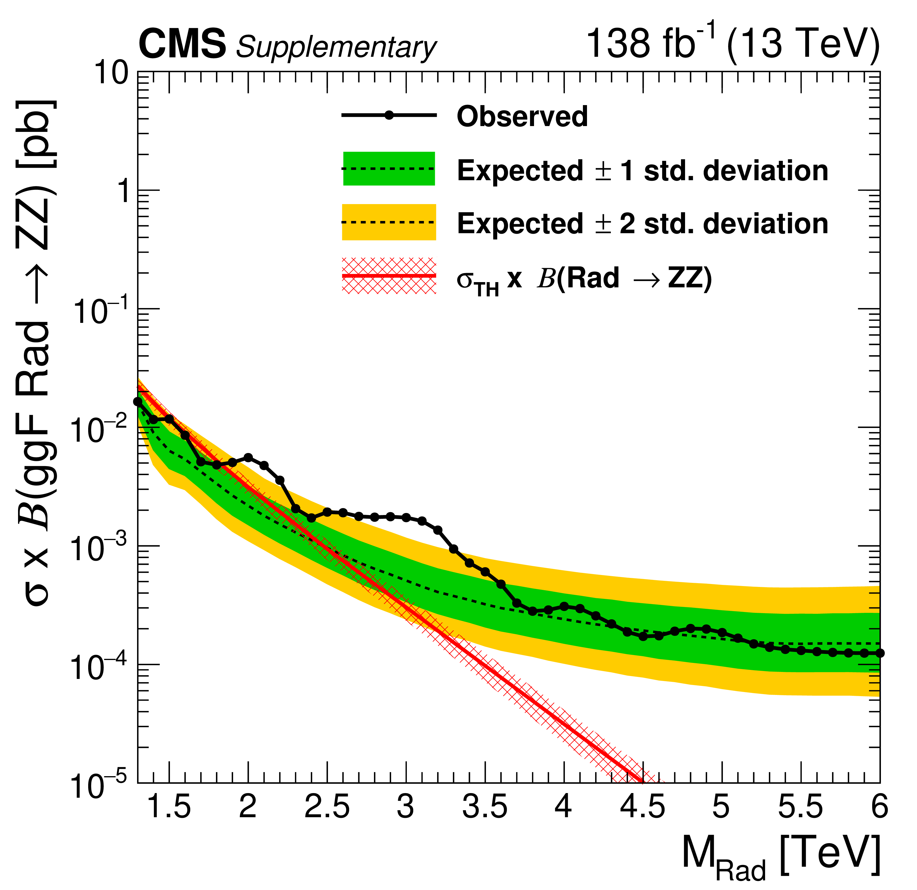
png pdf |
Additional Figure 19-b:
Observed and expected 95% CL\ upper limits on the product of the production cross section ($ \sigma $) and the branching fraction, obtained after combining all categories with 138 fb$^{-1}$ fb$ ^{-1} $ of data at $ \sqrt{s}= $ 13 TeV, for $ \text{Rad} \to\mathrm{W}\mathrm{W} $ (left) and $ \text{Rad} \to\mathrm{Z}\mathrm{Z} $ (right) signals. In the upper panel the ggF production mode is shown while in the lower panel the VBF mode is presented. For each signal scenario the theoretical prediction (red line) and its uncertainty associated with the choice of PDF set (red hashed band) is shown. |

png pdf |
Additional Figure 19-c:
Observed and expected 95% CL\ upper limits on the product of the production cross section ($ \sigma $) and the branching fraction, obtained after combining all categories with 138 fb$^{-1}$ fb$ ^{-1} $ of data at $ \sqrt{s}= $ 13 TeV, for $ \text{Rad} \to\mathrm{W}\mathrm{W} $ (left) and $ \text{Rad} \to\mathrm{Z}\mathrm{Z} $ (right) signals. In the upper panel the ggF production mode is shown while in the lower panel the VBF mode is presented. For each signal scenario the theoretical prediction (red line) and its uncertainty associated with the choice of PDF set (red hashed band) is shown. |

png pdf |
Additional Figure 19-d:
Observed and expected 95% CL\ upper limits on the product of the production cross section ($ \sigma $) and the branching fraction, obtained after combining all categories with 138 fb$^{-1}$ fb$ ^{-1} $ of data at $ \sqrt{s}= $ 13 TeV, for $ \text{Rad} \to\mathrm{W}\mathrm{W} $ (left) and $ \text{Rad} \to\mathrm{Z}\mathrm{Z} $ (right) signals. In the upper panel the ggF production mode is shown while in the lower panel the VBF mode is presented. For each signal scenario the theoretical prediction (red line) and its uncertainty associated with the choice of PDF set (red hashed band) is shown. |

png pdf |
Additional Figure 20:
Observed and expected 95% CL\ upper limits on the product of the production cross section ($ \sigma $) and the branching fraction, obtained after combining all categories with 138 fb$^{-1}$ fb$ ^{-1} $ of data at $ \sqrt{s}= $ 13 TeV, for $ \mathrm{Z}^{'}\to\mathrm{W}\mathrm{W} $ (left) and $ \mathrm{W^{'}}\to\mathrm{W}\mathrm{Z} $ (right) signals. In the upper panel the DY production mode is shown while in the lower panel the VBF mode is presented. For each signal scenario the theoretical prediction (red line for $ c_{\mathrm{H}} = $ 1, blue line for $ c_{\mathrm{H}} = $ 3) and its uncertainty associated with the choice of PDF set (red and blue hashed bands) is shown. |
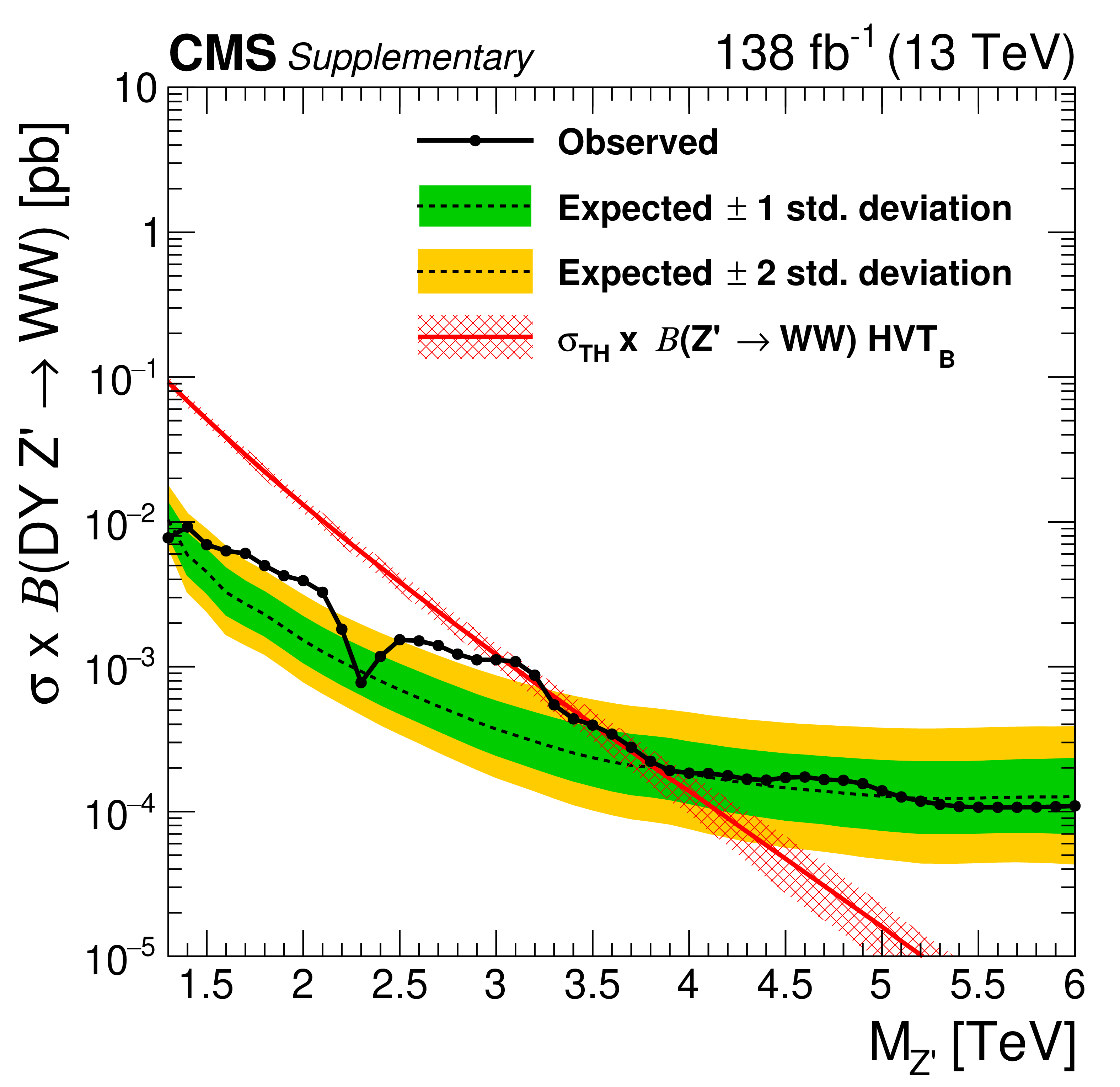
png pdf |
Additional Figure 20-a:
Observed and expected 95% CL\ upper limits on the product of the production cross section ($ \sigma $) and the branching fraction, obtained after combining all categories with 138 fb$^{-1}$ fb$ ^{-1} $ of data at $ \sqrt{s}= $ 13 TeV, for $ \mathrm{Z}^{'}\to\mathrm{W}\mathrm{W} $ (left) and $ \mathrm{W^{'}}\to\mathrm{W}\mathrm{Z} $ (right) signals. In the upper panel the DY production mode is shown while in the lower panel the VBF mode is presented. For each signal scenario the theoretical prediction (red line for $ c_{\mathrm{H}} = $ 1, blue line for $ c_{\mathrm{H}} = $ 3) and its uncertainty associated with the choice of PDF set (red and blue hashed bands) is shown. |

png pdf |
Additional Figure 20-b:
Observed and expected 95% CL\ upper limits on the product of the production cross section ($ \sigma $) and the branching fraction, obtained after combining all categories with 138 fb$^{-1}$ fb$ ^{-1} $ of data at $ \sqrt{s}= $ 13 TeV, for $ \mathrm{Z}^{'}\to\mathrm{W}\mathrm{W} $ (left) and $ \mathrm{W^{'}}\to\mathrm{W}\mathrm{Z} $ (right) signals. In the upper panel the DY production mode is shown while in the lower panel the VBF mode is presented. For each signal scenario the theoretical prediction (red line for $ c_{\mathrm{H}} = $ 1, blue line for $ c_{\mathrm{H}} = $ 3) and its uncertainty associated with the choice of PDF set (red and blue hashed bands) is shown. |

png pdf |
Additional Figure 20-c:
Observed and expected 95% CL\ upper limits on the product of the production cross section ($ \sigma $) and the branching fraction, obtained after combining all categories with 138 fb$^{-1}$ fb$ ^{-1} $ of data at $ \sqrt{s}= $ 13 TeV, for $ \mathrm{Z}^{'}\to\mathrm{W}\mathrm{W} $ (left) and $ \mathrm{W^{'}}\to\mathrm{W}\mathrm{Z} $ (right) signals. In the upper panel the DY production mode is shown while in the lower panel the VBF mode is presented. For each signal scenario the theoretical prediction (red line for $ c_{\mathrm{H}} = $ 1, blue line for $ c_{\mathrm{H}} = $ 3) and its uncertainty associated with the choice of PDF set (red and blue hashed bands) is shown. |

png pdf |
Additional Figure 20-d:
Observed and expected 95% CL\ upper limits on the product of the production cross section ($ \sigma $) and the branching fraction, obtained after combining all categories with 138 fb$^{-1}$ fb$ ^{-1} $ of data at $ \sqrt{s}= $ 13 TeV, for $ \mathrm{Z}^{'}\to\mathrm{W}\mathrm{W} $ (left) and $ \mathrm{W^{'}}\to\mathrm{W}\mathrm{Z} $ (right) signals. In the upper panel the DY production mode is shown while in the lower panel the VBF mode is presented. For each signal scenario the theoretical prediction (red line for $ c_{\mathrm{H}} = $ 1, blue line for $ c_{\mathrm{H}} = $ 3) and its uncertainty associated with the choice of PDF set (red and blue hashed bands) is shown. |

png pdf |
Additional Figure 21:
Observed and expected 95% CL\ upper limits on the product of the production cross section ($ \sigma $) and the branching fraction, obtained after combining all categories with 138 fb$^{-1}$ fb$ ^{-1} $ of data at $ \sqrt{s}= $ 13 TeV, for $ \mathrm{Z}^{'}\to\mathrm{Z}\mathrm{H} $ (left) and $ \mathrm{W^{'}}\to\mathrm{W}\mathrm{H} $ (right) signals. In the upper panel the DY production mode is shown while in the lower panel the VBF mode is presented. For each signal scenario the theoretical prediction (red line for $ c_{\mathrm{H}} = $ 1, blue line for $ c_{\mathrm{H}} = $ 3) and its uncertainty associated with the choice of PDF set (red and blue hashed bands) is shown. |

png pdf |
Additional Figure 21-a:
Observed and expected 95% CL\ upper limits on the product of the production cross section ($ \sigma $) and the branching fraction, obtained after combining all categories with 138 fb$^{-1}$ fb$ ^{-1} $ of data at $ \sqrt{s}= $ 13 TeV, for $ \mathrm{Z}^{'}\to\mathrm{Z}\mathrm{H} $ (left) and $ \mathrm{W^{'}}\to\mathrm{W}\mathrm{H} $ (right) signals. In the upper panel the DY production mode is shown while in the lower panel the VBF mode is presented. For each signal scenario the theoretical prediction (red line for $ c_{\mathrm{H}} = $ 1, blue line for $ c_{\mathrm{H}} = $ 3) and its uncertainty associated with the choice of PDF set (red and blue hashed bands) is shown. |
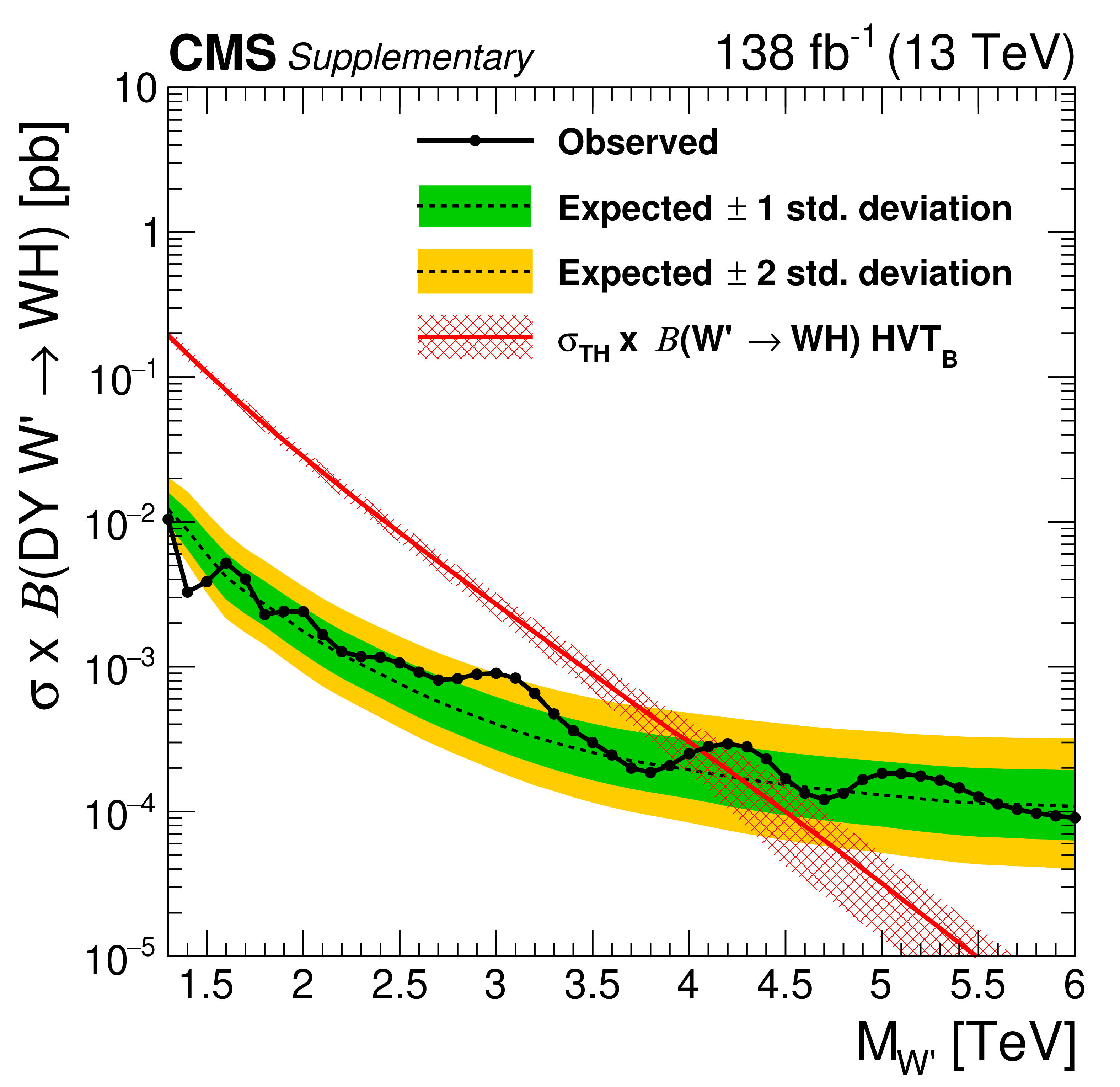
png pdf |
Additional Figure 21-b:
Observed and expected 95% CL\ upper limits on the product of the production cross section ($ \sigma $) and the branching fraction, obtained after combining all categories with 138 fb$^{-1}$ fb$ ^{-1} $ of data at $ \sqrt{s}= $ 13 TeV, for $ \mathrm{Z}^{'}\to\mathrm{Z}\mathrm{H} $ (left) and $ \mathrm{W^{'}}\to\mathrm{W}\mathrm{H} $ (right) signals. In the upper panel the DY production mode is shown while in the lower panel the VBF mode is presented. For each signal scenario the theoretical prediction (red line for $ c_{\mathrm{H}} = $ 1, blue line for $ c_{\mathrm{H}} = $ 3) and its uncertainty associated with the choice of PDF set (red and blue hashed bands) is shown. |

png pdf |
Additional Figure 21-c:
Observed and expected 95% CL\ upper limits on the product of the production cross section ($ \sigma $) and the branching fraction, obtained after combining all categories with 138 fb$^{-1}$ fb$ ^{-1} $ of data at $ \sqrt{s}= $ 13 TeV, for $ \mathrm{Z}^{'}\to\mathrm{Z}\mathrm{H} $ (left) and $ \mathrm{W^{'}}\to\mathrm{W}\mathrm{H} $ (right) signals. In the upper panel the DY production mode is shown while in the lower panel the VBF mode is presented. For each signal scenario the theoretical prediction (red line for $ c_{\mathrm{H}} = $ 1, blue line for $ c_{\mathrm{H}} = $ 3) and its uncertainty associated with the choice of PDF set (red and blue hashed bands) is shown. |
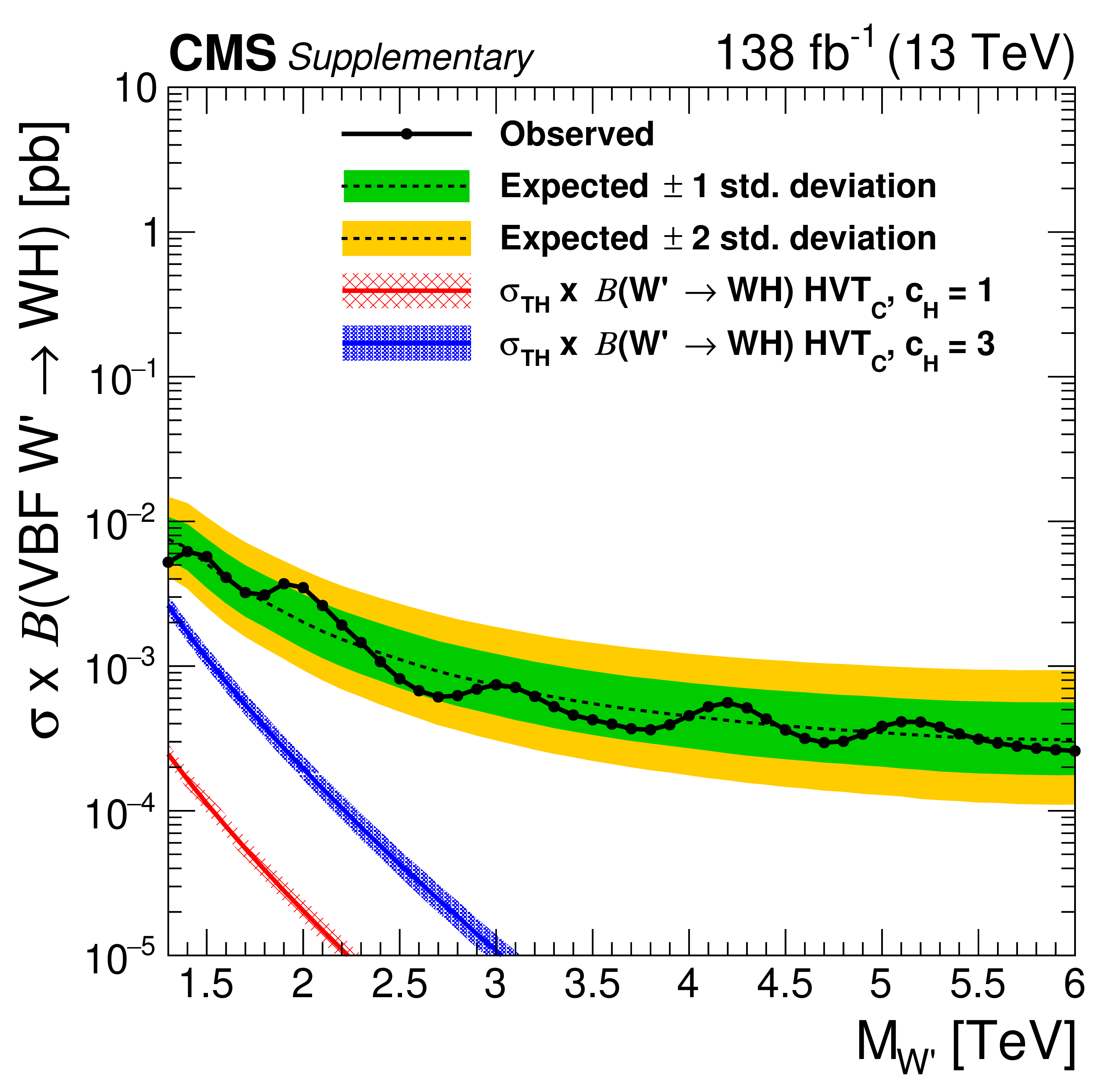
png pdf |
Additional Figure 21-d:
Observed and expected 95% CL\ upper limits on the product of the production cross section ($ \sigma $) and the branching fraction, obtained after combining all categories with 138 fb$^{-1}$ fb$ ^{-1} $ of data at $ \sqrt{s}= $ 13 TeV, for $ \mathrm{Z}^{'}\to\mathrm{Z}\mathrm{H} $ (left) and $ \mathrm{W^{'}}\to\mathrm{W}\mathrm{H} $ (right) signals. In the upper panel the DY production mode is shown while in the lower panel the VBF mode is presented. For each signal scenario the theoretical prediction (red line for $ c_{\mathrm{H}} = $ 1, blue line for $ c_{\mathrm{H}} = $ 3) and its uncertainty associated with the choice of PDF set (red and blue hashed bands) is shown. |

png pdf |
Additional Figure 22:
Observed and expected 95% CL\ upper limits on the product of the production cross section ($ \sigma $) and the branching fraction, obtained after combining all categories with 138 fb$^{-1}$ fb$ ^{-1} $ of data at $ \sqrt{s}= $ 13 TeV, for VBF produced $ \text{Rad} \to\mathrm{V}\mathrm{V} $ (left) and $ \mathrm{G}_{\text{bulk}}\to\mathrm{V}\mathrm{V} $ (right) signals. For each signal scenario the theoretical prediction (red line) and its uncertainty associated with the choice of PDF set (red hashed band) is shown. |

png pdf |
Additional Figure 22-a:
Observed and expected 95% CL\ upper limits on the product of the production cross section ($ \sigma $) and the branching fraction, obtained after combining all categories with 138 fb$^{-1}$ fb$ ^{-1} $ of data at $ \sqrt{s}= $ 13 TeV, for VBF produced $ \text{Rad} \to\mathrm{V}\mathrm{V} $ (left) and $ \mathrm{G}_{\text{bulk}}\to\mathrm{V}\mathrm{V} $ (right) signals. For each signal scenario the theoretical prediction (red line) and its uncertainty associated with the choice of PDF set (red hashed band) is shown. |

png pdf |
Additional Figure 22-b:
Observed and expected 95% CL\ upper limits on the product of the production cross section ($ \sigma $) and the branching fraction, obtained after combining all categories with 138 fb$^{-1}$ fb$ ^{-1} $ of data at $ \sqrt{s}= $ 13 TeV, for VBF produced $ \text{Rad} \to\mathrm{V}\mathrm{V} $ (left) and $ \mathrm{G}_{\text{bulk}}\to\mathrm{V}\mathrm{V} $ (right) signals. For each signal scenario the theoretical prediction (red line) and its uncertainty associated with the choice of PDF set (red hashed band) is shown. |

png pdf |
Additional Figure 23:
Observed and expected 95% CL\ upper limits on the product of the production cross section ($ \sigma $) and the branching fraction, obtained after combining all categories with 138 fb$^{-1}$ fb$ ^{-1} $ of data at $ \sqrt{s}= $ 13 TeV, for $ \mathrm{V}^\prime\to\mathrm{W}\mathrm{V} $ (upper) and $ \mathrm{V}^\prime\to\mathrm{V}\mathrm{H} $ (lower) signals. In the upper panel the DY production mode is shown while in the lower panel the VBF mode is presented. For each signal scenario the theoretical prediction (red line for $ c_{\mathrm{H}} = $ 1, blue line for $ c_{\mathrm{H}} = $ 3) and its uncertainty associated with the choice of PDF set (red and blue hashed bands) is shown. |

png pdf |
Additional Figure 23-a:
Observed and expected 95% CL\ upper limits on the product of the production cross section ($ \sigma $) and the branching fraction, obtained after combining all categories with 138 fb$^{-1}$ fb$ ^{-1} $ of data at $ \sqrt{s}= $ 13 TeV, for $ \mathrm{V}^\prime\to\mathrm{W}\mathrm{V} $ (upper) and $ \mathrm{V}^\prime\to\mathrm{V}\mathrm{H} $ (lower) signals. In the upper panel the DY production mode is shown while in the lower panel the VBF mode is presented. For each signal scenario the theoretical prediction (red line for $ c_{\mathrm{H}} = $ 1, blue line for $ c_{\mathrm{H}} = $ 3) and its uncertainty associated with the choice of PDF set (red and blue hashed bands) is shown. |

png pdf |
Additional Figure 23-b:
Observed and expected 95% CL\ upper limits on the product of the production cross section ($ \sigma $) and the branching fraction, obtained after combining all categories with 138 fb$^{-1}$ fb$ ^{-1} $ of data at $ \sqrt{s}= $ 13 TeV, for $ \mathrm{V}^\prime\to\mathrm{W}\mathrm{V} $ (upper) and $ \mathrm{V}^\prime\to\mathrm{V}\mathrm{H} $ (lower) signals. In the upper panel the DY production mode is shown while in the lower panel the VBF mode is presented. For each signal scenario the theoretical prediction (red line for $ c_{\mathrm{H}} = $ 1, blue line for $ c_{\mathrm{H}} = $ 3) and its uncertainty associated with the choice of PDF set (red and blue hashed bands) is shown. |

png pdf |
Additional Figure 23-c:
Observed and expected 95% CL\ upper limits on the product of the production cross section ($ \sigma $) and the branching fraction, obtained after combining all categories with 138 fb$^{-1}$ fb$ ^{-1} $ of data at $ \sqrt{s}= $ 13 TeV, for $ \mathrm{V}^\prime\to\mathrm{W}\mathrm{V} $ (upper) and $ \mathrm{V}^\prime\to\mathrm{V}\mathrm{H} $ (lower) signals. In the upper panel the DY production mode is shown while in the lower panel the VBF mode is presented. For each signal scenario the theoretical prediction (red line for $ c_{\mathrm{H}} = $ 1, blue line for $ c_{\mathrm{H}} = $ 3) and its uncertainty associated with the choice of PDF set (red and blue hashed bands) is shown. |

png pdf |
Additional Figure 23-d:
Observed and expected 95% CL\ upper limits on the product of the production cross section ($ \sigma $) and the branching fraction, obtained after combining all categories with 138 fb$^{-1}$ fb$ ^{-1} $ of data at $ \sqrt{s}= $ 13 TeV, for $ \mathrm{V}^\prime\to\mathrm{W}\mathrm{V} $ (upper) and $ \mathrm{V}^\prime\to\mathrm{V}\mathrm{H} $ (lower) signals. In the upper panel the DY production mode is shown while in the lower panel the VBF mode is presented. For each signal scenario the theoretical prediction (red line for $ c_{\mathrm{H}} = $ 1, blue line for $ c_{\mathrm{H}} = $ 3) and its uncertainty associated with the choice of PDF set (red and blue hashed bands) is shown. |
| References | ||||
| 1 | L. Randall and R. Sundrum | A large mass hierarchy from a small extra dimension | PRL 83 (1999) 3370 | hep-ph/9905221 |
| 2 | L. Randall and R. Sundrum | An alternative to compactification | PRL 83 (1999) 4690 | hep-th/9906064 |
| 3 | W. D. Goldberger and M. B. Wise | Phenomenology of a stabilized modulus | PLB 475 (2000) 275 | hep-ph/9911457 |
| 4 | W. D. Goldberger and M. B. Wise | Modulus stabilization with bulk fields | PRL 83 (1999) 4922 | hep-ph/9907447 |
| 5 | K. Agashe, H. Davoudiasl, G. Perez, and A. Soni | Warped gravitons at the LHC and beyond | PRD 76 (2007) 036006 | hep-ph/0701186 |
| 6 | A. L. Fitzpatrick, J. Kaplan, L. Randall, and L.-T. Wang | Searching for the Kaluza--Klein graviton in bulk RS models | JHEP 09 (2007) 013 | hep-ph/0701150 |
| 7 | O. Antipin, D. Atwood, and A. Soni | Search for RS gravitons via $ {\mathrm{W}}_\mathrm{L}{\mathrm{W}}_\mathrm{L} $ decays | PLB 666 (2008) 155 | 0711.3175 |
| 8 | C. Grojean, E. Salvioni, and R. Torre | A weakly constrained W' at the early LHC | JHEP 07 (2011) 002 | 1103.2761 |
| 9 | E. Salvioni, G. Villadoro, and F. Zwirner | Minimal Z' models: present bounds and early LHC reach | JHEP 11 (2009) 068 | 0909.1320 |
| 10 | B. Bellazzini, C. Csaki, and J. Serra | Composite Higgses | EPJC 74 (2014) 2766 | 1401.2457 |
| 11 | R. Contino, D. Marzocca, D. Pappadopulo, and R. Rattazzi | On the effect of resonances in composite Higgs phenomenology | JHEP 10 (2011) 081 | 1109.1570 |
| 12 | D. Marzocca, M. Serone, and J. Shu | General composite Higgs models | JHEP 08 (2012) 013 | 1205.0770 |
| 13 | D. Greco and D. Liu | Hunting composite vector resonances at the LHC: naturalness facing data | JHEP 12 (2014) 126 | 1410.2883 |
| 14 | K. Lane and L. Pritchett | The light composite Higgs boson in strong extended technicolor | JHEP 06 (2017) 140 | 1604.07085 |
| 15 | M. Schmaltz and D. Tucker-Smith | Little Higgs review | Ann. Rev. Nucl. Part. Sci. 55 (2005) 229 | hep-ph/0502182 |
| 16 | N. Arkani-Hamed, A. G. Cohen, E. Katz, and A. E. Nelson | The littlest Higgs | JHEP 07 (2002) 034 | hep-ph/0206021 |
| 17 | D. Pappadopulo, A. Thamm, R. Torre, and A. Wulzer | Heavy vector triplets: Bridging theory and data | JHEP 09 (2014) 060 | 1402.4431 |
| 18 | CMS Collaboration | Search for heavy resonances decaying to WW, WZ, or WH boson pairs in the lepton plus merged jet final state in proton-proton collisions at $ \sqrt{s}= $ 13 TeV | PRD 105 (2022) 032008 | 2109.06055 |
| 19 | CMS Collaboration | A multi-dimensional search for new heavy resonances decaying to boosted WW, WZ, or ZZ boson pairs in the dijet final state at 13 TeV | EPJC 80 (2020) 237 | 1906.05977 |
| 20 | CMS Collaboration | Combination of CMS searches for heavy resonances decaying to pairs of bosons or leptons | PLB 798 (2019) 134952 | 1906.00057 |
| 21 | CMS Collaboration | Search for a heavy resonance decaying to a pair of vector bosons in the lepton plus merged jet final state at $ \sqrt{s}= $ 13 TeV | JHEP 05 (2018) 088 | 1802.09407 |
| 22 | CMS Collaboration | Search for a heavy resonance decaying into a Z boson and a Z or W boson in $ {2\ell2\mathrm{q}} $ final states at $ \sqrt{s}= $ 13 TeV | JHEP 09 (2018) 101 | 1803.10093 |
| 23 | CMS Collaboration | Search for a heavy resonance decaying into a Z boson and a vector boson in the $ {\nu\overline{\nu}\mathrm{q}\overline{\mathrm{q}}} $ final state | JHEP 07 (2018) 075 | 1803.03838 |
| 24 | CMS Collaboration | Search for ZZ resonances in the $ {2\ell2\nu} $ final state in proton-proton collisions at 13 TeV | JHEP 03 (2018) 003 | 1711.04370 |
| 25 | CMS Collaboration | Search for massive resonances decaying into WW, WZ, ZZ, qW, and qZ with dijet final states at $ \sqrt{s}= $ 13 TeV | PRD 97 (2018) 072006 | 1708.05379 |
| 26 | CMS Collaboration | Search for massive resonances decaying into WW, WZ or ZZ bosons in proton-proton collisions at $ \sqrt{s}= $ 13 TeV | JHEP 03 (2017) 162 | 1612.09159 |
| 27 | CMS Collaboration | Search for new resonances decaying via WZ to leptons in proton-proton collisions at $ \sqrt{s}= $ 8 TeV | PLB 740 (2015) 83 | CMS-EXO-12-025 1407.3476 |
| 28 | CMS Collaboration | Search for massive resonances in dijet systems containing jets tagged as W or Z boson decays in pp collisions at $ \sqrt{s}= $ 8 TeV | JHEP 08 (2014) 173 | CMS-EXO-12-024 1405.1994 |
| 29 | CMS Collaboration | Search for massive resonances decaying into pairs of boosted bosons in semi-leptonic final states at $ \sqrt{s}= $ 8 TeV | JHEP 08 (2014) 174 | CMS-EXO-13-009 1405.3447 |
| 30 | CMS Collaboration | Search for heavy resonances decaying into two Higgs bosons or into a Higgs boson and a W or Z boson in proton-proton collisions at 13 TeV | JHEP 01 (2019) 051 | 1808.01365 |
| 31 | CMS Collaboration | Search for heavy resonances decaying into a vector boson and a Higgs boson in final states with charged leptons, neutrinos and b quarks at $ \sqrt{s}= $ 13 TeV | JHEP 11 (2018) 172 | 1807.02826 |
| 32 | CMS Collaboration | Search for heavy resonances that decay into a vector boson and a Higgs boson in hadronic final states at $ \sqrt{s}= $ 13 TeV | EPJC 77 (2017) 636 | 1707.01303 |
| 33 | CMS Collaboration | Search for heavy resonances decaying into a vector boson and a Higgs boson in final states with charged leptons, neutrinos, and b quarks | PLB 768 (2017) 137 | 1610.08066 |
| 34 | CMS Collaboration | Search for massive WH resonances decaying into the $ {\ell\nu\mathrm{b}\overline{\mathrm{b}}} $ final state at $ \sqrt{s}= $ 8 TeV | EPJC 76 (2016) 237 | CMS-EXO-14-010 1601.06431 |
| 35 | CMS Collaboration | Search for a massive resonance decaying into a Higgs boson and a W or Z boson in hadronic final states in proton-proton collisions at $ \sqrt{s}= $ 8 TeV | JHEP 02 (2016) 145 | CMS-EXO-14-009 1506.01443 |
| 36 | CMS Collaboration | Search for narrow high-mass resonances in proton-proton collisions at $ \sqrt{s}= $ 8 TeV decaying to a Z and a Higgs boson | PLB 748 (2015) 255 | CMS-EXO-13-007 1502.04994 |
| 37 | ATLAS Collaboration | Search for heavy diboson resonances in semileptonic final states in pp collisions at $ \sqrt{s}= $ 13 TeV with the ATLAS detector | EPJC 80 (2020) 1165 | 2004.14636 |
| 38 | ATLAS Collaboration | Search for diboson resonances in hadronic final states in 139 fb $^{-1}$ of pp collisions at $ \sqrt{s}= $ 13 TeV with the ATLAS detector | JHEP 09 (2019) 091 | 1906.08589 |
| 39 | ATLAS Collaboration | Combination of searches for heavy resonances decaying into bosonic and leptonic final states using 36 fb $^{-1}$ of proton-proton collision data at $ \sqrt{s}= $ 13 TeV with the ATLAS detector | Phys. Rev. D ) 0, 2018 link |
1808.02380 |
| 40 | ATLAS Collaboration | Search for heavy resonances decaying to a W or Z boson and a Higgs boson in the $ {\mathrm{q}\overline{\mathrm{q}}^{(\prime)}\mathrm{b}\overline{\mathrm{b}}} $ final state in pp collisions at $ \sqrt{s}= $ 13 TeV with the ATLAS detector | PLB 774 (2017) 494 | 1707.06958 |
| 41 | ATLAS Collaboration | Search for diboson resonances with boson-tagged jets in pp collisions at $ \sqrt{s}= $ 13 TeV with the ATLAS detector | PLB 777 (2018) 91 | 1708.04445 |
| 42 | ATLAS Collaboration | Searches for heavy diboson resonances in pp collisions at $ \sqrt{s}= $ 13 TeV with the ATLAS detector | JHEP 09 (2016) 173 | 1606.04833 |
| 43 | ATLAS Collaboration | Search for production of $ {\mathrm{W}\mathrm{W}/\mathrm{W}\mathrm{Z}} $ resonances decaying to a lepton, neutrino and jets in pp collisions at $ \sqrt{s}= $ 8 TeV with the ATLAS detector | EPJC 75 (2015) 209 | 1503.04677 |
| 44 | ATLAS Collaboration | Search for resonant diboson production in the $ {\ell\ell\mathrm{q}\overline{\mathrm{q}}} $ final state in pp collisions at $ \sqrt{s}= $ 8 TeV with the ATLAS detector | EPJC 75 (2015) 69 | 1409.6190 |
| 45 | ATLAS Collaboration | Search for WZ resonances in the fully leptonic channel using pp collisions at $ \sqrt{s}= $ 8 TeV collisions with the ATLAS detector | PLB 737 (2014) 223 | 1406.4456 |
| 46 | ATLAS Collaboration | Search for resonances decaying into a weak vector boson and a Higgs boson in the fully hadronic final state produced in proton-proton collisions at $ \sqrt{s}= $ 13 TeV with the ATLAS detector | PRD 102 (2020) 112008 | 2007.05293 |
| 47 | ATLAS Collaboration | Search for a new resonance decaying to a W or Z boson and a Higgs boson in the $ {\ell\ell/\ell\nu/\nu\nu}+\mathrm{b}\overline{\mathrm{b}} $ final states with the ATLAS detector | EPJC 75 (2015) 263 | 1503.08089 |
| 48 | ATLAS Collaboration | Search for new resonances decaying to a W or Z boson and a Higgs boson in the $ {\ell^+\ell^-\mathrm{b}\overline{\mathrm{b}}} $, $ {\ell\nu\mathrm{b}\overline{\mathrm{b}}} $, and $ {\nu\overline{\nu}\mathrm{b}\overline{\mathrm{b}}} $ channels with pp collisions at $ \sqrt{s}= $ 13 TeV with the ATLAS detector | PLB 765 (2017) 32 | 1607.05621 |
| 49 | ATLAS Collaboration | Search for high-mass diboson resonances with boson-tagged jets in proton-proton collisions at $ \sqrt{s}= $ 8 TeV with the ATLAS detector | JHEP 12 (2015) 055 | 1506.00962 |
| 50 | CMS Collaboration | Identification of heavy, energetic, hadronically decaying particles using machine-learning techniques | JINST 15 (2020) P06005 | CMS-JME-18-002 2004.08262 |
| 51 | CMS Collaboration | The CMS experiment at the CERN LHC | JINST 3 (2008) S08004 | |
| 52 | CMS Collaboration | Particle-flow reconstruction and global event description with the CMS detector | JINST 12 (2017) P10003 | CMS-PRF-14-001 1706.04965 |
| 53 | M. Cacciari, G. P. Salam, and G. Soyez | The anti-$ k_{T} $ jet clustering algorithm | JHEP 04 (2008) 063 | 0802.1189 |
| 54 | M. Cacciari, G. P. Salam, and G. Soyez | FastJet user manual | EPJC 72 (2012) 1896 | 1111.6097 |
| 55 | CMS Collaboration | Jet energy scale and resolution in the CMS experiment in pp collisions at 8 TeV | JINST 12 (2017) P02014 | CMS-JME-13-004 1607.03663 |
| 56 | CMS Collaboration | Jet algorithms performance in 13 TeV data | CMS Physics Analysis Summary, 2016 CMS-PAS-JME-16-003 |
CMS-PAS-JME-16-003 |
| 57 | CMS Collaboration | The CMS trigger system | JINST 12 (2017) P01020 | CMS-TRG-12-001 1609.02366 |
| 58 | D. Krohn, J. Thaler, and L.-T. Wang | Jet trimming | JHEP 02 (2010) 084 | 0912.1342 |
| 59 | A. Oliveira | Gravity particles from warped extra dimensions, predictions for LHC | 1404.0102 | |
| 60 | J. Alwall et al. | The automated computation of tree-level and next-to-leading order differential cross sections, and their matching to parton shower simulations | JHEP 07 (2014) 079 | 1405.0301 |
| 61 | T. Sjöstrand et al. | An introduction to PYTHIA 8.2 | Comput. Phys. Commun. 191 (2015) 159 | 1410.3012 |
| 62 | NNPDF Collaboration | Parton distributions for the LHC Run II | JHEP 04 (2015) 040 | 1410.8849 |
| 63 | CMS Collaboration | Event generator tunes obtained from underlying event and multiparton scattering measurements | EPJC 76 (2016) 155 | CMS-GEN-14-001 1512.00815 |
| 64 | CMS Collaboration | Extraction and validation of a new set of CMS PYTHIA 8 tunes from underlying-event measurements | EPJC 80 (2020) 4 | CMS-GEN-17-001 1903.12179 |
| 65 | J. Butterworth et al. | PDF4LHC recommendations for LHC Run II | JPG 43 (2016) 023001 | 1510.03865 |
| 66 | S. Dulat et al. | New parton distribution functions from a global analysis of quantum chromodynamics | PRD 93 (2016) 033006 | 1506.07443 |
| 67 | L. A. Harland-Lang, A. D. Martin, P. Motylinski, and R. S. Thorne | Parton distributions in the LHC era: MMHT 2014 PDFs | EPJC 75 (2015) 204 | 1412.3989 |
| 68 | J. Gao and P. Nadolsky | A meta-analysis of parton distribution functions | JHEP 07 (2014) 035 | 1401.0013 |
| 69 | S. Carrazza et al. | An unbiased Hessian representation for Monte Carlo PDFs | EPJC 75 (2015) 369 | 1505.06736 |
| 70 | J. Alwall et al. | Comparative study of various algorithms for the merging of parton showers and matrix elements in hadronic collisions | EPJC 53 (2008) 473 | 0706.2569 |
| 71 | M. B ä hr et al. | HERWIG++ physics and manual | EPJC 58 (2008) 639 | 0803.0883 |
| 72 | S. Alioli, S.-O. Moch, and P. Uwer | Hadronic top-quark pair-production with one jet and parton showering | JHEP 01 (2012) 137 | 1110.5251 |
| 73 | S. Kallweit et al. | NLO electroweak automation and precise predictions for W+multijet production at the LHC | JHEP 04 (2015) 012 | 1412.5157 |
| 74 | S. Kallweit et al. | NLO QCD+EW predictions for V+jets including off-shell vector-boson decays and multijet merging | JHEP 04 (2016) 021 | 1511.08692 |
| 75 | NNPDF Collaboration | Parton distributions from high-precision collider data | EPJC 77 (2017) 663 | 1706.00428 |
| 76 | GEANT4 Collaboration | GEANT 4---a simulation toolkit | NIM A 506 (2003) 250 | |
| 77 | CMS Collaboration | Jet energy scale and resolution performance with 13 TeV data collected by CMS in 2016-2018 | CMS Detector Performance Note CMS-DP-2020-019, 2020 CDS |
|
| 78 | CMS Collaboration | Jet energy scale and resolution measurement with Run 2 Legacy Data Collected by CMS at 13 TeV | Technical Report CMS-DP-2021-033, 2021 CDS |
|
| 79 | CMS Collaboration | Precision luminosity measurement in proton-proton collisions at $ \sqrt{s}= $ 13 TeV in 2015 and 2016 at CMS | EPJC 81 (2021) 800 | CMS-LUM-17-003 2104.01927 |
| 80 | CMS Collaboration | CMS luminosity measurement for the 2017 data-taking period at $ \sqrt{s}= $ 13 TeV | CMS Physics Analysis Summary, 2018 CMS-PAS-LUM-17-004 |
CMS-PAS-LUM-17-004 |
| 81 | CMS Collaboration | CMS luminosity measurement for the 2018 data-taking period at $ \sqrt{s}= $ 13 TeV | CMS Physics Analysis Summary, 2019 CMS-PAS-LUM-18-002 |
CMS-PAS-LUM-18-002 |
| 82 | CMS Collaboration | Description and performance of track and primary-vertex reconstruction with the CMS tracker | JINST 9 (2014) P10009 | CMS-TRK-11-001 1405.6569 |
| 83 | CMS Collaboration | Technical proposal for the Phase-II upgrade of the Compact Muon Solenoid | CMS Technical Proposal CERN-LHCC-2015-010, CMS-TDR-15-02, 2015 CDS |
|
| 84 | CMS Collaboration | Performance of the CMS muon detector and muon reconstruction with proton-proton collisions at $ \sqrt{s}= $ 13 TeV | JINST 13 (2018) P06015 | CMS-MUO-16-001 1804.04528 |
| 85 | CMS Collaboration | Performance of electron reconstruction and selection with the CMS detector in proton-proton collisions at $ \sqrt{s}= $ 8 TeV | JINST 10 (2015) P06005 | CMS-EGM-13-001 1502.02701 |
| 86 | CMS Collaboration | Pileup mitigation at CMS in 13 TeV data | JINST 15 (2020) P09018 | CMS-JME-18-001 2003.00503 |
| 87 | D. Bertolini, P. Harris, M. Low, and N. Tran | Pileup per particle identification | JHEP 10 (2014) 59 | 1407.6013 |
| 88 | A. J. Larkoski, S. Marzani, G. Soyez, and J. Thaler | Soft drop | JHEP 05 (2014) 146 | 1402.2657 |
| 89 | Y. L. Dokshitzer, G. D. Leder, S. Moretti, and B. R. Webber | Better jet clustering algorithms | JHEP 08 (1997) 001 | hep-ph/9707323 |
| 90 | M. Wobisch and T. Wengler | Hadronization corrections to jet cross-sections in deep inelastic scattering | in Monte Carlo generators for HERA physics, 1998 | hep-ph/9907280 |
| 91 | J. Dolen et al. | Thinking outside the ROCs: Designing decorrelated taggers (DDT) for jet substructure | JHEP 05 (2016) 156 | 1603.00027 |
| 92 | CMS Collaboration | Identification of heavy-flavour jets with the CMS detector in pp collisions at 13 TeV | JINST 13 (2018) P05011 | CMS-BTV-16-002 1712.07158 |
| 93 | CMS Collaboration | Measurements of $ \mathrm{t}\overline{\mathrm{t}} $ differential cross sections in proton-proton collisions at $ \sqrt{s}= $ 13 TeV using events containing two leptons | JHEP 02 (2018) 149 | CMS-TOP-17-014 1811.06625 |
| 94 | CMS Collaboration | Measurement of differential cross sections for top quark pair production using the lepton+jets final state in proton-proton collisions at 13 TeV | PRD 95 (2016) 092001 | CMS-TOP-16-008 1610.04191 |
| 95 | L. Demortier and L. Lyons | Everything you always wanted to know about pulls | Technical Report CDF/ANAL/PUBLIC/5776, CDF, 2002 link |
|
| 96 | T. Junk | Confidence level computation for combining searches with small statistics | NIM A 434 (1999) 435 | hep-ex/9902006 |
| 97 | A. L. Read | Presentation of search results: the CL$ _\text{s} $ technique | JPG 28 (2002) 2693 | |
| 98 | G. Cowan, K. Cranmer, E. Gross, and O. Vitells | Asymptotic formulae for likelihood-based tests of new physics | EPJC 71 (2011) 1554 | 1007.1727 |
| 99 | CMS Collaboration | HEPData record for this analysis | link | |
|
|
Compact Muon Solenoid LHC, CERN |
|

|

|

|

|

|