

Compact Muon Solenoid
LHC, CERN
| CMS-HIG-20-013 ; CERN-EP-2022-120 | ||
| Measurements of the Higgs boson production cross section and couplings in the WW boson pair decay channel in proton-proton collisions at $\sqrt{s} = $ 13 TeV | ||
| CMS Collaboration | ||
| 20 June 2022 | ||
| Eur. Phys. J. C 83 (2023) 667 | ||
| Abstract: Production cross sections of the standard model Higgs boson decaying to a pair of W bosons are measured in proton-proton collisions at a center-of-mass energy of 13 TeV. The analysis targets Higgs bosons produced via gluon fusion, vector boson fusion, and in association with a W or Z boson. Candidate events are required to have at least two charged leptons and moderate missing transverse momentum, targeting events with at least one leptonically decaying W boson originating from the Higgs boson. Results are presented in the form of inclusive and differential cross sections in the simplified template cross section framework, as well as couplings of the Higgs boson to vector bosons and fermions. The data set collected by the CMS detector during 2016-2018 is used, corresponding to an integrated luminosity of 138 fb$^{-1}$. The signal strength modifier $\mu$, defined as the ratio of the observed production rate in a given decay channel to the standard model expectation, is measured to be $\mu = $ 0.95$^{+0.10}_{-0.09}$. All results are found to be compatible with the standard model within the uncertainties. | ||
| Links: e-print arXiv:2206.09466 [hep-ex] (PDF) ; CDS record ; inSPIRE record ; HepData record ; Physics Briefing ; CADI line (restricted) ; | ||
| Figures | |
png pdf |
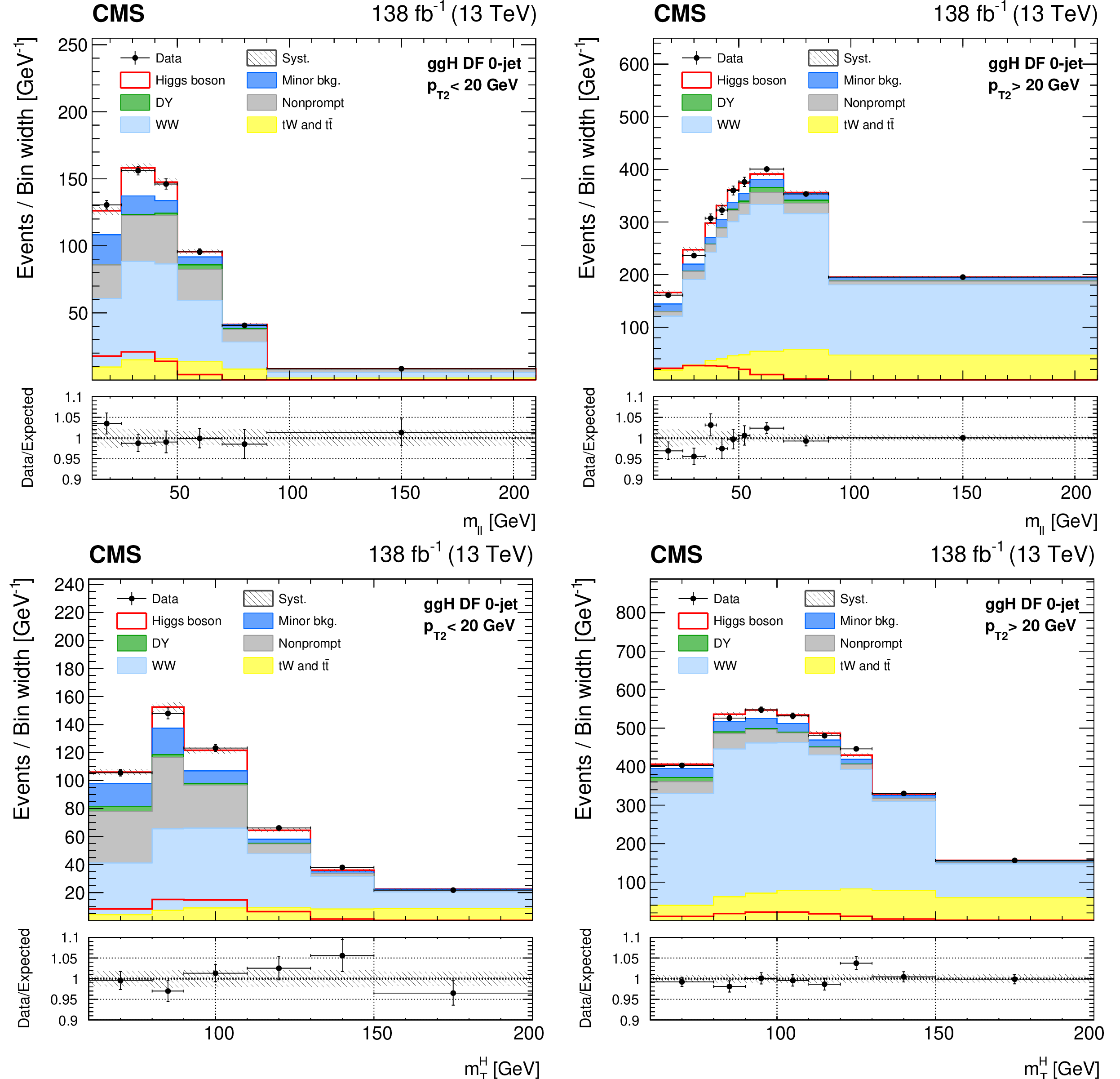
Figure 1:
Observed distributions of the ${m_{\ell \ell}}$ (upper) and ${{m_{\mathrm {T}}} ^{\mathrm{H}}}$ (lower) fit variables in the 0-jet ggH $ {{p_{\mathrm {T}}} {}_2} < $ 20 GeV (left) and $ {{p_{\mathrm {T}}} {}_2} > $ 20 GeV (right) DF categories. The uncertainty band corresponds to the total systematic uncertainty in the templates after the fit to the data. The signal template is shown both stacked on top of the backgrounds, as well as superimposed. The predicted yields are shown with their best fit normalizations from the simultaneous fit. Vertical bars on data points represent the statistical uncertainty in the data. The overflow is included in the last bin. The lower panel in each figure shows the ratio of the number of events observed in data to that of the total SM prediction. |

png pdf |
Figure 1-a:
Observed distributions of the ${m_{\ell \ell}}$ (upper) and ${{m_{\mathrm {T}}} ^{\mathrm{H}}}$ (lower) fit variables in the 0-jet ggH $ {{p_{\mathrm {T}}} {}_2} < $ 20 GeV (left) and $ {{p_{\mathrm {T}}} {}_2} > $ 20 GeV (right) DF categories. The uncertainty band corresponds to the total systematic uncertainty in the templates after the fit to the data. The signal template is shown both stacked on top of the backgrounds, as well as superimposed. The predicted yields are shown with their best fit normalizations from the simultaneous fit. Vertical bars on data points represent the statistical uncertainty in the data. The overflow is included in the last bin. The lower panel in each figure shows the ratio of the number of events observed in data to that of the total SM prediction. |
png pdf |
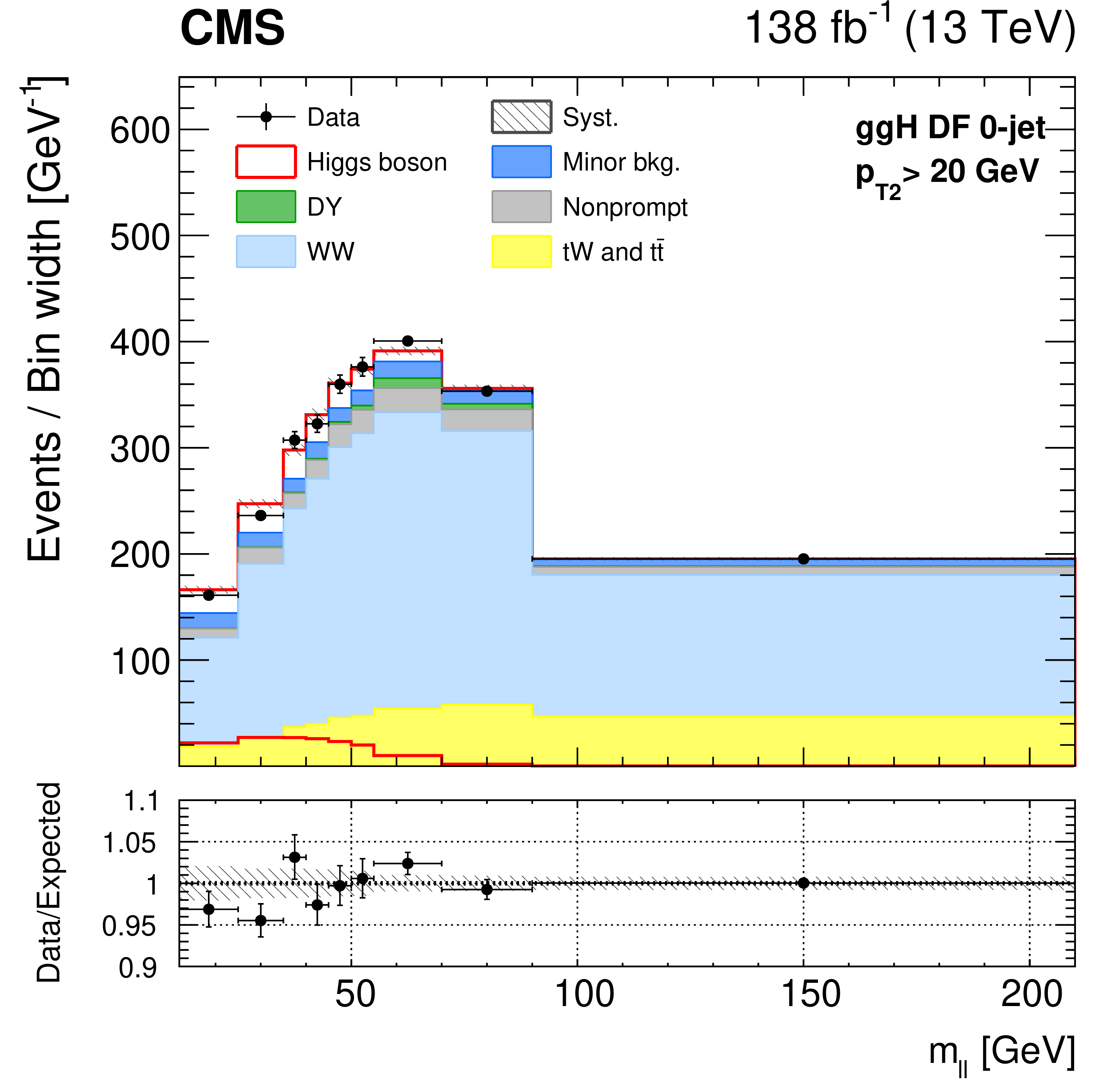
Figure 1-b:
Observed distributions of the ${m_{\ell \ell}}$ (upper) and ${{m_{\mathrm {T}}} ^{\mathrm{H}}}$ (lower) fit variables in the 0-jet ggH $ {{p_{\mathrm {T}}} {}_2} < $ 20 GeV (left) and $ {{p_{\mathrm {T}}} {}_2} > $ 20 GeV (right) DF categories. The uncertainty band corresponds to the total systematic uncertainty in the templates after the fit to the data. The signal template is shown both stacked on top of the backgrounds, as well as superimposed. The predicted yields are shown with their best fit normalizations from the simultaneous fit. Vertical bars on data points represent the statistical uncertainty in the data. The overflow is included in the last bin. The lower panel in each figure shows the ratio of the number of events observed in data to that of the total SM prediction. |
png pdf |
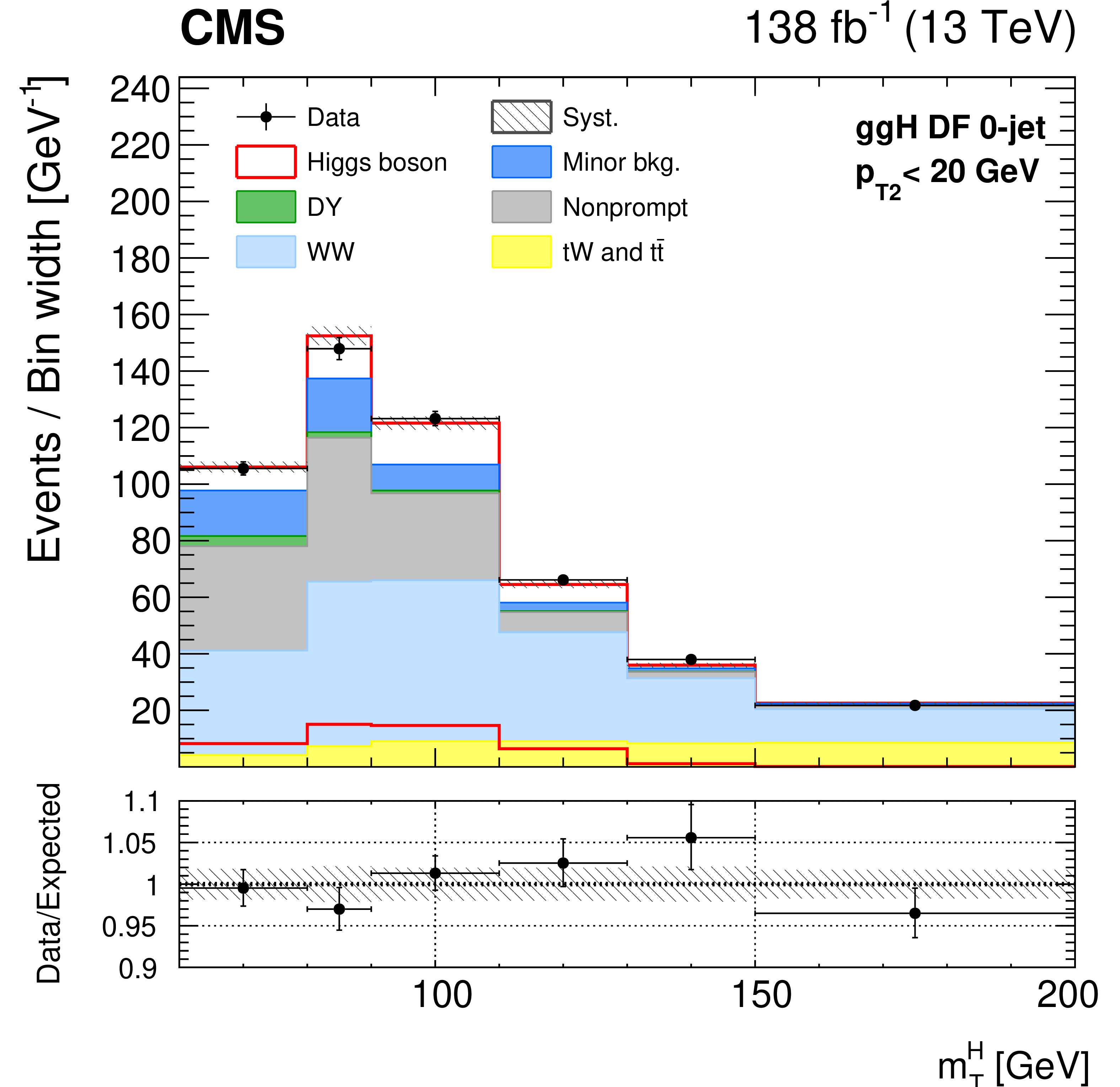
Figure 1-c:
Observed distributions of the ${m_{\ell \ell}}$ (upper) and ${{m_{\mathrm {T}}} ^{\mathrm{H}}}$ (lower) fit variables in the 0-jet ggH $ {{p_{\mathrm {T}}} {}_2} < $ 20 GeV (left) and $ {{p_{\mathrm {T}}} {}_2} > $ 20 GeV (right) DF categories. The uncertainty band corresponds to the total systematic uncertainty in the templates after the fit to the data. The signal template is shown both stacked on top of the backgrounds, as well as superimposed. The predicted yields are shown with their best fit normalizations from the simultaneous fit. Vertical bars on data points represent the statistical uncertainty in the data. The overflow is included in the last bin. The lower panel in each figure shows the ratio of the number of events observed in data to that of the total SM prediction. |
png pdf |
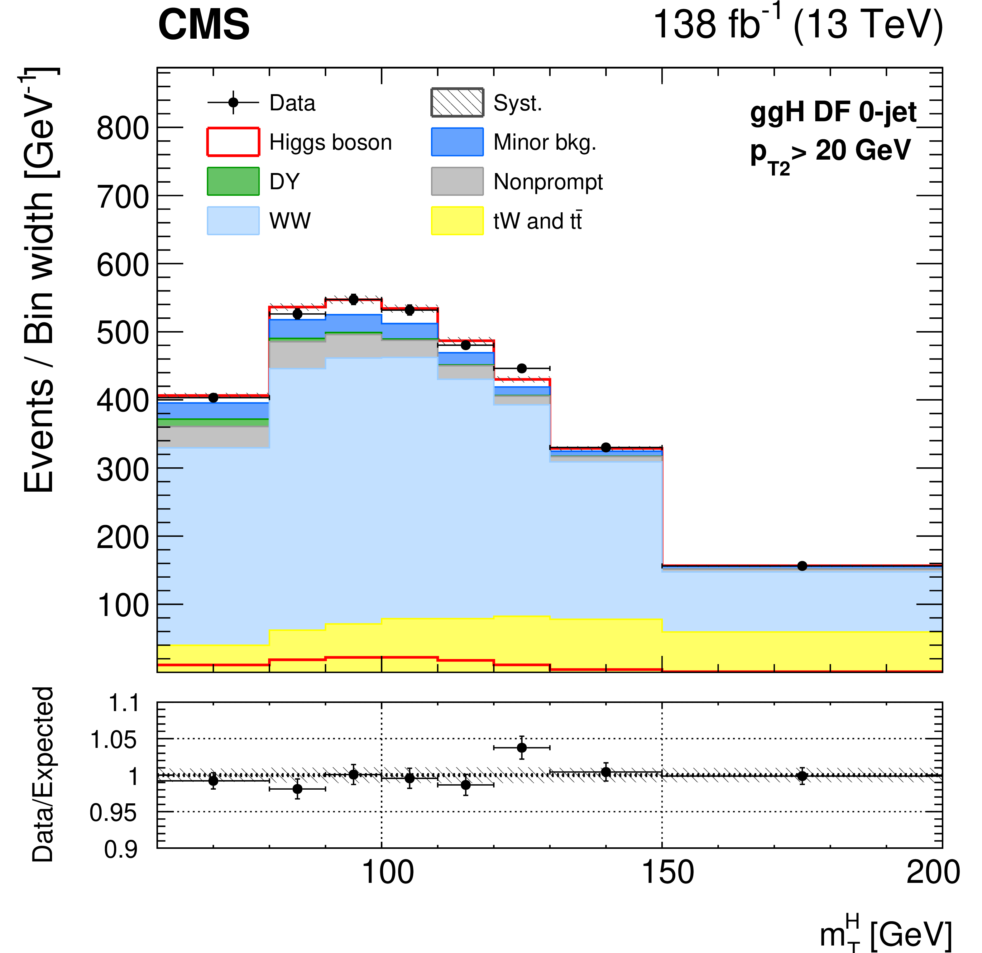
Figure 1-d:
Observed distributions of the ${m_{\ell \ell}}$ (upper) and ${{m_{\mathrm {T}}} ^{\mathrm{H}}}$ (lower) fit variables in the 0-jet ggH $ {{p_{\mathrm {T}}} {}_2} < $ 20 GeV (left) and $ {{p_{\mathrm {T}}} {}_2} > $ 20 GeV (right) DF categories. The uncertainty band corresponds to the total systematic uncertainty in the templates after the fit to the data. The signal template is shown both stacked on top of the backgrounds, as well as superimposed. The predicted yields are shown with their best fit normalizations from the simultaneous fit. Vertical bars on data points represent the statistical uncertainty in the data. The overflow is included in the last bin. The lower panel in each figure shows the ratio of the number of events observed in data to that of the total SM prediction. |
png pdf |
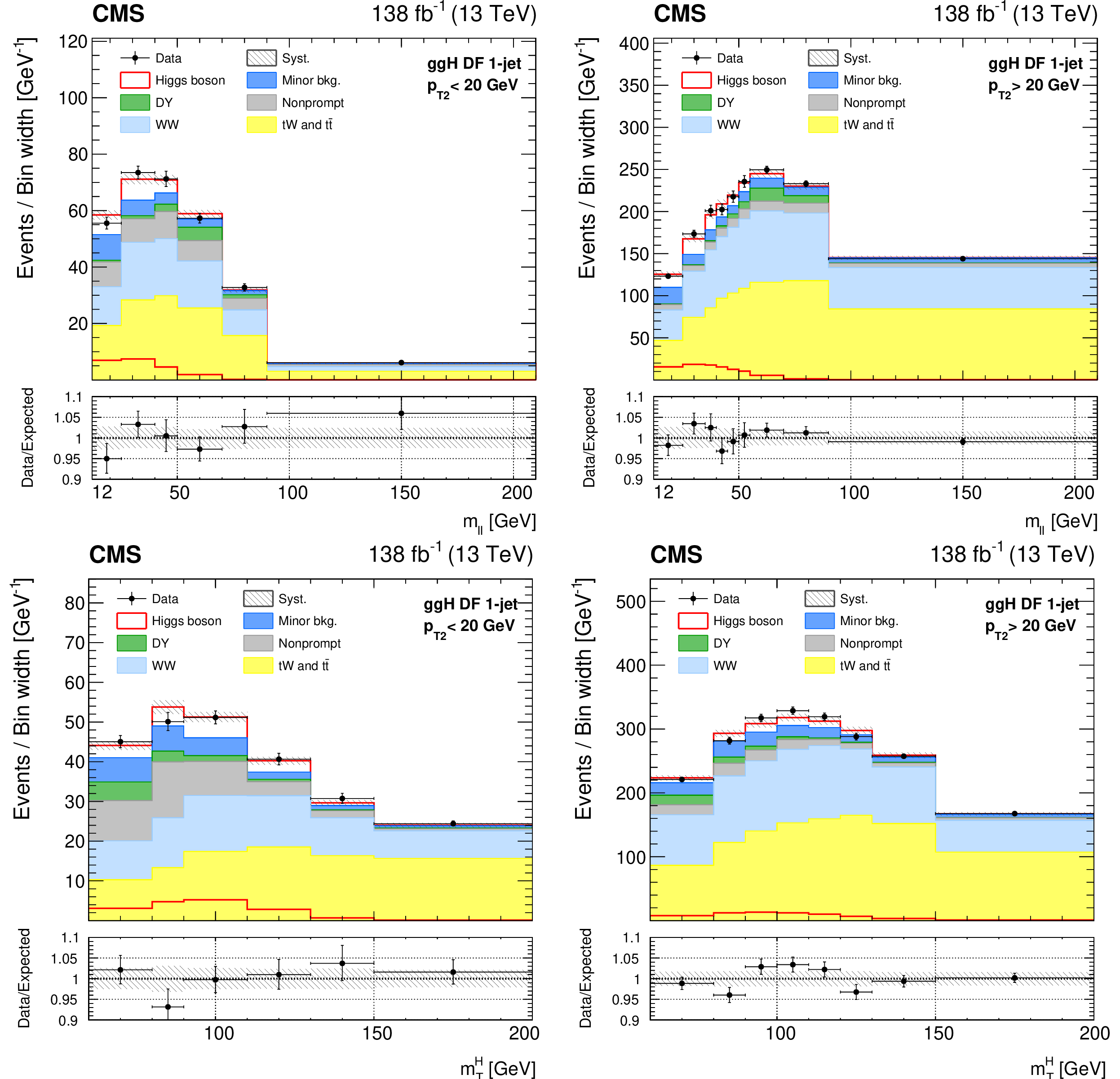
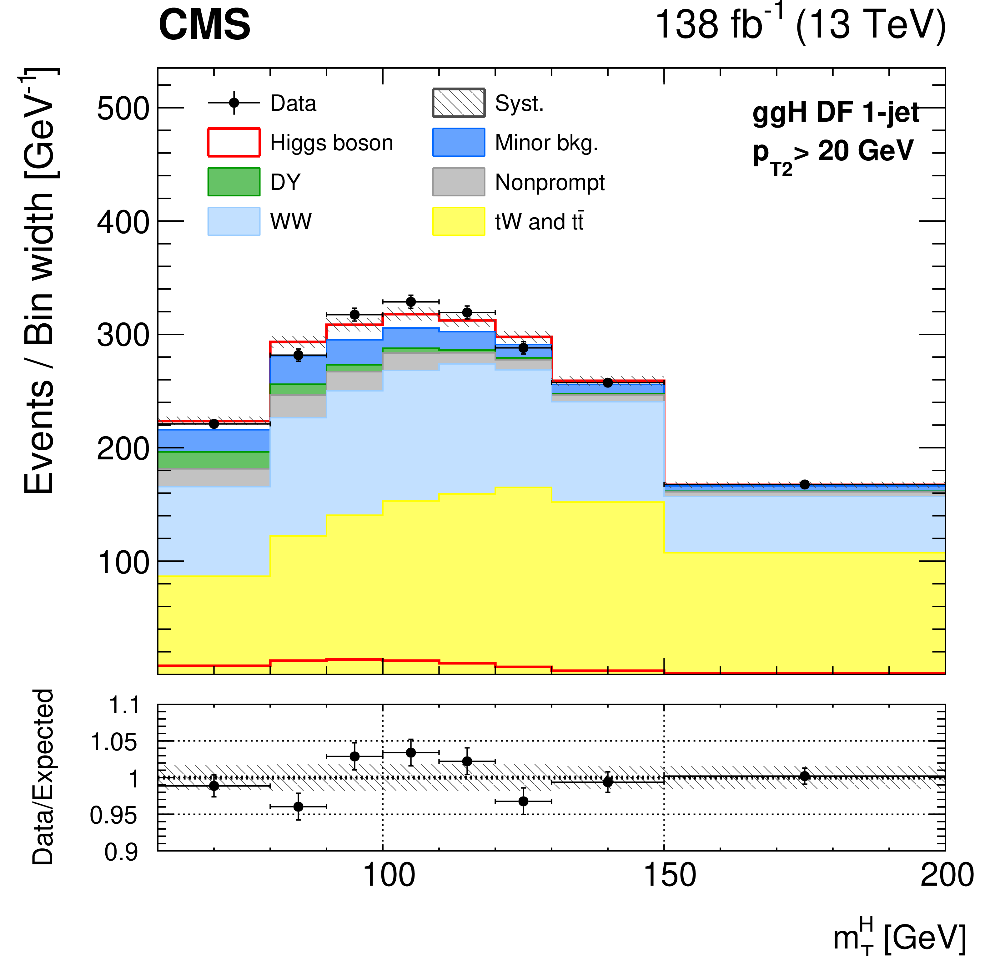
Figure 2:
Observed distributions of the ${m_{\ell \ell}}$ (upper) and ${{m_{\mathrm {T}}} ^{\mathrm{H}}}$ (lower) fit variables in the 1-jet ggH $ {{p_{\mathrm {T}}} {}_2} < $ 20 GeV (left) and $ {{p_{\mathrm {T}}} {}_2} > $ 20 GeV (right) DF categories. A detailed description is given in the Fig. 1 caption. |
png pdf |
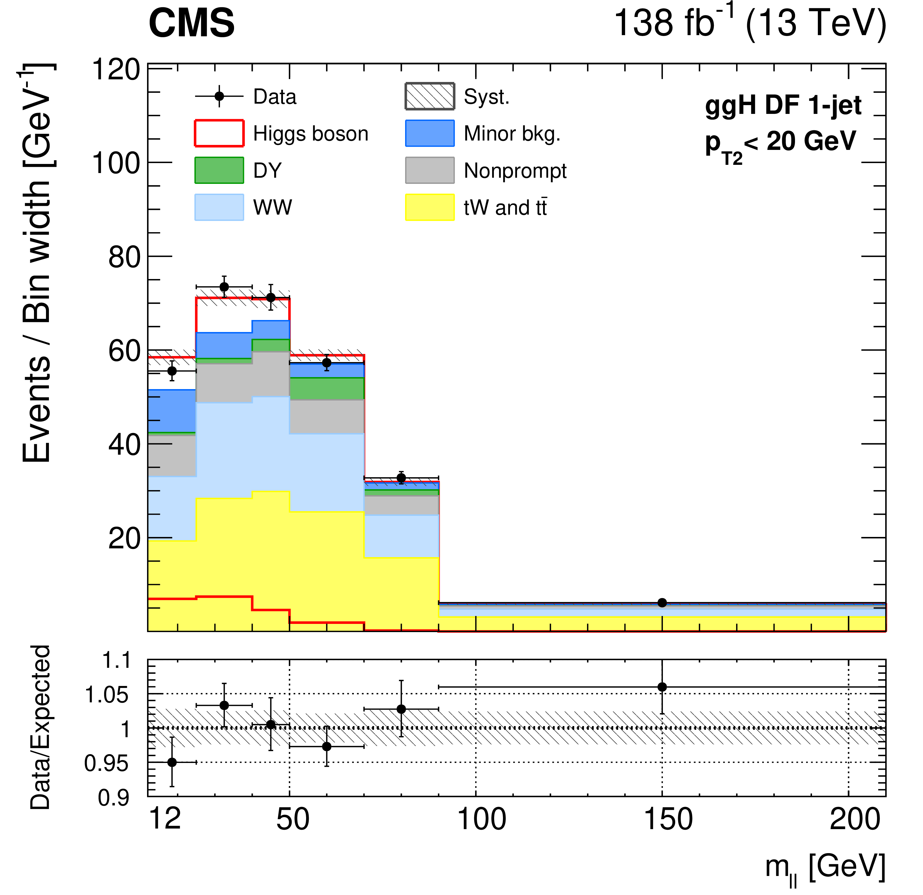
Figure 2-a:
Observed distributions of the ${m_{\ell \ell}}$ (upper) and ${{m_{\mathrm {T}}} ^{\mathrm{H}}}$ (lower) fit variables in the 1-jet ggH $ {{p_{\mathrm {T}}} {}_2} < $ 20 GeV (left) and $ {{p_{\mathrm {T}}} {}_2} > $ 20 GeV (right) DF categories. A detailed description is given in the Fig. 1 caption. |
png pdf |
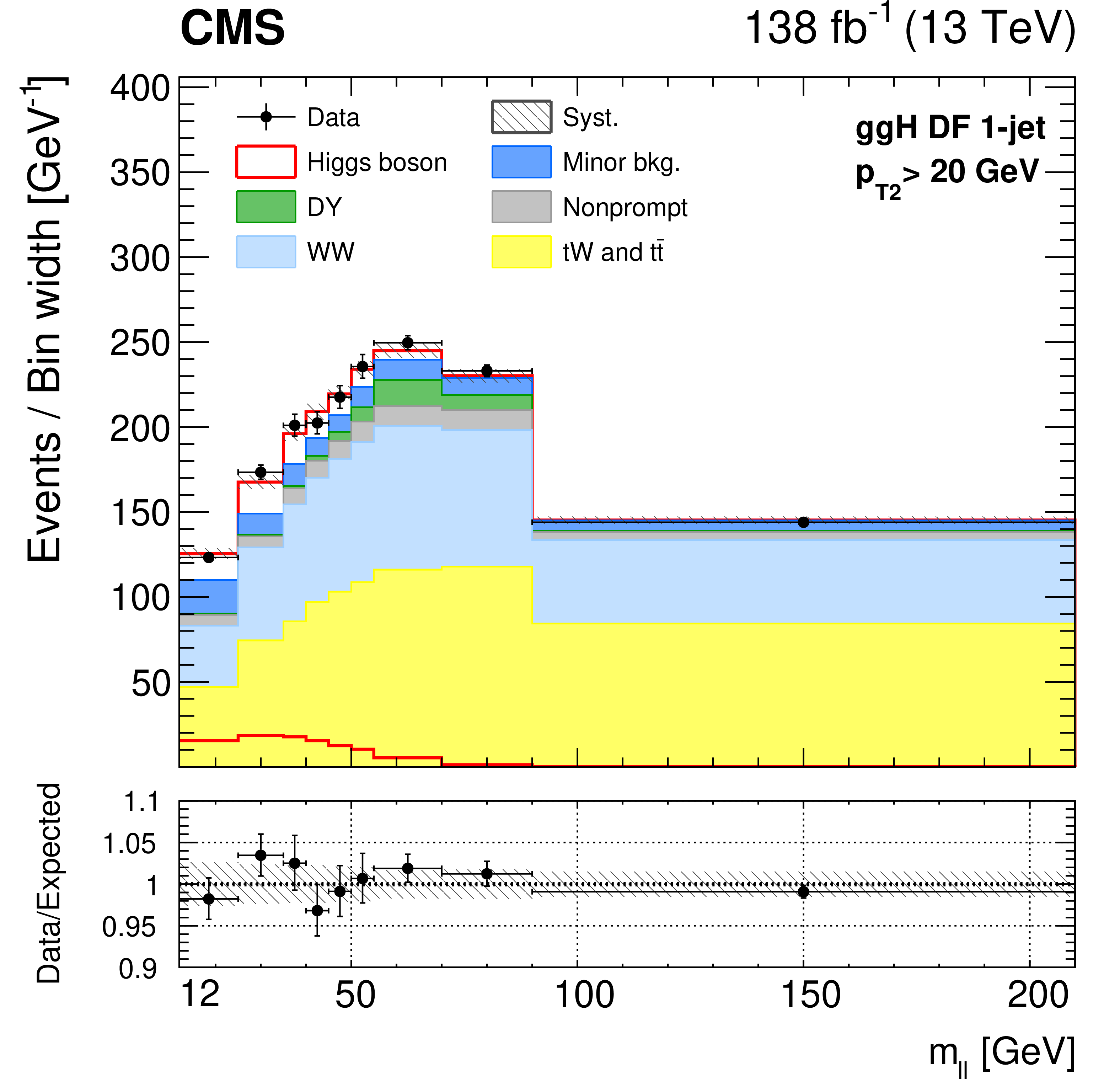
Figure 2-b:
Observed distributions of the ${m_{\ell \ell}}$ (upper) and ${{m_{\mathrm {T}}} ^{\mathrm{H}}}$ (lower) fit variables in the 1-jet ggH $ {{p_{\mathrm {T}}} {}_2} < $ 20 GeV (left) and $ {{p_{\mathrm {T}}} {}_2} > $ 20 GeV (right) DF categories. A detailed description is given in the Fig. 1 caption. |
png pdf |
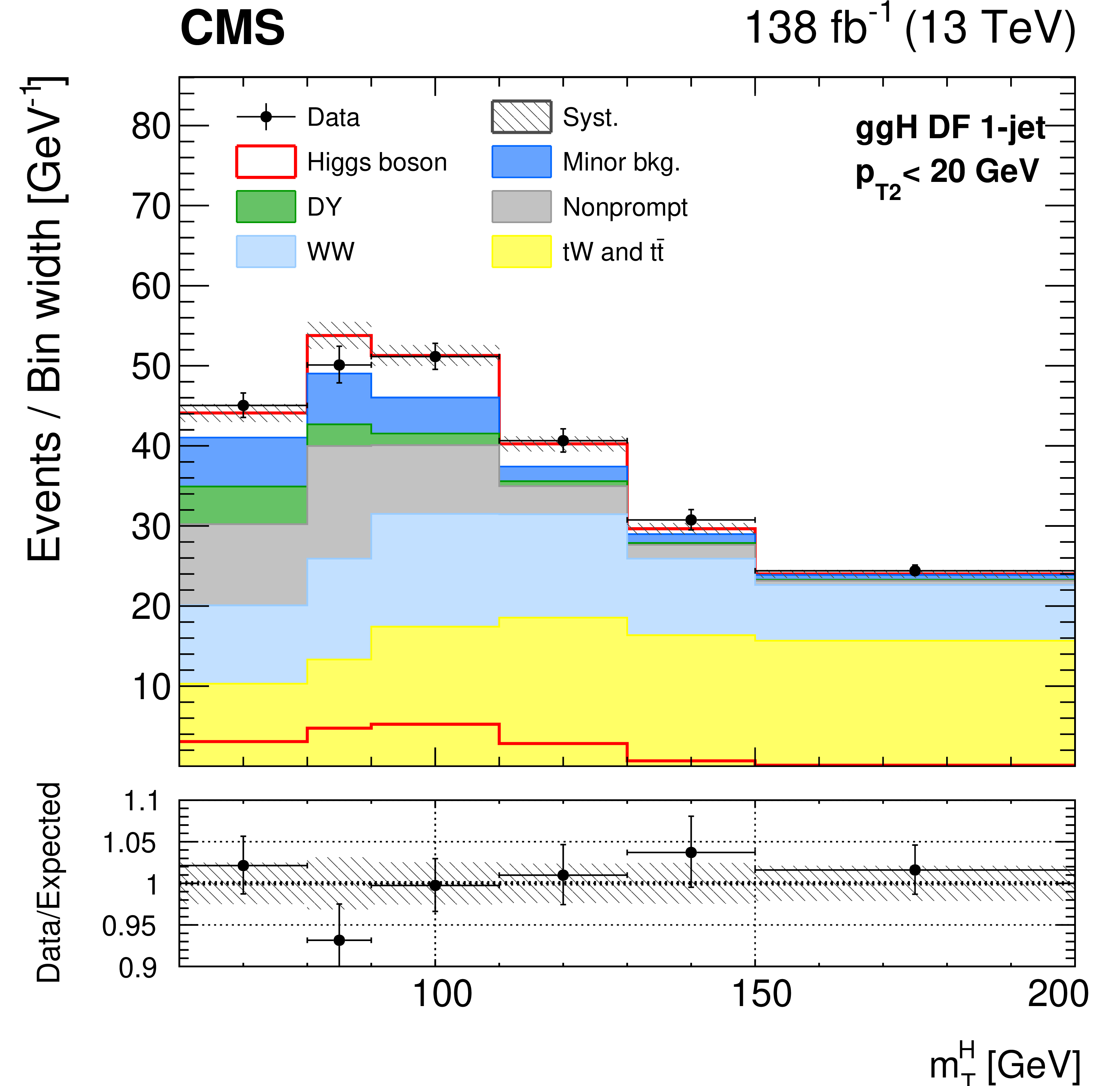
Figure 2-c:
Observed distributions of the ${m_{\ell \ell}}$ (upper) and ${{m_{\mathrm {T}}} ^{\mathrm{H}}}$ (lower) fit variables in the 1-jet ggH $ {{p_{\mathrm {T}}} {}_2} < $ 20 GeV (left) and $ {{p_{\mathrm {T}}} {}_2} > $ 20 GeV (right) DF categories. A detailed description is given in the Fig. 1 caption. |
png pdf |
Figure 2-d:
Observed distributions of the ${m_{\ell \ell}}$ (upper) and ${{m_{\mathrm {T}}} ^{\mathrm{H}}}$ (lower) fit variables in the 1-jet ggH $ {{p_{\mathrm {T}}} {}_2} < $ 20 GeV (left) and $ {{p_{\mathrm {T}}} {}_2} > $ 20 GeV (right) DF categories. A detailed description is given in the Fig. 1 caption. |

png pdf |
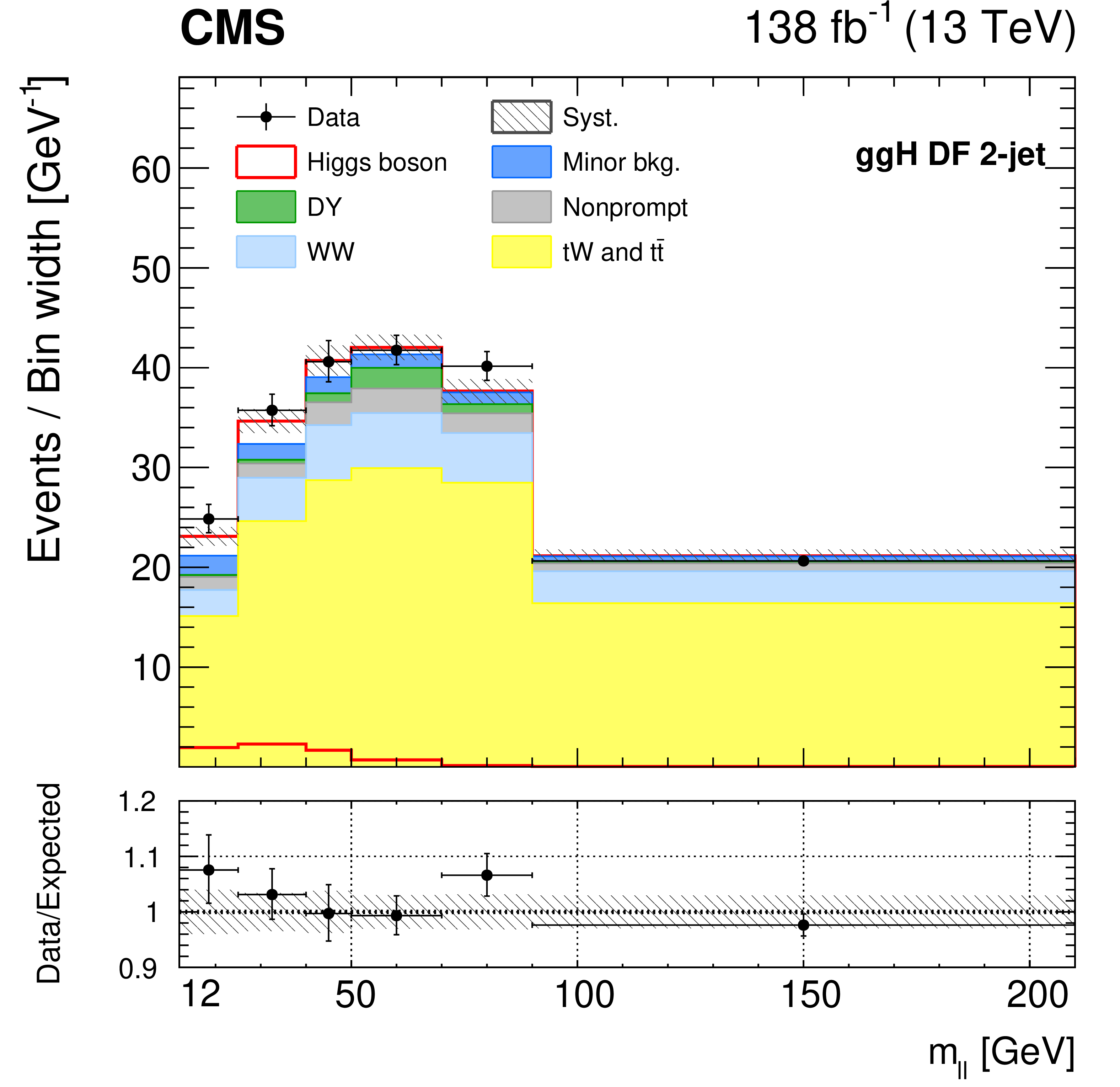
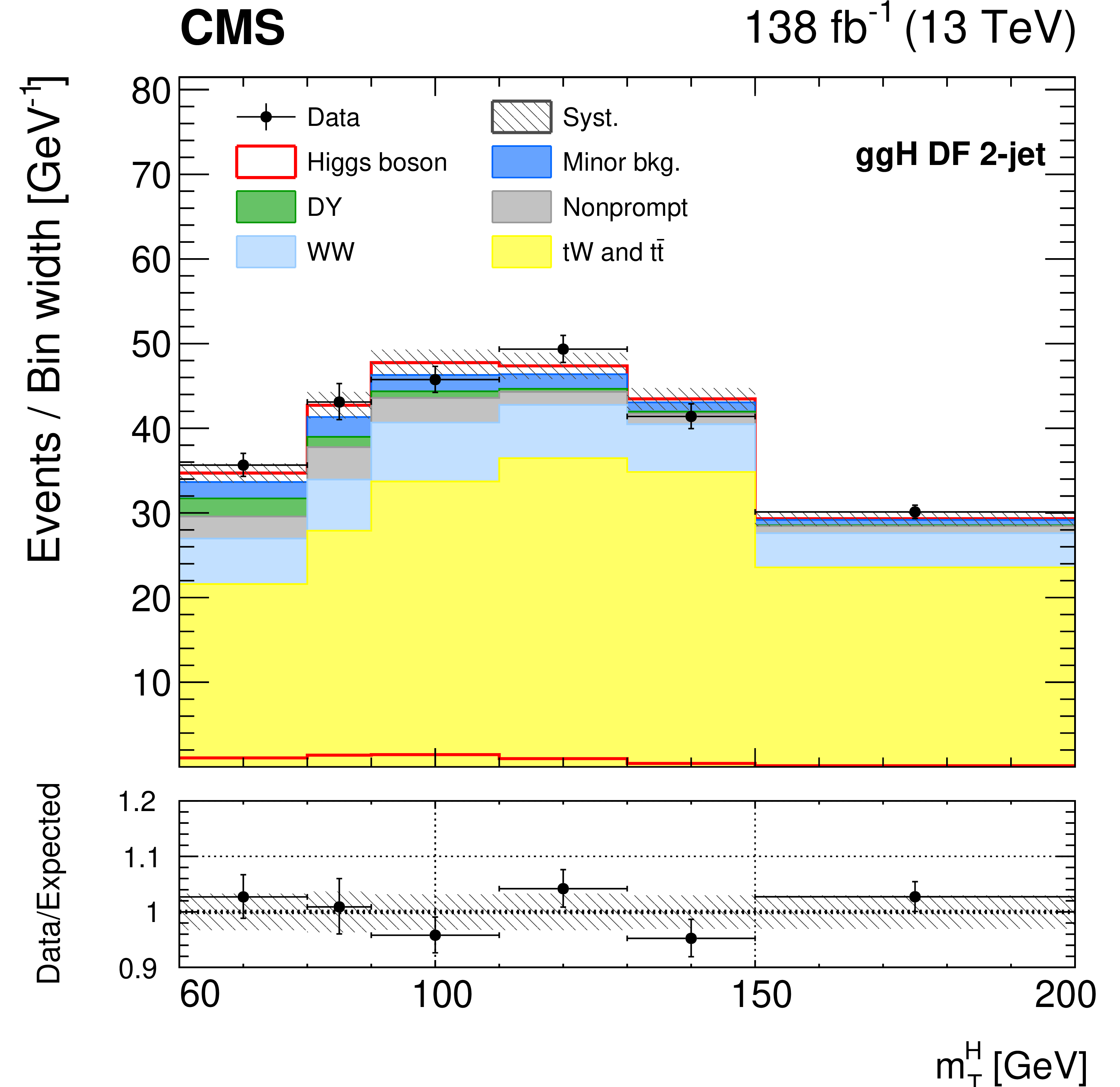
Figure 3:
Observed distributions of the ${m_{\ell \ell}}$ (left) and ${{m_{\mathrm {T}}} ^{\mathrm{H}}}$ (right) fit variables in the 2-jet ggH DF category. A detailed description is given in the Fig. 1 caption. |
png pdf |
Figure 3-a:
Observed distributions of the ${m_{\ell \ell}}$ (left) and ${{m_{\mathrm {T}}} ^{\mathrm{H}}}$ (right) fit variables in the 2-jet ggH DF category. A detailed description is given in the Fig. 1 caption. |
png pdf |
Figure 3-b:
Observed distributions of the ${m_{\ell \ell}}$ (left) and ${{m_{\mathrm {T}}} ^{\mathrm{H}}}$ (right) fit variables in the 2-jet ggH DF category. A detailed description is given in the Fig. 1 caption. |
png pdf |
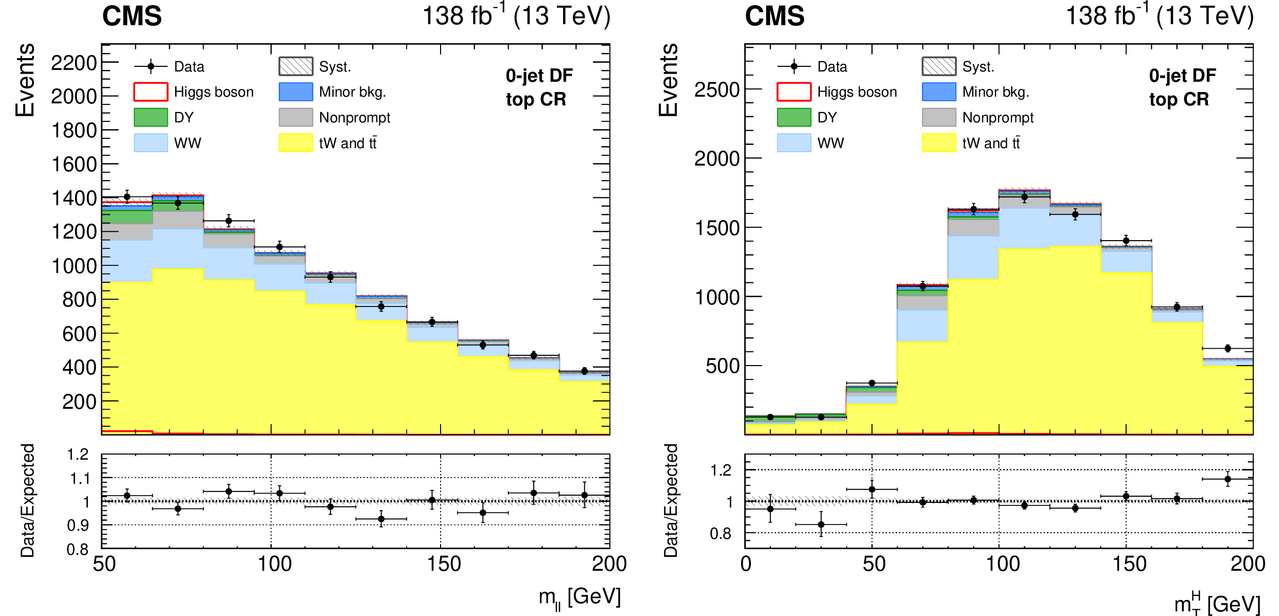
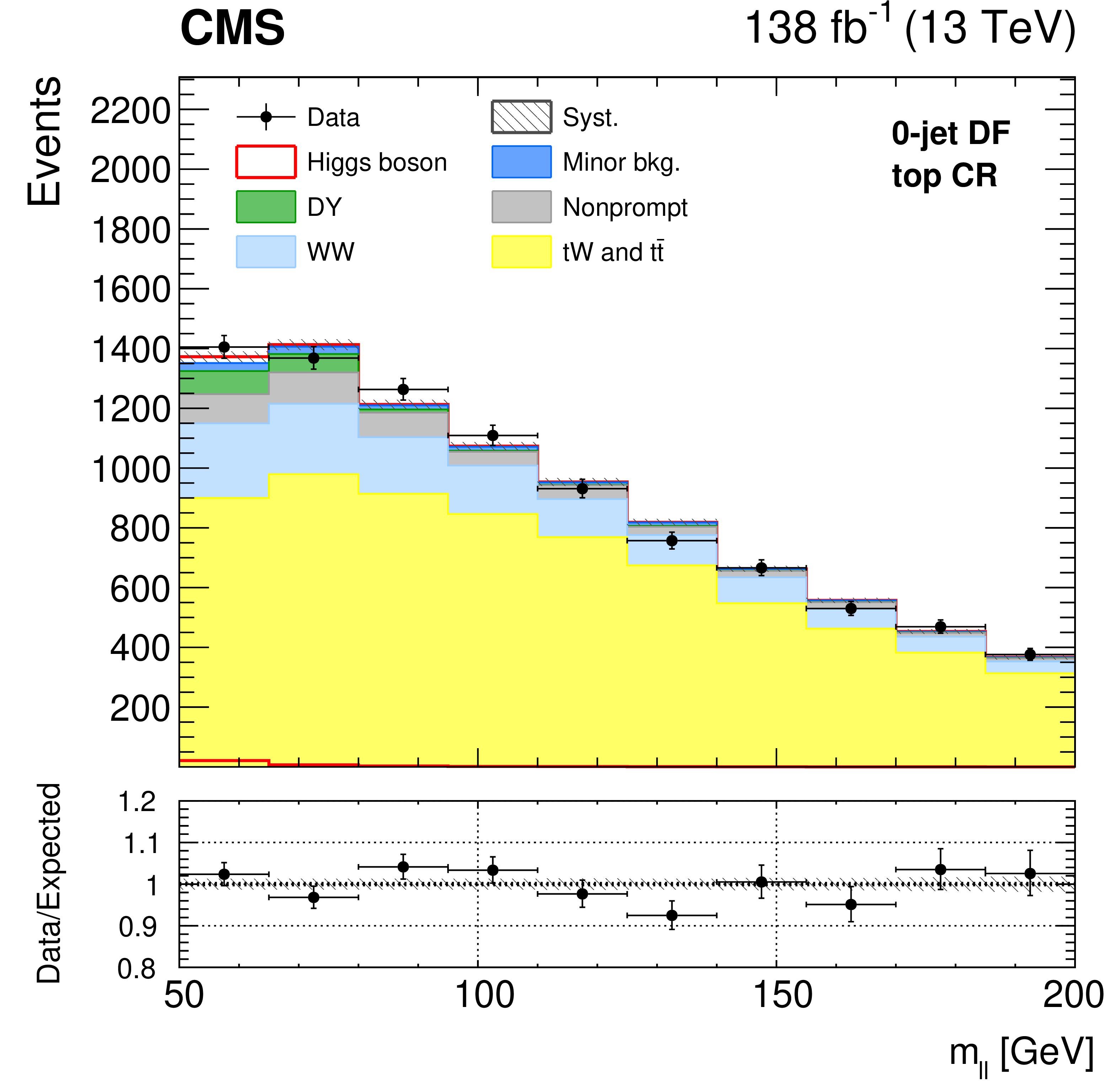
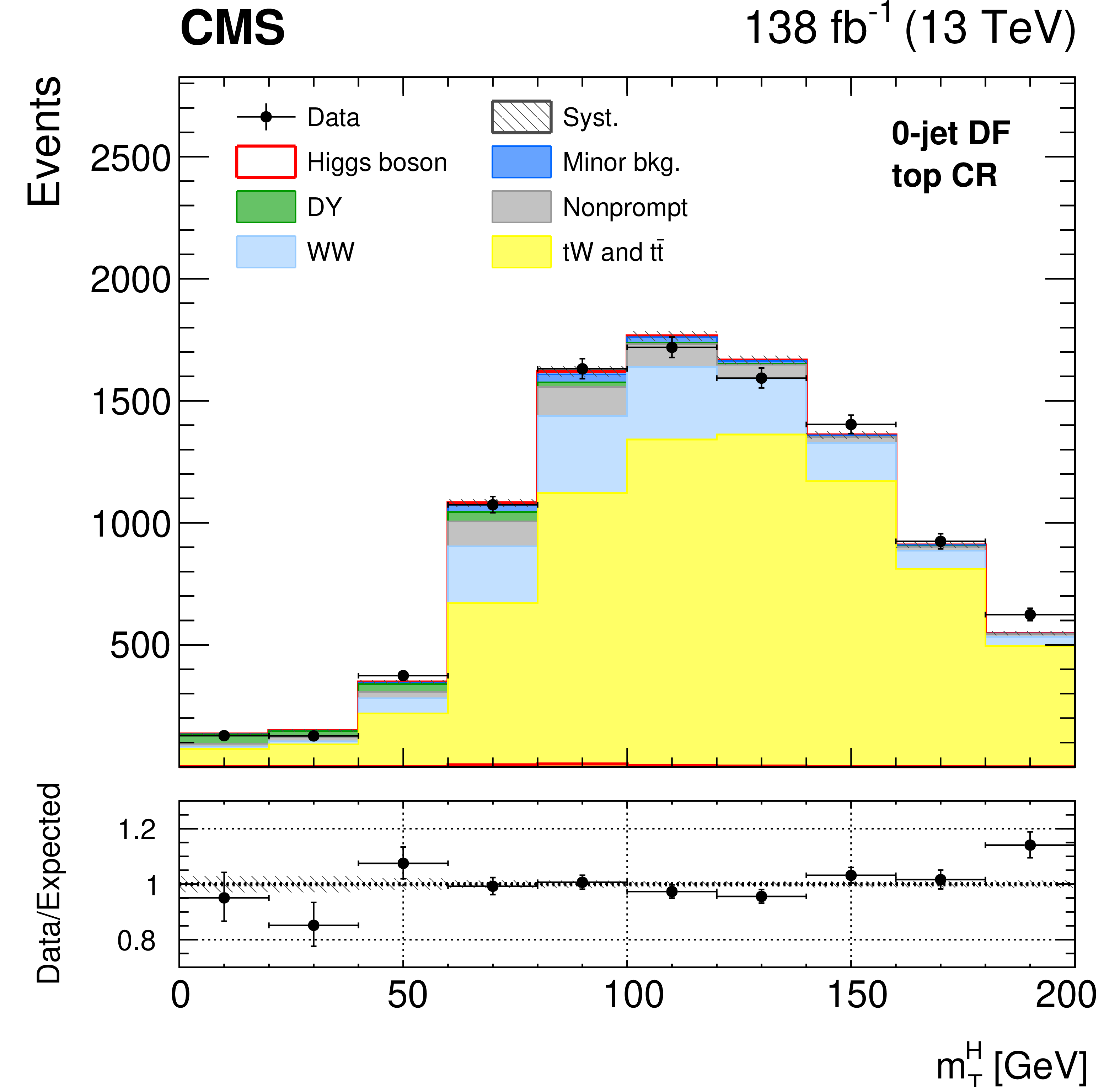
Figure 4:
Observed distributions of the ${m_{\ell \ell}}$ (left) and ${{m_{\mathrm {T}}} ^{\mathrm{H}}}$ (right) variables in the 0-jet DF top quark control region. A detailed description is given in the Fig. 1 caption. |
png pdf |
Figure 4-a:
Observed distributions of the ${m_{\ell \ell}}$ (left) and ${{m_{\mathrm {T}}} ^{\mathrm{H}}}$ (right) variables in the 0-jet DF top quark control region. A detailed description is given in the Fig. 1 caption. |
png pdf |
Figure 4-b:
Observed distributions of the ${m_{\ell \ell}}$ (left) and ${{m_{\mathrm {T}}} ^{\mathrm{H}}}$ (right) variables in the 0-jet DF top quark control region. A detailed description is given in the Fig. 1 caption. |
png pdf |
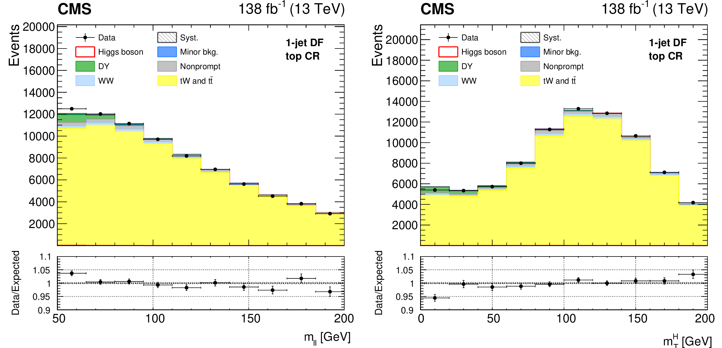
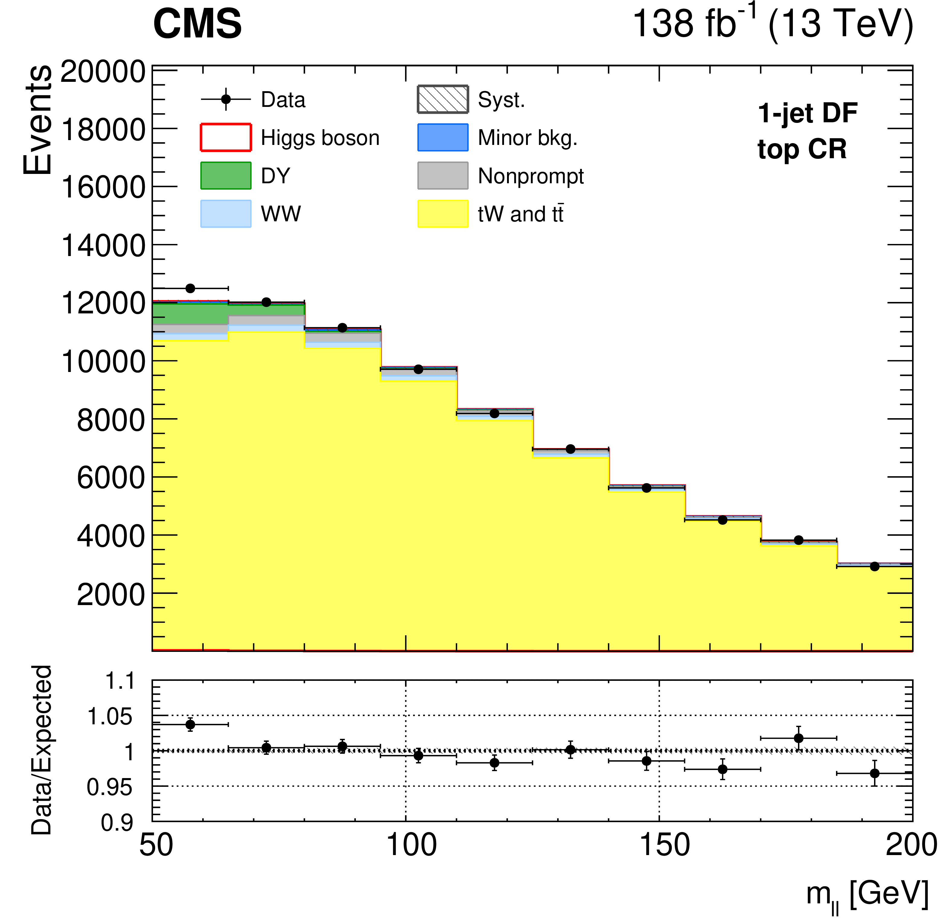
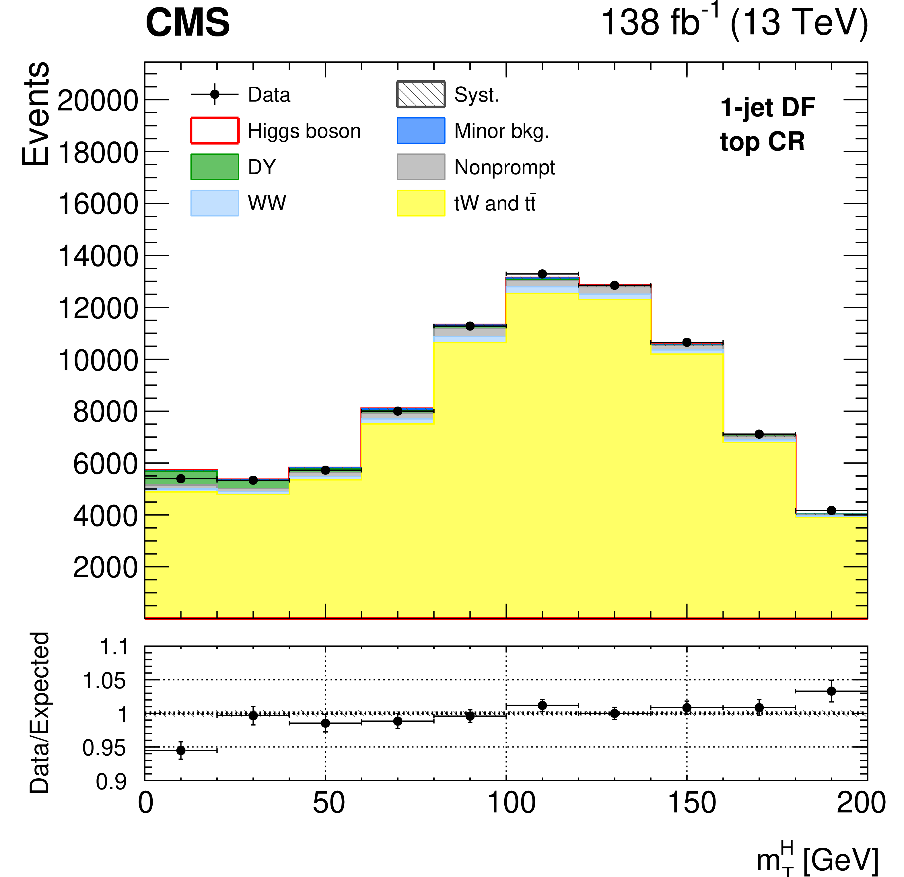
Figure 5:
Observed distributions of the ${m_{\ell \ell}}$ (left) and ${{m_{\mathrm {T}}} ^{\mathrm{H}}}$ (right) variables in the 1-jet DF top quark control region. A detailed description is given in the Fig. 1 caption. |
png pdf |
Figure 5-a:
Observed distributions of the ${m_{\ell \ell}}$ (left) and ${{m_{\mathrm {T}}} ^{\mathrm{H}}}$ (right) variables in the 1-jet DF top quark control region. A detailed description is given in the Fig. 1 caption. |
png pdf |
Figure 5-b:
Observed distributions of the ${m_{\ell \ell}}$ (left) and ${{m_{\mathrm {T}}} ^{\mathrm{H}}}$ (right) variables in the 1-jet DF top quark control region. A detailed description is given in the Fig. 1 caption. |
png pdf |
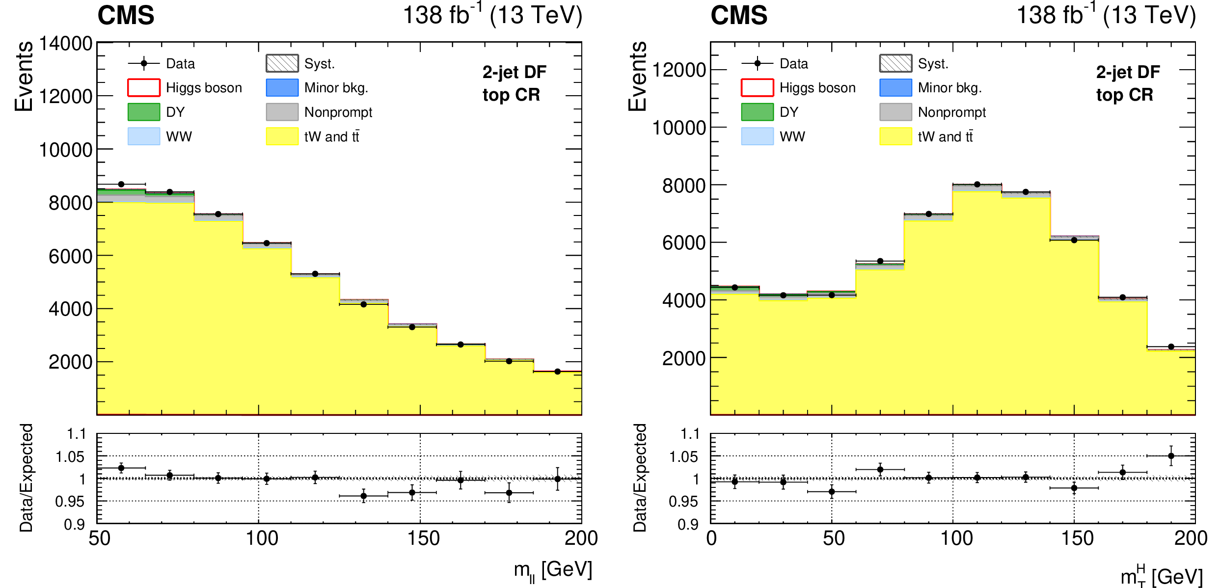
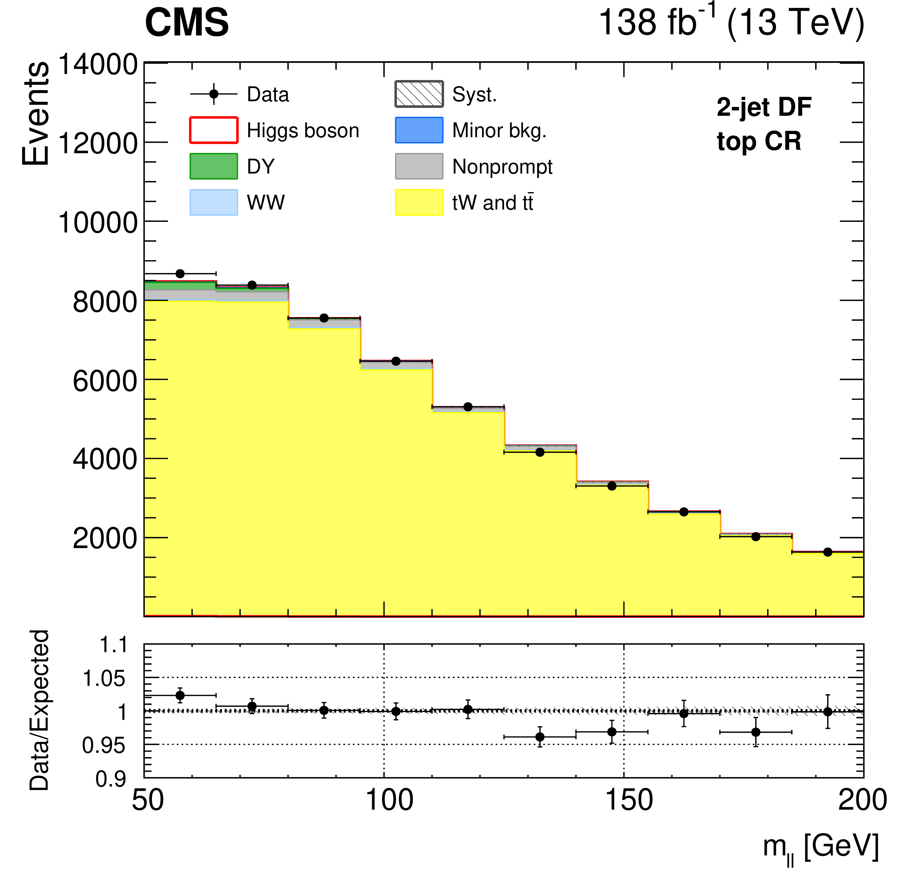
Figure 6:
Observed distributions of the ${m_{\ell \ell}}$ (left) and ${{m_{\mathrm {T}}} ^{\mathrm{H}}}$ (right) variables in the 2-jet DF top quark control region. A detailed description is given in the Fig. 1 caption. |
png pdf |
Figure 6-a:
Observed distributions of the ${m_{\ell \ell}}$ (left) and ${{m_{\mathrm {T}}} ^{\mathrm{H}}}$ (right) variables in the 2-jet DF top quark control region. A detailed description is given in the Fig. 1 caption. |

png pdf |
Figure 6-b:
Observed distributions of the ${m_{\ell \ell}}$ (left) and ${{m_{\mathrm {T}}} ^{\mathrm{H}}}$ (right) variables in the 2-jet DF top quark control region. A detailed description is given in the Fig. 1 caption. |
png pdf |
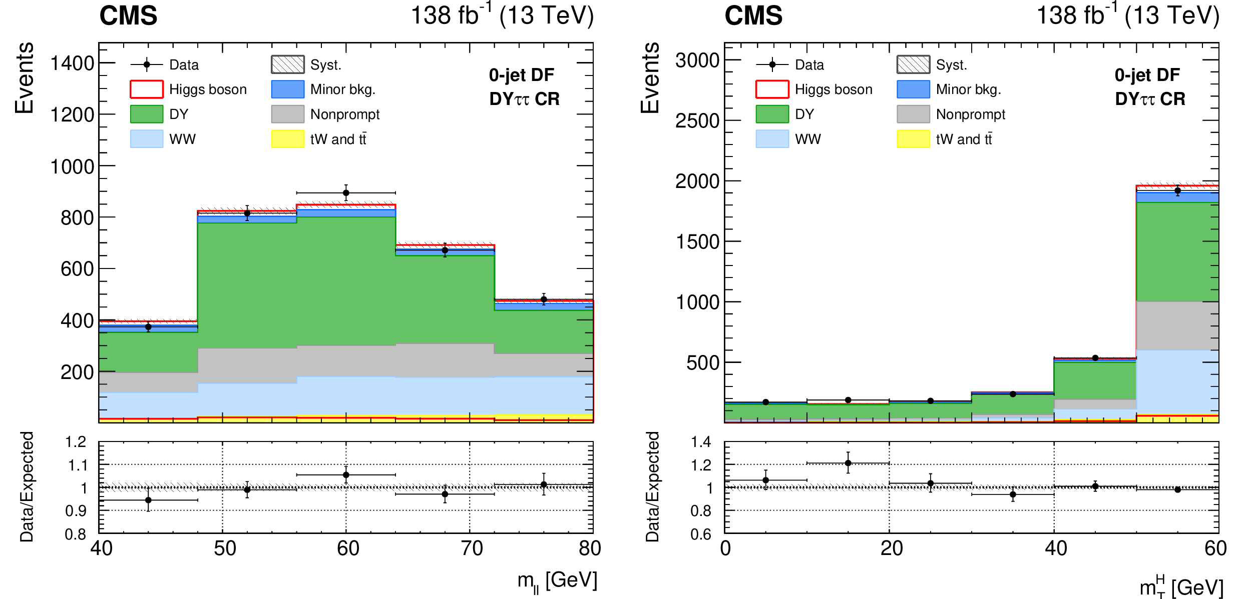
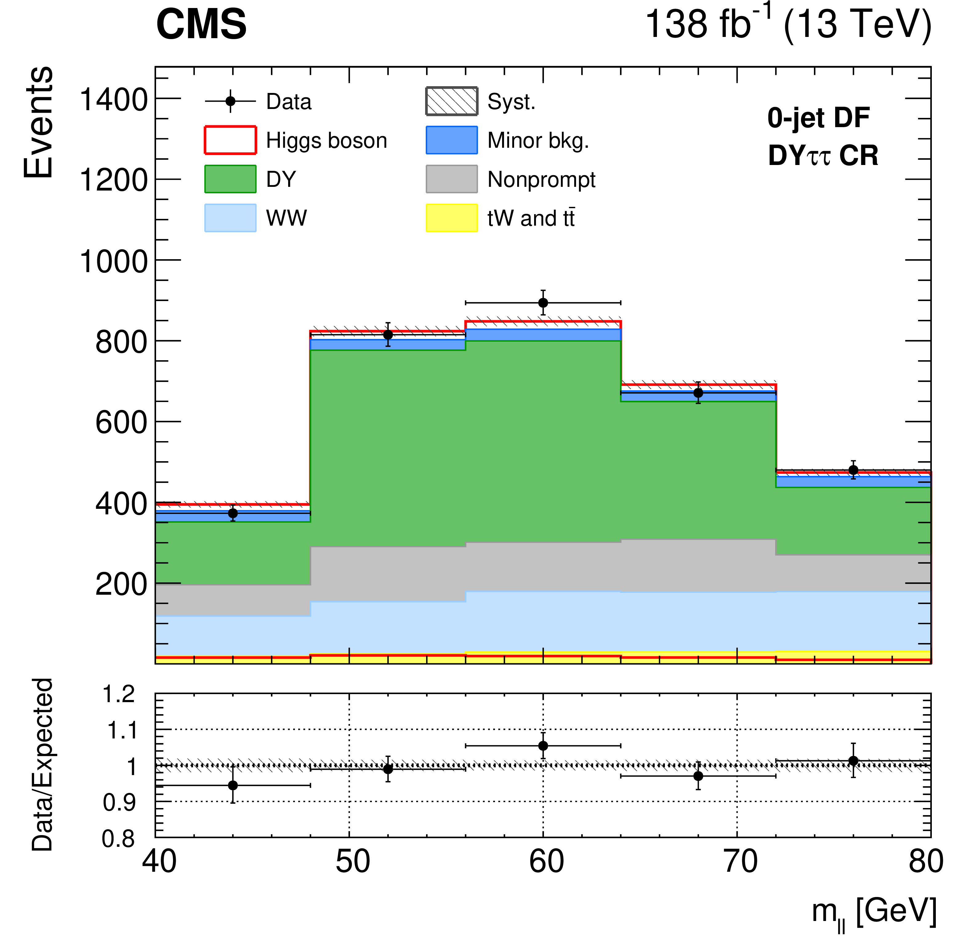
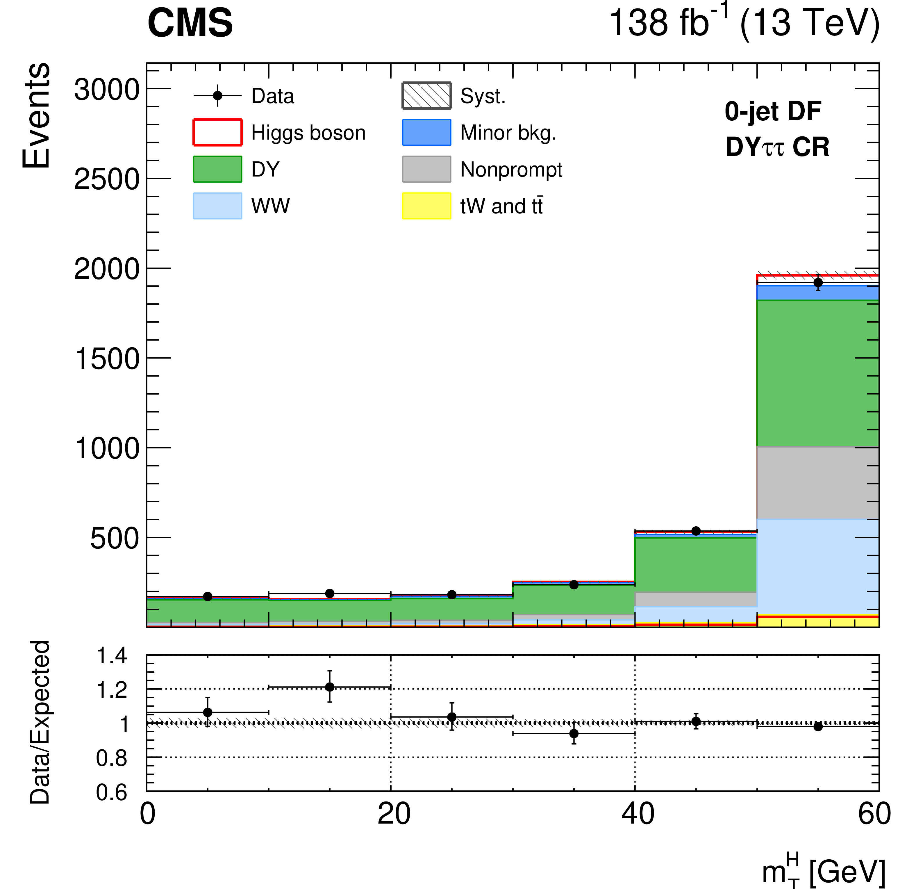
Figure 7:
Observed distributions of the ${m_{\ell \ell}}$ (left) and ${{m_{\mathrm {T}}} ^{\mathrm{H}}}$ (right) variables in the 0-jet DF ${\tau \tau}$ control region. A detailed description is given in the Fig. 1 caption. |
png pdf |
Figure 7-a:
Observed distributions of the ${m_{\ell \ell}}$ (left) and ${{m_{\mathrm {T}}} ^{\mathrm{H}}}$ (right) variables in the 0-jet DF ${\tau \tau}$ control region. A detailed description is given in the Fig. 1 caption. |
png pdf |
Figure 7-b:
Observed distributions of the ${m_{\ell \ell}}$ (left) and ${{m_{\mathrm {T}}} ^{\mathrm{H}}}$ (right) variables in the 0-jet DF ${\tau \tau}$ control region. A detailed description is given in the Fig. 1 caption. |
png pdf |
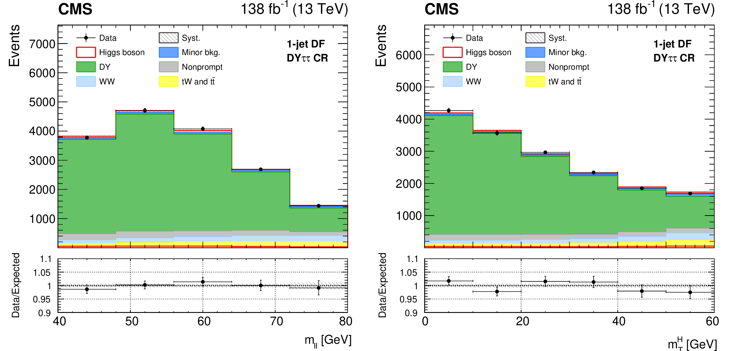
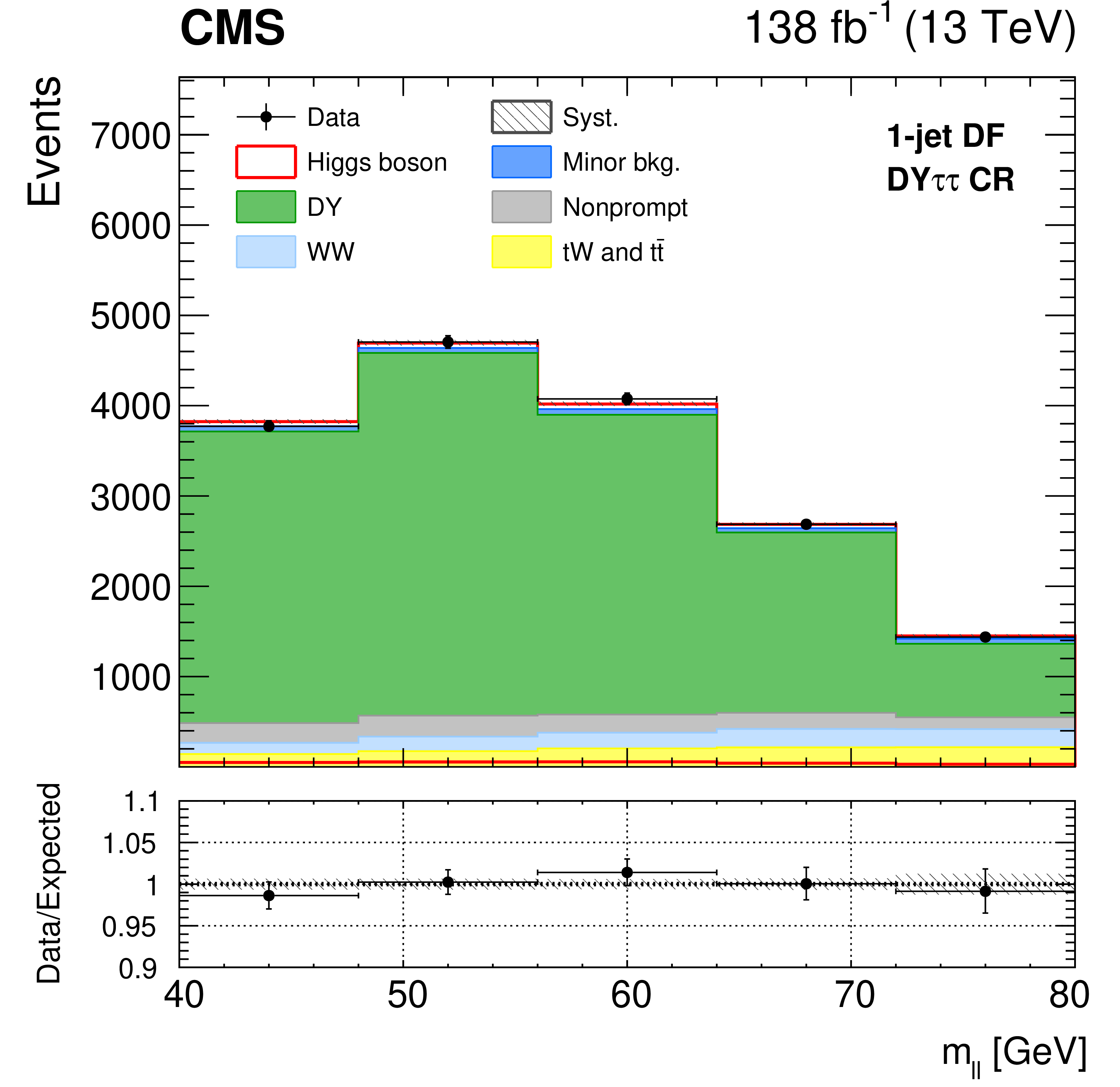
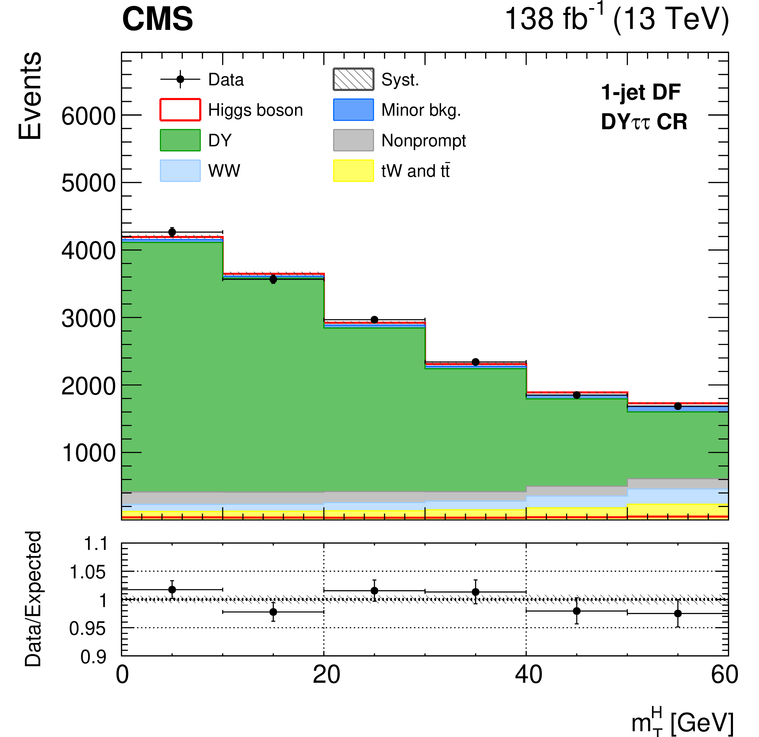
Figure 8:
Observed distributions of the ${m_{\ell \ell}}$ (left) and ${{m_{\mathrm {T}}} ^{\mathrm{H}}}$ (right) variables in the 1-jet DF ${\tau \tau}$ control region. A detailed description is given in the Fig. 1 caption. |
png pdf |
Figure 8-a:
Observed distributions of the ${m_{\ell \ell}}$ (left) and ${{m_{\mathrm {T}}} ^{\mathrm{H}}}$ (right) variables in the 1-jet DF ${\tau \tau}$ control region. A detailed description is given in the Fig. 1 caption. |
png pdf |
Figure 8-b:
Observed distributions of the ${m_{\ell \ell}}$ (left) and ${{m_{\mathrm {T}}} ^{\mathrm{H}}}$ (right) variables in the 1-jet DF ${\tau \tau}$ control region. A detailed description is given in the Fig. 1 caption. |

png pdf |
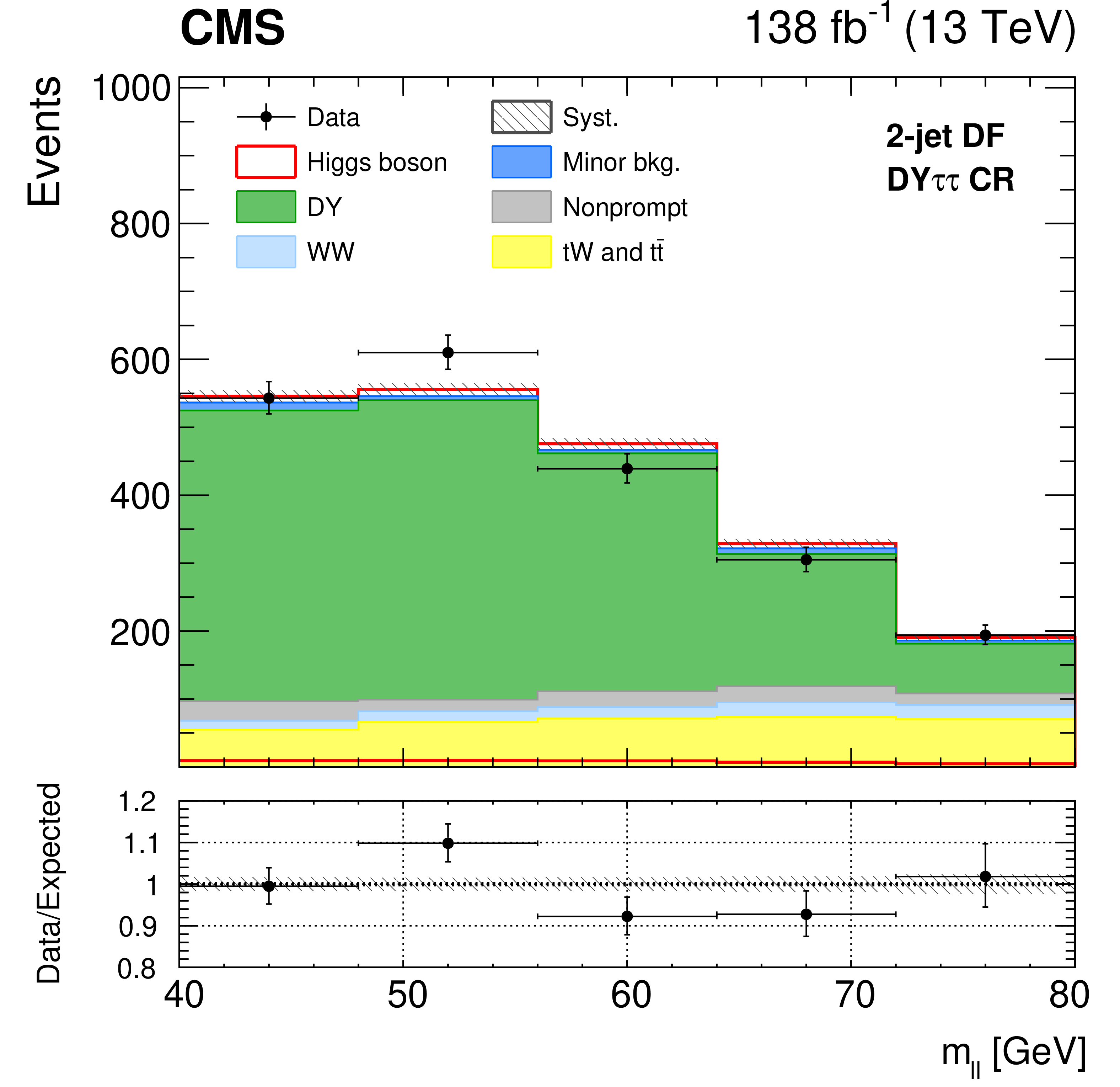
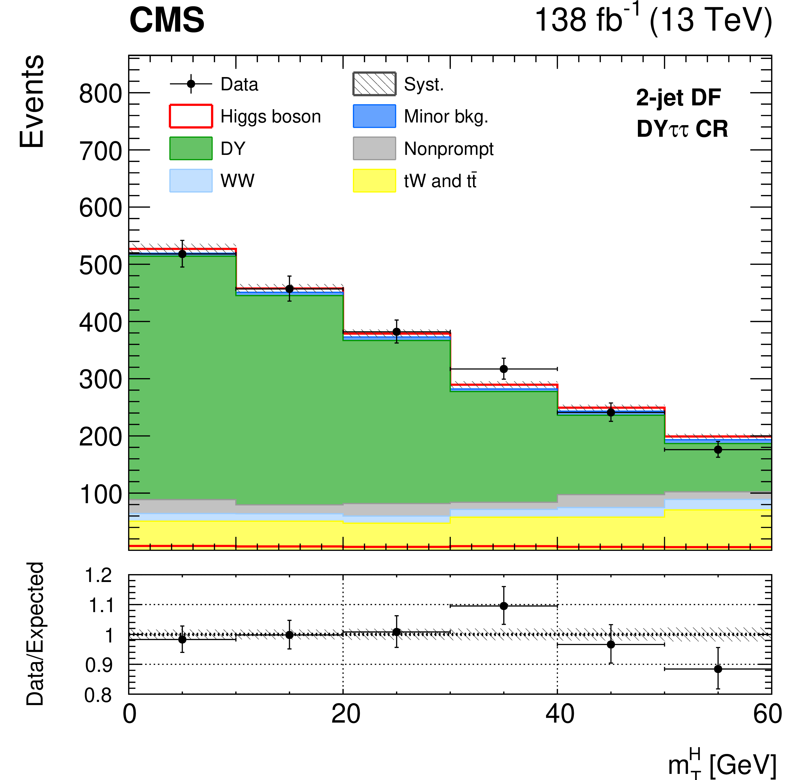
Figure 9:
Observed distributions of the ${m_{\ell \ell}}$ (left) and ${{m_{\mathrm {T}}} ^{\mathrm{H}}}$ (right) variables in the 2-jet DF ${\tau \tau}$ control region. A detailed description is given in the Fig. 1 caption. |
png pdf |
Figure 9-a:
Observed distributions of the ${m_{\ell \ell}}$ (left) and ${{m_{\mathrm {T}}} ^{\mathrm{H}}}$ (right) variables in the 2-jet DF ${\tau \tau}$ control region. A detailed description is given in the Fig. 1 caption. |
png pdf |
Figure 9-b:
Observed distributions of the ${m_{\ell \ell}}$ (left) and ${{m_{\mathrm {T}}} ^{\mathrm{H}}}$ (right) variables in the 2-jet DF ${\tau \tau}$ control region. A detailed description is given in the Fig. 1 caption. |
png pdf |
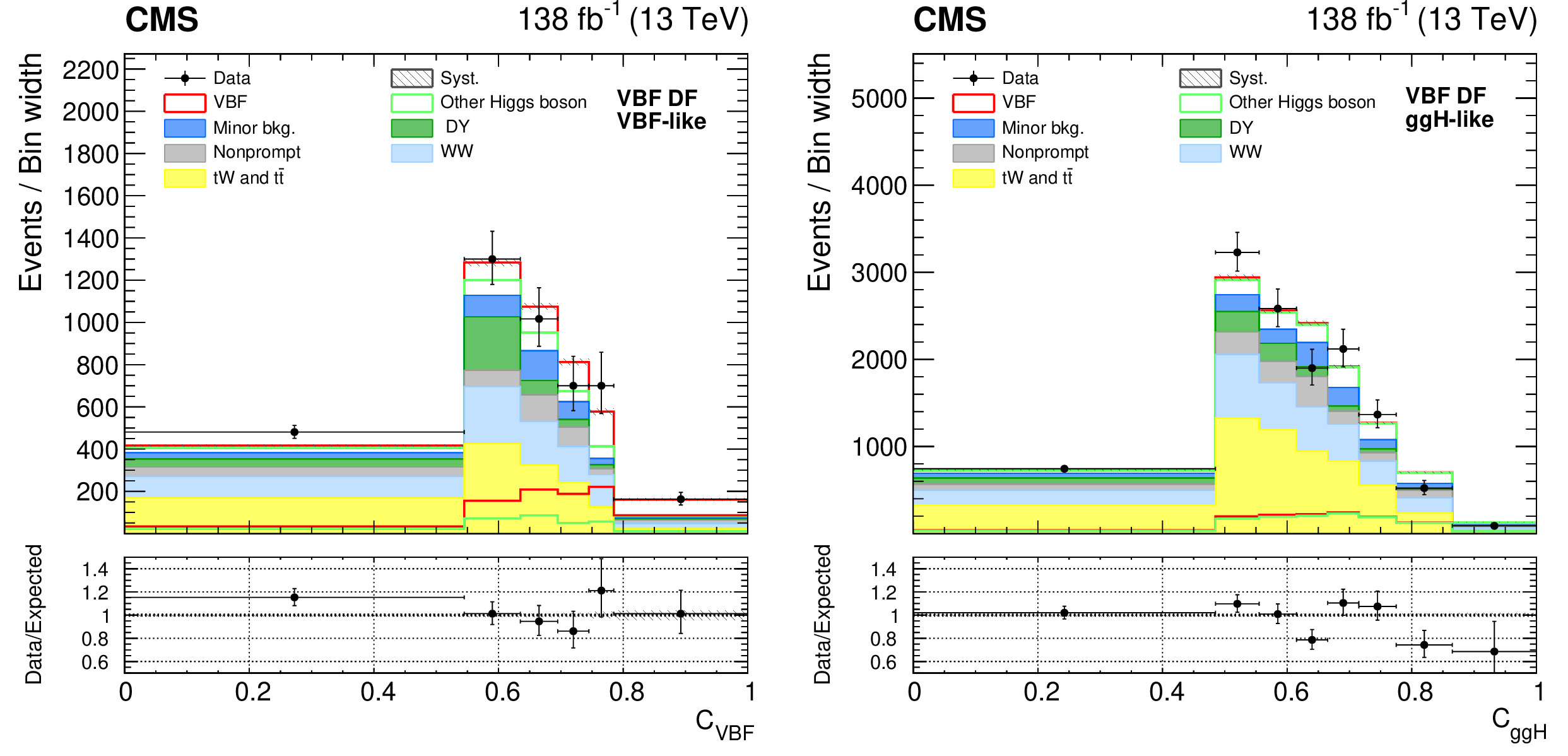
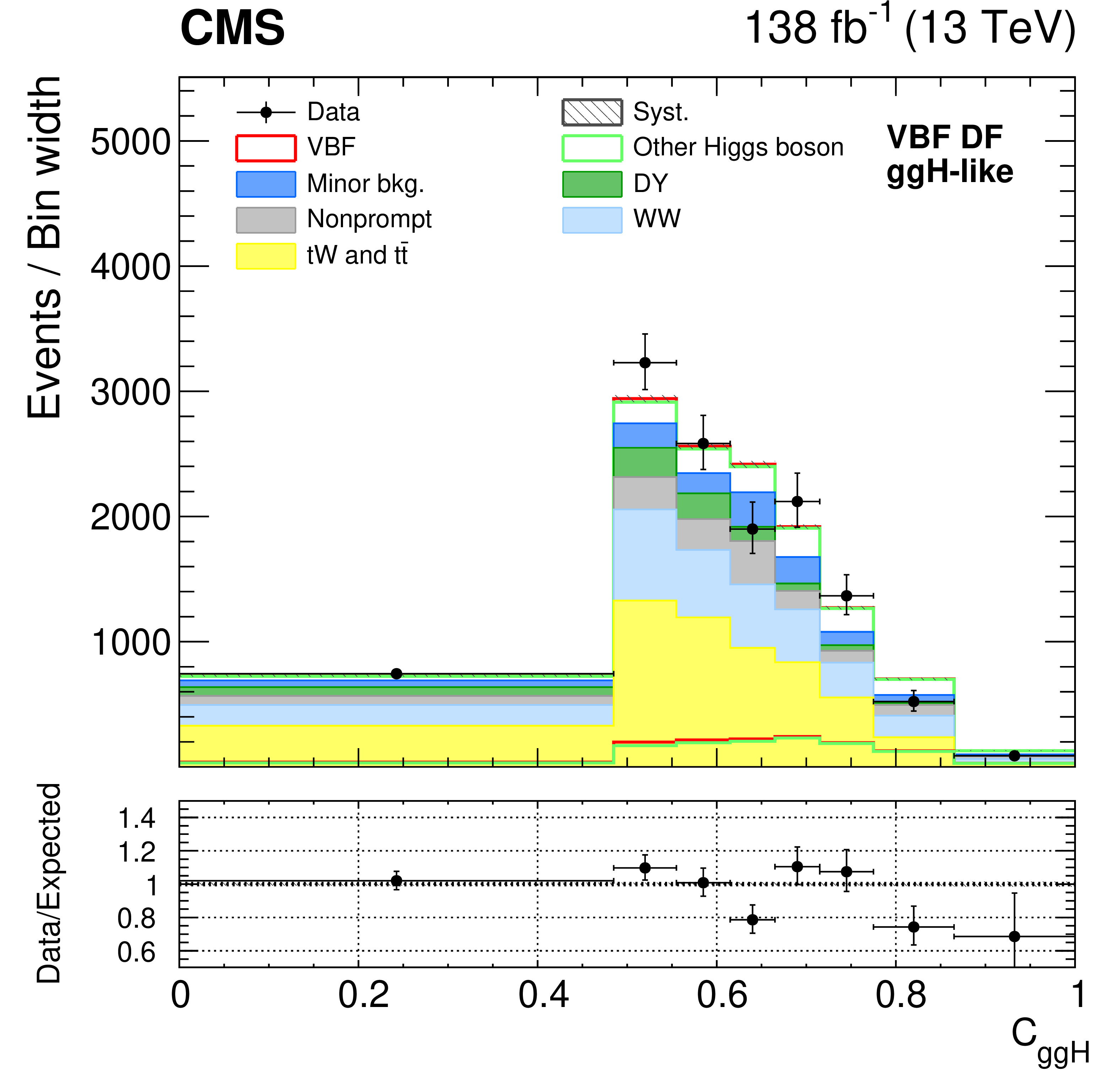
Figure 10:
Distributions for the $C_{\mathrm {VBF}}$ (left) and $C_{{\mathrm{g} \mathrm{g} \mathrm{H}}}$ (right) classifiers in the VBF-like and ggH-like VBF DF categories, respectively. A detailed description is given in the Fig. 1 caption. |

png pdf |
Figure 10-a:
Distributions for the $C_{\mathrm {VBF}}$ (left) and $C_{{\mathrm{g} \mathrm{g} \mathrm{H}}}$ (right) classifiers in the VBF-like and ggH-like VBF DF categories, respectively. A detailed description is given in the Fig. 1 caption. |
png pdf |
Figure 10-b:
Distributions for the $C_{\mathrm {VBF}}$ (left) and $C_{{\mathrm{g} \mathrm{g} \mathrm{H}}}$ (right) classifiers in the VBF-like and ggH-like VBF DF categories, respectively. A detailed description is given in the Fig. 1 caption. |
png pdf |
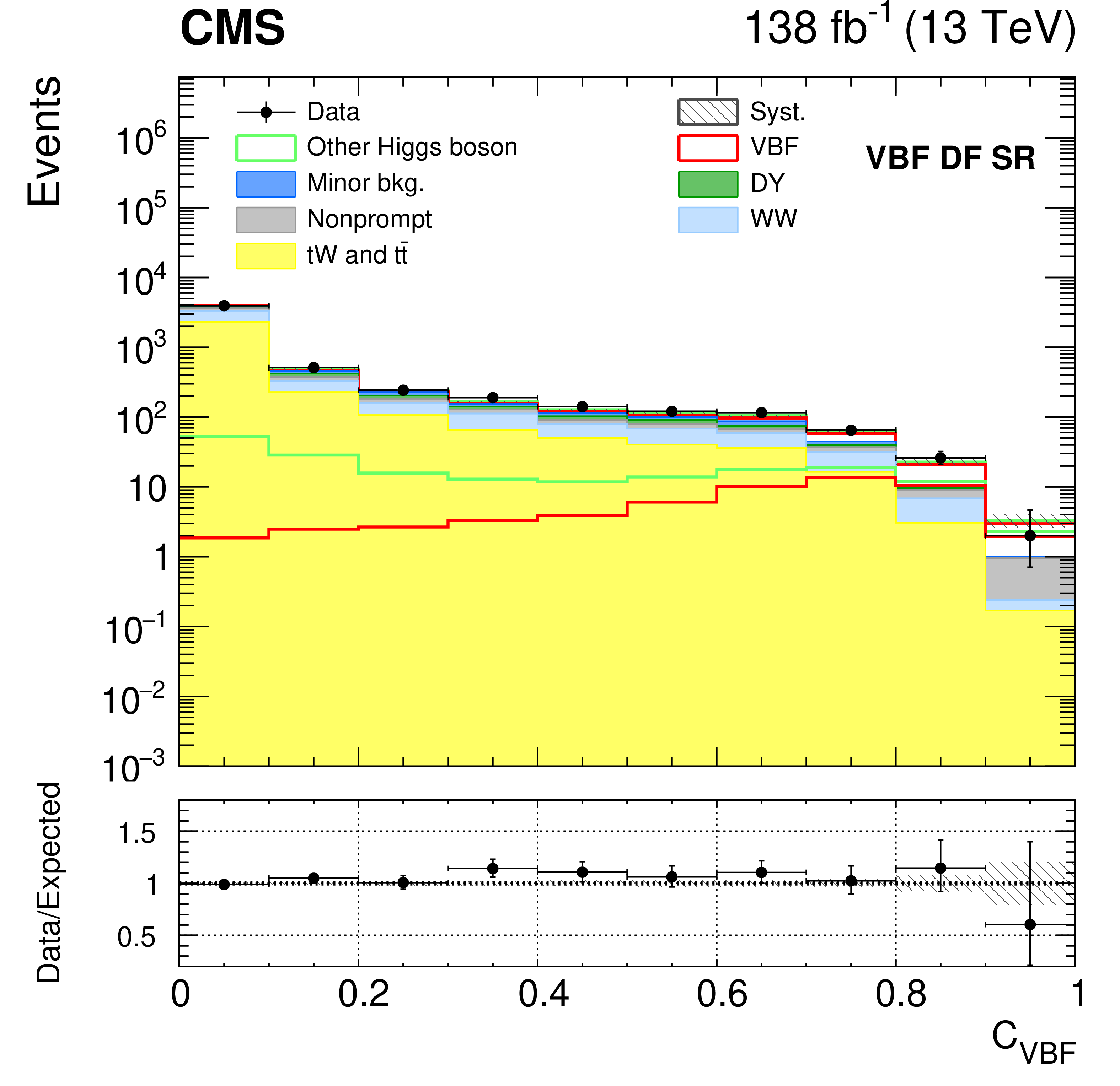
Figure 11:
Distribution of the $C_{\mathrm {VBF}}$ classifier in the VBF DF SR, before the further event categorization based on the classifier outputs. A detailed description is given in the Fig. 1 caption. |
png pdf |
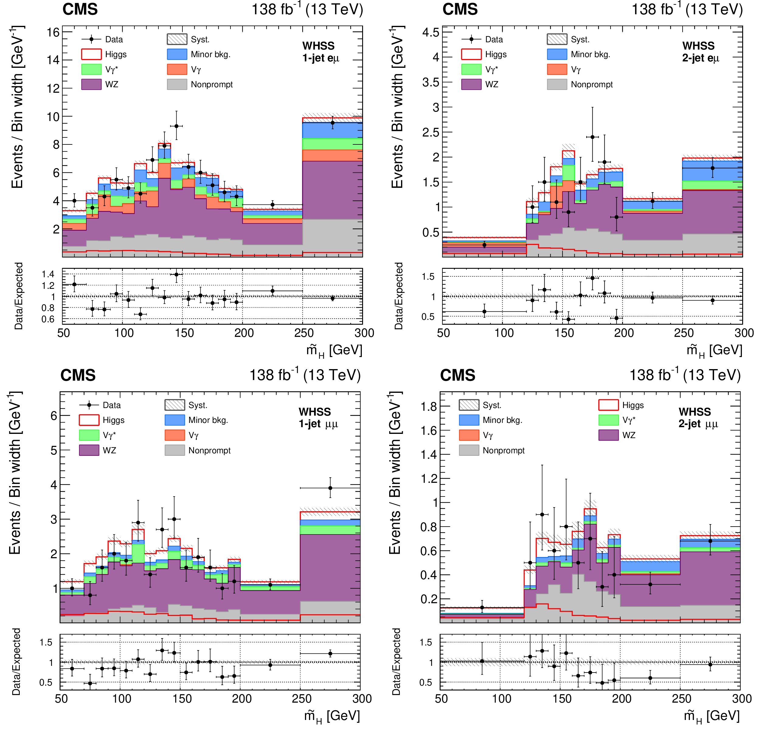
Figure 12:
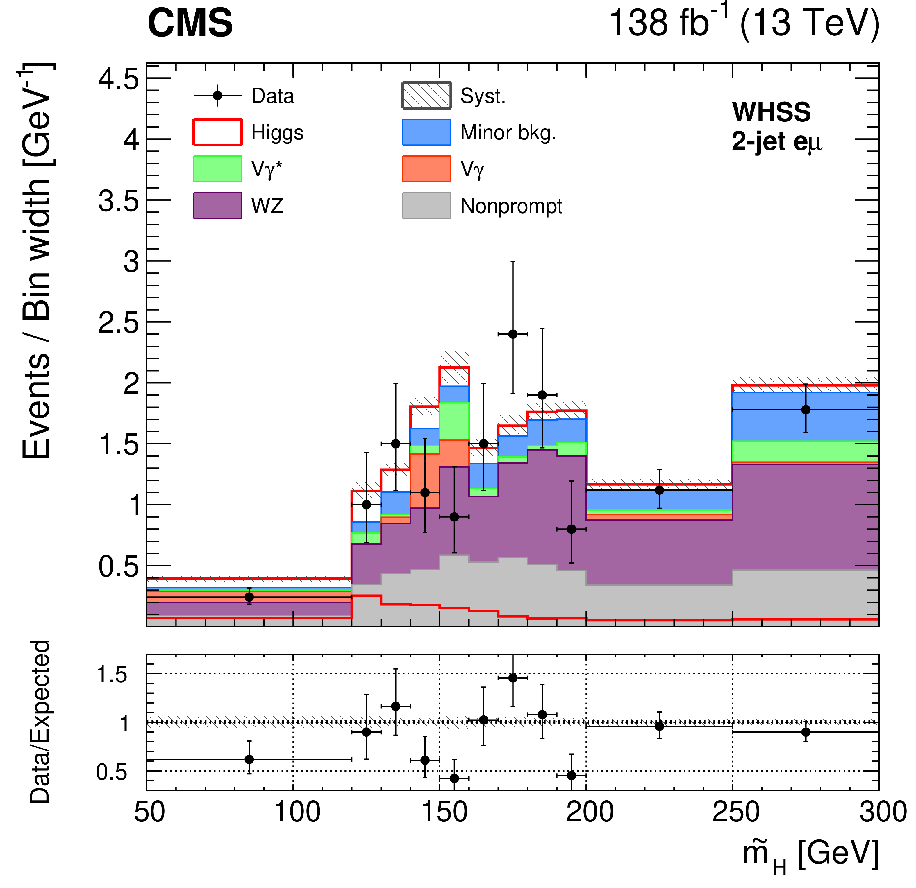
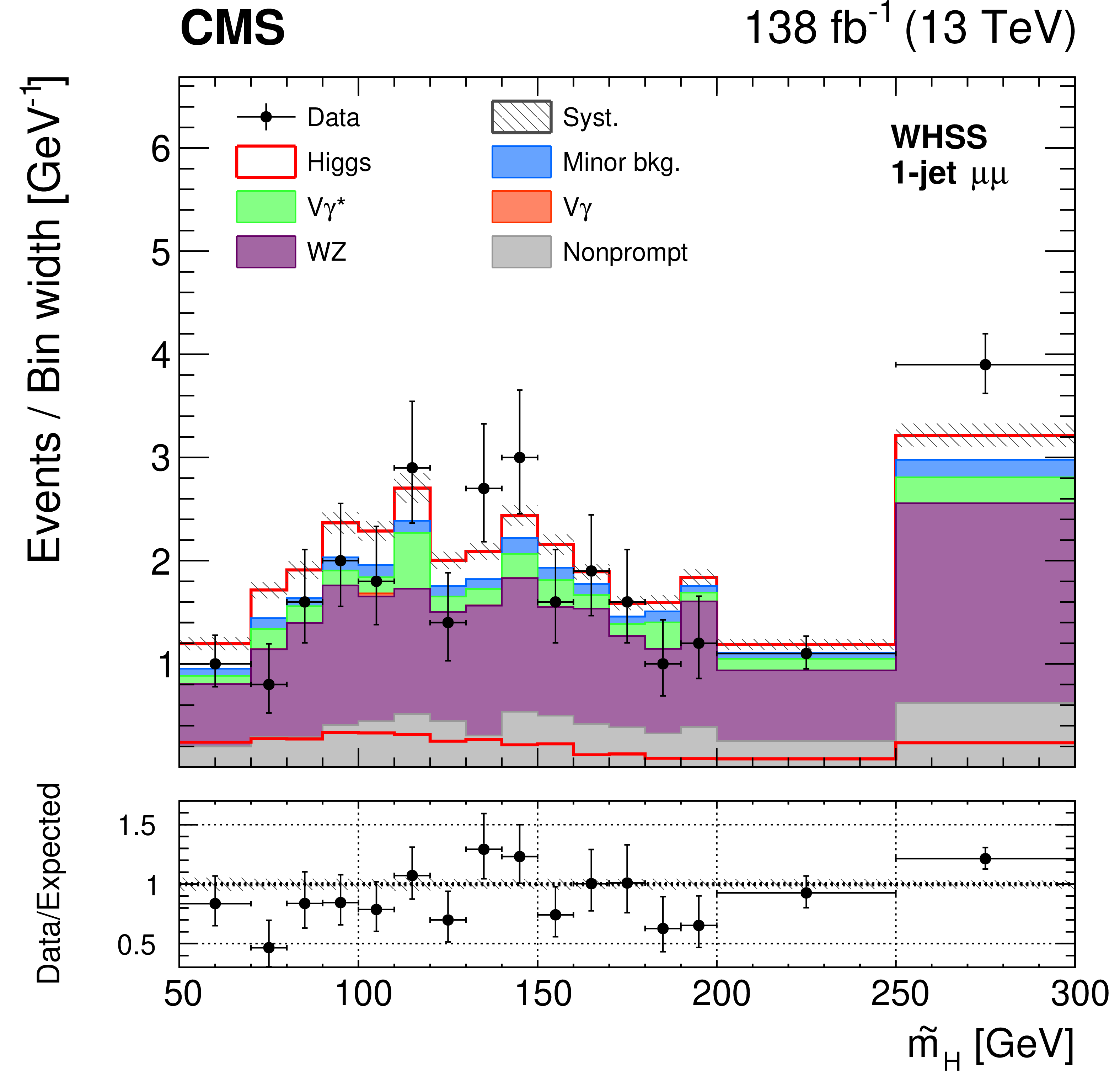
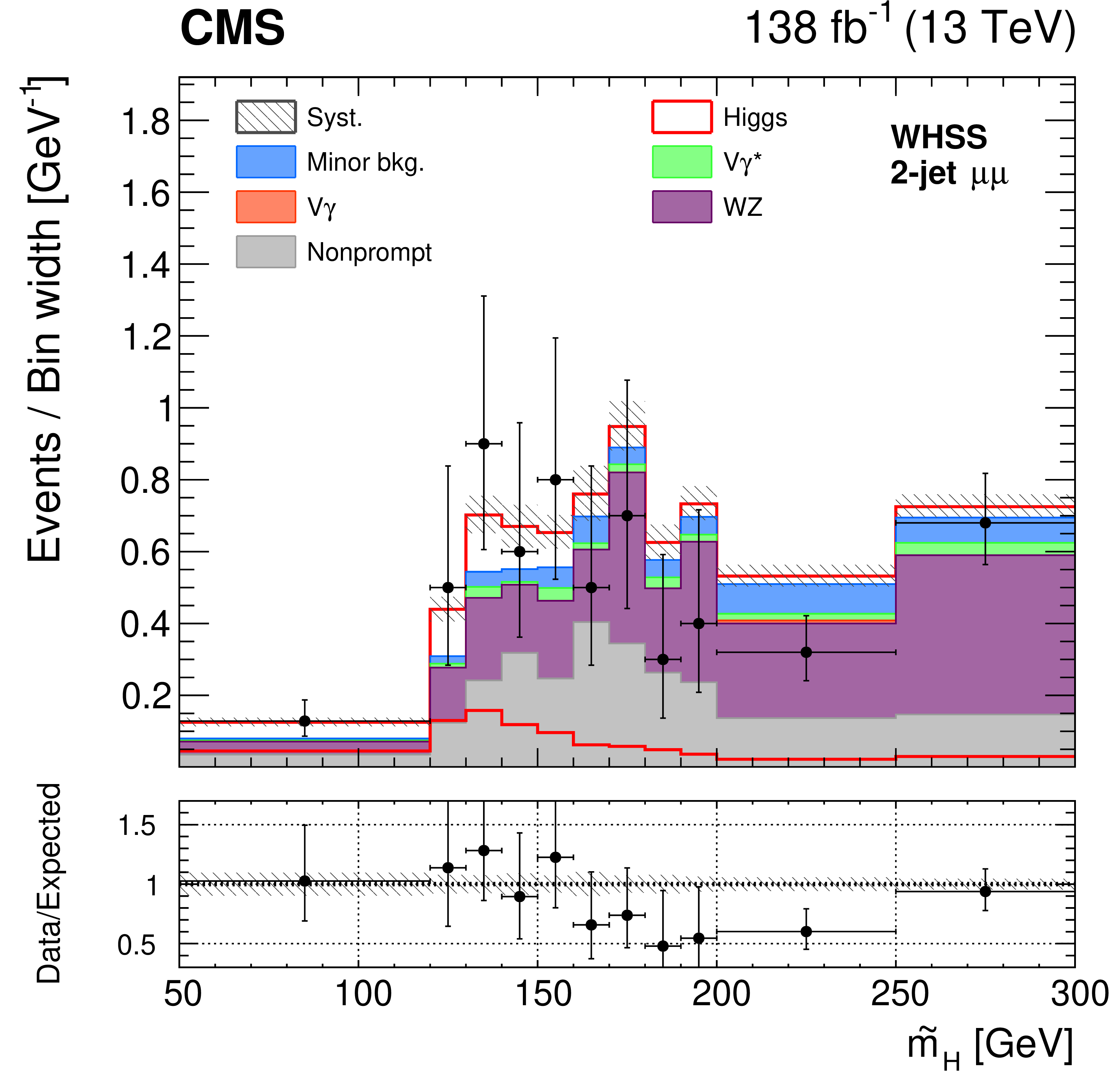
Observed distributions of the ${\tilde{m}_{\mathrm{H}}}$ fit variable in the WHSS 1-jet e${\mu}$(upper left), 2-jet e${\mu}$(upper right), 1-jet ${\mu}{\mu}$ (lower left), and 2-jet ${\mu}{\mu}$ (lower right) SRs. A detailed description is given in the Fig. 1 caption. |
png pdf |
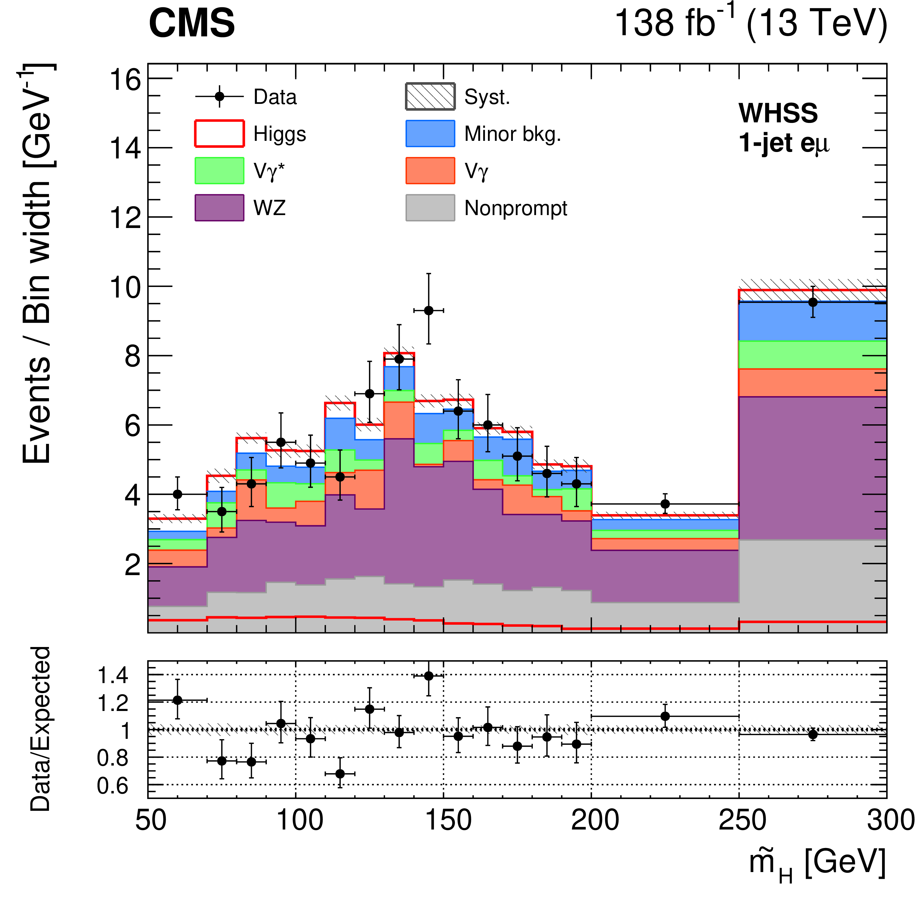
Figure 12-a:
Observed distributions of the ${\tilde{m}_{\mathrm{H}}}$ fit variable in the WHSS 1-jet e${\mu}$(upper left), 2-jet e${\mu}$(upper right), 1-jet ${\mu}{\mu}$ (lower left), and 2-jet ${\mu}{\mu}$ (lower right) SRs. A detailed description is given in the Fig. 1 caption. |
png pdf |
Figure 12-b:
Observed distributions of the ${\tilde{m}_{\mathrm{H}}}$ fit variable in the WHSS 1-jet e${\mu}$(upper left), 2-jet e${\mu}$(upper right), 1-jet ${\mu}{\mu}$ (lower left), and 2-jet ${\mu}{\mu}$ (lower right) SRs. A detailed description is given in the Fig. 1 caption. |
png pdf |
Figure 12-c:
Observed distributions of the ${\tilde{m}_{\mathrm{H}}}$ fit variable in the WHSS 1-jet e${\mu}$(upper left), 2-jet e${\mu}$(upper right), 1-jet ${\mu}{\mu}$ (lower left), and 2-jet ${\mu}{\mu}$ (lower right) SRs. A detailed description is given in the Fig. 1 caption. |
png pdf |
Figure 12-d:
Observed distributions of the ${\tilde{m}_{\mathrm{H}}}$ fit variable in the WHSS 1-jet e${\mu}$(upper left), 2-jet e${\mu}$(upper right), 1-jet ${\mu}{\mu}$ (lower left), and 2-jet ${\mu}{\mu}$ (lower right) SRs. A detailed description is given in the Fig. 1 caption. |
png pdf |
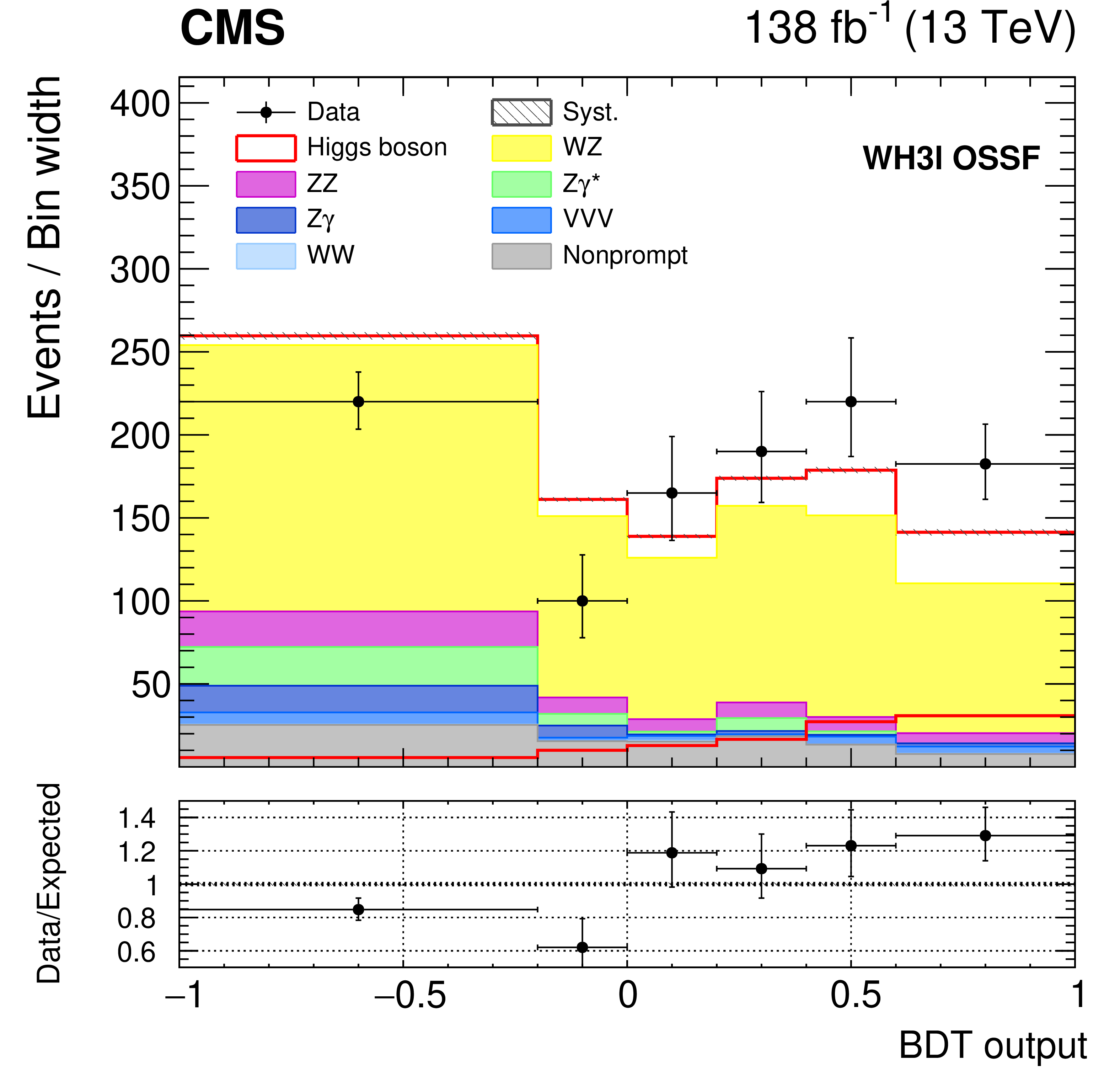
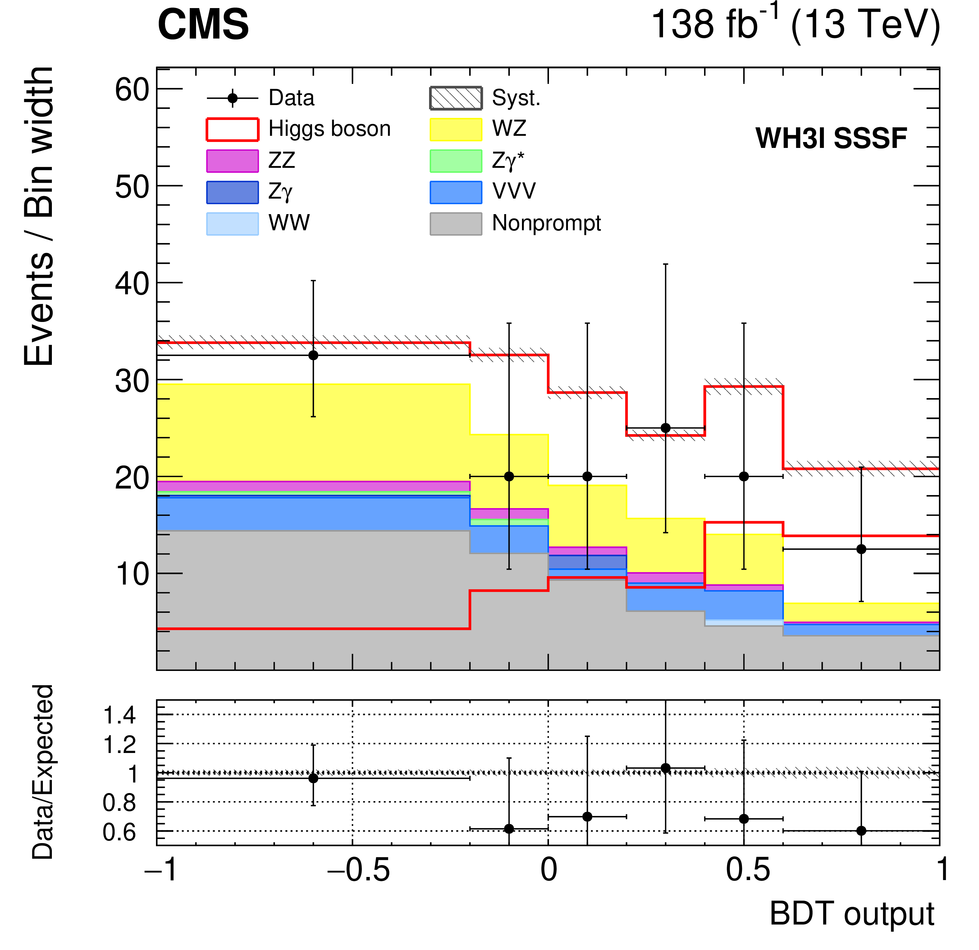
Figure 13:
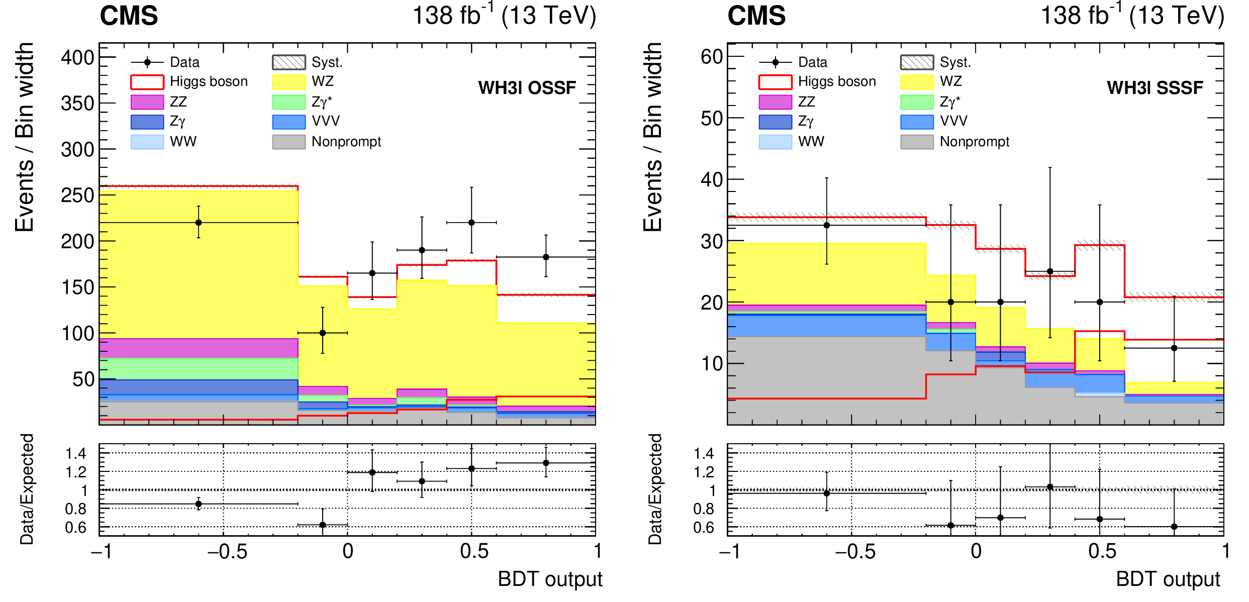
Observed distributions of the BDT score in the WH3$\ell$ OSSF (left) and SSSF (right) SRs. A detailed description is given in the Fig. 1 caption. |
png pdf |
Figure 13-a:
Observed distributions of the BDT score in the WH3$\ell$ OSSF (left) and SSSF (right) SRs. A detailed description is given in the Fig. 1 caption. |
png pdf |
Figure 13-b:
Observed distributions of the BDT score in the WH3$\ell$ OSSF (left) and SSSF (right) SRs. A detailed description is given in the Fig. 1 caption. |
png pdf |
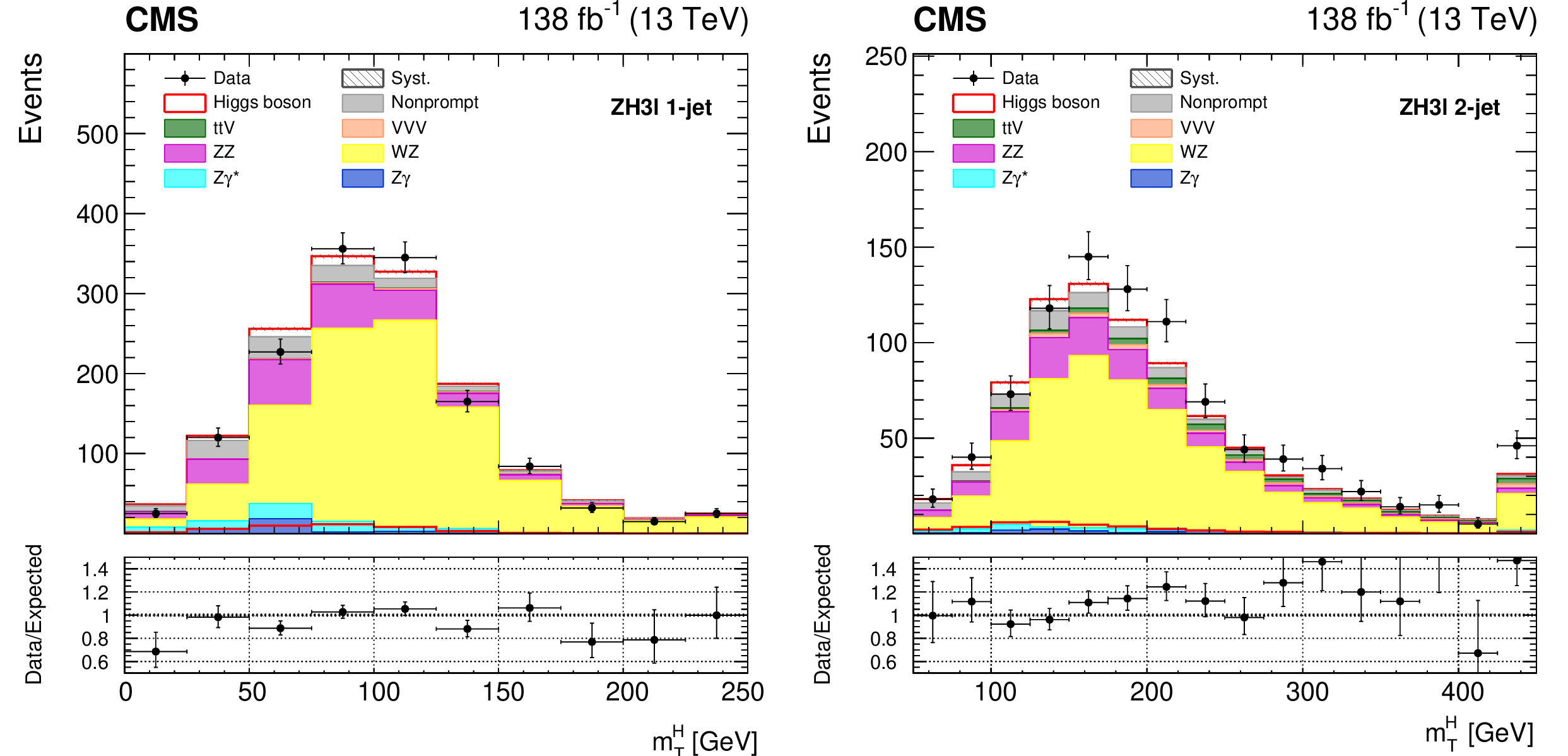
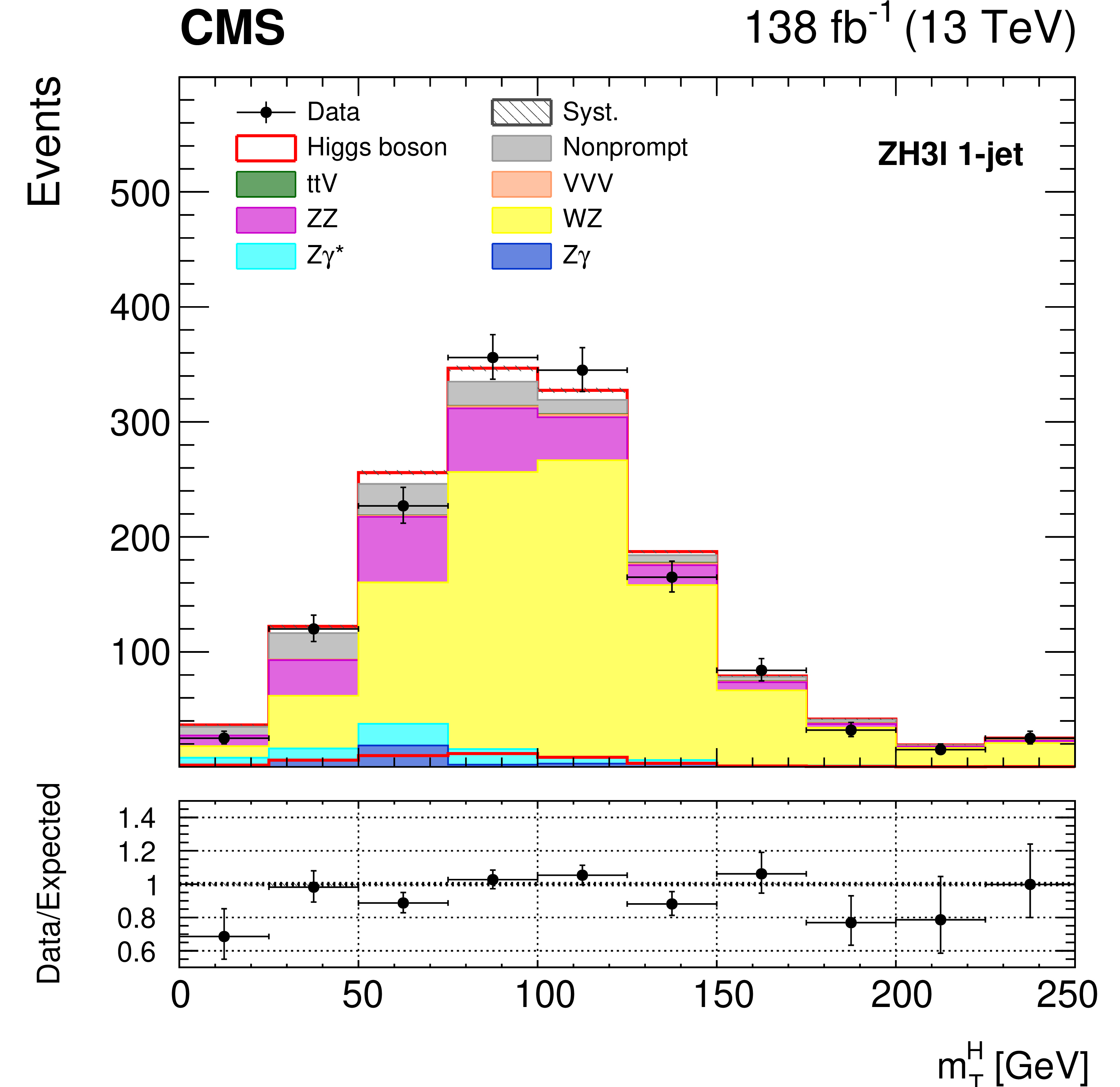
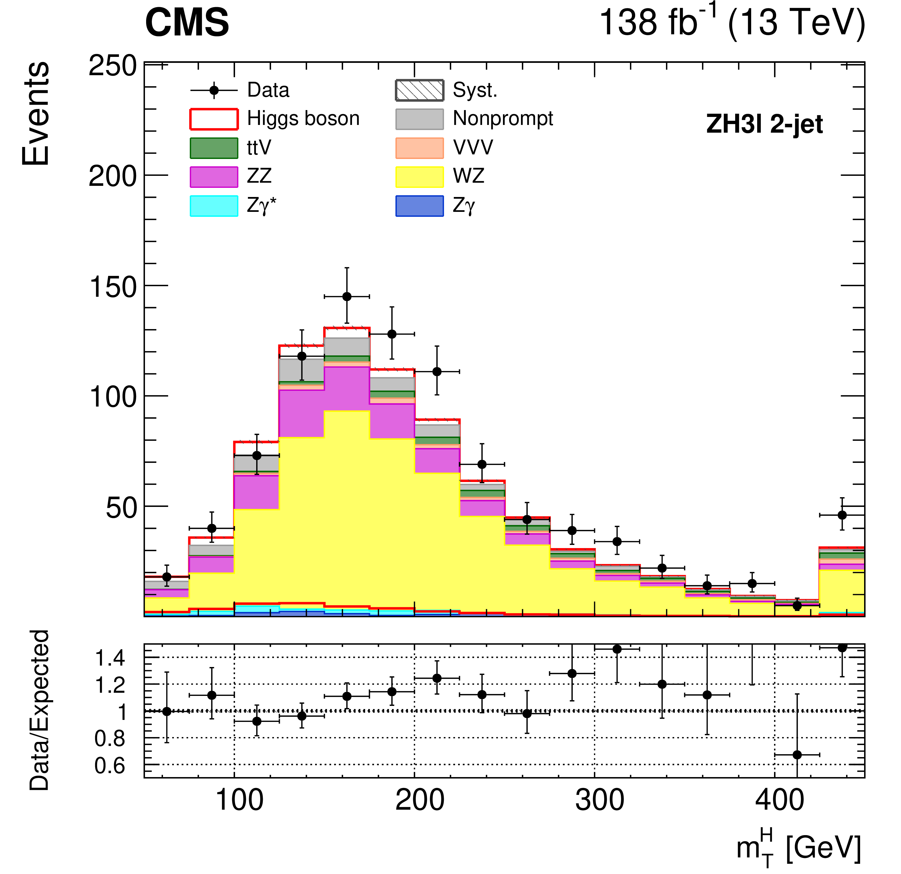
Figure 14:
Observed distributions of the ${{m_{\mathrm {T}}} ^{\mathrm{H}}}$ fit variable in the ZH3$\ell$ 1-jet (left) and 2-jet (right) SRs. A detailed description is given in the Fig. 1 caption. |
png pdf |
Figure 14-a:
Observed distributions of the ${{m_{\mathrm {T}}} ^{\mathrm{H}}}$ fit variable in the ZH3$\ell$ 1-jet (left) and 2-jet (right) SRs. A detailed description is given in the Fig. 1 caption. |
png pdf |
Figure 14-b:
Observed distributions of the ${{m_{\mathrm {T}}} ^{\mathrm{H}}}$ fit variable in the ZH3$\ell$ 1-jet (left) and 2-jet (right) SRs. A detailed description is given in the Fig. 1 caption. |
png pdf |
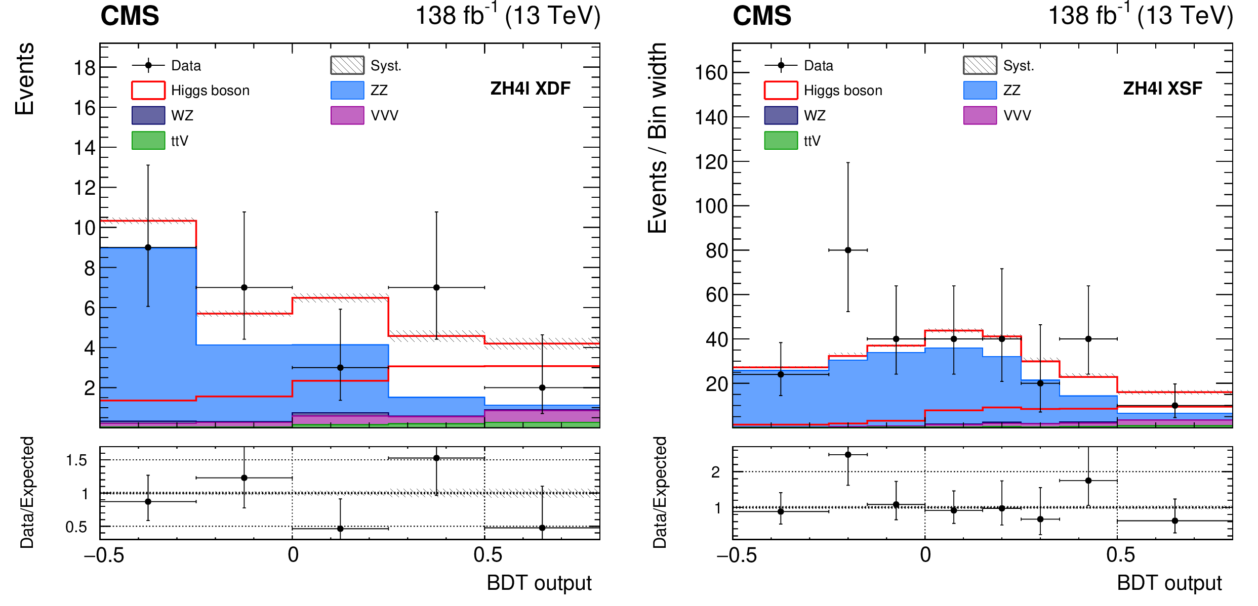
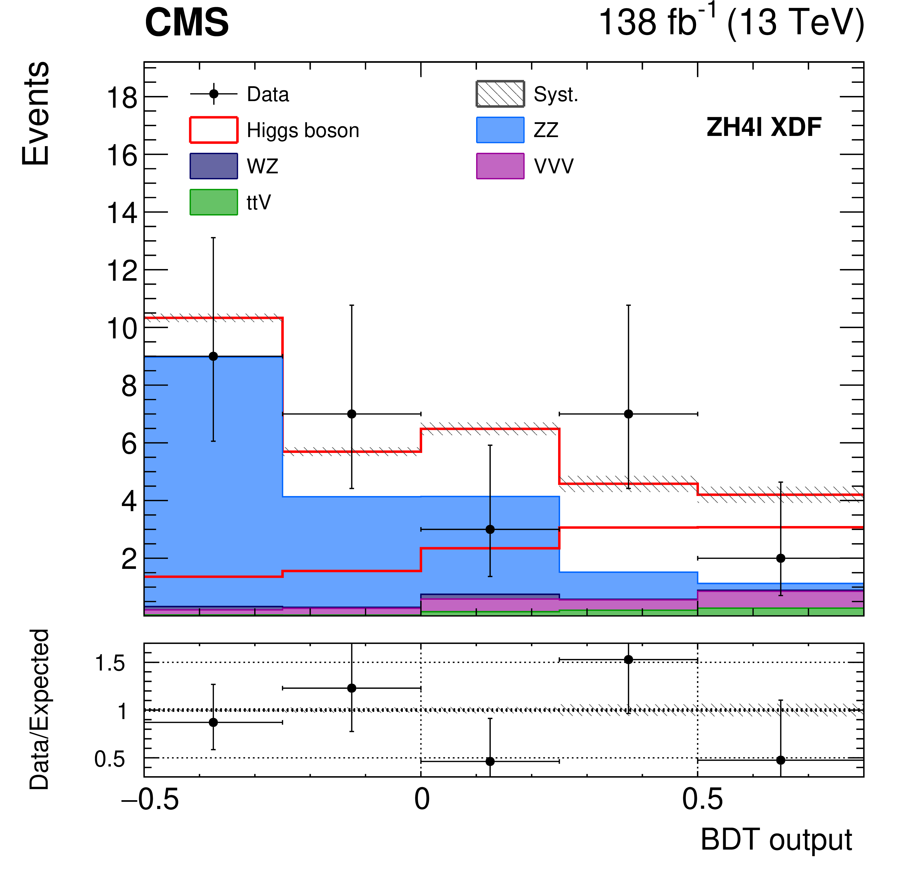
Figure 15:
Observed distributions of the BDT score in the ZH4$\ell$ XDF (left) and XSF (right) SRs. A detailed description is given in the Fig. 1 caption. |
png pdf |
Figure 15-a:
Observed distributions of the BDT score in the ZH4$\ell$ XDF (left) and XSF (right) SRs. A detailed description is given in the Fig. 1 caption. |
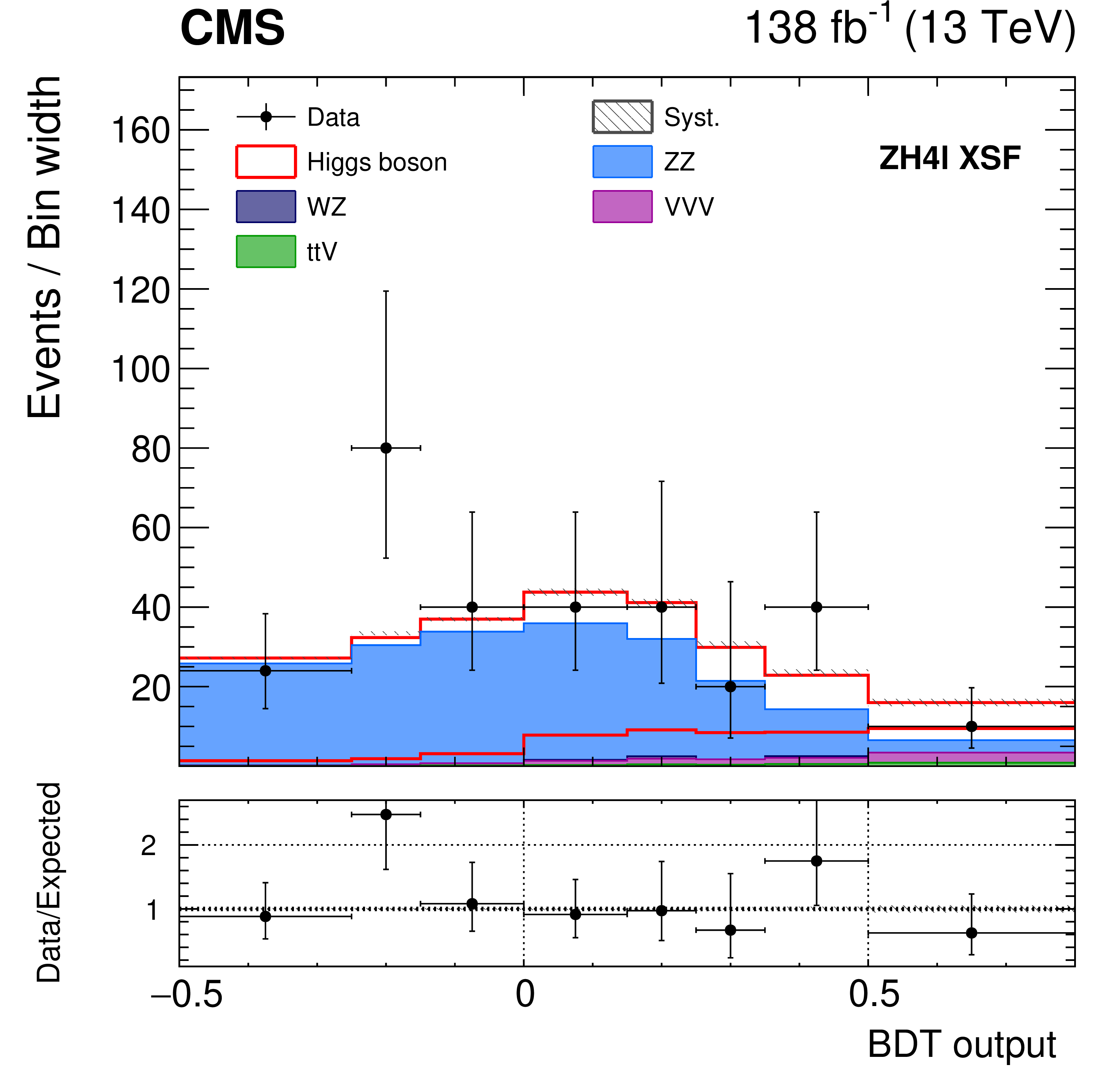
png pdf |
Figure 15-b:
Observed distributions of the BDT score in the ZH4$\ell$ XDF (left) and XSF (right) SRs. A detailed description is given in the Fig. 1 caption. |
png pdf |
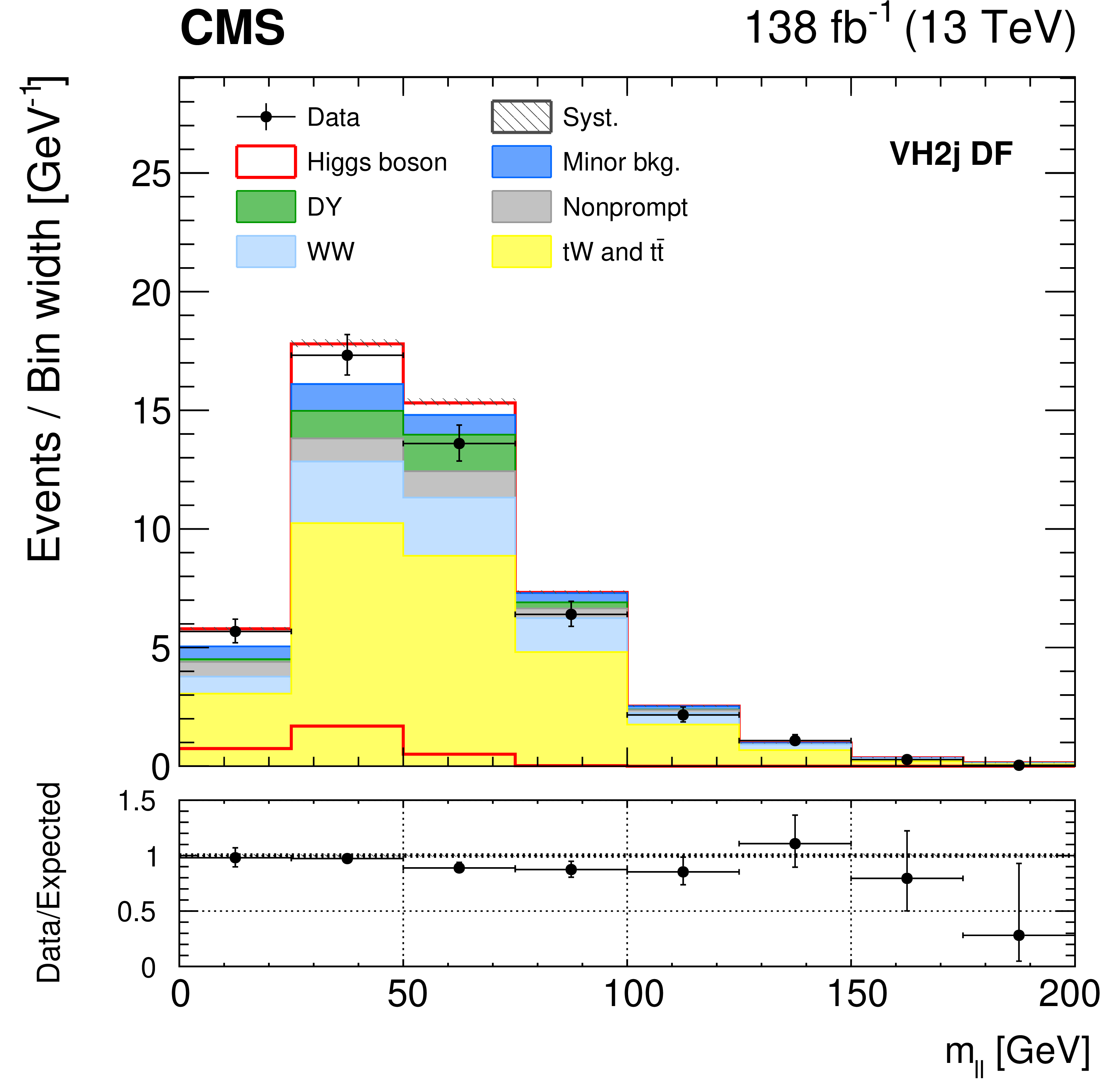
Figure 16:
Observed distribution of the ${m_{\ell \ell}}$ fit variable in the VH2j DF SR. A detailed description is given in the Fig. 1 caption. |
png pdf |
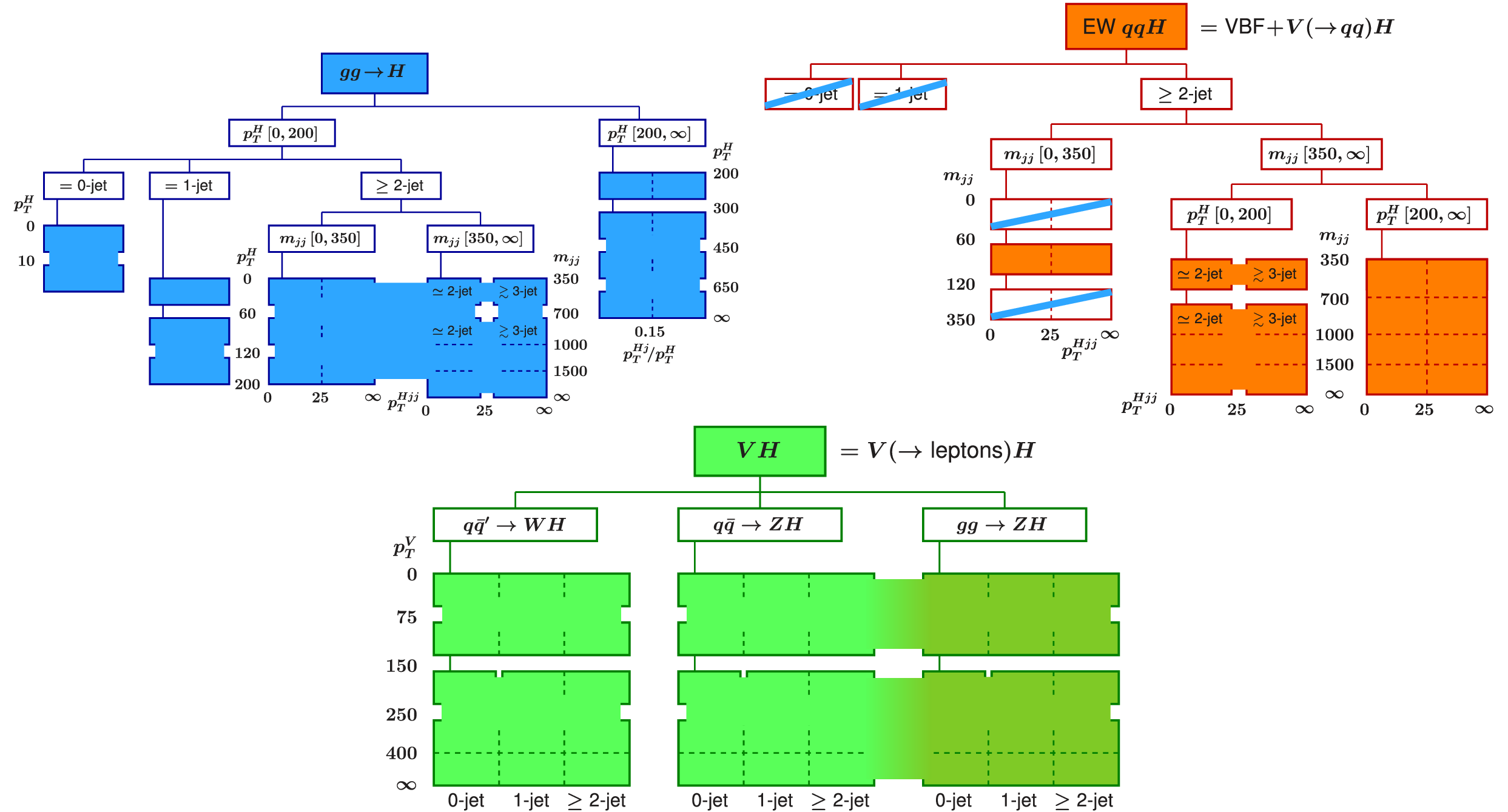
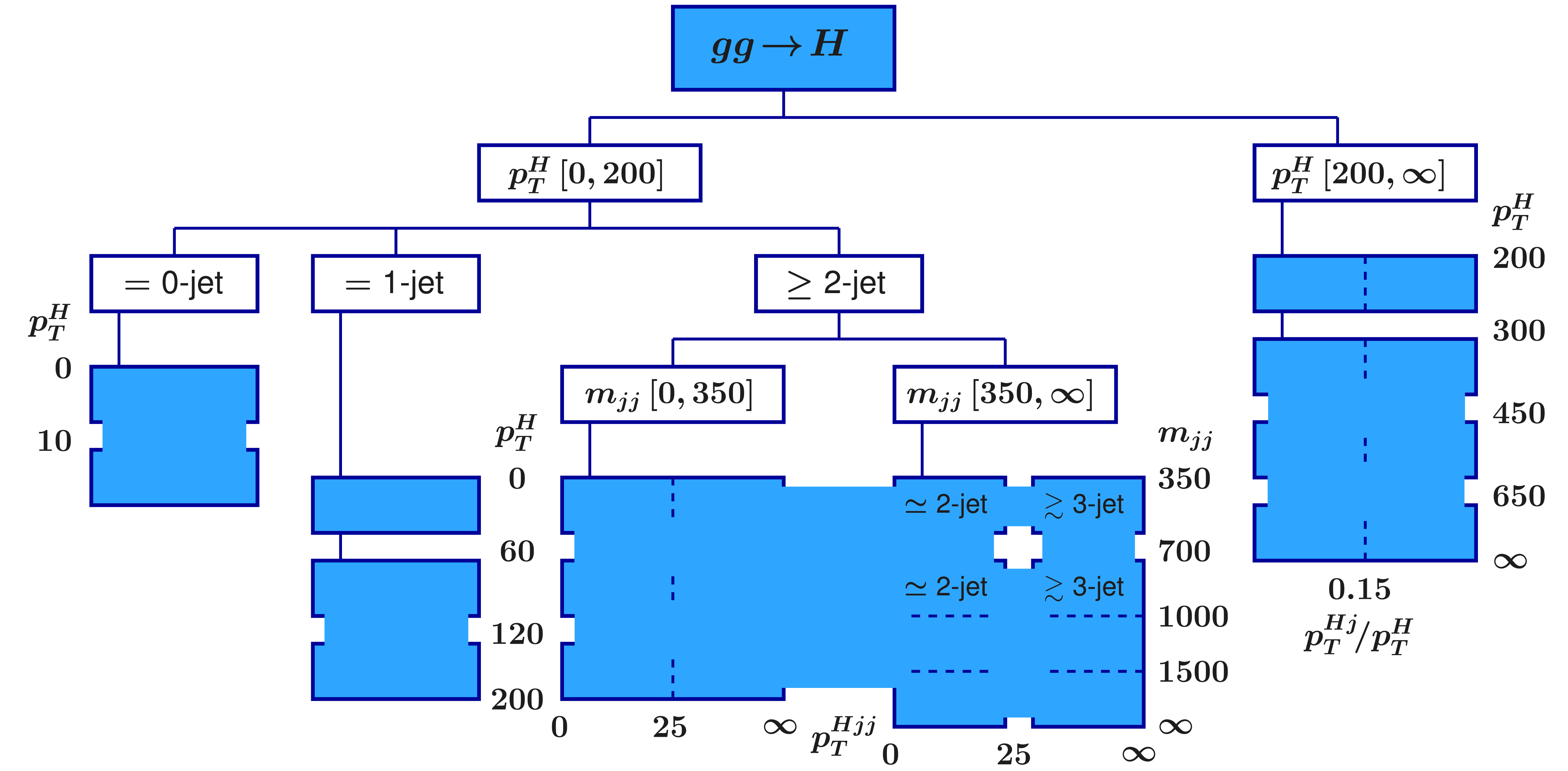
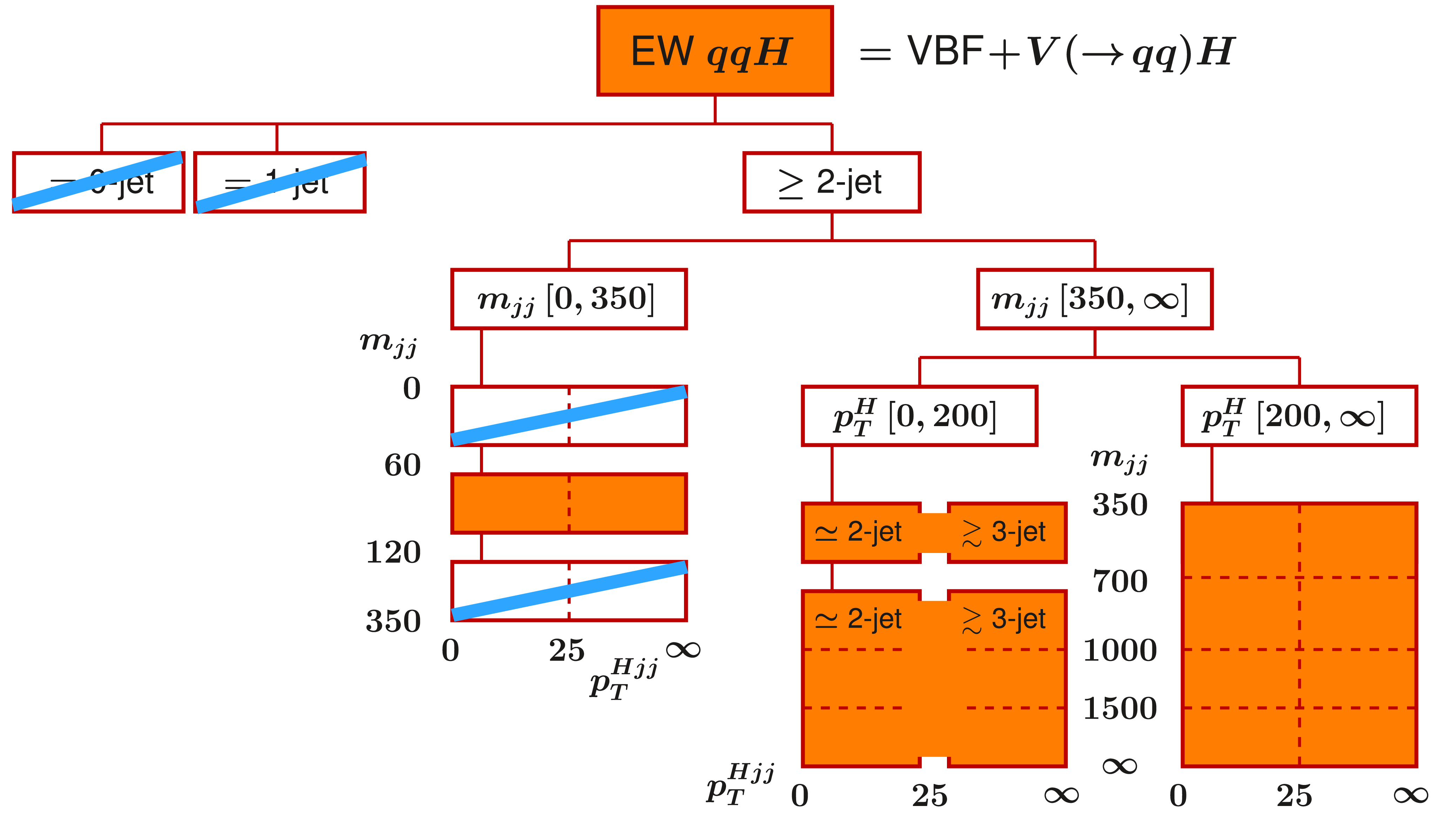
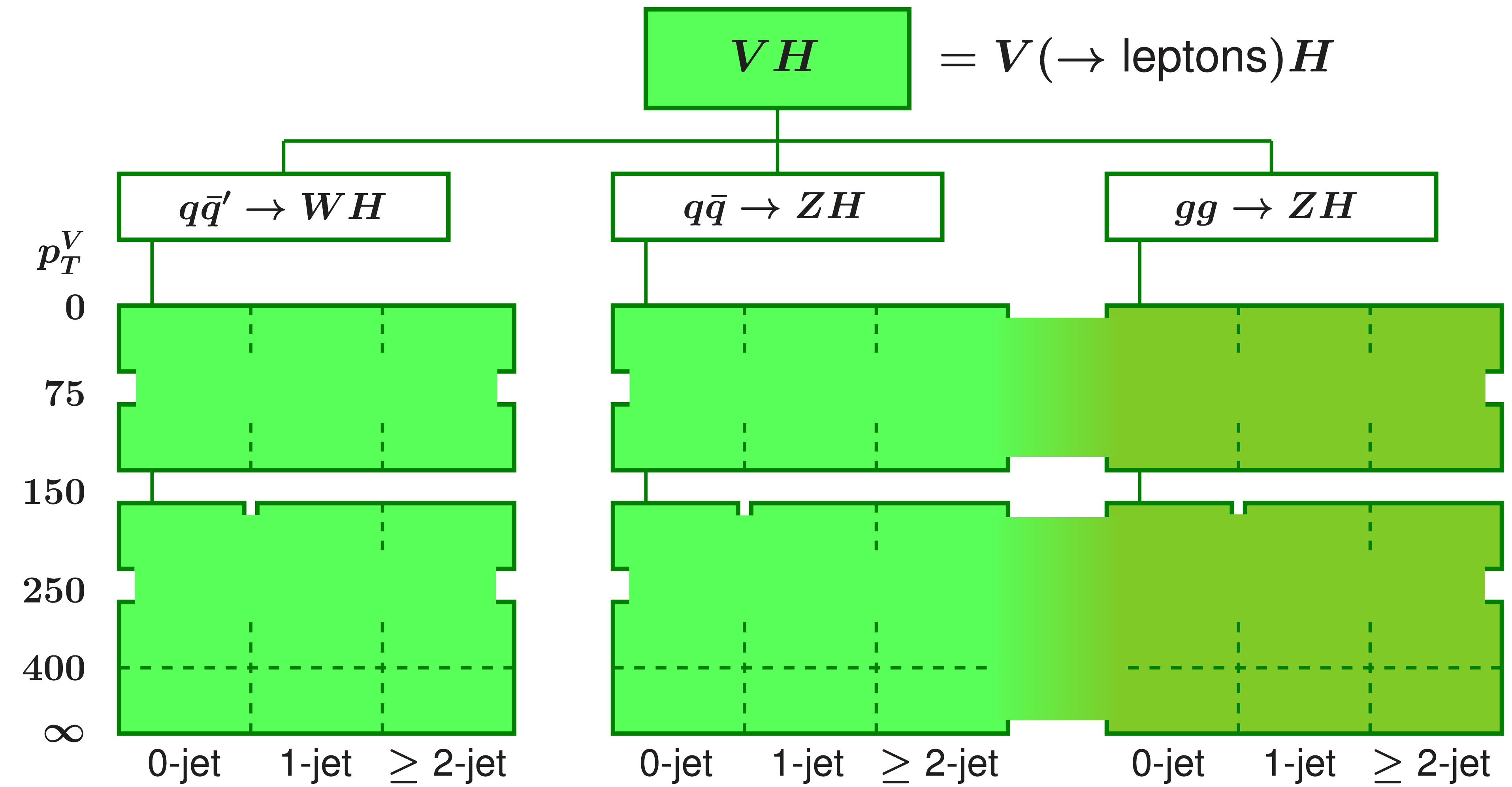
Figure 17:
The STXS Stage 1.2 binning scheme. Bins fused together with solid colors are measured as a single bin. |
png pdf |
Figure 17-a:
The STXS Stage 1.2 binning scheme. Bins fused together with solid colors are measured as a single bin. |
png pdf |
Figure 17-b:
The STXS Stage 1.2 binning scheme. Bins fused together with solid colors are measured as a single bin. |
png pdf |
Figure 17-c:
The STXS Stage 1.2 binning scheme. Bins fused together with solid colors are measured as a single bin. |
png pdf |
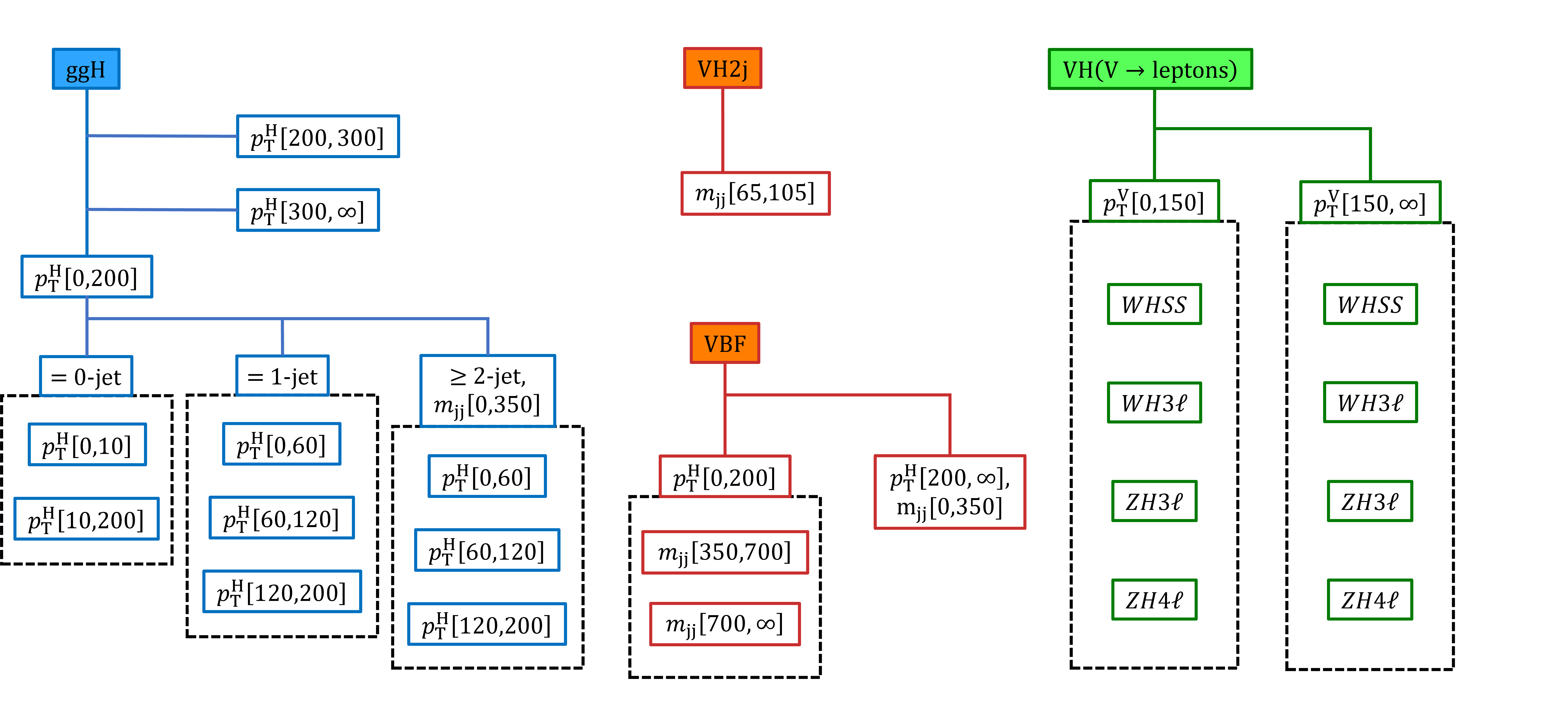
Figure 18:
Analysis categories targeting the STXS bins. The baseline ggH, VBF, and VH selections are identical to what was described in Sections 5-7. All dimensional quantities are measured in GeV. |
png pdf |
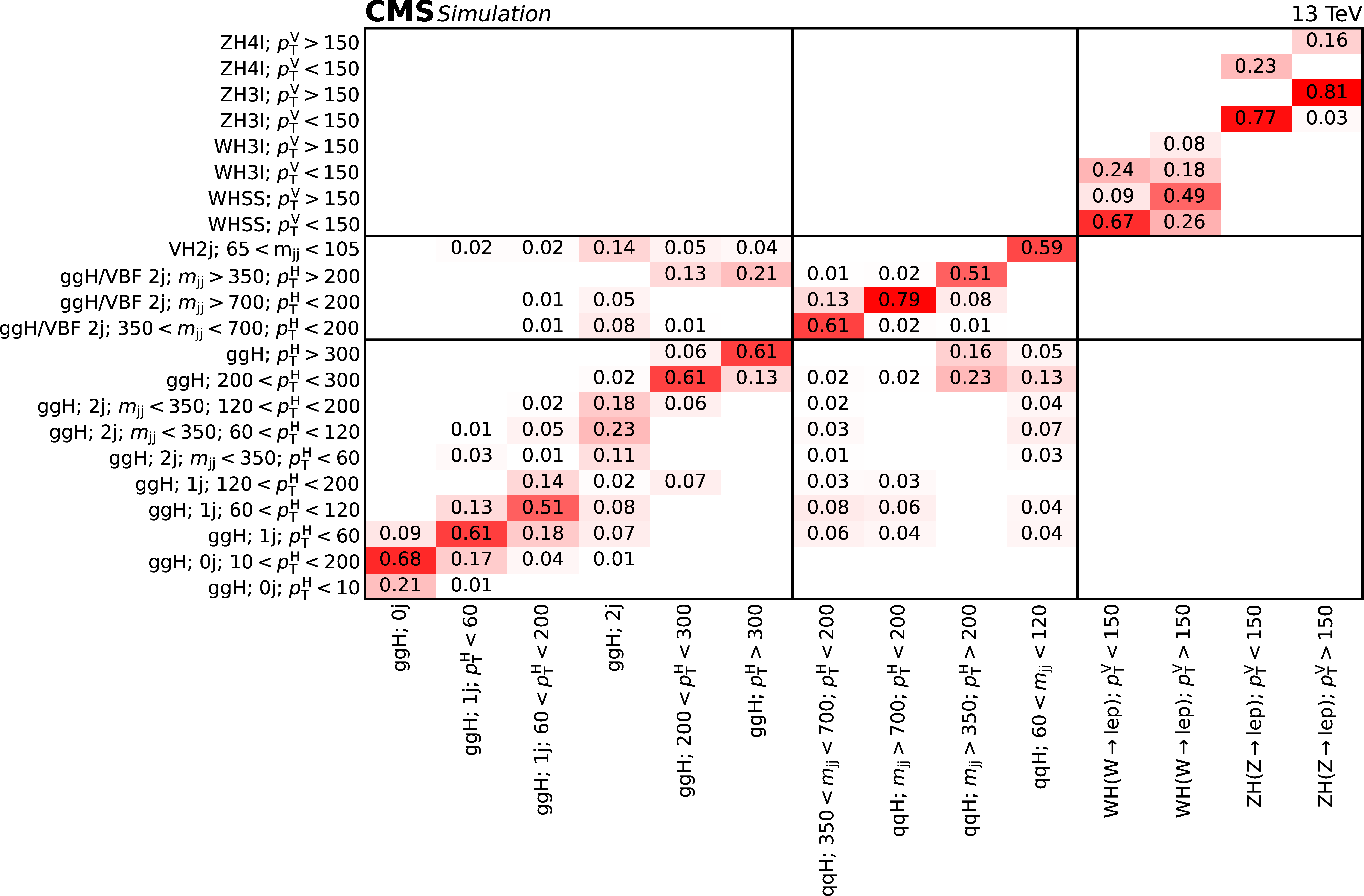
Figure 19:
Expected signal composition in each STXS bin. Generator-level bins are reported in the horizontal axis, and the corresponding analysis categories on the vertical axis. All quantities in the definitions of bins are measured in GeV. |
png pdf |
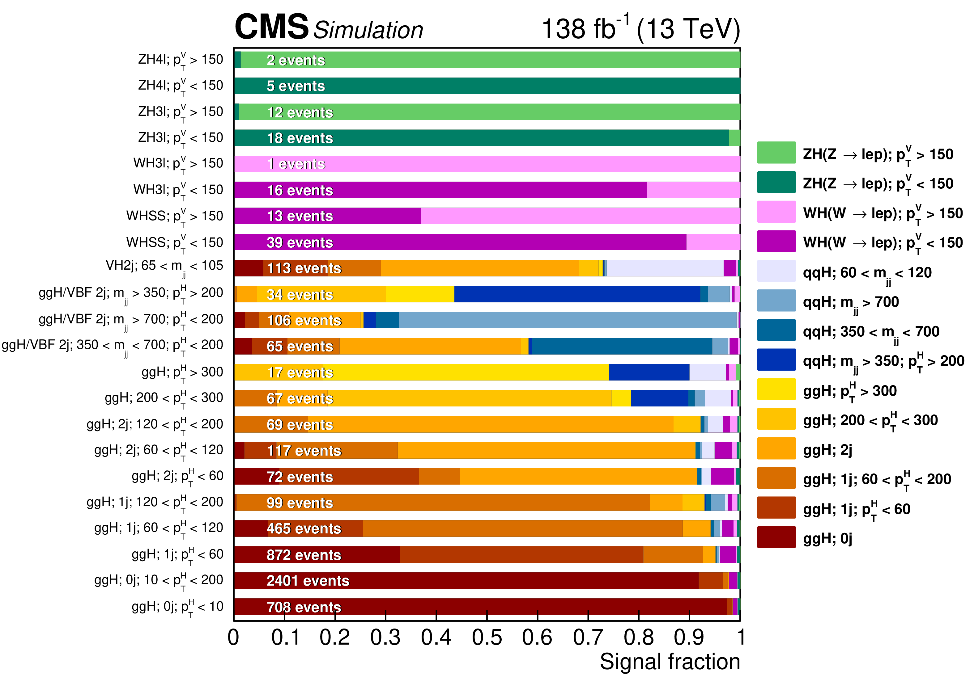
Figure 20:
Expected relative fractions of different STXS signal processes in each category. The total number of expected ${\mathrm{H} \to \mathrm{W} \mathrm{W}}$ signal events in each category is also shown. All dimensional quantities in the definitions of bins are measured in GeV. |
png pdf |
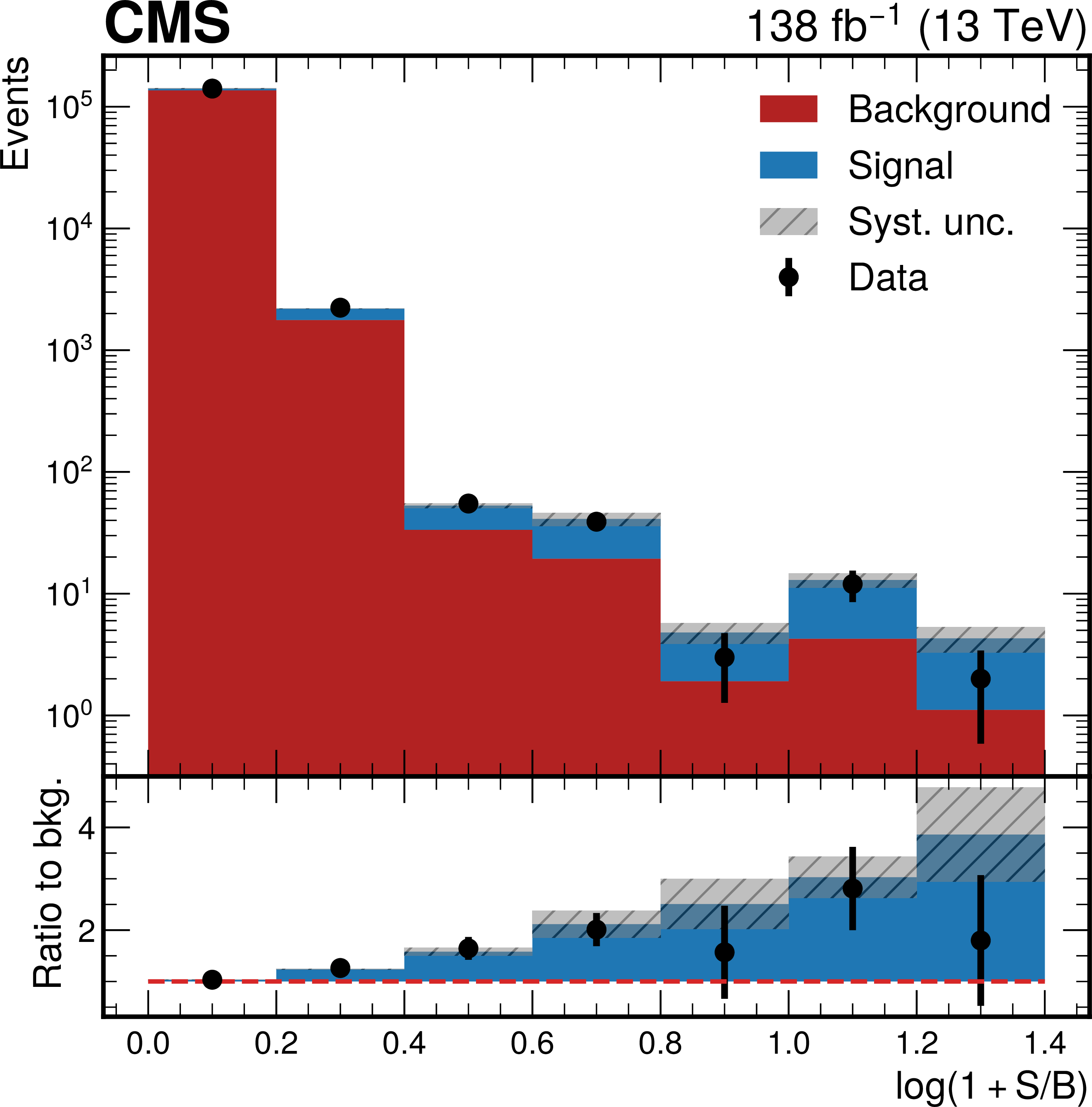
Figure 21:
Distribution of events as a function of the statistical significance of their corresponding bin in the analysis template, including all categories. Signal and background contributions are shown after the fit to the data. |

png pdf |
Figure 22:
Observed profile-likelihood function for the global signal strength modifier $\mu $. The dashed curve corresponds to the profile-likelihood function obtained considering statistical uncertainties only. |

png pdf |
Figure 23:
Observed signal strength modifiers for the main SM production modes. |
png pdf |
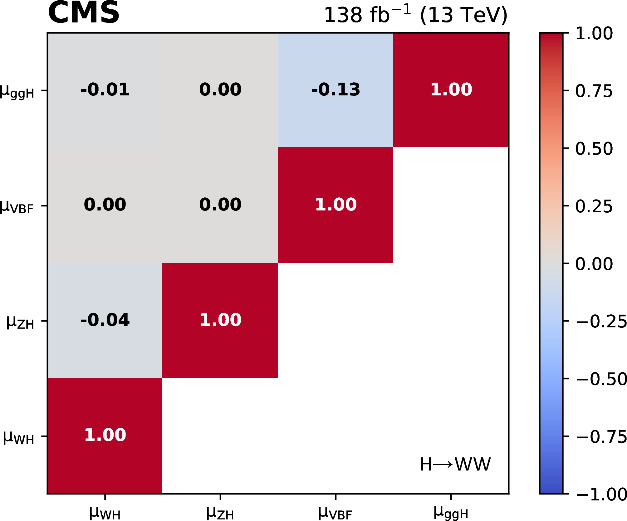
Figure 24:
Correlation matrix between the signal strength modifiers of the main production modes of the Higgs boson. |
png pdf |
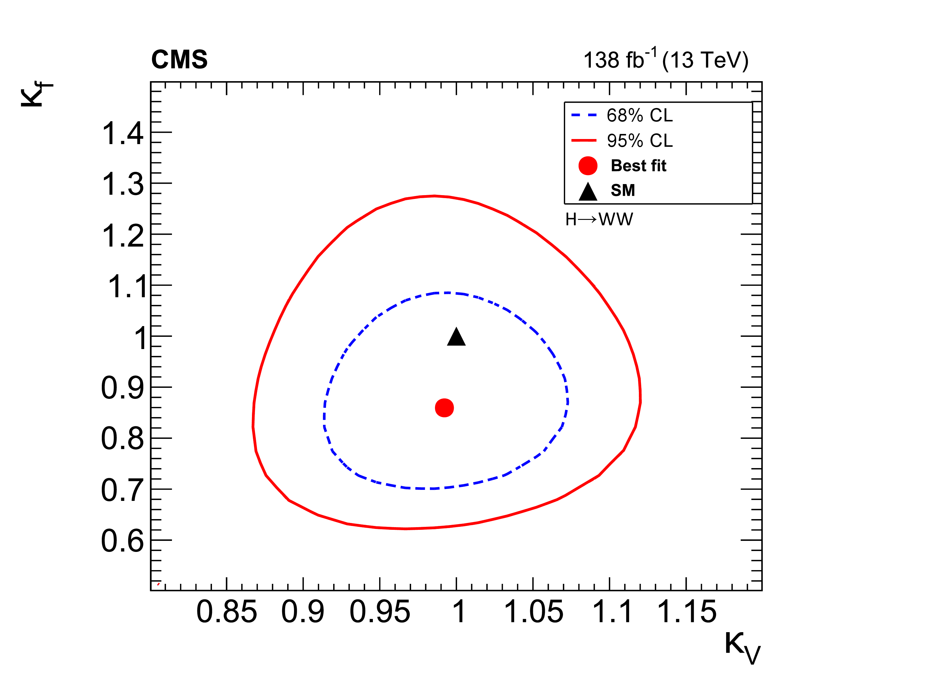
Figure 25:
Two-dimensional likelihood profile as a function of the coupling modifiers $\kappa _{{\mathrm{V}}}$ and $\kappa _\mathrm {f}$, using the $\kappa $-framework parametrization. The 95 and 68% confidence level contours are shown as continuous and dashed lines, respectively. |
png pdf |
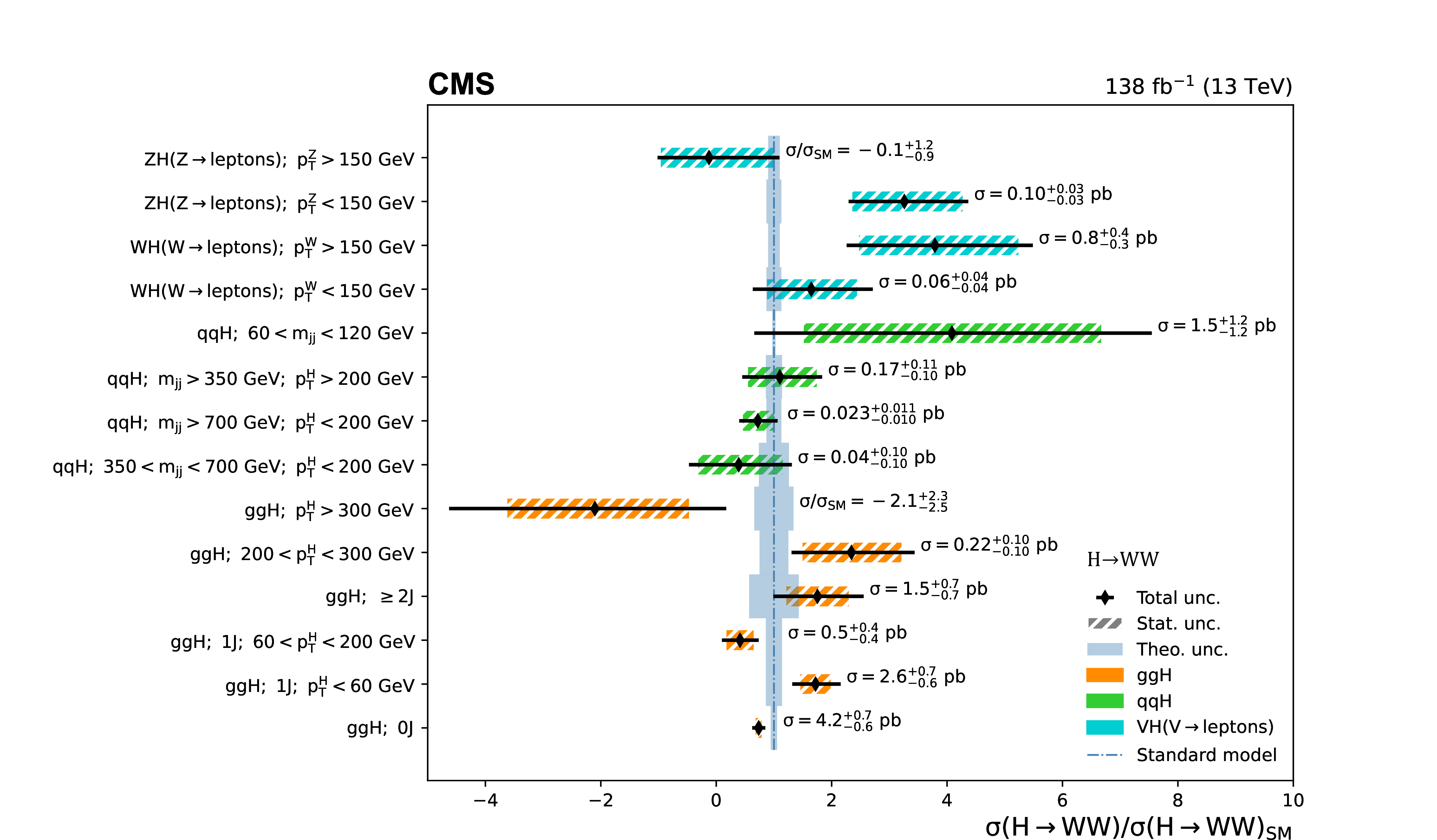
Figure 26:
Observed cross sections in each STXS bin, normalized to the SM expectation. |
png pdf |
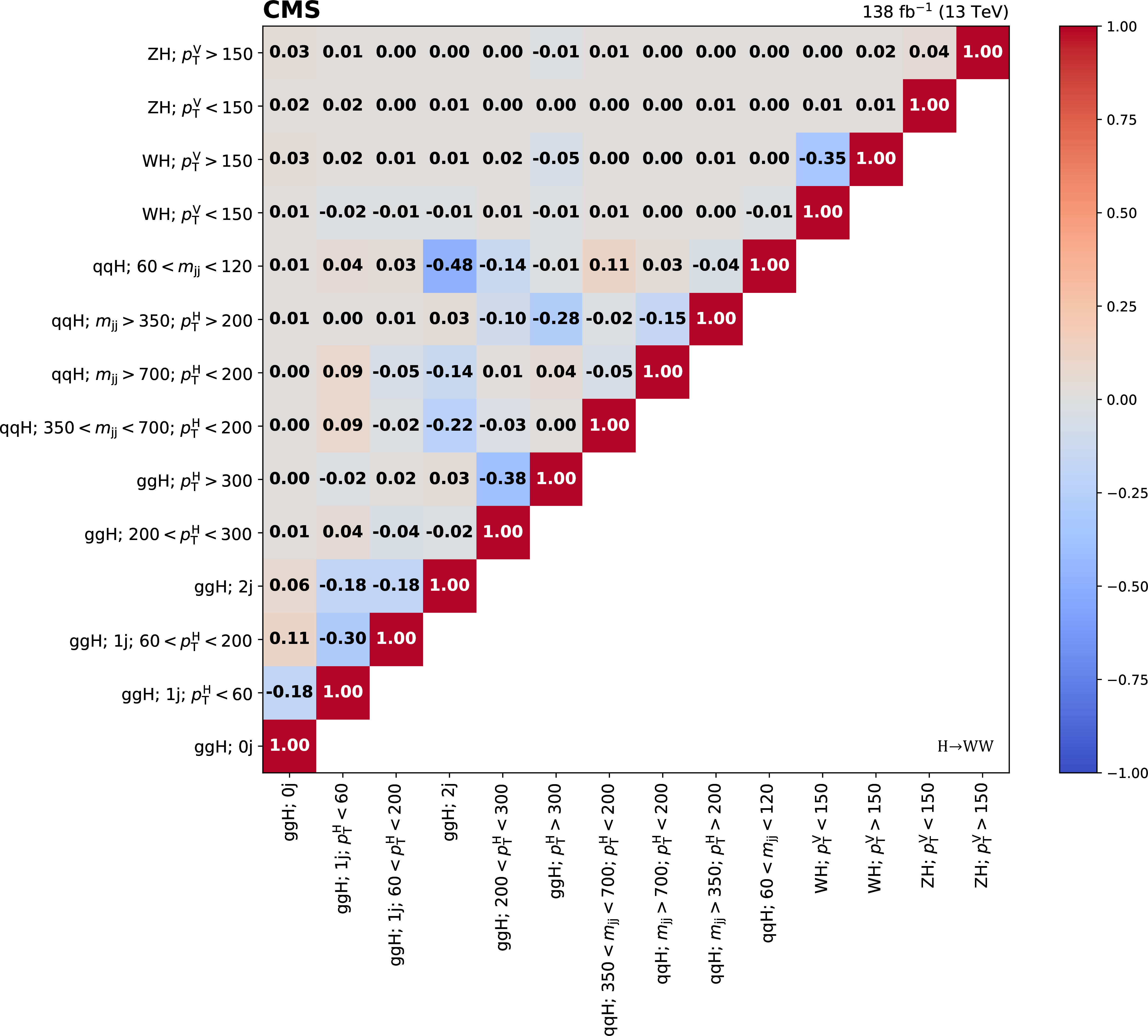
Figure 27:
Correlation matrix between the measured STXS bins. All dimensional quantities in bin definitions are measured in GeV. |
| Tables | |
png pdf |
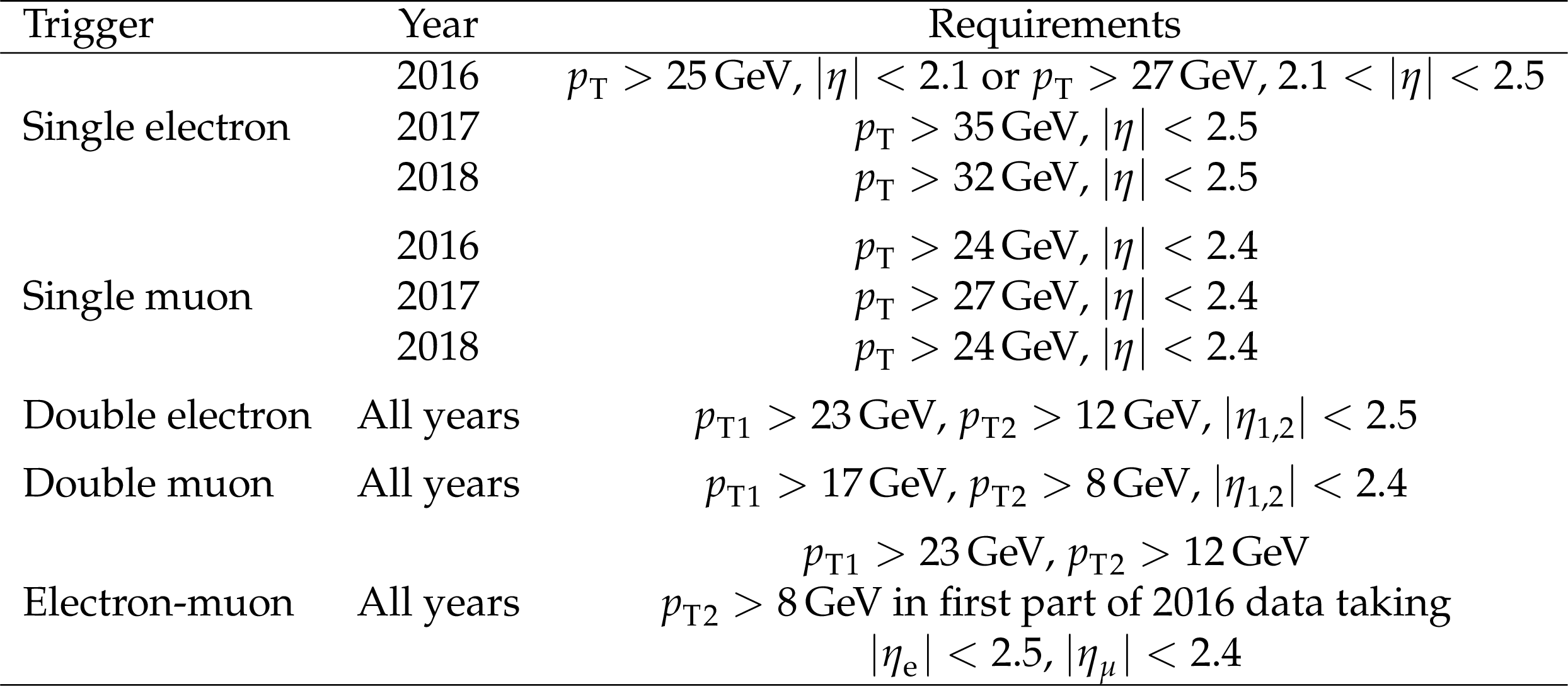
Table 1:
Trigger requirements on the data set used in the analysis. |

png pdf |
Table 2:
Overview of the selection defining the analysis categories (a more detailed breakdown is given in Table 12). |

png pdf |
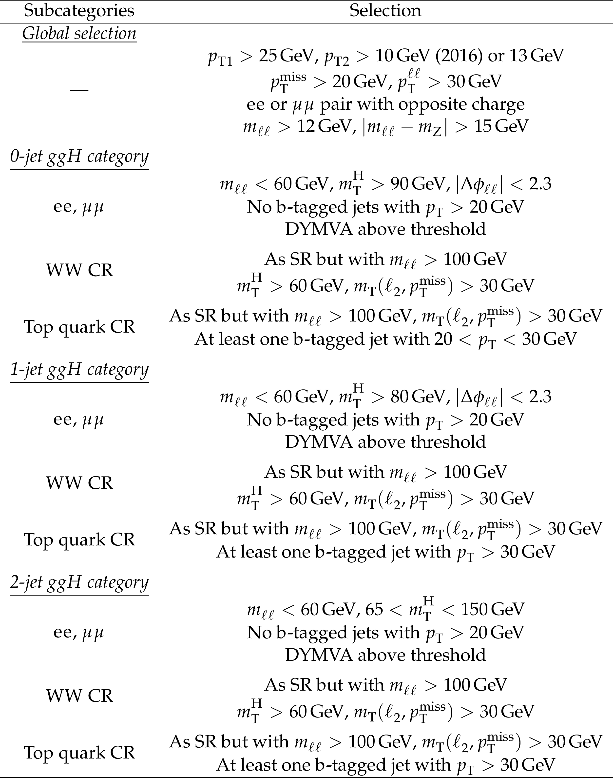
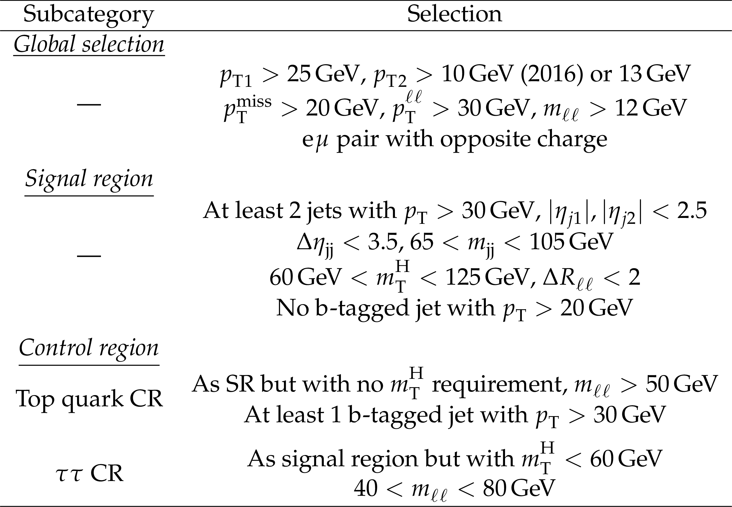
Table 3:
Summary of the selection used in different-flavor ggH categories. |
png pdf |
Table 4:
Summary of the selection used in same-flavor ggH categories. The DYMVA threshold is optimized separately in each subcategory and data set. |
png pdf |
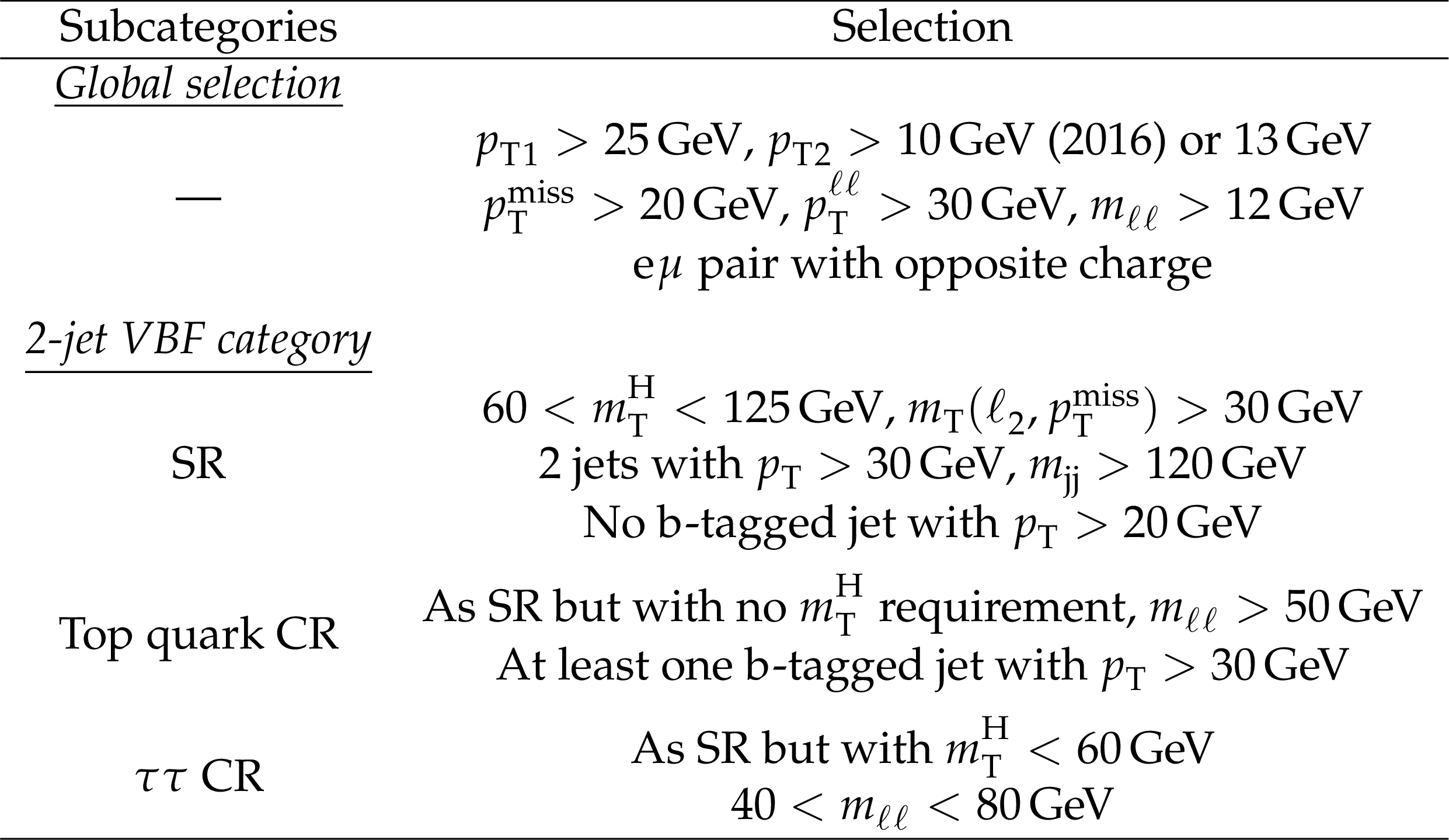
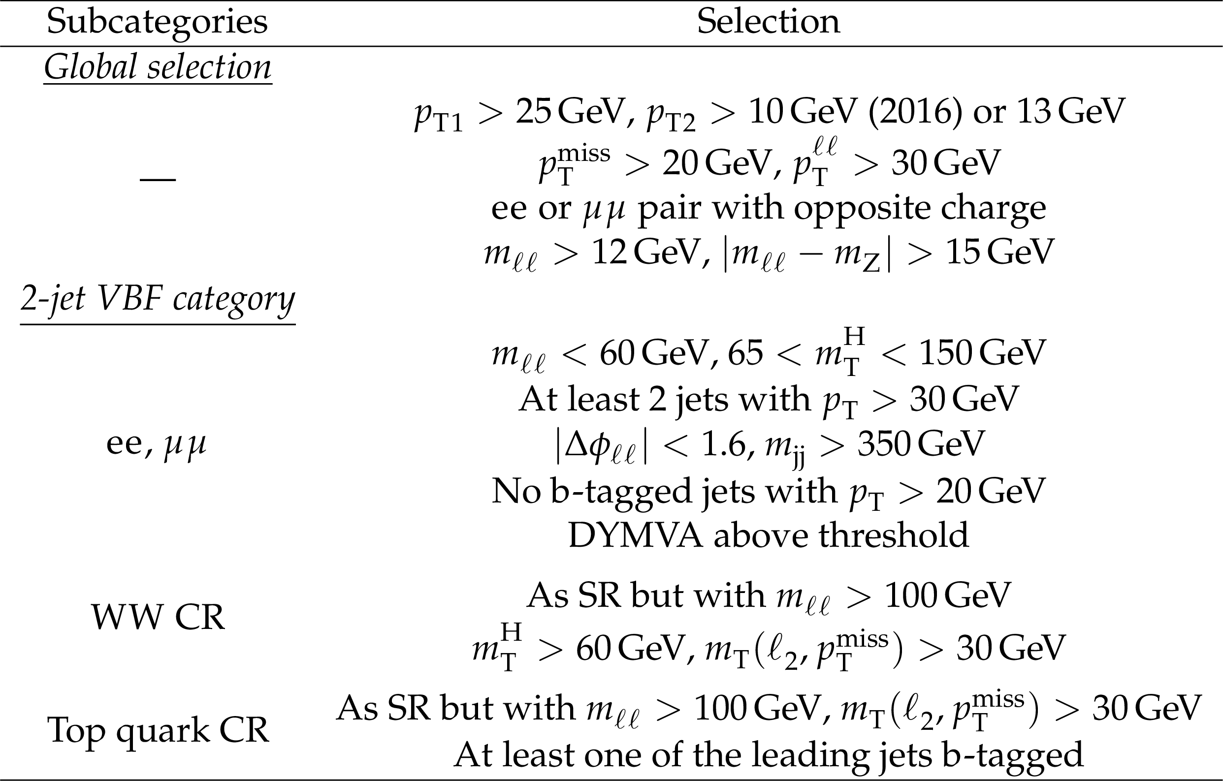
Table 5:
Selection used in the different-flavor VBF categories. |
png pdf |
Table 6:
Selection used in the same-flavor VBF categories. The DYMVA threshold is optimized separately in each subcategory and data set. |
png pdf |
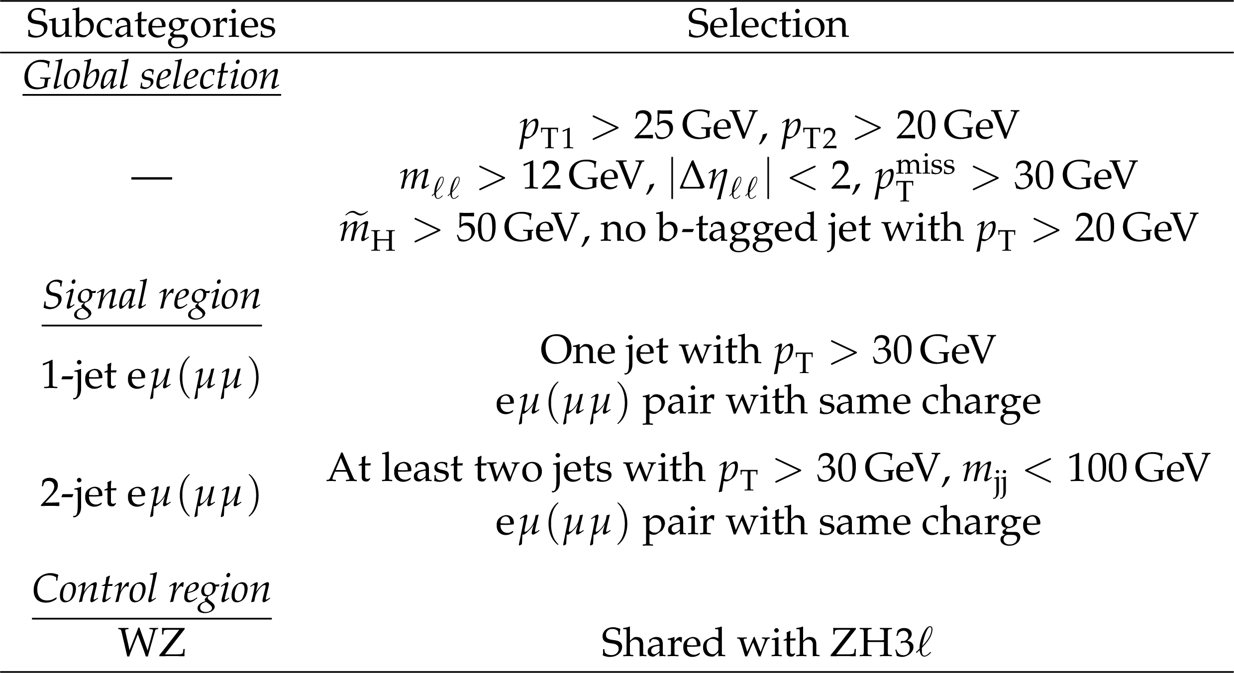
Table 7:
Event selection and categorization in the WHSS category. |
png pdf |
Table 8:
Event selection and categorization in the WH3$\ell$ category. |
png pdf |
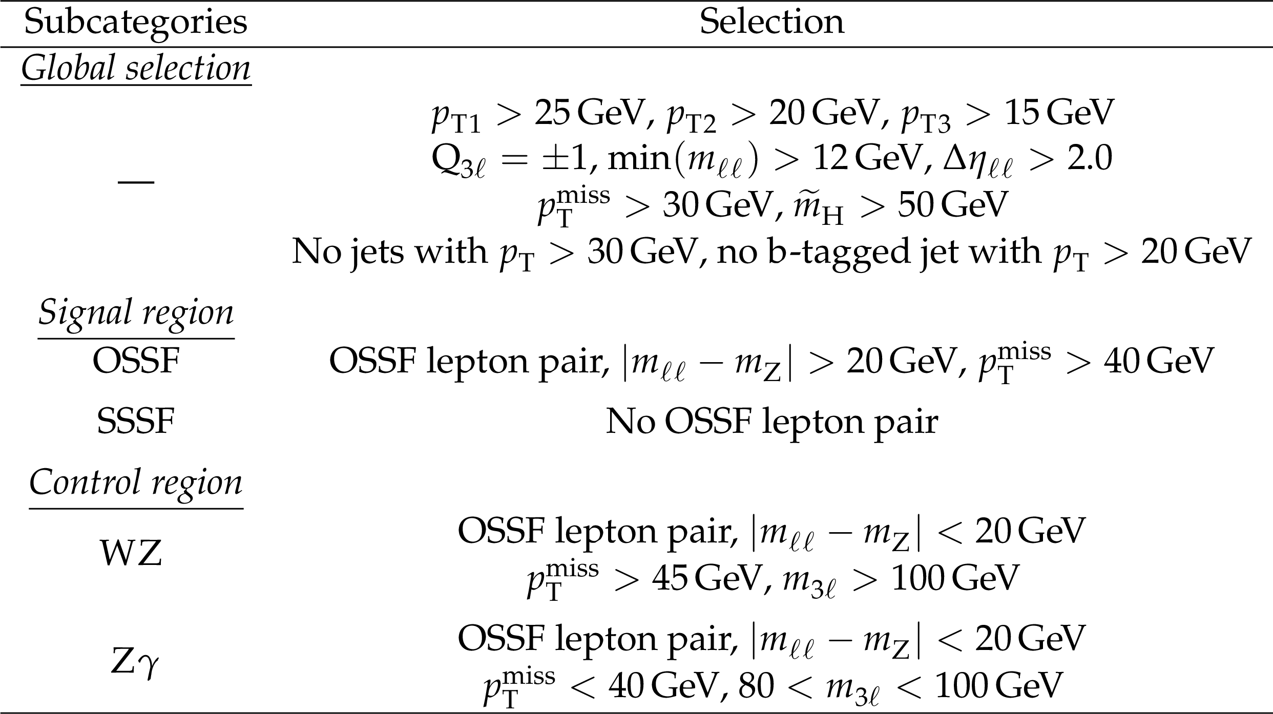
Table 9:
Event selection and categorization in the ZH3$\ell$ category. |
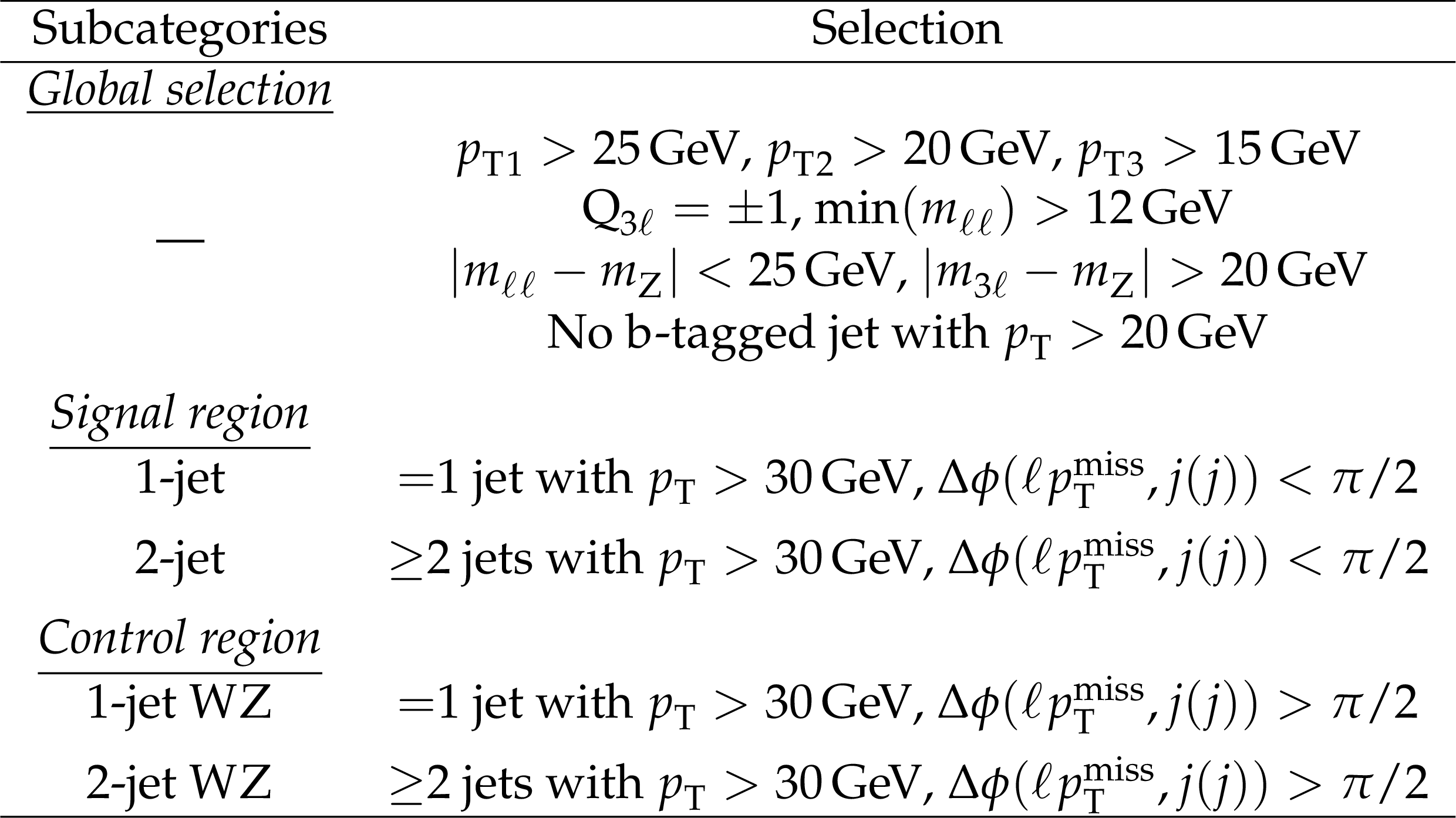
png pdf |
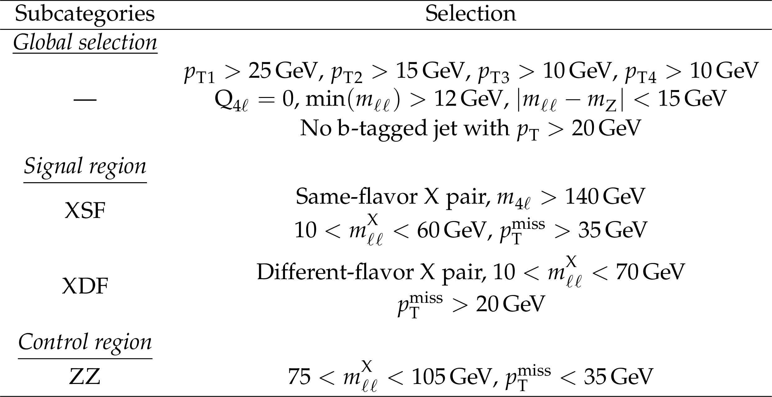
Table 10:
Event selection and categorization in the ZH4$\ell$ category. |
png pdf |
Table 11:
Summary of the selection applied to different-flavor VH2j categories. |
png pdf |
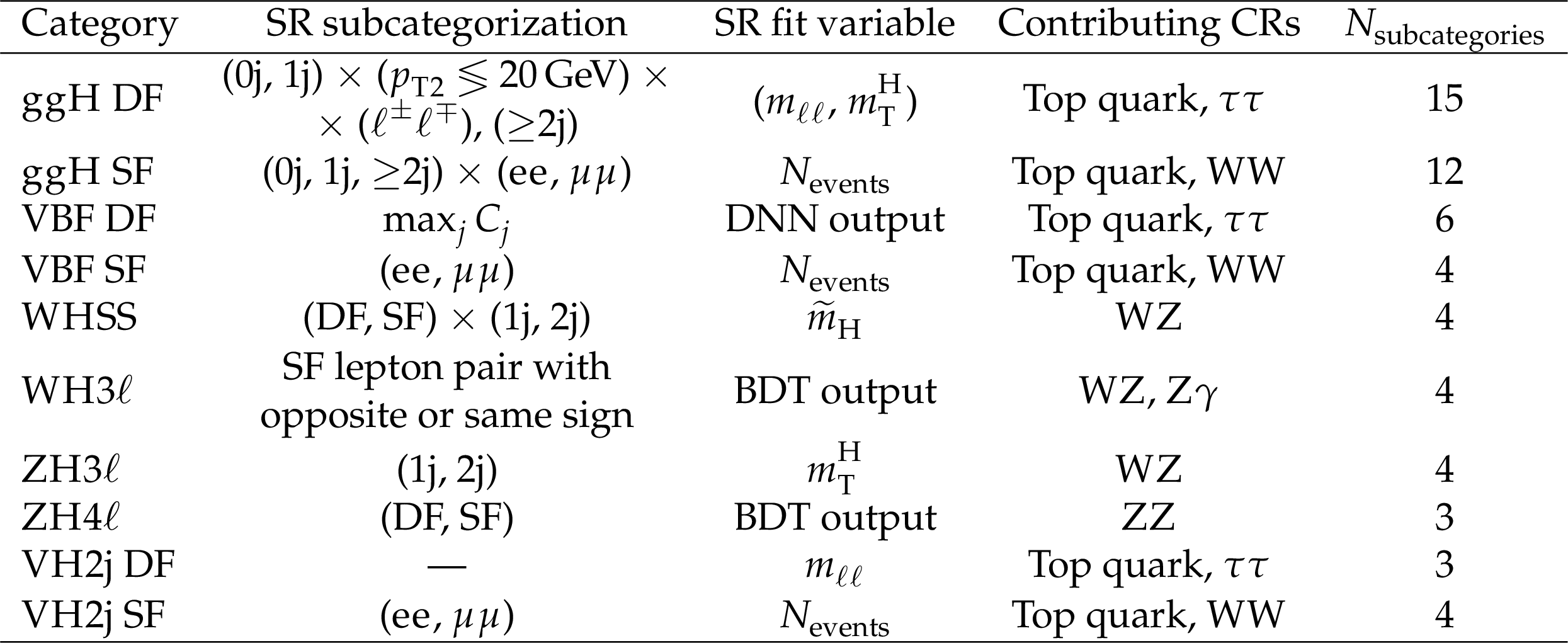
Table 12:
Overview of the fit variables and CRs used in each analysis category. In all CRs, the number of events is used. |

png pdf |
Table 13:
Contributions of different sources of uncertainty in the signal strength measurement. The systematic component includes the combined effect from all sources besides background normalization and the size of the dataset, which make up the statistical part. |
png pdf |
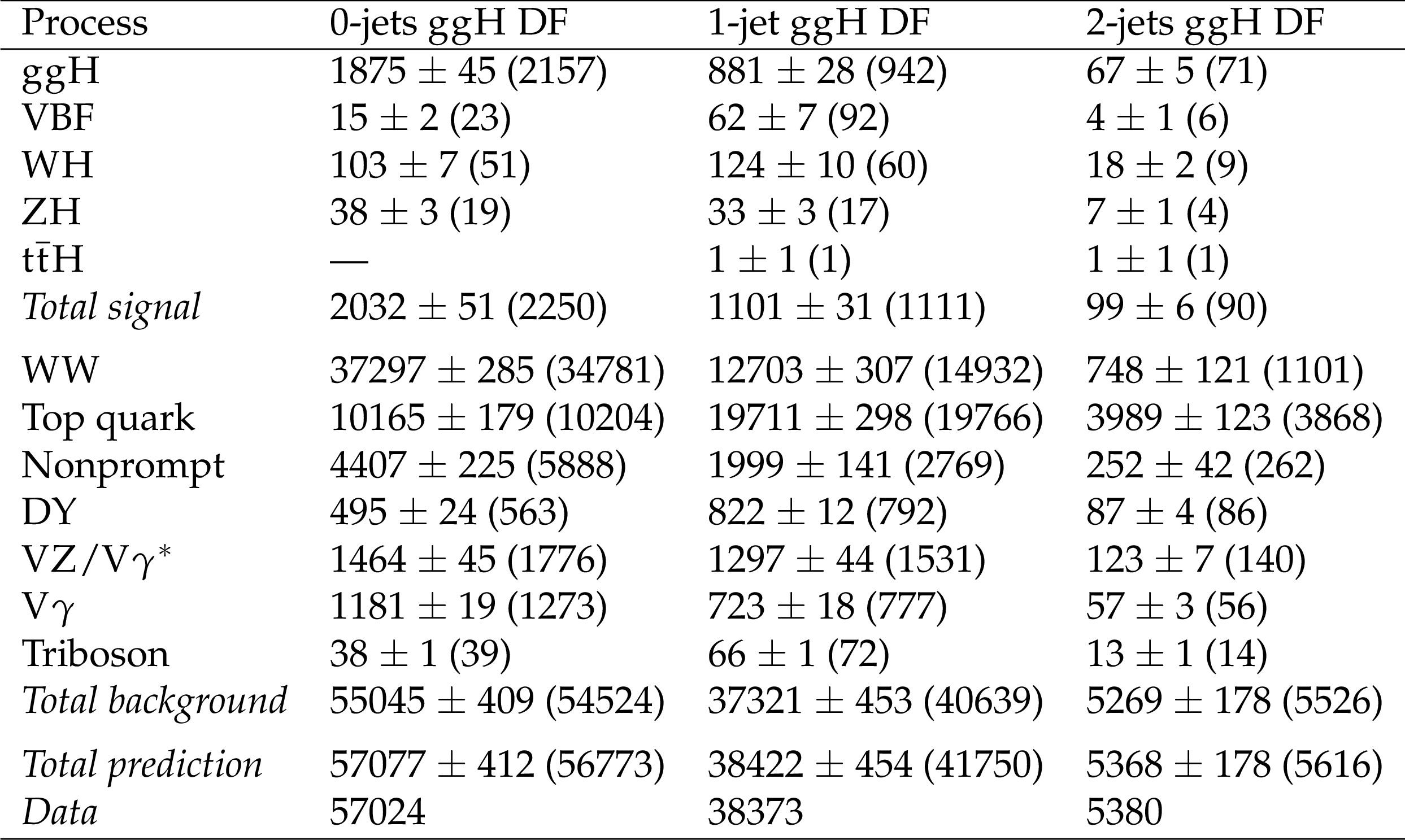
Table 14:
Number of events by process in the ggH DF categories after the fit to the data, scaling the ggH, VBF, WH, and ZH production modes separately. The ${\mathrm{t} {}\mathrm{\bar{t}}}$H contribution is fixed to its SM expectation. Numbers in parenthesis indicate expected yields. |

png pdf |
Table 15:
Number of events by process in the ggH SF categories after the fit to the data, scaling the ggH, VBF, WH, and ZH production modes separately. The ${\mathrm{t} {}\mathrm{\bar{t}}}$H contribution is fixed to its SM expectation. Numbers in parenthesis indicate expected yields. |

png pdf |
Table 16:
Number of events by process in the VBF and VH2j categories after the fit to the data, scaling the ggH, VBF, WH, and ZH production modes separately. The ${\mathrm{t} {}\mathrm{\bar{t}}}$H contribution is fixed to its SM expectation. Numbers in parenthesis indicate expected yields. |

png pdf |
Table 17:
Number of events by process in the ZH4$\ell$, WH3$\ell$, ZH3$\ell$, and ZH4$\ell$ categories after the fit to the data, scaling the ggH, VBF, WH, and ZH production modes separately. The ${\mathrm{t} {}\mathrm{\bar{t}}}$H contribution is fixed to its SM expectation. Numbers in parenthesis indicate expected yields. |
png pdf |
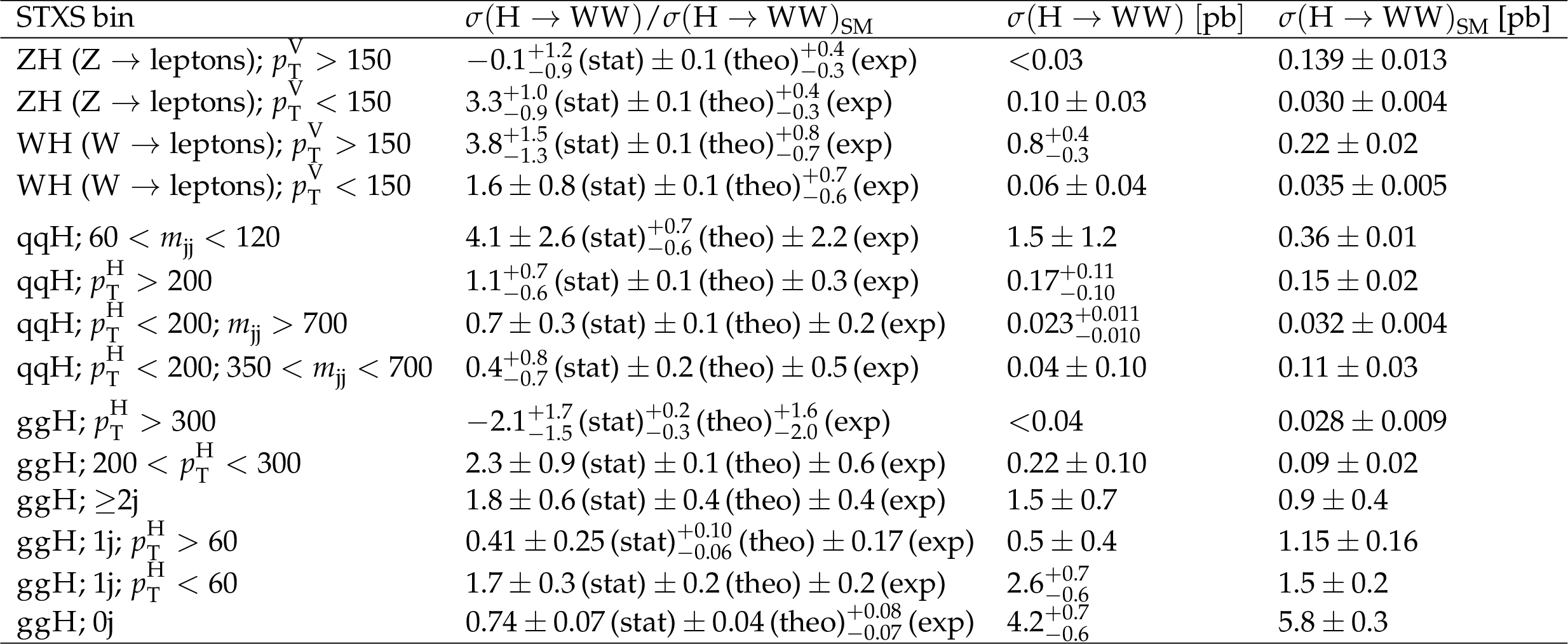
Table 18:
Observed cross sections in each STXS bin. The uncertainties in the observed cross sections and their ratio to the SM expectation do not include the theoretical uncertainties on the latter. In cases where the ratio to the SM cross section is measured below zero, an upper limit at 68% confidence level on the observed cross section is reported. All dimensional quantities in STXS bin definitions are measured in GeV. |
| Summary |
| A measurement of production cross sections for the Higgs boson has been performed targeting the gluon fusion, vector boson fusion, and Z or W associated production processes in the ${\mathrm{H}\to\mathrm{W}\mathrm{W}}$ decay channel. Results are presented as signal strength modifiers, coupling modifiers, and differential cross sections in the simplified template cross section Stage 1.2 framework. The measurement has been performed on data from proton-proton collisions recorded by the CMS detector at a center-of-mass energy of 13 TeV in 2016-2018, corresponding to an integrated luminosity of 138 fb$^{-1}$. Specific event selections targeting different final states have been employed, and results have been extracted via a simultaneous maximum likelihood fit to all analysis categories. The overall signal strength for production of a Higgs boson is found to be $\mu = $ 0.95$^{+0.10}_{-0.09}$. All results are in good agreement with the standard model expectation. |
| References | ||||
| 1 | ATLAS Collaboration | Observation of a new particle in the search for the standard model Higgs boson with the ATLAS detector at the LHC | PLB 716 (2012) 1 | 1207.7214 |
| 2 | CMS Collaboration | Observation of a new boson at a mass of 125 GeV with the CMS experiment at the LHC | PLB 716 (2012) 30 | CMS-HIG-12-028 1207.7235 |
| 3 | CMS Collaboration | Observation of a new boson with mass near 125 GeV in pp collisions at $ \sqrt{s}= $ 7 and 8 TeV | JHEP 06 (2013) 081 | CMS-HIG-12-036 1303.4571 |
| 4 | ATLAS and CMS Collaborations | Measurements of the Higgs boson production and decay rates and constraints on its couplings from a combined ATLAS and CMS analysis of the LHC pp collision data at $ \sqrt{s} = $ 7 and 8 TeV | JHEP 08 (2016) 45 | 1606.02266 |
| 5 | N. Berger et al. | Simplified template cross sections --- stage 1.1 | 2019 | 1906.02754 |
| 6 | CMS Collaboration | Measurement of Higgs boson production and properties in the WW decay channel with leptonic final states | JHEP 01 (2014) 096 | CMS-HIG-13-023 1312.1129 |
| 7 | CMS Collaboration | Measurements of properties of the Higgs boson decaying to a W boson pair in pp collisions at $ \sqrt{s} = $ 13 TeV | PLB 791 (2019) 96 | CMS-HIG-16-042 1806.05246 |
| 8 | CMS Collaboration | Measurement of the transverse momentum spectrum of the Higgs boson produced in pp collisions at $ \sqrt{s} = $ 8 TeV using $ \mathrm{H} \to \mathrm{W}{}\mathrm{W} $ decays | JHEP 03 (2017) 032 | CMS-HIG-15-010 1606.01522 |
| 9 | CMS Collaboration | Measurement of the inclusive and differential Higgs boson production cross sections in the leptonic WW decay mode at $ \sqrt{s} = $ 13 TeV | JHEP 03 (2021) 003 | CMS-HIG-19-002 2007.01984 |
| 10 | CMS Collaboration | Measurement of the inclusive and differential Higgs boson production cross sections in the decay mode to a pair of $ \tau $ leptons in pp collisions at $ \sqrt{s} = $ 13 TeV | PRL 128 (2021) 081805 | CMS-HIG-20-015 2107.11486 |
| 11 | CMS Collaboration | Measurements of Higgs boson production cross sections and couplings in the diphoton decay channel at $ \sqrt{\mathrm{s}} = $ 13 TeV | JHEP 07 (2021) 027 | CMS-HIG-19-015 2103.06956 |
| 12 | CMS Collaboration | Measurements of production cross sections of the Higgs boson in the four-lepton final state in proton-proton collisions at $ \sqrt{s} = $ 13 TeV | EPJC 81 (2021) 488 | CMS-HIG-19-001 2103.04956 |
| 13 | ATLAS Collaboration | Measurements of the Higgs boson inclusive and differential fiducial cross sections in the 4$ \ell $ decay channel at $ \sqrt{s} = $ 13 TeV | EPJC 80 (2020) 942 | 2004.03969 |
| 14 | ATLAS Collaboration | Higgs boson production cross-section measurements and their EFT interpretation in the 4$ \ell $ decay channel at $ \sqrt{s}= $ 13 TeV with the ATLAS detector | EPJC 80 (2020) 957 | 2004.03447 |
| 15 | CMS Collaboration | HEPData record for this analysis | link | |
| 16 | CMS Collaboration | Performance of the CMS Level-1 trigger in proton-proton collisions at $ \sqrt{s} = $ 13 TeV | JINST 15 (2020) P10017 | CMS-TRG-17-001 2006.10165 |
| 17 | CMS Collaboration | The CMS trigger system | JINST 12 (2017) P01020 | CMS-TRG-12-001 1609.02366 |
| 18 | CMS Collaboration | The CMS experiment at the CERN LHC | JINST 3 (2008) S08004 | CMS-00-001 |
| 19 | CMS Collaboration | Performance of the CMS muon detector and muon reconstruction with proton-proton collisions at $ \sqrt{s} = $ 13 TeV | JINST 13 (2018) P06015 | CMS-MUO-16-001 1804.04528 |
| 20 | CMS Collaboration | Performance of the reconstruction and identification of high-momentum muons in proton-proton collisions at $ \sqrt{s} = $ 13 TeV | JINST 15 (2020) P02027 | CMS-MUO-17-001 1912.03516 |
| 21 | CMS Collaboration | Performance of electron reconstruction and selection with the CMS detector in proton-proton collisions at $ \sqrt{s} = $ 8 TeV | JINST 10 (2015) P06005 | CMS-EGM-13-001 1502.02701 |
| 22 | CMS Collaboration | Measurement of the Higgs boson production rate in association with top quarks in final states with electrons, muons, and hadronically decaying tau leptons at $ \sqrt{s} = $ 13 TeV | EPJC 81 (2021) 378 | CMS-HIG-19-008 2011.03652 |
| 23 | W. Waltenberger, R. Fruhwirth, and P. Vanlaer | Adaptive vertex fitting | JPG 34 (2007) N343 | |
| 24 | CMS Collaboration | Technical proposal for the Phase-II upgrade of the Compact Muon Solenoid | CMS-PAS-TDR-15-002 | CMS-PAS-TDR-15-002 |
| 25 | CMS Collaboration | Particle-flow reconstruction and global event description with the CMS detector | JINST 12 (2017) P10003 | CMS-PRF-14-001 1706.04965 |
| 26 | M. Cacciari, G. P. Salam, and G. Soyez | The anti-$ {k_{\mathrm{T}}} $ jet clustering algorithm | JHEP 04 (2008) 063 | 0802.1189 |
| 27 | M. Cacciari, G. P. Salam, and G. Soyez | FastJet user manual | EPJC 72 (2012) 1896 | 1111.6097 |
| 28 | CMS Collaboration | Jet energy scale and resolution in the CMS experiment in pp collisions at 8 TeV | JINST 12 (2017) P02014 | CMS-JME-13-004 1607.03663 |
| 29 | CMS Collaboration | Jet energy scale and resolution performance with 13 TeV data collected by CMS in 2016-2018 | CDS | |
| 30 | CMS Collaboration | Jet algorithms performance in 13 TeV data | CMS-PAS-JME-16-003 | CMS-PAS-JME-16-003 |
| 31 | CMS Collaboration | Identification of heavy-flavour jets with the CMS detector in pp collisions at 13 TeV | JINST 13 (2018) P05011 | CMS-BTV-16-002 1712.07158 |
| 32 | CMS Collaboration | CMS Phase 1 heavy flavour identification performance and developments | CDS | |
| 33 | CMS Collaboration | Performance of missing transverse momentum reconstruction in proton-proton collisions at $ \sqrt{s} = $ 13 TeV using the CMS detector | JINST 14 (2019) P07004 | CMS-JME-17-001 1903.06078 |
| 34 | D. Bertolini, P. Harris, M. Low, and N. Tran | Pileup per particle identification | JHEP 10 (2014) 059 | 1407.6013 |
| 35 | CMS Collaboration | Precision luminosity measurement in proton-proton collisions at $ \sqrt{s} = $ 13 TeV in 2015 and 2016 at CMS | EPJC 81 (2021) 800 | CMS-LUM-17-003 2104.01927 |
| 36 | CMS Collaboration | CMS luminosity measurement for the 2017 data-taking period at $ \sqrt{s} = $ 13 TeV | CMS-PAS-LUM-17-004 | CMS-PAS-LUM-17-004 |
| 37 | CMS Collaboration | CMS luminosity measurement for the 2018 data-taking period at $ \sqrt{s} = $ 13 TeV | CMS-PAS-LUM-18-002 | CMS-PAS-LUM-18-002 |
| 38 | NNPDF Collaboration | Parton distributions with QED corrections | NPB 877 (2013) 290 | 1308.0598 |
| 39 | NNPDF Collaboration | Unbiased global determination of parton distributions and their uncertainties at NNLO and at LO | NPB 855 (2012) 153 | 1107.2652 |
| 40 | NNPDF Collaboration | Parton distributions from high-precision collider data | EPJC 77 (2017) 663 | 1706.00428 |
| 41 | CMS Collaboration | Event generator tunes obtained from underlying event and multiparton scattering measurements | EPJC 76 (2016) 155 | CMS-GEN-14-001 1512.00815 |
| 42 | CMS Collaboration | Extraction and validation of a new set of CMS PYTHIA-8 tunes from underlying-event measurements | EPJC 80 (2020) 4 | CMS-GEN-17-001 1903.12179 |
| 43 | T. Sjostrand et al. | An introduction to PYTHIA 8.2 | CPC 191 (2015) 159 | 1410.3012 |
| 44 | P. Nason | A new method for combining NLO QCD with shower Monte Carlo algorithms | JHEP 11 (2004) 040 | hep-ph/0409146 |
| 45 | S. Frixione, P. Nason, and C. Oleari | Matching NLO QCD computations with parton shower simulations: the POWHEG method | JHEP 11 (2007) 070 | 0709.2092 |
| 46 | S. Alioli, P. Nason, C. Oleari, and E. Re | A general framework for implementing NLO calculations in shower Monte Carlo programs: the POWHEG BOX | JHEP 06 (2010) 043 | 1002.2581 |
| 47 | E. Bagnaschi, G. Degrassi, P. Slavich, and A. Vicini | Higgs production via gluon fusion in the POWHEG approach in the SM and in the MSSM | JHEP 02 (2012) 088 | 1111.2854 |
| 48 | P. Nason and C. Oleari | NLO Higgs boson production via vector-boson fusion matched with shower in POWHEG | JHEP 02 (2010) 037 | 0911.5299 |
| 49 | G. Luisoni, P. Nason, C. Oleari, and F. Tramontano | HW$^{\pm} $/HZ + 0 and 1 jet at NLO with the POWHEG BOX interfaced to GoSam and their merging within MiNLO | JHEP 10 (2013) 083 | 1306.2542 |
| 50 | H. B. Hartanto, B. Jager, L. Reina, and D. Wackeroth | Higgs boson production in association with top quarks in the POWHEG BOX | PRD 91 (2015) 094003 | 1501.04498 |
| 51 | J. Alwall et al. | The automated computation of tree-level and next-to-leading order differential cross sections, and their matching to parton shower simulations | JHEP 07 (2014) 079 | 1405.0301 |
| 52 | K. Hamilton, P. Nason, E. Re, and G. Zanderighi | NNLOPS simulation of Higgs boson production | JHEP 10 (2013) 222 | 1309.0017 |
| 53 | K. Hamilton, P. Nason, and G. Zanderighi | Finite quark-mass effects in the NNLOPS POWHEG+MiNLO Higgs generator | JHEP 05 (2015) 140 | 1501.04637 |
| 54 | R. Frederix and K. Hamilton | Extending the MINLO method | JHEP 05 (2016) 042 | 1512.02663 |
| 55 | LHC Higgs Cross Section Working Group | Handbook of LHC Higgs cross sections: 4. Deciphering the nature of the Higgs sector | CERN-2017-002-M | 1610.07922 |
| 56 | CMS Collaboration | A measurement of the Higgs boson mass in the diphoton decay channel | PLB 805 (2020) 135425 | CMS-HIG-19-004 2002.06398 |
| 57 | S. Bolognesi et al. | On the spin and parity of a single-produced resonance at the LHC | PRD 86 (2012) 095031 | 1208.4018 |
| 58 | P. Nason and G. Zanderighi | W$^+ $W$^- $, WZ and ZZ production in the POWHEG-BOX-V2 | EPJC 74 (2014) 2702 | 1311.1365 |
| 59 | J. M. Campbell and R. K. Ellis | An update on vector boson pair production at hadron colliders | PRD 60 (1999) 113006 | hep-ph/9905386 |
| 60 | J. M. Campbell, R. K. Ellis, and C. Williams | Vector boson pair production at the LHC | JHEP 07 (2011) 018 | 1105.0020 |
| 61 | J. M. Campbell, R. K. Ellis, and W. T. Giele | A multi-threaded version of MCFM | EPJC 75 (2015) 246 | 1503.06182 |
| 62 | F. Caola et al. | QCD corrections to vector boson pair production in gluon fusion including interference effects with off-shell Higgs at the LHC | JHEP 07 (2016) 087 | 1605.04610 |
| 63 | J. Alwall et al. | Comparative study of various algorithms for the merging of parton showers and matrix elements in hadronic collisions | EPJC 53 (2008) 473 | 0706.2569 |
| 64 | S. Frixione, P. Nason, and G. Ridolfi | A positive-weight next-to-leading-order Monte Carlo for heavy flavour hadroproduction | JHEP 09 (2007) 126 | 0707.3088 |
| 65 | S. Alioli, P. Nason, C. Oleari, and E. Re | NLO single-top production matched with shower in POWHEG: $ s $- and $ t $-channel contributions | JHEP 09 (2009) 111 | 0907.4076 |
| 66 | E. Re | Single-top Wt-channel production matched with parton showers using the POWHEG method | EPJC 71 (2011) 1547 | 1009.2450 |
| 67 | R. Frederix and S. Frixione | Merging meets matching in MC@NLO | JHEP 12 (2012) 061 | 1209.6215 |
| 68 | GEANT4 Collaboration | GEANT4 --- a simulation toolkit | NIMA 506 (2003) 250 | |
| 69 | M. Abadi et al. | TensorFlow: Large-scale machine learning on heterogeneous systems | 2015 Software available from tensorflow.org | |
| 70 | A. Hoecker et al. | TMVA 4 - toolkit for multivariate data analysis with ROOT | 2018 | |
| 71 | CMS Collaboration | Measurements of inclusive W and Z cross sections in pp collisions at $ \sqrt{s}= $ 7 TeV | JHEP 01 (2011) 080 | CMS-EWK-10-002 1012.2466 |
| 72 | M. Czakon et al. | Top-pair production at the LHC through NNLO QCD and NLO EW | JHEP 10 (2017) 186 | 1705.04105 |
| 73 | P. Meade, H. Ramani, and M. Zeng | Transverse momentum resummation effects in $ \mathrm{W}^+{}\mathrm{W}^- $ measurements | PRD 90 (2014) 114006 | 1407.4481 |
| 74 | P. Jaiswal and T. Okui | Explanation of the WW excess at the LHC by jet-veto resummation | PRD 90 (2014) 073009 | 1407.4537 |
| 75 | CMS Collaboration | An embedding technique to determine $ \tau\tau $ backgrounds in proton-proton collision data | JINST 14 (2019) P06032 | CMS-TAU-18-001 1903.01216 |
| 76 | ATLAS and CMS Collaborations, LHC Higgs Combination Group | Procedure for the LHC Higgs boson search combination in Summer 2011 | ATL-PHYS-PUB 2011-11, CMS NOTE 2011/005 | |
| 77 | R. Barlow and C. Beeston | Fitting using finite Monte Carlo samples | CPC 77 (1993) 219 | |
| 78 | ATLAS Collaboration | Measurement of the inelastic proton-proton cross section at $ \sqrt{s} = $ 13 TeV with the ATLAS detector at the LHC | PRL 117 (2016) 182002 | 1606.02625 |
| 79 | CMS Collaboration | Measurement of the inelastic proton-proton cross section at $ \sqrt{s} = $ 13 TeV | JHEP 07 (2018) 161 | CMS-FSQ-15-005 1802.02613 |
| 80 | LHC Higgs Cross Section Working Group | Handbook of LHC Higgs cross sections: 3. Higgs properties: Report of the LHC Higgs Cross Section Working Group | CERN-2013-004 | 1307.1347 |
|
|
Compact Muon Solenoid LHC, CERN |
|

|

|

|

|

|