

Compact Muon Solenoid
LHC, CERN
| CMS-HIG-20-014 ; CERN-EP-2021-094 | ||
| Search for a heavy Higgs boson decaying into two lighter Higgs bosons in the $\tau\tau\mathrm{b}\mathrm{b}$ final state at 13 TeV | ||
| CMS Collaboration | ||
| 18 June 2021 | ||
| JHEP 11 (2021) 057 | ||
| Abstract: A search for a heavy Higgs boson H decaying into the observed Higgs boson H with a mass of 125 GeV and another Higgs boson $\mathrm{h_S}$ is presented. The H and $\mathrm{h_S}$ bosons are required to decay into a pair of tau leptons and a pair of b quarks, respectively. The search uses a sample of proton-proton collisions collected with the CMS detector at a center-of-mass energy of 13 TeV, corresponding to an integrated luminosity of 137 fb$^{-1}$ . Mass ranges of 240-3000 GeV for ${m_{\mathrm{H}}}$ and 60-2800 GeV for ${m_{\mathrm{h_S}}}$ are explored in the search. No signal has been observed. Model independent 95% confidence level upper limits on the product of the production cross section and the branching fractions of the signal process are set with a sensitivity ranging from 125 fb (for ${m_{\mathrm{H}}} = $ 240 GeV) to 2.7 fb (for ${m_{\mathrm{H}}} = $ 1000 GeV). These limits are compared to maximally allowed products of the production cross section and the branching fractions of the signal process in the next-to-minimal supersymmetric extension of the standard model. | ||
| Links: e-print arXiv:2106.10361 [hep-ex] (PDF) ; CDS record ; inSPIRE record ; HepData record ; CADI line (restricted) ; | ||
| Figures & Tables | Summary | Additional Figures & Tables | References | CMS Publications |
|---|
| Figures | |
png pdf |
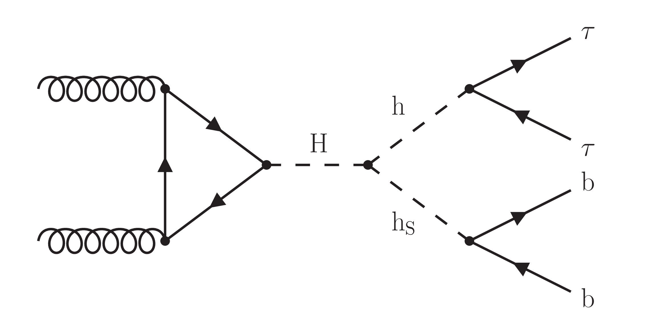
Figure 1:
Feynman diagram of the $\mathrm{g} \mathrm{g} \to \mathrm{H} \to \mathrm{h} (\tau \tau) {\mathrm{h} _{\text {S}}} (\mathrm{b} \mathrm{b})$ process. |
png pdf |
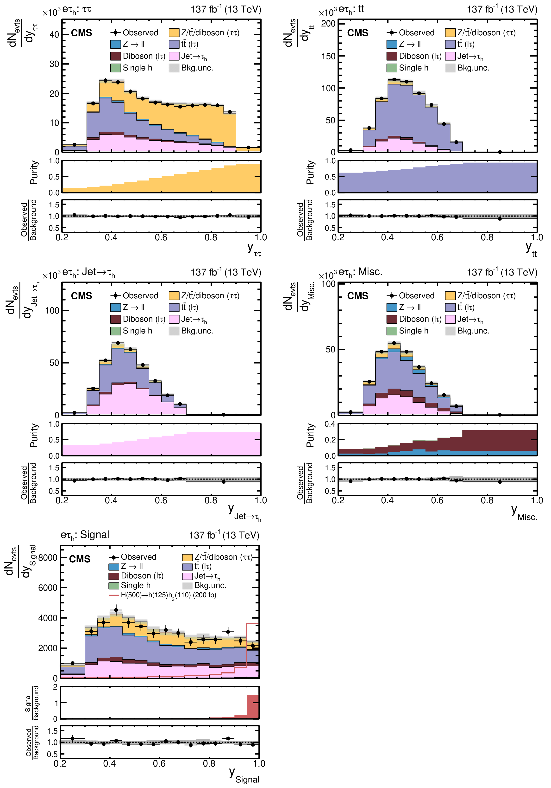
Figure 2:
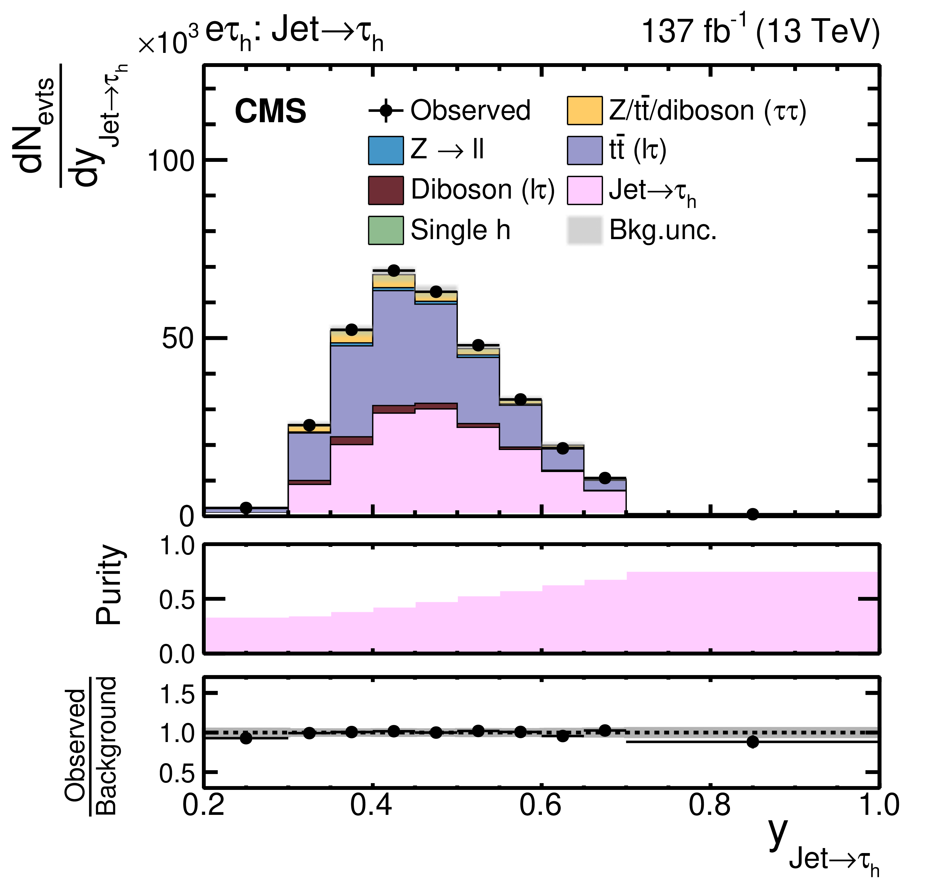
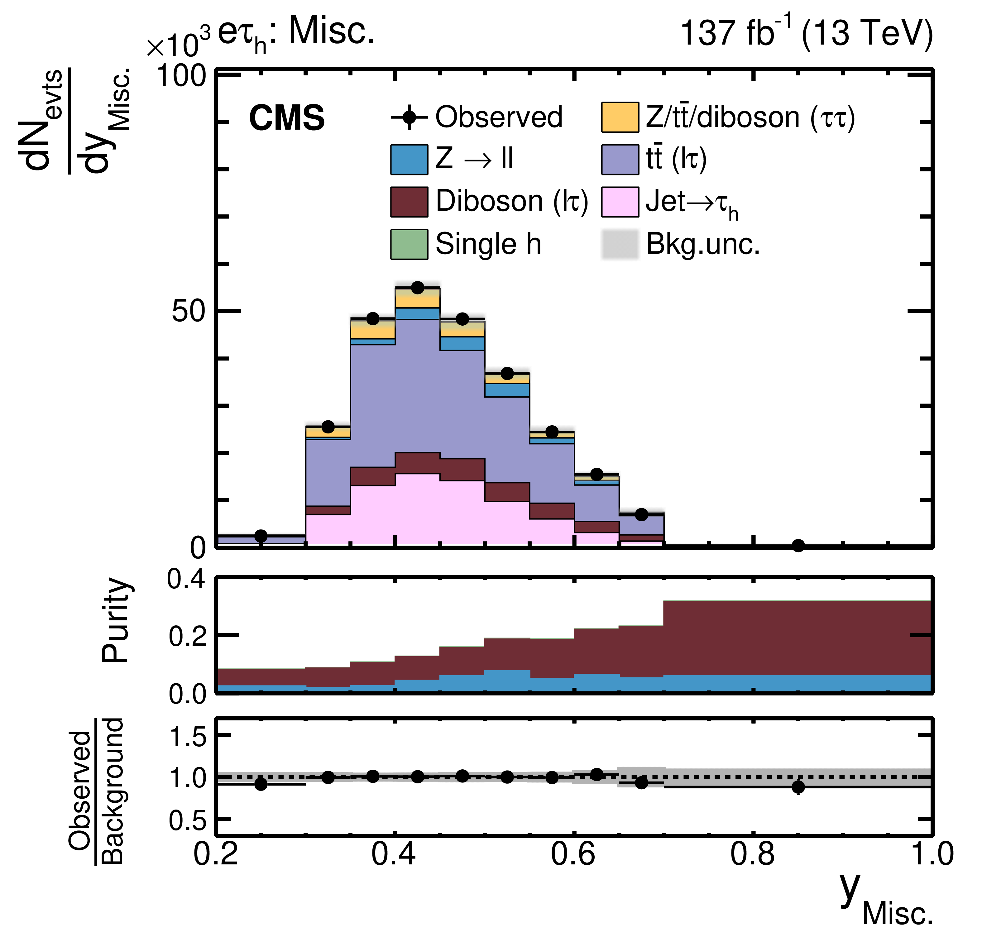
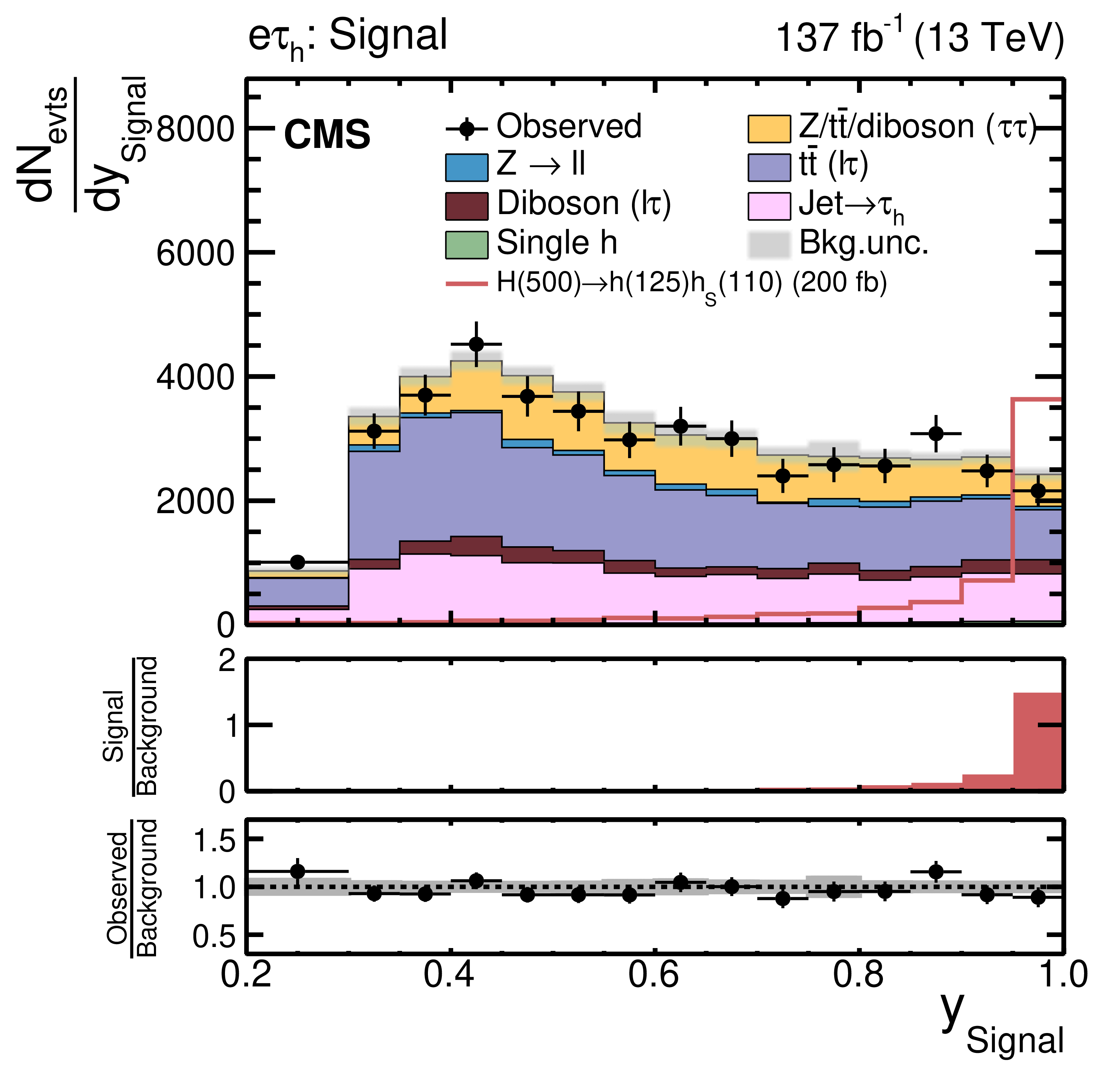
Event categories after NN classification based on a training for $ {m_{\mathrm{H}}} = $ 500 GeV and 100 $\leq {m_{{\mathrm{h} _{\text {S}}}}} < $ 150 GeV in the e$ {\tau _\mathrm {h}} $ final state. Shown are the (upper left) $\tau \tau $, (upper right) tt, (middle left) $ {\text {jet}\to {\tau _\mathrm {h}}}$, (middle right) misc, and (lower left) signal categories. For these figures the data sets of all years have been combined. The uncertainty bands correspond to the combination of statistical and systematic uncertainties after the fit to the signal plus background hypothesis for $ {m_{\mathrm{H}}} = $ 500 GeV and $ {m_{{\mathrm{h} _{\text {S}}}}} = $ 110 GeV. |
png pdf |
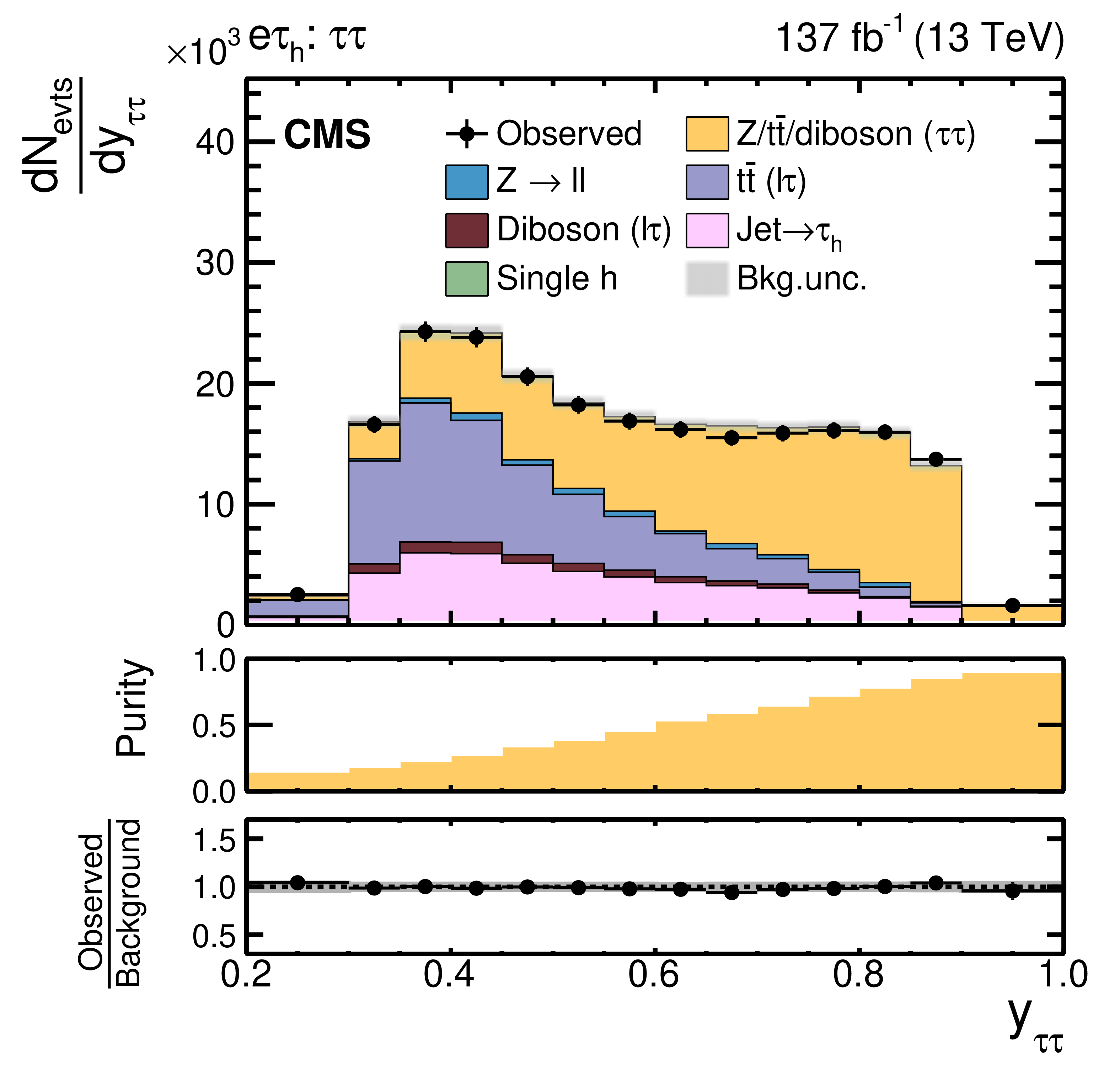
Figure 2-a:
Shown is the $\tau \tau $ category, obtained by NN classification based on a training for $ {m_{\mathrm{H}}} = $ 500 GeV and 100 $\leq {m_{{\mathrm{h} _{\text {S}}}}} < $ 150 GeV in the e$ {\tau _\mathrm {h}} $ final state. The data sets of all years have been combined. The uncertainty bands correspond to the combination of statistical and systematic uncertainties after the fit to the signal plus background hypothesis for $ {m_{\mathrm{H}}} = $ 500 GeV and $ {m_{{\mathrm{h} _{\text {S}}}}} = $ 110 GeV. |
png pdf |
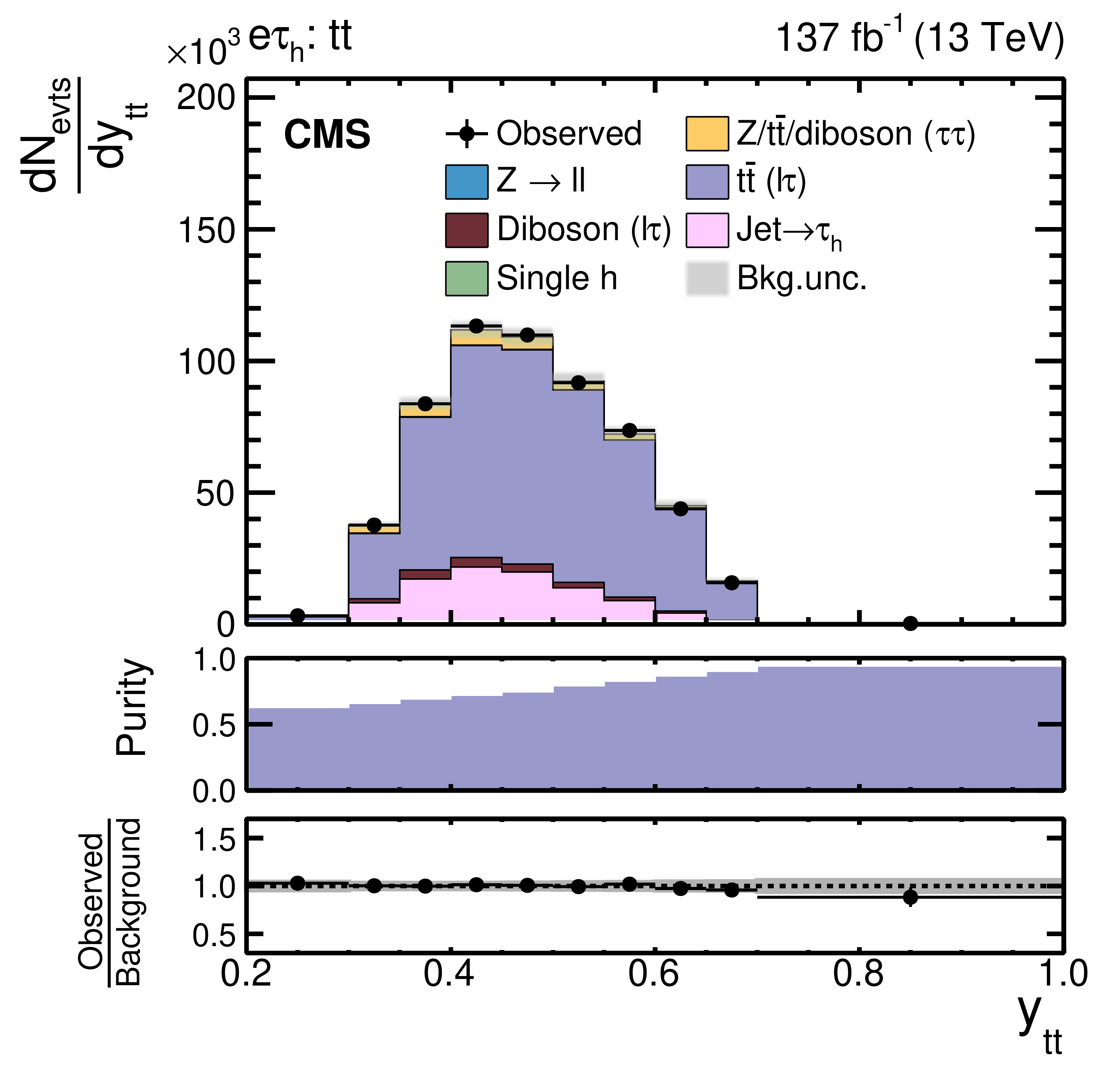
Figure 2-b:
Shown is the tt category, obtained by NN classification based on a training for $ {m_{\mathrm{H}}} = $ 500 GeV and 100 $\leq {m_{{\mathrm{h} _{\text {S}}}}} < $ 150 GeV in the e$ {\tau _\mathrm {h}} $ final state. The data sets of all years have been combined. The uncertainty bands correspond to the combination of statistical and systematic uncertainties after the fit to the signal plus background hypothesis for $ {m_{\mathrm{H}}} = $ 500 GeV and $ {m_{{\mathrm{h} _{\text {S}}}}} = $ 110 GeV. |
png pdf |
Figure 2-c:
Shown is the $ {\text {jet}\to {\tau _\mathrm {h}}}$ category, obtained by NN classification based on a training for $ {m_{\mathrm{H}}} = $ 500 GeV and 100 $\leq {m_{{\mathrm{h} _{\text {S}}}}} < $ 150 GeV in the e$ {\tau _\mathrm {h}} $ final state. The data sets of all years have been combined. The uncertainty bands correspond to the combination of statistical and systematic uncertainties after the fit to the signal plus background hypothesis for $ {m_{\mathrm{H}}} = $ 500 GeV and $ {m_{{\mathrm{h} _{\text {S}}}}} = $ 110 GeV. |
png pdf |
Figure 2-d:
Shown is the misc signal category, obtained by NN classification based on a training for $ {m_{\mathrm{H}}} = $ 500 GeV and 100 $\leq {m_{{\mathrm{h} _{\text {S}}}}} < $ 150 GeV in the e$ {\tau _\mathrm {h}} $ final state. The data sets of all years have been combined. The uncertainty bands correspond to the combination of statistical and systematic uncertainties after the fit to the signal plus background hypothesis for $ {m_{\mathrm{H}}} = $ 500 GeV and $ {m_{{\mathrm{h} _{\text {S}}}}} = $ 110 GeV. |
png pdf |
Figure 2-e:
Shown is the signal category, obtained by NN classification based on a training for $ {m_{\mathrm{H}}} = $ 500 GeV and 100 $\leq {m_{{\mathrm{h} _{\text {S}}}}} < $ 150 GeV in the e$ {\tau _\mathrm {h}} $ final state. The data sets of all years have been combined. The uncertainty bands correspond to the combination of statistical and systematic uncertainties after the fit to the signal plus background hypothesis for $ {m_{\mathrm{H}}} = $ 500 GeV and $ {m_{{\mathrm{h} _{\text {S}}}}} = $ 110 GeV. |
png pdf |
Figure 3:
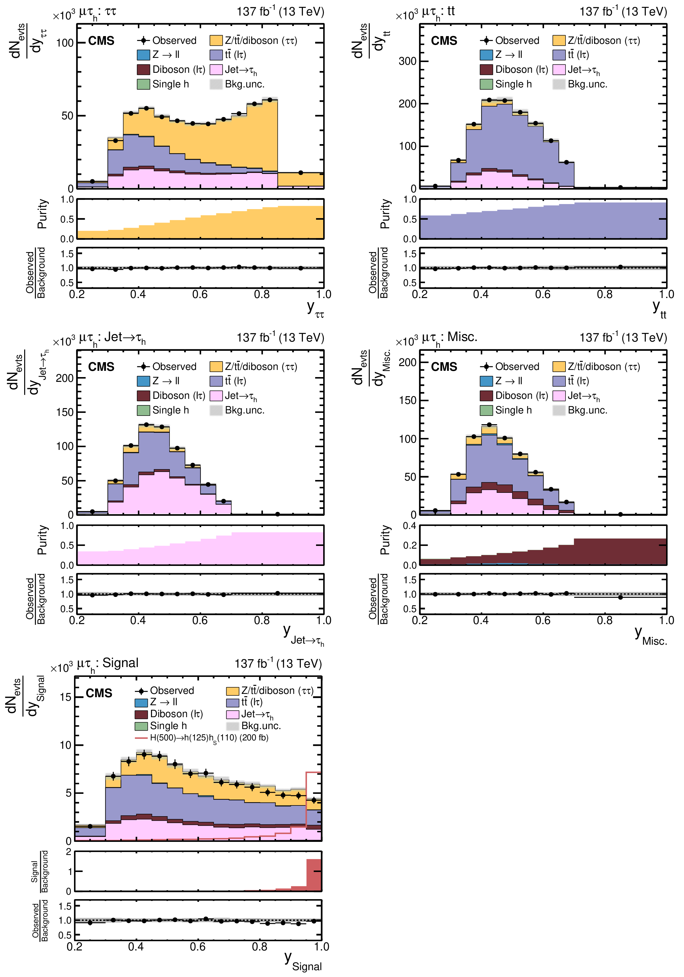
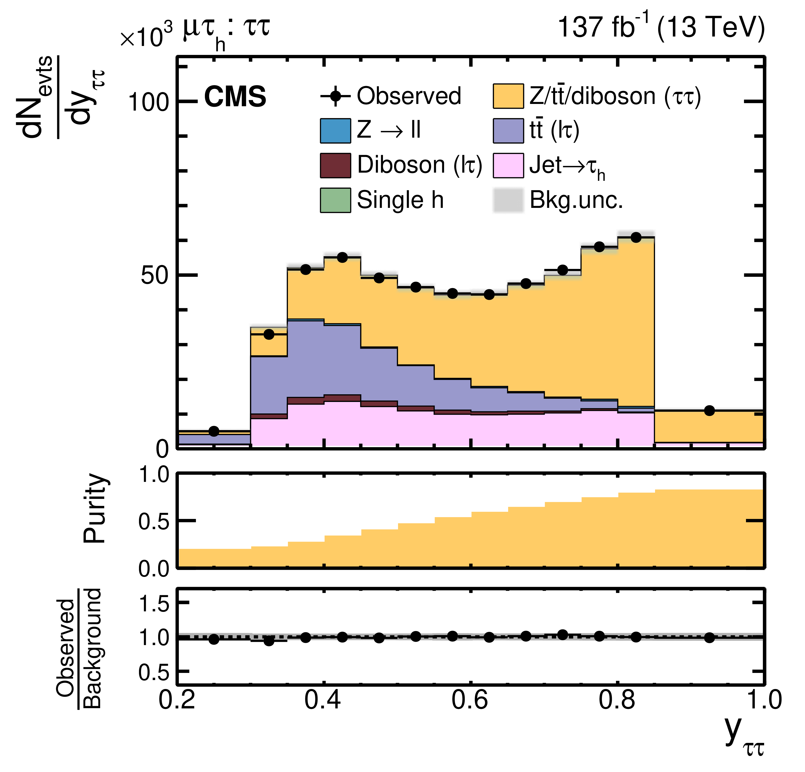
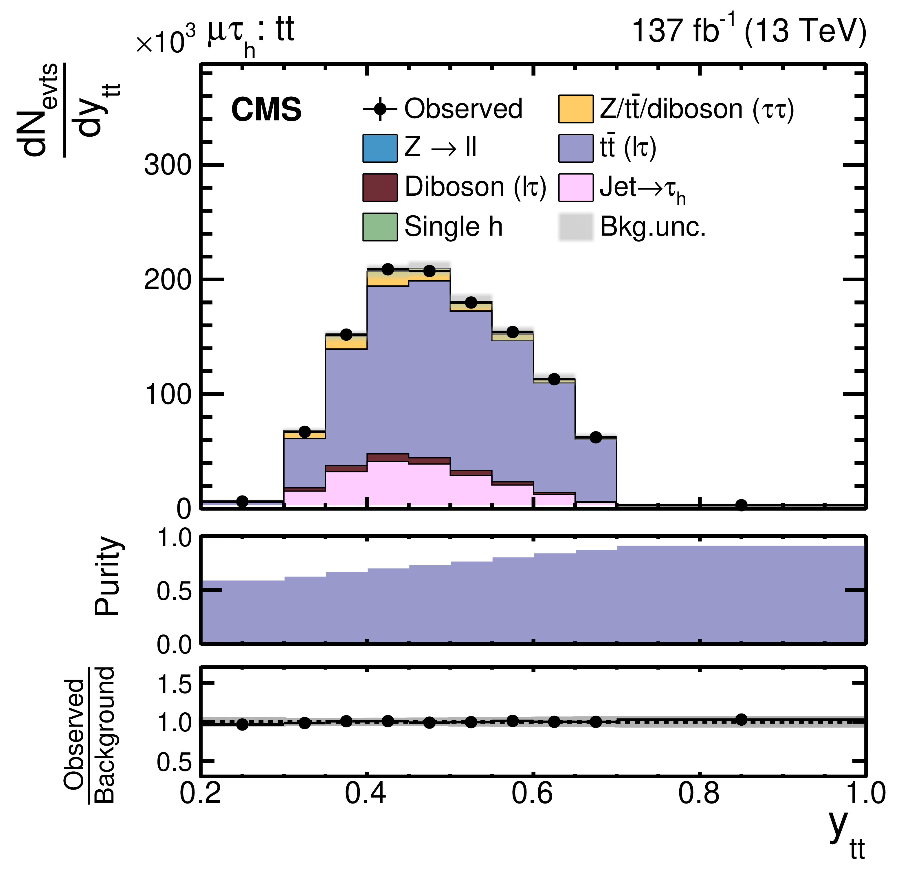
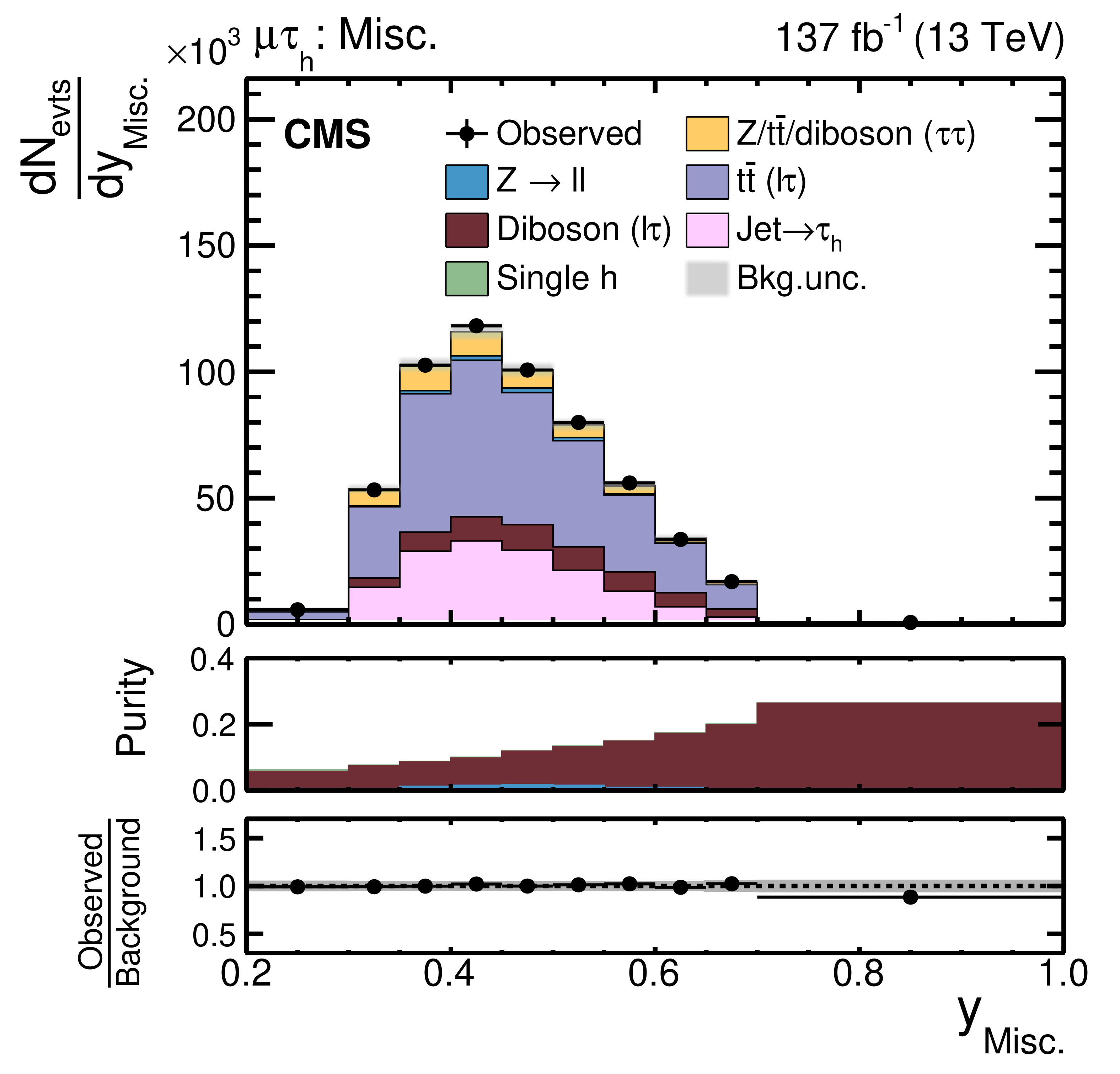
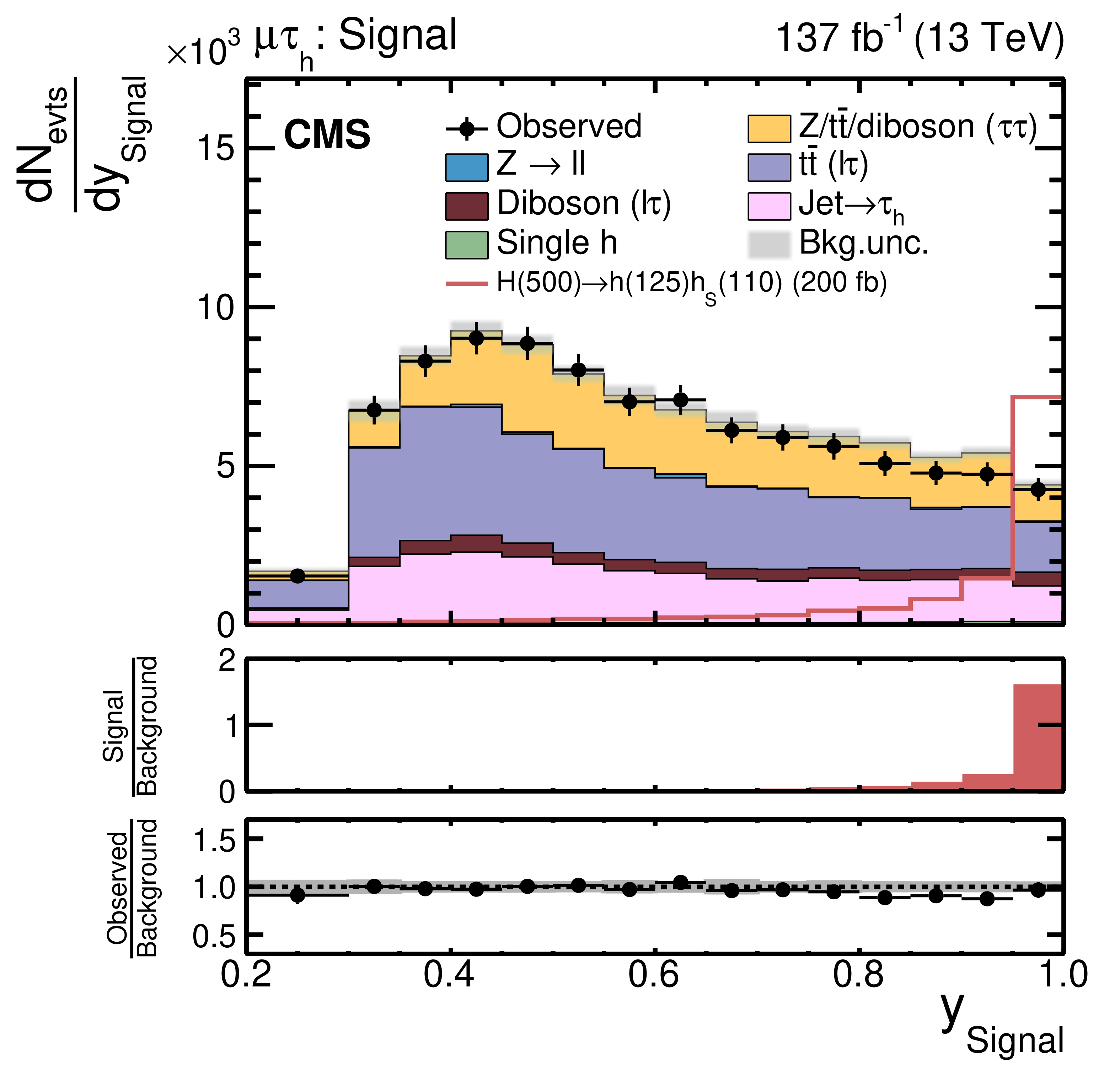
Event categories after NN classification based on a training for $ {m_{\mathrm{H}}} = $ 500 GeV and 100 $\leq {m_{{\mathrm{h} _{\text {S}}}}} < $ 150 GeV in the $\mu {\tau _\mathrm {h}} $ final state. Shown are the (upper left) $\tau \tau $, (upper right) tt, (middle left) $ {\text {jet}\to {\tau _\mathrm {h}}}$, (middle right) misc, and (lower left) signal categories. For these figures the data sets of all years have been combined. The uncertainty bands correspond to the combination of statistical and systematic uncertainties after the fit to the signal plus background hypothesis for $ {m_{\mathrm{H}}} = $ 500 GeV and $ {m_{{\mathrm{h} _{\text {S}}}}} = $ 110 GeV. |
png pdf |
Figure 3-a:
Shown is the $\tau \tau $ category, obtained by NN classification based on a training for $ {m_{\mathrm{H}}} = $ 500 GeV and 100 $\leq {m_{{\mathrm{h} _{\text {S}}}}} < $ 150 GeV in the $\mu {\tau _\mathrm {h}} $ final state. The data sets of all years have been combined. The uncertainty bands correspond to the combination of statistical and systematic uncertainties after the fit to the signal plus background hypothesis for $ {m_{\mathrm{H}}} = $ 500 GeV and $ {m_{{\mathrm{h} _{\text {S}}}}} = $ 110 GeV. |
png pdf |
Figure 3-b:
Shown is the tt category, obtained by NN classification based on a training for $ {m_{\mathrm{H}}} = $ 500 GeV and 100 $\leq {m_{{\mathrm{h} _{\text {S}}}}} < $ 150 GeV in the $\mu {\tau _\mathrm {h}} $ final state. The data sets of all years have been combined. The uncertainty bands correspond to the combination of statistical and systematic uncertainties after the fit to the signal plus background hypothesis for $ {m_{\mathrm{H}}} = $ 500 GeV and $ {m_{{\mathrm{h} _{\text {S}}}}} = $ 110 GeV. |

png pdf |
Figure 3-c:
Shown is the $ {\text {jet}\to {\tau _\mathrm {h}}}$ category, obtained by NN classification based on a training for $ {m_{\mathrm{H}}} = $ 500 GeV and 100 $\leq {m_{{\mathrm{h} _{\text {S}}}}} < $ 150 GeV in the $\mu {\tau _\mathrm {h}} $ final state. The data sets of all years have been combined. The uncertainty bands correspond to the combination of statistical and systematic uncertainties after the fit to the signal plus background hypothesis for $ {m_{\mathrm{H}}} = $ 500 GeV and $ {m_{{\mathrm{h} _{\text {S}}}}} = $ 110 GeV. |
png pdf |
Figure 3-d:
Shown is the misc category, obtained by NN classification based on a training for $ {m_{\mathrm{H}}} = $ 500 GeV and 100 $\leq {m_{{\mathrm{h} _{\text {S}}}}} < $ 150 GeV in the $\mu {\tau _\mathrm {h}} $ final state. The data sets of all years have been combined. The uncertainty bands correspond to the combination of statistical and systematic uncertainties after the fit to the signal plus background hypothesis for $ {m_{\mathrm{H}}} = $ 500 GeV and $ {m_{{\mathrm{h} _{\text {S}}}}} = $ 110 GeV. |
png pdf |
Figure 3-e:
Shown is the signal category, obtained by NN classification based on a training for $ {m_{\mathrm{H}}} = $ 500 GeV and 100 $\leq {m_{{\mathrm{h} _{\text {S}}}}} < $ 150 GeV in the $\mu {\tau _\mathrm {h}} $ final state. The data sets of all years have been combined. The uncertainty bands correspond to the combination of statistical and systematic uncertainties after the fit to the signal plus background hypothesis for $ {m_{\mathrm{H}}} = $ 500 GeV and $ {m_{{\mathrm{h} _{\text {S}}}}} = $ 110 GeV. |

png pdf |
Figure 4:
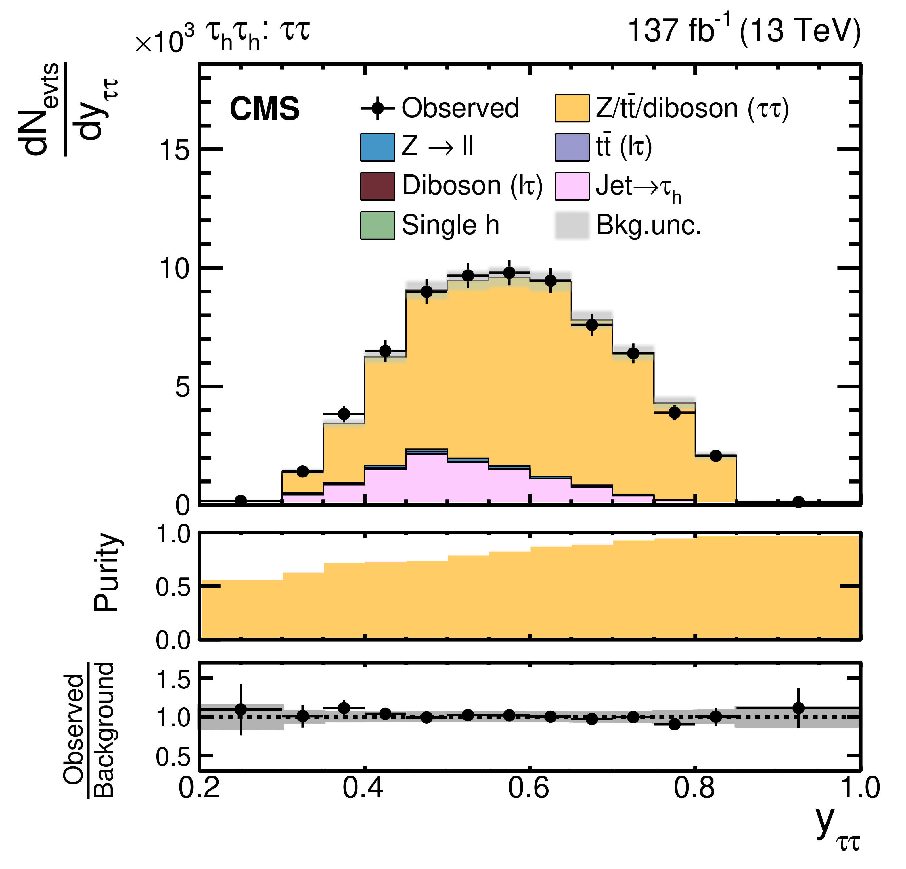
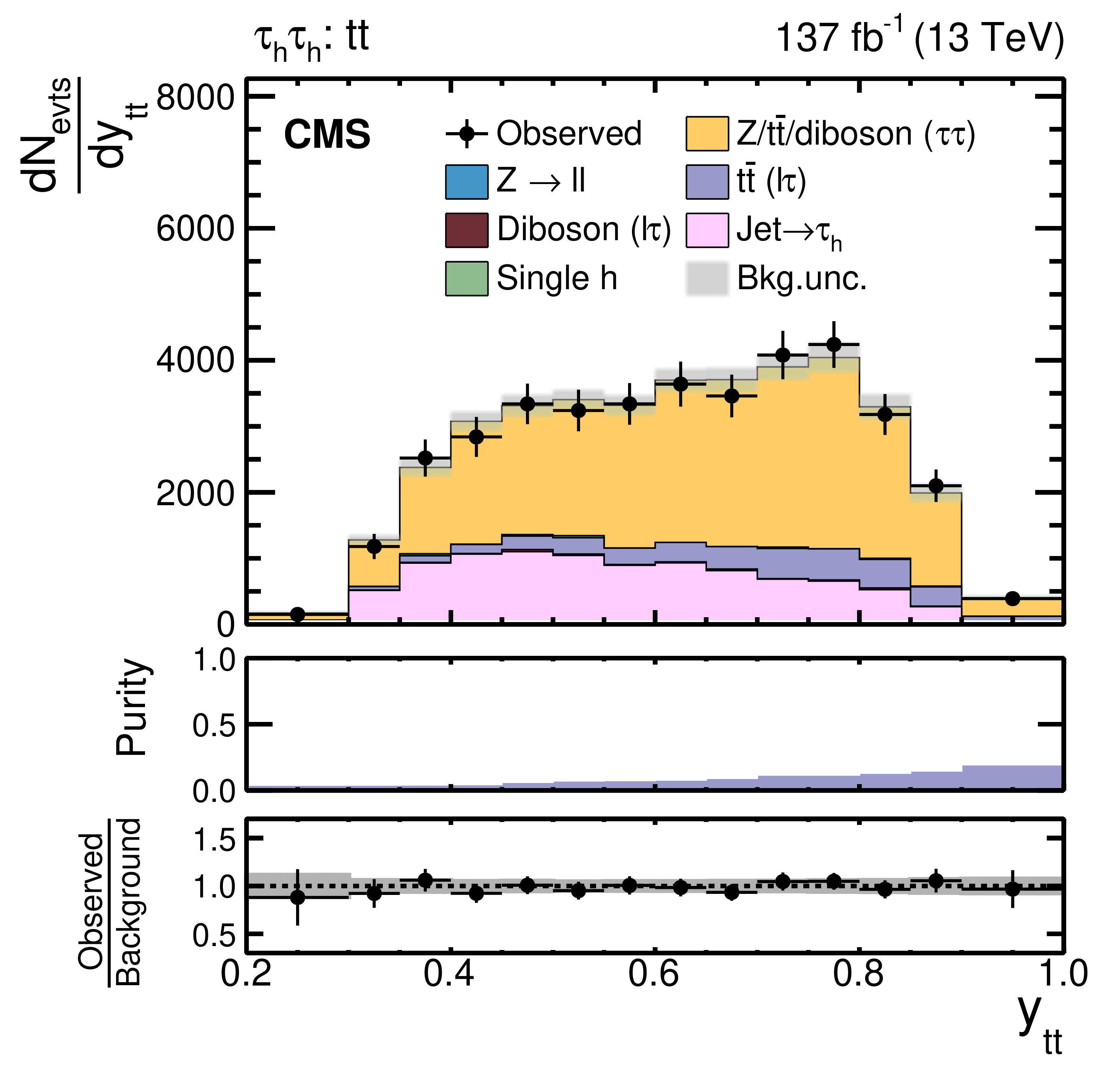
Event categories after NN classification based on a training for $ {m_{\mathrm{H}}} = $ 500 GeV and 100 $\leq {m_{{\mathrm{h} _{\text {S}}}}} < $ 150 GeV in the $ {\tau _\mathrm {h}} {\tau _\mathrm {h}} $ final state. Shown are the (upper left) $\tau \tau $, (upper right) tt, (middle left) $ {\text {jet}\to {\tau _\mathrm {h}}}$, (middle right) misc, and (lower left) signal categories. For these figures the data sets of all years have been combined. The uncertainty bands correspond to the combination of statistical and systematic uncertainties after the fit to the signal plus background hypothesis for $ {m_{\mathrm{H}}} = $ 500 GeV and $ {m_{{\mathrm{h} _{\text {S}}}}} = $ 110 GeV. |
png pdf |
Figure 4-a:
Shown is the $\tau \tau $ category, obtained by NN classification based on a training for $ {m_{\mathrm{H}}} = $ 500 GeV and 100 $\leq {m_{{\mathrm{h} _{\text {S}}}}} < $ 150 GeV in the $ {\tau _\mathrm {h}} {\tau _\mathrm {h}} $ final state. The data sets of all years have been combined. The uncertainty bands correspond to the combination of statistical and systematic uncertainties after the fit to the signal plus background hypothesis for $ {m_{\mathrm{H}}} = $ 500 GeV and $ {m_{{\mathrm{h} _{\text {S}}}}} = $ 110 GeV. |
png pdf |
Figure 4-b:
Shown is the tt category, obtained by NN classification based on a training for $ {m_{\mathrm{H}}} = $ 500 GeV and 100 $\leq {m_{{\mathrm{h} _{\text {S}}}}} < $ 150 GeV in the $ {\tau _\mathrm {h}} {\tau _\mathrm {h}} $ final state. The data sets of all years have been combined. The uncertainty bands correspond to the combination of statistical and systematic uncertainties after the fit to the signal plus background hypothesis for $ {m_{\mathrm{H}}} = $ 500 GeV and $ {m_{{\mathrm{h} _{\text {S}}}}} = $ 110 GeV. |

png pdf |
Figure 4-c:
Shown is the $ {\text {jet}\to {\tau _\mathrm {h}}}$ category, obtained by NN classification based on a training for $ {m_{\mathrm{H}}} = $ 500 GeV and 100 $\leq {m_{{\mathrm{h} _{\text {S}}}}} < $ 150 GeV in the $ {\tau _\mathrm {h}} {\tau _\mathrm {h}} $ final state. The data sets of all years have been combined. The uncertainty bands correspond to the combination of statistical and systematic uncertainties after the fit to the signal plus background hypothesis for $ {m_{\mathrm{H}}} = $ 500 GeV and $ {m_{{\mathrm{h} _{\text {S}}}}} = $ 110 GeV. |

png pdf |
Figure 4-d:
Shown is the misc category, obtained by NN classification based on a training for $ {m_{\mathrm{H}}} = $ 500 GeV and 100 $\leq {m_{{\mathrm{h} _{\text {S}}}}} < $ 150 GeV in the $ {\tau _\mathrm {h}} {\tau _\mathrm {h}} $ final state. The data sets of all years have been combined. The uncertainty bands correspond to the combination of statistical and systematic uncertainties after the fit to the signal plus background hypothesis for $ {m_{\mathrm{H}}} = $ 500 GeV and $ {m_{{\mathrm{h} _{\text {S}}}}} = $ 110 GeV. |

png pdf |
Figure 4-e:
Shown is the signal category, obtained by NN classification based on a training for $ {m_{\mathrm{H}}} = $ 500 GeV and 100 $\leq {m_{{\mathrm{h} _{\text {S}}}}} < $ 150 GeV in the $ {\tau _\mathrm {h}} {\tau _\mathrm {h}} $ final state. The data sets of all years have been combined. The uncertainty bands correspond to the combination of statistical and systematic uncertainties after the fit to the signal plus background hypothesis for $ {m_{\mathrm{H}}} = $ 500 GeV and $ {m_{{\mathrm{h} _{\text {S}}}}} = $ 110 GeV. |
png pdf |
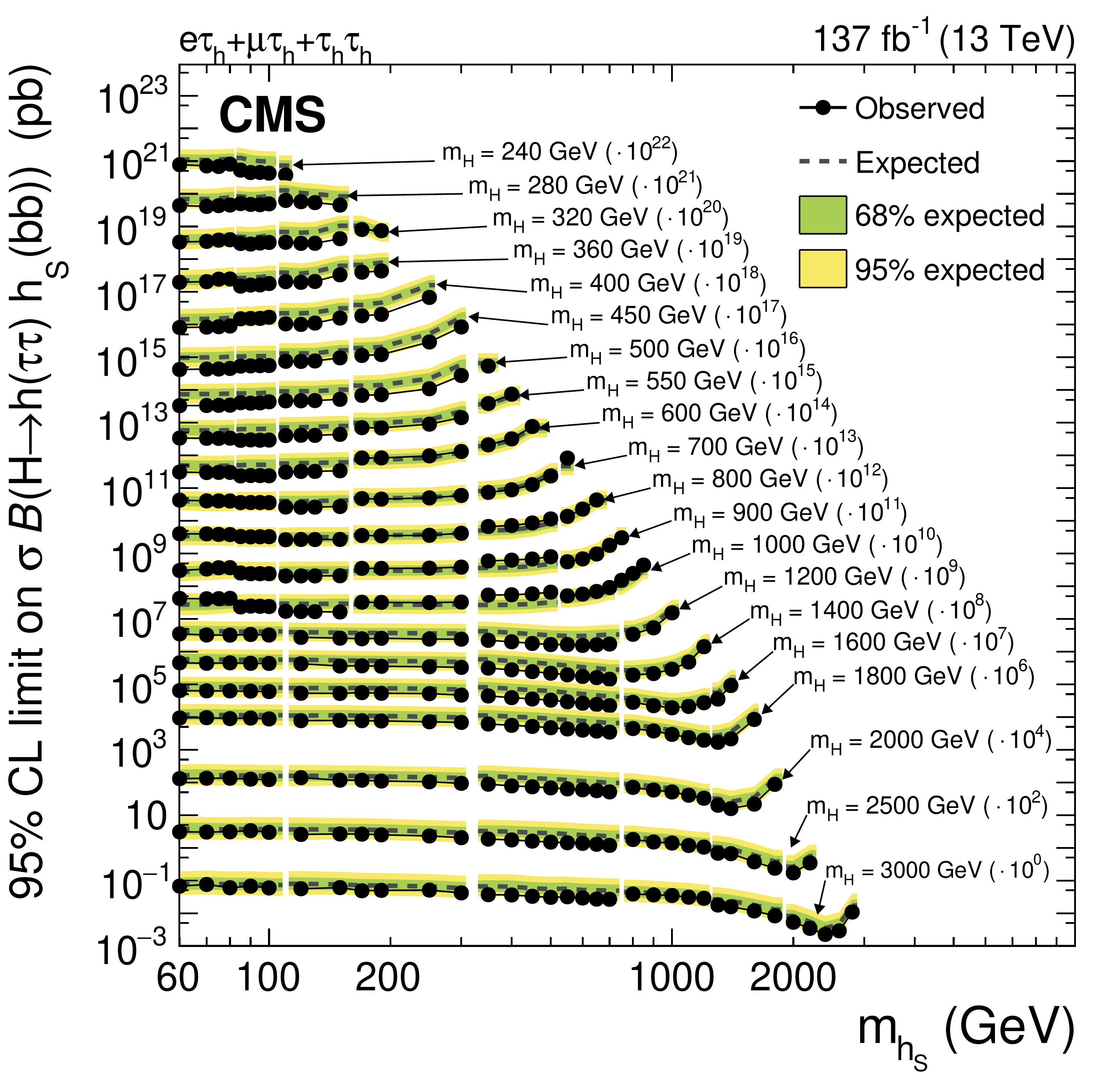
Figure 5:
Expected and observed 95% CL upper limits on $ {\sigma \,\mathcal {B}(\mathrm{H} \to \mathrm{h} (\tau \tau) {\mathrm{h} _{\text {S}}} (\mathrm{b} \mathrm{b}))}$ for all tested values of $ {m_{\mathrm{H}}}$ and $ {m_{{\mathrm{h} _{\text {S}}}}}$. The limits for each corresponding mass value have been scaled by orders of ten as indicated in the annotations. Groups of hypothesis tests based on the same NN trainings for classification are indicated by discontinuities in the limits, which are linearly connected otherwise to improve the visibility of common trends. |
png pdf |
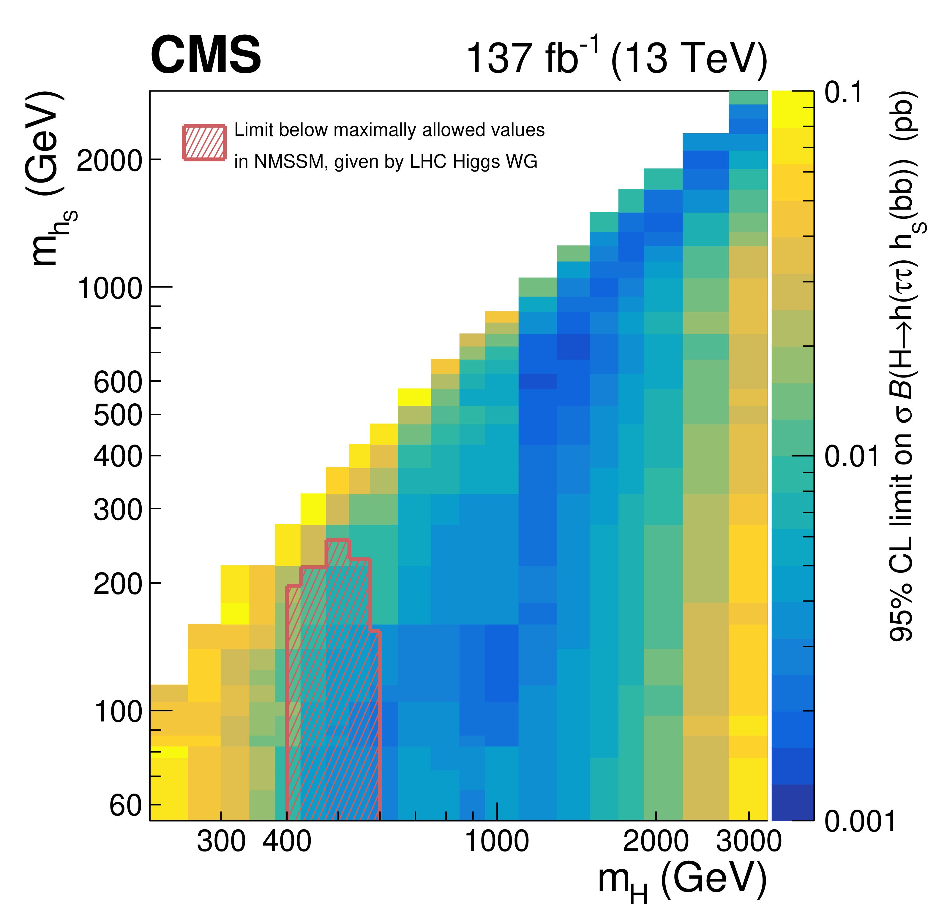
Figure 6:
Summary of the observed limits on $ {\sigma \,\mathcal {B}(\mathrm{H} \to \mathrm{h} (\tau \tau) {\mathrm{h} _{\text {S}}} (\mathrm{b} \mathrm{b}))}$ for all tested pairs of $ {m_{\mathrm{H}}}$ and $ {m_{{\mathrm{h} _{\text {S}}}}}$, as shown in Fig. 5. The limits are given by the color code of the figure. The region in the plane spanned by $ {m_{\mathrm{H}}}$ and $ {m_{{\mathrm{h} _{\text {S}}}}}$ where the observed limits fall below the maximally allowed values on $ {\sigma \,\mathcal {B}(\mathrm{H} \to \mathrm{h} (\tau \tau) {\mathrm{h} _{\text {S}}} (\mathrm{b} \mathrm{b}))}$ in the context of the NMSSM, as provided by the LHC Higgs Working Group, are indicated by a red hatched area. |
| Tables | |
png pdf |
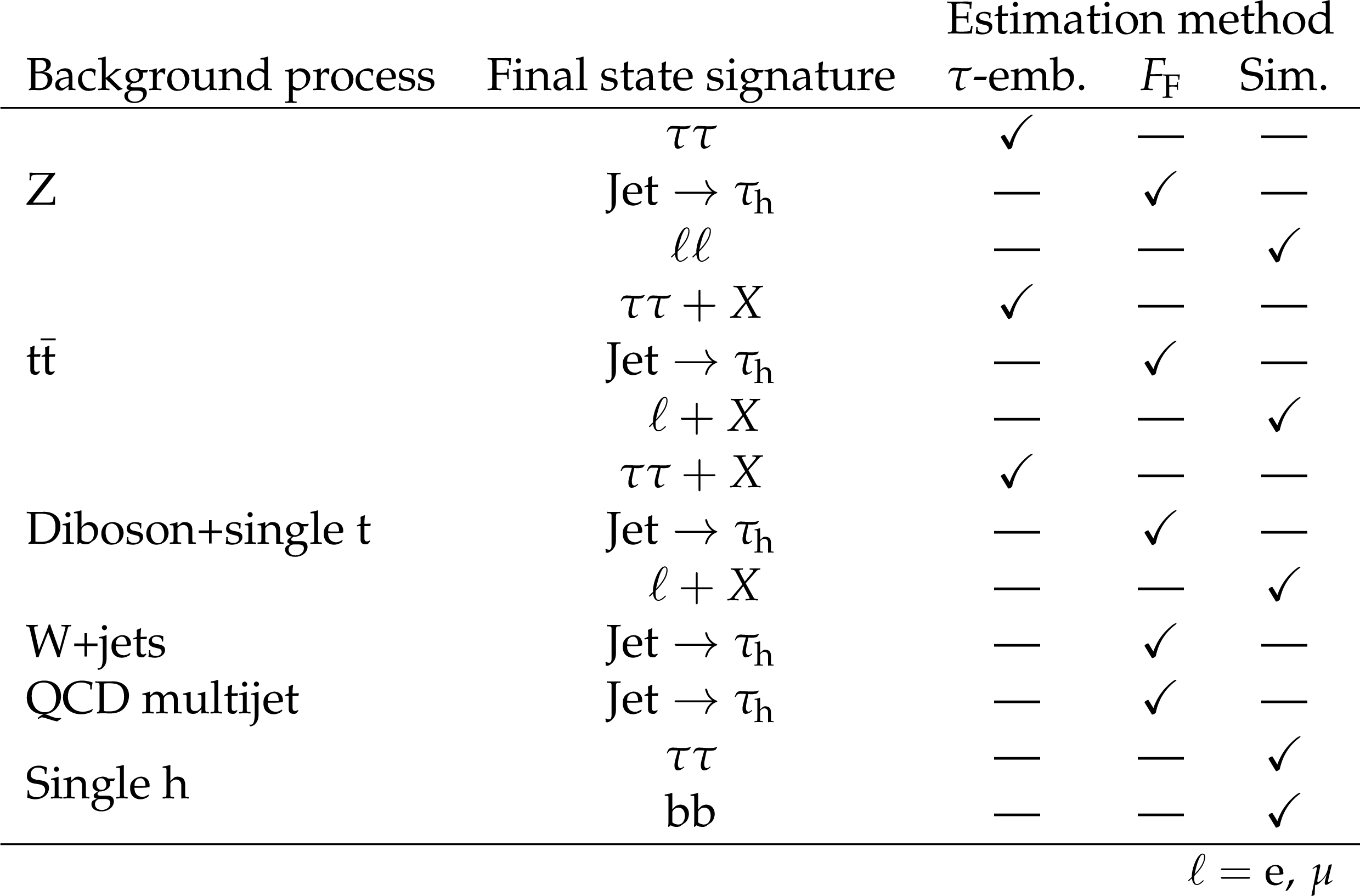
Table 1:
Background processes contributing to the event selection, as given in Section 5. The symbol $\ell $ corresponds to an electron or muon. The second column refers to the experimental signature in the analysis, the last three columns indicate the estimation methods used to model each corresponding signature, as described in Sections 4.1-4.3. |
png pdf |
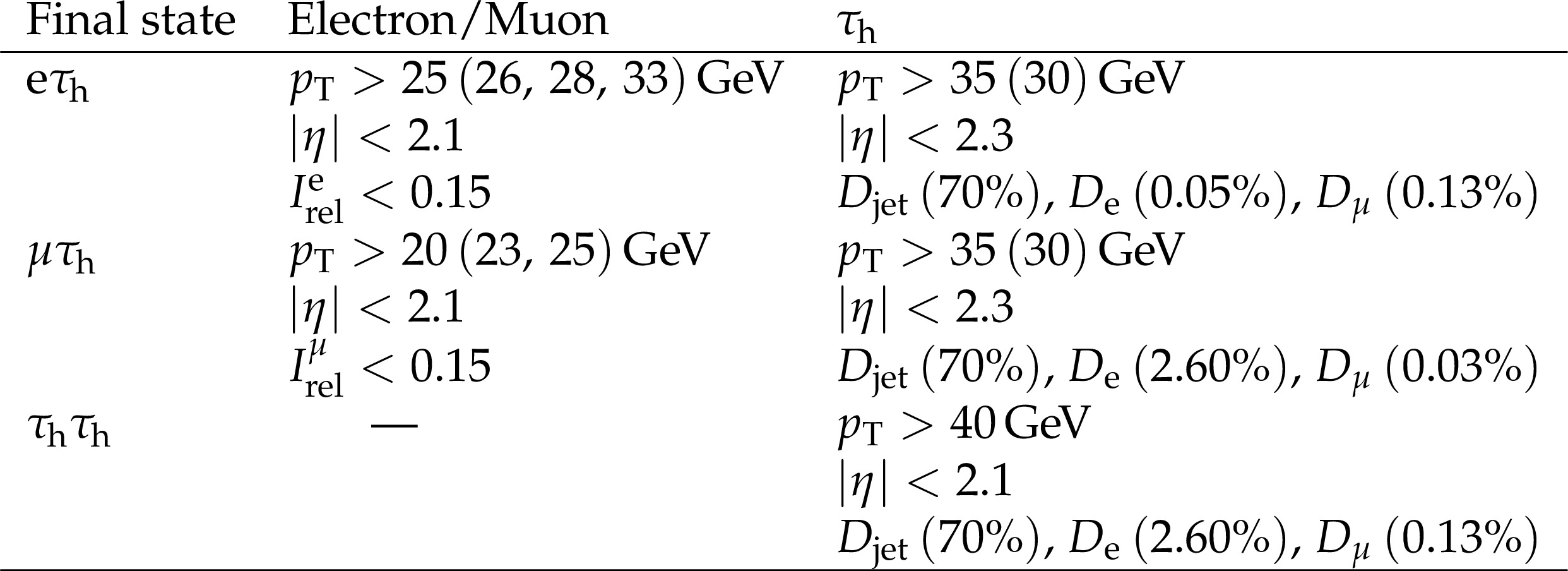
Table 2:
Offline requirements applied to electrons, muons, and $ {\tau _\mathrm {h}} $ candidates used for the selection of the $\tau $ pair. The $ {p_{\mathrm {T}}} $ values in parentheses correspond to events selected by a single-electron or single-muon trigger. These requirements depend on the year of data-taking. For $ {D_{\text {jet}}}$ the efficiency and for $D_{\mathrm{e} (\mu)}$ the misidentification rates for the chosen working points are given in parentheses. A detailed discussion is given in the text. |
png pdf |
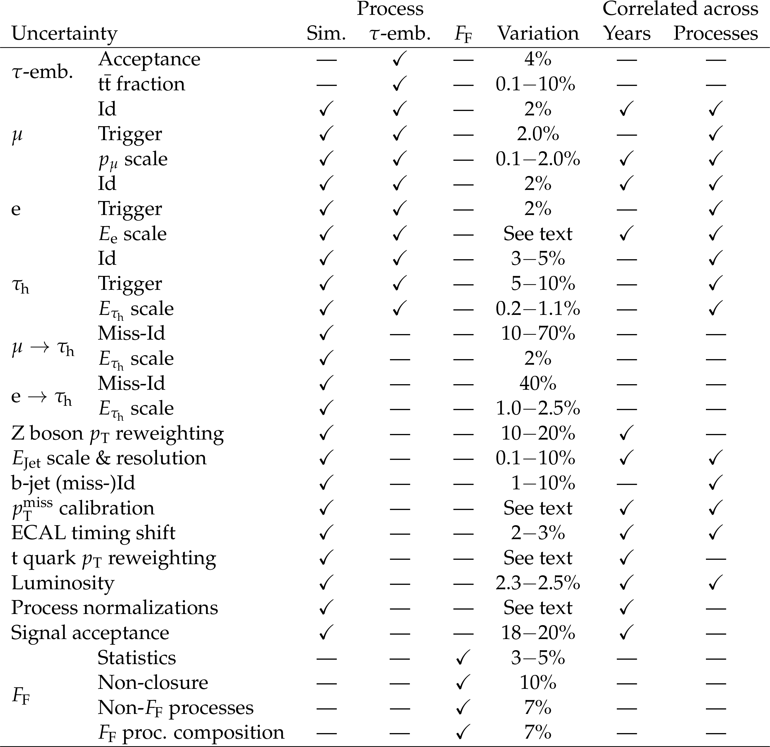
Table 3:
Summary of systematic uncertainties discussed in the text. The first column indicates the source of uncertainty; the second the processes that it applies to; the third the variation; and the last how it is correlated with other uncertainties. A checkmark is given also for partial correlations. More details are given in the text. |
| Summary |
| A search for a heavy Higgs boson H decaying into the observed Higgs boson H with a mass of 125 GeV and another Higgs boson $\mathrm{h_S}$ has been presented. The H and $\mathrm{h_S}$ bosons are required to decay into a pair of tau leptons and a pair of b quarks, respectively. The search uses a sample of proton-proton collisions collected with the CMS detector at a center-of-mass energy of 13 TeV, corresponding to an integrated luminosity of 137 fb$^{-1}$ . Mass ranges of 240-3000 GeV for ${m_{\mathrm{H}}}$ and 60-2800 GeV for ${m_{\mathrm{h_S}}}$ are explored in the search. No signal has been observed. Model independent 95% confidence level upper limits on the product of the production cross section and the branching fractions of the signal process are set with a sensitivity ranging from 125 fb (for ${m_{\mathrm{H}}} = $ 240 GeV) to 2.7 fb (for ${m_{\mathrm{H}}} = $ 1000 GeV). These limits have been compared to maximally allowed products of the production cross section and the branching fractions of the signal process in the next-to-minimal supersymmetric extension of the standard model. This is the first search for such a process carried out at the LHC. |
| Additional Figures | |
png pdf |
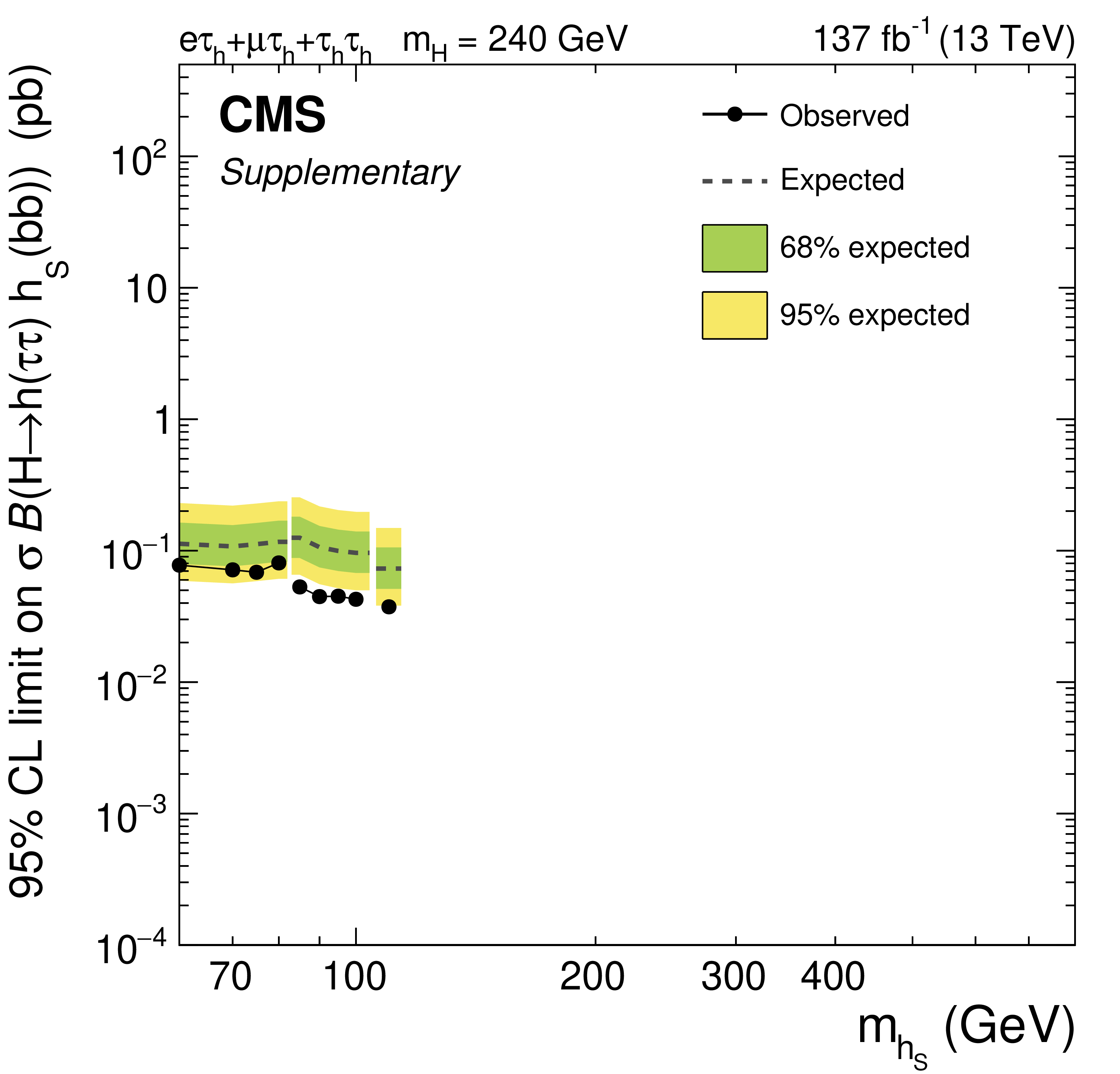
Additional Figure 1:
Expected and observed 95% confidence level upper limits on $ {\sigma \,\mathcal {B}({\mathrm {H}} \to {\mathrm {h}} ({\tau} {\tau}) {{\mathrm {h}} _{\text {S}}} ({\mathrm {b}} {\mathrm {b}}))}$ for $ {m_{{\mathrm {H}}}} = $ 240 GeV and 60 $\leq {m_{{{\mathrm {h}} _{\text {S}}}}}\leq $ 110 GeV. |
png pdf |
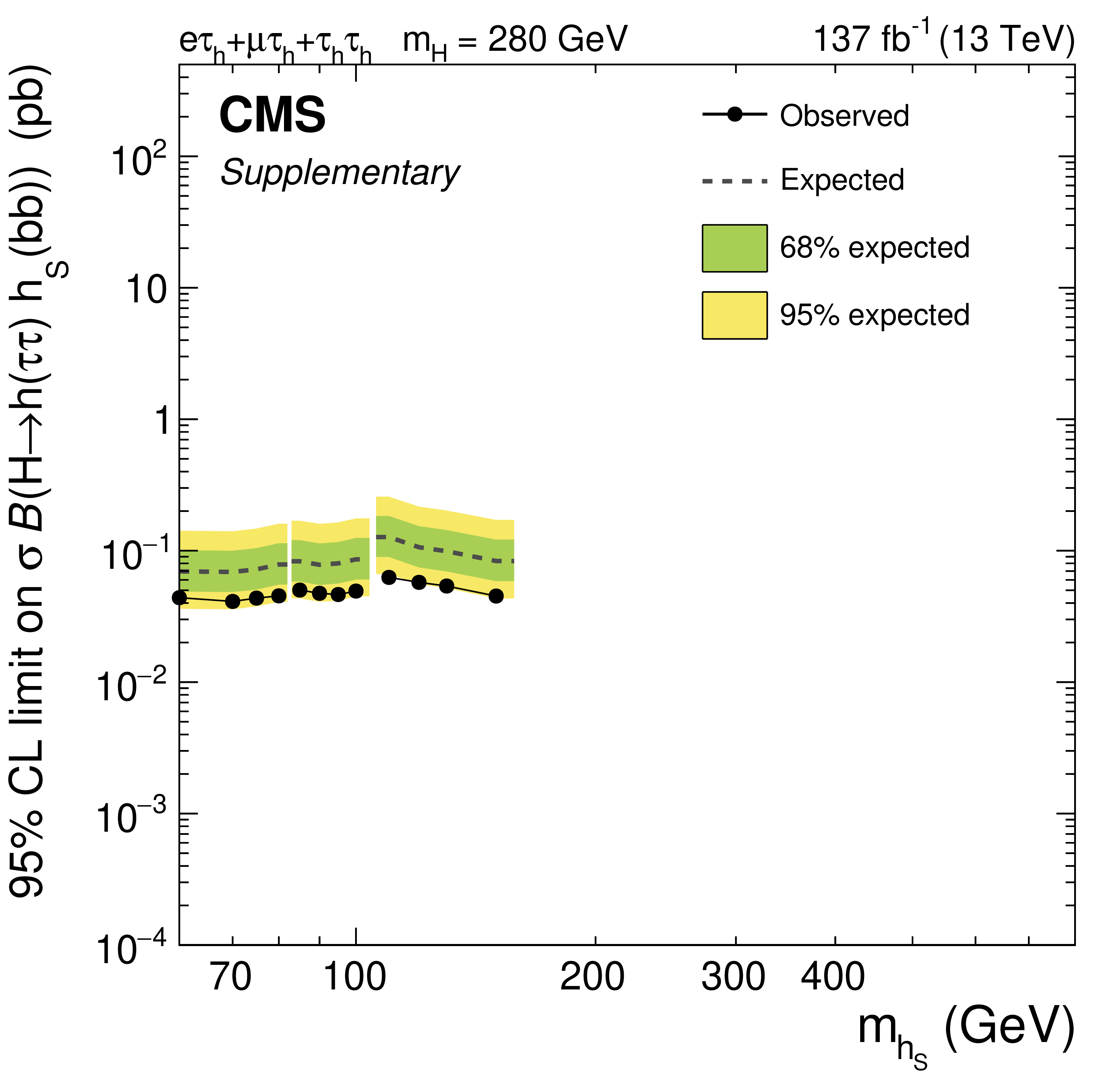
Additional Figure 2:
Expected and observed 95% confidence level upper limits on $ {\sigma \,\mathcal {B}({\mathrm {H}} \to {\mathrm {h}} ({\tau} {\tau}) {{\mathrm {h}} _{\text {S}}} ({\mathrm {b}} {\mathrm {b}}))}$ for $ {m_{{\mathrm {H}}}} = $ 280 GeV and 60 $\leq {m_{{{\mathrm {h}} _{\text {S}}}}}\leq $ 150 GeV. |
png pdf |
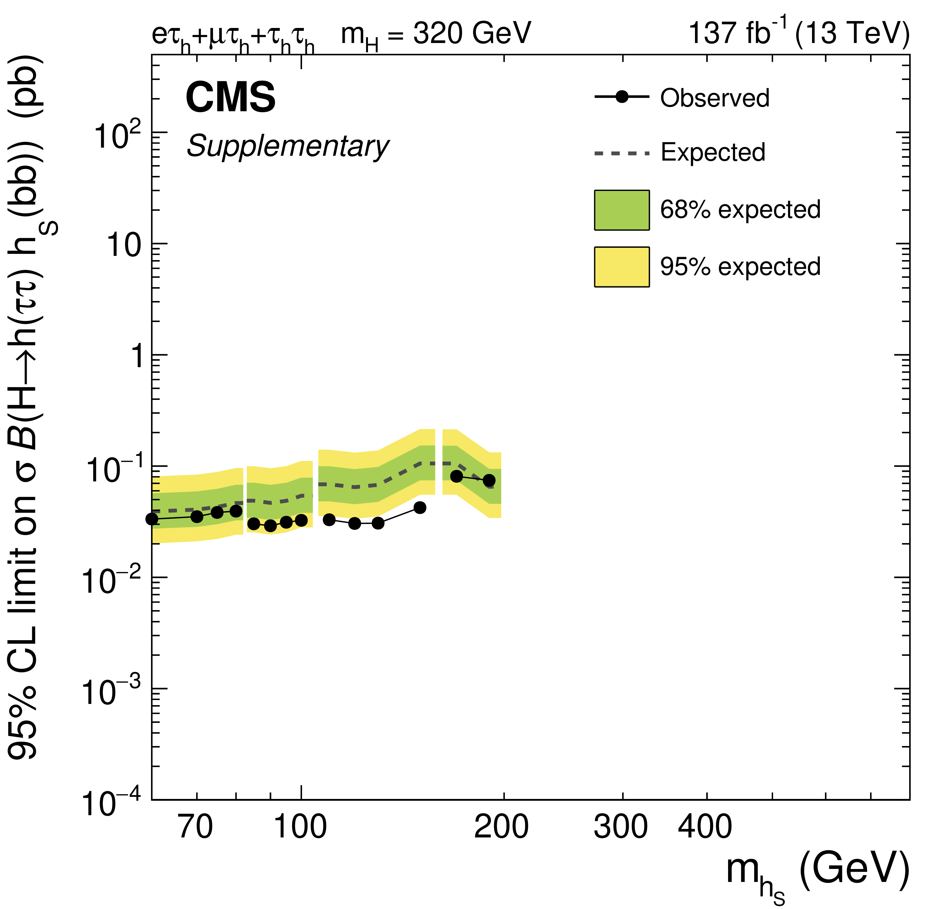
Additional Figure 3:
Expected and observed 95% confidence level upper limits on $ {\sigma \,\mathcal {B}({\mathrm {H}} \to {\mathrm {h}} ({\tau} {\tau}) {{\mathrm {h}} _{\text {S}}} ({\mathrm {b}} {\mathrm {b}}))}$ for $ {m_{{\mathrm {H}}}} = $ 320 GeV and 60 $\leq {m_{{{\mathrm {h}} _{\text {S}}}}}\leq $ 190 GeV. |

png pdf |
Additional Figure 4:
Expected and observed 95% confidence level upper limits on $ {\sigma \,\mathcal {B}({\mathrm {H}} \to {\mathrm {h}} ({\tau} {\tau}) {{\mathrm {h}} _{\text {S}}} ({\mathrm {b}} {\mathrm {b}}))}$ for $ {m_{{\mathrm {H}}}} = $ 360 GeV and 60 $\leq {m_{{{\mathrm {h}} _{\text {S}}}}}\leq $ 190 GeV. |

png pdf |
Additional Figure 5:
Expected and observed 95% confidence level upper limits on $ {\sigma \,\mathcal {B}({\mathrm {H}} \to {\mathrm {h}} ({\tau} {\tau}) {{\mathrm {h}} _{\text {S}}} ({\mathrm {b}} {\mathrm {b}}))}$ for $ {m_{{\mathrm {H}}}} = $ 400 GeV and 60 $\leq {m_{{{\mathrm {h}} _{\text {S}}}}}\leq $ 250 GeV. |
png pdf |
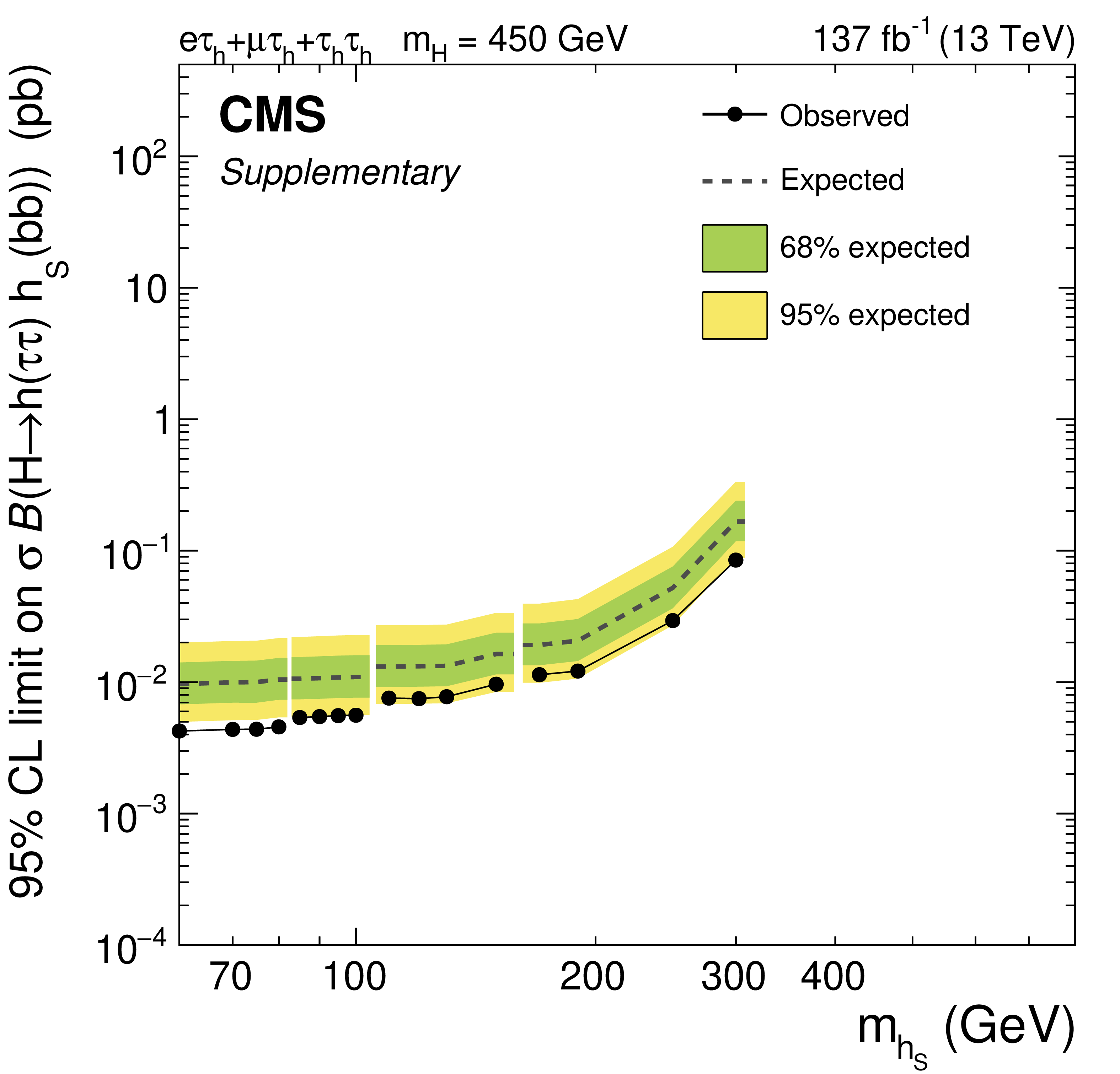
Additional Figure 6:
Expected and observed 95% confidence level upper limits on $ {\sigma \,\mathcal {B}({\mathrm {H}} \to {\mathrm {h}} ({\tau} {\tau}) {{\mathrm {h}} _{\text {S}}} ({\mathrm {b}} {\mathrm {b}}))}$ for $ {m_{{\mathrm {H}}}} = $ 450 GeV and 60 $\leq {m_{{{\mathrm {h}} _{\text {S}}}}}\leq $ 300 GeV. |
png pdf |
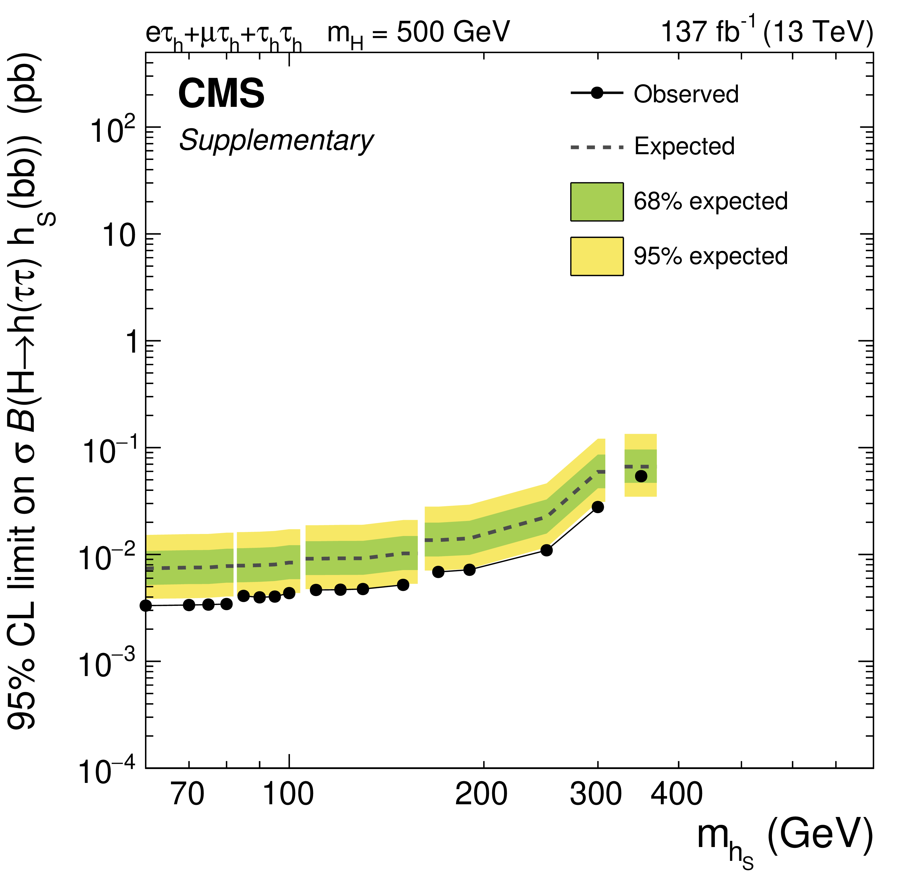
Additional Figure 7:
Expected and observed 95% confidence level upper limits on $ {\sigma \,\mathcal {B}({\mathrm {H}} \to {\mathrm {h}} ({\tau} {\tau}) {{\mathrm {h}} _{\text {S}}} ({\mathrm {b}} {\mathrm {b}}))}$ for $ {m_{{\mathrm {H}}}} = $ 500 GeV and 60 $\leq {m_{{{\mathrm {h}} _{\text {S}}}}}\leq $ 350 GeV. |
png pdf |
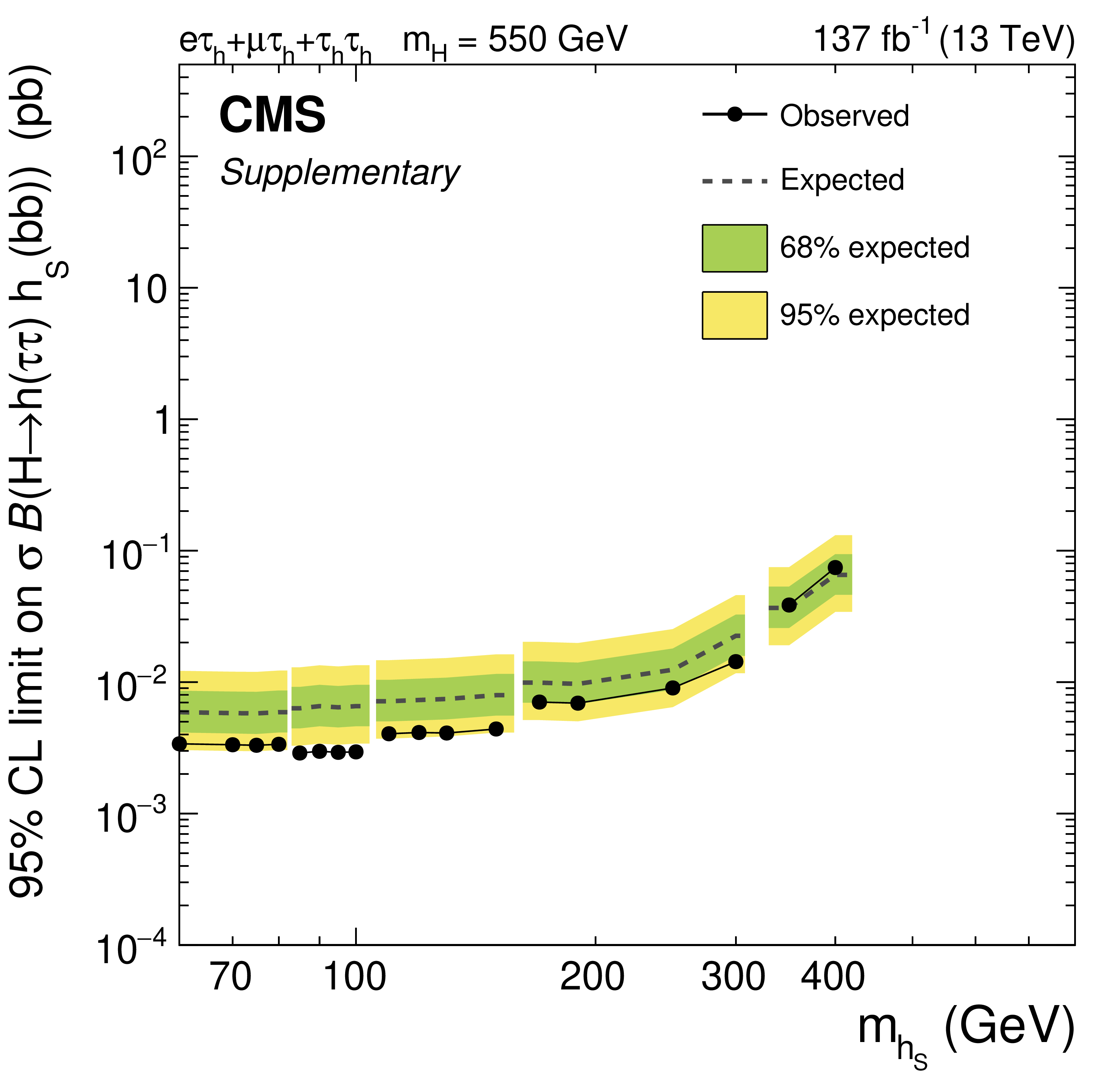
Additional Figure 8:
Expected and observed 95% confidence level upper limits on $ {\sigma \,\mathcal {B}({\mathrm {H}} \to {\mathrm {h}} ({\tau} {\tau}) {{\mathrm {h}} _{\text {S}}} ({\mathrm {b}} {\mathrm {b}}))}$ for $ {m_{{\mathrm {H}}}} = $ 550 GeV and 60 $\leq {m_{{{\mathrm {h}} _{\text {S}}}}}\leq $ 400 GeV. |

png pdf |
Additional Figure 9:
Expected and observed 95% confidence level upper limits on $ {\sigma \,\mathcal {B}({\mathrm {H}} \to {\mathrm {h}} ({\tau} {\tau}) {{\mathrm {h}} _{\text {S}}} ({\mathrm {b}} {\mathrm {b}}))}$ for $ {m_{{\mathrm {H}}}} = $ 600 GeV and 60 $\leq {m_{{{\mathrm {h}} _{\text {S}}}}}\leq $ 450 GeV. |
png pdf |
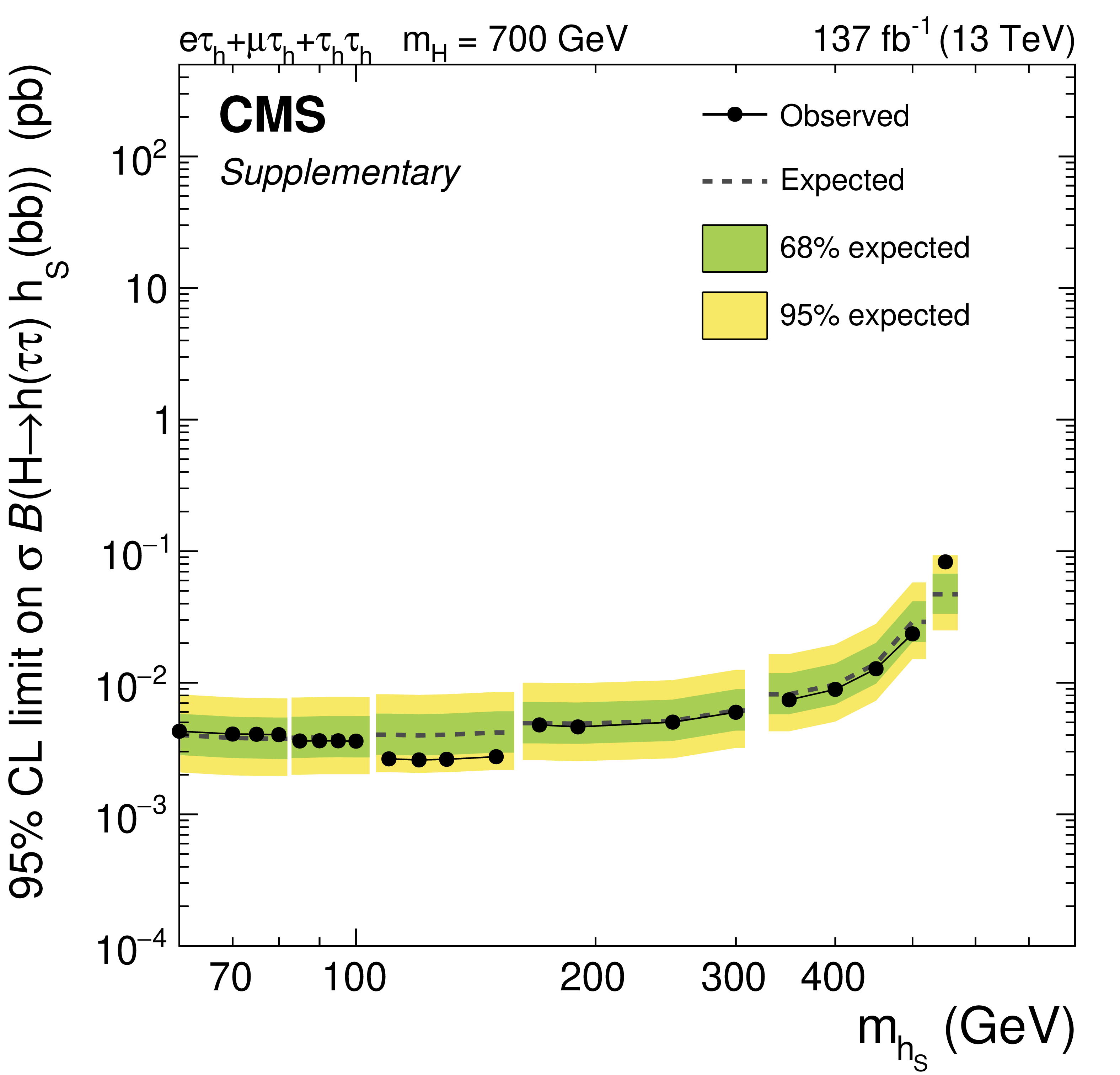
Additional Figure 10:
Expected and observed 95% confidence level upper limits on $ {\sigma \,\mathcal {B}({\mathrm {H}} \to {\mathrm {h}} ({\tau} {\tau}) {{\mathrm {h}} _{\text {S}}} ({\mathrm {b}} {\mathrm {b}}))}$ for $ {m_{{\mathrm {H}}}} = $ 700 GeV and 60 $\leq {m_{{{\mathrm {h}} _{\text {S}}}}}\leq $ 550 GeV. |
png pdf |
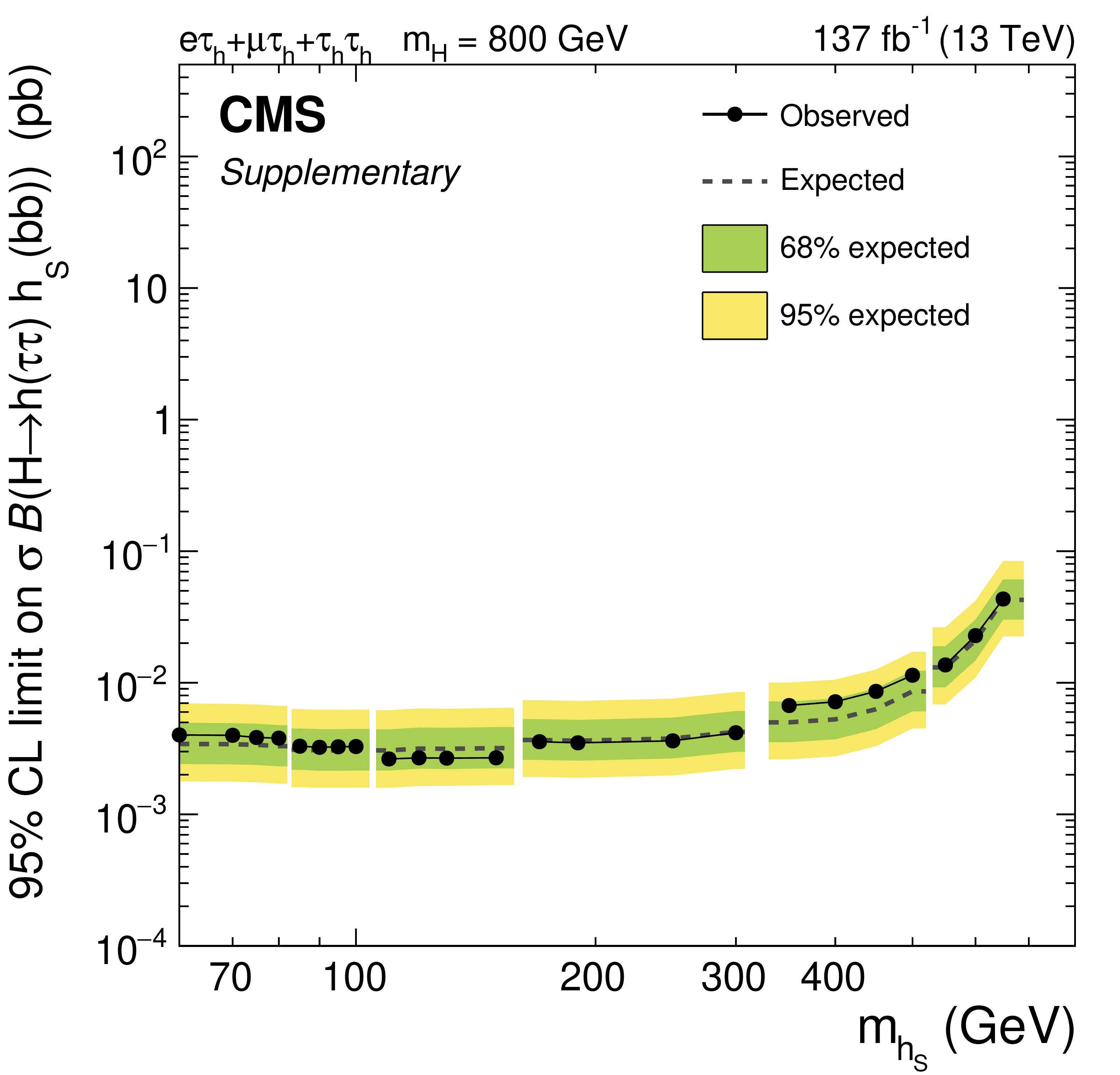
Additional Figure 11:
Expected and observed 95% confidence level upper limits on $ {\sigma \,\mathcal {B}({\mathrm {H}} \to {\mathrm {h}} ({\tau} {\tau}) {{\mathrm {h}} _{\text {S}}} ({\mathrm {b}} {\mathrm {b}}))}$ for $ {m_{{\mathrm {H}}}} = $ 800 GeV and 60 $\leq {m_{{{\mathrm {h}} _{\text {S}}}}}\leq $ 650 GeV. |
png pdf |
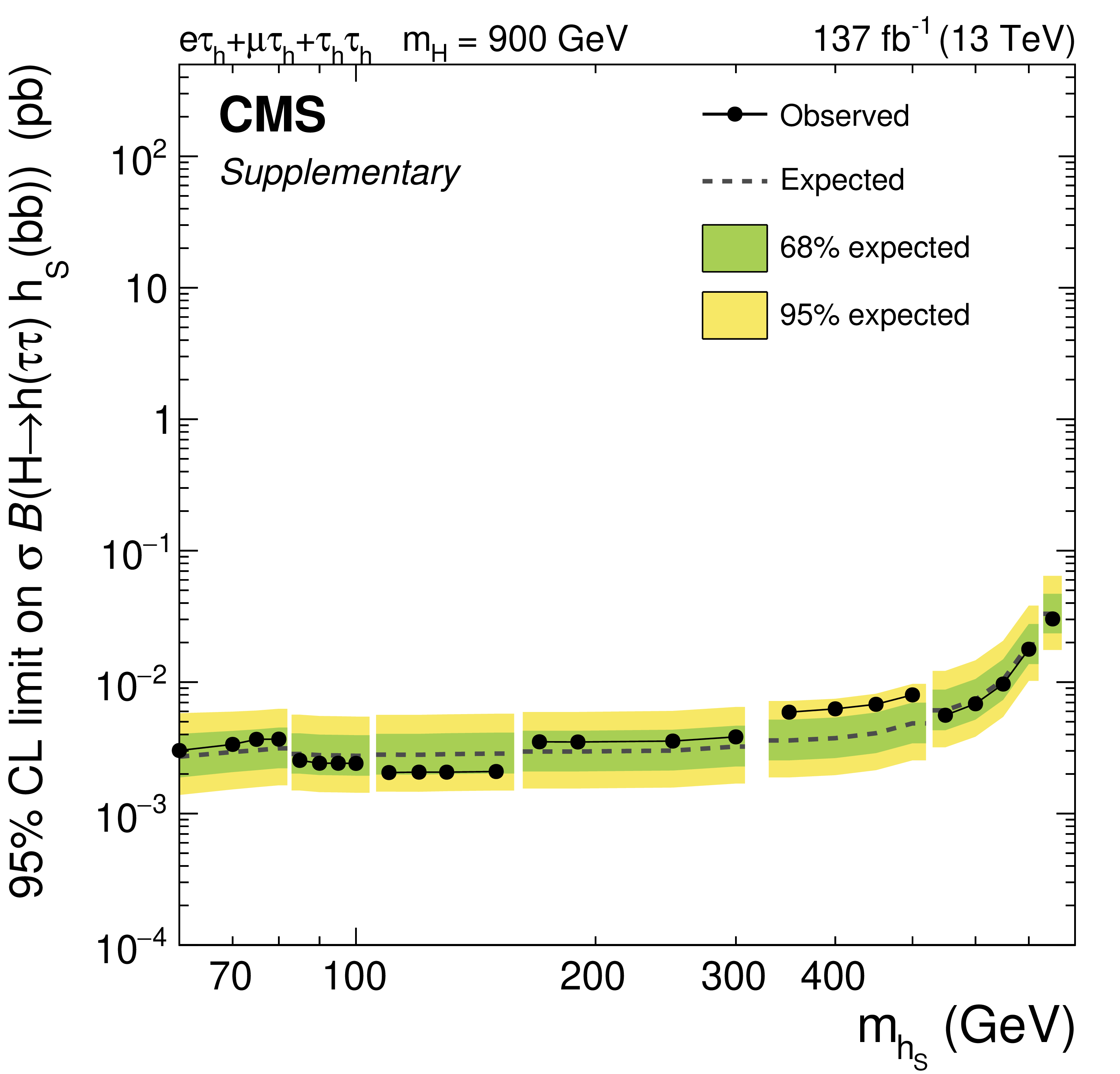
Additional Figure 12:
Expected and observed 95% confidence level upper limits on $ {\sigma \,\mathcal {B}({\mathrm {H}} \to {\mathrm {h}} ({\tau} {\tau}) {{\mathrm {h}} _{\text {S}}} ({\mathrm {b}} {\mathrm {b}}))}$ for $ {m_{{\mathrm {H}}}} = $ 900 GeV and 60 $\leq {m_{{{\mathrm {h}} _{\text {S}}}}}\leq $ 750 GeV. |
png pdf |
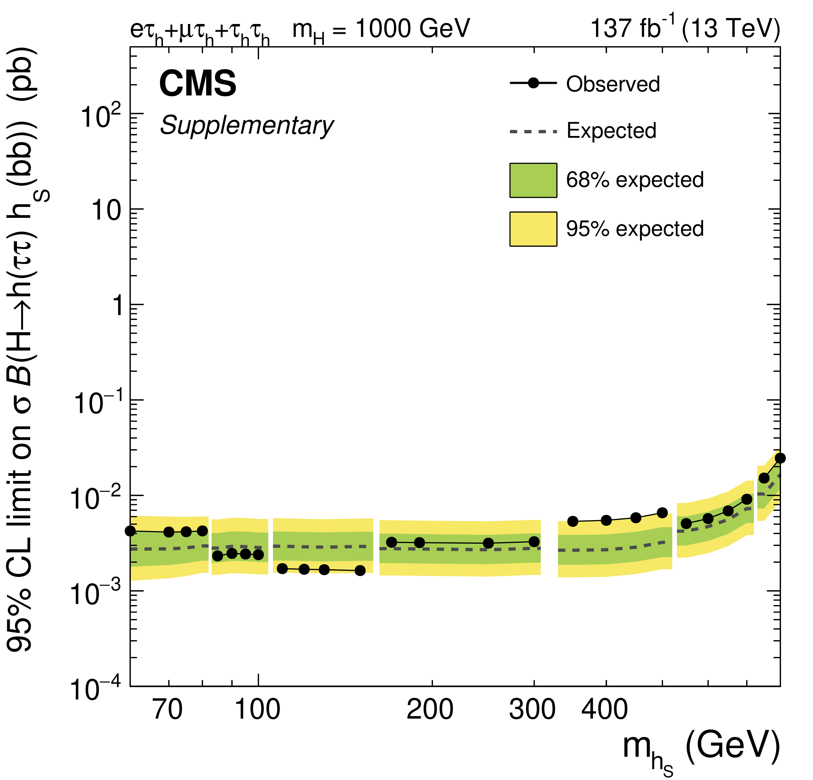
Additional Figure 13:
Expected and observed 95% confidence level upper limits on $ {\sigma \,\mathcal {B}({\mathrm {H}} \to {\mathrm {h}} ({\tau} {\tau}) {{\mathrm {h}} _{\text {S}}} ({\mathrm {b}} {\mathrm {b}}))}$ for $ {m_{{\mathrm {H}}}} = $ 1000 GeV and 60 $\leq {m_{{{\mathrm {h}} _{\text {S}}}}}\leq $ 850 GeV. |
png pdf |
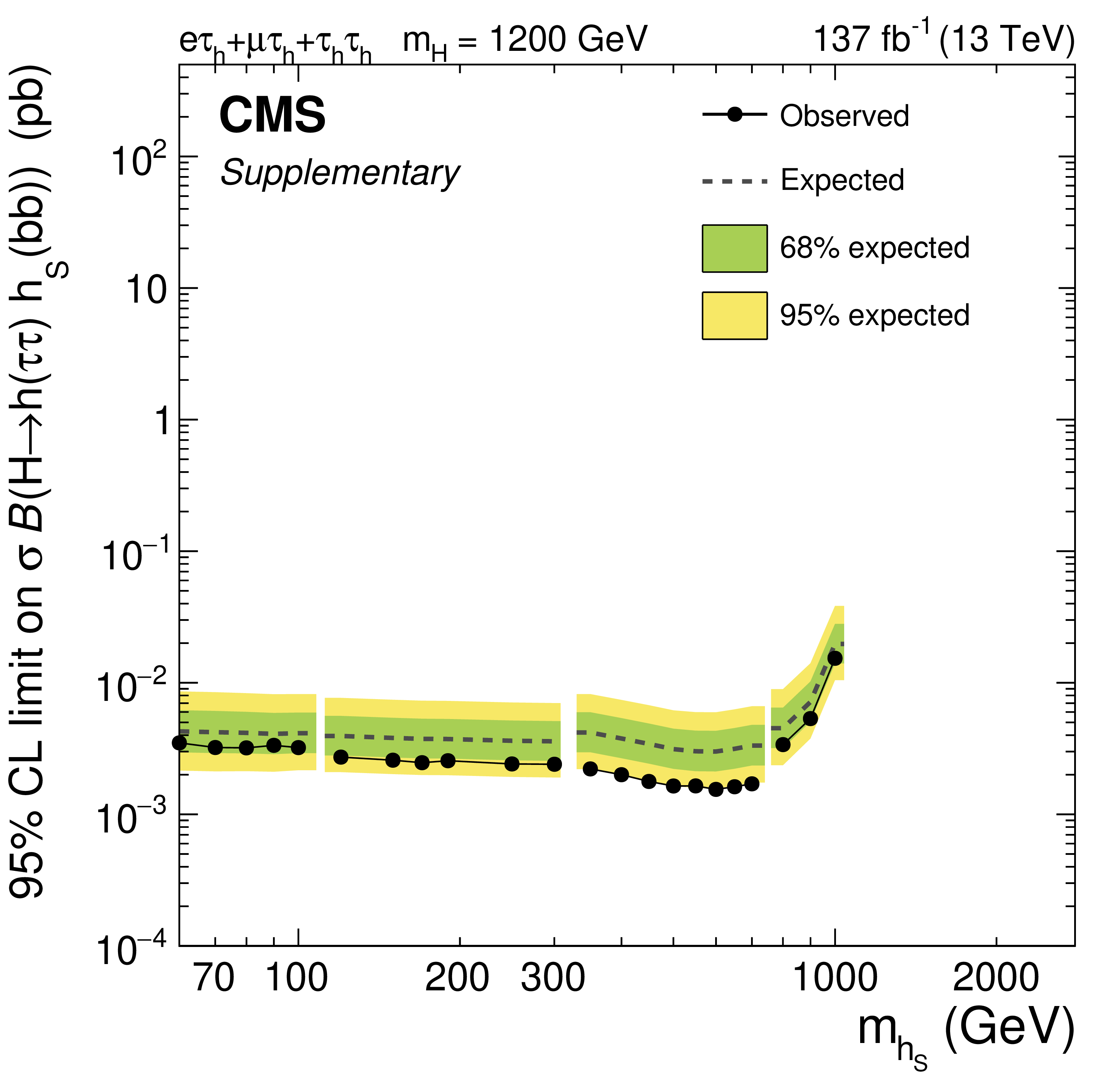
Additional Figure 14:
Expected and observed 95% confidence level upper limits on $ {\sigma \,\mathcal {B}({\mathrm {H}} \to {\mathrm {h}} ({\tau} {\tau}) {{\mathrm {h}} _{\text {S}}} ({\mathrm {b}} {\mathrm {b}}))}$ for $ {m_{{\mathrm {H}}}} = $ 1200 GeV and 60 $\leq {m_{{{\mathrm {h}} _{\text {S}}}}}\leq $ 1000 GeV. |
png pdf |
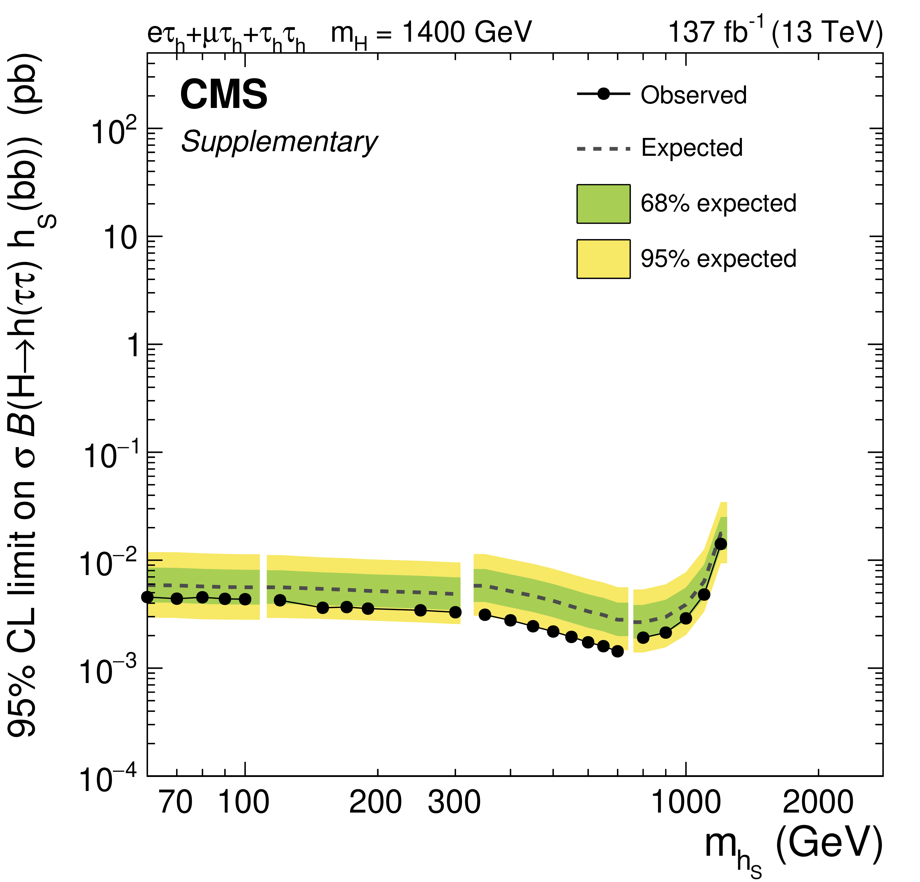
Additional Figure 15:
Expected and observed 95% confidence level upper limits on $ {\sigma \,\mathcal {B}({\mathrm {H}} \to {\mathrm {h}} ({\tau} {\tau}) {{\mathrm {h}} _{\text {S}}} ({\mathrm {b}} {\mathrm {b}}))}$ for $ {m_{{\mathrm {H}}}} = $ 1400 GeV and 60 $\leq {m_{{{\mathrm {h}} _{\text {S}}}}}\leq 1200 GeV $. |

png pdf |
Additional Figure 16:
Expected and observed 95% confidence level upper limits on $ {\sigma \,\mathcal {B}({\mathrm {H}} \to {\mathrm {h}} ({\tau} {\tau}) {{\mathrm {h}} _{\text {S}}} ({\mathrm {b}} {\mathrm {b}}))}$ for $ {m_{{\mathrm {H}}}} = $ 1600 GeV and 60 $\leq {m_{{{\mathrm {h}} _{\text {S}}}}}\leq $ 1400 GeV. |
png pdf |
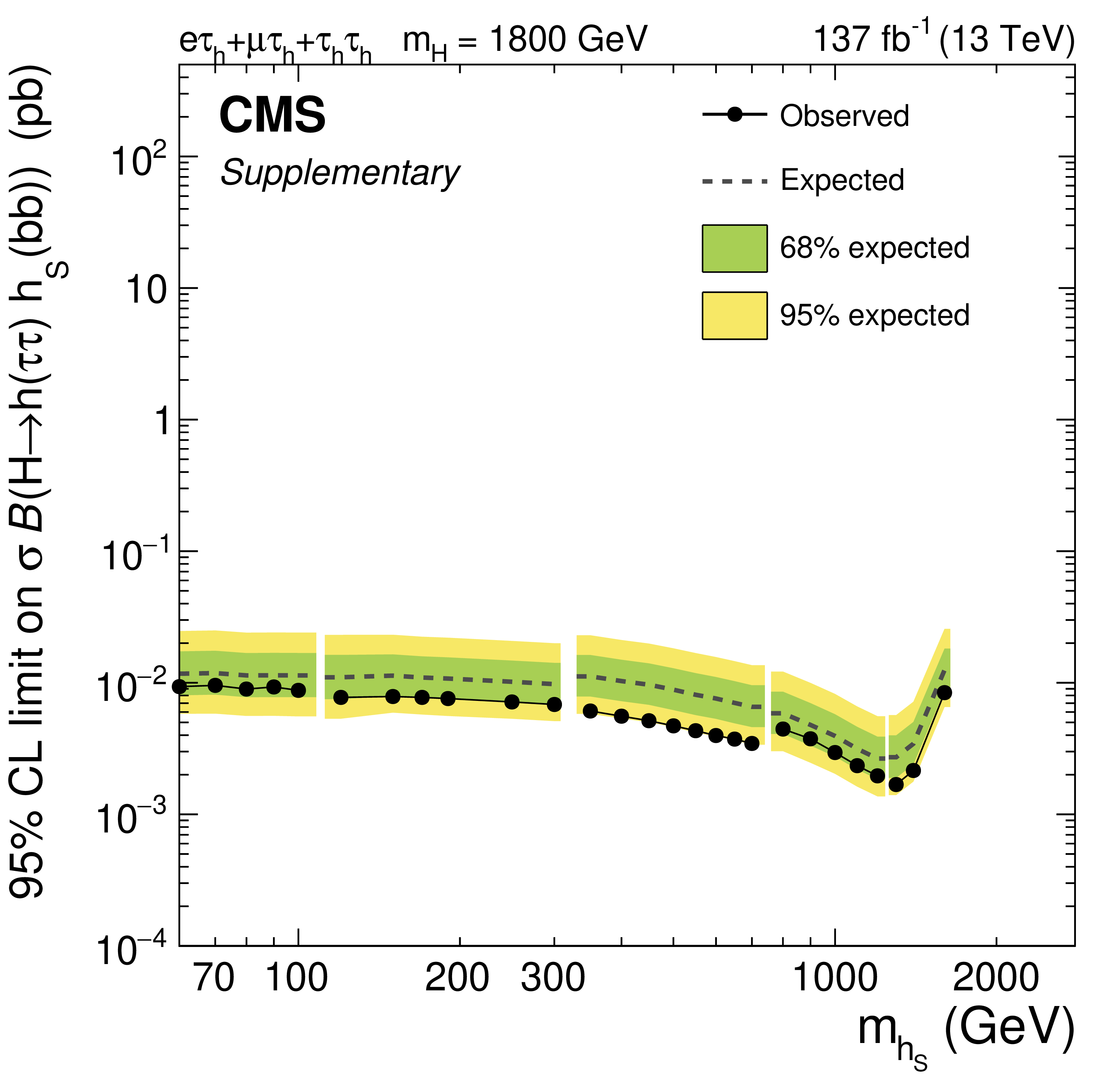
Additional Figure 17:
Expected and observed 95% confidence level upper limits on $ {\sigma \,\mathcal {B}({\mathrm {H}} \to {\mathrm {h}} ({\tau} {\tau}) {{\mathrm {h}} _{\text {S}}} ({\mathrm {b}} {\mathrm {b}}))}$ for $ {m_{{\mathrm {H}}}} = $ 1800 GeV and 60 $\leq {m_{{{\mathrm {h}} _{\text {S}}}}}\leq $ 1600 GeV. |
png pdf |
Additional Figure 18:
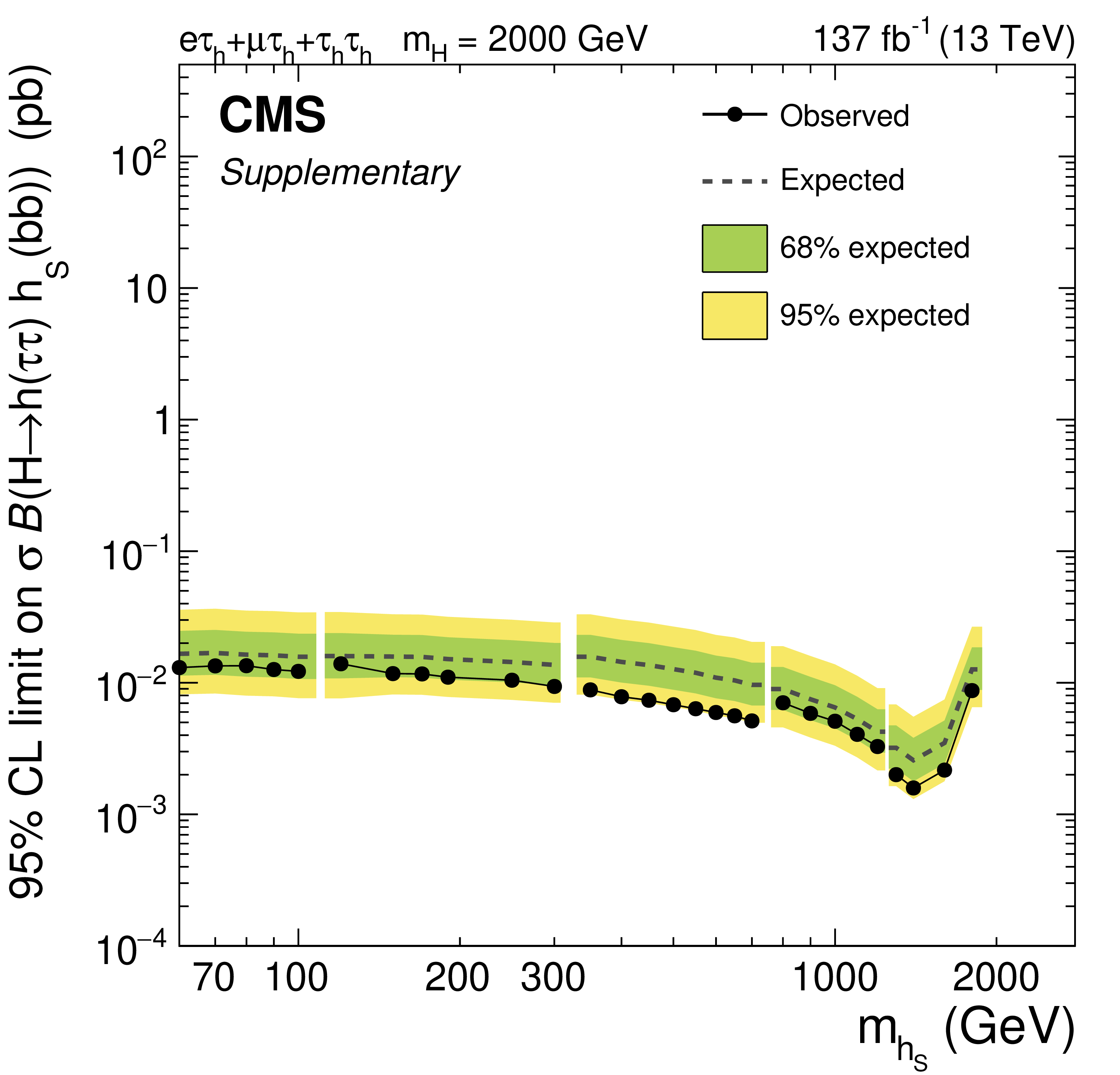
Expected and observed 95% confidence level upper limits on $ {\sigma \,\mathcal {B}({\mathrm {H}} \to {\mathrm {h}} ({\tau} {\tau}) {{\mathrm {h}} _{\text {S}}} ({\mathrm {b}} {\mathrm {b}}))}$ for $ {m_{{\mathrm {H}}}} = $ 2000 GeV and 60 $\leq {m_{{{\mathrm {h}} _{\text {S}}}}}\leq $ 1800 GeV. |
png pdf |
Additional Figure 19:
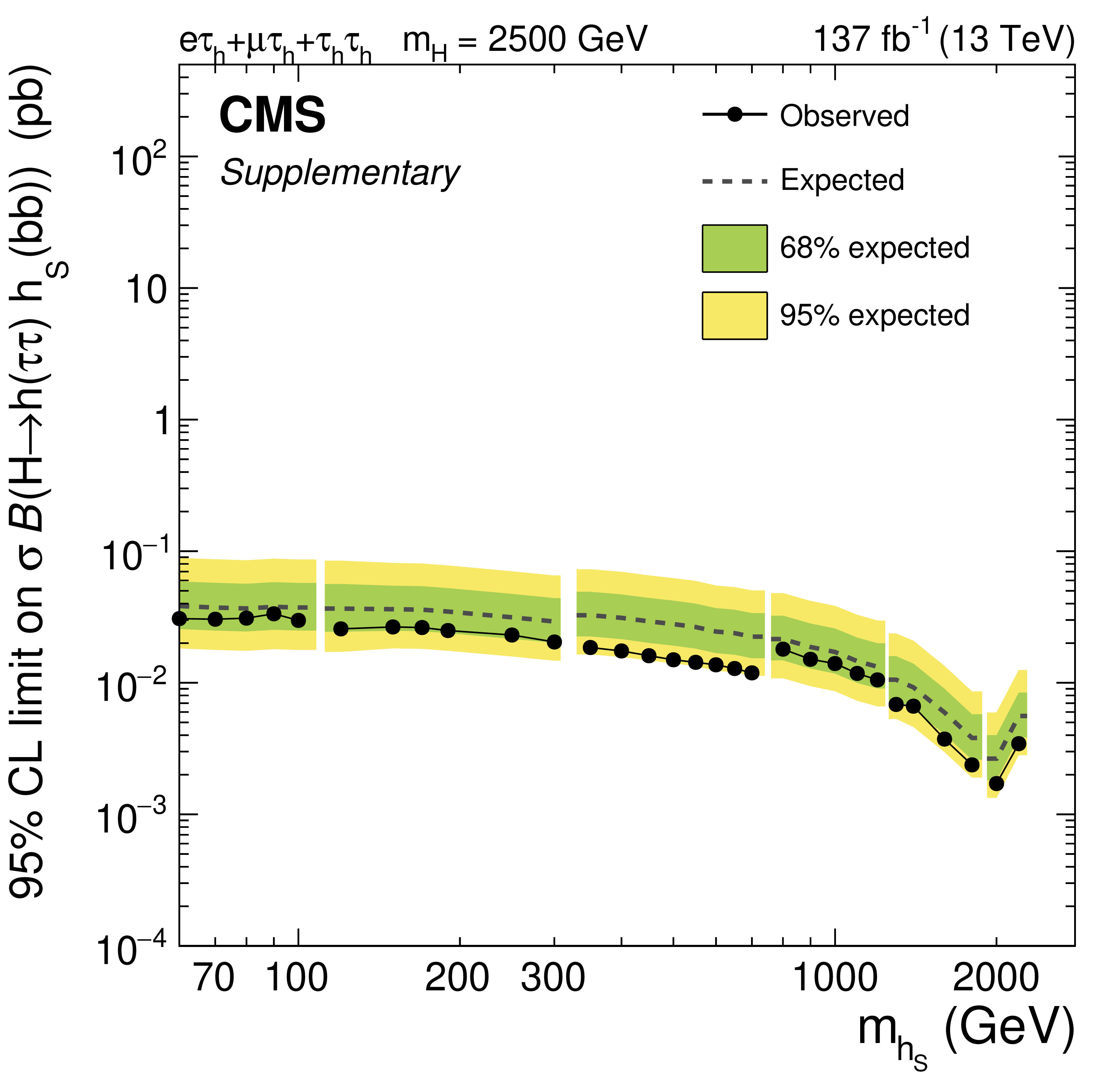
Expected and observed 95% confidence level upper limits on $ {\sigma \,\mathcal {B}({\mathrm {H}} \to {\mathrm {h}} ({\tau} {\tau}) {{\mathrm {h}} _{\text {S}}} ({\mathrm {b}} {\mathrm {b}}))}$ for $ {m_{{\mathrm {H}}}} = $ 2500 GeV and 60 $\leq {m_{{{\mathrm {h}} _{\text {S}}}}}\leq $ 2200 GeV. |
png pdf |
Additional Figure 20:
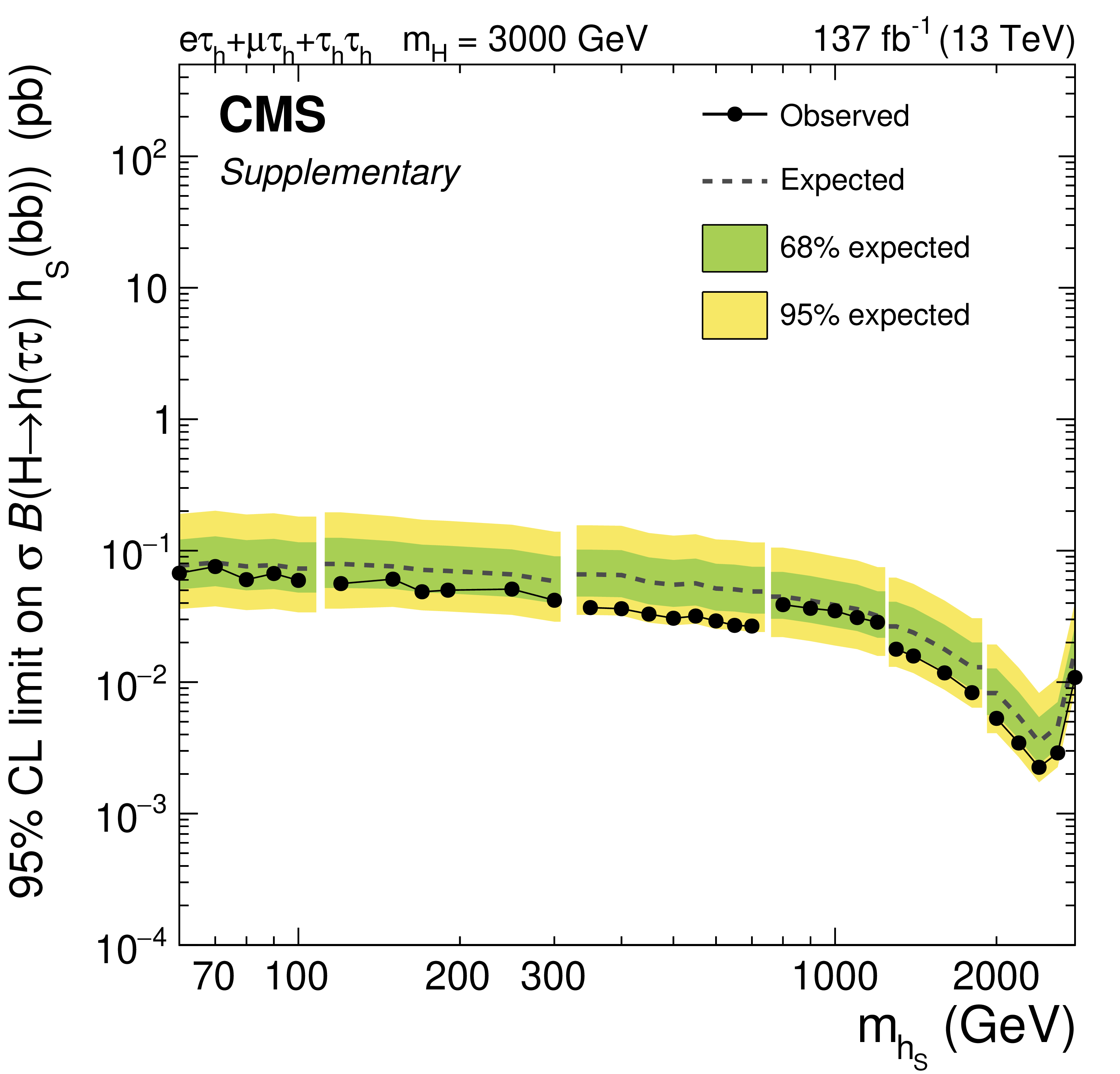
Expected and observed 95% confidence level upper limits on $ {\sigma \,\mathcal {B}({\mathrm {H}} \to {\mathrm {h}} ({\tau} {\tau}) {{\mathrm {h}} _{\text {S}}} ({\mathrm {b}} {\mathrm {b}}))}$ for $ {m_{{\mathrm {H}}}} = $ 3000 GeV and 60 $\leq {m_{{{\mathrm {h}} _{\text {S}}}}}\leq $ 2800 GeV. |
png pdf |
Additional Figure 21:
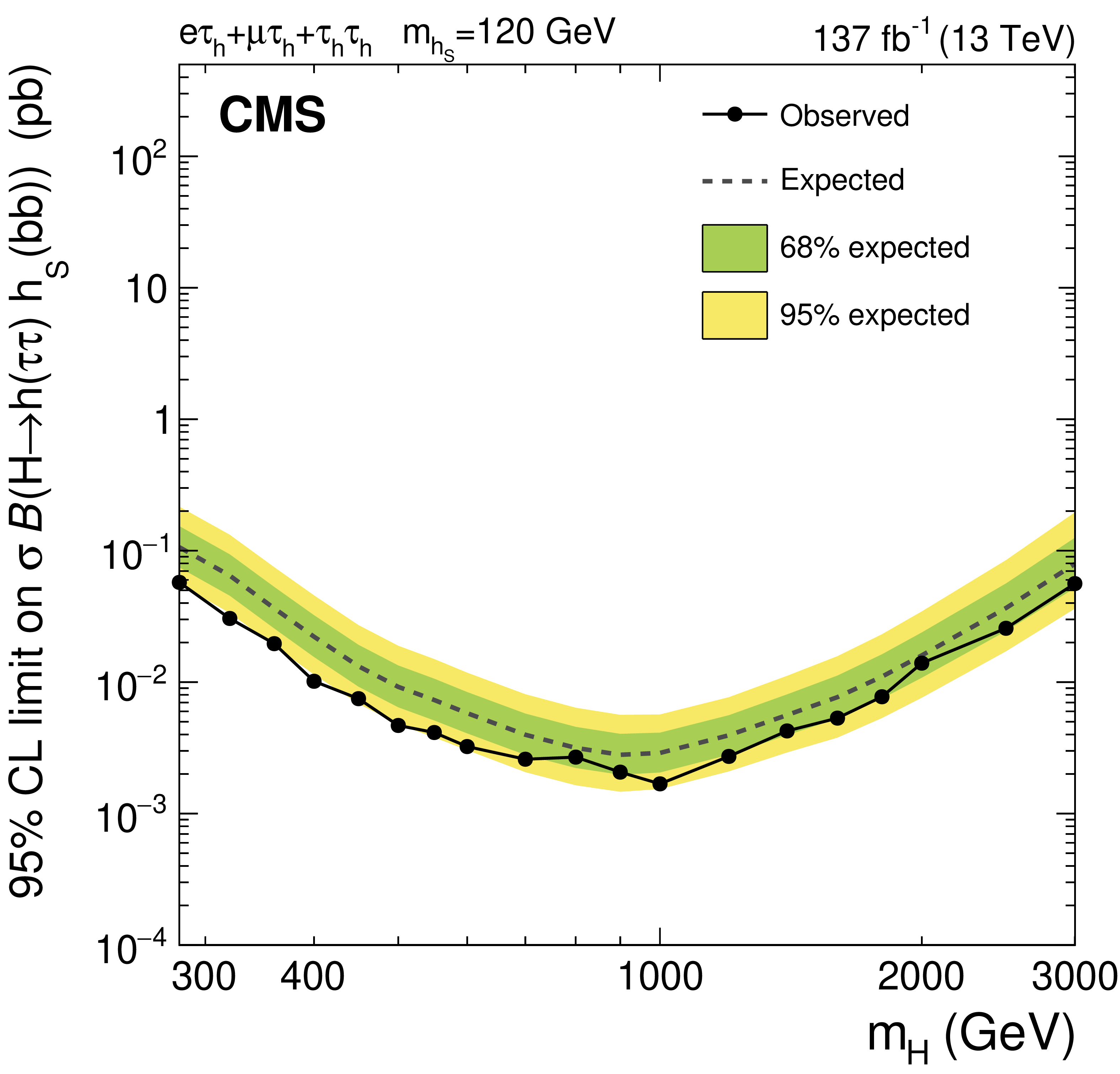
Expected and observed 95% confidence level upper limits on $ {\sigma \,\mathcal {B}({\mathrm {H}} \to {\mathrm {h}} ({\tau} {\tau}) {{\mathrm {h}} _{\text {S}}} ({\mathrm {b}} {\mathrm {b}}))}$ for $ {m_{{{\mathrm {h}} _{\text {S}}}}} = $ 120 GeV and $280\leq {m_{{\mathrm {H}}}}\leq $ 3000 GeV. |

png pdf |
Additional Figure 22:
Summary of the observed limits on $ {\sigma \,\mathcal {B}({\mathrm {H}} \to {\mathrm {h}} ({\tau} {\tau}) {{\mathrm {h}} _{\text {S}}} ({\mathrm {b}} {\mathrm {b}}))}$ for all tested pairs of $ {m_{{\mathrm {H}}}}$ and $ {m_{{{\mathrm {h}} _{\text {S}}}}}$. The limits are given by the color code of the figure. The region in the plane spanned by $ {m_{{\mathrm {H}}}}$ and $ {m_{{{\mathrm {h}} _{\text {S}}}}}$ where the observed limits fall below the maximally allowed values on $ {\sigma \,\mathcal {B}({\mathrm {H}} \to {\mathrm {h}} ({\tau} {\tau}) {{\mathrm {h}} _{\text {S}}} ({\mathrm {b}} {\mathrm {b}}))}$ in the context of the NMSSM, as provided by the LHC Higgs Working Group, are indicated by a red hatched area. |
png pdf |
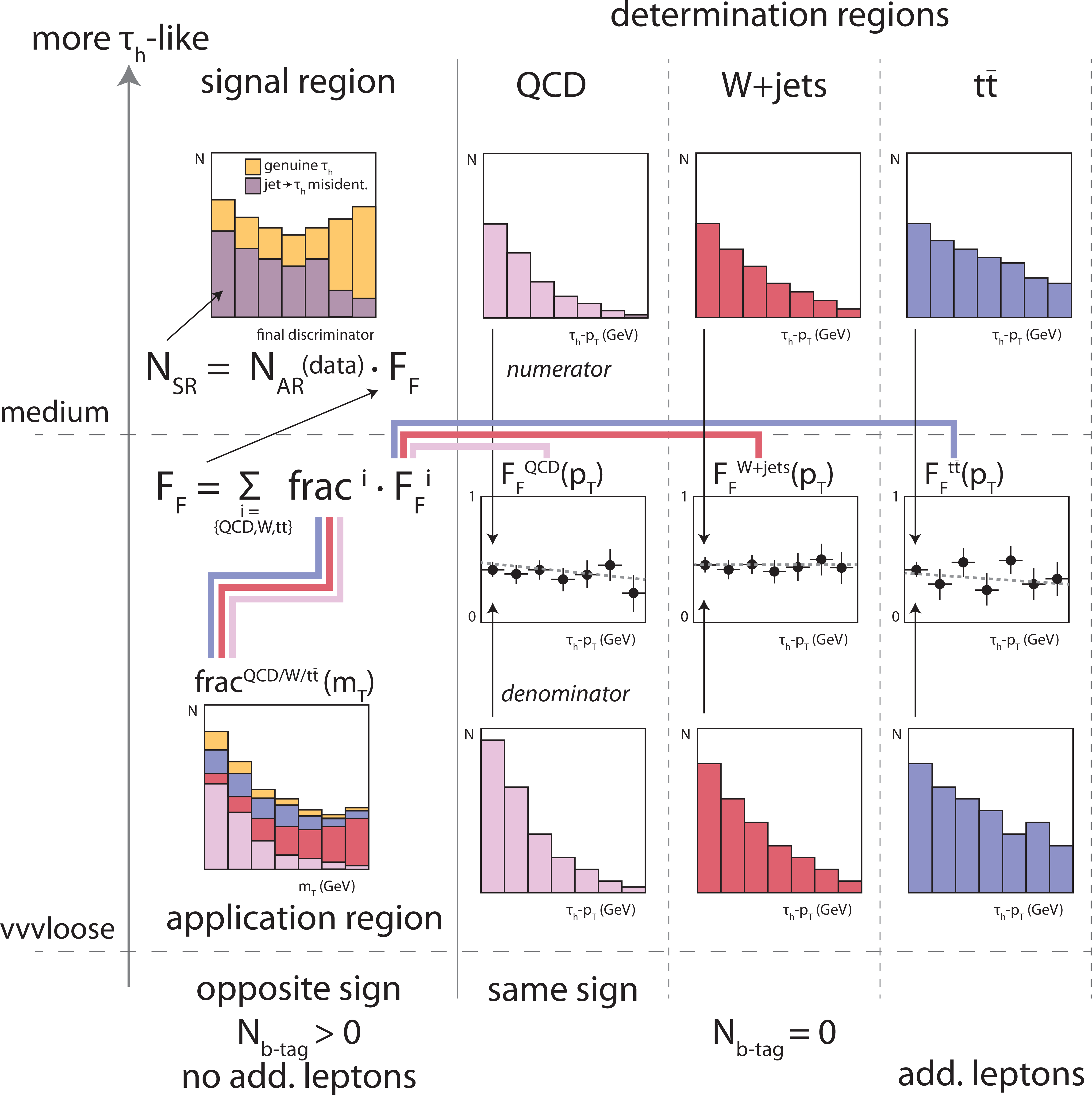
Additional Figure 23:
Schematic view of the $ {F_{\text {F}}}$-method used to estimate the $ {\text {jet}\to {\tau}_{\text {h}}}$ background from data. |
png pdf |
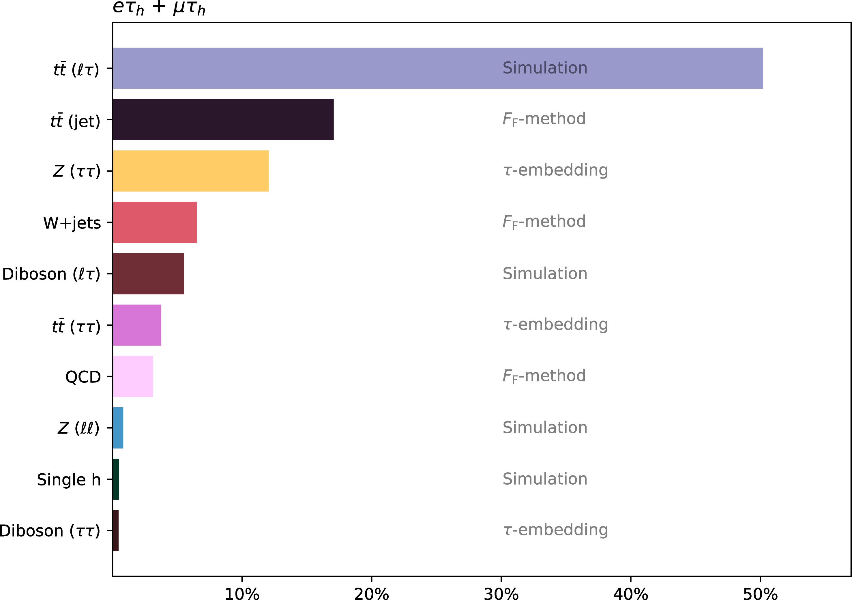
Additional Figure 24:
Expected event composition after selection, and different estimation methods used for background modelling in the $ {\mathrm {e}} {\tau}_{\text {h}} $ and $ {{\mu}} {\tau}_{\text {h}} $ final states. |

png pdf |
Additional Figure 25:
Expected event composition after selection, and different estimation methods used for background modelling in the $ {\tau}_{\text {h}} {\tau}_{\text {h}} $ final state. |
png pdf |
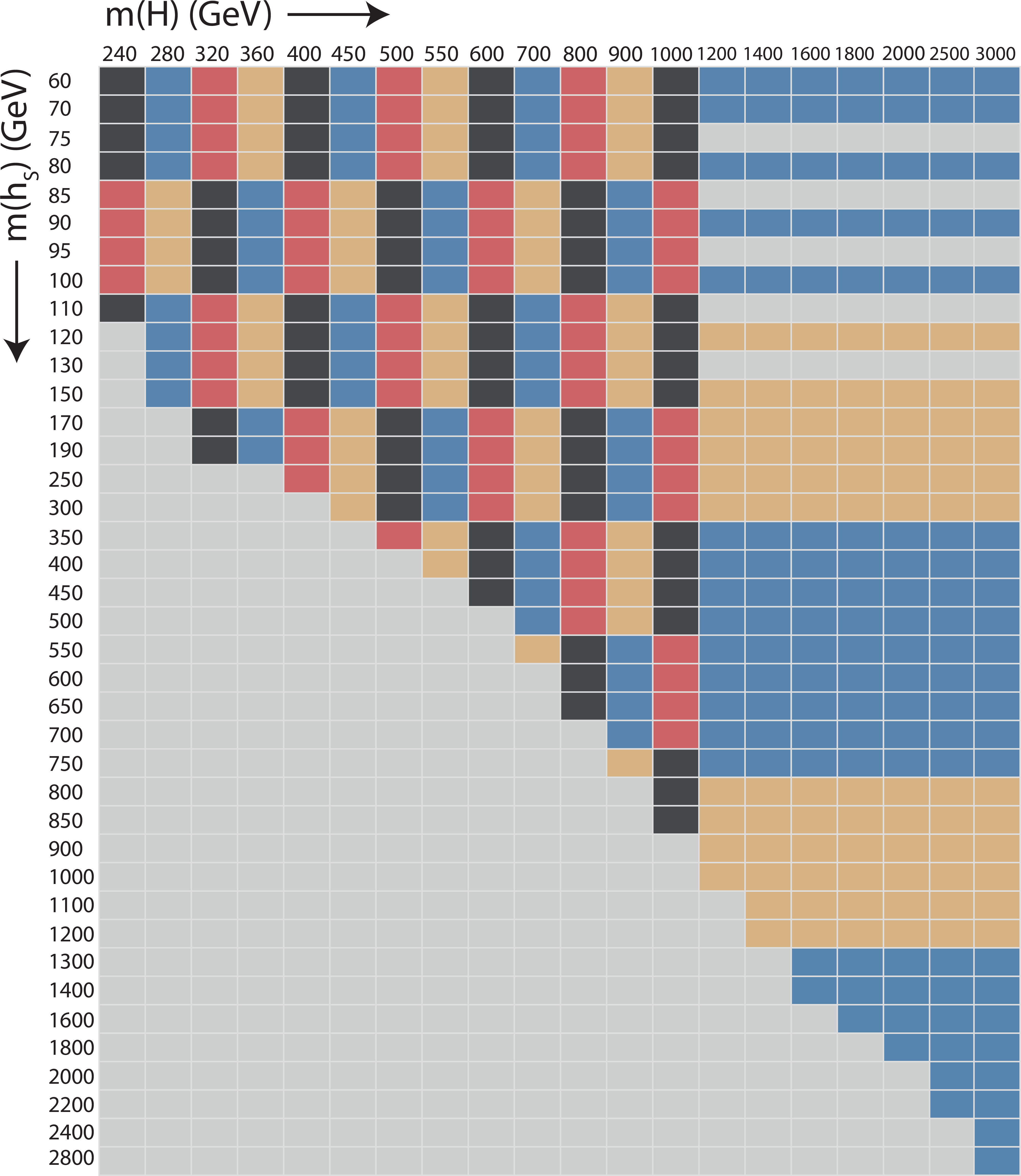
Additional Figure 26:
Grouping of simulated signal samples for the NN training used to classify signal and background events for the statistical inference of the signal. The used values for $ {m_{{\mathrm {H}}}}$ are given on the x-axis, the used values for $ {m_{{{\mathrm {h}} _{\text {S}}}}}$ on the y-axis of the figure. |
png pdf |
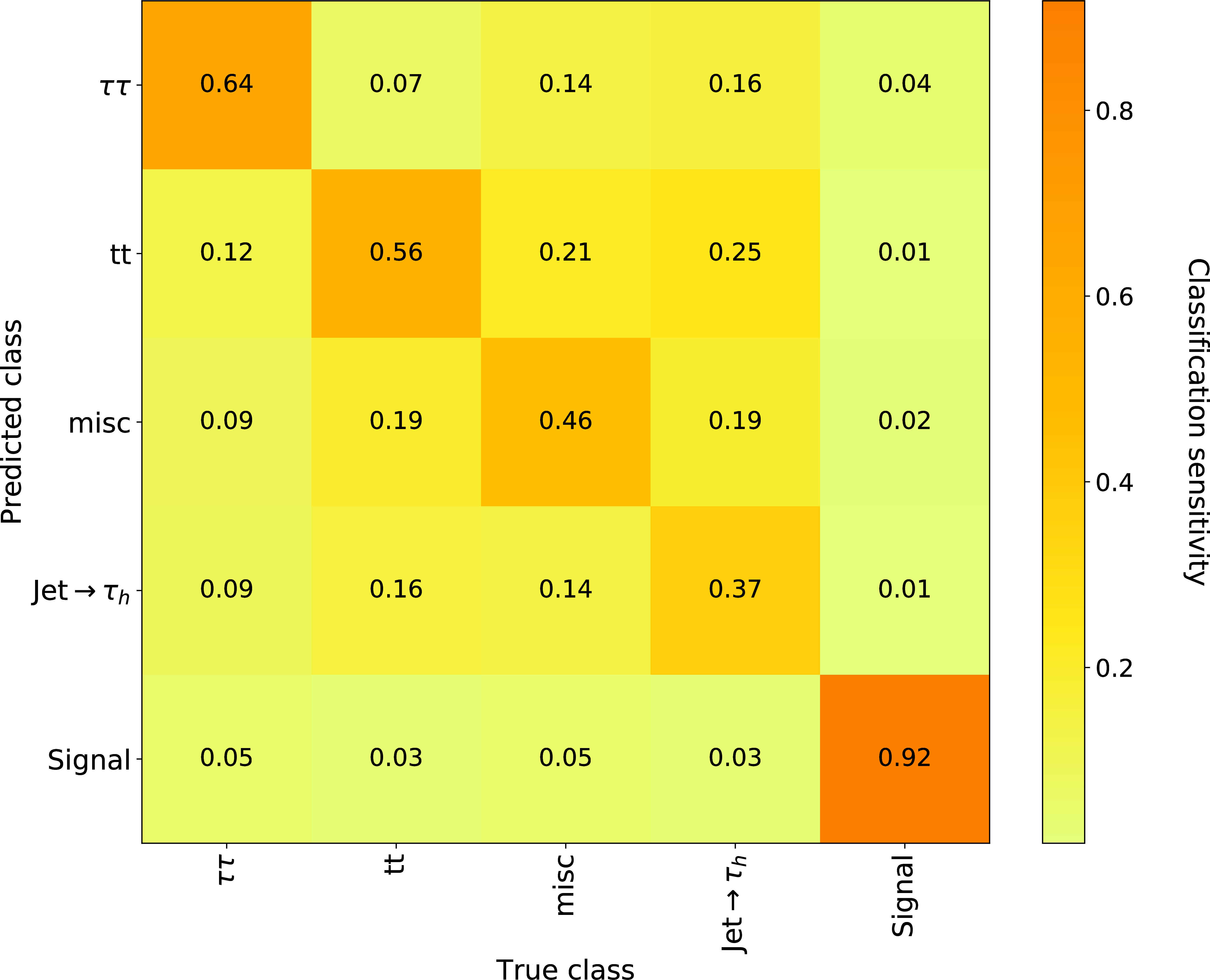
Additional Figure 27:
Confusion matrix of the NN training for $ {m_{{\mathrm {H}}}} = $ 500 GeV and 110 $ \leq {m_{{{\mathrm {h}} _{\text {S}}}}}\leq $ 150 GeV in the $ {{\mu}} {\tau}_{\text {h}} $ final state evaluated on the test data set used for the statistical inference of the signal in the 2018 data. The true event classes are given on the x-axis of the figure. The event classes predicted by the NN are given on the y-axis. In this representation all columns of the matrix have been normalized to $1$, corresponding to the classification sensitivity of the NN to each corresponding true event class. |

png pdf |
Additional Figure 28:
Confusion matrix of the NN training for $ {m_{{\mathrm {H}}}} = $ 500 GeV and 110 $ \leq {m_{{{\mathrm {h}} _{\text {S}}}}}\leq $ 150 GeV in the $ {{\mu}} {\tau}_{\text {h}} $ final state evaluated on the test data set used for the statistical inference of the signal in the 2018 data. The true event classes are given on the x-axis of the figure. The event classes predicted by the NN are given on the y-axis. In this representation all rows of the matrix have been normalized to $1$, corresponding to the classification purity of the NN to each corresponding true event class. Note that for the evaluation of the confusion matrix all true event classes enter with the same weight. |
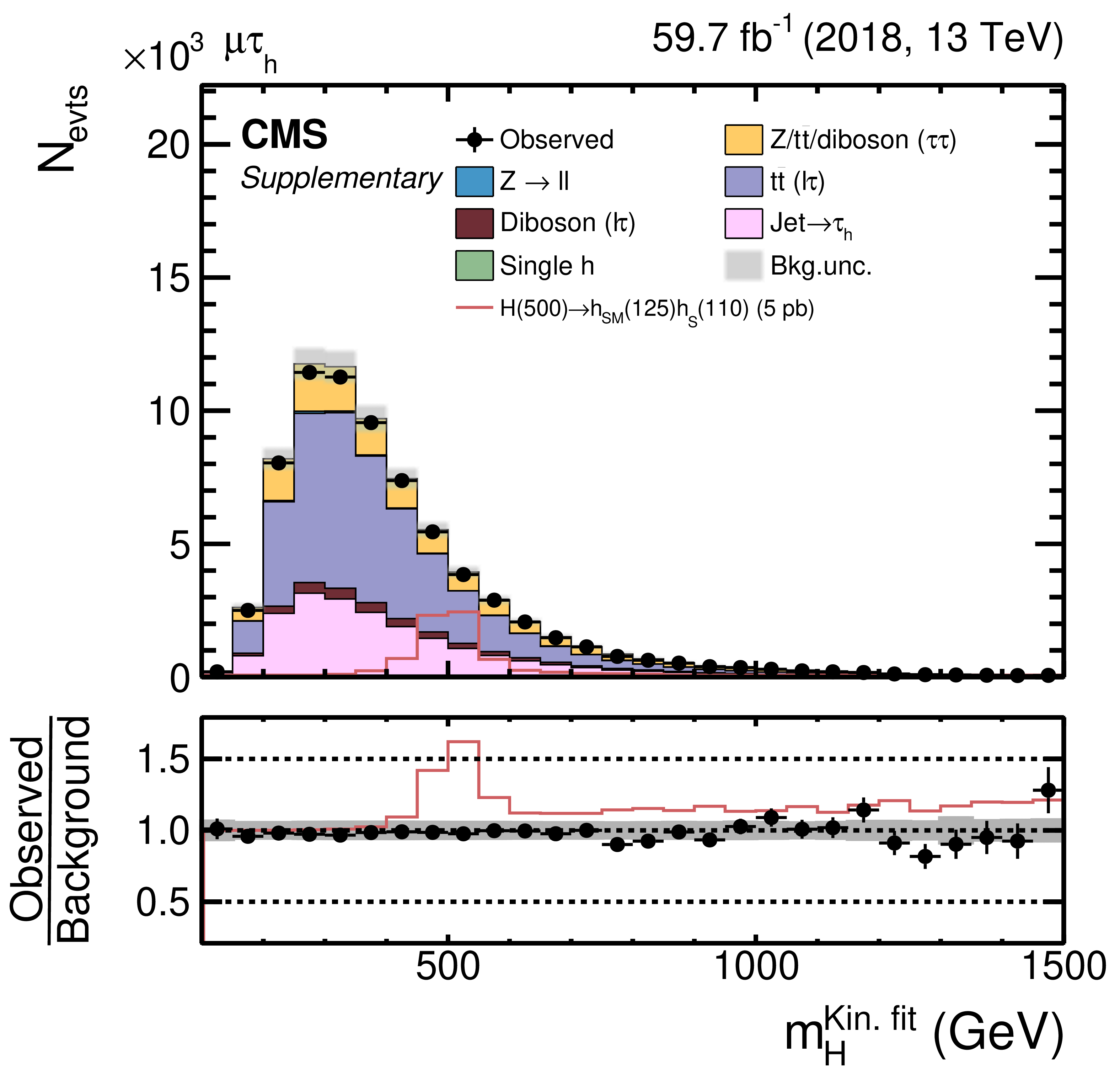
png pdf |
Additional Figure 29:
Estimate of $ {m_{{\mathrm {H}}}}$ from the kinematic fit as discussed in the text, as input to the event multi-classification. The model for the 2018 data in the $ {{\mu}} {\tau}_{\text {h}} $ final state is shown before any fit to the data. The shaded band corresponds to the combined statistical and systematic uncertainties of the background estimation. |

png pdf |
Additional Figure 30:
Estimate of $ {m_{{{\mathrm {h}} _{\text {S}}}}}$ from the kinematic fit as discussed in the text, as input to the event multi-classification. The model for the 2018 data in the $ {{\mu}} {\tau}_{\text {h}} $ final state is shown before any fit to the data. The shaded band corresponds to the combined statistical and systematic uncertainties of the background estimation. |
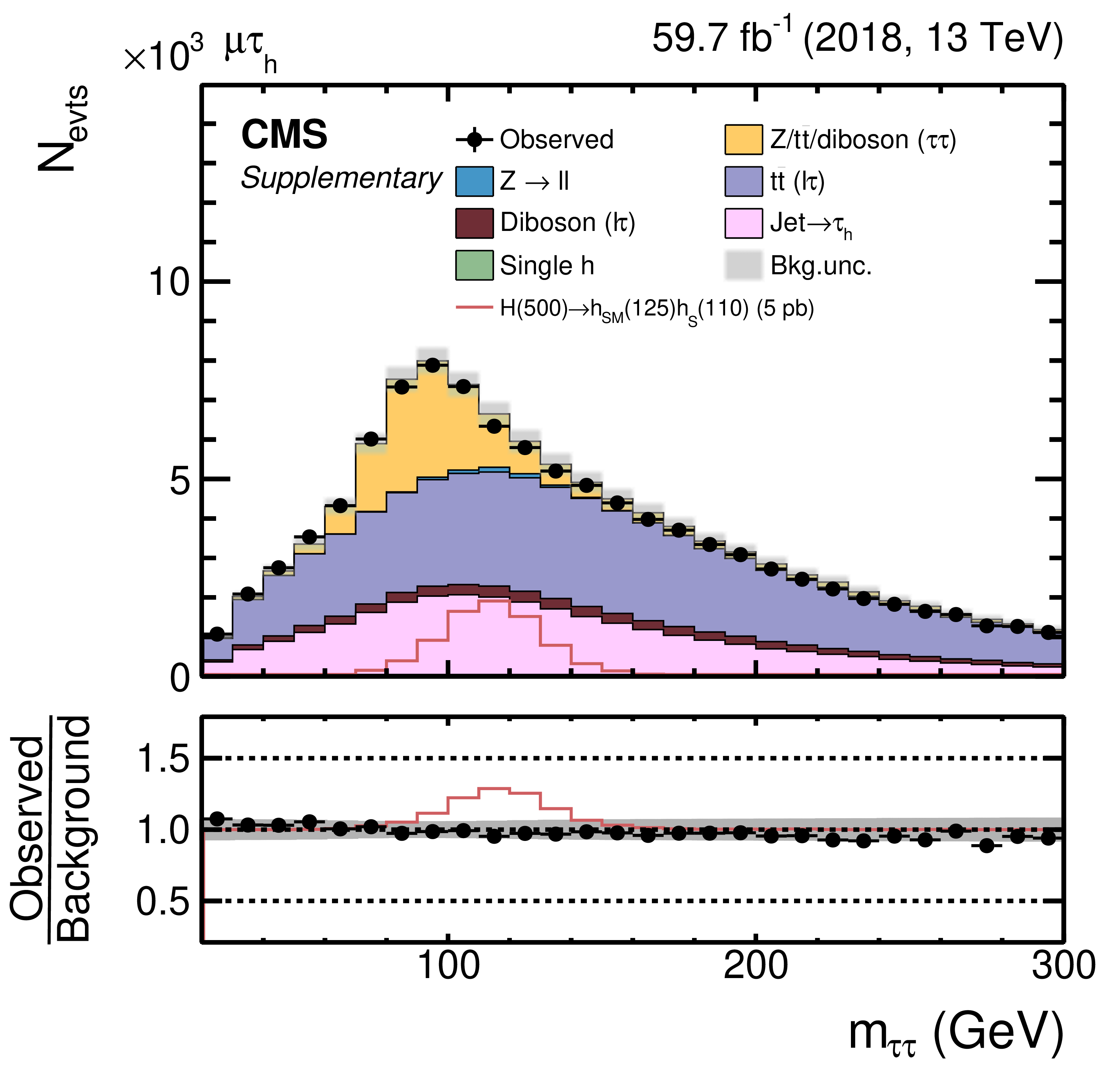
png pdf |
Additional Figure 31:
Estimate of $ {m_{{\tau} {\tau}}} $ as discussed in the text, as input to the event multi-classification. The model for the 2018 data in the $ {{\mu}} {\tau}_{\text {h}} $ final state is shown before any fit to the data. The shaded band corresponds to the combined statistical and systematic uncertainties of the background estimation. |

png pdf |
Additional Figure 32:
Mass of the visible $ {\tau} {\tau}$ system $ {m_{\text {vis}}} $, as input to the event multi-classification. The model for the 2018 data in the $ {{\mu}} {\tau}_{\text {h}} $ final state is shown before any fit to the data. The shaded band corresponds to the combined statistical and systematic uncertainties of the background estimation. |
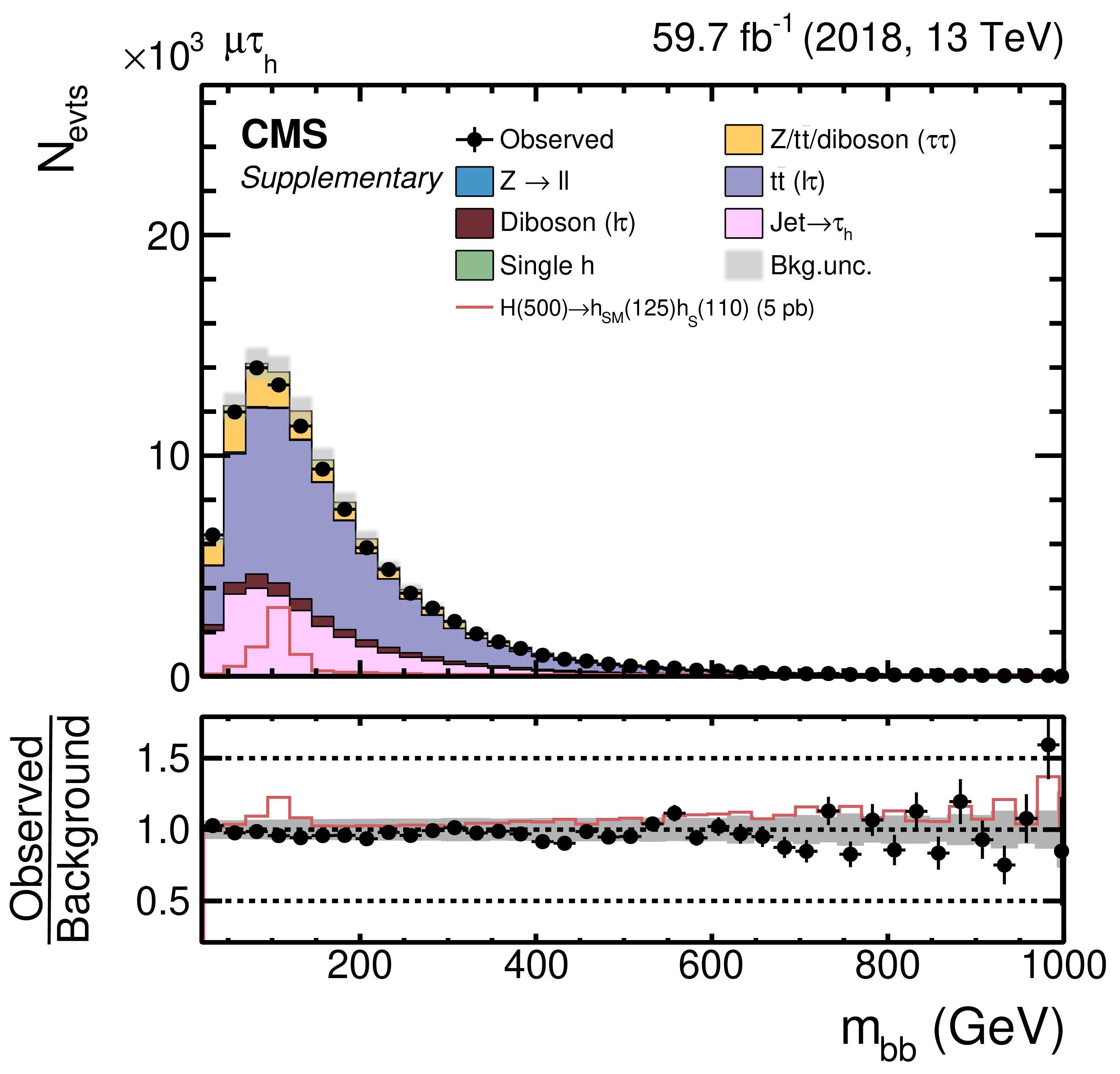
png pdf |
Additional Figure 33:
Mass of the $ {\mathrm {b}} {\mathrm {b}} $ system $m_{{\mathrm {b}} {\mathrm {b}}}$, as input to the event multi-classification. The model for the 2018 data in the $ {{\mu}} {\tau}_{\text {h}} $ final state is shown before any fit to the data. The shaded band corresponds to the combined statistical and systematic uncertainties of the background estimation. |
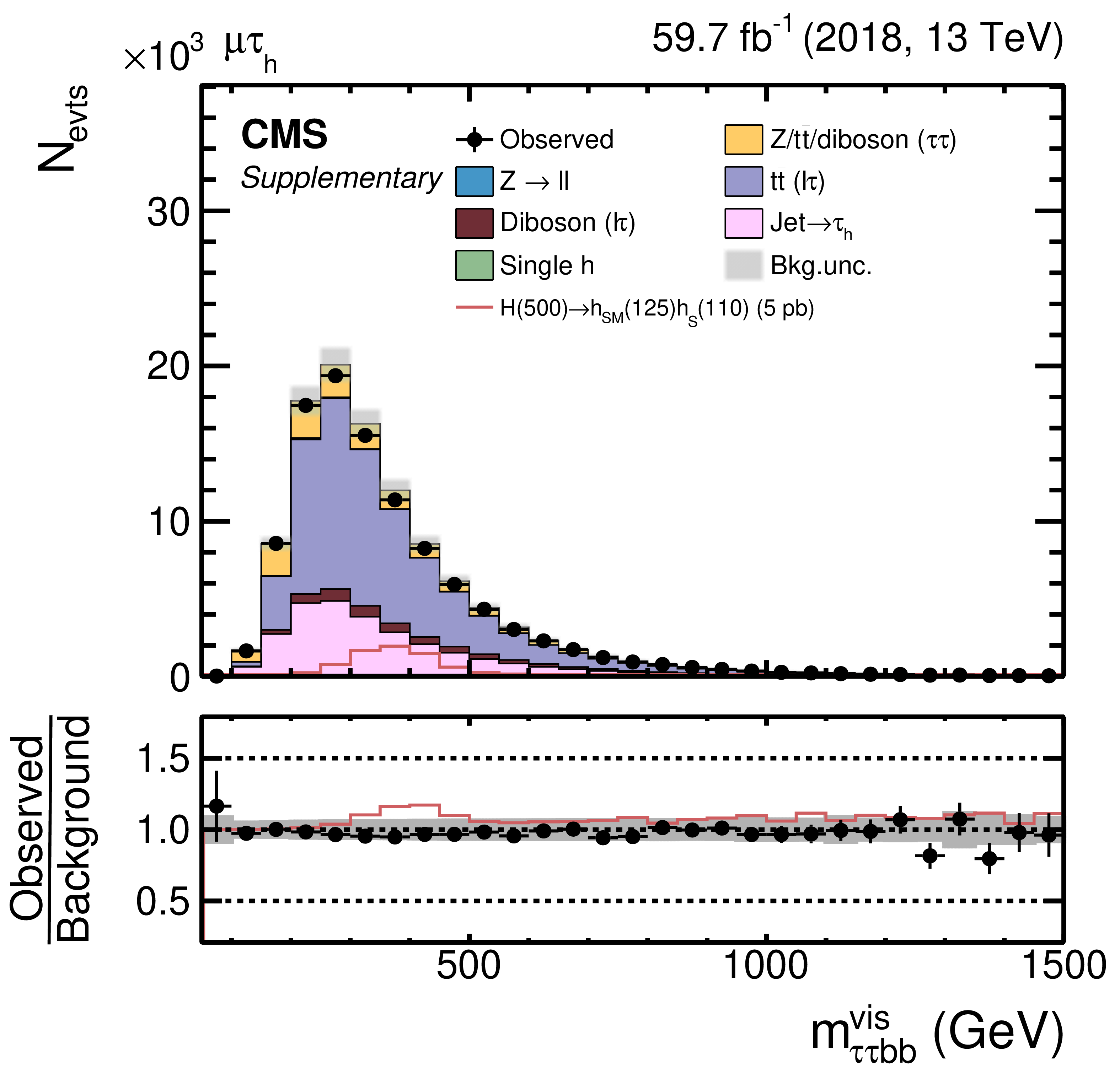
png pdf |
Additional Figure 34:
Mass of the visible $ {\tau} {\tau} {\mathrm {b}} {\mathrm {b}} $ system $m_{{\tau} {\tau} {\mathrm {b}} {\mathrm {b}}}^{\text {vis}}$, as input to the event multi-classification. The model for the 2018 data in the $ {{\mu}} {\tau}_{\text {h}} $ final state is shown before any fit to the data. The shaded band corresponds to the combined statistical and systematic uncertainties of the background estimation. |
png pdf |
Additional Figure 35:
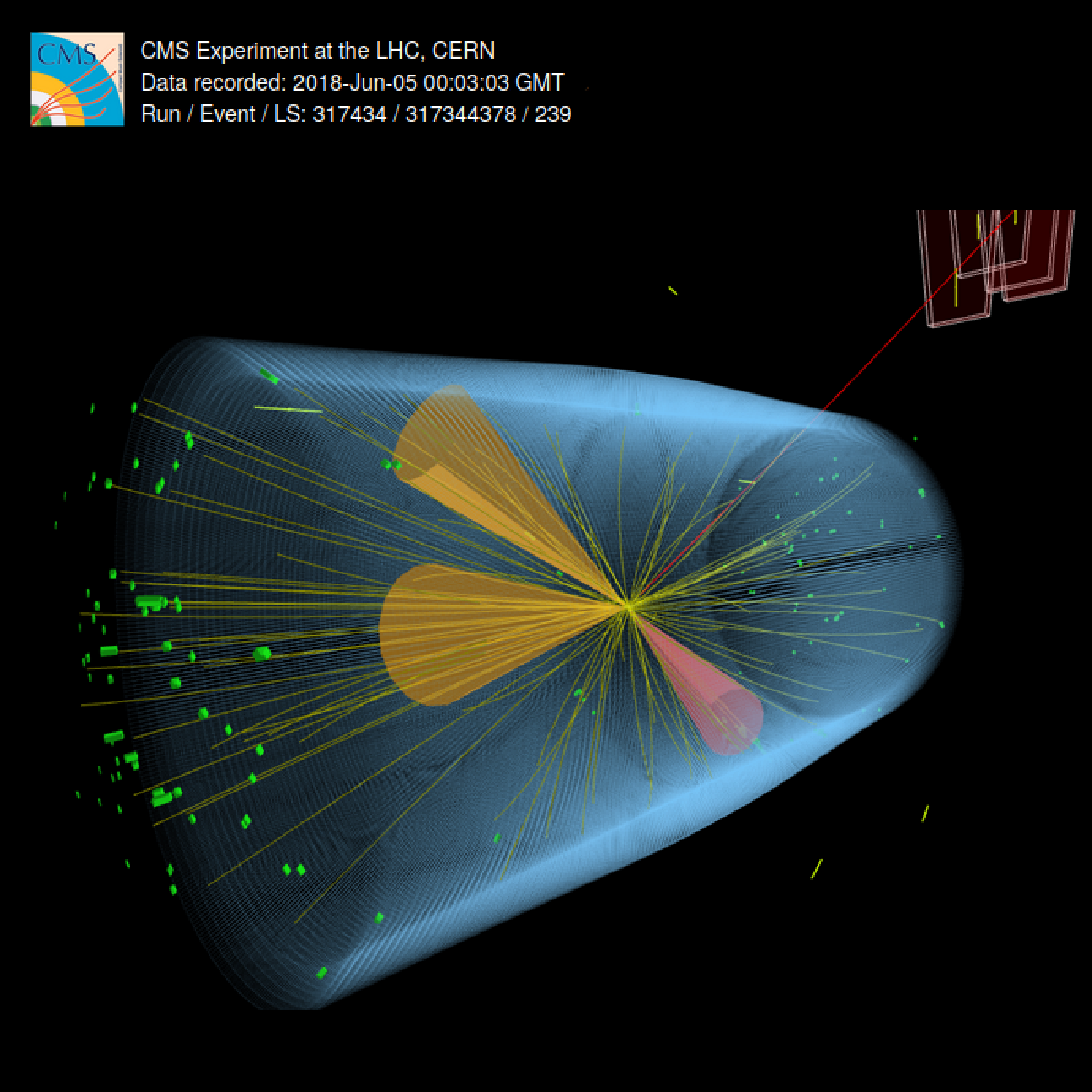
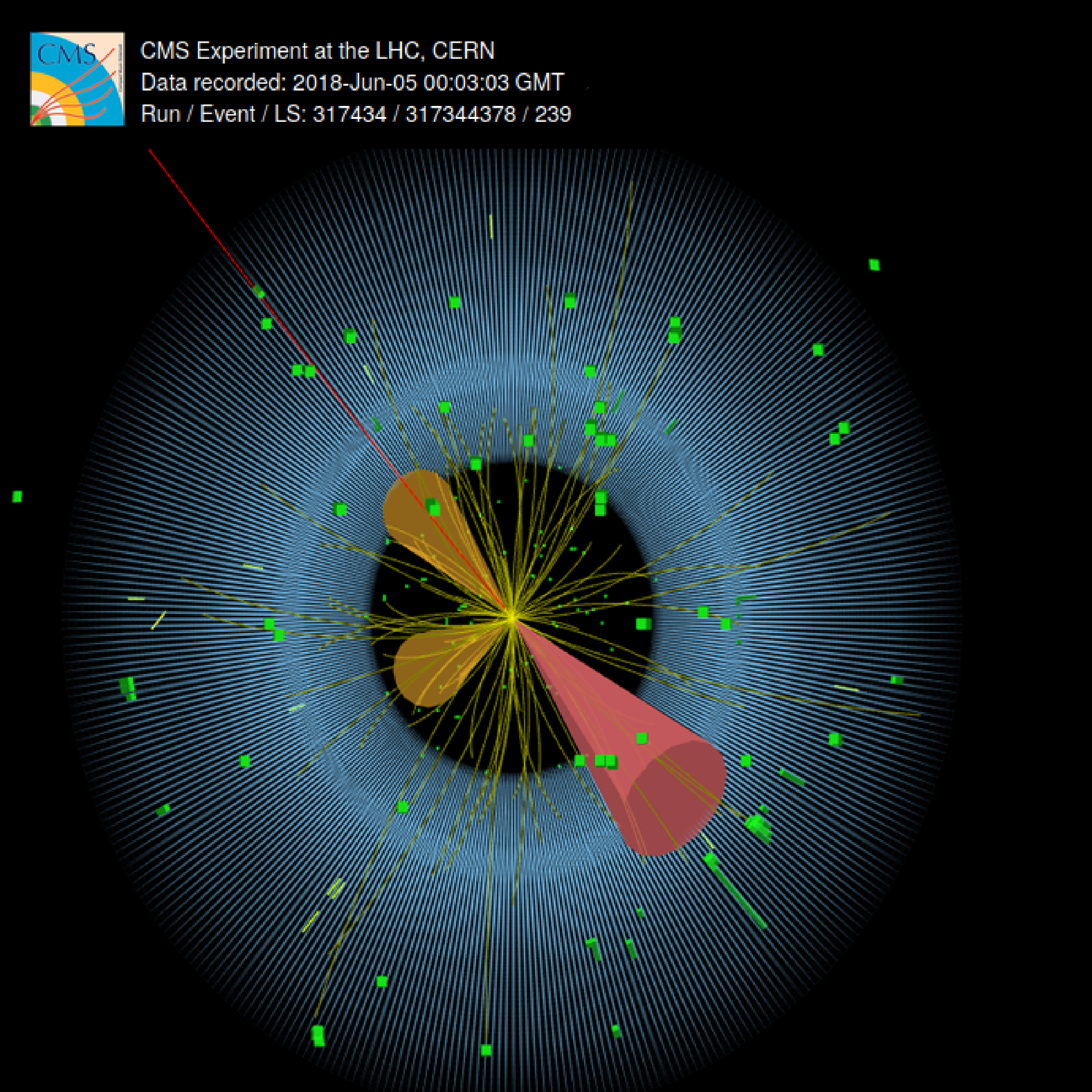
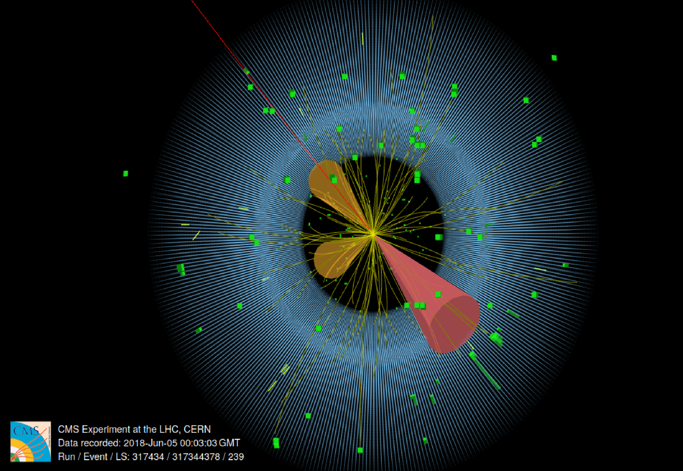
Display of an event with $y_{\text {Signal}}= $ 0.70 in the $ {{\mu}} {\tau}_{\text {h}} $ final state in the 2018 data set. In addition to the b jets, indicated by orange cones, a $ {{\mu}}$ (red line) and a $ {\tau}_{\text {h}} $ decay (red cone) are reconstructed. The same event is shown in different views (square versions of displays). |
png pdf |
Additional Figure 36:
Display of an event with $y_{\text {Signal}}= $ 0.70 in the $ {{\mu}} {\tau}_{\text {h}} $ final state in the 2018 data set. In addition to the b jets, indicated by orange cones, a $ {{\mu}}$ (red line) and a $ {\tau}_{\text {h}} $ decay (red cone) are reconstructed. The same event is shown in different views (square versions of displays). |
png pdf |
Additional Figure 37:
Display of an event with $y_{\text {Signal}}= $ 0.70 in the $ {{\mu}} {\tau}_{\text {h}} $ final state in the 2018 data set. In addition to the b jets, indicated by orange cones, a $ {{\mu}}$ (red line) and a $ {\tau}_{\text {h}} $ decay (red cone) are reconstructed. The same event is shown in different views (square versions of displays). |
png pdf |
Additional Figure 38:
Display of an event with $y_{\text {Signal}}= $ 0.70 in the $ {{\mu}} {\tau}_{\text {h}} $ final state in the 2018 data set. In addition to the b jets, indicated by orange cones, a $ {{\mu}}$ (red line) and a $ {\tau}_{\text {h}} $ decay (red cone) are reconstructed. The same event is shown in different views (square versions of displays). |

png pdf |
Additional Figure 39:
Display of an event with $y_{\text {Signal}}= $ 0.70 in the $ {{\mu}} {\tau}_{\text {h}} $ final state in the 2018 data set. In addition to the b jets, indicated by orange cones, a $ {{\mu}}$ (red line) and a $ {\tau}_{\text {h}} $ decay (red cone) are reconstructed. The same event is shown in different views (square versions of displays). |

png pdf |
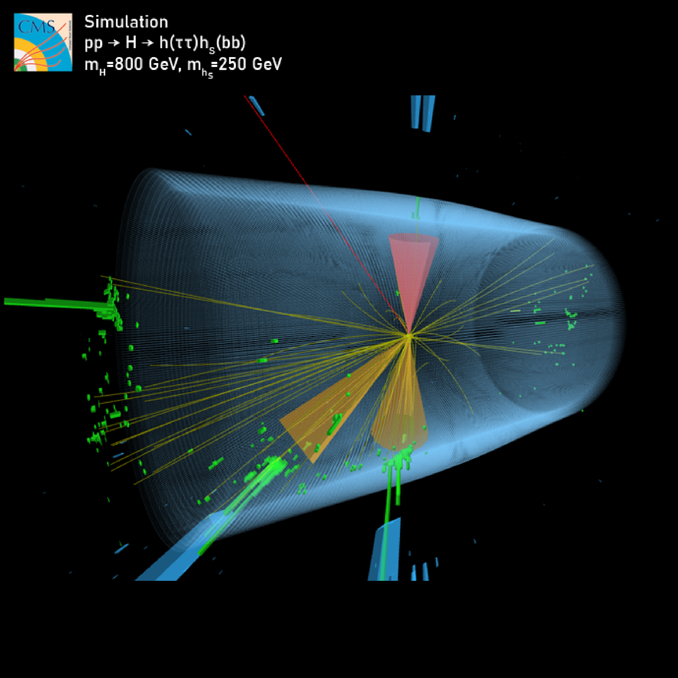
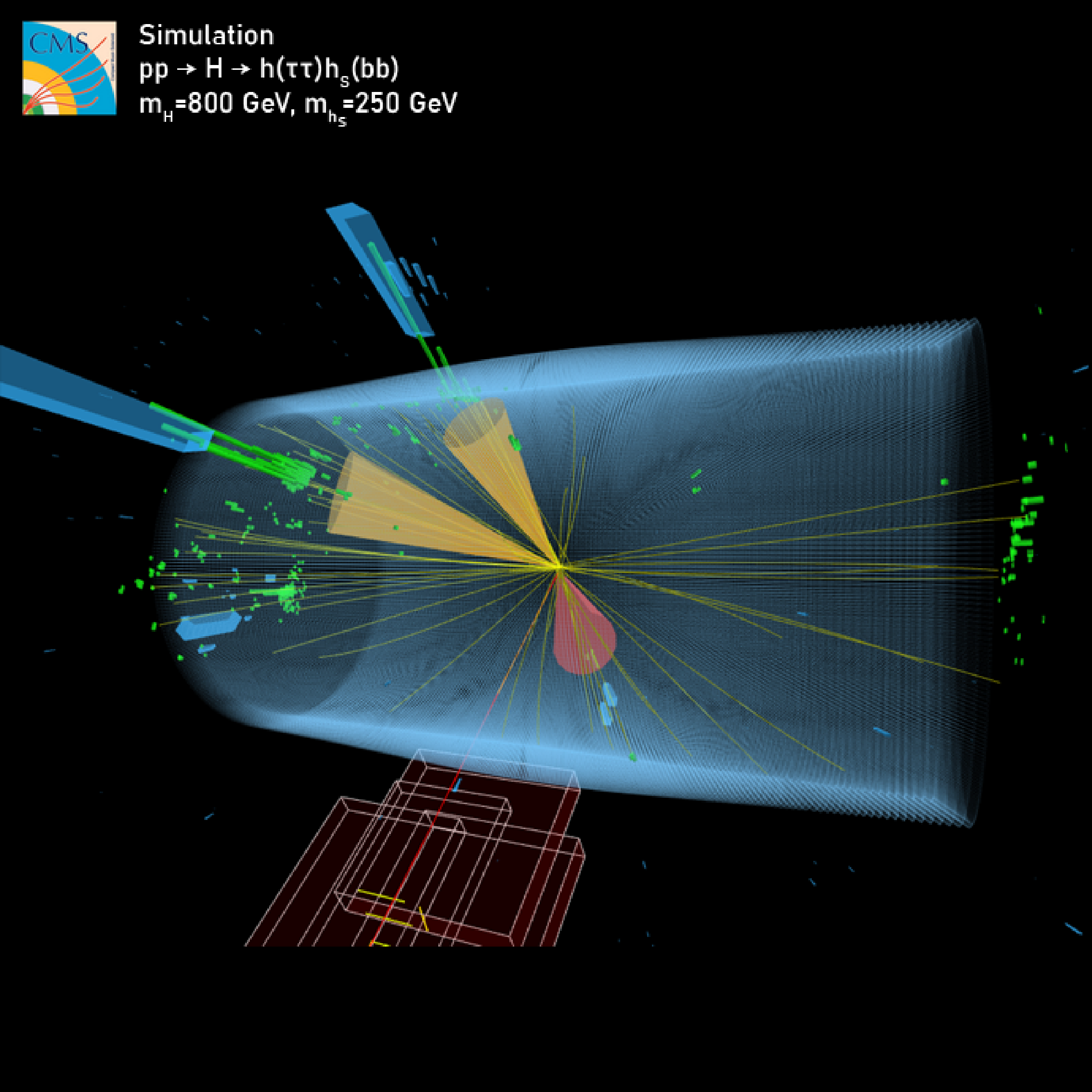
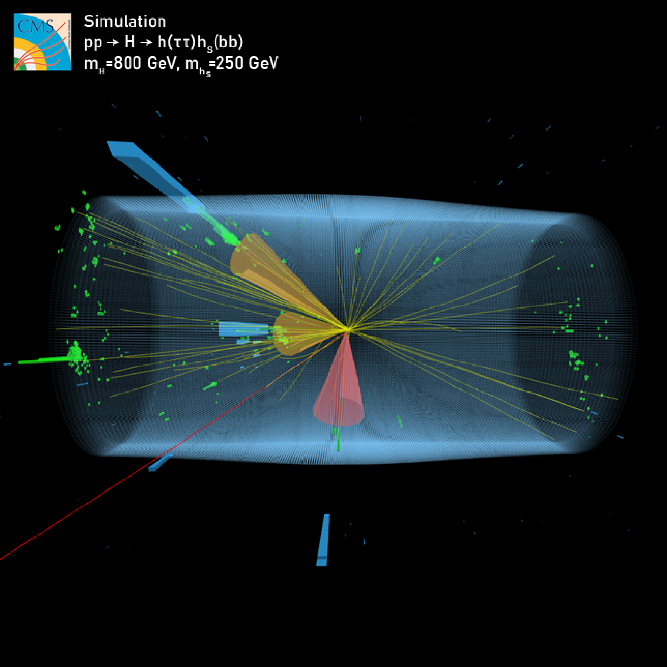
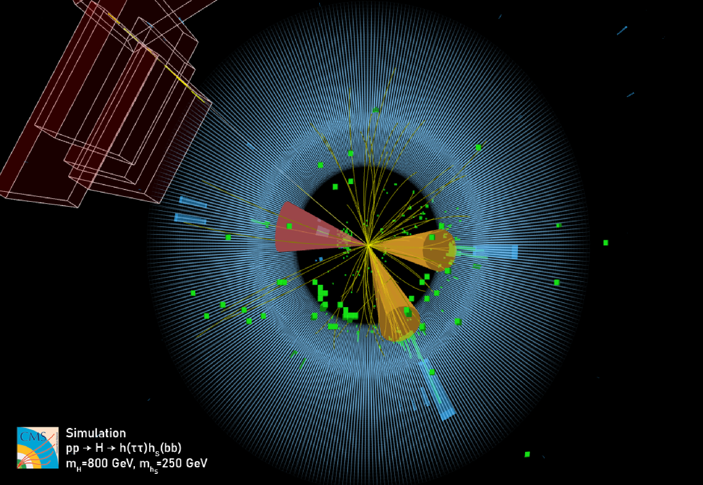
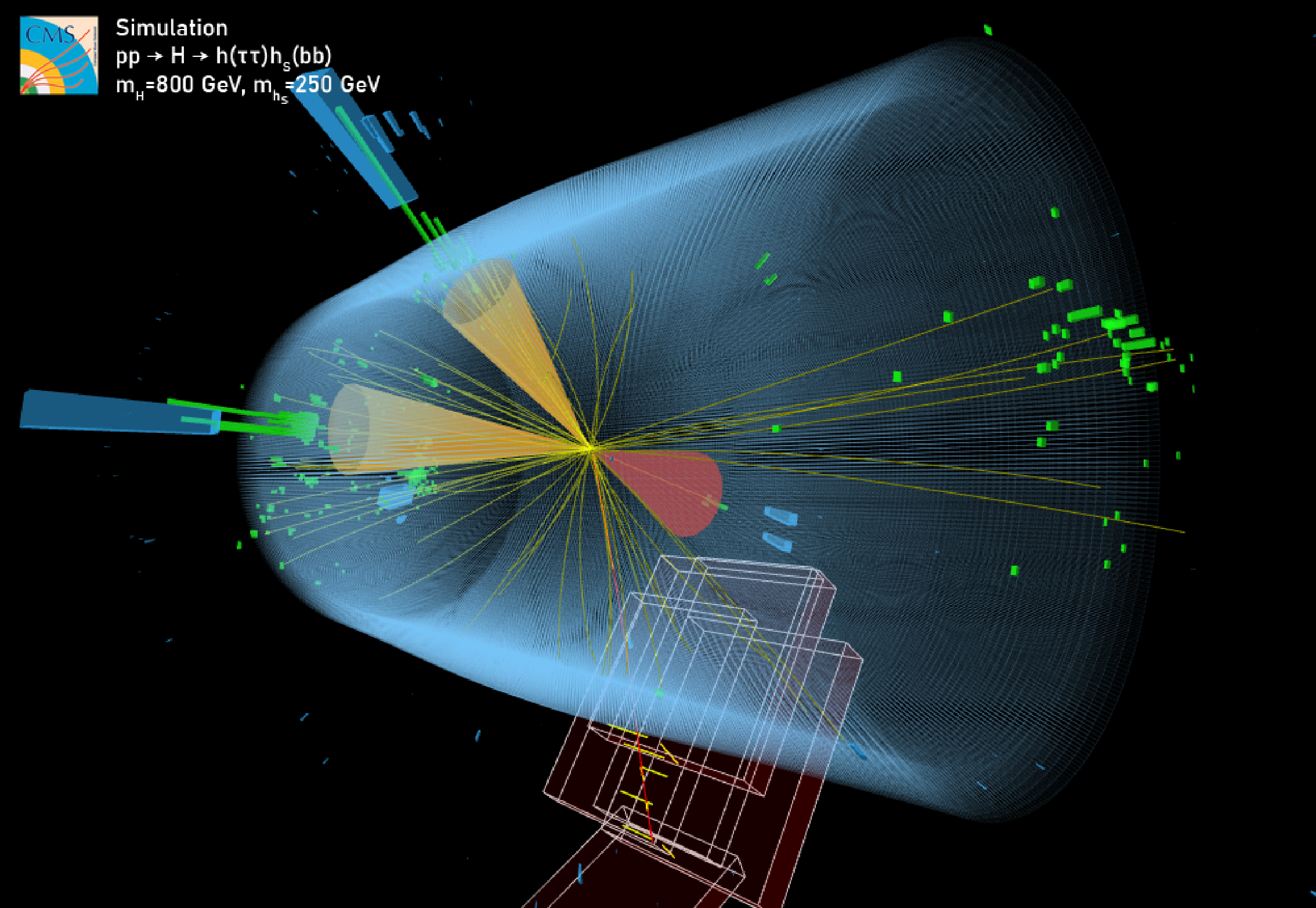
Additional Figure 40:
Display of a signal event with $ {m_{{\mathrm {H}}}} = $ 800 GeV and $ {m_{{{\mathrm {h}} _{\text {S}}}}} = $ 250 GeV in the $ {{\mu}} {\tau}_{\text {h}} $ final state from simulation. In addition to the b jets, indicated by orange cones, a $ {{\mu}}$ (red line) and a $ {\tau}_{\text {h}} $ decay (red cone) are reconstructed. The same event is shown in different views (square versions of displays). |
png pdf |
Additional Figure 41:
Display of a signal event with $ {m_{{\mathrm {H}}}} = $ 800 GeV and $ {m_{{{\mathrm {h}} _{\text {S}}}}} = $ 250 GeV in the $ {{\mu}} {\tau}_{\text {h}} $ final state from simulation. In addition to the b jets, indicated by orange cones, a $ {{\mu}}$ (red line) and a $ {\tau}_{\text {h}} $ decay (red cone) are reconstructed. The same event is shown in different views (square versions of displays). |
png pdf |
Additional Figure 42:
Display of a signal event with $ {m_{{\mathrm {H}}}} = $ 800 GeV and $ {m_{{{\mathrm {h}} _{\text {S}}}}} = $ 250 GeV in the $ {{\mu}} {\tau}_{\text {h}} $ final state from simulation. In addition to the b jets, indicated by orange cones, a $ {{\mu}}$ (red line) and a $ {\tau}_{\text {h}} $ decay (red cone) are reconstructed. The same event is shown in different views (square versions of displays). |

png pdf |
Additional Figure 43:
Display of a signal event with $ {m_{{\mathrm {H}}}} = $ 800 GeV and $ {m_{{{\mathrm {h}} _{\text {S}}}}} = $ 250 GeV in the $ {{\mu}} {\tau}_{\text {h}} $ final state from simulation. In addition to the b jets, indicated by orange cones, a $ {{\mu}}$ (red line) and a $ {\tau}_{\text {h}} $ decay (red cone) are reconstructed. The same event is shown in different views (square versions of displays). |

png pdf |
Additional Figure 44:
Display of a signal event with $ {m_{{\mathrm {H}}}} = $ 800 GeV and $ {m_{{{\mathrm {h}} _{\text {S}}}}} = $ 250 GeV in the $ {{\mu}} {\tau}_{\text {h}} $ final state from simulation. In addition to the b jets, indicated by orange cones, a $ {{\mu}}$ (red line) and a $ {\tau}_{\text {h}} $ decay (red cone) are reconstructed. The same event is shown in different views (square versions of displays). |
png pdf |
Additional Figure 45:
Display of a signal event with $ {m_{{\mathrm {H}}}} = $ 800 GeV and $ {m_{{{\mathrm {h}} _{\text {S}}}}} = $ 250 GeV in the $ {{\mu}} {\tau}_{\text {h}} $ final state from simulation. In addition to the b jets, indicated by orange cones, a $ {{\mu}}$ (red line) and a $ {\tau}_{\text {h}} $ decay (red cone) are reconstructed. The same event is shown in different views (square versions of displays). |
png pdf |
Additional Figure 46:
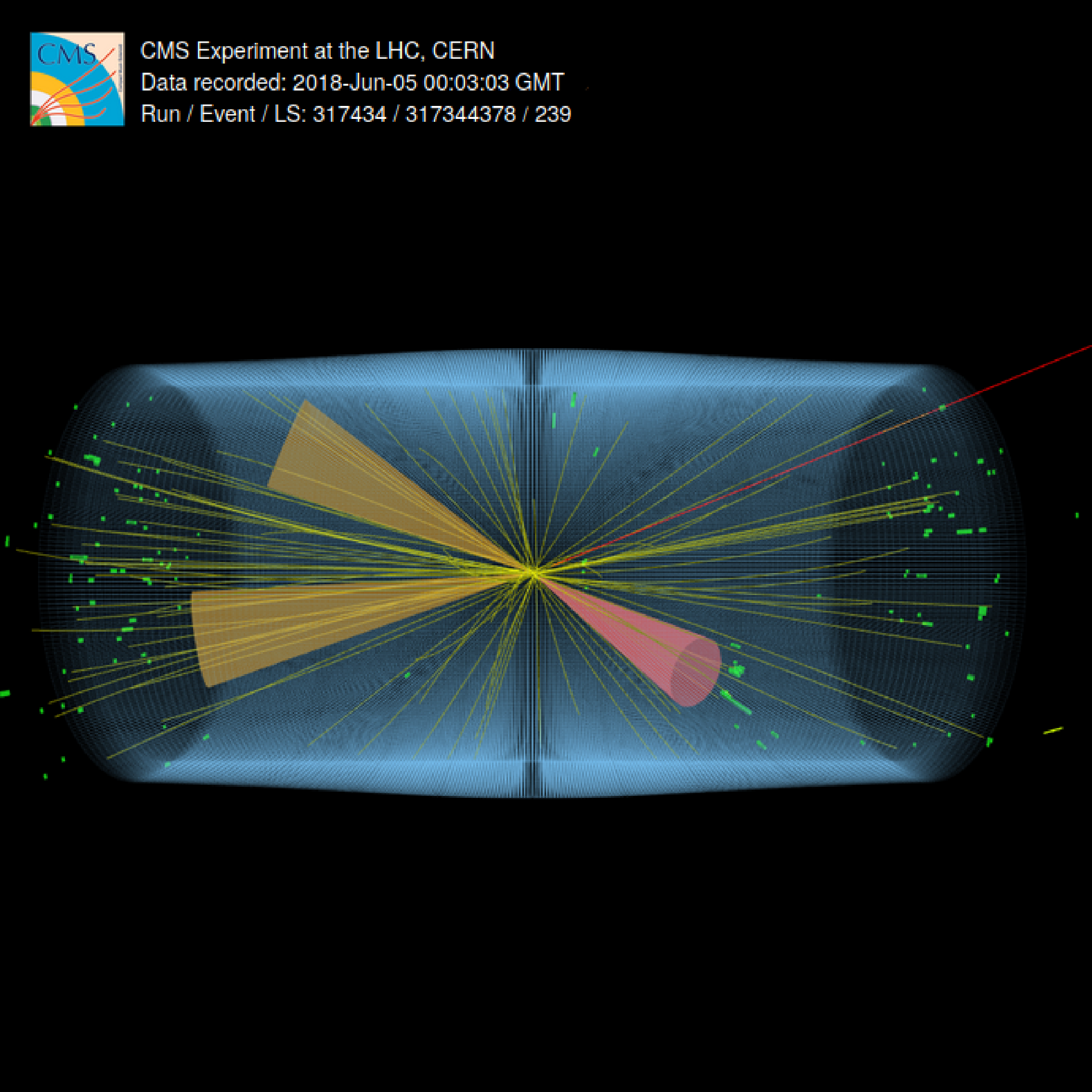
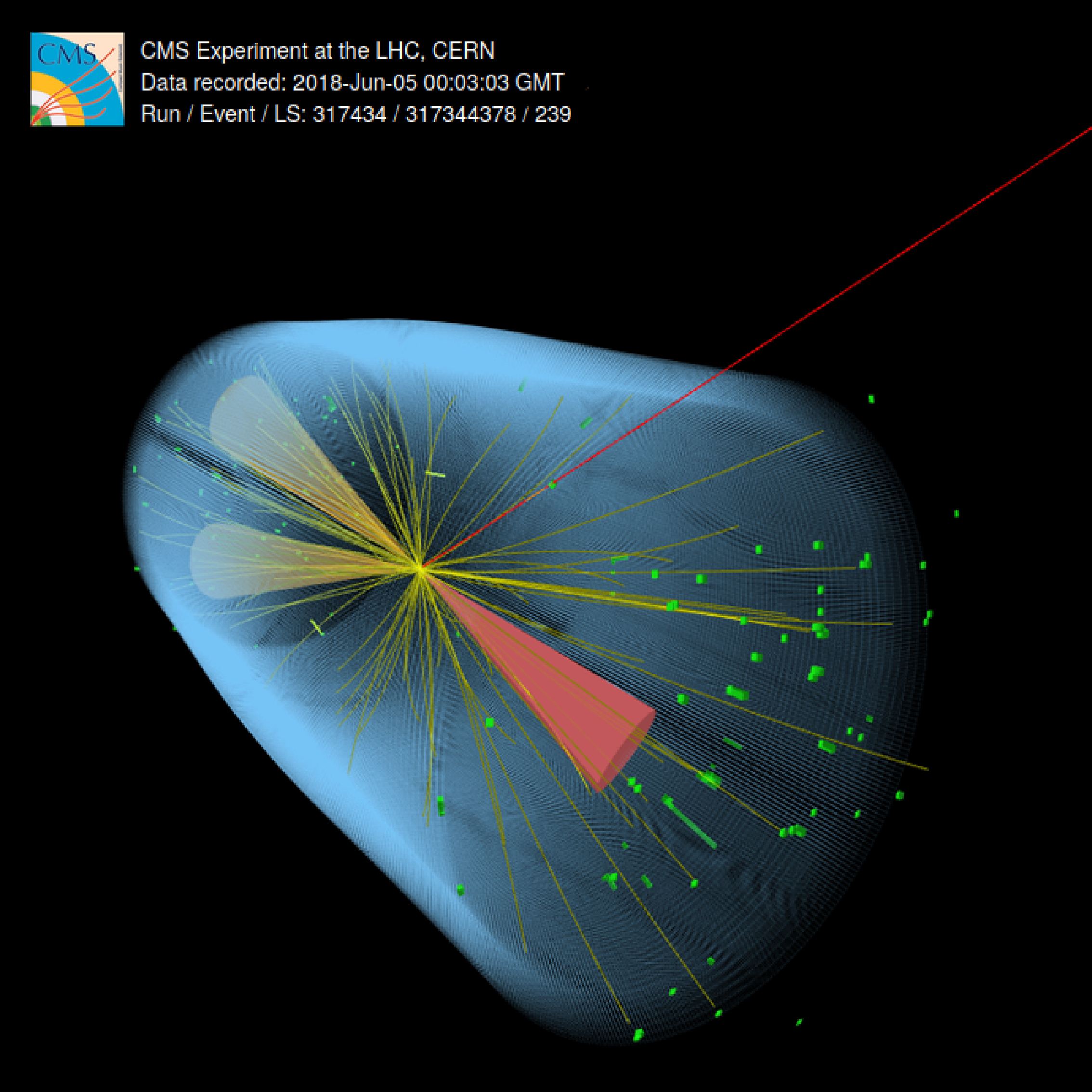
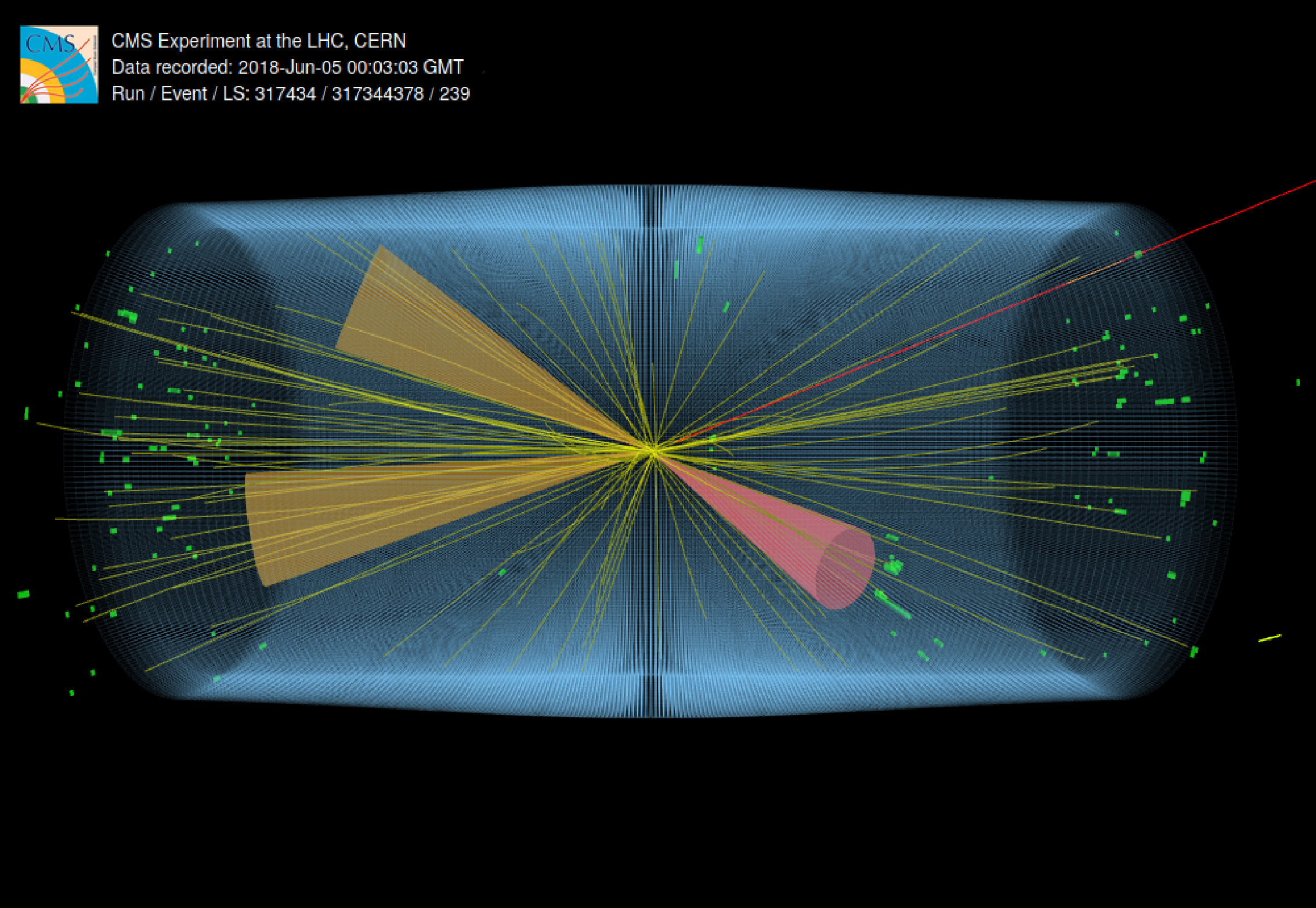
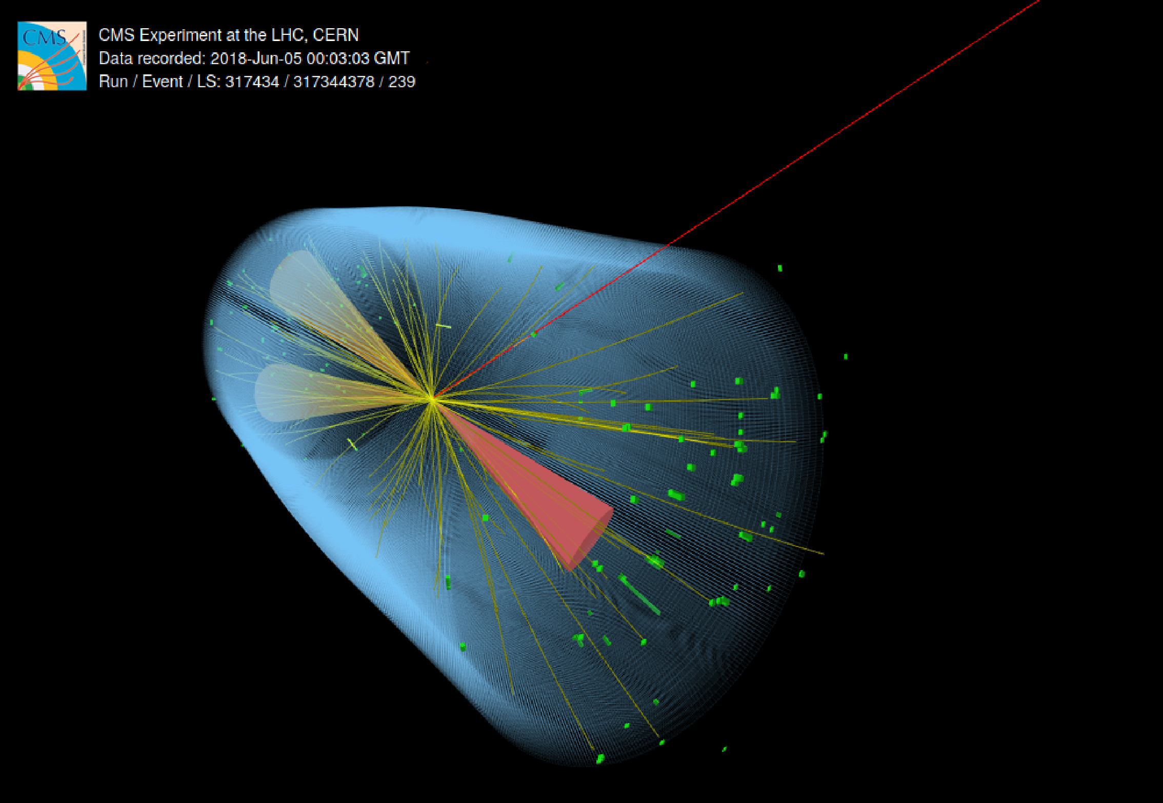
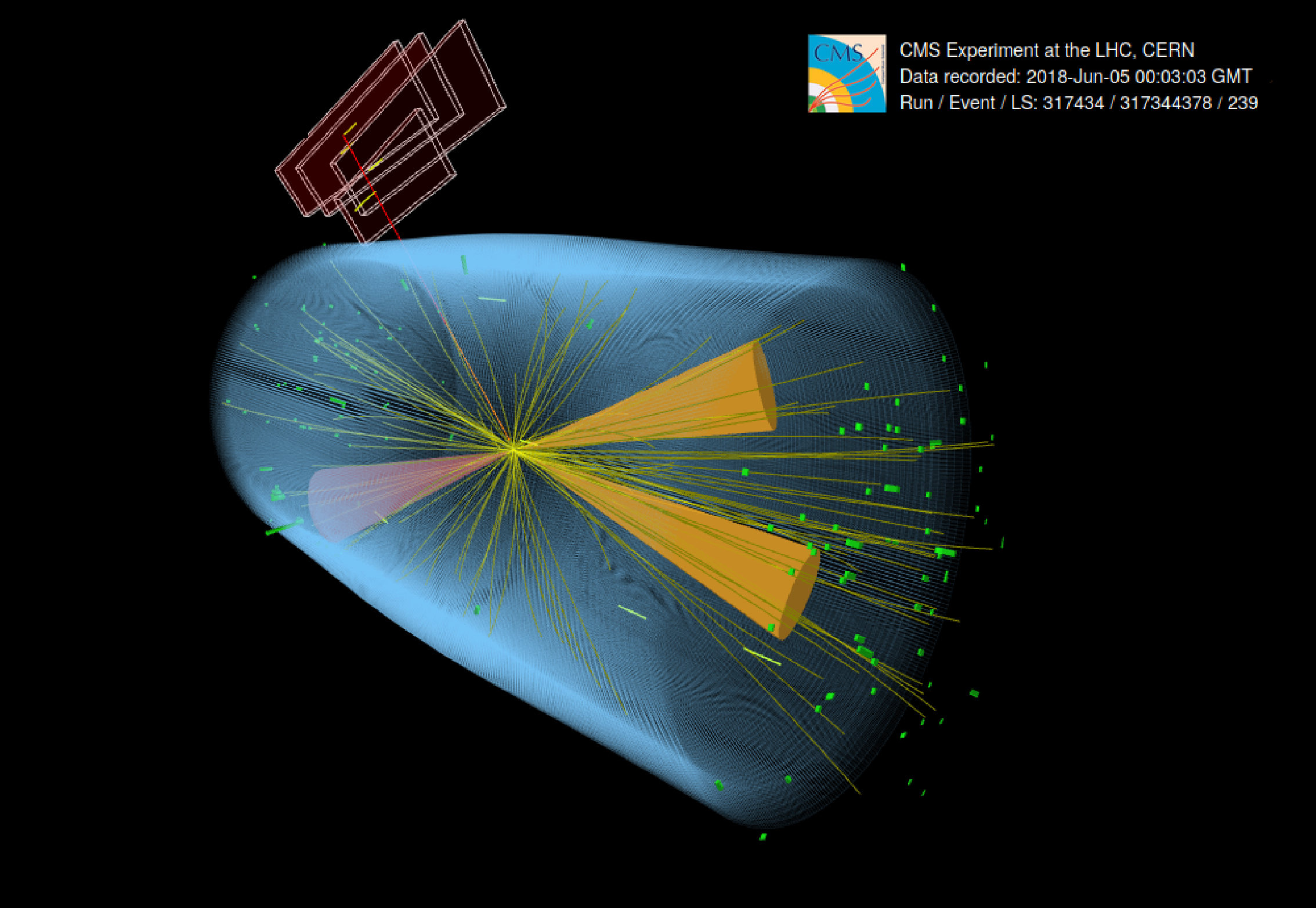
Display of an event with $y_{\text {Signal}}= $ 0.70 in the $ {{\mu}} {\tau}_{\text {h}} $ final state in the 2018 data set. In addition to the b jets, indicated by orange cones, a $ {{\mu}}$ (red line) and a $ {\tau}_{\text {h}} $ decay (red cone) are reconstructed. The same event is shown in different views (rectangular versions of displays). |
png pdf |
Additional Figure 47:
Display of an event with $y_{\text {Signal}}= $ 0.70 in the $ {{\mu}} {\tau}_{\text {h}} $ final state in the 2018 data set. In addition to the b jets, indicated by orange cones, a $ {{\mu}}$ (red line) and a $ {\tau}_{\text {h}} $ decay (red cone) are reconstructed. The same event is shown in different views (rectangular versions of displays). |
png pdf |
Additional Figure 48:
Display of an event with $y_{\text {Signal}}= $ 0.70 in the $ {{\mu}} {\tau}_{\text {h}} $ final state in the 2018 data set. In addition to the b jets, indicated by orange cones, a $ {{\mu}}$ (red line) and a $ {\tau}_{\text {h}} $ decay (red cone) are reconstructed. The same event is shown in different views (rectangular versions of displays). |
png pdf |
Additional Figure 49:
Display of an event with $y_{\text {Signal}}= $ 0.70 in the $ {{\mu}} {\tau}_{\text {h}} $ final state in the 2018 data set. In addition to the b jets, indicated by orange cones, a $ {{\mu}}$ (red line) and a $ {\tau}_{\text {h}} $ decay (red cone) are reconstructed. The same event is shown in different views (rectangular versions of displays). |
png pdf |
Additional Figure 50:
Display of an event with $y_{\text {Signal}}= $ 0.70 in the $ {{\mu}} {\tau}_{\text {h}} $ final state in the 2018 data set. In addition to the b jets, indicated by orange cones, a $ {{\mu}}$ (red line) and a $ {\tau}_{\text {h}} $ decay (red cone) are reconstructed. The same event is shown in different views (rectangular versions of displays). |
png pdf |
Additional Figure 51:
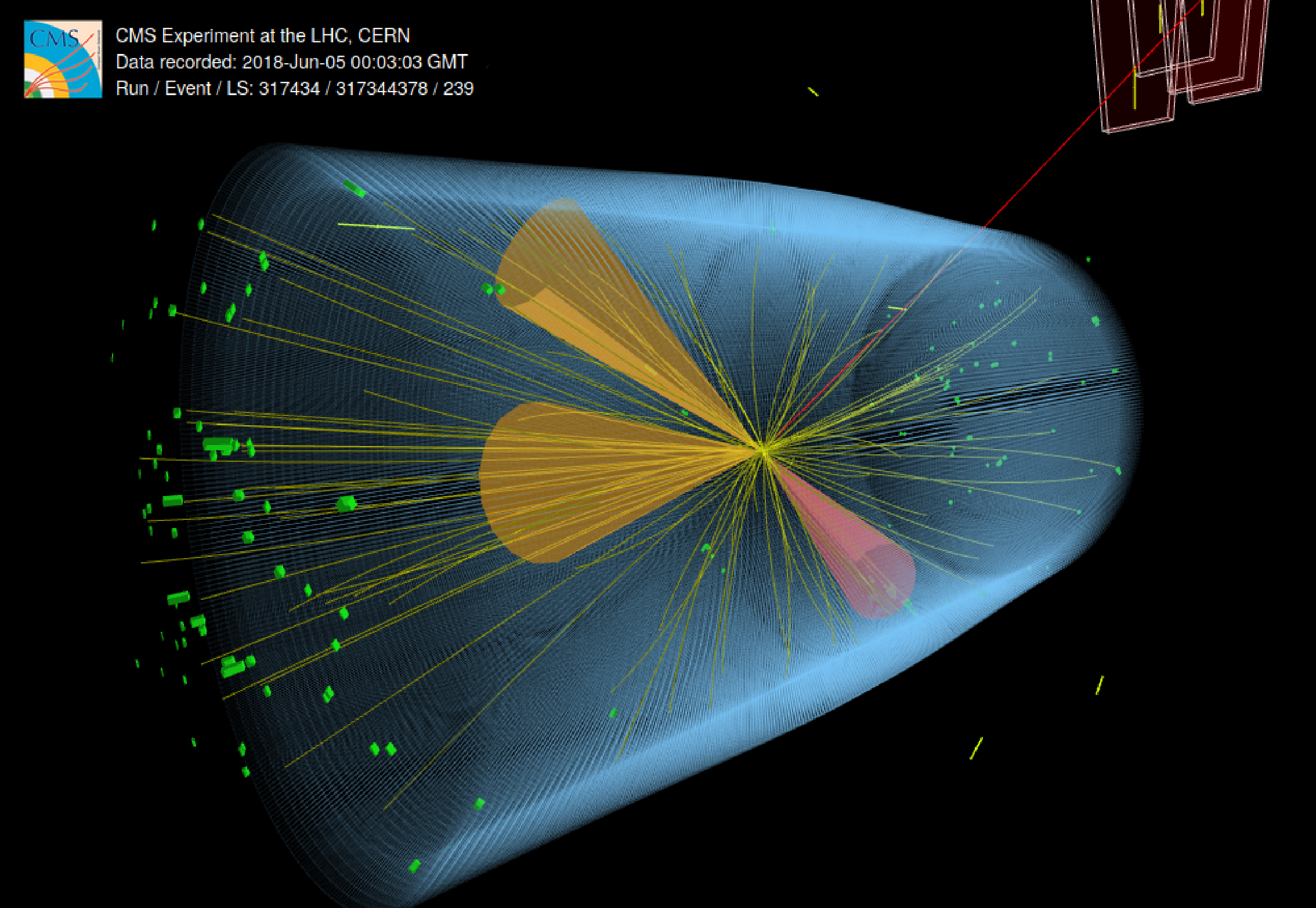
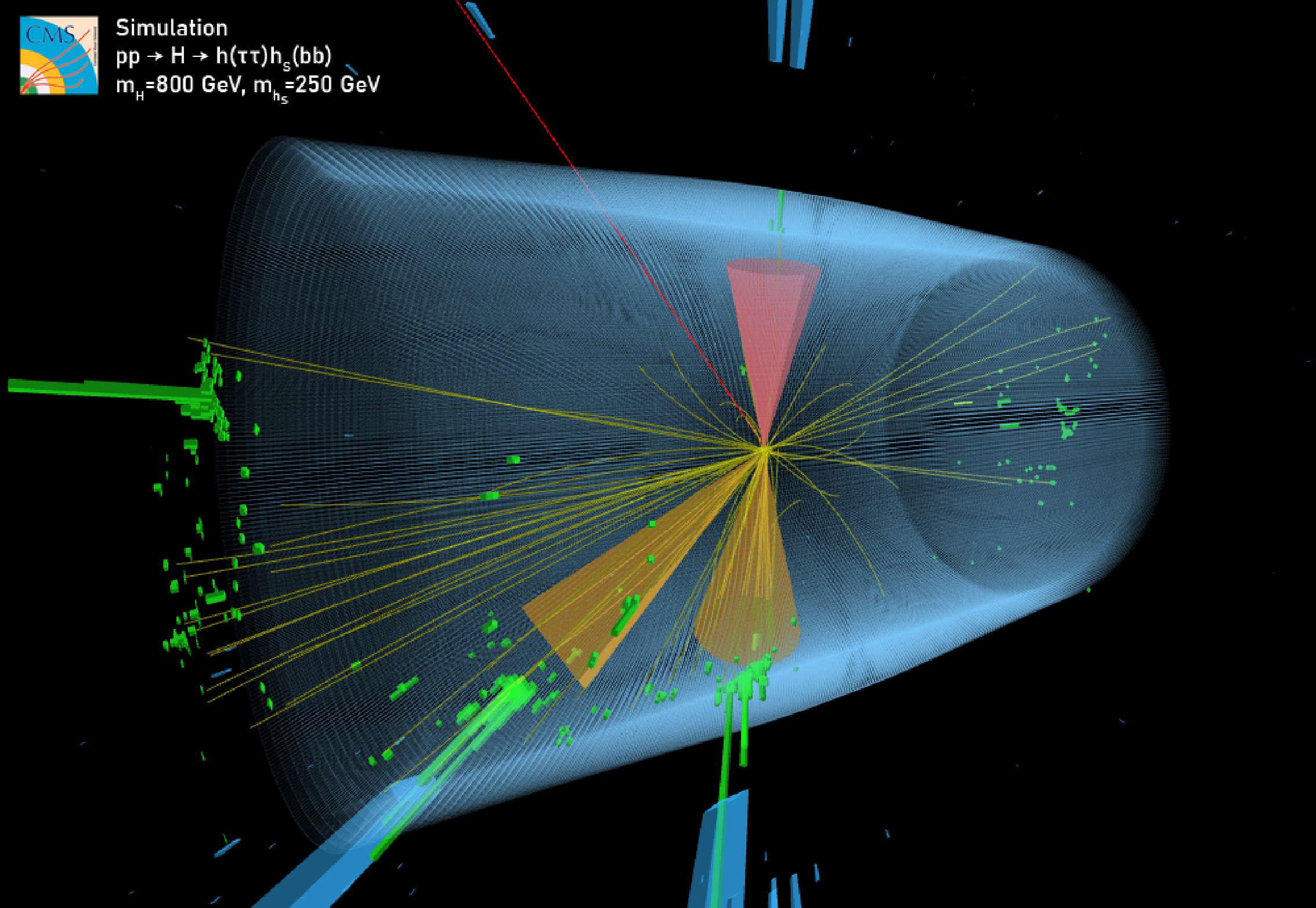
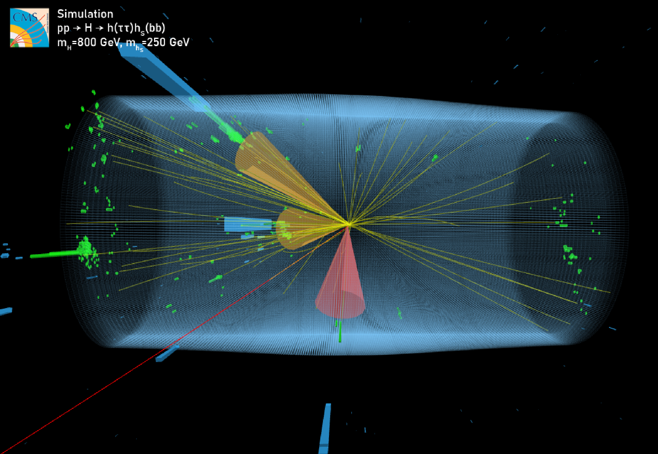
Display of a signal event with $ {m_{{\mathrm {H}}}} = $ 800 GeV and $ {m_{{{\mathrm {h}} _{\text {S}}}}} = $ 250 GeV in the $ {{\mu}} {\tau}_{\text {h}} $ final state from simulation. In addition to the b jets, indicated by orange cones, a $ {{\mu}}$ (red line) and a $ {\tau}_{\text {h}} $ decay (red cone) are reconstructed. The same event is shown in different views (rectangular versions of displays). |
png pdf |
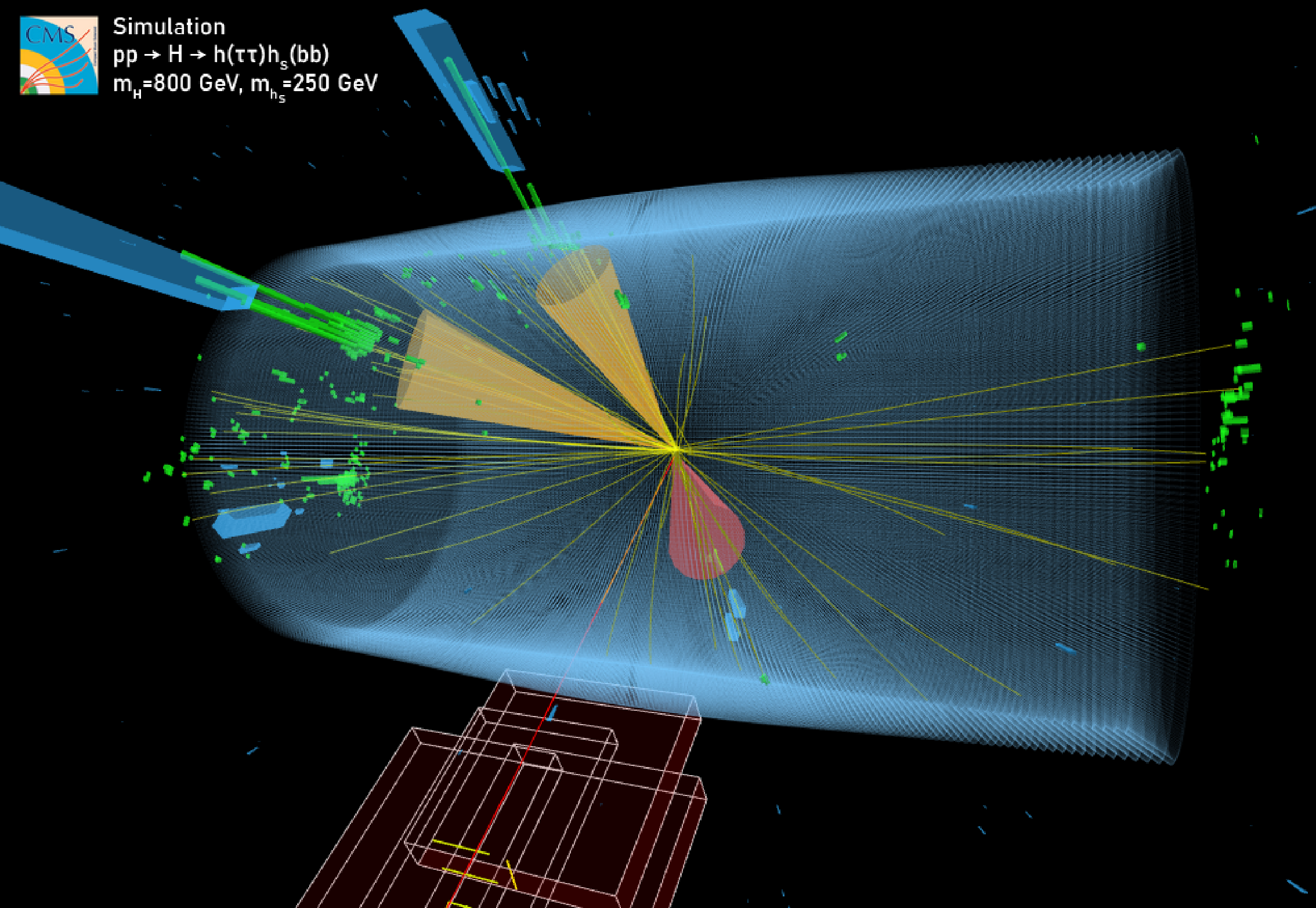
Additional Figure 52:
Display of a signal event with $ {m_{{\mathrm {H}}}} = $ 800 GeV and $ {m_{{{\mathrm {h}} _{\text {S}}}}} = $ 250 GeV in the $ {{\mu}} {\tau}_{\text {h}} $ final state from simulation. In addition to the b jets, indicated by orange cones, a $ {{\mu}}$ (red line) and a $ {\tau}_{\text {h}} $ decay (red cone) are reconstructed. The same event is shown in different views (rectangular versions of displays). |
png pdf |
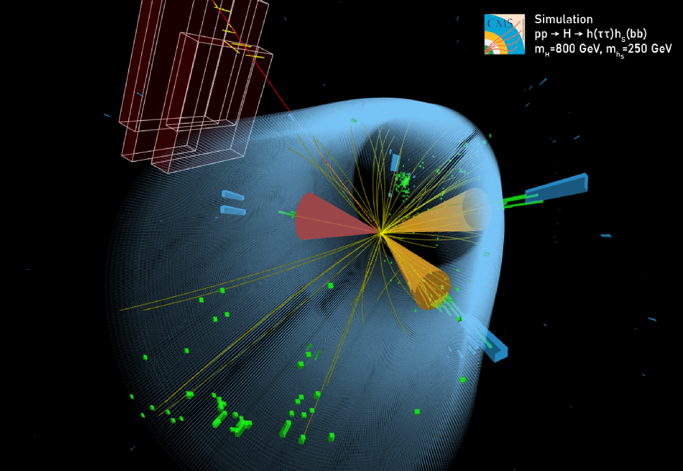
Additional Figure 53:
Display of a signal event with $ {m_{{\mathrm {H}}}} = $ 800 GeV and $ {m_{{{\mathrm {h}} _{\text {S}}}}} = $ 250 GeV in the $ {{\mu}} {\tau}_{\text {h}} $ final state from simulation. In addition to the b jets, indicated by orange cones, a $ {{\mu}}$ (red line) and a $ {\tau}_{\text {h}} $ decay (red cone) are reconstructed. The same event is shown in different views (rectangular versions of displays). |
png pdf |
Additional Figure 54:
Display of a signal event with $ {m_{{\mathrm {H}}}} = $ 800 GeV and $ {m_{{{\mathrm {h}} _{\text {S}}}}} = $ 250 GeV in the $ {{\mu}} {\tau}_{\text {h}} $ final state from simulation. In addition to the b jets, indicated by orange cones, a $ {{\mu}}$ (red line) and a $ {\tau}_{\text {h}} $ decay (red cone) are reconstructed. The same event is shown in different views (rectangular versions of displays). |
png pdf |
Additional Figure 55:
Display of a signal event with $ {m_{{\mathrm {H}}}} = $ 800 GeV and $ {m_{{{\mathrm {h}} _{\text {S}}}}} = $ 250 GeV in the $ {{\mu}} {\tau}_{\text {h}} $ final state from simulation. In addition to the b jets, indicated by orange cones, a $ {{\mu}}$ (red line) and a $ {\tau}_{\text {h}} $ decay (red cone) are reconstructed. The same event is shown in different views (rectangular versions of displays). |
png pdf |
Additional Figure 56:
Display of a signal event with $ {m_{{\mathrm {H}}}} = $ 800 GeV and $ {m_{{{\mathrm {h}} _{\text {S}}}}} = $ 250 GeV in the $ {{\mu}} {\tau}_{\text {h}} $ final state from simulation. In addition to the b jets, indicated by orange cones, a $ {{\mu}}$ (red line) and a $ {\tau}_{\text {h}} $ decay (red cone) are reconstructed. The same event is shown in different views (rectangular versions of displays). |
| Additional Tables | |
png pdf |
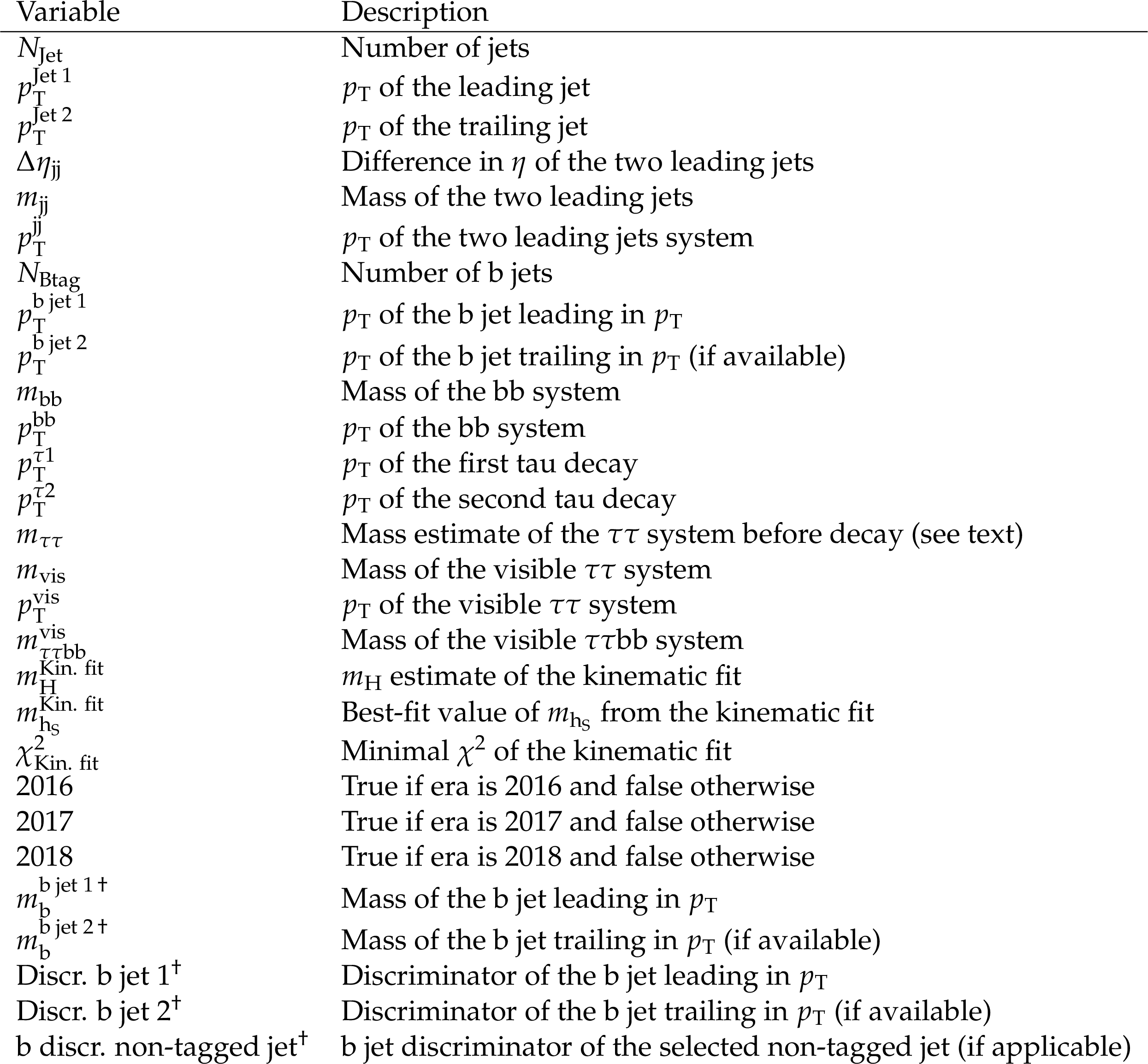
Additional Table 1:
Input variables to the NN training used for event classification. First and second tau decay refer to the position in the final state label. Those entries indicated by $^{\dagger}$ are used in the $ {\tau}_{\text {h}} {\tau}_{\text {h}} $ final state only. Variables that might not be available for a given event are filled with default values. |
| References | ||||
| 1 | ATLAS Collaboration | Observation of a new particle in the search for the standard model Higgs boson with the ATLAS detector at the LHC | PLB 716 (2012) 1 | 1207.7214 |
| 2 | CMS Collaboration | Observation of a new boson at a mass of 125 GeV with the CMS experiment at the LHC | PLB 716 (2012) 30 | CMS-HIG-12-028 1207.7235 |
| 3 | CMS Collaboration | Observation of a new boson with mass near 125 GeV in $ {\mathrm{p}}{\mathrm{p}} $ collisions at $ \sqrt{s} = $ 7 and 8 TeV | JHEP 06 (2013) 081 | CMS-HIG-12-036 1303.4571 |
| 4 | ATLAS and CMS Collaborations | Measurements of the Higgs boson production and decay rates and constraints on its couplings from a combined ATLAS and CMS analysis of the LHC pp collision data at $ \sqrt{s}= $ 7 and 8 TeV | JHEP 08 (2016) 045 | 1606.02266 |
| 5 | CMS Collaboration | Combined measurements of Higgs boson couplings in proton-proton collisions at $ \sqrt{s}= $ 13 TeV | EPJC 79 (2019) 421 | CMS-HIG-17-031 1809.10733 |
| 6 | ATLAS Collaboration | Combined measurements of Higgs boson production and decay using up to 80 fb$ ^{-1} $ of proton-proton collision data at $ \sqrt{s}= $ 13 TeV collected with the ATLAS experiment | PRD 101 (2020) 012002 | 1909.02845 |
| 7 | CMS Collaboration | Measurements of the Higgs boson width and anomalous HVV couplings from on-shell and off-shell production in the four-lepton final state | PRD 99 (2019) 112003 | CMS-HIG-18-002 1901.00174 |
| 8 | Yu. A. Golfand and E. P. Likhtman | Extension of the algebra of Poincaré group generators and violation of p invariance | JEPTL 13 (1971)323 | |
| 9 | J. Wess and B. Zumino | Supergauge transformations in four-dimensions | NPB 70 (1974) 39 | |
| 10 | P. W. Higgs | Broken symmetries, massless particles and gauge fields | PL12 (1964) 132 | |
| 11 | P. W. Higgs | Broken symmetries and the masses of gauge bosons | PRL 13 (1964) 508 | |
| 12 | G. S. Guralnik, C. R. Hagen, and T. W. B. Kibble | Global conservation laws and massless particles | PRL 13 (1964) 585 | |
| 13 | F. Englert and R. Brout | Broken symmetry and the mass of gauge vector mesons | PRL 13 (1964) 321 | |
| 14 | P. W. Higgs | Spontaneous symmetry breakdown without massless bosons | PR145 (1966) 1156 | |
| 15 | T. W. B. Kibble | Symmetry breaking in non-abelian gauge theories | PR155 (1967) 1554 | |
| 16 | P. Fayet | Supergauge invariant extension of the Higgs mechanism and a model for the electron and its neutrino | NPB 90 (1975) 104 | |
| 17 | P. Fayet | Spontaneously broken supersymmetric theories of weak, electromagnetic and strong interactions | PLB 69 (1977) 489 | |
| 18 | J. E. Kim and H. P. Nilles | The $ \mu $-problem and the strong CP problem | PLB 138 (1984) 150 | |
| 19 | U. Ellwanger, C. Hugonie, and A. M. Teixeira | The next-to-minimal supersymmetric standard model | PR 496 (2010) 1 | 0910.1785 |
| 20 | M. Maniatis | The next-to-minimal supersymmetric extension of the standard model reviewed | Int. J. Mod. Phys. A 25 (2010) 3505 | 0906.0777 |
| 21 | ATLAS Collaboration | Search for heavy Higgs bosons decaying into two tau leptons with the ATLAS detector using $ {\mathrm{p}}{\mathrm{p}} $ collisions at $ \sqrt{s}= $ 13 TeV | PRL 125 (2020) 051801 | 2002.12223 |
| 22 | CMS Collaboration | Search for additional neutral MSSM Higgs bosons in the $ \tau\tau $ final state in proton-proton collisions at $ \sqrt{s}= $ 13 TeV | JHEP 09 (2018) 007 | CMS-HIG-17-020 1803.06553 |
| 23 | ATLAS Collaboration | Search for charged Higgs bosons decaying via $ H^{\pm} \to \tau^{\pm}\nu_{\tau} $ in the $ \tau $+jets and $ \tau $+lepton final states with 36 fb$ ^{-1} $ of $ {\mathrm{p}}{\mathrm{p}} $ collision data recorded at $ \sqrt{s} = $ 13 TeV with the ATLAS experiment | JHEP 09 (2018) 139 | 1807.07915 |
| 24 | CMS Collaboration | Search for charged Higgs bosons in the H$ ^{\pm} \to \tau^{\pm}\nu_\tau $ decay channel in proton-proton collisions at $ \sqrt{s} = $ 13 TeV | JHEP 07 (2019) 142 | CMS-HIG-18-014 1903.04560 |
| 25 | S. F. King, M. Muhlleitner, R. Nevzorov, and K. Walz | Discovery prospects for NMSSM Higgs bosons at the high-energy large hadron collider | PRD 90 (2014) 095014 | 1408.1120 |
| 26 | CMS Collaboration | Description and performance of track and primary-vertex reconstruction with the CMS tracker | JINST 9 (2014) P10009 | CMS-TRK-11-001 1405.6569 |
| 27 | CMS Collaboration | Track impact parameter resolution for the full pseudorapidity coverage in the 2017 dataset with the CMS Phase-1 pixel detector | CDS | |
| 28 | CMS Collaboration | Performance of electron reconstruction and selection with the CMS detector in proton-proton collisions at $ \sqrt{s} = $ 8 TeV | JINST 10 (2015) P06005 | CMS-EGM-13-001 1502.02701 |
| 29 | CMS Collaboration | Performance of CMS muon reconstruction in $ {\mathrm{p}}{\mathrm{p}} $ collision events at $ \sqrt{s} = $ 7 TeV | JINST 7 (2012) P10002 | CMS-MUO-10-004 1206.4071 |
| 30 | CMS Collaboration | Performance of photon reconstruction and identification with the CMS detector in proton-proton collisions at $ \sqrt{s}= $ 8 TeV | JINST 10 (2015) P08010 | CMS-EGM-14-001 1502.02702 |
| 31 | CMS Collaboration | Jet energy scale and resolution in the CMS experiment in $ {\mathrm{p}}{\mathrm{p}} $ collisions at 8 TeV | JINST 12 (2017) P02014 | CMS-JME-13-004 1607.03663 |
| 32 | CMS Collaboration | Performance of the CMS Level-1 trigger in proton-proton collisions at $ \sqrt{s} = $ 13 TeV | JINST 15 (2020) P10017 | CMS-TRG-17-001 2006.10165 |
| 33 | CMS Collaboration | The CMS trigger system | JINST 12 (2017) P01020 | CMS-TRG-12-001 1609.02366 |
| 34 | CMS Collaboration | The CMS experiment at the CERN LHC | JINST 3 (2008) S08004 | CMS-00-001 |
| 35 | CMS Collaboration | Particle-flow reconstruction and global event description with the CMS detector | JINST 12 (2017) P10003 | CMS-PRF-14-001 1706.04965 |
| 36 | M. Cacciari, G. P. Salam, and G. Soyez | FastJet user manual | EPJC 72 (2012) 1896 | 1111.6097 |
| 37 | CMS Collaboration | Electron and photon reconstruction and identification with the CMS experiment at the CERN LHC | JINST 16 (2021) P05014 | CMS-EGM-17-001 2012.06888 |
| 38 | CMS Collaboration | Performance of the CMS muon detector and muon reconstruction with proton-proton collisions at $ \sqrt{s}= $ 13 TeV | JINST 13 (2018) P06015 | CMS-MUO-16-001 1804.04528 |
| 39 | CMS Collaboration | Identification of heavy-flavour jets with the CMS detector in pp collisions at 13 TeV | JINST 13 (2018) P05011 | CMS-BTV-16-002 1712.07158 |
| 40 | E. Bols et al. | Jet flavour classification using DeepJet | JINST 15 (2020) P12012 | 2008.10519 |
| 41 | CMS Collaboration | Performance of the DeepJet b tagging algorithm using 41.9/fb of data from proton-proton collisions at 13 TeV with phase-1 CMS detector | CDS | |
| 42 | CMS Collaboration | Performance of reconstruction and identification of $ \tau $ leptons decaying to hadrons and $ \nu_\tau $ in pp collisions at $ \sqrt{s}= $ 13 TeV | JINST 13 (2018) P10005 | CMS-TAU-16-003 1809.02816 |
| 43 | CMS Collaboration | Performance of the DeepTau algorithm for the discrimination of taus against jets, electron, and muons | CDS | |
| 44 | D. Bertolini, P. Harris, M. Low, and N. Tran | Pileup per particle identification | JHEP 10 (2014) 059 | 1407.6013 |
| 45 | CMS Collaboration | Performance of missing transverse momentum reconstruction in proton-proton collisions at $ \sqrt{s} = $ 13 TeV using the CMS detector | JINST 14 (2019) P07004 | CMS-JME-17-001 1903.06078 |
| 46 | CMS Collaboration | An embedding technique to determine $ \tau\tau $ backgrounds in proton-proton collision data | JINST 14 (2019) P06032 | CMS-TAU-18-001 1903.01216 |
| 47 | CMS Collaboration | Measurement of the $ \mathrm{Z}\gamma^{*} \to \tau\tau $ cross section in pp collisions at $ \sqrt{s} = $ 13 TeV and validation of $ \tau $ lepton analysis techniques | EPJC 78 (2018) 708 | CMS-HIG-15-007 1801.03535 |
| 48 | J. Alwall et al. | MadGraph 5: Going beyond | JHEP 06 (2011) 128 | 1106.0522 |
| 49 | J. Alwall et al. | The automated computation of tree-level and next-to-leading order differential cross sections, and their matching to parton shower simulations | JHEP 07 (2014) 079 | 1405.0301 |
| 50 | P. Nason | A new method for combining NLO QCD with shower Monte Carlo algorithms | JHEP 11 (2004) 040 | hep-ph/0409146 |
| 51 | S. Frixione, P. Nason, and C. Oleari | Matching NLO QCD computations with parton shower simulations: the POWHEG method | JHEP 11 (2007) 070 | 0709.2092 |
| 52 | S. Alioli, P. Nason, C. Oleari, and E. Re | NLO Higgs boson production via gluon fusion matched with shower in POWHEG | JHEP 04 (2009) 002 | 0812.0578 |
| 53 | S. Alioli, P. Nason, C. Oleari, and E. Re | A general framework for implementing NLO calculations in shower Monte Carlo programs: the POWHEG BOX | JHEP 06 (2010) 043 | 1002.2581 |
| 54 | S. Alioli et al. | Jet pair production in POWHEG | JHEP 04 (2011) 081 | 1012.3380 |
| 55 | E. Bagnaschi, G. Degrassi, P. Slavich, and A. Vicini | Higgs production via gluon fusion in the POWHEG approach in the SM and in the MSSM | JHEP 02 (2012) 088 | 1111.2854 |
| 56 | K. Melnikov and F. Petriello | Electroweak gauge boson production at hadron colliders through $ \mathcal{O}(\alpha_\text{s}^{2}) $ | PRD 74 (2006) 114017 | hep-ph/0609070 |
| 57 | M. Czakon and A. Mitov | Top++: A program for the calculation of the top-pair cross-section at hadron colliders | CPC 185 (2014) 2930 | 1112.5675 |
| 58 | N. Kidonakis | Top quark production | in Proceedings, Helmholtz International Summer School on Physics of Heavy Quarks and Hadrons (HQ 2013): JINR, Dubna, Russia, 2013 | 1311.0283 |
| 59 | J. M. Campbell, R. K. Ellis, and C. Williams | Vector boson pair production at the LHC | JHEP 07 (2011) 018 | 1105.0020 |
| 60 | T. Gehrmann et al. | $ W^+W^- $ production at hadron colliders in next to next to leading order QCD | PRL 113 (2014) 212001 | 1408.5243 |
| 61 | NNPDF Collaboration | Parton distributions for the LHC run II | JHEP 04 (2015) 040 | 1410.8849 |
| 62 | NNPDF Collaboration | Parton distributions from high-precision collider data | EPJC 77 (2017) 663 | 1706.00428 |
| 63 | CMS Collaboration | Event generator tunes obtained from underlying event and multiparton scattering measurements | EPJC 76 (2016) 155 | CMS-GEN-14-001 1512.00815 |
| 64 | CMS Collaboration | Extraction and validation of a new set of CMS PYTHIA8 tunes from underlying-event measurements | EPJC 80 (2020) 4 | CMS-GEN-17-001 1903.12179 |
| 65 | T. Sjostrand et al. | An introduction to PYTHIA 8.2 | CPC 191 (2015) 159 | 1410.3012 |
| 66 | S. Agostinelli et al. | GEANT4--a simulation toolkit | NIMA 506 (2003) 250 | |
| 67 | CMS Collaboration | Measurements of inclusive $ \mathrm{W} $ and $ \mathrm{Z} $ cross sections in $ {\mathrm{p}}{\mathrm{p}} $ collisions at $ \sqrt{s} = $ 7 TeV | JHEP 01 (2011) 080 | CMS-EWK-10-002 1012.2466 |
| 68 | CMS Collaboration | Measurement of the differential cross section for top quark pair production in pp collisions at $ \sqrt{s} = $ 8 TeV | EPJC 75 (2015) 542 | CMS-TOP-12-028 1505.04480 |
| 69 | S. Baker and R. D. Cousins | Clarification of the use of chi square and likelihood functions in fits to histograms | NIM221 (1984) 437 | |
| 70 | CMS Collaboration | A deep neural network for simultaneous estimation of b jet energy and resolution | Comput. Softw. Big Sci. 4 (2020) 10 | CMS-HIG-18-027 1912.06046 |
| 71 | M. Abadi et al. | TensorFlow: Large-scale machine learning on heterogeneous systems | 2015 Software available from tensorflow.org. \url https://www.tensorflow.org/ | |
| 72 | L. Bianchini, J. Conway, E. K. Friis, and C. Veelken | Reconstruction of the Higgs mass in $ \mathrm{H}\to\tau\tau $ events by dynamical likelihood techniques | J. Phys. Conf. Ser. 513 (2014) 022035 | |
| 73 | CMS Collaboration | Searches for a heavy scalar boson H decaying to a pair of 125 GeV Higgs bosons hh or for a heavy pseudoscalar boson A decaying to Zh, in the final states with $ \text{h}\to\tau\tau $ | PLB 755 (2016) 217 | CMS-HIG-14-034 1510.01181 |
| 74 | S. Wunsch, R. Friese, R. Wolf, and G. Quast | Identifying the relevant dependencies of the neural network response on characteristics of the input space | Comput. Softw. Big Sci. 2 (2018) 5 | 1803.08782 |
| 75 | X. Glorot and Y. Bengio | Understanding the difficulty of training deep feedforward neural networks | in Proceedings of the Thirteenth International Conference on Artificial Intelligence and Statistics, Y. W. Teh and M. Titterington, eds., volume 9 of Proceedings of Machine Learning Research, PMLR, Chia Laguna Resort, Sardinia, Italy | |
| 76 | R. Shimizu et al. | Balanced mini-batch training for imbalanced image data classification with neural network | in 2018 First International Conference on Artificial Intelligence for Industries (AI4I), 2018 | |
| 77 | D. P. Kingma and J. Ba | Adam: A method for stochastic optimization | 1412.6980 | |
| 78 | A. N. Tikhonov | Solution of incorrectly formulated problems and the regularization method | Soviet Math. Dokl. 4 (1963) 1035 | |
| 79 | R. J. Barlow and C. Beeston | Fitting using finite Monte Carlo samples | CPC 77 (1993) 219 | |
| 80 | CMS Collaboration | Precision luminosity measurement in proton-proton collisions at $ \sqrt{s} = $ 13 TeV in 2015 and 2016 at CMS | Submitted to EPJC | CMS-LUM-17-003 2104.01927 |
| 81 | CMS Collaboration | CMS luminosity measurement for the 2017 data taking period at $ \sqrt{s}= $ 13 TeV | CMS-PAS-LUM-17-004 | CMS-PAS-LUM-17-004 |
| 82 | CMS Collaboration | CMS luminosity measurements for the 2016 data taking period | CMS-PAS-LUM-17-001 | CMS-PAS-LUM-17-001 |
| 83 | CMS Collaboration | CMS luminosity measurement for the 2018 data-taking period at $ \sqrt{s}= $ 13 TeV | CMS-PAS-LUM-18-002 | CMS-PAS-LUM-18-002 |
| 84 | P. Nason and C. Oleari | NLO Higgs boson production via vector-boson fusion matched with shower in POWHEG | JHEP 02 (2010) 037 | 0911.5299 |
| 85 | G. Luisoni, P. Nason, C. Oleari, and F. Tramontano | HW$^{\pm} $/HZ+0 and 1 jet at NLO with the POWHEG BOX interfaced to GoSam and their merging within MiNLO | JHEP 10 (2013) 083 | 1306.2542 |
| 86 | H. B. Hartanto, B. Jager, L. Reina, and D. Wackeroth | Higgs boson production in association with top quarks in the POWHEG BOX | PRD 91 (2015) 094003 | 1501.04498 |
| 87 | LHC Higgs Cross Section Working Group | Handbook of LHC Higgs cross sections: 4. deciphering the nature of the Higgs sector | technical report, CERN | 1610.07922 |
| 88 | The ATLAS Collaboration, The CMS Collaboration, The LHC Higgs Combination Group | Procedure for the LHC Higgs boson search combination in Summer 2011 | CMS-NOTE-2011-005 | |
| 89 | T. Junk | Confidence level computation for combining searches with small statistics | NIMA 434 (1999) 435 | hep-ex/9902006 |
| 90 | A. L. Read | Presentation of search results: The CL$ _{\text{s}} $ technique | JPG 28 (2002) 2693 | |
| 91 | CMS Collaboration | Combined results of searches for the standard model Higgs boson in $ {\mathrm{p}}{\mathrm{p}} $ collisions at $ \sqrt{s} = $ 7 TeV | PLB 710 (2012) 26 | CMS-HIG-11-032 1202.1488 |
| 92 | G. Cowan, K. Cranmer, E. Gross, and O. Vitells | Asymptotic formulae for likelihood-based tests of new physics | EPJC 71 (2011) 1554 | 1007.1727 |
| 93 | U. Ellwanger and C. Hugonie | NMHDECAY 2.0: An updated program for sparticle masses, Higgs masses, couplings and decay widths in the NMSSM | CPC 175 (2006) 290 | hep-ph/0508022 |
| 94 | J. Baglio et al. | NMSSMCALC: A program package for the calculation of loop-corrected Higgs boson masses and decay widths in the (complex) NMSSM | CPC 185 (2014) 3372 | 1312.4788 |
|
|
Compact Muon Solenoid LHC, CERN |
|

|

|

|

|

|