

Compact Muon Solenoid
LHC, CERN
| CMS-HIG-22-011 ; CERN-EP-2024-026 | ||
| Search for ZZ and ZH production in the $ \mathrm{b} \bar{\mathrm{b}}\mathrm{b} \bar{\mathrm{b}} $ final state using proton-proton collisions at $ \sqrt{s}= $ 13 TeV | ||
| CMS Collaboration | ||
| 29 March 2024 | ||
| Submitted to Eur. Phys. J. C | ||
| Abstract: A search for ZZ and ZH production in the $ \mathrm{b} \bar{\mathrm{b}}\mathrm{b} \bar{\mathrm{b}} $ final state is presented, where H is the standard model (SM) Higgs boson. The search uses an event sample of proton-proton collisions corresponding to an integrated luminosity of 133 fb$ ^{-1} $ collected at a center-of-mass energy of 13 TeV with the CMS detector at the CERN LHC. The analysis introduces several novel techniques for deriving and validating a multi-dimensional background model based on control samples in data. A multiclass multivariate classifier customized for the $ \mathrm{b} \bar{\mathrm{b}}\mathrm{b} \bar{\mathrm{b}} $ final state is developed to derive the background model and extract the signal. The data are found to be consistent, within uncertainties, with the SM predictions. The observed (expected) upper limits at 95% confidence level are found to be 3.8 (3.8) and 5.0 (2.9) times the SM prediction for the ZZ and ZH production cross sections, respectively. | ||
| Links: e-print arXiv:2403.20241 [hep-ex] (PDF) ; CDS record ; inSPIRE record ; CADI line (restricted) ; | ||
| Figures & Tables | Summary | Additional Figures | References | CMS Publications |
|---|
| Figures | |
png pdf |
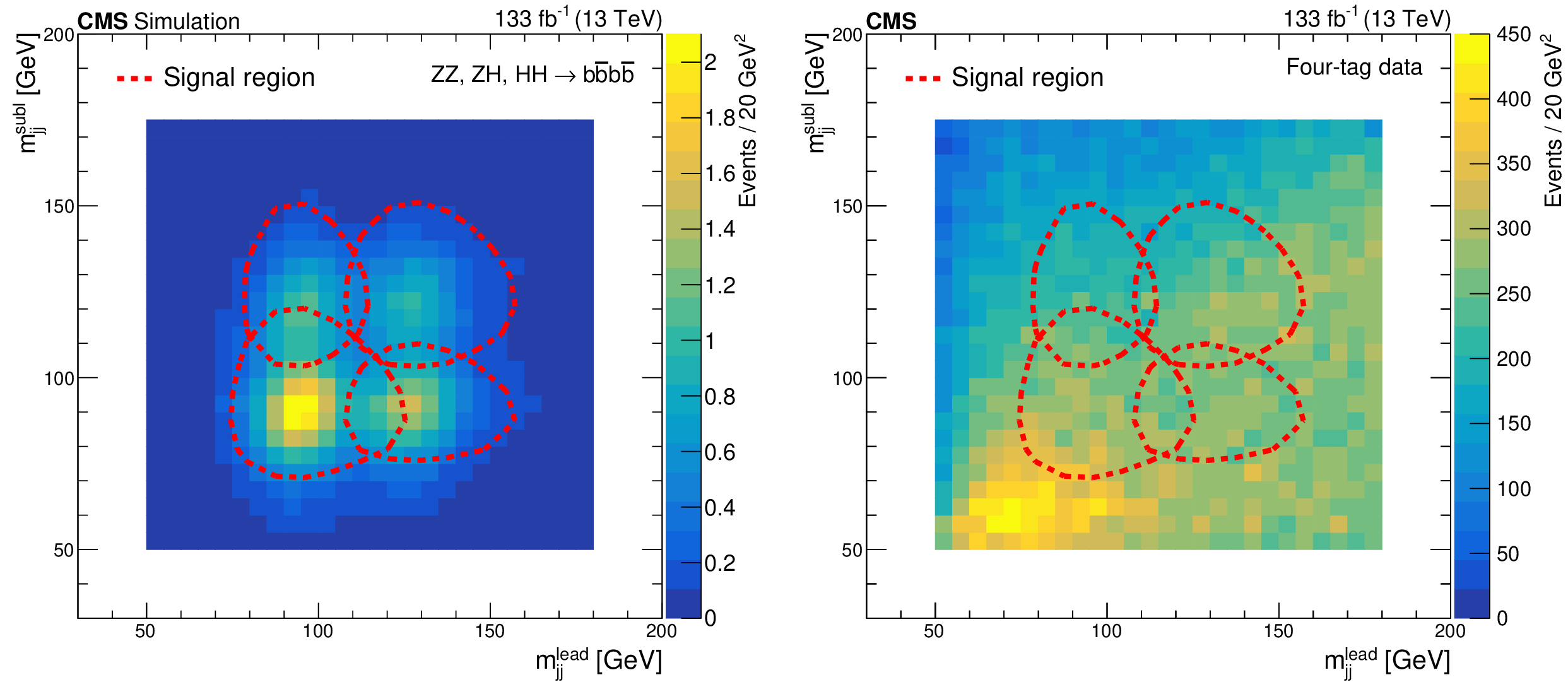
Figure 1:
Signal yield from simulation (left) and from four-tag events in data (right), as a function of $ m_{\mathrm{jj}}^{\text{lead}} $ and $ m_{\mathrm{jj}}^{\text{subl}} $. The color scale to the right of each plot gives the range of values. The signal region is defined by the union of the regions enclosed by the dashed red contours. |
png pdf |
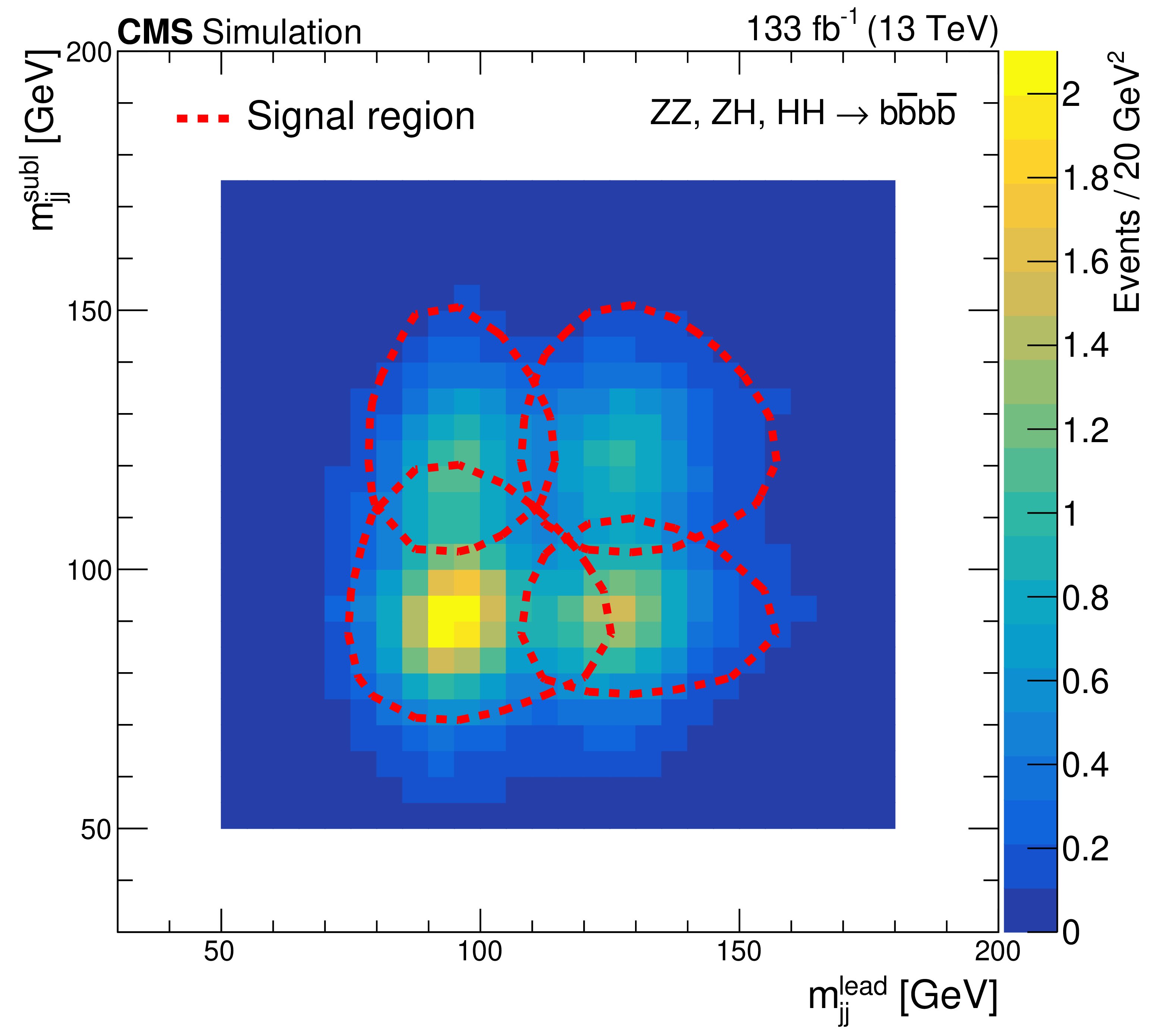
Figure 1-a:
Signal yield from simulation (left) and from four-tag events in data (right), as a function of $ m_{\mathrm{jj}}^{\text{lead}} $ and $ m_{\mathrm{jj}}^{\text{subl}} $. The color scale to the right of each plot gives the range of values. The signal region is defined by the union of the regions enclosed by the dashed red contours. |

png pdf |
Figure 1-b:
Signal yield from simulation (left) and from four-tag events in data (right), as a function of $ m_{\mathrm{jj}}^{\text{lead}} $ and $ m_{\mathrm{jj}}^{\text{subl}} $. The color scale to the right of each plot gives the range of values. The signal region is defined by the union of the regions enclosed by the dashed red contours. |

png pdf |
Figure 2:
Event selection acceptance times efficiency as a function of the generated four-body mass $ m_{4\mathrm{b}}^{\text{gen}} $ for the ZZ (left) and ZH (right) signals. The plots show the cumulative efficiency with respect to the inclusive sample. The expected $ m_{4\mathrm{b}}^{\text{gen}} $ distributions of the inclusive ZZ and ZH events are shown by the gray-shaded areas with arbitrary normalization. |
png pdf |
Figure 2-a:
Event selection acceptance times efficiency as a function of the generated four-body mass $ m_{4\mathrm{b}}^{\text{gen}} $ for the ZZ (left) and ZH (right) signals. The plots show the cumulative efficiency with respect to the inclusive sample. The expected $ m_{4\mathrm{b}}^{\text{gen}} $ distributions of the inclusive ZZ and ZH events are shown by the gray-shaded areas with arbitrary normalization. |

png pdf |
Figure 2-b:
Event selection acceptance times efficiency as a function of the generated four-body mass $ m_{4\mathrm{b}}^{\text{gen}} $ for the ZZ (left) and ZH (right) signals. The plots show the cumulative efficiency with respect to the inclusive sample. The expected $ m_{4\mathrm{b}}^{\text{gen}} $ distributions of the inclusive ZZ and ZH events are shown by the gray-shaded areas with arbitrary normalization. |
png pdf |
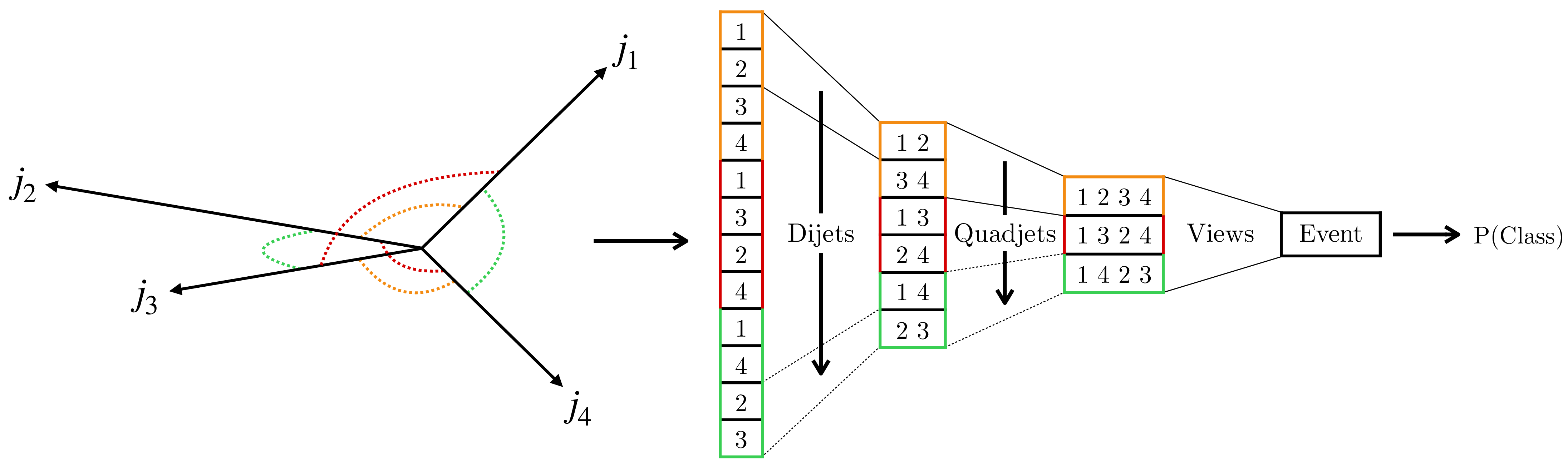
Figure 3:
A high-level sketch of the HCR classifier architecture. Boson-candidate jets are shown on the left with the three possible jet pairings. The HCR architecture is shown on the right. The boxes represent pixels, with the labels indicating which jet, dijet, or quadjet the pixel refers to. The different jet pairings on the left are each represented within the network, as indicated by the color coding. The output P(class) corresponds to the the probability that an event belongs to the corresponding class used in training. |
png pdf |
Figure 4:
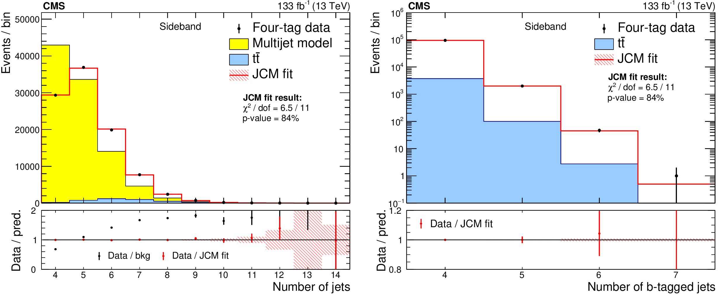
Jet (left) and b-tagged jet (right) multiplicity distributions in the SB region. The black data points show the observed four-tag data, the blue distribution the $ \mathrm{t} \bar{\mathrm{t}} $ simulation, and the yellow histogram the three-tag multijet prior to the JCM corrections. The red histogram shows the result of the fit to the JCM model. The quality of the fit is given by the $ \chi^2 $ per degrees of freedom (dof) and corresponding $ p $-value in the legend. The lower panels display the ratio of the data to the fit prediction. |

png pdf |
Figure 4-a:
Jet (left) and b-tagged jet (right) multiplicity distributions in the SB region. The black data points show the observed four-tag data, the blue distribution the $ \mathrm{t} \bar{\mathrm{t}} $ simulation, and the yellow histogram the three-tag multijet prior to the JCM corrections. The red histogram shows the result of the fit to the JCM model. The quality of the fit is given by the $ \chi^2 $ per degrees of freedom (dof) and corresponding $ p $-value in the legend. The lower panels display the ratio of the data to the fit prediction. |

png pdf |
Figure 4-b:
Jet (left) and b-tagged jet (right) multiplicity distributions in the SB region. The black data points show the observed four-tag data, the blue distribution the $ \mathrm{t} \bar{\mathrm{t}} $ simulation, and the yellow histogram the three-tag multijet prior to the JCM corrections. The red histogram shows the result of the fit to the JCM model. The quality of the fit is given by the $ \chi^2 $ per degrees of freedom (dof) and corresponding $ p $-value in the legend. The lower panels display the ratio of the data to the fit prediction. |
png pdf |
Figure 5:
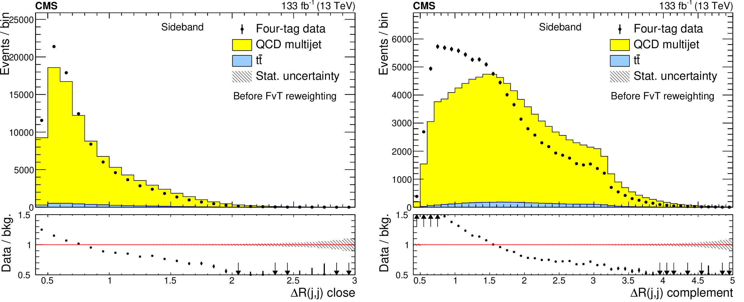
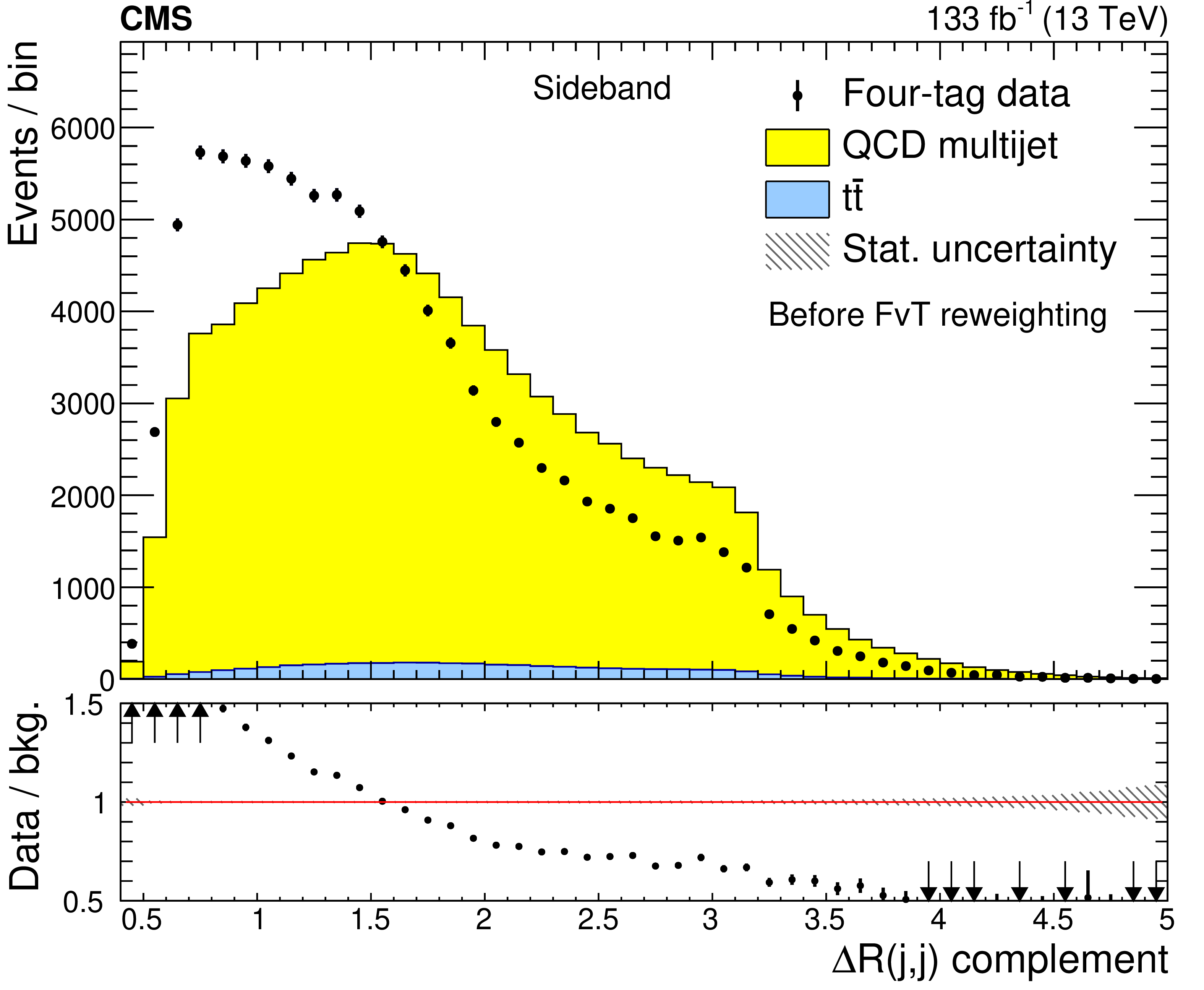
Distributions of $ \Delta \text{R}(j, j)_{\text{close}} $ (left) and $ \Delta \text{R}(j, j)_{\text{complement}} $ (right). The four-tag SB events are shown by the points. The QCD multijet distribution (yellow region) is from the three-tag SB sample after the JCM correction but before the FvT kinematic reweighting, and the $ \mathrm{t} \bar{\mathrm{t}} $ distribution (blue region) is from simulation. The lower panels display the ratio of the four-tag data to the total background, which is the sum of the QCD multijet and $ \mathrm{t} \bar{\mathrm{t}} $ distributions. The hatched area gives the statistical uncertainty in the background. |

png pdf |
Figure 5-a:
Distributions of $ \Delta \text{R}(j, j)_{\text{close}} $ (left) and $ \Delta \text{R}(j, j)_{\text{complement}} $ (right). The four-tag SB events are shown by the points. The QCD multijet distribution (yellow region) is from the three-tag SB sample after the JCM correction but before the FvT kinematic reweighting, and the $ \mathrm{t} \bar{\mathrm{t}} $ distribution (blue region) is from simulation. The lower panels display the ratio of the four-tag data to the total background, which is the sum of the QCD multijet and $ \mathrm{t} \bar{\mathrm{t}} $ distributions. The hatched area gives the statistical uncertainty in the background. |
png pdf |
Figure 5-b:
Distributions of $ \Delta \text{R}(j, j)_{\text{close}} $ (left) and $ \Delta \text{R}(j, j)_{\text{complement}} $ (right). The four-tag SB events are shown by the points. The QCD multijet distribution (yellow region) is from the three-tag SB sample after the JCM correction but before the FvT kinematic reweighting, and the $ \mathrm{t} \bar{\mathrm{t}} $ distribution (blue region) is from simulation. The lower panels display the ratio of the four-tag data to the total background, which is the sum of the QCD multijet and $ \mathrm{t} \bar{\mathrm{t}} $ distributions. The hatched area gives the statistical uncertainty in the background. |
png pdf |
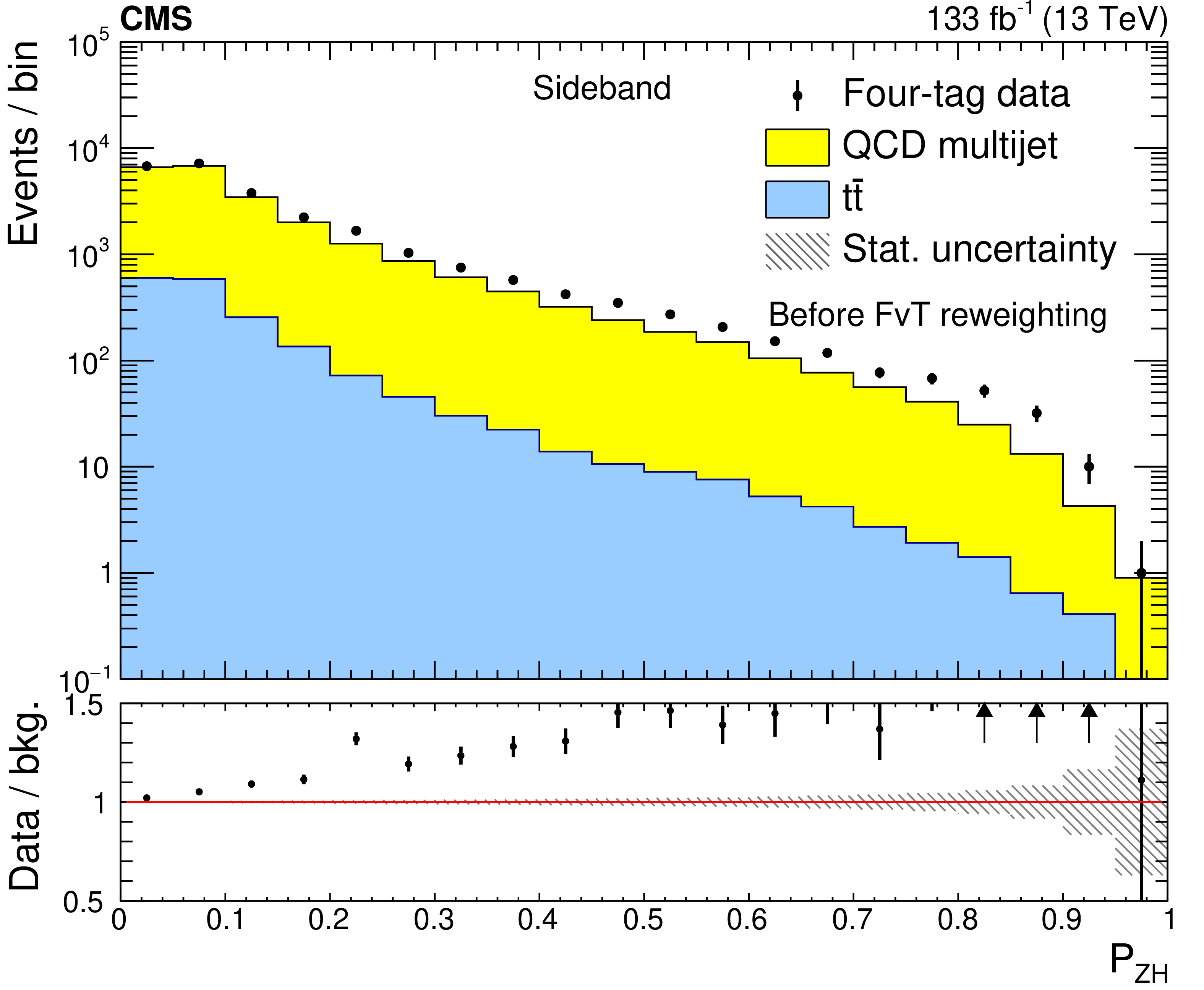
Figure 6:
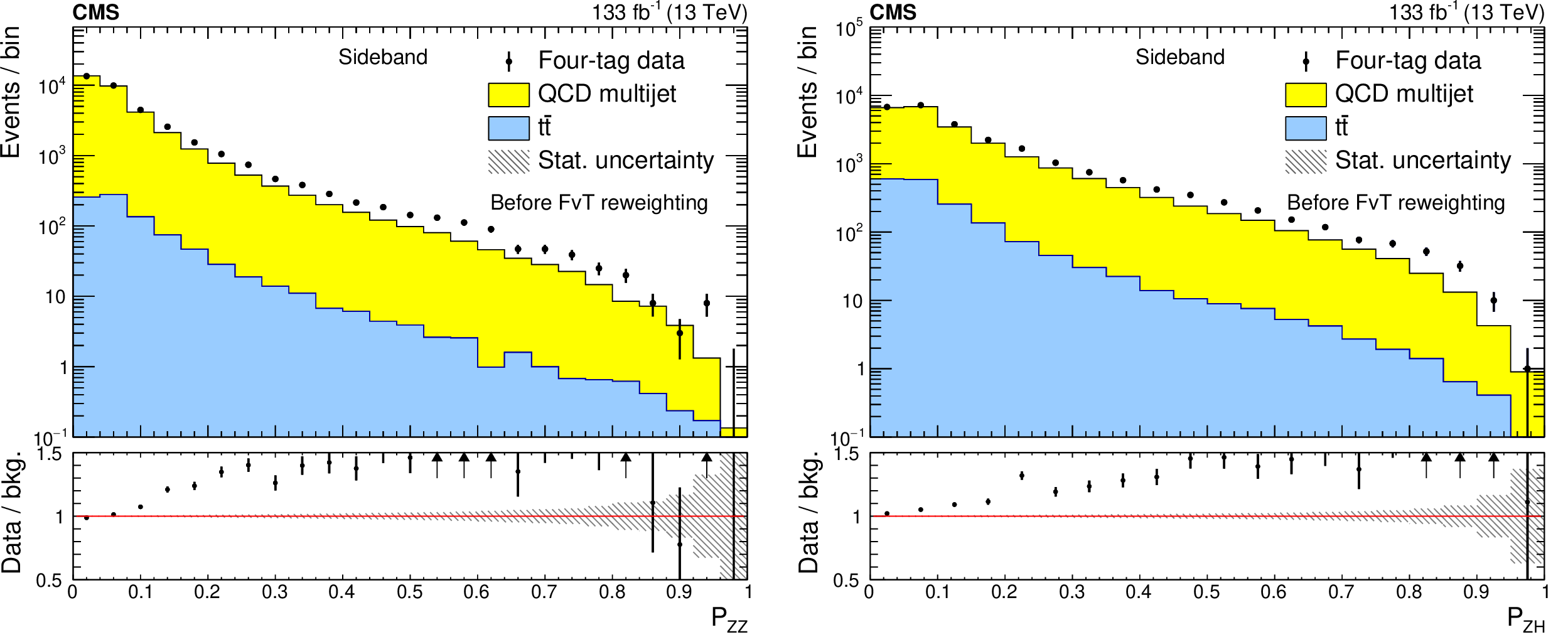
Distributions of the signal probabilities for ZZ (left) and ZH (right) in the SB region, respectively. The four-tag SB events are shown by the points. The QCD multijet distribution (yellow region) is from the three-tag SB sample after the JCM correction but before the FvT kinematic reweighting, and the $ \mathrm{t} \bar{\mathrm{t}} $ distribution (blue region) is from simulation. The lower panels display the ratio of the four-tag data to the total background, which is the sum of the QCD multijet and $ \mathrm{t} \bar{\mathrm{t}} $ distributions. The hatched area gives the statistical uncertainty in the background. |

png pdf |
Figure 6-a:
Distributions of the signal probabilities for ZZ (left) and ZH (right) in the SB region, respectively. The four-tag SB events are shown by the points. The QCD multijet distribution (yellow region) is from the three-tag SB sample after the JCM correction but before the FvT kinematic reweighting, and the $ \mathrm{t} \bar{\mathrm{t}} $ distribution (blue region) is from simulation. The lower panels display the ratio of the four-tag data to the total background, which is the sum of the QCD multijet and $ \mathrm{t} \bar{\mathrm{t}} $ distributions. The hatched area gives the statistical uncertainty in the background. |
png pdf |
Figure 6-b:
Distributions of the signal probabilities for ZZ (left) and ZH (right) in the SB region, respectively. The four-tag SB events are shown by the points. The QCD multijet distribution (yellow region) is from the three-tag SB sample after the JCM correction but before the FvT kinematic reweighting, and the $ \mathrm{t} \bar{\mathrm{t}} $ distribution (blue region) is from simulation. The lower panels display the ratio of the four-tag data to the total background, which is the sum of the QCD multijet and $ \mathrm{t} \bar{\mathrm{t}} $ distributions. The hatched area gives the statistical uncertainty in the background. |
png pdf |
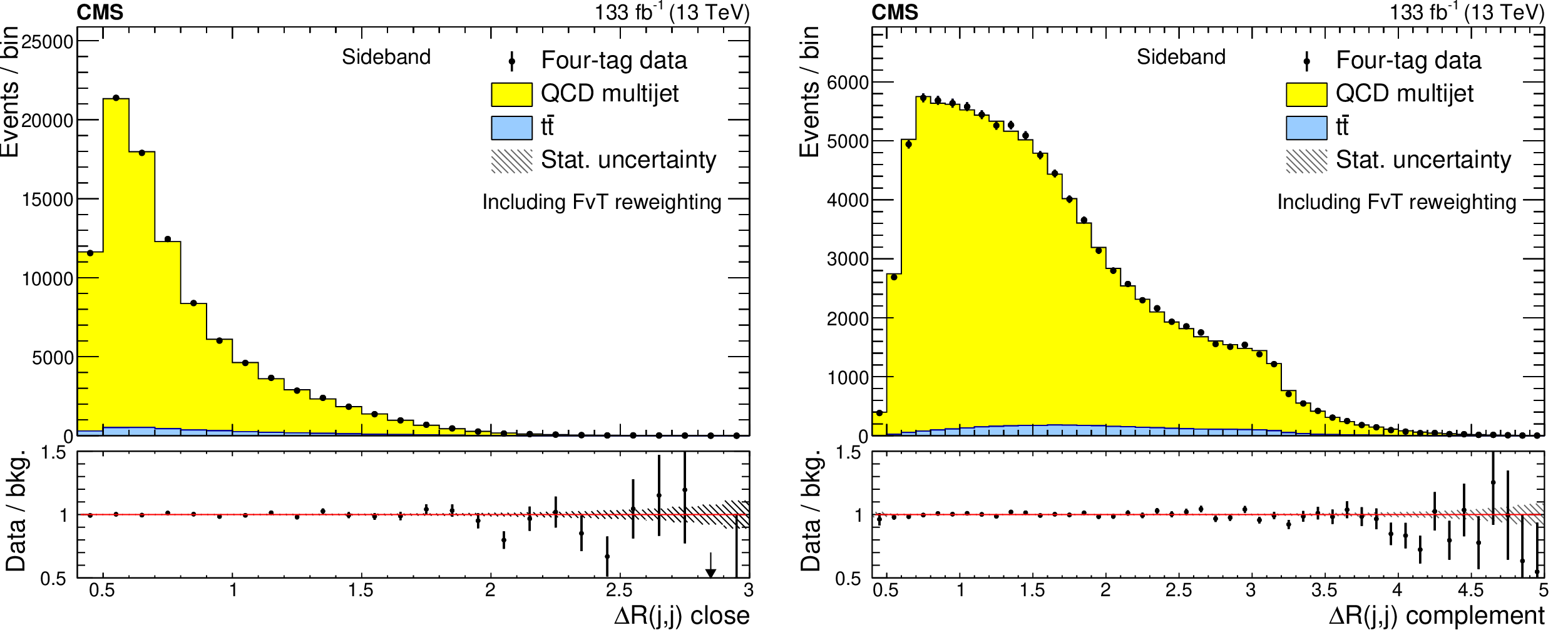
Figure 7:
The $ \Delta\text{R}(j,j) $ distributions shown in Figure 5 after including the FvT corrections to the QCD multijet prediction. |

png pdf |
Figure 7-a:
The $ \Delta\text{R}(j,j) $ distributions shown in Figure 5 after including the FvT corrections to the QCD multijet prediction. |

png pdf |
Figure 7-b:
The $ \Delta\text{R}(j,j) $ distributions shown in Figure 5 after including the FvT corrections to the QCD multijet prediction. |

png pdf |
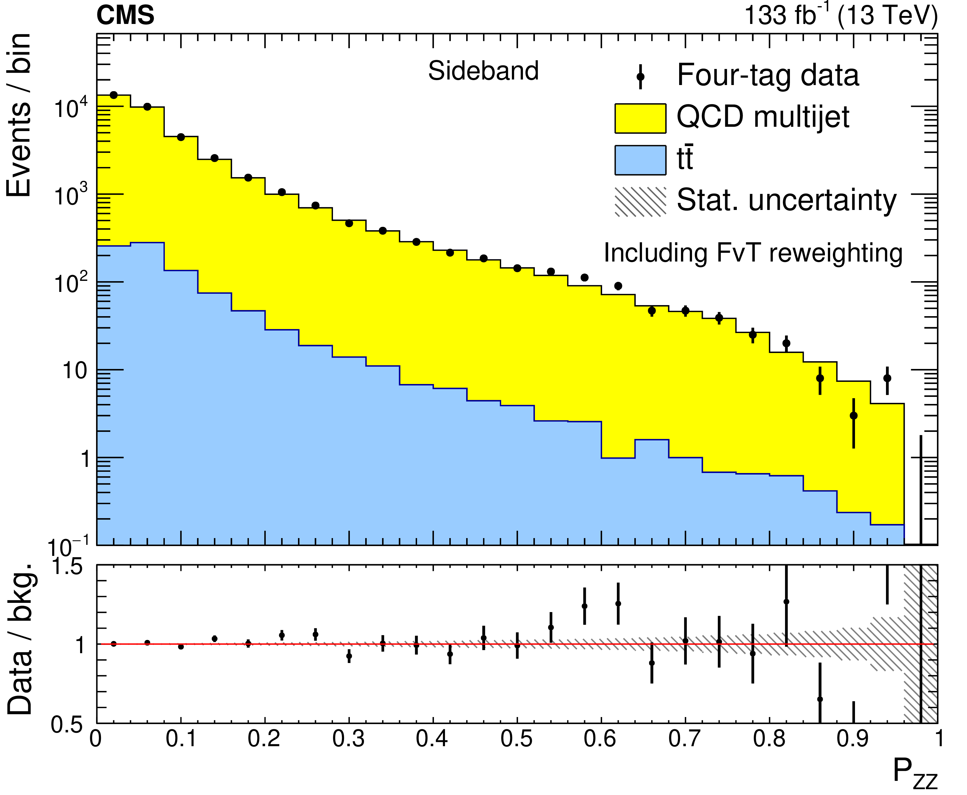
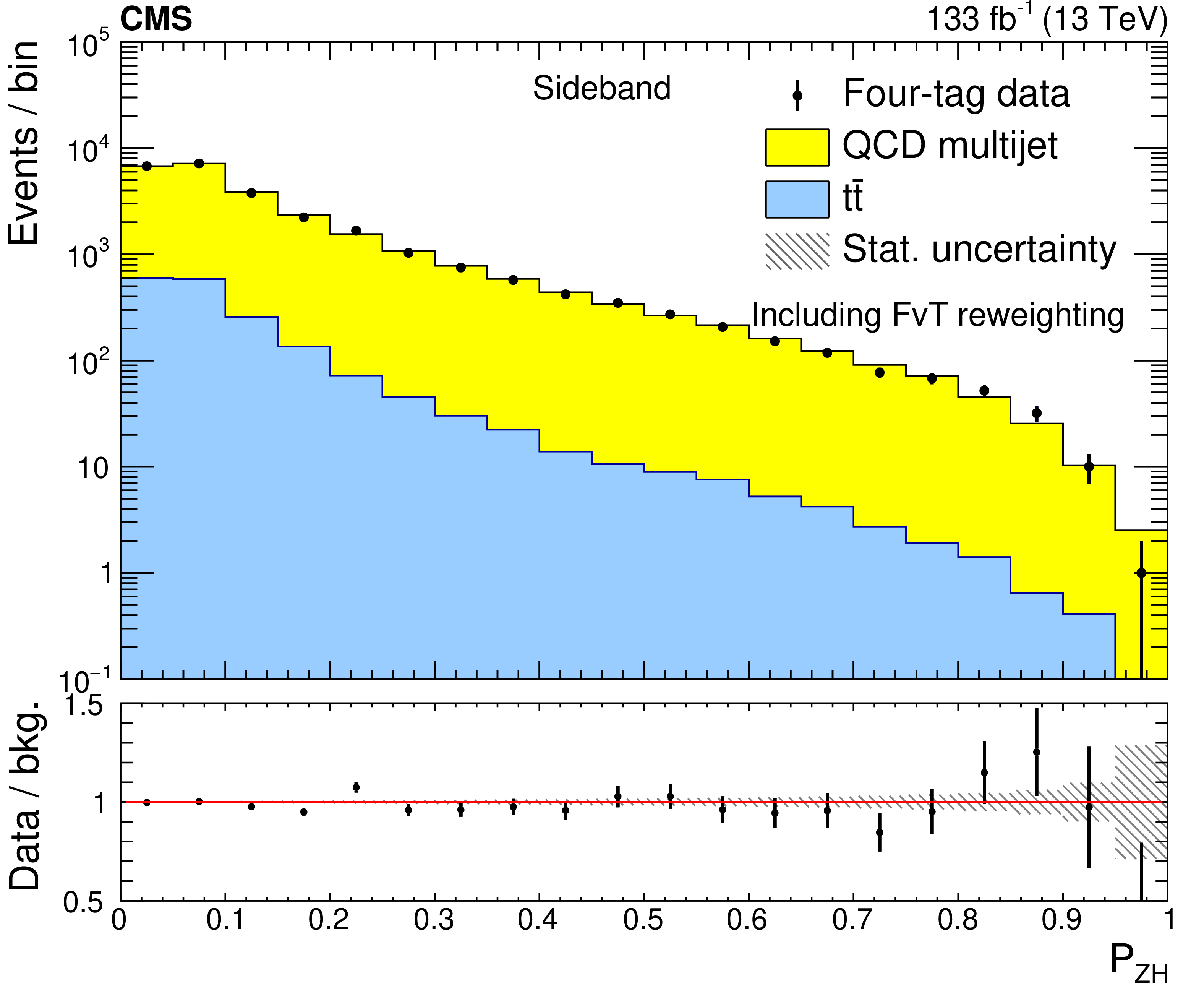
Figure 8:
Distribution of signal probabilities for ZZ (left) and ZH (right) events in the SB region after including the FvT corrections to the QCD multijet prediction. |
png pdf |
Figure 8-a:
Distribution of signal probabilities for ZZ (left) and ZH (right) events in the SB region after including the FvT corrections to the QCD multijet prediction. |
png pdf |
Figure 8-b:
Distribution of signal probabilities for ZZ (left) and ZH (right) events in the SB region after including the FvT corrections to the QCD multijet prediction. |

png pdf |
Figure 9:
An illustration of the hemisphere mixing procedure, adapted from Ref. [20]. Three-tag events are divided into two halves by cutting along the axis perpendicular to the transverse thrust axis. In a preliminary step, each event in the four-tag data set is split into two hemispheres that are collected in a library of hemispheres. Once the library is created, each three-tag event is used as a basis for creating a synthetic event. These are constructed by picking the two hemispheres from the library that are most similar to the hemispheres making up the original event. |
png pdf |
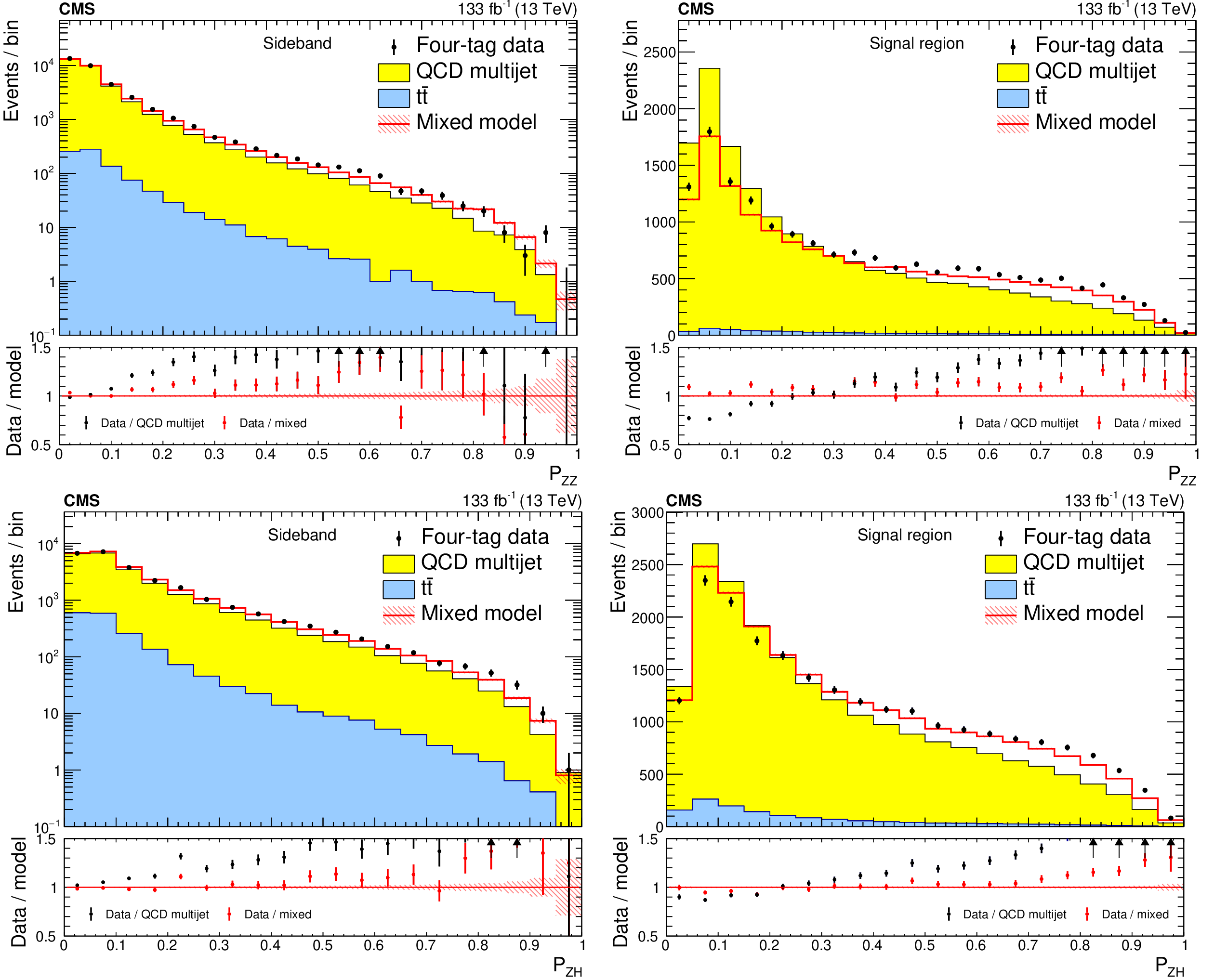
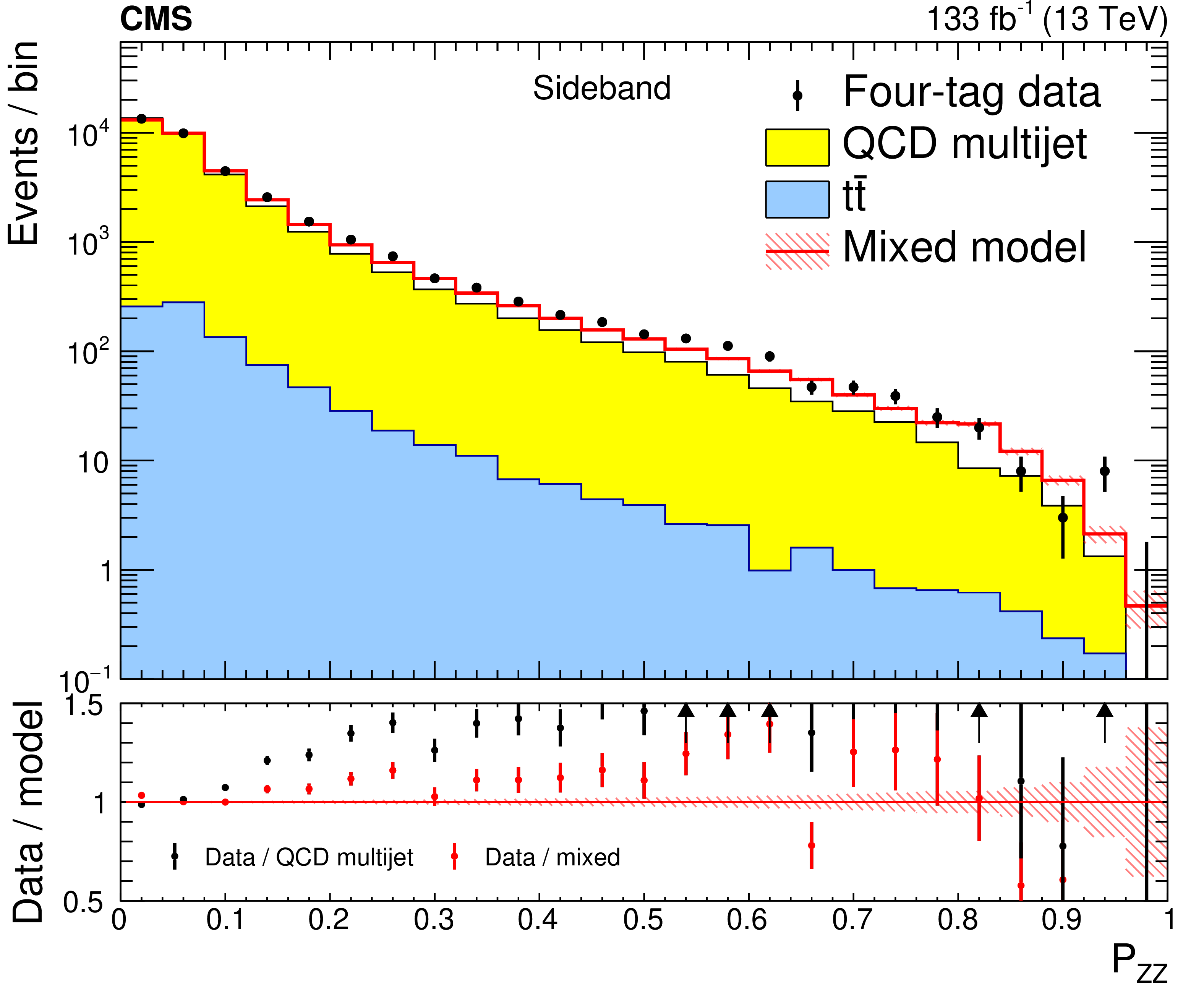
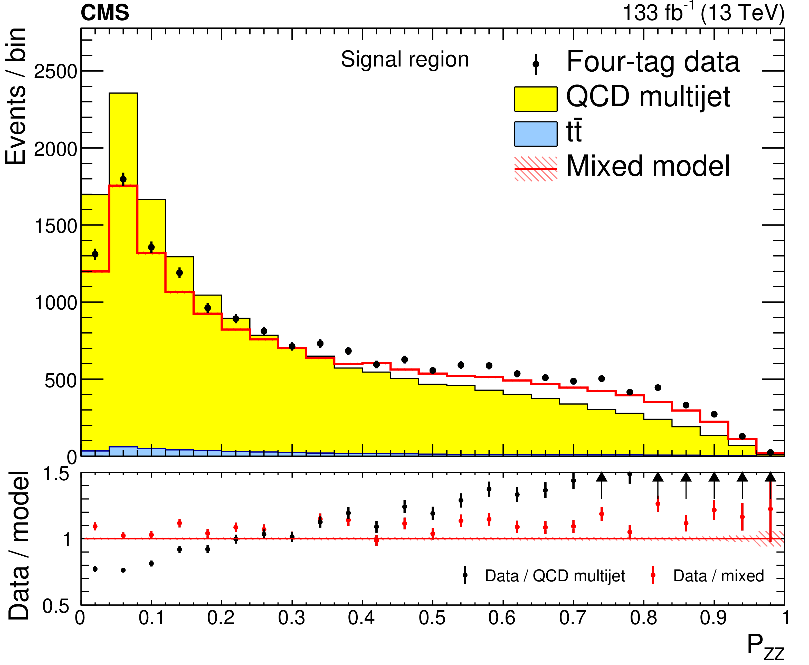
Figure 10:
Distribution of signal probabilities for ZZ (upper row) and ZH (lower row) events in the sideband (left) and signal regions (right). The four-tag events are shown by the points. The QCD multijet distribution before the FvT corrections is given by the yellow region, and the simulated $ \mathrm{t} \bar{\mathrm{t}} $ distribution by the blue area. The average of the mixed models (red) provides a high-event-count proxy of the 4b background (black) that allows the extrapolation of the background model to be tested precisely. The lower panels display the ratio of the four-tag data to the average of the mixed models (red) and to the QCD multijet distribution (black). |
png pdf |
Figure 10-a:
Distribution of signal probabilities for ZZ (upper row) and ZH (lower row) events in the sideband (left) and signal regions (right). The four-tag events are shown by the points. The QCD multijet distribution before the FvT corrections is given by the yellow region, and the simulated $ \mathrm{t} \bar{\mathrm{t}} $ distribution by the blue area. The average of the mixed models (red) provides a high-event-count proxy of the 4b background (black) that allows the extrapolation of the background model to be tested precisely. The lower panels display the ratio of the four-tag data to the average of the mixed models (red) and to the QCD multijet distribution (black). |
png pdf |
Figure 10-b:
Distribution of signal probabilities for ZZ (upper row) and ZH (lower row) events in the sideband (left) and signal regions (right). The four-tag events are shown by the points. The QCD multijet distribution before the FvT corrections is given by the yellow region, and the simulated $ \mathrm{t} \bar{\mathrm{t}} $ distribution by the blue area. The average of the mixed models (red) provides a high-event-count proxy of the 4b background (black) that allows the extrapolation of the background model to be tested precisely. The lower panels display the ratio of the four-tag data to the average of the mixed models (red) and to the QCD multijet distribution (black). |

png pdf |
Figure 10-c:
Distribution of signal probabilities for ZZ (upper row) and ZH (lower row) events in the sideband (left) and signal regions (right). The four-tag events are shown by the points. The QCD multijet distribution before the FvT corrections is given by the yellow region, and the simulated $ \mathrm{t} \bar{\mathrm{t}} $ distribution by the blue area. The average of the mixed models (red) provides a high-event-count proxy of the 4b background (black) that allows the extrapolation of the background model to be tested precisely. The lower panels display the ratio of the four-tag data to the average of the mixed models (red) and to the QCD multijet distribution (black). |

png pdf |
Figure 10-d:
Distribution of signal probabilities for ZZ (upper row) and ZH (lower row) events in the sideband (left) and signal regions (right). The four-tag events are shown by the points. The QCD multijet distribution before the FvT corrections is given by the yellow region, and the simulated $ \mathrm{t} \bar{\mathrm{t}} $ distribution by the blue area. The average of the mixed models (red) provides a high-event-count proxy of the 4b background (black) that allows the extrapolation of the background model to be tested precisely. The lower panels display the ratio of the four-tag data to the average of the mixed models (red) and to the QCD multijet distribution (black). |

png pdf |
Figure 11:
The distributions of the ZZ (left) and ZH (right) signal probabilities. The black data points show the average of the mixed models. The yellow and blue distributions show the average of the QCD multijet models and the $ \mathrm{t} \bar{\mathrm{t}} $ simulation, respectively. The red histogram displays the post-fit results of the data fit to the background model. The ZZ channel data distribution is fit with all five basic coefficients constrained, while the ZH channel distribution has two of the four coefficients unconstrained. The lower panels give the pre- (blue) and post-fit (red) pulls. |

png pdf |
Figure 11-a:
The distributions of the ZZ (left) and ZH (right) signal probabilities. The black data points show the average of the mixed models. The yellow and blue distributions show the average of the QCD multijet models and the $ \mathrm{t} \bar{\mathrm{t}} $ simulation, respectively. The red histogram displays the post-fit results of the data fit to the background model. The ZZ channel data distribution is fit with all five basic coefficients constrained, while the ZH channel distribution has two of the four coefficients unconstrained. The lower panels give the pre- (blue) and post-fit (red) pulls. |

png pdf |
Figure 11-b:
The distributions of the ZZ (left) and ZH (right) signal probabilities. The black data points show the average of the mixed models. The yellow and blue distributions show the average of the QCD multijet models and the $ \mathrm{t} \bar{\mathrm{t}} $ simulation, respectively. The red histogram displays the post-fit results of the data fit to the background model. The ZZ channel data distribution is fit with all five basic coefficients constrained, while the ZH channel distribution has two of the four coefficients unconstrained. The lower panels give the pre- (blue) and post-fit (red) pulls. |

png pdf |
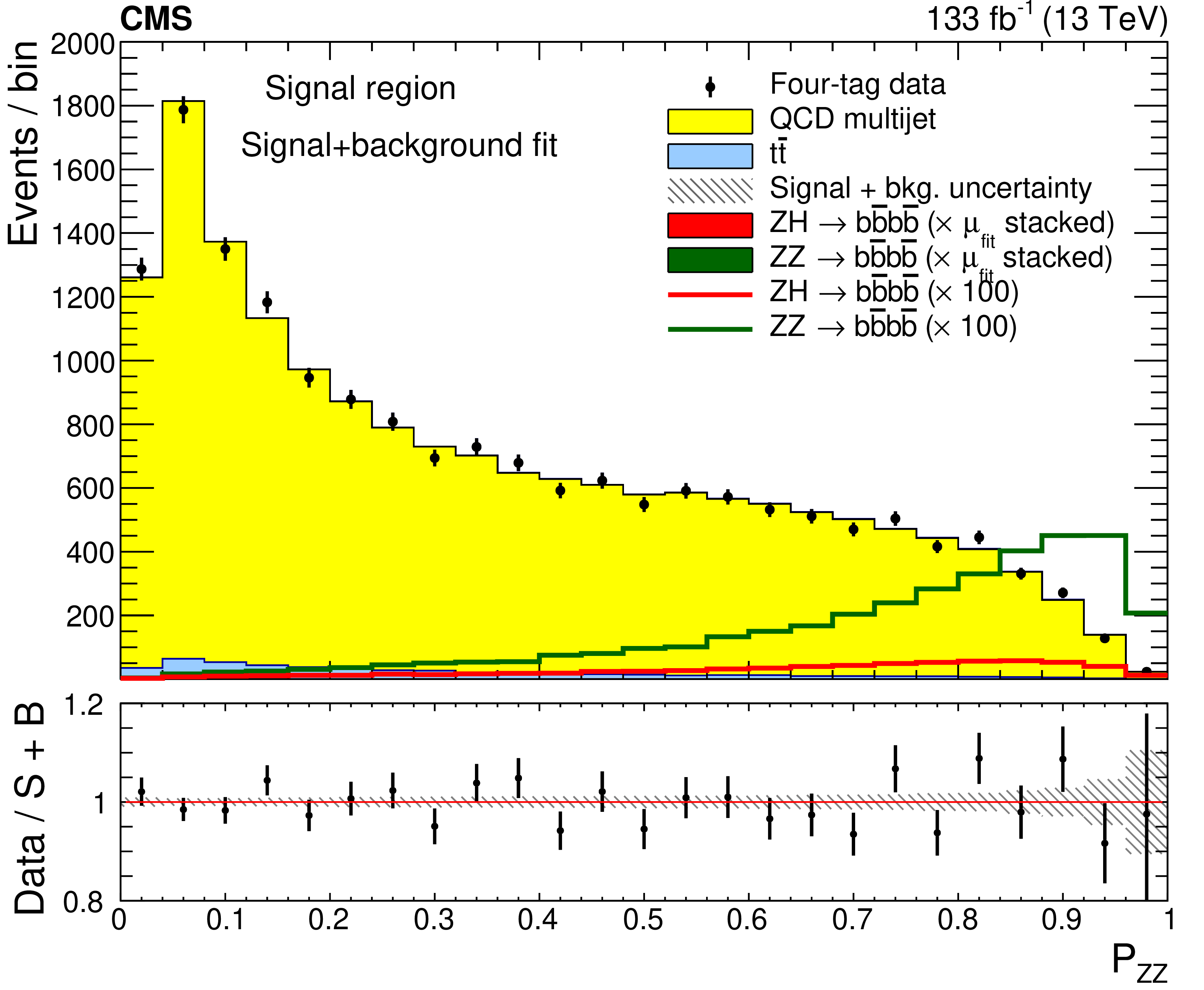
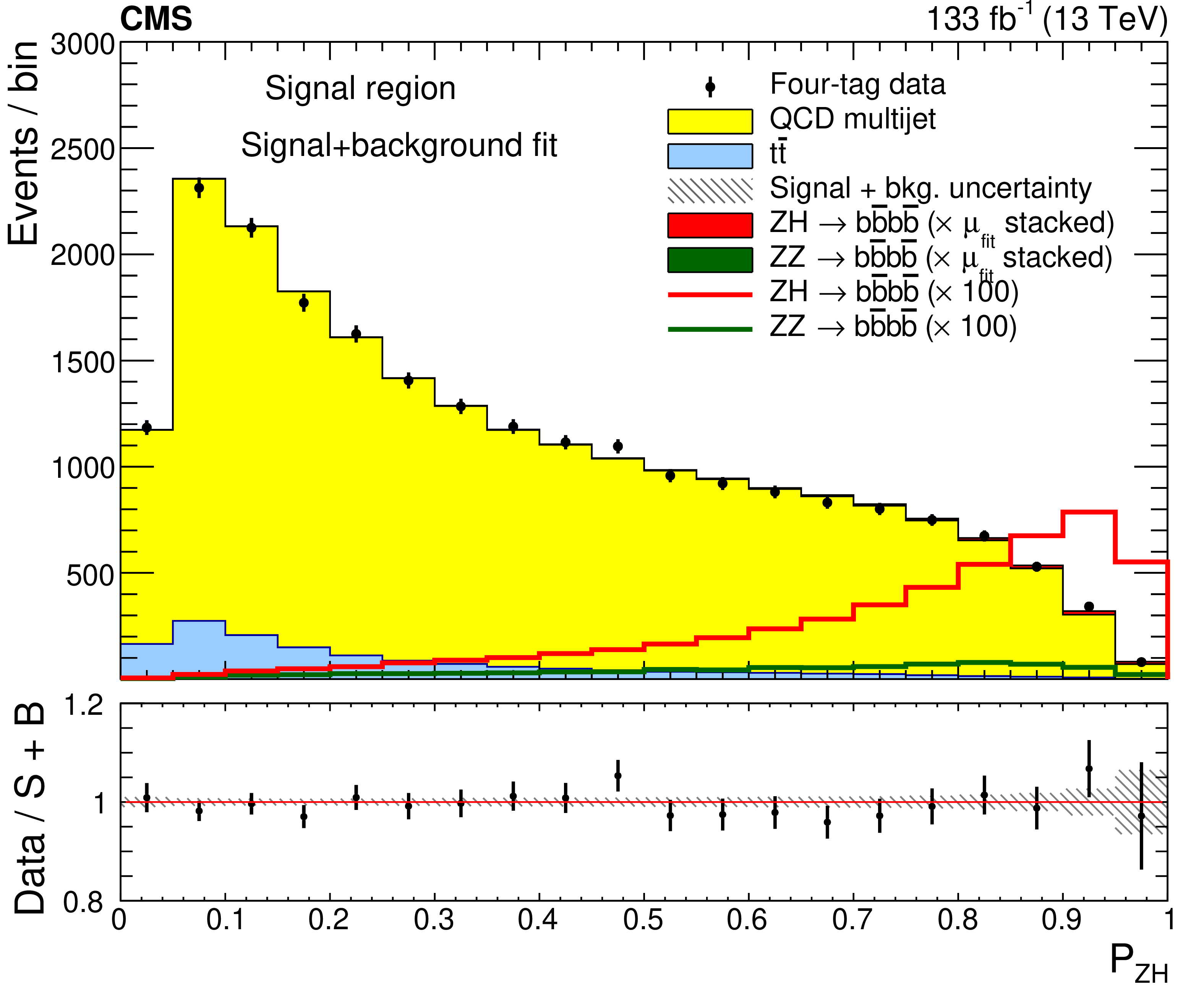
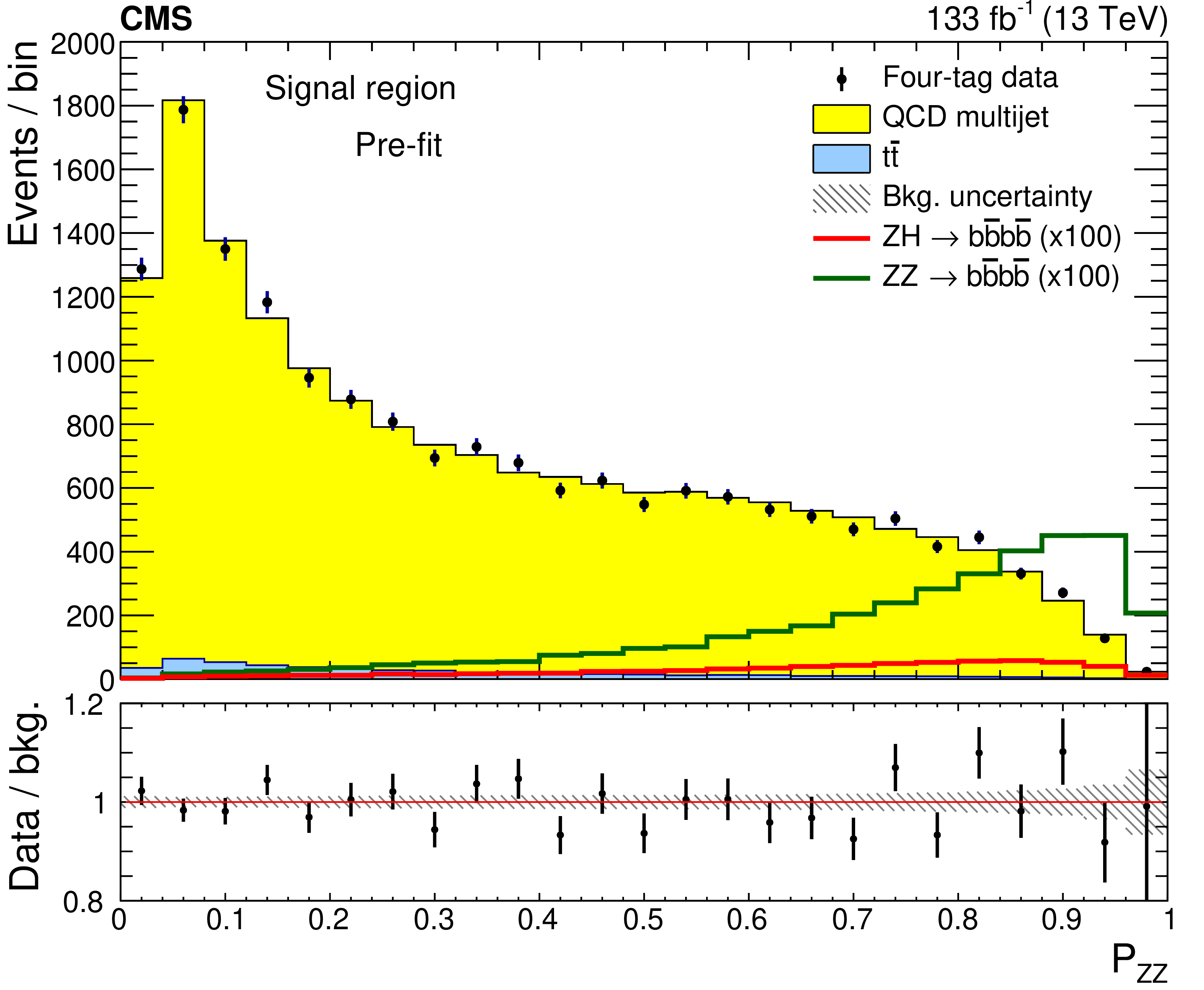
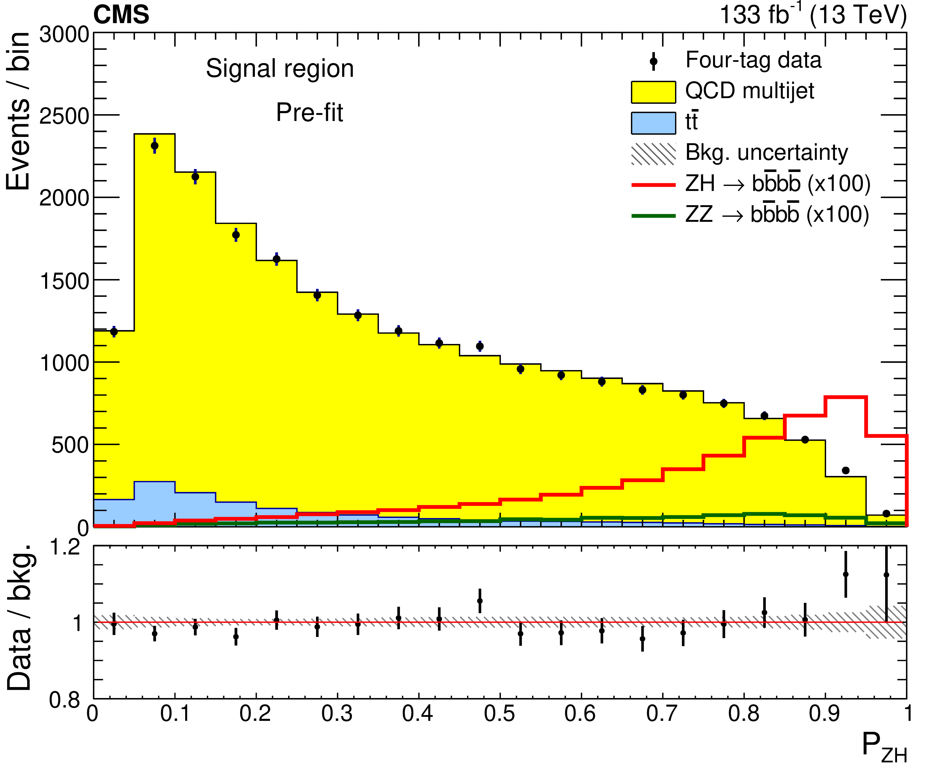
Figure 12:
Distributions of signal probabilities for ZZ (left) and ZH (right) channels (points), along with the post-fit QCD multijet (yellow region) plus $ \mathrm{t} \bar{\mathrm{t}} $ (blue region) distributions. The ZH and ZZ signal distributions scaled to the fitted signal strengths are shown, stacked on top of the background prediction. The expected ZH (red histograms) and ZZ (green histograms) signal channel distributions are also shown separately, multiplied by 100 for visibility. The lower panels display the ratio of the data to the result of the signal plus background fit, with the hatched area showing the uncertainty in the combined fit. |
png pdf |
Figure 12-a:
Distributions of signal probabilities for ZZ (left) and ZH (right) channels (points), along with the post-fit QCD multijet (yellow region) plus $ \mathrm{t} \bar{\mathrm{t}} $ (blue region) distributions. The ZH and ZZ signal distributions scaled to the fitted signal strengths are shown, stacked on top of the background prediction. The expected ZH (red histograms) and ZZ (green histograms) signal channel distributions are also shown separately, multiplied by 100 for visibility. The lower panels display the ratio of the data to the result of the signal plus background fit, with the hatched area showing the uncertainty in the combined fit. |
png pdf |
Figure 12-b:
Distributions of signal probabilities for ZZ (left) and ZH (right) channels (points), along with the post-fit QCD multijet (yellow region) plus $ \mathrm{t} \bar{\mathrm{t}} $ (blue region) distributions. The ZH and ZZ signal distributions scaled to the fitted signal strengths are shown, stacked on top of the background prediction. The expected ZH (red histograms) and ZZ (green histograms) signal channel distributions are also shown separately, multiplied by 100 for visibility. The lower panels display the ratio of the data to the result of the signal plus background fit, with the hatched area showing the uncertainty in the combined fit. |
| Tables | |
png pdf |
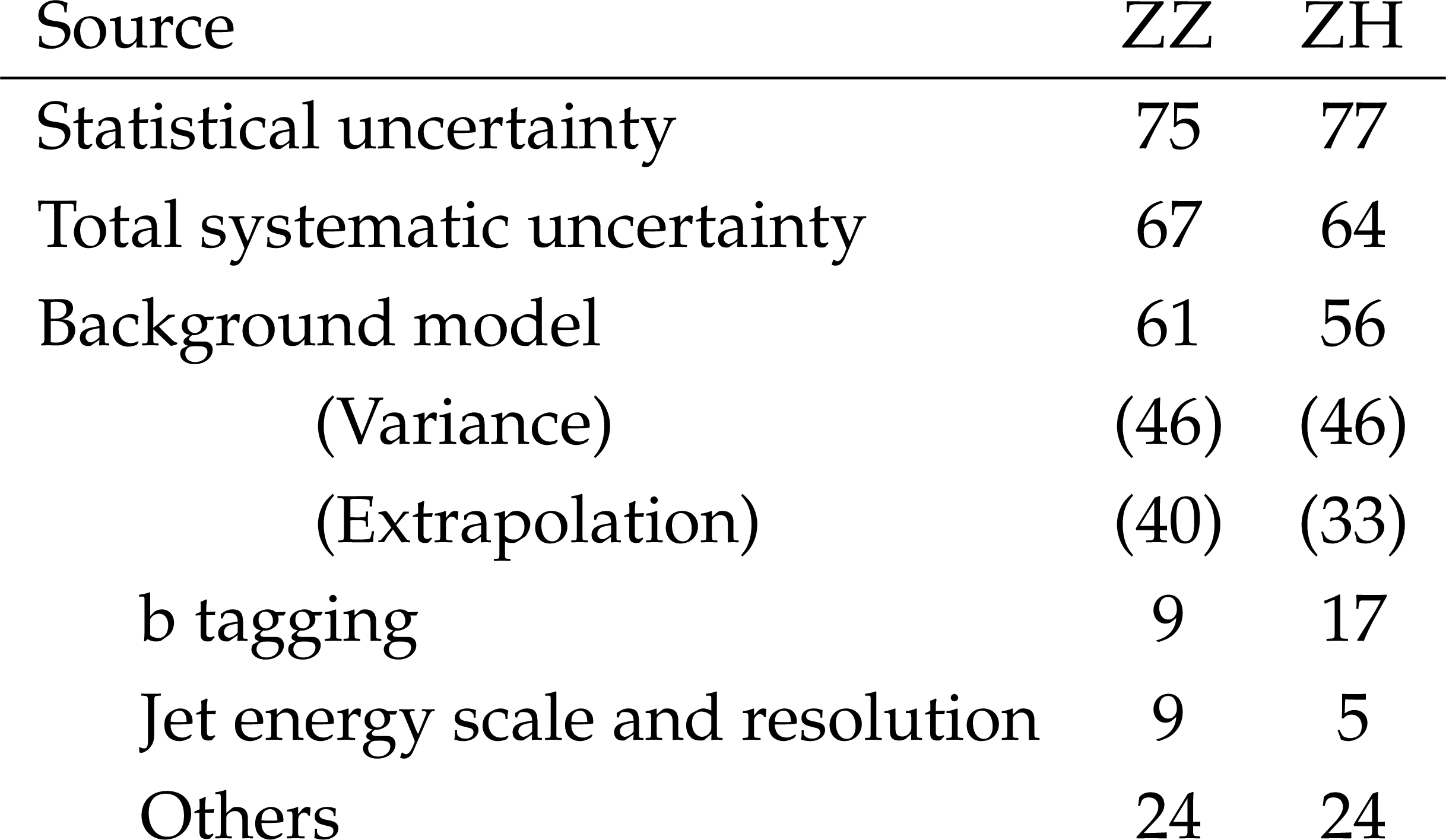
Table 1:
Summary of the relative uncertainties form the various sources in the measured signal strength, expressed as a percentage of the total uncertainty for the ZZ and ZH channels. The two uncertainties coming from the background modeling are given separately in parentheses, as well as their sum. The total systematic uncertainties shown include the effects of correlations. |

png pdf |
Table 2:
Expected and observed ZZ and ZH signal strengths and their corresponding 95% CL upper limits. The expected signal strengths and the corresponding expected upper limits shown in parentheses include only the statistical uncertainties. The upper limits are obtained from a fit to the SvB signal probabilities under the hypothesis of no $ \mathrm{Z}\mathrm{Z}\to 4\mathrm{b} $ or $ \mathrm{Z}\mathrm{H}\to 4\mathrm{b} $ signal. |
| Summary |
| A search for ZZ and ZH production in the 4b final state is presented. The search uses the full 2016--2018 data set of proton-proton collisions at a center-of-mass energy of 13 TeV recorded with the CMS detector at the LHC, corresponding to an integrated luminosity of 133 fb$ ^{-1} $. The analysis benefits from a multiclass multivariate classifier, which uses convolutions to solve the combinatoric jet pairing problem, and has been designed with an architecture customized to the 4b final state. The classifier is used both for signal-versus-background discrimination and for the derivation and validation of the background model. A novel technique for assessing the background modeling uncertainties, using a synthetic data sample, produced using a hemisphere mixing procedure, allows both the uncertainty in the background model and its variance to be measured with a precision better than the statistical uncertainties in the selected signal-region events. While these techniques are developed and demonstrated in the ZZ and $ \mathrm{Z}\mathrm{H} \to $ 4b searches, they are directly applicable to the $ \mathrm{H}\mathrm{H} \to 4\mathrm{b} $ analysis. The observed (expected) 95% CL upper limits on the $ \mathrm{Z}\mathrm{Z} \to 4\mathrm{b} $ and $ \mathrm{Z}\mathrm{H} \to 4\mathrm{b} $ production cross sections correspond to 3.8 (3.8) and 5.0 (2.9) times the standard model prediction, respectively. |
| Additional Figures | |

png pdf |
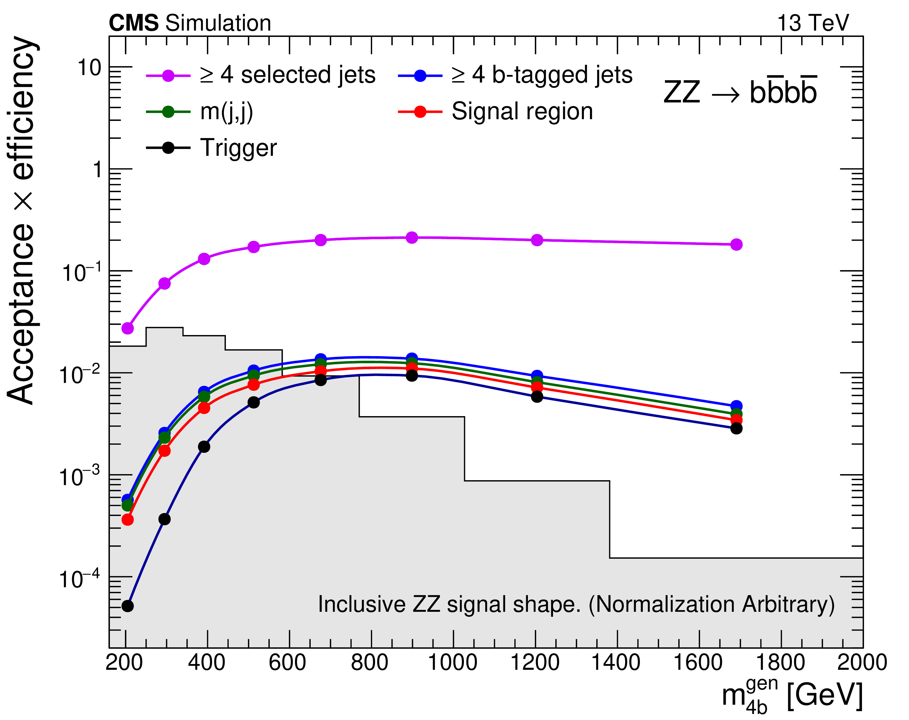
Additional Figure 1:
Acceptance times efficiency as a function of the generated four-body $ m_{4\mathrm{b}}^{\textrm{gen}} $ for the five different event selection requirements for simulated ZZ (left) and ZH (right). |

png pdf |
Additional Figure 1-a:
Acceptance times efficiency as a function of the generated four-body $ m_{4\mathrm{b}}^{\textrm{gen}} $ for the five different event selection requirements for simulated ZZ (left) and ZH (right). |

png pdf |
Additional Figure 1-b:
Acceptance times efficiency as a function of the generated four-body $ m_{4\mathrm{b}}^{\textrm{gen}} $ for the five different event selection requirements for simulated ZZ (left) and ZH (right). |

png pdf |
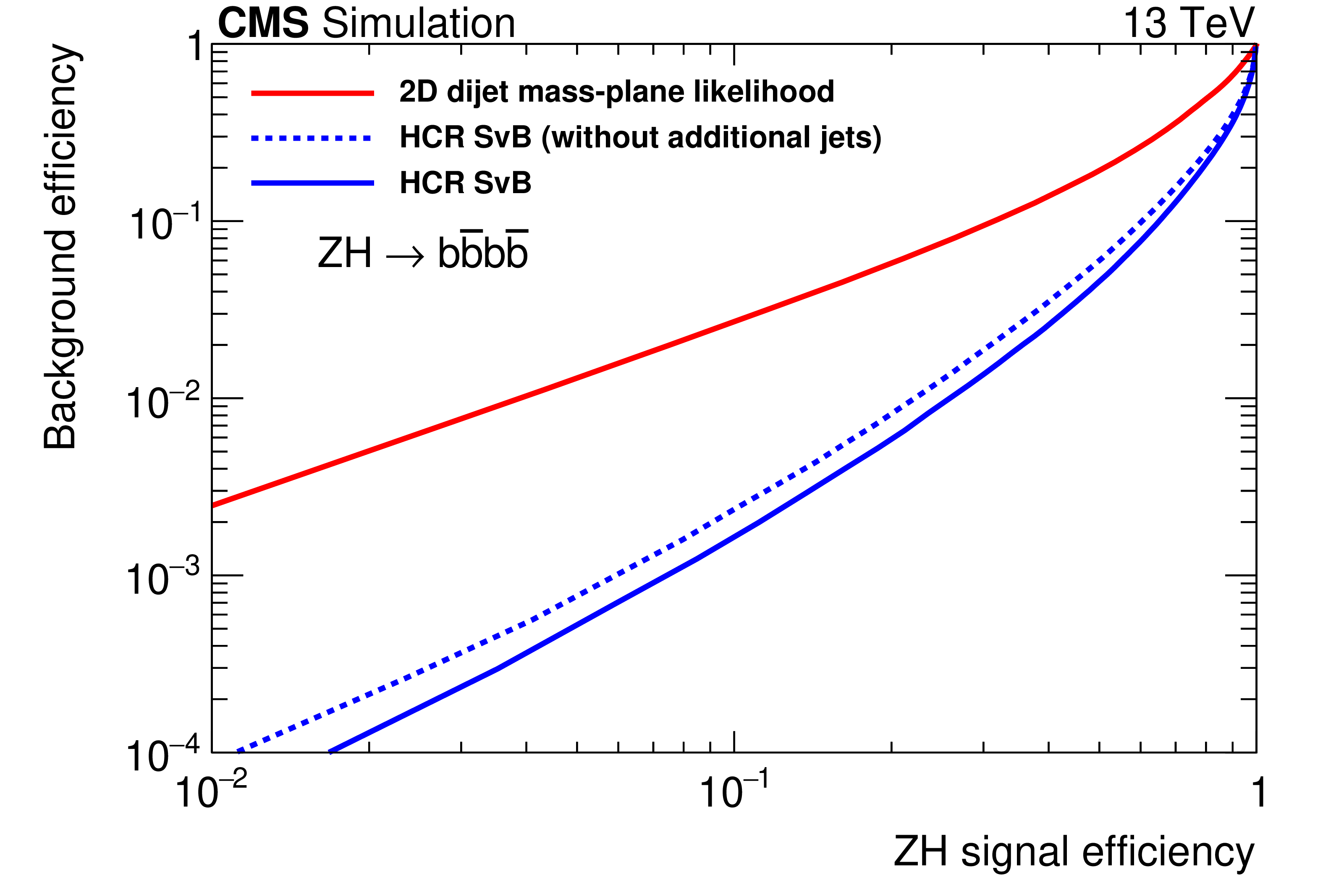
Additional Figure 2:
The ZZ (left) and ZH (right) signal efficiences from simulation versus the background efficiency for the nominal HCR SvB classier including additional jets, and for a simpler two-dimensional likelihood classifier using the two dijet invariant masses. A version of the HCR SvB classifier that does not include additional jets is also shown. |

png pdf |
Additional Figure 2-a:
The ZZ (left) and ZH (right) signal efficiences from simulation versus the background efficiency for the nominal HCR SvB classier including additional jets, and for a simpler two-dimensional likelihood classifier using the two dijet invariant masses. A version of the HCR SvB classifier that does not include additional jets is also shown. |
png pdf |
Additional Figure 2-b:
The ZZ (left) and ZH (right) signal efficiences from simulation versus the background efficiency for the nominal HCR SvB classier including additional jets, and for a simpler two-dimensional likelihood classifier using the two dijet invariant masses. A version of the HCR SvB classifier that does not include additional jets is also shown. |
png pdf |
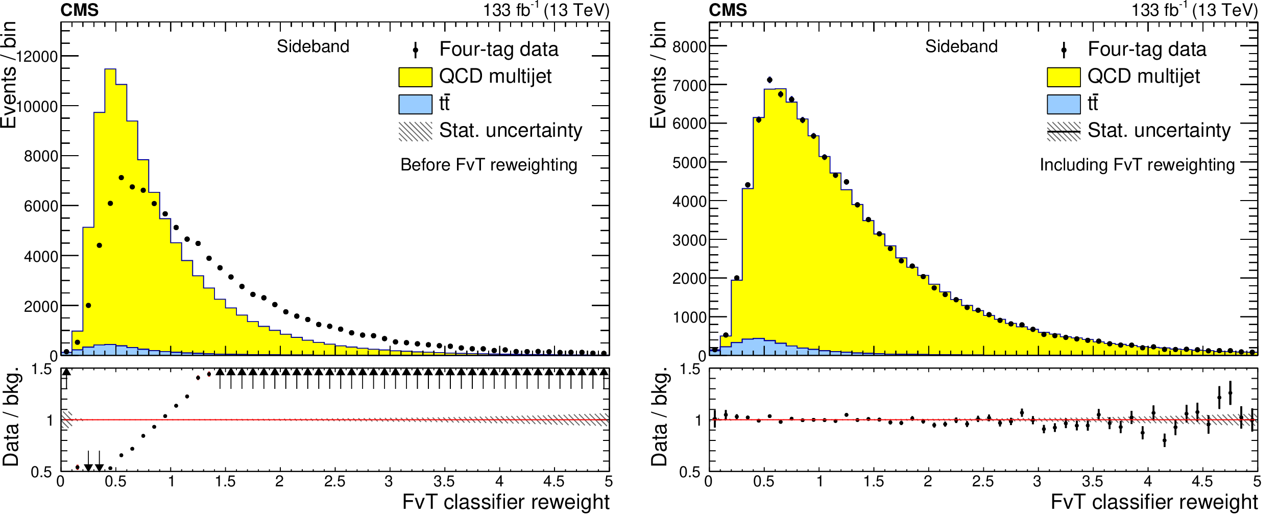
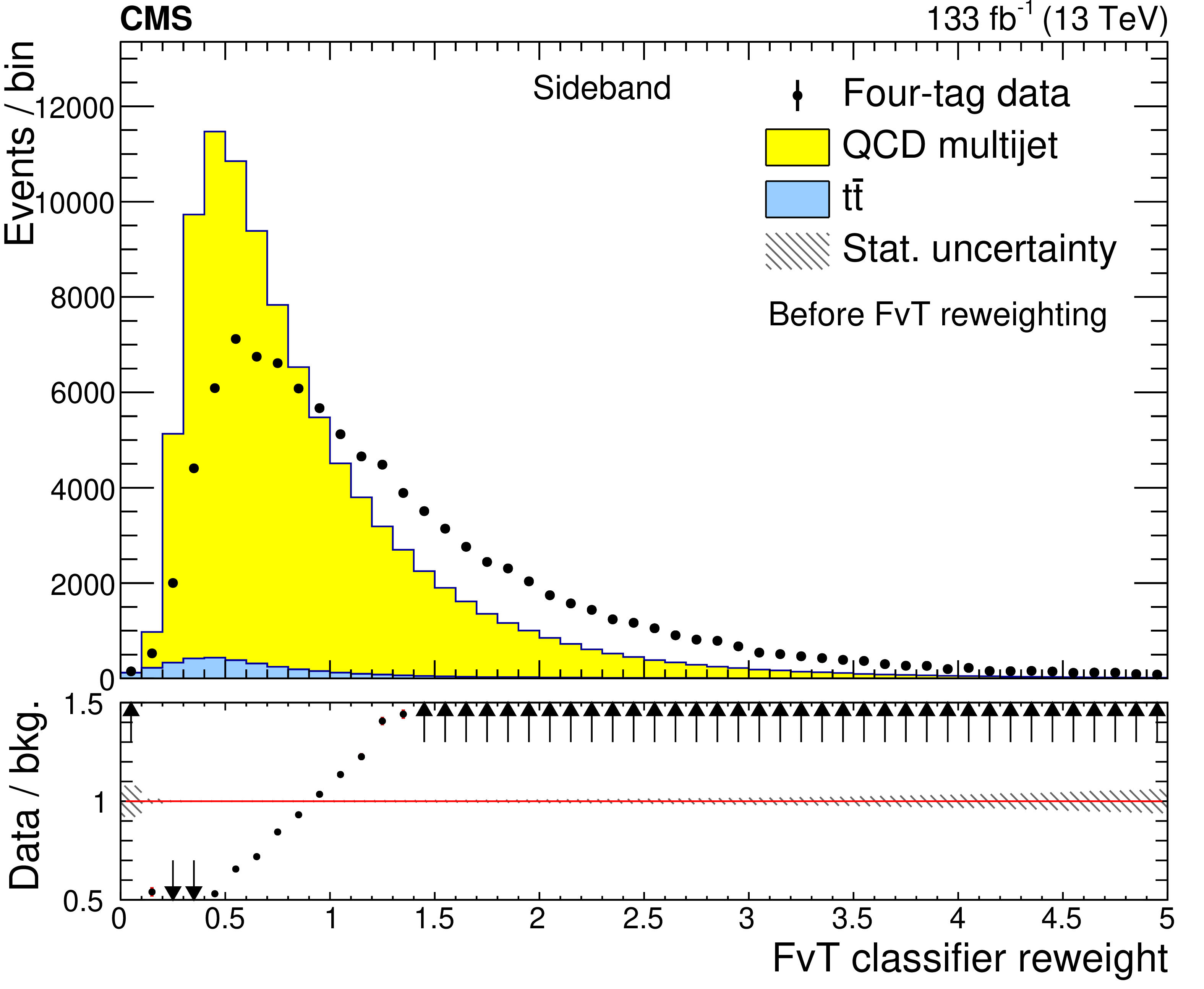
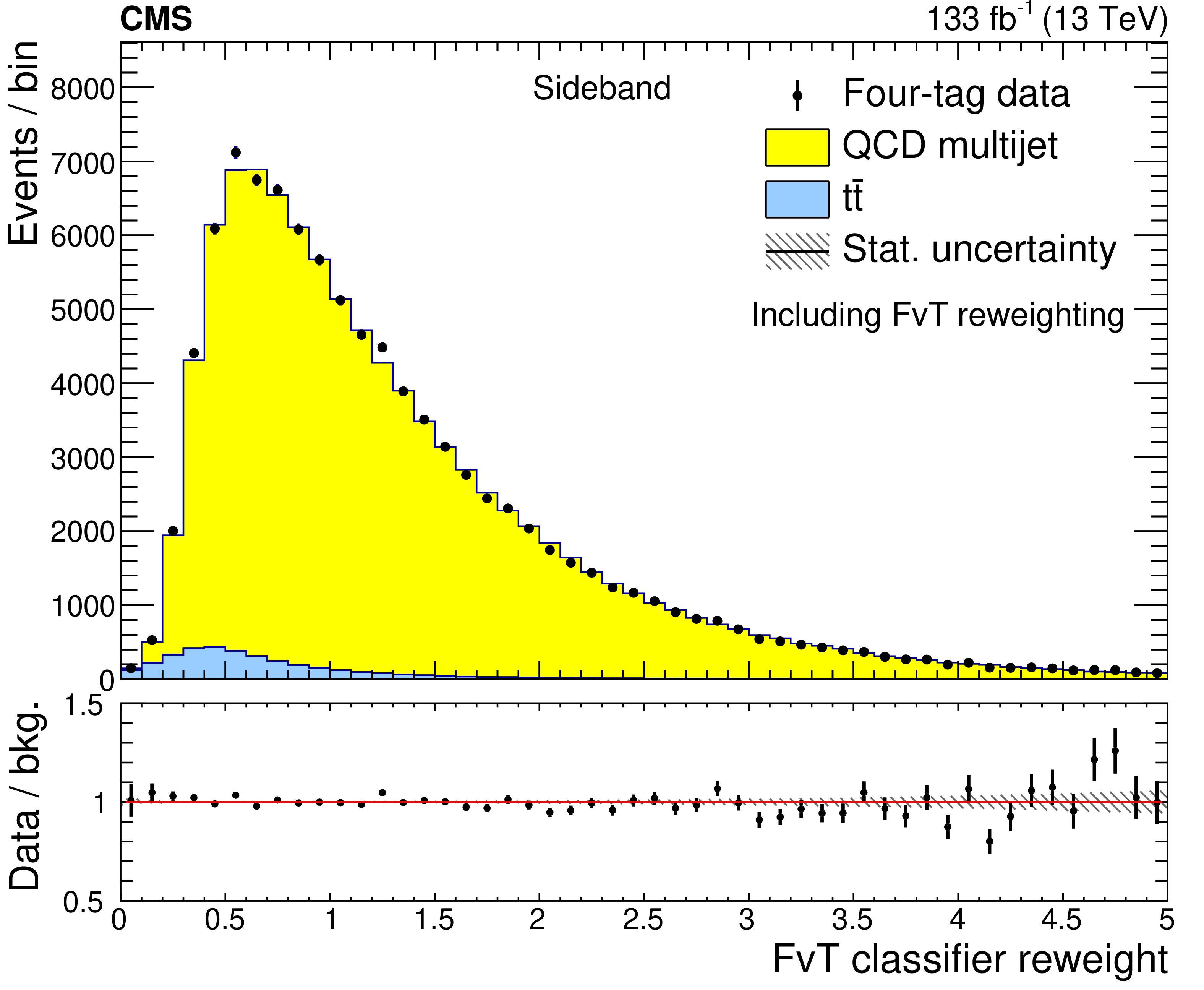
Additional Figure 3:
Distributions of the FvT classifier weights before (left) and after (right) applying the FvT corrections for the four-tag data (points), and the QCD multijet and $ \mathrm{t} \bar{\mathrm{t}} $ backgrounds (yellow and blue distributions, respectively). The lower panels display the ratio of the data to the sum of the QCD multijet and $ \mathrm{t} \bar{\mathrm{t}} $ distributions. The hatched region represents the uncertainties in the background. |
png pdf |
Additional Figure 3-a:
Distributions of the FvT classifier weights before (left) and after (right) applying the FvT corrections for the four-tag data (points), and the QCD multijet and $ \mathrm{t} \bar{\mathrm{t}} $ backgrounds (yellow and blue distributions, respectively). The lower panels display the ratio of the data to the sum of the QCD multijet and $ \mathrm{t} \bar{\mathrm{t}} $ distributions. The hatched region represents the uncertainties in the background. |
png pdf |
Additional Figure 3-b:
Distributions of the FvT classifier weights before (left) and after (right) applying the FvT corrections for the four-tag data (points), and the QCD multijet and $ \mathrm{t} \bar{\mathrm{t}} $ backgrounds (yellow and blue distributions, respectively). The lower panels display the ratio of the data to the sum of the QCD multijet and $ \mathrm{t} \bar{\mathrm{t}} $ distributions. The hatched region represents the uncertainties in the background. |

png pdf |
Additional Figure 4:
The SvB signal probability distributions in the ZZ SR for one of the mixed data samples (left) and the average of the fifteen mixed samples (right). The points show the mixed model results, the QCD multijet and $ \mathrm{t} \bar{\mathrm{t}} $ background distributions are shown by the yellow and blue regions, respectively. The expected signal distributions for ZZ and ZH are shown by the green and red histograms, multiplied by 100. The lower panels display the ratio of the mixed sample distribution to the sum of the QCD multijet and $ \mathrm{t} \bar{\mathrm{t}} $ distributions. The hatched area gives the statistical uncertainty in the ratio. |

png pdf |
Additional Figure 4-a:
The SvB signal probability distributions in the ZZ SR for one of the mixed data samples (left) and the average of the fifteen mixed samples (right). The points show the mixed model results, the QCD multijet and $ \mathrm{t} \bar{\mathrm{t}} $ background distributions are shown by the yellow and blue regions, respectively. The expected signal distributions for ZZ and ZH are shown by the green and red histograms, multiplied by 100. The lower panels display the ratio of the mixed sample distribution to the sum of the QCD multijet and $ \mathrm{t} \bar{\mathrm{t}} $ distributions. The hatched area gives the statistical uncertainty in the ratio. |

png pdf |
Additional Figure 4-b:
The SvB signal probability distributions in the ZZ SR for one of the mixed data samples (left) and the average of the fifteen mixed samples (right). The points show the mixed model results, the QCD multijet and $ \mathrm{t} \bar{\mathrm{t}} $ background distributions are shown by the yellow and blue regions, respectively. The expected signal distributions for ZZ and ZH are shown by the green and red histograms, multiplied by 100. The lower panels display the ratio of the mixed sample distribution to the sum of the QCD multijet and $ \mathrm{t} \bar{\mathrm{t}} $ distributions. The hatched area gives the statistical uncertainty in the ratio. |
png pdf |
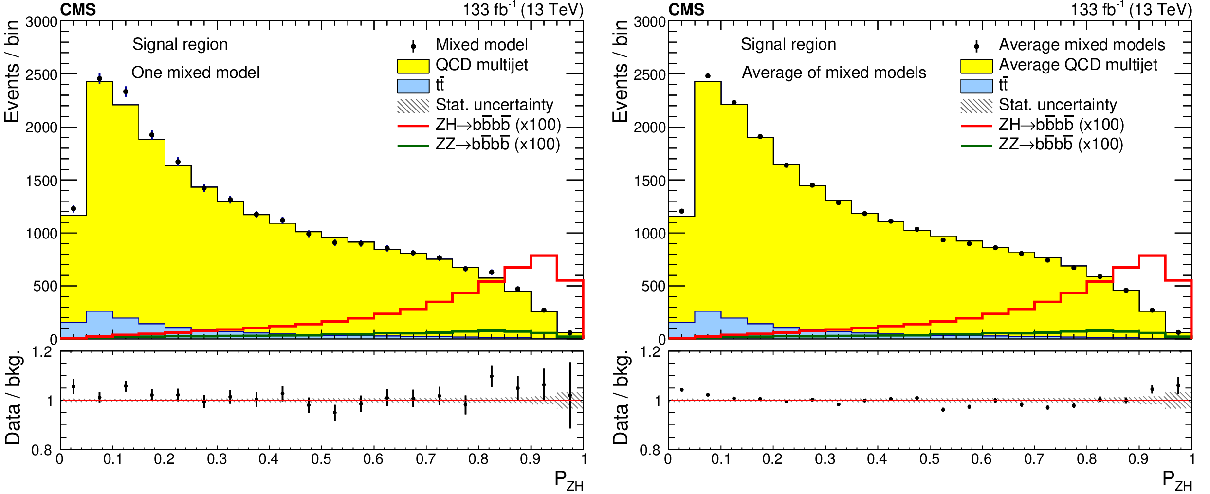
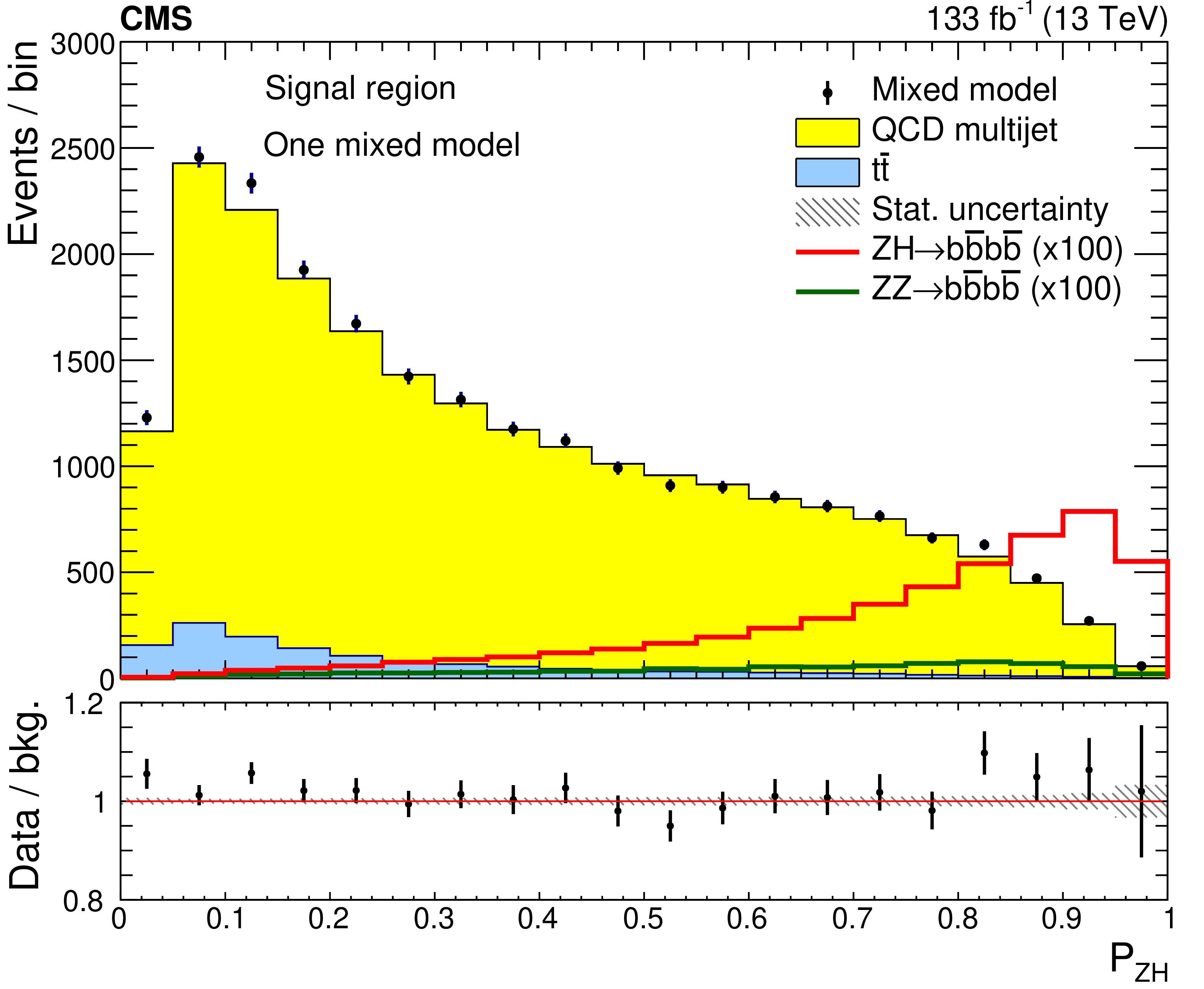
Additional Figure 5:
The SvB signal probability distributions in the ZH SR for one of the mixed data samples (left) and the average of the fifteen mixed samples (right). The points show the mixed model results, the QCD multijet and $ \mathrm{t} \bar{\mathrm{t}} $ background distributions are shown by the yellow and blue regions, respectively. The expected signal distributions for ZZ and ZH are shown by the green and red histograms, multiplied by 100. The lower panels display the ratio of the mixed sample distribution to the sum of the QCD multijet and $ \mathrm{t} \bar{\mathrm{t}} $ distributions. The hatched area gives the statistical uncertainty in the ratio. |
png pdf |
Additional Figure 5-a:
The SvB signal probability distributions in the ZH SR for one of the mixed data samples (left) and the average of the fifteen mixed samples (right). The points show the mixed model results, the QCD multijet and $ \mathrm{t} \bar{\mathrm{t}} $ background distributions are shown by the yellow and blue regions, respectively. The expected signal distributions for ZZ and ZH are shown by the green and red histograms, multiplied by 100. The lower panels display the ratio of the mixed sample distribution to the sum of the QCD multijet and $ \mathrm{t} \bar{\mathrm{t}} $ distributions. The hatched area gives the statistical uncertainty in the ratio. |

png pdf |
Additional Figure 5-b:
The SvB signal probability distributions in the ZH SR for one of the mixed data samples (left) and the average of the fifteen mixed samples (right). The points show the mixed model results, the QCD multijet and $ \mathrm{t} \bar{\mathrm{t}} $ background distributions are shown by the yellow and blue regions, respectively. The expected signal distributions for ZZ and ZH are shown by the green and red histograms, multiplied by 100. The lower panels display the ratio of the mixed sample distribution to the sum of the QCD multijet and $ \mathrm{t} \bar{\mathrm{t}} $ distributions. The hatched area gives the statistical uncertainty in the ratio. |
png pdf |
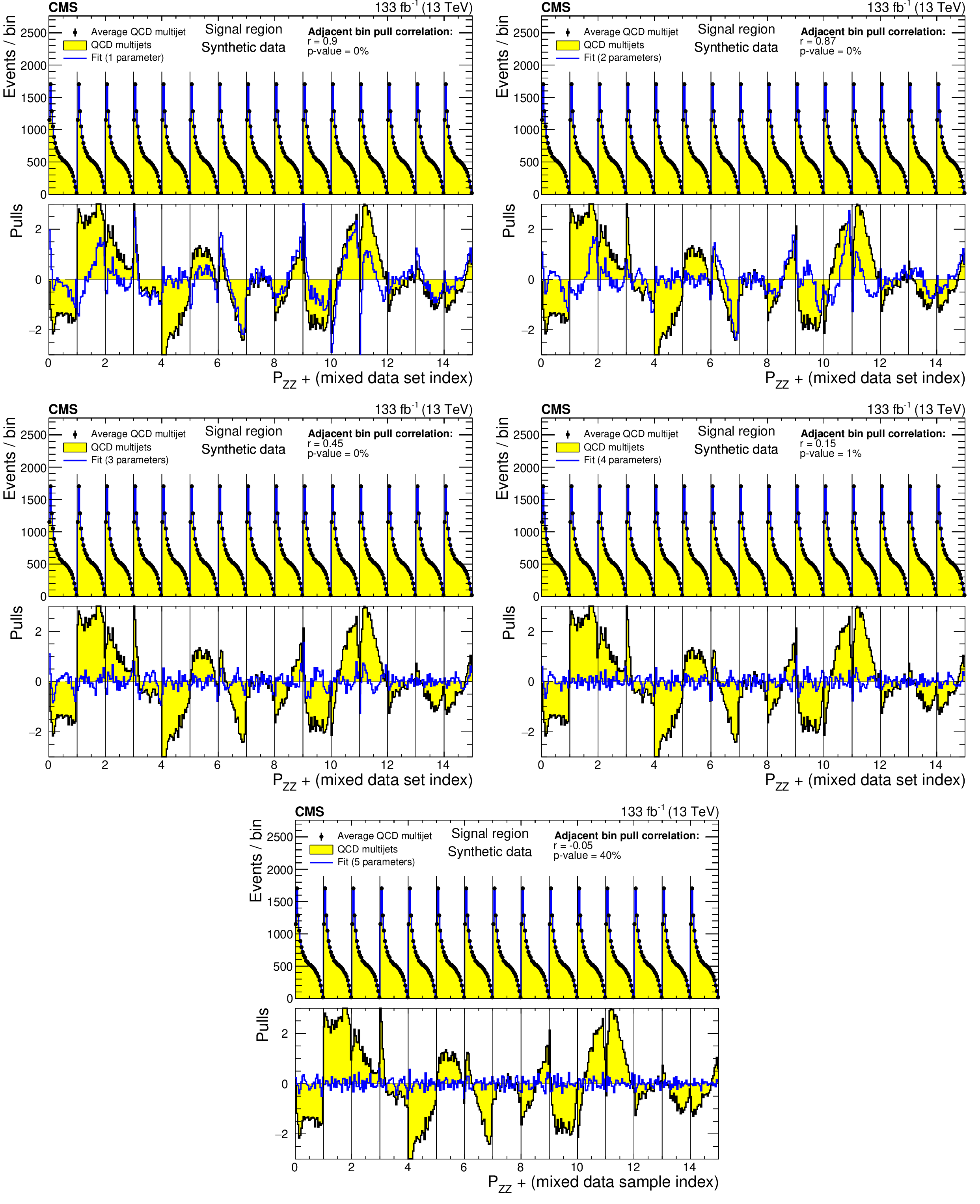
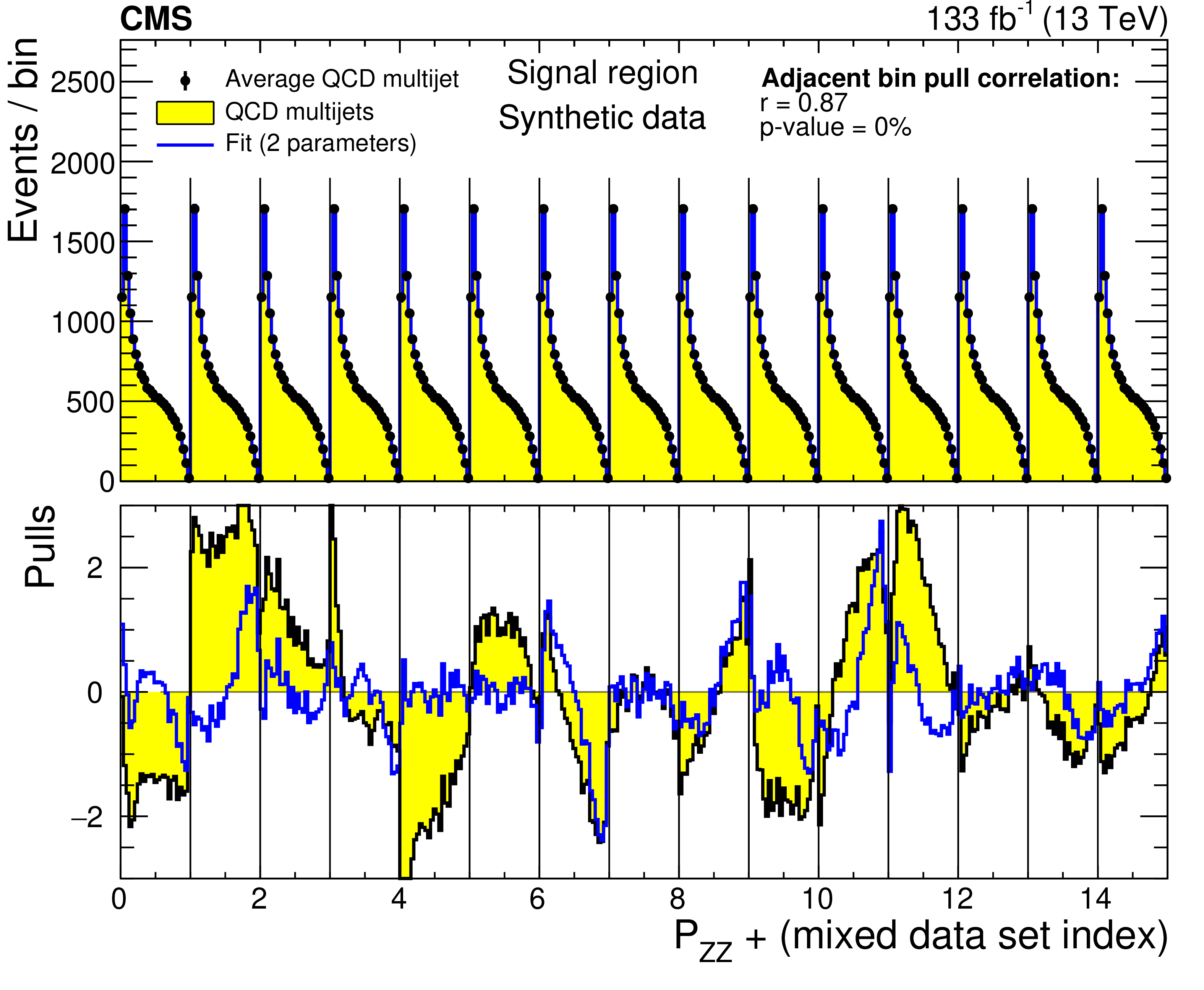
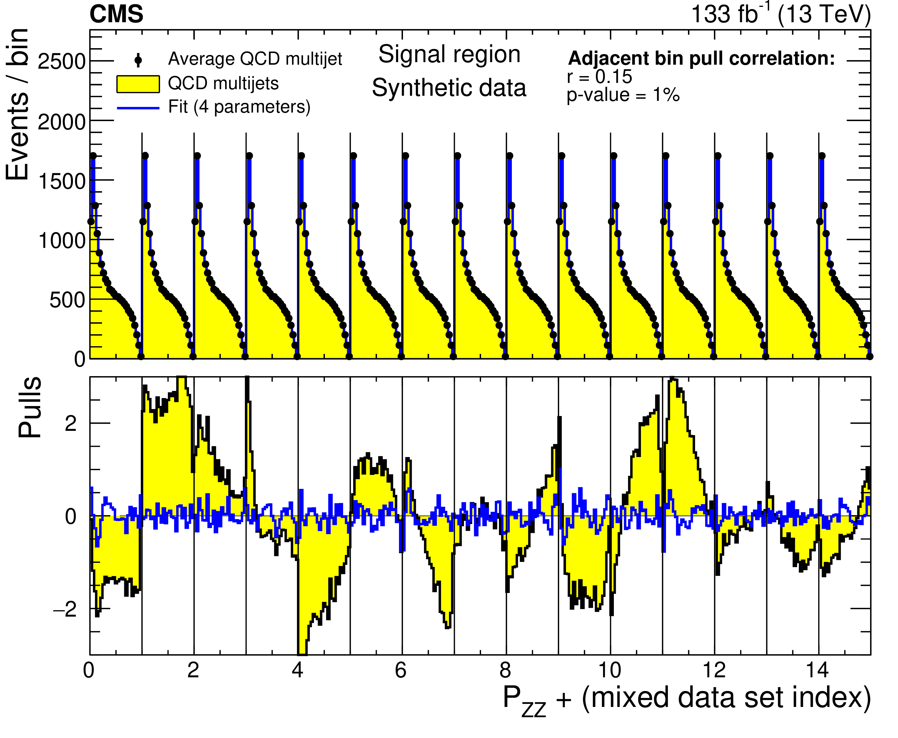
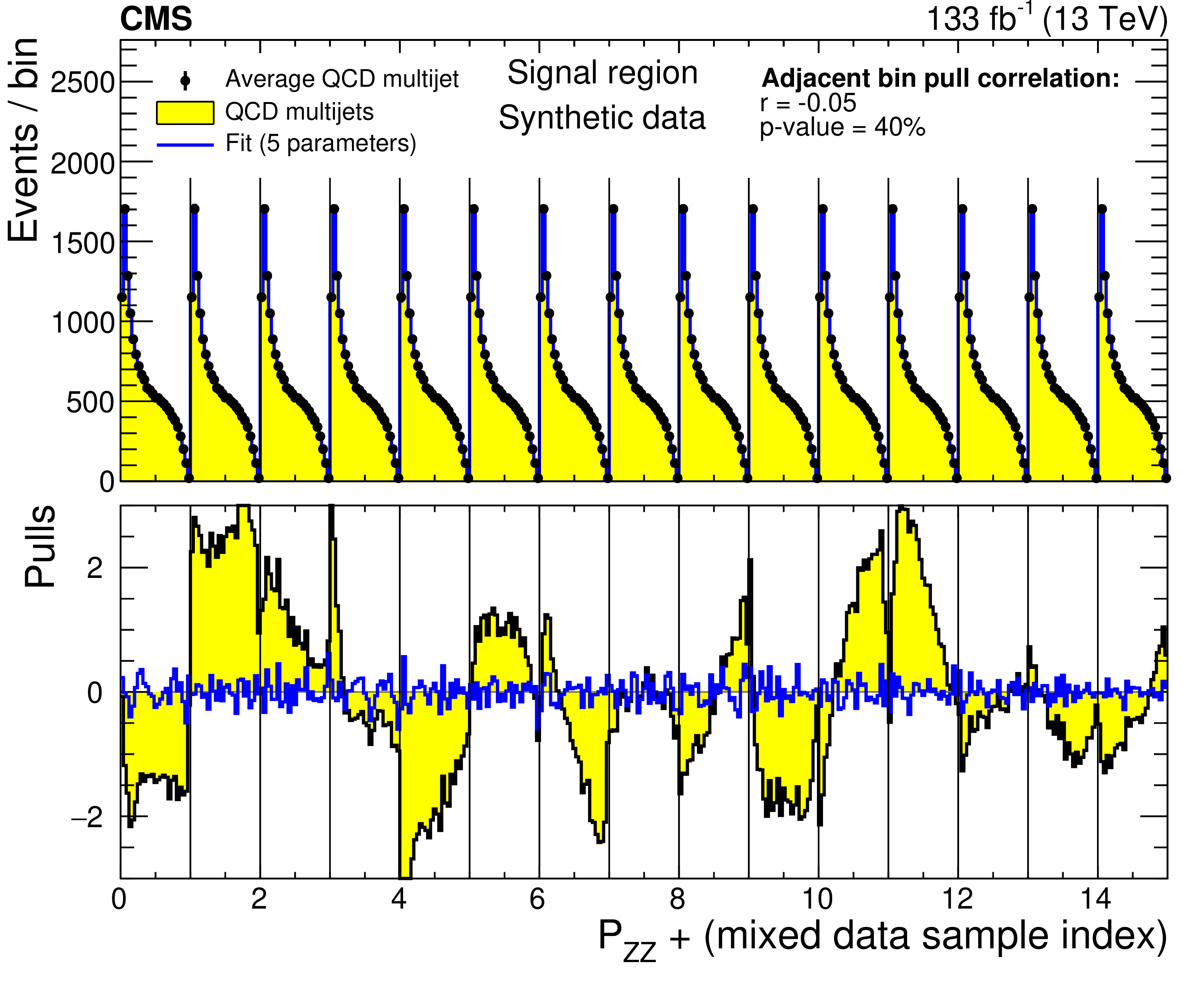
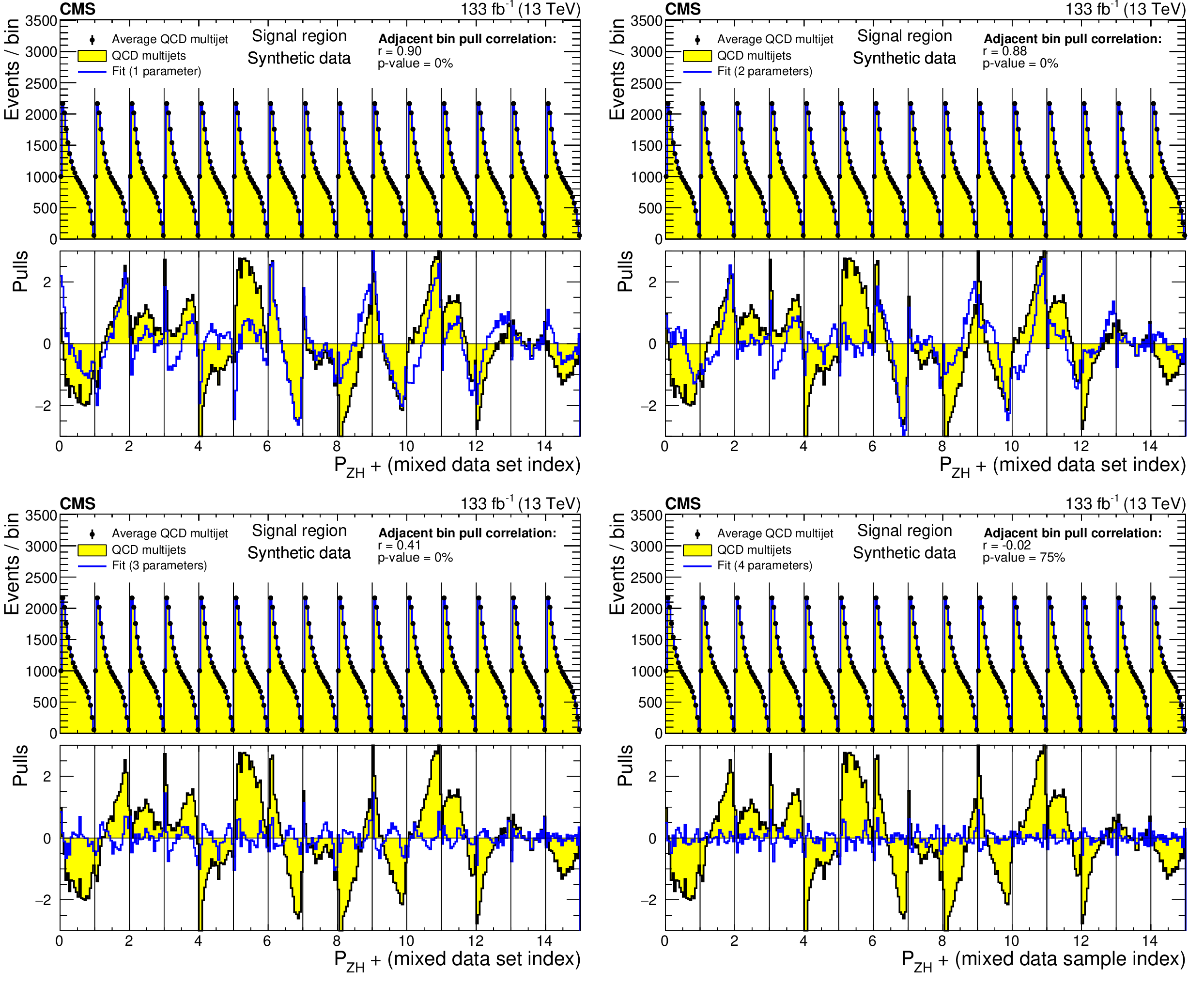
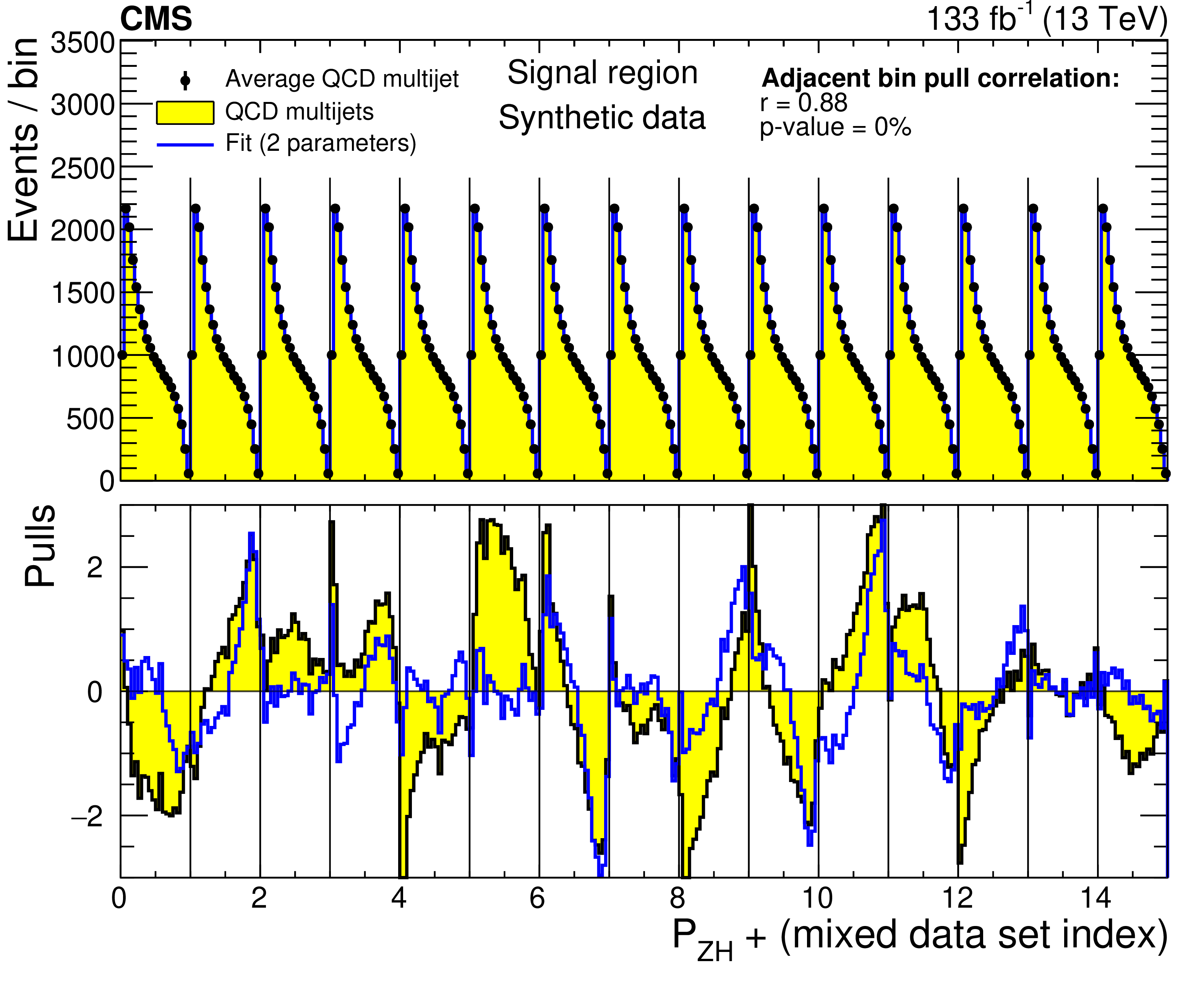
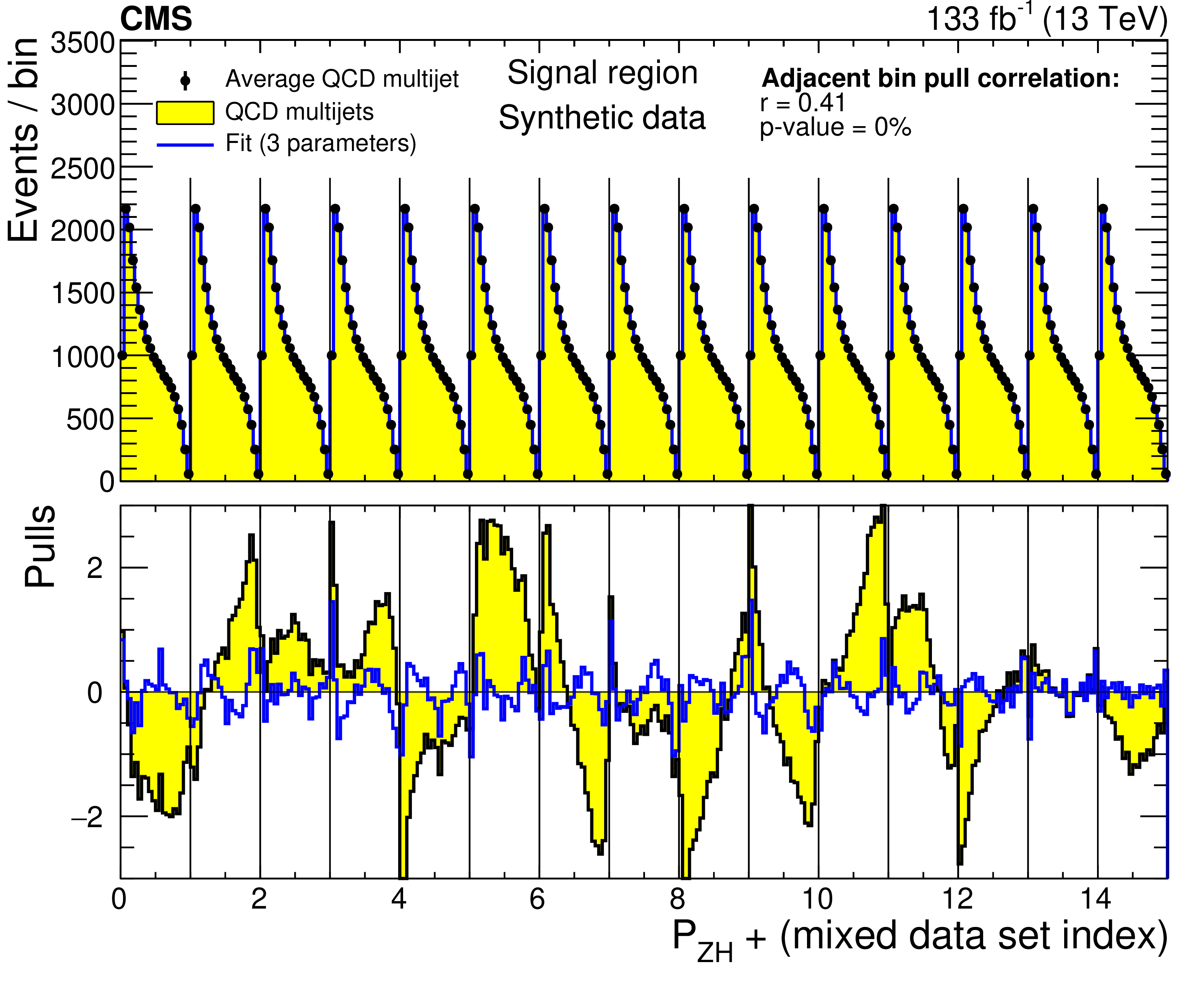
Additional Figure 6:
The predicted QCD multijet ZZ SvB probability distributions for each of the 15 mixed data sample SRs (yellow regions). The distribution from each mixed data sample is offset by the data sample index number. The black points give the average of the 15 data samples. The solid blue curves show a fit to the individual distributions using an increasing number of basis functions from one in the upper left plot to five in the lowest plot. The lower panels show the pulls before (yellow histogram) and after (blue histogram) adding the basis corrections. The correlation coefficient (r) for a fit testing for correlations is given in the legend, along with the p-value used to test for lack of correlation. Basis functions are added until the p-value is greater than 5%. |

png pdf |
Additional Figure 6-a:
The predicted QCD multijet ZZ SvB probability distributions for each of the 15 mixed data sample SRs (yellow regions). The distribution from each mixed data sample is offset by the data sample index number. The black points give the average of the 15 data samples. The solid blue curves show a fit to the individual distributions using an increasing number of basis functions from one in the upper left plot to five in the lowest plot. The lower panels show the pulls before (yellow histogram) and after (blue histogram) adding the basis corrections. The correlation coefficient (r) for a fit testing for correlations is given in the legend, along with the p-value used to test for lack of correlation. Basis functions are added until the p-value is greater than 5%. |
png pdf |
Additional Figure 6-b:
The predicted QCD multijet ZZ SvB probability distributions for each of the 15 mixed data sample SRs (yellow regions). The distribution from each mixed data sample is offset by the data sample index number. The black points give the average of the 15 data samples. The solid blue curves show a fit to the individual distributions using an increasing number of basis functions from one in the upper left plot to five in the lowest plot. The lower panels show the pulls before (yellow histogram) and after (blue histogram) adding the basis corrections. The correlation coefficient (r) for a fit testing for correlations is given in the legend, along with the p-value used to test for lack of correlation. Basis functions are added until the p-value is greater than 5%. |

png pdf |
Additional Figure 6-c:
The predicted QCD multijet ZZ SvB probability distributions for each of the 15 mixed data sample SRs (yellow regions). The distribution from each mixed data sample is offset by the data sample index number. The black points give the average of the 15 data samples. The solid blue curves show a fit to the individual distributions using an increasing number of basis functions from one in the upper left plot to five in the lowest plot. The lower panels show the pulls before (yellow histogram) and after (blue histogram) adding the basis corrections. The correlation coefficient (r) for a fit testing for correlations is given in the legend, along with the p-value used to test for lack of correlation. Basis functions are added until the p-value is greater than 5%. |
png pdf |
Additional Figure 6-d:
The predicted QCD multijet ZZ SvB probability distributions for each of the 15 mixed data sample SRs (yellow regions). The distribution from each mixed data sample is offset by the data sample index number. The black points give the average of the 15 data samples. The solid blue curves show a fit to the individual distributions using an increasing number of basis functions from one in the upper left plot to five in the lowest plot. The lower panels show the pulls before (yellow histogram) and after (blue histogram) adding the basis corrections. The correlation coefficient (r) for a fit testing for correlations is given in the legend, along with the p-value used to test for lack of correlation. Basis functions are added until the p-value is greater than 5%. |
png pdf |
Additional Figure 6-e:
The predicted QCD multijet ZZ SvB probability distributions for each of the 15 mixed data sample SRs (yellow regions). The distribution from each mixed data sample is offset by the data sample index number. The black points give the average of the 15 data samples. The solid blue curves show a fit to the individual distributions using an increasing number of basis functions from one in the upper left plot to five in the lowest plot. The lower panels show the pulls before (yellow histogram) and after (blue histogram) adding the basis corrections. The correlation coefficient (r) for a fit testing for correlations is given in the legend, along with the p-value used to test for lack of correlation. Basis functions are added until the p-value is greater than 5%. |
png pdf |
Additional Figure 7:
The predicted QCD multijet ZH SvB probability distributions for each of the 15 mixed data sample SRs (yellow regions). The distribution from each mixed data sample is offset by the data sample index number. The black points give the average of the 15 data samples. The solid blue curves show a fit to the individual distributions using an increasing number of basis functions from one in the upper left plot to five in the lowest plot. The lower panels show the pulls before (yellow histogram) and after (blue histogram) adding the basis corrections. The correlation coefficient (r) for a fit testing for correlations is given in the legend, along with the p-value used to test for lack of correlation. Basis functions are added until the p-value is greater than 5%. |

png pdf |
Additional Figure 7-a:
The predicted QCD multijet ZH SvB probability distributions for each of the 15 mixed data sample SRs (yellow regions). The distribution from each mixed data sample is offset by the data sample index number. The black points give the average of the 15 data samples. The solid blue curves show a fit to the individual distributions using an increasing number of basis functions from one in the upper left plot to five in the lowest plot. The lower panels show the pulls before (yellow histogram) and after (blue histogram) adding the basis corrections. The correlation coefficient (r) for a fit testing for correlations is given in the legend, along with the p-value used to test for lack of correlation. Basis functions are added until the p-value is greater than 5%. |
png pdf |
Additional Figure 7-b:
The predicted QCD multijet ZH SvB probability distributions for each of the 15 mixed data sample SRs (yellow regions). The distribution from each mixed data sample is offset by the data sample index number. The black points give the average of the 15 data samples. The solid blue curves show a fit to the individual distributions using an increasing number of basis functions from one in the upper left plot to five in the lowest plot. The lower panels show the pulls before (yellow histogram) and after (blue histogram) adding the basis corrections. The correlation coefficient (r) for a fit testing for correlations is given in the legend, along with the p-value used to test for lack of correlation. Basis functions are added until the p-value is greater than 5%. |
png pdf |
Additional Figure 7-c:
The predicted QCD multijet ZH SvB probability distributions for each of the 15 mixed data sample SRs (yellow regions). The distribution from each mixed data sample is offset by the data sample index number. The black points give the average of the 15 data samples. The solid blue curves show a fit to the individual distributions using an increasing number of basis functions from one in the upper left plot to five in the lowest plot. The lower panels show the pulls before (yellow histogram) and after (blue histogram) adding the basis corrections. The correlation coefficient (r) for a fit testing for correlations is given in the legend, along with the p-value used to test for lack of correlation. Basis functions are added until the p-value is greater than 5%. |

png pdf |
Additional Figure 7-d:
The predicted QCD multijet ZH SvB probability distributions for each of the 15 mixed data sample SRs (yellow regions). The distribution from each mixed data sample is offset by the data sample index number. The black points give the average of the 15 data samples. The solid blue curves show a fit to the individual distributions using an increasing number of basis functions from one in the upper left plot to five in the lowest plot. The lower panels show the pulls before (yellow histogram) and after (blue histogram) adding the basis corrections. The correlation coefficient (r) for a fit testing for correlations is given in the legend, along with the p-value used to test for lack of correlation. Basis functions are added until the p-value is greater than 5%. |

png pdf |
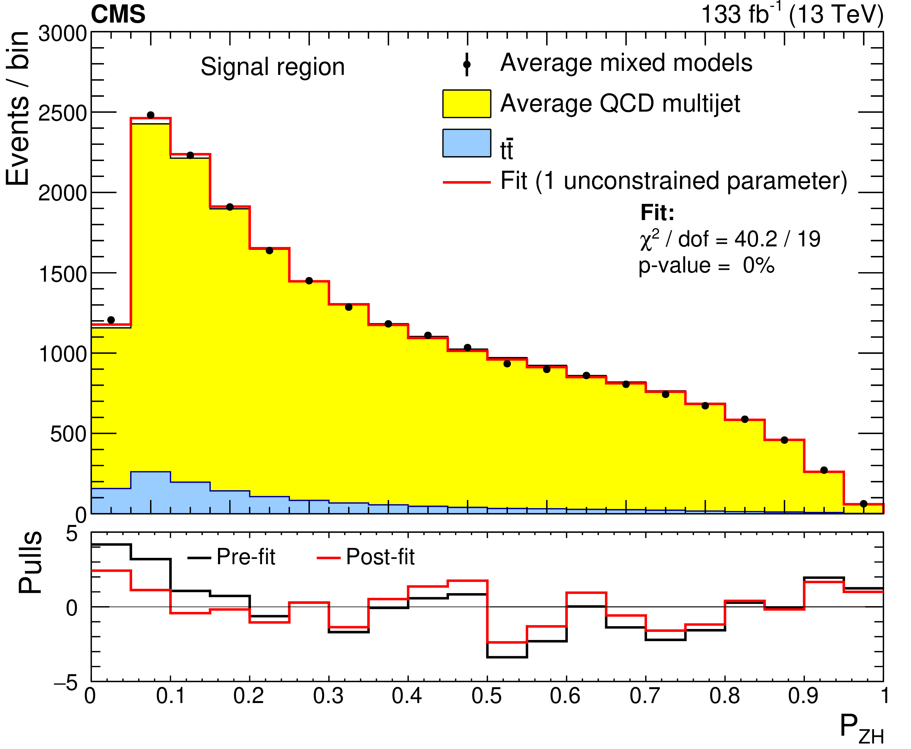
Additional Figure 8:
Distributions of the ZH signal probability for the average observed SR yields from the mixed models. The yellow and blue regions give the distributions of the average of the QCD multijet models and the $ \mathrm{t} \bar{\mathrm{t}} $ simulation, respectively. The red histogram displays the post-fit results of the data fit to the background model with 0 (left) and 1 unconstrained parameter (right) in the fit. The $ \chi^2 $ / dof and the p-value from the fit are shown in the legend. The lower panels give the pre- (blue histograms) and post-fit (red histograms) pulls. |

png pdf |
Additional Figure 8-a:
Distributions of the ZH signal probability for the average observed SR yields from the mixed models. The yellow and blue regions give the distributions of the average of the QCD multijet models and the $ \mathrm{t} \bar{\mathrm{t}} $ simulation, respectively. The red histogram displays the post-fit results of the data fit to the background model with 0 (left) and 1 unconstrained parameter (right) in the fit. The $ \chi^2 $ / dof and the p-value from the fit are shown in the legend. The lower panels give the pre- (blue histograms) and post-fit (red histograms) pulls. |
png pdf |
Additional Figure 8-b:
Distributions of the ZH signal probability for the average observed SR yields from the mixed models. The yellow and blue regions give the distributions of the average of the QCD multijet models and the $ \mathrm{t} \bar{\mathrm{t}} $ simulation, respectively. The red histogram displays the post-fit results of the data fit to the background model with 0 (left) and 1 unconstrained parameter (right) in the fit. The $ \chi^2 $ / dof and the p-value from the fit are shown in the legend. The lower panels give the pre- (blue histograms) and post-fit (red histograms) pulls. |

png pdf |
Additional Figure 9:
The pre-fit signal SvB signal probability distributions for the ZZ (left) and ZH (right). The black points show the four-tag events from data. The yellow and blue regions show the predictions from the QCD multijet model and the $ \mathrm{t} \bar{\mathrm{t}} $ simulation, respectively. The predictions for the ZH and ZZ signal distributions are given by the red and and blue histograms, respectively, multiplied by 100. The lower panels show the ratio of the data to the background, with the hatched area representing the uncertainty in the background. |
png pdf |
Additional Figure 9-a:
The pre-fit signal SvB signal probability distributions for the ZZ (left) and ZH (right). The black points show the four-tag events from data. The yellow and blue regions show the predictions from the QCD multijet model and the $ \mathrm{t} \bar{\mathrm{t}} $ simulation, respectively. The predictions for the ZH and ZZ signal distributions are given by the red and and blue histograms, respectively, multiplied by 100. The lower panels show the ratio of the data to the background, with the hatched area representing the uncertainty in the background. |
png pdf |
Additional Figure 9-b:
The pre-fit signal SvB signal probability distributions for the ZZ (left) and ZH (right). The black points show the four-tag events from data. The yellow and blue regions show the predictions from the QCD multijet model and the $ \mathrm{t} \bar{\mathrm{t}} $ simulation, respectively. The predictions for the ZH and ZZ signal distributions are given by the red and and blue histograms, respectively, multiplied by 100. The lower panels show the ratio of the data to the background, with the hatched area representing the uncertainty in the background. |
png pdf |
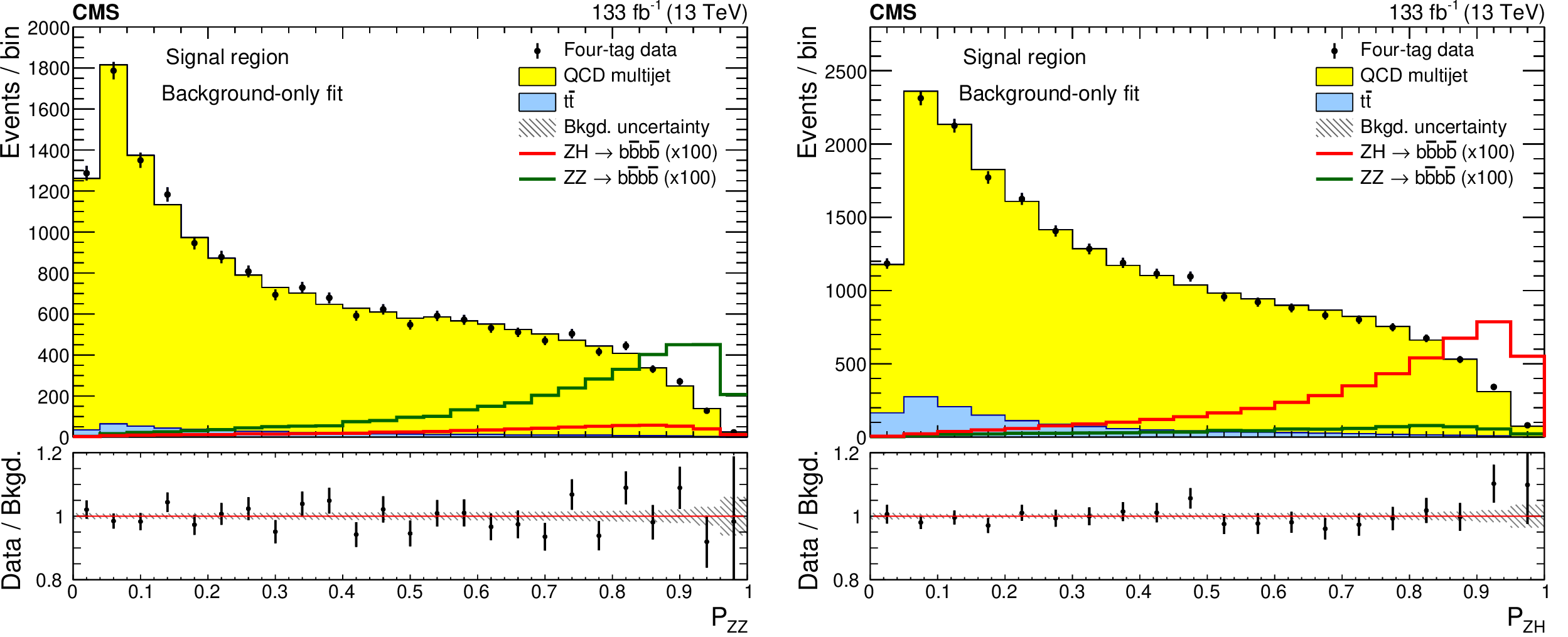
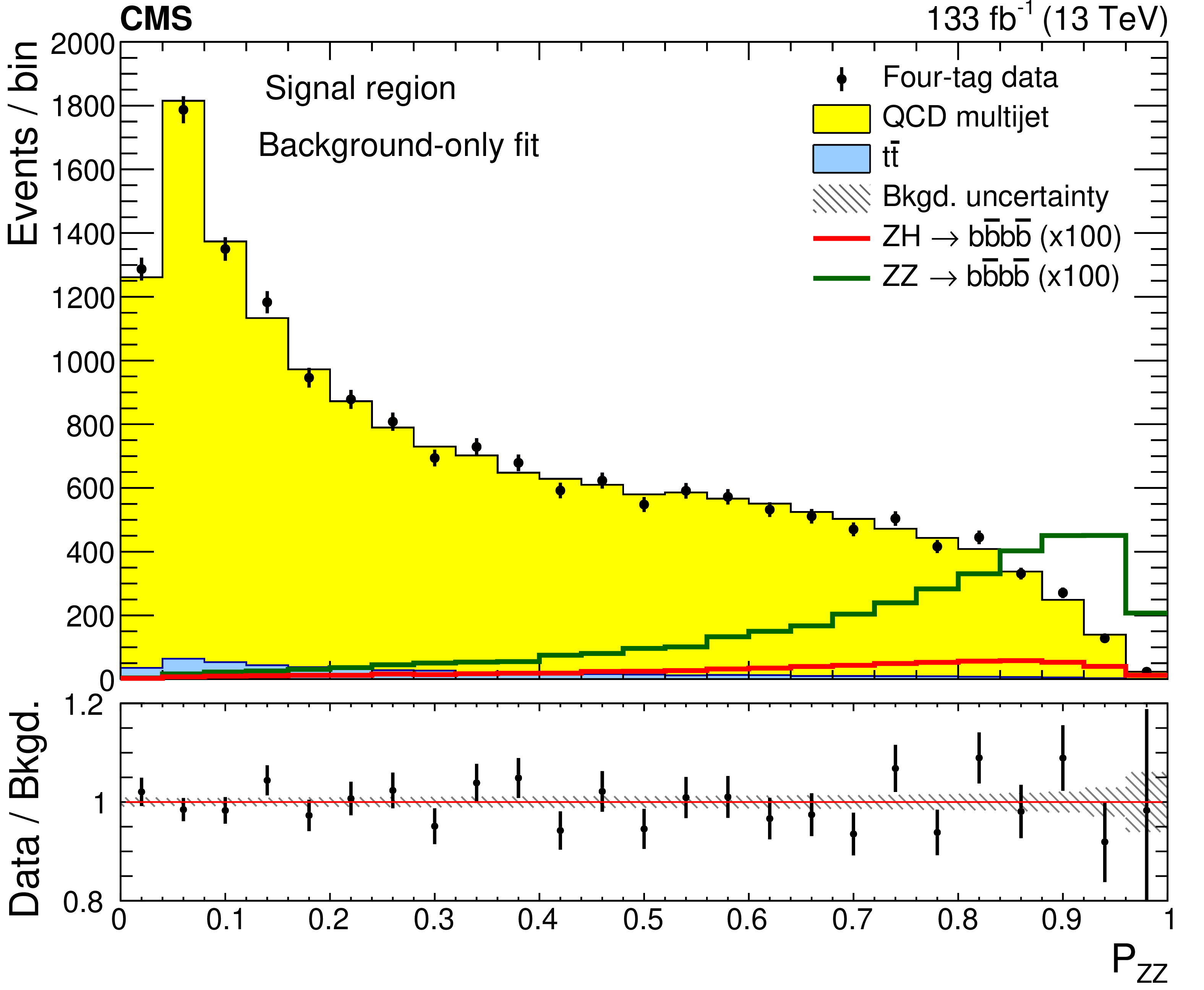
Additional Figure 10:
Distributions of signal probabilities for ZZ (left) and ZH (right) channels (points), along with the post background-only fit QCD multijet (yellow region) plus $ \mathrm{t} \bar{\mathrm{t}} $ (blue region) distributions. The expected ZH (red lines) and ZZ (blue lines) signal channel distributions are shown, multiplied by 100 for visibility. The lower panels display the ratio of the data to the total background, with the hatched area showing the uncertainty in the background. |
png pdf |
Additional Figure 10-a:
Distributions of signal probabilities for ZZ (left) and ZH (right) channels (points), along with the post background-only fit QCD multijet (yellow region) plus $ \mathrm{t} \bar{\mathrm{t}} $ (blue region) distributions. The expected ZH (red lines) and ZZ (blue lines) signal channel distributions are shown, multiplied by 100 for visibility. The lower panels display the ratio of the data to the total background, with the hatched area showing the uncertainty in the background. |

png pdf |
Additional Figure 10-b:
Distributions of signal probabilities for ZZ (left) and ZH (right) channels (points), along with the post background-only fit QCD multijet (yellow region) plus $ \mathrm{t} \bar{\mathrm{t}} $ (blue region) distributions. The expected ZH (red lines) and ZZ (blue lines) signal channel distributions are shown, multiplied by 100 for visibility. The lower panels display the ratio of the data to the total background, with the hatched area showing the uncertainty in the background. |

png pdf |
Additional Figure 11:
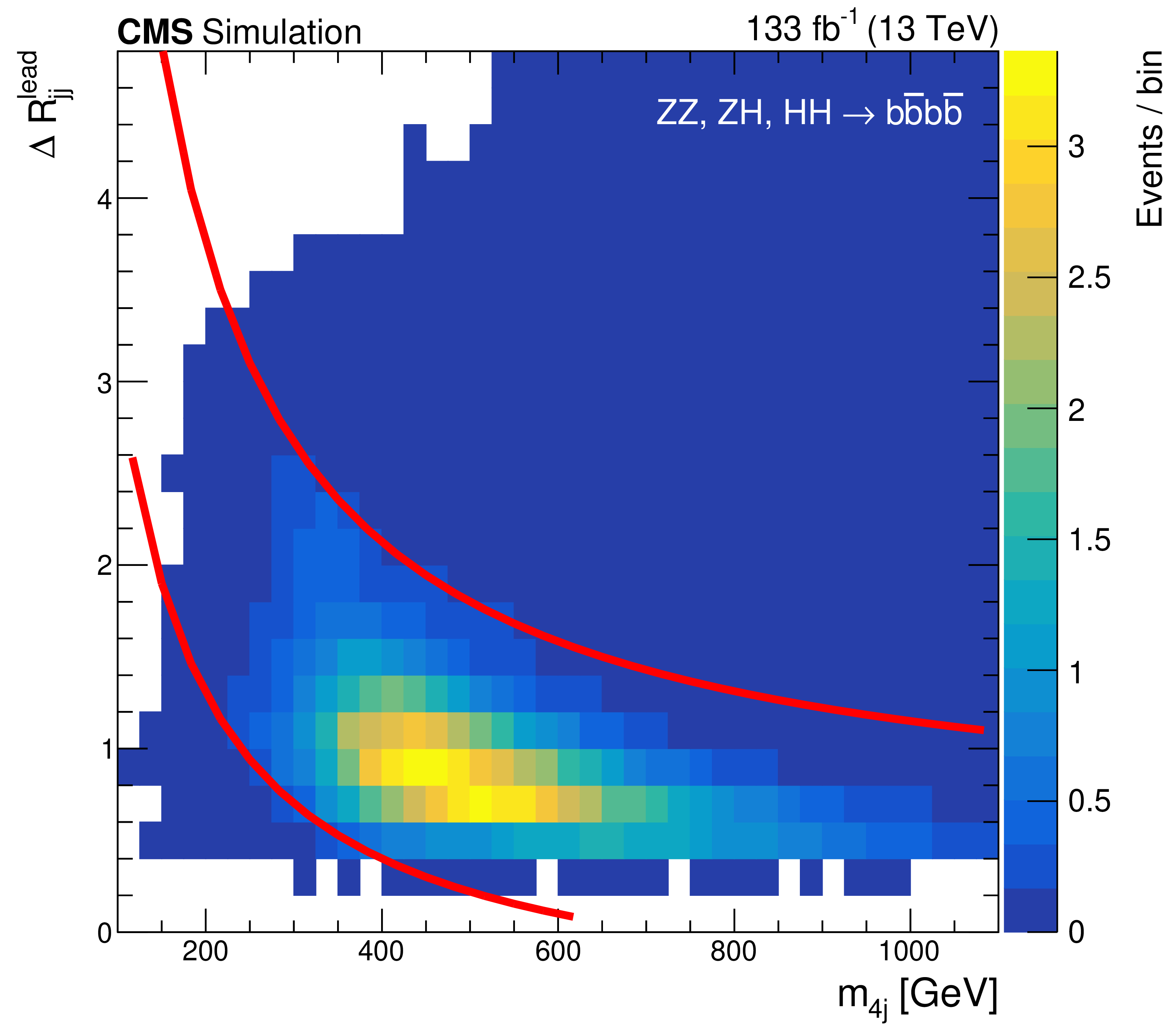
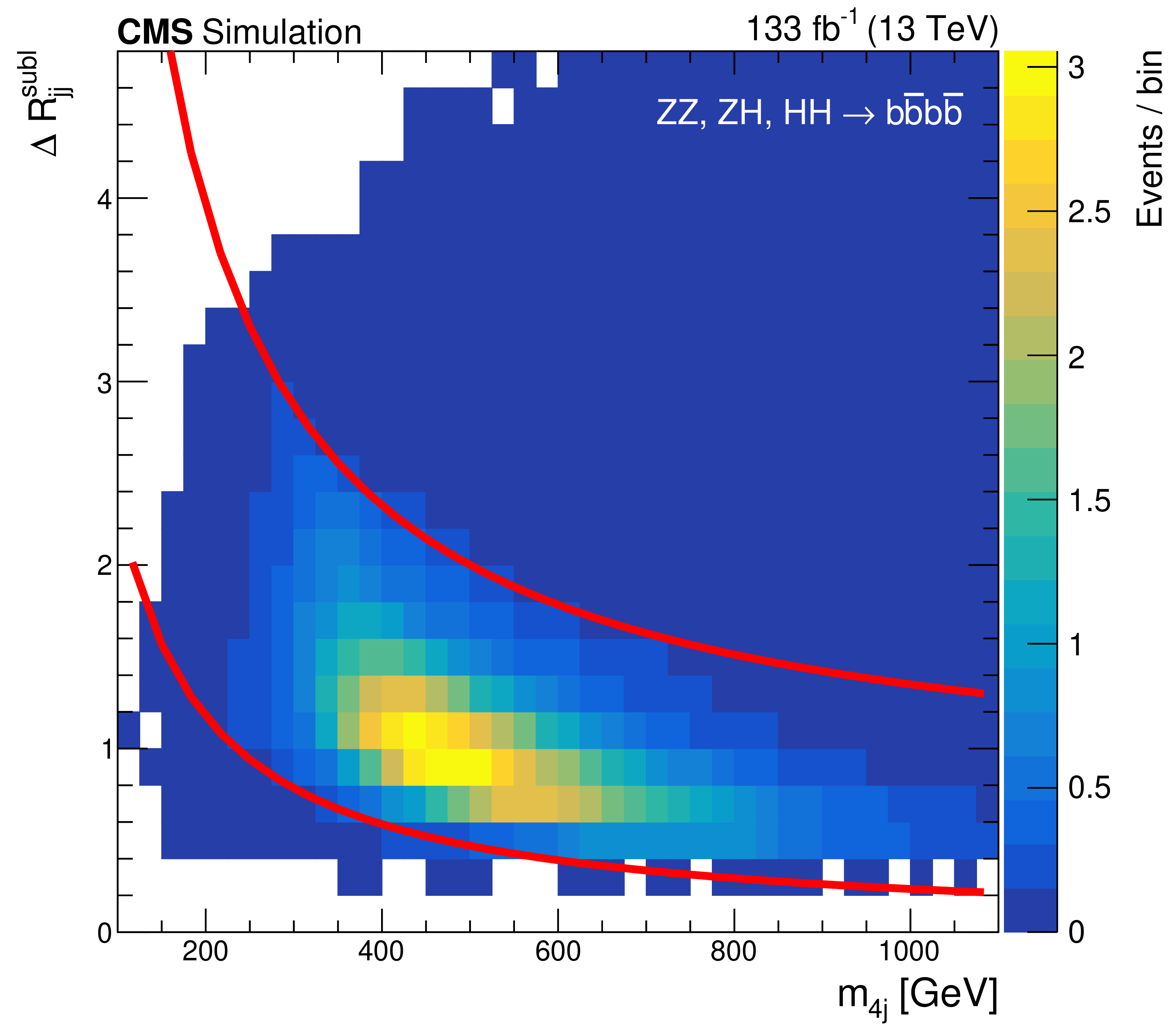
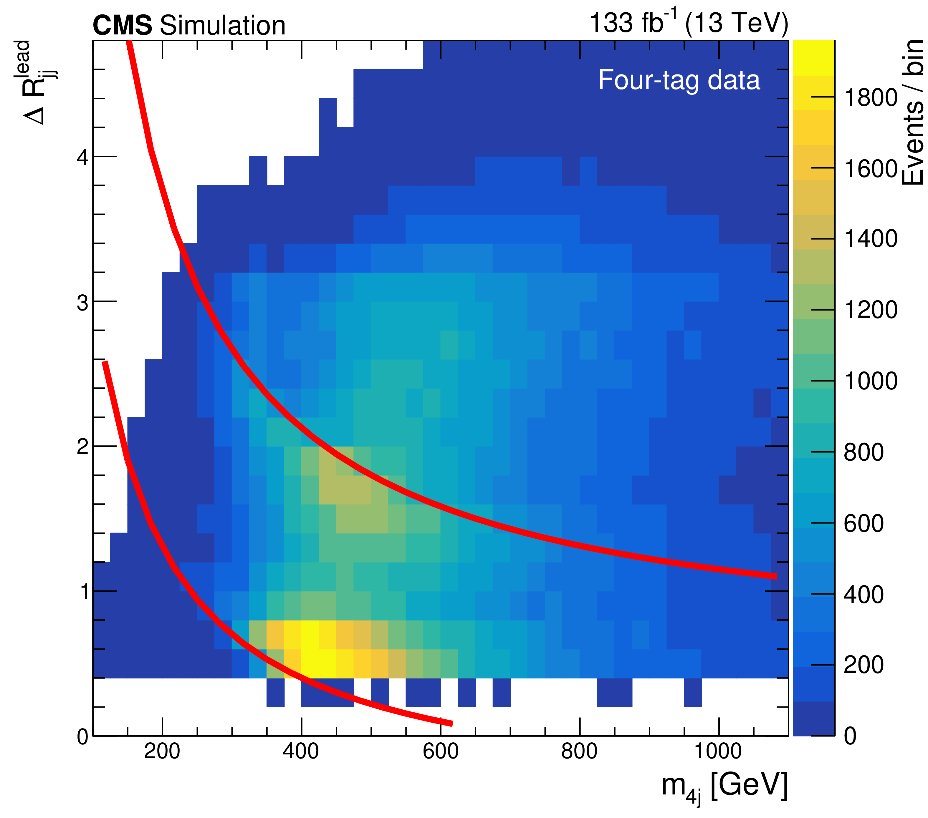
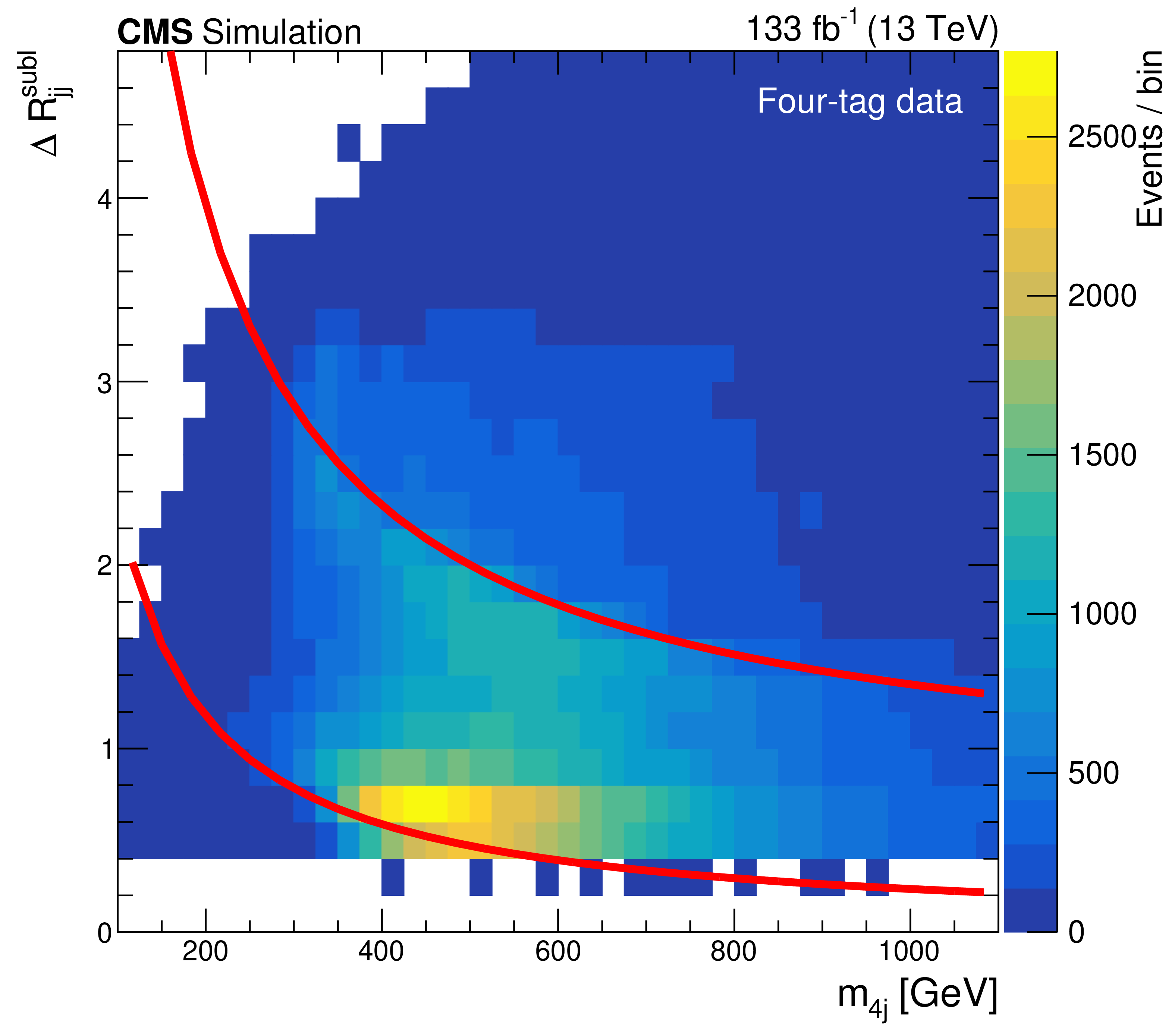
Distributions of $\Delta \text{R}_{\mathrm{jj}}^{\text{lead}}$ (left) and $\Delta \text{R}_{\mathrm{jj}}^{\text{subl}}$ (right) as a function of the four-jet mass for signal (top) and four-tag data (bottom). Events falling between the red lines satisfy the selection defined in Eq. 2. |
png pdf |
Additional Figure 11-a:
Distributions of $\Delta \text{R}_{\mathrm{jj}}^{\text{lead}}$ (left) and $\Delta \text{R}_{\mathrm{jj}}^{\text{subl}}$ (right) as a function of the four-jet mass for signal (top) and four-tag data (bottom). Events falling between the red lines satisfy the selection defined in Eq. 2. |
png pdf |
Additional Figure 11-b:
Distributions of $\Delta \text{R}_{\mathrm{jj}}^{\text{lead}}$ (left) and $\Delta \text{R}_{\mathrm{jj}}^{\text{subl}}$ (right) as a function of the four-jet mass for signal (top) and four-tag data (bottom). Events falling between the red lines satisfy the selection defined in Eq. 2. |
png pdf |
Additional Figure 11-c:
Distributions of $\Delta \text{R}_{\mathrm{jj}}^{\text{lead}}$ (left) and $\Delta \text{R}_{\mathrm{jj}}^{\text{subl}}$ (right) as a function of the four-jet mass for signal (top) and four-tag data (bottom). Events falling between the red lines satisfy the selection defined in Eq. 2. |
png pdf |
Additional Figure 11-d:
Distributions of $\Delta \text{R}_{\mathrm{jj}}^{\text{lead}}$ (left) and $\Delta \text{R}_{\mathrm{jj}}^{\text{subl}}$ (right) as a function of the four-jet mass for signal (top) and four-tag data (bottom). Events falling between the red lines satisfy the selection defined in Eq. 2. |
| References | ||||
| 1 | M. Cepeda et al. | Report from working group 2: Higgs physics at the HL-LHC and HE-LHC | CERN Yellow Rep. Monogr. 7 (2019) 221 | 1902.00134 |
| 2 | B. D. Micco, M. Gouzevitch, J. Mazzitelli, and C. Vernieri | Higgs boson potential at colliders: status and perspectives | Rev. Phys. 5 (2020) 100045 | 1910.00012 |
| 3 | CMS Collaboration | A portrait of the Higgs boson by the CMS experiment ten years after the discovery | Nature 607 (2022) 60 | CMS-HIG-22-001 2207.00043 |
| 4 | CMS Collaboration | Search for Higgs boson pair production in the four b quark final state in proton-proton collisions at $ \sqrt{s}= $ 13 TeV | PRL 129 (2022) 081802 | CMS-HIG-20-005 2202.09617 |
| 5 | ATLAS Collaboration | Search for Higgs boson pair production in the two bottom quarks plus two photons final state in pp collisions at $ \sqrt{s}= $ 13 TeV with the ATLAS detector | PRD 106 (2022) 052001 | 2112.11876 |
| 6 | CMS Collaboration | Search for nonresonant Higgs boson pair production in final state with two bottom quarks and two tau leptons in proton-proton collisions at $ \sqrt{s} = $ 13 TeV | PLB 842 (2023) 137531 | CMS-HIG-20-010 2206.09401 |
| 7 | ATLAS Collaboration | Search for resonant and non-resonant Higgs boson pair production in the $ \mathrm{b}\overline{\mathrm{b}}{\tau}^{+}{\tau}^{-} $ decay channel using 13 TeV pp collision data from the ATLAS detector | JHEP 07 (2023) 040 | 2209.10910 |
| 8 | CMS Collaboration | Search for nonresonant Higgs boson pair production in final states with two bottom quarks and two photons in proton-proton collisions at $ \sqrt{s} = $ 13 TeV | JHEP 03 (2021) 257 | CMS-HIG-19-018 2011.12373 |
| 9 | ATLAS Collaboration | Search for nonresonant pair production of Higgs bosons in the $ \mathrm{b}\overline{\mathrm{b}}\mathrm{b}\overline{\mathrm{b}} $ final state in pp collisions at $ \sqrt{s}= $ 13 TeV with the ATLAS detector | PRD 108 (2023) 052003 | 2301.03212 |
| 10 | CMS Collaboration | Search for nonresonant pair production of highly energetic Higgs bosons decaying to bottom quarks | PRL 131 (2023) 041803 | 2205.06667 |
| 11 | ATLAS Collaboration | Search for pair production of Higgs bosons in the $ \mathrm{b}\overline{\mathrm{b}}\mathrm{b}\overline{\mathrm{b}} $ final state using proton-proton collisions at $ \sqrt{s} = $ 13 TeV with the ATLAS detector | JHEP 01 (2019) 030 | 1804.06174 |
| 12 | CMS Collaboration | Search for resonant pair production of Higgs bosons decaying to bottom quark-antiquark pairs in proton-proton collisions at 13 TeV | JHEP 08 (2018) 152 | CMS-HIG-17-009 1806.03548 |
| 13 | ATLAS Collaboration | Search for pair production of Higgs bosons in the $ \mathrm{b}\overline{\mathrm{b}}\mathrm{b}\overline{\mathrm{b}} $ final state using proton--proton collisions at $ \sqrt{s} = $ 13 TeV with the ATLAS detector | PRD 94 (2016) 052002 | 1606.04782 |
| 14 | ATLAS Collaboration | Search for Higgs boson pair production in the $ \mathrm{b}\overline{\mathrm{b}}\mathrm{b}\overline{\mathrm{b}} $ final state from pp collisions at $ \sqrt{s} = $ 8 TeV with the ATLAS detector | EPJC 75 (2015) 412 | 1506.00285 |
| 15 | CMS Collaboration | Search for resonant pair production of Higgs bosons decaying to two bottom quark-antiquark pairs in proton-proton collisions at 8 TeV | PLB 749 (2015) 560 | CMS-HIG-14-013 1503.04114 |
| 16 | E. D. L. Cren | A note on the history of mark-recapture population estimates | Journal of Animal Ecology 34 (1965) 453 | |
| 17 | CDF Collaboration | Measurement of $ \sigma B(\textrm{W}\rightarrow\textrm{e}\nu) $ and $ \sigma B({\textrm{Z}}^{0}\rightarrow{\textrm{e}}^{+}{\textrm{e}}^{-}) $ in $ \overline{\rm{p}}\rm{p} $ collisions at $ \sqrt{s}= $ 1800 GeV | PRD 44 (1991) 29 | |
| 18 | O. Behnke, K. Kröninger, G. Schott, and T. Schörner-Sadenius | Data analysis in high energy physics: a practical guide to statistical methods | Wiley-VCH, Weinheim, 2013 link |
|
| 19 | P. De Castro Manzano et al. | Hemisphere mixing: a fully data-driven model of QCD multijet backgrounds for LHC searches | PoS EPS-HEP 370, 2017 link |
1712.02538 |
| 20 | CMS Collaboration | Search for nonresonant Higgs boson pair production in the $ \mathrm{b}\mathrm{b}\mathrm{b}\mathrm{b} $ final state at $ \sqrt{s} = $ 13 TeV | JHEP 04 (2019) 112 | CMS-HIG-17-017 1810.11854 |
| 21 | CMS Collaboration | Measurement of the ZZ production cross section and Z $ \to \ell^+\ell^-\ell'^+\ell'^- $ branching fraction in pp collisions at $ \sqrt{s} = $ 13 TeV | PLB 763 (2016) 280 | CMS-SMP-16-001 1607.08834 |
| 22 | LHC Higgs Cross Section Working Group | Handbook of LHC Higgs cross sections: 4. Deciphering the nature of the Higgs sector | CERN Report CERN-2017-002-M, 2016 link |
1610.07922 |
| 23 | CMS Collaboration | Measurements of $ {\mathrm{p}} {\mathrm{p}} \rightarrow {\mathrm{Z}} {\mathrm{Z}} $ production cross sections and constraints on anomalous triple gauge couplings at $ \sqrt{s} = 13\,\text {TeV} $ | EPJC 81 (2021) 200 | CMS-SMP-19-001 2009.01186 |
| 24 | ATLAS Collaboration | $ \rm{ZZ} \to \ell^{+}\ell^{-}\ell^{\prime +}\ell^{\prime -} $ cross-section measurements and search for anomalous triple gauge couplings in 13 TeV pp collisions with the ATLAS detector | PRD 97 (2018) 032005 | 1709.07703 |
| 25 | CMS Collaboration | Observation of Higgs boson decay to bottom quarks | PRL 121 (2018) 121801 | CMS-HIG-18-016 1808.08242 |
| 26 | ATLAS Collaboration | Observation of $ \rm{H} \rightarrow \mathrm{b}\overline{\mathrm{b}} $ decays and VH production with the ATLAS detector | PLB 786 (2018) 59 | 1808.08238 |
| 27 | CMS Collaboration | Measurement of simplified template cross sections of the Higgs boson produced in association with W or Z bosons in the H $ \to \mathrm{b}\overline{\mathrm{b}} $ decay channel in proton-proton collisions at $ \sqrt{s} $ = 13 TeV | Submitted to Physical Review D, 2023 | CMS-HIG-20-001 2312.07562 |
| 28 | CMS Collaboration | HEPData record for this analysis | link | |
| 29 | CMS Collaboration | The CMS experiment at the CERN LHC | JINST 3 (2008) S08004 | |
| 30 | CMS Collaboration | Development of the CMS detector for the CERN LHC Run 3 | CMS-PRF-21-001 2309.05466 |
|
| 31 | CMS Collaboration | Performance of the CMS Level-1 trigger in proton-proton collisions at $ \sqrt{s} = $ 13 TeV | JINST 15 (2020) P10017 | CMS-TRG-17-001 2006.10165 |
| 32 | CMS Collaboration | The CMS trigger system | JINST 12 (2017) P01020 | CMS-TRG-12-001 1609.02366 |
| 33 | CMS Collaboration | Electron and photon reconstruction and identification with the CMS experiment at the CERN LHC | JINST 16 (2021) P05014 | CMS-EGM-17-001 2012.06888 |
| 34 | CMS Collaboration | Performance of the CMS muon detector and muon reconstruction with proton-proton collisions at $ \sqrt{s}= $ 13 TeV | JINST 13 (2018) P06015 | CMS-MUO-16-001 1804.04528 |
| 35 | CMS Collaboration | Description and performance of track and primary-vertex reconstruction with the CMS tracker | JINST 9 (2014) P10009 | CMS-TRK-11-001 1405.6569 |
| 36 | CMS Collaboration | Particle-flow reconstruction and global event description with the CMS detector | JINST 12 (2017) P10003 | CMS-PRF-14-001 1706.04965 |
| 37 | CMS Collaboration | Technical proposal for the Phase-II upgrade of the Compact Muon Solenoid | CMS Technical Proposal CERN-LHCC-2015-010, CMS-TDR-15-02, CERN, 2015 CDS |
|
| 38 | M. Cacciari, G. P. Salam, and G. Soyez | The anti-$ k_{\mathrm{T}} $ jet clustering algorithm | JHEP 04 (2008) 063 | 0802.1189 |
| 39 | M. Cacciari, G. P. Salam, and G. Soyez | FastJet user manual | EPJC 72 (2012) 1896 | 1111.6097 |
| 40 | CMS Collaboration | Pileup mitigation at CMS in $ \sqrt{s}= $ 13 TeV data | JINST 15 (2020) P09018 | CMS-JME-18-001 2003.00503 |
| 41 | CMS Collaboration | Jet energy scale and resolution in the CMS experiment in proton-proton collisions at $ \sqrt{s}= $ 8 TeV | JINST 12 (2017) P02014 | CMS-JME-13-004 1607.03663 |
| 42 | CMS Collaboration | Jet energy scale and resolution measurement with Run-2 legacy data collected by CMS at $ \sqrt{s}= $ 13 TeV | CMS Detector Performance Summary CMS-DP-2021-033, CERN, 2021 CDS |
|
| 43 | E. Bols et al. | Jet flavour classification using DeepJet | JINST 15 (2020) P12012 | 2008.10519 |
| 44 | CMS Collaboration | Precision luminosity measurement in proton-proton collisions at $ \sqrt{s} = $ 13 TeV in 2015 and 2016 at CMS | EPJC 81 (2021) 800 | CMS-LUM-17-003 2104.01927 |
| 45 | CMS Collaboration | CMS luminosity measurement for the 2017 data-taking period at $ \sqrt{s} = $ 13 TeV | CMS Physics Analysis Summary , CERN, 2017 CMS-PAS-LUM-17-004 |
CMS-PAS-LUM-17-004 |
| 46 | CMS Collaboration | CMS luminosity measurement for the 2018 data-taking period at $ \sqrt{s} = $ 13 TeV | CMS Physics Analysis Summary , CERN, 2019 CMS-PAS-LUM-18-002 |
CMS-PAS-LUM-18-002 |
| 47 | CMS Collaboration | Identification of heavy-flavour jets with the CMS detector in pp collisions at 13 TeV | JINST 13 (2018) P05011 | CMS-BTV-16-002 1712.07158 |
| 48 | S. Frixione, P. Nason, and G. Ridolfi | A positive-weight next-to-leading-order Monte Carlo for heavy flavour hadroproduction | JHEP 09 (2007) 126 | 0707.3088 |
| 49 | S. Frixione, P. Nason, and C. Oleari | Matching NLO QCD computations with parton shower simulations: the POWHEG method | JHEP 11 (2007) 070 | 0709.2092 |
| 50 | J. M. Campbell, R. K. Ellis, P. Nason, and E. Re | Top-pair production and decay at NLO matched with parton showers | JHEP 04 (2015) 114 | 1412.1828 |
| 51 | J. Alwall et al. | The automated computation of tree-level and next-to-leading order differential cross sections, and their matching to parton shower simulations | JHEP 07 (2014) 79 | 1405.0301 |
| 52 | R. Frederix and S. Frixione | Merging meets matching in MC@NLO | JHEP 12 (2012) 061 | 1209.6215 |
| 53 | K. Mimasu, V. Sanz, and C. Williams | Higher order QCD predictions for associated Higgs production with anomalous couplings to gauge bosons | JHEP 08 (2016) 039 | 1512.02572 |
| 54 | K. Hamilton, P. Nason, and G. Zanderighi | MINLO: Multi-scale improved NLO | JHEP 10 (2012) 155 | 1206.3572 |
| 55 | G. Luisoni, P. Nason, C. Oleari, and F. Tramontano | HW/HZ + 0 and 1 jet at NLO with the POWHEG BOX interfaced to GoSam and their merging within MiNLO | JHEP 10 (2013) 083 | 1306.2542 |
| 56 | A. Djouadi, J. Kalinowski, M. Mühlleitner, and M. Spira | Hdecay: Twenty++ years after | Computer Physics Communications 238 (2019) | |
| 57 | Particle Data Group , R. L. Workman et al. | Review of particle physics | Prog. Theor. Exp. Phys. 2022 (2022) 083C01 | |
| 58 | G. Heinrich et al. | NLO predictions for Higgs boson pair production with full top quark mass dependence matched to parton showers | JHEP 08 (2017) 088 | 1703.09252 |
| 59 | S. Dawson, S. Dittmaier, and M. Spira | Neutral Higgs boson pair production at hadron colliders: QCD corrections | PRD 58 (1998) 115012 | hep-ph/9805244 |
| 60 | S. Borowka et al. | Higgs boson pair production in gluon fusion at next-to-leading order with full top-quark mass dependence | PRL 117 (2016) 012001 | 1604.06447 |
| 61 | J. Baglio et al. | Gluon fusion into Higgs pairs at NLO QCD and the top mass scheme | EPJC 79 (2019) 459 | 1811.05692 |
| 62 | D. de Florian and J. Mazzitelli | Higgs boson pair production at next-to-next-to-leading order in QCD | PRL 111 (2013) 201801 | 1309.6594 |
| 63 | D. Y. Shao, C. S. Li, H. T. Li, and J. Wang | Threshold resummation effects in Higgs boson pair production at the LHC | JHEP 07 (2013) 169 | 1301.1245 |
| 64 | D. de Florian and J. Mazzitelli | Higgs pair production at next-to-next-to-leading logarithmic accuracy at the LHC | JHEP 09 (2015) 053 | 1505.07122 |
| 65 | M. Grazzini et al. | Higgs boson pair production at NNLO with top quark mass effects | JHEP 05 (2018) 059 | 1803.02463 |
| 66 | J. Baglio et al. | $ \mathrm{g}\mathrm{g}\to \mathrm{H}\mathrm{H} $: Combined uncertainties | PRD 103 (2021) 056002 | 2008.11626 |
| 67 | T. Sjöstrand et al. | An introduction to PYTHIA 8.2 | Comp. Phys. Commun. 191 (2015) 159 | 1410.3012 |
| 68 | CMS Collaboration | Extraction and validation of a new set of CMS PYTHIA8 tunes from underlying-event measurements | EPJC 80 (2020) 4 | CMS-GEN-17-001 1903.12179 |
| 69 | CMS Collaboration | Event generator tunes obtained from underlying event and multiparton scattering measurements | EPJC 76 (2016) 155 | CMS-GEN-14-001 1512.00815 |
| 70 | NNPDF Collaboration | Parton distributions for the LHC Run II | JHEP 04 (2015) 040 | 1410.8849 |
| 71 | R. D. Ball et al. | Parton distributions from high-precision collider data | EPJC 77 (2017) 663 | 1706.00428 |
| 72 | GEANT4 Collaboration | GEANT4---a simulation toolkit | NIM A 506 (2003) 250 | |
| 73 | CMS Collaboration | Evidence for the Higgs boson decay to a bottom quark-antiquark pair | PLB 780 (2018) 501 | CMS-HIG-16-044 1709.07497 |
| 74 | W. Shang, K. Sohn, D. Almeida, and H. Lee | Understanding and improving convolutional neural networks via concatenated rectified linear units | in Proc. 33rd Int. Conf. on Machine Learning, volume 48, PMLR, 2016 link |
1603.05201 |
| 75 | K. He, X. Zhang, S. Ren, and J. Sun | Deep residual learning for image recognition | in IEEE Conf, in Computer Vision and Pattern Recognition (CVPR), 2016 link |
1512.03385 |
| 76 | A. Vaswani et al. | Attention is all you need | in Advances in Neural Information Processing Systems, volume 30. Curran Associates, Inc, 2017 link |
1706.03762 |
| 77 | R. A. Fisher | On the interpretation of $ \chi^2 $ from contingency tables, and the calculation of $ p $ | J. Royal Stat. Soc. (1922) | |
| 78 | T. Junk | Confidence level computation for combining searches with small statistics | NIM A 434 (1999) 435 | hep-ex/9902006 |
| 79 | A. L. Read | Presentation of search results: The CL$ _{\text{s}} $ technique | JPG 28 (2002) 2693 | |
|
|
Compact Muon Solenoid LHC, CERN |
|

|

|

|

|

|