

Compact Muon Solenoid
LHC, CERN
| CMS-TOP-17-015 ; CERN-EP-2018-177 | ||
| Study of the underlying event in top quark pair production in pp collisions at 13 TeV | ||
| CMS Collaboration | ||
| 8 July 2018 | ||
| Eur. Phys. J. C 79 (2019) 123 | ||
| Abstract: Measurements of normalized differential cross sections as functions of the multiplicity and kinematic variables of charged-particle tracks from the underlying event in top quark and antiquark pair production are presented. The measurements are performed in proton-proton collisions at a center-of-mass energy of 13 TeV, and are based on data collected by the CMS experiment at the LHC in 2016 corresponding to an integrated luminosity of 35.9 fb$^{-1}$. Events containing one electron, one muon, and two jets from the hadronization and fragmentation of b quarks are used. These measurements characterize, for the first time, properties of the underlying event in top quark pair production and show no deviation from the universality hypothesis at energy scales typically above twice the top quark mass. | ||
| Links: e-print arXiv:1807.02810 [hep-ex] (PDF) ; CDS record ; inSPIRE record ; CADI line (restricted) ; | ||
| Figures | |
png pdf |
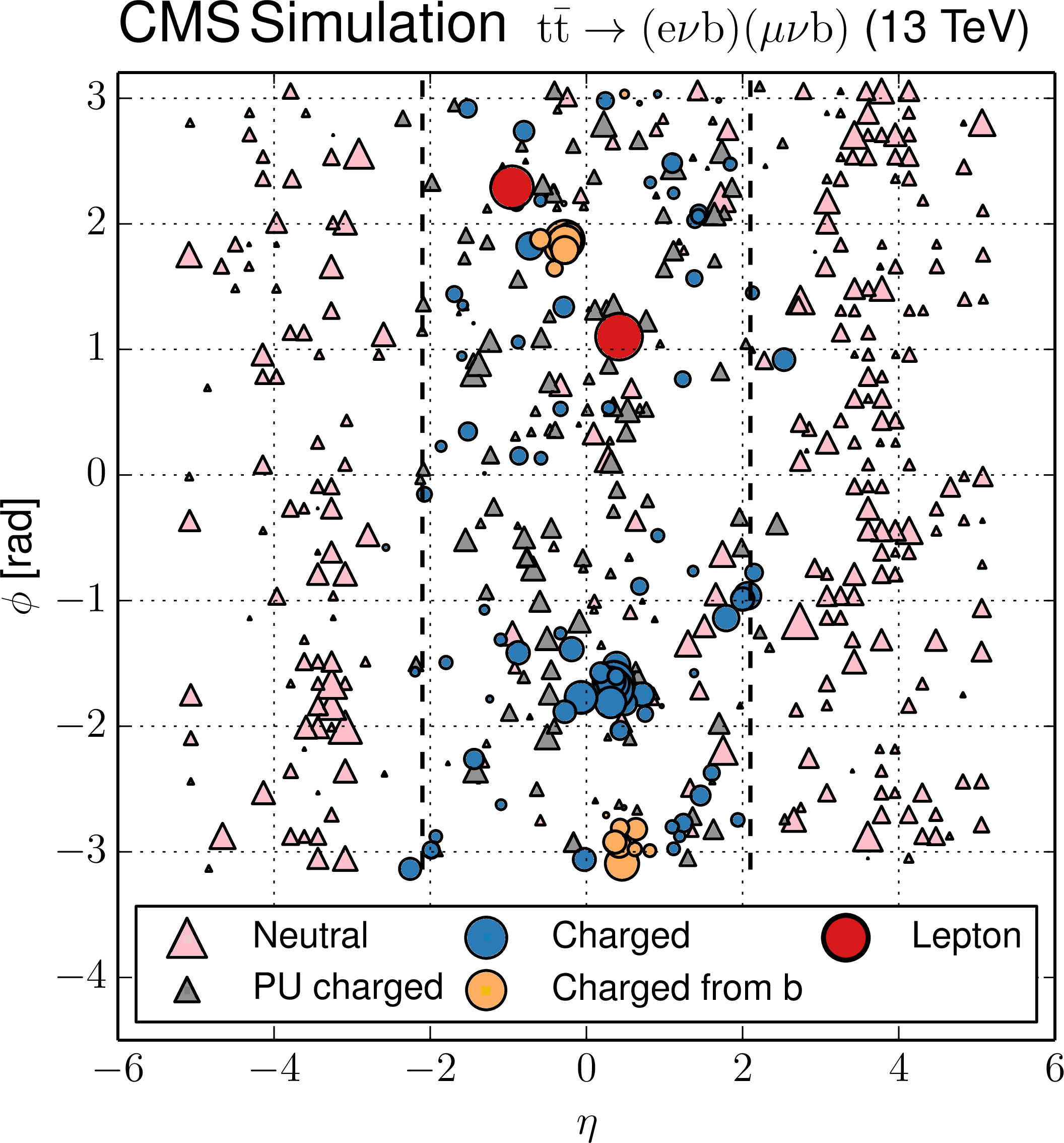
Figure 1:
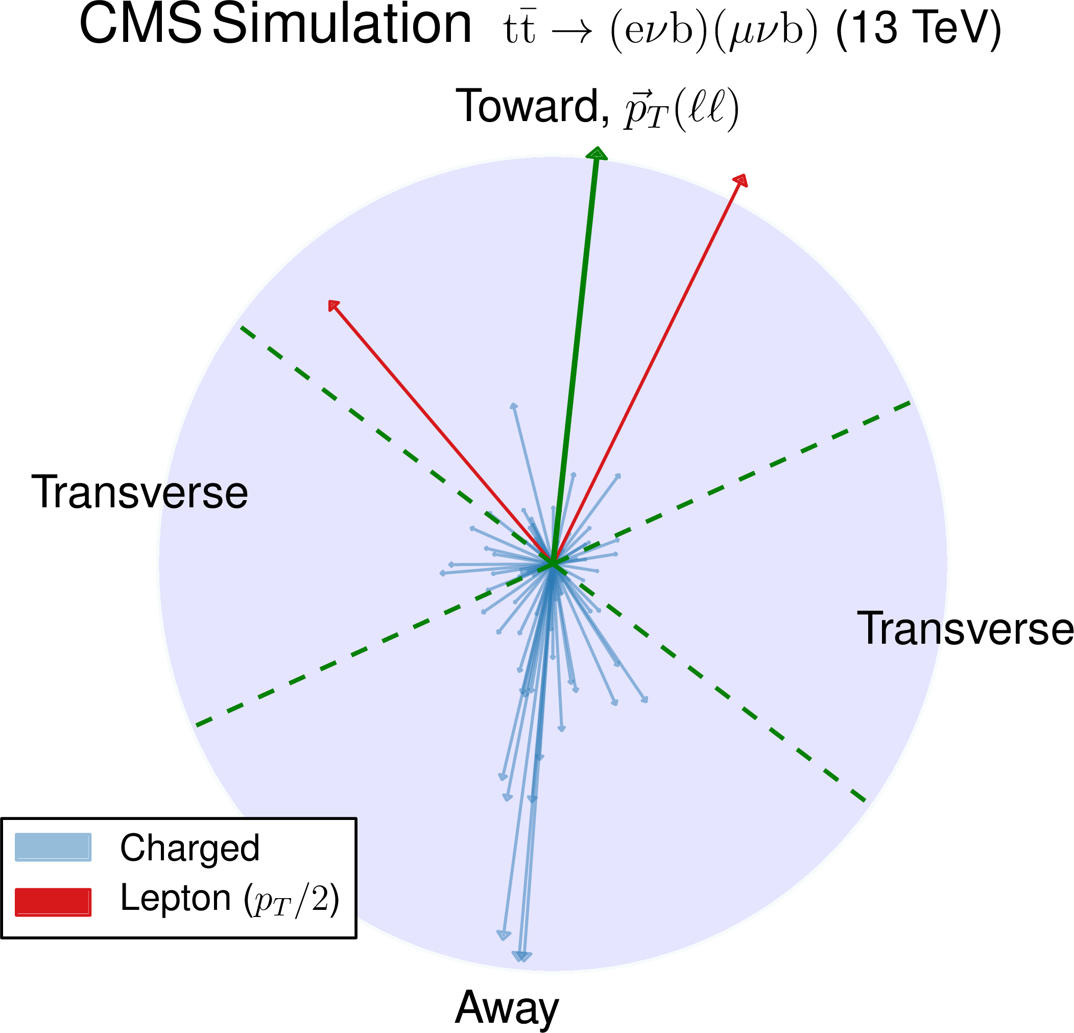
Distribution of all PF candidates reconstructed in a POWHEG+PYTHIA8 simulated ${{\mathrm {t}\overline {\mathrm {t}}}}$ event in the $\eta $-$\phi $ plane. Only particles with $ {p_{\mathrm {T}}} > $ 900 MeV are shown, with a marker whose are is proportional to the particle $ {p_{\mathrm {T}}} $. The fiducial region in $\eta $ is represented by the dashed lines. |
png pdf |
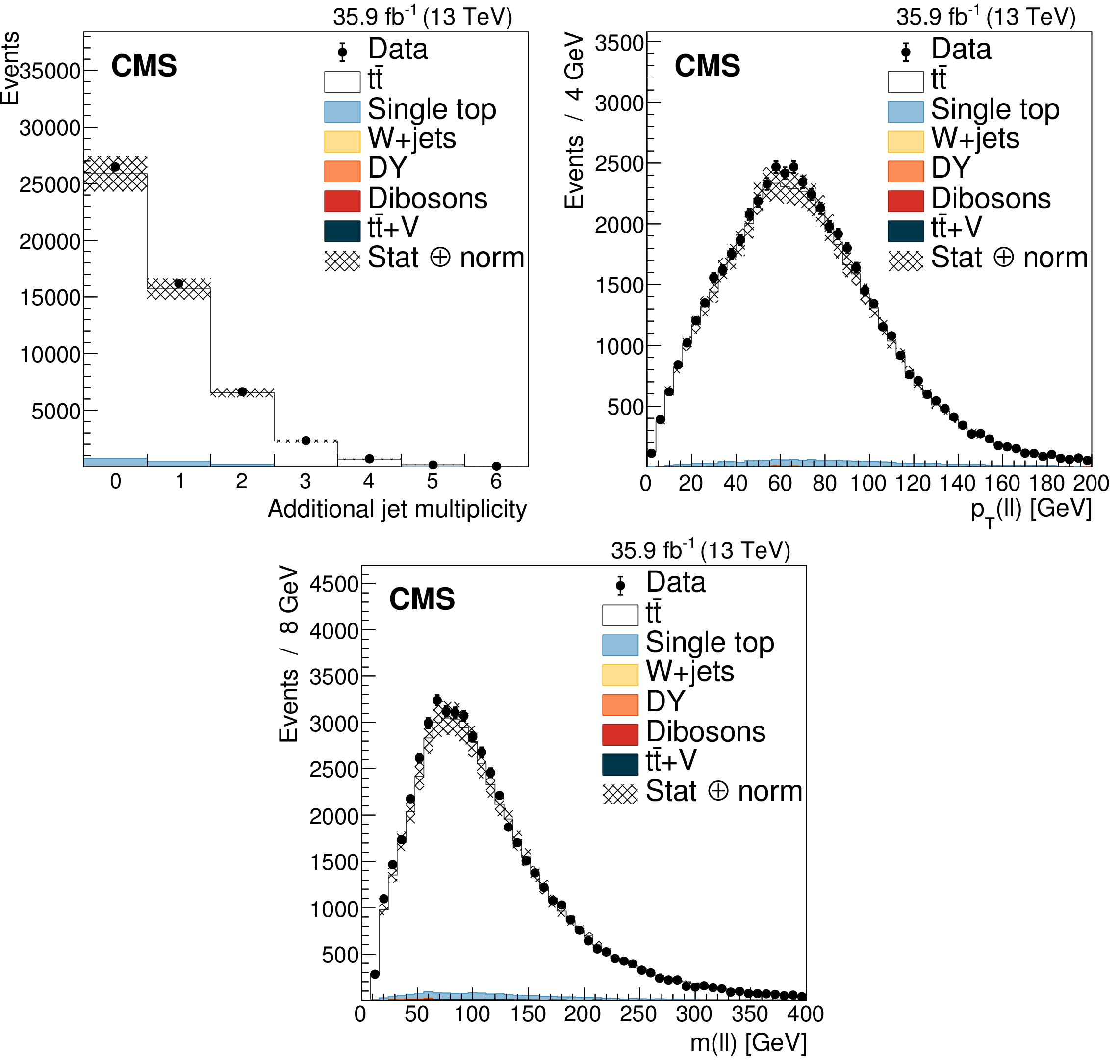
Figure 2:
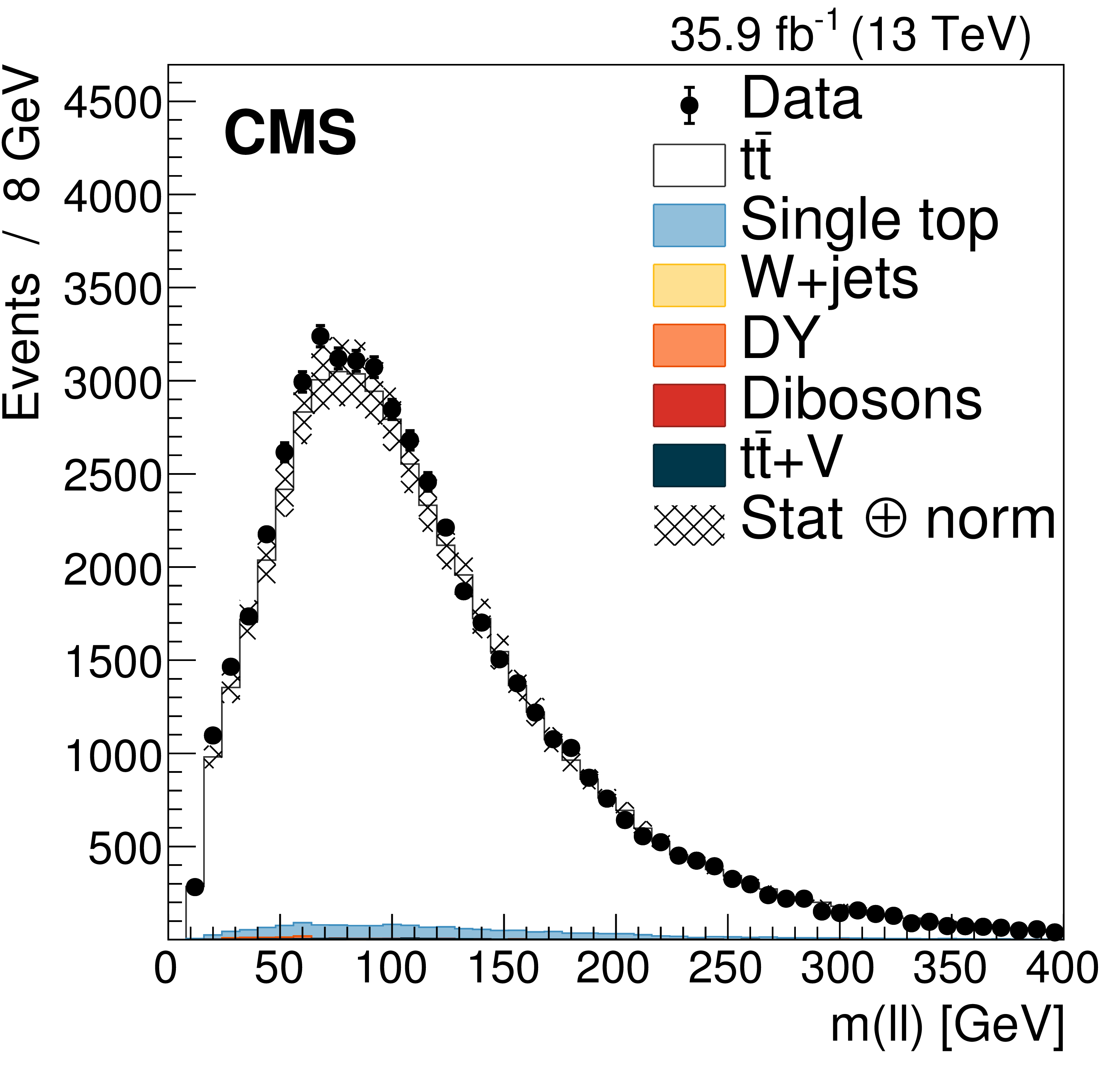
Distributions of the variables used to categorize the study of the UE. Upper left: multiplicity of additional jets ($ {p_{\mathrm {T}}} > $ 30 GeV). Upper right: $ {{p_{\mathrm {T}}} (\ell \ell)} $. Lower: $ {m(\ell \ell)} $. The distributions in data are compared to the sum of the expectations for the signal and backgrounds. The shaded band represents the uncertainty associated to the integrated luminosity and the theoretical value of the ${{\mathrm {t}\overline {\mathrm {t}}}}$ cross section. |
png pdf |
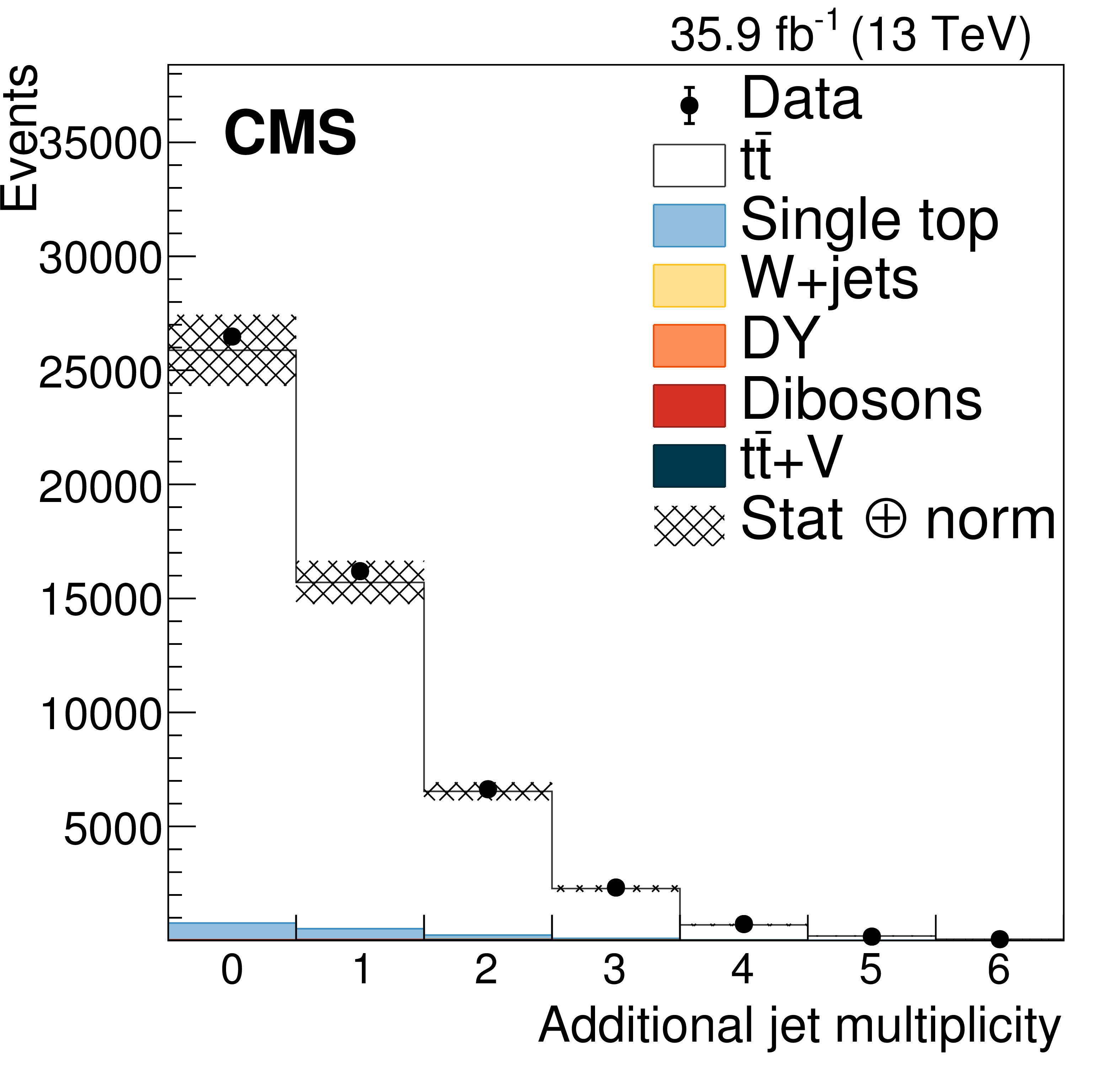
Figure 2-a:
Distribution of the multiplicity of additional jets ($ {p_{\mathrm {T}}} > $ 30 GeV). The distribution in data is compared to the sum of the expectations for the signal and backgrounds. The shaded band represents the uncertainty associated to the integrated luminosity and the theoretical value of the ${{\mathrm {t}\overline {\mathrm {t}}}}$ cross section. |
png pdf |
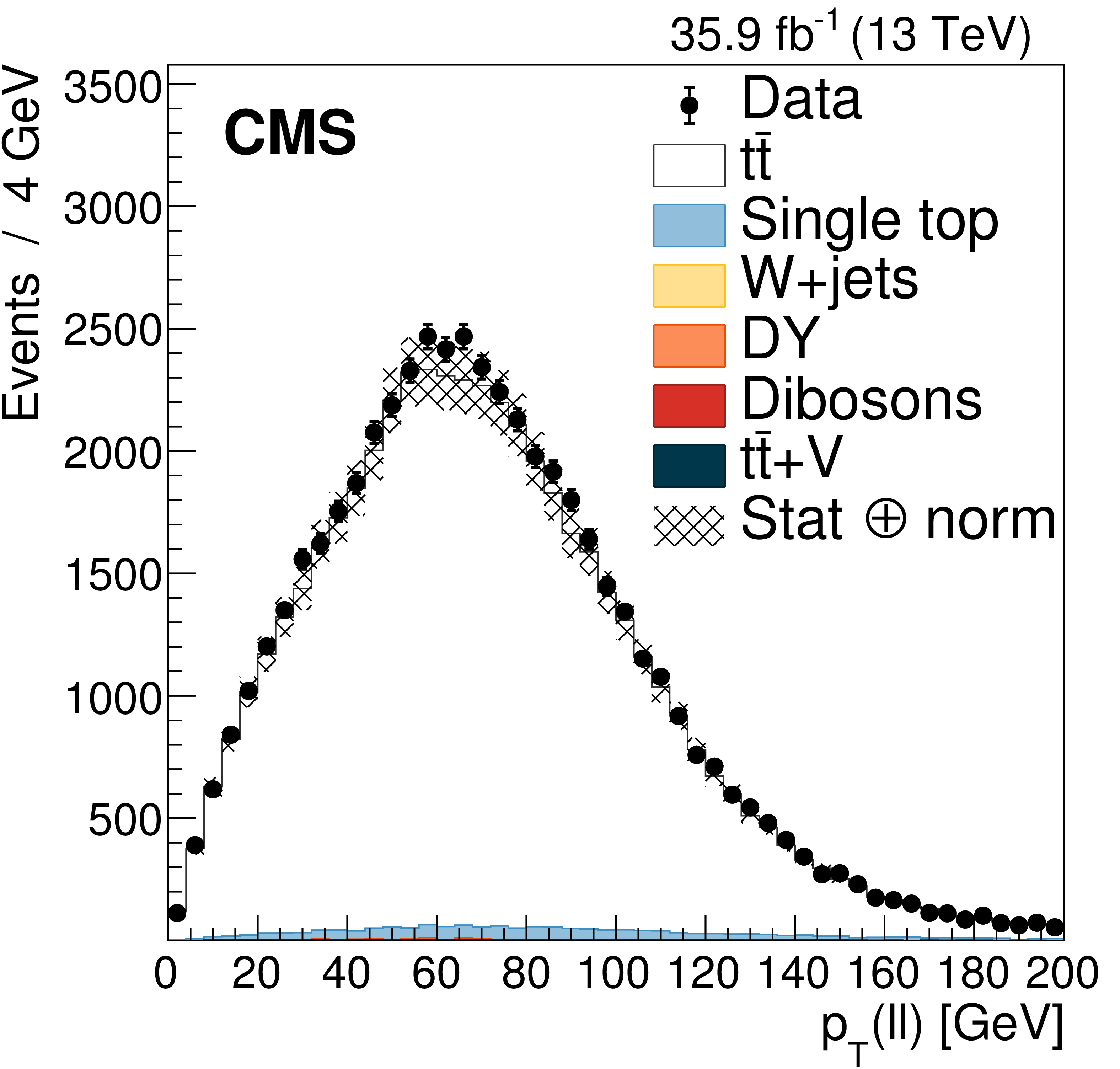
Figure 2-b:
Distribution of $ {{p_{\mathrm {T}}} (\ell \ell)} $. The distribution in data is compared to the sum of the expectations for the signal and backgrounds. The shaded band represents the uncertainty associated to the integrated luminosity and the theoretical value of the ${{\mathrm {t}\overline {\mathrm {t}}}}$ cross section. |
png pdf |
Figure 2-c:
Distribution of $ {m(\ell \ell)} $. The distribution in data is compared to the sum of the expectations for the signal and backgrounds. The shaded band represents the uncertainty associated to the integrated luminosity and the theoretical value of the ${{\mathrm {t}\overline {\mathrm {t}}}}$ cross section. |
png pdf |
Figure 3:
Display of the transverse momentum of the selected charged particles, the two leptons, and the dilepton pair in the transverse plane corresponding to the same event as in Fig. 1. The $ {p_{\mathrm {T}}} $ of the particles is proportional to the length of the arrows and the dashed lines represent the regions that are defined relative to the $ {{\vec{p}_{\mathrm {T}}} (\ell \ell)} $ direction. For clarity, the $ {p_{\mathrm {T}}} $ of the leptons has been rescaled by a factor of 0.5. |
png pdf |
Figure 4:
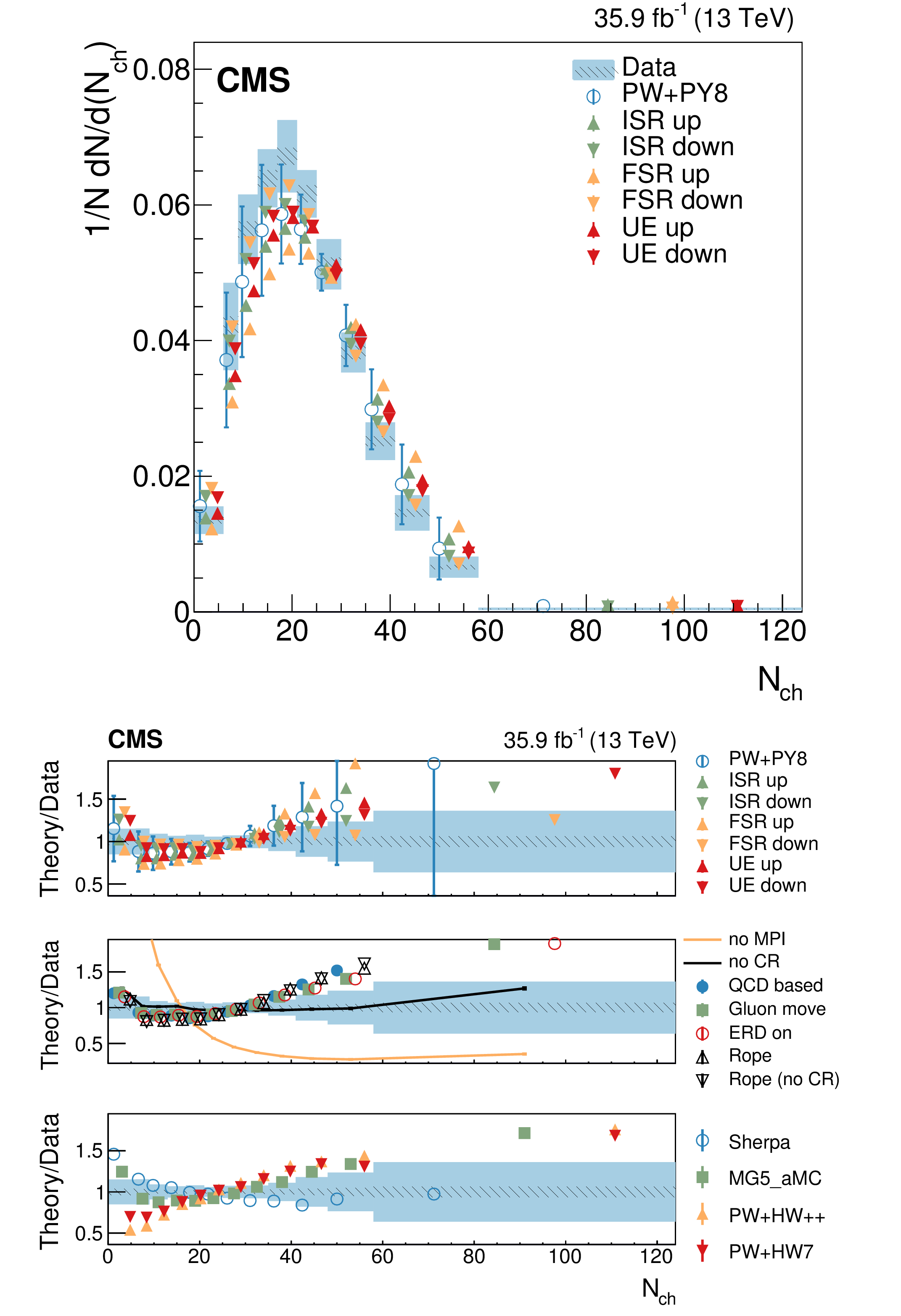
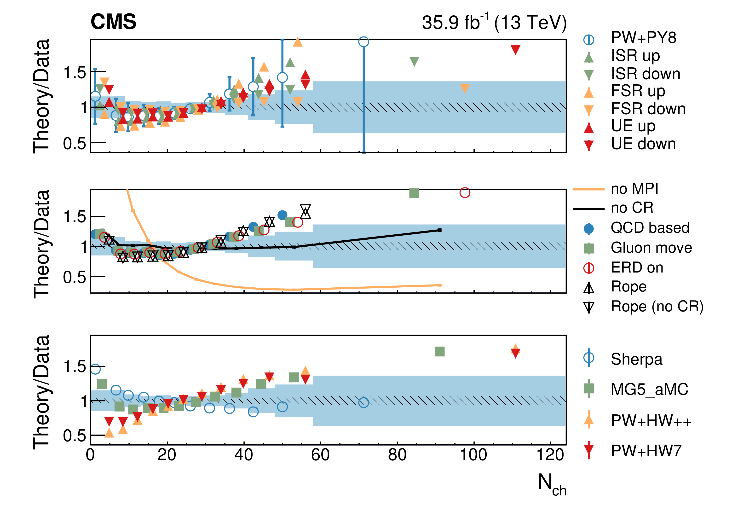
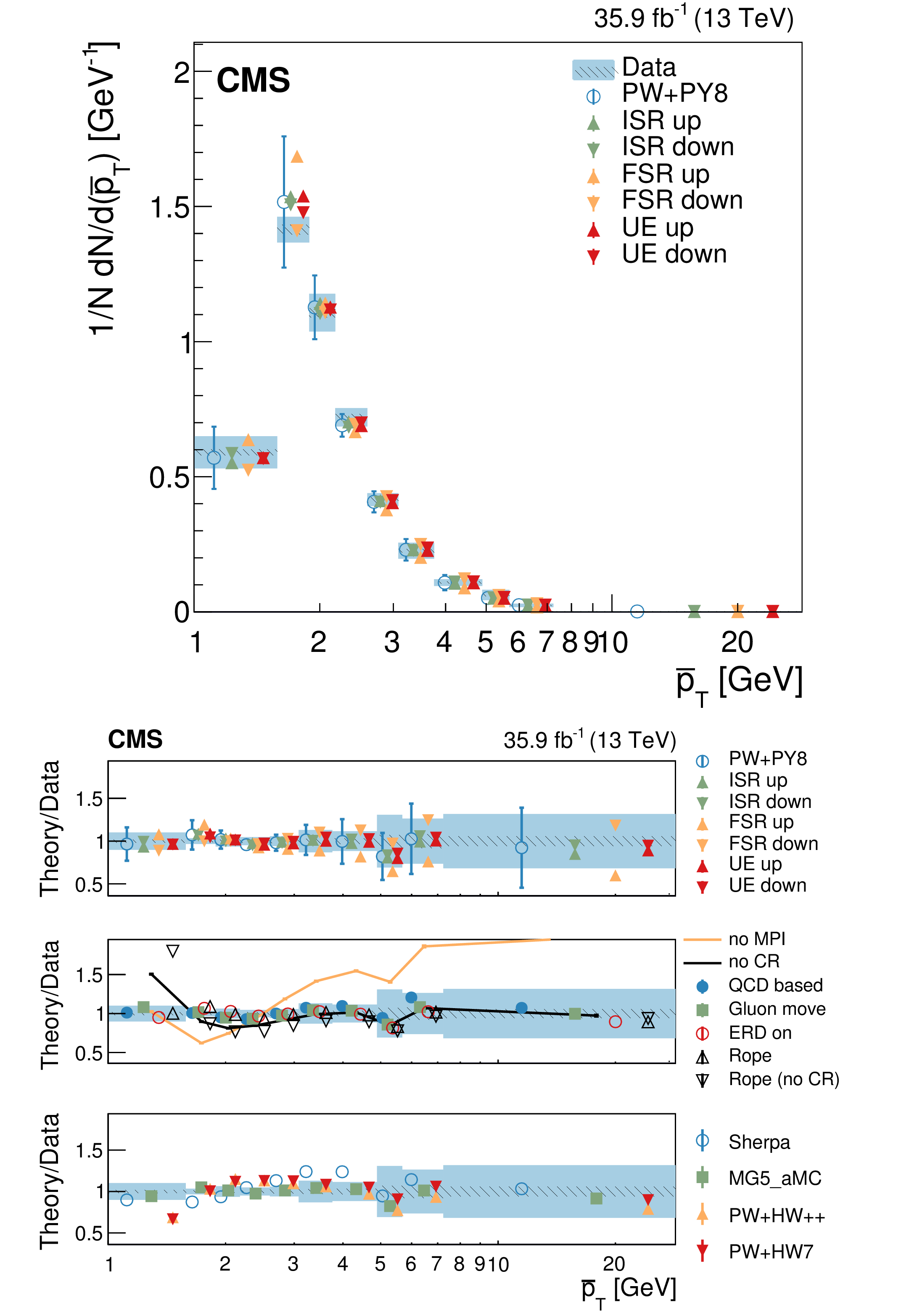
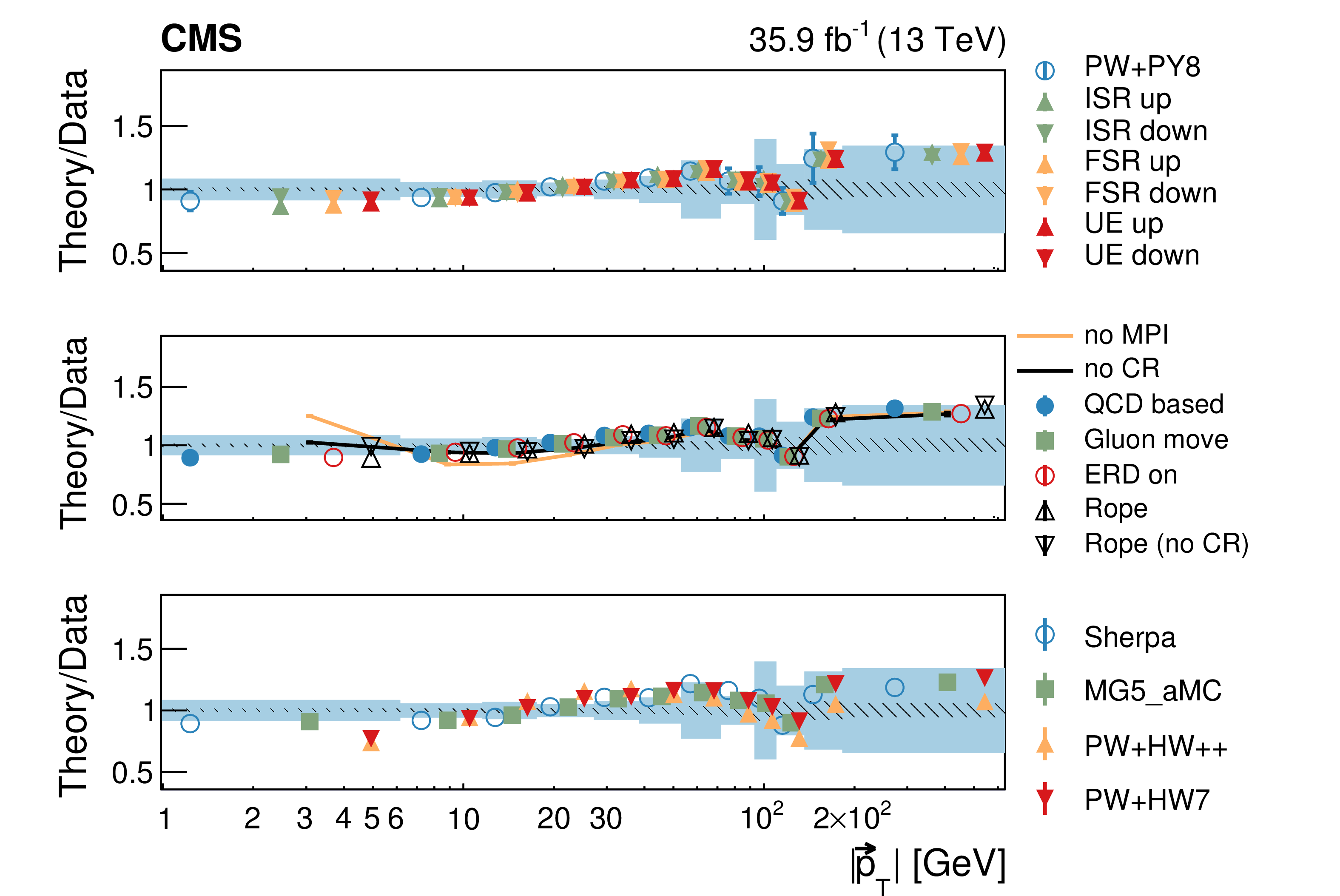
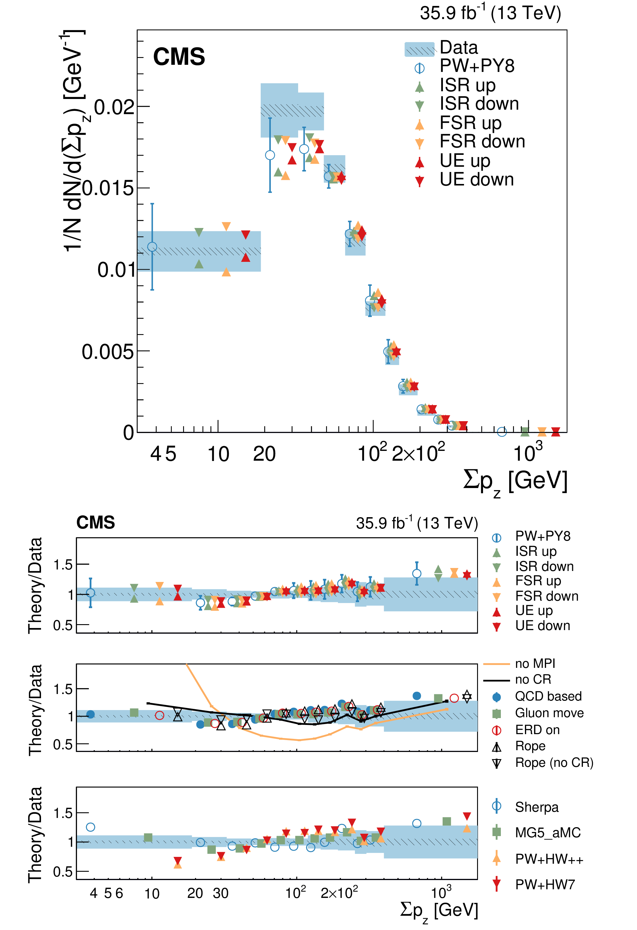
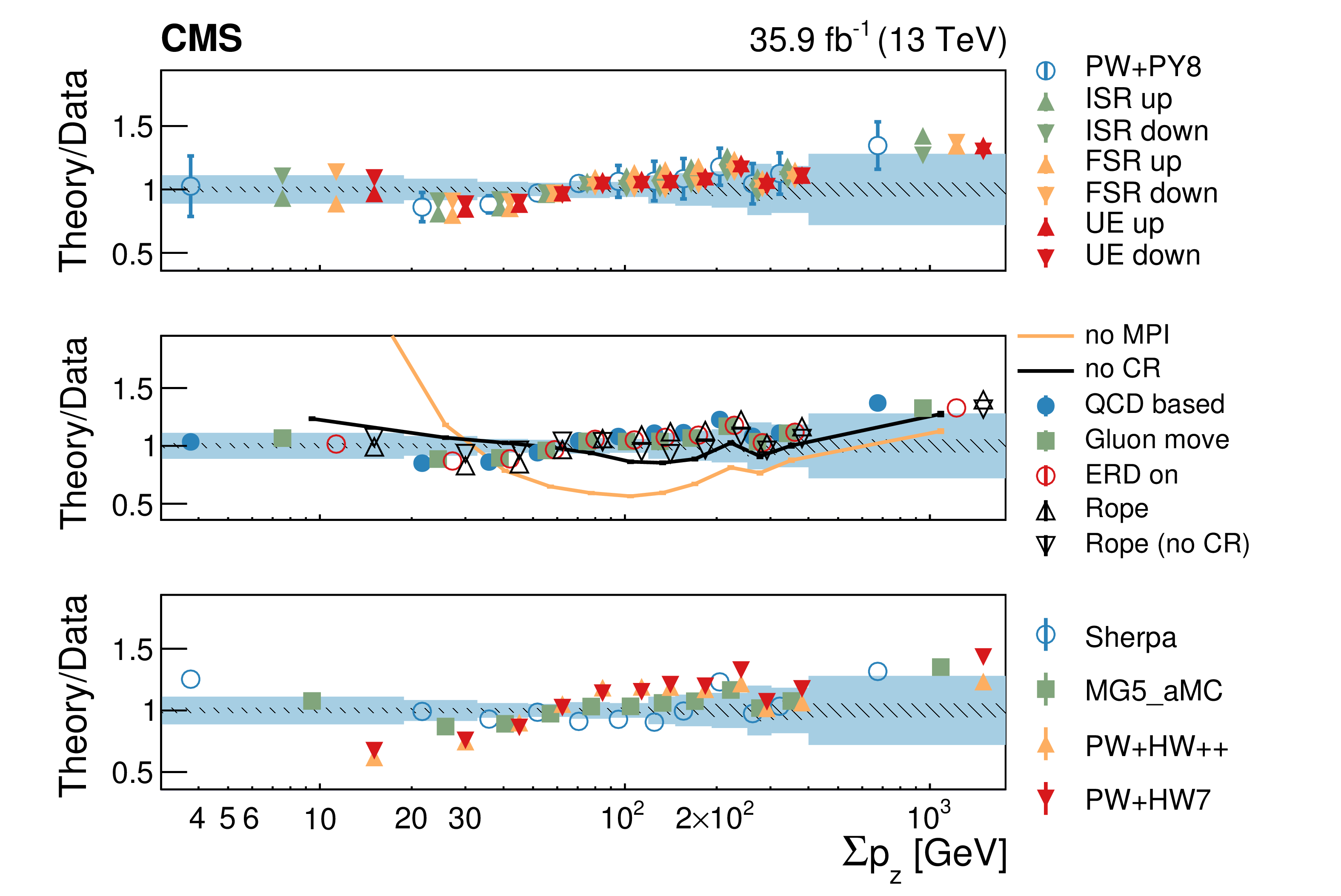
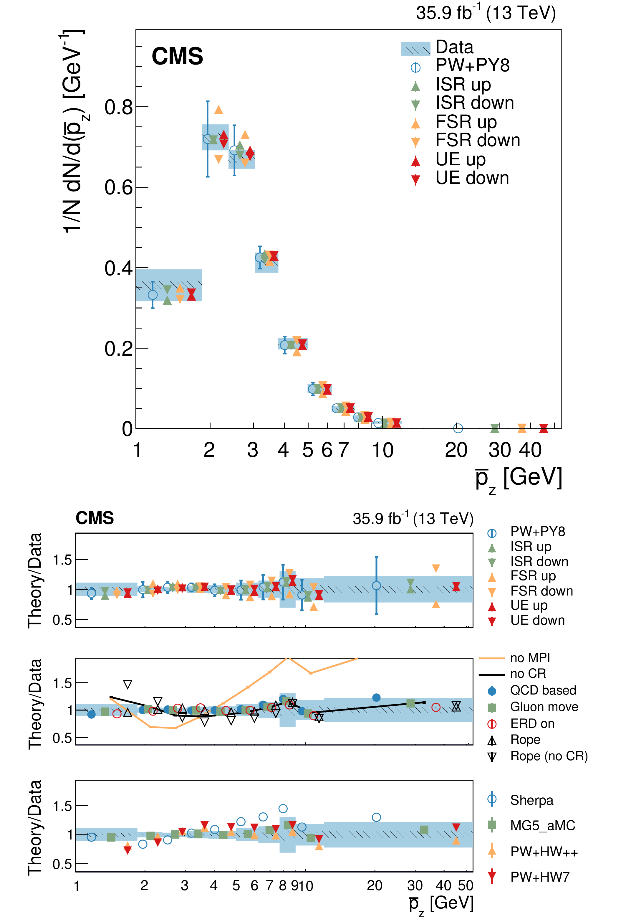
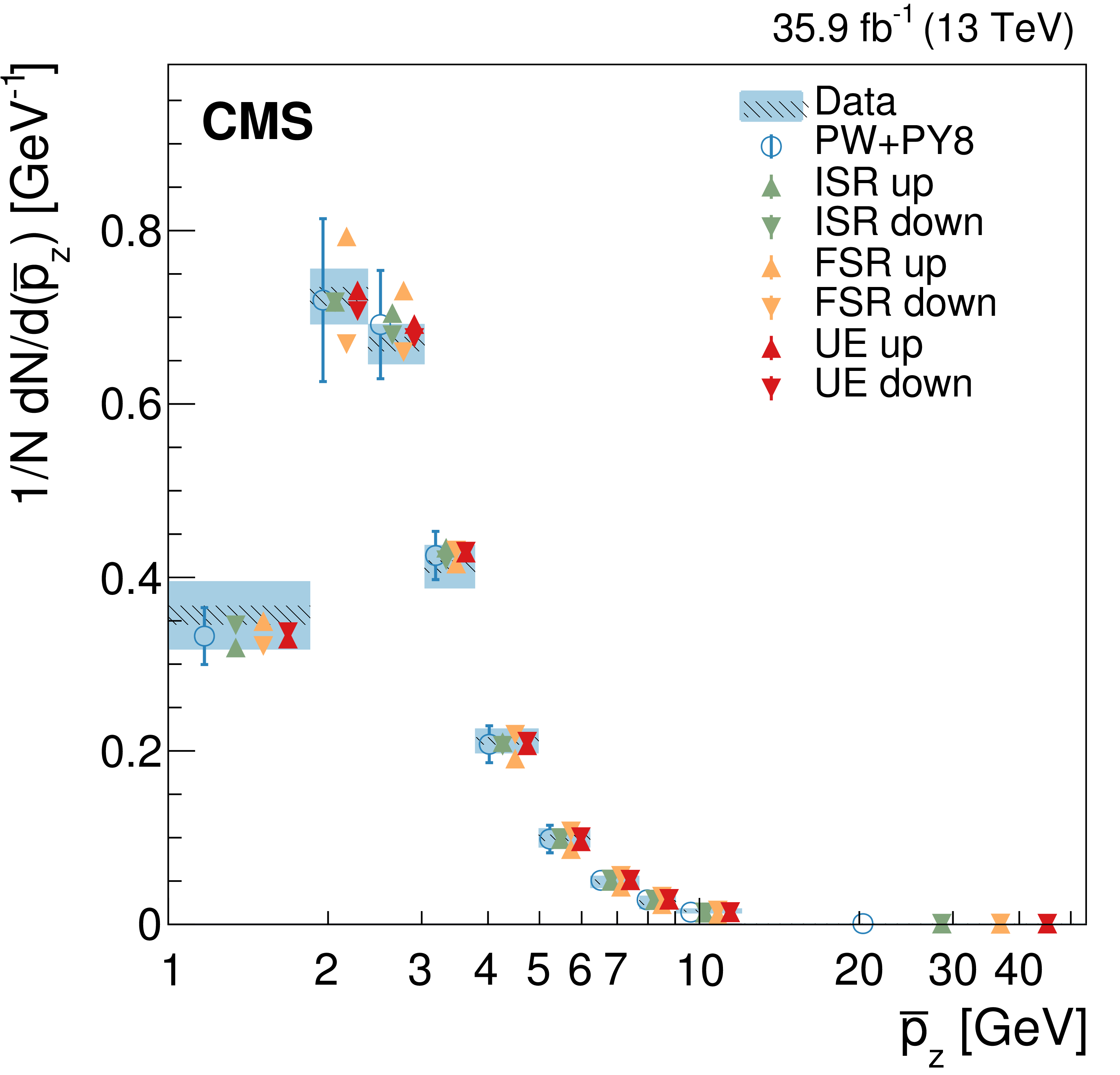
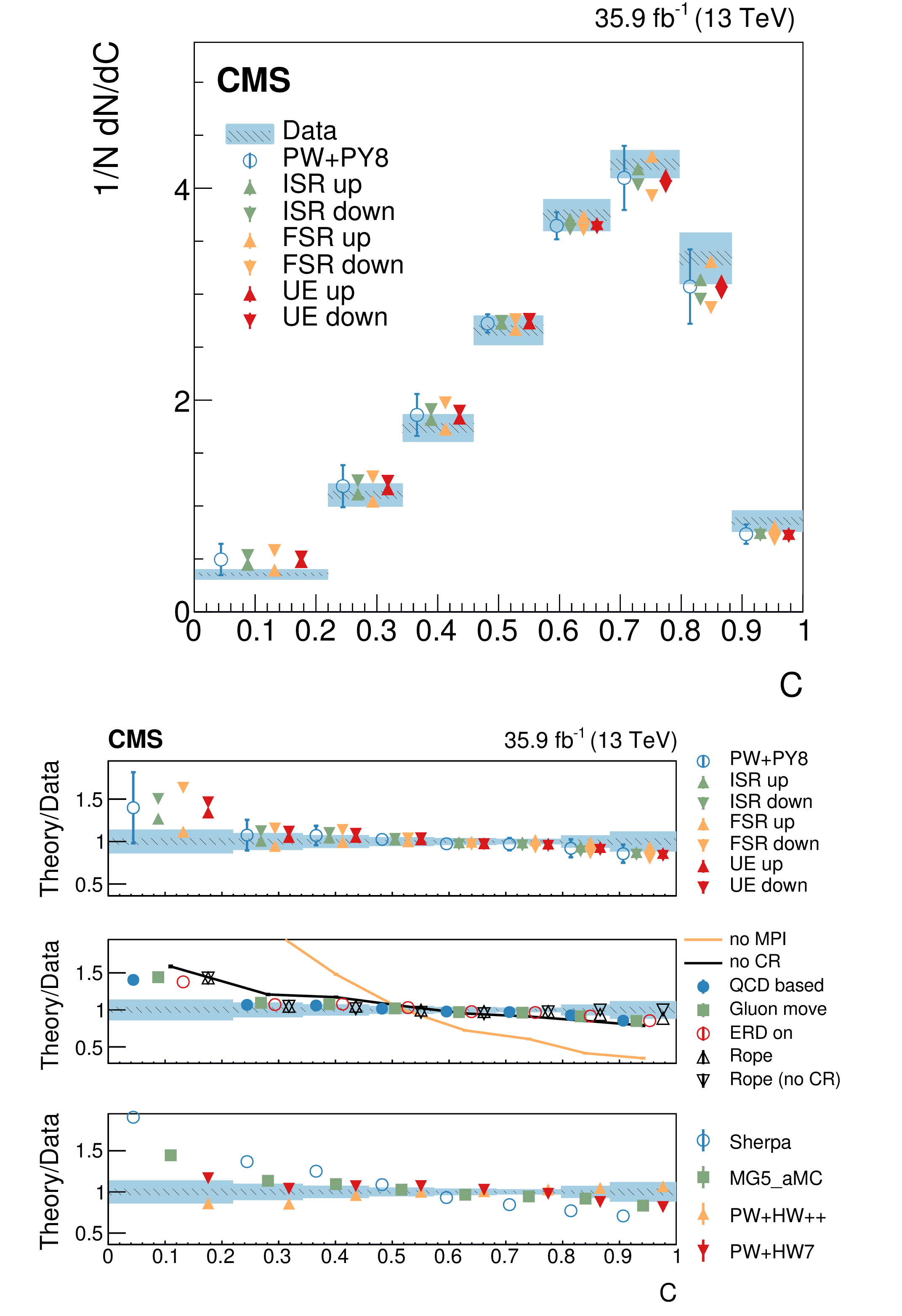
The normalized differential cross section as a function of $ {N_\text {ch}} $ is shown on the upper panel. The data (colored boxes) are compared to the nominal POWHEG+PYTHIA8 predictions and to the expectations obtained from varied $ {\alpha _S} ^\text {ISR}(M_ {\mathrm {Z}})$ or $ {\alpha _S} ^\text {FSR}(M_ {\mathrm {Z}})$ POWHEG+PYTHIA8 setups (markers). The different panels on the lower display show the ratio between each model tested (see text) and the data. In both cases the shaded (hatched) band represents the total (statistical) uncertainty of the data, while the error bars represent either the total uncertainty of the POWHEG+PYTHIA8 setup, computed as described in the text, or the statistical uncertainty of the other MC simulation setups. |
png pdf |
Figure 4-a:
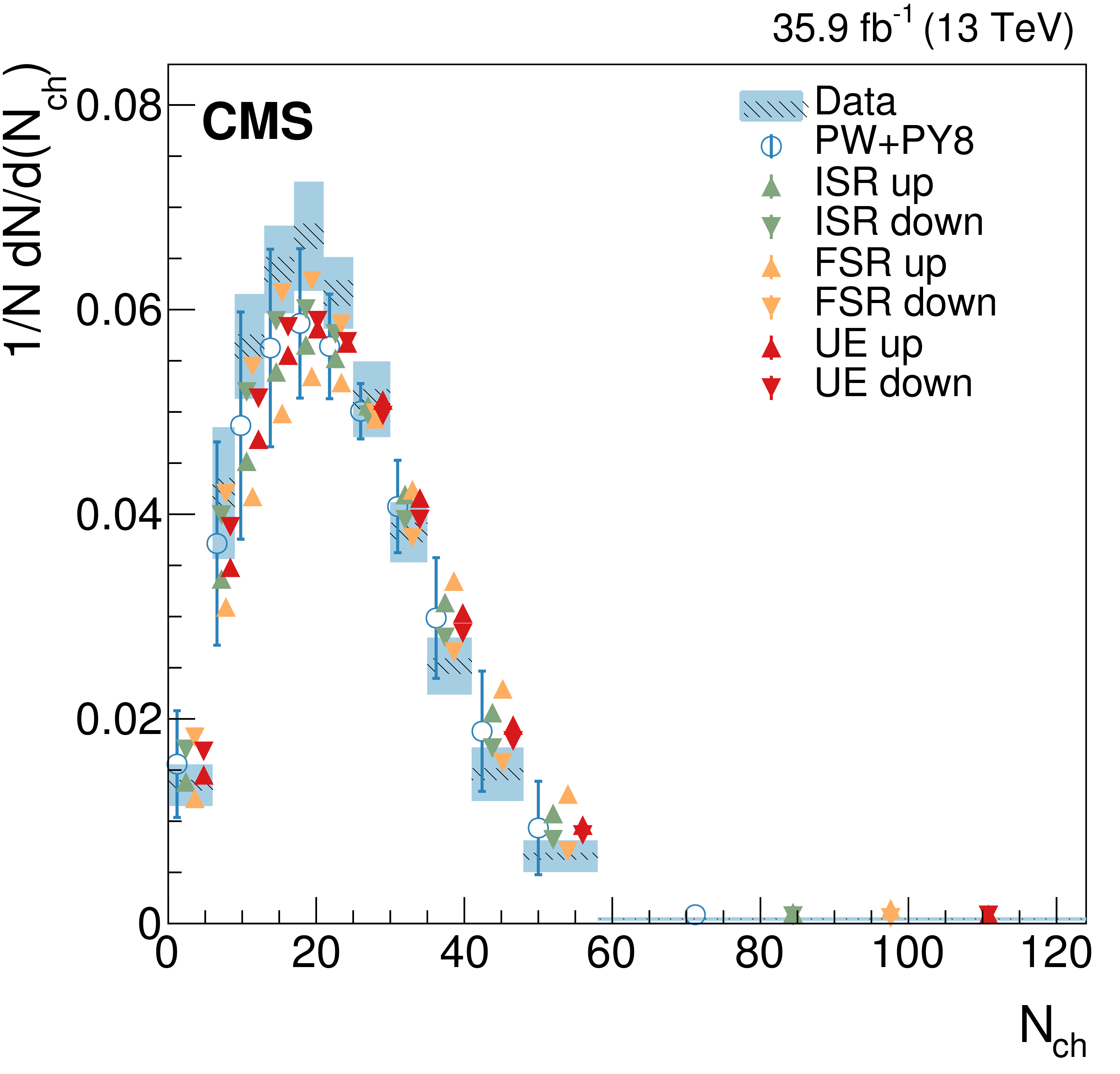
The normalized differential cross section as a function of $ {N_\text {ch}} $ is shown. The data (colored boxes) are compared to the nominal POWHEG+PYTHIA8 predictions and to the expectations obtained from varied $ {\alpha _S} ^\text {ISR}(M_ {\mathrm {Z}})$ or $ {\alpha _S} ^\text {FSR}(M_ {\mathrm {Z}})$ POWHEG+PYTHIA8 setups (markers). |
png pdf |
Figure 4-b:
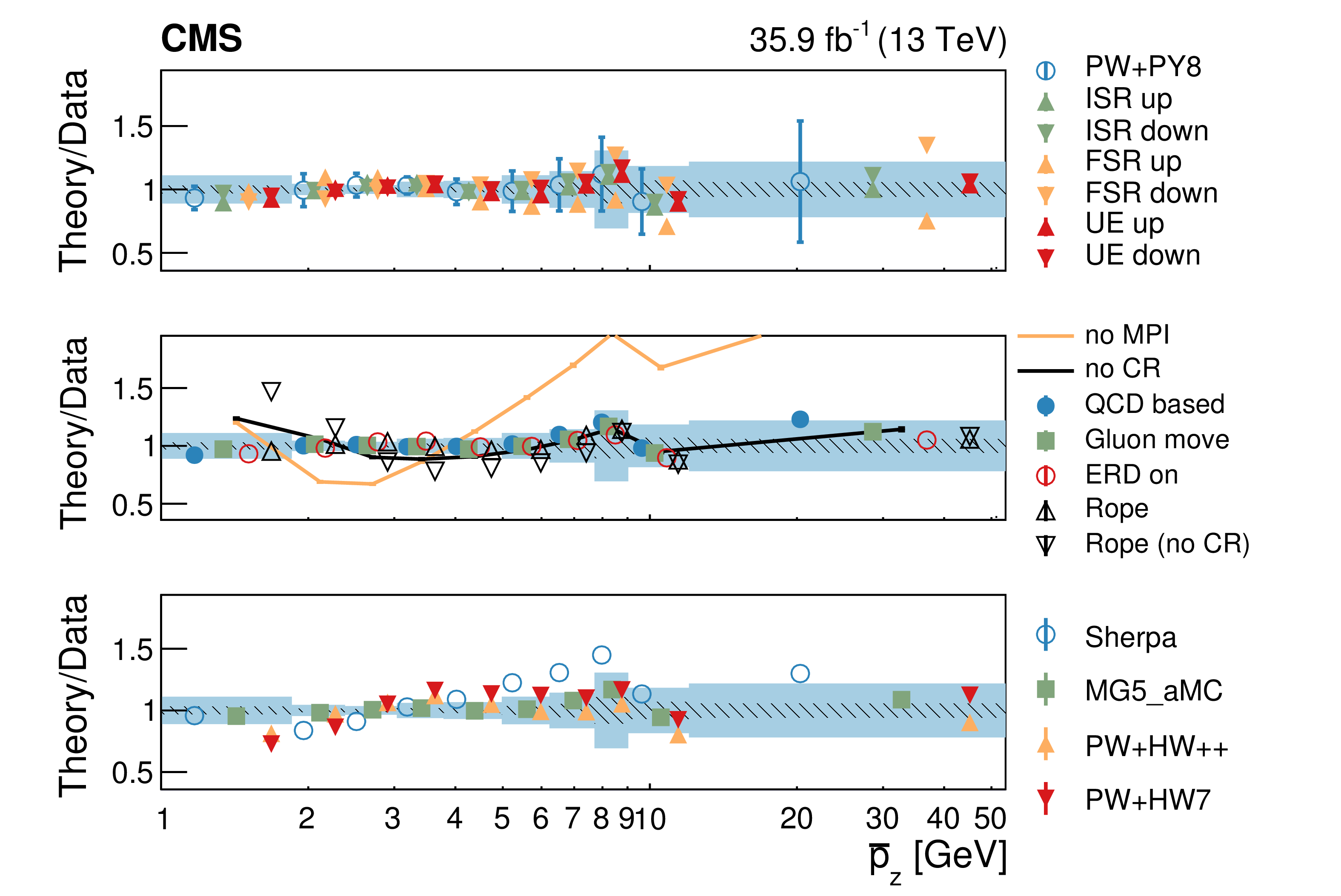
The different panels show the ratio between each model tested (see text) and the data. In both cases the shaded (hatched) band represents the total (statistical) uncertainty of the data, while the error bars represent either the total uncertainty of the POWHEG+PYTHIA8 setup, computed as described in the text, or the statistical uncertainty of the other MC simulation setups. |
png pdf |
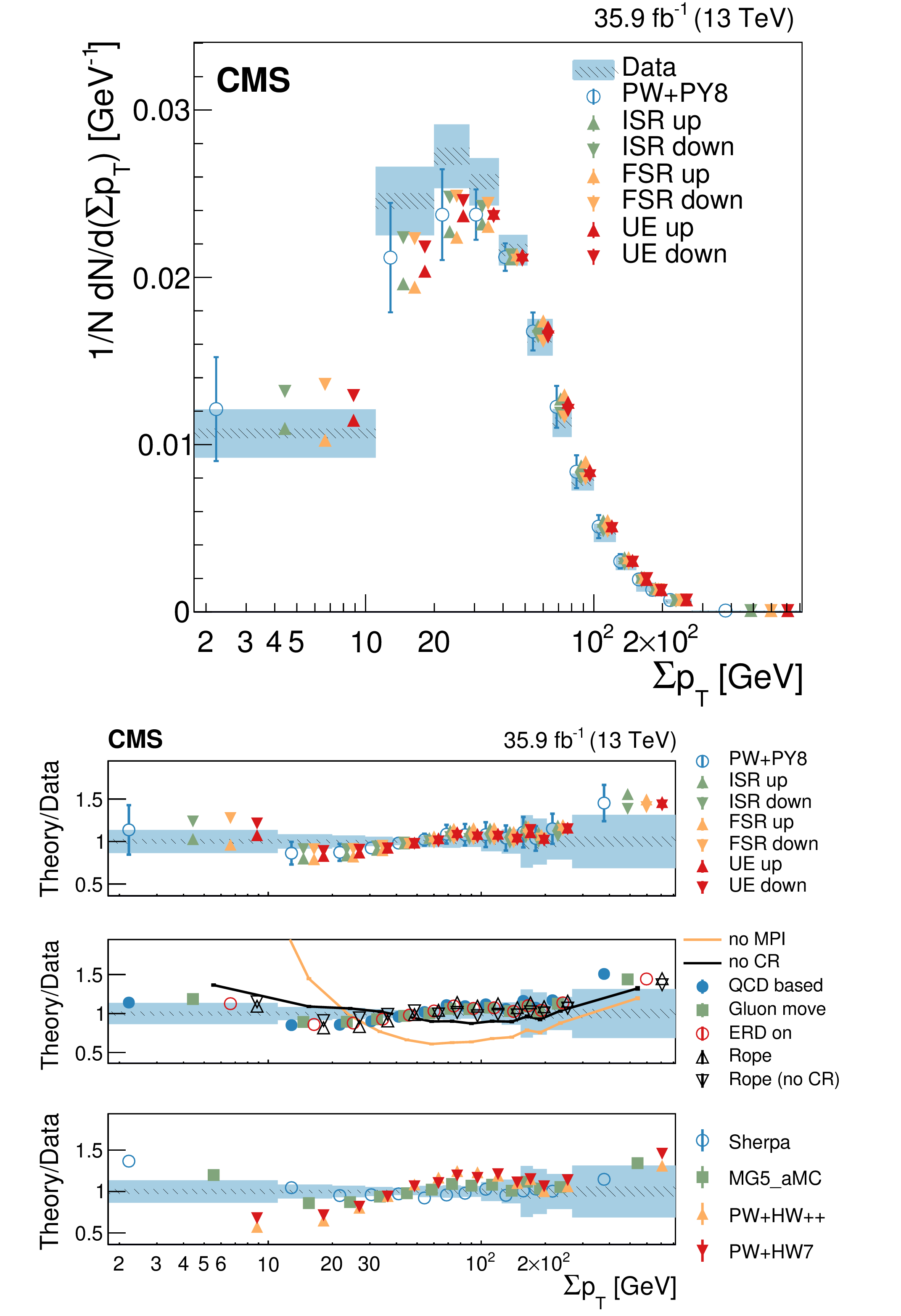
Figure 5:
Normalized differential cross section as function of $\Sigma {p_{\mathrm {T}}}$ , compared to the predictions of different models. The conventions of Fig. 4 are used. |
png pdf |
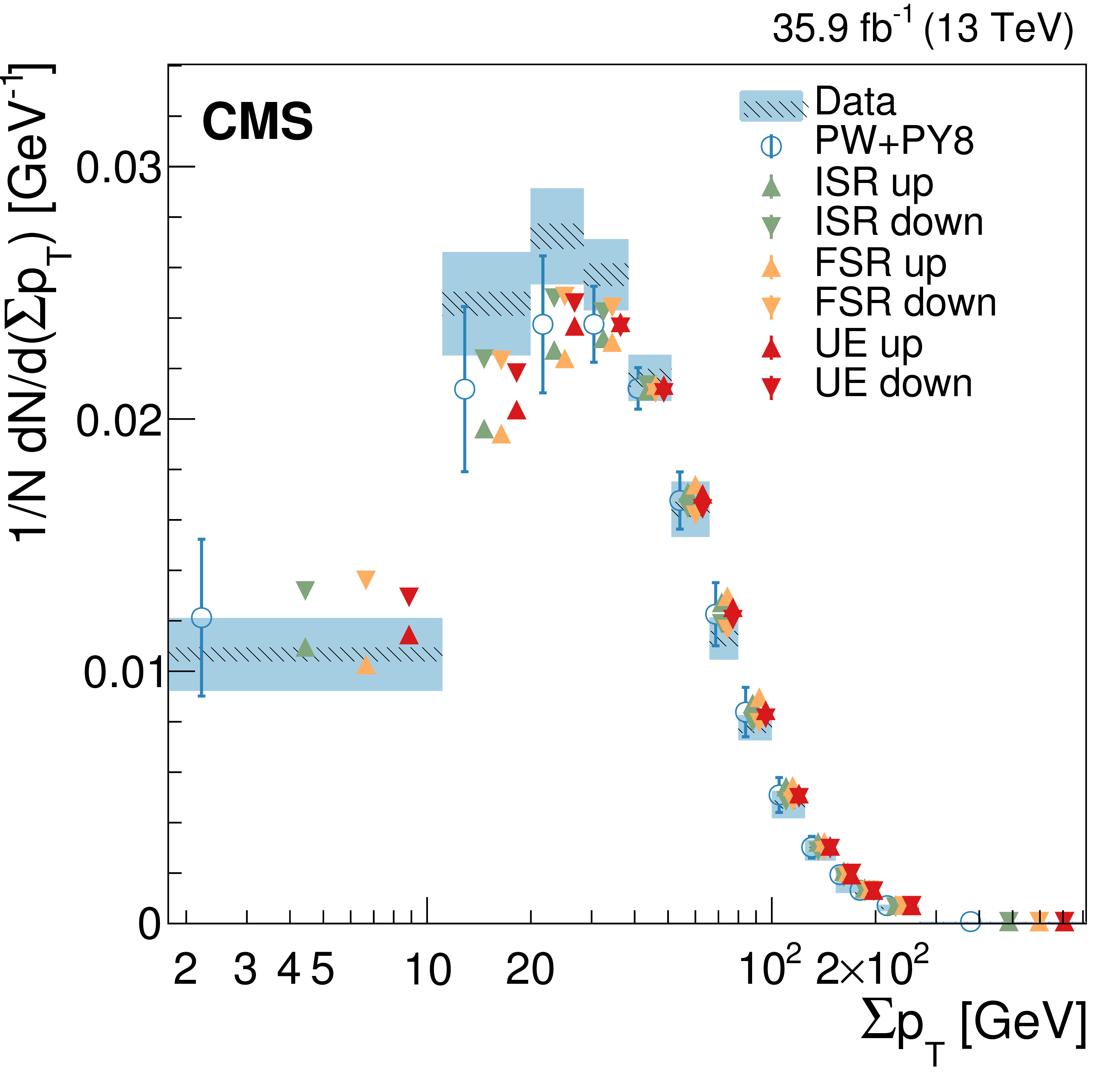
Figure 5-a:
Normalized differential cross section as function of $\Sigma {p_{\mathrm {T}}}$ , compared to the predictions of different models. The conventions of Fig. 4 are used. |
png pdf |
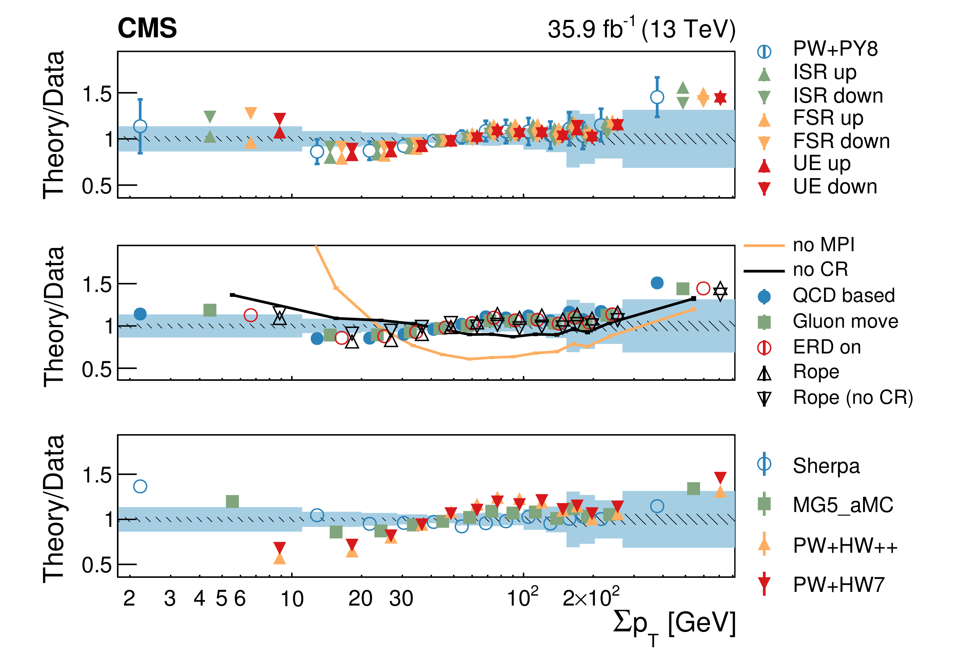
Figure 5-b:
Normalized differential cross section as function of $\Sigma {p_{\mathrm {T}}}$ , compared to the predictions of different models. The conventions of Fig. 4 are used. |
png pdf |
Figure 6:
Normalized differential cross section as function of $ {\overline {{p_{\mathrm {T}}}}} $, compared to the predictions of different models. The conventions of Fig. 4 are used. |
png pdf |
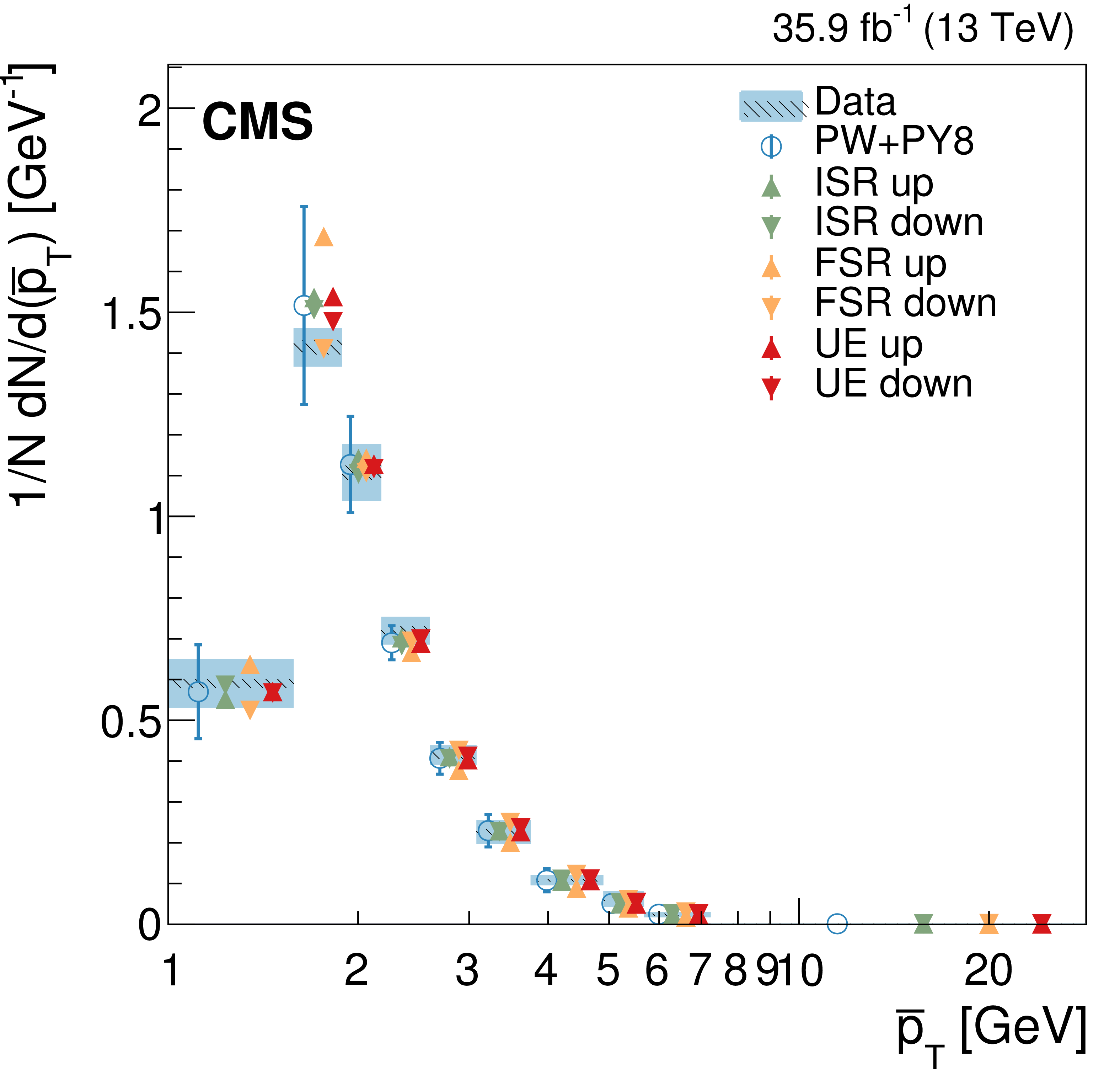
Figure 6-a:
Normalized differential cross section as function of $ {\overline {{p_{\mathrm {T}}}}} $, compared to the predictions of different models. The conventions of Fig. 4 are used. |
png pdf |
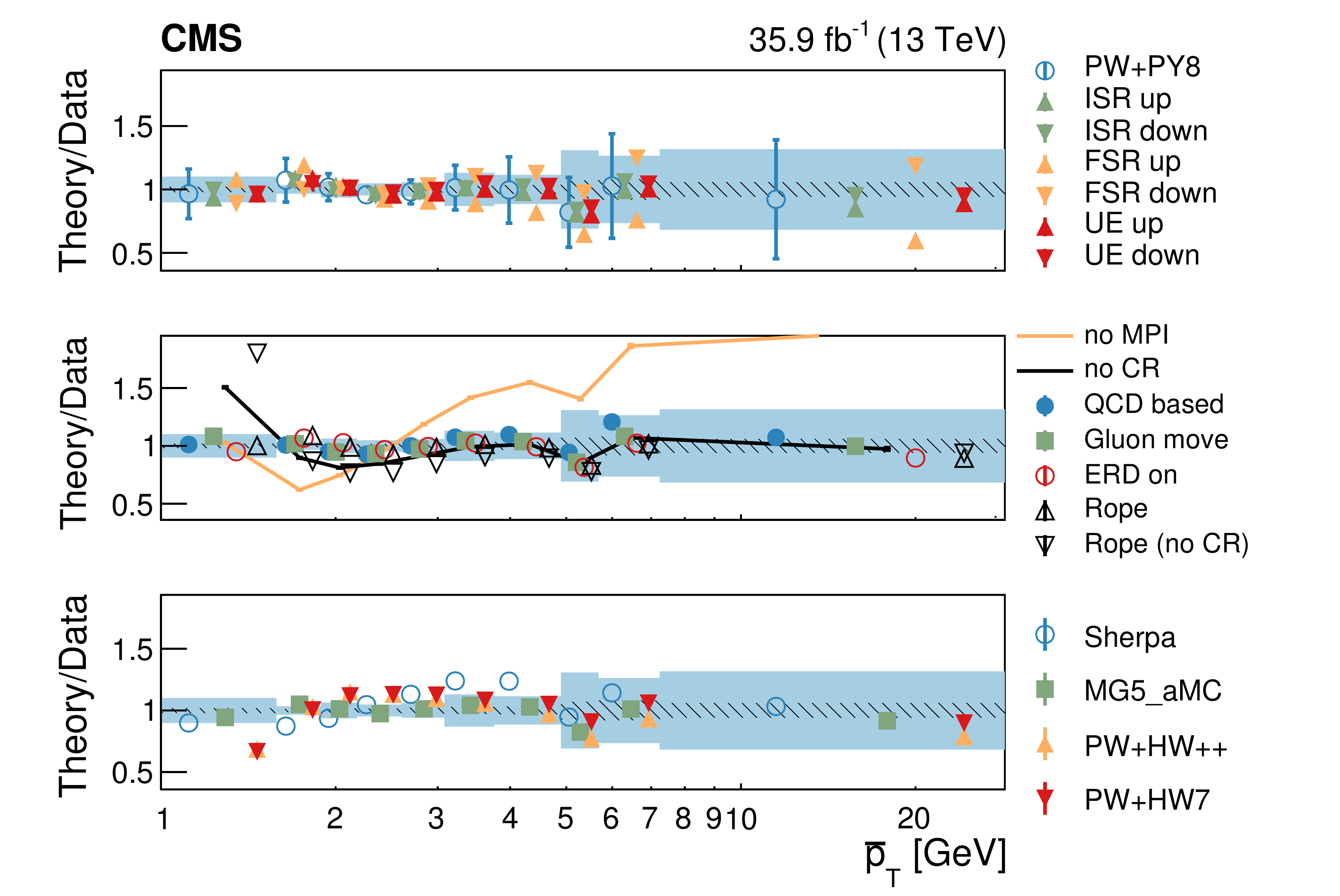
Figure 6-b:
Normalized differential cross section as function of $ {\overline {{p_{\mathrm {T}}}}} $, compared to the predictions of different models. The conventions of Fig. 4 are used. |

png pdf |
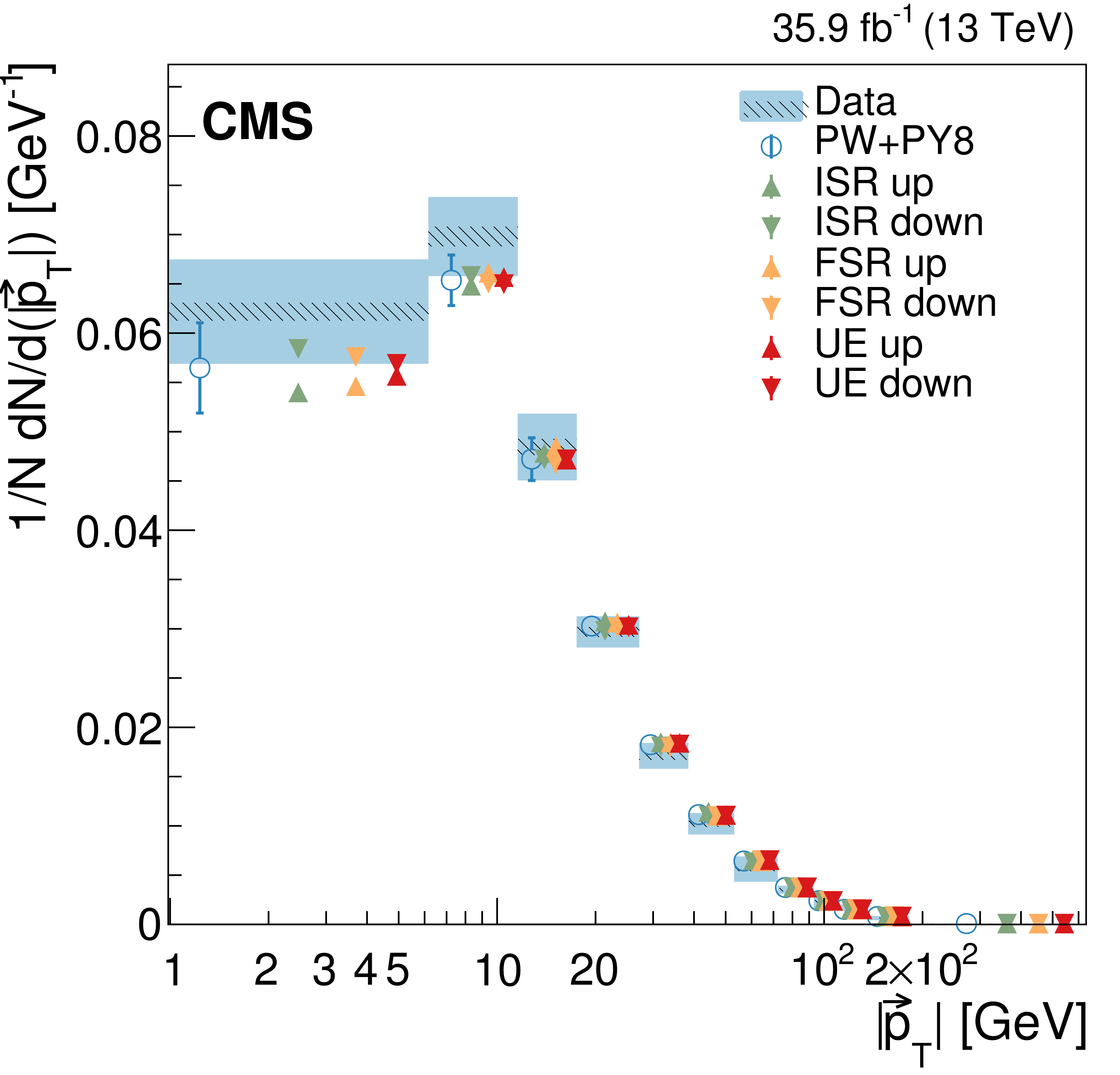
Figure 7:
Normalized differential cross section as function of $ {{| {\vec{p}_{\mathrm {T}}} |}} $, compared to the predictions of different models. The conventions of Fig. 4 are used. |
png pdf |
Figure 7-a:
Normalized differential cross section as function of $ {{| {\vec{p}_{\mathrm {T}}} |}} $, compared to the predictions of different models. The conventions of Fig. 4 are used. |
png pdf |
Figure 7-b:
Normalized differential cross section as function of $ {{| {\vec{p}_{\mathrm {T}}} |}} $, compared to the predictions of different models. The conventions of Fig. 4 are used. |
png pdf |
Figure 8:
Normalized differential cross section as function of ${\Sigma p_{z}}$ , compared to the predictions of different models. The conventions of Fig. 4 are used. |

png pdf |
Figure 8-a:
Normalized differential cross section as function of ${\Sigma p_{z}}$ , compared to the predictions of different models. The conventions of Fig. 4 are used. |
png pdf |
Figure 8-b:
Normalized differential cross section as function of ${\Sigma p_{z}}$ , compared to the predictions of different models. The conventions of Fig. 4 are used. |
png pdf |
Figure 9:
Normalized differential cross section as function of ${\overline {p_z}}$ , compared to the predictions of different models. The conventions of Fig. 4 are used. |
png pdf |
Figure 9-a:
Normalized differential cross section as function of ${\overline {p_z}}$ , compared to the predictions of different models. The conventions of Fig. 4 are used. |
png pdf |
Figure 9-b:
Normalized differential cross section as function of ${\overline {p_z}}$ , compared to the predictions of different models. The conventions of Fig. 4 are used. |
png pdf |
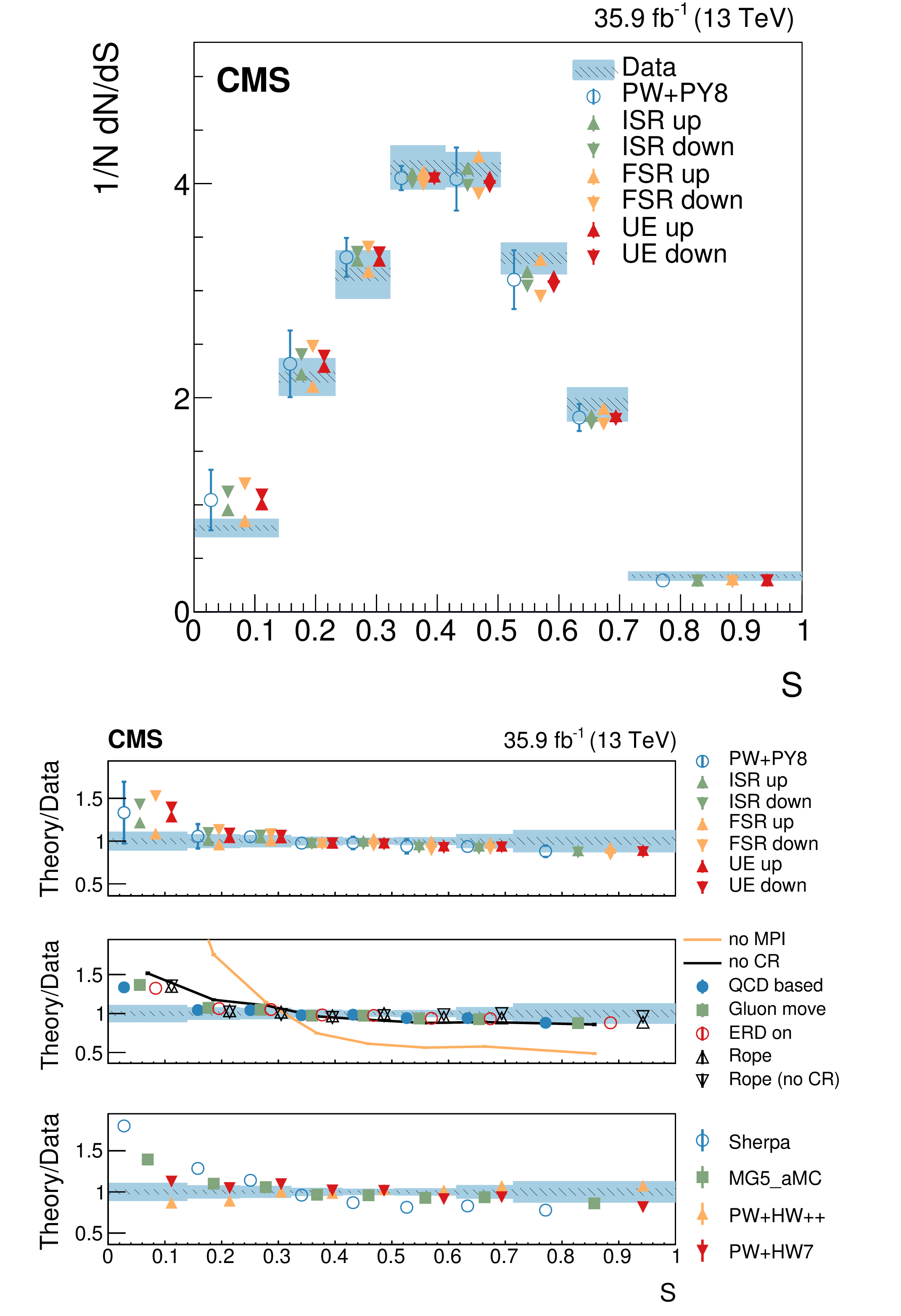
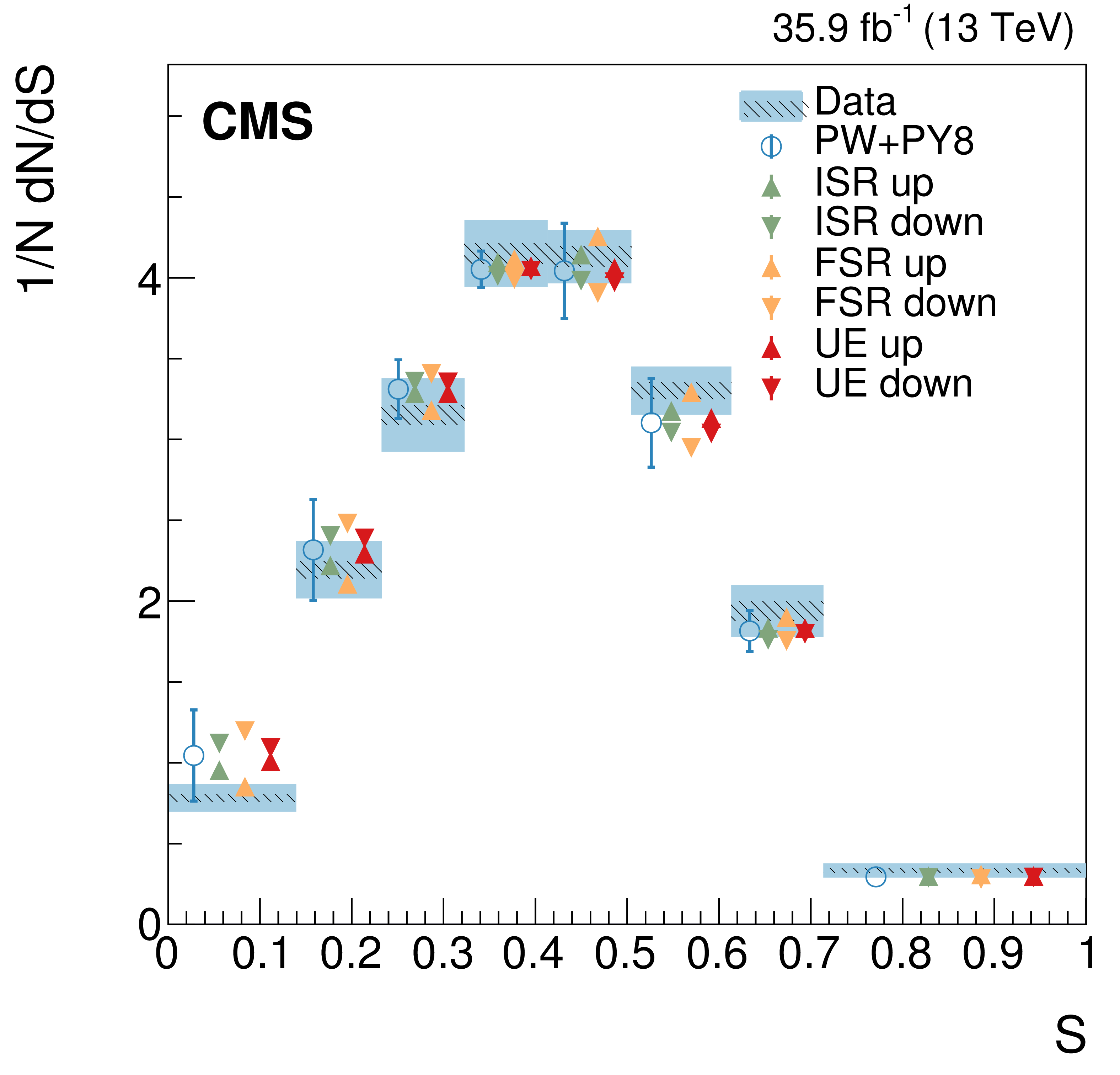
Figure 10:
Normalized differential cross section as function of the sphericity variable, compared to the predictions of different models. The conventions of Fig. 4 are used. |
png pdf |
Figure 10-a:
Normalized differential cross section as function of the sphericity variable, compared to the predictions of different models. The conventions of Fig. 4 are used. |
png pdf |
Figure 10-b:
Normalized differential cross section as function of the sphericity variable, compared to the predictions of different models. The conventions of Fig. 4 are used. |
png pdf |
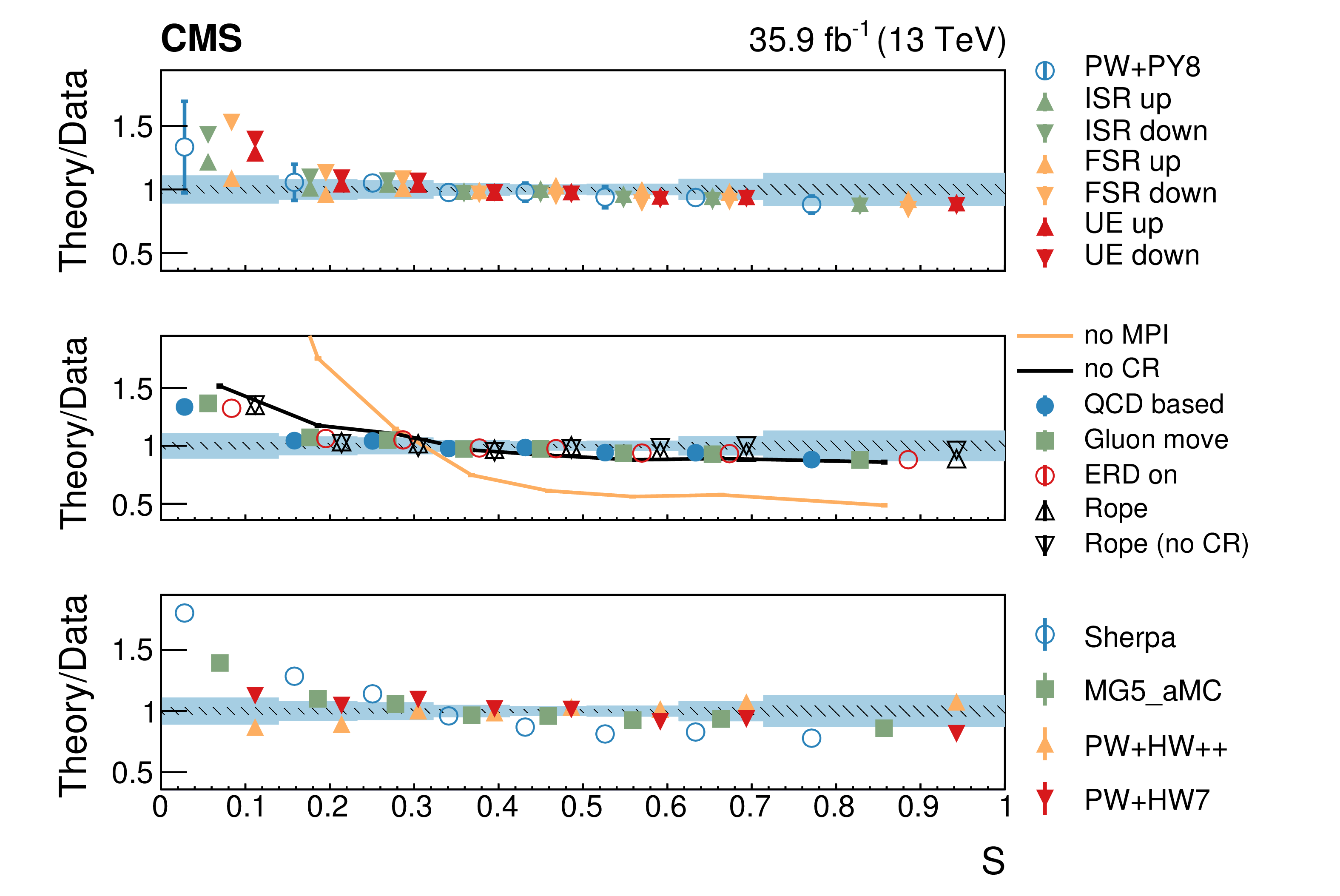
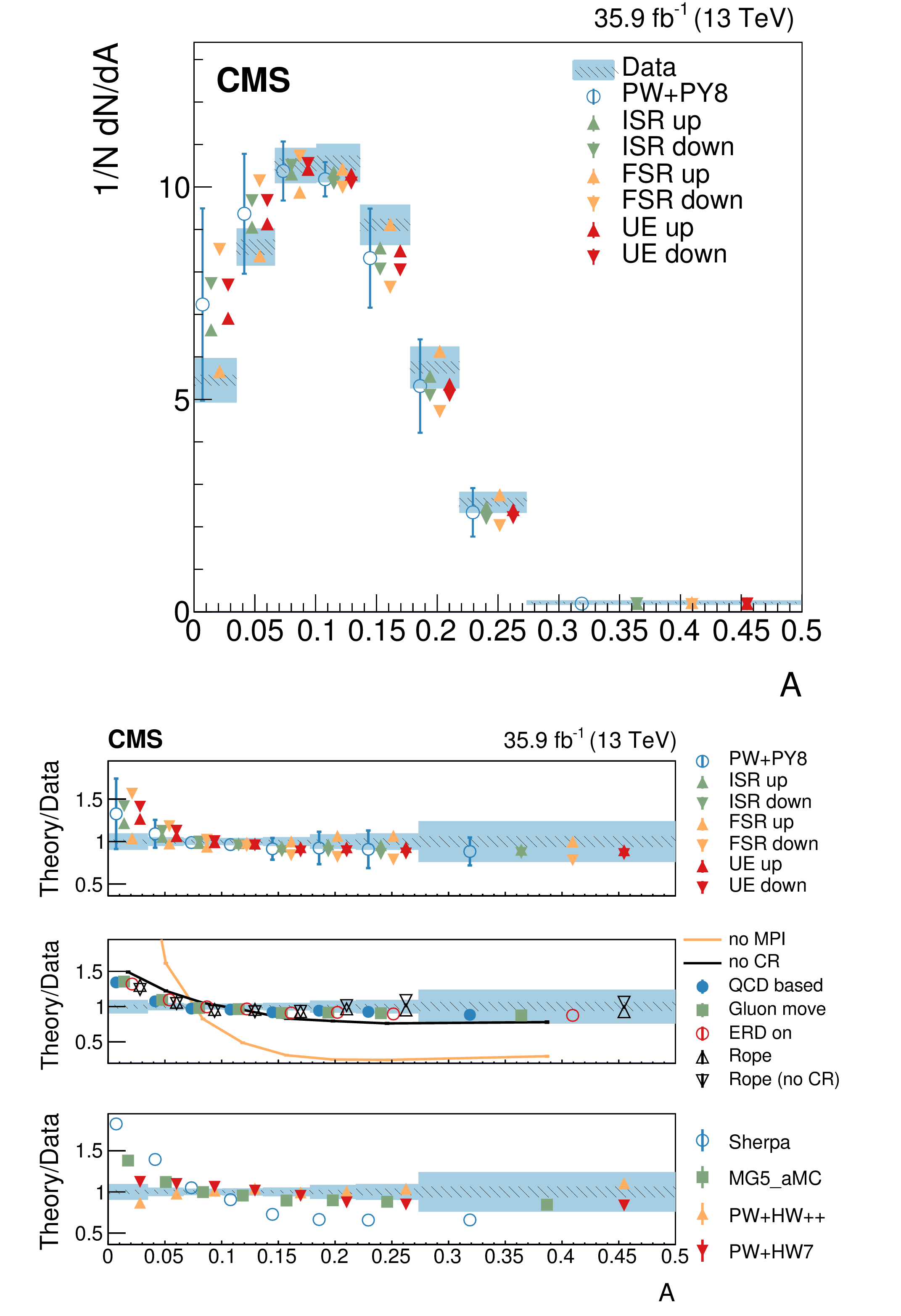
Figure 11:
Normalized differential cross section as function of the aplanarity variable, compared to the predictions of different models. The conventions of Fig. 4 are used. |
png pdf |
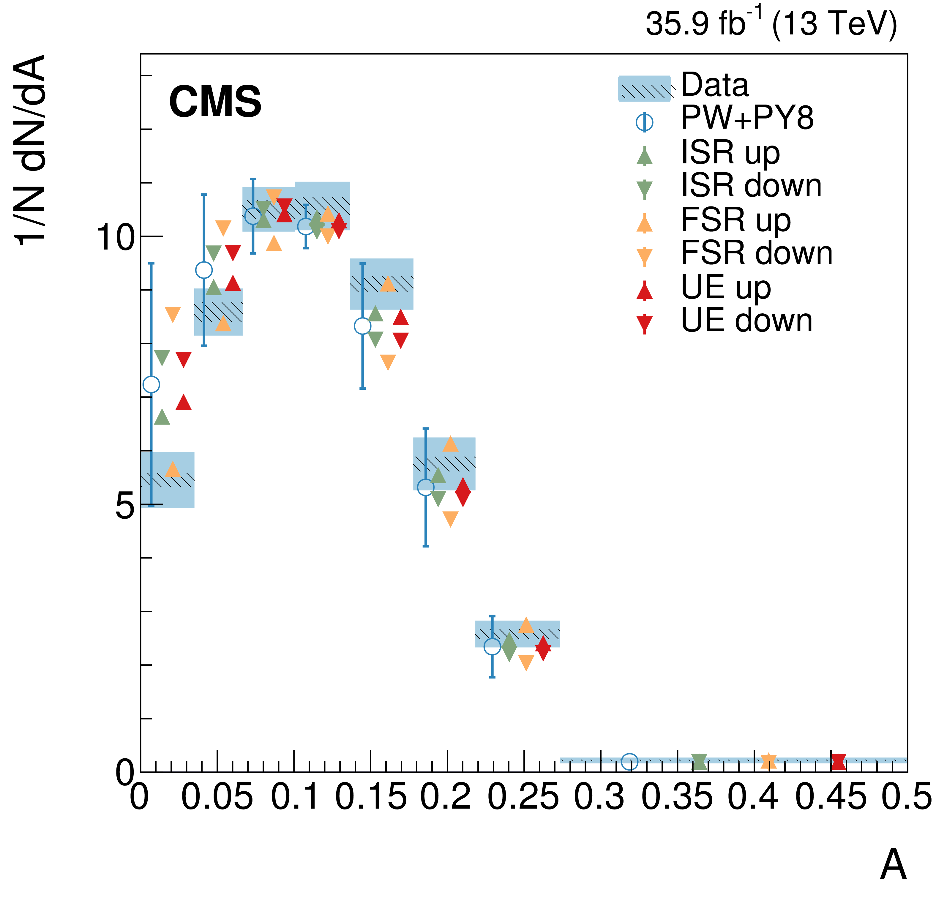
Figure 11-a:
Normalized differential cross section as function of the aplanarity variable, compared to the predictions of different models. The conventions of Fig. 4 are used. |
png pdf |
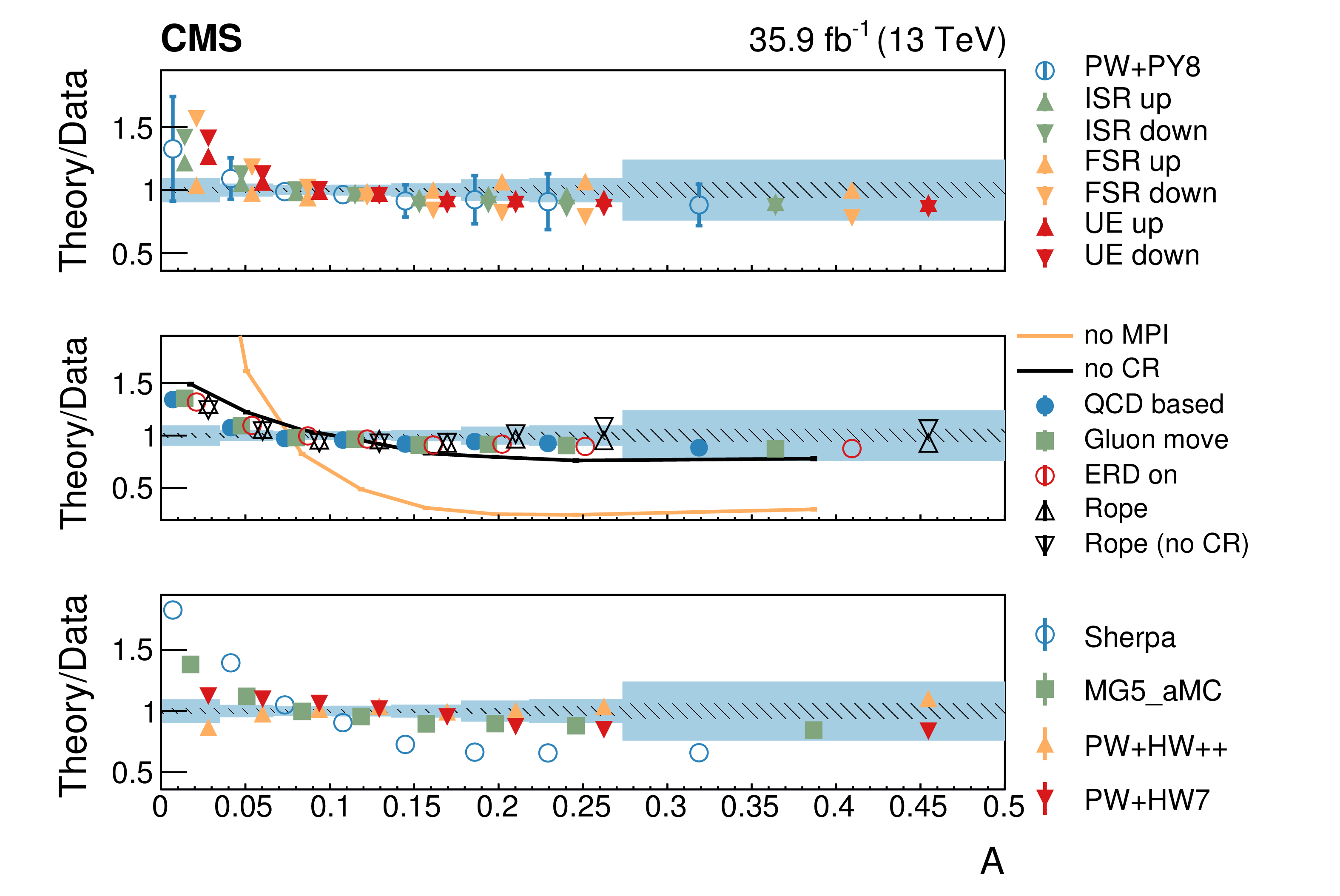
Figure 11-b:
Normalized differential cross section as function of the aplanarity variable, compared to the predictions of different models. The conventions of Fig. 4 are used. |
png pdf |
Figure 12:
Normalized differential cross section as function of the $C$ variable, compared to the predictions of different models. The conventions of Fig. 4 are used. |
png pdf |
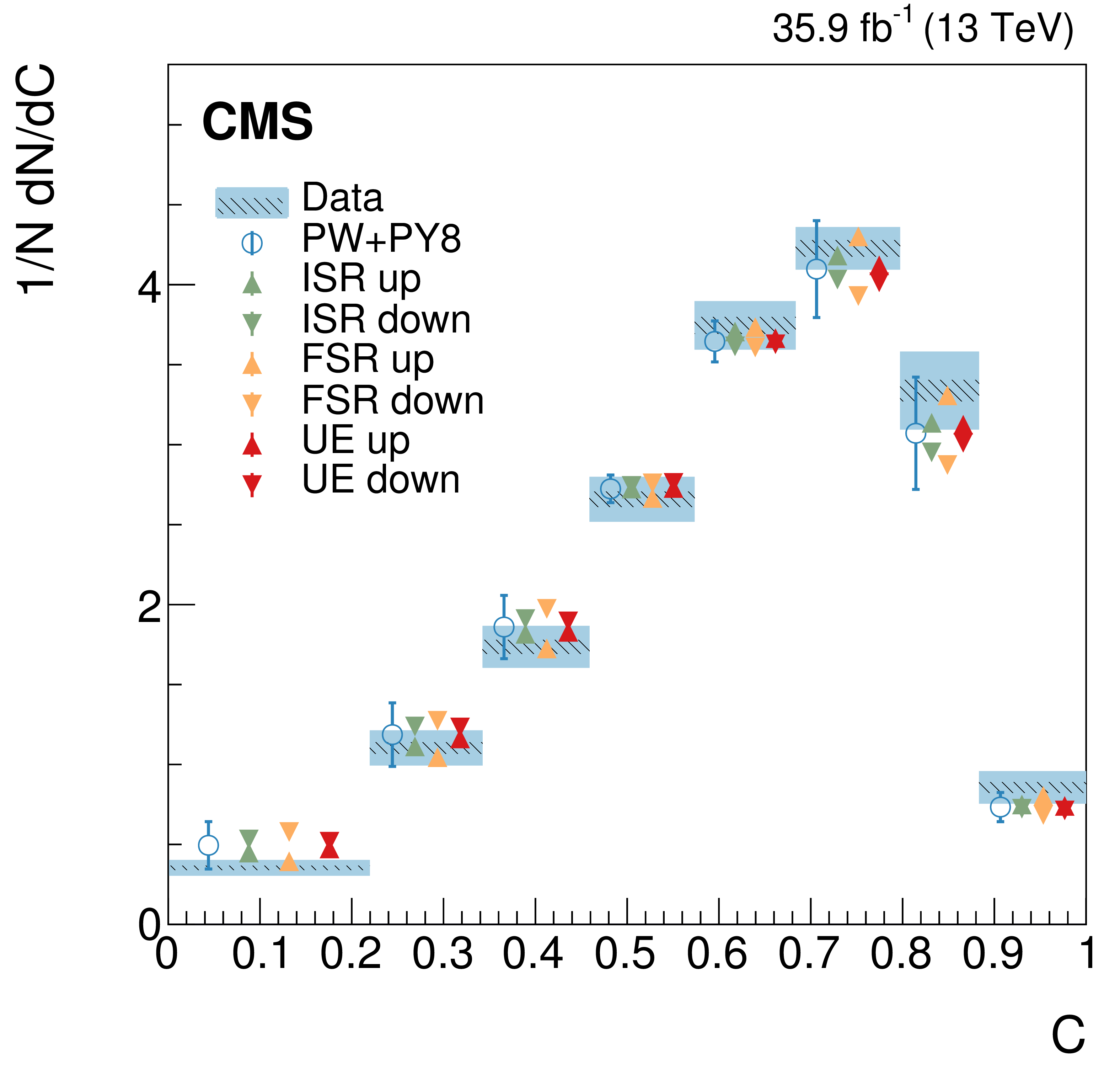
Figure 12-a:
Normalized differential cross section as function of the $C$ variable, compared to the predictions of different models. The conventions of Fig. 4 are used. |
png pdf |
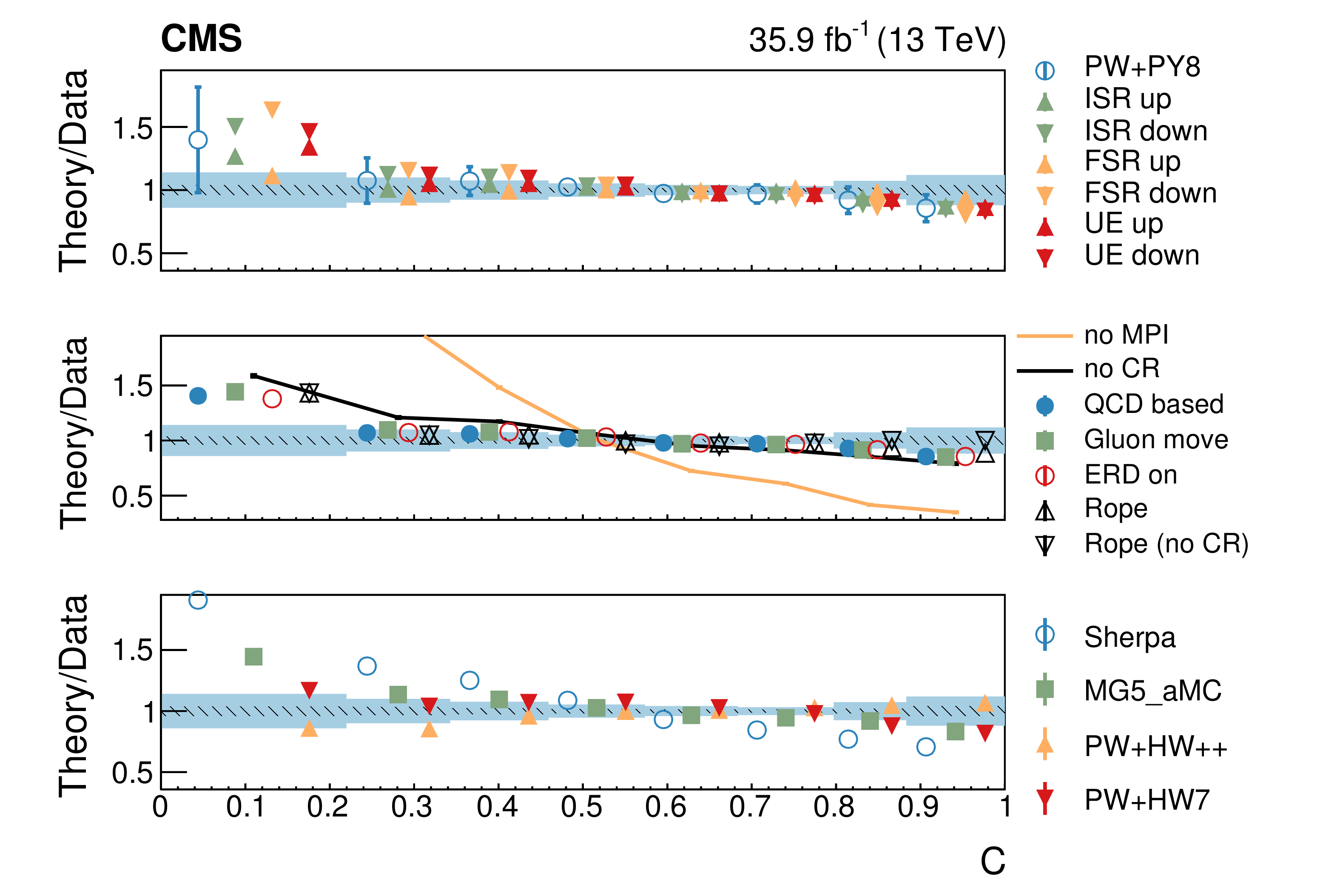
Figure 12-b:
Normalized differential cross section as function of the $C$ variable, compared to the predictions of different models. The conventions of Fig. 4 are used. |
png pdf |
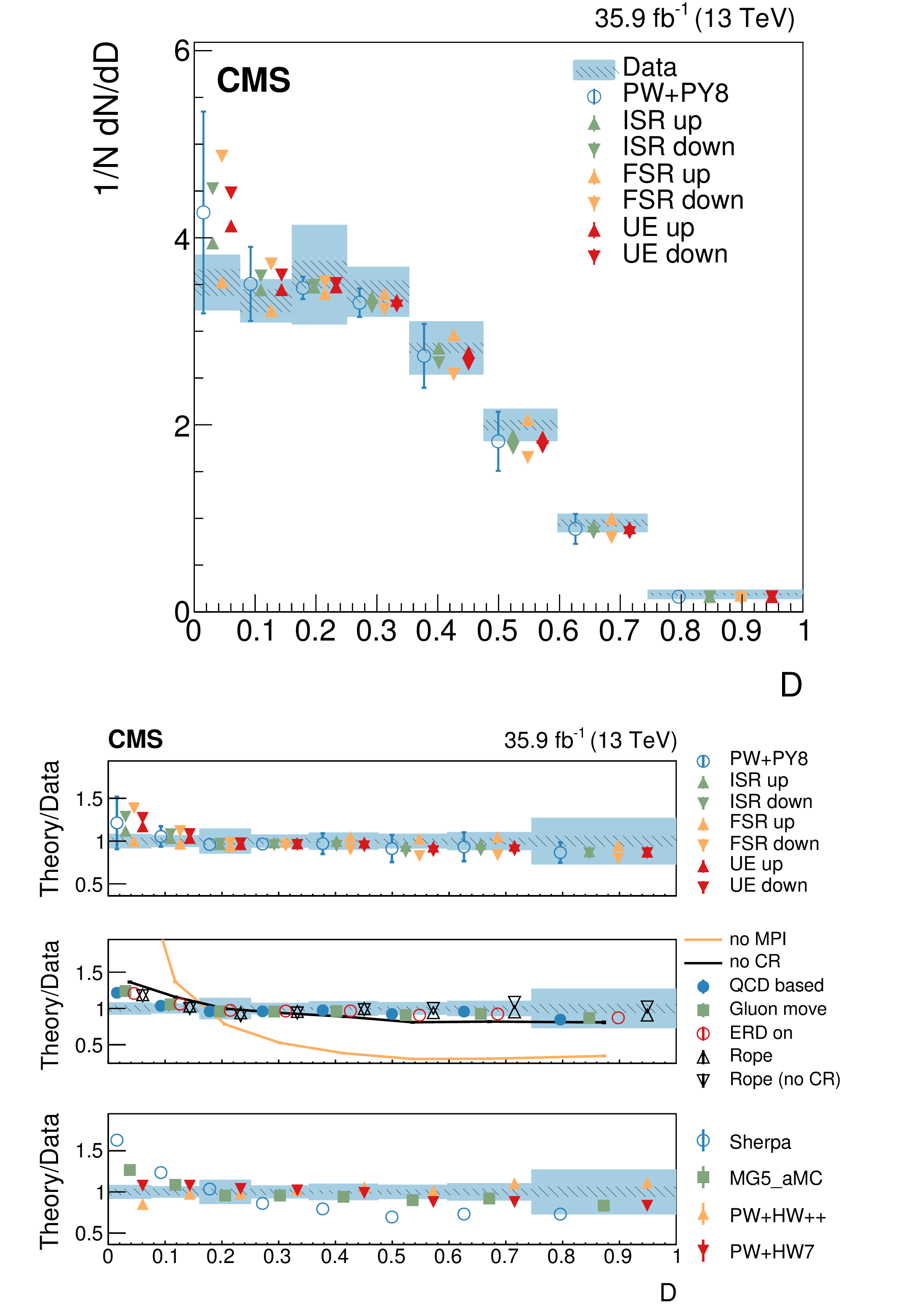
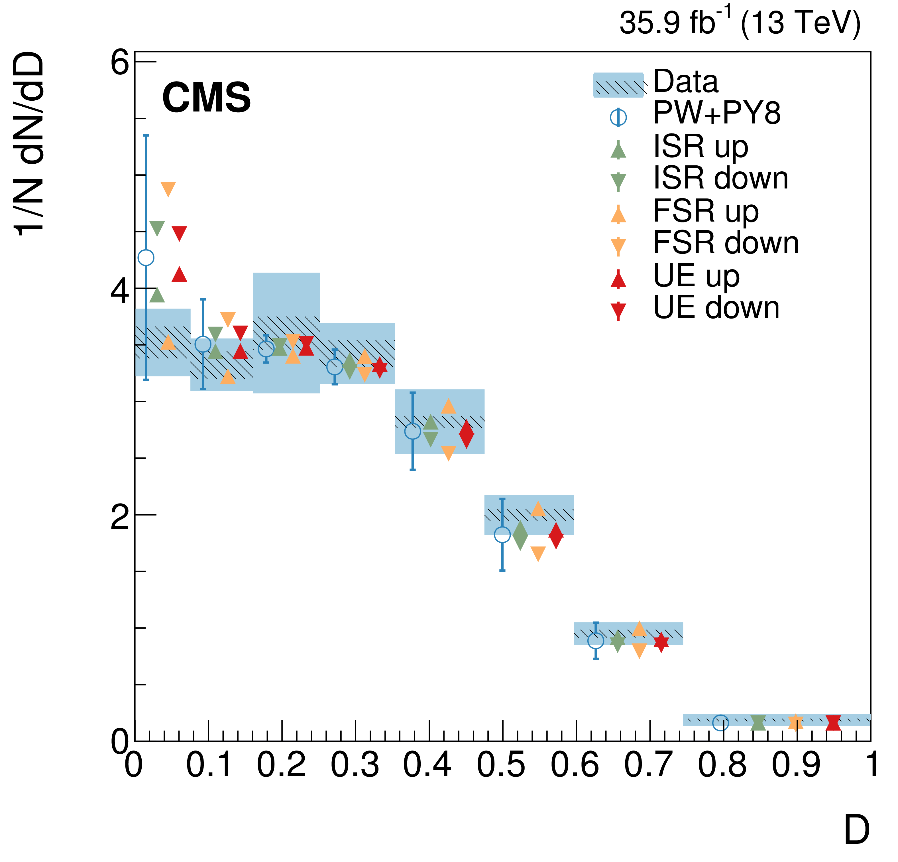
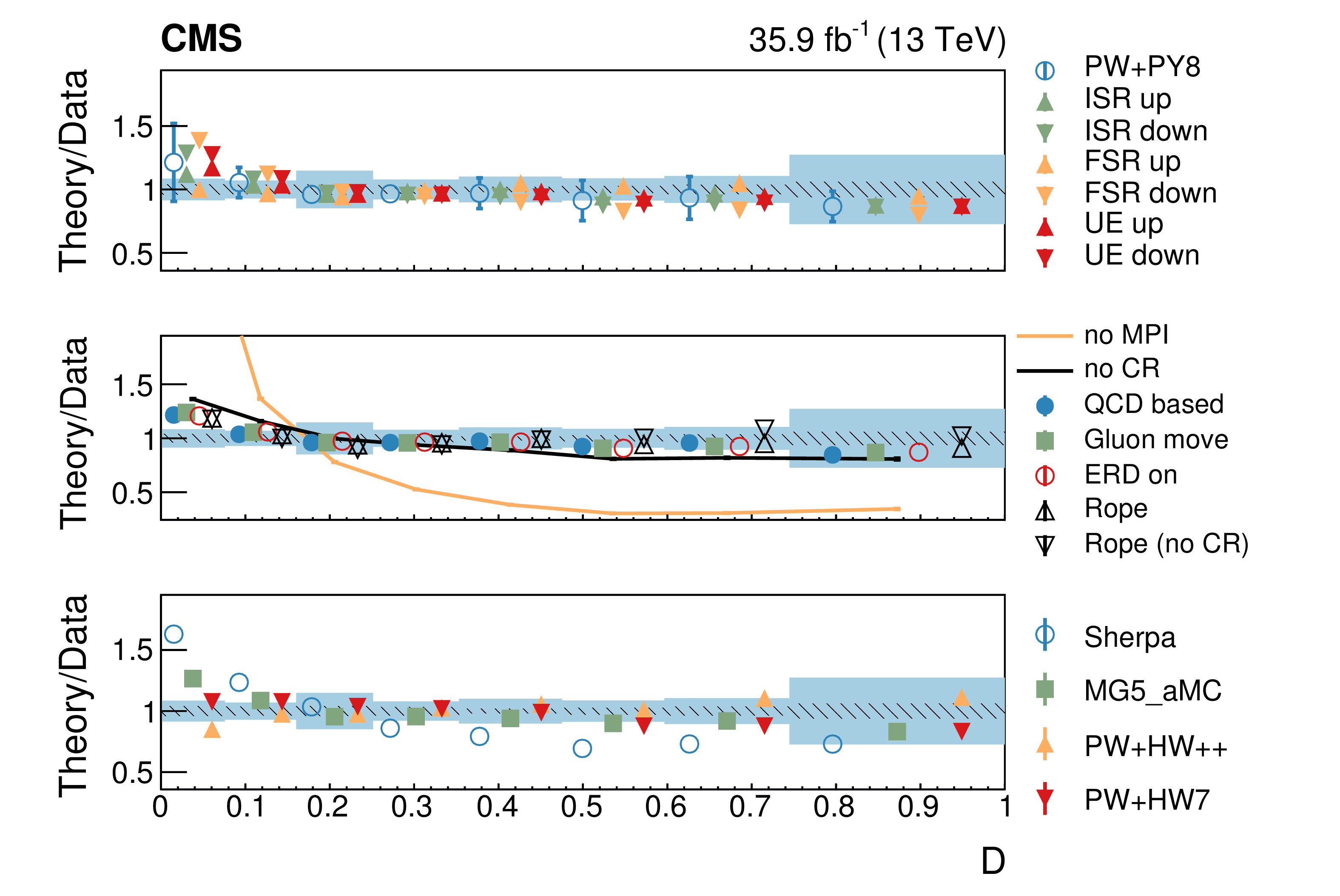
Figure 13:
Normalized differential cross section as function of the $D$ variable, compared to the predictions of different models. The conventions of Fig. 4 are used. |
png pdf |
Figure 13-a:
Normalized differential cross section as function of the $D$ variable, compared to the predictions of different models. The conventions of Fig. 4 are used. |
png pdf |
Figure 13-b:
Normalized differential cross section as function of the $D$ variable, compared to the predictions of different models. The conventions of Fig. 4 are used. |
png pdf |
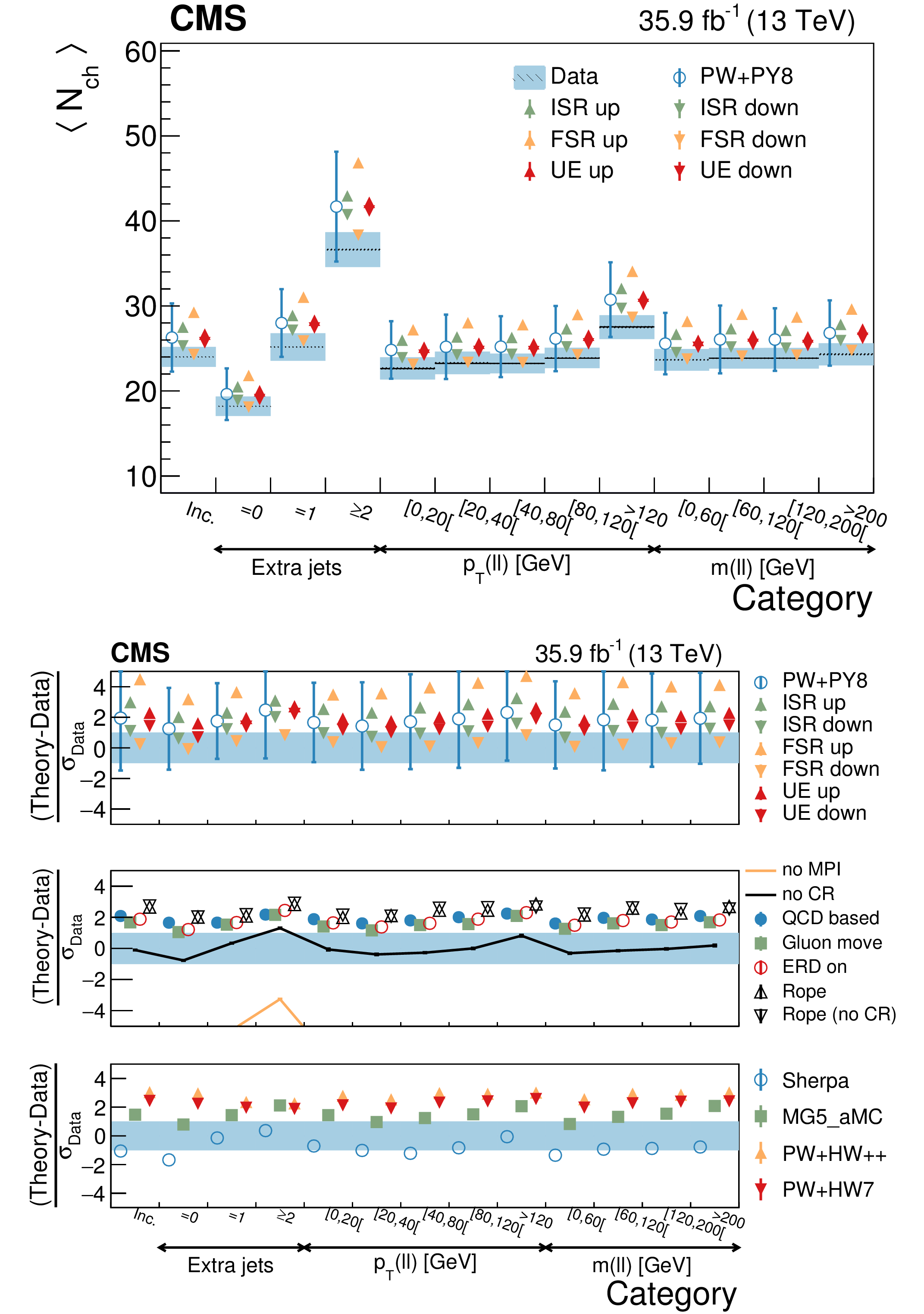
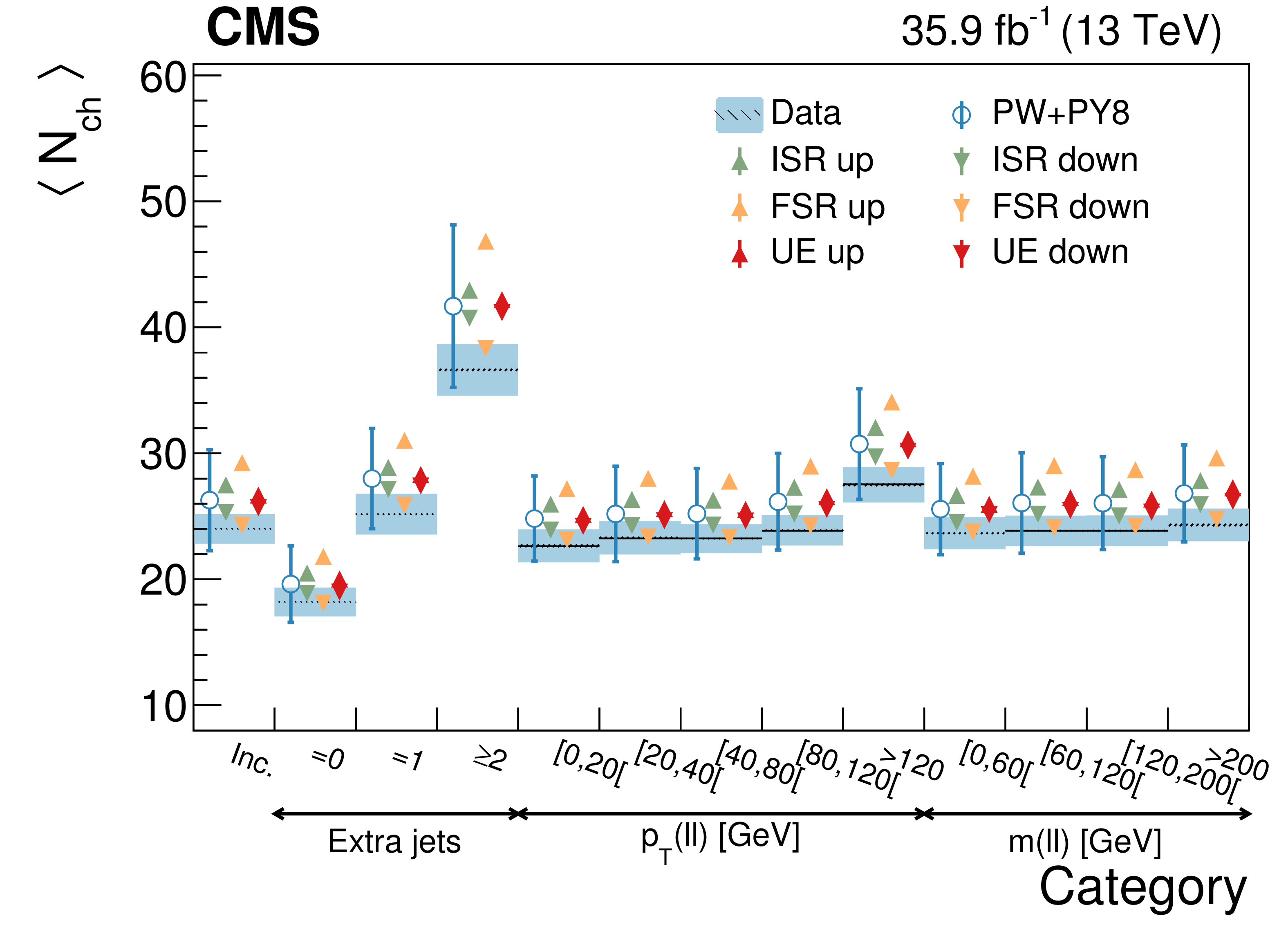
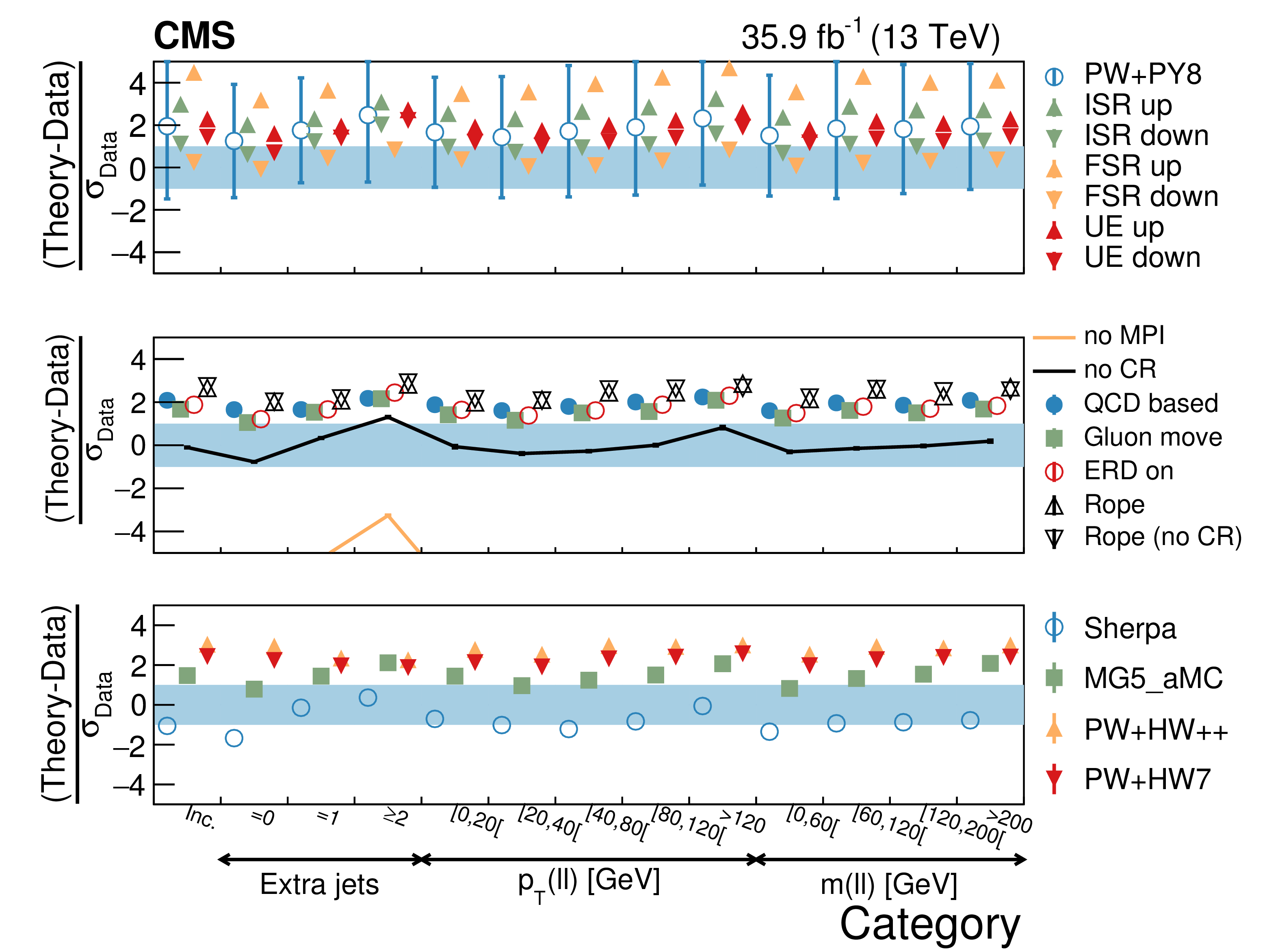
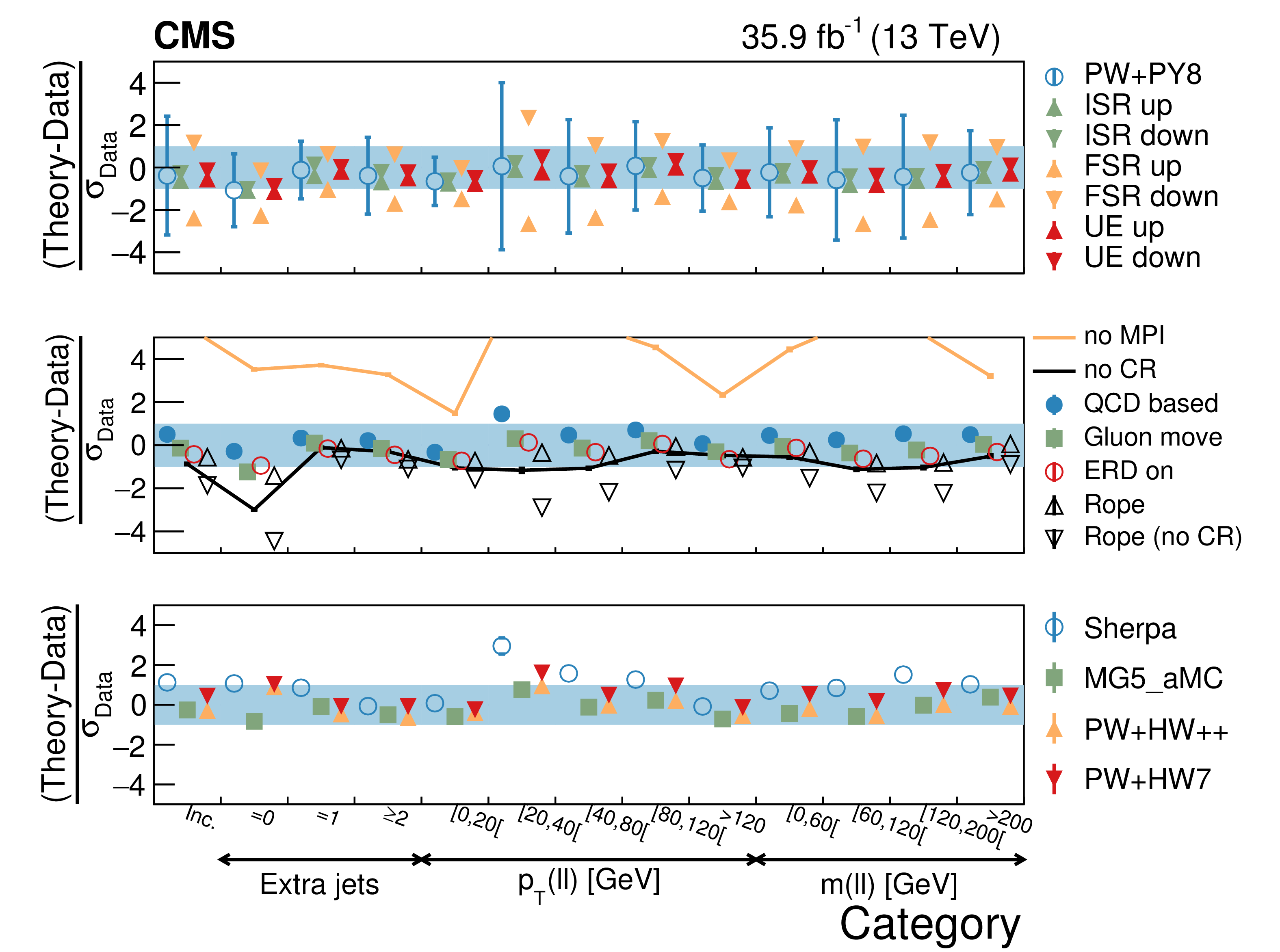
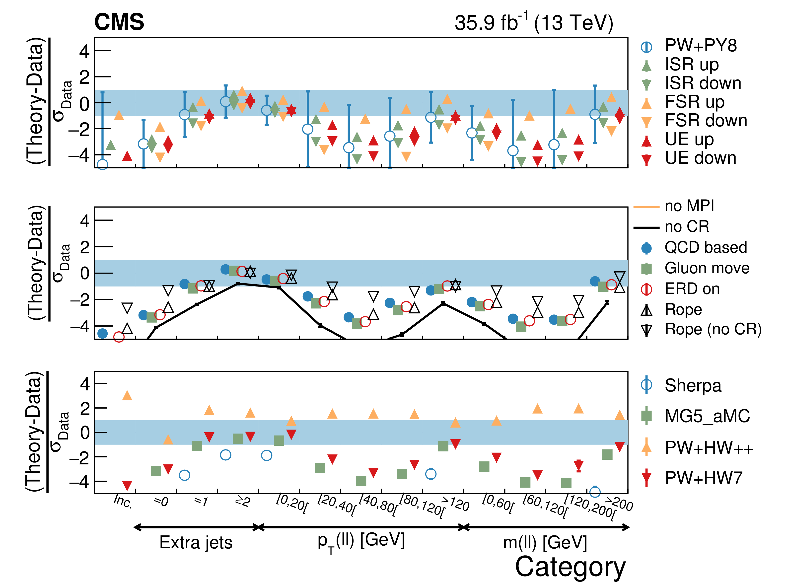
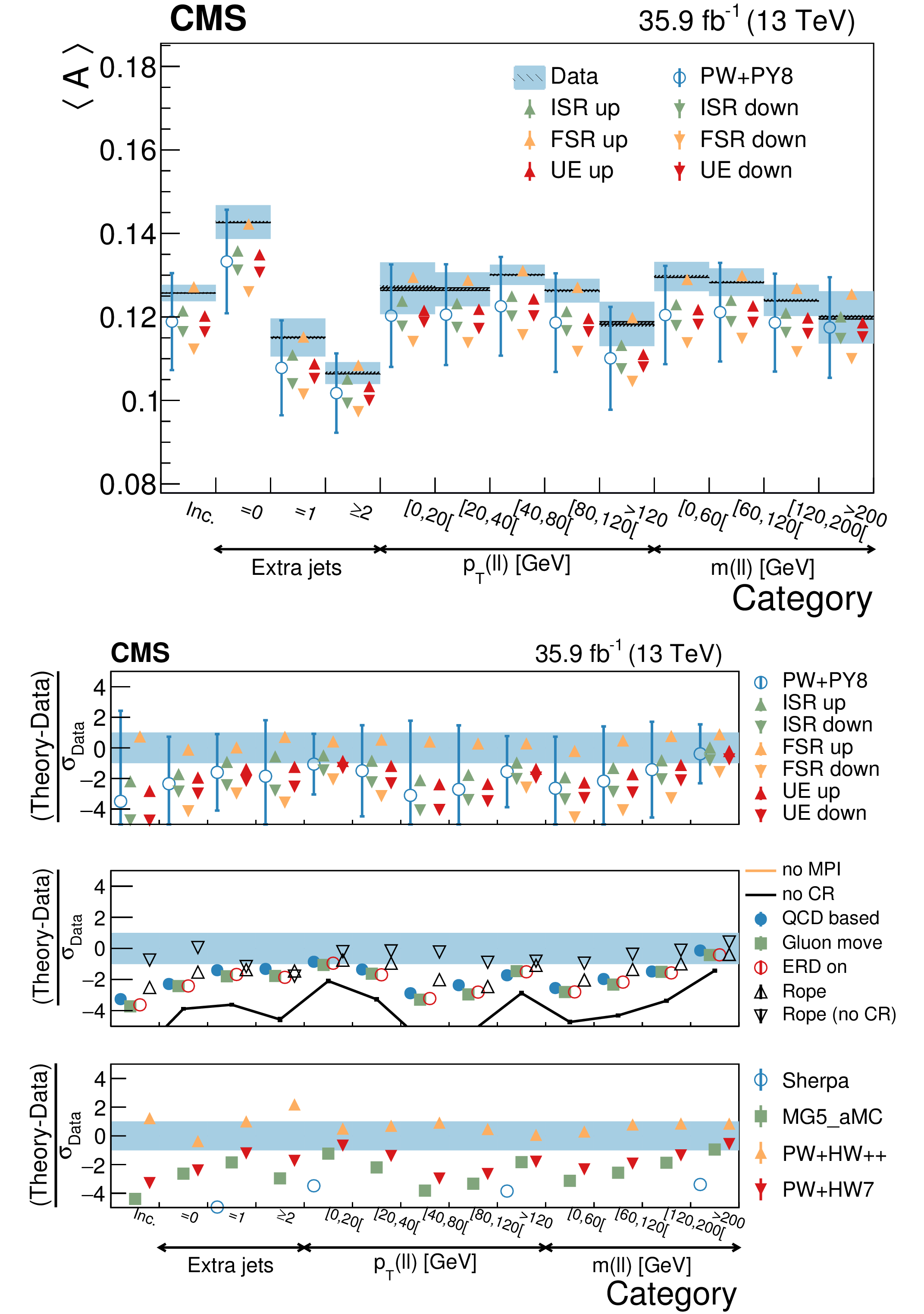
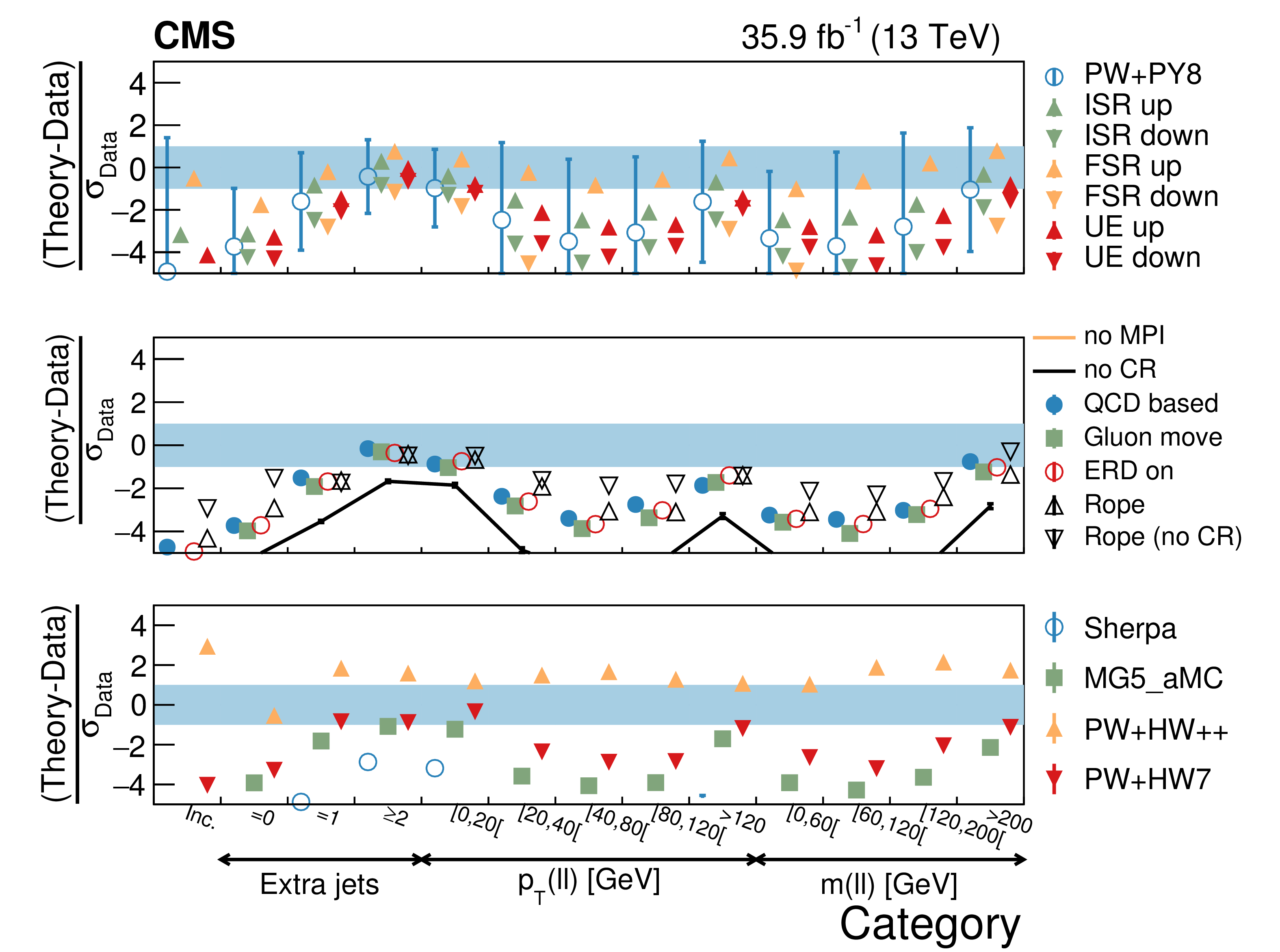
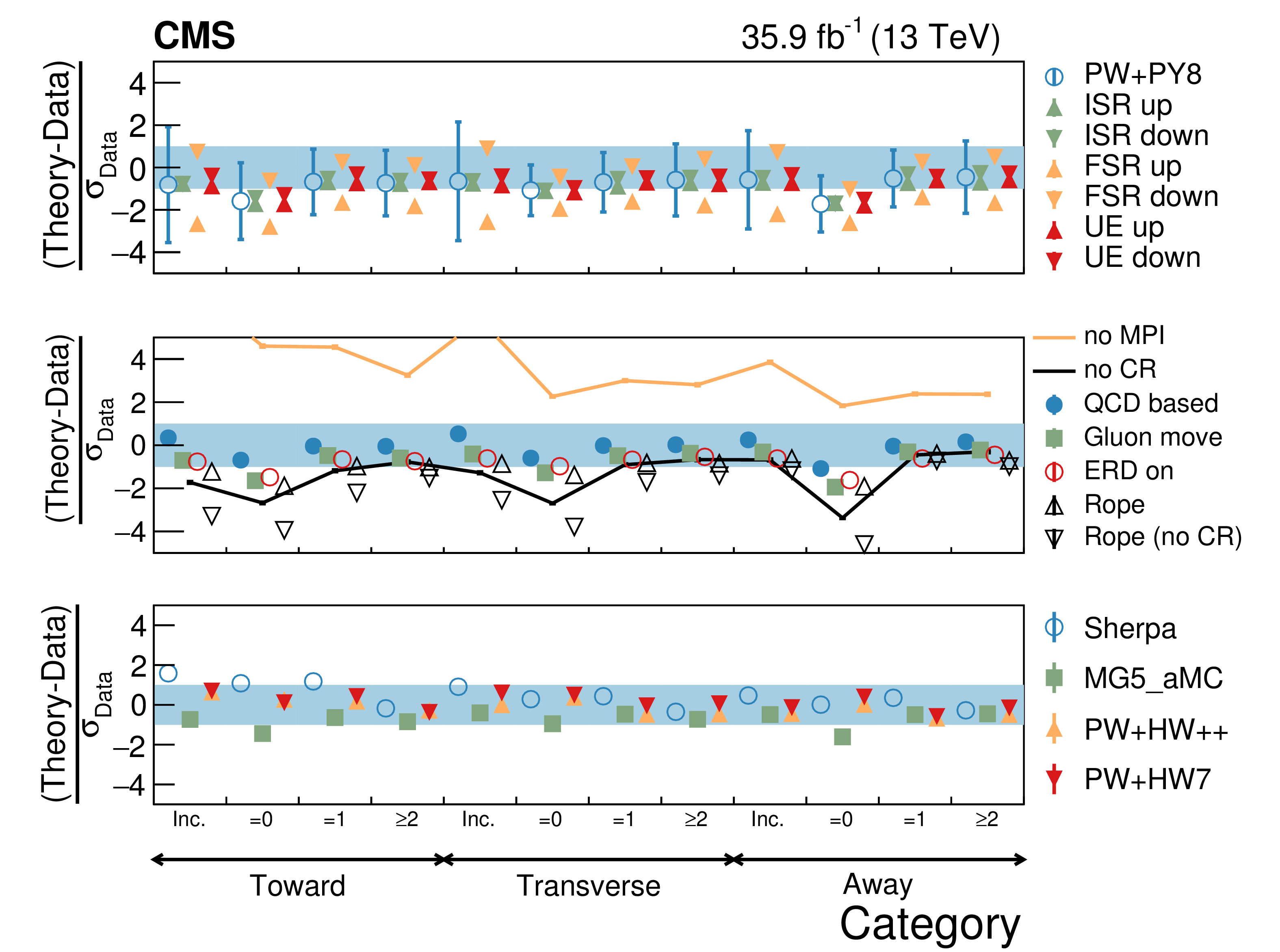
Figure 14:
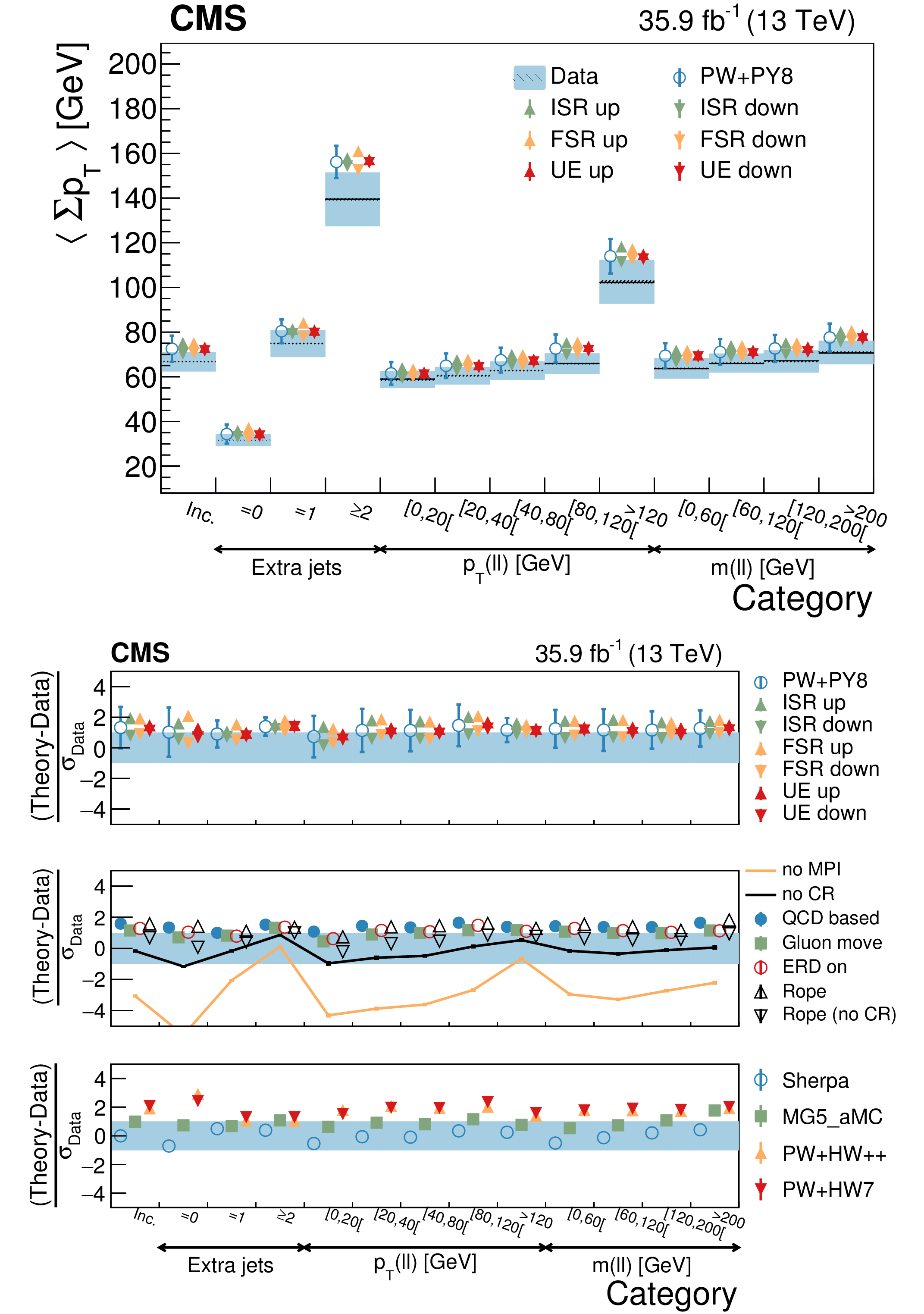
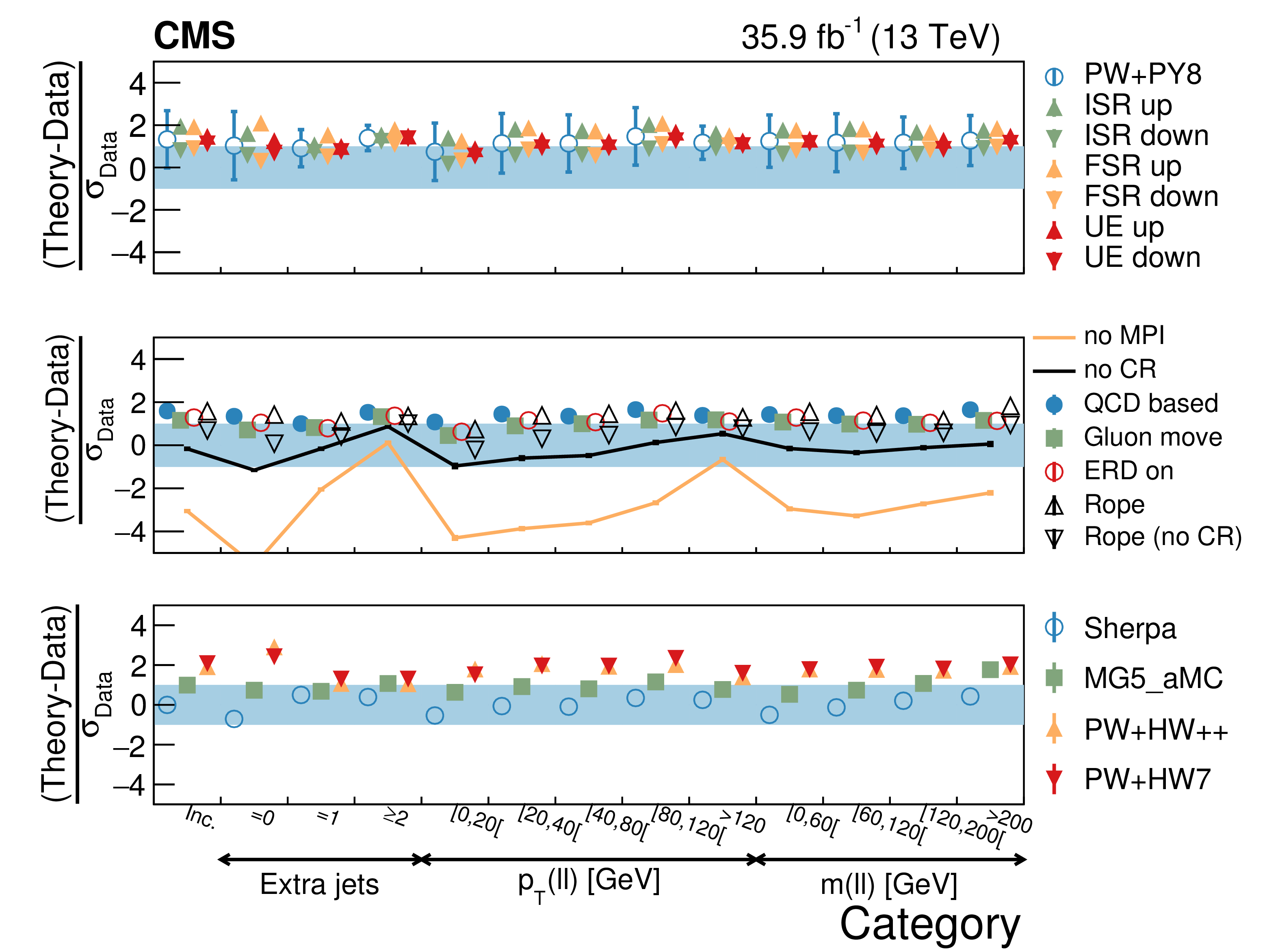
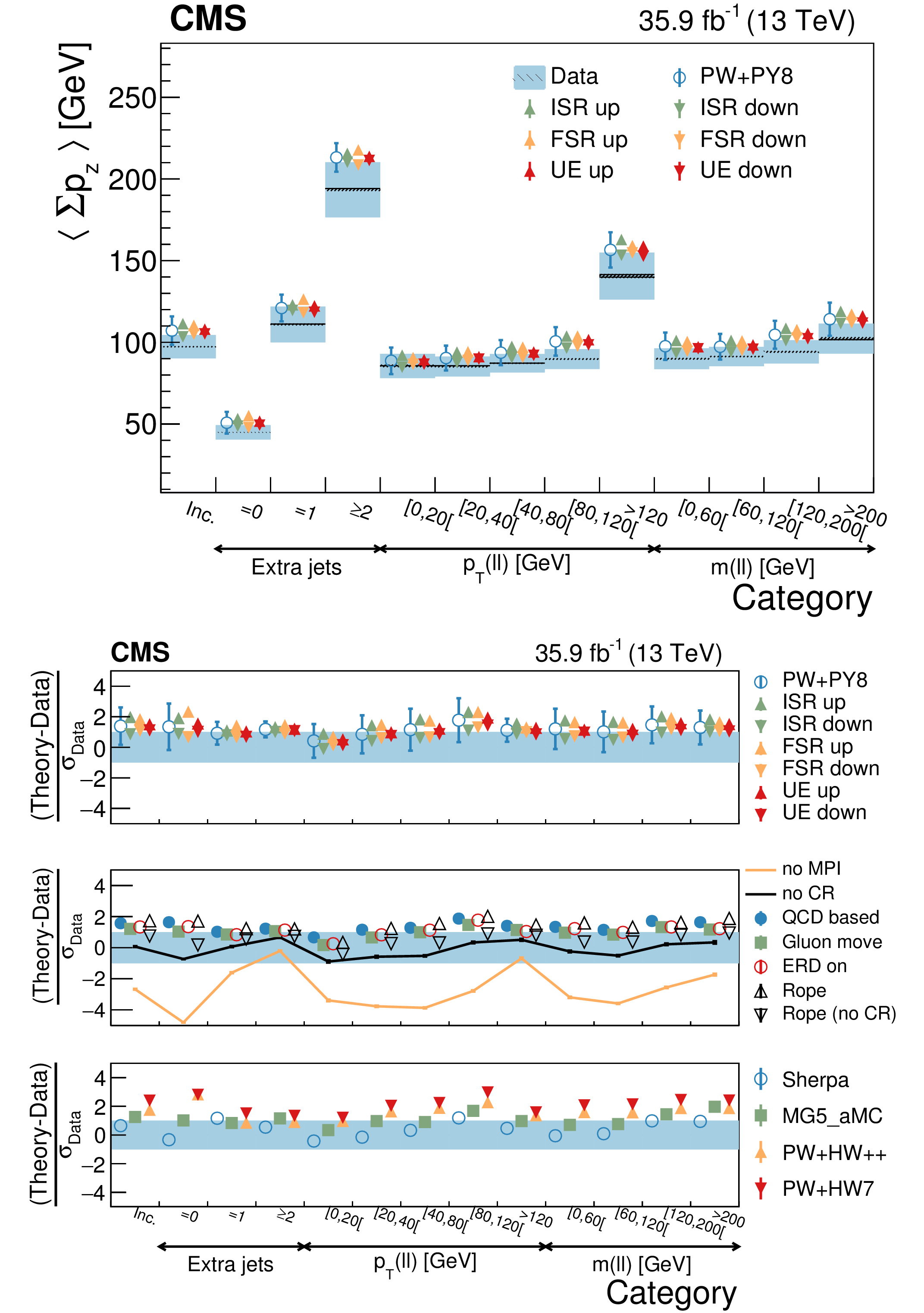
Average $ {N_\text {ch}} $ in different event categories. The mean observed in data (boxes) is compared to the predictions from different models (markers), which are superimposed in the upper figure. The total (statistical) uncertainty of the data is represented by a shaded (hatched) area and the statistical uncertainty of the models is represented with error bars. In the specific case of the POWHEG+PYTHIA8 model the error bars represent the total uncertainty (see text). The lower figure displays the pull between different models and the data, with the different panels corresponding to different sets of models. The bands represent the interval where $ {| \text {pull} |} < $ 1. The error bar for the POWHEG+PYTHIA8 model represents the range of variation of the pull for the different configurations described in the text. |
png pdf |
Figure 14-a:
Average $ {N_\text {ch}} $ in different event categories. The mean observed in data (boxes) is compared to the predictions from different models (markers), which are superimposed in the upper figure. The total (statistical) uncertainty of the data is represented by a shaded (hatched) area and the statistical uncertainty of the models is represented with error bars. In the specific case of the POWHEG+PYTHIA8 model the error bars represent the total uncertainty (see text). The lower figure displays the pull between different models and the data, with the different panels corresponding to different sets of models. The bands represent the interval where $ {| \text {pull} |} < $ 1. The error bar for the POWHEG+PYTHIA8 model represents the range of variation of the pull for the different configurations described in the text. |
png pdf |
Figure 14-b:
Average $ {N_\text {ch}} $ in different event categories. The mean observed in data (boxes) is compared to the predictions from different models (markers), which are superimposed in the upper figure. The total (statistical) uncertainty of the data is represented by a shaded (hatched) area and the statistical uncertainty of the models is represented with error bars. In the specific case of the POWHEG+PYTHIA8 model the error bars represent the total uncertainty (see text). The lower figure displays the pull between different models and the data, with the different panels corresponding to different sets of models. The bands represent the interval where $ {| \text {pull} |} < $ 1. The error bar for the POWHEG+PYTHIA8 model represents the range of variation of the pull for the different configurations described in the text. |
png pdf |
Figure 15:
Average $\Sigma {p_{\mathrm {T}}}$ in different event categories. The conventions of Fig. 14 are used. |

png pdf |
Figure 15-a:
Average $\Sigma {p_{\mathrm {T}}}$ in different event categories. The conventions of Fig. 14 are used. |
png pdf |
Figure 15-b:
Average $\Sigma {p_{\mathrm {T}}}$ in different event categories. The conventions of Fig. 14 are used. |
png pdf |
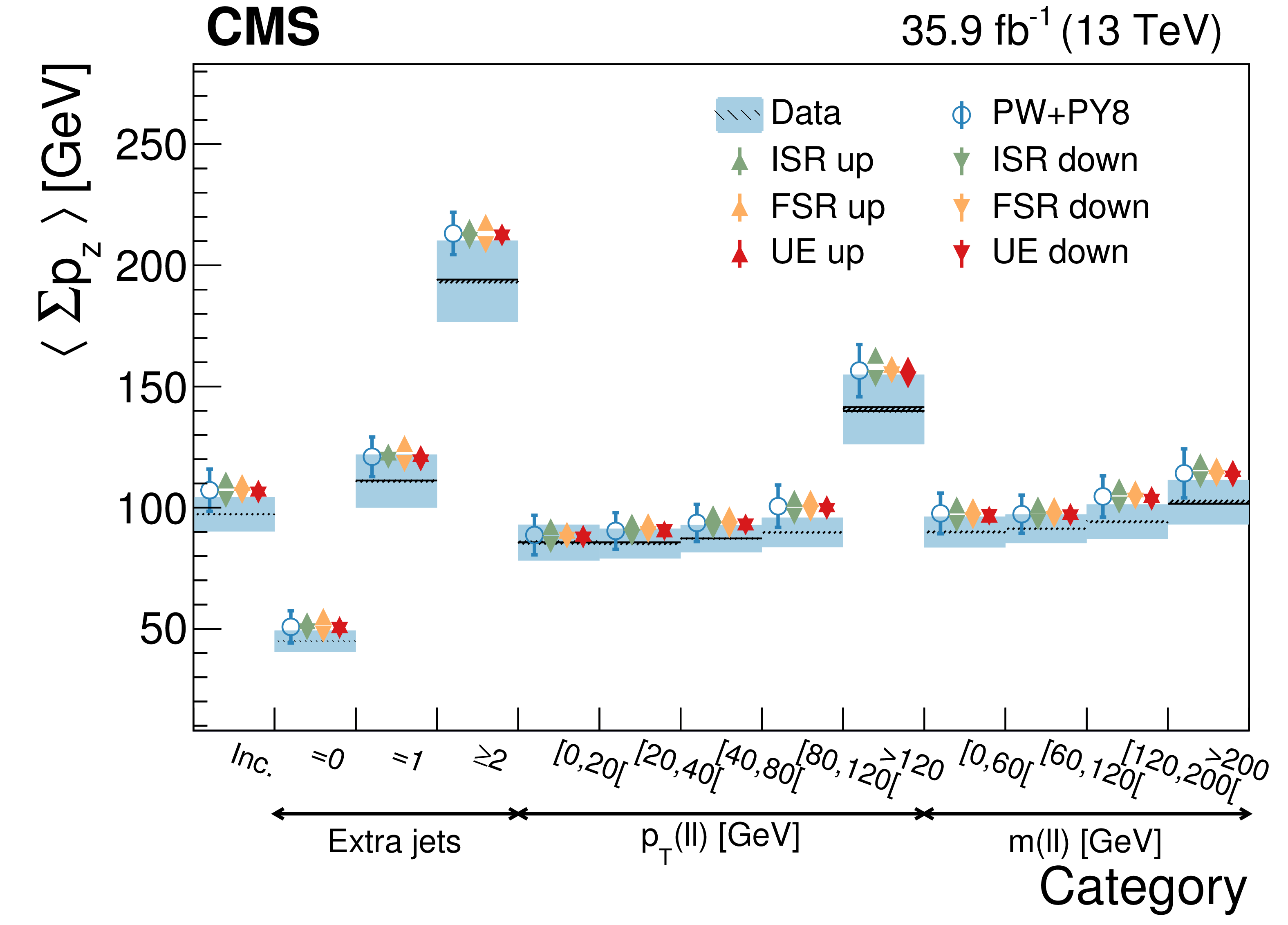
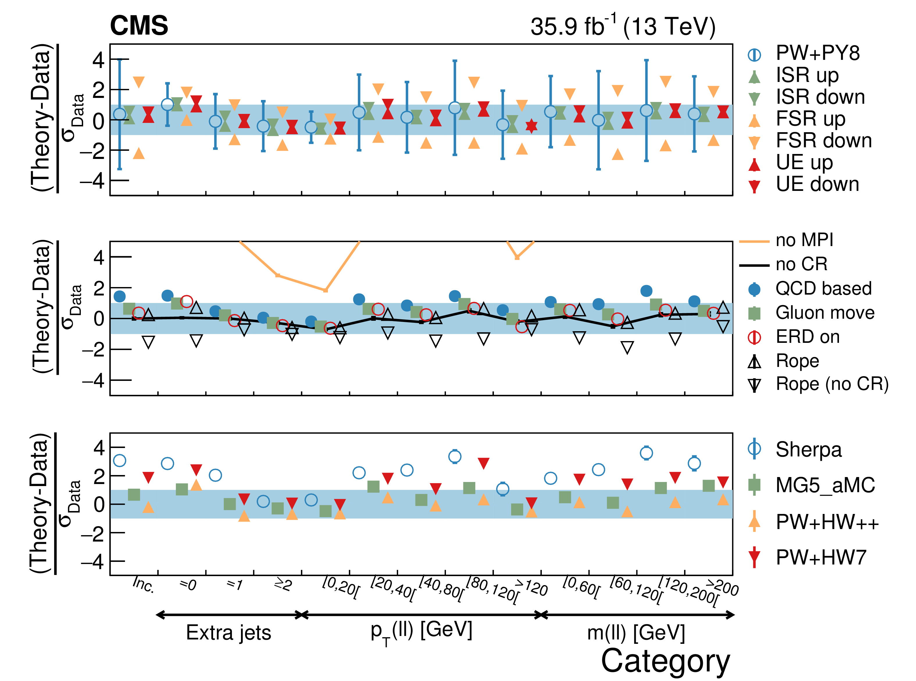
Figure 16:
Average ${\Sigma p_{z}}$ in different categories. The conventions of Fig. 14 are used. |
png pdf |
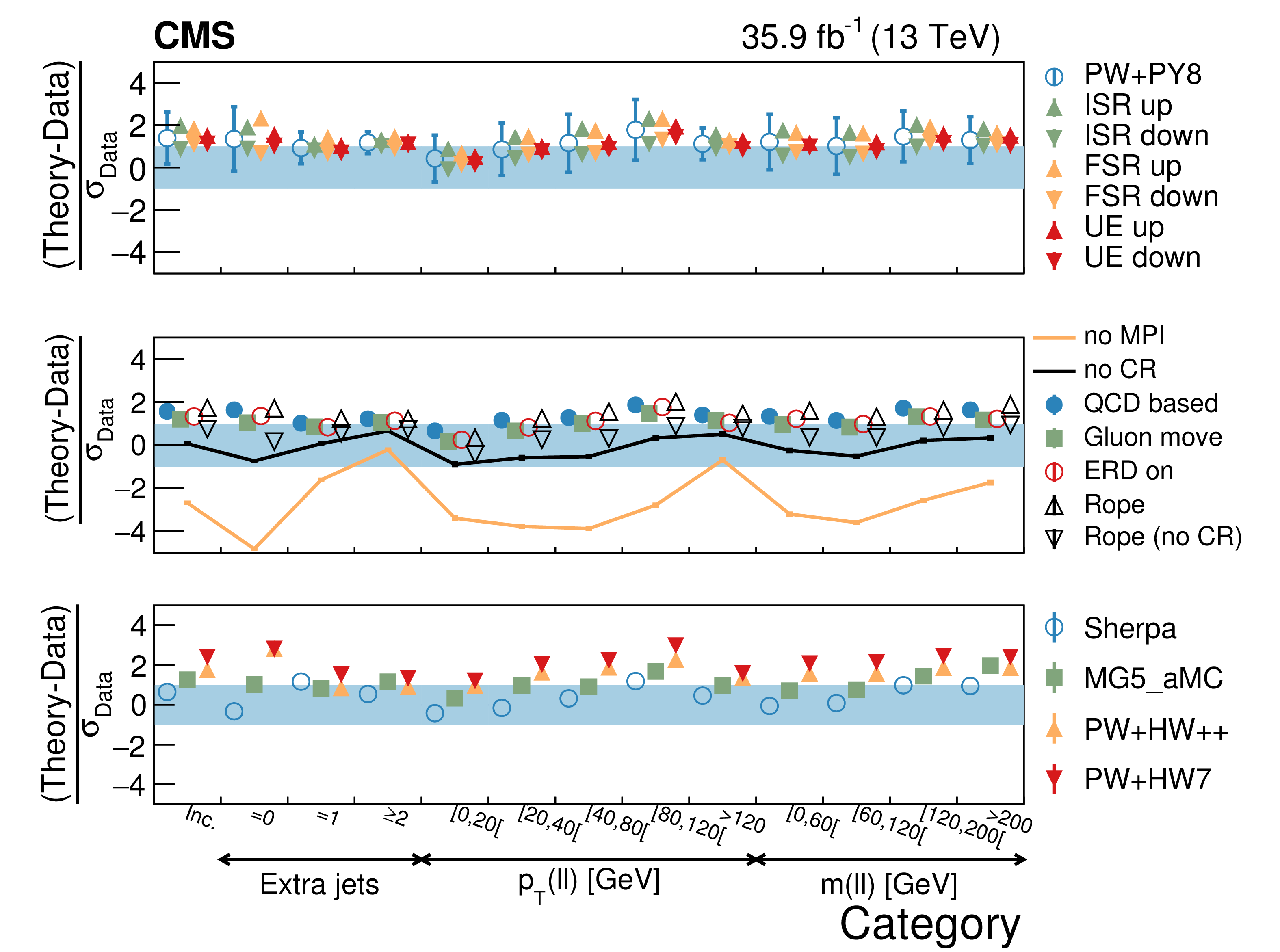
Figure 16-a:
Average ${\Sigma p_{z}}$ in different categories. The conventions of Fig. 14 are used. |
png pdf |
Figure 16-b:
Average ${\Sigma p_{z}}$ in different categories. The conventions of Fig. 14 are used. |
png pdf |
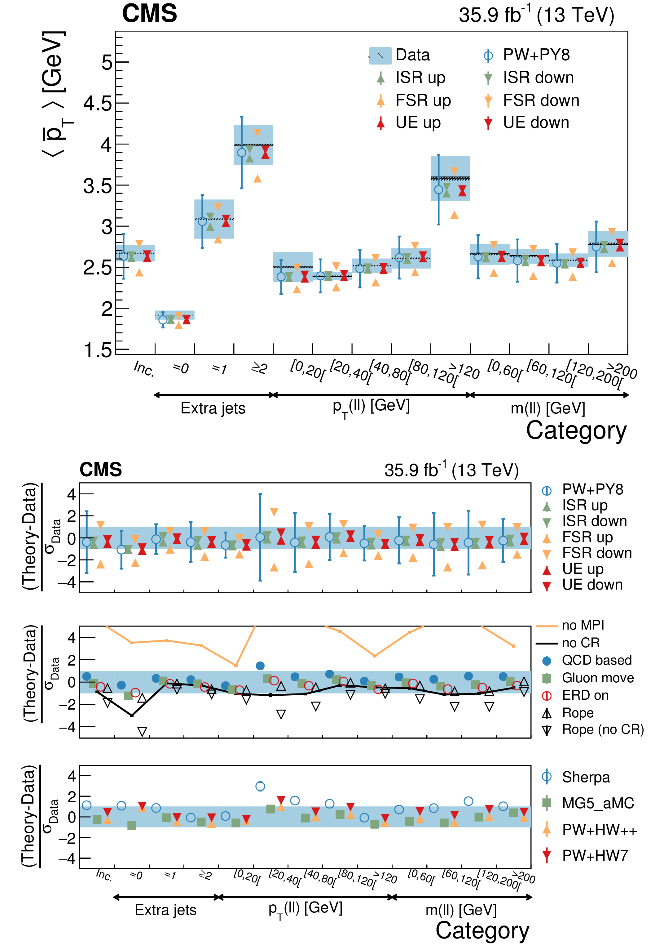
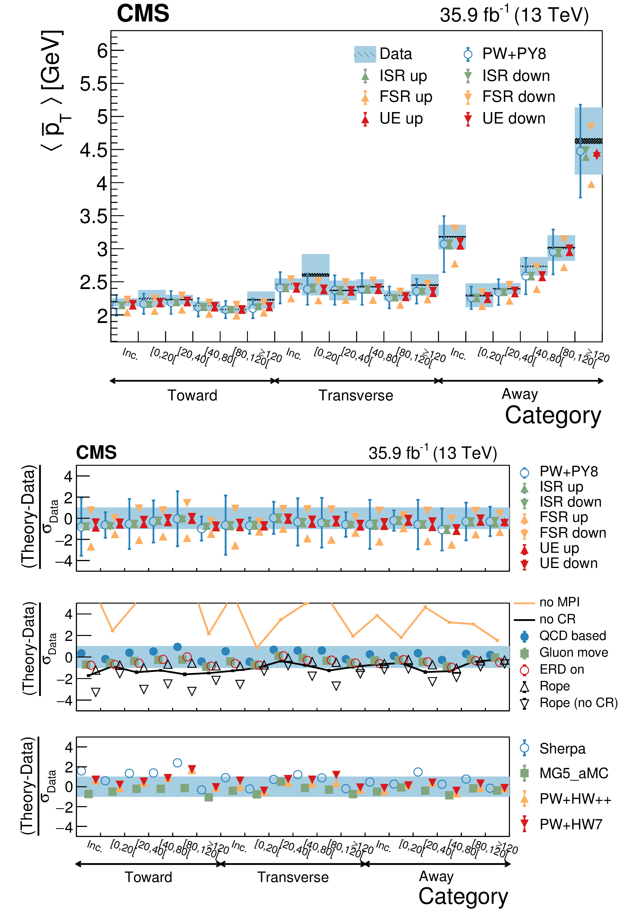
Figure 17:
Average ${{\overline {{p_{\mathrm {T}}}}}}$ in different categories. The conventions of Fig. 14 are used. |
png pdf |
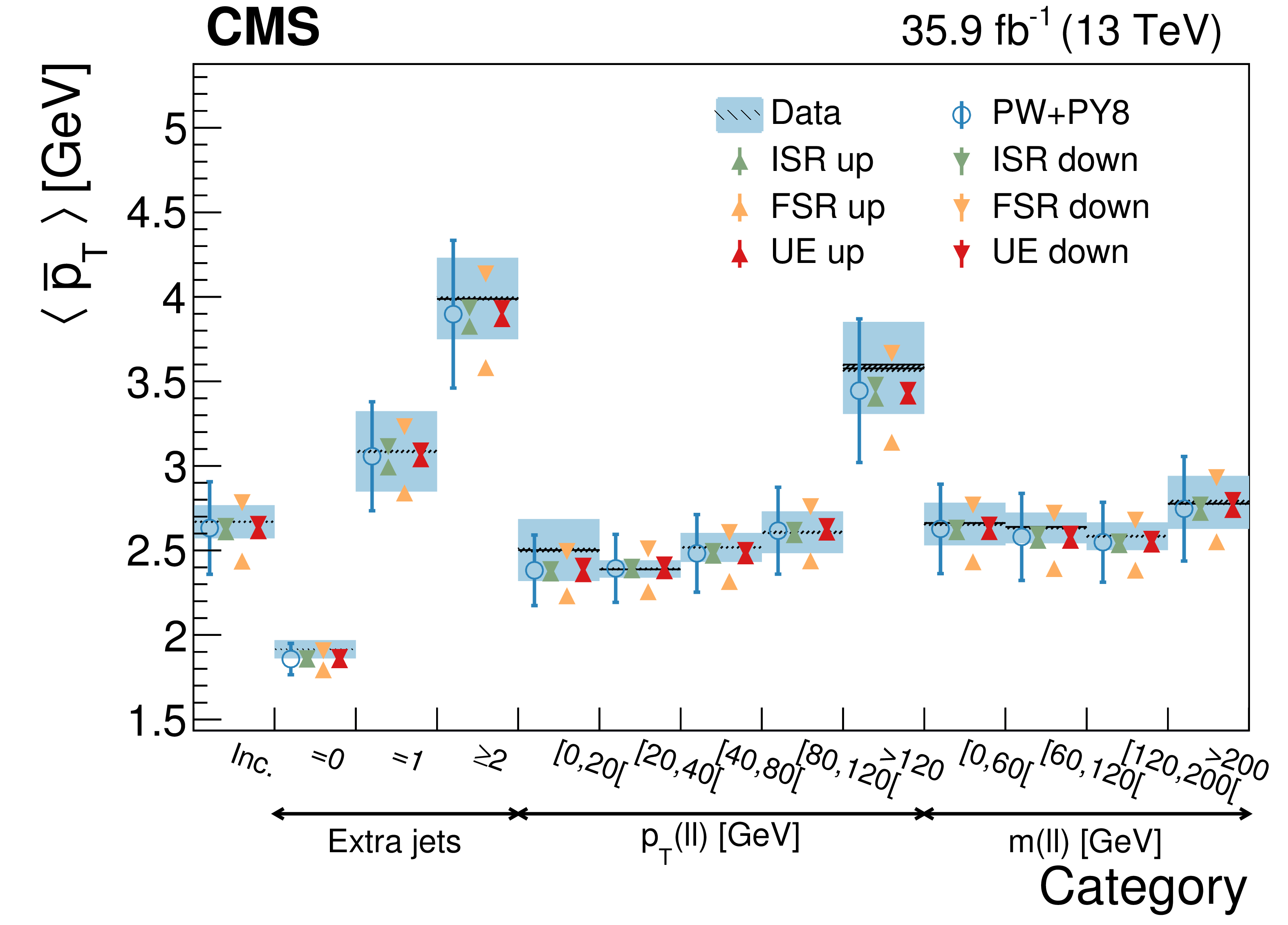
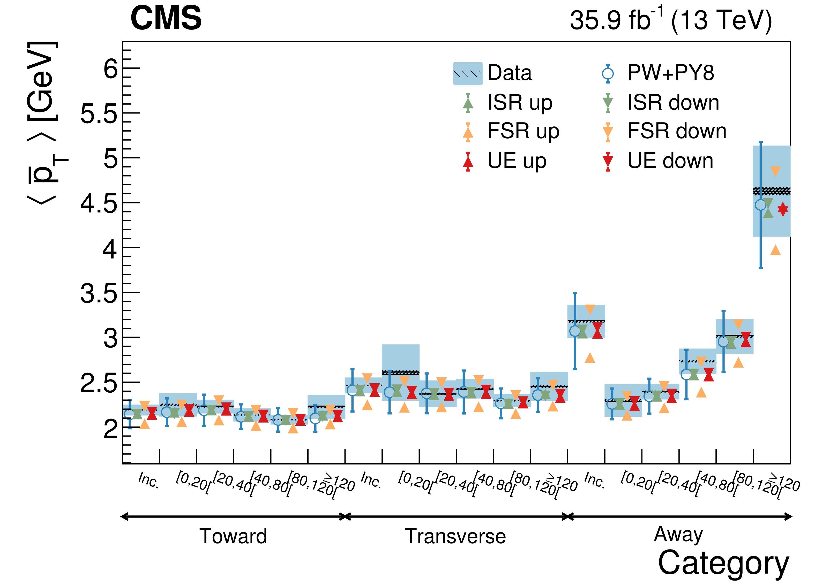
Figure 17-a:
Average ${{\overline {{p_{\mathrm {T}}}}}}$ in different categories. The conventions of Fig. 14 are used. |
png pdf |
Figure 17-b:
Average ${{\overline {{p_{\mathrm {T}}}}}}$ in different categories. The conventions of Fig. 14 are used. |

png pdf |
Figure 18:
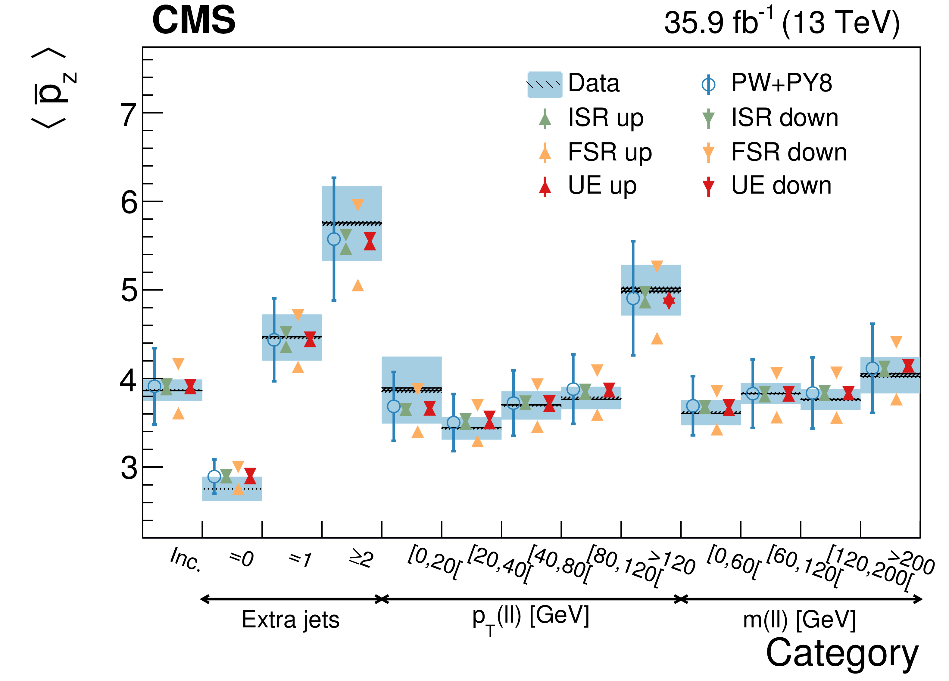
Average ${{\overline {p_z}}}$ in different categories. The conventions of Fig. 14 are used. |
png pdf |
Figure 18-a:
Average ${{\overline {p_z}}}$ in different categories. The conventions of Fig. 14 are used. |
png pdf |
Figure 18-b:
Average ${{\overline {p_z}}}$ in different categories. The conventions of Fig. 14 are used. |
png pdf |
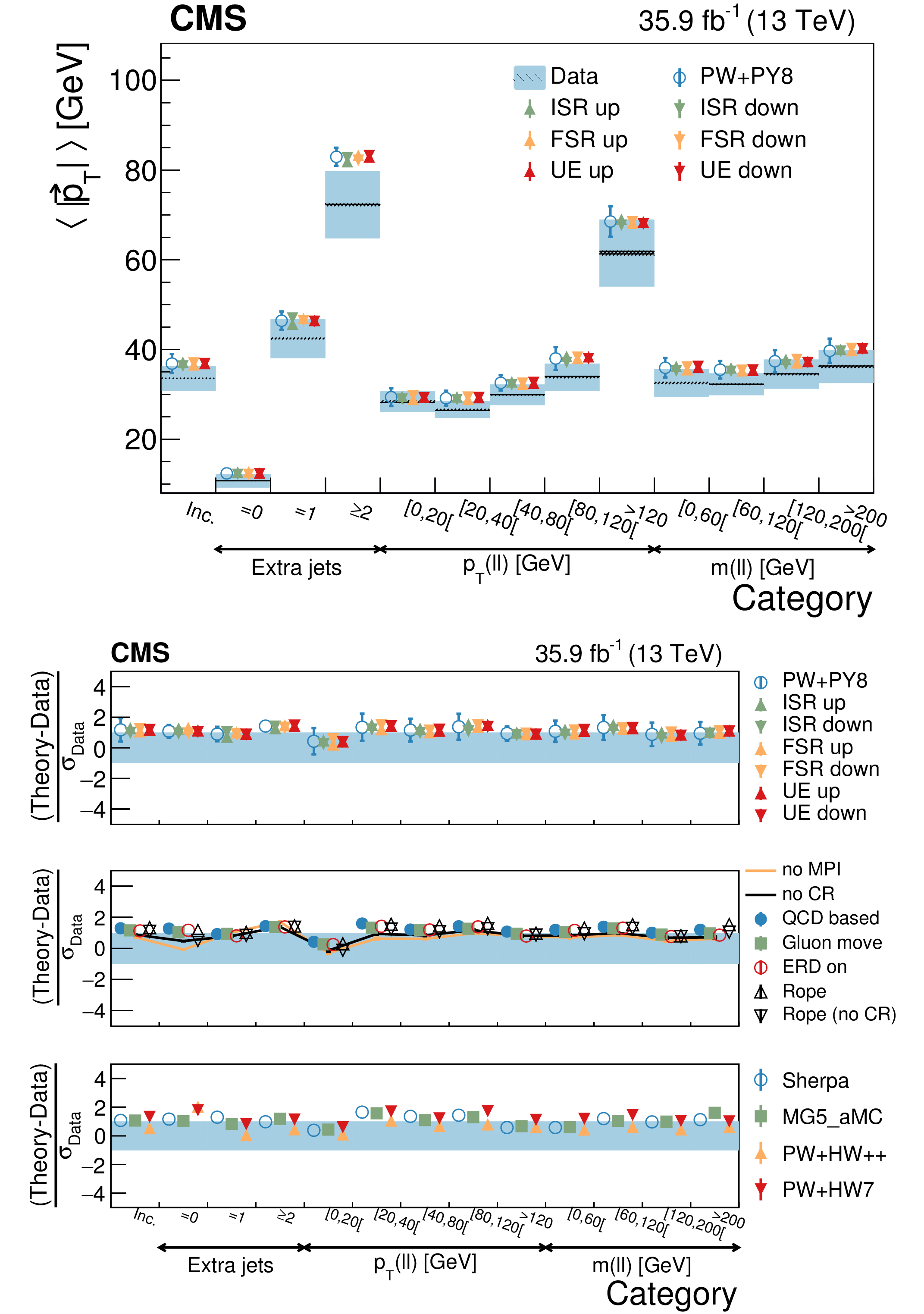
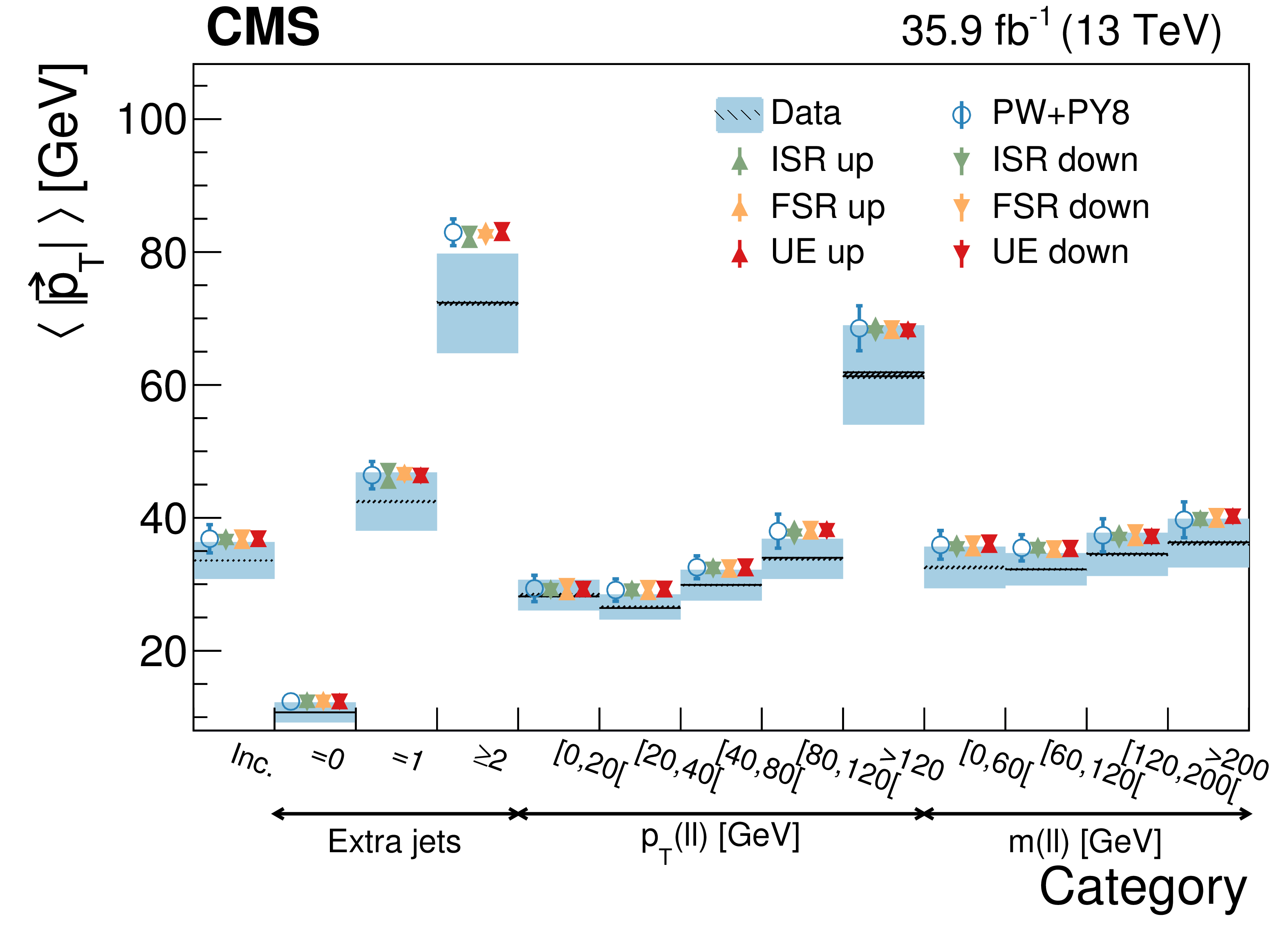
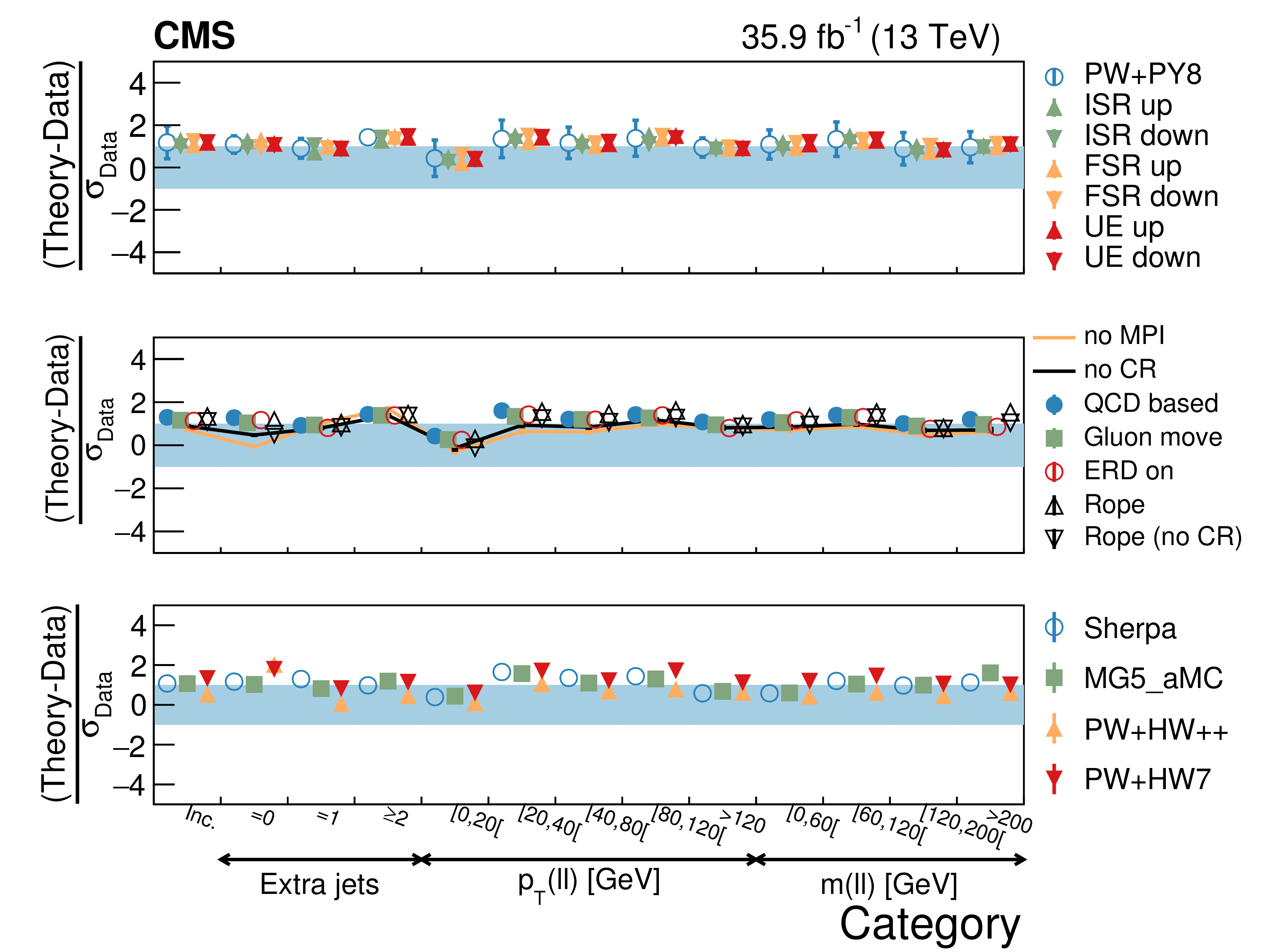
Figure 19:
Average $ {{| {\vec{p}_{\mathrm {T}}} |}} $ in different categories. The conventions of Fig. 14 are used. |
png pdf |
Figure 19-a:
Average $ {{| {\vec{p}_{\mathrm {T}}} |}} $ in different categories. The conventions of Fig. 14 are used. |
png pdf |
Figure 19-b:
Average $ {{| {\vec{p}_{\mathrm {T}}} |}} $ in different categories. The conventions of Fig. 14 are used. |
png pdf |
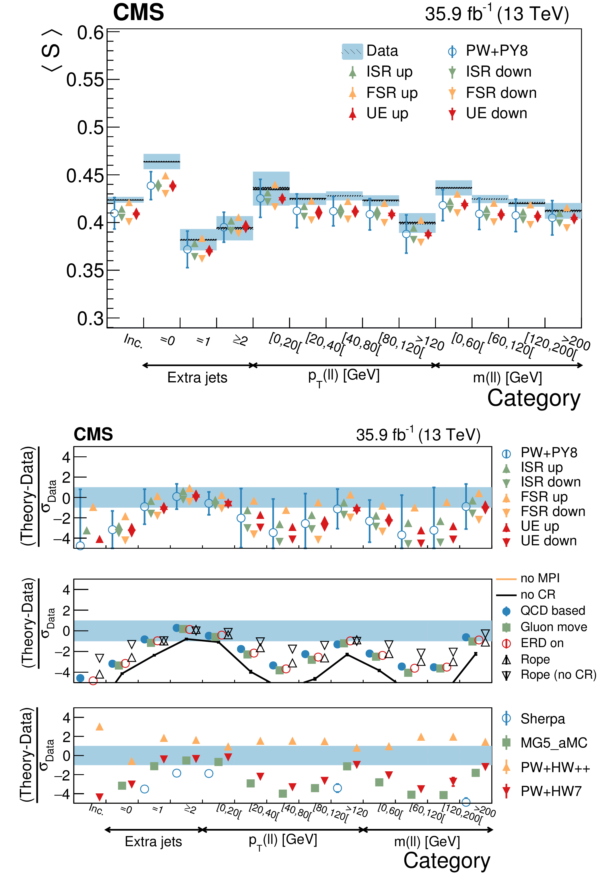
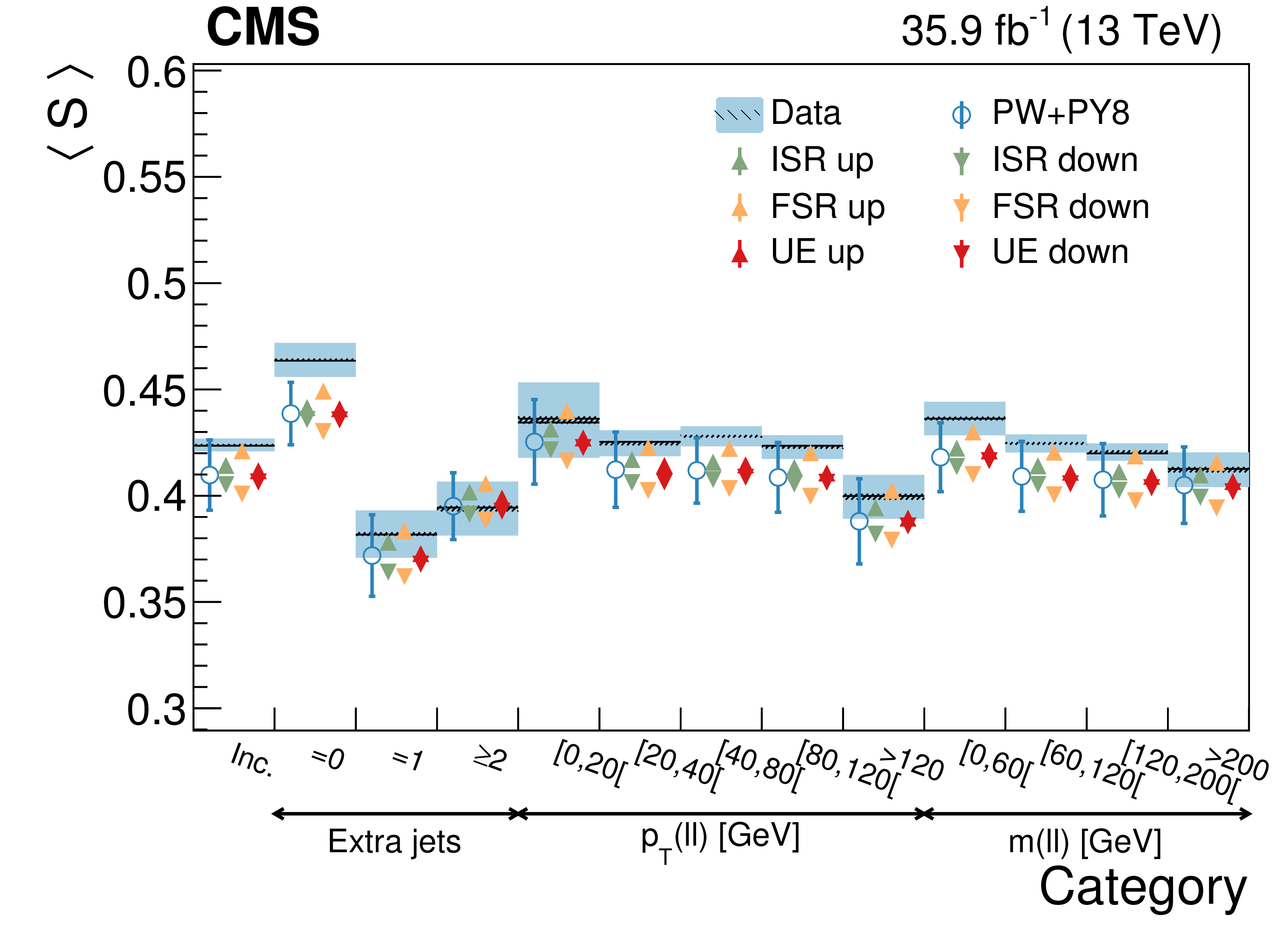
Figure 20:
Average sphericity in different categories. The conventions of Fig. 14 are used. |
png pdf |
Figure 20-a:
Average sphericity in different categories. The conventions of Fig. 14 are used. |
png pdf |
Figure 20-b:
Average sphericity in different categories. The conventions of Fig. 14 are used. |
png pdf |
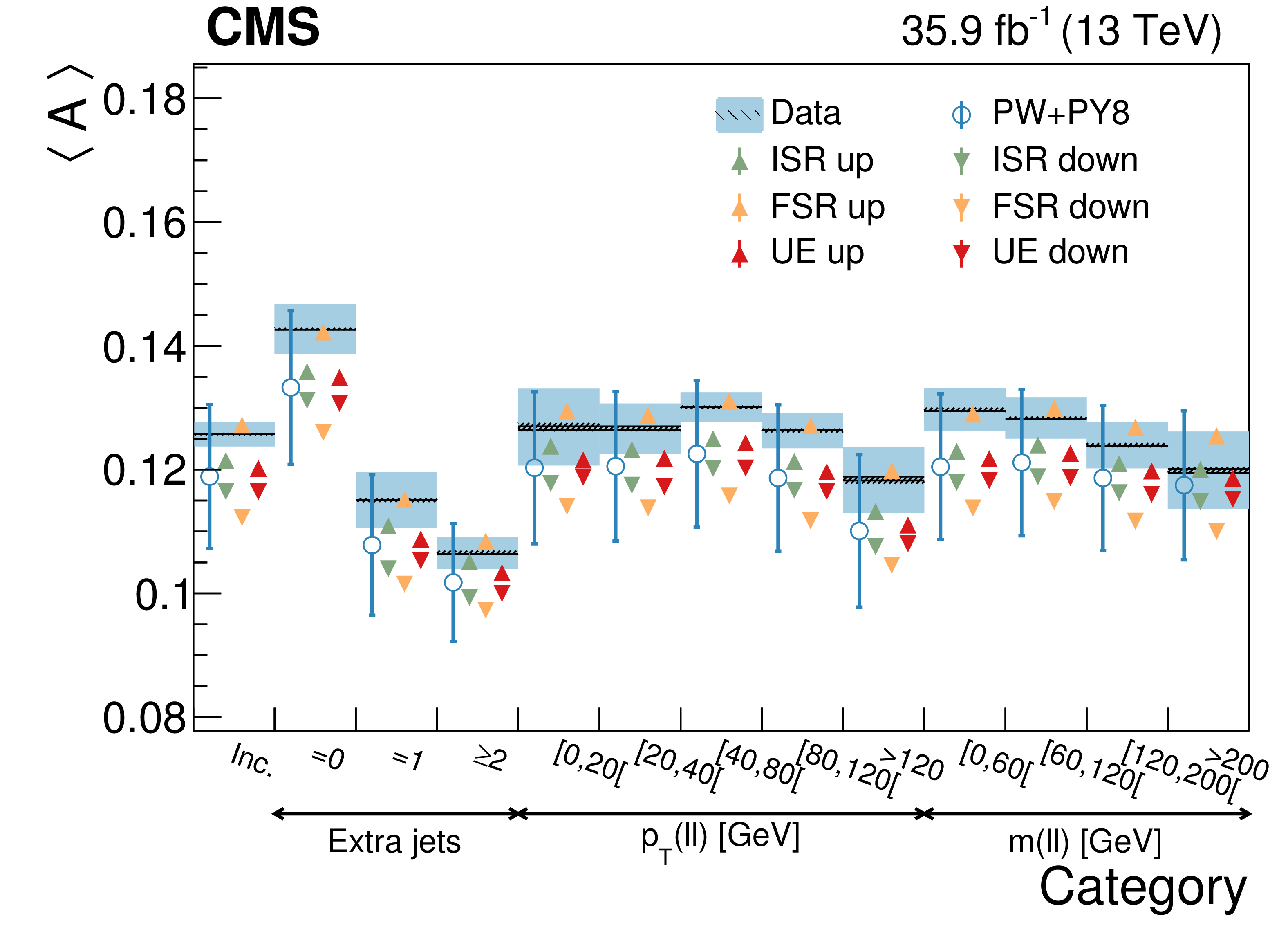
Figure 21:
Average aplanarity in different categories. The conventions of Fig. 14 are used. |
png pdf |
Figure 21-a:
Average aplanarity in different categories. The conventions of Fig. 14 are used. |

png pdf |
Figure 21-b:
Average aplanarity in different categories. The conventions of Fig. 14 are used. |

png pdf |
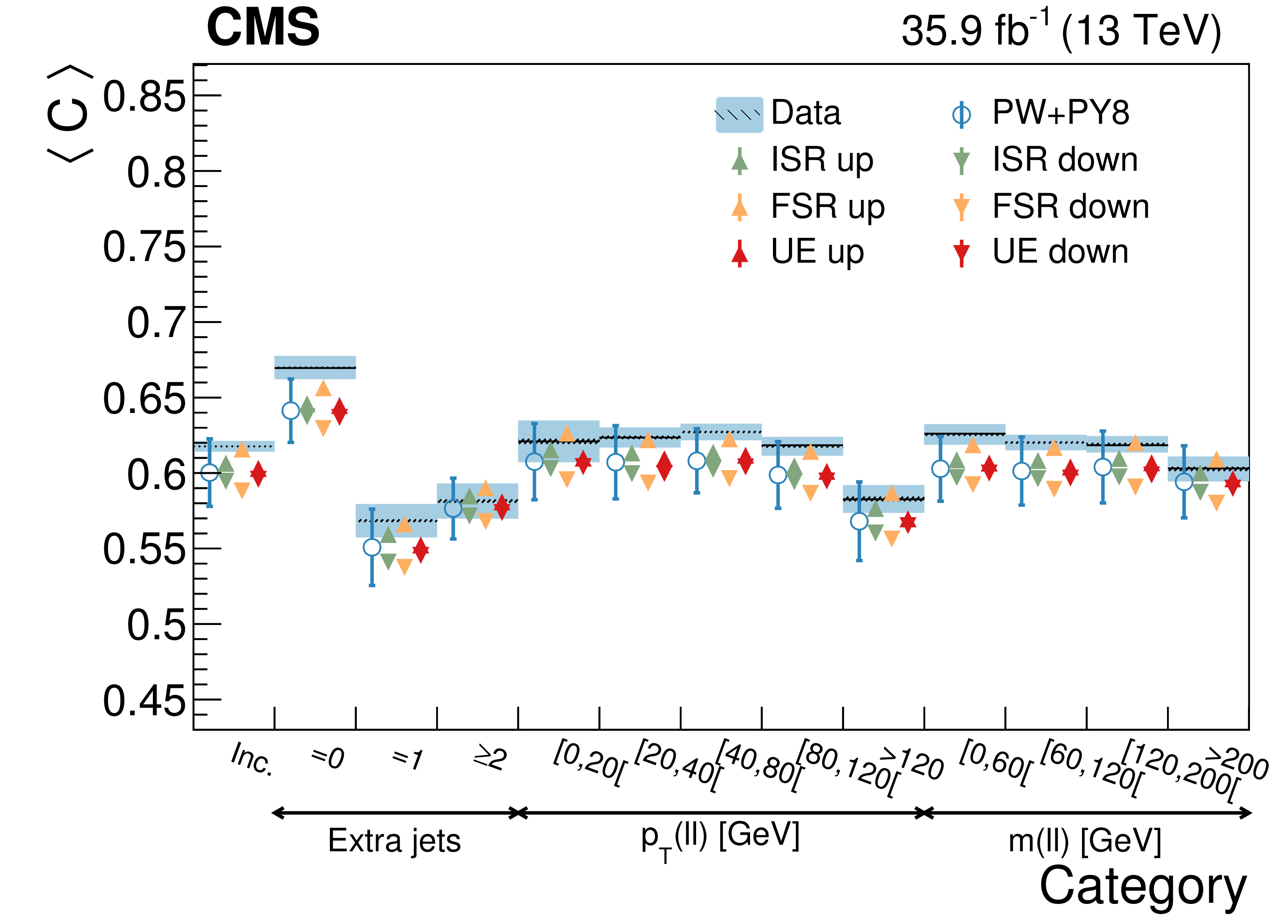
Figure 22:
Average $C$ in different categories. The conventions of Fig. 14 are used. |
png pdf |
Figure 22-a:
Average $C$ in different categories. The conventions of Fig. 14 are used. |
png pdf |
Figure 22-b:
Average $C$ in different categories. The conventions of Fig. 14 are used. |
png pdf |
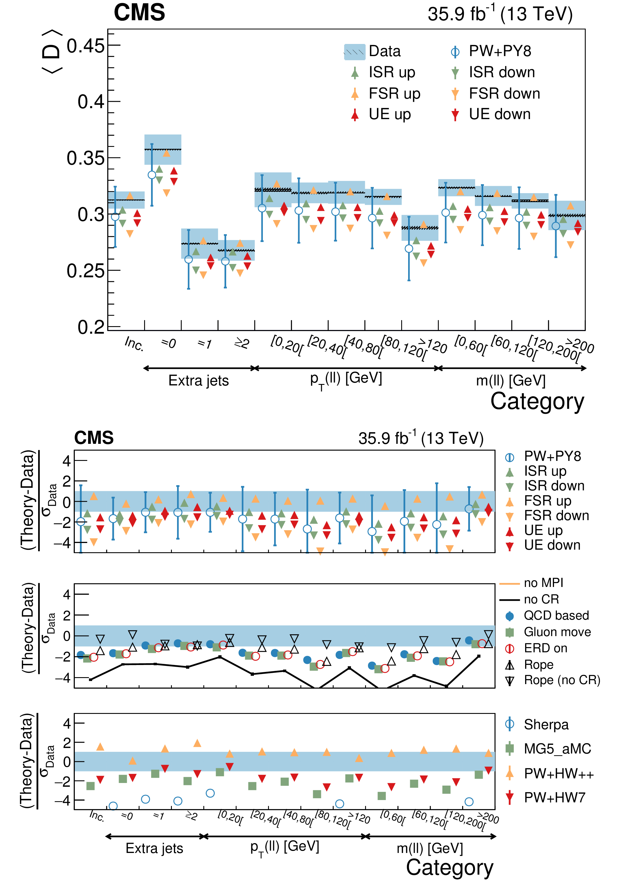
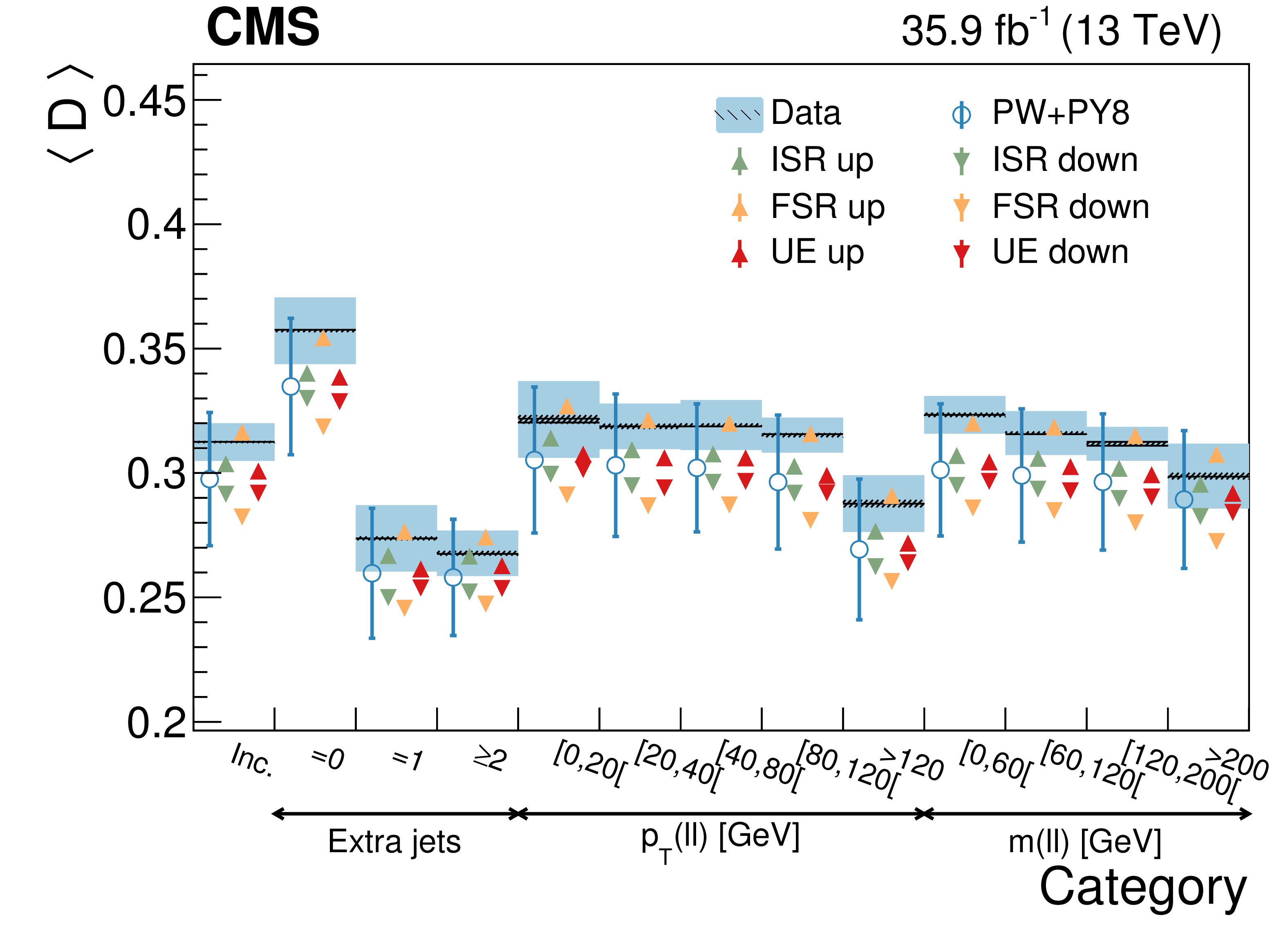
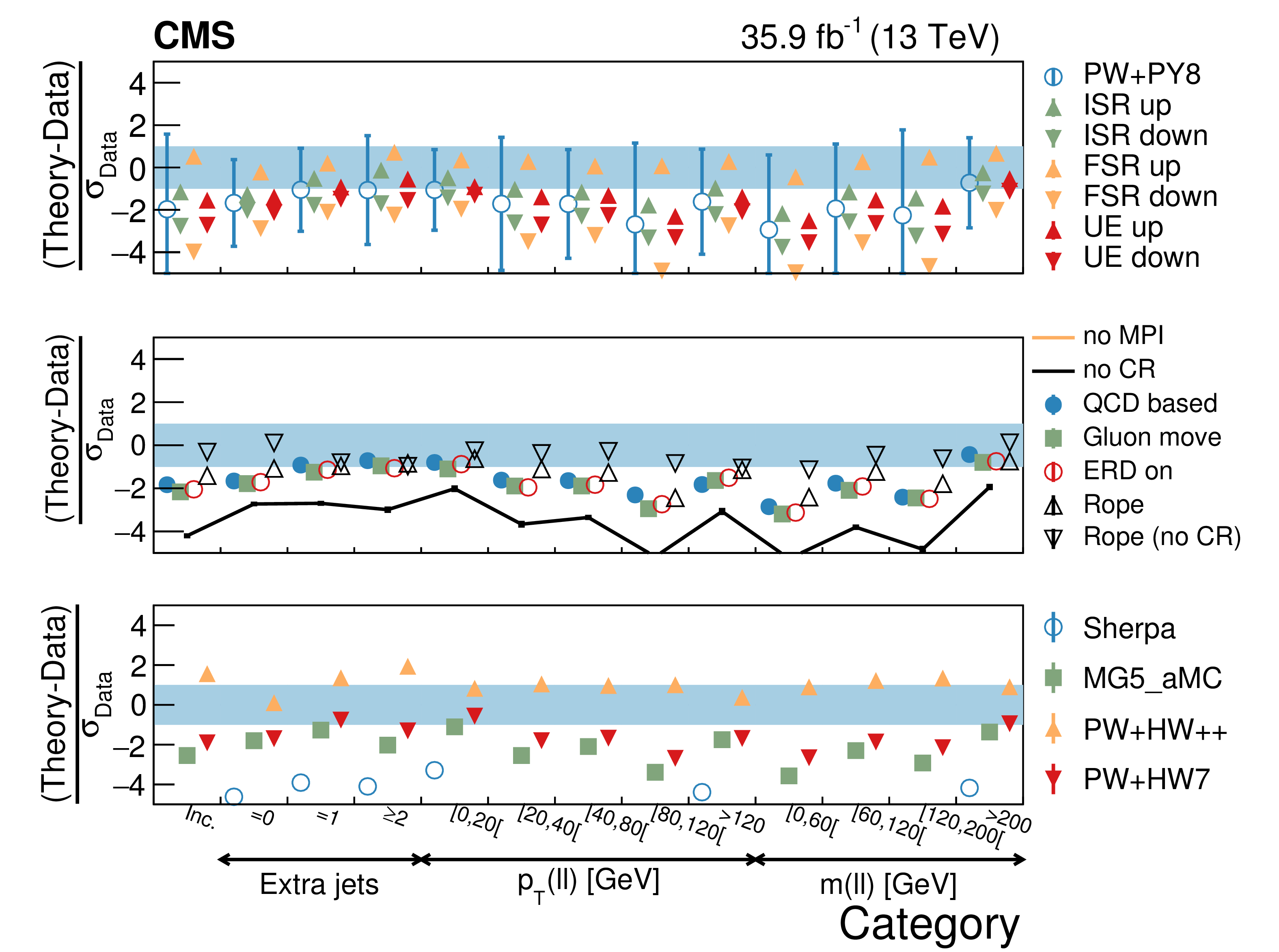
Figure 23:
Average $D$ in different categories. The conventions of Fig. 14 are used. |
png pdf |
Figure 23-a:
Average $D$ in different categories. The conventions of Fig. 14 are used. |
png pdf |
Figure 23-b:
Average $D$ in different categories. The conventions of Fig. 14 are used. |
png pdf |
Figure 24:
Average ${{\overline {{p_{\mathrm {T}}}}}}$ in different $ {{p_{\mathrm {T}}} (\ell \ell)} $ categories. The conventions of Fig. 14 are used. |
png pdf |
Figure 24-a:
Average ${{\overline {{p_{\mathrm {T}}}}}}$ in different $ {{p_{\mathrm {T}}} (\ell \ell)} $ categories. The conventions of Fig. 14 are used. |

png pdf |
Figure 24-b:
Average ${{\overline {{p_{\mathrm {T}}}}}}$ in different $ {{p_{\mathrm {T}}} (\ell \ell)} $ categories. The conventions of Fig. 14 are used. |
png pdf |
Figure 25:
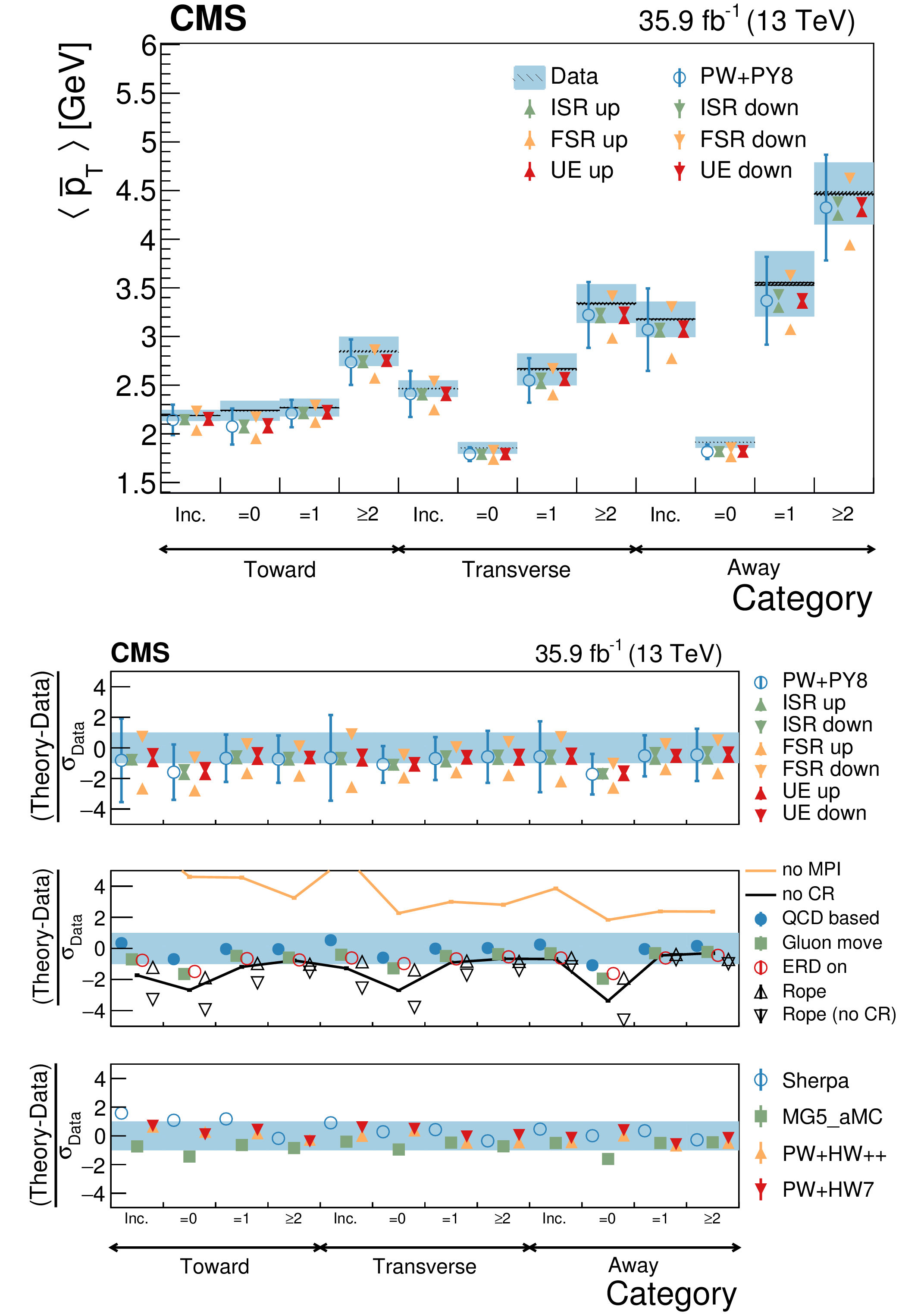
Average ${{\overline {{p_{\mathrm {T}}}}}}$ in different jet multiplicity categories. The conventions of Fig. 14 are used. |
png pdf |
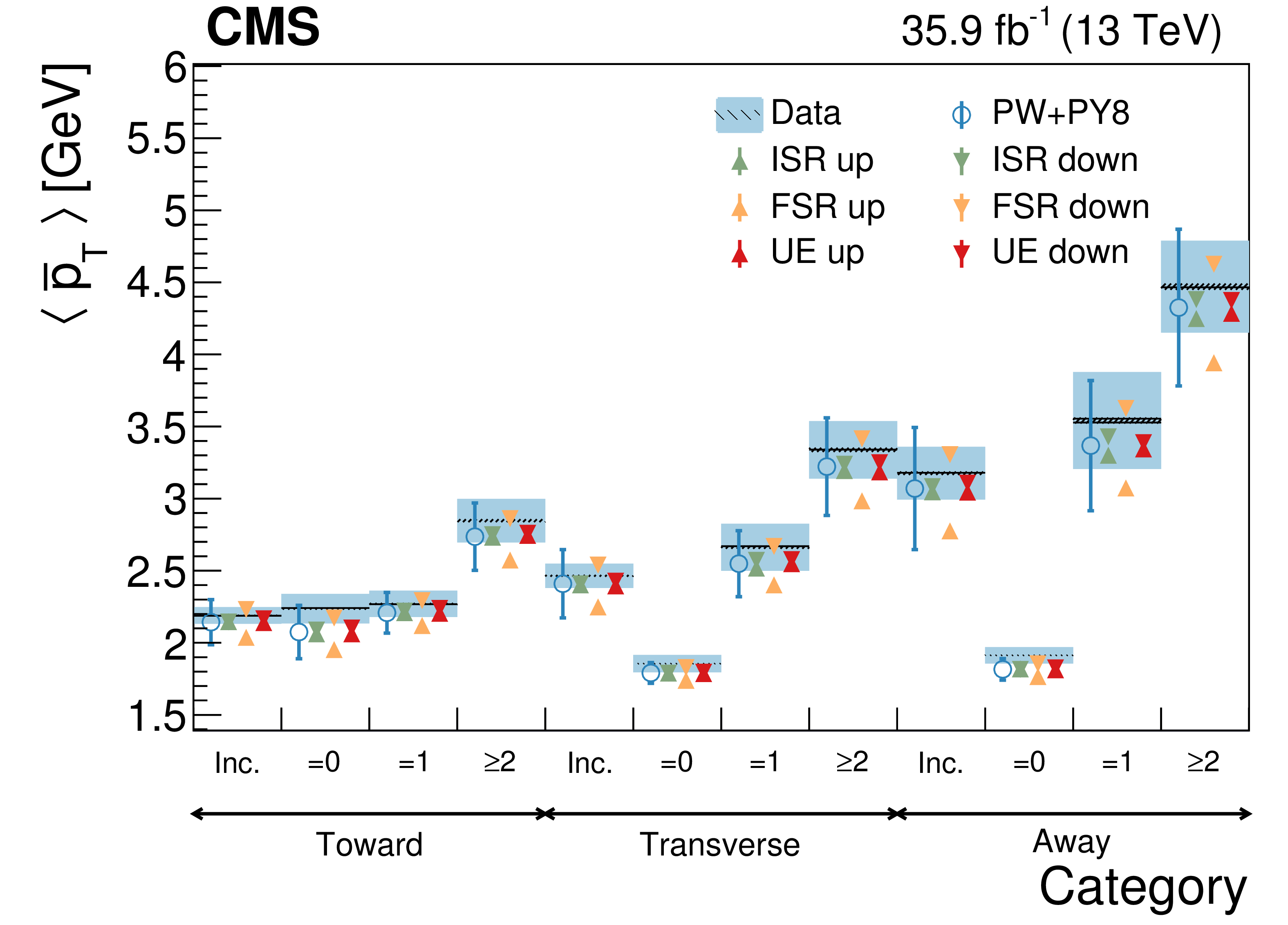
Figure 25-a:
Average ${{\overline {{p_{\mathrm {T}}}}}}$ in different jet multiplicity categories. The conventions of Fig. 14 are used. |
png pdf |
Figure 25-b:
Average ${{\overline {{p_{\mathrm {T}}}}}}$ in different jet multiplicity categories. The conventions of Fig. 14 are used. |

png pdf |
Figure 26:
Scan of the $\chi ^2$ as a function of the value of $ {\alpha _S} ^\text {FSR}(M_ {\mathrm {Z}})$ employed in the POWHEG+PYTHIA8 simulation, when the inclusive ${{\overline {{p_{\mathrm {T}}}}}}$ or the ${{\overline {{p_{\mathrm {T}}}}}}$ distribution measured in different regions is used. The curves result from a fourth-order polynomial interpolation between the simulated $ {\alpha _S} ^\text {FSR}(M_ {\mathrm {Z}})$ points. |
| Tables | |
png pdf |
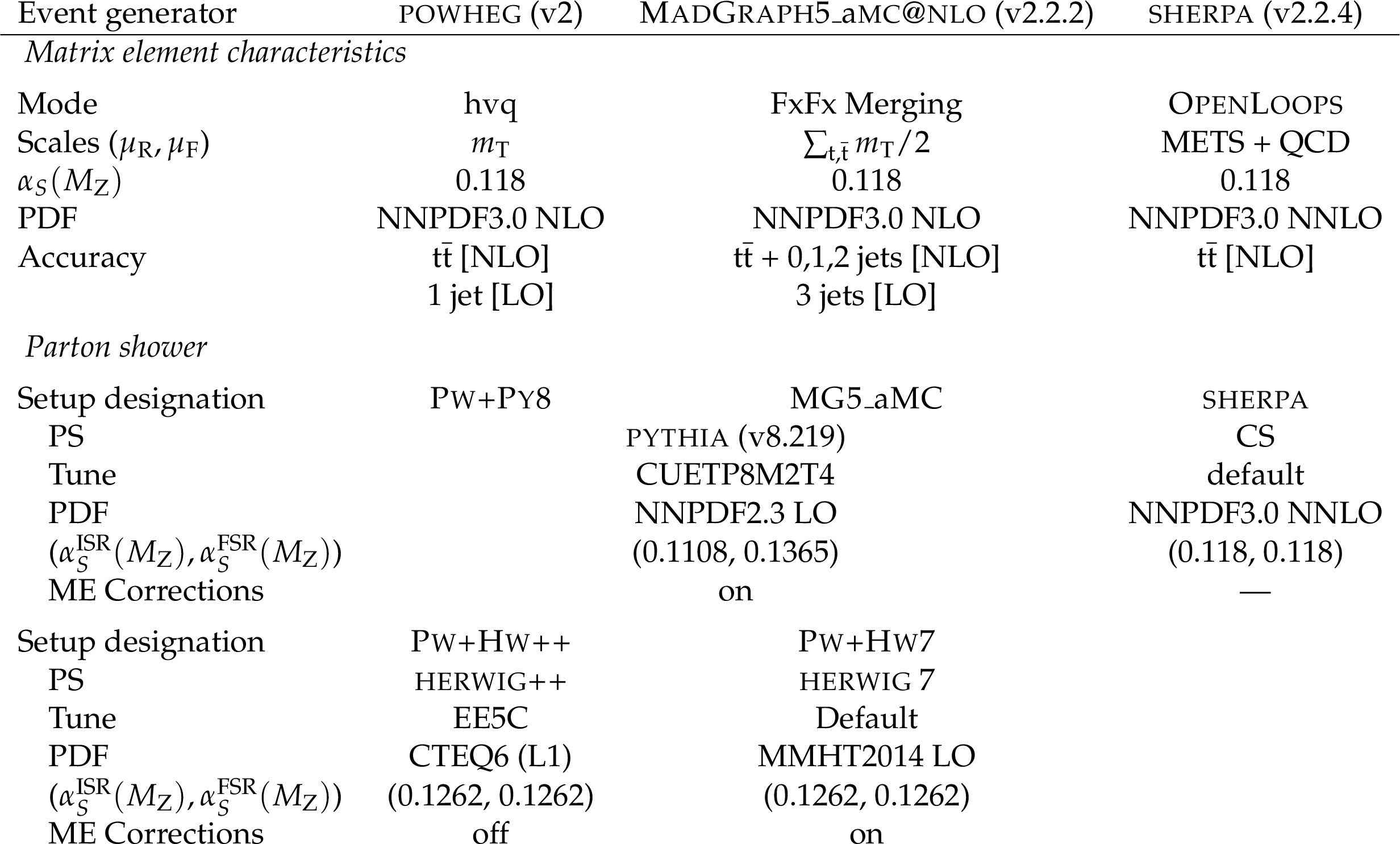
Table 1:
MC simulation settings used for the comparisons with the differential cross section measurements of the UE. The table lists the main characteristics and values used for the most relevant parameters of the generators. The row labeled "Setup designation'' shows the definitions of the abbreviations used throughout this paper. |

png pdf |
Table 2:
Uncertainties affecting the measurement of the average of the UE observables. The values are expressed in% and the last row reports the quadratic sum of the individual contributions. |
png pdf |
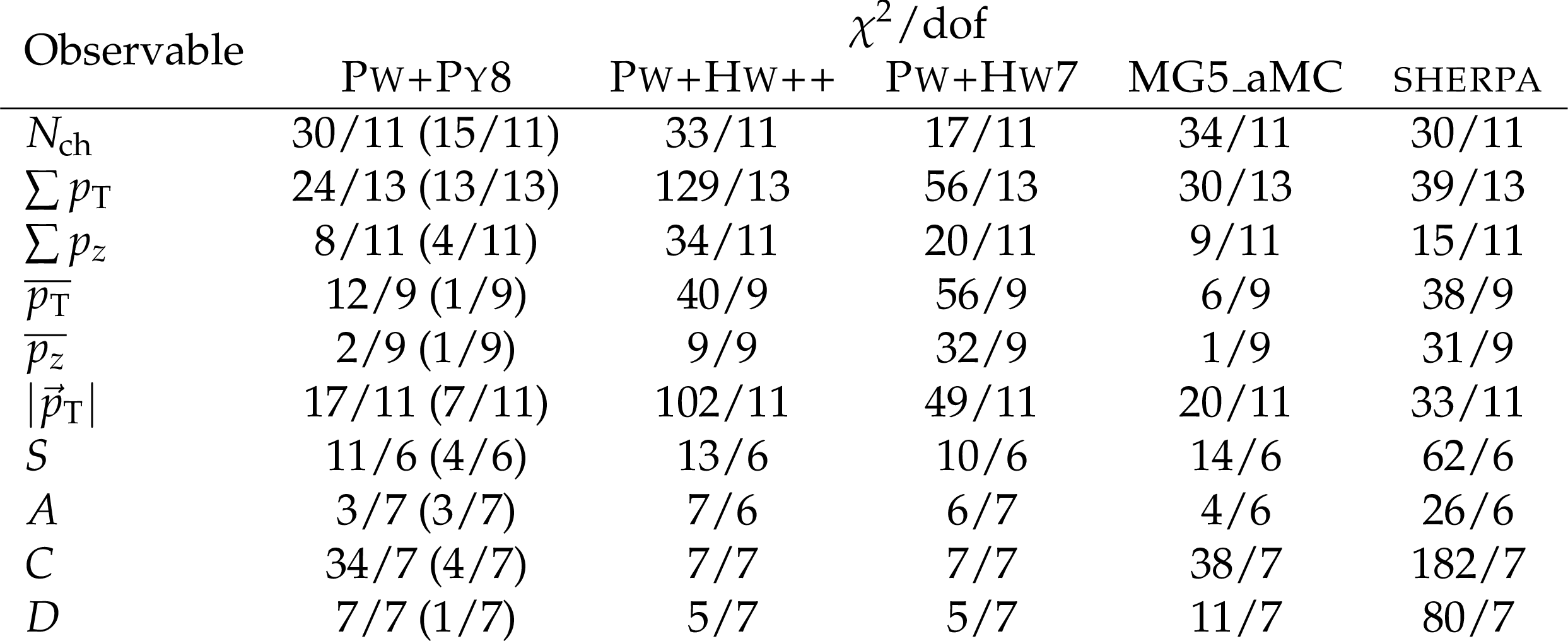
Table 3:
Comparison between the measured distributions at particle level and the predictions of different generator setups. We list the results of the $\chi ^2$ tests together with dof. For the comparison no uncertainties in the predictions are taken into account, except for the POWHEG+PYTHIA8 setup for which the comparison including the theoretical uncertainties is quoted separately in parenthesis. |

png pdf |
Table 4:
The first rows give the best fit values for $ {\alpha _S} ^\text {FSR}$ for the POWHEG+PYTHIA8 setup, obtained from the inclusive distribution of different observables and the corresponding 68 and 95% confidence intervals. The last two rows give the preferred value of the renormalization scale in units of $M_ {\mathrm {Z}}$, and the associated $ \pm $1$ \sigma $ interval that can be used as an estimate of its variation to encompass the differences between data and the POWHEG+PYTHIA8 setup. |
png pdf |
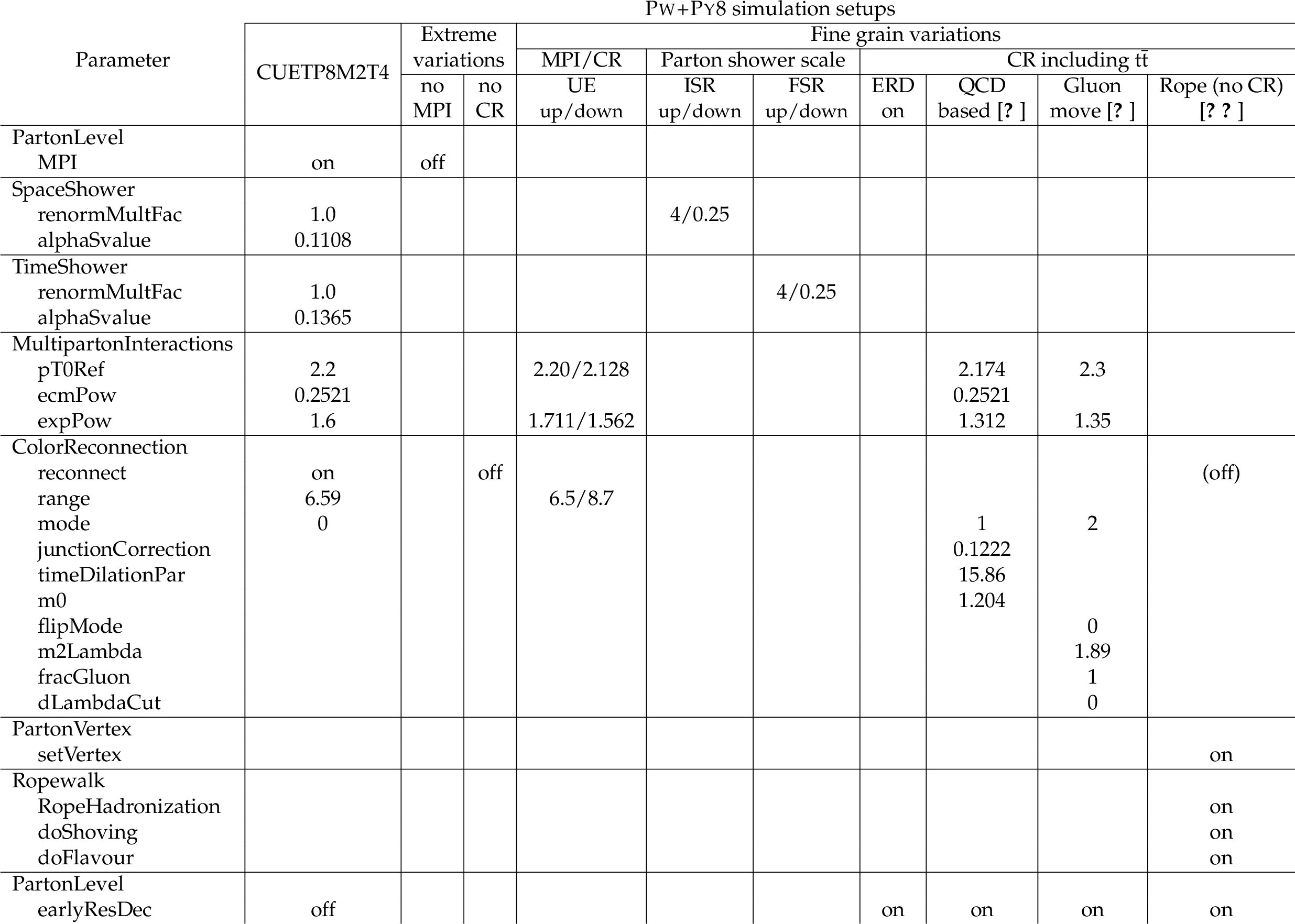
Table 5:
Variations of the POWHEG+PYTHIA8 setup used for the comparison with the measurements. The values changed with respect to the CUETP8M2T4 tune are given in the columns corresponding to each model. Further details on parameters or specificities of the models can be found in Ref. [16, 71, 3, 31, 31, 4, 32, 33]. For the Rope hadronization model two variations are considered: one with no CR and the other with the default CR model. The settings for the former are denoted in parenthesis in the last column. |
| Summary |
|
The first measurement of the underlying event (UE) activity in $\mathrm{t\bar{t}}$ dilepton events produced in hadron colliders has been reported. The measurement makes use of $\sqrt{s} = $ 13 TeV proton-proton collision data collected by the CMS experiment in 2016, and corresponding to 35.9 fb$^{-1}$. Using particle-flow reconstruction, the contribution from the UE has been isolated by removing charged particles associated with the decay products of the $\mathrm{t\bar{t}}$ event candidates as well as with pileup interactions from the set of reconstructed charged particles per event. The measurements performed are expected to be valid for other $\mathrm{t\bar{t}}$ final states, and can be used as a reference for complementary studies, eg, of how different color reconnection (CR) models compare to data in the description of the jets from $\mathrm{W}\to \mathrm{q}\mathrm{\bar{q}}'$ decays. The chosen observables and categories enhance the sensitivity to the modeling of multiparton interactions (MPI), CR and the choice of strong coupling parameter at the mass of Z boson (${\alpha_S}^\text{FSR}(M_\mathrm{Z})$) in the PYTHIA8 parton shower Monte Carlo simulation. These parameters have significant impact on the modeling of $\mathrm{t\bar{t}}$ production at the LHC. In particular, the compatibility of the data with different choices of the ${\alpha_S}^\text{FSR}(M_\mathrm{Z})$ parameter in PYTHIA8 has been quantified, resulting in a lower value than the one considered in Ref. [71]. The majority of the distributions analyzed indicate a fair agreement between the data and the POWHEG+PYTHIA8 setup with the CUETP8M2T4 tune [17], but disfavor the setups in which MPI and CR are switched off, or in which ${\alpha_S}^\text{FSR}(M_\mathrm{Z})$ is increased. The data also disfavor the default configurations in HERWIG++, HERWIG7, and SHERPA. It has been furthermore verified that, as expected, the choice of the next-to-leading-order matrix-element generator does not impact significantly the expected characteristics of the UE by comparing predictions from POWHEG and MadGraph5+MCatNLO, both interfaced with PYTHIA8. The present results test the hypothesis of universality in UE at an energy scale typically higher than the ones at which models have been studied. The UE model is tested up to a scale of two times the top quark mass, and the measurements in categories of dilepton invariant mass indicate that it should be valid at even higher scales. In addition, they can be used to improve the assessment of systematic uncertainties in future top quark analyses. The results obtained in this study show that a value of ${\alpha_S}^\text{FSR}(M_\mathrm{Z})=$ 0.120 $\pm$ 0.006 is consistent with the data. The corresponding uncertainties translate to a variation of the renormalization scale by a factor of $\sqrt{2}$. |
| References | ||||
| 1 | Particle Data Group | Review of particle physics | CPC 40 (2016) 100001 | |
| 2 | CMS Collaboration | Measurement of the top quark mass using charged particles in pp collisions at $ \sqrt s = $ 8 TeV | PRD 93 (2016) 092006 | CMS-TOP-12-030 1603.06536 |
| 3 | T. Sjostrand | Colour reconnection and its effects on precise measurements at the LHC | in Proceedings, 43rd International Symposium on Multiparticle Dynamics ISMD 13) 2013 C13-09-15.1 | 1310.8073 |
| 4 | S. Argyropoulos and T. Sjostrand | Effects of color reconnection on $ \mathrm{t\bar{t}} $ final states at the LHC | JHEP 11 (2014) 043 | 1407.6653 |
| 5 | G. Corcella | Interpretation of the top-quark mass measurements: a theory overview | in Proceedings, 8th International Workshop on Top Quark Physics (TOP2015), volume TOP2015, p. 037 Ischia, Italy, September, 2016 PoS(TOP2015)037 | 1511.08429 |
| 6 | G. Corcella, R. Franceschini, and D. Kim | Fragmentation uncertainties in hadronic observables for top-quark mass measurements | NPB 929 (2018) 485 | 1712.05801 |
| 7 | S. Ferrario Ravasio, T. Je\vzo, P. Nason, and C. Oleari | A theoretical study of top-mass measurements at the LHC using NLO+PS generators of increasing accuracy | 1801.03944 | |
| 8 | CMS Collaboration | Particle-flow reconstruction and global event description with the CMS detector | JINST 12 (2017) P10003 | CMS-PRF-14-001 1706.04965 |
| 9 | CMS Collaboration | The CMS trigger system | JINST 12 (2017) P01020 | CMS-TRG-12-001 1609.02366 |
| 10 | CMS Collaboration | The CMS experiment at the CERN LHC | JINST 3 (2008) S08004 | CMS-00-001 |
| 11 | CMS Collaboration | CMS luminosity measurements for the 2016 data taking period | CMS-PAS-LUM-17-001 | CMS-PAS-LUM-17-001 |
| 12 | P. Nason | A new method for combining NLO QCD with shower Monte Carlo algorithms | JHEP 11 (2004) 040 | hep-ph/0409146 |
| 13 | S. Frixione, P. Nason, and C. Oleari | Matching NLO QCD computations with parton shower simulations: the POWHEG method | JHEP 11 (2007) 070 | 0709.2092 |
| 14 | S. Alioli, P. Nason, C. Oleari, and E. Re | A general framework for implementing NLO calculations in shower Monte Carlo programs: the POWHEG BOX | JHEP 06 (2010) 043 | 1002.2581 |
| 15 | NNPDF Collaboration | Parton distributions for the LHC run ii | JHEP 04 (2015) 040 | 1410.8849 |
| 16 | T. Sjostrand et al. | An introduction to PYTHIA 8.2 | CPC 191 (2015) 159 | 1410.3012 |
| 17 | CMS Collaboration | Investigations of the impact of the parton shower tuning in $ PYTHIA8 $ in the modelling of $ \mathrm{t\overline{t}} $ at $ \sqrt{s}= $ 8 and 13 TeV | CMS-PAS-TOP-16-021 | CMS-PAS-TOP-16-021 |
| 18 | CMS Collaboration | Event generator tunes obtained from underlying event and multiparton scattering measurements | EPJC 76 (2016) 155 | CMS-GEN-14-001 1512.00815 |
| 19 | CMS Collaboration | Measurement of $ \mathrm {t}\overline{\mathrm {t}} $ production with additional jet activity, including $ \mathrm {b} $ quark jets, in the dilepton decay channel using pp collisions at $ \sqrt{s}= $ 8 TeV | EPJC 76 (2016) 379 | CMS-TOP-12-041 1510.03072 |
| 20 | M. Czakon and A. Mitov | Top++: A program for the calculation of the top-pair cross-section at hadron colliders | CPC 185 (2014) 2930 | 1112.5675 |
| 21 | J. Alwall et al. | The automated computation of tree-level and next-to-leading order differential cross sections, and their matching to parton shower simulations | JHEP 07 (2014) 079 | 1405.0301 |
| 22 | R. Frederix and S. Frixione | Merging meets matching in MC@NLO | JHEP 12 (2012) 061 | 1209.6215 |
| 23 | T. Gleisberg et al. | Event generation with SHERPA 1.1 | JHEP 02 (2009) 007 | 0811.4622 |
| 24 | F. Cascioli, P. Maierhofer, and S. Pozzorini | Scattering amplitudes with open loops | PRL 108 (2012) 111601 | 1111.5206 |
| 25 | S. Schumann and F. Krauss | A parton shower algorithm based on Catani-Seymour dipole factorisation | JHEP 03 (2008) 038 | 0709.1027 |
| 26 | M. Bahr et al. | Herwig++ physics and manual | EPJC 58 (2008) 639 | 0803.0883 |
| 27 | M. H. Seymour and A. Siodmok | Constraining MPI models using $ \sigma_{eff} $ and recent tevatron and LHC underlying event data | JHEP 10 (2013) 113 | 1307.5015 |
| 28 | J. Pumplin et al. | New generation of parton distributions with uncertainties from global QCD analysis | JHEP 07 (2002) 012 | hep-ph/0201195 |
| 29 | J. Bellm et al. | Herwig 7.0/Herwig++ 3.0 release note | EPJC 76 (2016) 196 | 1512.01178 |
| 30 | L. A. Harland-Lang, A. D. Martin, P. Motylinski, and R. S. Thorne | Parton distributions in the LHC era: MMHT 2014 PDFs | EPJC 75 (2015) 204 | 1412.3989 |
| 31 | J. R. Christiansen and P. Z. Skands | String formation beyond leading colour | JHEP 08 (2015) 003 | 1505.01681 |
| 32 | C. Bierlich, G. Gustafson, L. Lonnblad, and A. Tarasov | Effects of overlapping strings in pp collisions | JHEP 03 (2015) 148 | 1412.6259 |
| 33 | C. Bierlich and J. R. Christiansen | Effects of color reconnection on hadron flavor observables | PRD 92 (2015) 094010 | 1507.02091 |
| 34 | J. Alwall et al. | Comparative study of various algorithms for the merging of parton showers and matrix elements in hadronic collisions | EPJC 53 (2008) 473 | 0706.2569 |
| 35 | T. Melia, P. Nason, R. Rontsch, and G. Zanderighi | $ \mathrm{W}^+ \mathrm{W}^- $, WZ and ZZ production in the POWHEG BOX | JHEP 11 (2011) 078 | 1107.5051 |
| 36 | P. Nason and G. Zanderighi | $ \mathrm{W}^+ \mathrm{W}^- $ , WZ and ZZ production in the POWHEG-BOX-V2 | EPJC 74 (2014), no. 1 | 1311.1365 |
| 37 | E. Re | Single-top Wt-channel production matched with parton showers using the POWHEG method | EPJC 71 (2011) 1547 | 1009.2450 |
| 38 | S. Alioli, P. Nason, C. Oleari, and E. Re | NLO single-top production matched with shower in POWHEG: $ s $- and $ t $-channel contributions | JHEP 09 (2009) 111 | 0907.4076 |
| 39 | P. Artoisenet, R. Frederix, O. Mattelaer, and R. Rietkerk | Automatic spin-entangled decays of heavy resonances in Monte Carlo simulations | JHEP 03 (2013) 015 | 1212.3460 |
| 40 | K. Melnikov and F. Petriello | Electroweak gauge boson production at hadron colliders through $ O(\alpha_s^2) $ | PRD 74 (2006) 114017 | hep-ph/0609070 |
| 41 | N. Kidonakis | Top quark production | in Proceedings, Helmholtz International Summer School on Physics of Heavy Quarks and Hadrons (HQ 2013): JINR, Dubna, Russia, July 15-28, 2013, p. 139 2014 | 1311.0283 |
| 42 | T. Gehrmann et al. | W$ ^+ $W$ ^- $ production at hadron colliders in next to next to leading order QCD | PRL 113 (2014) 212001 | 1408.5243 |
| 43 | GEANT4 Collaboration | $ GEANT4--a $ simulation toolkit | NIMA 506 (2003) 250 | |
| 44 | GEANT4 Collaboration | $ GEANT4 $ developments and applications | IEEE Trans. Nucl. Sci. 53 (2006) 270 | |
| 45 | GEANT4 Collaboration | Recent developments in $ GEANT4 $ | NIMA 835 (2016) 186 | |
| 46 | CMS Collaboration | Measurement of the $ \rm \mathrm{t\bar{t}} $ production cross section using events in the e$ \mu $ final state in pp collisions at $ \sqrt{s} = $ 13 TeV | EPJC 77 (2017) 172 | CMS-TOP-16-005 1611.04040 |
| 47 | CMS Collaboration | Measurements of inclusive W and Z cross sections in pp collisions at $ \sqrt{s}= $ 7 TeV | JHEP 01 (2011) 080 | CMS-EWK-10-002 1012.2466 |
| 48 | M. Cacciari, G. P. Salam, and G. Soyez | The anti-$ {k_{\mathrm{T}}} $ jet clustering algorithm | JHEP 04 (2008) 063 | 0802.1189 |
| 49 | M. Cacciari, G. P. Salam, and G. Soyez | FastJet user manual | EPJC 72 (2012) 1896 | 1111.6097 |
| 50 | CMS Collaboration | Jet energy scale and resolution in the CMS experiment in pp collisions at 8 TeV | JINST 12 (2017) P02014 | CMS-JME-13-004 1607.03663 |
| 51 | CMS Collaboration | Identification of heavy-flavour jets with the CMS detector in pp collisions at 13 TeV | JINST 13 (2018) P05011 | CMS-BTV-16-002 1712.07158 |
| 52 | CMS Collaboration | First measurement of the cross section for top-quark pair production in proton-proton collisions at $ \sqrt{s}= $ 7 TeV | PLB 695 (2011) 424 | CMS-TOP-10-001 1010.5994 |
| 53 | CMS Collaboration | Object definitions for top quark analyses at the particle level | CDS | |
| 54 | A. Buckley et al. | Rivet user manual | CPC 184 (2013) 2803 | 1003.0694 |
| 55 | G. Parisi | Superinclusive cross sections | PLB 74 (1978) 65 | |
| 56 | J. F. Donoghue, F. E. Low, and S.-Y. Pi | Tensor analysis of hadronic jets in quantum chromodynamics | PRD 20 (1979) 2759 | |
| 57 | R. K. Ellis, D. A. Ross, and A. E. Terrano | The perturbative calculation of jet structure in e$ ^+ $e$ ^- $ annihilation | NPB 178 (1981) 421 | |
| 58 | CMS Collaboration | Description and performance of track and primary-vertex reconstruction with the CMS tracker | JINST 9 (2014) P10009 | CMS-TRK-11-001 1405.6569 |
| 59 | A. N. Tikhonov | Solution of incorrectly formulated problems and the regularization method | Soviet Math. Dokl. 4 (1963) 1035 | |
| 60 | S. Schmitt | TUnfold: an algorithm for correcting migration effects in high energy physics | JINST 7 (2012) T10003 | 1205.6201 |
| 61 | CMS Collaboration | Measurement of the inelastic proton-proton cross section at $ \sqrt{s}= $ 13 TeV | Submitted to JHEP | CMS-FSQ-15-005 1802.02613 |
| 62 | CMS Collaboration | Performance of electron reconstruction and selection with the cms detector in proton-proton collisions at $ \sqrt{s} = $ 8 TeV | JINST 10 (2015) P06005 | CMS-EGM-13-001 1502.02701 |
| 63 | CMS Collaboration | Performance of CMS muon reconstruction in pp collision events at $ \sqrt{s}= $ 7 TeV | JINST 7 (2012) P10002 | CMS-MUO-10-004 1206.4071 |
| 64 | CMS Collaboration | Tracking POG plot results on 2015 data | CDS | |
| 65 | M. Cacciari et al. | The $ \mathrm{t\bar{t}} $ cross-section at 1.8 TeV and 1.96 TeV: a study of the systematics due to parton densities and scale dependence | JHEP 04 (2004) 068 | hep-ph/0303085 |
| 66 | S. Catani, D. de Florian, M. Grazzini, and P. Nason | Soft gluon resummation for Higgs boson production at hadron colliders | JHEP 07 (2003) 028 | hep-ph/0306211 |
| 67 | CMS Collaboration | Measurement of differential cross sections for top quark pair production using the lepton+jets final state in proton-proton collisions at 13 TeV | PRD 95 (2017) 092001 | CMS-TOP-16-008 1610.04191 |
| 68 | CMS Collaboration | Measurement of normalized differential $ \mathrm{t}\overline{\mathrm{t}} $ cross sections in the dilepton channel from pp collisions at $ \sqrt{s}= $ 13 TeV | JHEP 04 (2018) 060 | CMS-TOP-16-007 1708.07638 |
| 69 | CMS Collaboration | Measurement of the top quark mass using proton-proton data at $ {\sqrt{s}} = $ 7 and 8 TeV | PRD 93 (2016) 072004 | CMS-TOP-14-022 1509.04044 |
| 70 | F. James | World Scientific, Hackensack, NJ, 2006 ,ISBN 9789812567956 | ||
| 71 | P. Skands, S. Carrazza, and J. Rojo | Tuning PYTHIA 8.1: the Monash 2013 tune | EPJC 74 (2014) 3024 | 1404.5630 |
|
|
Compact Muon Solenoid LHC, CERN |
|

|

|

|

|

|