CMS-EXO-21-018

CMS-EXO-21-018 ; CERN-EP-2023-304
Search for a scalar or pseudoscalar dilepton resonance produced in association with a massive vector boson or top quark-antiquark pair in multilepton events at $ \sqrt{s} = $ 13 TeV
CMS Collaboration
16 February 2024
Submitted to Phys. Rev. D
Abstract: A search for beyond the standard model spin-0 bosons, $ \phi $, that decay into pairs of electrons, muons, or tau leptons is presented. The search targets the associated production of such bosons with a W or Z gauge boson, or a top quark-antiquark pair, and uses events with three or four charged leptons, including hadronically decaying tau leptons. The proton-proton collision data set used in the analysis was collected at the LHC from 2016 to 2018 at a center-of-mass energy of 13 TeV, and corresponds to an integrated luminosity of 138 fb$ ^{-1} $. The observations are consistent with the predictions from standard model processes. Upper limits are placed on the product of cross sections and branching fractions of such new particles over the mass range of 15 to 350 GeV with scalar, pseudoscalar, or Higgs-boson-like couplings, as well as on the product of coupling parameters and branching fractions. Several model-dependent exclusion limits are also presented. For a Higgs-boson-like $ \phi $ model, limits are set on the mixing angle of the Higgs boson with the $ \phi $ boson. For the associated production of a $ \phi $ boson with a top quark-antiquark pair, limits are set on the coupling to top quarks. Finally, limits are set for the first time on a fermiophilic dilaton-like model with scalar couplings and a fermiophilic axion-like model with pseudoscalar couplings.
Links: e-print arXiv:2402.11098 [hep-ex] (PDF) ; CDS record ; inSPIRE record ; HepData record ; CADI line (restricted) ;

Figures & Tables	Summary	Additional Figures	References	CMS Publications

Figures
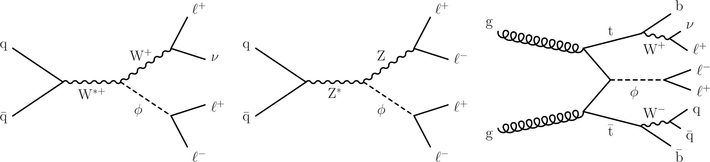
png pdf	Figure 1: Example production and decay processes of $ {\mathrm{W}}{\phi} $, $ {\mathrm{Z}}{\phi} $, and $ {{\mathrm{t}\overline{\mathrm{t}}} }{\phi} $ signals with multilepton final states, where $ \ell $ stands for electron, muon or tau lepton. Only leptonic decays of W and Z bosons are considered for $ {\mathrm{W}}{\phi} $ and $ {\mathrm{Z}}{\phi} $ signals, while for the $ {{\mathrm{t}\overline{\mathrm{t}}} }{\phi} $ signal, W bosons from top quark decay can also decay hadronically.
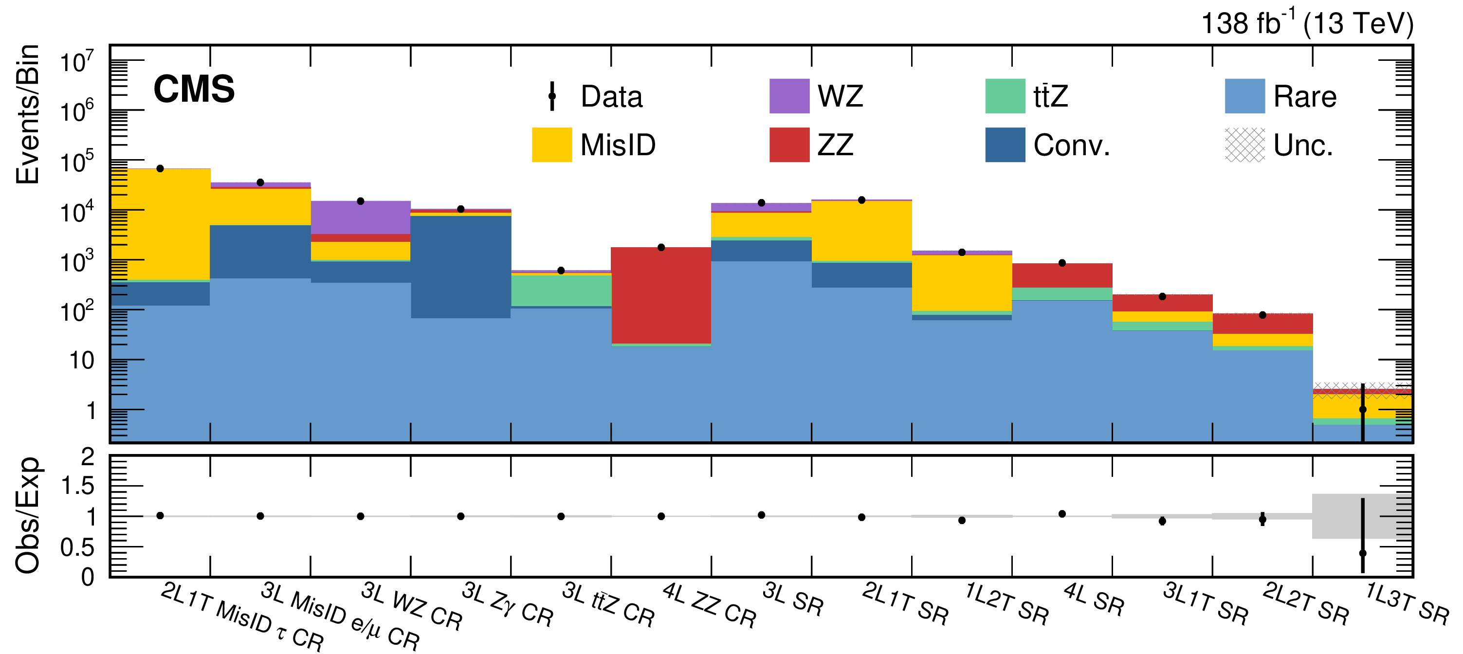
png pdf	Figure 2: Binned representation of the control and signal regions for the combined multilepton event selection and the combined 2016-2018 data set. The CR bins follow their definitions as given in Table 1, and the SR bins correspond to the channels as defined by the lepton flavor composition. The normalizations of the background samples in the CRs are described in Sections 5.1 and 5.2. All three (four) lepton events are required to have $ Q_{\ell}=1 (0) $, and those satisfying any of the CR requirements are removed from the SR bins. All subsequent selections given in Tables 2 and 3 are based on events given in the SR bins. The lower panel shows the ratio of observed events to the total expected SM background prediction (Obs/Exp), and the gray band represents the statistical uncertainties in the background prediction.
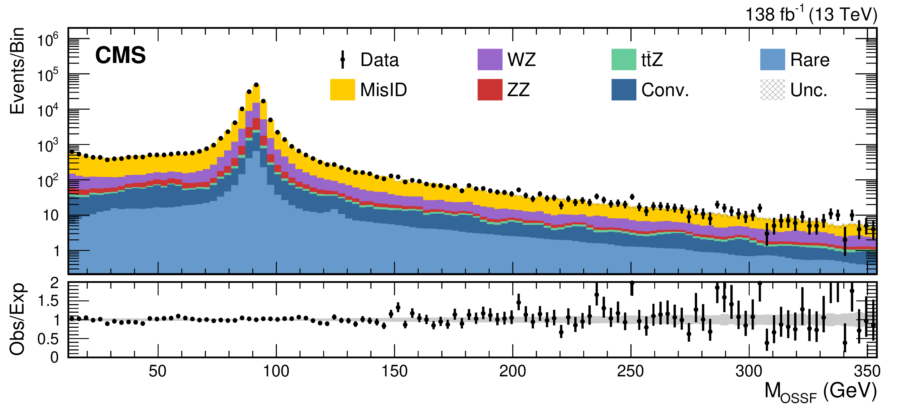
png pdf	Figure 3: The $ M_{\mathrm{OSSF}} $ spectrum for the combined 2L1T, 2L2T, 3L, 3L1T, and 4L event selection (excluding the $ {\mathrm{Z}}{\gamma} $ CR) and the combined 2016-2018 data set. All three (four) lepton events are required to have $ Q_{\ell}=1\,(0) $. The lower panel shows the ratio of observed events to the total expected SM background prediction (Obs/Exp), and the gray band represents the statistical uncertainties in the background prediction.
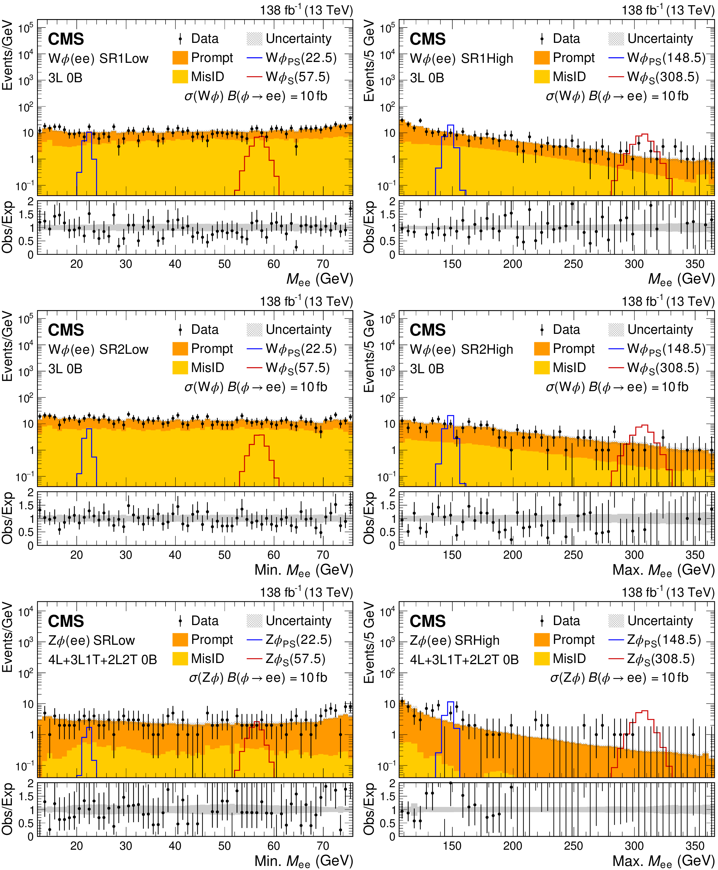
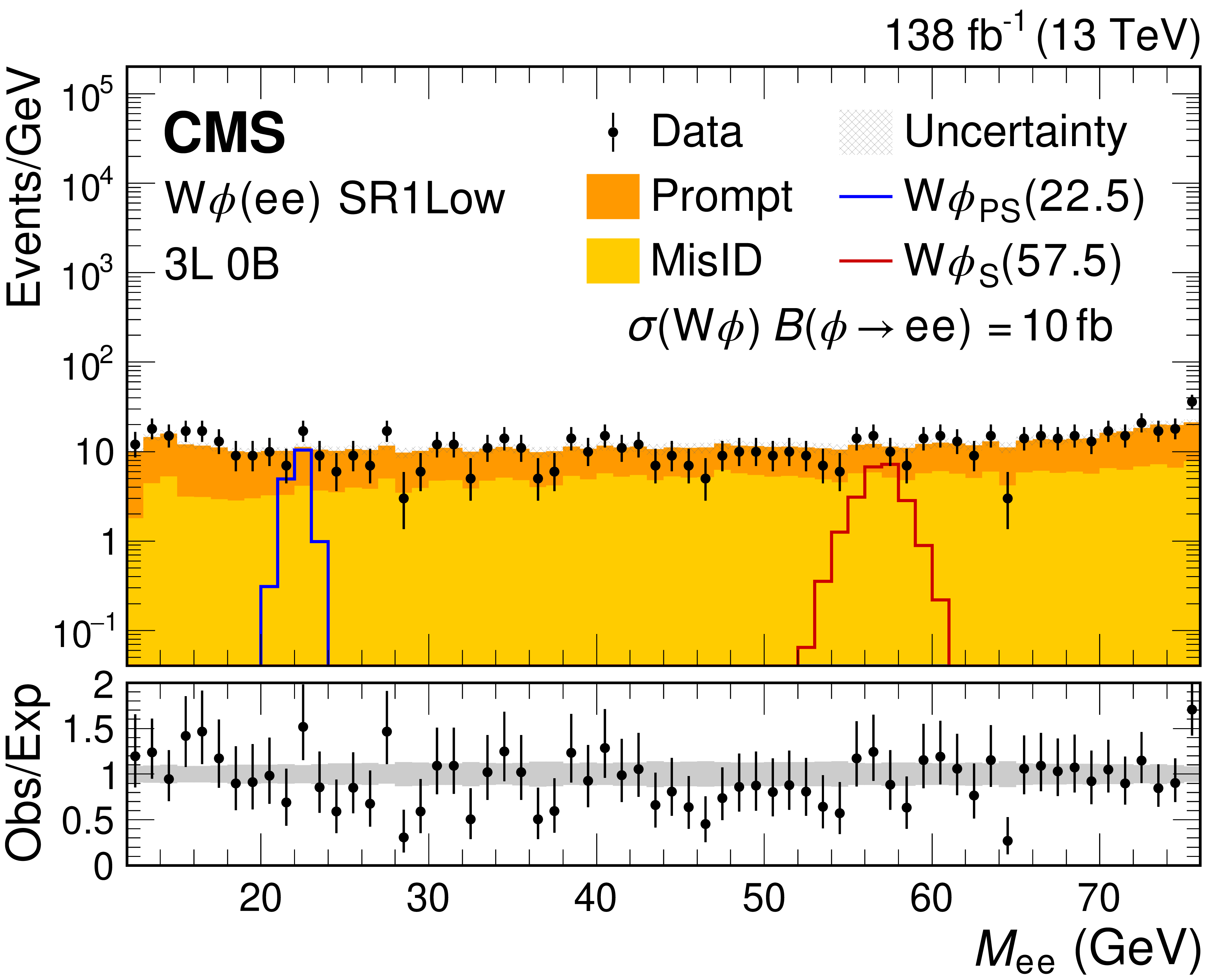
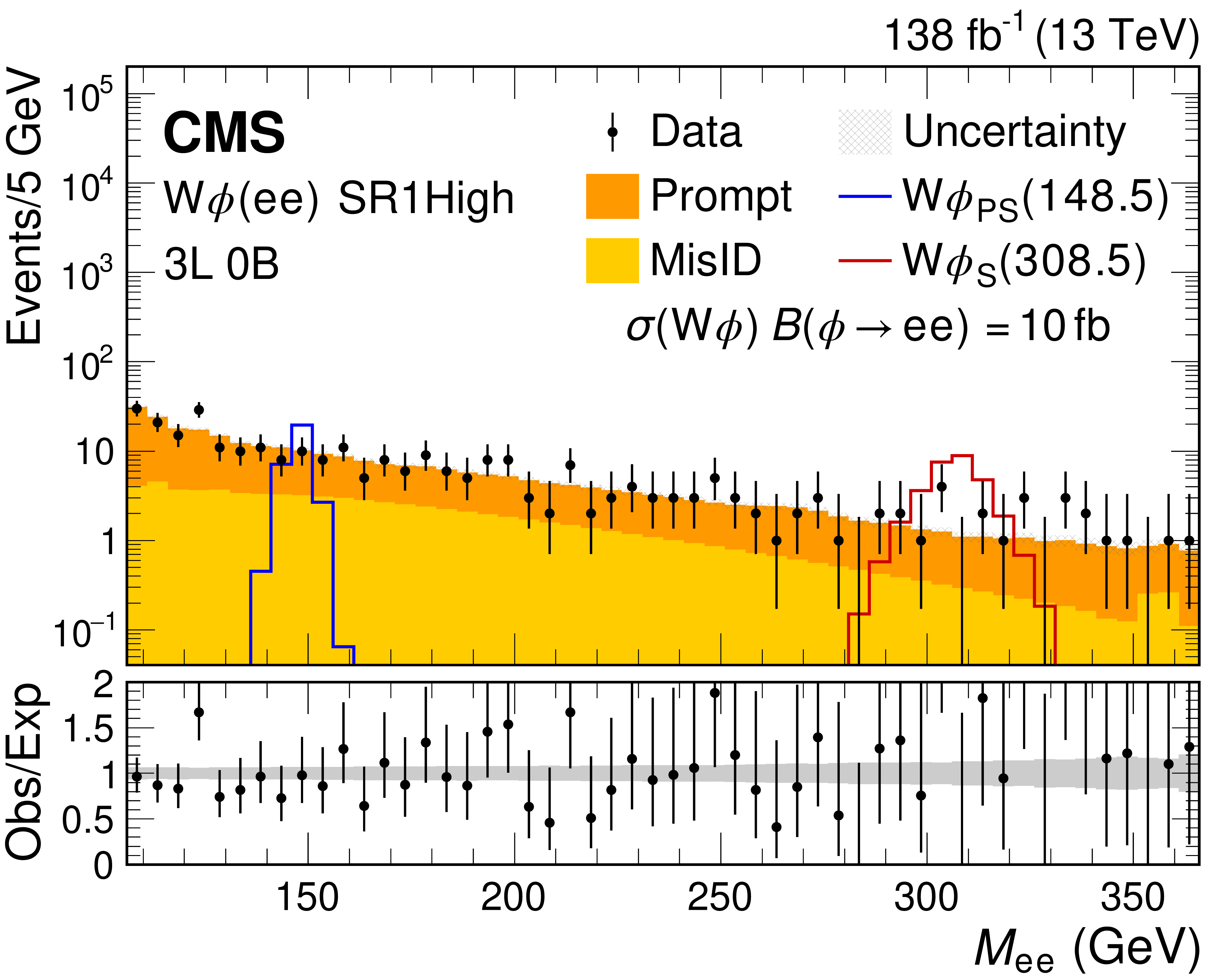
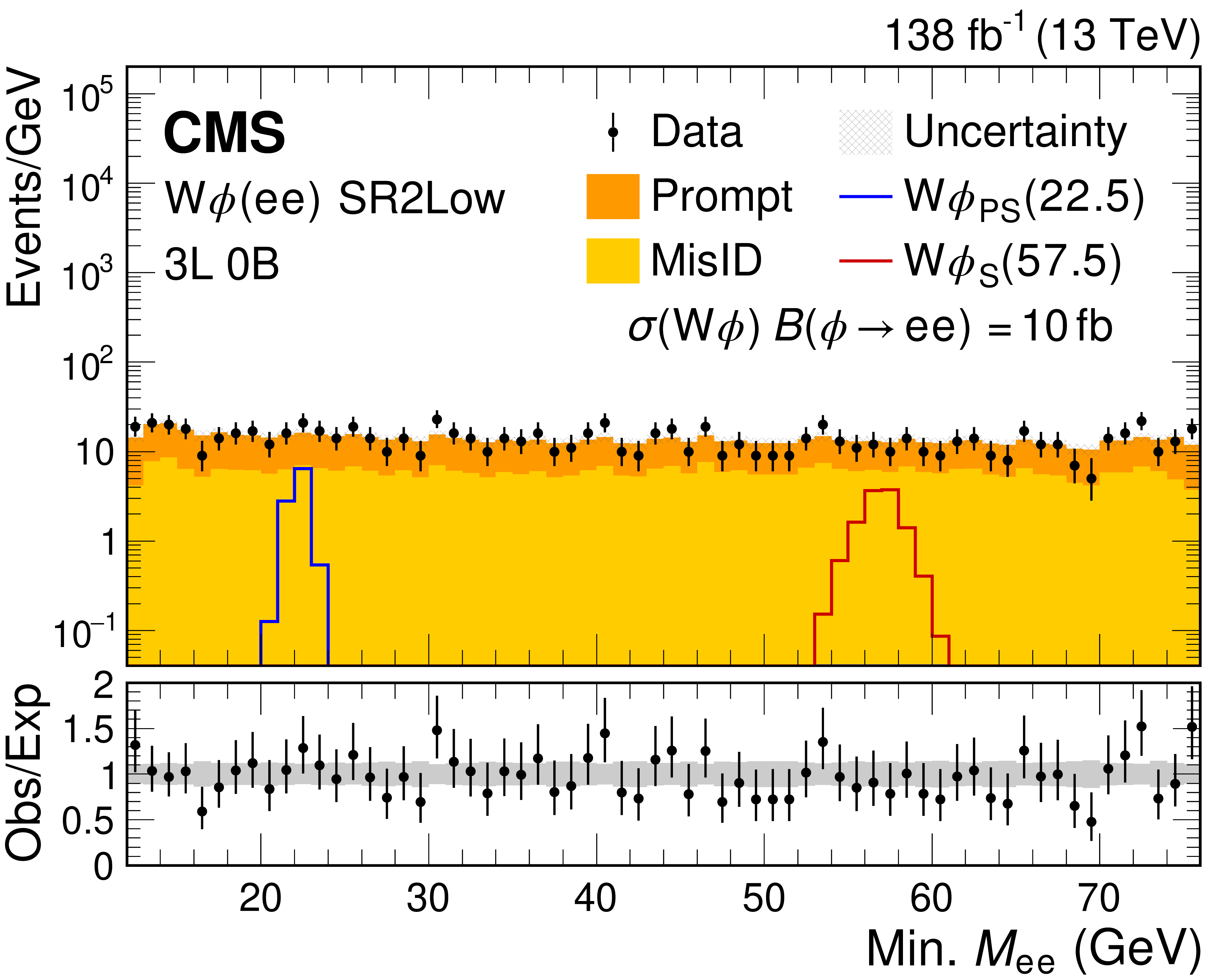
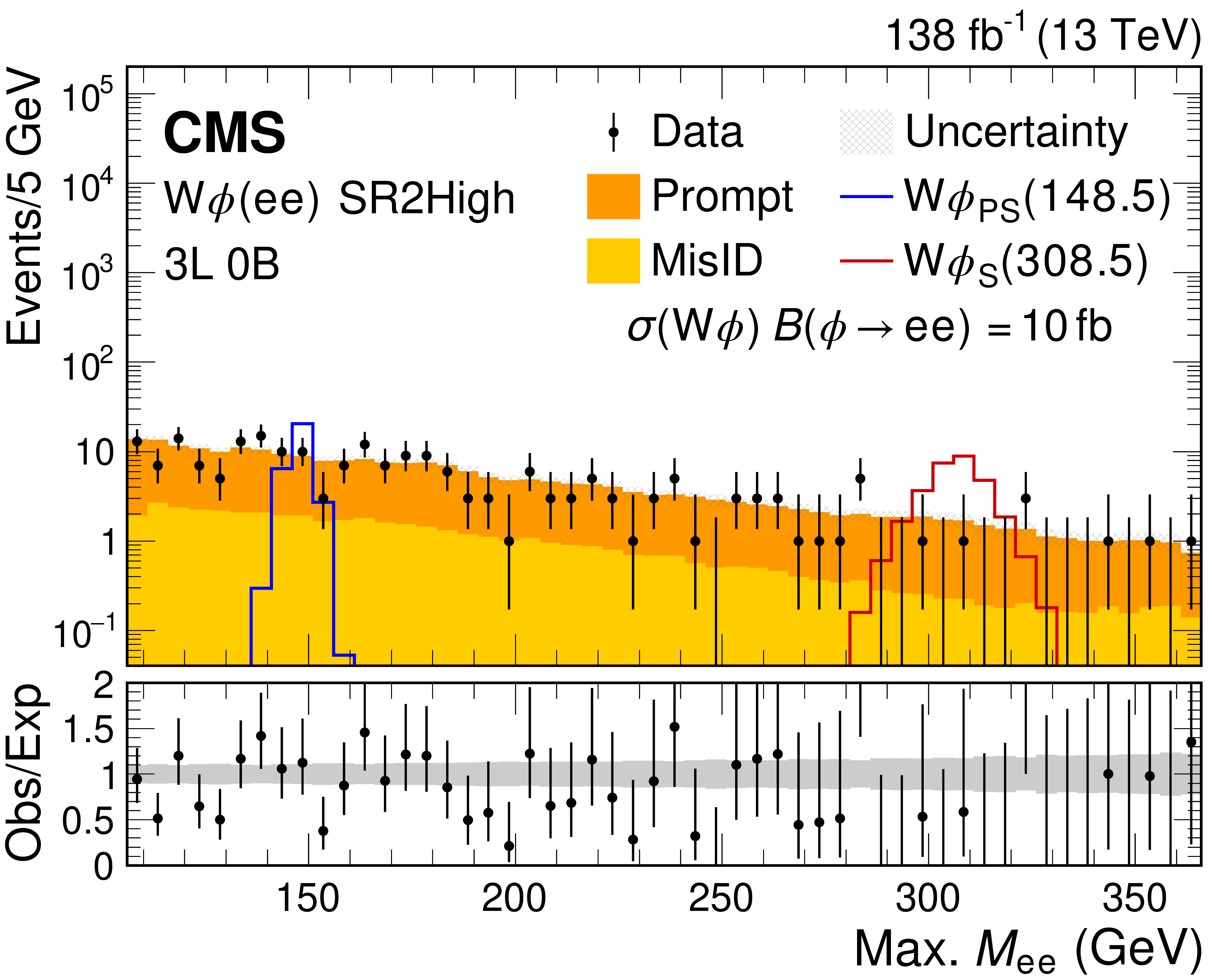
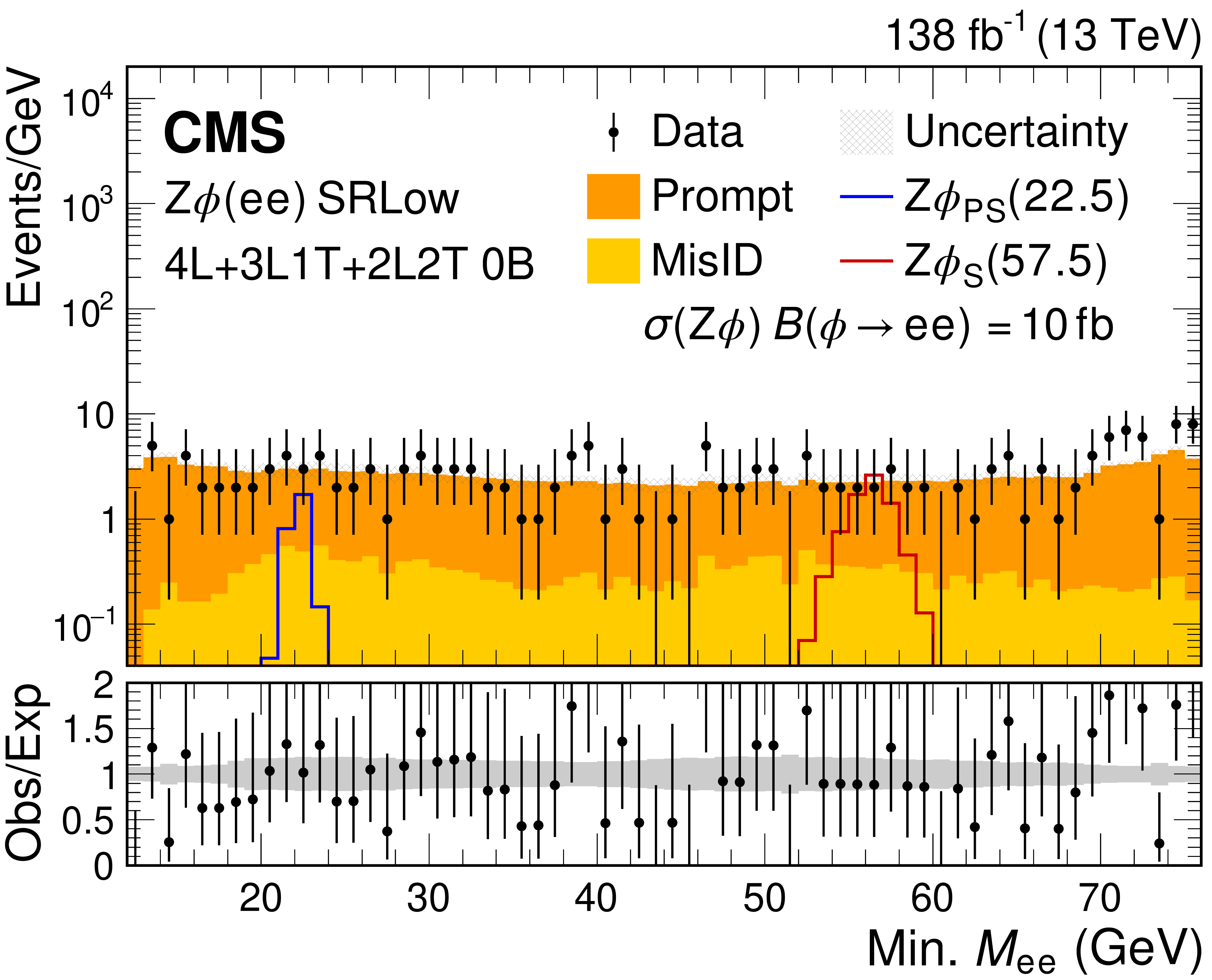
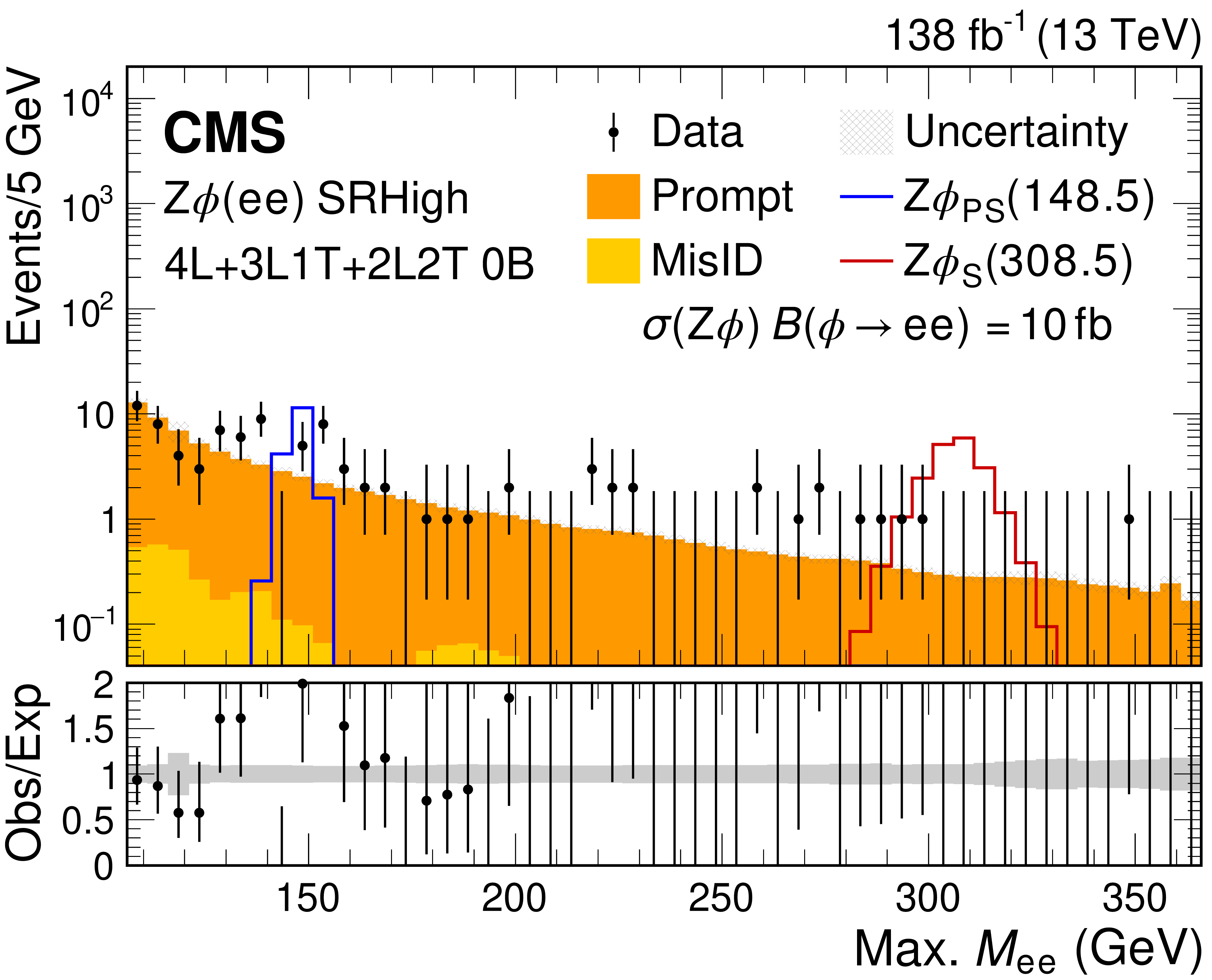
png pdf	Figure 4: Dilepton mass spectra for the $ {\mathrm{W}}{\phi}(\mathrm{e}\mathrm{e}) $ SR1 (upper), SR2 (middle), and for the $ {\mathrm{Z}}{\phi}(\mathrm{e}\mathrm{e}) $ SR (lower) event selections for the combined 2016-2018 data set. The low (high) mass spectra are shown on the left (right). The lower panel shows the ratio of observed events to the total expected SM background prediction (Obs/Exp), and the gray band represents the sum of statistical and systematic uncertainties in the background prediction. The expected background distributions and the uncertainties are shown after the data is fit under the background-only hypothesis. For illustration, two example signal hypotheses for the production and decay of a scalar and a pseudoscalar $ \phi $ boson are shown, and their masses (in units of GeV) are indicated in the legend. The signals are normalized to the product of the cross section and branching fraction of 10 fb.
png pdf	Figure 4-a: Dilepton low mass spectrum for the $ {\mathrm{W}}{\phi}(\mathrm{e}\mathrm{e}) $ SR1 event selection for the combined 2016-2018 data set. The lower panel shows the ratio of observed events to the total expected SM background prediction (Obs/Exp), and the gray band represents the sum of statistical and systematic uncertainties in the background prediction. The expected background distributions and the uncertainties are shown after the data is fit under the background-only hypothesis. For illustration, two example signal hypotheses for the production and decay of a scalar and a pseudoscalar $ \phi $ boson are shown, and their masses (in units of GeV) are indicated in the legend. The signals are normalized to the product of the cross section and branching fraction of 10 fb.
png pdf	Figure 4-b: Dilepton high mass spectrum for the $ {\mathrm{W}}{\phi}(\mathrm{e}\mathrm{e}) $ SR1 event selection for the combined 2016-2018 data set. The lower panel shows the ratio of observed events to the total expected SM background prediction (Obs/Exp), and the gray band represents the sum of statistical and systematic uncertainties in the background prediction. The expected background distributions and the uncertainties are shown after the data is fit under the background-only hypothesis. For illustration, two example signal hypotheses for the production and decay of a scalar and a pseudoscalar $ \phi $ boson are shown, and their masses (in units of GeV) are indicated in the legend. The signals are normalized to the product of the cross section and branching fraction of 10 fb.
png pdf	Figure 4-c: Dilepton low mass spectrum for the $ {\mathrm{W}}{\phi}(\mathrm{e}\mathrm{e}) $ SR2 event selection for the combined 2016-2018 data set. The lower panel shows the ratio of observed events to the total expected SM background prediction (Obs/Exp), and the gray band represents the sum of statistical and systematic uncertainties in the background prediction. The expected background distributions and the uncertainties are shown after the data is fit under the background-only hypothesis. For illustration, two example signal hypotheses for the production and decay of a scalar and a pseudoscalar $ \phi $ boson are shown, and their masses (in units of GeV) are indicated in the legend. The signals are normalized to the product of the cross section and branching fraction of 10 fb.
png pdf	Figure 4-d: Dilepton high mass spectrum for the $ {\mathrm{W}}{\phi}(\mathrm{e}\mathrm{e}) $ SR2 event selection for the combined 2016-2018 data set. The lower panel shows the ratio of observed events to the total expected SM background prediction (Obs/Exp), and the gray band represents the sum of statistical and systematic uncertainties in the background prediction. The expected background distributions and the uncertainties are shown after the data is fit under the background-only hypothesis. For illustration, two example signal hypotheses for the production and decay of a scalar and a pseudoscalar $ \phi $ boson are shown, and their masses (in units of GeV) are indicated in the legend. The signals are normalized to the product of the cross section and branching fraction of 10 fb.
png pdf	Figure 4-e: Dilepton low mass spectrum for the $ {\mathrm{Z}}{\phi}(\mathrm{e}\mathrm{e}) $ SR event selection for the combined 2016-2018 data set. The lower panel shows the ratio of observed events to the total expected SM background prediction (Obs/Exp), and the gray band represents the sum of statistical and systematic uncertainties in the background prediction. The expected background distributions and the uncertainties are shown after the data is fit under the background-only hypothesis. For illustration, two example signal hypotheses for the production and decay of a scalar and a pseudoscalar $ \phi $ boson are shown, and their masses (in units of GeV) are indicated in the legend. The signals are normalized to the product of the cross section and branching fraction of 10 fb.
png pdf	Figure 4-f: Dilepton high mass spectrum for the $ {\mathrm{Z}}{\phi}(\mathrm{e}\mathrm{e}) $ SR event selection for the combined 2016-2018 data set. The lower panel shows the ratio of observed events to the total expected SM background prediction (Obs/Exp), and the gray band represents the sum of statistical and systematic uncertainties in the background prediction. The expected background distributions and the uncertainties are shown after the data is fit under the background-only hypothesis. For illustration, two example signal hypotheses for the production and decay of a scalar and a pseudoscalar $ \phi $ boson are shown, and their masses (in units of GeV) are indicated in the legend. The signals are normalized to the product of the cross section and branching fraction of 10 fb.
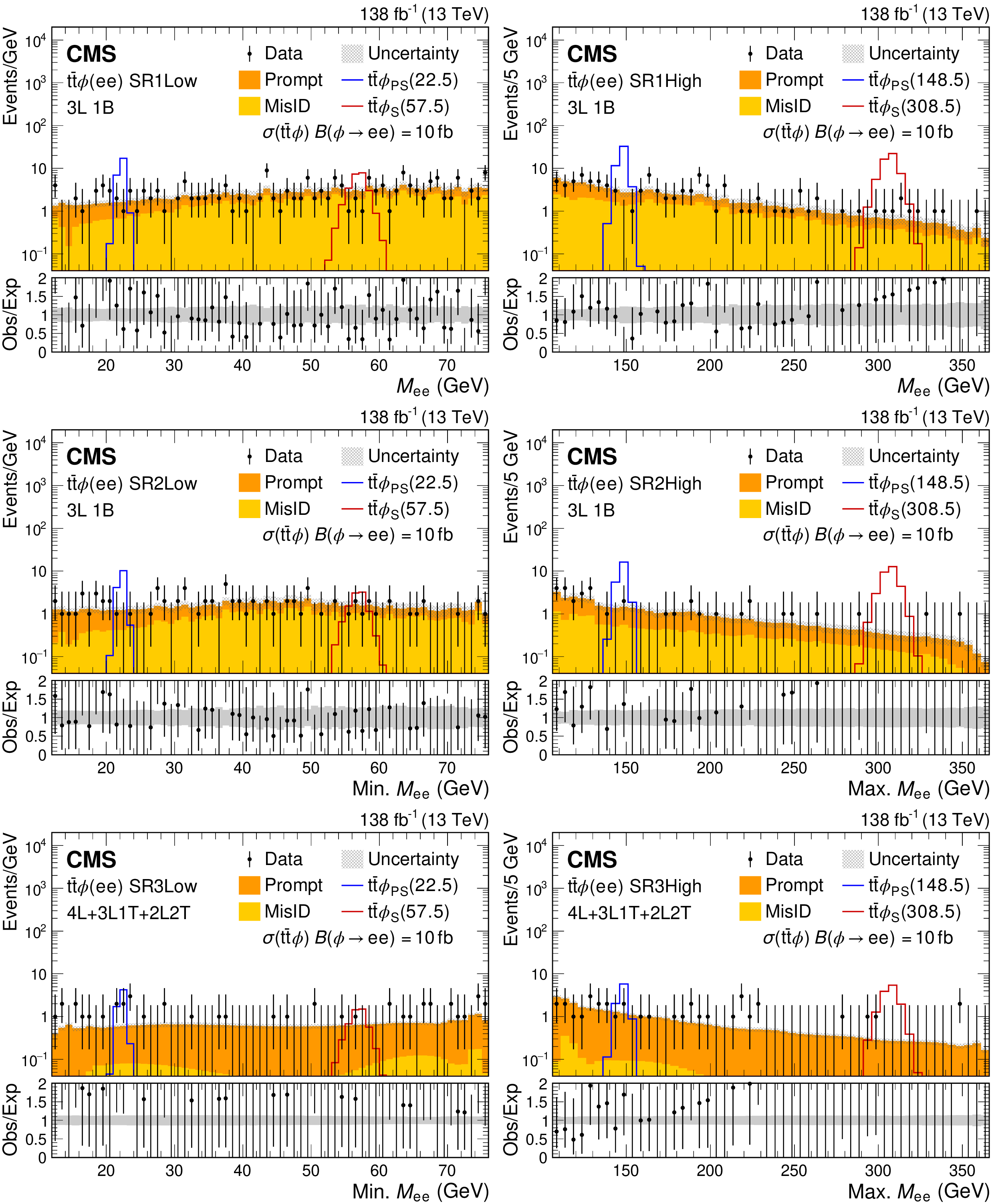
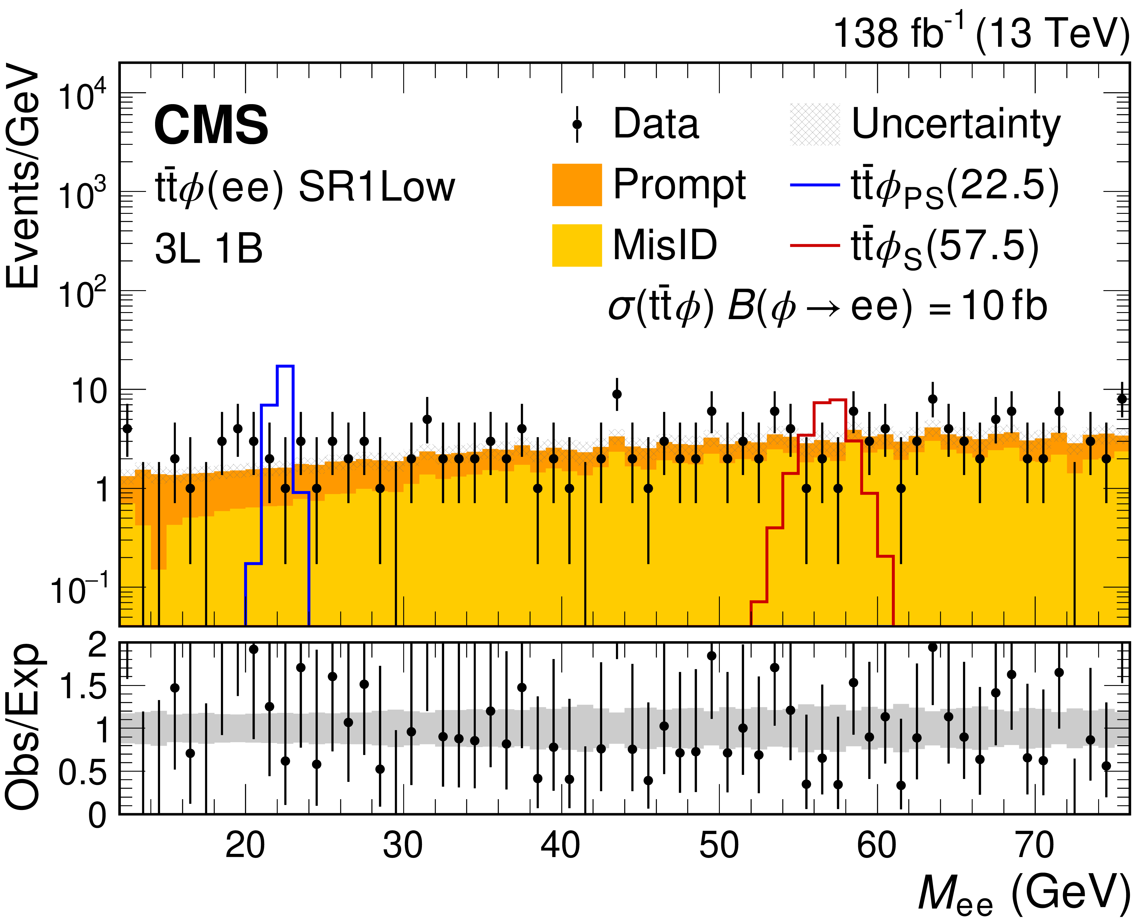
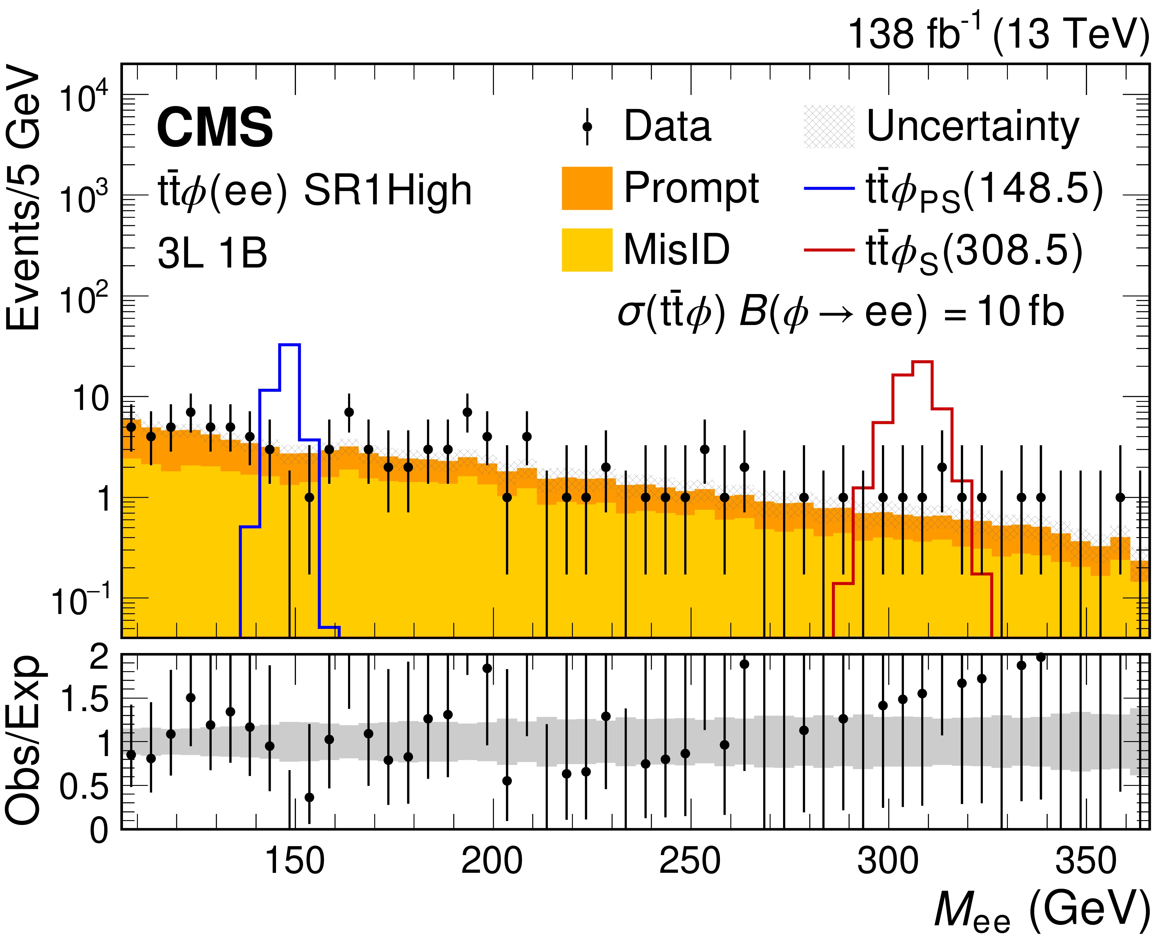
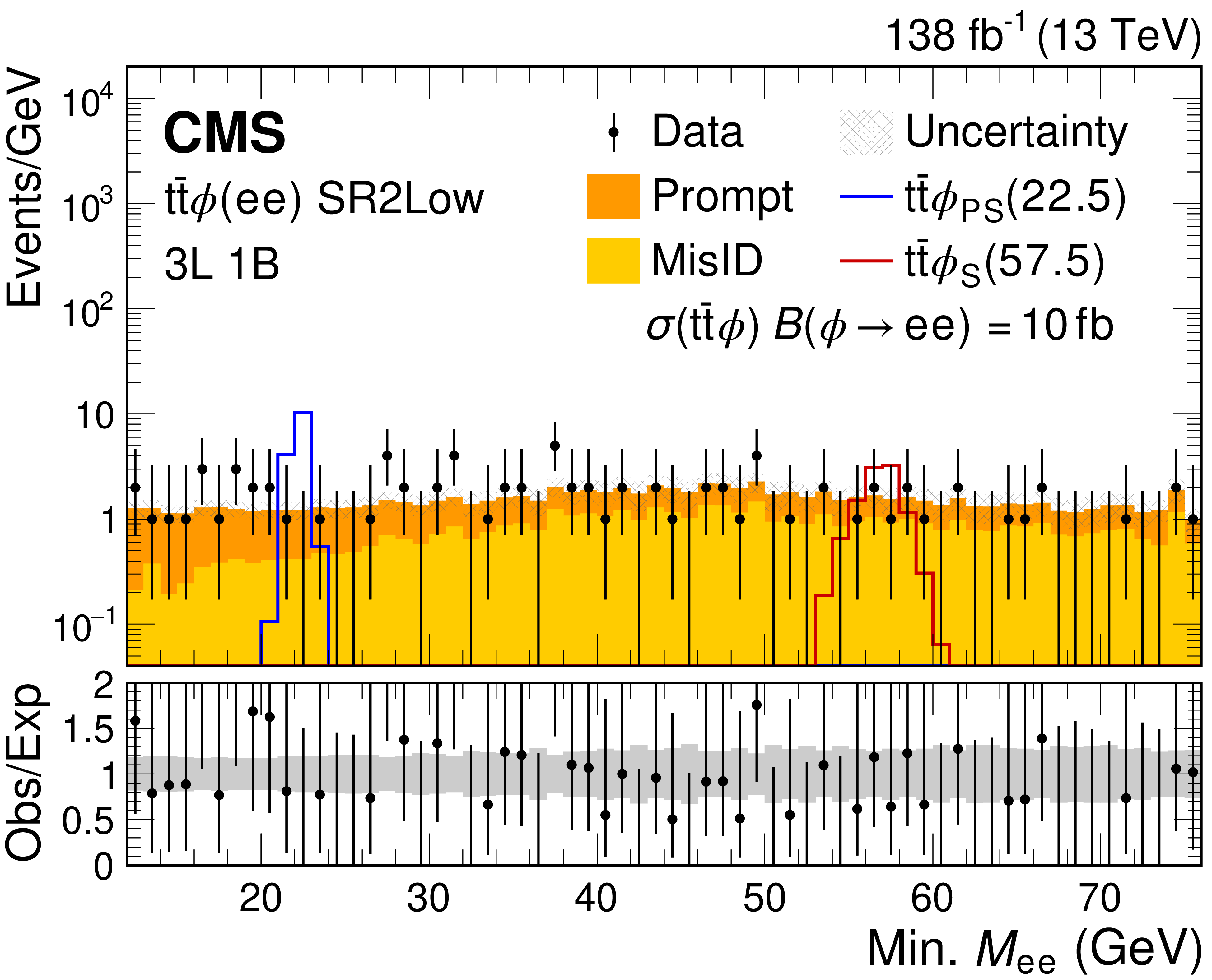
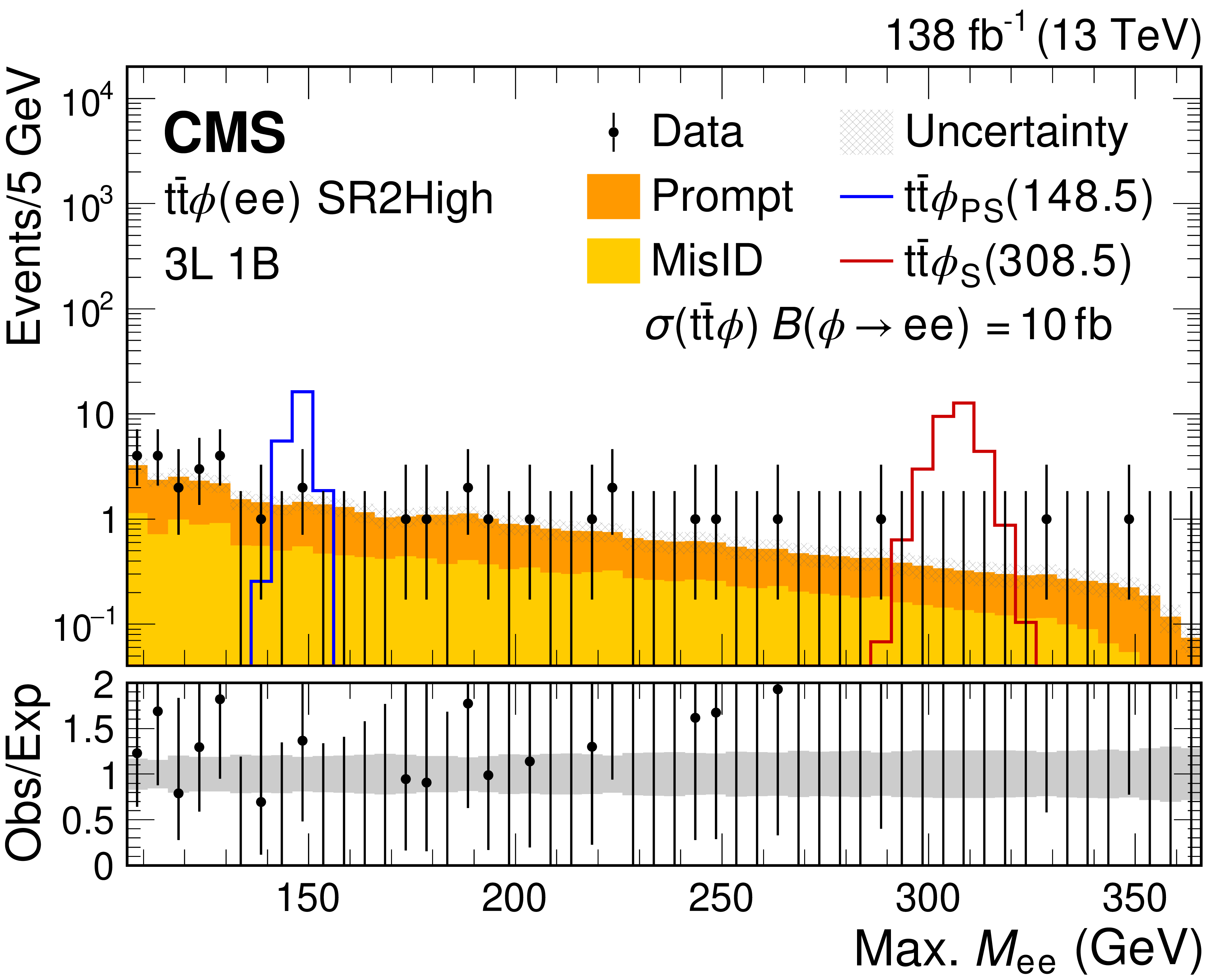
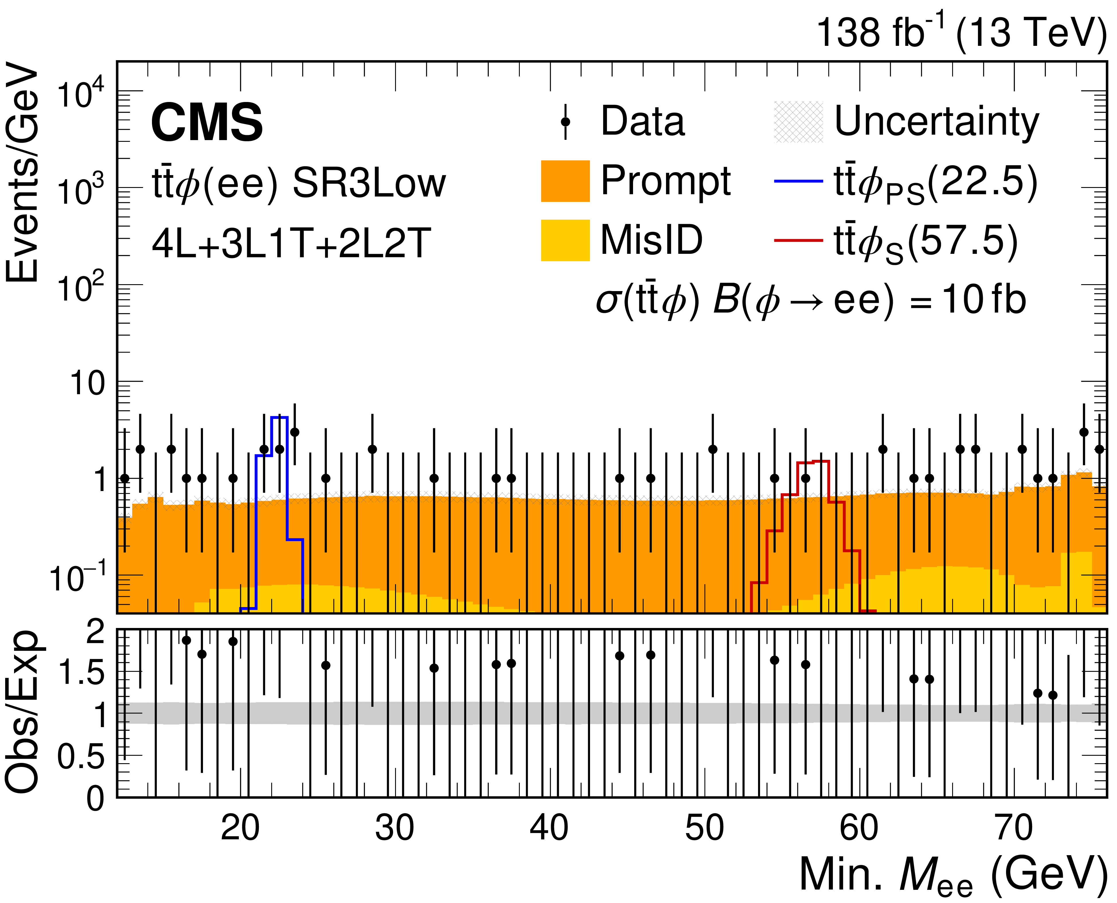
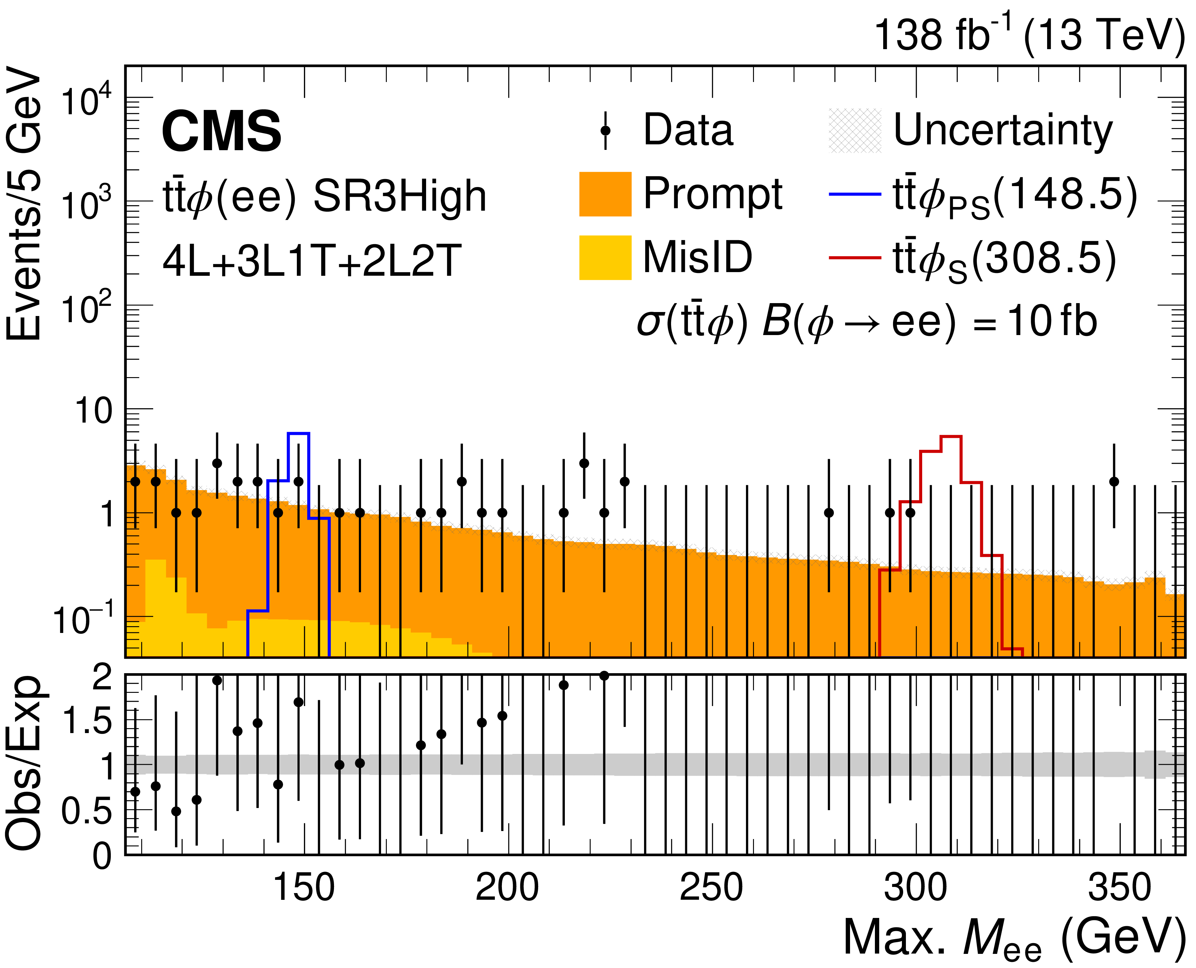
png pdf	Figure 5: Dilepton mass spectra for the $ {{\mathrm{t}\overline{\mathrm{t}}} }{\phi}(\mathrm{e}\mathrm{e}) $ SR1 (upper), SR2 (middle), and SR3 (lower) event selections for the combined 2016-2018 data set. The low (high) mass spectra are shown on the left (right). The lower panel shows the ratio of observed events to the total expected SM background prediction (Obs/Exp), and the gray band represents the sum of statistical and systematic uncertainties in the background prediction. The expected background distributions and the uncertainties are shown after the data is fit under the background-only hypothesis. For illustration, two example signal hypotheses for the production and decay of a scalar and a pseudoscalar $ \phi $ boson are shown, and their masses (in units of GeV) are indicated in the legend. The signals are normalized to the product of the cross section and branching fraction of 10 fb.
png pdf	Figure 5-a: Dilepton low mass spectrum for the $ {{\mathrm{t}\overline{\mathrm{t}}} }{\phi}(\mathrm{e}\mathrm{e}) $ SR1 event selection for the combined 2016-2018 data set. The lower panel shows the ratio of observed events to the total expected SM background prediction (Obs/Exp), and the gray band represents the sum of statistical and systematic uncertainties in the background prediction. The expected background distributions and the uncertainties are shown after the data is fit under the background-only hypothesis. For illustration, two example signal hypotheses for the production and decay of a scalar and a pseudoscalar $ \phi $ boson are shown, and their masses (in units of GeV) are indicated in the legend. The signals are normalized to the product of the cross section and branching fraction of 10 fb.
png pdf	Figure 5-b: Dilepton high mass spectrum for the $ {{\mathrm{t}\overline{\mathrm{t}}} }{\phi}(\mathrm{e}\mathrm{e}) $ SR1 event selection for the combined 2016-2018 data set. The lower panel shows the ratio of observed events to the total expected SM background prediction (Obs/Exp), and the gray band represents the sum of statistical and systematic uncertainties in the background prediction. The expected background distributions and the uncertainties are shown after the data is fit under the background-only hypothesis. For illustration, two example signal hypotheses for the production and decay of a scalar and a pseudoscalar $ \phi $ boson are shown, and their masses (in units of GeV) are indicated in the legend. The signals are normalized to the product of the cross section and branching fraction of 10 fb.
png pdf	Figure 5-c: Dilepton low mass spectrum for the $ {{\mathrm{t}\overline{\mathrm{t}}} }{\phi}(\mathrm{e}\mathrm{e}) $ SR2 event selection for the combined 2016-2018 data set. The lower panel shows the ratio of observed events to the total expected SM background prediction (Obs/Exp), and the gray band represents the sum of statistical and systematic uncertainties in the background prediction. The expected background distributions and the uncertainties are shown after the data is fit under the background-only hypothesis. For illustration, two example signal hypotheses for the production and decay of a scalar and a pseudoscalar $ \phi $ boson are shown, and their masses (in units of GeV) are indicated in the legend. The signals are normalized to the product of the cross section and branching fraction of 10 fb.
png pdf	Figure 5-d: Dilepton high mass spectrum for the $ {{\mathrm{t}\overline{\mathrm{t}}} }{\phi}(\mathrm{e}\mathrm{e}) $ SR2 event selection for the combined 2016-2018 data set. The lower panel shows the ratio of observed events to the total expected SM background prediction (Obs/Exp), and the gray band represents the sum of statistical and systematic uncertainties in the background prediction. The expected background distributions and the uncertainties are shown after the data is fit under the background-only hypothesis. For illustration, two example signal hypotheses for the production and decay of a scalar and a pseudoscalar $ \phi $ boson are shown, and their masses (in units of GeV) are indicated in the legend. The signals are normalized to the product of the cross section and branching fraction of 10 fb.
png pdf	Figure 5-e: Dilepton low mass spectrum for the $ {{\mathrm{t}\overline{\mathrm{t}}} }{\phi}(\mathrm{e}\mathrm{e}) $ SR3 event selection for the combined 2016-2018 data set. The lower panel shows the ratio of observed events to the total expected SM background prediction (Obs/Exp), and the gray band represents the sum of statistical and systematic uncertainties in the background prediction. The expected background distributions and the uncertainties are shown after the data is fit under the background-only hypothesis. For illustration, two example signal hypotheses for the production and decay of a scalar and a pseudoscalar $ \phi $ boson are shown, and their masses (in units of GeV) are indicated in the legend. The signals are normalized to the product of the cross section and branching fraction of 10 fb.
png pdf	Figure 5-f: Dilepton high mass spectrum for the $ {{\mathrm{t}\overline{\mathrm{t}}} }{\phi}(\mathrm{e}\mathrm{e}) $ SR3 event selection for the combined 2016-2018 data set. The lower panel shows the ratio of observed events to the total expected SM background prediction (Obs/Exp), and the gray band represents the sum of statistical and systematic uncertainties in the background prediction. The expected background distributions and the uncertainties are shown after the data is fit under the background-only hypothesis. For illustration, two example signal hypotheses for the production and decay of a scalar and a pseudoscalar $ \phi $ boson are shown, and their masses (in units of GeV) are indicated in the legend. The signals are normalized to the product of the cross section and branching fraction of 10 fb.
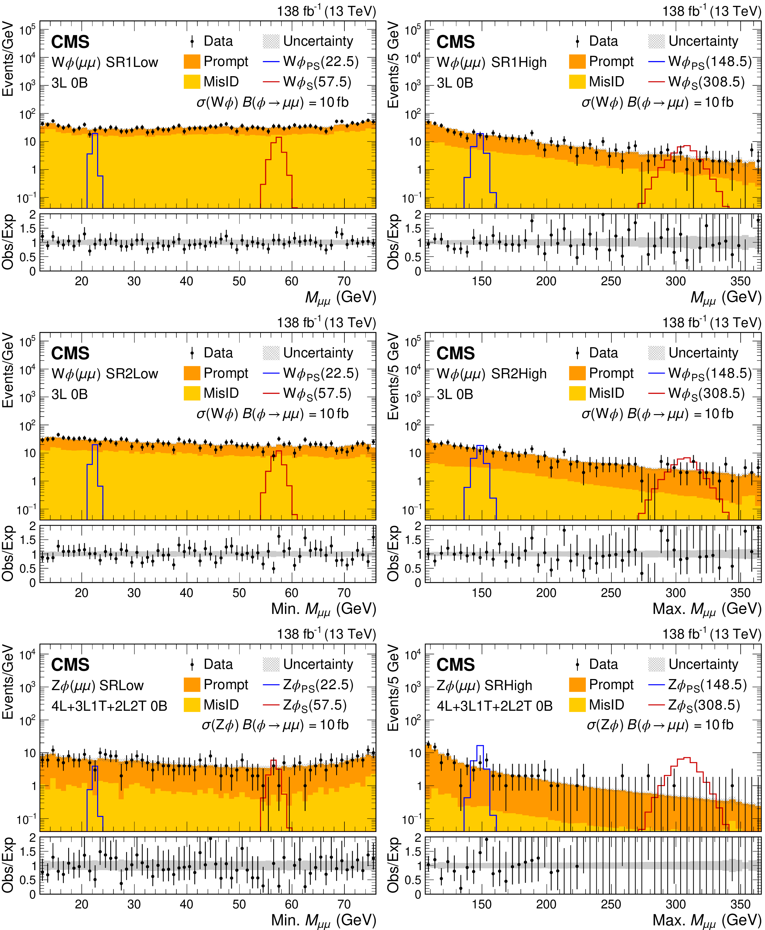
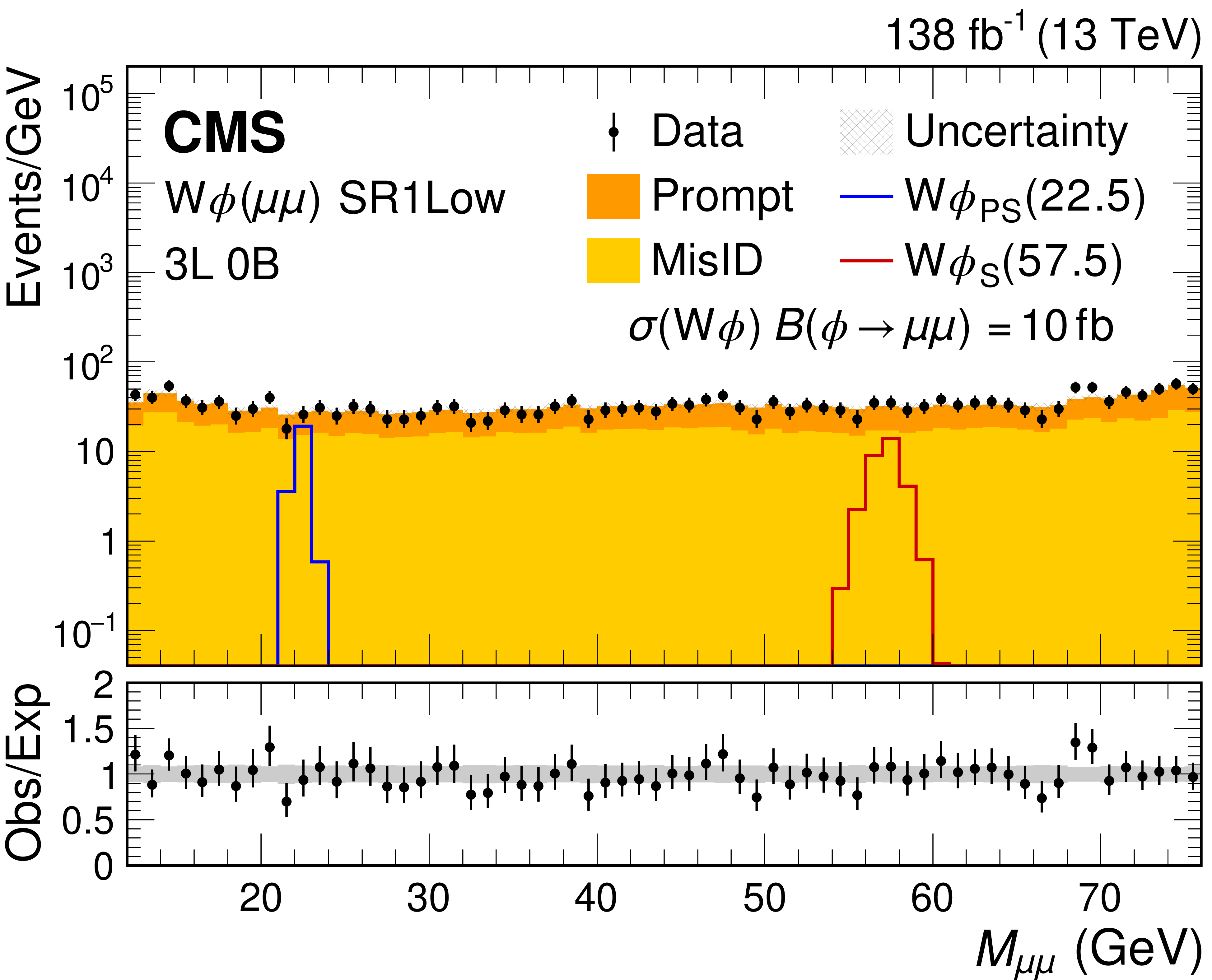
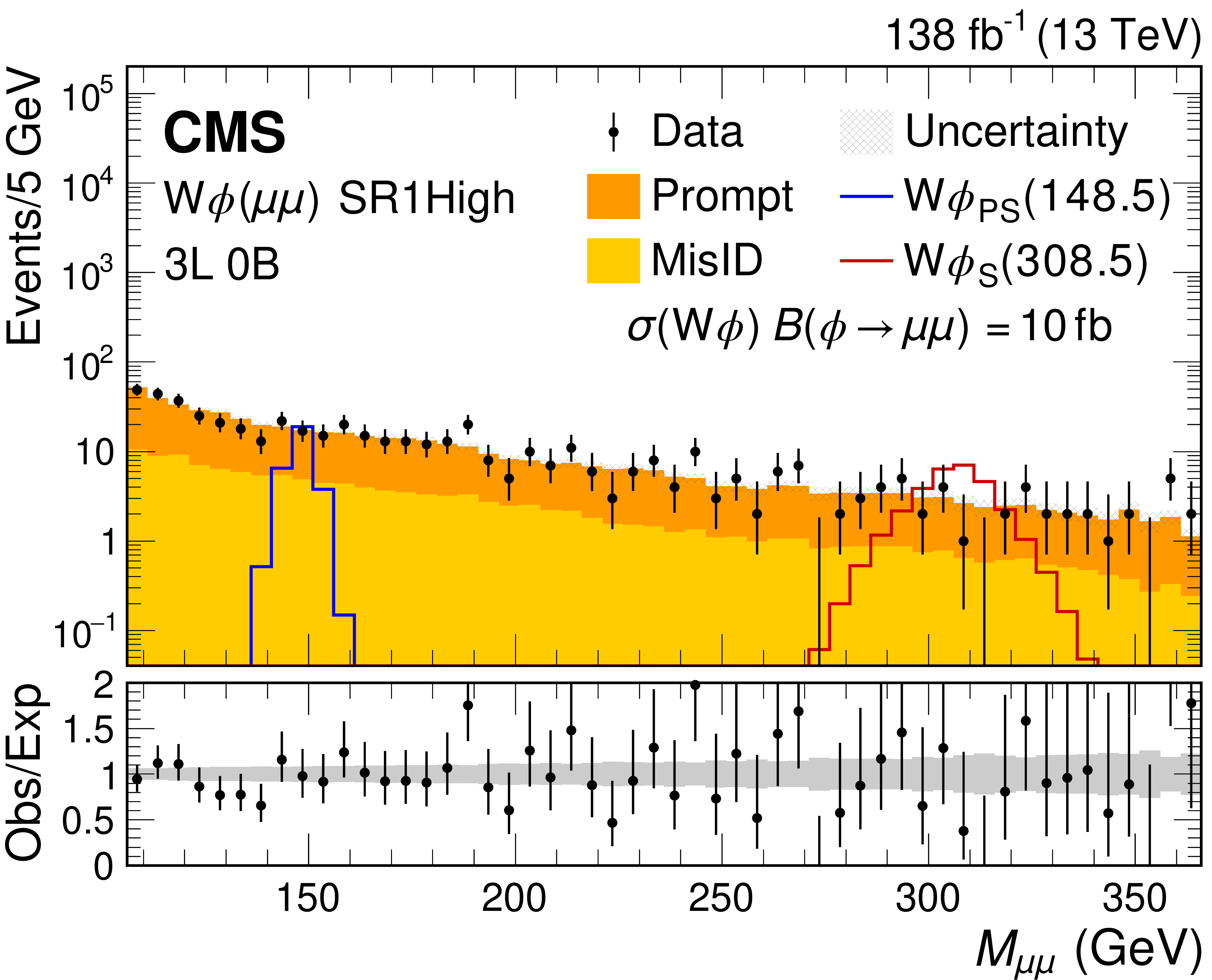
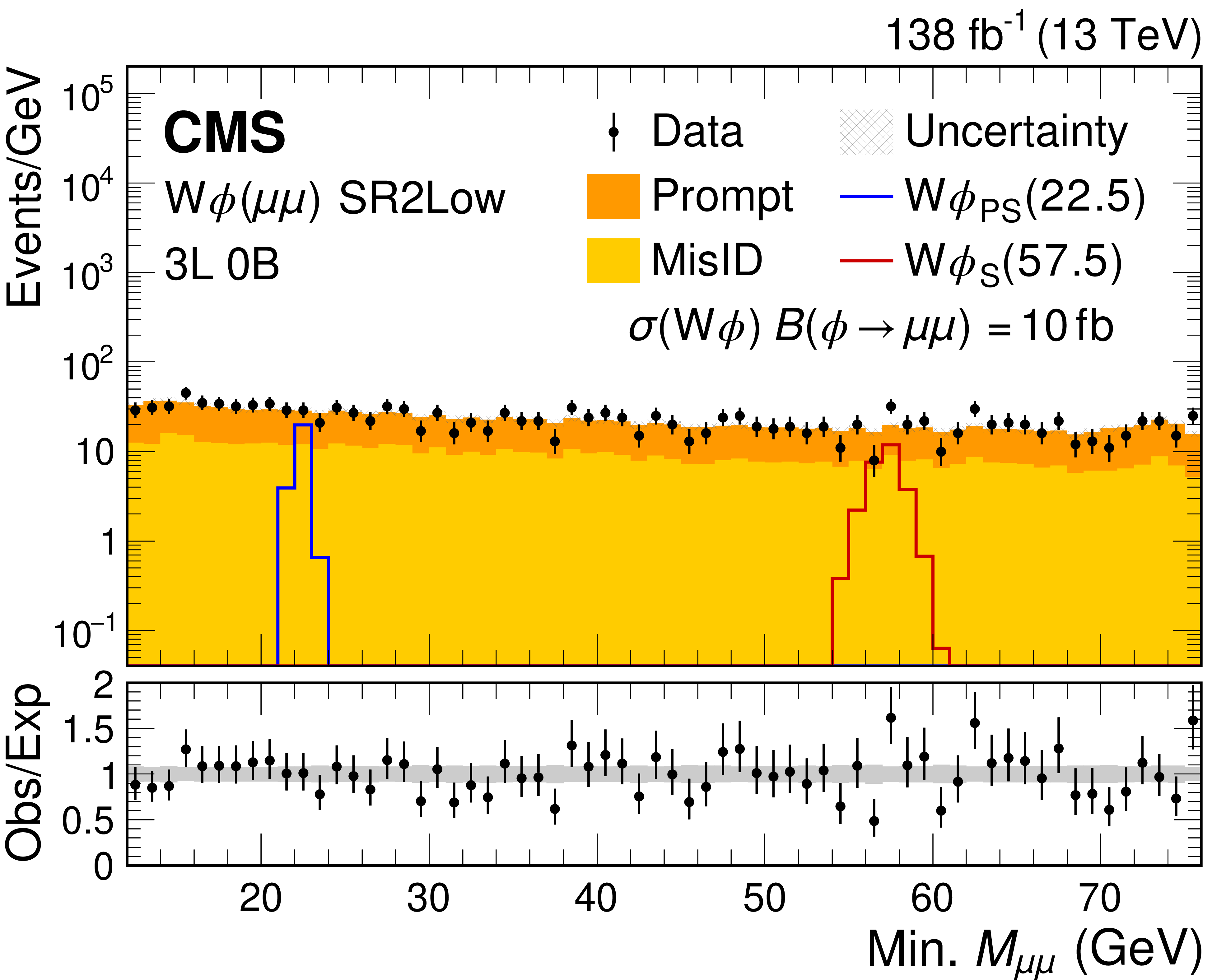
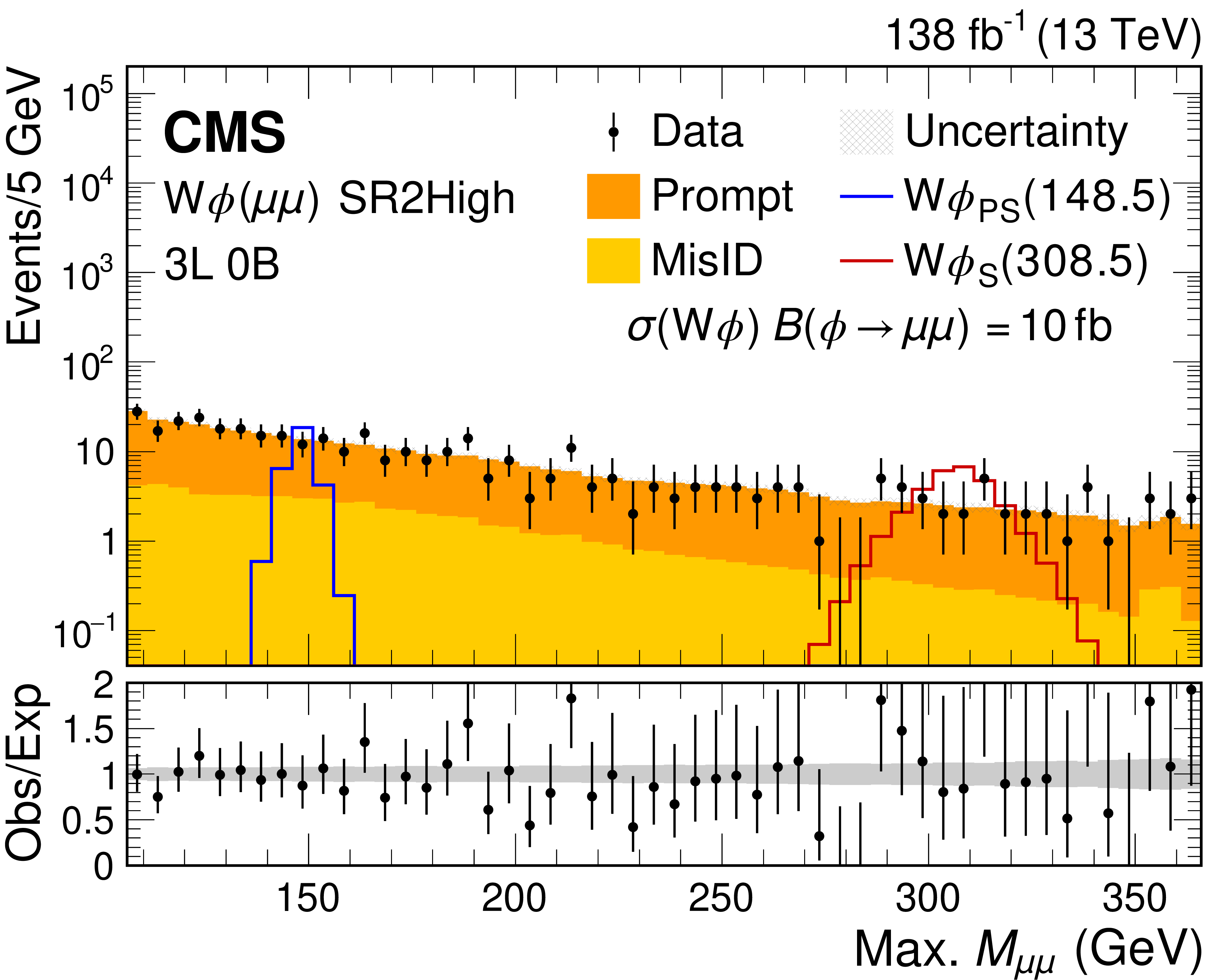
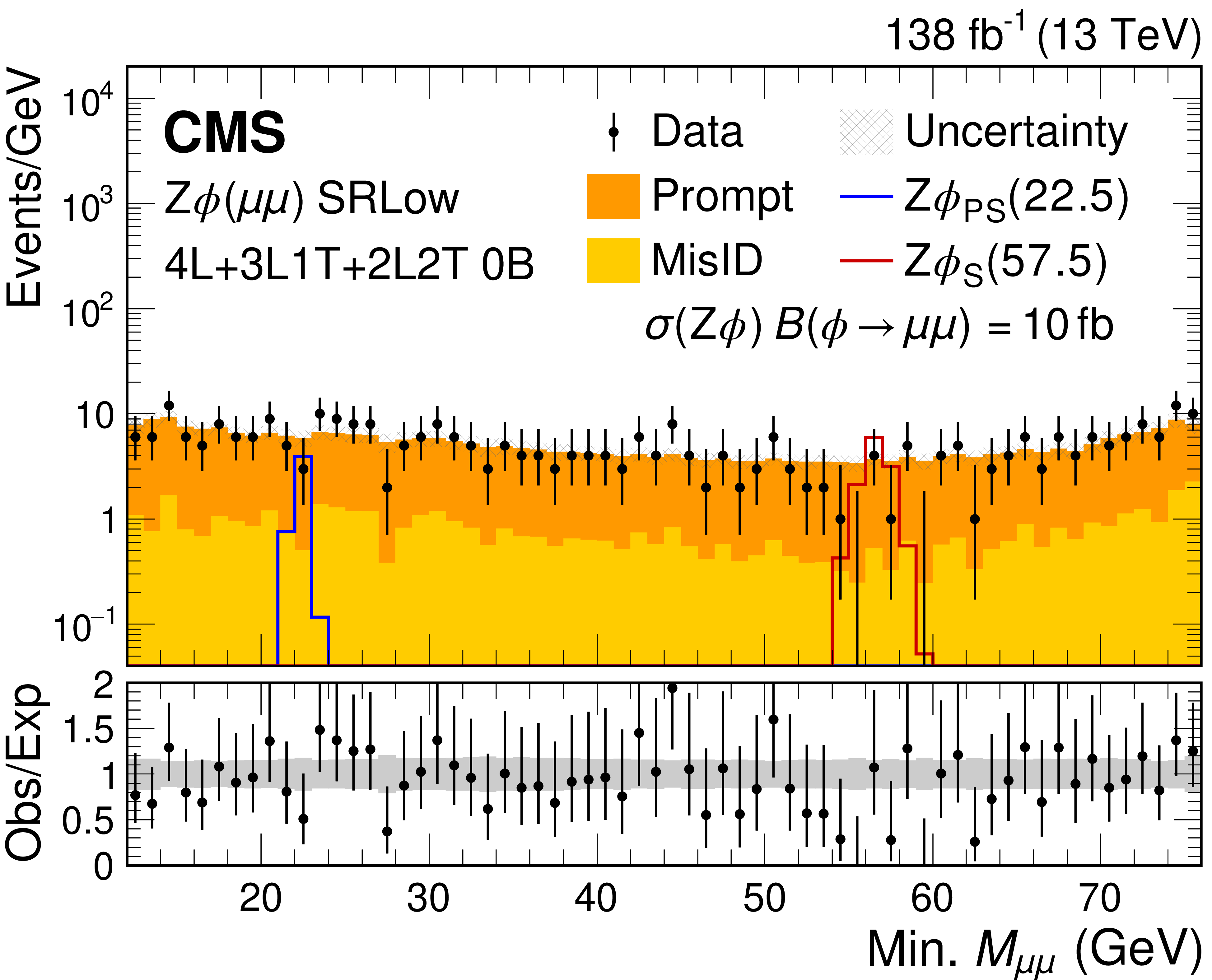
png pdf	Figure 6: Dilepton mass spectra for the $ {\mathrm{W}}{\phi}(\mu\mu) $ SR1 (upper), SR2 (middle), and $ {\mathrm{Z}}{\phi}(\mu\mu) $ SR (lower) event selections for the combined 2016-2018 data set. The low (high) mass spectra are shown on the left (right). The lower panel shows the ratio of observed events to the total expected SM background prediction (Obs/Exp), and the gray band represents the sum of statistical and systematic uncertainties in the background prediction. The expected background distributions and the uncertainties are shown after the data is fit under the background-only hypothesis. For illustration, two example signal hypotheses for the production and decay of a scalar and a pseudoscalar $ \phi $ boson are shown, and their masses (in units of GeV) are indicated in the legend. The signals are normalized to the product of the cross section and branching fraction of 10 fb.
png pdf	Figure 6-a: Dilepton low mass spectrum for the $ {\mathrm{W}}{\phi}(\mu\mu) $ SR1 event selection for the combined 2016-2018 data set. The lower panel shows the ratio of observed events to the total expected SM background prediction (Obs/Exp), and the gray band represents the sum of statistical and systematic uncertainties in the background prediction. The expected background distributions and the uncertainties are shown after the data is fit under the background-only hypothesis. For illustration, two example signal hypotheses for the production and decay of a scalar and a pseudoscalar $ \phi $ boson are shown, and their masses (in units of GeV) are indicated in the legend. The signals are normalized to the product of the cross section and branching fraction of 10 fb.
png pdf	Figure 6-b: Dilepton high mass spectrum for the $ {\mathrm{W}}{\phi}(\mu\mu) $ SR1 event selection for the combined 2016-2018 data set. The lower panel shows the ratio of observed events to the total expected SM background prediction (Obs/Exp), and the gray band represents the sum of statistical and systematic uncertainties in the background prediction. The expected background distributions and the uncertainties are shown after the data is fit under the background-only hypothesis. For illustration, two example signal hypotheses for the production and decay of a scalar and a pseudoscalar $ \phi $ boson are shown, and their masses (in units of GeV) are indicated in the legend. The signals are normalized to the product of the cross section and branching fraction of 10 fb.
png pdf	Figure 6-c: Dilepton low mass spectrum for the $ {\mathrm{W}}{\phi}(\mu\mu) $ SR2 event selection for the combined 2016-2018 data set. The lower panel shows the ratio of observed events to the total expected SM background prediction (Obs/Exp), and the gray band represents the sum of statistical and systematic uncertainties in the background prediction. The expected background distributions and the uncertainties are shown after the data is fit under the background-only hypothesis. For illustration, two example signal hypotheses for the production and decay of a scalar and a pseudoscalar $ \phi $ boson are shown, and their masses (in units of GeV) are indicated in the legend. The signals are normalized to the product of the cross section and branching fraction of 10 fb.
png pdf	Figure 6-d: Dilepton high mass spectrum for the $ {\mathrm{W}}{\phi}(\mu\mu) $ SR2 event selection for the combined 2016-2018 data set. The lower panel shows the ratio of observed events to the total expected SM background prediction (Obs/Exp), and the gray band represents the sum of statistical and systematic uncertainties in the background prediction. The expected background distributions and the uncertainties are shown after the data is fit under the background-only hypothesis. For illustration, two example signal hypotheses for the production and decay of a scalar and a pseudoscalar $ \phi $ boson are shown, and their masses (in units of GeV) are indicated in the legend. The signals are normalized to the product of the cross section and branching fraction of 10 fb.
png pdf	Figure 6-e: Dilepton low mass spectrum for the $ {\mathrm{Z}}{\phi}(\mu\mu) $ SR event selection for the combined 2016-2018 data set. The lower panel shows the ratio of observed events to the total expected SM background prediction (Obs/Exp), and the gray band represents the sum of statistical and systematic uncertainties in the background prediction. The expected background distributions and the uncertainties are shown after the data is fit under the background-only hypothesis. For illustration, two example signal hypotheses for the production and decay of a scalar and a pseudoscalar $ \phi $ boson are shown, and their masses (in units of GeV) are indicated in the legend. The signals are normalized to the product of the cross section and branching fraction of 10 fb.
png pdf	Figure 6-f: Dilepton high mass spectrum for the $ {\mathrm{Z}}{\phi}(\mu\mu) $ SR event selection for the combined 2016-2018 data set. The lower panel shows the ratio of observed events to the total expected SM background prediction (Obs/Exp), and the gray band represents the sum of statistical and systematic uncertainties in the background prediction. The expected background distributions and the uncertainties are shown after the data is fit under the background-only hypothesis. For illustration, two example signal hypotheses for the production and decay of a scalar and a pseudoscalar $ \phi $ boson are shown, and their masses (in units of GeV) are indicated in the legend. The signals are normalized to the product of the cross section and branching fraction of 10 fb.
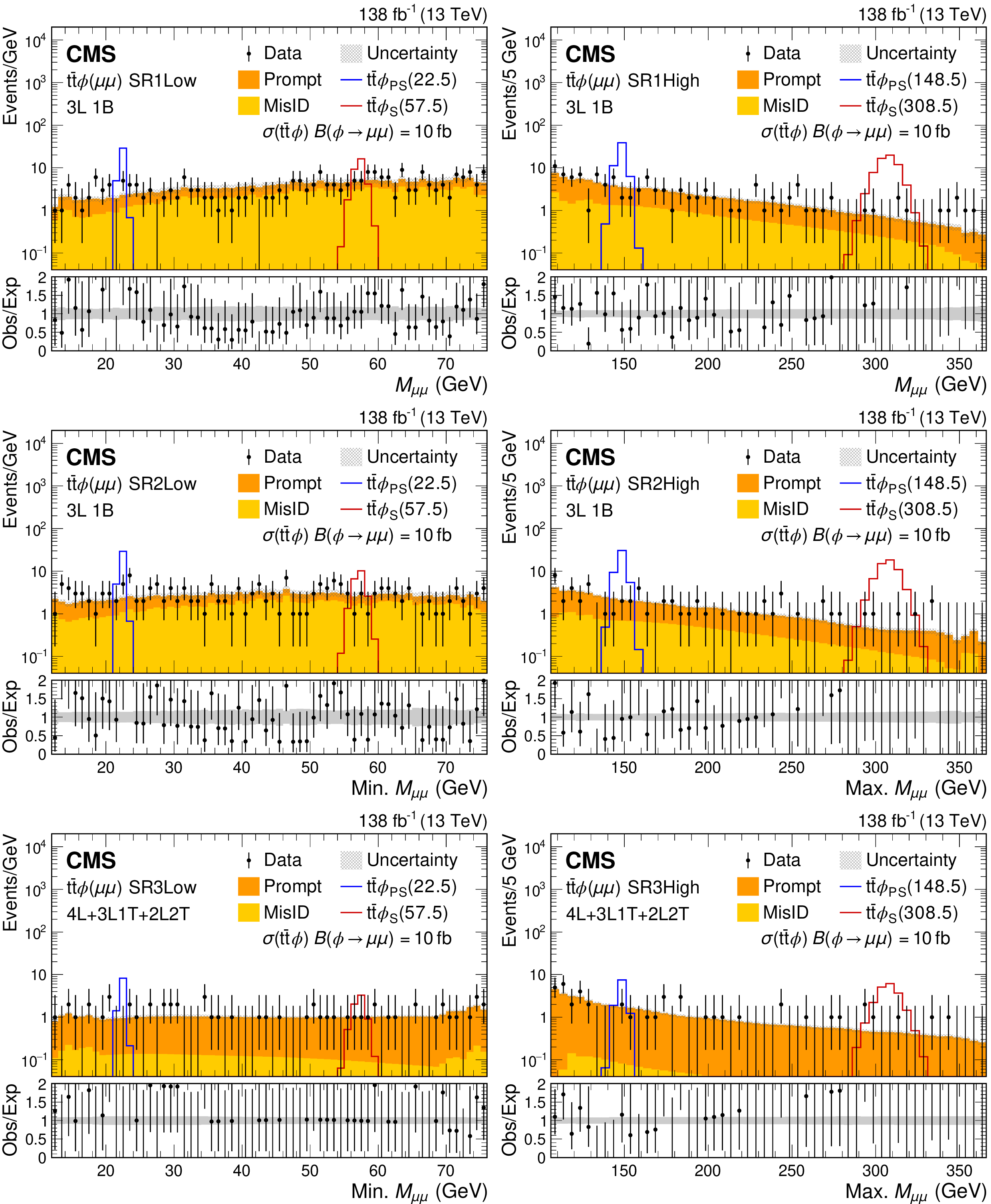
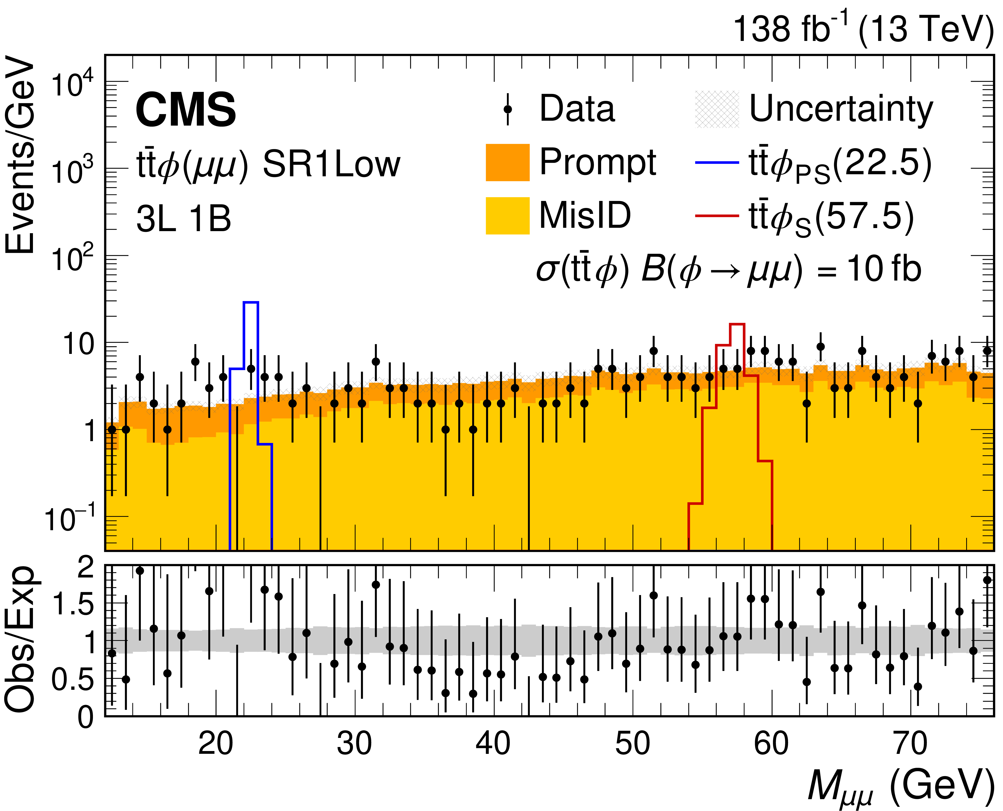
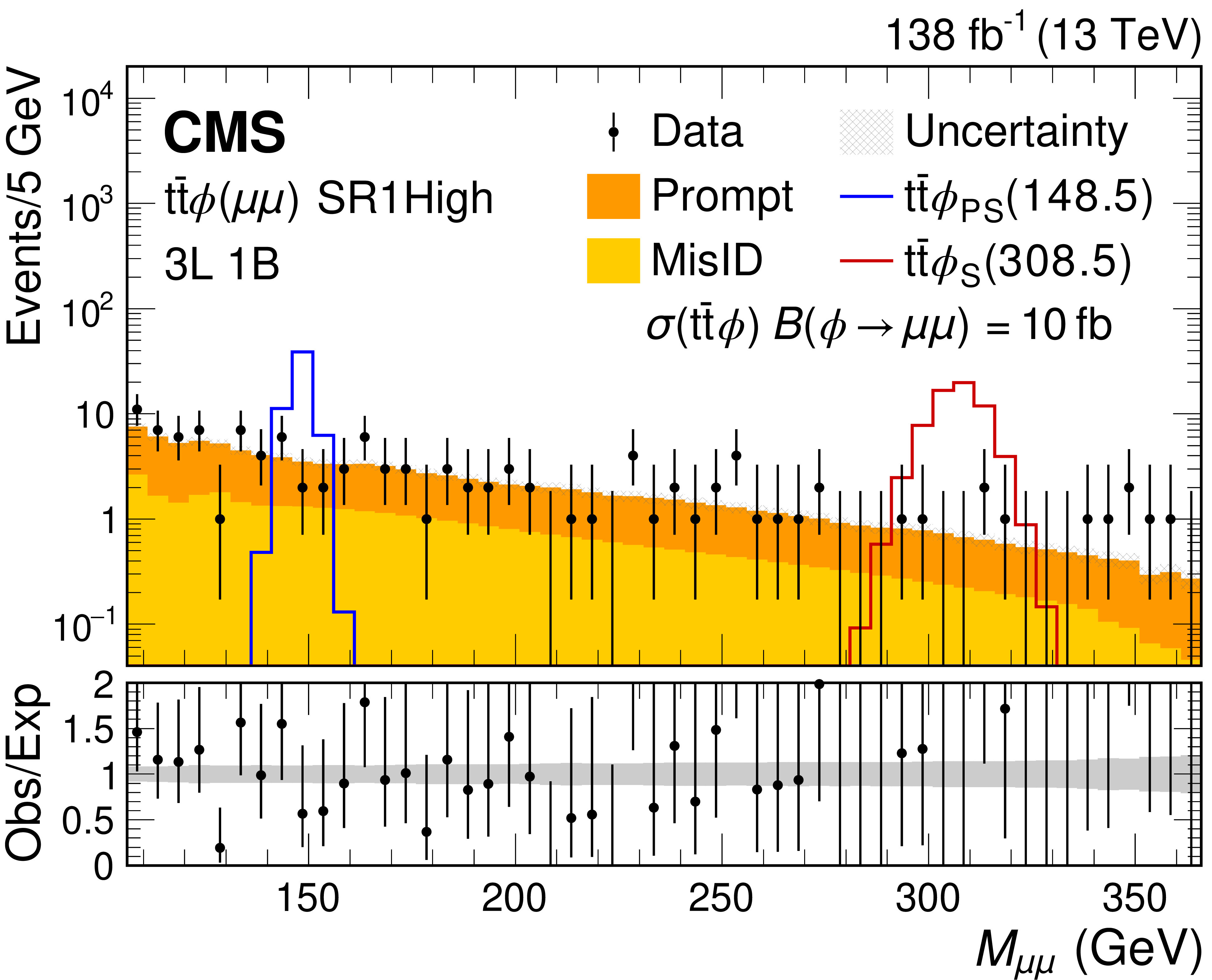
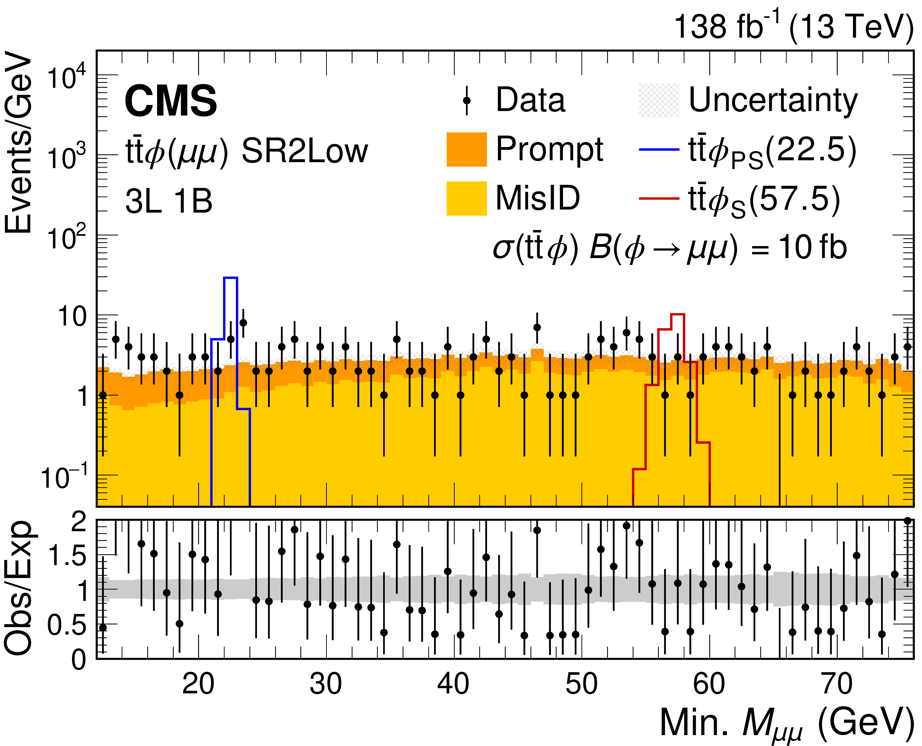
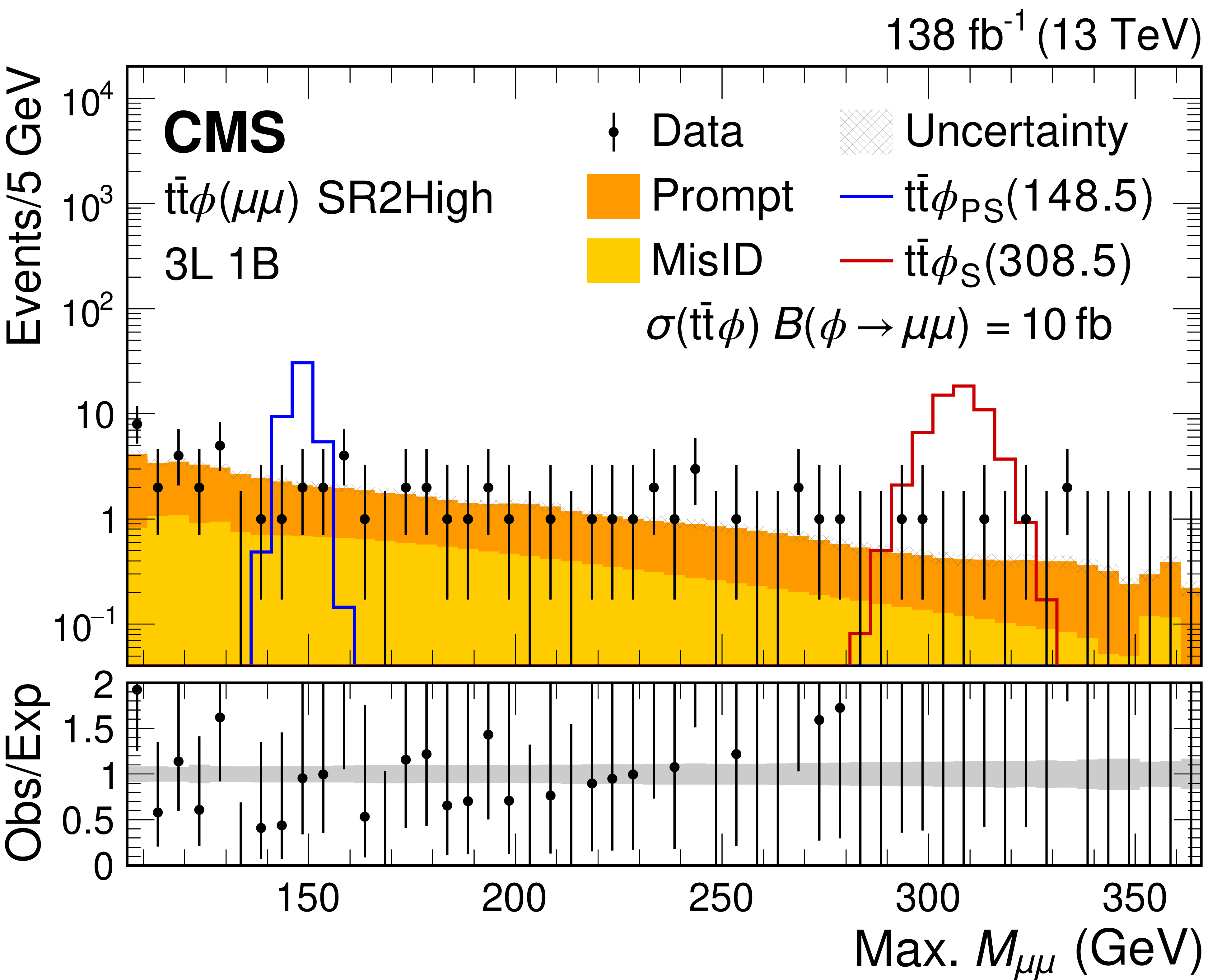
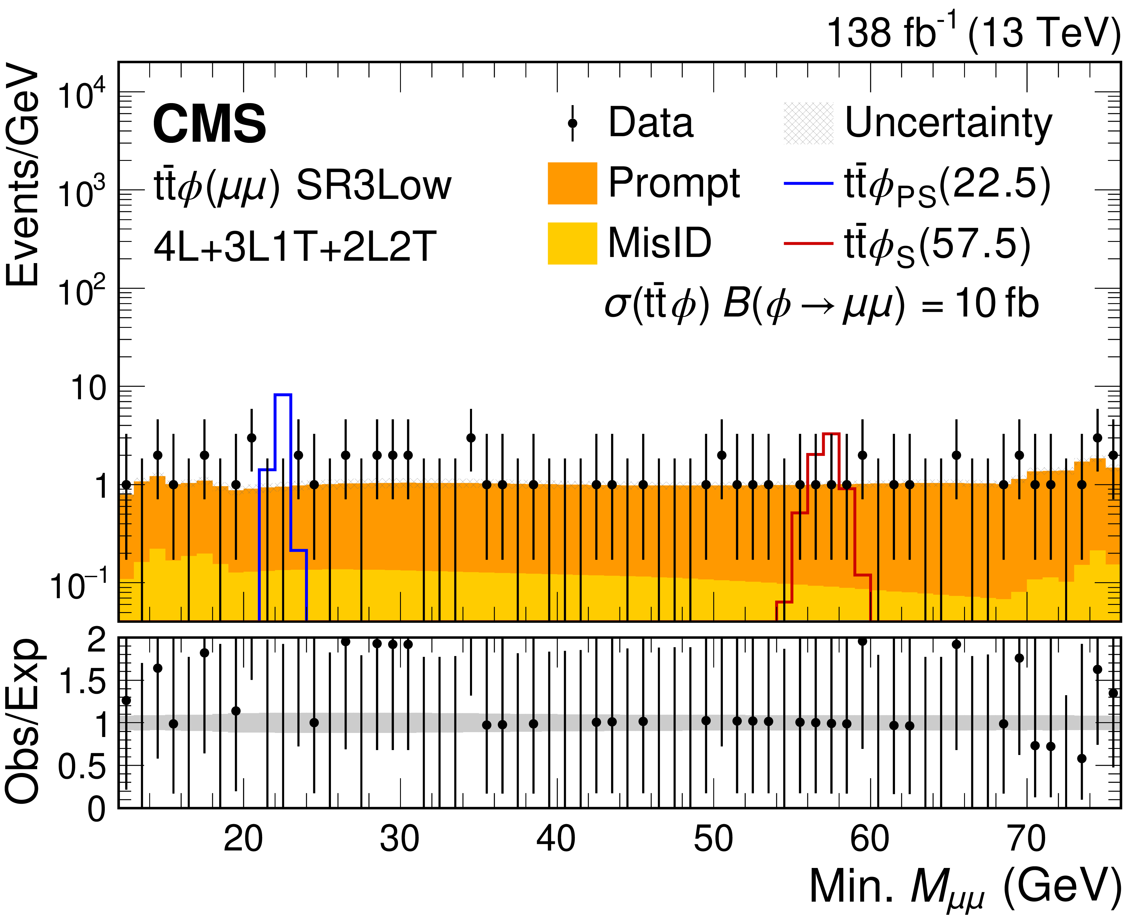
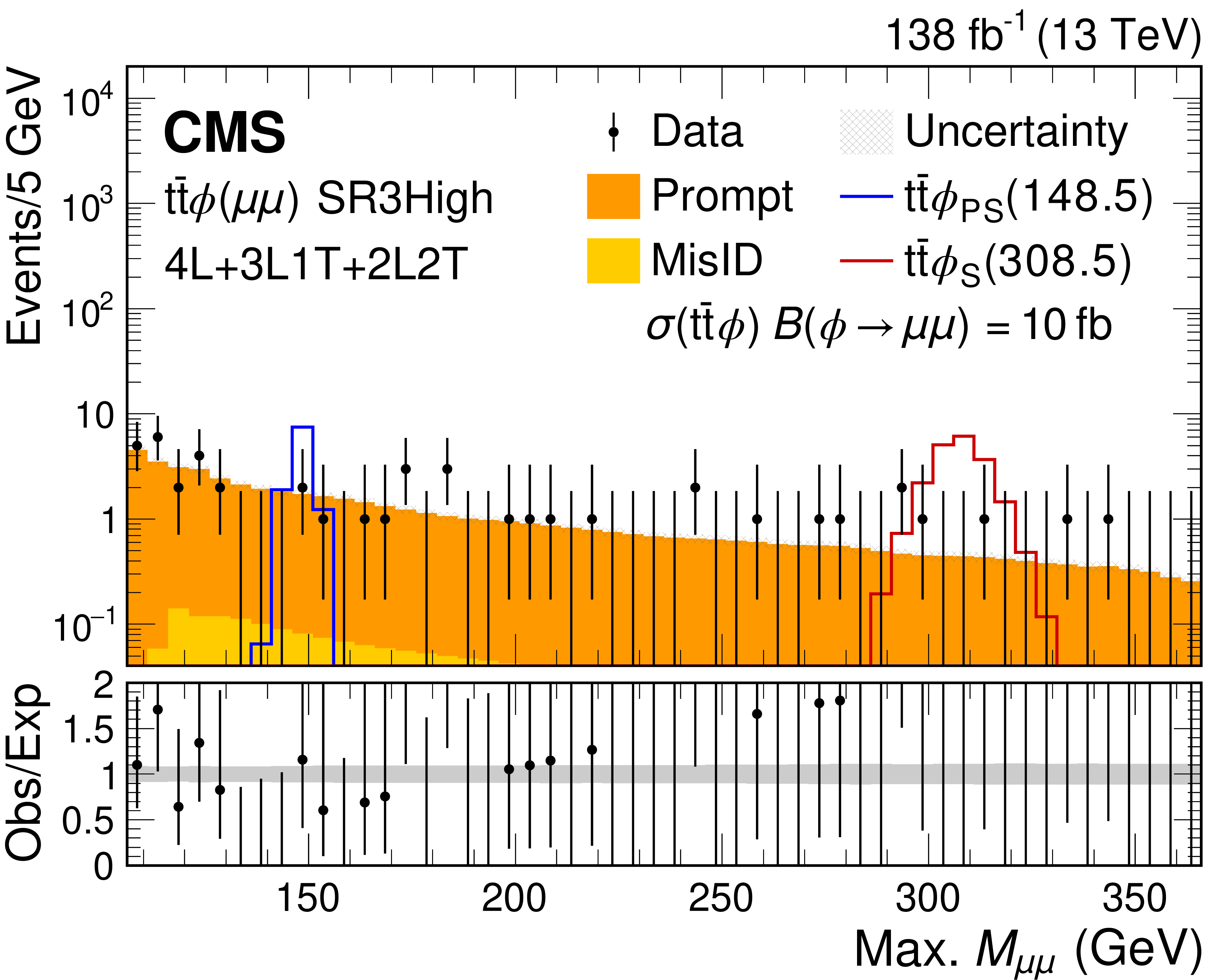
png pdf	Figure 7: Dilepton mass spectra for the $ {{\mathrm{t}\overline{\mathrm{t}}} }{\phi}(\mu\mu) $ SR1 (upper), SR2 (middle), and SR3 (lower) event selections for the combined 2016-2018 data set. The low (high) mass spectra are shown on the left (right). The lower panel shows the ratio of observed events to the total expected SM background prediction (Obs/Exp), and the gray band represents the sum of statistical and systematic uncertainties in the background prediction. The expected background distributions and the uncertainties are shown after the data is fit under the background-only hypothesis. For illustration, two example signal hypotheses for the production and decay of a scalar and a pseudoscalar $ \phi $ boson are shown, and their masses (in units of GeV) are indicated in the legend. The signals are normalized to the product of the cross section and branching fraction of 10 fb.
png pdf	Figure 7-a: Dilepton low mass spectrum for the $ {{\mathrm{t}\overline{\mathrm{t}}} }{\phi}(\mu\mu) $ SR1 event selection for the combined 2016-2018 data set. The lower panel shows the ratio of observed events to the total expected SM background prediction (Obs/Exp), and the gray band represents the sum of statistical and systematic uncertainties in the background prediction. The expected background distributions and the uncertainties are shown after the data is fit under the background-only hypothesis. For illustration, two example signal hypotheses for the production and decay of a scalar and a pseudoscalar $ \phi $ boson are shown, and their masses (in units of GeV) are indicated in the legend. The signals are normalized to the product of the cross section and branching fraction of 10 fb.
png pdf	Figure 7-b: Dilepton high mass spectrum for the $ {{\mathrm{t}\overline{\mathrm{t}}} }{\phi}(\mu\mu) $ SR1 event selection for the combined 2016-2018 data set. The lower panel shows the ratio of observed events to the total expected SM background prediction (Obs/Exp), and the gray band represents the sum of statistical and systematic uncertainties in the background prediction. The expected background distributions and the uncertainties are shown after the data is fit under the background-only hypothesis. For illustration, two example signal hypotheses for the production and decay of a scalar and a pseudoscalar $ \phi $ boson are shown, and their masses (in units of GeV) are indicated in the legend. The signals are normalized to the product of the cross section and branching fraction of 10 fb.
png pdf	Figure 7-c: Dilepton low mass spectrum for the $ {{\mathrm{t}\overline{\mathrm{t}}} }{\phi}(\mu\mu) $ SR2 event selection for the combined 2016-2018 data set. The lower panel shows the ratio of observed events to the total expected SM background prediction (Obs/Exp), and the gray band represents the sum of statistical and systematic uncertainties in the background prediction. The expected background distributions and the uncertainties are shown after the data is fit under the background-only hypothesis. For illustration, two example signal hypotheses for the production and decay of a scalar and a pseudoscalar $ \phi $ boson are shown, and their masses (in units of GeV) are indicated in the legend. The signals are normalized to the product of the cross section and branching fraction of 10 fb.
png pdf	Figure 7-d: Dilepton high mass spectrum for the $ {{\mathrm{t}\overline{\mathrm{t}}} }{\phi}(\mu\mu) $ SR2 event selection for the combined 2016-2018 data set. The lower panel shows the ratio of observed events to the total expected SM background prediction (Obs/Exp), and the gray band represents the sum of statistical and systematic uncertainties in the background prediction. The expected background distributions and the uncertainties are shown after the data is fit under the background-only hypothesis. For illustration, two example signal hypotheses for the production and decay of a scalar and a pseudoscalar $ \phi $ boson are shown, and their masses (in units of GeV) are indicated in the legend. The signals are normalized to the product of the cross section and branching fraction of 10 fb.
png pdf	Figure 7-e: Dilepton low mass spectrum for the $ {{\mathrm{t}\overline{\mathrm{t}}} }{\phi}(\mu\mu) $ SR3 event selection for the combined 2016-2018 data set. The lower panel shows the ratio of observed events to the total expected SM background prediction (Obs/Exp), and the gray band represents the sum of statistical and systematic uncertainties in the background prediction. The expected background distributions and the uncertainties are shown after the data is fit under the background-only hypothesis. For illustration, two example signal hypotheses for the production and decay of a scalar and a pseudoscalar $ \phi $ boson are shown, and their masses (in units of GeV) are indicated in the legend. The signals are normalized to the product of the cross section and branching fraction of 10 fb.
png pdf	Figure 7-f: Dilepton high mass spectrum for the $ {{\mathrm{t}\overline{\mathrm{t}}} }{\phi}(\mu\mu) $ SR3 event selection for the combined 2016-2018 data set. The lower panel shows the ratio of observed events to the total expected SM background prediction (Obs/Exp), and the gray band represents the sum of statistical and systematic uncertainties in the background prediction. The expected background distributions and the uncertainties are shown after the data is fit under the background-only hypothesis. For illustration, two example signal hypotheses for the production and decay of a scalar and a pseudoscalar $ \phi $ boson are shown, and their masses (in units of GeV) are indicated in the legend. The signals are normalized to the product of the cross section and branching fraction of 10 fb.
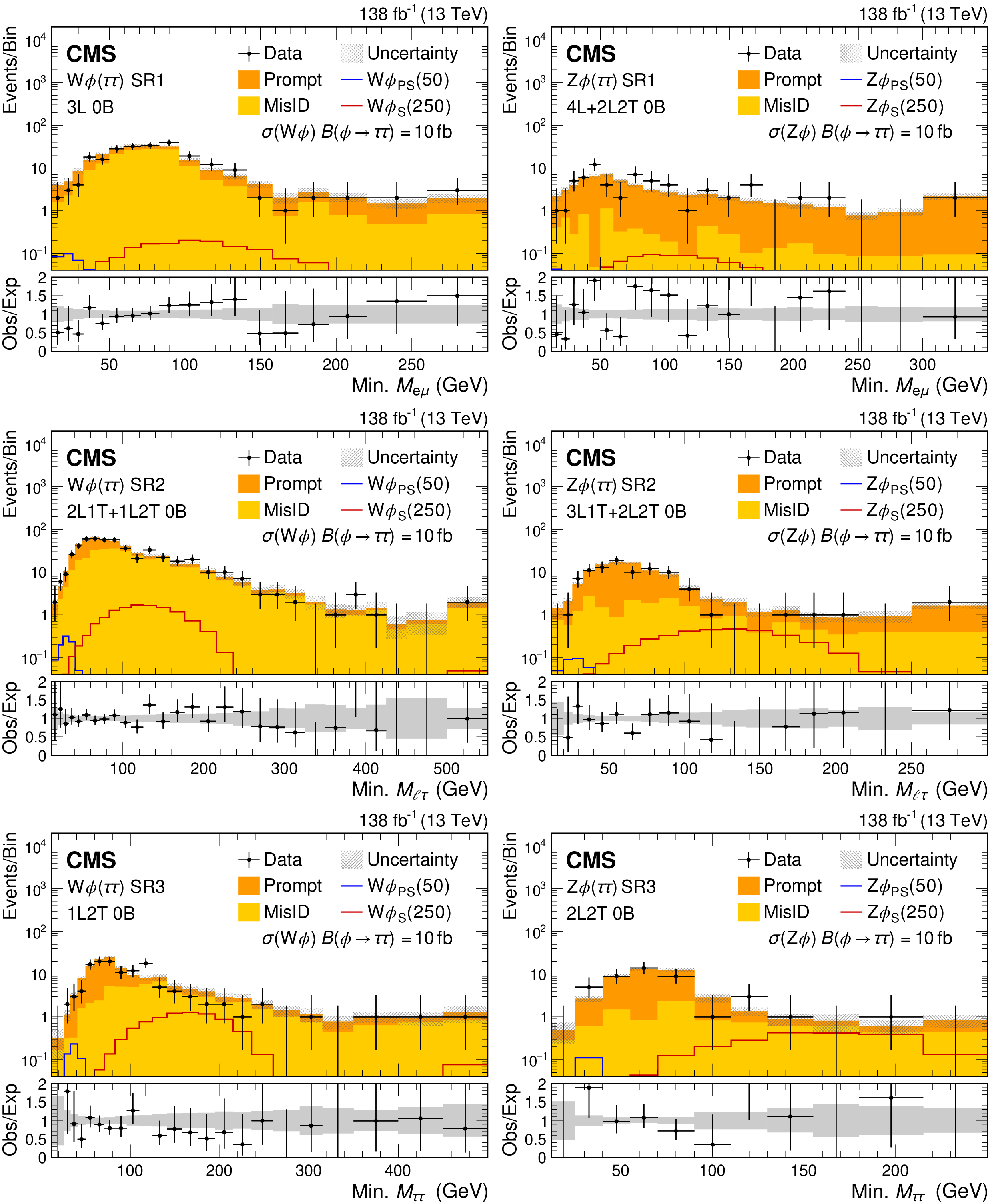
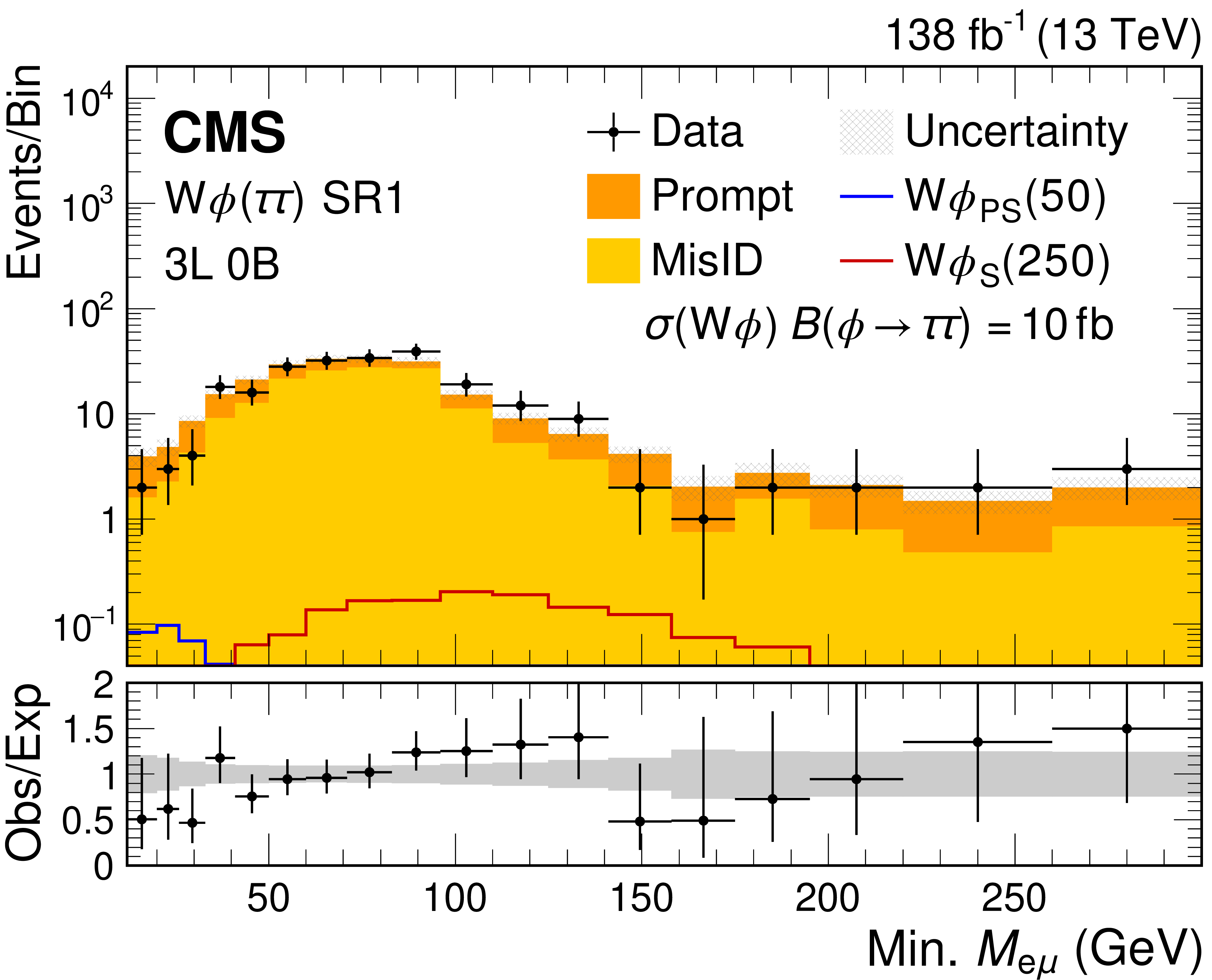
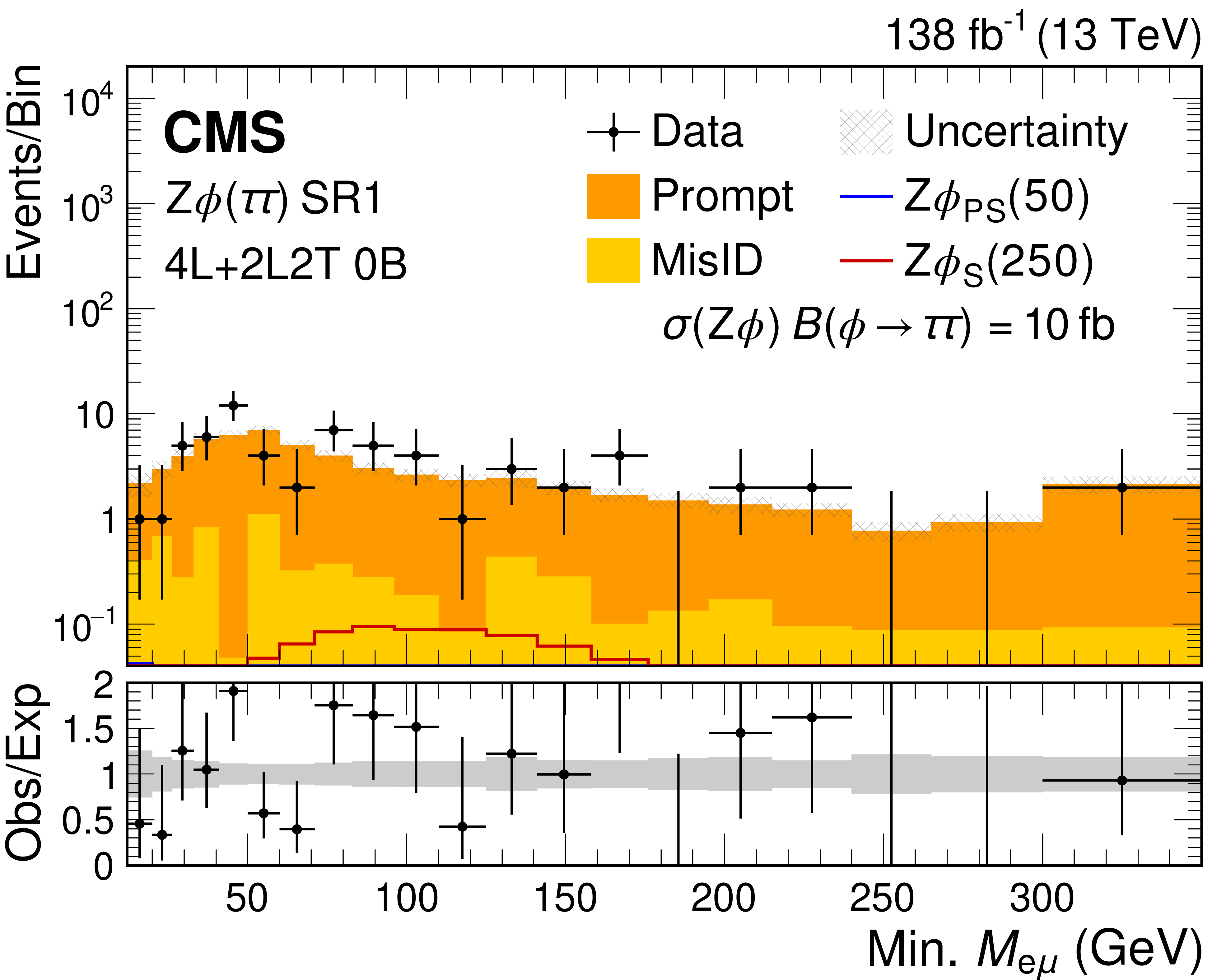
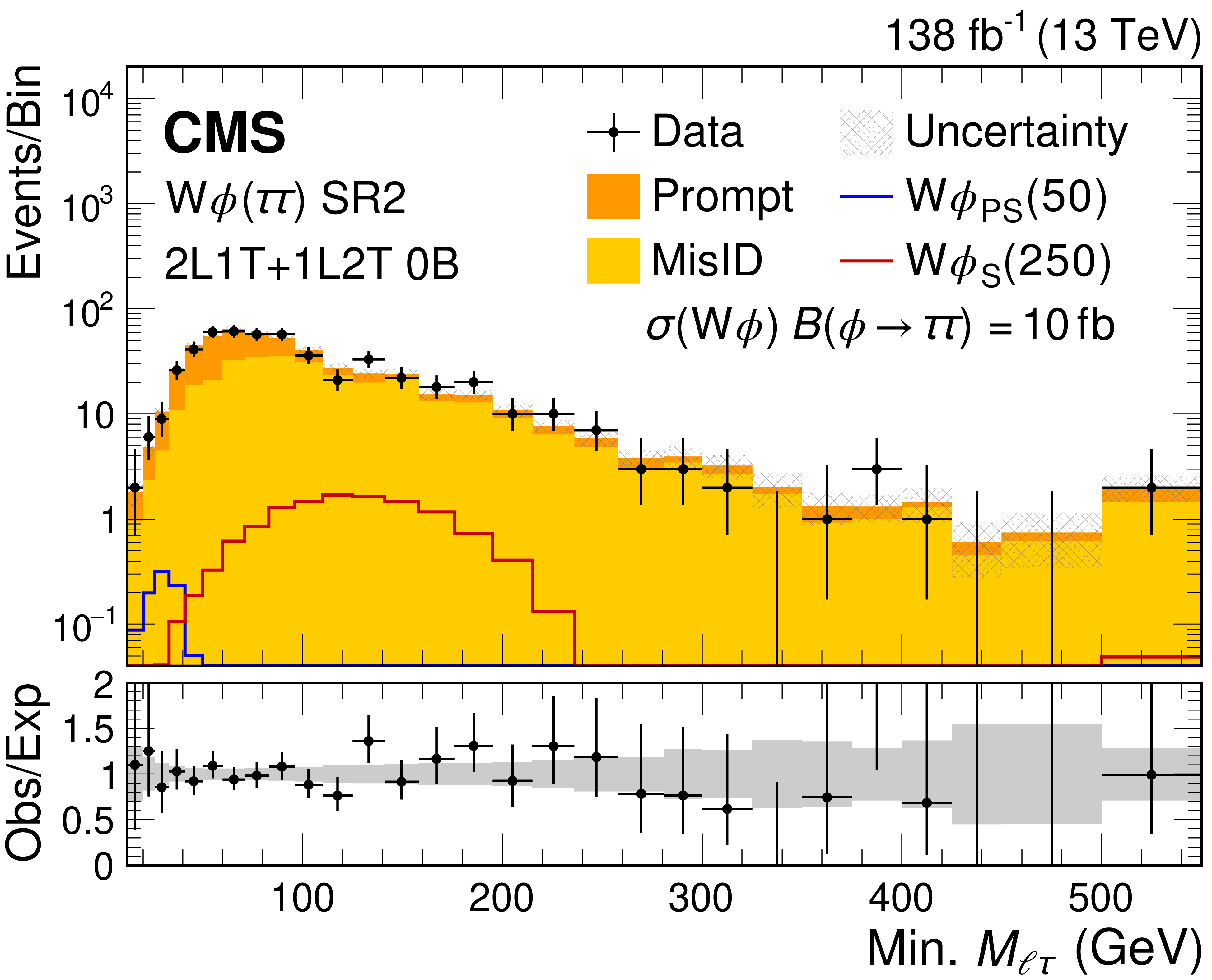
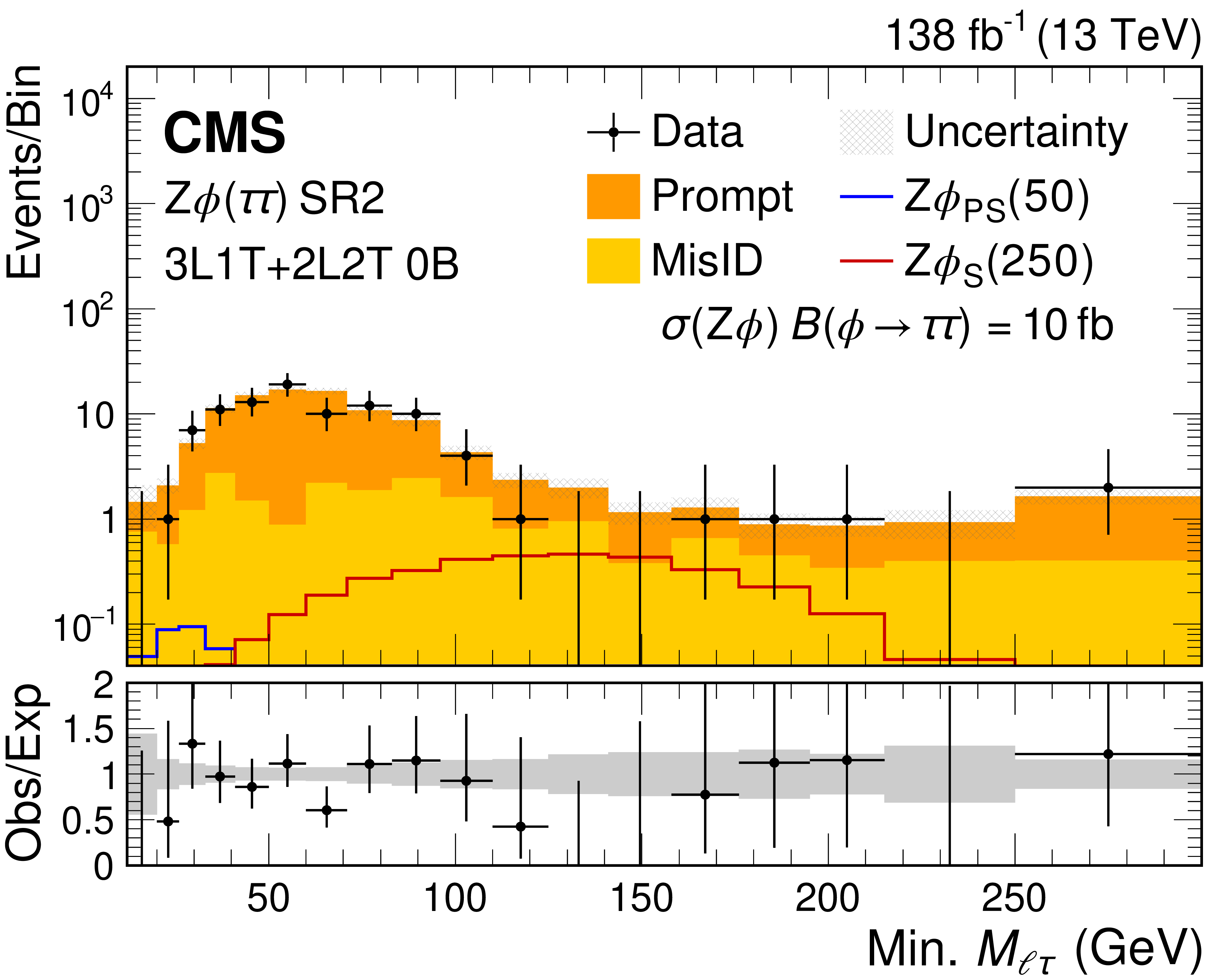
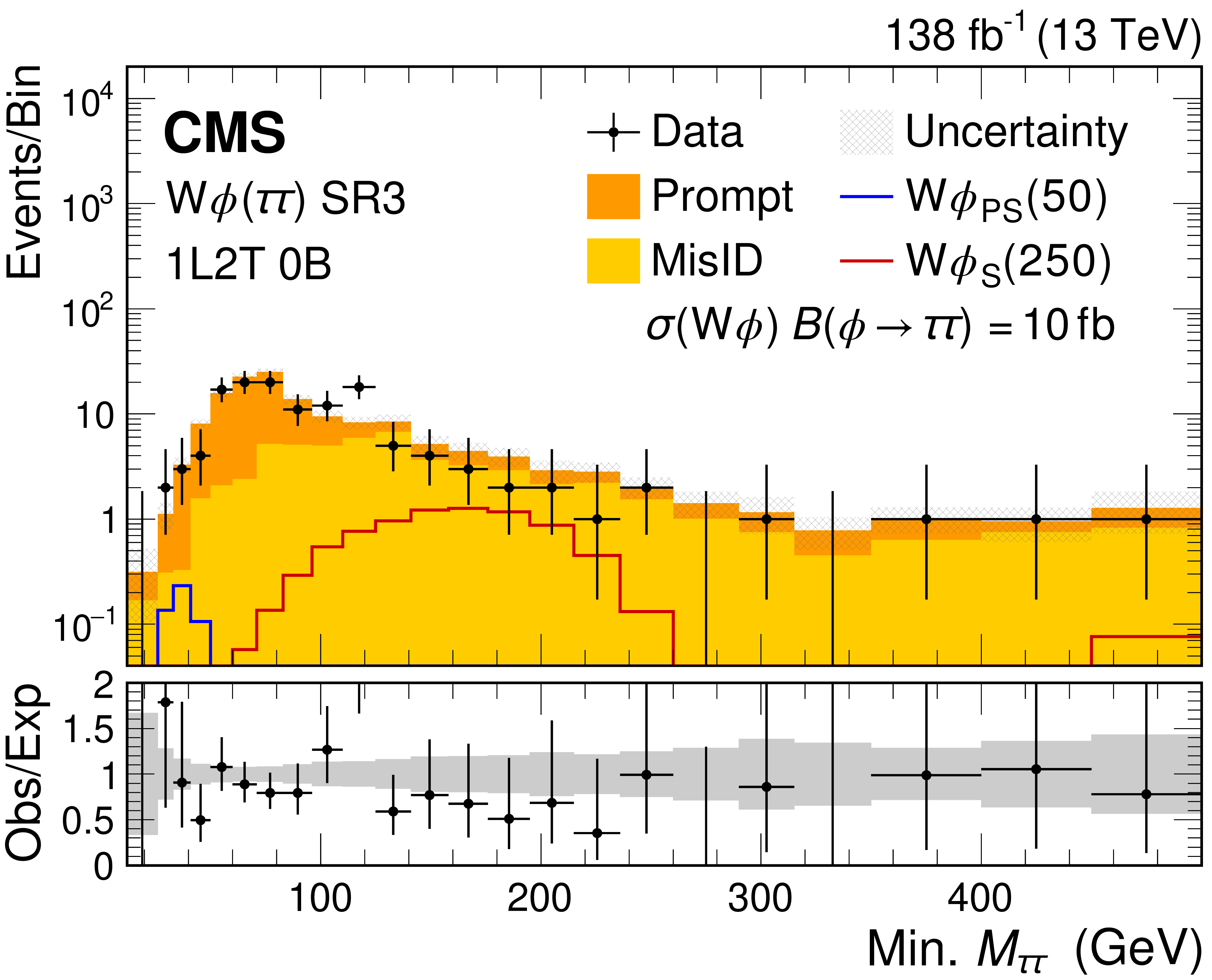
png pdf	Figure 8: Dilepton mass spectra for the $ {\mathrm{W}}{\phi}(\tau\tau) $ SR (left) and $ {\mathrm{Z}}{\phi}(\tau\tau) $ SR (right) event selections for the combined 2016-2018 data set. The lower panel shows the ratio of observed events to the total expected SM background prediction (Obs/Exp), and the gray band represents the sum of statistical and systematic uncertainties in the background prediction. The rightmost bins contain the overflow events in each distribution. The expected background distributions and the uncertainties are shown after the data is fit under the background-only hypothesis. For illustration, two example signal hypotheses for the production and decay of a scalar and a pseudoscalar $ \phi $ boson are shown, and their masses (in units of GeV) are indicated in the legend. The signals are normalized to the product of the cross section and branching fraction of 10 fb.
png pdf	Figure 8-a: Dilepton mass spectra for the $ {\mathrm{W}}{\phi}(\tau\tau) $ SR1 event selection for the combined 2016-2018 data set. The lower panel shows the ratio of observed events to the total expected SM background prediction (Obs/Exp), and the gray band represents the sum of statistical and systematic uncertainties in the background prediction. The rightmost bins contain the overflow events in each distribution. The expected background distributions and the uncertainties are shown after the data is fit under the background-only hypothesis. For illustration, two example signal hypotheses for the production and decay of a scalar and a pseudoscalar $ \phi $ boson are shown, and their masses (in units of GeV) are indicated in the legend. The signals are normalized to the product of the cross section and branching fraction of 10 fb.
png pdf	Figure 8-b: Dilepton mass spectra for the $ {\mathrm{Z}}{\phi}(\tau\tau) $ SR1 event selection for the combined 2016-2018 data set. The lower panel shows the ratio of observed events to the total expected SM background prediction (Obs/Exp), and the gray band represents the sum of statistical and systematic uncertainties in the background prediction. The rightmost bins contain the overflow events in each distribution. The expected background distributions and the uncertainties are shown after the data is fit under the background-only hypothesis. For illustration, two example signal hypotheses for the production and decay of a scalar and a pseudoscalar $ \phi $ boson are shown, and their masses (in units of GeV) are indicated in the legend. The signals are normalized to the product of the cross section and branching fraction of 10 fb.
png pdf	Figure 8-c: Dilepton mass spectra for the $ {\mathrm{W}}{\phi}(\tau\tau) $ SR2 event selection for the combined 2016-2018 data set. The lower panel shows the ratio of observed events to the total expected SM background prediction (Obs/Exp), and the gray band represents the sum of statistical and systematic uncertainties in the background prediction. The rightmost bins contain the overflow events in each distribution. The expected background distributions and the uncertainties are shown after the data is fit under the background-only hypothesis. For illustration, two example signal hypotheses for the production and decay of a scalar and a pseudoscalar $ \phi $ boson are shown, and their masses (in units of GeV) are indicated in the legend. The signals are normalized to the product of the cross section and branching fraction of 10 fb.
png pdf	Figure 8-d: Dilepton mass spectra for the $ {\mathrm{Z}}{\phi}(\tau\tau) $ SR2 event selection for the combined 2016-2018 data set. The lower panel shows the ratio of observed events to the total expected SM background prediction (Obs/Exp), and the gray band represents the sum of statistical and systematic uncertainties in the background prediction. The rightmost bins contain the overflow events in each distribution. The expected background distributions and the uncertainties are shown after the data is fit under the background-only hypothesis. For illustration, two example signal hypotheses for the production and decay of a scalar and a pseudoscalar $ \phi $ boson are shown, and their masses (in units of GeV) are indicated in the legend. The signals are normalized to the product of the cross section and branching fraction of 10 fb.
png pdf	Figure 8-e: Dilepton mass spectra for the $ {\mathrm{W}}{\phi}(\tau\tau) $ SR3 event selection for the combined 2016-2018 data set. The lower panel shows the ratio of observed events to the total expected SM background prediction (Obs/Exp), and the gray band represents the sum of statistical and systematic uncertainties in the background prediction. The rightmost bins contain the overflow events in each distribution. The expected background distributions and the uncertainties are shown after the data is fit under the background-only hypothesis. For illustration, two example signal hypotheses for the production and decay of a scalar and a pseudoscalar $ \phi $ boson are shown, and their masses (in units of GeV) are indicated in the legend. The signals are normalized to the product of the cross section and branching fraction of 10 fb.
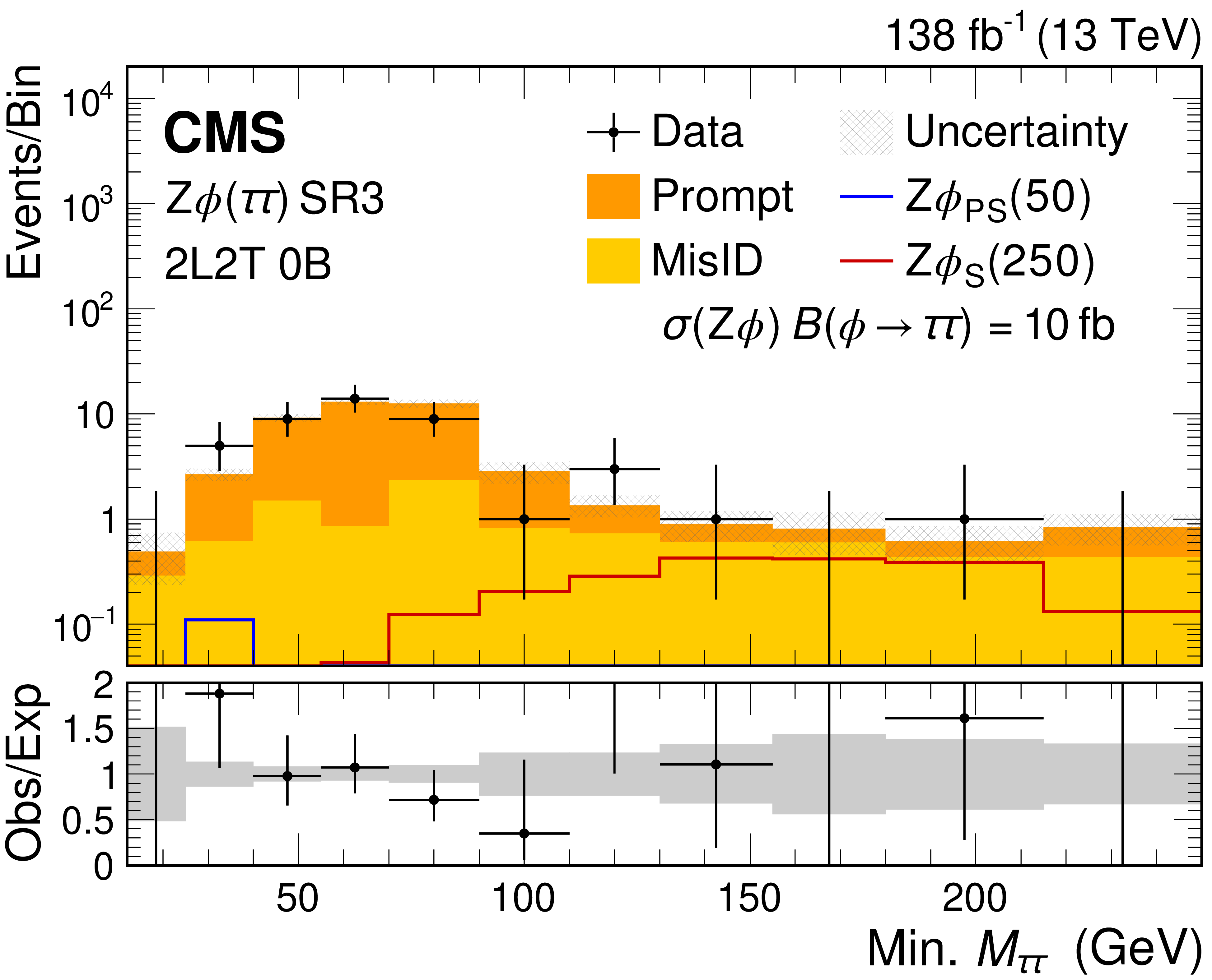
png pdf	Figure 8-f: Dilepton mass spectra for the $ {\mathrm{Z}}{\phi}(\tau\tau) $ SR3 event selection for the combined 2016-2018 data set. The lower panel shows the ratio of observed events to the total expected SM background prediction (Obs/Exp), and the gray band represents the sum of statistical and systematic uncertainties in the background prediction. The rightmost bins contain the overflow events in each distribution. The expected background distributions and the uncertainties are shown after the data is fit under the background-only hypothesis. For illustration, two example signal hypotheses for the production and decay of a scalar and a pseudoscalar $ \phi $ boson are shown, and their masses (in units of GeV) are indicated in the legend. The signals are normalized to the product of the cross section and branching fraction of 10 fb.
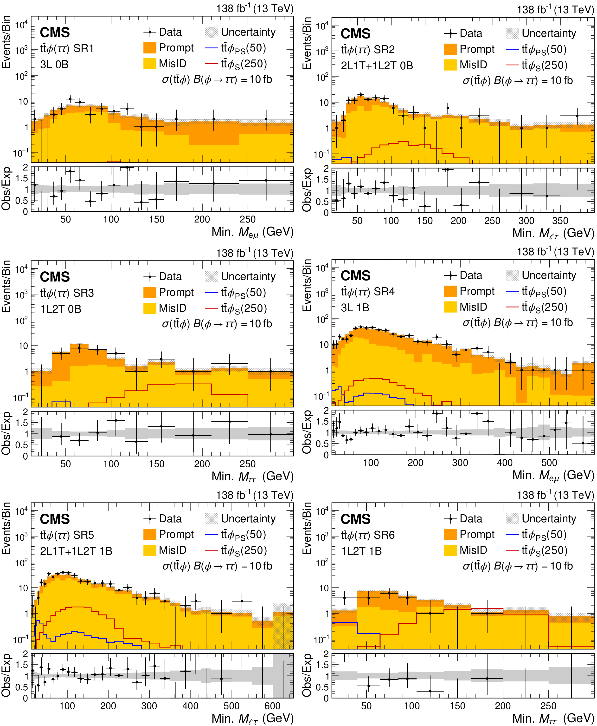
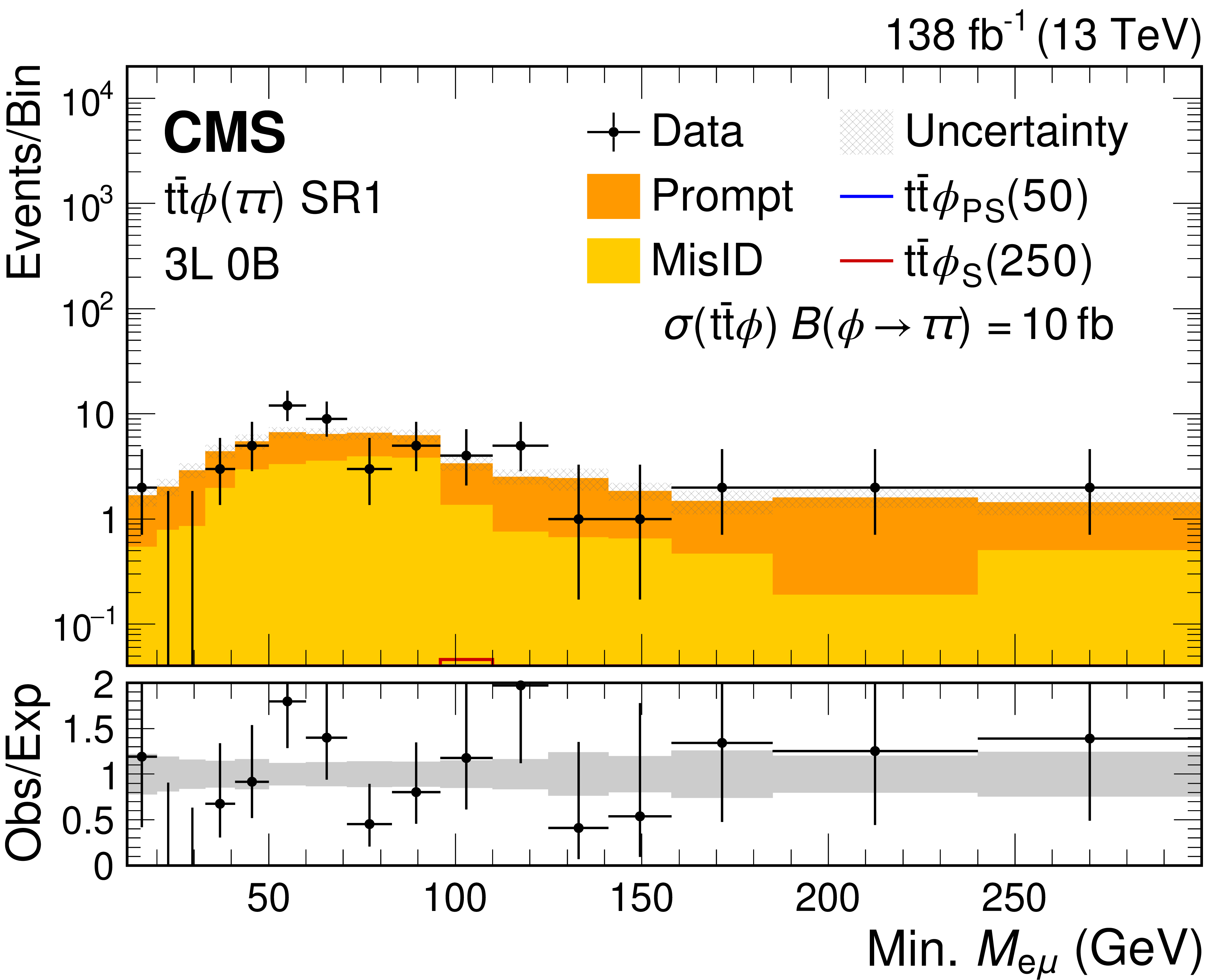
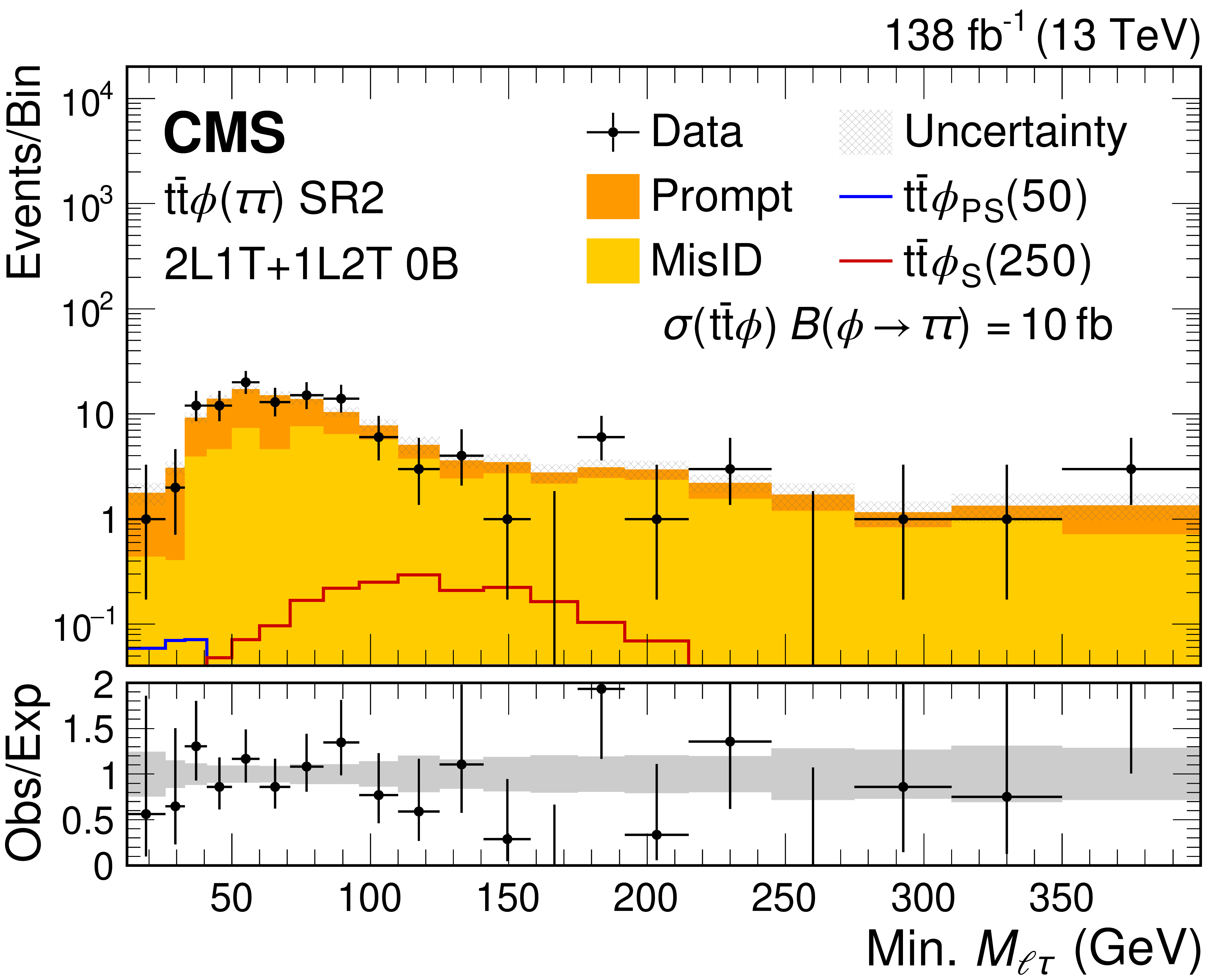
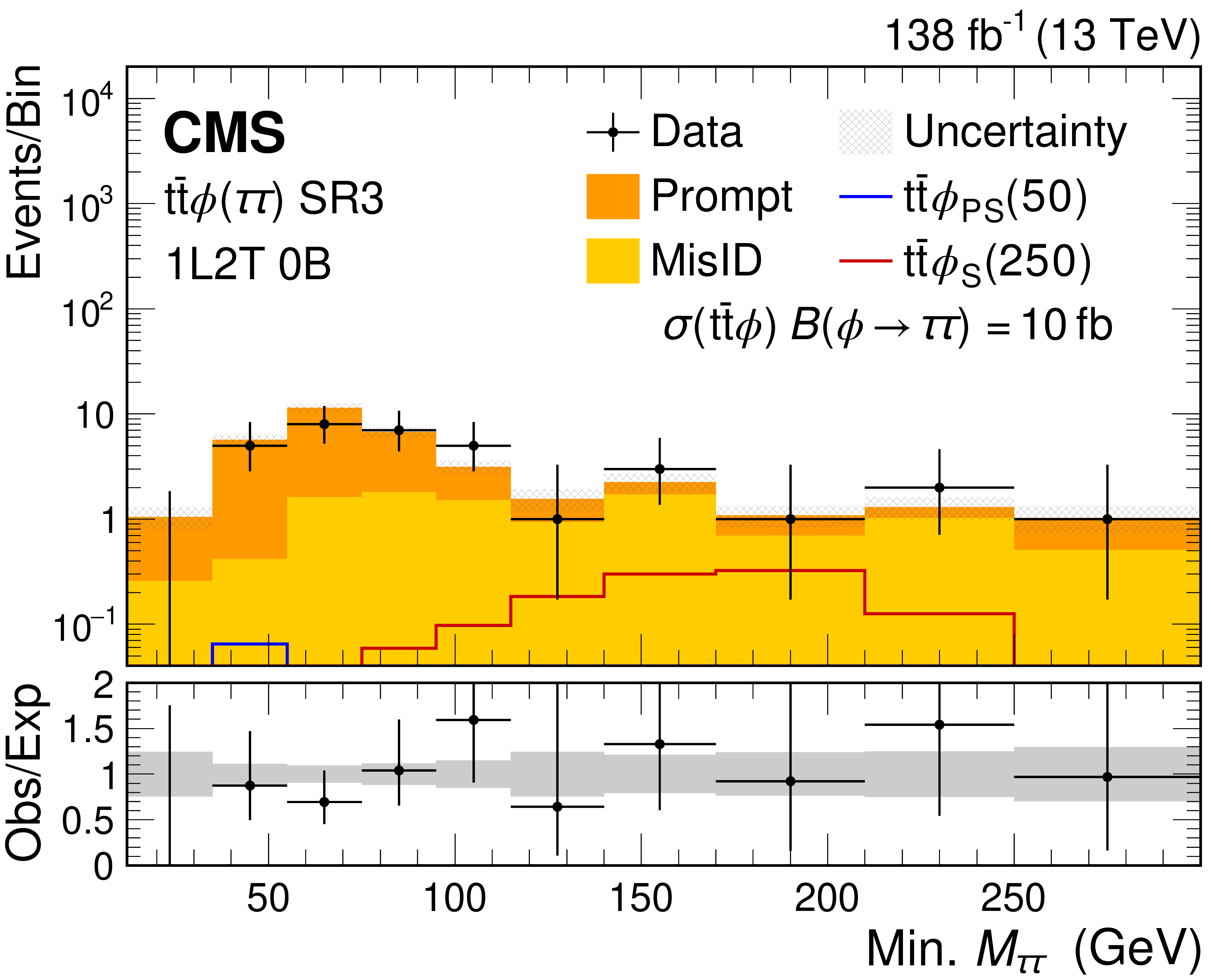
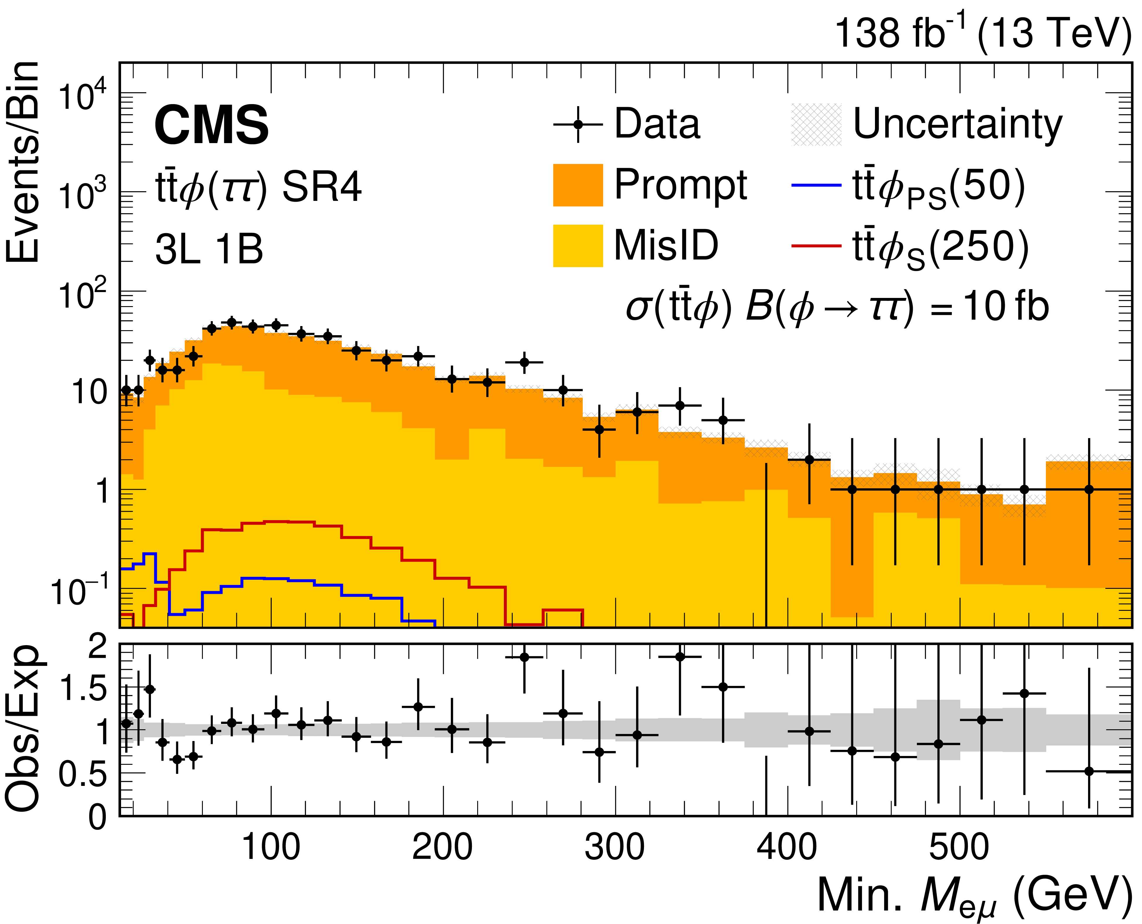
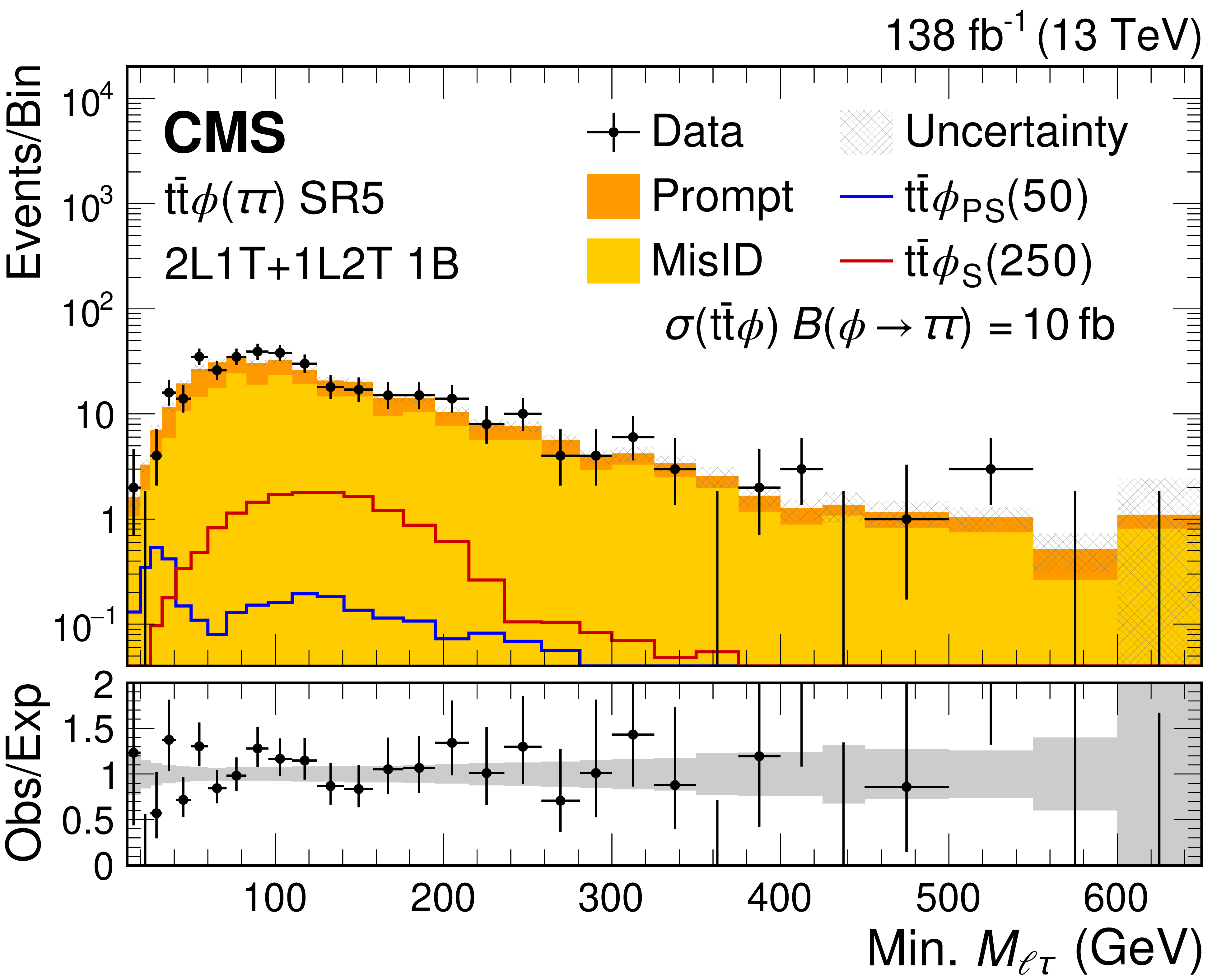
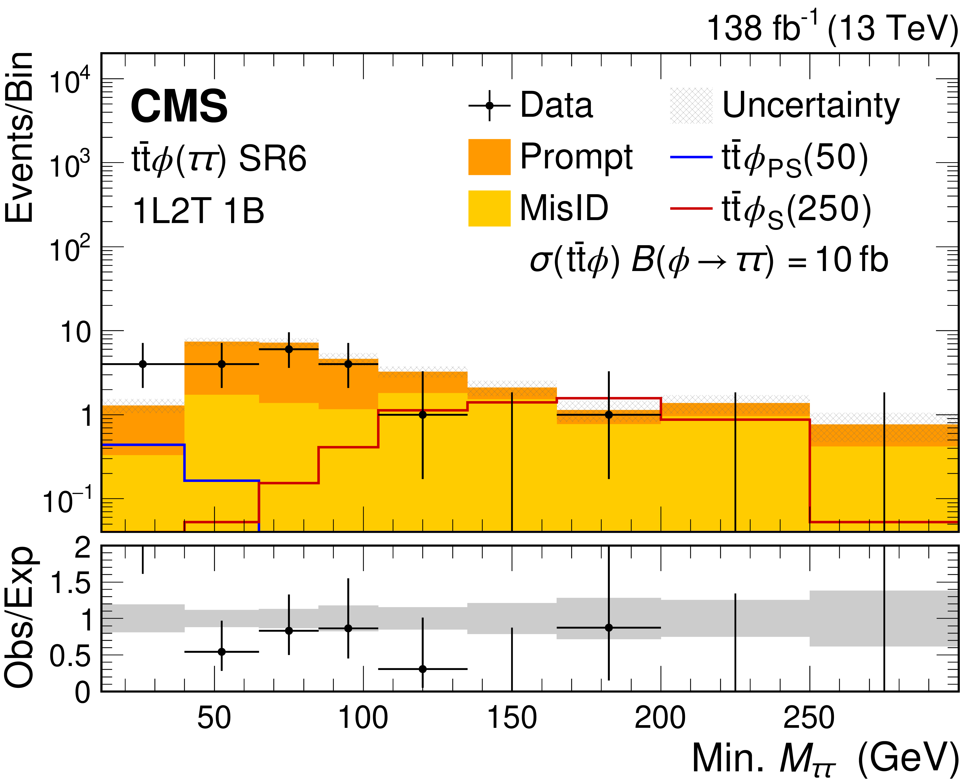
png pdf	Figure 9: Dilepton mass spectra for the $ {{\mathrm{t}\overline{\mathrm{t}}} }{\phi}(\tau\tau) $ SR1-6 event selections for the combined 2016-2018 data set. The lower panel shows the ratio of observed events to the total expected SM background prediction (Obs/Exp), and the gray band represents the sum of statistical and systematic uncertainties in the background prediction. The rightmost bins contain the overflow events in each distribution. The expected background distributions and the uncertainties are shown after the data is fit under the background-only hypothesis. For illustration, two example signal hypotheses for the production and decay of a scalar and a pseudoscalar $ \phi $ boson are shown, and their masses (in units of GeV) are indicated in the legend. The signals are normalized to the product of the cross section and branching fraction of 10 fb.
png pdf	Figure 9-a: Dilepton mass spectrum for the $ {{\mathrm{t}\overline{\mathrm{t}}} }{\phi}(\tau\tau) $ SR1 event selection for the combined 2016-2018 data set. The lower panel shows the ratio of observed events to the total expected SM background prediction (Obs/Exp), and the gray band represents the sum of statistical and systematic uncertainties in the background prediction. The rightmost bins contain the overflow events in each distribution. The expected background distributions and the uncertainties are shown after the data is fit under the background-only hypothesis. For illustration, two example signal hypotheses for the production and decay of a scalar and a pseudoscalar $ \phi $ boson are shown, and their masses (in units of GeV) are indicated in the legend. The signals are normalized to the product of the cross section and branching fraction of 10 fb.
png pdf	Figure 9-b: Dilepton mass spectrum for the $ {{\mathrm{t}\overline{\mathrm{t}}} }{\phi}(\tau\tau) $ SR2 event selection for the combined 2016-2018 data set. The lower panel shows the ratio of observed events to the total expected SM background prediction (Obs/Exp), and the gray band represents the sum of statistical and systematic uncertainties in the background prediction. The rightmost bins contain the overflow events in each distribution. The expected background distributions and the uncertainties are shown after the data is fit under the background-only hypothesis. For illustration, two example signal hypotheses for the production and decay of a scalar and a pseudoscalar $ \phi $ boson are shown, and their masses (in units of GeV) are indicated in the legend. The signals are normalized to the product of the cross section and branching fraction of 10 fb.
png pdf	Figure 9-c: Dilepton mass spectrum for the $ {{\mathrm{t}\overline{\mathrm{t}}} }{\phi}(\tau\tau) $ SR3 event selection for the combined 2016-2018 data set. The lower panel shows the ratio of observed events to the total expected SM background prediction (Obs/Exp), and the gray band represents the sum of statistical and systematic uncertainties in the background prediction. The rightmost bins contain the overflow events in each distribution. The expected background distributions and the uncertainties are shown after the data is fit under the background-only hypothesis. For illustration, two example signal hypotheses for the production and decay of a scalar and a pseudoscalar $ \phi $ boson are shown, and their masses (in units of GeV) are indicated in the legend. The signals are normalized to the product of the cross section and branching fraction of 10 fb.
png pdf	Figure 9-d: Dilepton mass spectrum for the $ {{\mathrm{t}\overline{\mathrm{t}}} }{\phi}(\tau\tau) $ SR4 event selection for the combined 2016-2018 data set. The lower panel shows the ratio of observed events to the total expected SM background prediction (Obs/Exp), and the gray band represents the sum of statistical and systematic uncertainties in the background prediction. The rightmost bins contain the overflow events in each distribution. The expected background distributions and the uncertainties are shown after the data is fit under the background-only hypothesis. For illustration, two example signal hypotheses for the production and decay of a scalar and a pseudoscalar $ \phi $ boson are shown, and their masses (in units of GeV) are indicated in the legend. The signals are normalized to the product of the cross section and branching fraction of 10 fb.
png pdf	Figure 9-e: Dilepton mass spectrum for the $ {{\mathrm{t}\overline{\mathrm{t}}} }{\phi}(\tau\tau) $ SR5 event selection for the combined 2016-2018 data set. The lower panel shows the ratio of observed events to the total expected SM background prediction (Obs/Exp), and the gray band represents the sum of statistical and systematic uncertainties in the background prediction. The rightmost bins contain the overflow events in each distribution. The expected background distributions and the uncertainties are shown after the data is fit under the background-only hypothesis. For illustration, two example signal hypotheses for the production and decay of a scalar and a pseudoscalar $ \phi $ boson are shown, and their masses (in units of GeV) are indicated in the legend. The signals are normalized to the product of the cross section and branching fraction of 10 fb.
png pdf	Figure 9-f: Dilepton mass spectrum for the $ {{\mathrm{t}\overline{\mathrm{t}}} }{\phi}(\tau\tau) $ SR6 event selection for the combined 2016-2018 data set. The lower panel shows the ratio of observed events to the total expected SM background prediction (Obs/Exp), and the gray band represents the sum of statistical and systematic uncertainties in the background prediction. The rightmost bins contain the overflow events in each distribution. The expected background distributions and the uncertainties are shown after the data is fit under the background-only hypothesis. For illustration, two example signal hypotheses for the production and decay of a scalar and a pseudoscalar $ \phi $ boson are shown, and their masses (in units of GeV) are indicated in the legend. The signals are normalized to the product of the cross section and branching fraction of 10 fb.
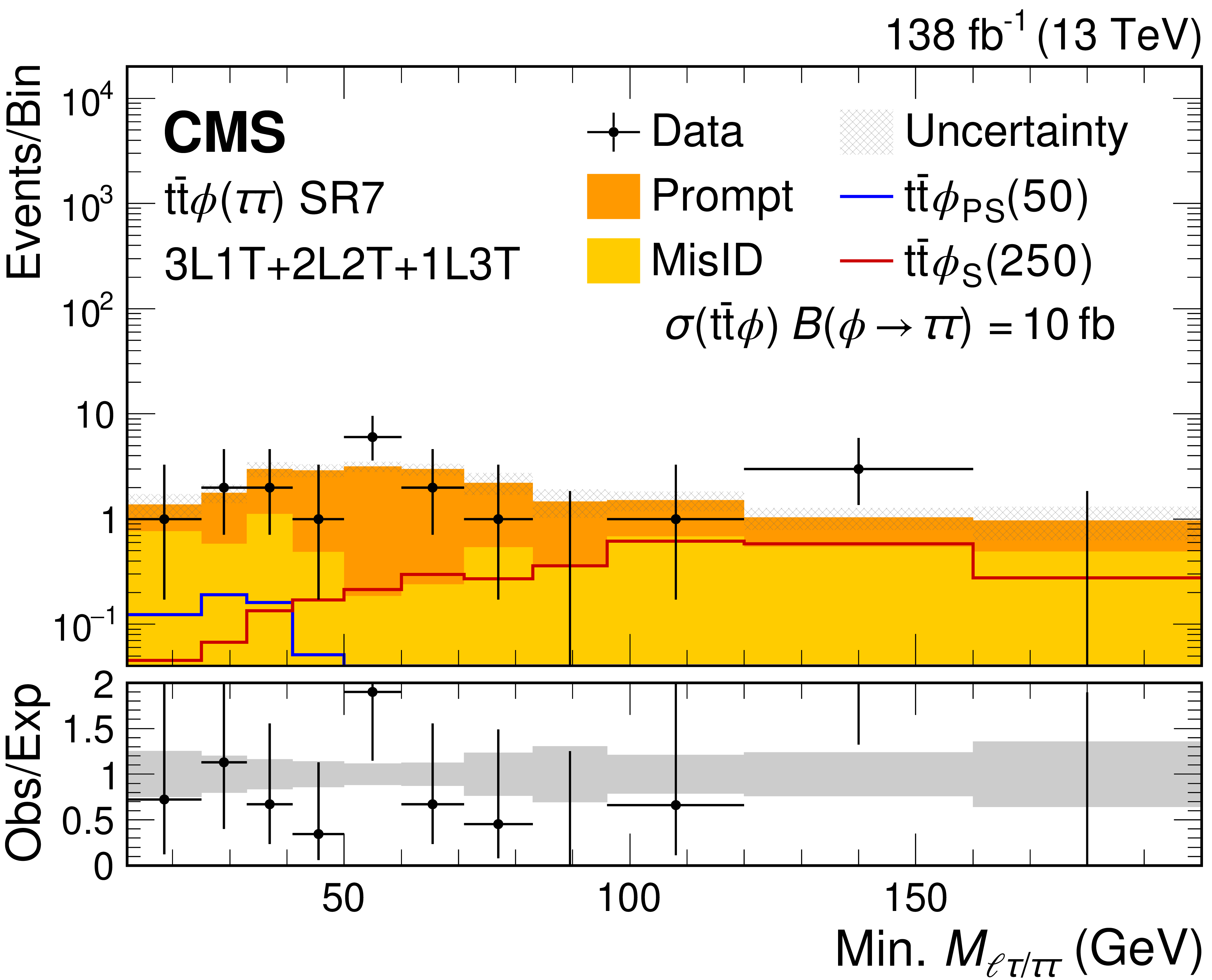
png pdf	Figure 10: Dilepton mass spectra for the $ {{\mathrm{t}\overline{\mathrm{t}}} }{\phi}(\tau\tau) $ SR7 event selection for the combined 2016-2018 data set. The lower panel shows the ratio of observed events to the total expected SM background prediction (Obs/Exp), and the gray band represents the sum of statistical and systematic uncertainties in the background prediction. The rightmost bins contain the overflow events in each distribution. The expected background distributions and the uncertainties are shown after the data is fit under the background-only hypothesis. For illustration, two example signal hypotheses for the production and decay of a scalar and a pseudoscalar $ \phi $ boson are shown, and their masses (in units of GeV) are indicated in the legend. The signals are normalized to the product of the cross section and branching fraction of 10 fb.
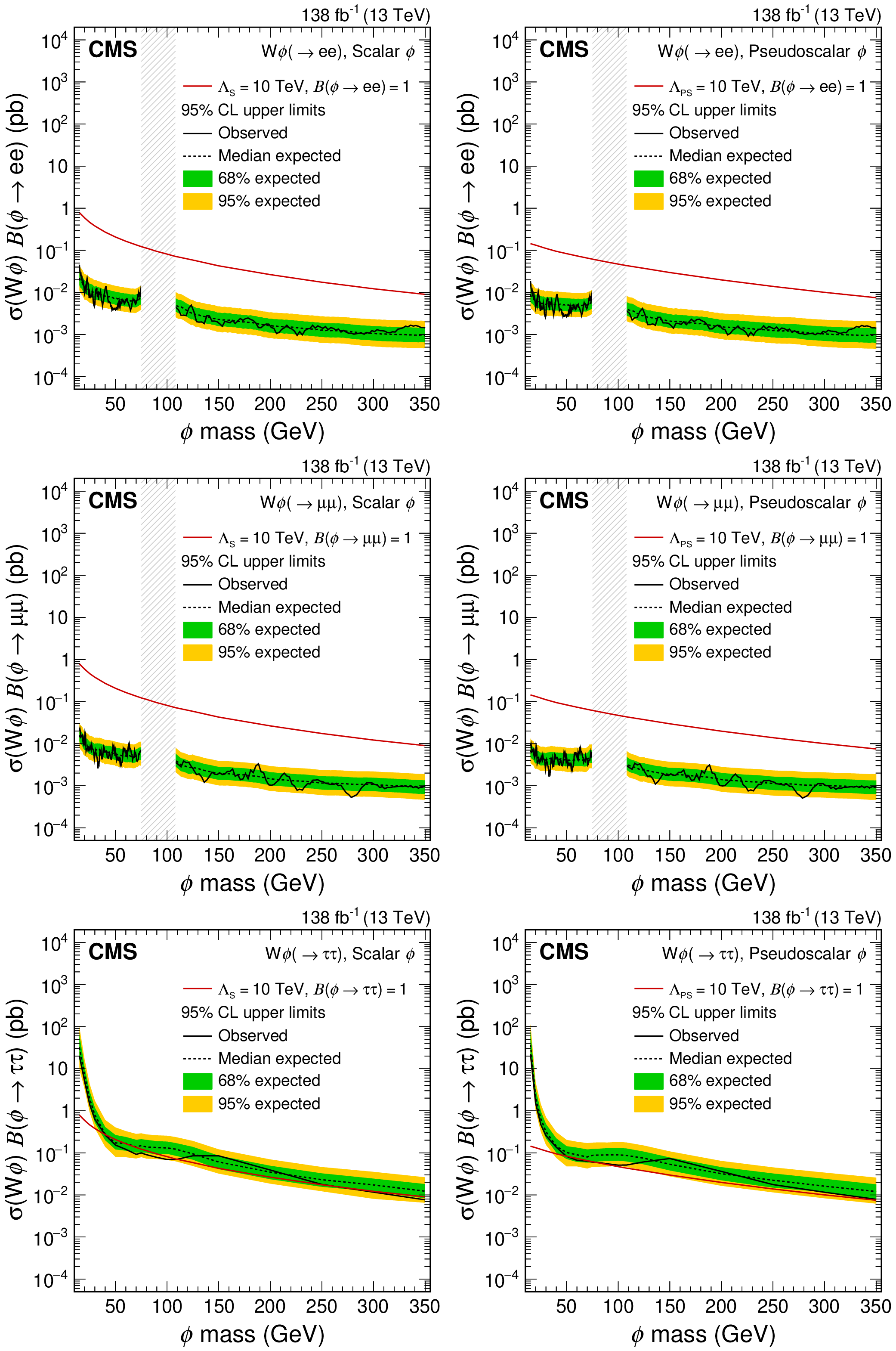
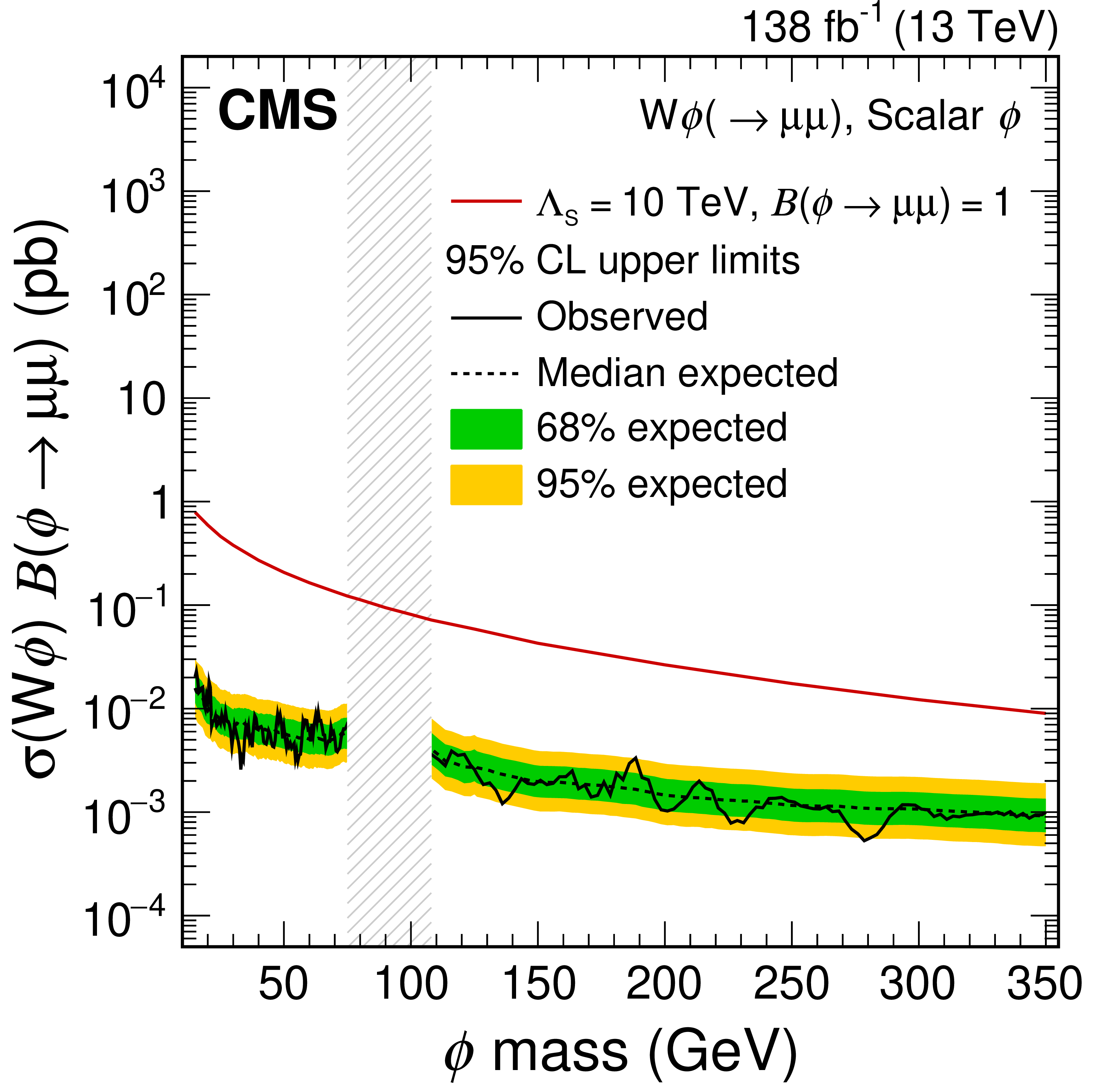
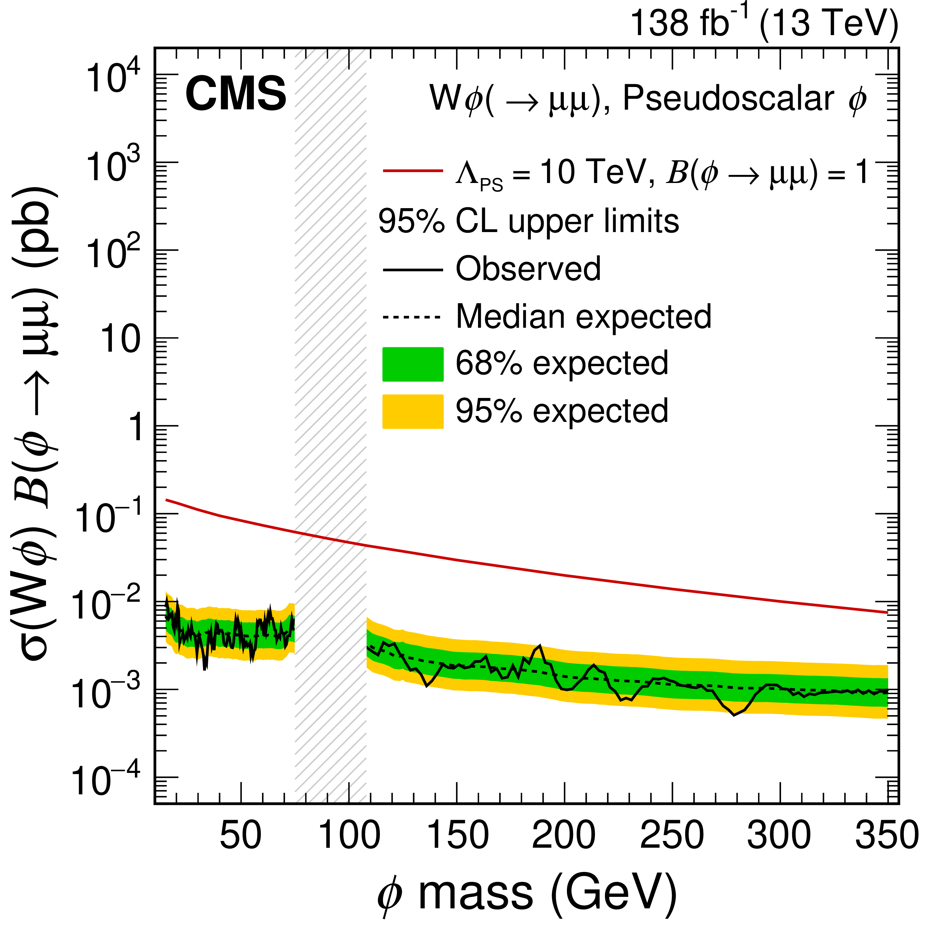
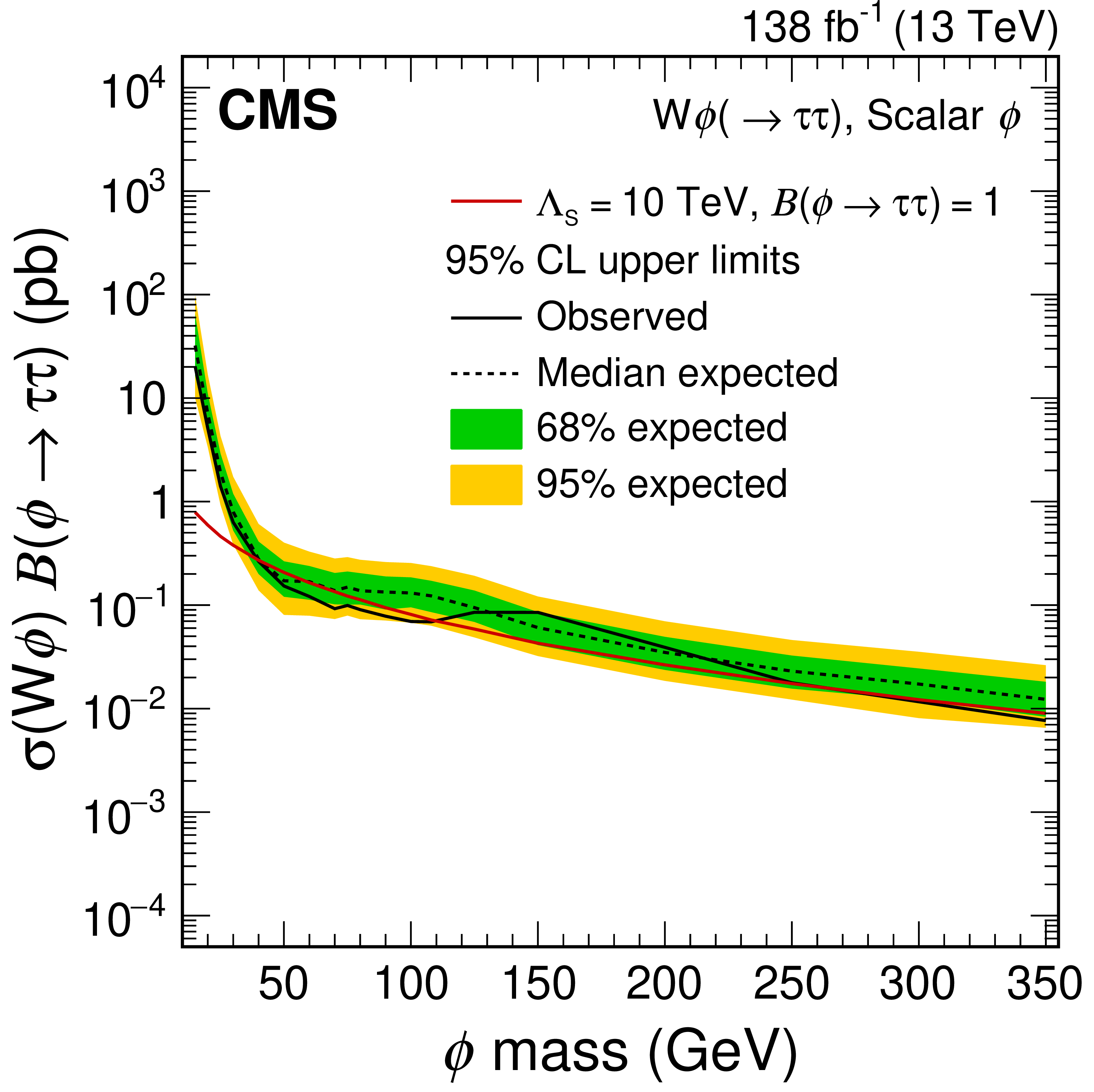
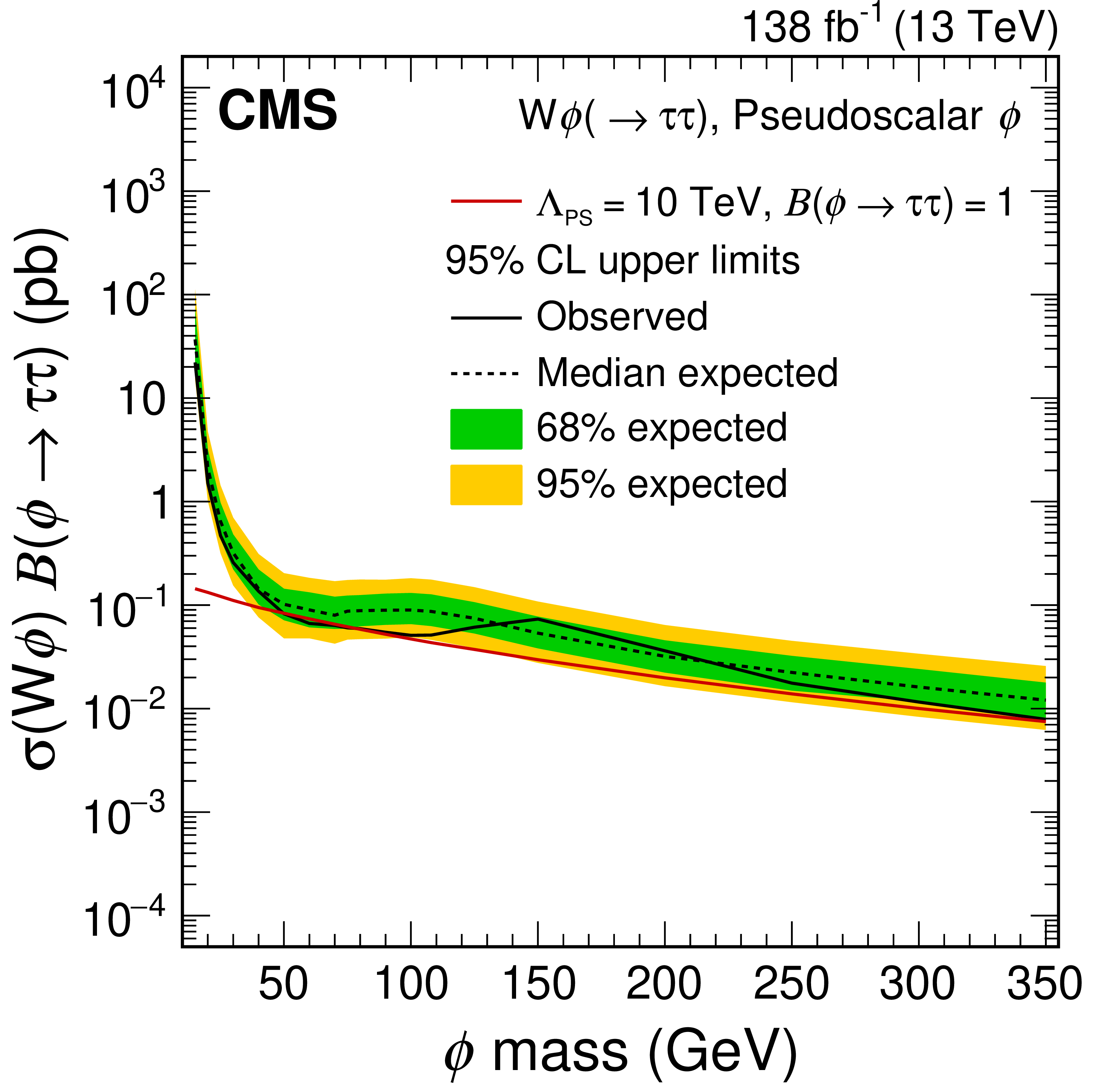
png pdf	Figure 11: The 95% confidence level upper limits on the product of the production cross section and branching fraction of the $ {\mathrm{W}}{\phi} $ signal in the $ \mathrm{e}\mathrm{e} $ (upper), $ \mu\mu $ (middle), and $ \tau\tau $ (lower) decay scenarios. The results for the scalar coupling are shown on the left and pseudoscalar on the right. The vertical gray band indicates the mass region not considered in the analysis. The red line is the theoretical prediction for the product of the production cross section and branching fraction of the $ {\mathrm{W}}{\phi} $ signal.
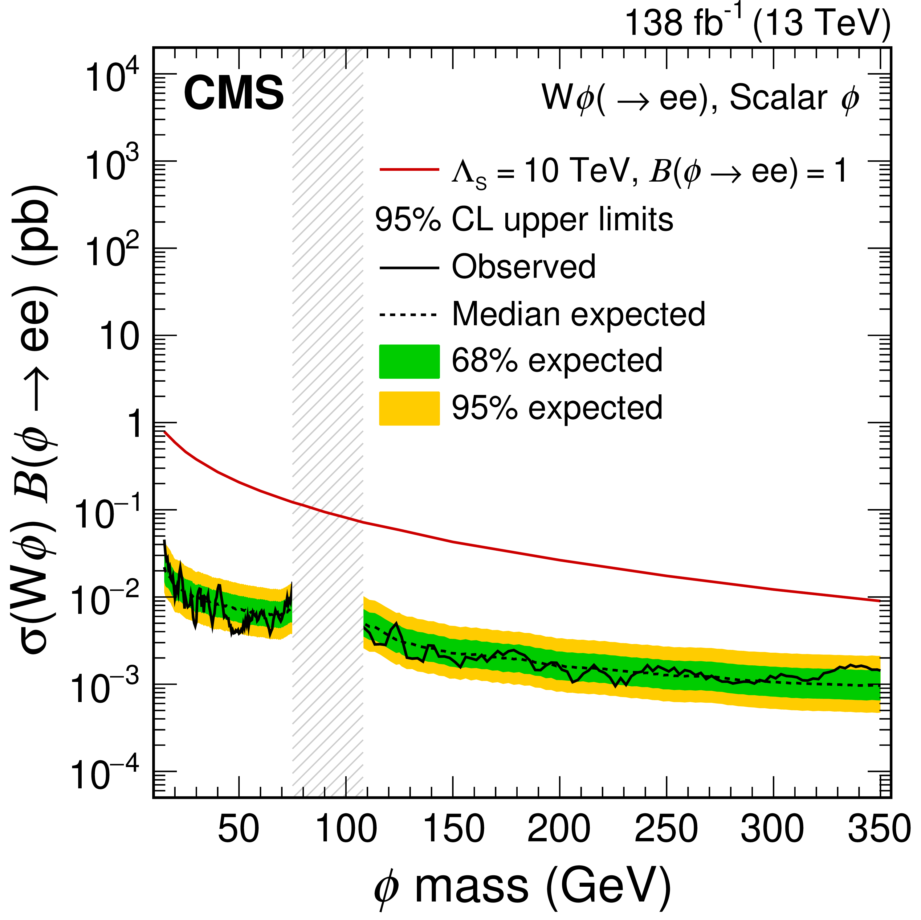
png pdf	Figure 11-a: The 95% confidence level upper limits on the product of the production cross section and branching fraction of the $ {\mathrm{W}}{\phi} $ signal in the $ \mathrm{e}\mathrm{e} $ decay scenario, for the scalar coupling. The vertical gray band indicates the mass region not considered in the analysis. The red line is the theoretical prediction for the product of the production cross section and branching fraction of the $ {\mathrm{W}}{\phi} $ signal.
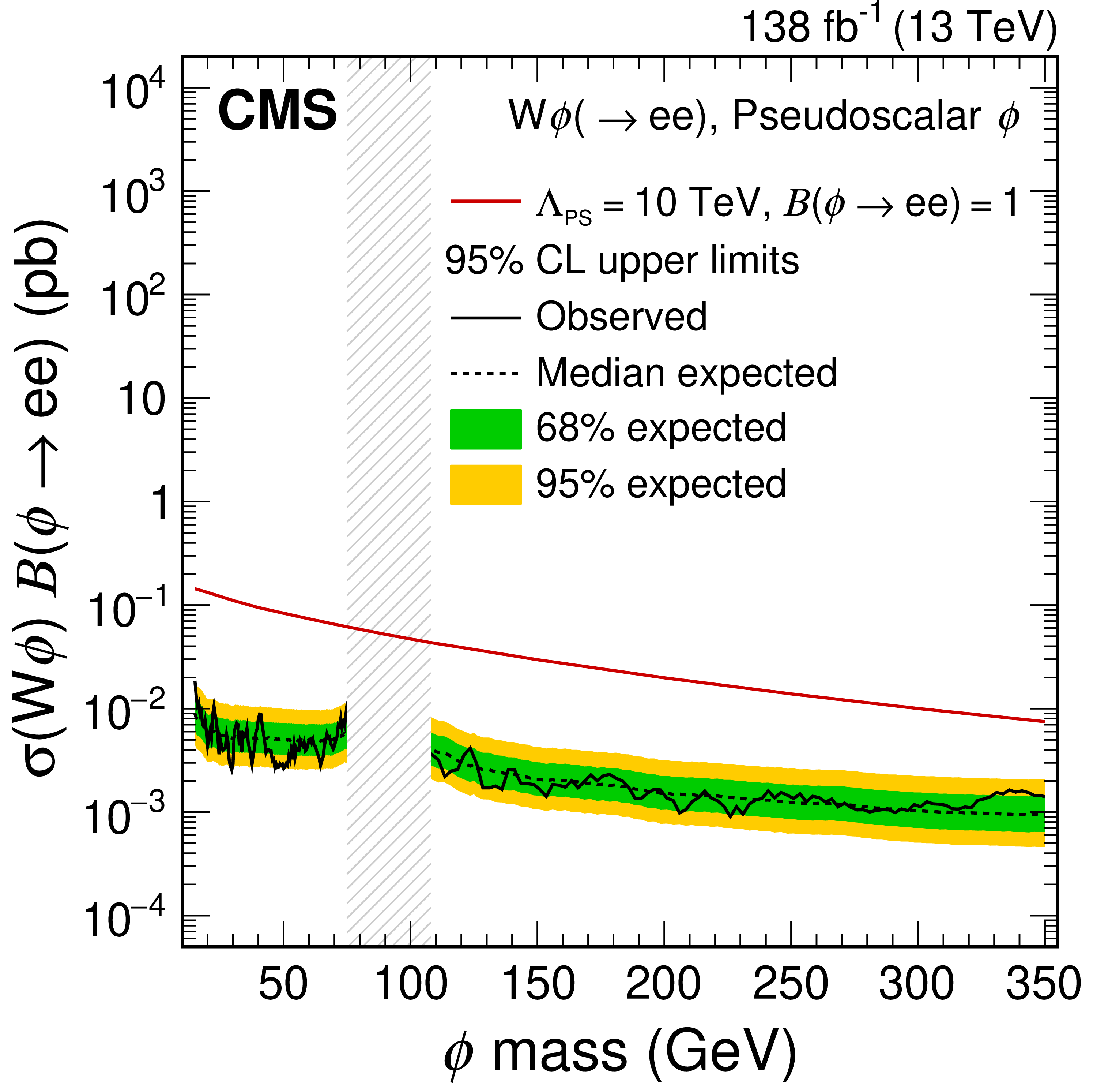
png pdf	Figure 11-b: The 95% confidence level upper limits on the product of the production cross section and branching fraction of the $ {\mathrm{W}}{\phi} $ signal in the $ \mathrm{e}\mathrm{e} $ decay scenario, for the pseudoscalar coupling. The vertical gray band indicates the mass region not considered in the analysis. The red line is the theoretical prediction for the product of the production cross section and branching fraction of the $ {\mathrm{W}}{\phi} $ signal.
png pdf	Figure 11-c: The 95% confidence level upper limits on the product of the production cross section and branching fraction of the $ {\mathrm{W}}{\phi} $ signal in the $ \mu\mu $ decay scenario, for the scalar coupling. The vertical gray band indicates the mass region not considered in the analysis. The red line is the theoretical prediction for the product of the production cross section and branching fraction of the $ {\mathrm{W}}{\phi} $ signal.
png pdf	Figure 11-d: The 95% confidence level upper limits on the product of the production cross section and branching fraction of the $ {\mathrm{W}}{\phi} $ signal in the $ \mu\mu $ decay scenario, for the pseudoscalar coupling. The vertical gray band indicates the mass region not considered in the analysis. The red line is the theoretical prediction for the product of the production cross section and branching fraction of the $ {\mathrm{W}}{\phi} $ signal.
png pdf	Figure 11-e: The 95% confidence level upper limits on the product of the production cross section and branching fraction of the $ {\mathrm{W}}{\phi} $ signal in the $ \tau\tau $ decay scenario, for the scalar coupling. The vertical gray band indicates the mass region not considered in the analysis. The red line is the theoretical prediction for the product of the production cross section and branching fraction of the $ {\mathrm{W}}{\phi} $ signal.
png pdf	Figure 11-f: The 95% confidence level upper limits on the product of the production cross section and branching fraction of the $ {\mathrm{W}}{\phi} $ signal in the $ \tau\tau $ decay scenario, for the pseudoscalar coupling. The vertical gray band indicates the mass region not considered in the analysis. The red line is the theoretical prediction for the product of the production cross section and branching fraction of the $ {\mathrm{W}}{\phi} $ signal.
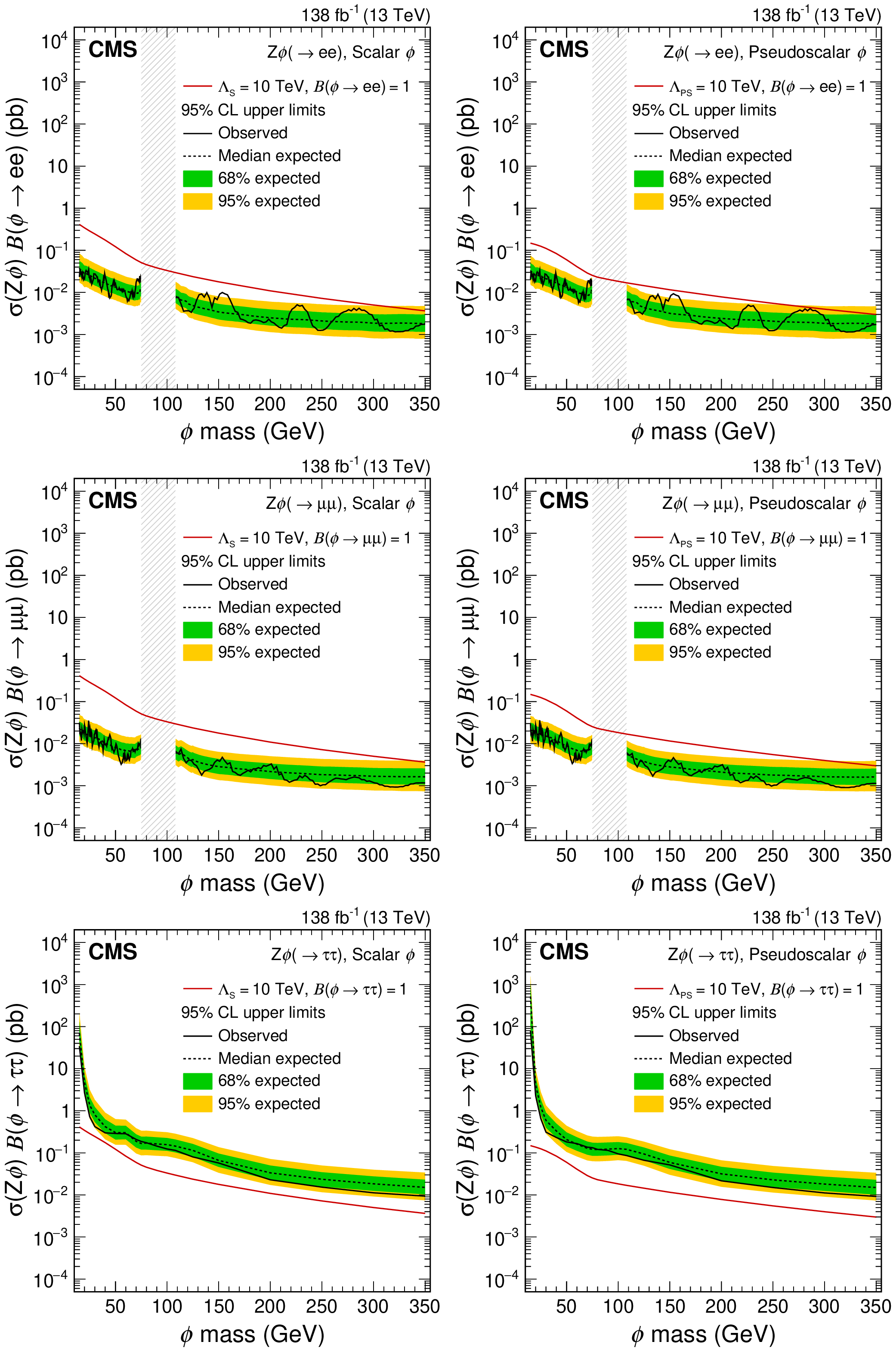
png pdf	Figure 12: The 95% confidence level upper limits on the product of the production cross section and branching fraction of the $ {\mathrm{Z}}{\phi} $ signal in the $ \mathrm{e}\mathrm{e} $ (upper), $ \mu\mu $ (middle) and $ \tau\tau $ (lower) decay scenarios. The results for the scalar coupling are shown on the left and pseudoscalar on the right. The vertical gray band indicates the mass region not considered in the analysis. The red line is the theoretical prediction for the product of the production cross section and branching fraction of the $ {\mathrm{Z}}{\phi} $ signal.
png pdf	Figure 12-a: The 95% confidence level upper limits on the product of the production cross section and branching fraction of the $ {\mathrm{Z}}{\phi} $ signal in the $ \mathrm{e}\mathrm{e} $ decay scenario, for the scalar coupling. The vertical gray band indicates the mass region not considered in the analysis. The red line is the theoretical prediction for the product of the production cross section and branching fraction of the $ {\mathrm{Z}}{\phi} $ signal.
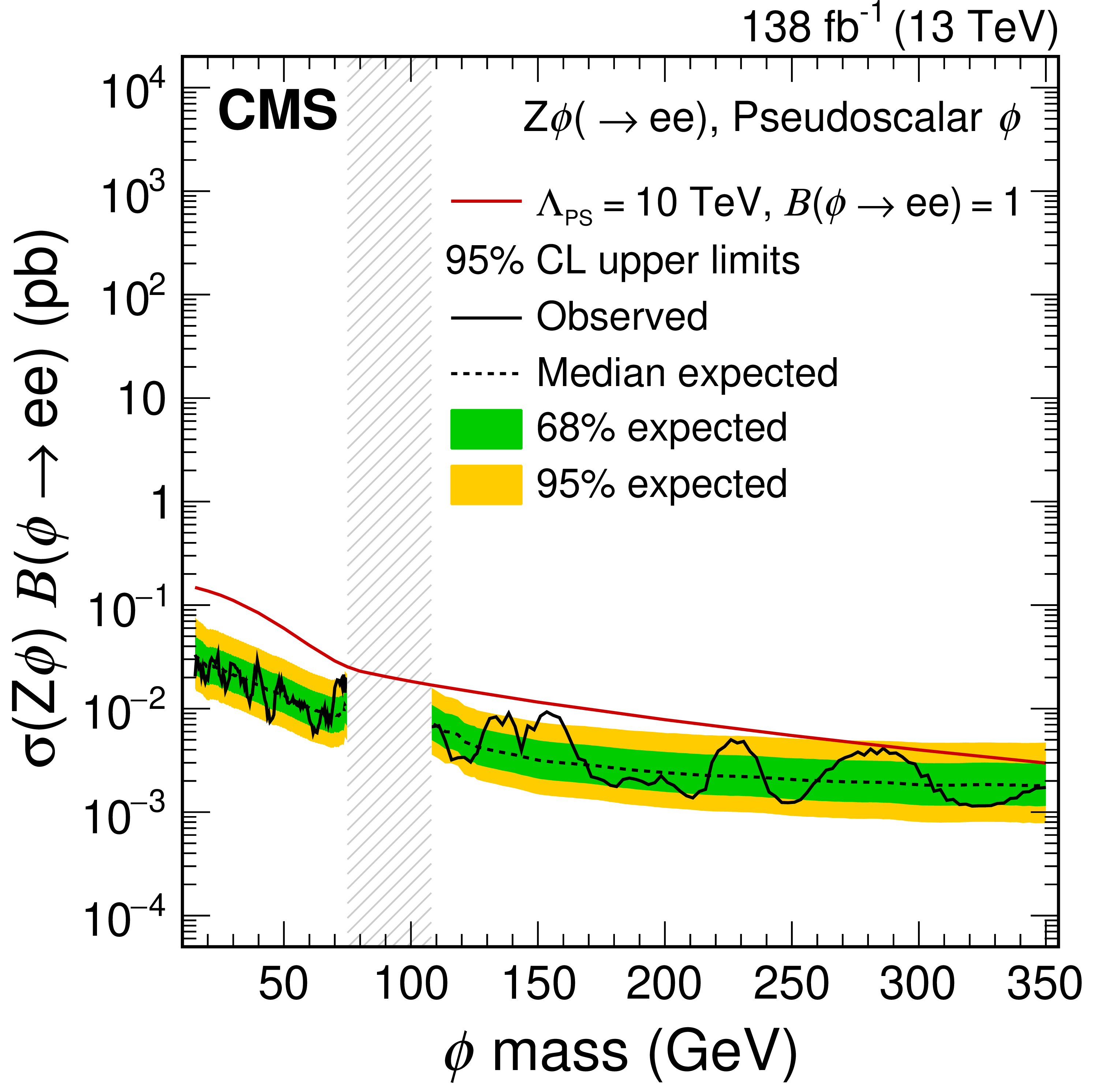
png pdf	Figure 12-b: The 95% confidence level upper limits on the product of the production cross section and branching fraction of the $ {\mathrm{Z}}{\phi} $ signal in the $ \mathrm{e}\mathrm{e} $ decay scenario, for the pseudoscalar coupling. The vertical gray band indicates the mass region not considered in the analysis. The red line is the theoretical prediction for the product of the production cross section and branching fraction of the $ {\mathrm{Z}}{\phi} $ signal.
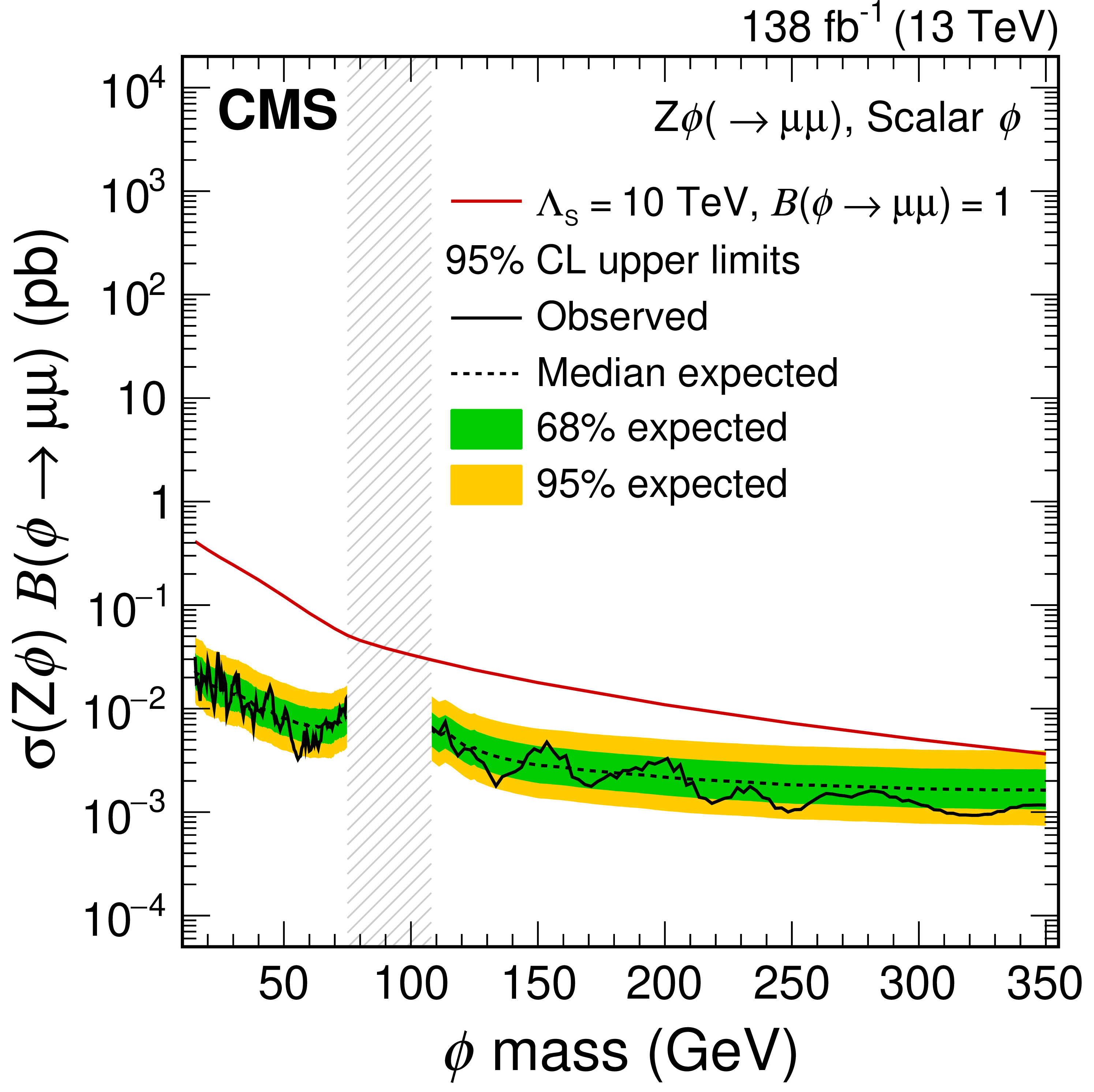
png pdf	Figure 12-c: The 95% confidence level upper limits on the product of the production cross section and branching fraction of the $ {\mathrm{Z}}{\phi} $ signal in the $ \mu\mu $ decay scenario, for the scalar coupling. The vertical gray band indicates the mass region not considered in the analysis. The red line is the theoretical prediction for the product of the production cross section and branching fraction of the $ {\mathrm{Z}}{\phi} $ signal.
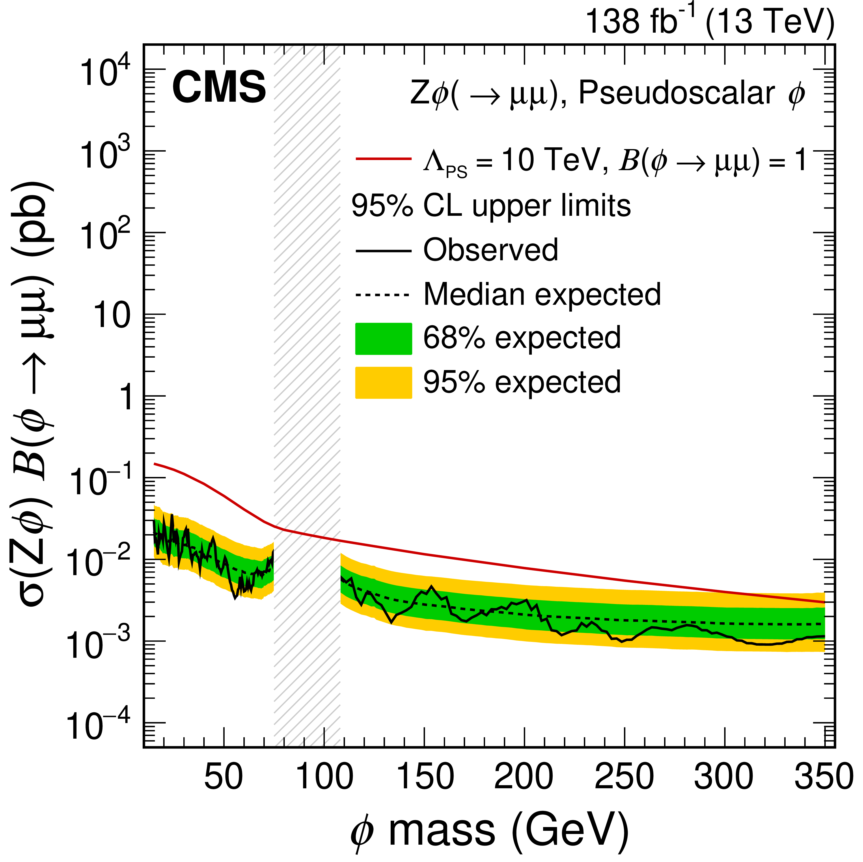
png pdf	Figure 12-d: The 95% confidence level upper limits on the product of the production cross section and branching fraction of the $ {\mathrm{Z}}{\phi} $ signal in the $ \mu\mu $ decay scenario, for the pseudoscalar coupling. The vertical gray band indicates the mass region not considered in the analysis. The red line is the theoretical prediction for the product of the production cross section and branching fraction of the $ {\mathrm{Z}}{\phi} $ signal.
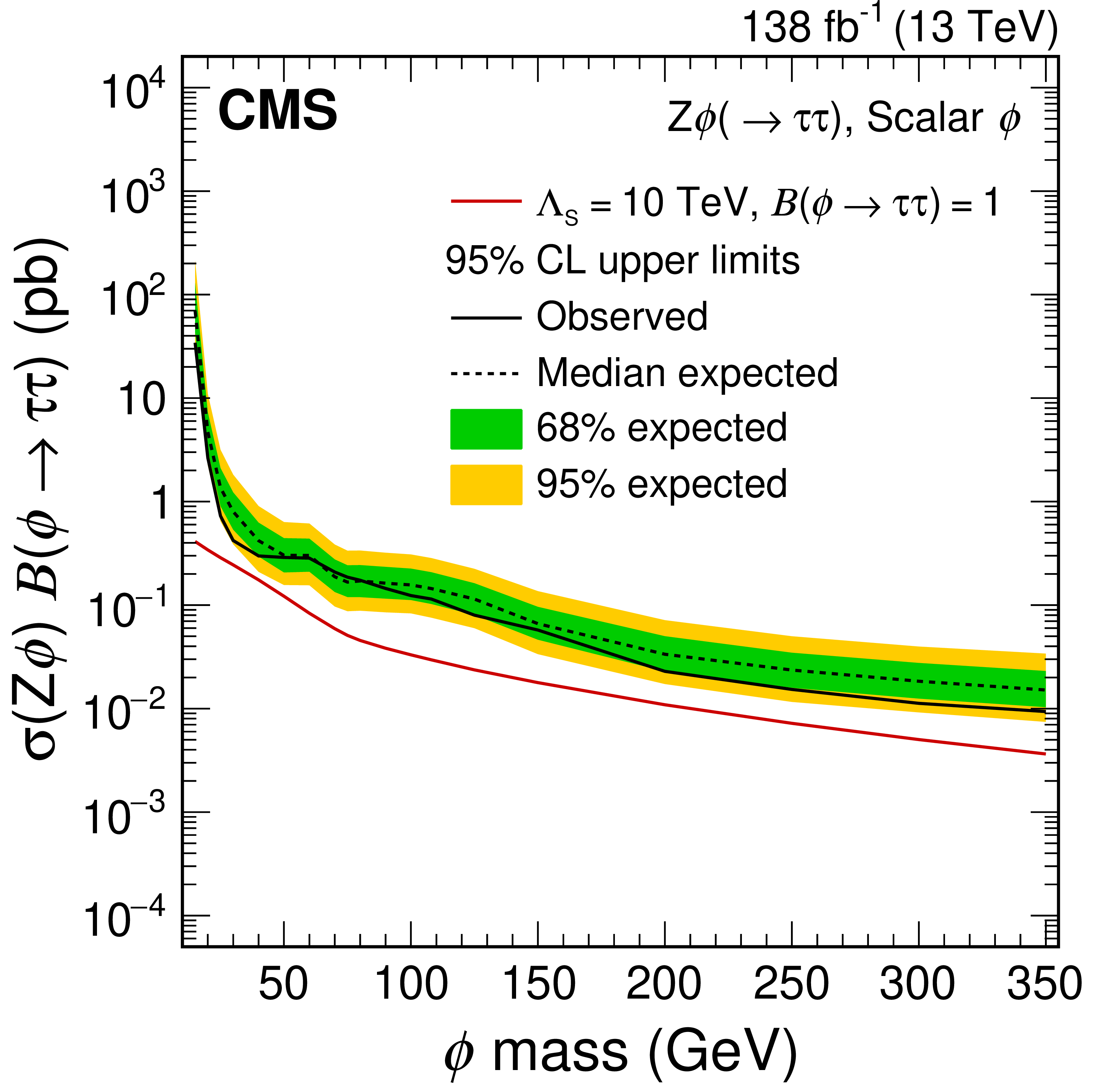
png pdf	Figure 12-e: The 95% confidence level upper limits on the product of the production cross section and branching fraction of the $ {\mathrm{Z}}{\phi} $ signal in the $ \tau\tau $ decay scenario, for the scalar coupling. The vertical gray band indicates the mass region not considered in the analysis. The red line is the theoretical prediction for the product of the production cross section and branching fraction of the $ {\mathrm{Z}}{\phi} $ signal.
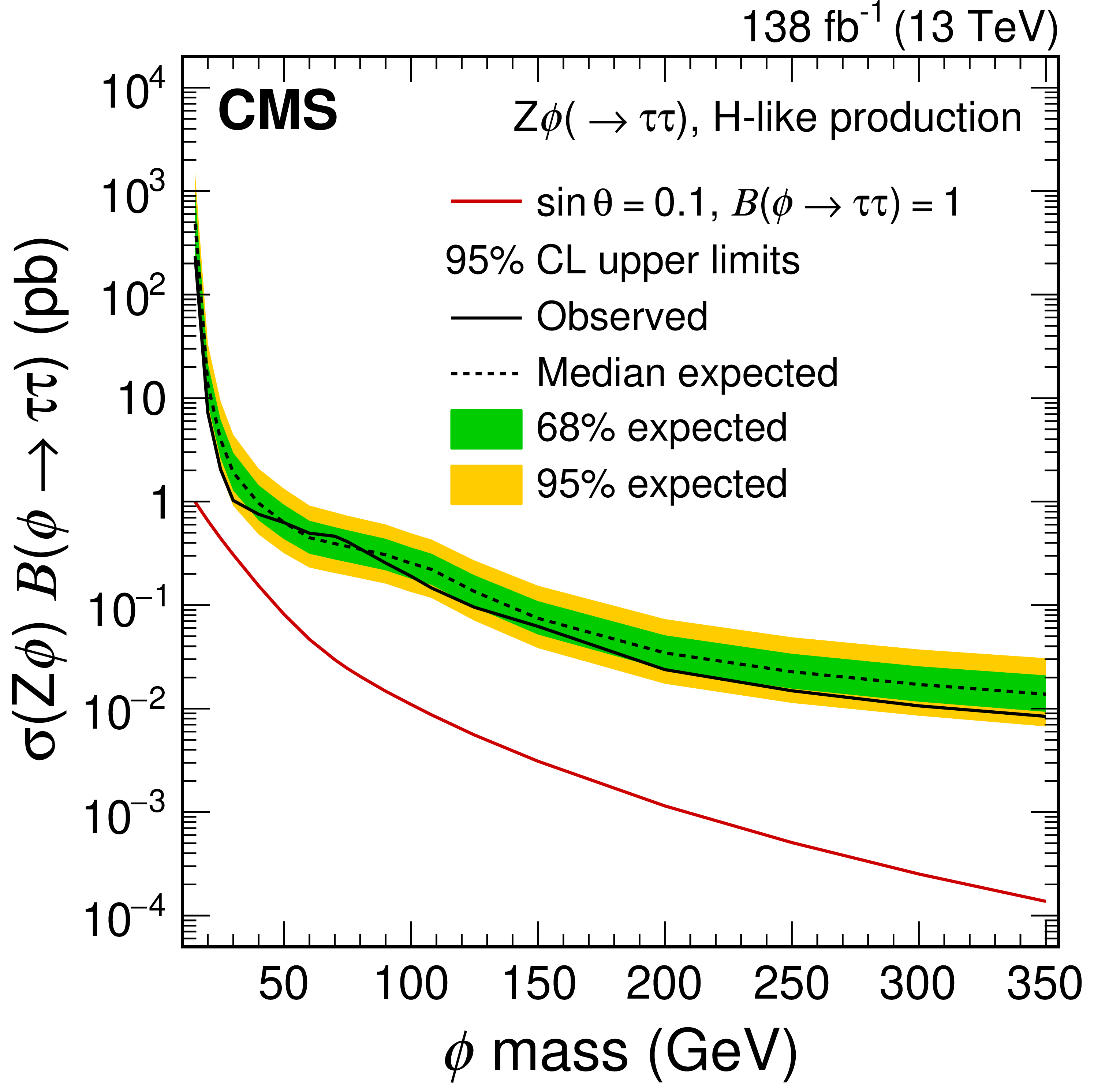
png pdf	Figure 12-f: The 95% confidence level upper limits on the product of the production cross section and branching fraction of the $ {\mathrm{Z}}{\phi} $ signal in the $ \tau\tau $ decay scenario, for the pseudoscalar coupling. The vertical gray band indicates the mass region not considered in the analysis. The red line is the theoretical prediction for the product of the production cross section and branching fraction of the $ {\mathrm{Z}}{\phi} $ signal.
png pdf	Figure 13: The 95% confidence level upper limits on the product of the production cross section and branching fraction of the $ {\mathrm{W}}{\phi} $ signal on the left and the $ {\mathrm{Z}}{\phi} $ signal on the right with H-like couplings in the $ \mathrm{e}\mathrm{e} $ (upper), $ \mu\mu $ (middle) and $ \tau\tau $ (lower) decay scenarios. The vertical gray band indicates the mass region not considered in the analysis. The red line is the theoretical prediction for the product of the production cross section and branching fraction of the $ {\mathrm{W}}{\phi} $ and $ {\mathrm{Z}}{\phi} $ signals.
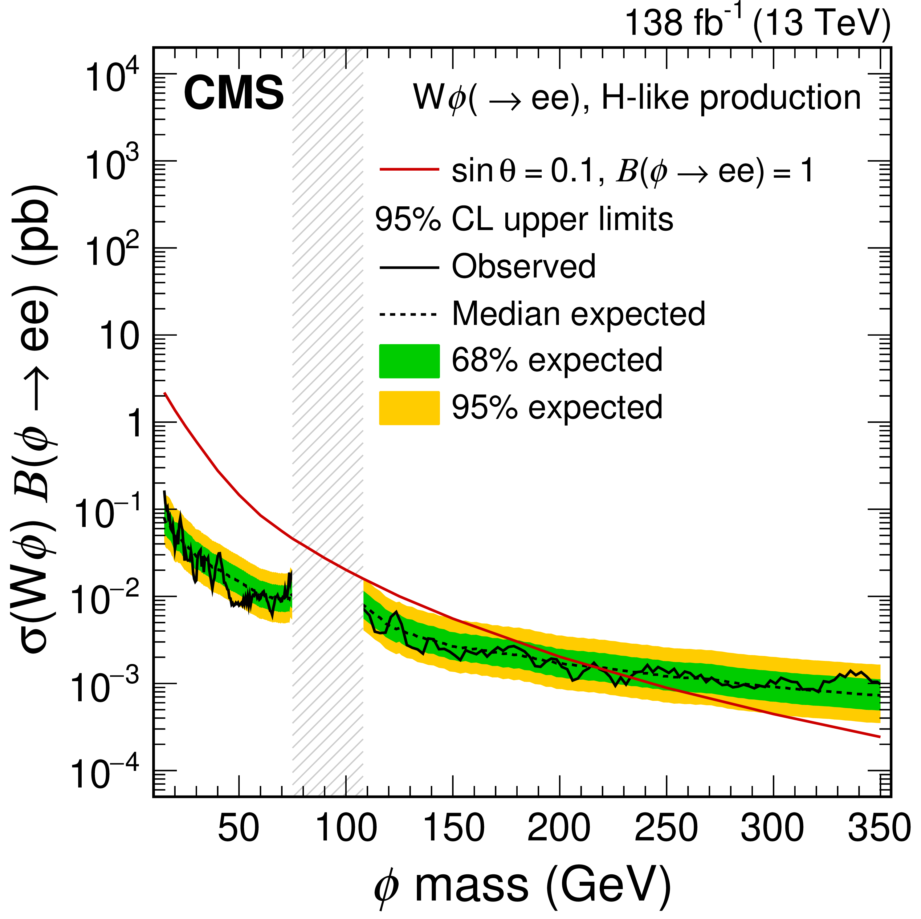
png pdf	Figure 13-a: The 95% confidence level upper limits on the product of the production cross section and branching fraction of the $ {\mathrm{W}}{\phi} $ signal with H-like couplings in the $ \mathrm{e}\mathrm{e} $ decay scenario. The vertical gray band indicates the mass region not considered in the analysis. The red line is the theoretical prediction for the product of the production cross section and branching fraction of the $ {\mathrm{W}}{\phi} $ signal.
png pdf	Figure 13-b: The 95% confidence level upper limits on the product of the production cross section and branching fraction of the $ {\mathrm{Z}}{\phi} $ signal with H-like couplings in the $ \mathrm{e}\mathrm{e} $ decay scenario. The vertical gray band indicates the mass region not considered in the analysis. The red line is the theoretical prediction for the product of the production cross section and branching fraction of the $ {\mathrm{Z}}{\phi} $ signal.
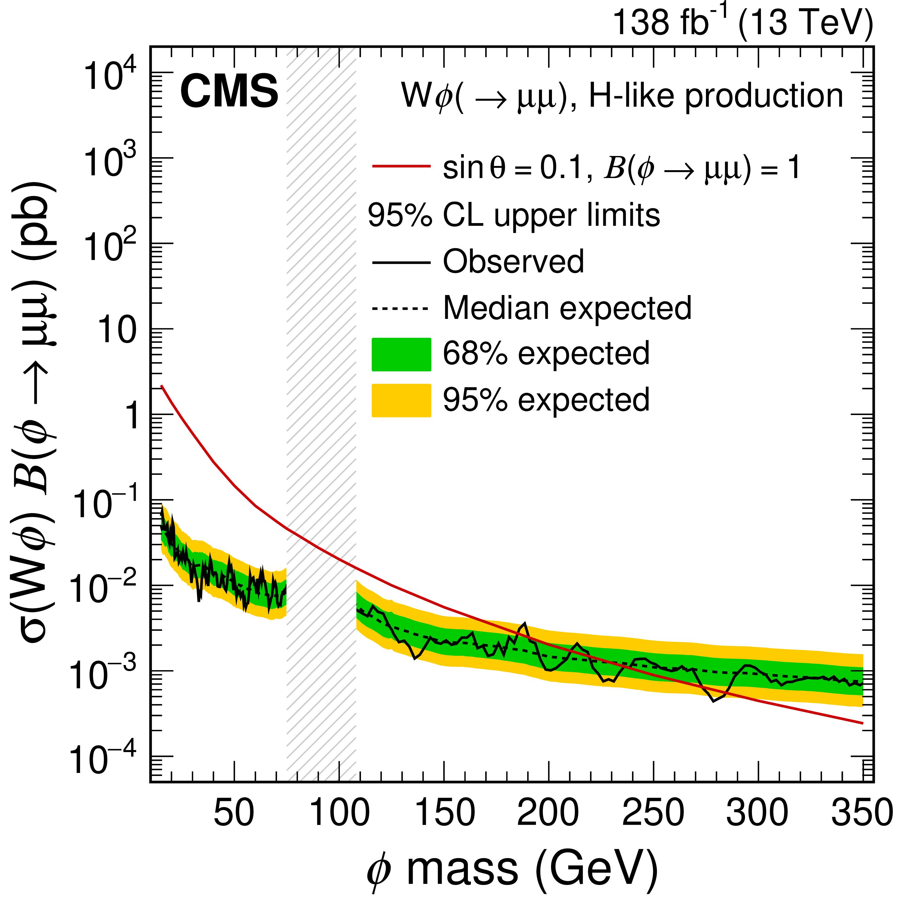
png pdf	Figure 13-c: The 95% confidence level upper limits on the product of the production cross section and branching fraction of the $ {\mathrm{W}}{\phi} $ signal with H-like couplings in the $ \mu\mu $ decay scenario. The vertical gray band indicates the mass region not considered in the analysis. The red line is the theoretical prediction for the product of the production cross section and branching fraction of the $ {\mathrm{W}}{\phi} $ signal.
png pdf	Figure 13-d: The 95% confidence level upper limits on the product of the production cross section and branching fraction of the $ {\mathrm{Z}}{\phi} $ signal with H-like couplings in the $ \mu\mu $ decay scenario. The vertical gray band indicates the mass region not considered in the analysis. The red line is the theoretical prediction for the product of the production cross section and branching fraction of the $ {\mathrm{Z}}{\phi} $ signal.
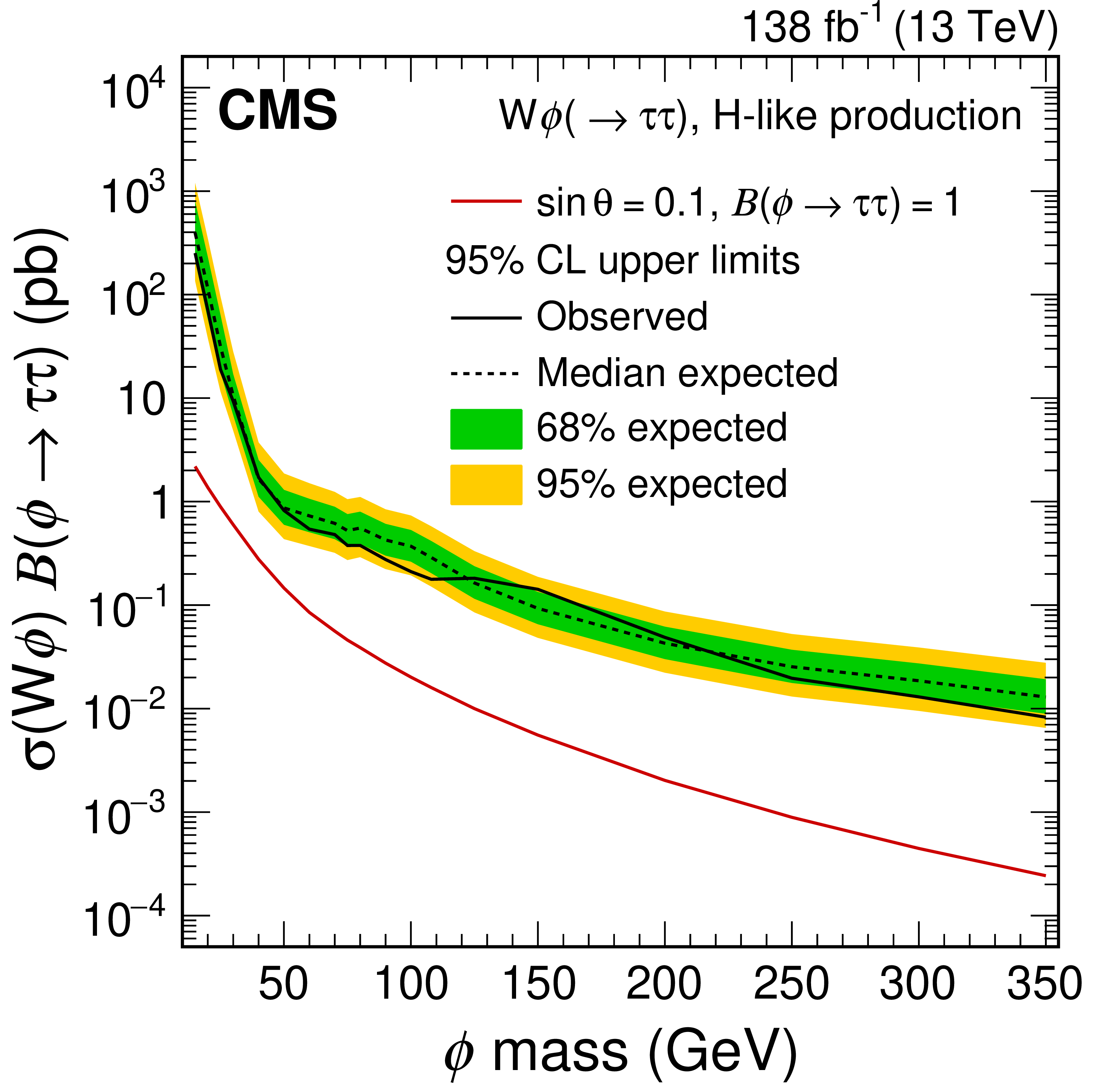
png pdf	Figure 13-e: The 95% confidence level upper limits on the product of the production cross section and branching fraction of the $ {\mathrm{W}}{\phi} $ signal with H-like couplings in the $ \tau\tau $ decay scenario. The vertical gray band indicates the mass region not considered in the analysis. The red line is the theoretical prediction for the product of the production cross section and branching fraction of the $ {\mathrm{W}}{\phi} $ signal.
png pdf	Figure 13-f: The 95% confidence level upper limits on the product of the production cross section and branching fraction of the $ {\mathrm{Z}}{\phi} $ signal with H-like couplings in the $ \tau\tau $ decay scenario. The vertical gray band indicates the mass region not considered in the analysis. The red line is the theoretical prediction for the product of the production cross section and branching fraction of the $ {\mathrm{Z}}{\phi} $ signal.
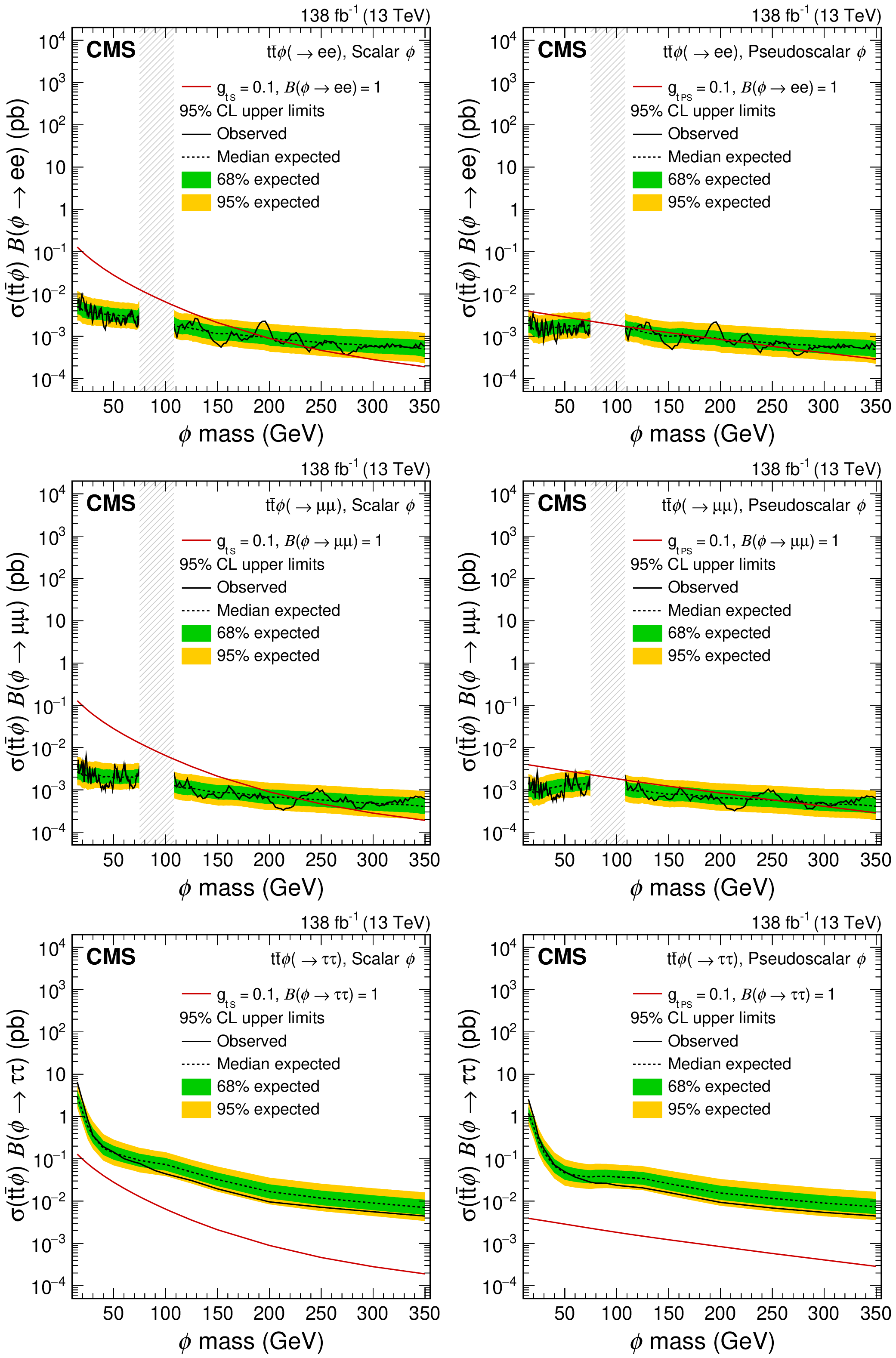
png pdf	Figure 14: The 95% confidence level upper limits on the product of the production cross section and branching fraction of the $ {{\mathrm{t}\overline{\mathrm{t}}} }{\phi} $ signal in the $ \mathrm{e}\mathrm{e} $ (upper), $ \mu\mu $ (middle) and $ \tau\tau $ (lower) decay scenarios. The results for the scalar coupling are shown on the left and pseudoscalar on the right. The vertical gray band indicates the mass region not considered in the analysis. The red line is the theoretical prediction for the product of the production cross section and branching fraction of the $ {{\mathrm{t}\overline{\mathrm{t}}} }{\phi} $ signal.
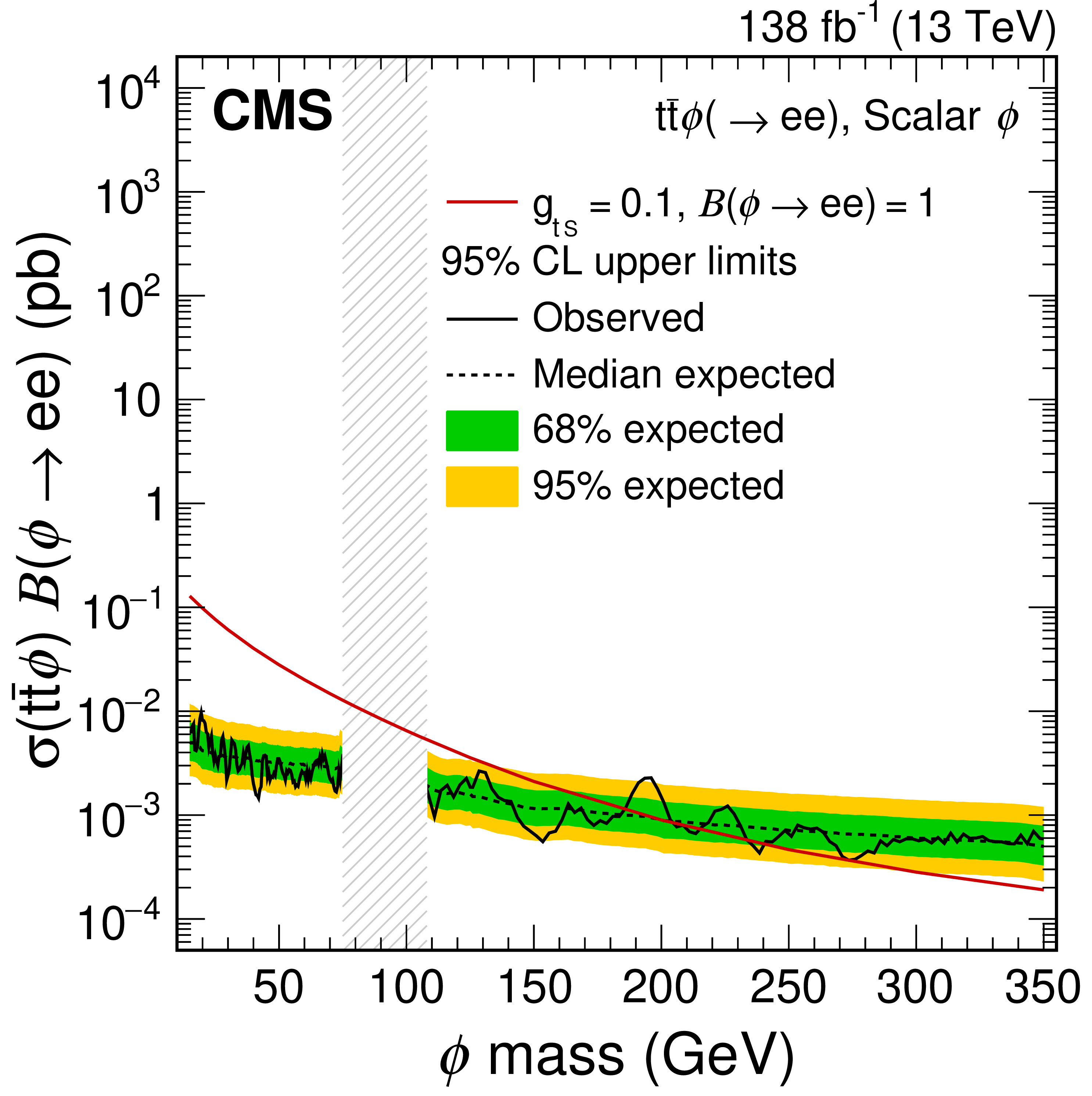
png pdf	Figure 14-a: The 95% confidence level upper limits on the product of the production cross section and branching fraction of the $ {{\mathrm{t}\overline{\mathrm{t}}} }{\phi} $ signal in the $ \mathrm{e}\mathrm{e} $ decay scenario, for the scalar coupling. The vertical gray band indicates the mass region not considered in the analysis. The red line is the theoretical prediction for the product of the production cross section and branching fraction of the $ {{\mathrm{t}\overline{\mathrm{t}}} }{\phi} $ signal.
png pdf	Figure 14-b: The 95% confidence level upper limits on the product of the production cross section and branching fraction of the $ {{\mathrm{t}\overline{\mathrm{t}}} }{\phi} $ signal in the $ \mathrm{e}\mathrm{e} $ decay scenario, for the pseudoscalar coupling. The vertical gray band indicates the mass region not considered in the analysis. The red line is the theoretical prediction for the product of the production cross section and branching fraction of the $ {{\mathrm{t}\overline{\mathrm{t}}} }{\phi} $ signal.
png pdf	Figure 14-c: The 95% confidence level upper limits on the product of the production cross section and branching fraction of the $ {{\mathrm{t}\overline{\mathrm{t}}} }{\phi} $ signal in the $ \mu\mu $ decay scenario, for the scalar coupling. The vertical gray band indicates the mass region not considered in the analysis. The red line is the theoretical prediction for the product of the production cross section and branching fraction of the $ {{\mathrm{t}\overline{\mathrm{t}}} }{\phi} $ signal.
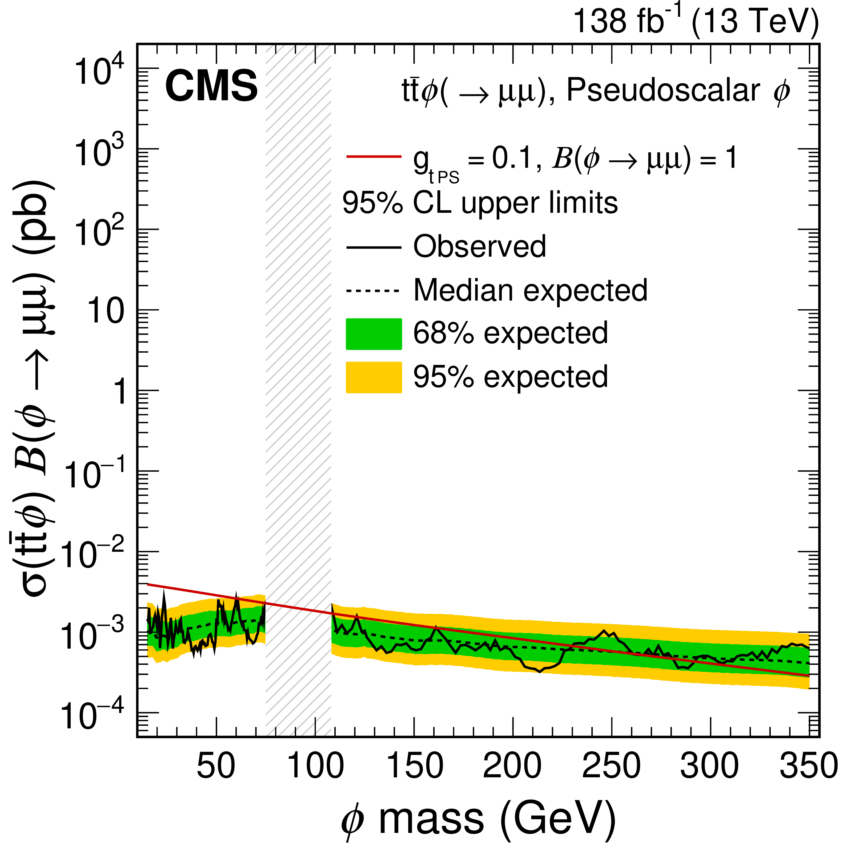
png pdf	Figure 14-d: The 95% confidence level upper limits on the product of the production cross section and branching fraction of the $ {{\mathrm{t}\overline{\mathrm{t}}} }{\phi} $ signal in the $ \mu\mu $ decay scenario, for the pseudoscalar coupling. The vertical gray band indicates the mass region not considered in the analysis. The red line is the theoretical prediction for the product of the production cross section and branching fraction of the $ {{\mathrm{t}\overline{\mathrm{t}}} }{\phi} $ signal.
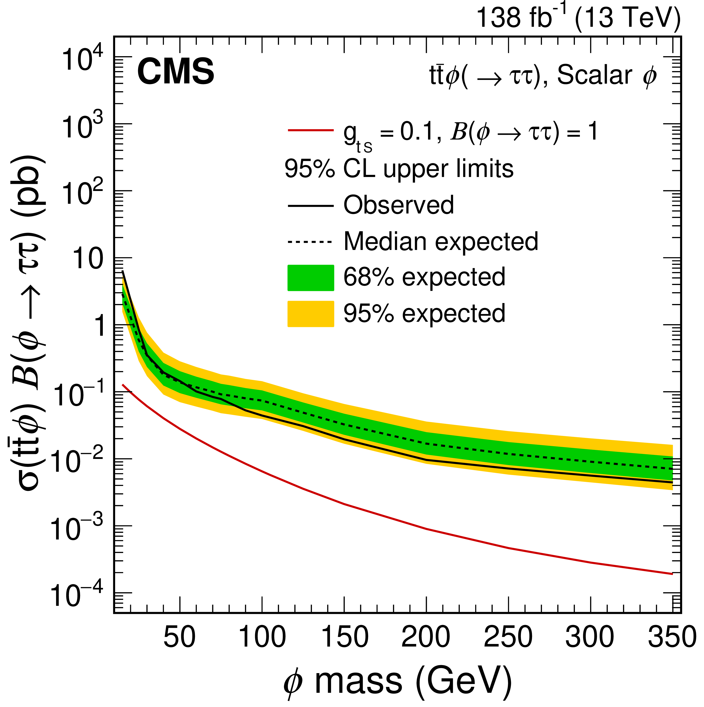
png pdf	Figure 14-e: The 95% confidence level upper limits on the product of the production cross section and branching fraction of the $ {{\mathrm{t}\overline{\mathrm{t}}} }{\phi} $ signal in the $ \tau\tau $ decay scenario, for the scalar coupling. The vertical gray band indicates the mass region not considered in the analysis. The red line is the theoretical prediction for the product of the production cross section and branching fraction of the $ {{\mathrm{t}\overline{\mathrm{t}}} }{\phi} $ signal.
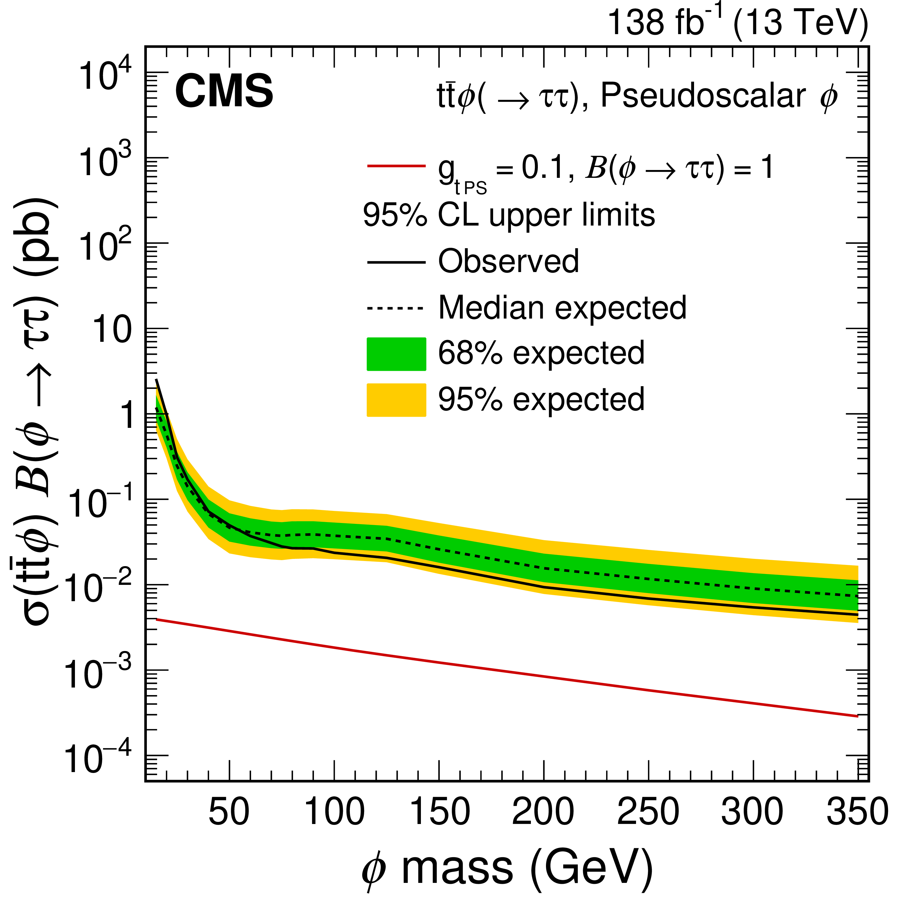
png pdf	Figure 14-f: The 95% confidence level upper limits on the product of the production cross section and branching fraction of the $ {{\mathrm{t}\overline{\mathrm{t}}} }{\phi} $ signal in the $ \tau\tau $ decay scenario, for the pseudoscalar coupling. The vertical gray band indicates the mass region not considered in the analysis. The red line is the theoretical prediction for the product of the production cross section and branching fraction of the $ {{\mathrm{t}\overline{\mathrm{t}}} }{\phi} $ signal.
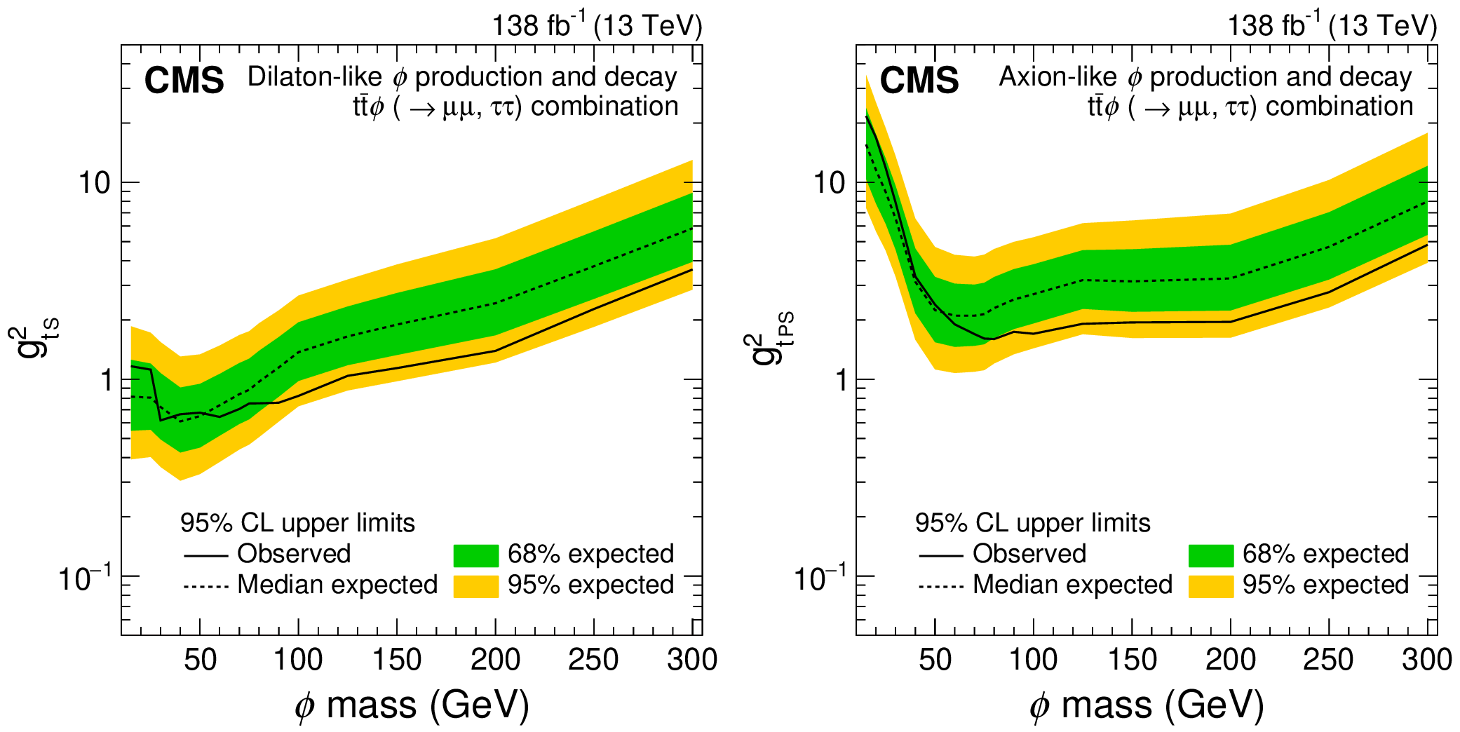
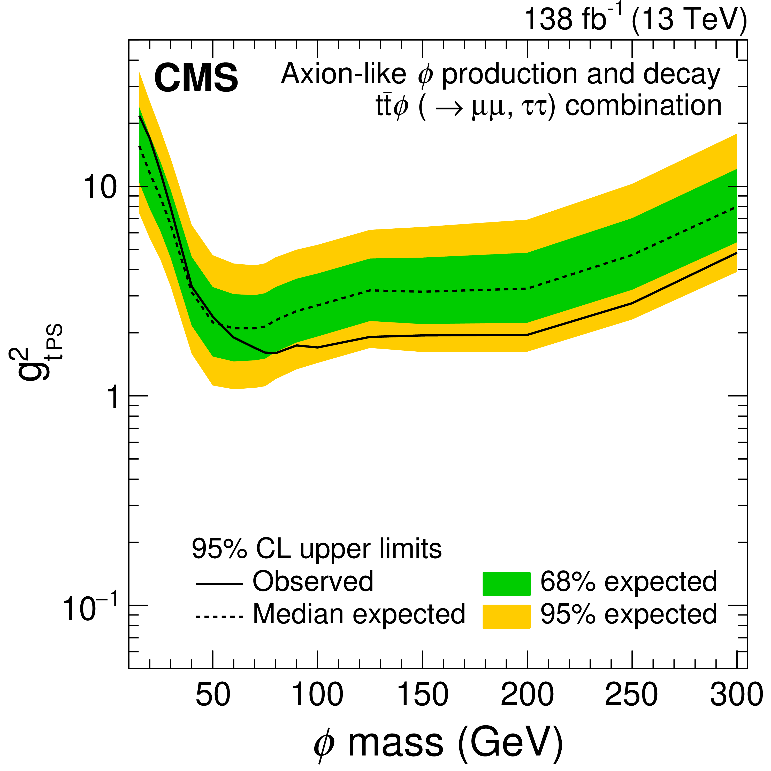
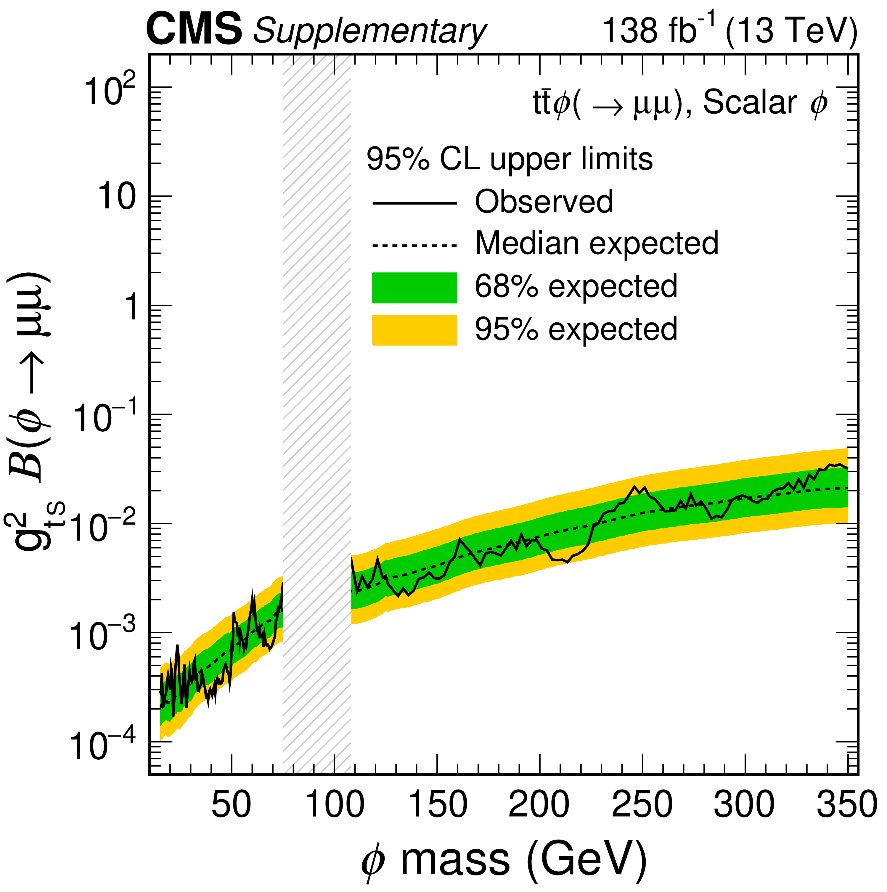
png pdf	Figure 15: The 95% confidence level upper limits on $ {\mathrm{g}}_{{\mathrm{t S}}}^2 $ and $ {\mathrm{g}}_{{\mathrm{t PS}}}^2 $ for the dilaton- and axion-like $ {{\mathrm{t}\overline{\mathrm{t}}} }{\phi} $ signal model (left and right). Masses of the $ \phi $ boson above 300 GeV are not probed for the dilaton- and axion-like signal models as the $ \phi $ branching fraction into top quark-antiquark pairs becomes nonnegligible.
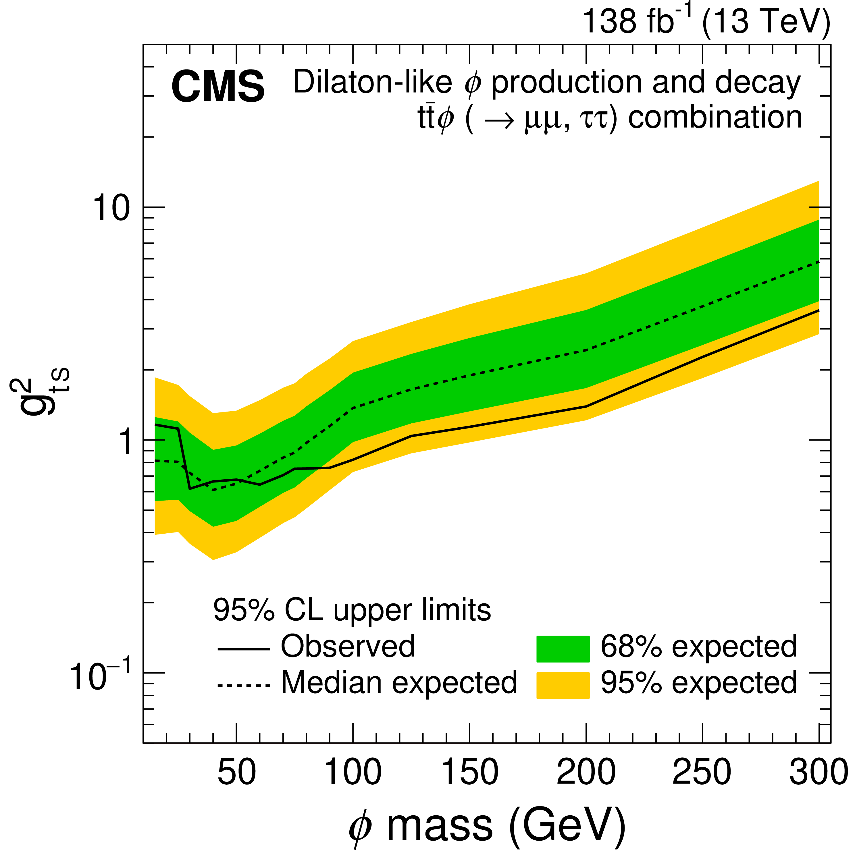
png pdf	Figure 15-a: The 95% confidence level upper limits on $ {\mathrm{g}}_{{\mathrm{t S}}}^2 $ and $ {\mathrm{g}}_{{\mathrm{t PS}}}^2 $ for the dilaton-like $ {{\mathrm{t}\overline{\mathrm{t}}} }{\phi} $ signal model. Masses of the $ \phi $ boson above 300 GeV are not probed for the dilaton-like signal model as the $ \phi $ branching fraction into top quark-antiquark pairs becomes nonnegligible.
png pdf	Figure 15-b: The 95% confidence level upper limits on $ {\mathrm{g}}_{{\mathrm{t S}}}^2 $ and $ {\mathrm{g}}_{{\mathrm{t PS}}}^2 $ for the axion-like $ {{\mathrm{t}\overline{\mathrm{t}}} }{\phi} $ signal model. Masses of the $ \phi $ boson above 300 GeV are not probed for the axion-like signal model as the $ \phi $ branching fraction into top quark-antiquark pairs becomes nonnegligible.
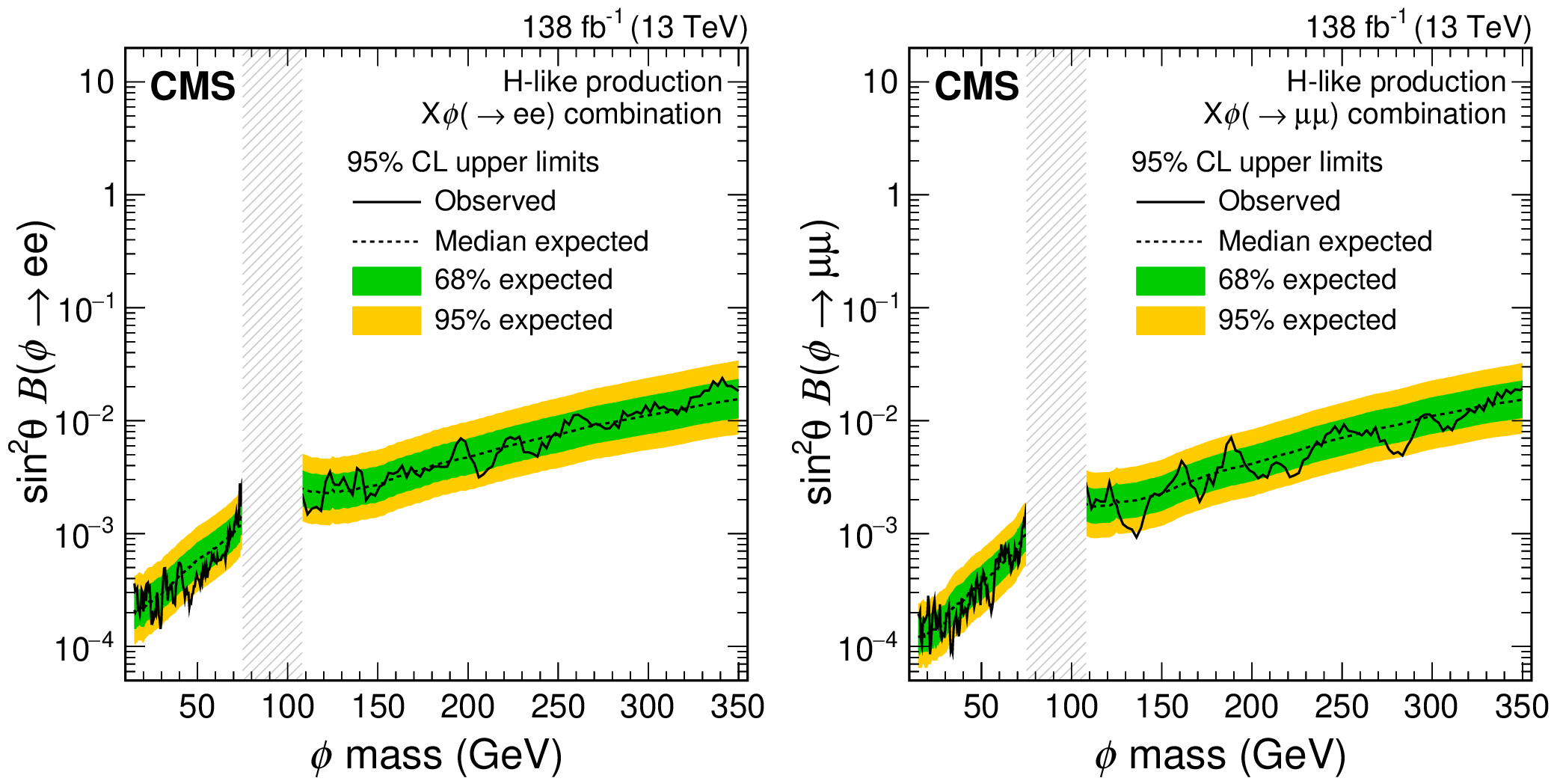
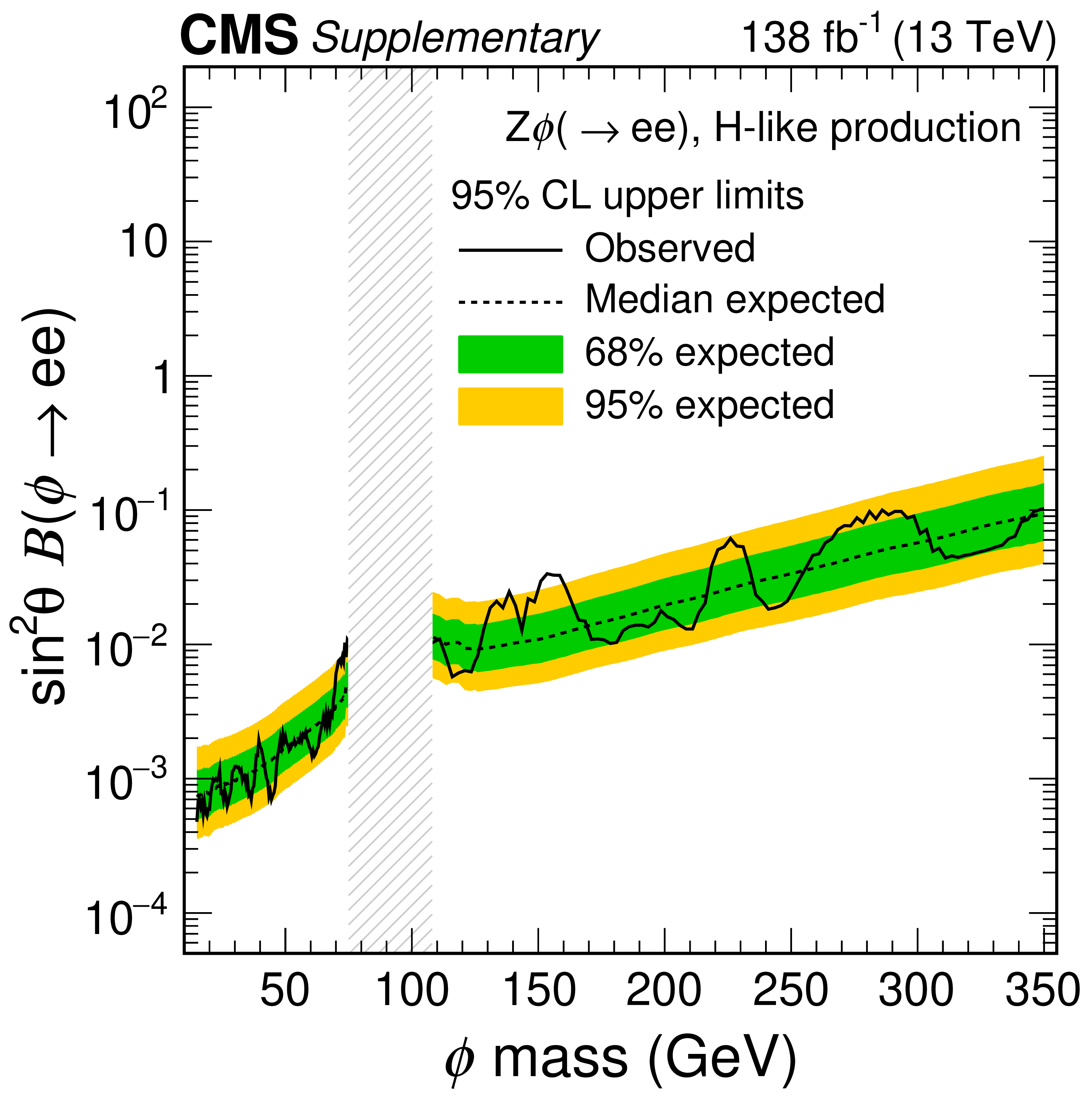
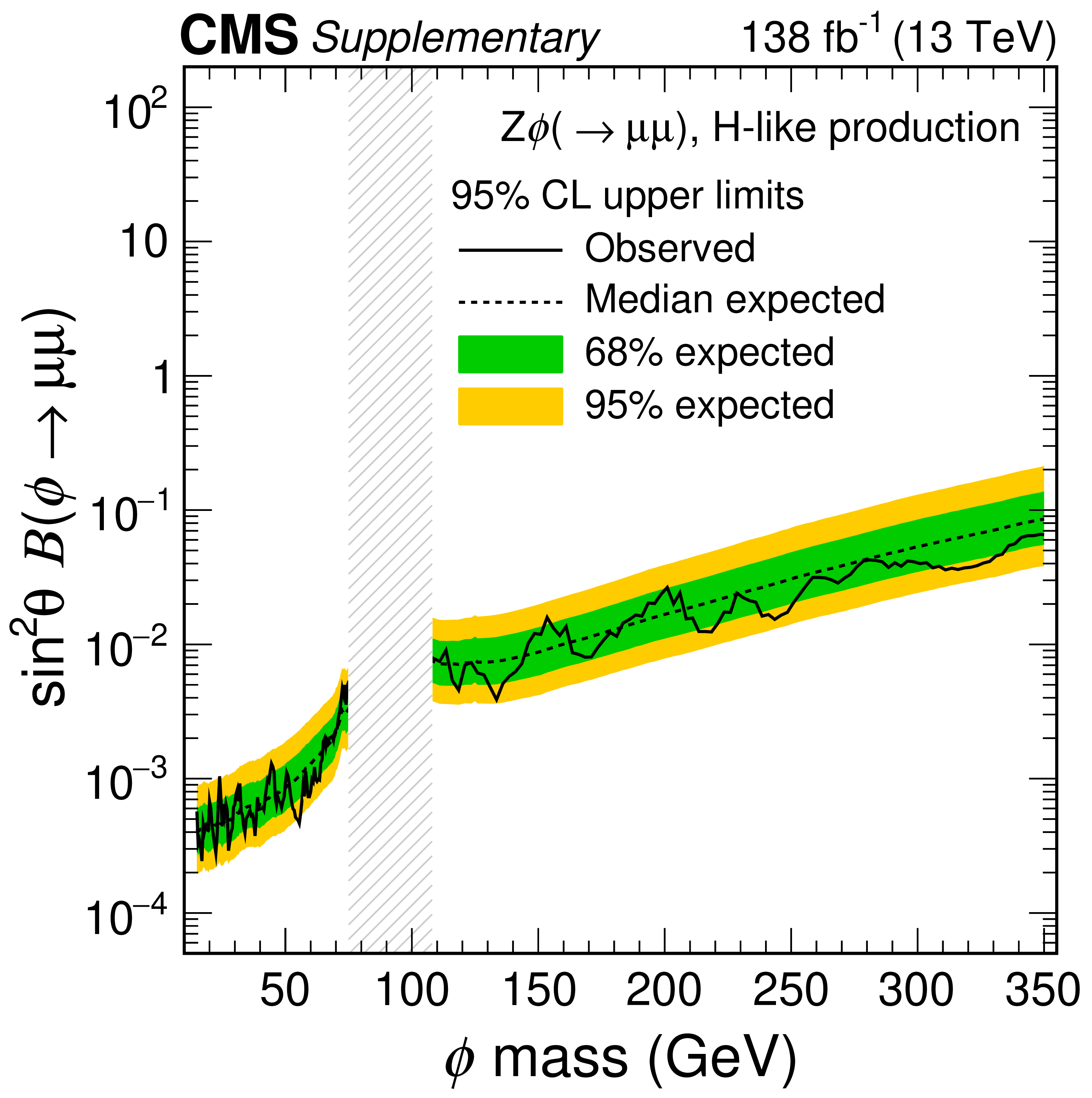
png pdf	Figure 16: The 95% confidence level upper limits on the product of $ \sin^2\theta $ and branching fraction for the H-like production of $ {\mathrm{X}}{\phi}\to\mathrm{e}\mathrm{e} $ and $ {\mathrm{X}}{\phi}\to\mu\mu $ (left and right). The vertical gray band indicates the mass region not considered in the analysis.
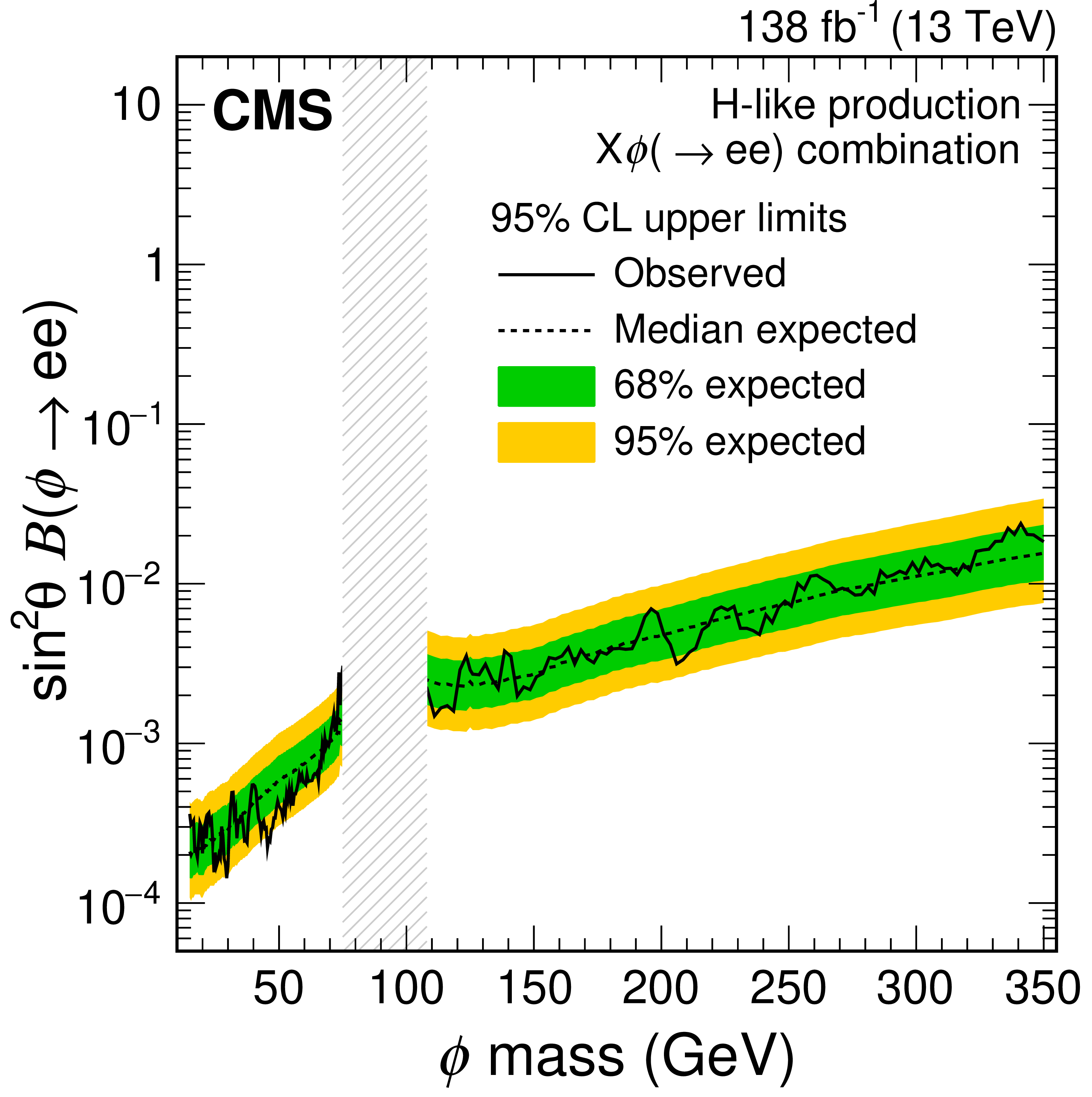
png pdf	Figure 16-a: The 95% confidence level upper limits on the product of $ \sin^2\theta $ and branching fraction for the H-like production of $ {\mathrm{X}}{\phi}\to\mathrm{e}\mathrm{e} $. The vertical gray band indicates the mass region not considered in the analysis.
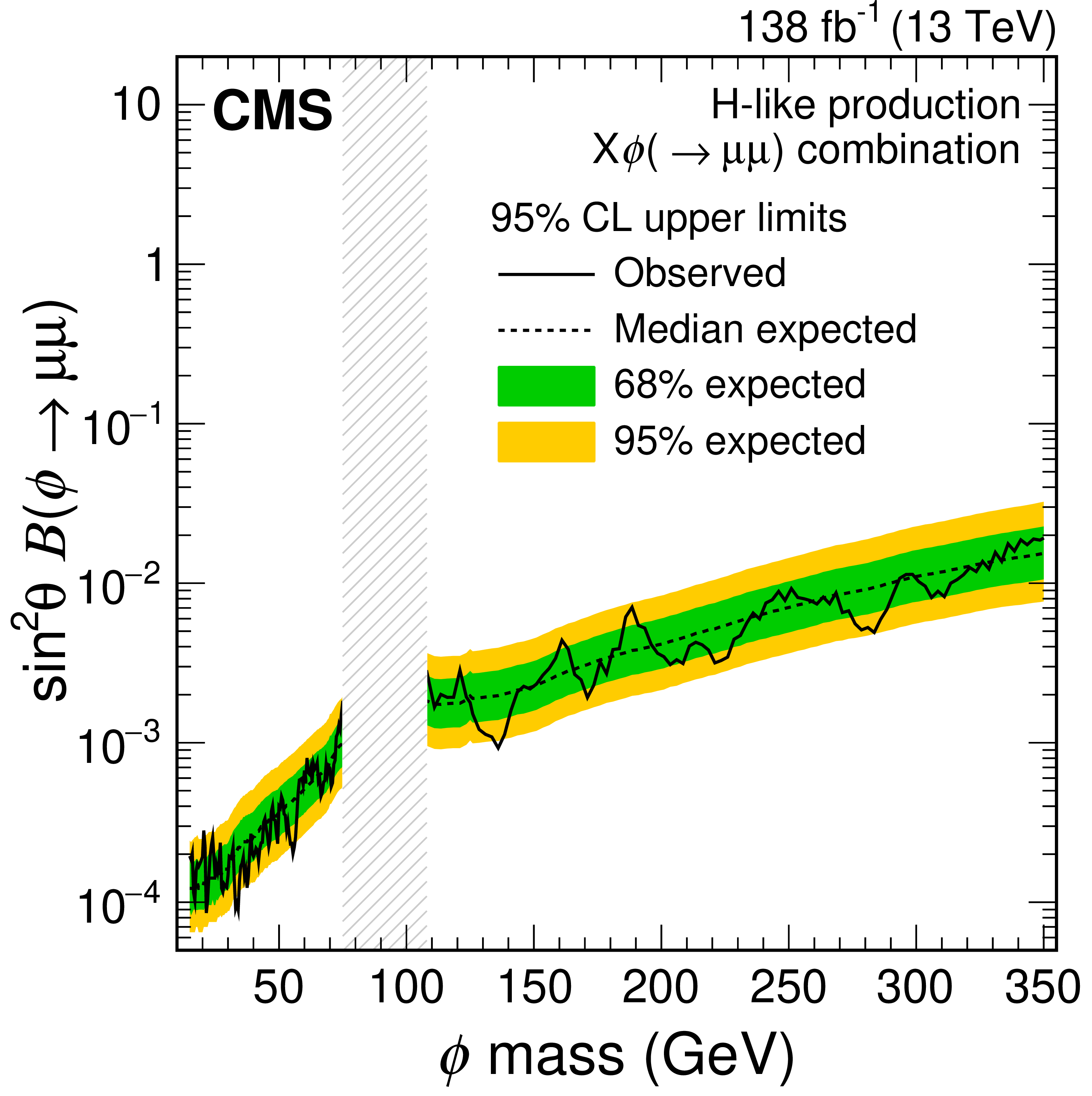
png pdf	Figure 16-b: The 95% confidence level upper limits on the product of $ \sin^2\theta $ and branching fraction for the H-like production of $ {\mathrm{X}}{\phi}\to\mu\mu $. The vertical gray band indicates the mass region not considered in the analysis.
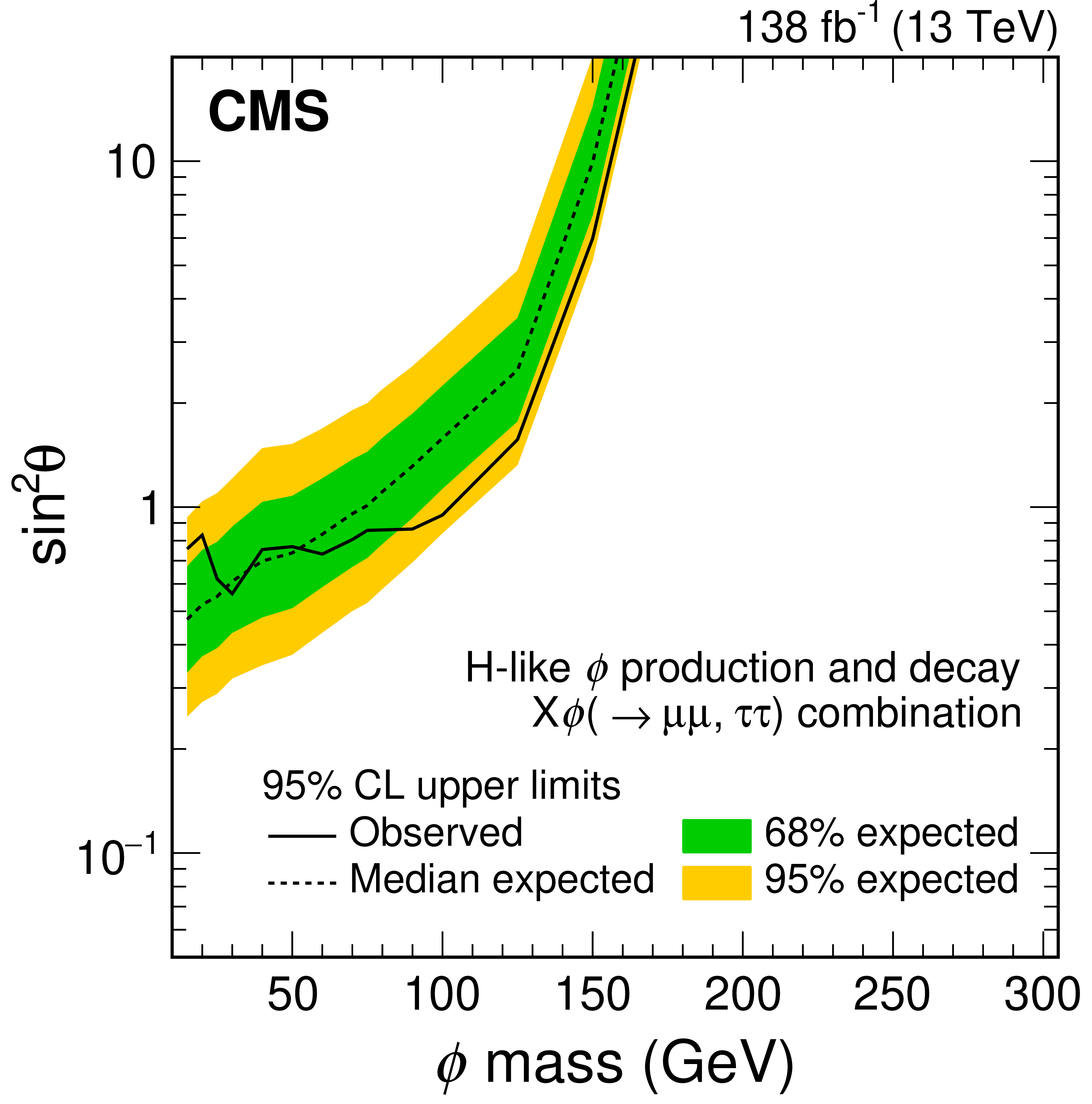
png pdf	Figure 17: The 95% confidence level upper limits on $ \sin^2\theta $ for the H-like production and decay of $ {\mathrm{X}}{\phi} $ signal model.

Tables
png pdf	Table 1: A summary of control regions for the SM processes $ {\mathrm{Z}}{\mathrm{Z}} $, $ {\mathrm{Z}}{\gamma} $, $ {\mathrm{W}}{\mathrm{Z}} $, and $ {{\mathrm{t}\overline{\mathrm{t}}} }{\mathrm{Z}} $, and for the misidentified lepton backgrounds (MisID $ \mathrm{e}/\mu $ and MisID $ \tau $). The $ p_{\mathrm{T}}^\text{miss} $, $ M_{\mathrm{T}} $, 3L minimum lepton transverse momentum $ p_{\mathrm{T3}} $, $ M_{\ell} $, and $ S_{\mathrm{T}} $ quantities are given in units of GeV. The 3L OnZ CR is further split into 3L MisID $ \mathrm{e}/\mu $ CR, 3L $ {\mathrm{W}}{\mathrm{Z}} $ CR, and 3L $ {{\mathrm{t}\overline{\mathrm{t}}} }{\mathrm{Z}} $ CR. The terminology is described in Section 5.
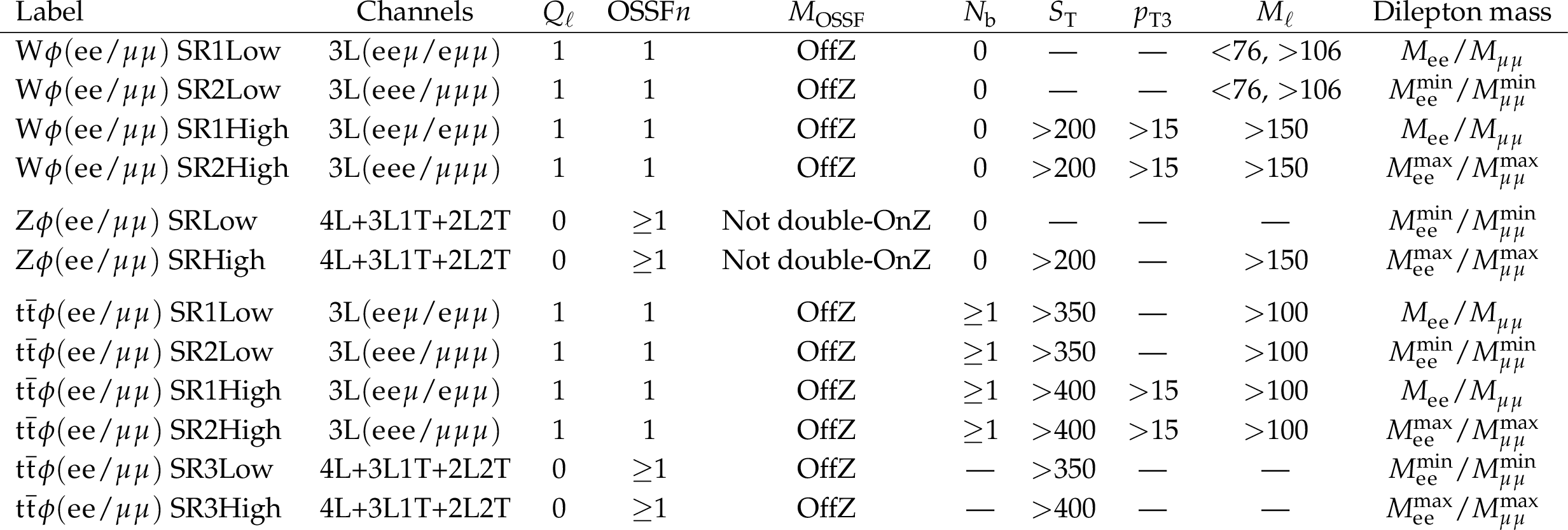
png pdf	Table 2: Low- and high-mass signal region selections for $ {\mathrm{X}}{\phi}\to\mathrm{e}\mathrm{e}/\mu\mu $ signals. Events satisfying the control region requirements are vetoed throughout, and only those with a reconstructed $ \phi $ candidate are retained using the specified dilepton mass variable. The $ S_{\mathrm{T}} $, $ p_{\mathrm{T3}} $, and $ M_{\ell} $ requirements are specified in units of GeV. The two entries in the labels, channels, and dilepton mass variables are provided for the $ X\phi\to\mathrm{e}\mathrm{e} $ and $ X\phi\to\mu\mu $ signal scenarios, as appropriate.
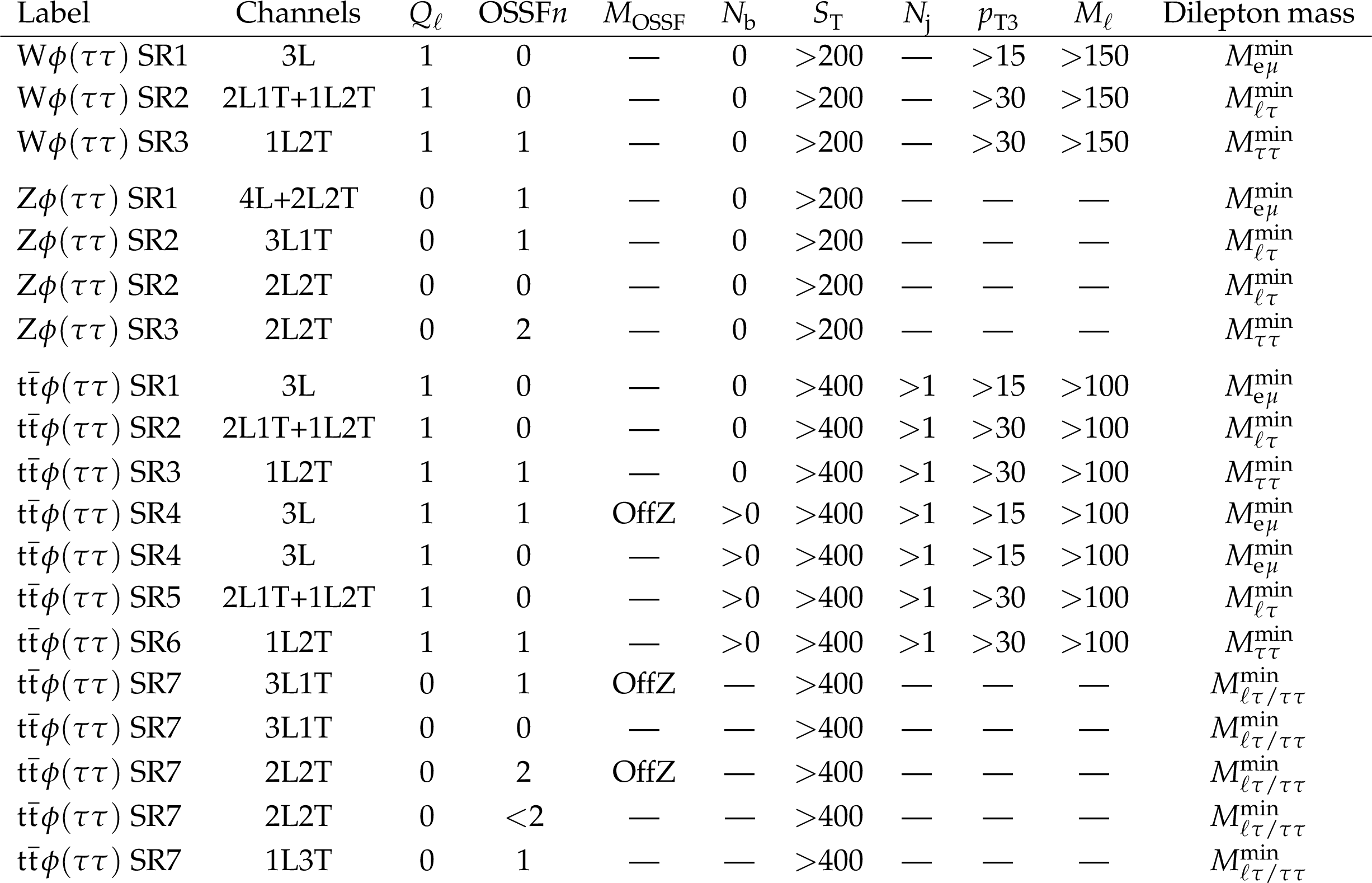
png pdf	Table 3: Signal selections for $ {\mathrm{X}}{\phi}\to\tau\tau $ signals. Events satisfying the control region requirements are vetoed throughout, and only those with a reconstructed $ \phi $ candidate are retained using the specified dilepton mass variable. The $ S_{\mathrm{T}} $, $ p_{\mathrm{T3}} $, and $ M_{\ell} $ requirements are specified in units of GeV.
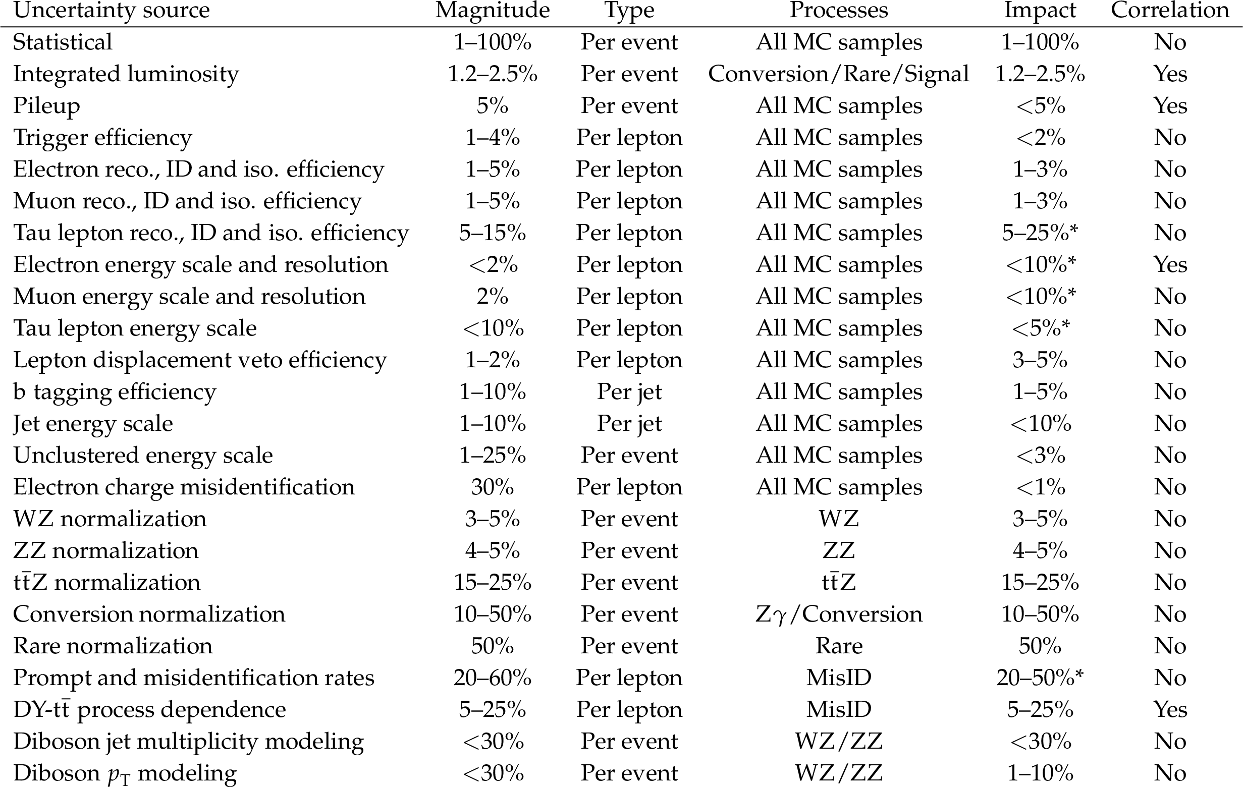
png pdf	Table 4: Sources, magnitudes, impacts, and correlation properties of systematic uncertainties in the signal regions. Magnitude refers to the relative change in the underlying uncertainty source, whereas impact quantifies the resultant relative change in the signal and background yields passing the event selection. Uncertainty sources marked as ``Yes'' under the Correlation column are correlated across the 3 years of data collection, and those marked with an asterisk in the Impact column are mass-dependent.
png pdf	Table 5: A summary of model-dependent scenarios, and the corresponding subsets of SRs combined in the interpretations.

Summary

A search for beyond-the-standard-model phenomena producing resonant dilepton signatures of any flavor in multilepton events has been performed using pp collision data collected with the CMS detector at $ \sqrt{s} = $ 13 TeV, corresponding to an integrated luminosity of 138 fb$ ^{-1} $. The results provide direct and model independent constraints on the allowed parameter space for new spin-0 particles, $ \phi $, with scalar, pseudoscalar, or H-like couplings. The $ \phi $ bosons are assumed to be produced in association with a W or Z boson or a top quark-antiquark ($ \mathrm{t} \overline{\mathrm{t}} $) pair, and decay into $ \mathrm{e}\mathrm{e} $, $ \mu\mu $, or $ \tau\tau $ pairs. Constraints are calculated at 95% confidence level on the product of the production cross section and leptonic branching fraction of such bosons with masses in the range 15-350 GeV. No statistically significant excess is observed over the standard model background in the probed mass spectra. Over this mass range, the product of the cross section and branching fraction for the $ \tau\tau $ ($ \mathrm{e}\mathrm{e} $ and $ \mu\mu $) final states is excluded above 0.004-35, 0.004-80, and 0.008-250 pb (0.5-50, 0.5-30, and 1-200 fb) as a function of $ \phi $ mass for scalar, pseudoscalar, and H-like bosons, respectively. Several model-dependent interpretations have also been considered. The $ {{\mathrm{t}\overline{\mathrm{t}}} }{\phi} $ mode provides the first direct bounds on the coupling of the $ \phi $ boson to top quarks in the context of fermiophilic models. For a fermiophilic dilaton-like model with scalar couplings, the most stringent limit on the coupling is 0.63-0.66, obtained in the $ \phi $ mass range 40-60 GeV. For a fermiophilic axion-like model with pseudoscalar couplings, the most stringent limit on the coupling is 1.59, obtained for a $ \phi $ mass of 70 GeV. To constrain the Higgs-$ \phi $ mixing angle, $ \sin^2\theta $, in the case where the $ \phi $ is H-like, the independent $ {\mathrm{W}}{\phi} $, $ {\mathrm{Z}}{\phi} $, and $ {{\mathrm{t}\overline{\mathrm{t}}} }{\phi} $ signal regions are combined. The observed (expected) upper limit on $ \sin^2\theta $ is 1.2 (1.9) for a $ \phi $ mass of 125 GeV; the most stringent observed exclusion is obtained for a $ \phi $ mass of 30 GeV, corresponding to an upper limit on $ \sin^2\theta $ of 0.59 (0.64).

Additional Figures
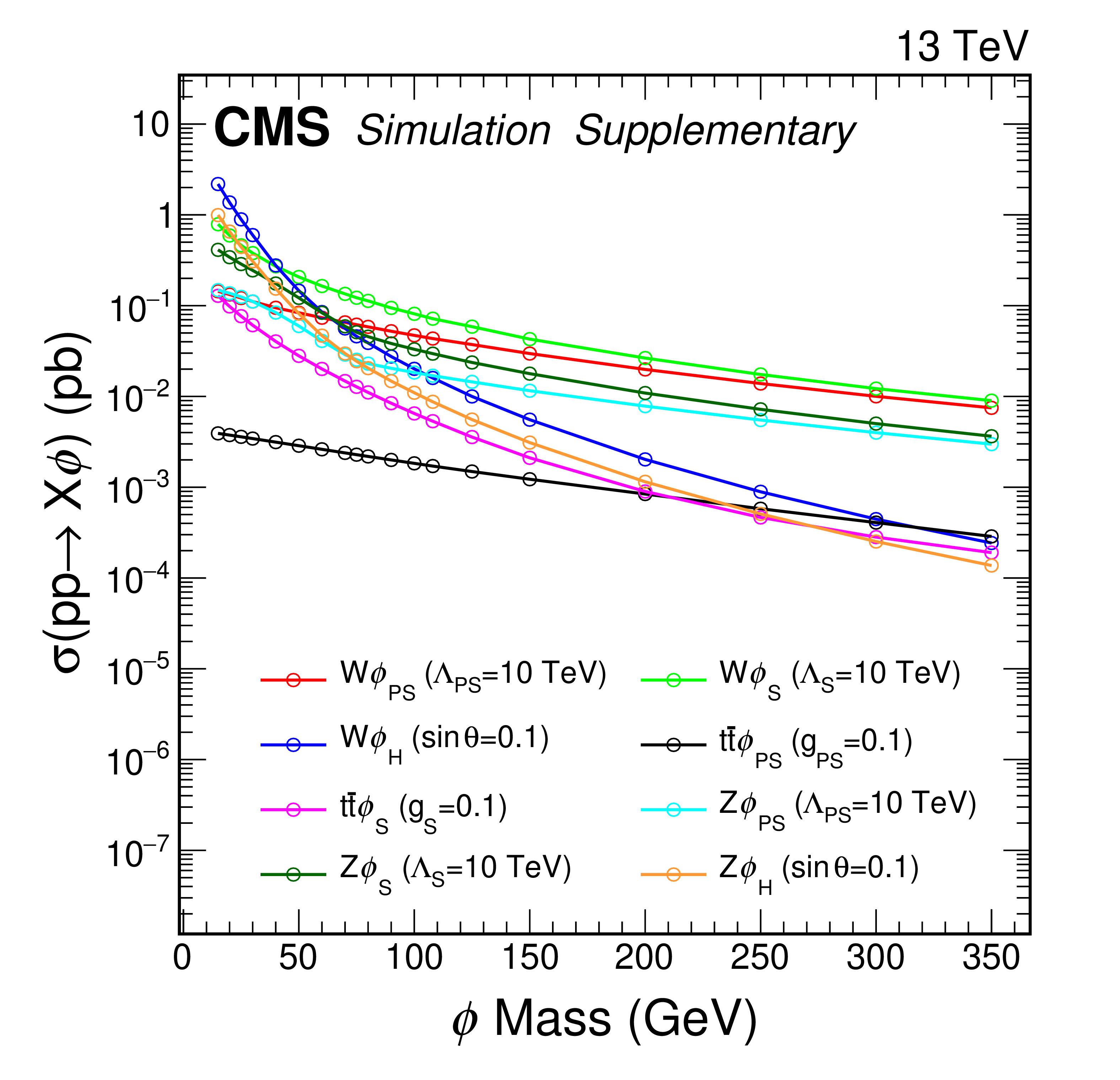
png pdf	Additional Figure 1: Cross section in units of pb for the $ {\mathrm{W}}{\phi} $, $ {\mathrm{Z}}{\phi} $, and $ {{\mathrm{t}\overline{\mathrm{t}}} }{\phi} $ signals as a function of the $ \phi $ boson mass in GeV. All cross sections are inclusive of all W, Z, $ {\mathrm{t}\overline{\mathrm{t}}} $ and $ \phi $ decay modes.
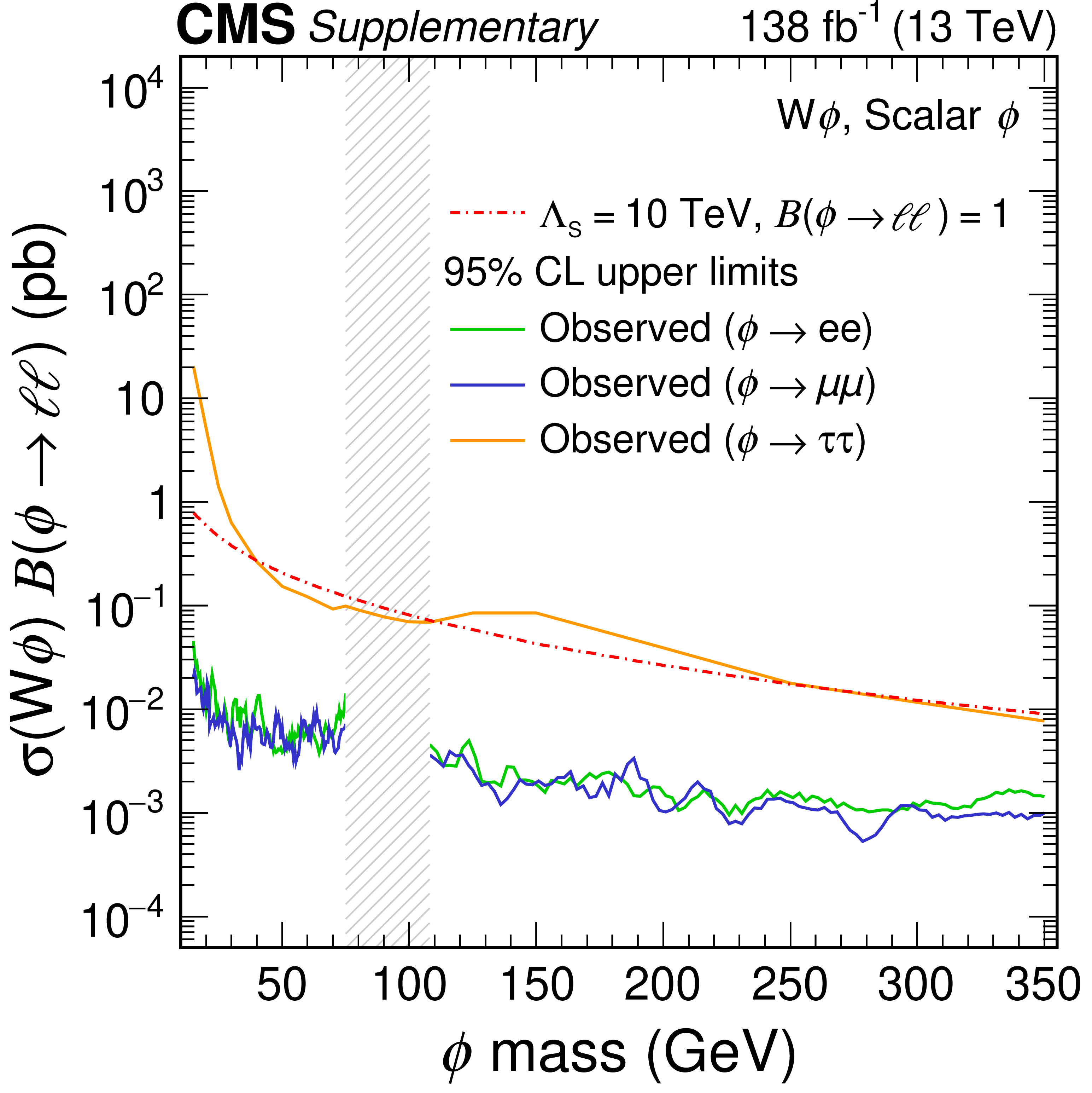
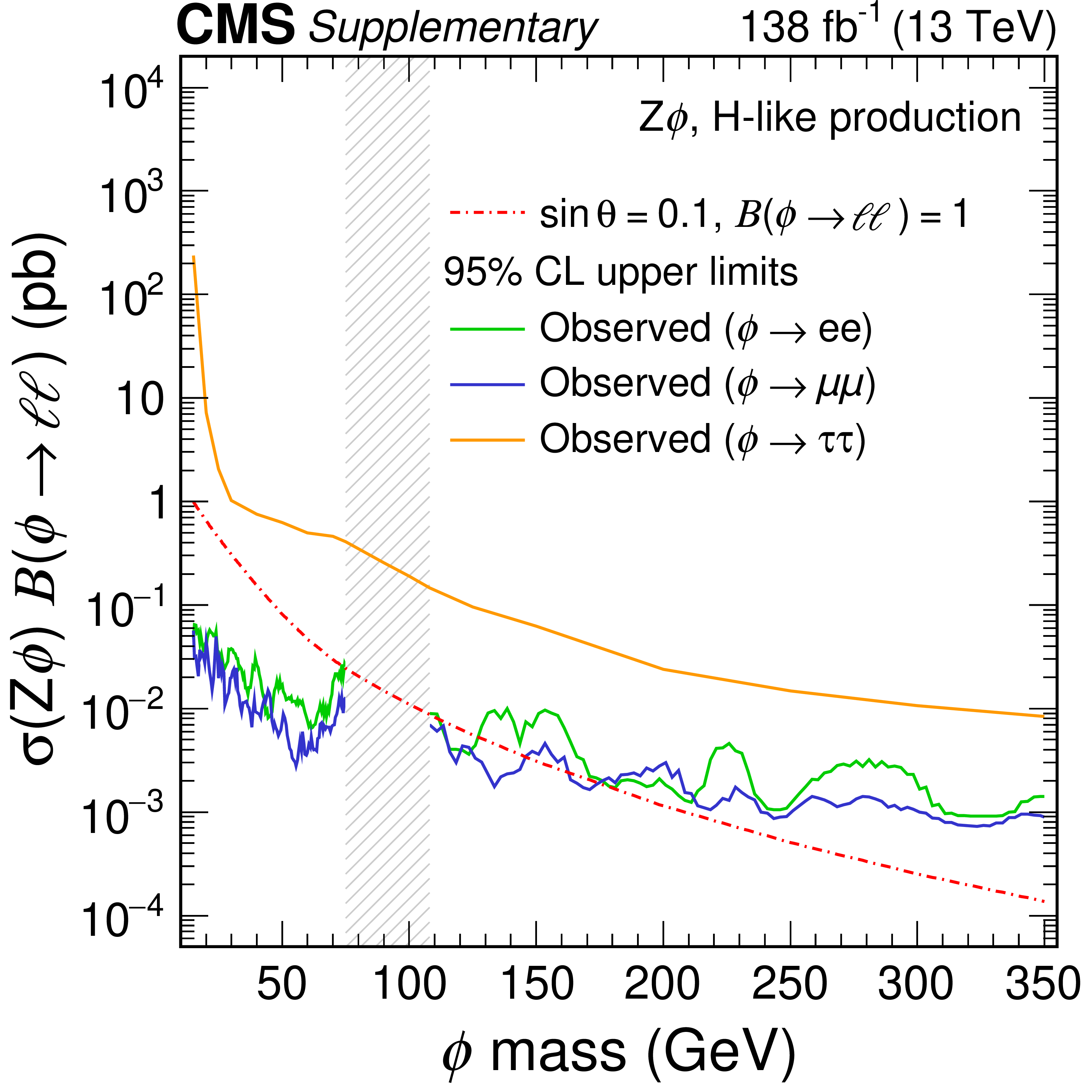
png pdf	Additional Figure 2: The 95% confidence level observed upper limits on the product of $ \sigma({\mathrm{W}}{\phi}) $ and $ \mathcal{B}(\phi \to \ell\ell) $ for the $ {\mathrm{W}}{\phi} $ signal with scalar couplings, where $ \sigma $ denotes the production cross section and $ \mathcal{B}(\phi \to \ell\ell) $ is the branching fraction of the $ \phi $ boson into a lepton pair of given flavor. Exclusions on the dielectron, dimuon, and ditau decay scenarios of the $ \phi $ boson are shown with the green, blue, and orange solid lines, respectively. The red dash-dotted line is the theoretical prediction for $ \sigma\mathcal{B} $ of the $ {\mathrm{W}}{\phi} $ signal. The vertical gray band indicates the mass region not considered in the analysis in the dielectron and dimuon decay scenarios of the $ \phi $ boson.
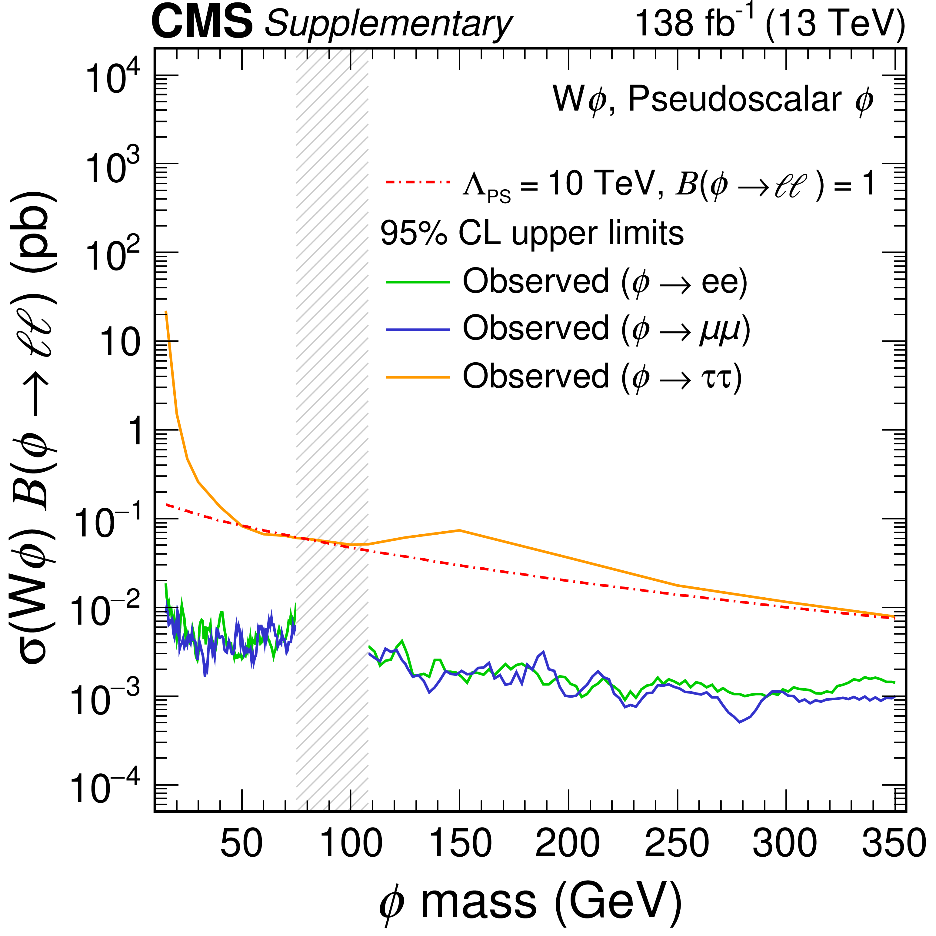
png pdf	Additional Figure 3: The 95% confidence level observed upper limits on the product of $ \sigma({\mathrm{W}}{\phi}) $ and $ \mathcal{B}(\phi \to \ell\ell) $ for the $ {\mathrm{W}}{\phi} $ signal with pseudoscalar couplings, where $ \sigma $ denotes the production cross section and $ \mathcal{B}(\phi \to \ell\ell) $ is the branching fraction of the $ \phi $ boson into a lepton pair of given flavor. Exclusions on the dielectron, dimuon, and ditau decay scenarios of the $ \phi $ boson are shown with the green, blue, and orange solid lines, respectively. The red dash-dotted line is the theoretical prediction for $ \sigma\mathcal{B} $ of the $ {\mathrm{W}}{\phi} $ signal. The vertical gray band indicates the mass region not considered in the analysis in the dielectron and dimuon decay scenarios of the $ \phi $ boson.
png pdf	Additional Figure 4: The 95% confidence level observed upper limits on the product of $ \sigma({\mathrm{W}}{\phi}) $ and $ \mathcal{B}(\phi \to \ell\ell) $ for the $ {\mathrm{W}}{\phi} $ signal with H-like production, where $ \sigma $ denotes the production cross section and $ \mathcal{B}(\phi \to \ell\ell) $ is the branching fraction of the $ \phi $ boson into a lepton pair of given flavor. Exclusions on the dielectron, dimuon, and ditau decay scenarios of the $ \phi $ boson are shown with the green, blue, and orange solid lines, respectively. The red dash-dotted line is the theoretical prediction for $ \sigma\mathcal{B} $ of the $ {\mathrm{W}}{\phi} $ signal. The vertical gray band indicates the mass region not considered in the analysis in the dielectron and dimuon decay scenarios of the $ \phi $ boson.
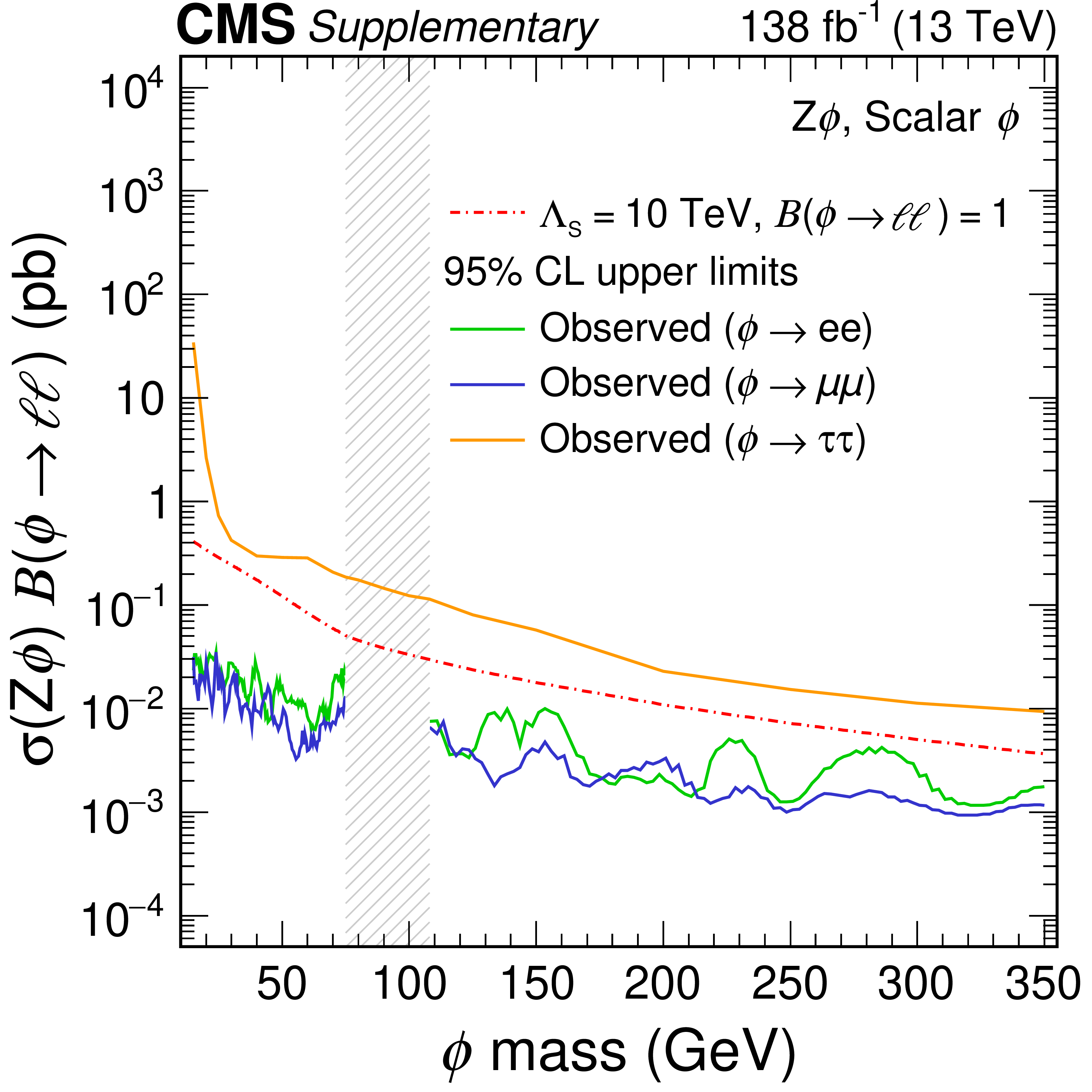
png pdf	Additional Figure 5: The 95% confidence level observed upper limits on the product of $ \sigma({\mathrm{Z}}{\phi}) $ and $ \mathcal{B}(\phi \to \ell\ell) $ for the $ {\mathrm{Z}}{\phi} $ signal with scalar couplings, where $ \sigma $ denotes the production cross section and $ \mathcal{B}(\phi \to \ell\ell) $ is the branching fraction of the $ \phi $ boson into a lepton pair of given flavor. Exclusions on the dielectron, dimuon, and ditau decay scenarios of the $ \phi $ boson are shown with the green, blue, and orange solid lines, respectively. The red dash-dotted line is the theoretical prediction for $ \sigma\mathcal{B} $ of the $ {\mathrm{Z}}{\phi} $ signal. The vertical gray band indicates the mass region not considered in the analysis in the dielectron and dimuon decay scenarios of the $ \phi $ boson.
png pdf	Additional Figure 6: The 95% confidence level observed upper limits on the product of $ \sigma({\mathrm{Z}}{\phi}) $ and $ \mathcal{B}(\phi \to \ell\ell) $ for the $ {\mathrm{Z}}{\phi} $ signal with pseudoscalar couplings, where $ \sigma $ denotes the production cross section and $ \mathcal{B}(\phi \to \ell\ell) $ is the branching fraction of the $ \phi $ boson into a lepton pair of given flavor. Exclusions on the dielectron, dimuon, and ditau decay scenarios of the $ \phi $ boson are shown with the green, blue, and orange solid lines, respectively. The red dash-dotted line is the theoretical prediction for $ \sigma\mathcal{B} $ of the $ {\mathrm{Z}}{\phi} $ signal. The vertical gray band indicates the mass region not considered in the analysis in the dielectron and dimuon decay scenarios of the $ \phi $ boson.
png pdf	Additional Figure 7: The 95% confidence level observed upper limits on the product of $ \sigma({\mathrm{Z}}{\phi}) $ and $ \mathcal{B}(\phi \to \ell\ell) $ for the $ {\mathrm{Z}}{\phi} $ signal with H-like production, where $ \sigma $ denotes the production cross section and $ \mathcal{B}(\phi \to \ell\ell) $ is the branching fraction of the $ \phi $ boson into a lepton pair of given flavor. Exclusions on the dielectron, dimuon, and ditau decay scenarios of the $ \phi $ boson are shown with the green, blue, and orange solid lines, respectively. The red dash-dotted line is the theoretical prediction for $ \sigma\mathcal{B} $ of the $ {\mathrm{Z}}{\phi} $ signal. The vertical gray band indicates the mass region not considered in the analysis in the dielectron and dimuon decay scenarios of the $ \phi $ boson.
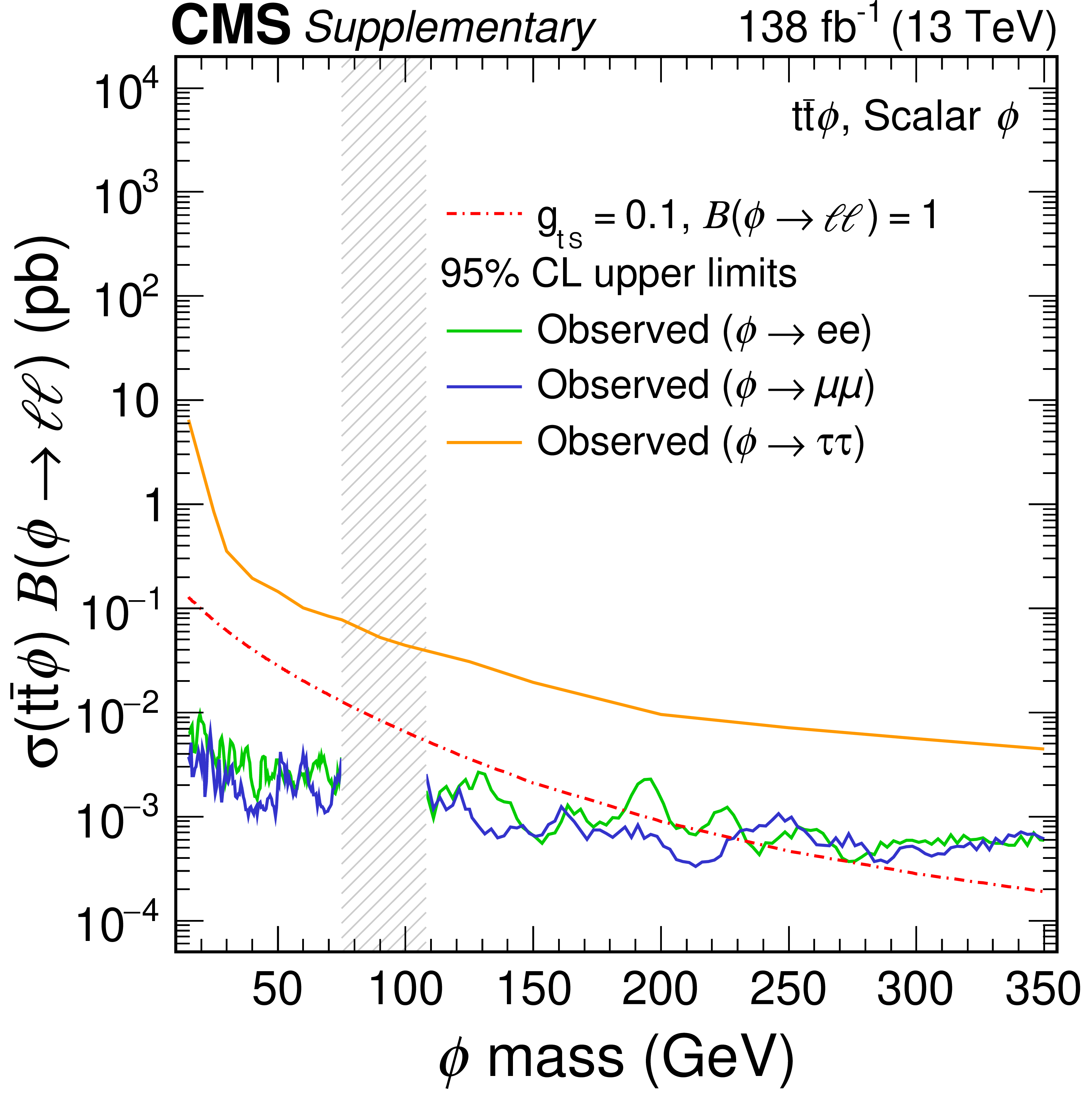
png pdf	Additional Figure 8: The 95% confidence level observed upper limits on the product of $ \sigma({{\mathrm{t}\overline{\mathrm{t}}} }{\phi}) $ and $ \mathcal{B}(\phi \to \ell\ell) $ for the $ {{\mathrm{t}\overline{\mathrm{t}}} }{\phi} $ signal with scalar couplings, where $ \sigma $ denotes the production cross section and $ \mathcal{B}(\phi \to \ell\ell) $ is the branching fraction of the $ \phi $ boson into a lepton pair of given flavor. Exclusions on the dielectron, dimuon, and ditau decay scenarios of the $ \phi $ boson are shown with the green, blue, and orange solid lines, respectively. The red dash-dotted line is the theoretical prediction for $ \sigma\mathcal{B} $ of the $ {{\mathrm{t}\overline{\mathrm{t}}} }{\phi} $ signal. The vertical gray band indicates the mass region not considered in the analysis in the dielectron and dimuon decay scenarios of the $ \phi $ boson.
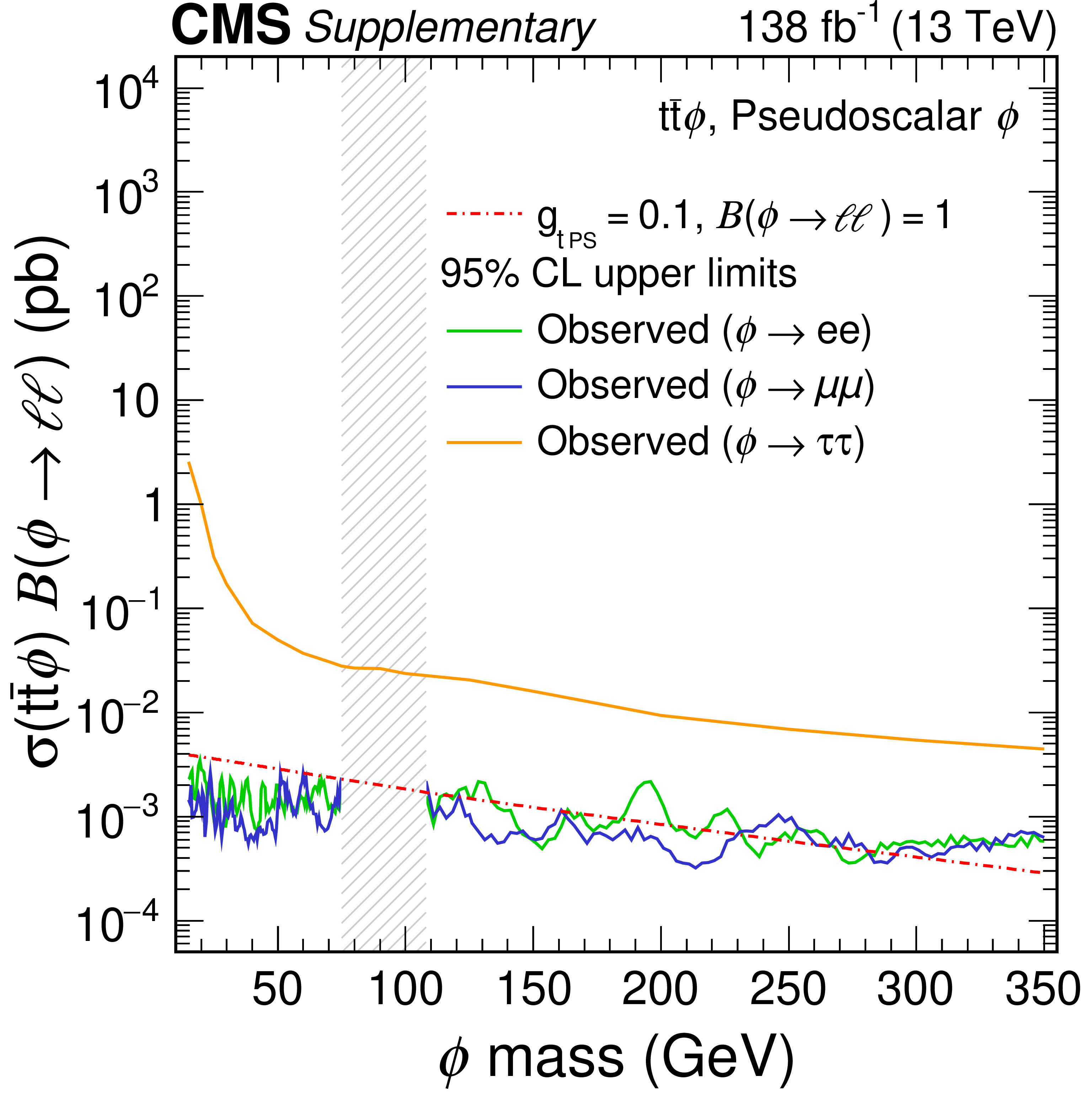
png pdf	Additional Figure 9: The 95% confidence level observed upper limits on the product of $ \sigma({{\mathrm{t}\overline{\mathrm{t}}} }{\phi}) $ and $ \mathcal{B}(\phi \to \ell\ell) $ for the $ {{\mathrm{t}\overline{\mathrm{t}}} }{\phi} $ signal with pseudoscalar couplings, where $ \sigma $ denotes the production cross section and $ \mathcal{B}(\phi \to \ell\ell) $ is the branching fraction of the $ \phi $ boson into a lepton pair of given flavor. Exclusions on the dielectron, dimuon, and ditau decay scenarios of the $ \phi $ boson are shown with the green, blue, and orange solid lines, respectively. The red dash-dotted line is the theoretical prediction for $ \sigma\mathcal{B} $ of the $ {{\mathrm{t}\overline{\mathrm{t}}} }{\phi} $ signal. The vertical gray band indicates the mass region not considered in the analysis in the dielectron and dimuon decay scenarios of the $ \phi $ boson.
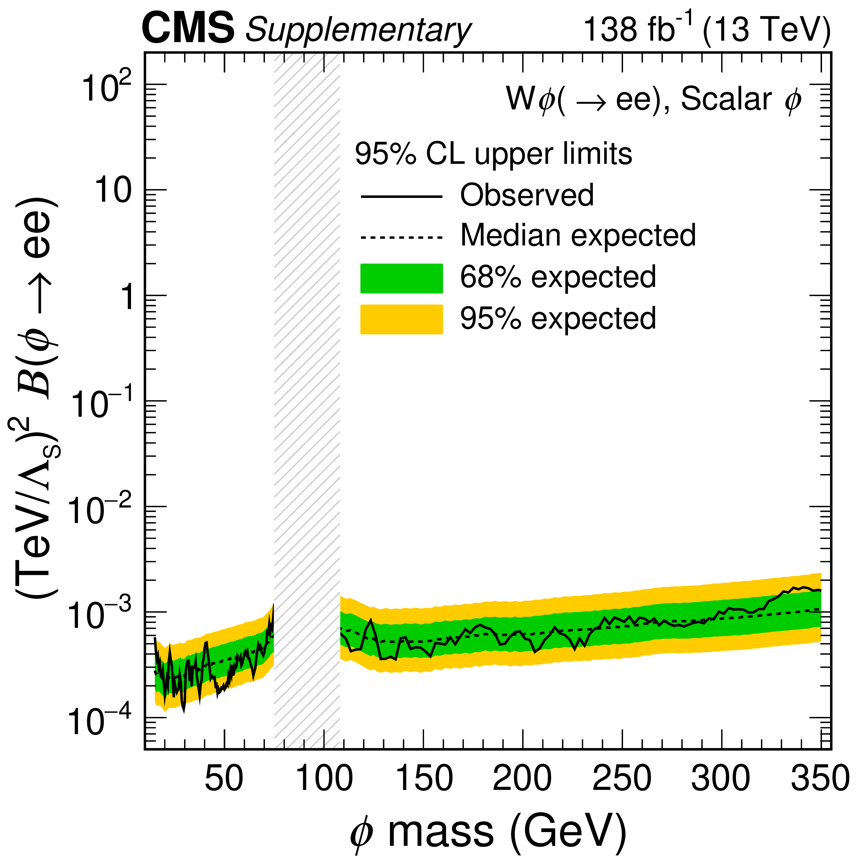
png pdf	Additional Figure 10: The 95% confidence level expected and observed upper limits on the product of $ (1/\Lambda_{\mathrm{S}})^2 $ and $ \mathcal{B}(\phi \to \mathrm{e}\mathrm{e}) $ of the $ {\mathrm{W}}{\phi} $ signal with scalar couplings, where $ \Lambda_{\mathrm{S}} $ denotes the mass scale of the effective interaction and $ \mathcal{B}(\phi \to \mathrm{e}\mathrm{e}) $ is the branching fraction of the $ \phi $ boson into an electron pair. The vertical gray band indicates the mass region not considered in the analysis.
png pdf	Additional Figure 11: The 95% confidence level expected and observed upper limits on the product of $ (1/\Lambda_{\mathrm{S}})^2 $ and $ \mathcal{B}(\phi \to \mu\mu) $ of the $ {\mathrm{W}}{\phi} $ signal with scalar couplings, where $ \Lambda_{\mathrm{S}} $ denotes the mass scale of the effective interaction and $ \mathcal{B}(\phi \to \mu\mu) $ is the branching fraction of the $ \phi $ boson into a muon pair. The vertical gray band indicates the mass region not considered in the analysis.
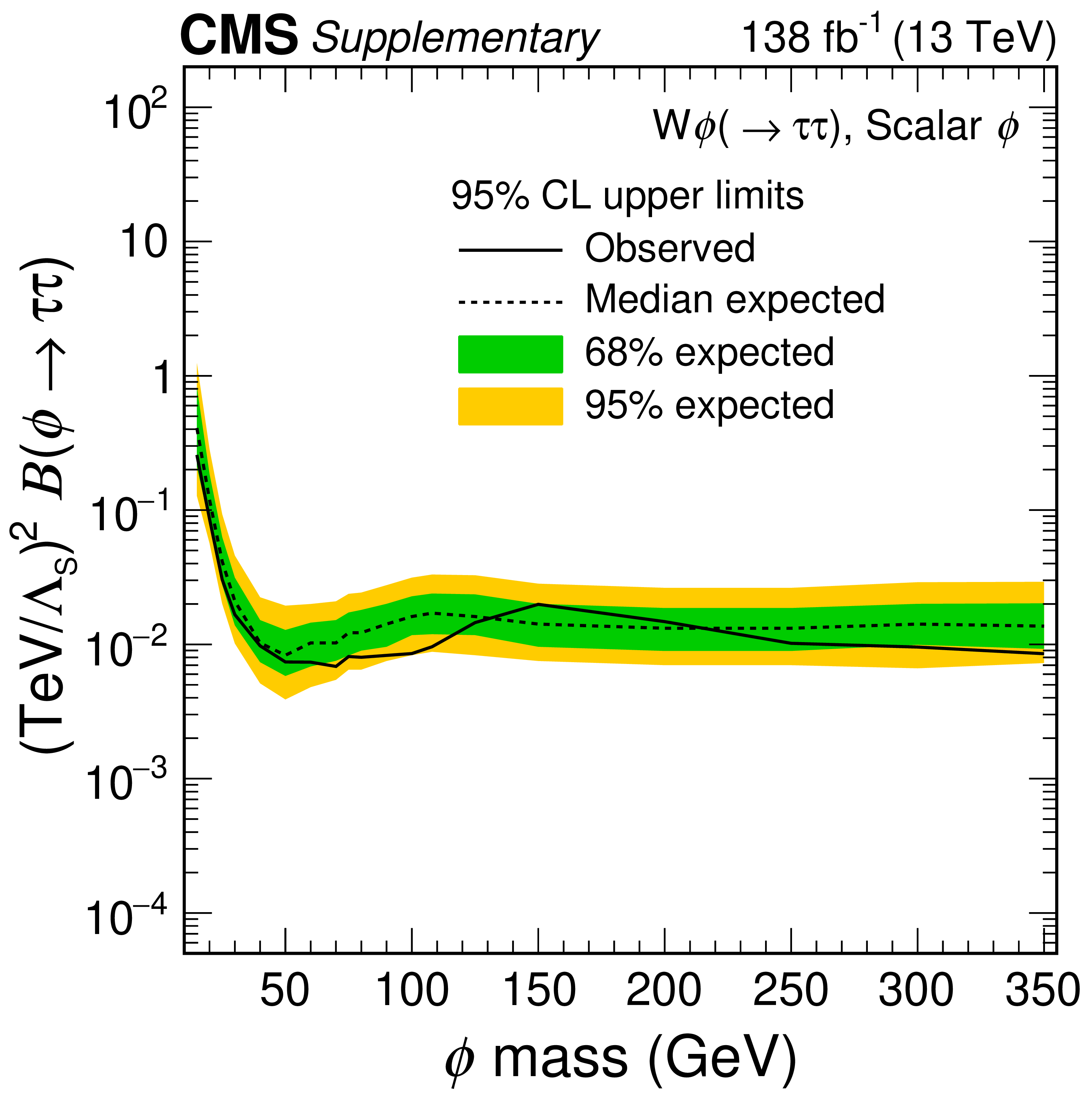
png pdf	Additional Figure 12: The 95% confidence level expected and observed upper limits on the product of $ (1/\Lambda_{\mathrm{S}})^2 $ and $ \mathcal{B}(\phi \to \tau\tau) $ of the $ {\mathrm{W}}{\phi} $ signal with scalar couplings, where $ \Lambda_{\mathrm{S}} $ denotes the mass scale of the effective interaction and $ \mathcal{B}(\phi \to \tau\tau) $ is the branching fraction of the $ \phi $ boson into a tau pair.
png pdf	Additional Figure 13: The 95% confidence level expected and observed upper limits on the product of $ (1/\Lambda_{\mathrm{PS}})^2 $ and $ \mathcal{B}(\phi \to \mathrm{e}\mathrm{e}) $ of the $ {\mathrm{W}}{\phi} $ signal with pseudoscalar couplings, where $ \Lambda_{\mathrm{PS}} $ denotes the mass scale of the effective interaction and $ \mathcal{B}(\phi \to \mathrm{e}\mathrm{e}) $ is the branching fraction of the $ \phi $ boson into an electron pair. The vertical gray band indicates the mass region not considered in the analysis.
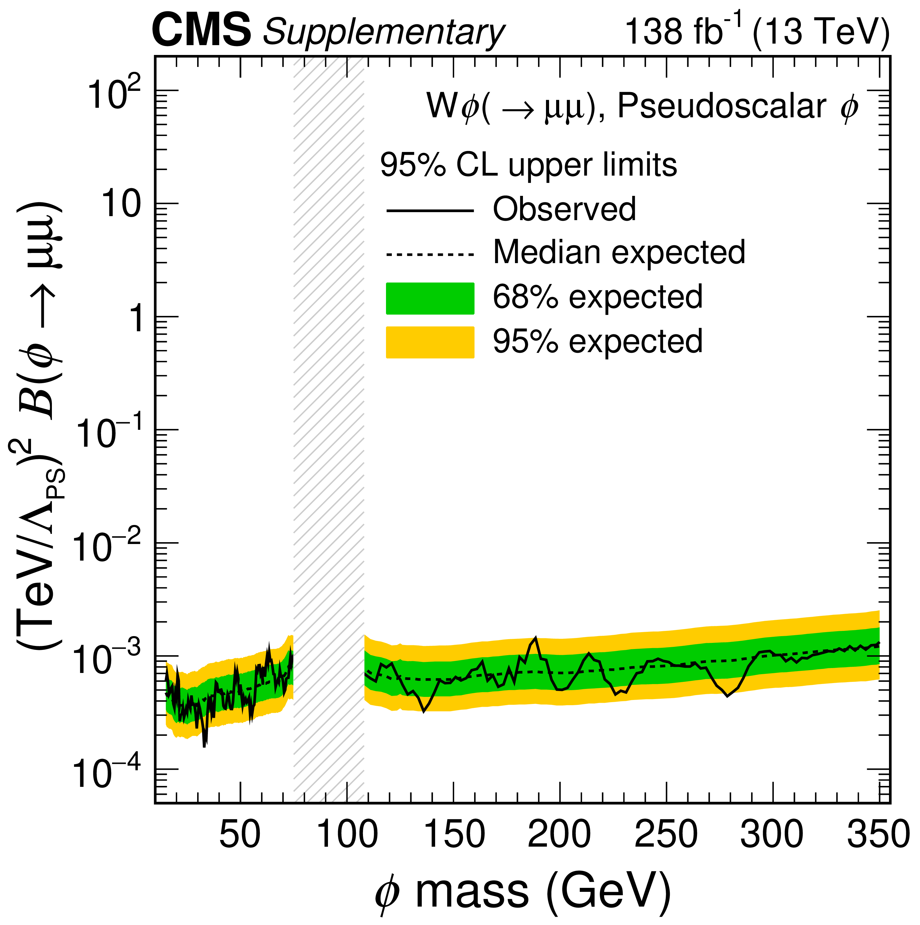
png pdf	Additional Figure 14: The 95% confidence level expected and observed upper limits on the product of $ (1/\Lambda_{\mathrm{PS}})^2 $ and $ \mathcal{B}(\phi \to \mu\mu) $ of the $ {\mathrm{W}}{\phi} $ signal with pseudoscalar couplings, where $ \Lambda_{\mathrm{PS}} $ denotes the mass scale of the effective interaction and $ \mathcal{B}(\phi \to \mu\mu) $ is the branching fraction of the $ \phi $ boson into a muon pair. The vertical gray band indicates the mass region not considered in the analysis.
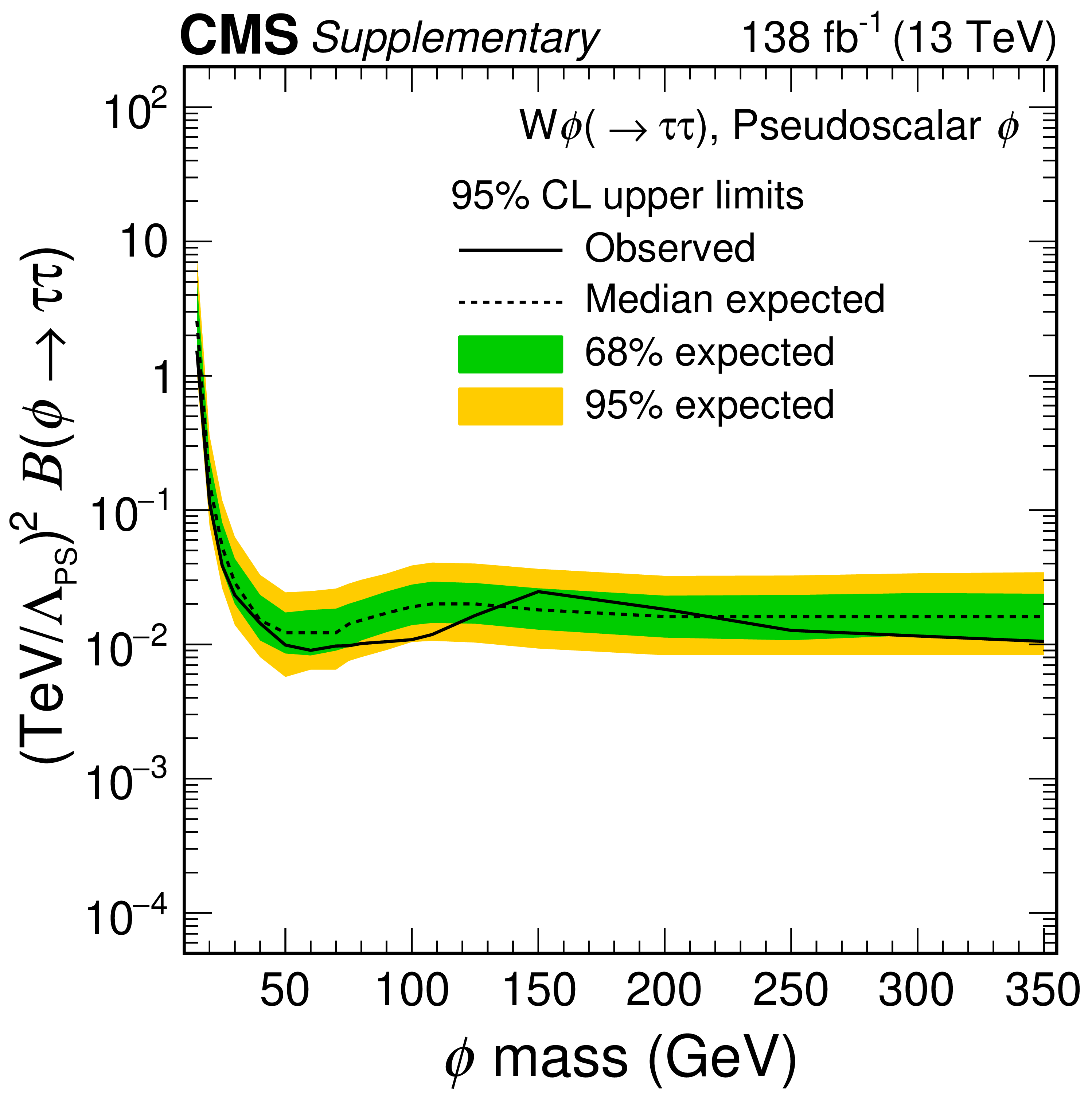
png pdf	Additional Figure 15: The 95% confidence level expected and observed upper limits on the product of $ (1/\Lambda_{\mathrm{PS}})^2 $ and $ \mathcal{B}(\phi \to \tau\tau) $ of the $ {\mathrm{W}}{\phi} $ signal with pseudoscalar couplings, where $ \Lambda_{\mathrm{PS}} $ denotes the mass scale of the effective interaction and $ \mathcal{B}(\phi \to \tau\tau) $ is the branching fraction of the $ \phi $ boson into a tau pair.
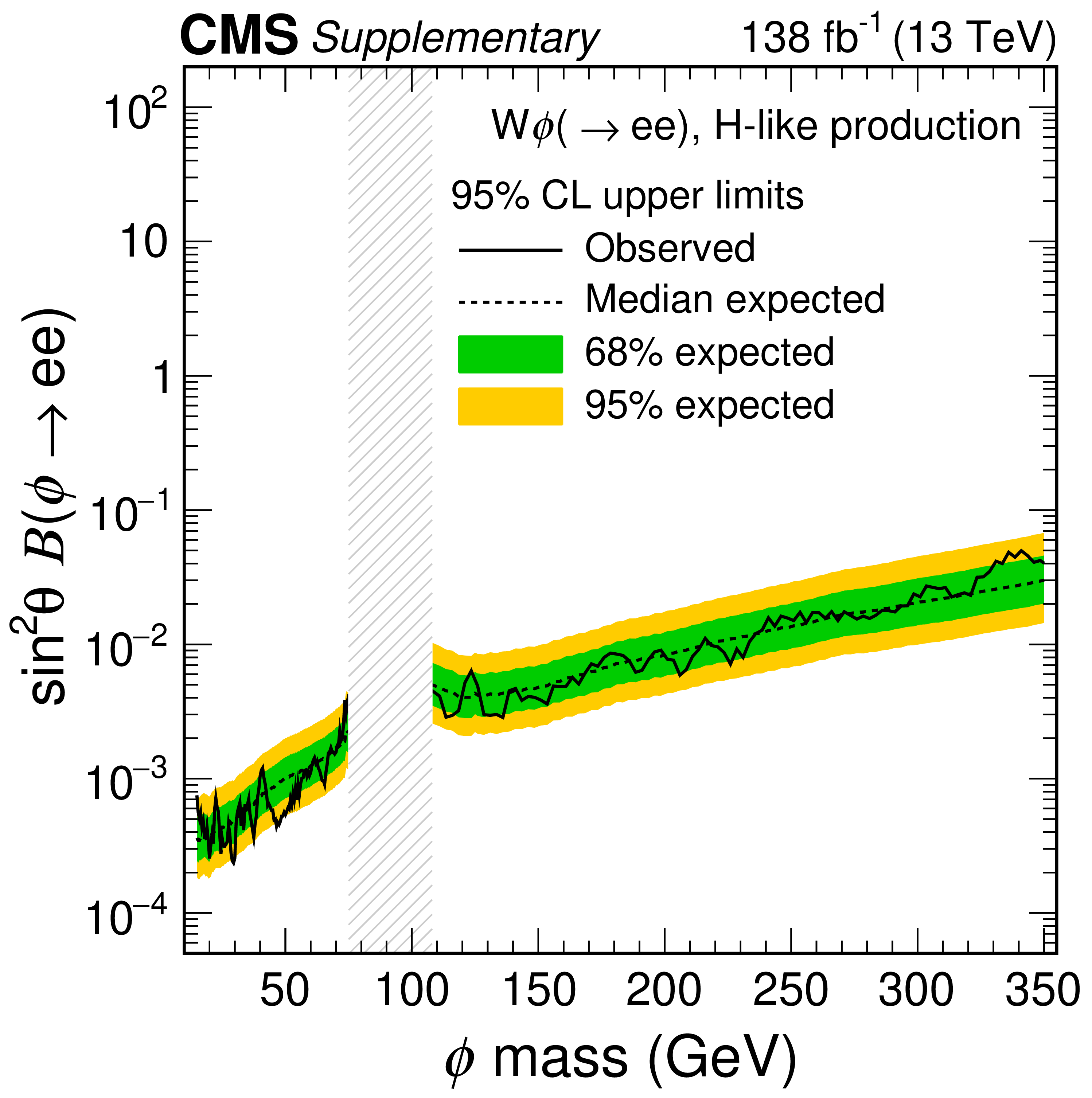
png pdf	Additional Figure 16: The 95% confidence level expected and observed upper limits on the product of $ \sin^2\theta $ and $ \mathcal{B}(\phi \to \mathrm{e}\mathrm{e}) $ of the $ {\mathrm{W}}{\phi} $ signal with H-like production, where $ \theta $ denotes the mixing angle of the Higgs boson with the $ \phi $ boson and $ \mathcal{B}(\phi \to \mathrm{e}\mathrm{e}) $ is the branching fraction of the $ \phi $ boson into an electron pair. The vertical gray band indicates the mass region not considered in the analysis.
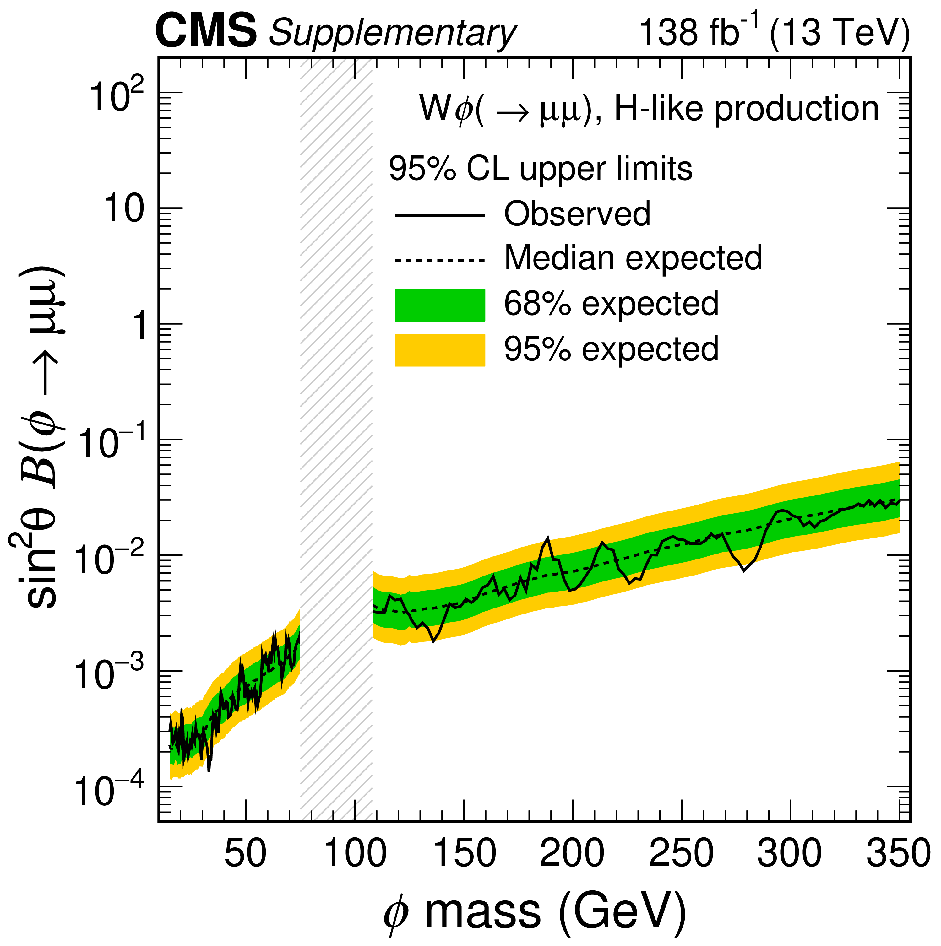
png pdf	Additional Figure 17: The 95% confidence level expected and observed upper limits on the product of $ \sin^2\theta $ and $ \mathcal{B}(\phi \to \mu\mu) $ of the $ {\mathrm{W}}{\phi} $ signal with H-like production, where $ \theta $ denotes the mixing angle of the Higgs boson with the $ \phi $ boson, and $ \mathcal{B}(\phi \to \mu\mu) $ is the branching fraction of the $ \phi $ boson into a muon pair. The vertical gray band indicates the mass region not considered in the analysis.
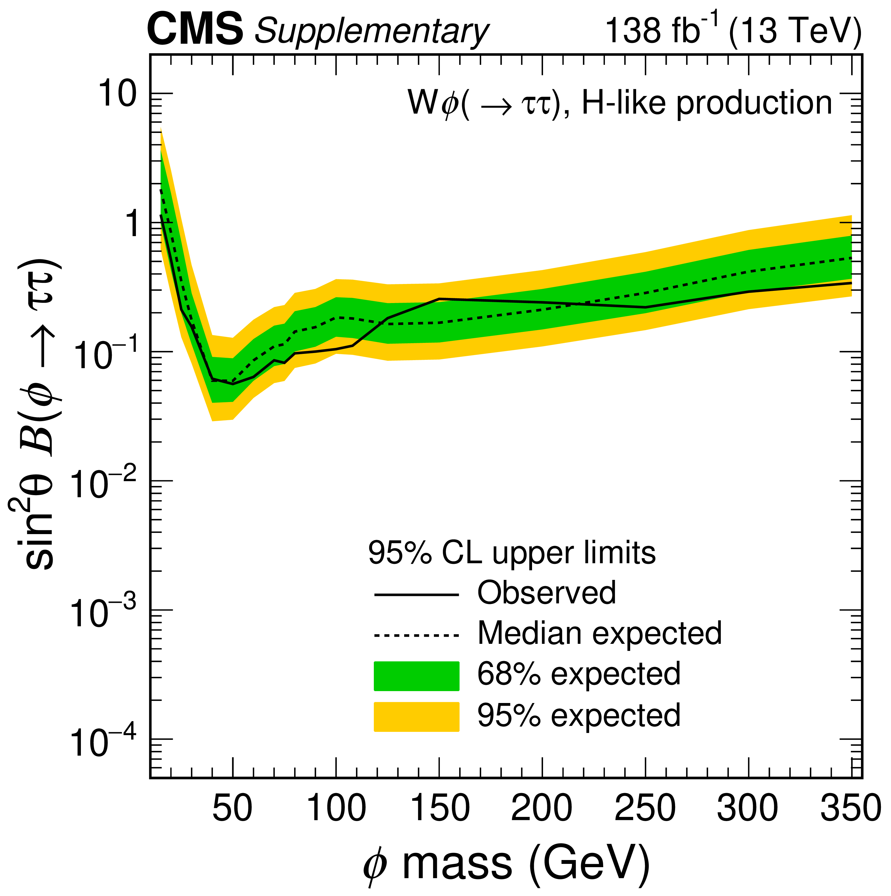
png pdf	Additional Figure 18: The 95% confidence level expected and observed upper limits on the product of $ \sin^2\theta $ and $ \mathcal{B}(\phi \to \tau\tau) $ of the $ {\mathrm{W}}{\phi} $ signal with H-like production, where $ \theta $ denotes the mixing angle of the Higgs boson with the $ \phi $ boson and $ \mathcal{B}(\phi \to \tau\tau) $ is the branching fraction of the $ \phi $ boson into a tau pair.
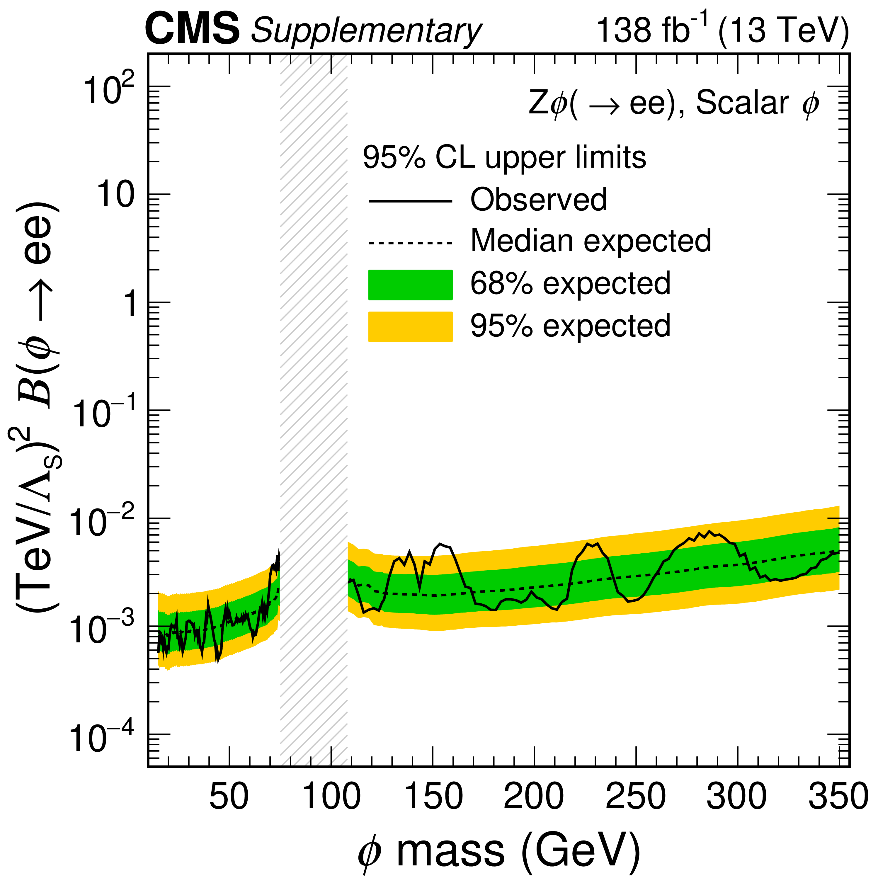
png pdf	Additional Figure 19: The 95% confidence level expected and observed upper limits on the product of $ (1/\Lambda_{\mathrm{S}})^2 $ and $ \mathcal{B}(\phi \to \mathrm{e}\mathrm{e}) $ of the $ {\mathrm{Z}}{\phi} $ signal with scalar couplings, where $ \Lambda_{\mathrm{S}} $ denotes the mass scale of the effective interaction and $ \mathcal{B}(\phi \to \mathrm{e}\mathrm{e}) $ is the branching fraction of the $ \phi $ boson into an electron pair. The vertical gray band indicates the mass region not considered in the analysis.
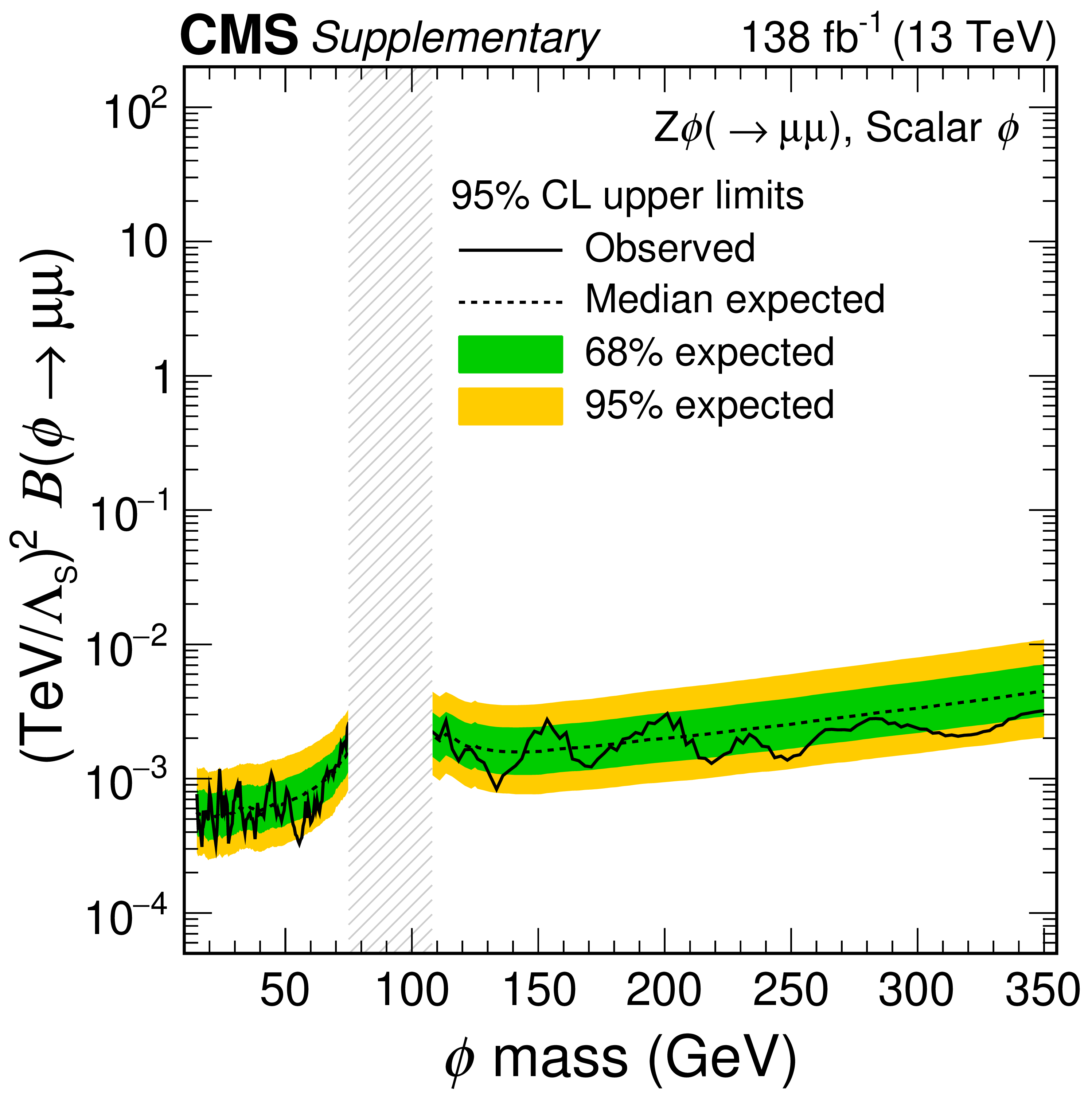
png pdf	Additional Figure 20: The 95% confidence level expected and observed upper limits on the product of $ (1/\Lambda_{\mathrm{S}})^2 $ and $ \mathcal{B}(\phi \to \mu\mu) $ of the $ {\mathrm{Z}}{\phi} $ signal with scalar couplings, where $ \Lambda_{\mathrm{S}} $ denotes the mass scale of the effective interaction and $ \mathcal{B}(\phi \to \mu\mu) $ is the branching fraction of the $ \phi $ boson into a muon pair. The vertical gray band indicates the mass region not considered in the analysis.
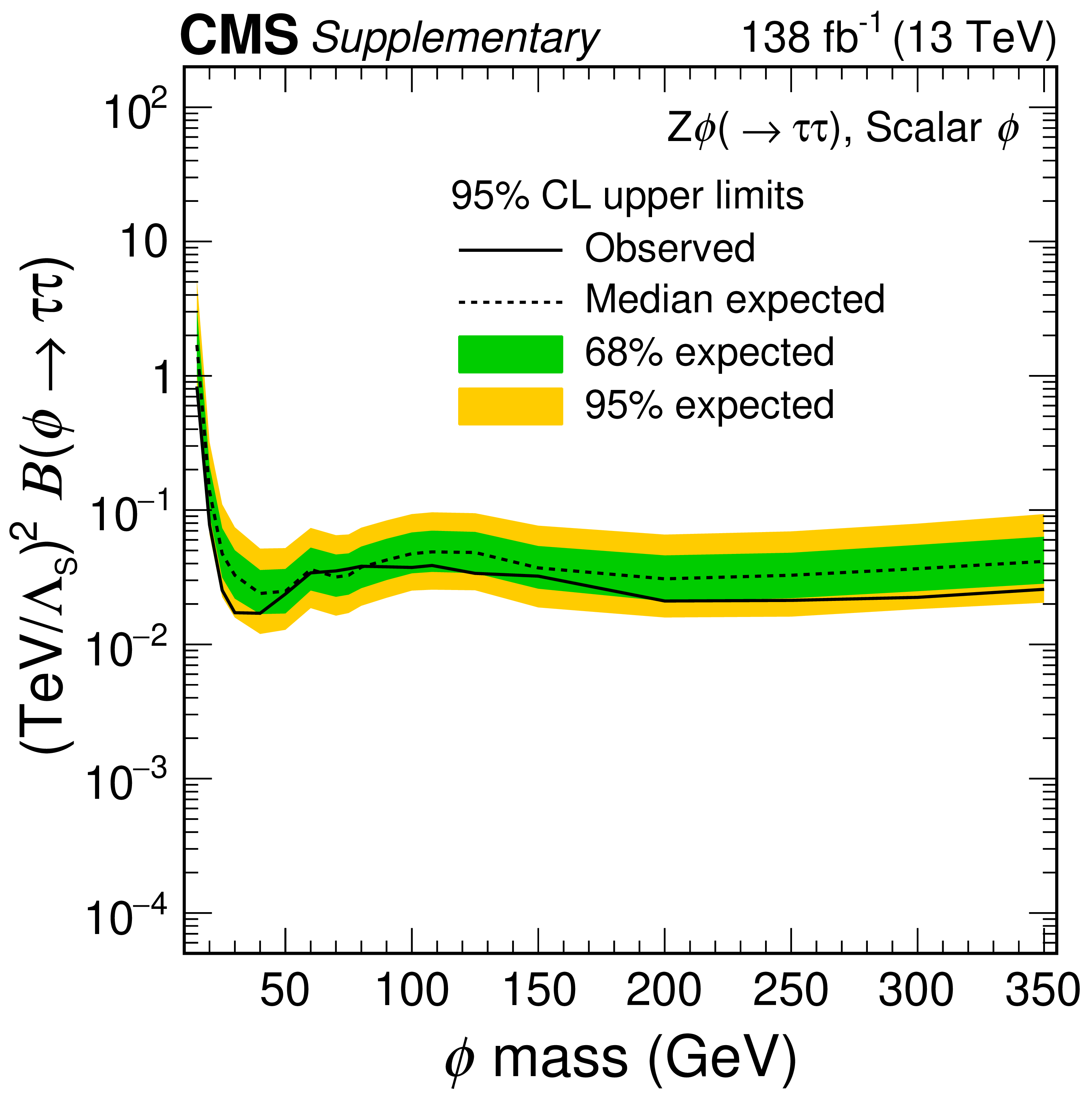
png pdf	Additional Figure 21: The 95% confidence level expected and observed upper limits on the product of $ (1/\Lambda_{\mathrm{S}})^2 $ and $ \mathcal{B}(\phi \to \tau\tau) $ of the $ {\mathrm{Z}}{\phi} $ signal with scalar couplings, where $ \Lambda_{\mathrm{S}} $ denotes the mass scale of the effective interaction and $ \mathcal{B}(\phi \to \tau\tau) $ is the branching fraction of the $ \phi $ boson into a tau pair.
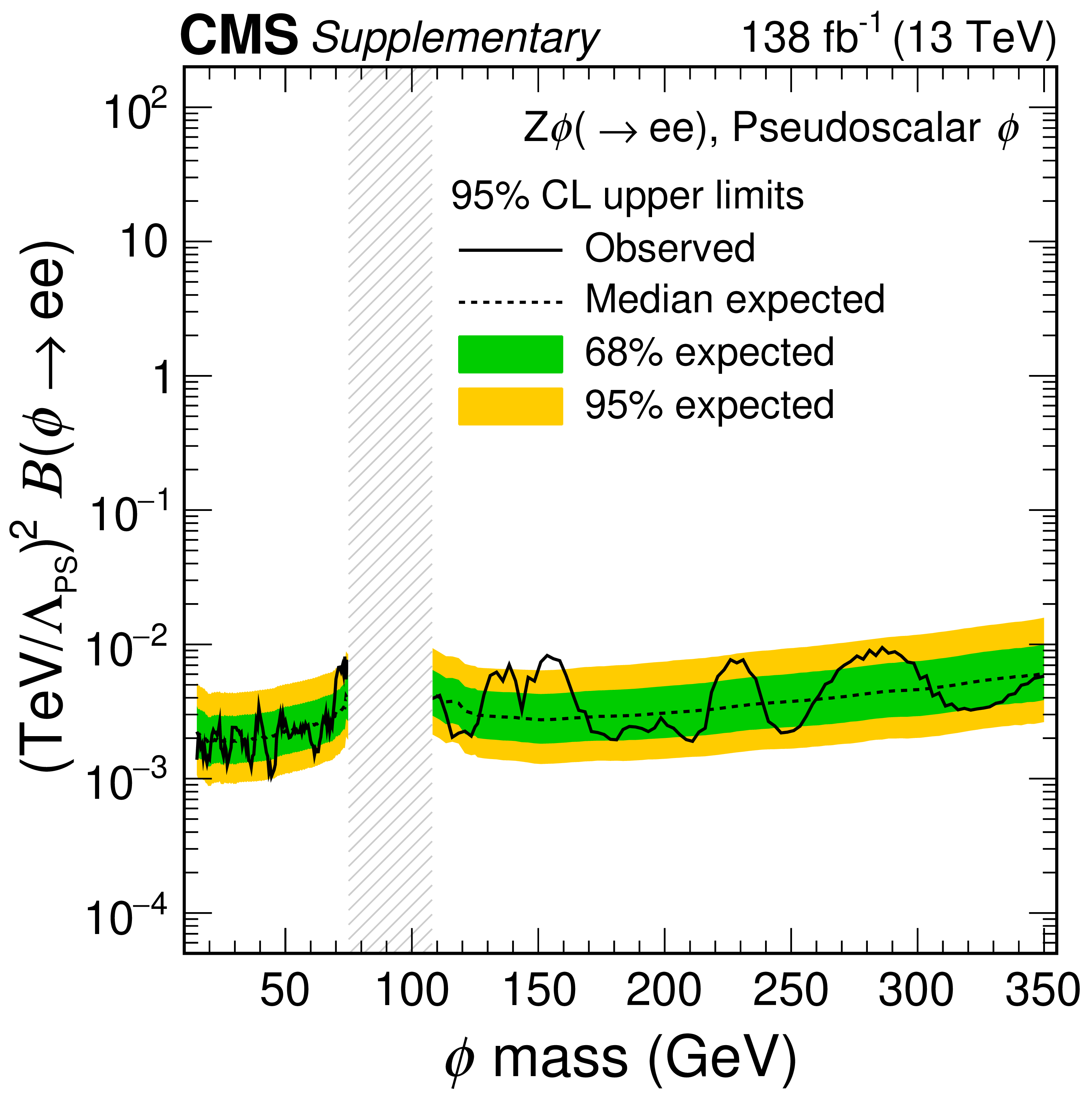
png pdf	Additional Figure 22: The 95% confidence level expected and observed upper limits on the product of $ (1/\Lambda_{\mathrm{PS}})^2 $ and $ \mathcal{B}(\phi \to \mathrm{e}\mathrm{e}) $ of the $ {\mathrm{Z}}{\phi} $ signal with pseudoscalar couplings, where $ \Lambda_{\mathrm{S}} $ denotes the mass scale of the effective interaction and $ \mathcal{B}(\phi \to \mathrm{e}\mathrm{e}) $ is the branching fraction of the $ \phi $ boson into an electron pair. The vertical gray band indicates the mass region not considered in the analysis.
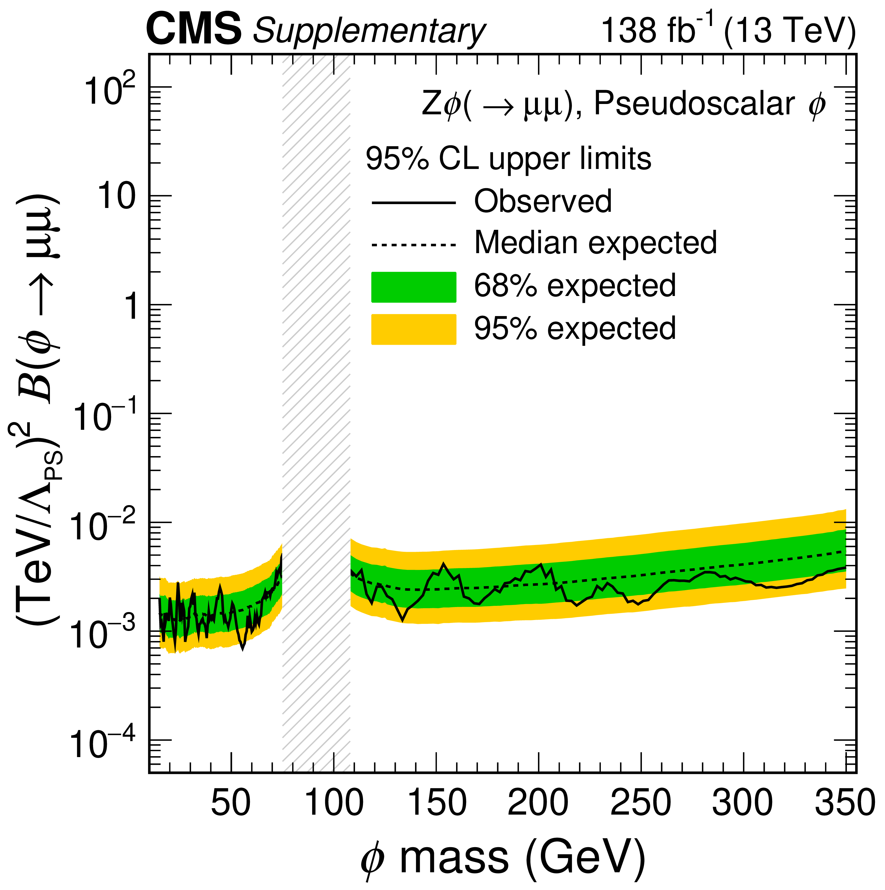
png pdf	Additional Figure 23: The 95% confidence level expected and observed upper limits on the product of $ (1/\Lambda_{\mathrm{PS}})^2 $ and $ \mathcal{B}(\phi \to \mu\mu) $ of the $ {\mathrm{Z}}{\phi} $ signal with pseudoscalar couplings, where $ \Lambda_{\mathrm{PS}} $ denotes the mass scale of the effective interaction and $ \mathcal{B}(\phi \to \mu\mu) $ is the branching fraction of the $ \phi $ boson into a muon pair. The vertical gray band indicates the mass region not considered in the analysis.
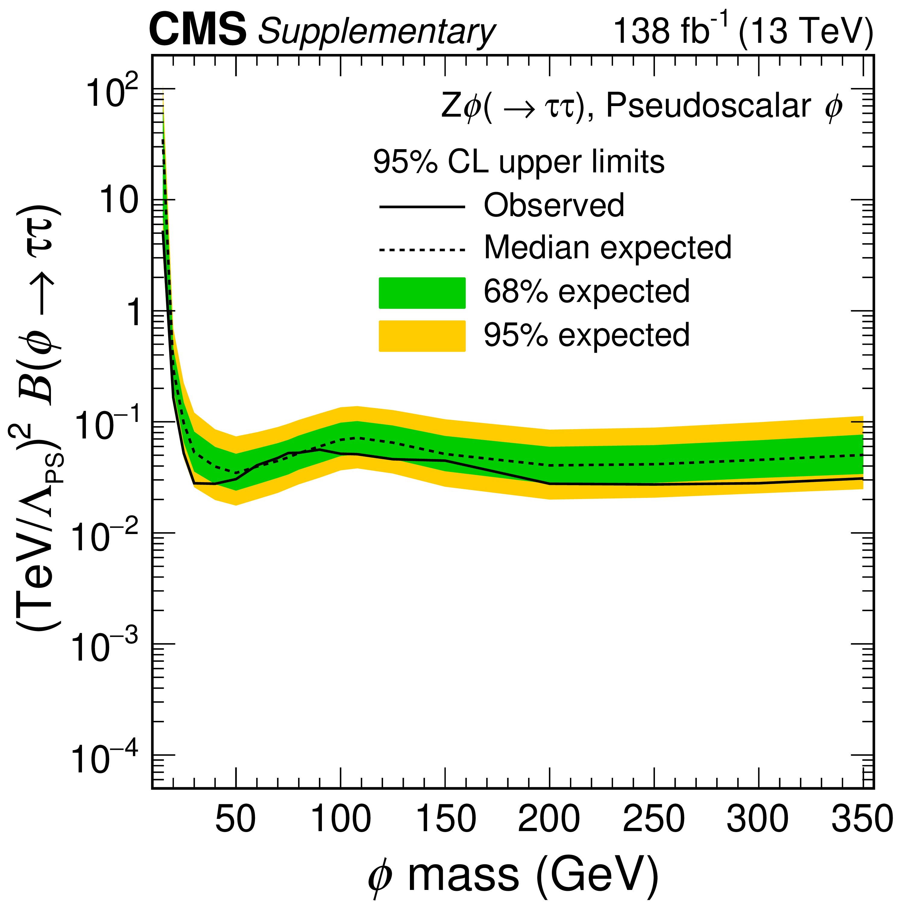
png pdf	Additional Figure 24: The 95% confidence level expected and observed upper limits on the product of $ (1/\Lambda_{\mathrm{PS}})^2 $ and $ \mathcal{B}(\phi \to \tau\tau) $ of the $ {\mathrm{Z}}{\phi} $ signal with pseudoscalar couplings, where $ \Lambda_{\mathrm{PS}} $ denotes the mass scale of the effective interaction and $ \mathcal{B}(\phi \to \tau\tau) $ is the branching fraction of the $ \phi $ boson into a tau pair.
png pdf	Additional Figure 25: The 95% confidence level expected and observed upper limits on the product of $ \sin^2\theta $ and $ \mathcal{B}(\phi \to \mathrm{e}\mathrm{e}) $ of the $ {\mathrm{Z}}{\phi} $ signal with H-like production, where $ \theta $ denotes the mixing angle of the Higgs boson with the $ \phi $ boson and $ \mathcal{B}(\phi \to \mathrm{e}\mathrm{e}) $ is the branching fraction of the $ \phi $ boson into an electron pair. The vertical gray band indicates the mass region not considered in the analysis.
png pdf	Additional Figure 26: The 95% confidence level expected and observed upper limits on the product of $ \sin^2\theta $ and $ \mathcal{B}(\phi \to \mu\mu) $ of the $ {\mathrm{Z}}{\phi} $ signal with H-like production, where $ \theta $ denotes the mixing angle of the Higgs boson with the $ \phi $ boson and $ \mathcal{B}(\phi \to \mu\mu) $ is the branching fraction of the $ \phi $ boson into a muon pair. The vertical gray band indicates the mass region not considered in the analysis.
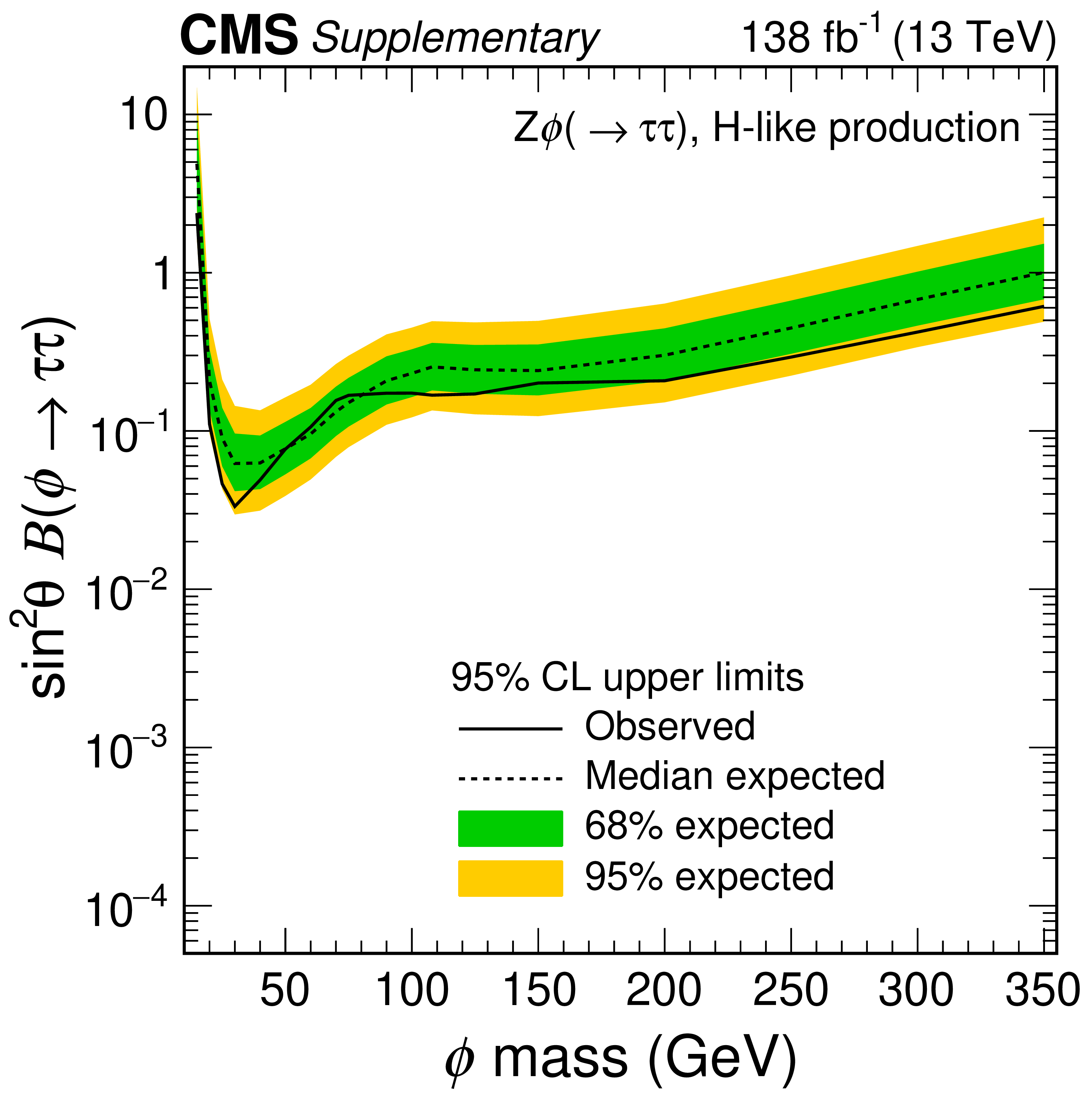
png pdf	Additional Figure 27: The 95% confidence level expected and observed upper limits on the product of $ \sin^2\theta $ and $ \mathcal{B}(\phi \to \tau\tau) $ of the $ {\mathrm{Z}}{\phi} $ signal with H-like production, where $ \theta $ denotes the mixing angle of the Higgs boson with the $ \phi $ boson and $ \mathcal{B}(\phi \to \tau\tau) $ is the branching fraction of the $ \phi $ boson into a tau pair.
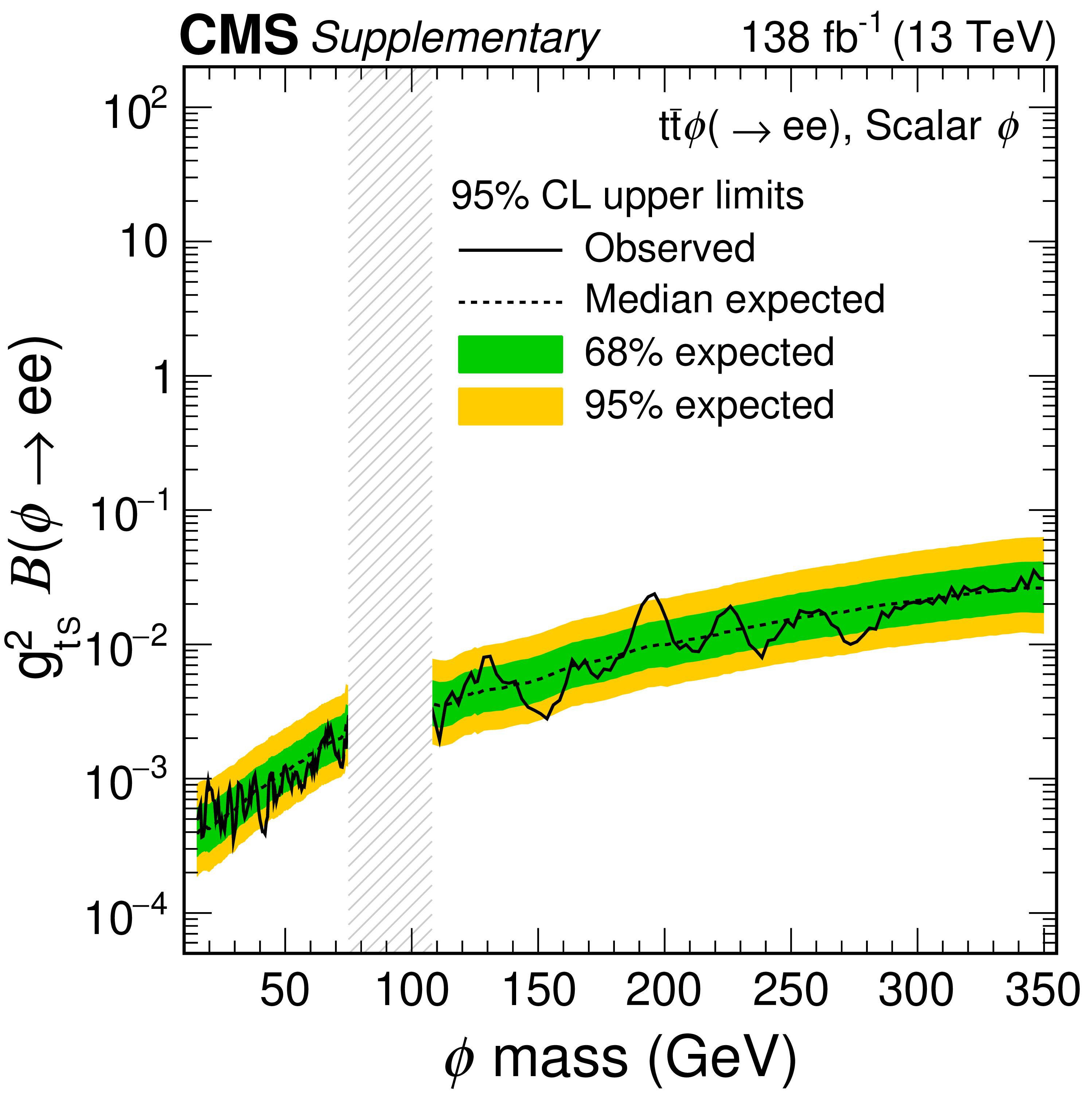
png pdf	Additional Figure 28: The 95% confidence level expected and observed upper limits on the product of $ {\mathrm{g}}_{{\mathrm{t S}}}^2 $ and $ \mathcal{B}(\phi \to \mathrm{e}\mathrm{e}) $ of the $ {{\mathrm{t}\overline{\mathrm{t}}} }{\phi} $ signal with scalar couplings, where $ {\mathrm{g}}_{{\mathrm{t S}}} $ denotes the coupling of the $ \phi $ boson to the top quark and $ \mathcal{B}(\phi \to \mathrm{e}\mathrm{e}) $ is the branching fraction of the $ \phi $ boson into an electron pair. The vertical gray band indicates the mass region not considered in the analysis.
png pdf	Additional Figure 29: The 95% confidence level expected and observed upper limits on the product of $ {\mathrm{g}}_{{\mathrm{t S}}}^2 $ and $ \mathcal{B}(\phi \to \mu\mu) $ of the $ {{\mathrm{t}\overline{\mathrm{t}}} }{\phi} $ signal with scalar couplings, where $ {\mathrm{g}}_{{\mathrm{t S}}} $ denotes the coupling of the $ \phi $ boson to the top quark and $ \mathcal{B}(\phi \to \mu\mu) $ is the branching fraction of the $ \phi $ boson into a muon pair. The vertical gray band indicates the mass region not considered in the analysis.
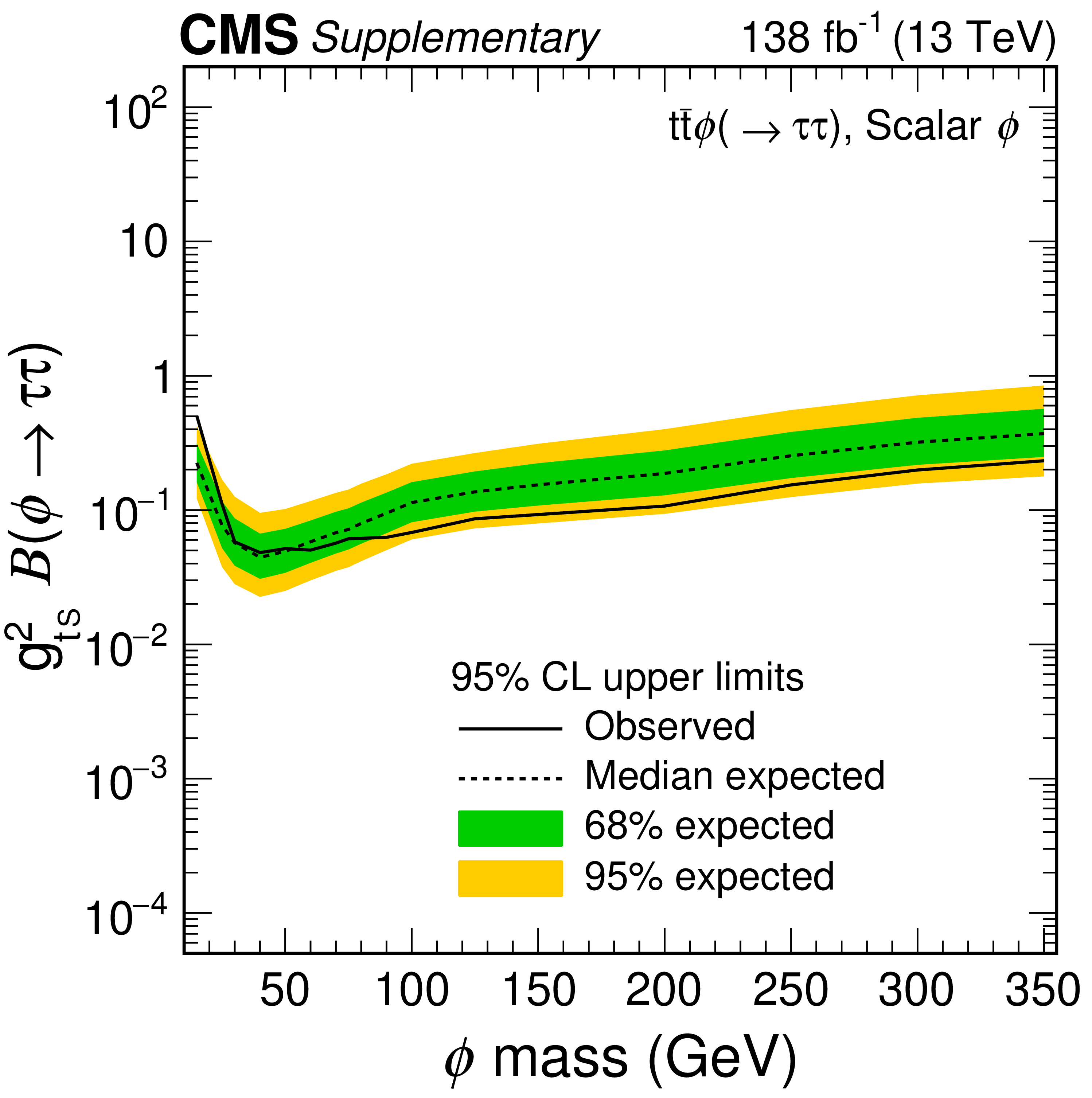
png pdf	Additional Figure 30: The 95% confidence level expected and observed upper limits on the product of $ {\mathrm{g}}_{{\mathrm{t S}}}^2 $ and $ \mathcal{B}(\phi \to \tau\tau) $ of the $ {{\mathrm{t}\overline{\mathrm{t}}} }{\phi} $ signal with scalar couplings, where $ {\mathrm{g}}_{{\mathrm{t S}}} $ denotes the coupling of the $ \phi $ boson to the top quark and $ \mathcal{B}(\phi \to \tau\tau) $ is the branching fraction of the $ \phi $ boson into a ditau pair.
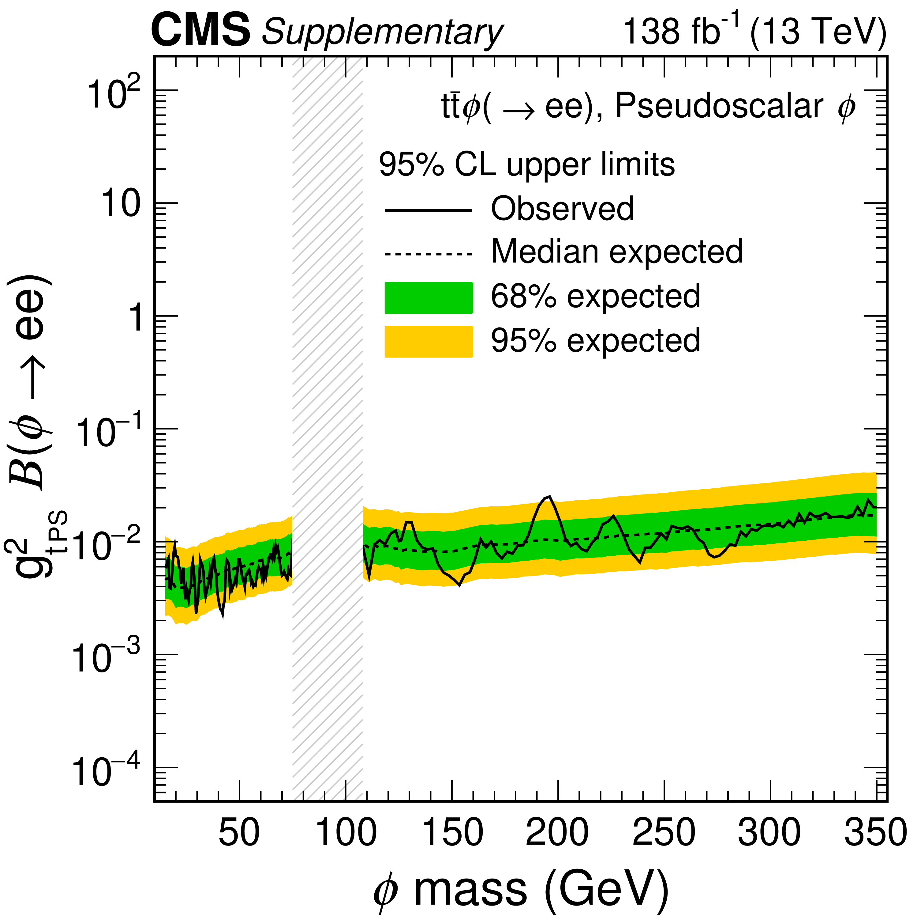
png pdf	Additional Figure 31: The 95% confidence level expected and observed upper limits on the product of $ {\mathrm{g}}_{{\mathrm{t PS}}}^2 $ and $ \mathcal{B}(\phi \to \mathrm{e}\mathrm{e}) $ of the $ {{\mathrm{t}\overline{\mathrm{t}}} }{\phi} $ signal with pseudoscalar couplings, where $ {\mathrm{g}}_{{\mathrm{t PS}}} $ denotes the coupling of the $ \phi $ boson to the top quark and $ \mathcal{B}(\phi \to \mathrm{e}\mathrm{e}) $ is the branching fraction of the $ \phi $ boson into an electron pair. The vertical gray band indicates the mass region not considered in the analysis.
png pdf	Additional Figure 32: The 95% confidence level expected and observed upper limits on the product of $ {\mathrm{g}}_{{\mathrm{t PS}}}^2 $ and $ \mathcal{B}(\phi \to \mu\mu) $ of the $ {{\mathrm{t}\overline{\mathrm{t}}} }{\phi} $ signal with pseudoscalar couplings, where $ {\mathrm{g}}_{{\mathrm{t PS}}} $ denotes the coupling of the $ \phi $ boson to the top quark and $ \mathcal{B}(\phi \to \mu\mu) $ is the branching fraction of the $ \phi $ boson into a muon pair. The vertical gray band indicates the mass region not considered in the analysis.
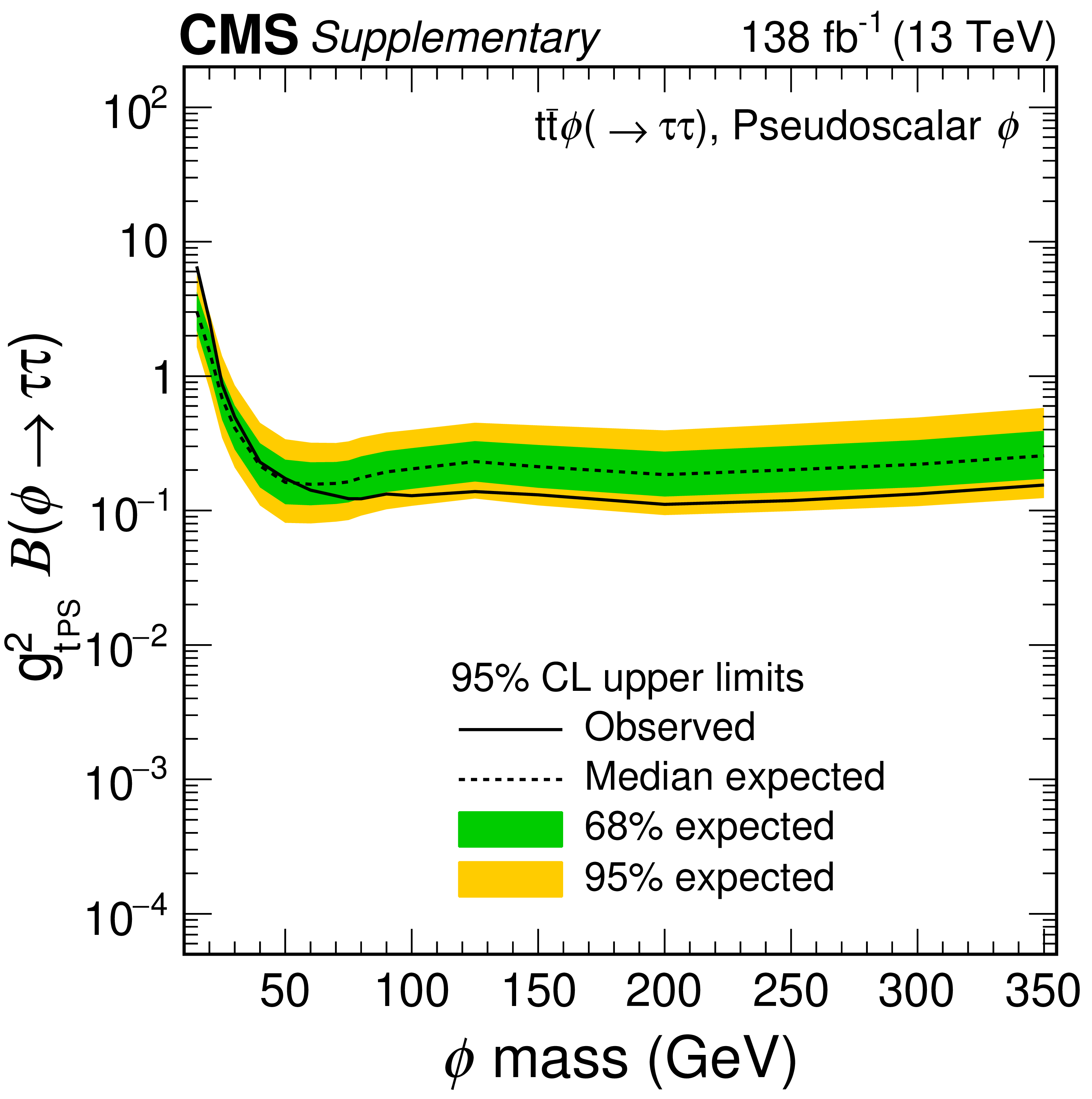
png pdf	Additional Figure 33: The 95% confidence level expected and observed upper limits on the product of $ {\mathrm{g}}_{{\mathrm{t PS}}}^2 $ and $ \mathcal{B}(\phi \to \tau\tau) $ of the $ {{\mathrm{t}\overline{\mathrm{t}}} }{\phi} $ signal with pseudoscalar couplings, where $ {\mathrm{g}}_{{\mathrm{t PS}}} $ denotes the coupling of the $ \phi $ boson to the top quark and $ \mathcal{B}(\phi \to \tau\tau) $ is the branching fraction of the $ \phi $ boson into a tau pair.
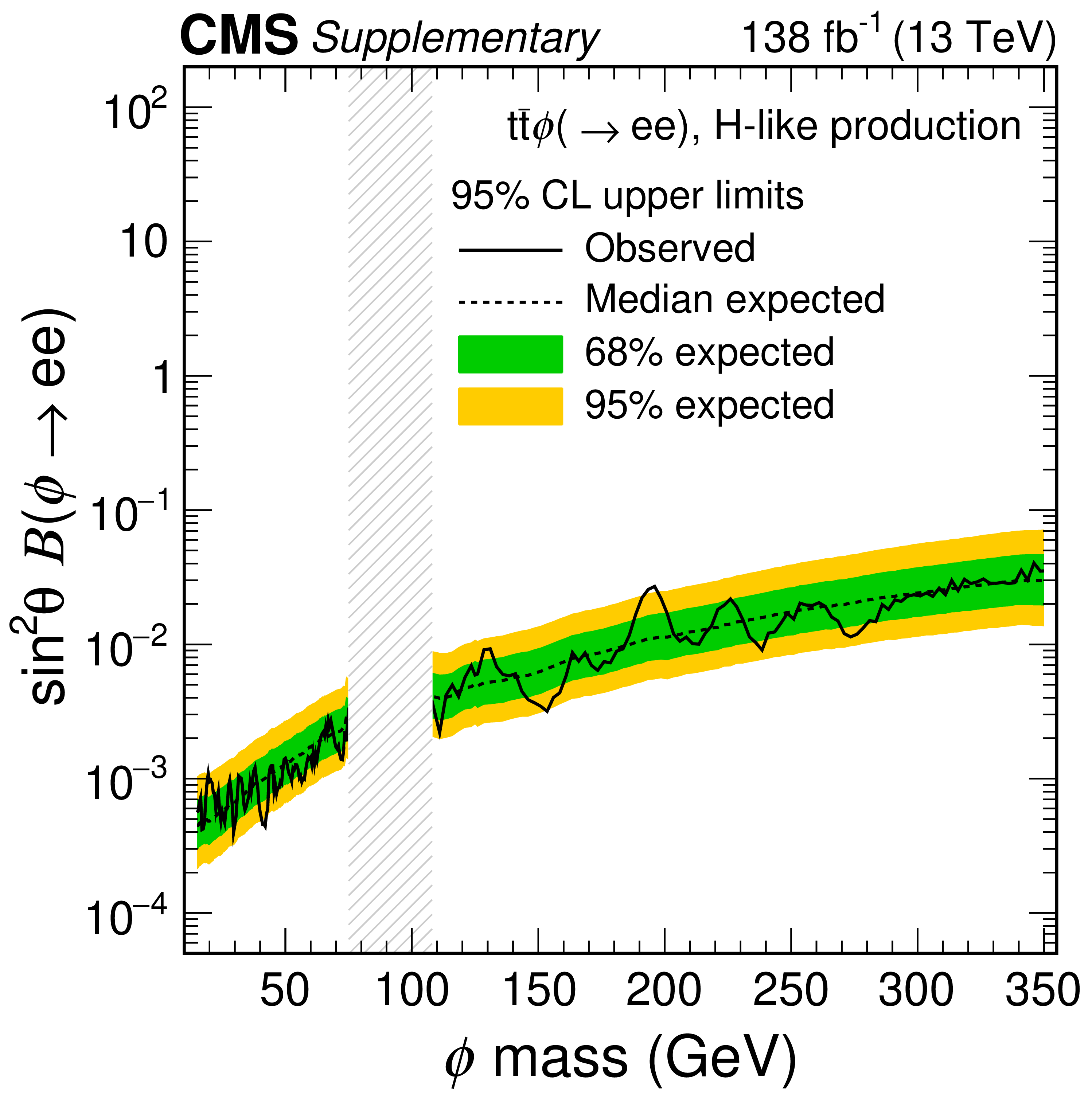
png pdf	Additional Figure 34: The 95% confidence level expected and observed upper limits on the product of $ \sin^2\theta $ and $ \mathcal{B}(\phi \to \mathrm{e}\mathrm{e}) $ of the $ {{\mathrm{t}\overline{\mathrm{t}}} }{\phi} $ signal with H-like production, where $ \theta $ denotes the mixing angle of the Higgs boson with the $ \phi $ boson and $ \mathcal{B}(\phi \to \mathrm{e}\mathrm{e}) $ is the branching fraction of the $ \phi $ boson into an electron pair. The vertical gray band indicates the mass region not considered in the analysis.
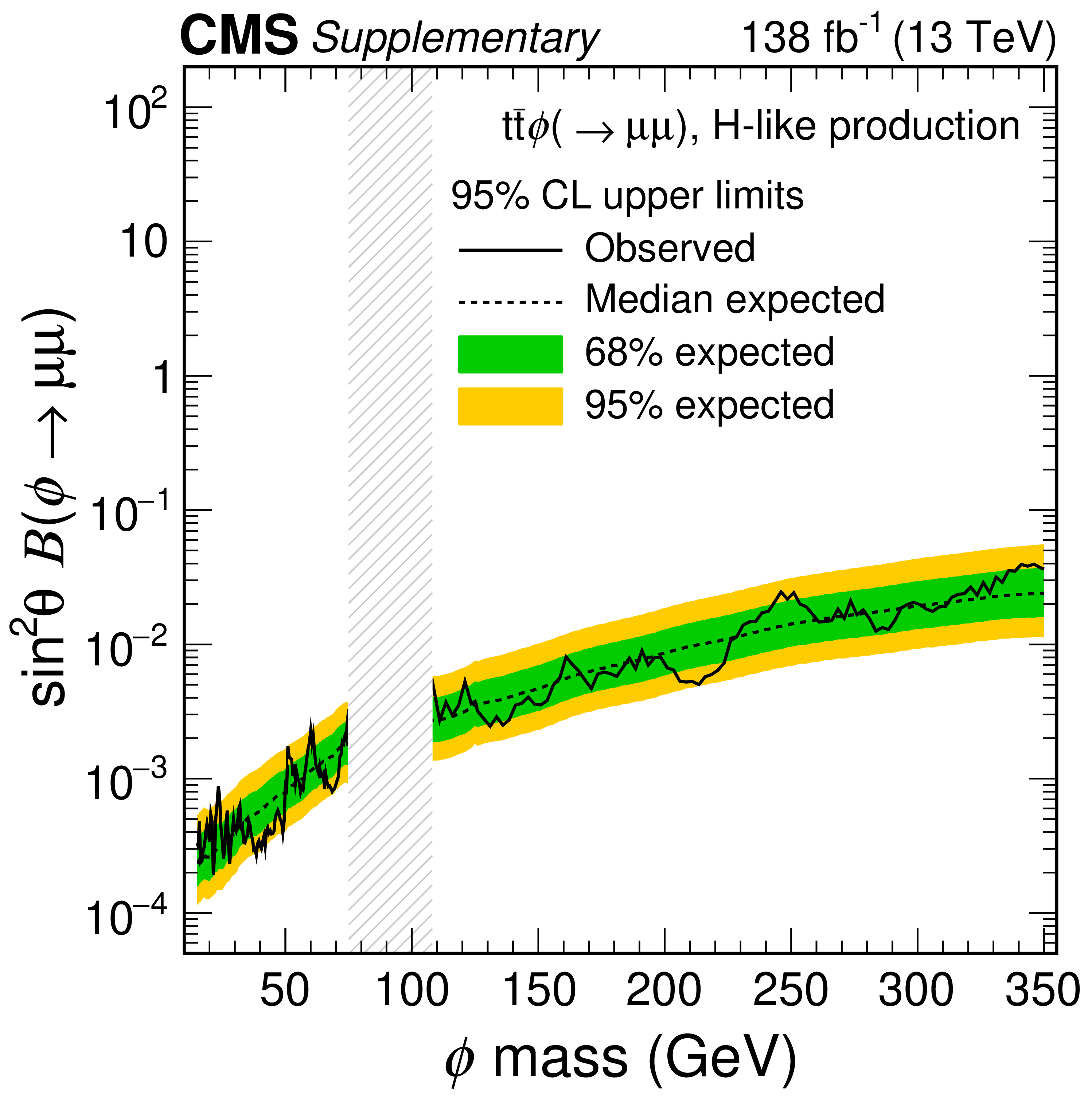
png pdf	Additional Figure 35: The 95% confidence level expected and observed upper limits on the product of $ \sin^2\theta $ and $ \mathcal{B}(\phi \to \mu\mu) $ of the $ {{\mathrm{t}\overline{\mathrm{t}}} }{\phi} $ signal with H-like production, where $ \theta $ denotes the mixing angle of the Higgs boson with the $ \phi $ boson and $ \mathcal{B}(\phi \to \mu\mu) $ is the branching fraction of the $ \phi $ boson into a muon pair. The vertical gray band indicates the mass region not considered in the analysis.
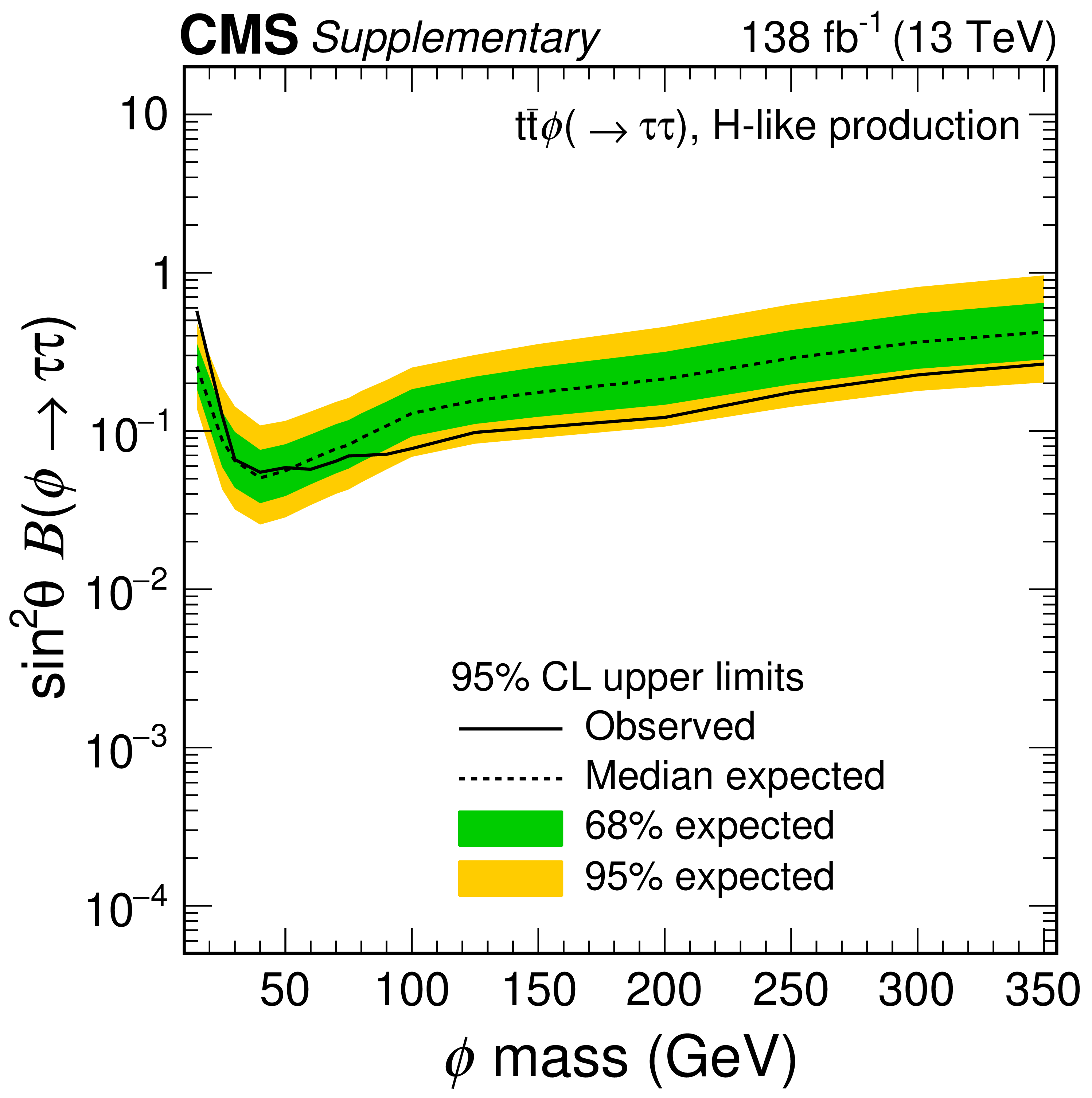
png pdf	Additional Figure 36: The 95% confidence level expected and observed upper limits on the product of $ \sin^2\theta $ and $ \mathcal{B}(\phi \to \tau\tau) $ of the $ {{\mathrm{t}\overline{\mathrm{t}}} }{\phi} $ signal with H-like production, where $ \theta $ denotes the mixing angle of the Higgs boson with the $ \phi $ boson and $ \mathcal{B}(\phi \to \tau\tau) $ is the branching fraction of the $ \phi $ boson into a tau pair.
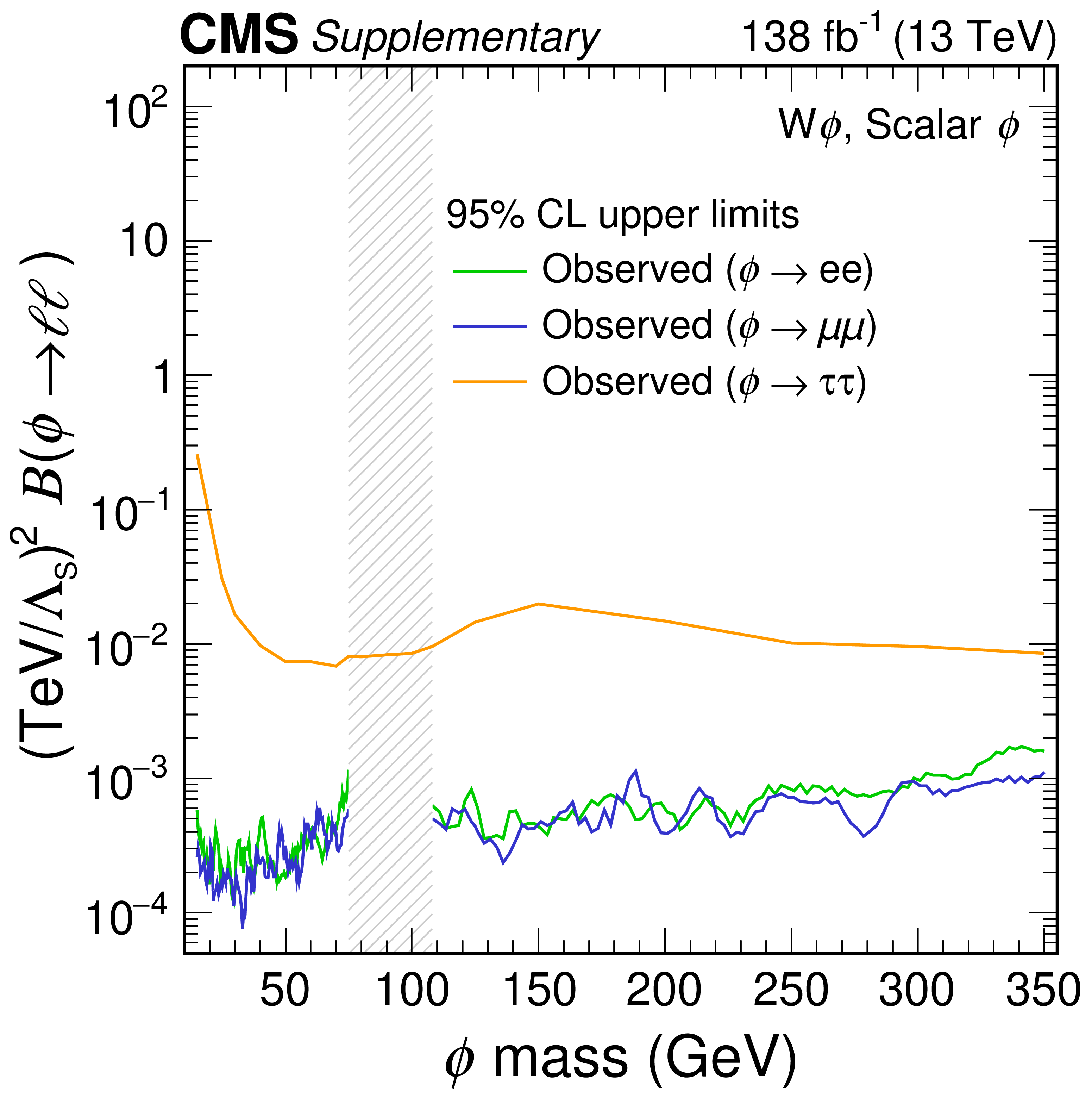
png pdf	Additional Figure 37: The 95% confidence level observed upper limits on the product of $ (1/\Lambda_{\mathrm{S}})^2 $ and $ \mathcal{B}(\phi \to \ell\ell) $ of the $ {\mathrm{W}}{\phi} $ signal with scalar couplings, where $ \Lambda_{\mathrm{S}} $ denotes the mass scale of the effective interaction and $ \mathcal{B}(\phi \to \ell\ell) $ is the branching fraction of the $ \phi $ boson into a lepton pair of given flavor. Exclusions on the dielectron, dimuon, and ditau decay scenarios of the $ \phi $ boson are shown with the green, blue, and orange solid lines. The vertical gray band indicates the mass region not considered in the analysis in the dielectron and dimuon decay scenarios of the $ \phi $ boson.
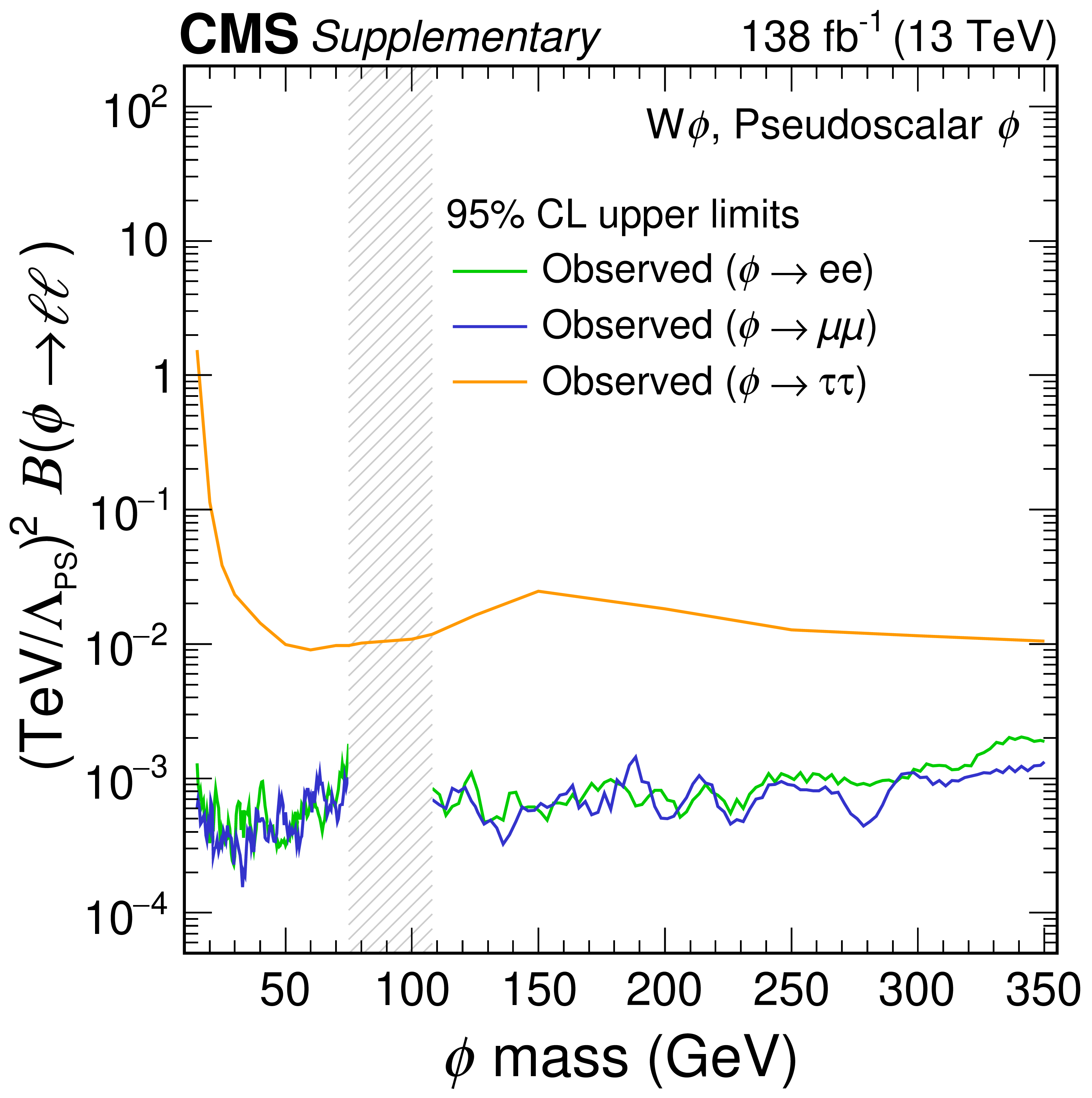
png pdf	Additional Figure 38: The 95% confidence level observed upper limits on the product of $ (1/\Lambda_{\mathrm{PS}})^2 $ and $ \mathcal{B}(\phi \to \ell\ell) $ of the $ {\mathrm{W}}{\phi} $ signal with pseudoscalar couplings, where $ \Lambda_{\mathrm{PS}} $ denotes the mass scale of the effective interaction and $ \mathcal{B}(\phi \to \ell\ell) $ is the branching fraction of the $ \phi $ boson into a lepton pair of given flavor. Exclusions on the dielectron, dimuon, and ditau decay scenarios of the $ \phi $ boson are shown with the green, blue, and orange solid lines. The vertical gray band indicates the mass region not considered in the analysis in the dielectron and dimuon decay scenarios of the $ \phi $ boson.
png pdf	Additional Figure 39: The 95% confidence level observed upper limits on the product of $ \sin^2\theta $ and $ \mathcal{B}(\phi \to \ell\ell) $ of the $ {\mathrm{W}}{\phi} $ signal with H-like production, where $ \theta $ denotes the mixing angle of the Higgs boson with the $ \phi $ boson and $ \mathcal{B}(\phi \to \ell\ell) $ is the branching fraction of the $ \phi $ boson into a lepton pair of given flavor. Exclusions on the dielectron, dimuon, and ditau decay scenarios of the $ \phi $ boson are shown with the green, blue, and orange solid lines, respectively. The vertical gray band indicates the mass region not considered in the analysis in the dielectron and dimuon decay scenarios of the $ \phi $ boson.
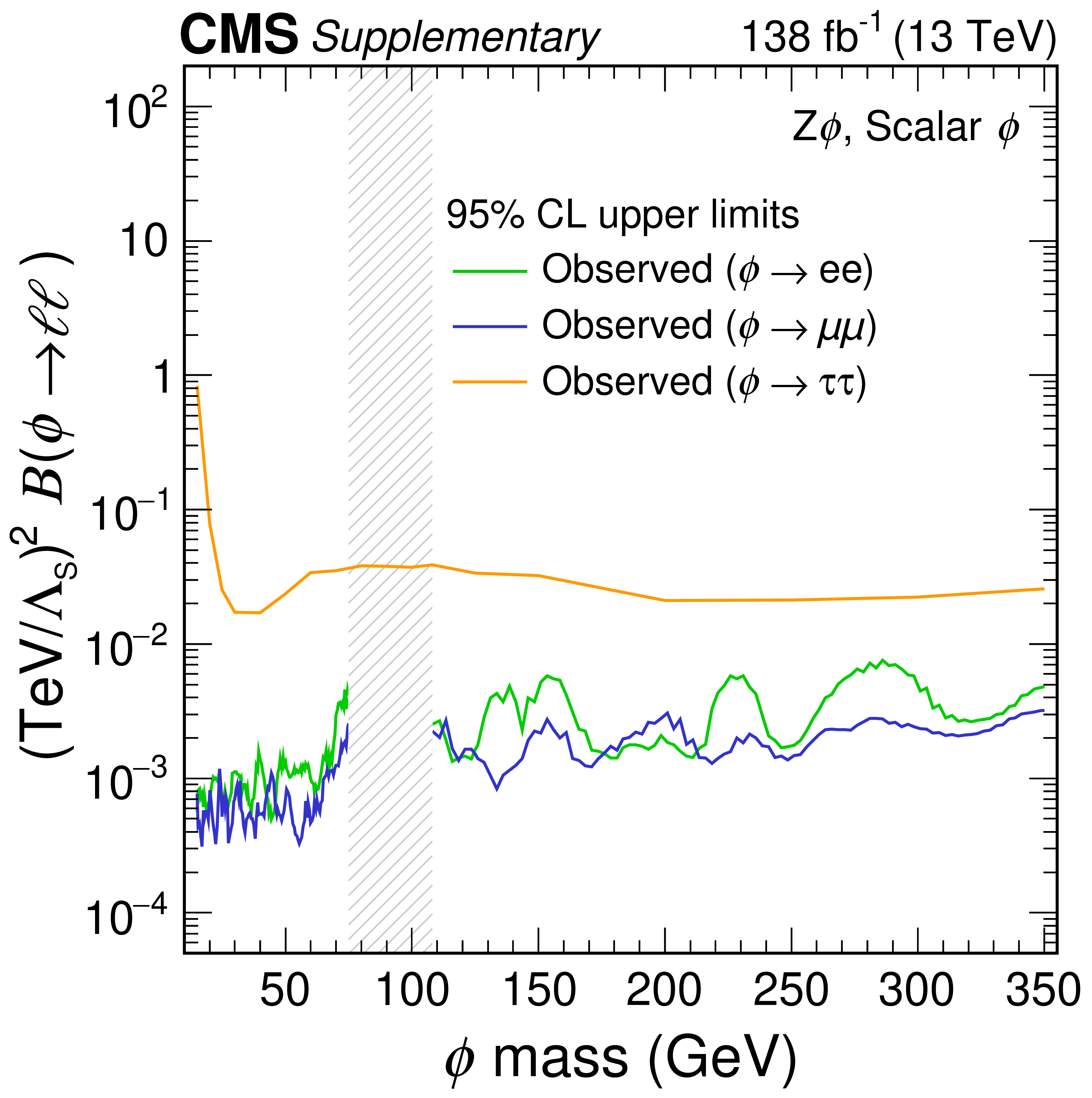
png pdf	Additional Figure 40: The 95% confidence level observed upper limits on the product of $ (1/\Lambda_{\mathrm{S}})^2 $ and $ \mathcal{B}(\phi \to \ell\ell) $ of the $ {\mathrm{Z}}{\phi} $ signal with scalar couplings, where $ \Lambda_{\mathrm{S}} $ denotes the mass scale of the effective interaction, and $ \mathcal{B}(\phi \to \ell\ell) $ is the branching fraction of the $ \phi $ boson into a lepton pair of given flavor. Exclusions on the dielectron, dimuon, and ditau decay scenarios of the $ \phi $ boson are shown with the green, blue, and orange solid lines, respectively. The vertical gray band indicates the mass region not considered in the analysis in the dielectron and dimuon decay scenarios of the $ \phi $ boson.
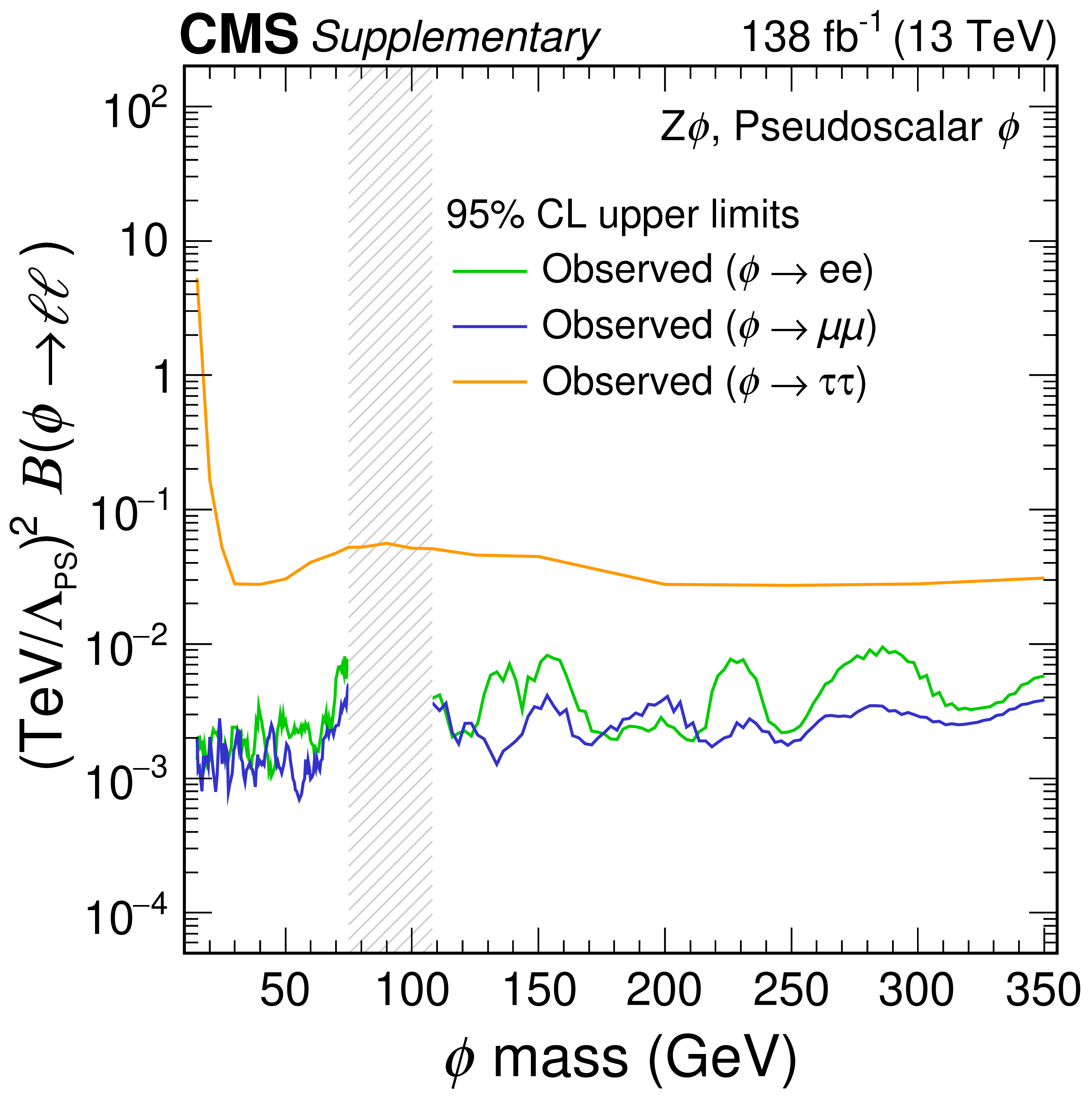
png pdf	Additional Figure 41: The 95% confidence level observed upper limits on the product of $ (1/\Lambda_{\mathrm{PS}})^2 $ and $ \mathcal{B}(\phi \to \ell\ell) $ of the $ {\mathrm{Z}}{\phi} $ signal with pseudoscalar couplings, where $ \Lambda_{\mathrm{PS}} $ denotes the mass scale of the effective interaction and $ \mathcal{B}(\phi \to \ell\ell) $ is the branching fraction of the $ \phi $ boson into a lepton pair of given flavor. Exclusions on the dielectron, dimuon, and ditau decay scenarios of the $ \phi $ boson are shown with the green, blue, and orange solid lines, respectively. The vertical gray band indicates the mass region not considered in the analysis in the dielectron and dimuon decay scenarios of the $ \phi $ boson.
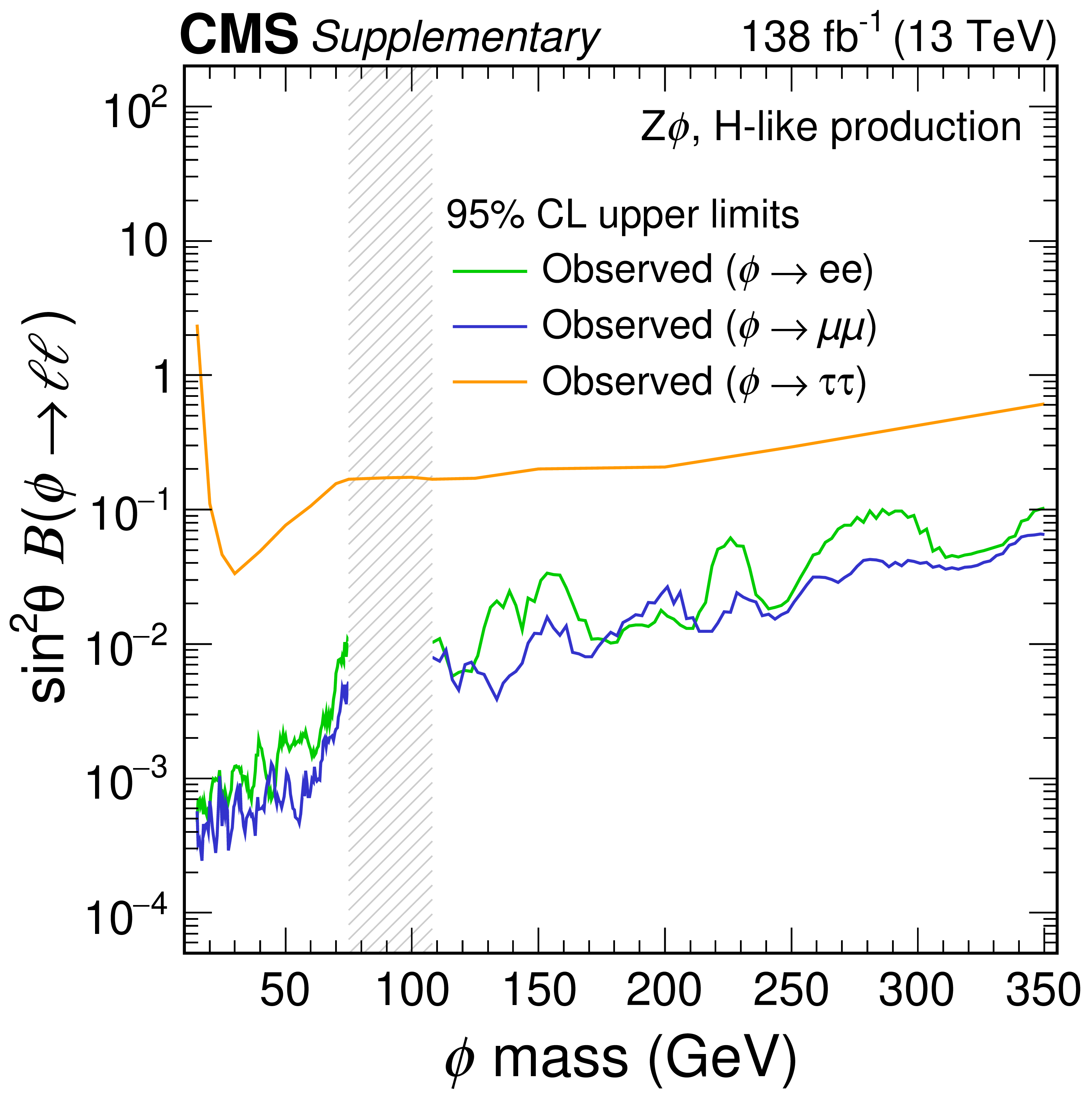
png pdf	Additional Figure 42: The 95% confidence level observed upper limits on the product of $ \sin^2\theta $ and $ \mathcal{B}(\phi \to \ell\ell) $ of the $ {\mathrm{Z}}{\phi} $ signal with H-like production, where $ \theta $ denotes the mixing angle of the Higgs boson with the $ \phi $ boson and $ \mathcal{B}(\phi \to \ell\ell) $ is the branching fraction of the $ \phi $ boson into a lepton pair of given flavor. Exclusions on the dielectron, dimuon, and ditau decay scenarios of the $ \phi $ boson are shown with the green, blue, and orange solid lines, respectively. The vertical gray band indicates the mass region not considered in the analysis in the dielectron and dimuon decay scenarios of the $ \phi $ boson.
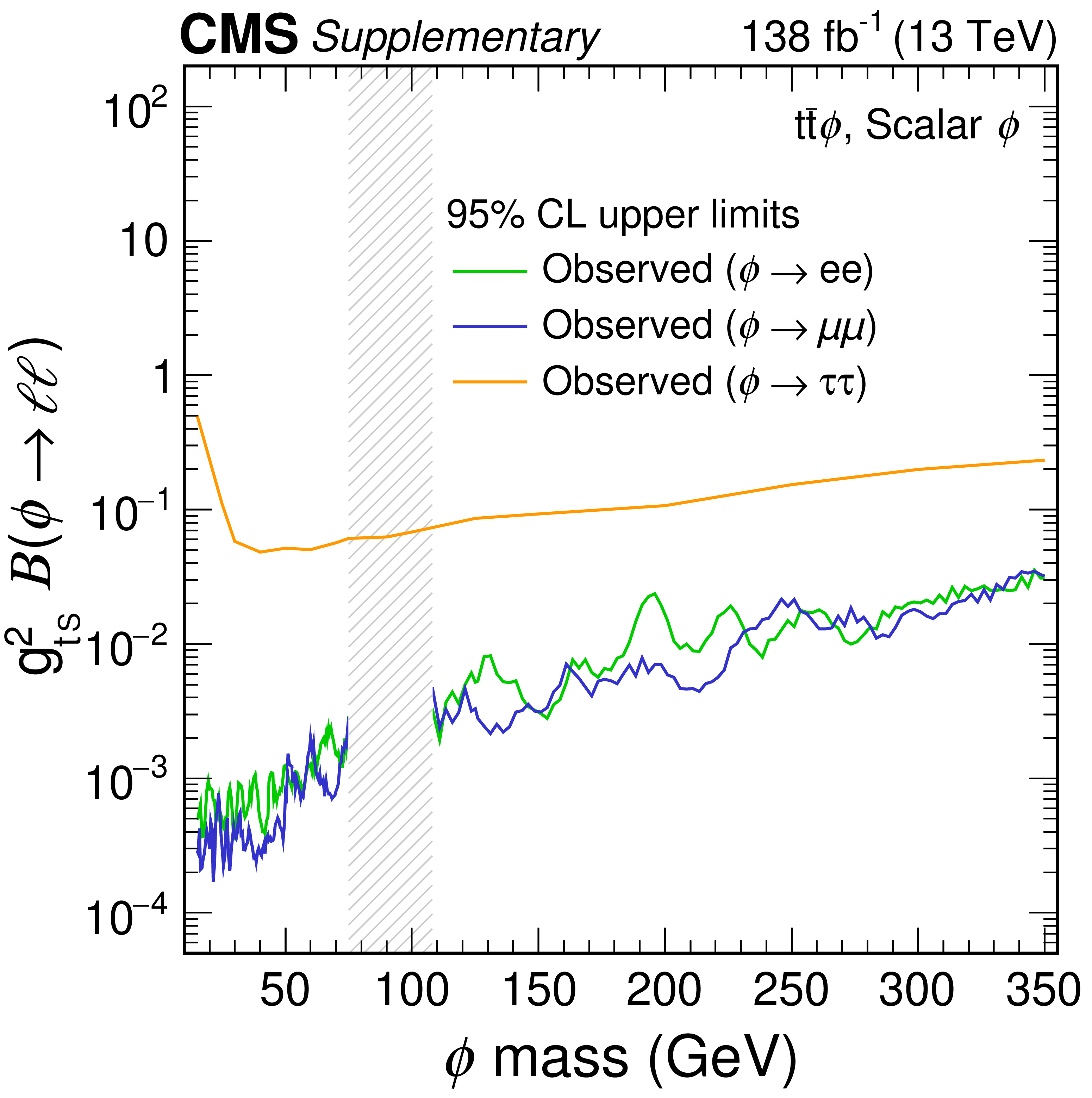
png pdf	Additional Figure 43: The 95% confidence level observed upper limits on the product of $ {\mathrm{g}}_{{\mathrm{t S}}}^2 $ and $ \mathcal{B}(\phi \to \ell\ell) $ of the $ {{\mathrm{t}\overline{\mathrm{t}}} }{\phi} $ signal with scalar couplings, where $ {\mathrm{g}}_{{\mathrm{t S}}} $ denotes the coupling of the $ \phi $ boson to the top quark and $ \mathcal{B}(\phi \to \ell\ell) $ is the branching fraction of the $ \phi $ boson into a lepton pair of given flavor. Exclusions on the dielectron, dimuon, and ditau decay scenarios of the $ \phi $ boson are shown with the green, blue, and orange solid lines, respectively. The vertical gray band indicates the mass region not considered in the analysis in the dielectron and dimuon decay scenarios of the $ \phi $ boson.
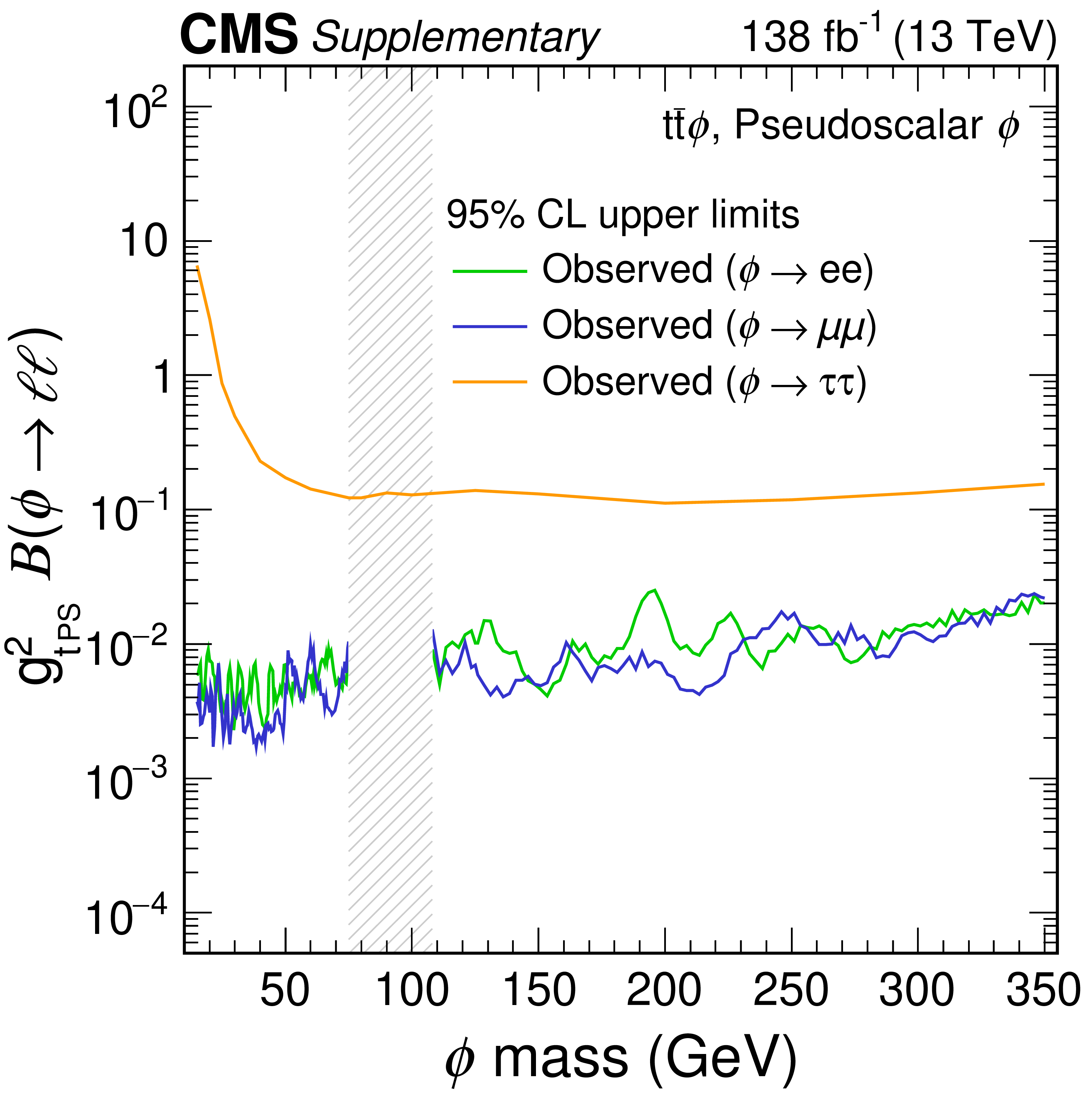
png pdf	Additional Figure 44: The 95% confidence level observed upper limits on the product of $ {\mathrm{g}}_{{\mathrm{t PS}}}^2 $ and $ \mathcal{B}(\phi \to \ell\ell) $ of the $ {{\mathrm{t}\overline{\mathrm{t}}} }{\phi} $ signal with pseudoscalar couplings, where $ {\mathrm{g}}_{{\mathrm{t PS}}} $ denotes the coupling of the $ \phi $ boson to the top quark and $ \mathcal{B}(\phi \to \ell\ell) $ is the branching fraction of the $ \phi $ boson into a lepton pair of given flavor. Exclusions on the dielectron, dimuon, and ditau decay scenarios of the $ \phi $ boson are shown with the green, blue, and orange solid lines, respectively. The vertical gray band indicates the mass region not considered in the analysis in the dielectron and dimuon decay scenarios of the $ \phi $ boson.
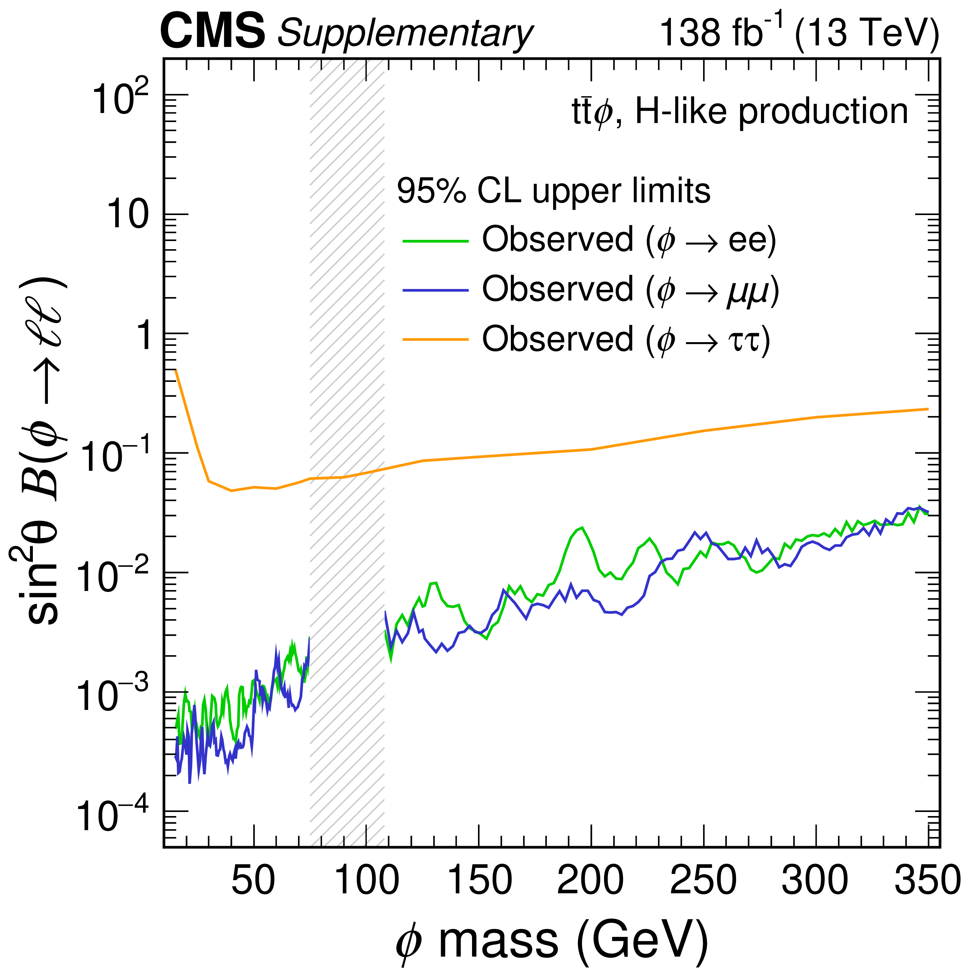
png pdf	Additional Figure 45: The 95% confidence level observed upper limits on the product of $ \sin^2\theta $ and $ \mathcal{B}(\phi \to \ell\ell) $ of the $ {{\mathrm{t}\overline{\mathrm{t}}} }{\phi} $ signal with H-like production, where $ \theta $ denotes the mixing angle of the Higgs boson with the $ \phi $ boson and $ \mathcal{B}(\phi \to \ell\ell) $ is the branching fraction of the $ \phi $ boson into a lepton pair of given flavor. Exclusions on the dielectron, dimuon, and ditau decay scenarios of the $ \phi $ boson are shown with the green, blue, and orange solid lines, respectively. The vertical gray band indicates the mass region not considered in the analysis in the dielectron and dimuon decay scenarios of the $ \phi $ boson.
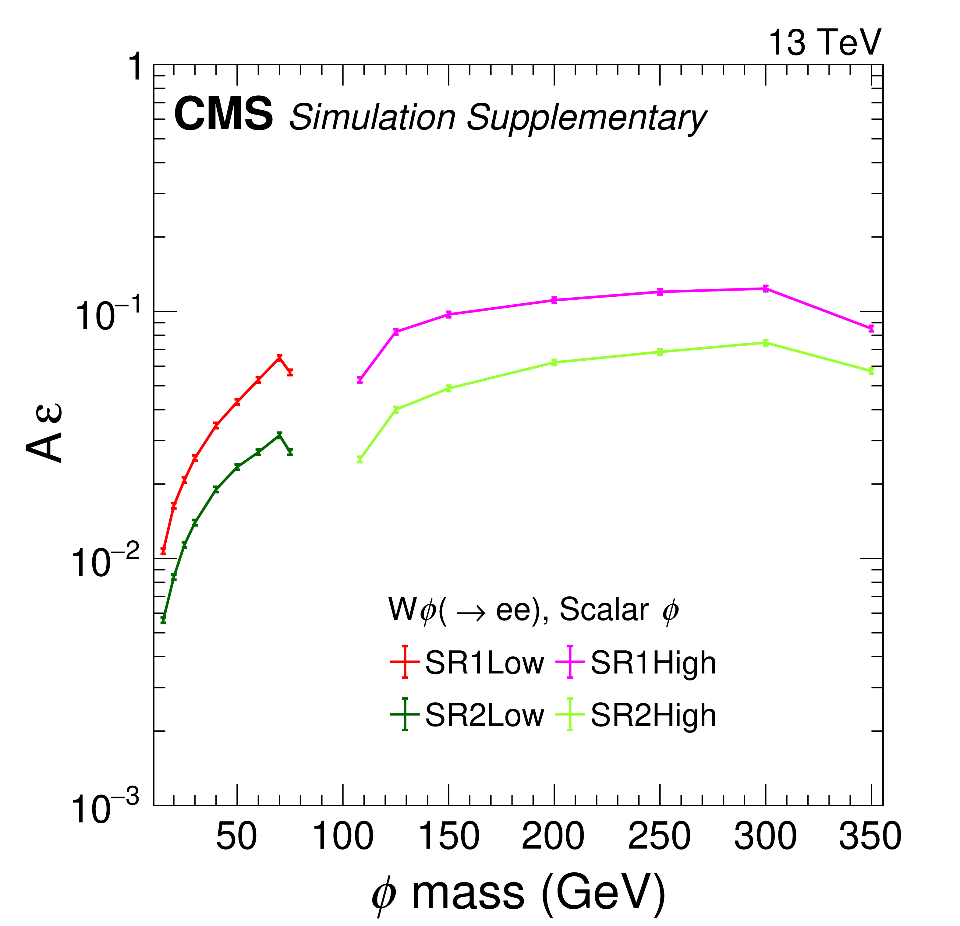
png pdf	Additional Figure 46: The product of acceptance and efficiency, $ {\mathrm{A}}\varepsilon $, for a scalar $ \phi $ boson in the $ {\mathrm{W}}{\phi} $ signal (with leptonic W decay) in each signal region in the dielectron decay scenario. Each value is computed as the ratio of the number of simulated signal events passing all selection criteria to the total number of simulated signal events, and includes the data-to-simulation correction factors described in the paper.
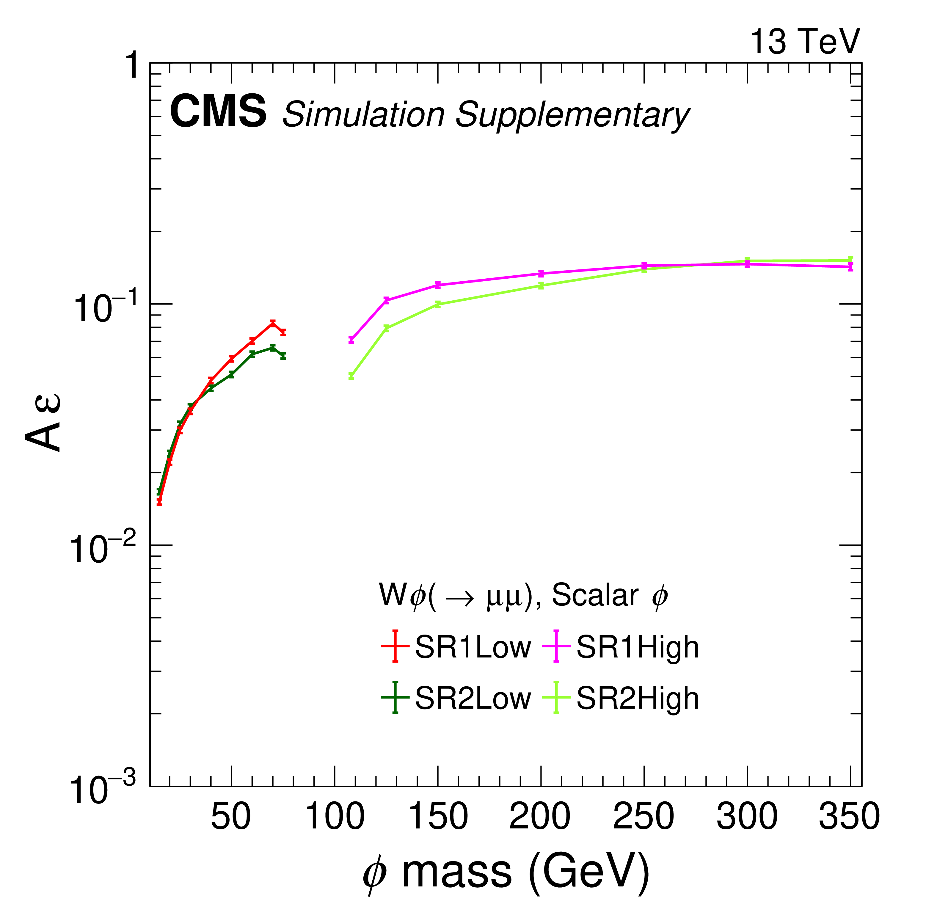
png pdf	Additional Figure 47: The product of acceptance and efficiency, $ {\mathrm{A}}\varepsilon $, for a scalar $ \phi $ boson in the $ {\mathrm{W}}{\phi} $ signal (with leptonic W decay) in each signal region in the dimuon decay scenario. Each value is computed as the ratio of the number of simulated signal events passing all selection criteria to the total number of simulated signal events, and includes the data-to-simulation correction factors described in the paper.
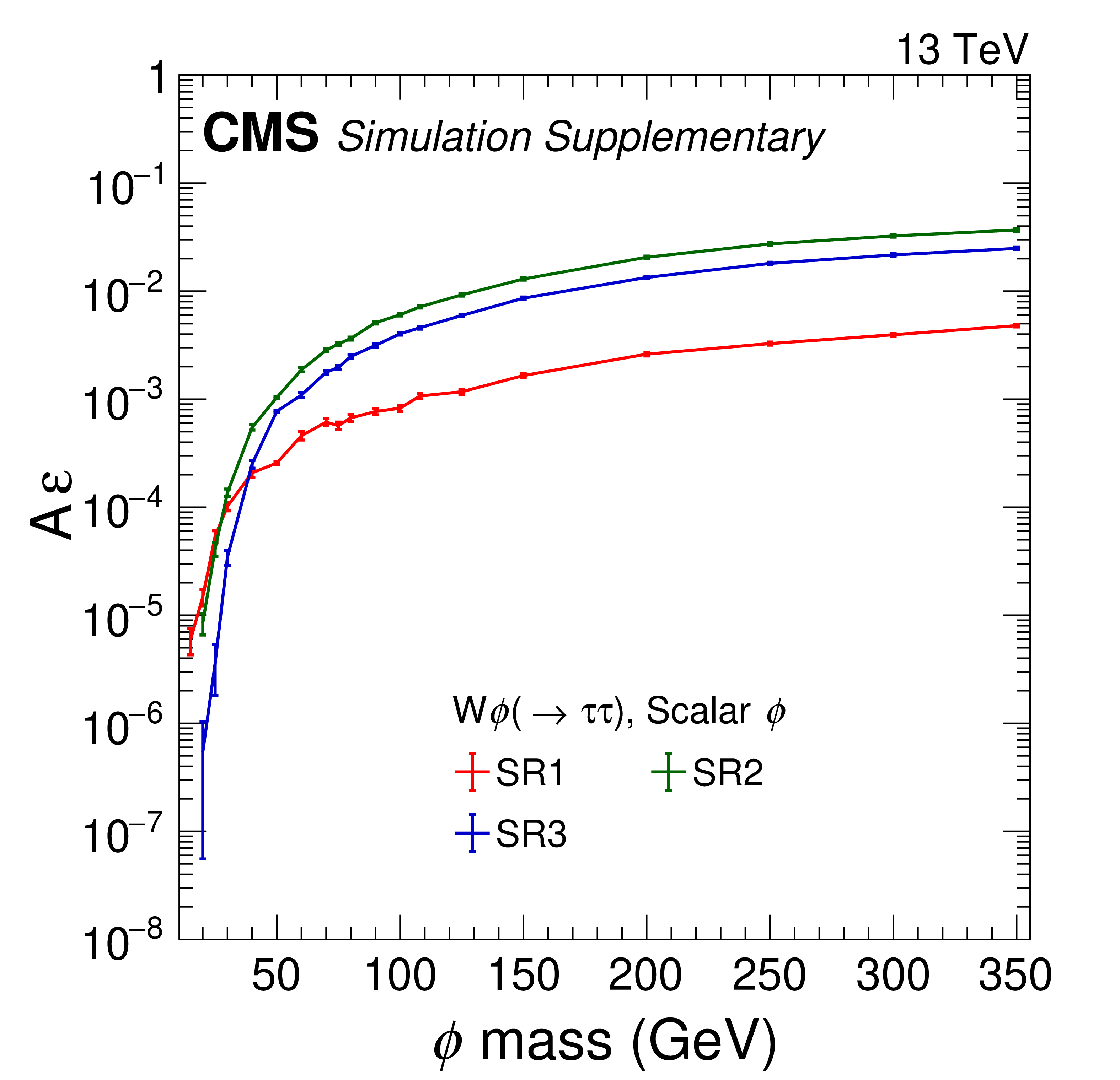
png pdf	Additional Figure 48: The product of acceptance and efficiency, $ {\mathrm{A}}\varepsilon $, for a scalar $ \phi $ boson in the $ {\mathrm{W}}{\phi} $ signal (with leptonic W decay) in each signal region in the ditau decay scenario. Each value is computed as the ratio of the number of simulated signal events passing all selection criteria to the total number of simulated signal events, and includes the data-to-simulation correction factors described in the paper.
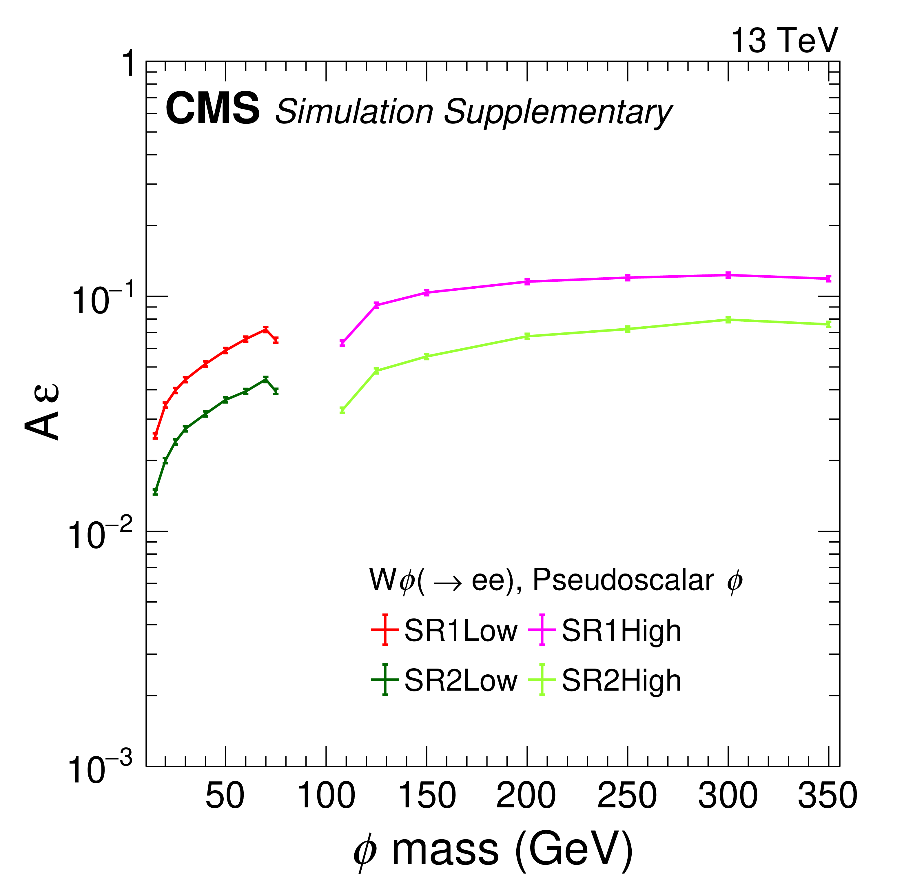
png pdf	Additional Figure 49: The product of acceptance and efficiency, $ {\mathrm{A}}\varepsilon $, for a pseudoscalar $ \phi $ boson in the $ {\mathrm{W}}{\phi} $ signal (with leptonic W decay) in each signal region in the dielectron decay scenario. Each value is computed as the ratio of the number of simulated signal events passing all selection criteria to the total number of simulated signal events, and includes the data-to-simulation correction factors described in the paper.
png pdf	Additional Figure 50: The product of acceptance and efficiency, $ {\mathrm{A}}\varepsilon $, for a pseudoscalar $ \phi $ boson in the $ {\mathrm{W}}{\phi} $ signal (with leptonic W decay) in each signal region in the dimuon decay scenario. Each value is computed as the ratio of the number of simulated signal events passing all selection criteria to the total number of simulated signal events, and includes the data-to-simulation correction factors described in the paper.
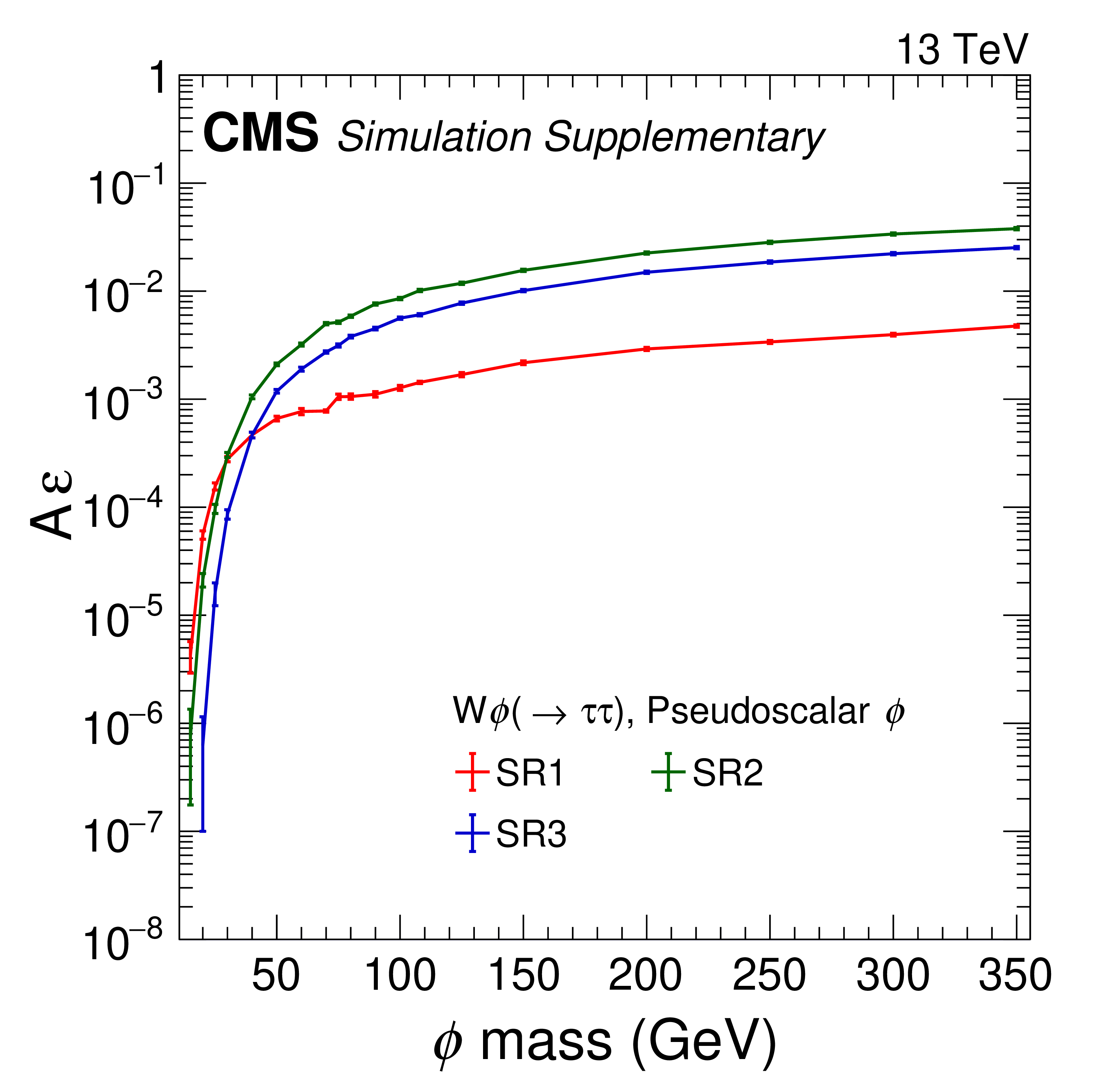
png pdf	Additional Figure 51: The product of acceptance and efficiency, $ {\mathrm{A}}\varepsilon $, for a pseudoscalar $ \phi $ boson in the $ {\mathrm{W}}{\phi} $ signal (with leptonic W decay) in each signal region in the ditau decay scenario. Each value is computed as the ratio of the number of simulated signal events passing all selection criteria to the total number of simulated signal events, and includes the data-to-simulation correction factors described in the paper.
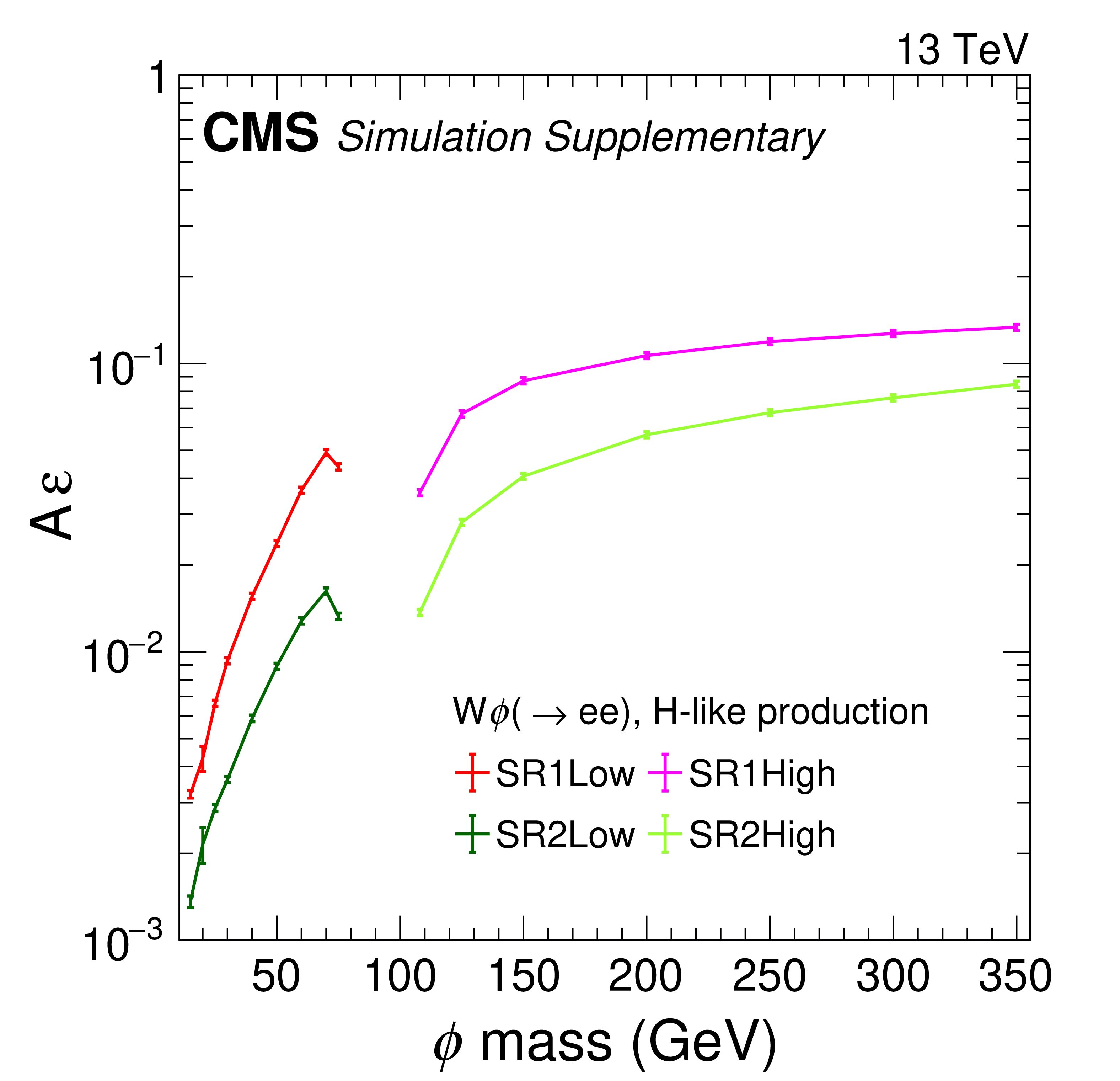
png pdf	Additional Figure 52: The product of acceptance and efficiency, $ {\mathrm{A}}\varepsilon $, for an H-like $ \phi $ boson in the $ {\mathrm{W}}{\phi} $ signal (with leptonic W decay) in each signal region in the dielectron decay scenario. Each value is computed as the ratio of the number of simulated signal events passing all selection criteria to the total number of simulated signal events, and includes the data-to-simulation correction factors described in the paper.
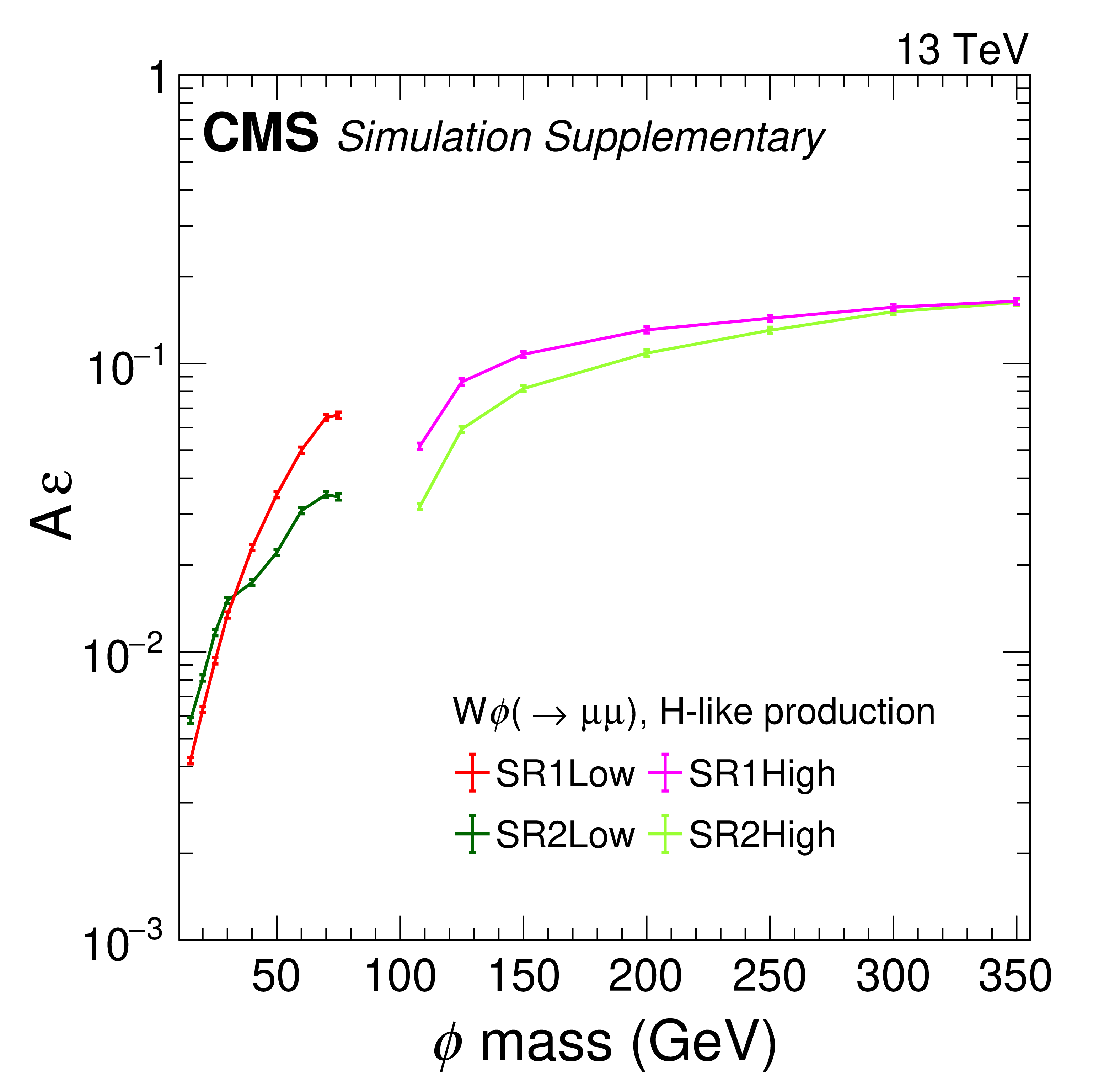
png pdf	Additional Figure 53: The product of acceptance and efficiency, $ {\mathrm{A}}\varepsilon $, for an H-like $ \phi $ boson in the $ {\mathrm{W}}{\phi} $ signal (with leptonic W decay) in each signal region in the dimuon decay scenario. Each value is computed as the ratio of the number of simulated signal events passing all selection criteria to the total number of simulated signal events, and includes the data-to-simulation correction factors described in the paper.
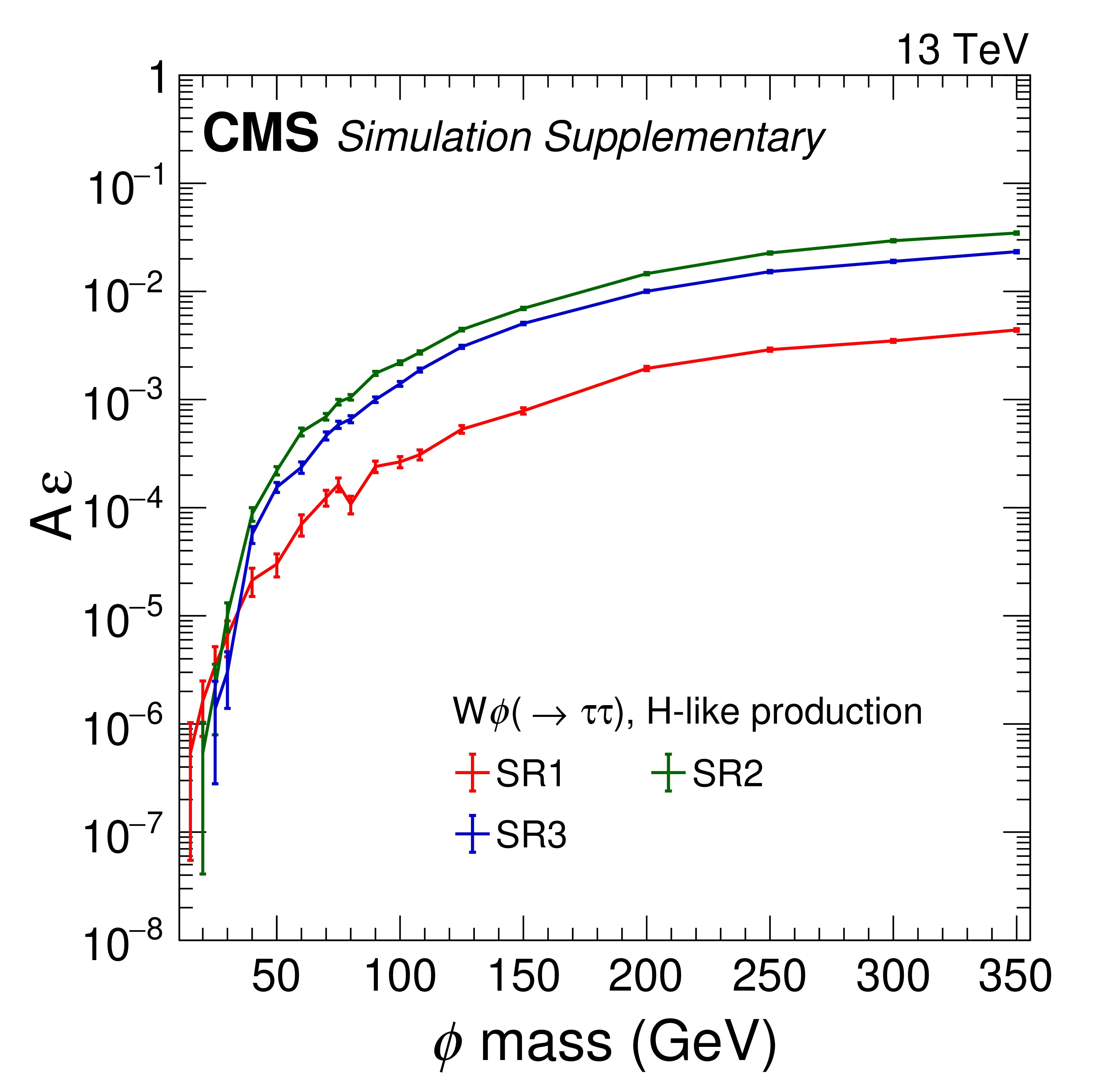
png pdf	Additional Figure 54: The product of acceptance and efficiency, $ {\mathrm{A}}\varepsilon $, for an H-like $ \phi $ boson in the $ {\mathrm{W}}{\phi} $ signal (with leptonic W decay) in each signal region in the ditau decay scenario. Each value is computed as the ratio of the number of simulated signal events passing all selection criteria to the total number of simulated signal events, and includes the data-to-simulation correction factors described in the paper.
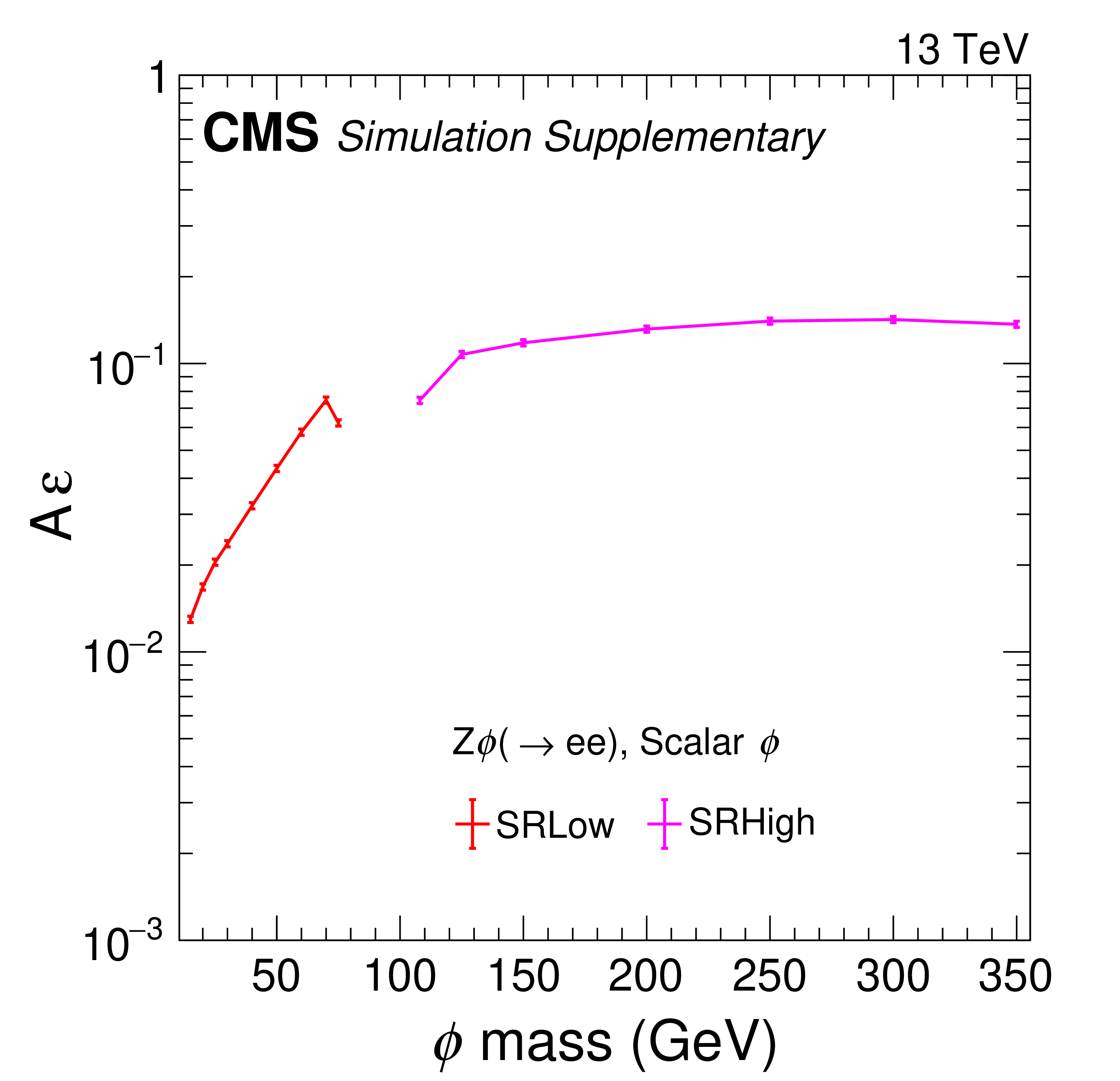
png pdf	Additional Figure 55: The product of acceptance and efficiency, $ {\mathrm{A}}\varepsilon $, for a scalar $ \phi $ boson in the $ {\mathrm{Z}}{\phi} $ signal (with leptonic Z decay) in each signal region in the dielectron decay scenario. Each value is computed as the ratio of the number of simulated signal events passing all selection criteria to the total number of simulated signal events, and includes the data-to-simulation correction factors described in the paper.
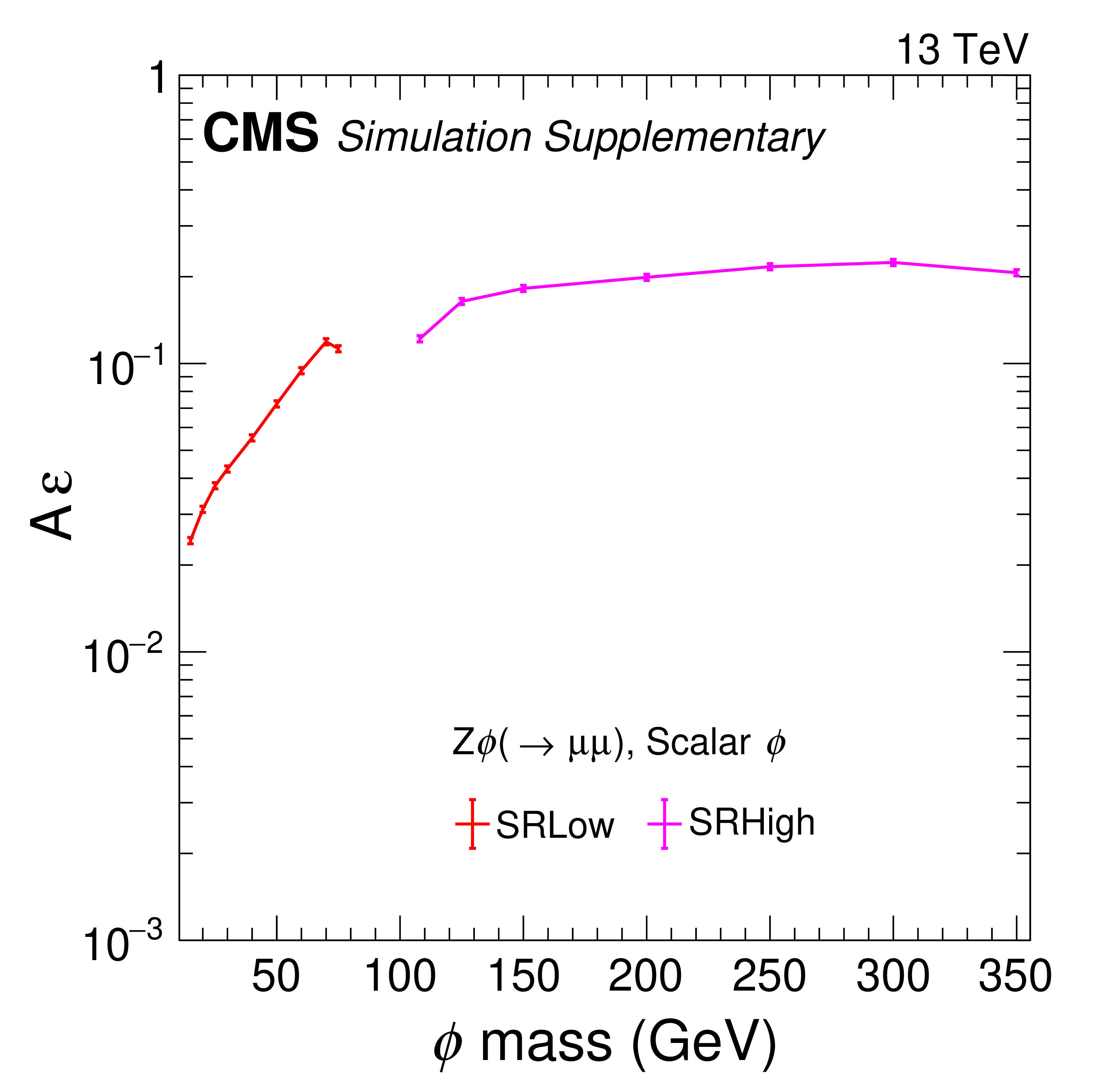
png pdf	Additional Figure 56: The product of acceptance and efficiency, $ {\mathrm{A}}\varepsilon $, for a scalar $ \phi $ boson in the $ {\mathrm{Z}}{\phi} $ signal (with leptonic Z decay) in each signal region in the dimuon decay scenario. Each value is computed as the ratio of the number of simulated signal events passing all selection criteria to the total number of simulated signal events, and includes the data-to-simulation correction factors described in the paper.
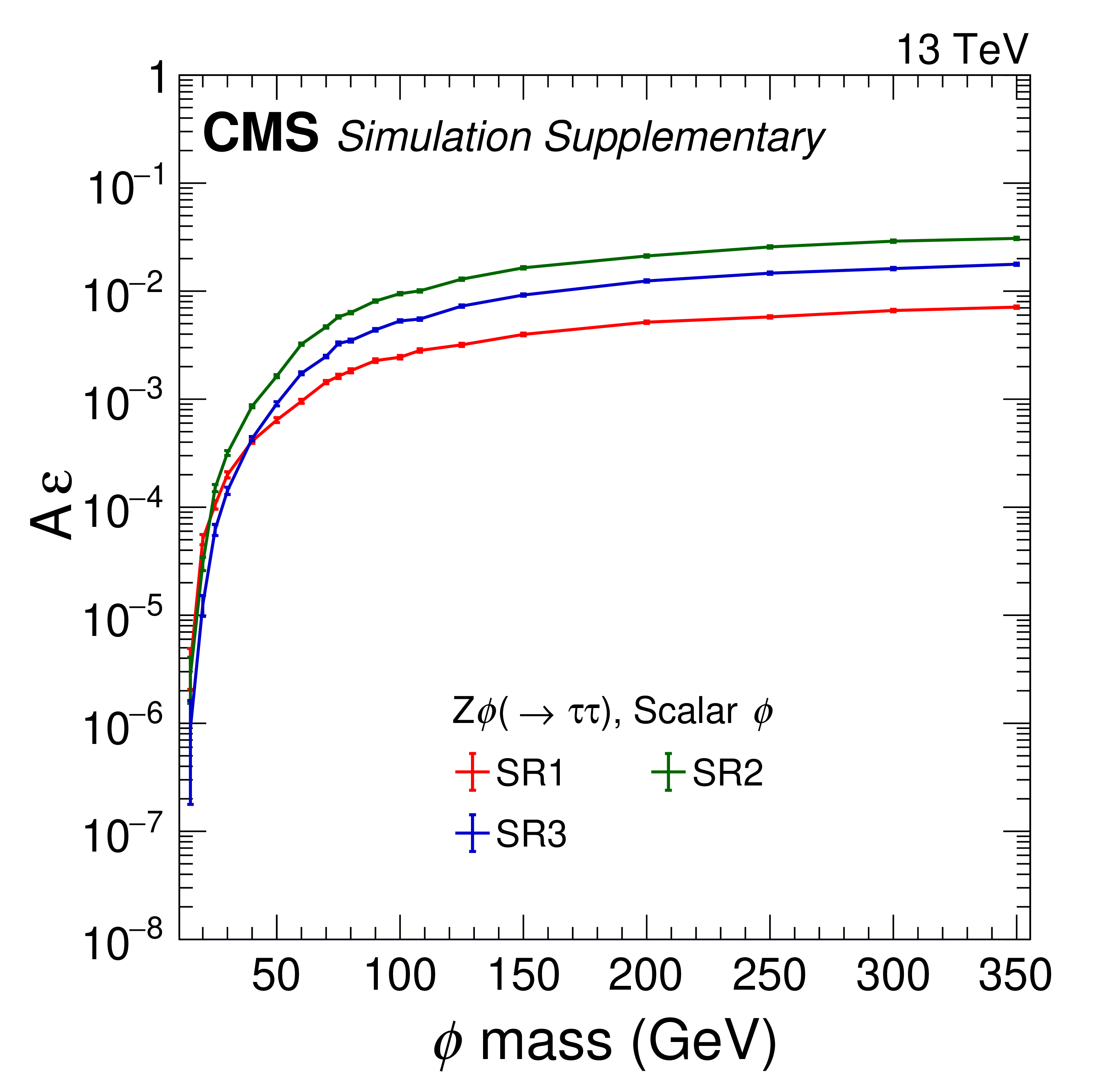
png pdf	Additional Figure 57: The product of acceptance and efficiency, $ {\mathrm{A}}\varepsilon $, for a scalar $ \phi $ boson in the $ {\mathrm{Z}}{\phi} $ signal (with leptonic Z decay) in each signal region in the ditau decay scenario. Each value is computed as the ratio of the number of simulated signal events passing all selection criteria to the total number of simulated signal events, and includes the data-to-simulation correction factors described in the paper.
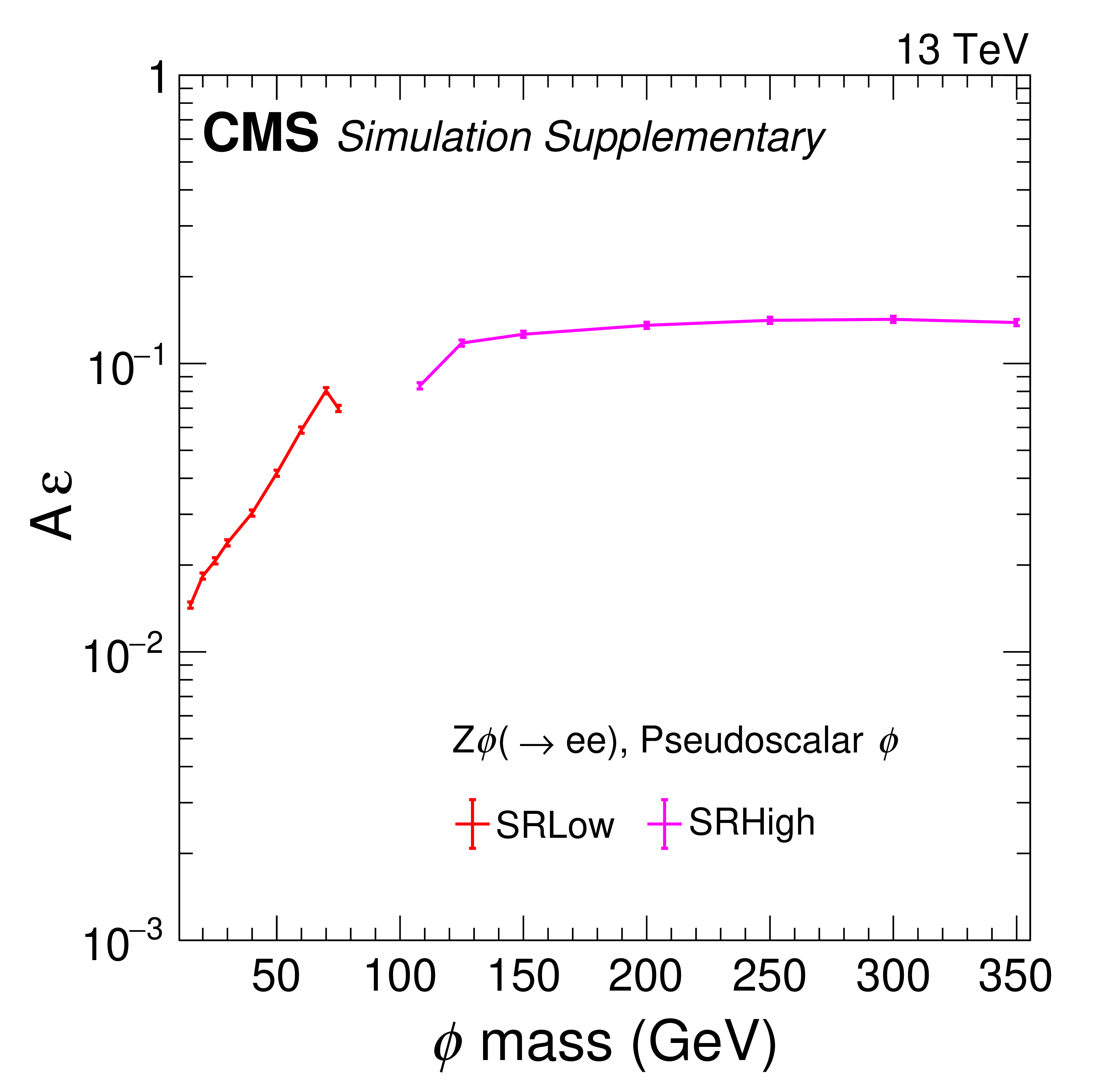
png pdf	Additional Figure 58: The product of acceptance and efficiency, $ {\mathrm{A}}\varepsilon $, for a pseudoscalar $ \phi $ boson in the $ {\mathrm{Z}}{\phi} $ signal (with leptonic Z decay) in each signal region in the dielectron decay scenario. Each value is computed as the ratio of the number of simulated signal events passing all selection criteria to the total number of simulated signal events, and includes the data-to-simulation correction factors described in the paper.
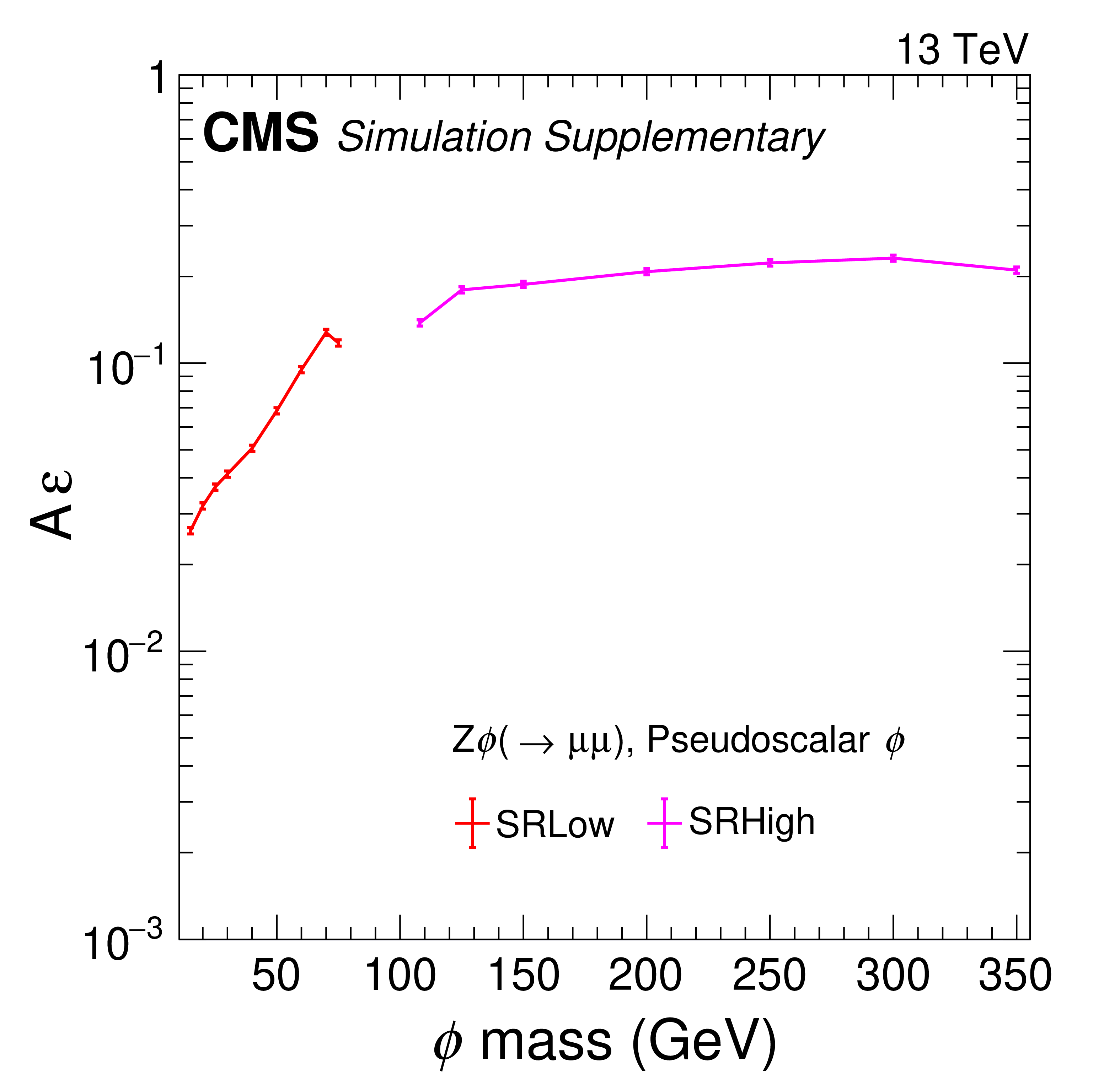
png pdf	Additional Figure 59: The product of acceptance and efficiency, $ {\mathrm{A}}\varepsilon $, for a pseudoscalar $ \phi $ boson in the $ {\mathrm{Z}}{\phi} $ signal (with leptonic Z decay) in each signal region in the dimuon decay scenario. Each value is computed as the ratio of the number of simulated signal events passing all selection criteria to the total number of simulated signal events, and includes the data-to-simulation correction factors described in the paper.
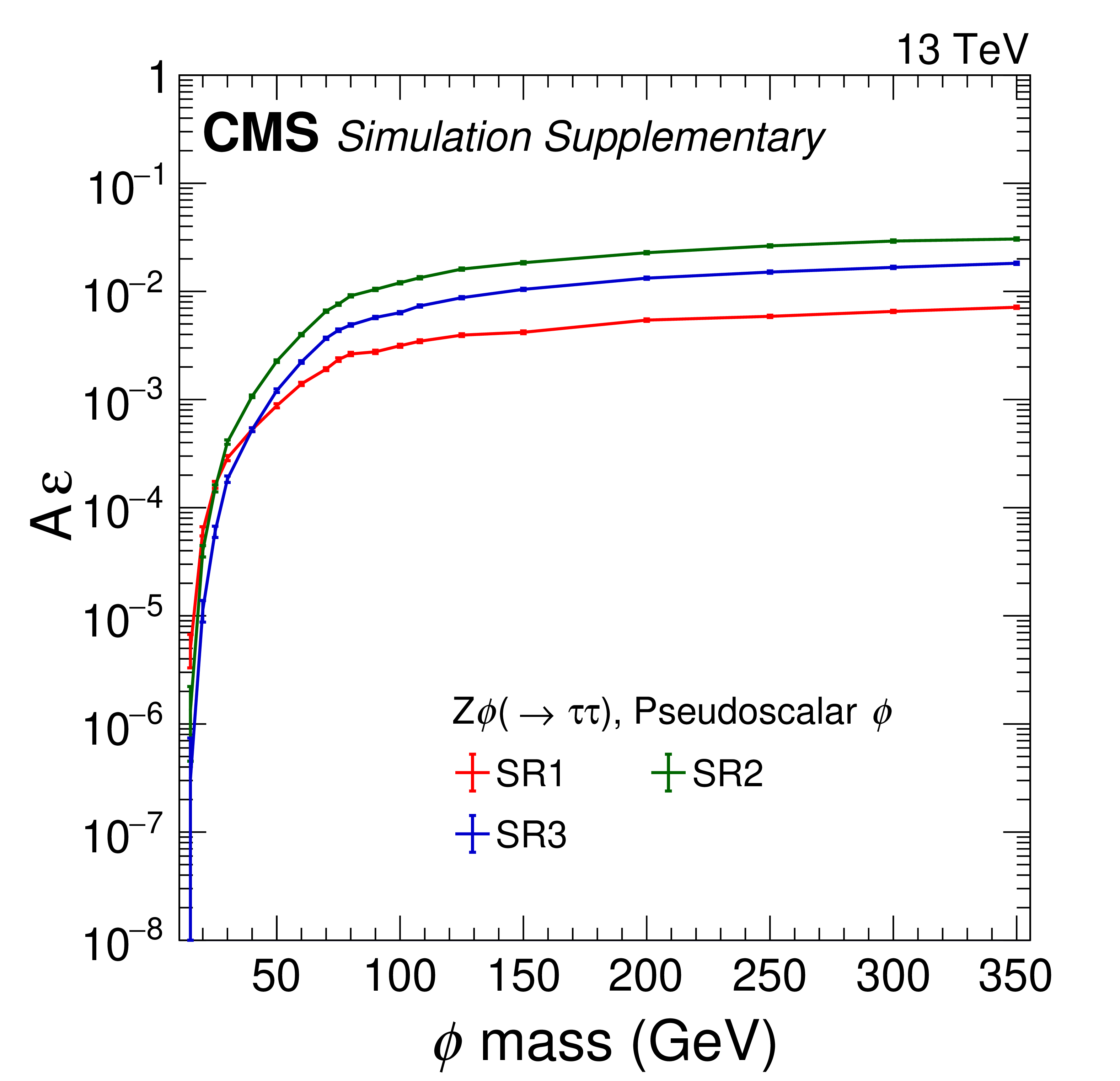
png pdf	Additional Figure 60: The product of acceptance and efficiency, $ {\mathrm{A}}\varepsilon $, for a pseudoscalar $ \phi $ boson in the $ {\mathrm{Z}}{\phi} $ signal (with leptonic Z decay) in each signal region in the ditau decay scenario. Each value is computed as the ratio of the number of simulated signal events passing all selection criteria to the total number of simulated signal events, and includes the data-to-simulation correction factors described in the paper.
png pdf	Additional Figure 61: The product of acceptance and efficiency, $ {\mathrm{A}}\varepsilon $, for an H-like $ \phi $ boson in the $ {\mathrm{Z}}{\phi} $ signal (with leptonic Z decay) in each signal region in the dielectron decay scenario. Each value is computed as the ratio of the number of simulated signal events passing all selection criteria to the total number of simulated signal events, and includes the data-to-simulation correction factors described in the paper.
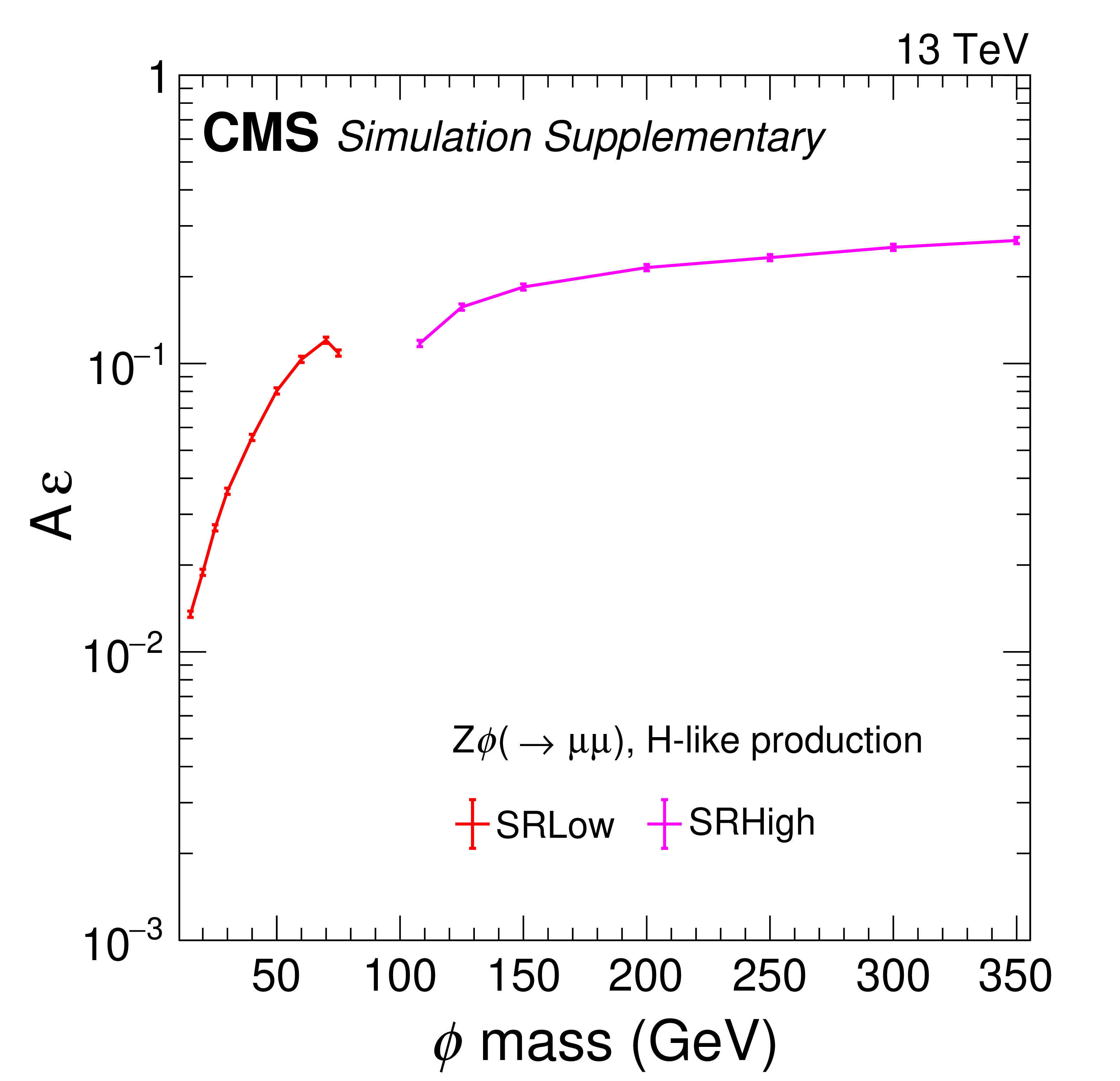
png pdf	Additional Figure 62: The product of acceptance and efficiency, $ {\mathrm{A}}\varepsilon $, for an H-like $ \phi $ boson in the $ {\mathrm{Z}}{\phi} $ signal (with leptonic Z decay) in each signal region in the dimuon decay scenario. Each value is computed as the ratio of the number of simulated signal events passing all selection criteria to the total number of simulated signal events, and includes the data-to-simulation correction factors described in the paper.
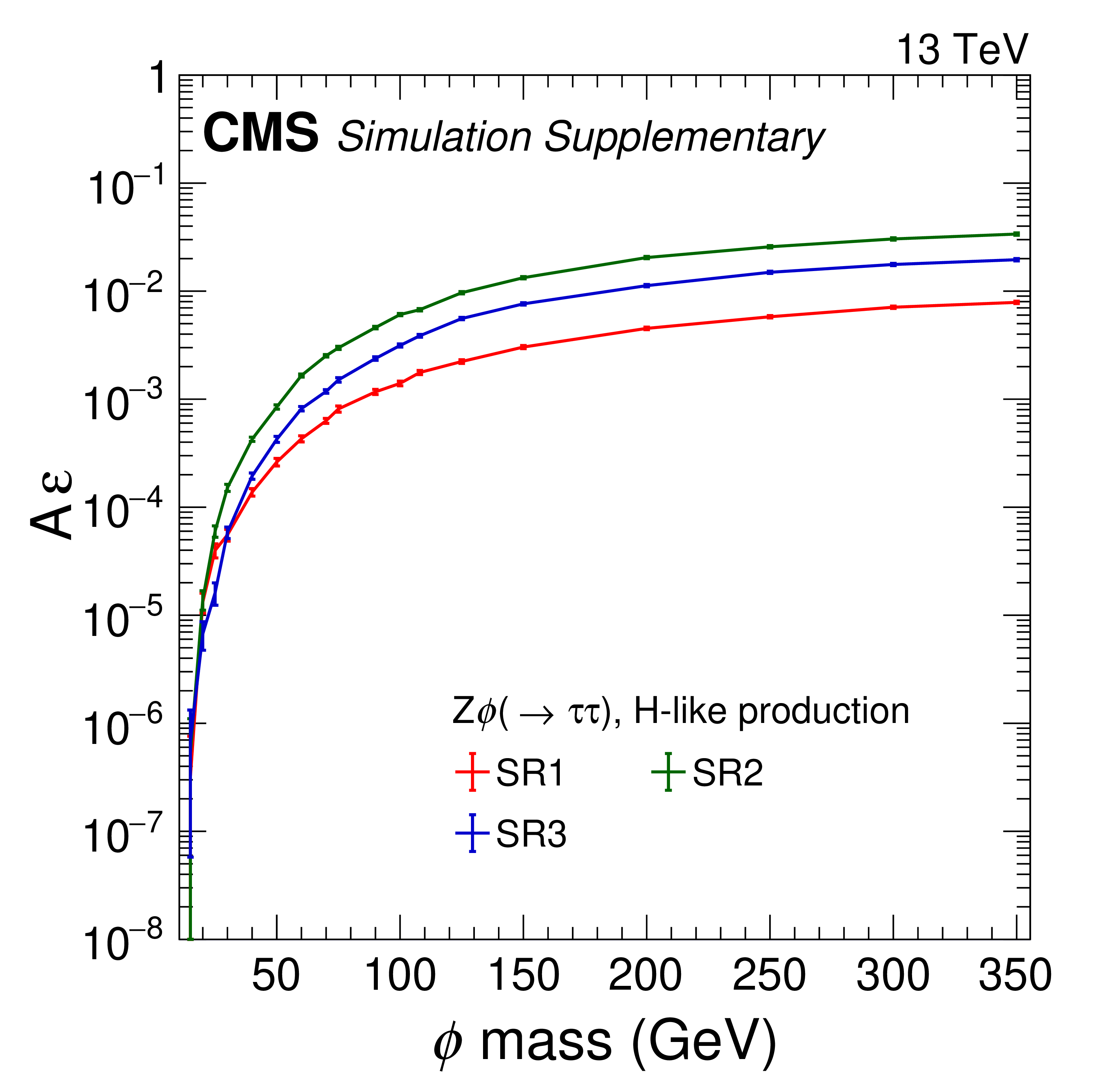
png pdf	Additional Figure 63: The product of acceptance and efficiency, $ {\mathrm{A}}\varepsilon $, for an H-like $ \phi $ boson in the $ {\mathrm{Z}}{\phi} $ signal (with leptonic Z decay) in each signal region in the ditau decay scenario. Each value is computed as the ratio of the number of simulated signal events passing all selection criteria to the total number of simulated signal events, and includes the data-to-simulation correction factors described in the paper.
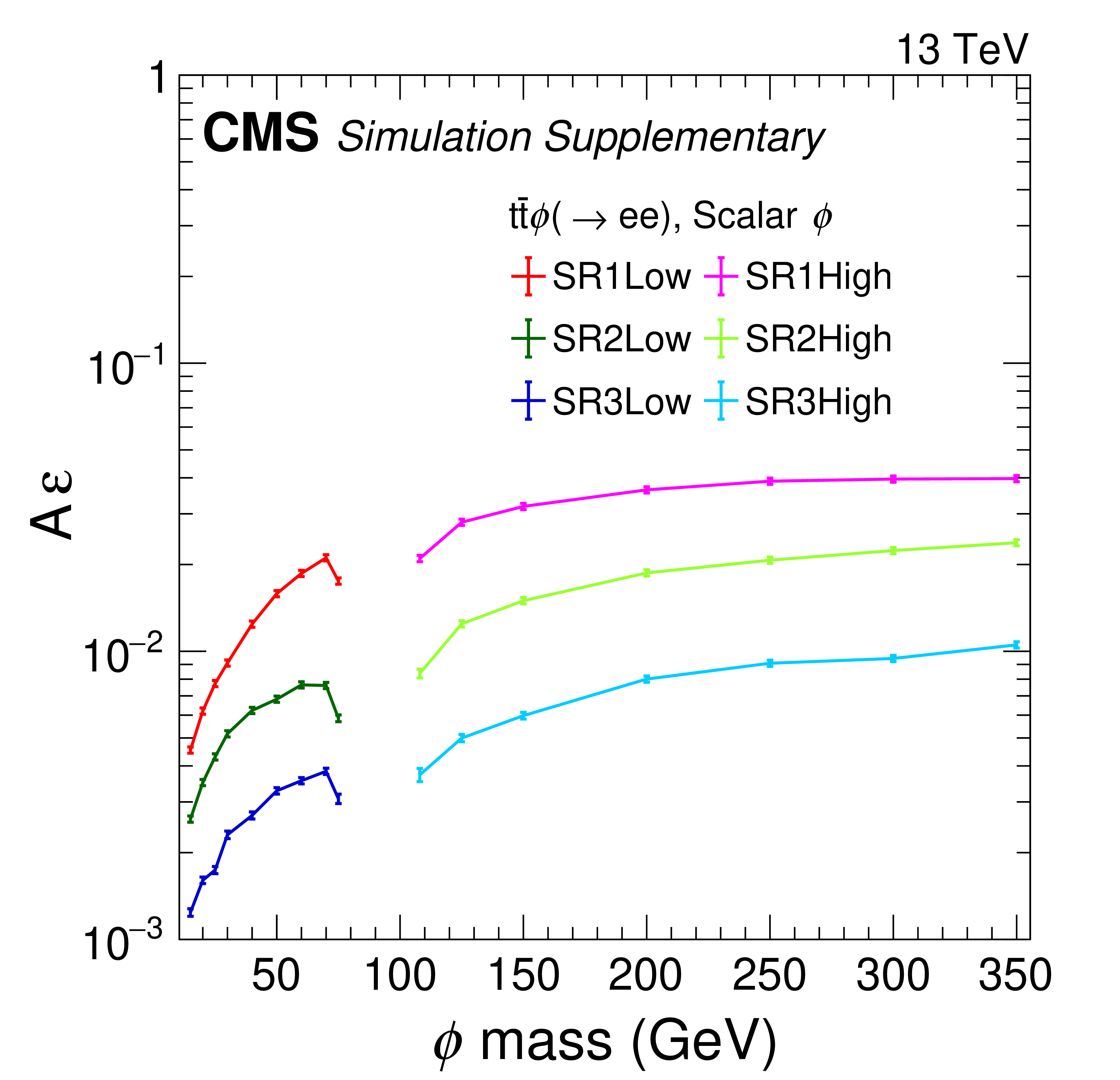
png pdf	Additional Figure 64: The product of acceptance and efficiency, $ {\mathrm{A}}\varepsilon $, for a scalar $ \phi $ boson in the $ {{\mathrm{t}\overline{\mathrm{t}}} }{\phi} $ signal (with inclusive $ {\mathrm{t}\overline{\mathrm{t}}} $ decay) in each signal region in the dielectron decay scenario. Each value is computed as the ratio of the number of simulated signal events passing all selection criteria to the total number of simulated signal events, and includes the data-to-simulation correction factors described in the paper.
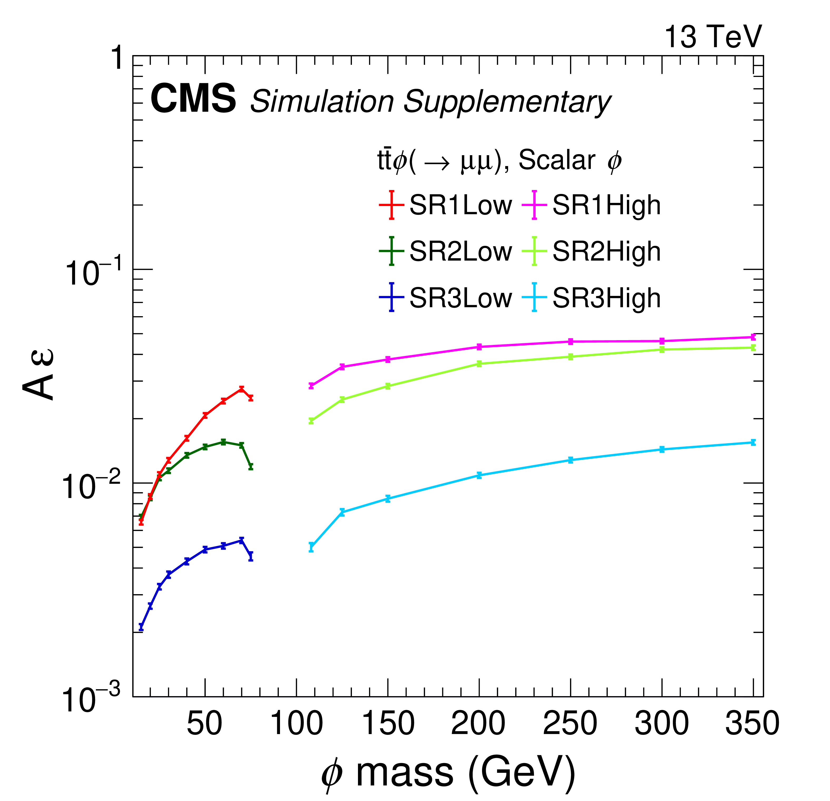
png pdf	Additional Figure 65: The product of acceptance and efficiency, $ {\mathrm{A}}\varepsilon $, for a scalar $ \phi $ boson in the $ {{\mathrm{t}\overline{\mathrm{t}}} }{\phi} $ signal (with inclusive $ {\mathrm{t}\overline{\mathrm{t}}} $ decay) in each signal region in the dimuon decay scenario. Each value is computed as the ratio of the number of simulated signal events passing all selection criteria to the total number of simulated signal events, and includes the data-to-simulation correction factors described in the paper.
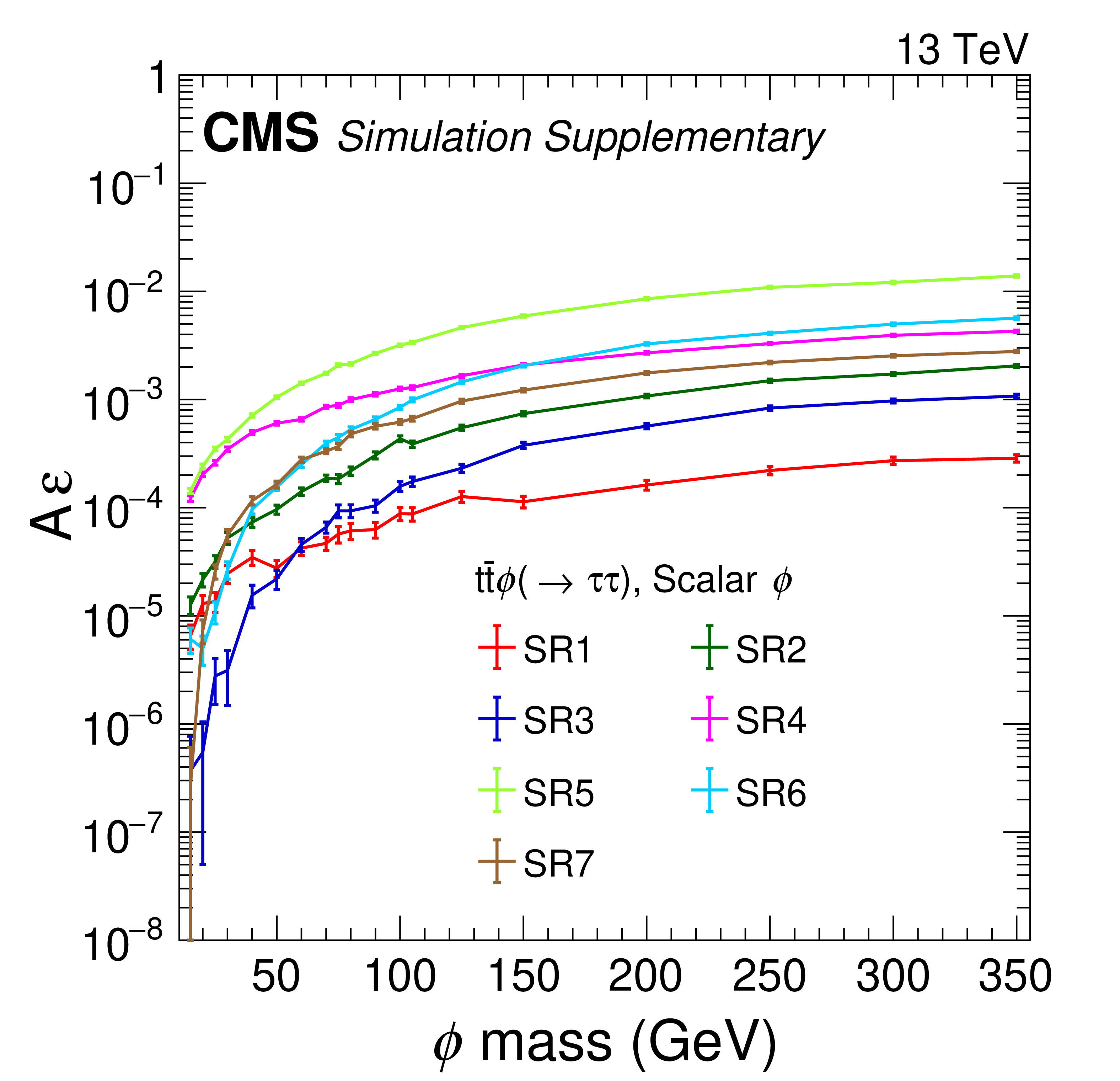
png pdf	Additional Figure 66: The product of acceptance and efficiency, $ {\mathrm{A}}\varepsilon $, for a scalar $ \phi $ boson in the $ {{\mathrm{t}\overline{\mathrm{t}}} }{\phi} $ signal (with inclusive $ {\mathrm{t}\overline{\mathrm{t}}} $ decay) in each signal region in the ditau decay scenario. Each value is computed as the ratio of the number of simulated signal events passing all selection criteria to the total number of simulated signal events, and includes the data-to-simulation correction factors described in the paper.
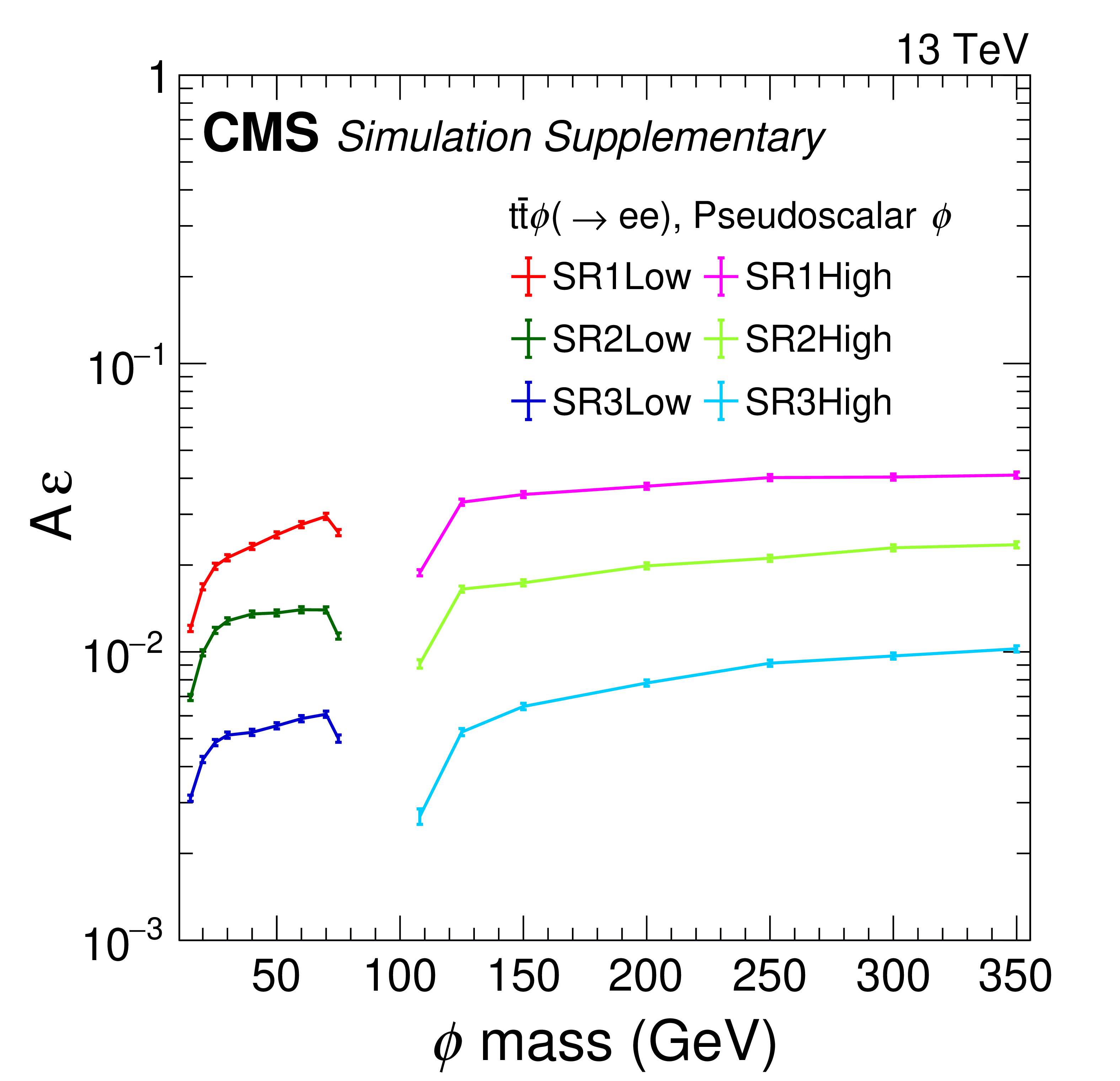
png pdf	Additional Figure 67: The product of acceptance and efficiency, $ {\mathrm{A}}\varepsilon $, for a pseudoscalar $ \phi $ boson in the $ {{\mathrm{t}\overline{\mathrm{t}}} }{\phi} $ signal (with inclusive $ {\mathrm{t}\overline{\mathrm{t}}} $ decay) in each signal region in the dielectron decay scenario. Each value is computed as the ratio of the number of simulated signal events passing all selection criteria to the total number of simulated signal events, and includes the data-to-simulation correction factors described in the paper.
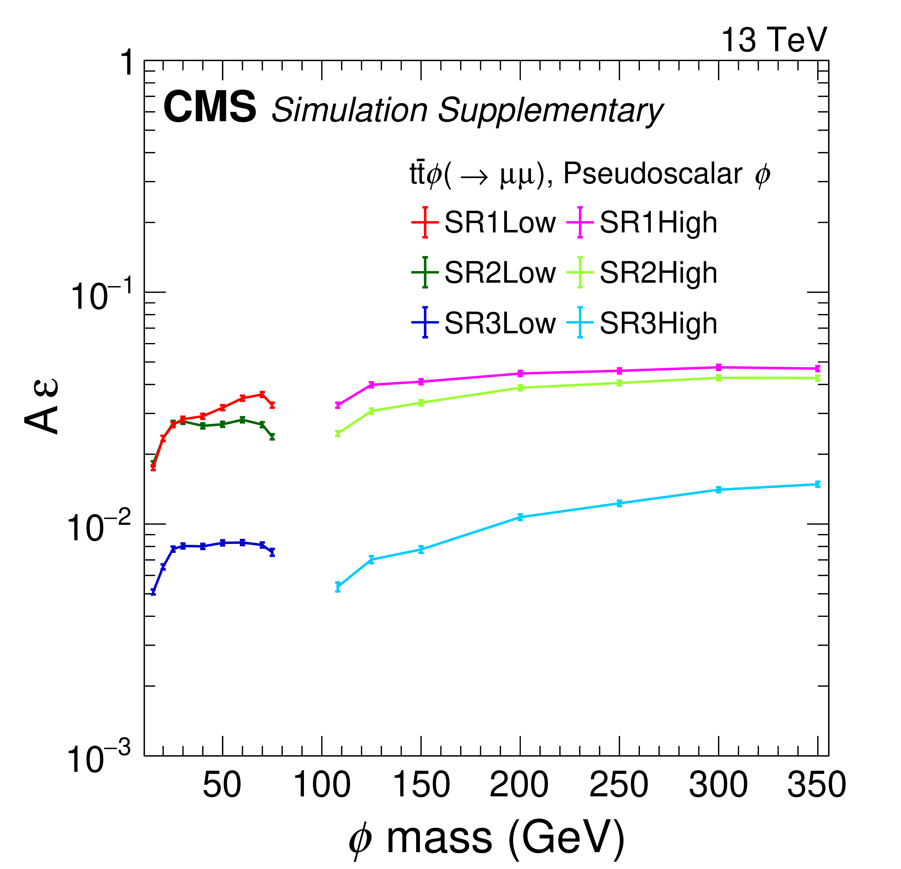
png pdf	Additional Figure 68: The product of acceptance and efficiency, $ {\mathrm{A}}\varepsilon $, for a pseudoscalar $ \phi $ boson in the $ {{\mathrm{t}\overline{\mathrm{t}}} }{\phi} $ signal (with inclusive $ {\mathrm{t}\overline{\mathrm{t}}} $ decay) in each signal region in the dimuon decay scenario. Each value is computed as the ratio of the number of simulated signal events passing all selection criteria to the total number of simulated signal events, and includes the data-to-simulation correction factors described in the paper.
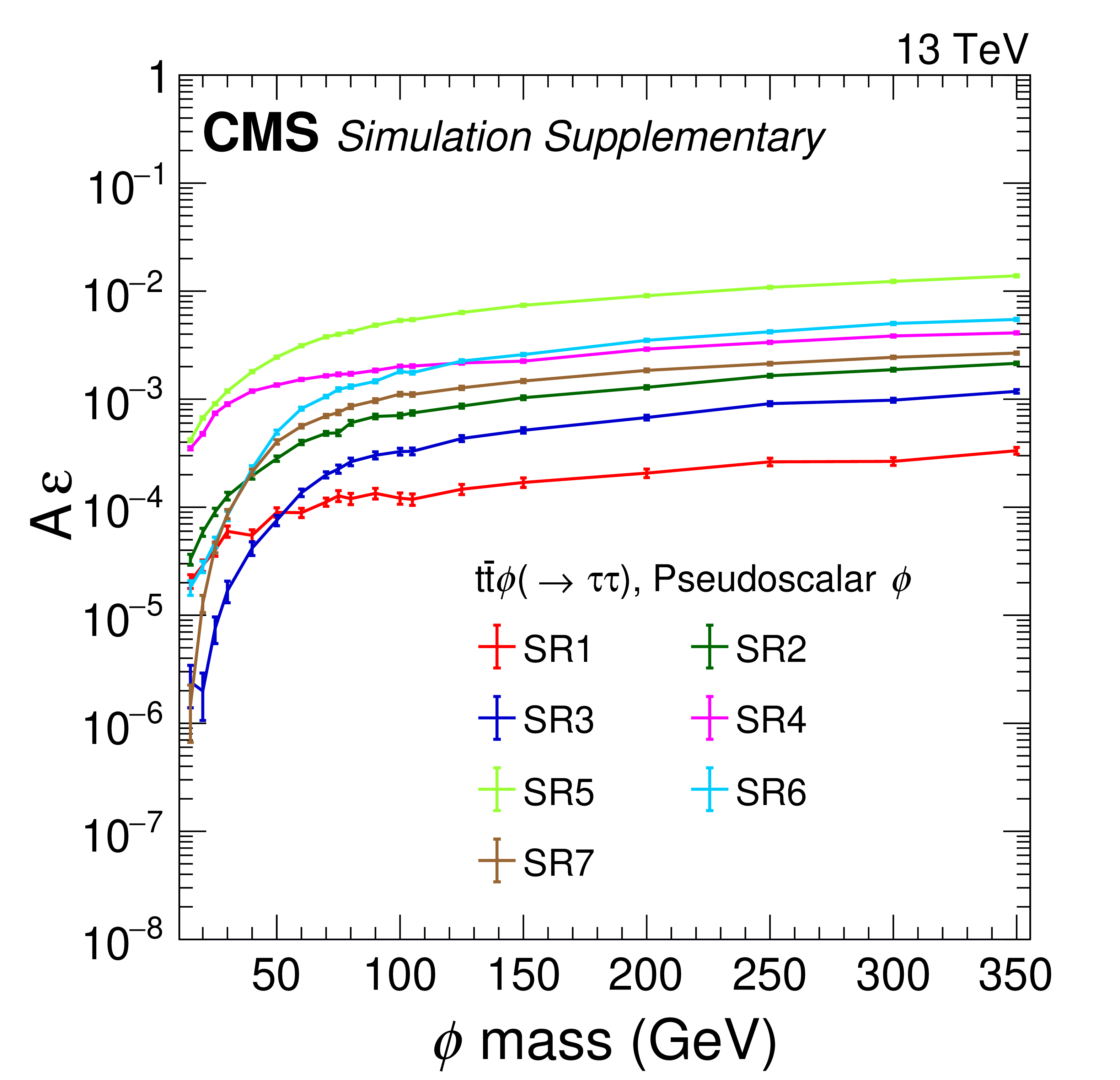
png pdf	Additional Figure 69: The product of acceptance and efficiency, $ {\mathrm{A}}\varepsilon $, for a pseudoscalar $ \phi $ boson in the $ {{\mathrm{t}\overline{\mathrm{t}}} }{\phi} $ signal (with inclusive $ {\mathrm{t}\overline{\mathrm{t}}} $ decay) in each signal region in the ditau decay scenario. Each value is computed as the ratio of the number of simulated signal events passing all selection criteria to the total number of simulated signal events, and includes the data-to-simulation correction factors described in the paper.
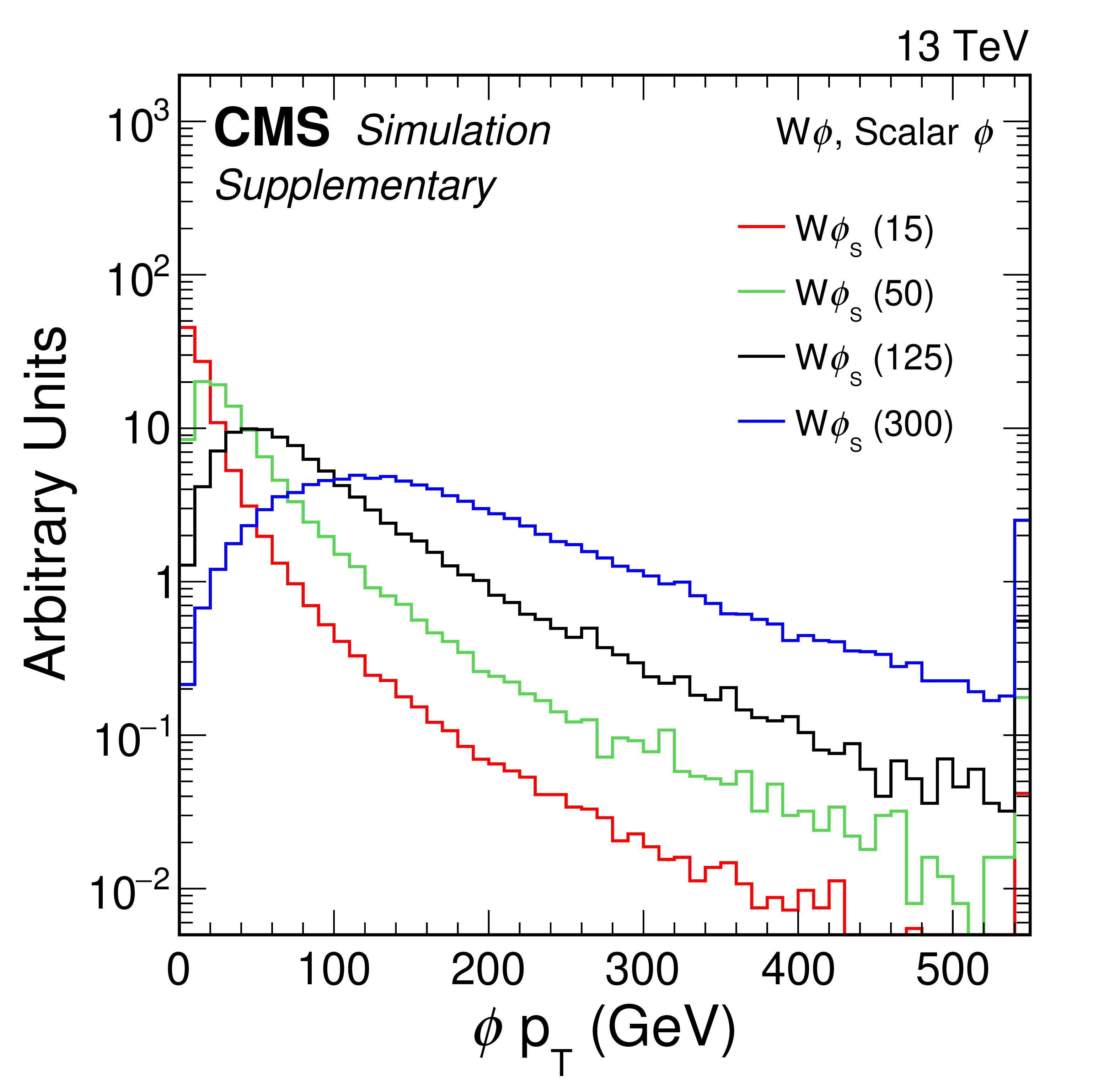
png pdf	Additional Figure 70: Generator level transverse momentum, $ p_{\mathrm{T}} $, of the $ \phi $ boson in the $ {\mathrm{W}}{\phi} $ signal with scalar couplings. Histograms are provided for several $ \phi $ masses as indicated in units of GeV, and are normalized to the same integral value. The rightmost bin contains the overflow events in each distribution.
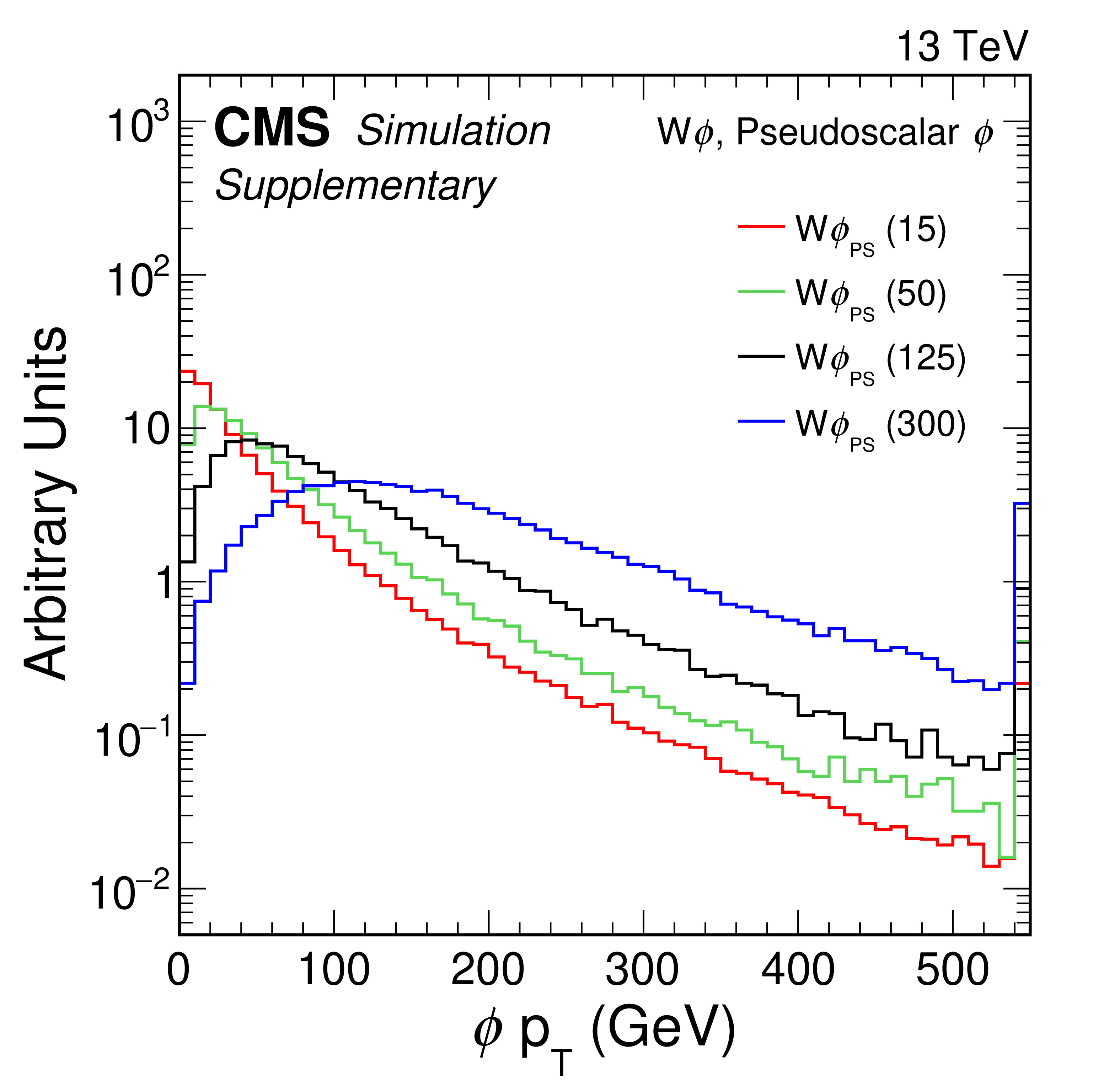
png pdf	Additional Figure 71: Generator level transverse momentum, $ p_{\mathrm{T}} $, of $ \phi $ boson in the $ {\mathrm{W}}{\phi} $ signal with pseudoscalar couplings. Histograms are provided for several $ \phi $ masses as indicated in units of GeV, and are normalized to the same integral value. The rightmost bin contains the overflow events in each distribution.
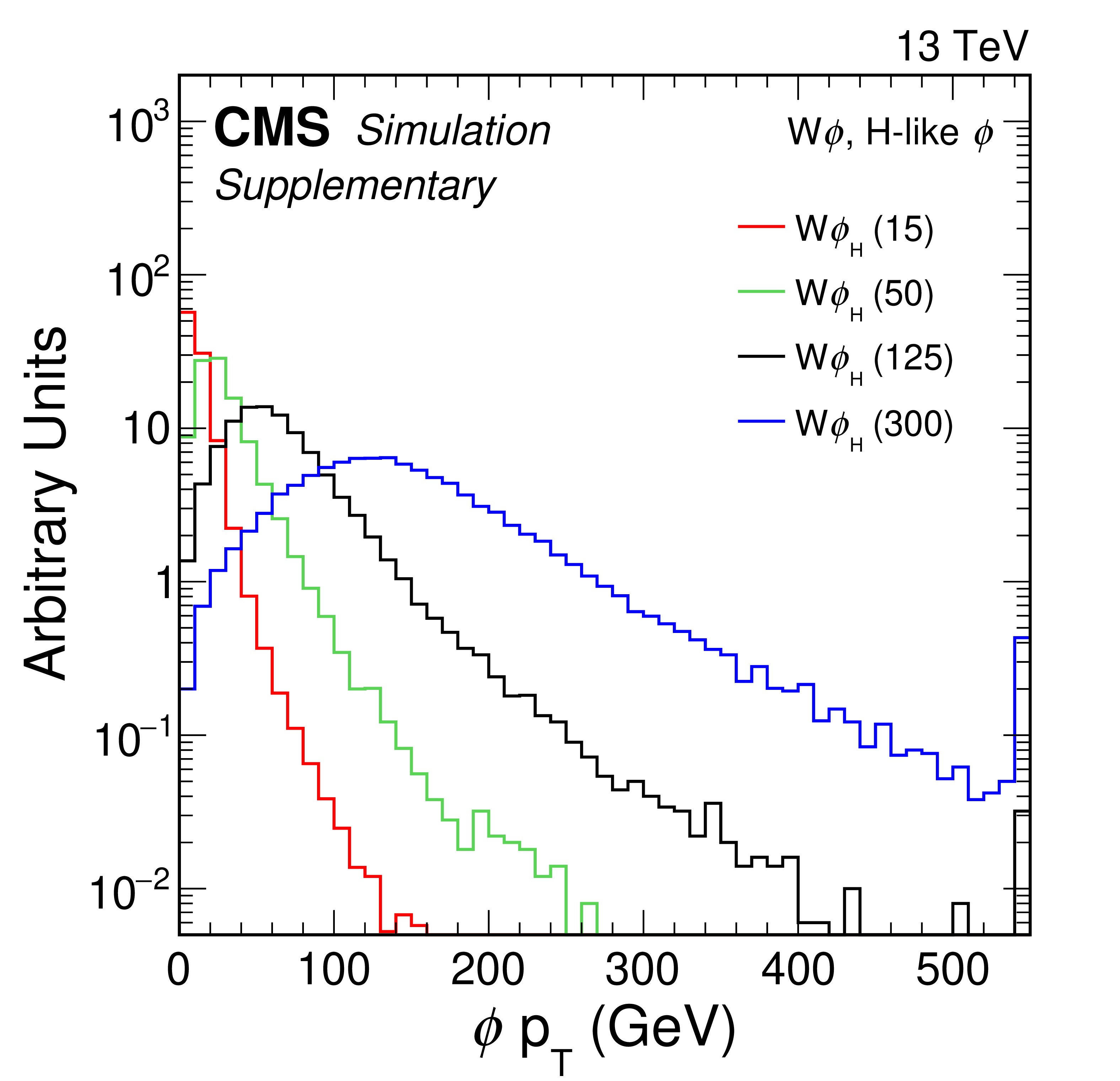
png pdf	Additional Figure 72: Generator level transverse momentum, $ p_{\mathrm{T}} $, of the $ \phi $ boson in the $ {\mathrm{W}}{\phi} $ signal with H-like couplings. Histograms are provided for several $ \phi $ masses as indicated in units of GeV, and are normalized to the same integral value. The rightmost bin contains the overflow events in each distribution.
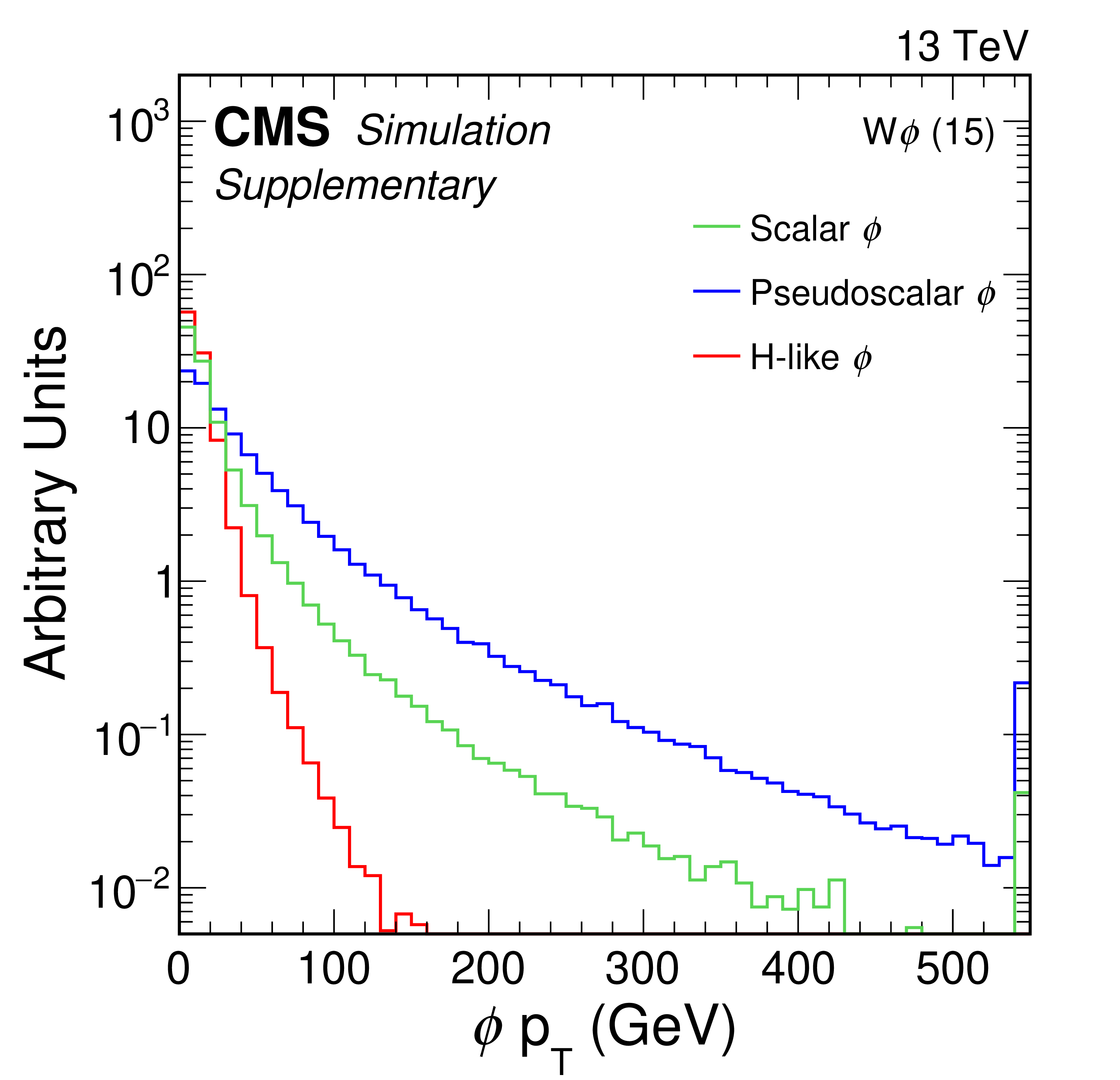
png pdf	Additional Figure 73: Generator level transverse momentum, $ p_{\mathrm{T}} $, of the $ \phi $ boson with a mass of 15 GeV in the $ {\mathrm{W}}{\phi} $ signal. Histograms are provided for scalar, pseudoscalar, and H-like $ \phi $ coupling scenarios, and are normalized to the same integral value. The rightmost bin contains the overflow events in each distribution.
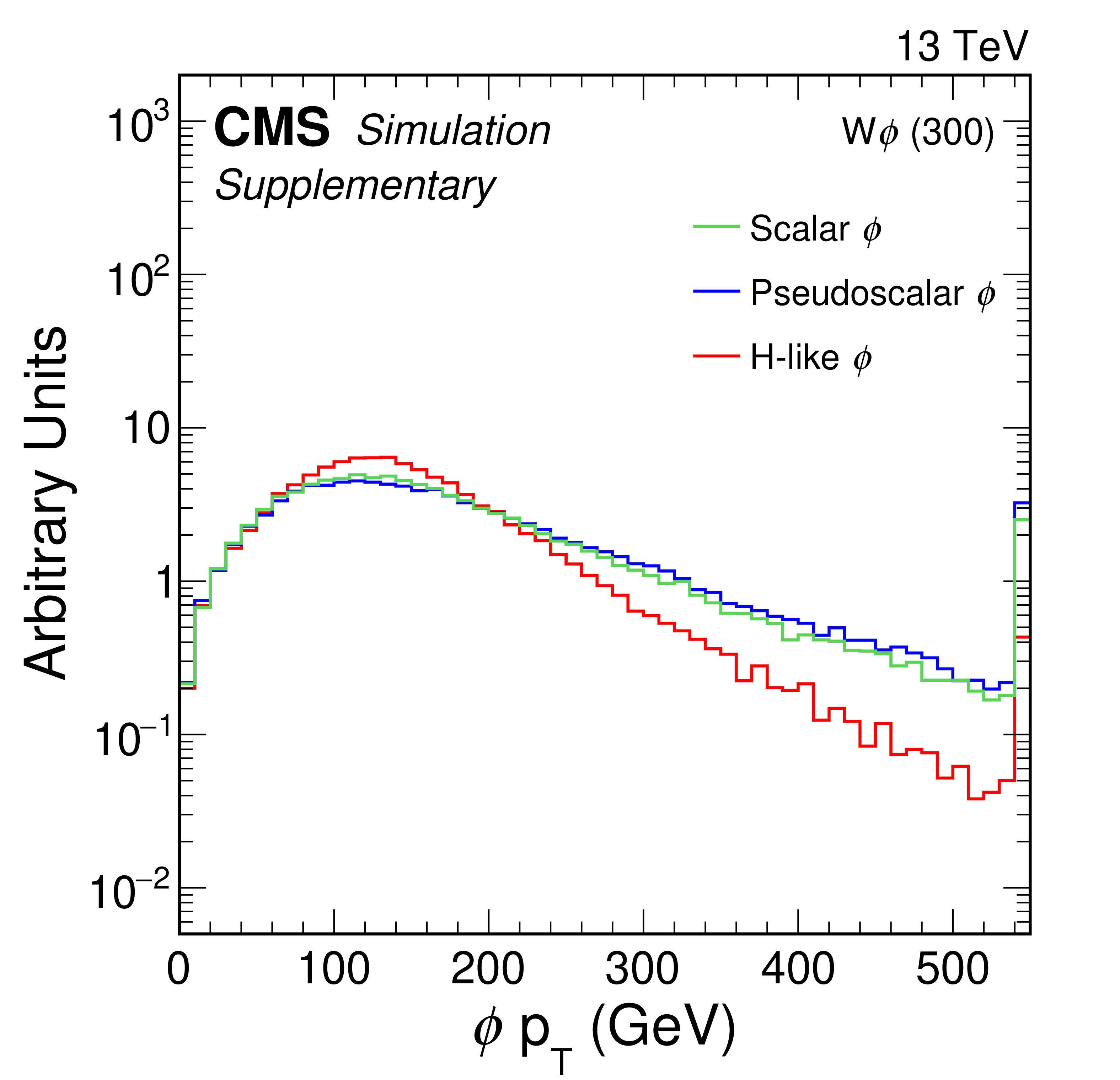
png pdf	Additional Figure 74: Generator level transverse momentum, $ p_{\mathrm{T}} $, of the $ \phi $ boson with a mass of 300 GeV in the $ {\mathrm{W}}{\phi} $ signal. Histograms are provided for scalar, pseudoscalar, and H-like $ \phi $ coupling scenarios, and are normalized to the same integral value. The rightmost bin contains the overflow events in each distribution.
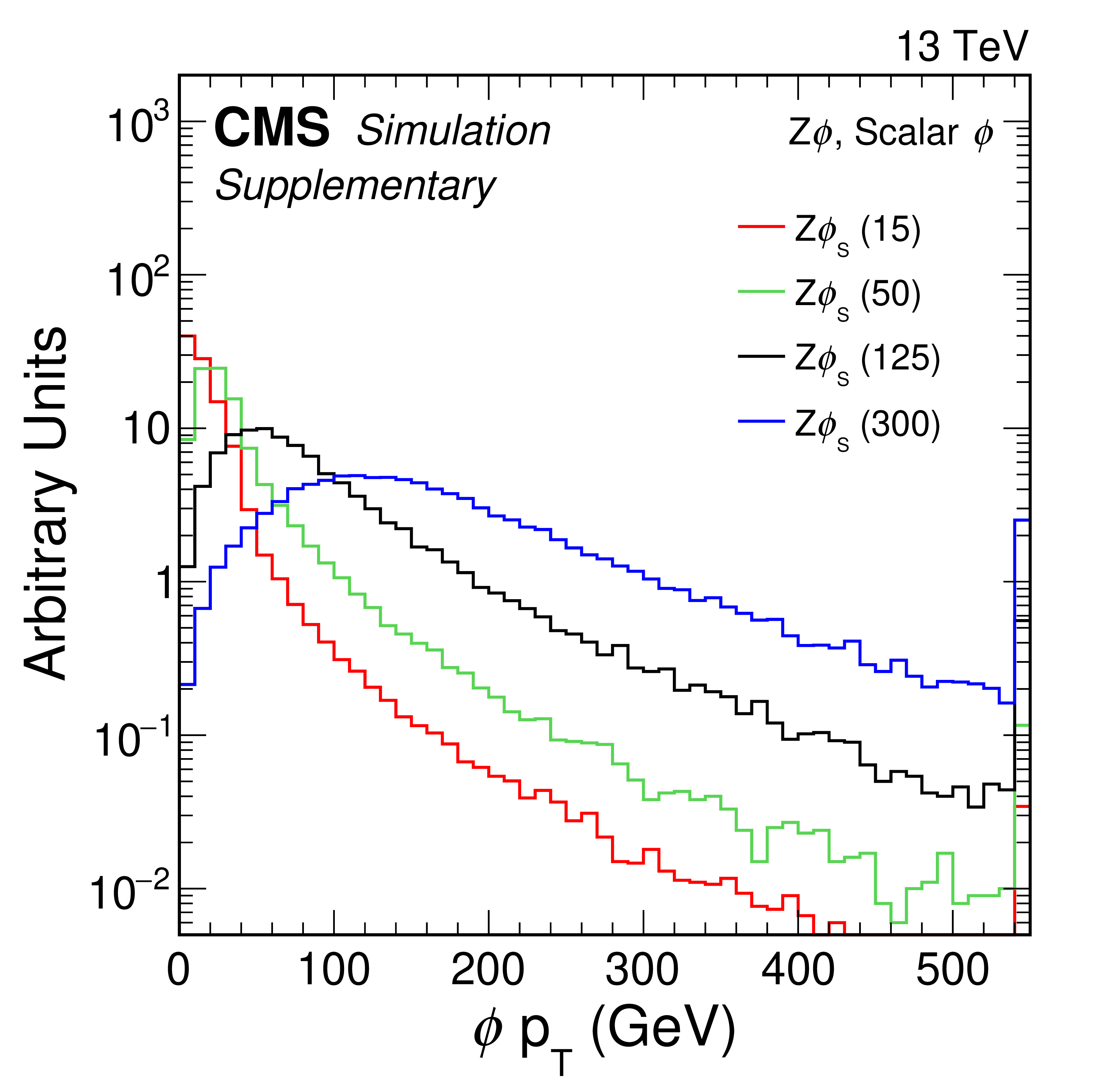
png pdf	Additional Figure 75: Generator level transverse momentum, $ p_{\mathrm{T}} $, of the $ \phi $ boson in the $ {\mathrm{Z}}{\phi} $ signal with scalar couplings. Histograms are provided for several $ \phi $ masses as indicated in units of GeV, and are normalized to the same integral value. The rightmost bin contains the overflow events in each distribution.
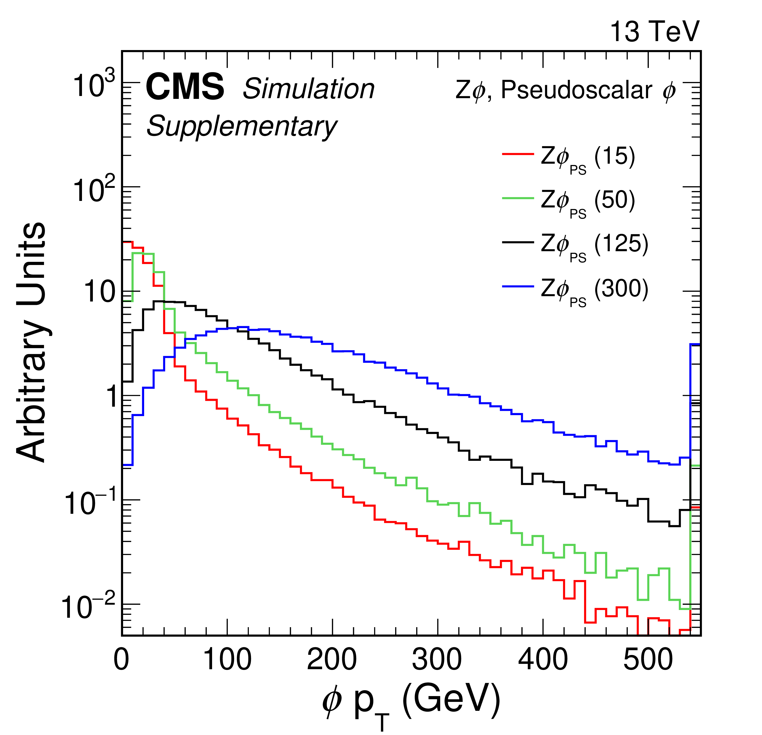
png pdf	Additional Figure 76: Generator level transverse momentum, $ p_{\mathrm{T}} $, of the $ \phi $ boson in the $ {\mathrm{Z}}{\phi} $ signal with pseudoscalar couplings. Histograms are provided for several $ \phi $ masses as indicated in units of GeV, and are normalized to the same integral value. The rightmost bin contains the overflow events in each distribution.
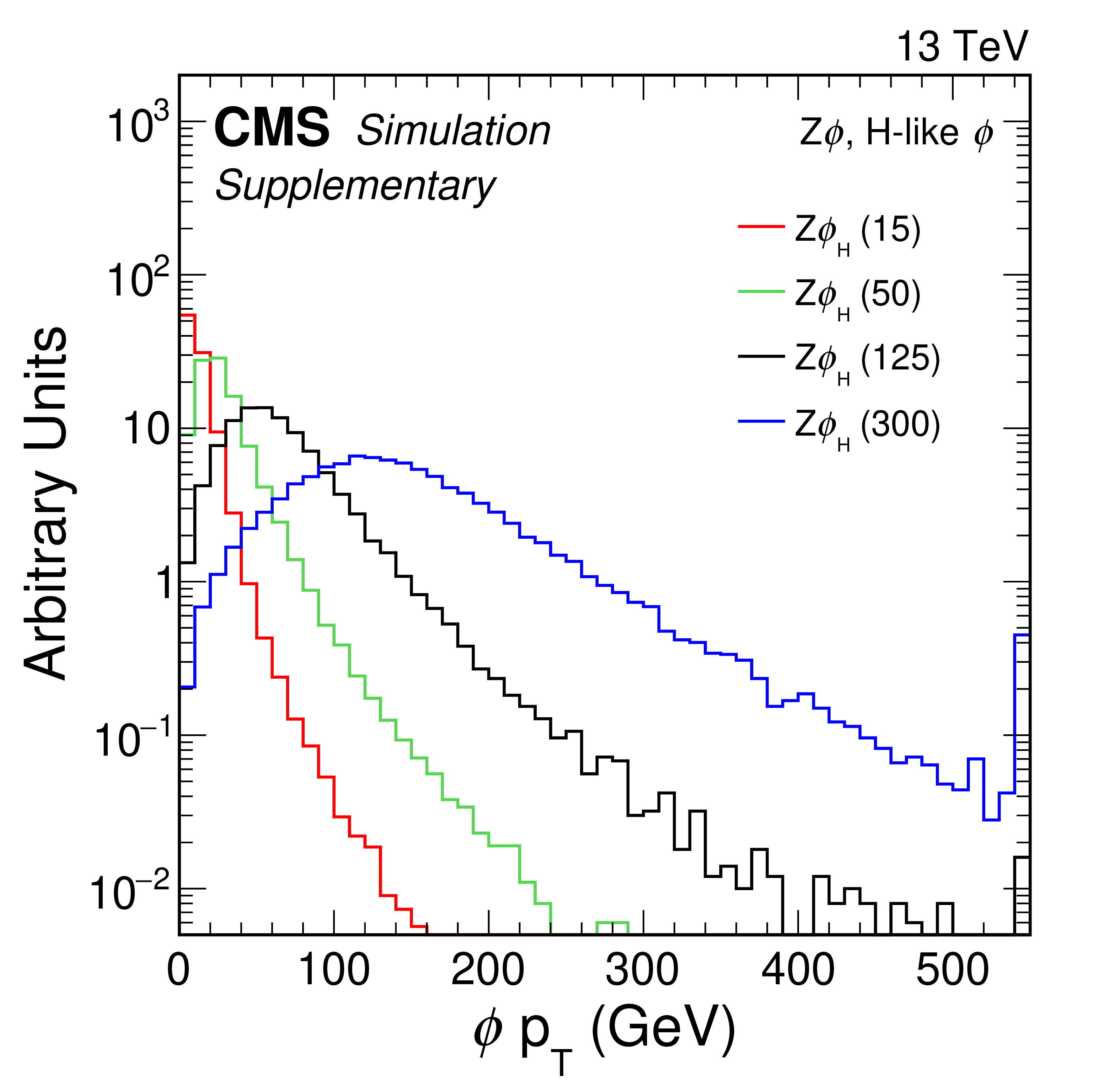
png pdf	Additional Figure 77: Generator level transverse momentum, $ p_{\mathrm{T}} $, of the $ \phi $ boson in the $ {\mathrm{Z}}{\phi} $ signal with H-like production. Histograms are provided for several $ \phi $ masses as indicated in units of GeV, and are normalized to the same integral value. The rightmost bin contains the overflow events in each distribution.
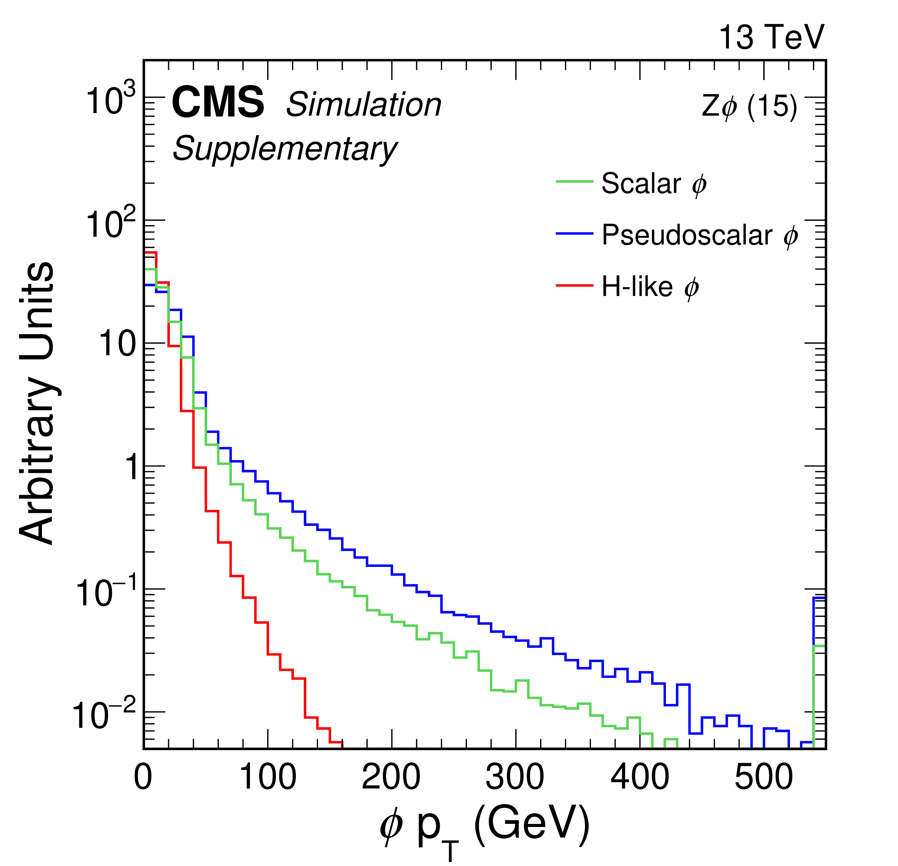
png pdf	Additional Figure 78: Generator level transverse momentum, $ p_{\mathrm{T}} $, of the $ \phi $ boson with mass of 15 GeV in the $ {\mathrm{Z}}{\phi} $ signal. Histograms are provided for scalar, pseudoscalar, and H-like $ \phi $ coupling scenarios, and are normalized to the same integral value. The rightmost bin contains the overflow events in each distribution.
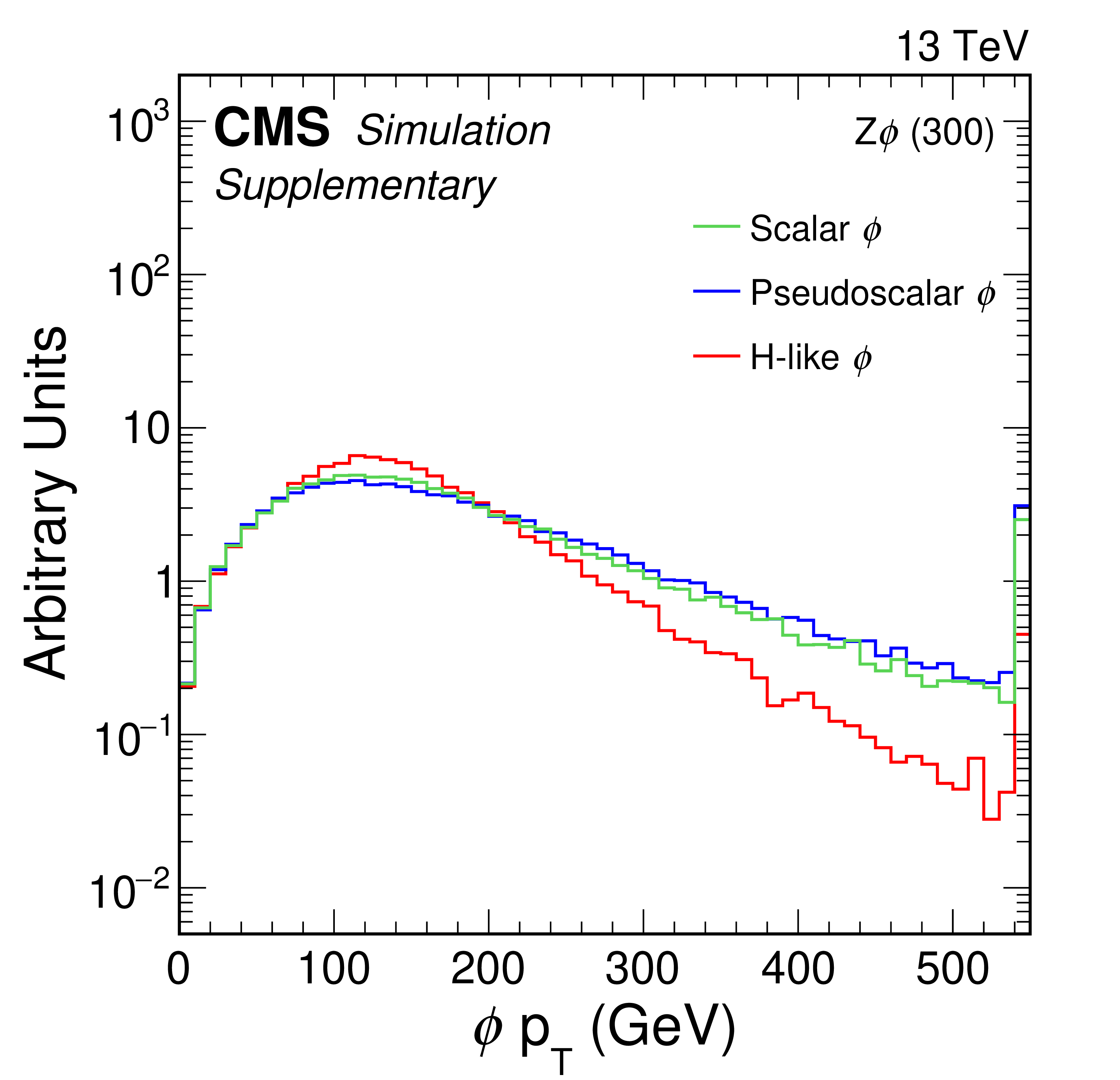
png pdf	Additional Figure 79: Generator level transverse momentum, $ p_{\mathrm{T}} $, of the $ \phi $ boson with mass of 300 GeV in the $ {\mathrm{Z}}{\phi} $ signal. Histograms are provided for scalar, pseudoscalar, and\ H-like $ \phi $ coupling scenarios, and are normalized to the same integral value. The rightmost bin contains the overflow events in each distribution.
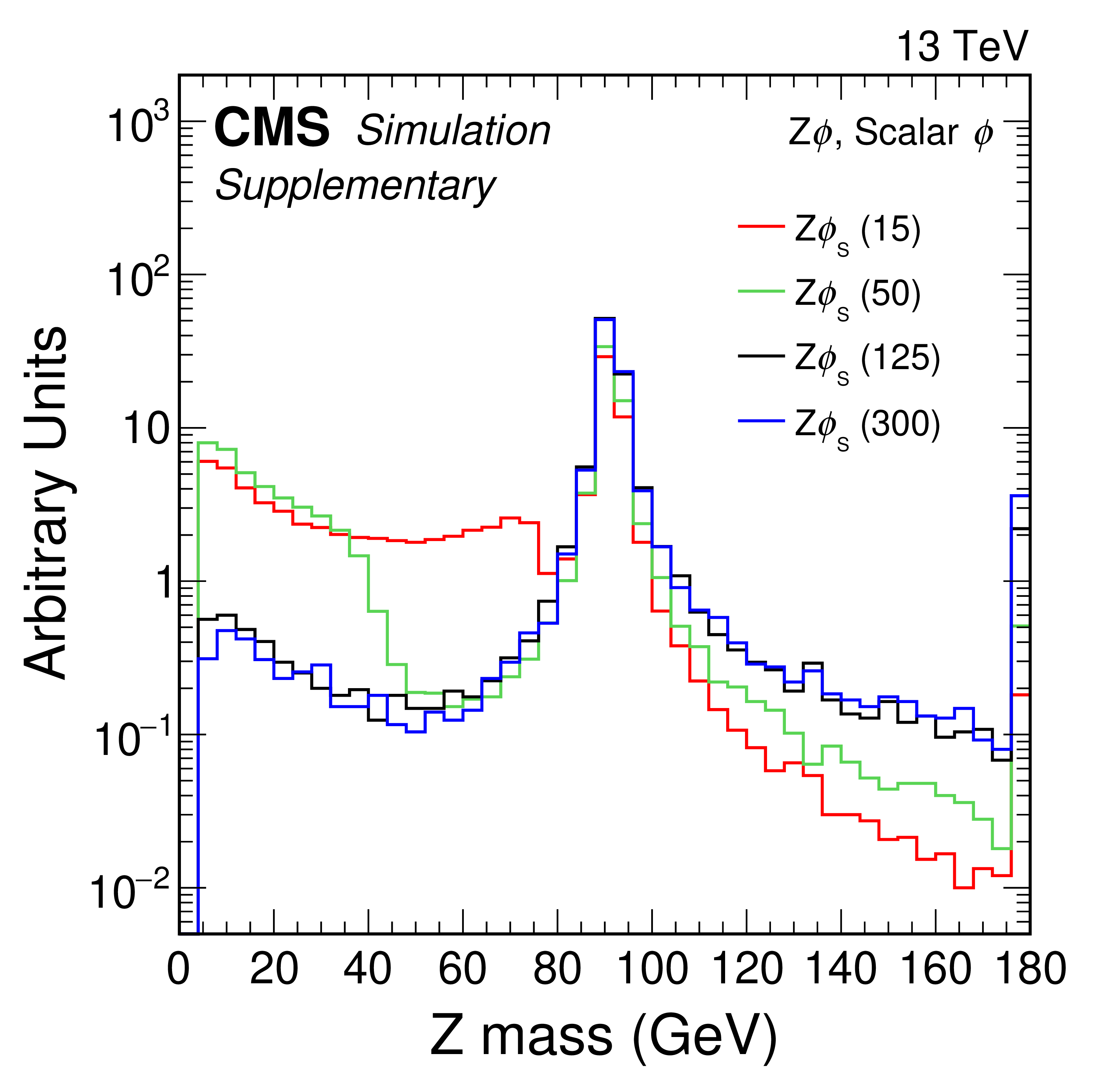
png pdf	Additional Figure 80: Generator level Z boson reconstructed mass in the $ {\mathrm{Z}}{\phi} $ signal with scalar couplings. Histograms are provided for several $ \phi $ masses as indicated in units of GeV, and are normalized to the same integral value. The rightmost bin contains the overflow events in each distribution.
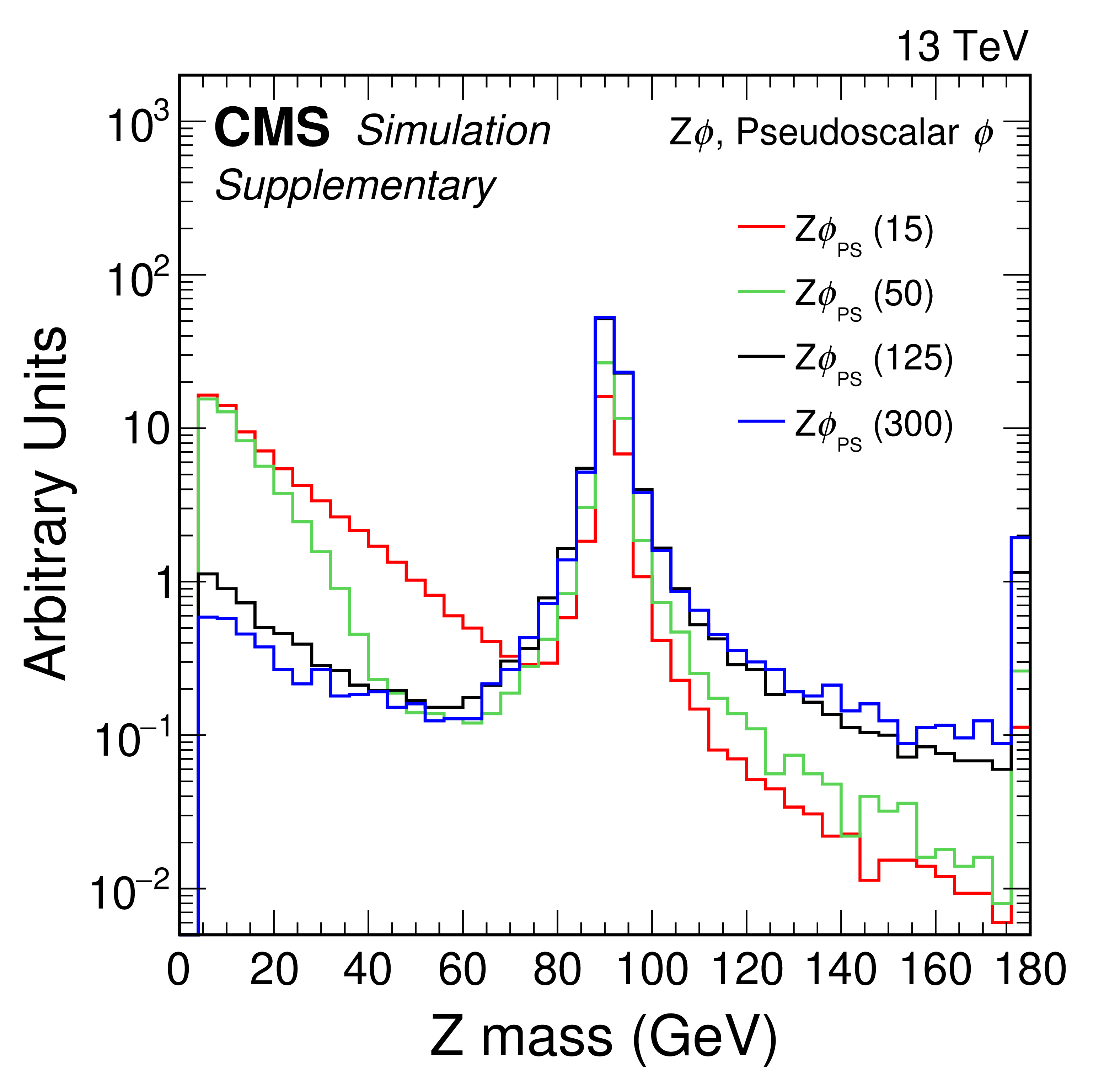
png pdf	Additional Figure 81: Generator level Z boson reconstructed mass in the $ {\mathrm{Z}}{\phi} $ signal with pseudoscalar couplings. Histograms are provided for several $ \phi $ masses as indicated in units of GeV, and are normalized to the same integral value. The rightmost bin contains the overflow events in each distribution.
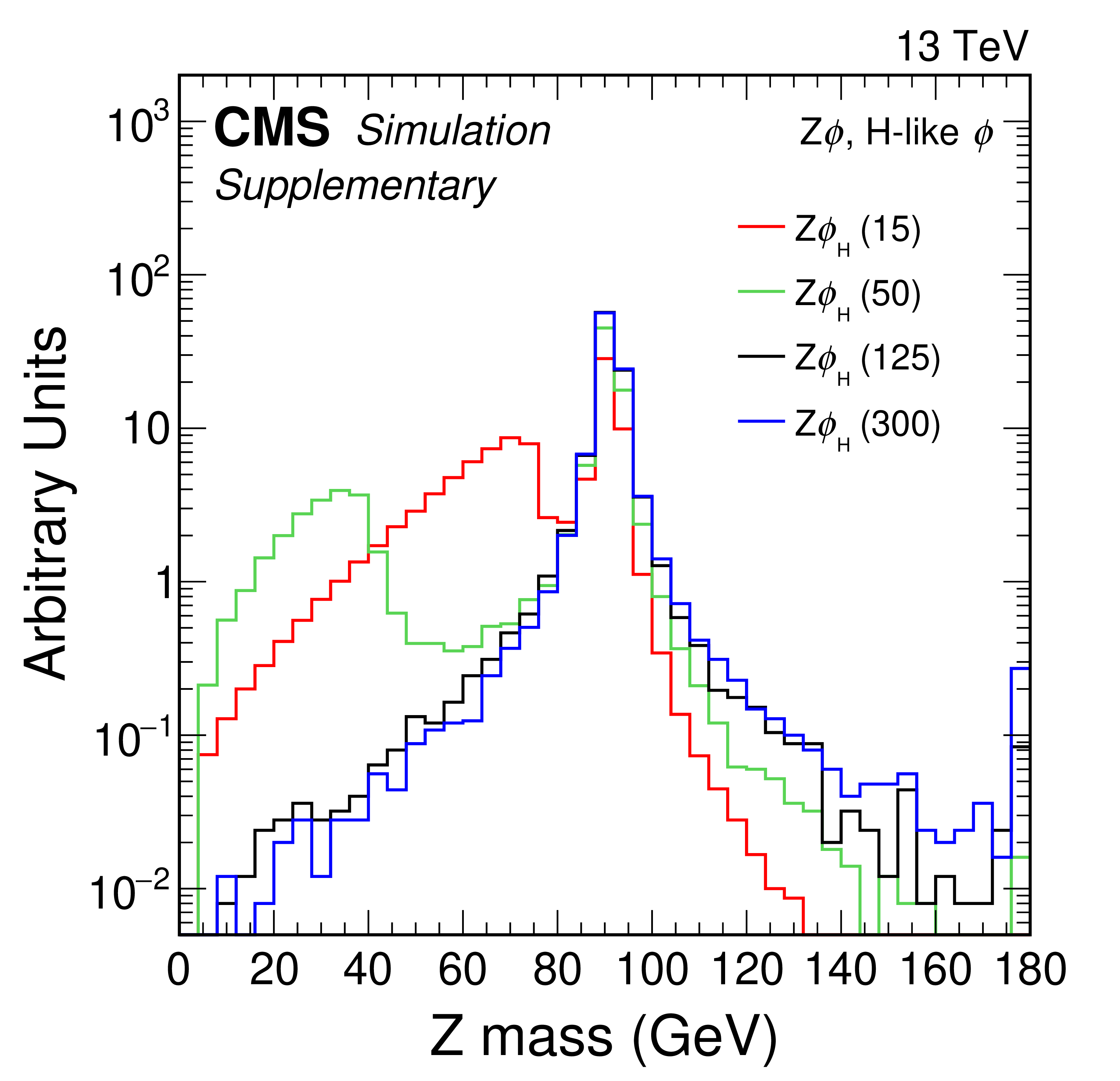
png pdf	Additional Figure 82: Generator level Z boson reconstructed mass in the $ {\mathrm{Z}}{\phi} $ signal with H-like production. Histograms are provided for several $ \phi $ masses as indicated in units of GeV, and are normalized to the same integral value. The rightmost bin contains the overflow events in each distribution.
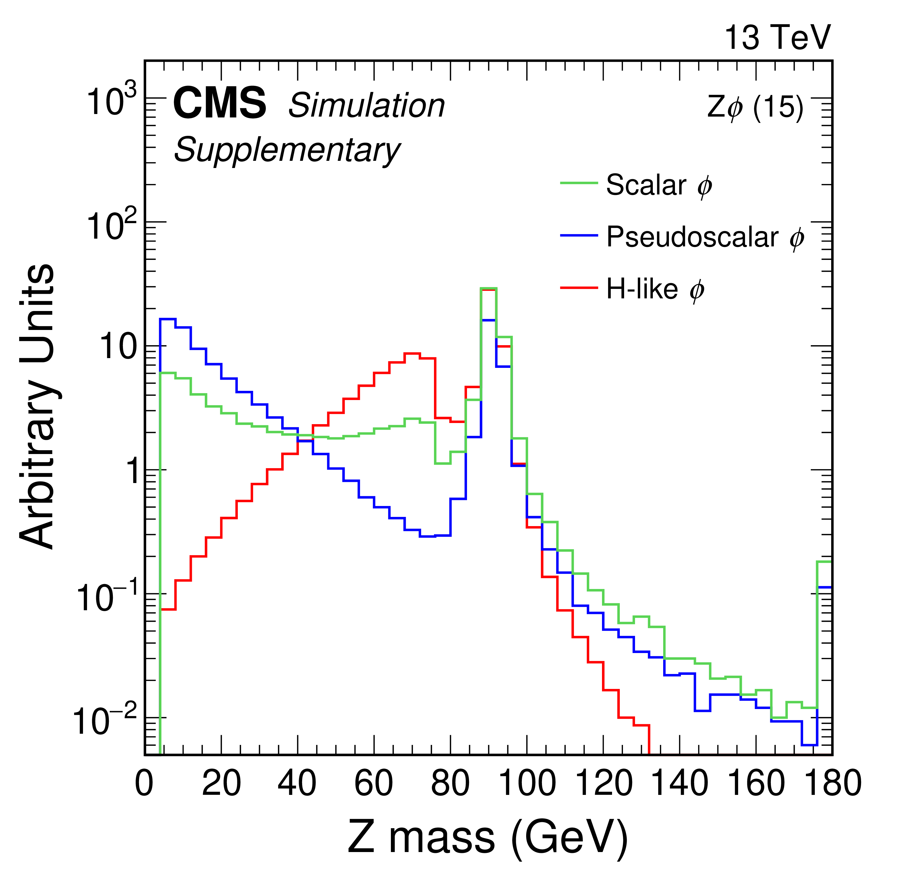
png pdf	Additional Figure 83: Generator level Z boson reconstructed mass in the $ {\mathrm{Z}}{\phi} $ signal with a $ \phi $ boson mass of 15 GeV. Histograms are provided for scalar, pseudoscalar, and H-like $ \phi $ coupling scenarios, and are normalized to the same integral value. The rightmost bin contains the overflow events in each distribution.
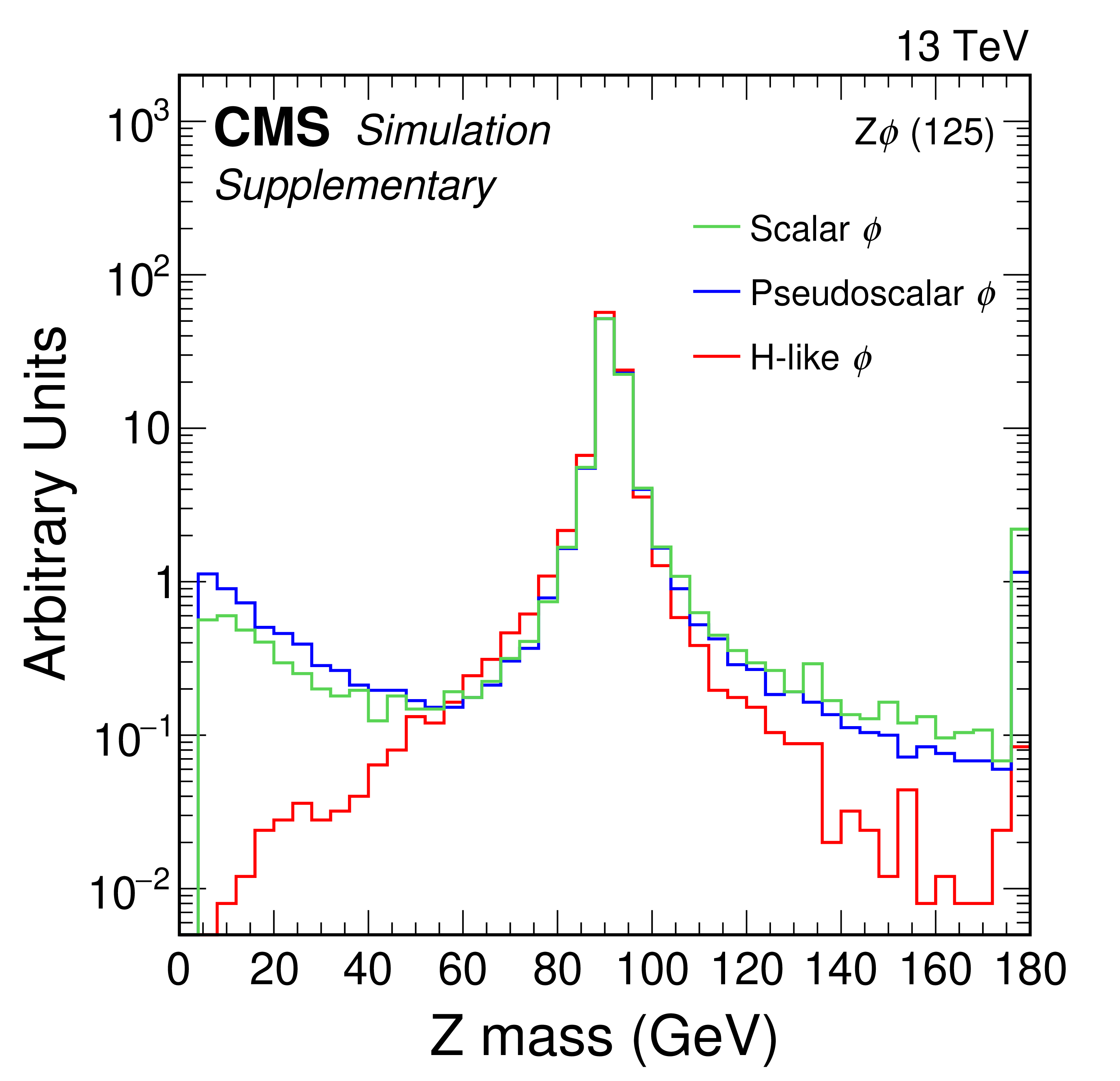
png pdf	Additional Figure 84: Generator level Z boson reconstructed mass in the $ {\mathrm{Z}}{\phi} $ signal with a $ \phi $ boson mass of 125 GeV. Histograms are provided for scalar, pseudoscalar, and H-like $ \phi $ coupling scenarios, and are normalized to the same integral value. The rightmost bin contains the overflow events in each distribution.
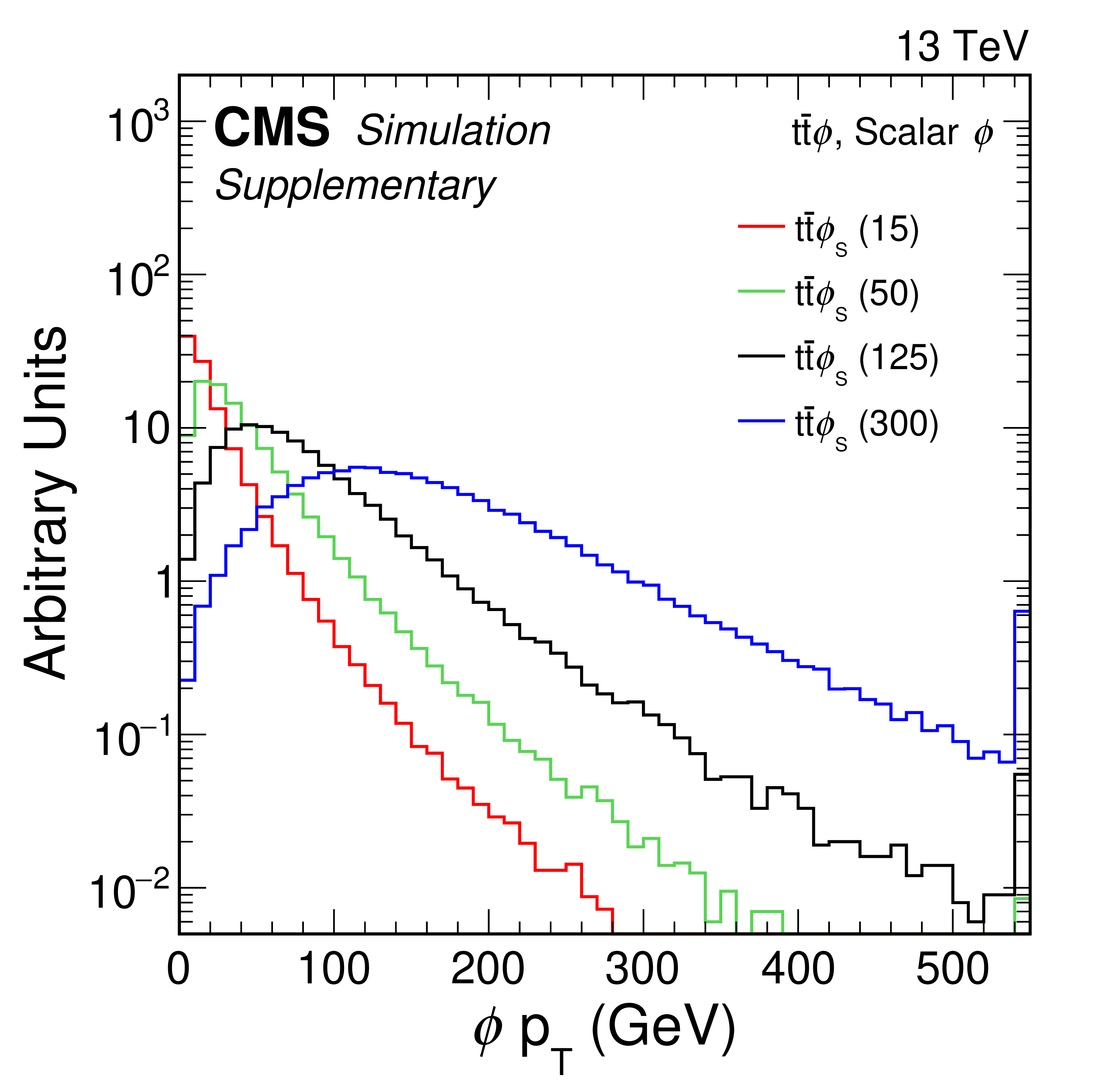
png pdf	Additional Figure 85: Generator level transverse momentum, $ p_{\mathrm{T}} $, of $ \phi $ boson in the $ {{\mathrm{t}\overline{\mathrm{t}}} }{\phi} $ signal with scalar couplings. Histograms are provided for several $ \phi $ masses as indicated in units of GeV, and are normalized to the same integral value. The rightmost bin contains the overflow events in each distribution.
png pdf	Additional Figure 86: Generator level transverse momentum, $ p_{\mathrm{T}} $, of the $ \phi $ boson in the $ {{\mathrm{t}\overline{\mathrm{t}}} }{\phi} $ signal with pseudoscalar couplings. Histograms are provided for several $ \phi $ masses as indicated in units of GeV, and are normalized to the same integral value. The rightmost bin contains the overflow events in each distribution.
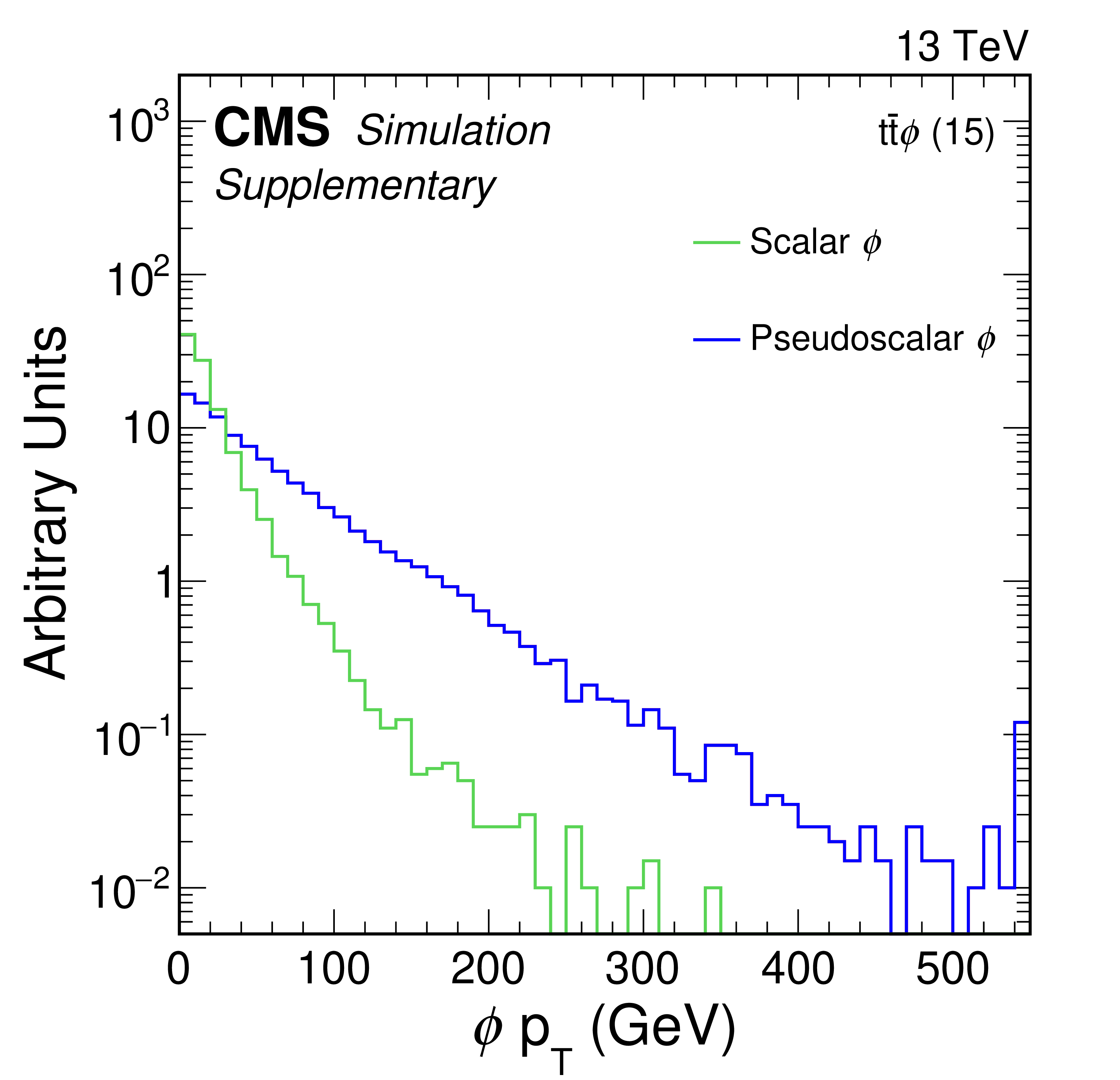
png pdf	Additional Figure 87: Generator level transverse momentum, $ p_{\mathrm{T}} $, of $ \phi $ boson with mass of 15 GeV in the $ {{\mathrm{t}\overline{\mathrm{t}}} }{\phi} $ signal. Histograms are provided for scalar and pseudoscalar $ \phi $ coupling scenarios, and are normalized to the same integral value. The rightmost bin contains the overflow events in each distribution.
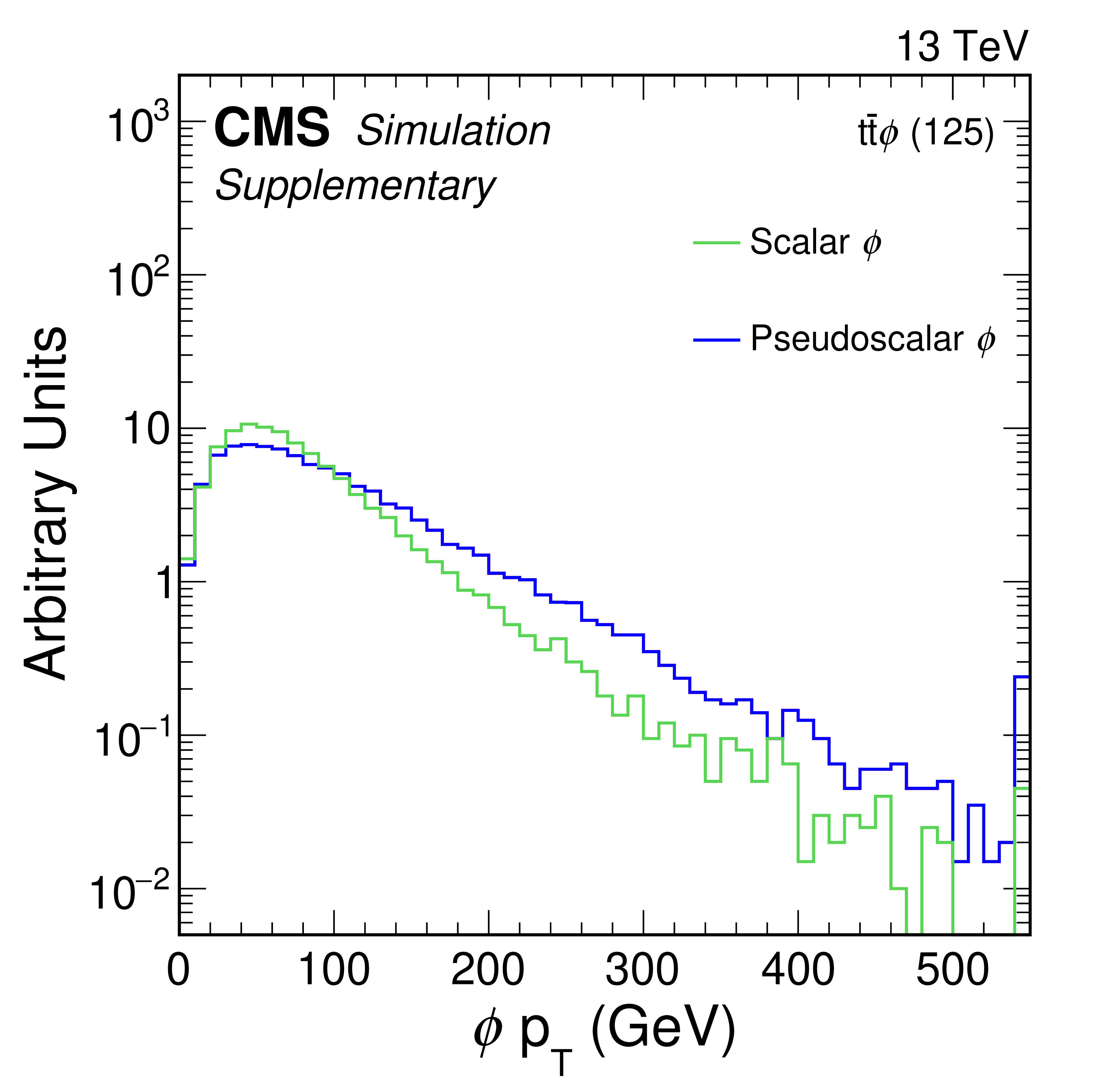
png pdf	Additional Figure 88: Generator level transverse momentum, $ p_{\mathrm{T}} $, of $ \phi $ boson with mass of 125 GeV in the $ {{\mathrm{t}\overline{\mathrm{t}}} }{\phi} $ signal. Histograms are provided for scalar and pseudoscalar $ \phi $ coupling scenarios, and are normalized to the same integral value. The rightmost bin contains the overflow events in each distribution.
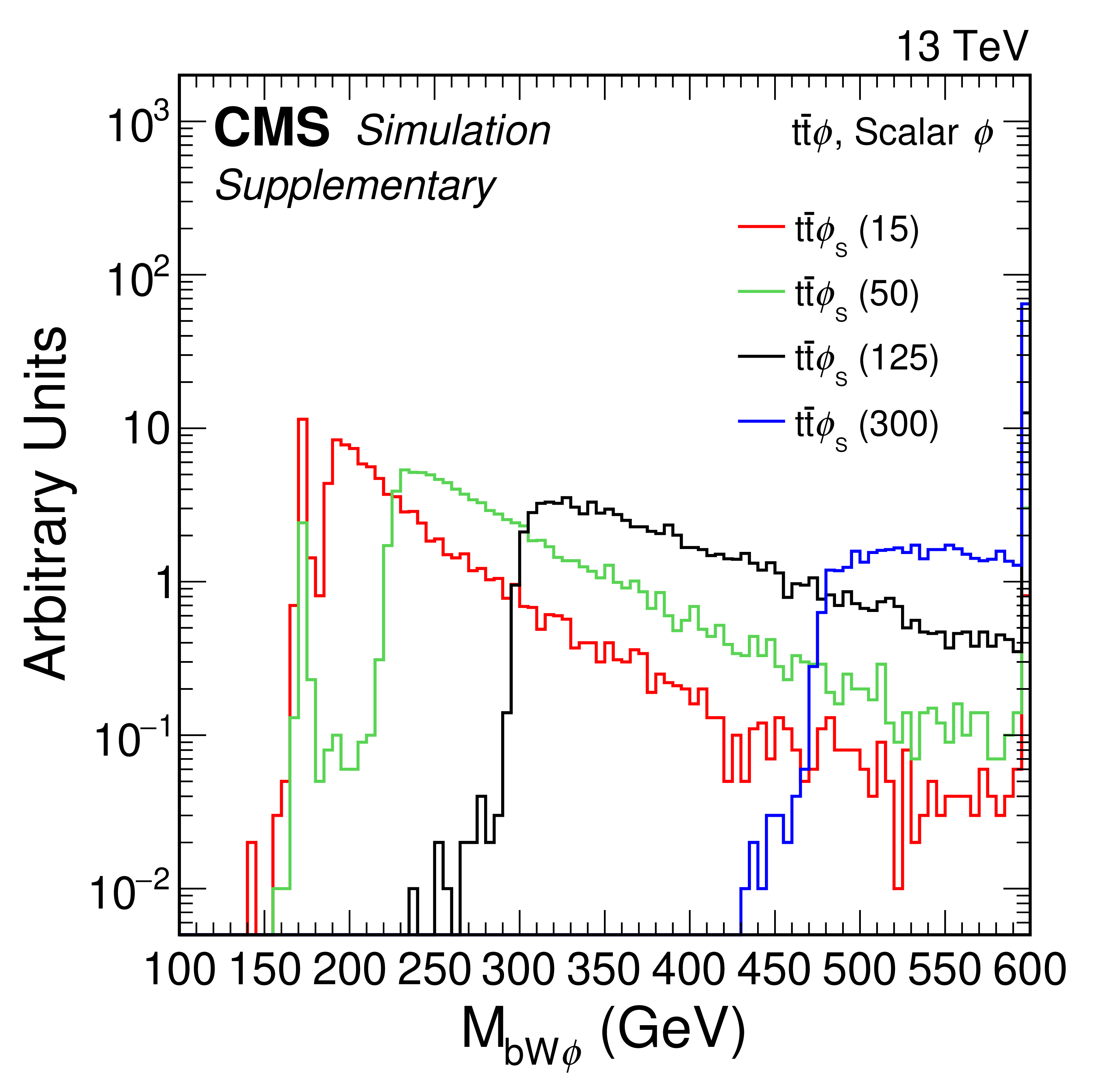
png pdf	Additional Figure 89: Generator level invariant mass of the b quark, W boson, and $ \phi $ boson three-body system in the $ {{\mathrm{t}\overline{\mathrm{t}}} }{\phi} $ signal with scalar coupling. Histograms are provided for several $ \phi $ masses as indicated in units of GeV, and are normalized to the same integral value. The rightmost bin contains the overflow events in each distribution.
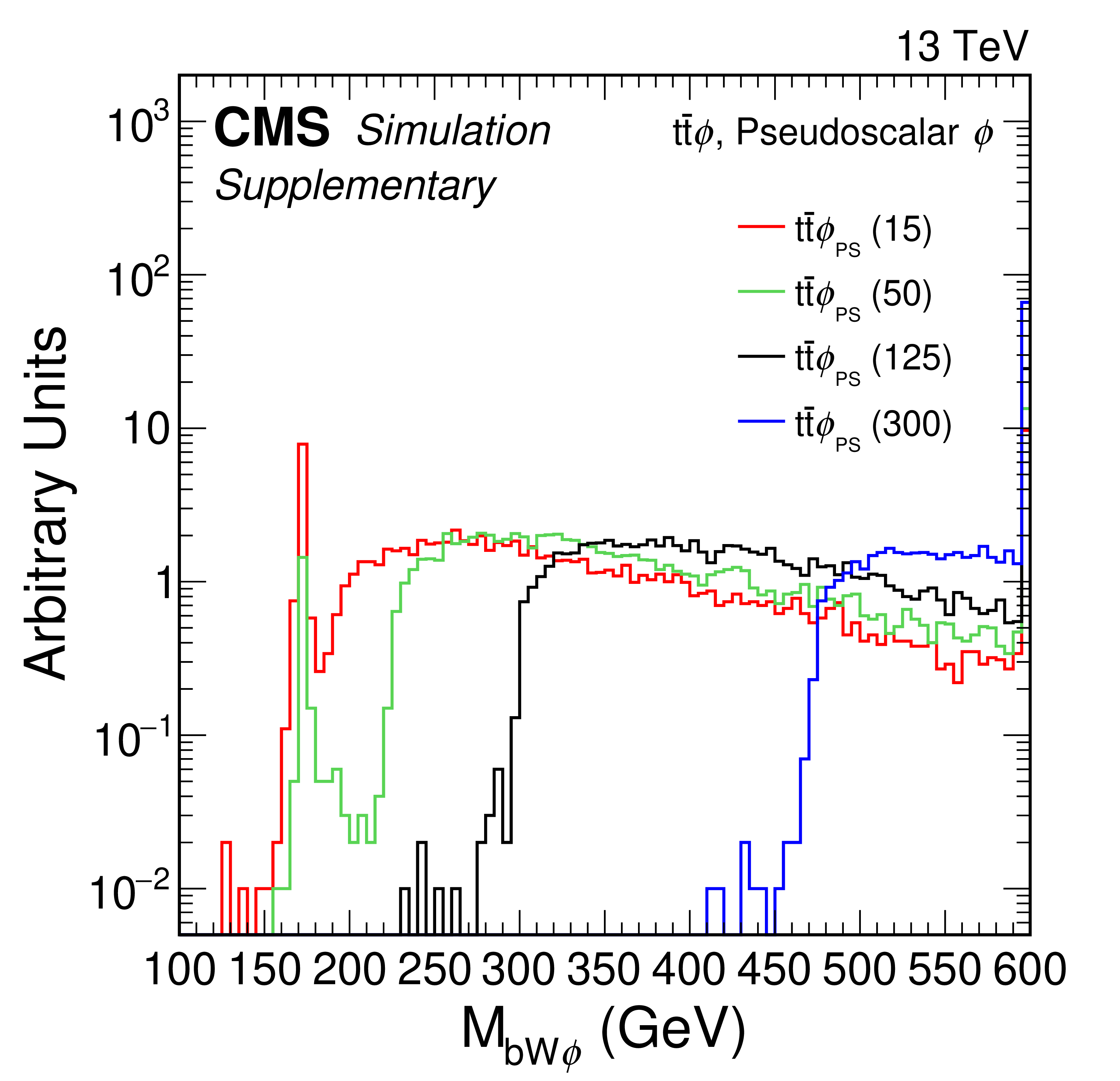
png pdf	Additional Figure 90: Generator level invariant mass of the b quark, W boson, and $ \phi $ boson three-body system in the $ {{\mathrm{t}\overline{\mathrm{t}}} }{\phi} $ signal with pseudoscalar coupling. Histograms are provided for several $ \phi $ masses as indicated in units of GeV, and are normalized to the same integral value. The rightmost bin contains the overflow events in each distribution.
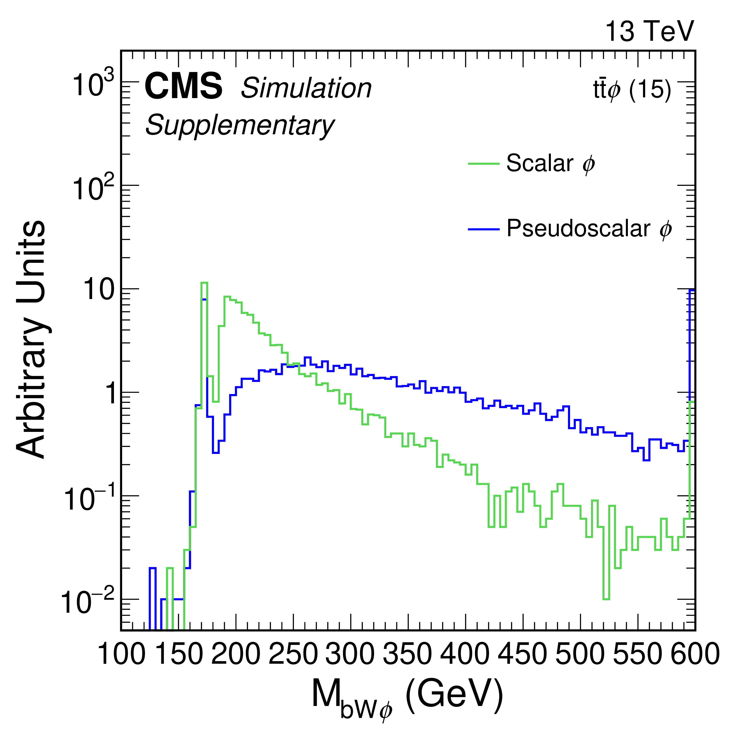
png pdf	Additional Figure 91: Generator level invariant mass of the b quark, W boson, and $ \phi $ boson three-body system with $ \phi $ mass of 15 GeV in the $ {{\mathrm{t}\overline{\mathrm{t}}} }{\phi} $ signal. Histograms are provided for scalar and pseudoscalar $ \phi $ coupling scenarios, and are normalized to the same integral value. The rightmost bin contains the overflow events in each distribution.
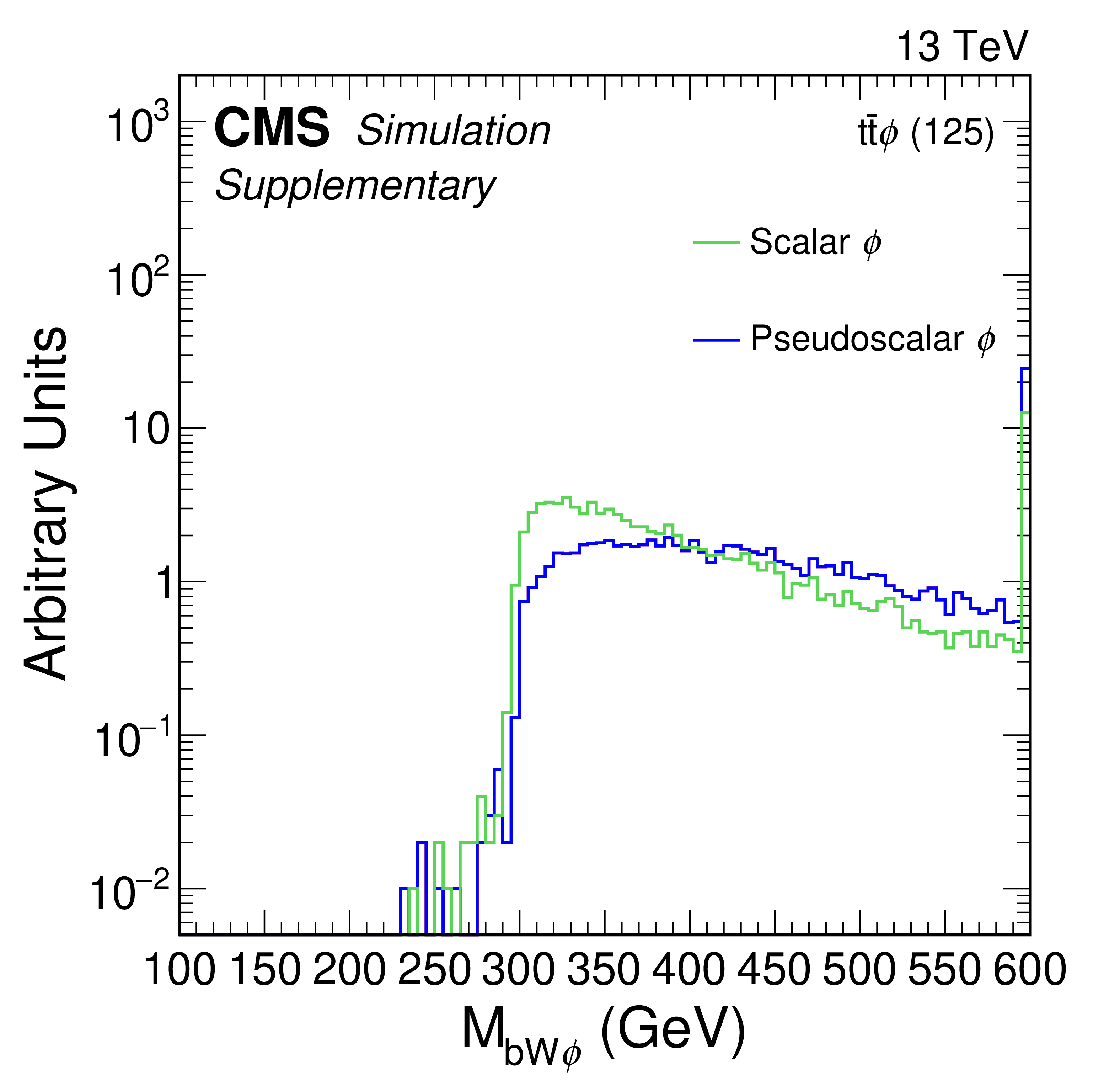
png pdf	Additional Figure 92: Generator level invariant mass of the b quark, W boson, and $ \phi $ boson three-body system with $ \phi $ mass of 125 GeV in the $ {{\mathrm{t}\overline{\mathrm{t}}} }{\phi} $ signal. Histograms are provided for scalar and pseudoscalar $ \phi $ coupling scenarios, and are normalized to the same integral value. The rightmost bin contains the overflow events in each distribution.

References
1	G. Cacciapaglia, G. Ferretti, T. Flacke, and H. Serodio	Light scalars in composite Higgs models	Front. Phys. 7 (2019) 22	1902.06890
2	U. Ellwanger, C. Hugonie, and A. M. Teixeira	The next-to-minimal supersymmetric standard model	Phys. Rept. 496 (2010) 1	0910.1785
3	M. Maniatis	The next-to-minimal supersymmetric extension of the standard model reviewed	Int. J. Mod. Phys. A 25 (2010) 3505	0906.0777
4	M. R. Buckley, D. Feld, and D. Goncalves	Scalar simplified models for dark matter	PRD 91 (2015) 015017	1410.6497
5	M. Casolino et al.	Probing a light CP-odd scalar in di-top-associated production at the LHC	EPJC 75 (2015) 498	1507.07004
6	W.-F. Chang, T. Modak, and J. N. Ng	Signal for a light singlet scalar at the LHC	PRD 97 (2018) 055020	1711.05722
7	P. Artoisenet et al.	A framework for Higgs characterisation	JHEP 11 (2013) 043	1306.6464
8	T. Ghosh, H.-K. Guo, T. Han, and H. Liu	Electroweak phase transition with an SU(2) dark sector	JHEP 07 (2021) 045	2012.09758
9	E. Gildener and S. Weinberg	Symmetry breaking and scalar bosons	PRD 13 (1976) 3333
10	W. D. Goldberger, B. Grinstein, and W. Skiba	Distinguishing the Higgs boson from the dilaton at the Large Hadron Collider	PRL 100 (2008) 111802	0708.1463
11	A. Ahmed, A. Mariotti, and S. Najjari	A light dilaton at the LHC	JHEP 05 (2020) 093	1912.06645
12	V. Barger, M. Ishida, and W.-Y. Keung	Dilaton at the LHC	PRD 85 (2012) 015024	1111.2580
13	H. Georgi, D. B. Kaplan, and L. Randall	Manifesting the invisible axion at low-energies	PLB 169 (1986) 73
14	K. Mimasu and V. Sanz	ALPs at colliders	JHEP 06 (2015) 173	1409.4792
15	I. Brivio et al.	ALPs effective field theory and collider signatures	EPJC 77 (2017) 572	1701.05379
16	M. Bauer, M. Heiles, M. Neubert, and A. Thamm	Axion-like particles at future colliders	EPJC 79 (2019) 74	1808.10323
17	R. M. Schabinger and J. D. Wells	A minimal spontaneously broken hidden sector and its impact on Higgs boson physics at the large hadron collider	PRD 72 (2005) 093007	hep-ph/0509209
18	V. Barger et al.	LHC phenomenology of an extended standard model with a real scalar singlet	PRD 77 (2008) 035005	0706.4311
19	CMS Collaboration	HEPData record for this analysis	link
20	ALEPH Collaboration	Search for a nonminimal Higgs boson produced in the reaction $ \mathrm{e}^{+} \mathrm{e}^{-} \to \mathrm{h}\mathrm{Z}^{*} $	PLB 313 (1993) 312
21	L3 Collaboration	Search for neutral Higgs boson production through the process $ \mathrm{e}^{+} \mathrm{e}^{-} \to \mathrm{Z}^{*}\mathrm{H}^0 $	PLB 385 (1996) 454
22	LEP working group for Higgs boson searches, ALEPH, DELPHI, L3 and OPAL Collaborations	Search for the standard model Higgs boson at LEP	PLB 565 (2003) 61	hep-ex/0306033
23	D0 Collaboration	Combined search for the Higgs boson with the D0 experiment	PRD 88 (2013) 052011	1303.0823
24	CDF Collaboration	Combination of searches for the Higgs boson using the full CDF data set	PRD 88 (2013) 052013	1301.6668
25	CDF and D0 Collaborations	Higgs boson studies at the Tevatron	PRD 88 (2013) 052014	1303.6346
26	CMS Collaboration	Search for the standard model Higgs boson produced in association with W and Z bosons in pp collisions at $ \sqrt{s}= $ 7 TeV	JHEP 11 (2012) 088	CMS-HIG-12-010 1209.3937
27	ATLAS Collaboration	Measurement of the production cross section for a Higgs boson in association with a vector boson in the $ \mathrm{H} \to \mathrm{WW}^{\ast} \to \ell\nu\ell\nu $ channel in pp collisions at $ \sqrt{s}= $ 13 TeV with the ATLAS detector	PLB 798 (2019) 134949	1903.10052
28	CMS Collaboration	Evidence for the 125 GeV Higgs boson decaying to a pair of $ \tau $ leptons	JHEP 05 (2014) 104	CMS-HIG-13-004 1401.5041
29	ATLAS Collaboration	Evidence for the Higgs-boson Yukawa coupling to tau leptons with the ATLAS detector	JHEP 04 (2015) 117	1501.04943
30	CMS Collaboration	Search for the associated production of the Higgs boson with a top-quark pair	[Erratum: JHEP 10, 106 ()], 2014 JHEP 09 (2014) 087	CMS-HIG-13-029 1408.1682
31	ATLAS Collaboration	Search for new phenomena in events with same-charge leptons and b jets in pp collisions at $ \sqrt{s}= $ 13 TeV with the ATLAS detector	JHEP 12 (2018) 039	1807.11883
32	CMS Collaboration	Evidence for Higgs boson decay to a pair of muons	JHEP 01 (2021) 148	CMS-HIG-19-006 2009.04363
33	ATLAS Collaboration	A search for the dimuon decay of the standard model Higgs boson with the ATLAS detector	PLB 812 (2021) 135980	2007.07830
34	CMS Collaboration	Observation of Higgs boson decay to bottom quarks	PRL 121 (2018) 121801	CMS-HIG-18-016 1808.08242
35	ATLAS Collaboration	Observation of $ \mathrm{H} \to \mathrm{b}\bar{\mathrm{b}} $ decays and VH production with the ATLAS detector	PLB 786 (2018) 59	1808.08238
36	ATLAS Collaboration	Search for a new pseudoscalar decaying into a pair of muons in events with a top-quark pair at $ \sqrt{s} = $ 13 tev with the ATLAS detector	no.~9, 09, 2023 PRD 108 (2023)	2304.14247
37	CMS Collaboration	Search for physics beyond the standard model in multilepton final states in proton-proton collisions at $ \sqrt{s} = $ 13 TeV	JHEP 03 (2020) 051	CMS-EXO-19-002 1911.04968
38	CMS Collaboration	The CMS experiment at the CERN LHC	JINST 3 (2008) S08004
39	CMS Collaboration	Development of the CMS detector for the CERN LHC Run 3	Accepted by JINST, 2023	CMS-PRF-21-001 2309.05466
40	CMS Collaboration	Performance of the CMS level-1 trigger in proton-proton collisions at $ \sqrt{s} = $ 13 TeV	JINST 15 (2020) P10017	CMS-TRG-17-001 2006.10165
41	CMS Collaboration	The CMS trigger system	JINST 12 (2017) P01020	CMS-TRG-12-001 1609.02366
42	CMS Collaboration	Precision luminosity measurement in proton-proton collisions at $ \sqrt{s} = $ 13 TeV in 2015 and 2016 at CMS	EPJC 81 (2021) 800	CMS-LUM-17-003 2104.01927
43	CMS Collaboration	CMS luminosity measurement for the 2017 data-taking period at $ \sqrt{s} = $ 13 TeV	CMS Physics Analysis Summary, 2018 CMS-PAS-LUM-17-004	CMS-PAS-LUM-17-004
44	CMS Collaboration	CMS luminosity measurement for the 2018 data-taking period at $ \sqrt{s} = $ 13 TeV	CMS Physics Analysis Summary, 2019 CMS-PAS-LUM-18-002	CMS-PAS-LUM-18-002
45	J. Alwall et al.	The automated computation of tree-level and next-to-leading order differential cross sections, and their matching to parton shower simulations	JHEP 07 (2014) 079	1405.0301
46	P. Nason	A new method for combining NLO QCD with shower Monte Carlo algorithms	JHEP 11 (2004) 040	hep-ph/0409146
47	S. Frixione, P. Nason, and C. Oleari	Matching NLO QCD computations with parton shower simulations: the POWHEG method	JHEP 11 (2007) 070	0709.2092
48	S. Alioli, P. Nason, C. Oleari, and E. Re	A general framework for implementing NLO calculations in shower Monte Carlo programs: the POWHEG BOX	JHEP 06 (2010) 043	1002.2581
49	J. M. Campbell and R. K. Ellis	MCFM for the Tevatron and the LHC	--206 10, 2010 Nucl. Phys. Proc. Suppl. 20 (2010) 5	1007.3492
50	Y. Gao et al.	Spin determination of single-produced resonances at hadron colliders	PRD 81 (2010) 075022	1001.3396
51	S. Bolognesi et al.	On the spin and parity of a single-produced resonance at the LHC	PRD 86 (2012) 095031	1208.4018
52	I. Anderson et al.	Constraining anomalous HVV interactions at proton and lepton colliders	PRD 89 (2014) 035007	1309.4819
53	A. V. Gritsan, R. Röntsch, M. Schulze, and M. Xiao	Constraining anomalous Higgs boson couplings to the heavy flavor fermions using matrix element techniques	PRD 94 (2016) 055023	1606.03107
54	NNPDF Collaboration	Parton distributions for the LHC Run II	JHEP 04 (2015) 040	1410.8849
55	NNPDF Collaboration	Parton distributions from high-precision collider data	EPJC 77 (2017) 663	1706.00428
56	T. Sjöstrand et al.	An introduction to PYTHIA 8.2	Comput. Phys. Commun. 191 (2015) 159	1410.3012
57	CMS Collaboration	Event generator tunes obtained from underlying event and multiparton scattering measurements	EPJC 76 (2016) 155	CMS-GEN-14-001 1512.00815
58	CMS Collaboration	Extraction and validation of a new set of CMS PYTHIA8 tunes from underlying-event measurements	EPJC 80 (2020) 4	CMS-GEN-17-001 1903.12179
59	J. Alwall et al.	Comparative study of various algorithms for the merging of parton showers and matrix elements in hadronic collisions	EPJC 53 (2008) 473	0706.2569
60	R. Frederix and S. Frixione	Merging meets matching in MC@NLO	JHEP 12 (2012) 061	1209.6215
61	GEANT4 Collaboration	GEANT 4---a simulation toolkit	NIM A 506 (2003) 250
62	CMS Collaboration	Technical proposal for the Phase-II upgrade of the Compact Muon Solenoid	CMS Technical Proposal CERN-LHCC-2015-010, CMS-TDR-15-02, 2015 CDS
63	CMS Collaboration	Particle-flow reconstruction and global event description with the CMS detector	JINST 12 (2017) P10003	CMS-PRF-14-001 1706.04965
64	CMS Collaboration	Electron and photon reconstruction and identification with the CMS experiment at the CERN LHC	JINST 16 (2021) P05014	CMS-EGM-17-001 2012.06888
65	CMS Collaboration	ECAL 2016 refined calibration and Run2 summary plots	CMS Detector Performance Note CMS-DP-2020-021, 2020 CDS
66	CMS Collaboration	Performance of the CMS muon detector and muon reconstruction with proton-proton collisions at $ \sqrt{s}= $ 13 TeV	JINST 13 (2018) P06015	CMS-MUO-16-001 1804.04528
67	CMS Collaboration	Performance of reconstruction and identification of $ \tau $ leptons decaying to hadrons and $ \nu_{\tau} $ in pp collisions at $ \sqrt{s}= $ 13 TeV	JINST 13 (2018)	CMS-TAU-16-003 1809.02816
68	M. Cacciari, G. P. Salam, and G. Soyez	The anti-$ k_{\mathrm{T}} $ jet clustering algorithm	JHEP 04 (2008) 063	0802.1189
69	M. Cacciari, G. P. Salam, and G. Soyez	Fastjet user manual	EPJC 72 (2012) 1896	1111.6097
70	CMS Collaboration	Jet energy scale and resolution in the CMS experiment in pp collisions at 8 TeV	JINST 12 (2017) P02014	CMS-JME-13-004 1607.03663
71	CMS Collaboration	Performance of missing transverse momentum reconstruction in proton-proton collisions at $ \sqrt{s} = $ 13 TeV using the CMS detector	JINST 14 (2019) P07004	CMS-JME-17-001 1903.06078
72	D. Bertolini, P. Harris, M. Low, and N. Tran	Pileup per particle identification	JHEP 10 (2014) 059	1407.6013
73	CMS Collaboration	Pileup mitigation at CMS in 13 TeV data	JINST 15 (2020) P09018	CMS-JME-18-001 2003.00503
74	CMS Collaboration	Identification of heavy-flavour jets with the CMS detector in pp collisions at 13 TeV	JINST 13 (2018) P05011	CMS-BTV-16-002 1712.07158
75	CMS Collaboration	Identification of hadronic tau lepton decays using a deep neural network	JINST 17 (2022) P07023	CMS-TAU-20-001 2201.08458
76	CMS Collaboration	Search for third-generation scalar leptoquarks in the t$ \tau $ channel in proton-proton collisions at $ \sqrt{s} = $ 8 TeV	[Erratum: JHEP 11 () 056], 2015 JHEP 07 (2015) 042	CMS-EXO-14-008 1503.09049
77	CMS Collaboration	Measurement of the inclusive W and Z production cross sections in pp collisions at $ \sqrt{s}= $ 7 TeV	JHEP 10 (2011) 132	CMS-EWK-10-005 1107.4789
78	K. S. Cranmer	Kernel estimation in high-energy physics	Comput. Phys. Commun. 136 (2001) 198	hep-ex/0011057
79	M. Cacciari et al.	The $ \mathrm{t}\bar{\mathrm{t}} $ cross-section at 1.8 and 1.96 TeV: A study of the systematics due to parton densities and scale dependence	JHEP 04 (2004) 068	hep-ph/0303085
80	CMS Collaboration	Measurement of the inelastic proton-proton cross section at $ \sqrt{s}= $ 13 TeV	JHEP 07 (2018) 161	CMS-FSQ-15-005 1802.02613
81	ATLAS Collaboration	Measurement of the inelastic proton-proton cross section at $ \sqrt{s} = $ 13 TeV with the ATLAS detector at the LHC	PRL 117 (2016) 182002	1606.02625
82	E. Gross and O. Vitells	Trial factors for the look elsewhere effect in high energy physics	EPJC 70 (2010) 525	1005.1891
83	T. Junk	Confidence level computation for combining searches with small statistics	NIM A 434 (1999) 435	hep-ex/9902006
84	A. L. Read	Presentation of search results: The CL$ _{s} $ technique	JPG 28 (2002) 2693
85	G. Cowan, K. Cranmer, E. Gross, and O. Vitells	Asymptotic formulae for likelihood-based tests of new physics	EPJC 71 (2011) 1554	1007.1727
86	ATLAS and CMS Collaborations, and LHC Higgs Combination Group	Procedure for the LHC Higgs boson search combination in summer 2011	Technical Report CMS-NOTE-2011-005, ATL-PHYS-PUB-2011-011, 2011
87	A. Djouadi, J. Kalinowski, and M. Spira	HDECAY: A program for Higgs boson decays in the standard model and its supersymmetric extension	Comput. Phys. Commun. 108 (1998) 56	hep-ph/9704448
88	A. Djouadi, J. Kalinowski, M. Muehlleitner, and M. Spira	HDECAY: Twenty$ ++ $ years after	Comput. Phys. Commun. 238 (2019) 214	1801.09506