Compact Muon Solenoid
LHC, CERN

Visit us: CMS Public Website, CMS Physics ; Contact us: CMS Publications Committee

CMS-HIG-20-006 ; CERN-EP-2021-189

Analysis of the CP structure of the Yukawa coupling between the Higgs boson and $\tau$ leptons in proton-proton collisions at $\sqrt{s} = $ 13 TeV

CMS Collaboration

10 October 2021

JHEP 06 (2022) 012

Abstract: The first measurement of the CP structure of the Yukawa coupling between the Higgs boson and $\tau$ leptons is presented. The measurement is based on data collected in proton-proton collisions at $\sqrt{s} = $ 13 TeV by the CMS detector at the LHC, corresponding to an integrated luminosity of 137 fb$^{-1}$. The analysis uses the angular correlation between the decay planes of $\tau$ leptons produced in Higgs boson decays. The effective mixing angle between CP-even and CP-odd $\tau$ Yukawa couplings is found to be $ -1 \pm 19 ^{\circ}$, compared to an expected value of $ 0 \pm 21 ^{\circ}$ at the 68.3% confidence level. The data disfavour the pure CP-odd scenario at 3.0 standard deviations. The results are compatible with predictions for the standard model Higgs boson.

Links: e-print arXiv:2110.04836 [hep-ex] (PDF) ; CDS record ; inSPIRE record ; HepData record ; CADI line (restricted) ;

Figures
png pdf	Figure 1: The decay planes of two $\tau$ leptons decaying to a single charged pion. The angle ${\phi _{{\textit {CP}}}}$ is the angle between the decay planes. The illustration is in the H rest frame.
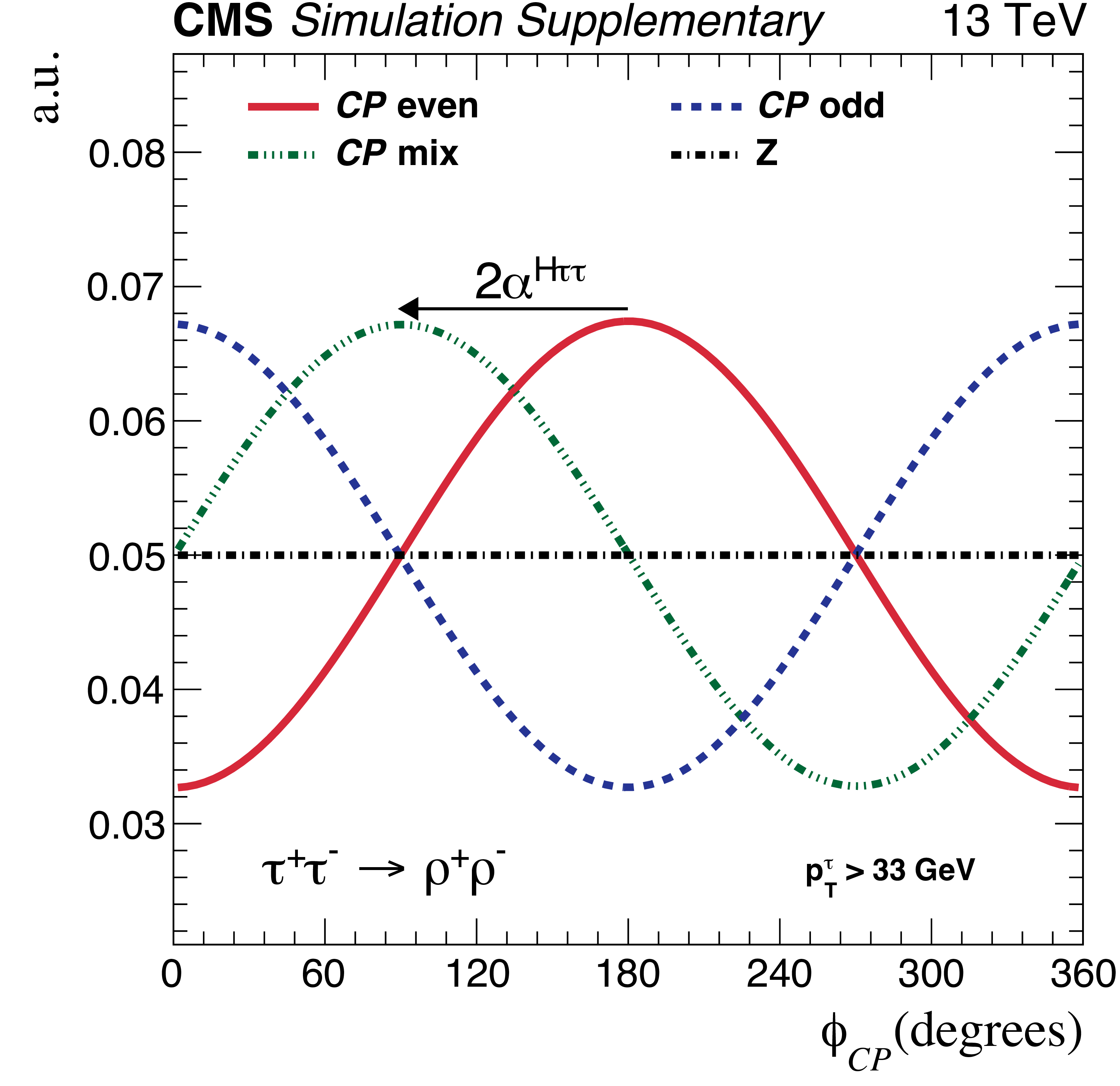
png pdf	Figure 2: The normalised distribution of ${\phi _{{\textit {CP}}}}$ between the $\tau$ lepton decay planes in the H rest frame at the generator level, for both $\tau$ leptons decaying to a charged pion and a neutrino. The distributions are for a decaying scalar (CP-even, solid red), pseudoscalar (CP-odd, dash blue), a maximal mixing angle of $45^{\circ}$ (CP-mix, dash-dot-dot green), and a Z vector boson (black dash-dot). The transverse momentum of the visible $\tau$ decay products $ {p_{\mathrm {T}}} ^{\tau}$ was required to be larger than 33 GeV during the event generation.
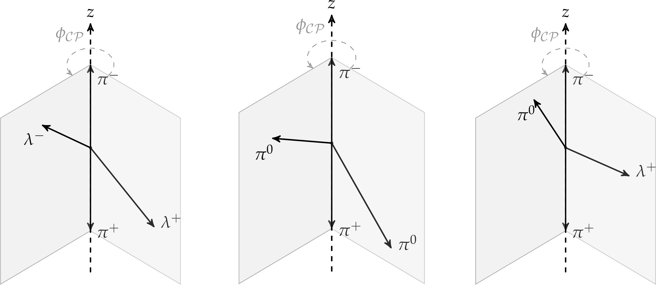
png pdf	Figure 3: Illustration of the $\tau$ lepton decay planes and the angle ${\phi _{{\textit {CP}}}}$ for various decay configurations. The decay planes are illustrated with the shaded regions, and either the vector ${\hat{\lambda}}$ or the momentum vector of the neutral pion is in the decay plane. The illustrations are in the frame in which the sum of the momenta of the charged particles is zero. Left: the decay plane for the decays $\tau^{-} \to \pi^{-} +\nu $ and $\tau^{+} \to \pi^{+} +\bar{\nu} $. Middle: the decay plane as reconstructed from the neutral and charged pion momenta. Right: ${\phi _{{\textit {CP}}}}$ for the mixed scenario, in which one $\tau$ lepton decays to a pion while the other decays via an intermediate $\rho$ meson.
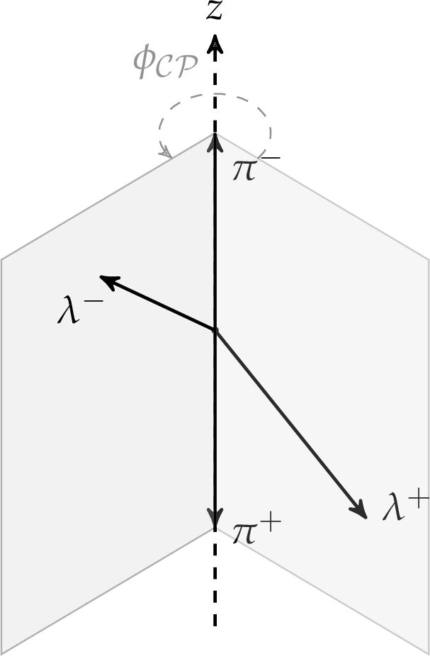
png pdf	Figure 3-a: The decay plane for the decays $\tau^{-} \to \pi^{-} +\nu $ and $\tau^{+} \to \pi^{+} +\bar{\nu} $.
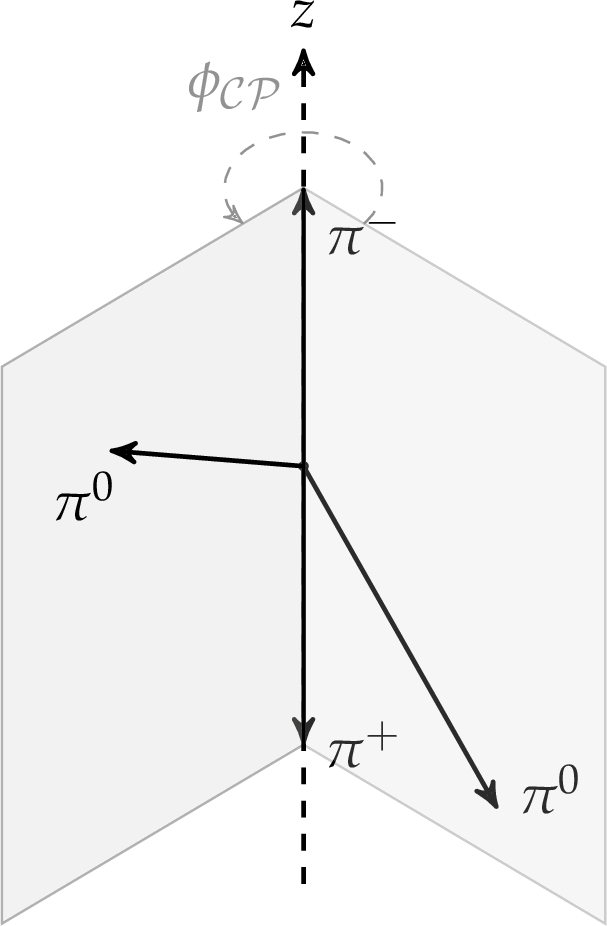
png pdf	Figure 3-b: The decay plane as reconstructed from the neutral and charged pion momenta.
png pdf	Figure 3-c: ${\phi _{{\textit {CP}}}}$ for the mixed scenario, in which one $\tau$ lepton decays to a pion while the other decays via an intermediate $\rho$ meson.
png pdf	Figure 4: The decay of ${\mathrm {a_{1}^{3\text{pr}}}}$ via an intermediate ${\rho ^0}$ to three charged pions.
png pdf	Figure 5: The angle ${\phi _{{\textit {CP}}}}$ for ${\mu \to {\tau _\mathrm {h}}}$ events in which the ${\tau _\mathrm {h}}$ decays to a charged $\pi$ (upper) or a charged $\rho$ meson (lower). The distributions are decomposed in a subset in which the charged $\pi$ is "nearly coplanar" (left) or "nearly perpendicular" (right) to the production plane.
png pdf	Figure 5-a: The angle ${\phi _{{\textit {CP}}}}$ for ${\mu \to {\tau _\mathrm {h}}}$ events in which the ${\tau _\mathrm {h}}$ decays to a charged $\pi$. In this subset the charged $\pi$ is "nearly coplanar" to the production plane.
png pdf	Figure 5-b: The angle ${\phi _{{\textit {CP}}}}$ for ${\mu \to {\tau _\mathrm {h}}}$ events in which the ${\tau _\mathrm {h}}$ decays to a charged $\rho$ meson. In this subset the charged $\pi$ is "nearly perpendicular" to the production plane.
png pdf	Figure 5-c: The angle ${\phi _{{\textit {CP}}}}$ for ${\mu \to {\tau _\mathrm {h}}}$ events in which the ${\tau _\mathrm {h}}$ decays to a charged $\pi$ (upper) or a charged $\rho$ meson (lower). The distributions are decomposed in a subset in which the charged $\pi$ is "nearly coplanar" (left) or "nearly perpendicular" (right) to the production plane.
png pdf	Figure 5-d: The angle ${\phi _{{\textit {CP}}}}$ for ${\mu \to {\tau _\mathrm {h}}}$ events in which the ${\tau _\mathrm {h}}$ decays to a charged $\pi$ (upper) or a charged $\rho$ meson (lower). The distributions are decomposed in a subset in which the charged $\pi$ is "nearly coplanar" (left) or "nearly perpendicular" (right) to the production plane.
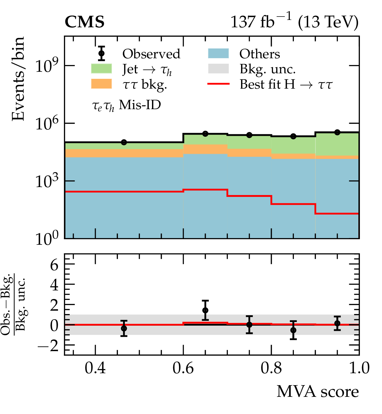
png pdf	Figure 6: The post-fit MVA score distributions for the Genuine (left) and Mis-ID categories (right) in the ${\tau _{\mu} {\tau _\mathrm {h}}}$ (upper) and ${{\tau _{\mathrm{e}}} {\tau _\mathrm {h}}}$ (lower) channels. The distributions are inclusive in ${\tau _\mathrm {h}}$ decay mode. The best fit signal distributions are overlaid. In the lower panels, the data minus the background template divided by the uncertainty in the background template is displayed, as well as the signal distribution divided by the uncertainty in the background template. The uncertainty band accounts for all sources of systematic uncertainty in the background prediction, after the fit to data.
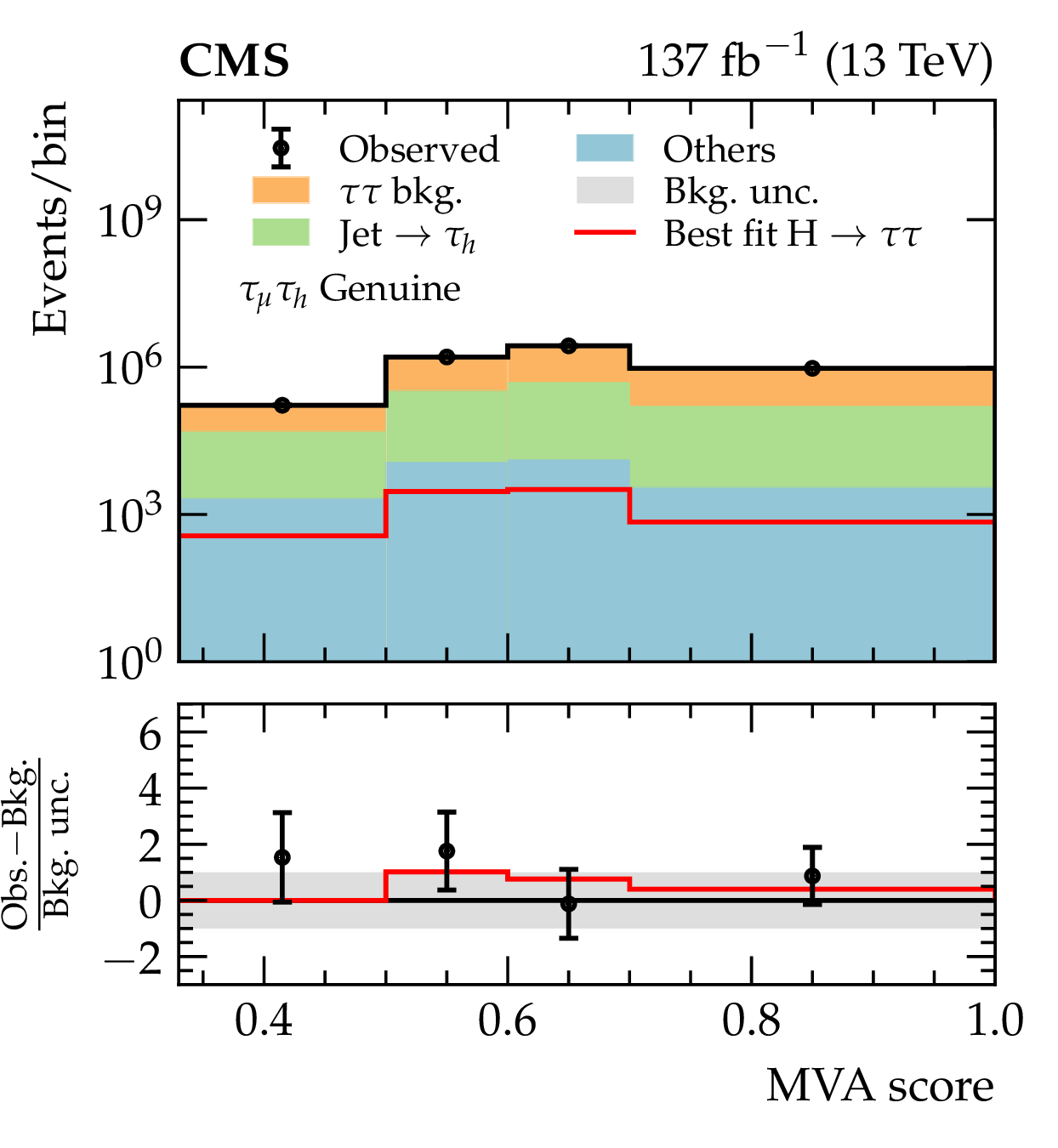
png pdf	Figure 6-a: The post-fit MVA score distribution for the Genuine category in the ${\tau _{\mu} {\tau _\mathrm {h}}}$ channel. The distribution is inclusive in ${\tau _\mathrm {h}}$ decay mode. The best fit signal distribution is overlaid. In the lower panel, the data minus the background template divided by the uncertainty in the background template is displayed, as well as the signal distribution divided by the uncertainty in the background template. The uncertainty band accounts for all sources of systematic uncertainty in the background prediction, after the fit to data.
png pdf	Figure 6-b: The post-fit MVA score distribution for the Mis-ID category in the ${\tau _{\mu} {\tau _\mathrm {h}}}$ channel. The distribution is inclusive in ${\tau _\mathrm {h}}$ decay mode. The best fit signal distribution is overlaid. In the lower panel, the data minus the background template divided by the uncertainty in the background template is displayed, as well as the signal distribution divided by the uncertainty in the background template. The uncertainty band accounts for all sources of systematic uncertainty in the background prediction, after the fit to data.
png pdf	Figure 6-c: The post-fit MVA score distribution for the Genuine category in the ${{\tau _{\mathrm{e}}} {\tau _\mathrm {h}}}$ channel. The distribution is inclusive in ${\tau _\mathrm {h}}$ decay mode. The best fit signal distribution is overlaid. In the lower panel, the data minus the background template divided by the uncertainty in the background template is displayed, as well as the signal distribution divided by the uncertainty in the background template. The uncertainty band accounts for all sources of systematic uncertainty in the background prediction, after the fit to data.
png pdf	Figure 6-d: The post-fit MVA score distribution for the Mis-ID category in the ${{\tau _{\mathrm{e}}} {\tau _\mathrm {h}}}$ channel. The distribution is inclusive in ${\tau _\mathrm {h}}$ decay mode. The best fit signal distribution is overlaid. In the lower panel, the data minus the background template divided by the uncertainty in the background template is displayed, as well as the signal distribution divided by the uncertainty in the background template. The uncertainty band accounts for all sources of systematic uncertainty in the background prediction, after the fit to data.
png pdf	Figure 7: The post-fit MVA score distributions for the Genuine (left) and Mis-ID categories (right) in the ${{\tau _\mathrm {h}} {\tau _\mathrm {h}}}$ channel. The distributions are inclusive in ${\tau _\mathrm {h}}$ decay mode. The best fit signal distributions are overlaid. In the lower panels, the data minus the background template divided by the uncertainty in the background template is displayed, as well as the signal distribution divided by the uncertainty in the background template. The uncertainty band accounts for all sources of systematic uncertainty in the background prediction, after the fit to data.
png pdf	Figure 7-a: The post-fit MVA score distribution for the Genuine category in the ${{\tau _\mathrm {h}} {\tau _\mathrm {h}}}$ channel. The distribution is inclusive in ${\tau _\mathrm {h}}$ decay mode. The best fit signal distribution is overlaid. In the lower panel, the data minus the background template divided by the uncertainty in the background template is displayed, as well as the signal distribution divided by the uncertainty in the background template. The uncertainty band accounts for all sources of systematic uncertainty in the background prediction, after the fit to data.
png pdf	Figure 7-b: The post-fit MVA score distribution for the Mis-ID category in the ${{\tau _\mathrm {h}} {\tau _\mathrm {h}}}$ channel. The distribution is inclusive in ${\tau _\mathrm {h}}$ decay mode. The best fit signal distribution is overlaid. In the lower panel, the data minus the background template divided by the uncertainty in the background template is displayed, as well as the signal distribution divided by the uncertainty in the background template. The uncertainty band accounts for all sources of systematic uncertainty in the background prediction, after the fit to data.
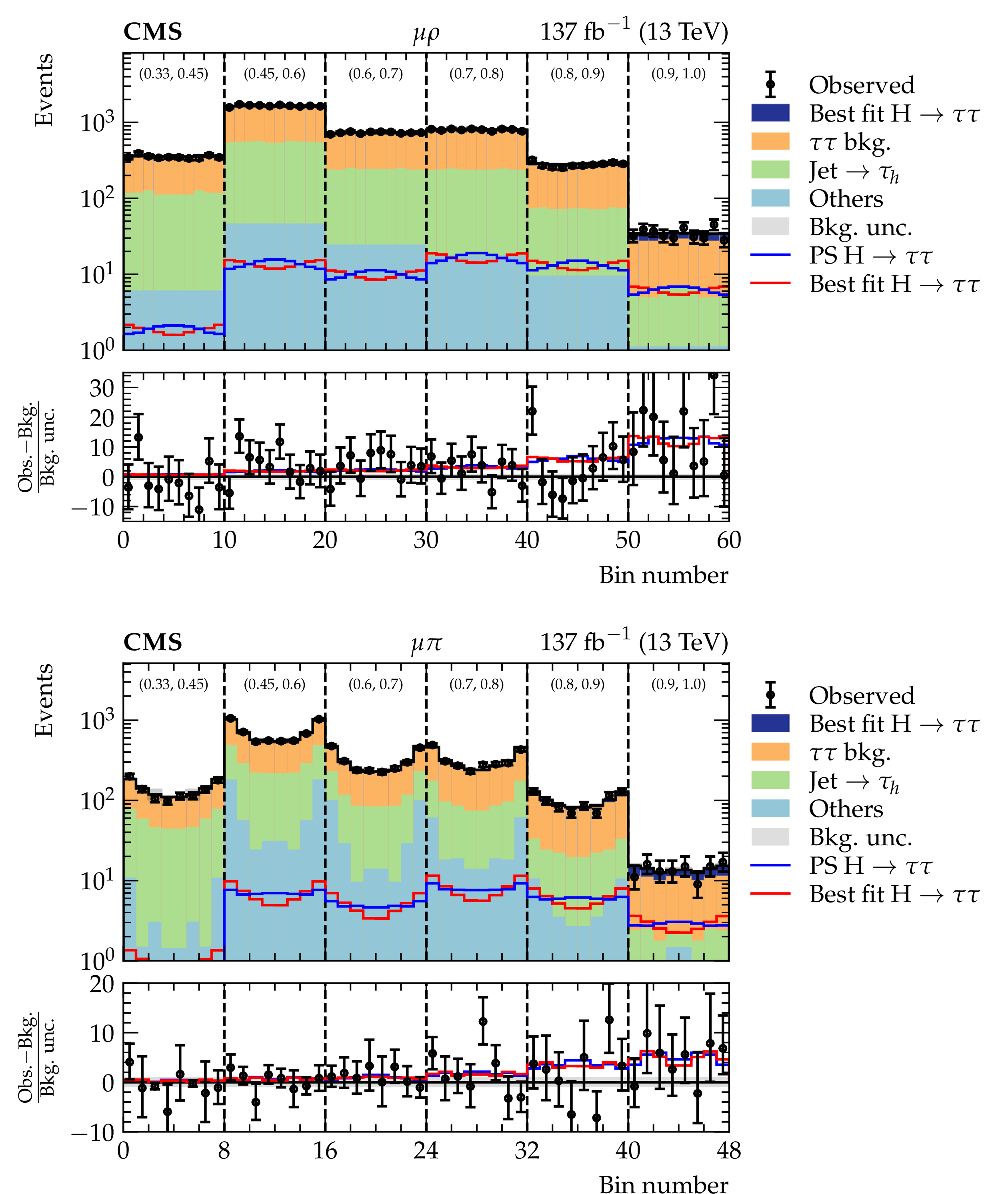
png pdf	Figure 8: Distributions of ${\phi _{{\textit {CP}}}}$ in the ${\mu \rho}$ (upper) and ${\mu \pi}$ (lower) channels in windows of increasing MVA score, shown on top of each window. The best fit and pseudoscalar (PS) signal distributions are overlaid. The $x$-axis represents the cyclic bins in ${\phi _{{\textit {CP}}}}$ in the range of $(0, 360^{\circ})$. In the lower panels, the data minus the background template divided by the uncertainty in the background template is displayed, as well as the signal distributions divided by the uncertainty in the background template. The uncertainty band accounts for all sources of systematic uncertainty in the background prediction, after the fit to data.
png pdf	Figure 8-a: Distribution of ${\phi _{{\textit {CP}}}}$ in the ${\mu \rho}$ channel in windows of increasing MVA score, shown on top of the window. The best fit and pseudoscalar (PS) signal distributions are overlaid. The $x$-axis represents the cyclic bins in ${\phi _{{\textit {CP}}}}$ in the range of $(0, 360^{\circ})$. In the lower panel, the data minus the background template divided by the uncertainty in the background template is displayed, as well as the signal distributions divided by the uncertainty in the background template. The uncertainty band accounts for all sources of systematic uncertainty in the background prediction, after the fit to data.
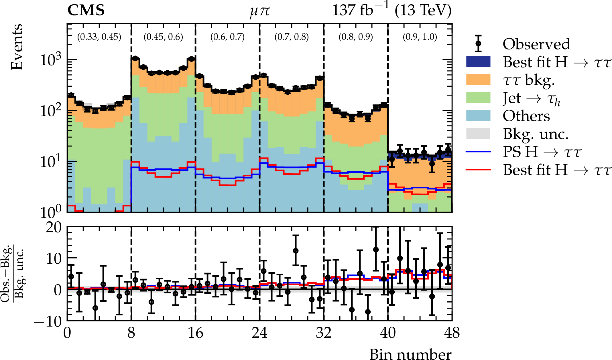
png pdf	Figure 8-b: Distribution of ${\phi _{{\textit {CP}}}}$ in the ${\mu \pi}$ channel in windows of increasing MVA score, shown on top of the window. The best fit and pseudoscalar (PS) signal distributions are overlaid. The $x$-axis represents the cyclic bins in ${\phi _{{\textit {CP}}}}$ in the range of $(0, 360^{\circ})$. In the lower panel, the data minus the background template divided by the uncertainty in the background template is displayed, as well as the signal distributions divided by the uncertainty in the background template. The uncertainty band accounts for all sources of systematic uncertainty in the background prediction, after the fit to data.
png pdf	Figure 9: Distributions of ${\phi _{{\textit {CP}}}}$ in the ${\rho \rho}$ (upper) and ${\pi \rho}$ (lower) channels in windows of increasing MVA score, shown on top of each window. The best fit and pseudoscalar (PS) signal distributions are overlaid. The $x$-axis represents the cyclic bins in ${\phi _{{\textit {CP}}}}$ in the range of $(0, 360^{\circ})$. In the lower panels, the data minus the background template divided by the uncertainty in the background template is displayed, as well as the signal distributions divided by the uncertainty in the background template. The uncertainty band accounts for all sources of systematic uncertainty in the background prediction, after the fit to data.
png pdf	Figure 9-a: Distribution of ${\phi _{{\textit {CP}}}}$ in the ${\rho \rho}$ channel in windows of increasing MVA score, shown on top of the window. The best fit and pseudoscalar (PS) signal distributions are overlaid. The $x$-axis represents the cyclic bins in ${\phi _{{\textit {CP}}}}$ in the range of $(0, 360^{\circ})$. In the lower panel, the data minus the background template divided by the uncertainty in the background template is displayed, as well as the signal distributions divided by the uncertainty in the background template. The uncertainty band accounts for all sources of systematic uncertainty in the background prediction, after the fit to data.
png pdf	Figure 9-b: Distribution of ${\phi _{{\textit {CP}}}}$ in the ${\pi \rho}$ channel in windows of increasing MVA score, shown on top of the window. The best fit and pseudoscalar (PS) signal distributions are overlaid. The $x$-axis represents the cyclic bins in ${\phi _{{\textit {CP}}}}$ in the range of $(0, 360^{\circ})$. In the lower panel, the data minus the background template divided by the uncertainty in the background template is displayed, as well as the signal distributions divided by the uncertainty in the background template. The uncertainty band accounts for all sources of systematic uncertainty in the background prediction, after the fit to data.
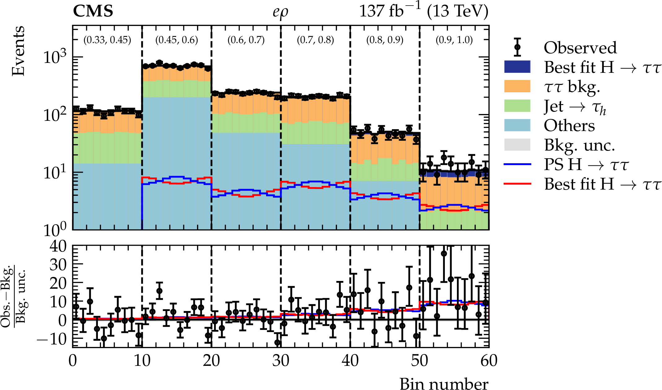
png pdf	Figure 10: Distributions of ${\phi _{{\textit {CP}}}}$ in the ${\mathrm{e} \rho}$ (upper) and ${\mathrm{e} \pi}$ (lower) channels in windows of increasing MVA score, shown on top of each window. The best fit and pseudoscalar (PS) signal distributions are overlaid. The $x$-axis represents the cyclic bins in ${\phi _{{\textit {CP}}}}$ in the range of $(0, 360^{\circ})$. In the lower panels, the data minus the background template divided by the uncertainty in the background template is displayed, as well as the signal distributions divided by the uncertainty in the background template. The uncertainty band accounts for all sources of systematic uncertainty in the background prediction, after the fit to data.
png pdf	Figure 10-a: Distribution of ${\phi _{{\textit {CP}}}}$ in the ${\mathrm{e} \rho}$ channel in windows of increasing MVA score, shown on top of the window. The best fit and pseudoscalar (PS) signal distributions are overlaid. The $x$-axis represents the cyclic bins in ${\phi _{{\textit {CP}}}}$ in the range of $(0, 360^{\circ})$. In the lower panel, the data minus the background template divided by the uncertainty in the background template is displayed, as well as the signal distributions divided by the uncertainty in the background template. The uncertainty band accounts for all sources of systematic uncertainty in the background prediction, after the fit to data.
png pdf	Figure 10-b: Distribution of ${\phi _{{\textit {CP}}}}$ in the ${\mathrm{e} \pi}$ channel in windows of increasing MVA score, shown on top of the window. The best fit and pseudoscalar (PS) signal distributions are overlaid. The $x$-axis represents the cyclic bins in ${\phi _{{\textit {CP}}}}$ in the range of $(0, 360^{\circ})$. In the lower panel, the data minus the background template divided by the uncertainty in the background template is displayed, as well as the signal distributions divided by the uncertainty in the background template. The uncertainty band accounts for all sources of systematic uncertainty in the background prediction, after the fit to data.
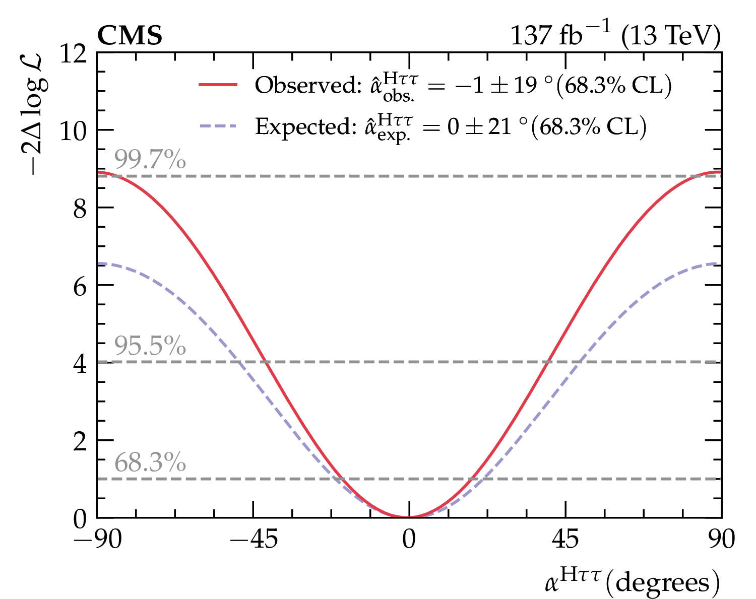
png pdf	Figure 11: Negative log-likelihood scan for the combination of the ${{\tau _{\mathrm{e}}} {\tau _\mathrm {h}}}$, ${\tau _{\mu} {\tau _\mathrm {h}}}$, and ${{\tau _\mathrm {h}} {\tau _\mathrm {h}}}$ channels. The observed (expected) sensitivity to distinguish between the scalar and pseudoscalar hypotheses, defined at $ {\alpha ^{\mathrm{H} \tau \tau}} = $ 0 and $ \pm 90 ^{\circ}$, respectively, is 3.0$\sigma $ (2.6$\sigma $). The observed (expected) value for ${\alpha ^{\mathrm{H} \tau \tau}}$ is $-1 \pm 19 ^{\circ}$ ($0 \pm 21 ^{\circ}$) at the 68.3% CL. At 95.5% CL the range is $ \pm 41 ^{\circ}$ ($ \pm 49 ^{\circ}$), and at the 99.7% CL the observed range is $ \pm 84 ^{\circ}$.
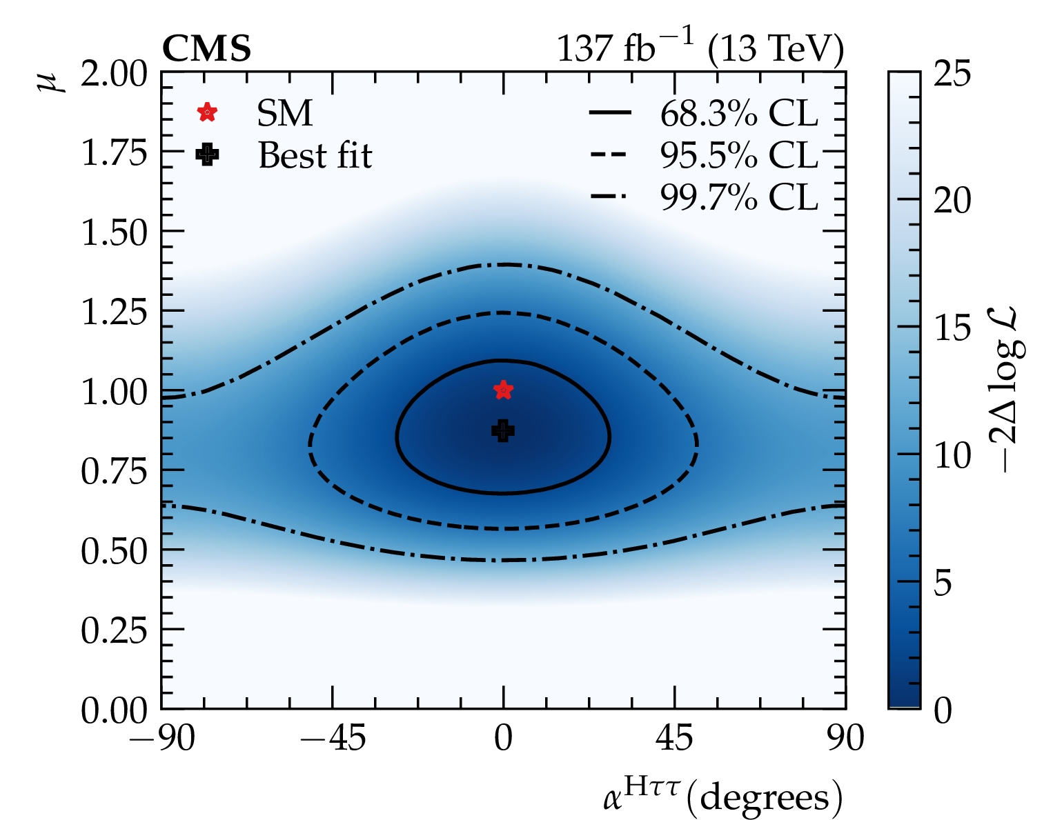
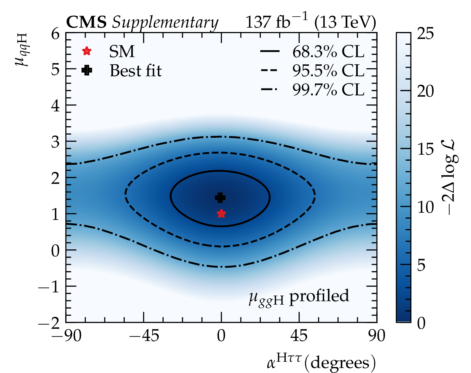
png pdf	Figure 12: The 2-D scan of the signal strength modifier $\mu $ versus ${\alpha ^{\mathrm{H} \tau \tau}}$. The 68.3, 95.5, and 99.7% confidence regions are overlaid.
png pdf	Figure 13: The 2-D scan of the (reduced) CP-even (${\kappa _\tau}$) and CP-odd (${\tilde{\kappa}_\tau}$) $\tau$ Yukawa couplings. The 68.3, 95.5, and 99.7% confidence regions are overlaid.
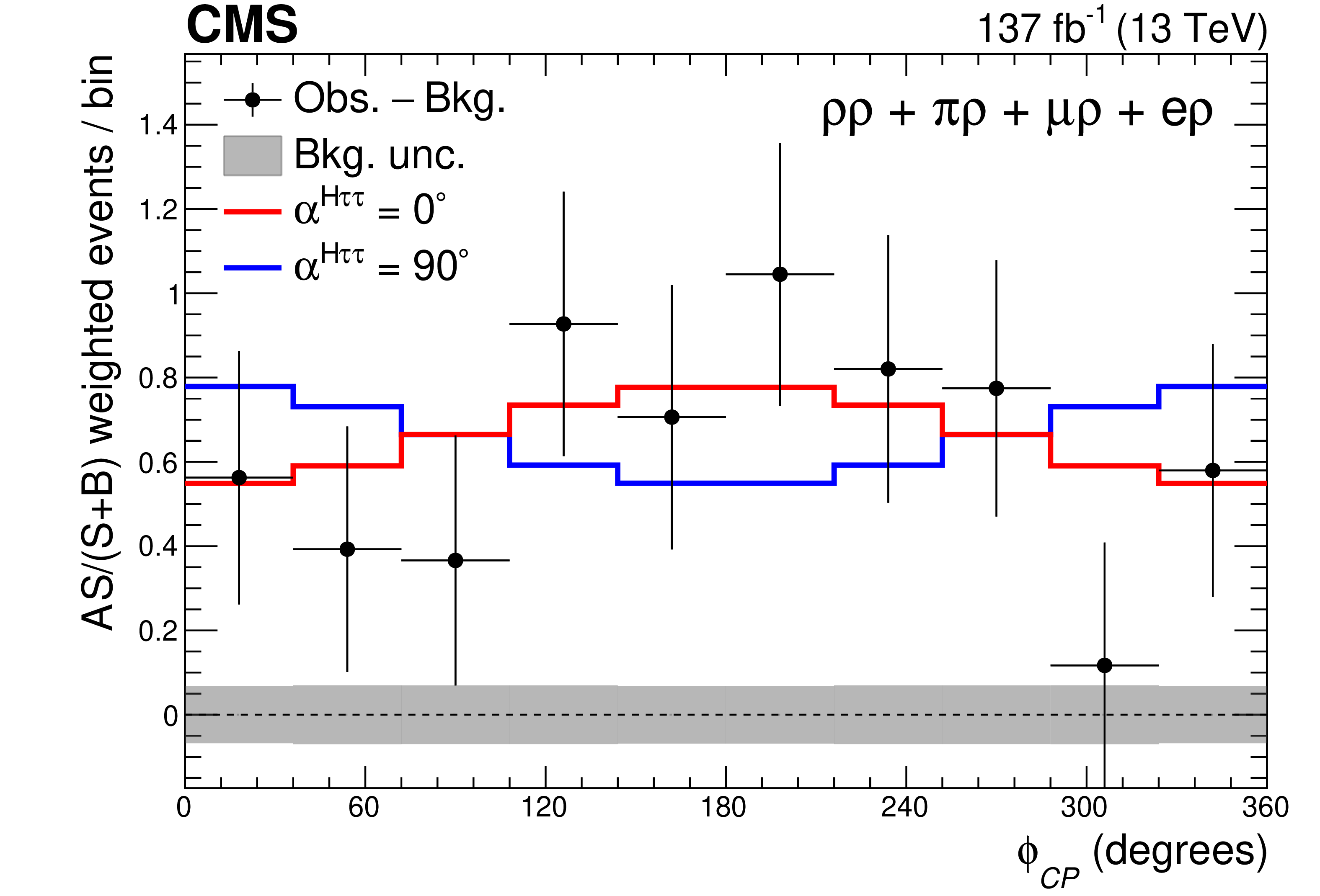
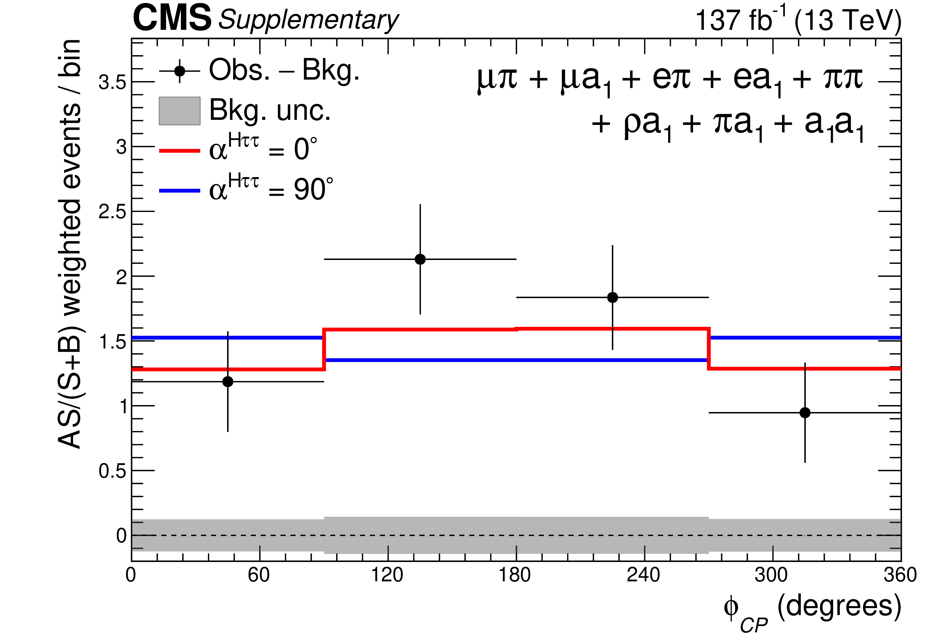
png pdf	Figure 14: The ${\phi _{{\textit {CP}}}}$ distributions for the ${\rho \rho}$, ${\pi \rho}$, ${\mu \rho}$, and ${\mathrm{e} \rho}$ channels weighed by A S/(S+B) are combined. Events are included from all MVA score bins in the four signal categories. The background is subtracted from the data. The scalar distribution is depicted in red, while the pseudoscalar is displayed in blue. In the predictions, the rate parameters are taken from their best fit values. The grey uncertainty band indicates the uncertainty in the subtracted background component. In combining the channels, a phase-shift of 180$^{\circ}$ was applied to the channels involving a lepton since this channel has a phase difference of 180$^{\circ}$ with respect to the two hadronic channels due to a sign-flip in the spectral function of the light lepton.

Tables
png pdf	Table 1: Decay modes of $\tau$ leptons used in this analysis and their branching fractions $\mathcal {B}$ [38]. Where appropriate, we indicate the known intermediate resonances. The last row gives the shorthand notation for the decays used throughout this paper.
png pdf	Table 2: Kinematic trigger and offline requirements applied to the ${{\tau _{\mathrm{e}}} {\tau _\mathrm {h}}}$, ${\tau _{\mu} {\tau _\mathrm {h}}}$, and ${{\tau _\mathrm {h}} {\tau _\mathrm {h}}}$ channels. The trigger ${p_{\mathrm {T}}}$ requirement is indicated in parentheses (in GeV). The ${p_{\mathrm {T}}}$ thresholds indicated for the ${\tau _\mathrm {h}}$ apply only for the object matched to the hadronic trigger or to the hadronic leg from the cross trigger.
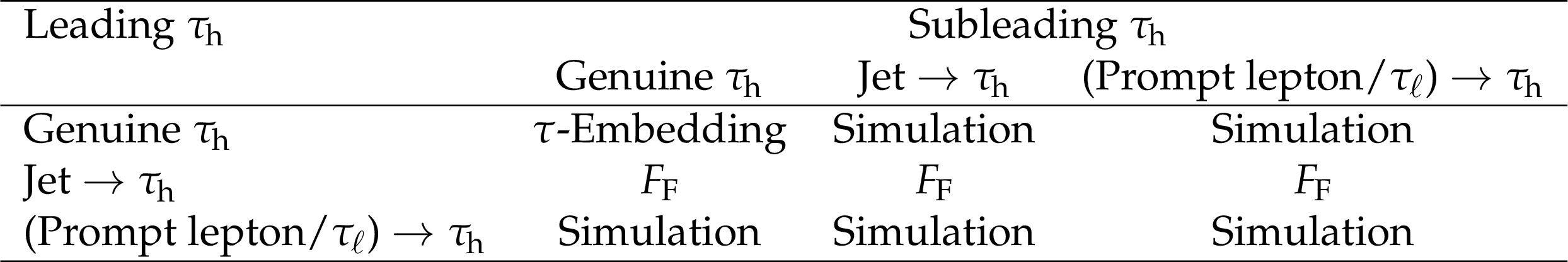
png pdf	Table 3: The different sources of backgrounds in the ${{\tau _\mathrm {h}} {\tau _\mathrm {h}}}$ channel are shown in the rows and columns. The entries in the table represent the possible $\tau$ lepton pair background contribution from different processes and misidentifications and encapsulate the different experimental techniques that are deployed to estimate the background contributions.
png pdf	Table 4: The different sources of backgrounds in the ${{\tau _{\ell}} {\tau _\mathrm {h}}}$ channel are shown in the rows and columns. The entries in the table represent the possible $\tau$ lepton pair background contribution from different processes and misidentifications and encapsulate the different experimental techniques that are deployed to estimate the background contributions.
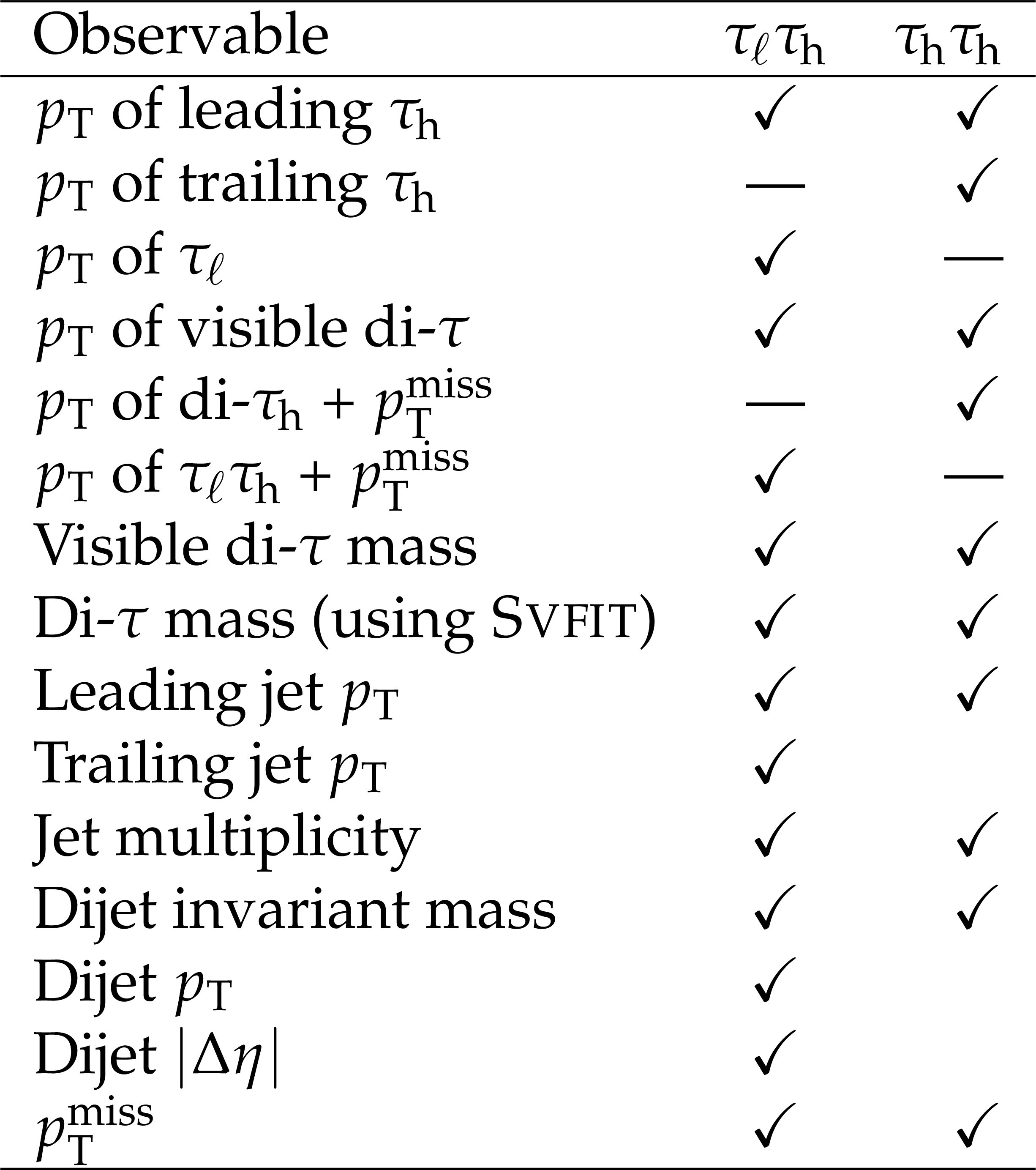
png pdf	Table 5: Input variables to the MVA discriminants for the ${{\tau _{\ell}} {\tau _\mathrm {h}}}$ and ${{\tau _\mathrm {h}} {\tau _\mathrm {h}}}$ channels. The {Svfit} algorithm is used to estimate the di-$\tau$ mass.
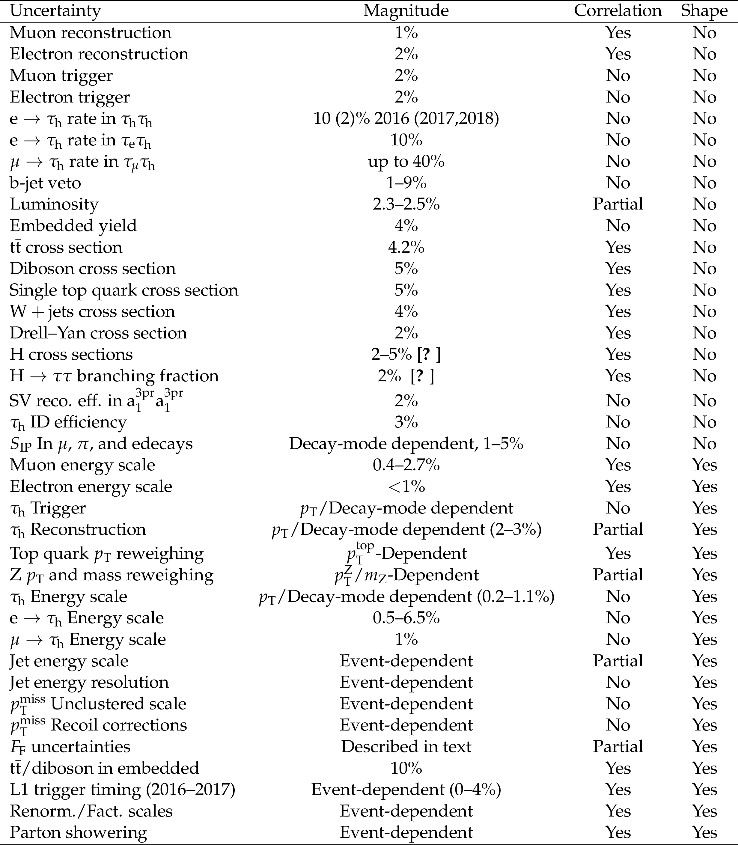
png pdf	Table 6: Overview of the systematic uncertainties. The third column indicates if the source of uncertainty was treated as being correlated between the years in the fit described in Section 12. The forth column indicates if the uncertainty affects the shapes of the distributions.

Summary

The first measurement of the effective mixing angle $\alpha^{\mathrm{H \to \tau\tau}}$ between scalar and pseudoscalar $\mathrm{H\tau\tau}$ couplings has been presented for a data set of proton-proton collisions at $\sqrt{s} = $ 13 TeV corresponding to an integrated luminosity of 137 fb$^{-1}$. The data were collected with the CMS experiment at the LHC in the period 2016-2018. The following $\tau$ lepton decay modes were included: $\mathrm{e^{\pm}}$, $\mu^{\pm}$, $\pi^{\pm}$, $\rho^{\pm} \to \pi^{\pm}\pi^{0}$, $\mathrm{q}_{1}^\pm\to\pi^{\pm}\pi^{0}\pi^{0}$, and $\mathrm{q}_{1}^\pm\to\pi^{\pm}\pi^{\mp}\pi^{\pm}$. Dedicated strategies were adopted to reconstruct the angle $\phi_{\text{CP}}$ between the $\tau$ decay planes for the various $\tau$ decay modes. The data disfavour the pure CP-odd scenario at 3.0 standard deviations. The observed effective mixing angle is found to be $-1 \pm 19 ^{\circ}$, while the expected value is $0 \pm 21 ^{\circ}$ at the 68.3% confidence level (CL). The observed and expected uncertainties are found to be $ \pm 41 ^{\circ}$ and $ \pm 49 ^{\circ}$ at the 95.5% CL, respectively, and the observed sensitivity at the 99.7% CL is $ \pm 84 ^{\circ}$. The leading uncertainty in the measurement is statistical, implying that the precision of the measurement will increase with the accumulation of more collision data. The measurement is consistent with the standard model expectation, and reduces the allowed parameter space for its extensions. Tabulated results are provided in HEPDATA [110].

Additional Figures
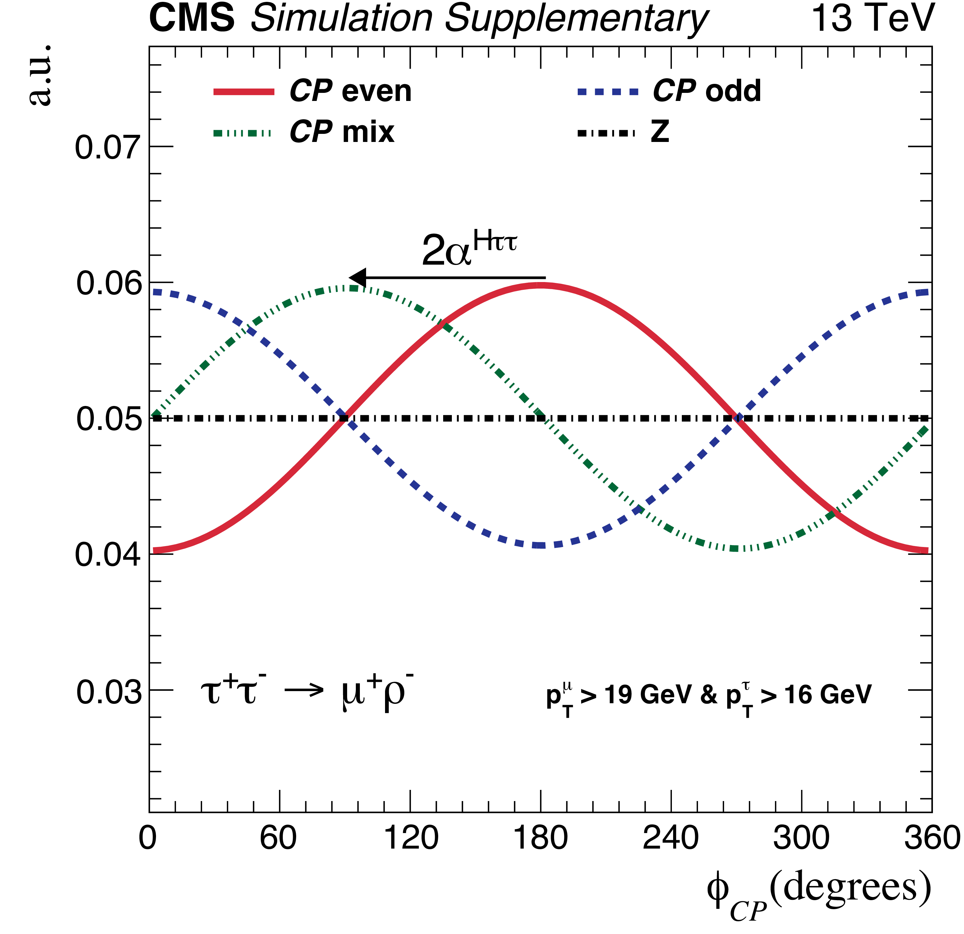
png pdf	Additional Figure 1: The normalised distribution of $\phi _{\textit {CP}}$ between the ${\tau}$ decay planes in the visible rest frame in the $ {{\mu}} {\pi}$ channel. The distributions are for a decaying scalar (CP-even, solid red), pseudoscalar (CP-odd, dash blue), a maximal mixing angle of 45$^{\circ}$ (CP-mix, dash-dot-dot green), and a Z vector boson (black dash-dot). A ${p_{\mathrm {T}}}$ cutoff of 19 (16) GeV is applied on the visible leptonic (hadronic) tau decay products.
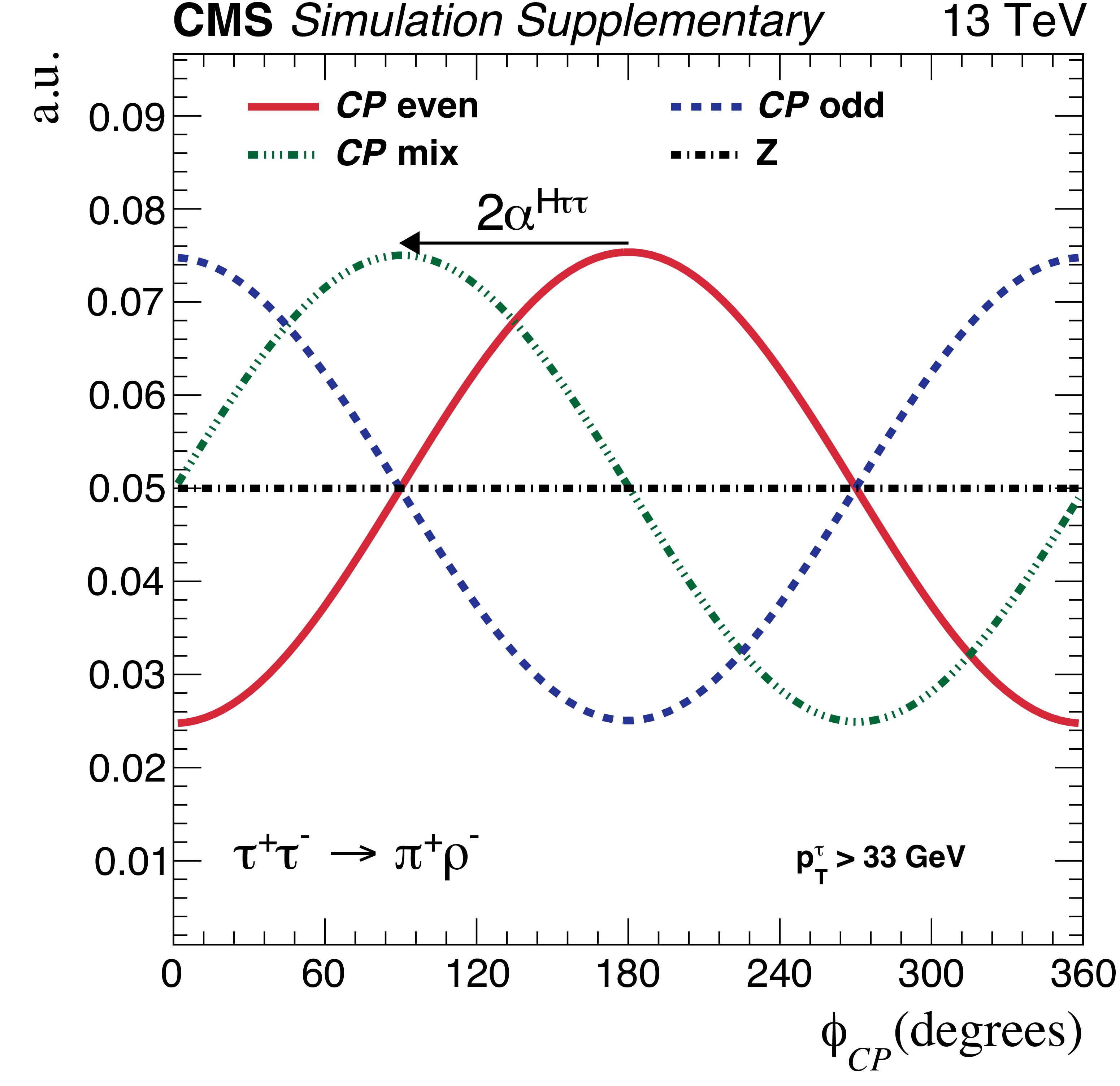
png pdf	Additional Figure 2: The normalised distribution of $\phi _{\textit {CP}}$ between the ${\tau}$ decay planes in the visible rest frame in the $ {\pi} {\rho} $ channel. The distributions are for a decaying scalar (CP-even, solid red), pseudoscalar (CP-odd, dash blue), a maximal mixing angle of 45$^{\circ}$ (CP-mix, dash-dot-dot green), and a Z vector boson (black dash-dot). A ${p_{\mathrm {T}}}$ cutoff of 33 GeV is applied on the visible tau decay products.
png pdf	Additional Figure 3: The normalised distribution of $\phi _{\textit {CP}}$ between the ${\tau}$ decay planes in visible rest frame in the $ {\rho} {\rho} $ channel. The distributions are for a decaying scalar (CP-even, solid red), pseudoscalar (CP-odd, dash blue), a maximal mixing angle of 45$^{\circ}$ (CP-mix, dash-dot-dot green), and a Z vector boson (black dash-dot). A ${p_{\mathrm {T}}}$ cutoff of 33 GeV is applied on the visible tau decay products.
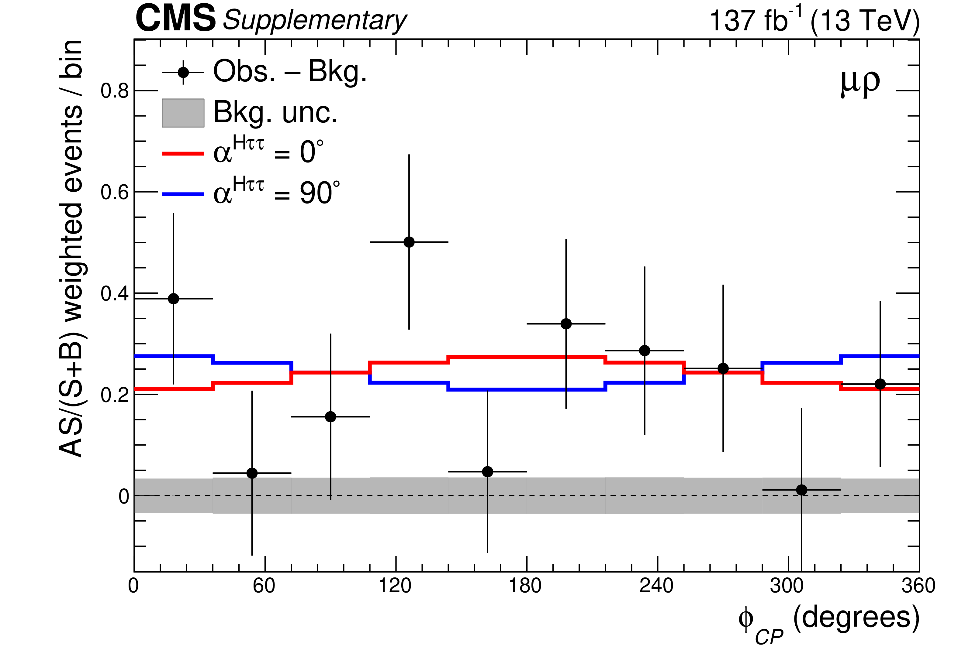
png pdf	Additional Figure 4: The $\phi _{\textit {CP}}$ distribution in the $ {{\mu}} {\rho} $ channel. Events were collected from all years and MVA score bins. The background is subtracted from the data. The events are reweighed via AS/(S+B), in which S and B are the signal and background rates, respectively, and A is a measure for the average asymmetry between the scalar and pseudoscalar distributions. The definition of the value of A per bin is $ {| \textit {CP}^{\text {even}}-\textit {CP}^{\text {odd}} |}/(\textit {CP}^{\text {even}}+\textit {CP}^{\text {odd}})$, and A is normalised to the total number of bins. In this equation $\textit {CP}^{\text {even}}$ and $\textit {CP}^{\text {odd}}$ are the scalar and pseudoscalar contributions per bin. The scalar distribution is depicted in red, while the pseudoscalar is displayed in blue. In the predictions the rate parameters are taken from their best fit values. The grey uncertainty band indicates the uncertainty in the subtracted background component. It should be noted that an overall phase-shift of 180$^{\circ}$ was applied to the channel.
png pdf	Additional Figure 5: The $\phi _{\textit {CP}}$ distribution in the $ {\pi} {\rho} $ channel. Events were collected from all years and MVA score bins. The background is subtracted from the data. The events are reweighed via AS/(S+B), in which S and B are the signal and background rates, respectively, and A is a measure for the average asymmetry between the scalar and pseudoscalar distributions. The definition of the value of A per bin is $ {| \textit {CP}^{\text {even}}-\textit {CP}^{\text {odd}} |}/(\textit {CP}^{\text {even}}+\textit {CP}^{\text {odd}})$, and A is normalised to the total number of bins. In this equation $\textit {CP}^{\text {even}}$ and $\textit {CP}^{\text {odd}}$ are the scalar and pseudoscalar contributions per bin. The scalar distribution is depicted in red, while the pseudoscalar is displayed in blue. In the predictions the rate parameters are taken from their best fit values. The grey uncertainty band indicates the uncertainty in the subtracted background component.
png pdf	Additional Figure 6: The $\phi _{\textit {CP}}$ distribution in the $ {\rho} {\rho} $ channel. Events were collected from all years and MVA score bins. The background is subtracted from the data. The events are reweighed via AS/(S+B), in which S and B are the signal and background rates, respectively, and A is a measure for the average asymmetry between the scalar and pseudoscalar distributions. The definition of the value of A per bin is $ {| \textit {CP}^{\text {even}}-\textit {CP}^{\text {odd}} |}/(\textit {CP}^{\text {even}}+\textit {CP}^{\text {odd}})$, and A is normalised to the total number of bins. In this equation $\textit {CP}^{\text {even}}$ and $\textit {CP}^{\text {odd}}$ are the scalar and pseudoscalar contributions per bin. The scalar distribution is depicted in red, while the pseudoscalar is displayed in blue. In the predictions the rate parameters are taken from their best fit values. The grey uncertainty band indicates the uncertainty in the subtracted background component.
png pdf	Additional Figure 7: The $\phi _{\textit {CP}}$ distribution in the $ {\mathrm {e}} {\rho} $ channel. Events were collected from all years and MVA score bins. The background is subtracted from the data. The events are reweighed via AS/(S+B), in which S and B are the signal and background rates, respectively, and A is a measure for the average asymmetry between the scalar and pseudoscalar distributions. The definition of the value of A per bin is $ {| \textit {CP}^{\text {even}}-\textit {CP}^{\text {odd}} |}/(\textit {CP}^{\text {even}}+\textit {CP}^{\text {odd}})$, and A is normalised to the total number of bins. In this equation $\textit {CP}^{\text {even}}$ and $\textit {CP}^{\text {odd}}$ are the scalar and pseudoscalar contributions per bin. The scalar distribution is depicted in red, while the pseudoscalar is displayed in blue. In the predictions the rate parameters are taken from their best fit values. The grey uncertainty band indicates the uncertainty in the subtracted background component. It should be noted that an overall phase-shift of 180$^{\circ}$ was applied to the channel.
png pdf	Additional Figure 8: The $\phi _{\textit {CP}}$ distribution for combination of the 13 least sensitive $\tau _{l}\tau _{\mathrm {h}}$ and $\tau _{\mathrm {h}}\tau _{\mathrm {h}}$ channels added together. Events were collected from all years and MVA score bins. The background is subtracted from the data. The events are reweighed via AS/(S+B), in which S and B are the signal and background rates, respectively, and A is a measure for the average asymmetry between the scalar and pseudoscalar distributions. The definition of the value of A per bin is $ {| \textit {CP}^{\text {even}}-\textit {CP}^{\text {odd}} |}/(\textit {CP}^{\text {even}}+\textit {CP}^{\text {odd}})$, and A is normalised to the total number of bins. In this equation $\textit {CP}^{\text {even}}$ and $\textit {CP}^{\text {odd}}$ are the scalar and pseudoscalar contributions per bin. The scalar distribution is depicted in red, while the pseudoscalar is displayed in blue. In the predictions the rate parameters are taken from their best fit values. The grey uncertainty band indicates the uncertainty in the subtracted background component. In combining the channels, a phase-shift of 180$^{\circ}$ was applied to a subset of the channels such that the distributions are all in phase.
png pdf	Additional Figure 9: Distributions of $\phi _{\textit {CP}}$ in the $ {{\mu}}\mathrm {a_{1}^{3pr}}$ channel for an event sample dominated by Drell-Yan events. Events were selected for which $\alpha ^{\rho}_{-}\geq \pi /4$ for the intermediate ${\rho}$. The Drell-Yan background template is extracted from simulation, while the $\text {jet}\to \tau _{\mathrm {h}}$ background is obtained from the $F_{\text {F}}$ method. The remaining backgrounds are summarised in the template named Other. In the lower plot the ratio between data and the prediction is displayed together with the systematic uncertainty band.
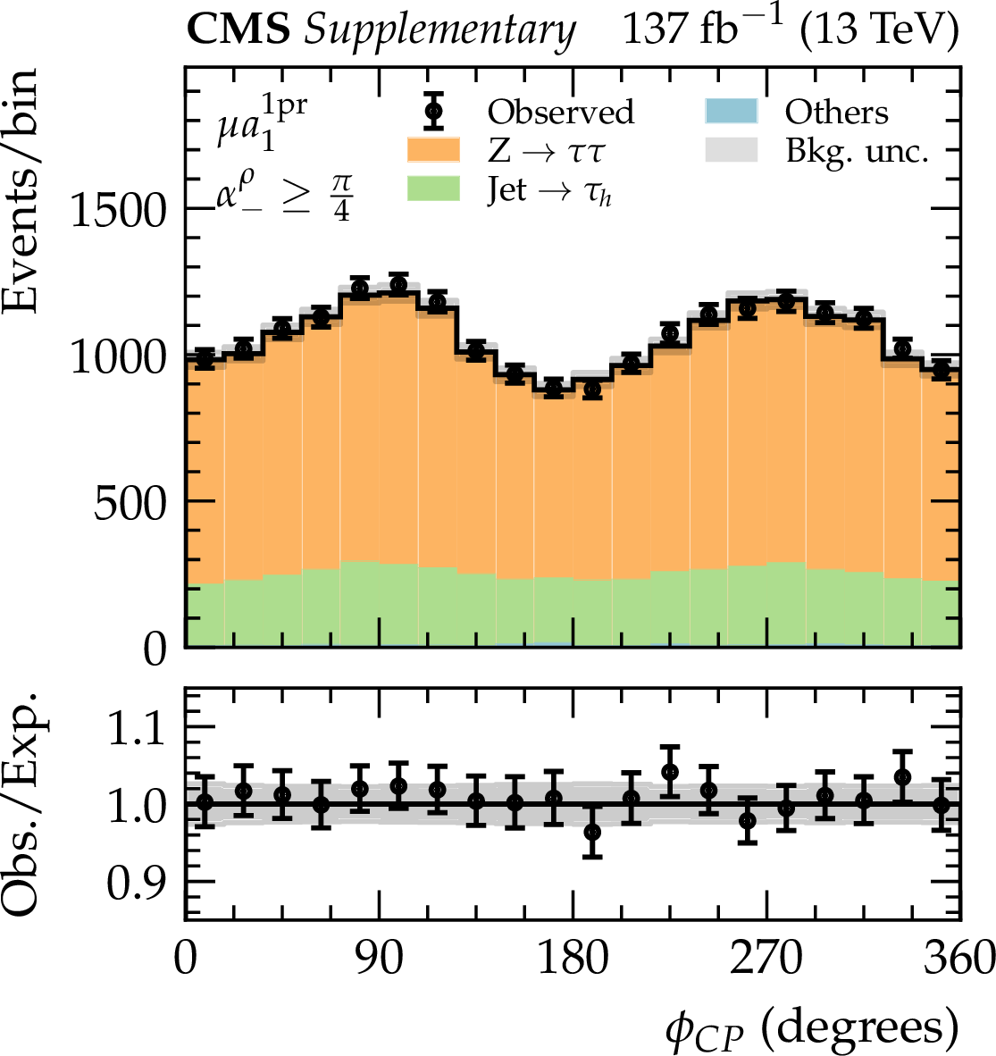
png pdf	Additional Figure 10: Distributions of $\phi _{\textit {CP}}$ in the $ {{\mu}}\mathrm {a_{1}^{1pr}}$ channel for an event sample dominated by Drell-Yan events. Events were selected for which $\alpha ^{\rho}_{-}$, calculated for the intermediate $\mathrm {a_{1}^{1pr}}$, was $\geq \pi /4$. The Drell-Yan background template is extracted from simulation, while the $\text {jet}\to \tau _{\mathrm {h}}$ background is obtained from the $F_{\text {F}}$ method. The remaining backgrounds are summarised in the template named Other. In the lower plot the ratio between data and the prediction is displayed together with the systematic uncertainty band.
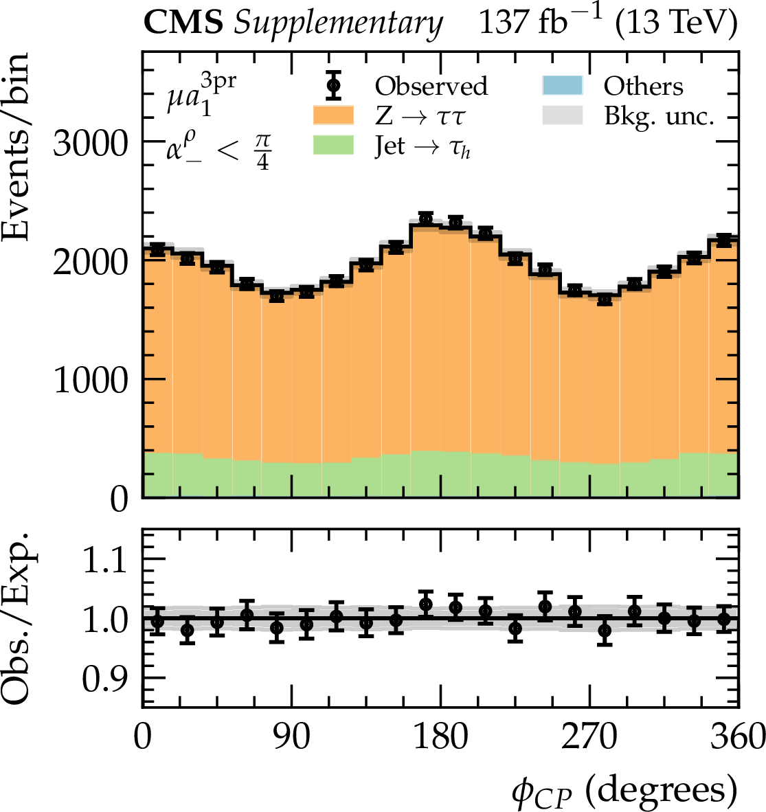
png pdf	Additional Figure 11: Distributions of $\phi _{\textit {CP}}$ in the $ {{\mu}}\mathrm {a_{1}^{3pr}}$ channel for an event sample dominated by Drell-Yan events. Events were selected for which $\alpha ^{\rho}_{-} < \pi /4$ for the intermediate ${\rho}$. The Drell-Yan background template is extracted from simulation, while the $\text {jet}\to \tau _{\mathrm {h}}$ background is obtained from the $F_{\text {F}}$ method. The remaining backgrounds are summarised in the template named Other. In the lower plot the ratio between data and the prediction is displayed together with the systematic uncertainty band.
png pdf	Additional Figure 12: Distributions of $\phi _{\textit {CP}}$ in the $ {{\mu}}\mathrm {a_{1}^{1pr}}$ channel for an event sample dominated by Drell-Yan events. Events were selected for which $\alpha ^{\rho}_{-}$, calculated for the intermediate $\mathrm {a_{1}^{1pr}}$, was $ < \pi /4$. The Drell-Yan background template is extracted from simulation, while the $\text {jet}\to \tau _{\mathrm {h}}$ background is obtained from the $F_{\text {F}}$ method. The remaining backgrounds are summarised in the template named Other. In the lower plot the ratio between data and the prediction is displayed together with the systematic uncertainty band.
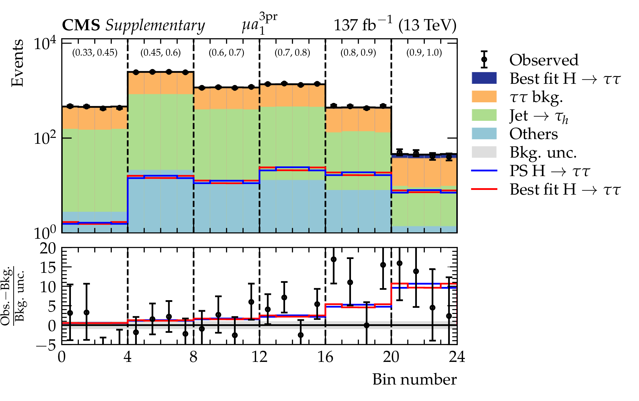
png pdf	Additional Figure 13: Distributions of $\phi _{\textit {CP}}$ in the $ {{\mu}}\mathrm {a_{1}^{3pr}}$ channel in windows of increasing MVA score, shown on top of each window. The best fit and pseudoscalar signal distributions are overlaid. The $x$ axis represents the cyclic bins in $\phi _{\textit {CP}}$ in the range of (0, 360$^{\circ}$). In the bottom plot the data minus the background template divided by the uncertainty in the background template is displayed, as well as the signal distributions divided by the uncertainty in the background template. The uncertainty band consists of the sum of the post-fit uncertainties in the background templates.
png pdf	Additional Figure 14: Distributions of $\phi _{\textit {CP}}$ in the $ {{\mu}}\mathrm {a_{1}^{1pr}}$ channel in windows of increasing MVA score, shown on top of each window. The best fit and pseudoscalar signal distributions are overlaid. The $x$ axis represents the cyclic bins in $\phi _{\textit {CP}}$ in the range of (0, 360$^{\circ}$). In the bottom plot the data minus the background template divided by the uncertainty in the background template is displayed, as well as the signal distributions divided by the uncertainty in the background template. The uncertainty band consists of the sum of the post-fit uncertainties in the background templates.
png pdf	Additional Figure 15: Distributions of $\phi _{\textit {CP}}$ in the $\mathrm {a_{1}^{1pr}} {\rho} +\mathrm {a_{1}^{1pr}}\mathrm {a_{1}^{1pr}}$ channels in windows of increasing MVA score, shown on top of each window. The best fit and pseudoscalar signal distributions are overlaid. The $x$ axis represents the cyclic bins in $\phi _{\textit {CP}}$ in the range of (0, 360$^{\circ}$). In the bottom plot the data minus the background template divided by the uncertainty in the background template is displayed, as well as the signal distributions divided by the uncertainty in the background template. The uncertainty band consists of the sum of the post-fit uncertainties in the background templates.
png pdf	Additional Figure 16: Distributions of $\phi _{\textit {CP}}$ in the $\mathrm {a_{1}^{3pr}}\mathrm {a_{1}^{1pr}}$ channel in windows of increasing MVA score, shown on top of each window. The best fit and pseudoscalar signal distributions are overlaid. The $x$ axis represents the cyclic bins in $\phi _{\textit {CP}}$ in the range of (0, 360$^{\circ}$). In the bottom plot the data minus the background template divided by the uncertainty in the background template is displayed, as well as the signal distributions divided by the uncertainty in the background template. The uncertainty band consists of the sum of the post-fit uncertainties in the background templates.
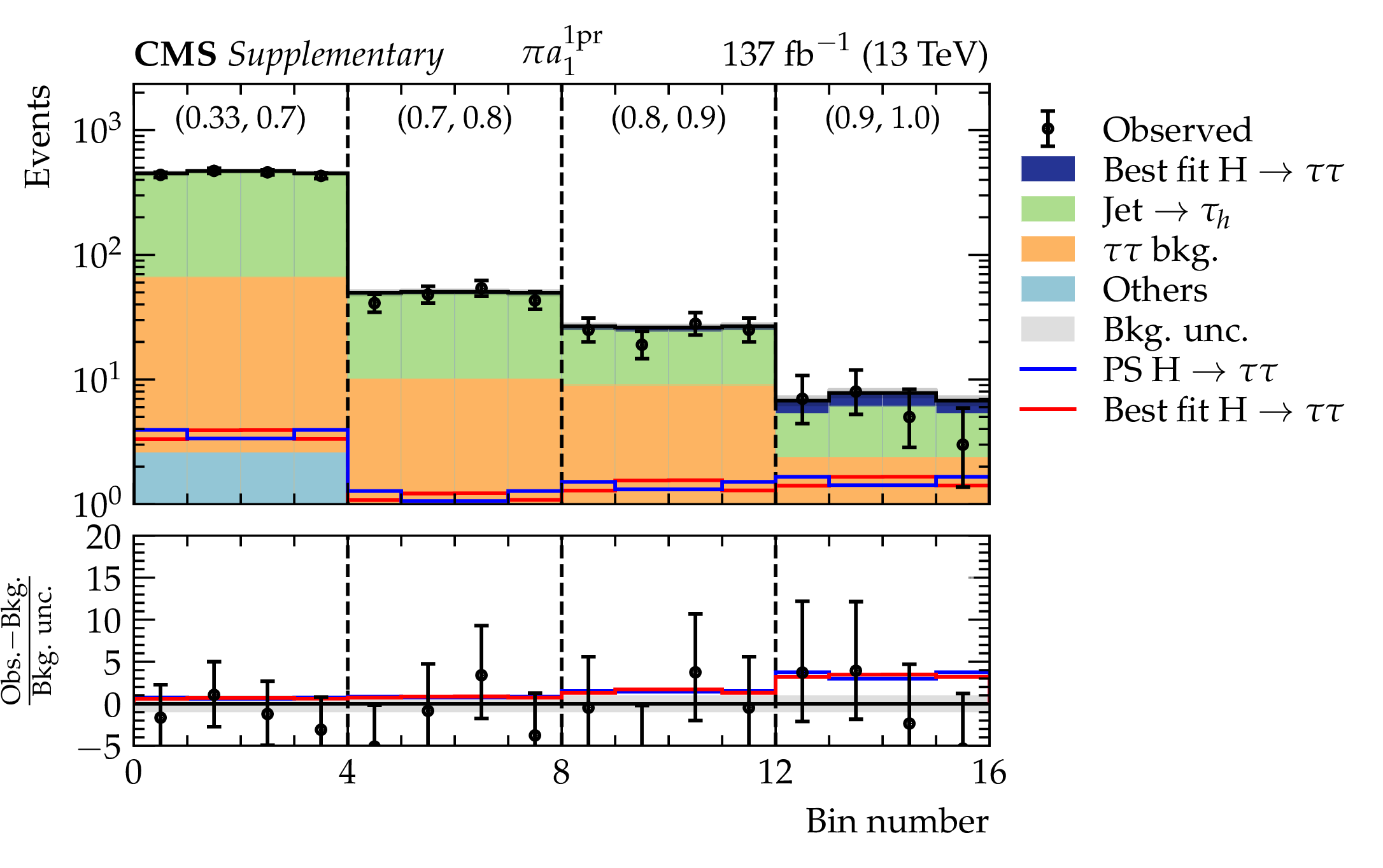
png pdf	Additional Figure 17: Distributions of $\phi _{\textit {CP}}$ in the $ {\pi}\mathrm {a_{1}^{1pr}}$ channel in windows of increasing MVA score, shown on top of each window. The best fit and pseudoscalar signal distributions are overlaid. The $x$ axis represents the cyclic bins in $\phi _{\textit {CP}}$ in the range of (0, 360$^{\circ}$). In the bottom plot the data minus the background template divided by the uncertainty in the background template is displayed, as well as the signal distributions divided by the uncertainty in the background template. The uncertainty band consists of the sum of the post-fit uncertainties in the background templates.
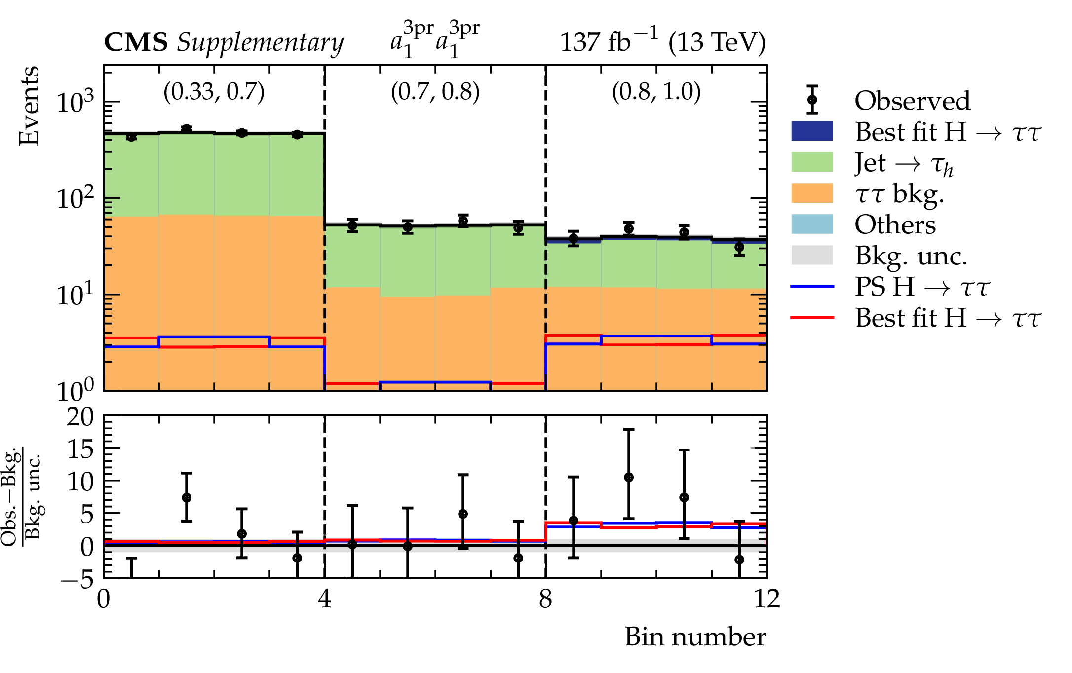
png pdf	Additional Figure 18: Distributions of $\phi _{\textit {CP}}$ in the $\mathrm {a_{1}^{3pr}}\mathrm {a_{1}^{3pr}}$ channel in windows of increasing MVA score, shown on top of each window. The polarimetric vector method was deployed to reconstruct $\phi _{\textit {CP}}$. The best fit and pseudoscalar signal distributions are overlaid. The $x$ axis represents the cyclic bins in $\phi _{\textit {CP}}$ in the range of (0, 360$^{\circ}$). In the bottom plot the data minus the background template divided by the uncertainty in the background template is displayed, as well as the signal distributions divided by the uncertainty in the background template. The uncertainty band consists of the sum of the post-fit uncertainties in the background templates.
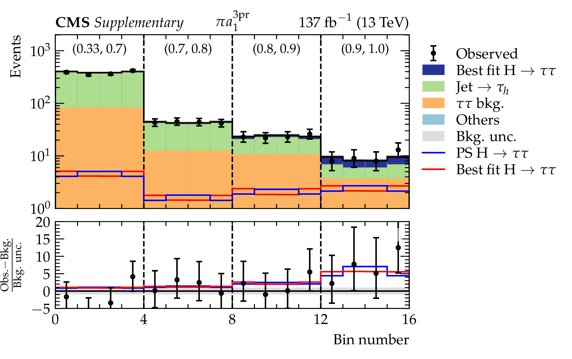
png pdf	Additional Figure 19: Distributions of $\phi _{\textit {CP}}$ in the $ {\pi}\mathrm {a_{1}^{3pr}}$ channel in windows of increasing MVA score, shown on top of each window. The best fit and pseudoscalar signal distributions are overlaid. The $x$ axis represents the cyclic bins in $\phi _{\textit {CP}}$ in the range of (0, 360$^{\circ}$). In the bottom plot the data minus the background template divided by the uncertainty in the background template is displayed, as well as the signal distributions divided by the uncertainty in the background template. The uncertainty band consists of the sum of the post-fit uncertainties in the background templates.
png pdf	Additional Figure 20: Distributions of $\phi _{\textit {CP}}$ in the $\mathrm {a_{1}^{3pr}} {\rho} $ channel in windows of increasing MVA score, shown on top of each window. The best fit and pseudoscalar signal distributions are overlaid. The $x$ axis represents the cyclic bins in $\phi _{\textit {CP}}$ in the range of (0, 360$^{\circ}$). In the bottom plot the data minus the background template divided by the uncertainty in the background template is displayed, as well as the signal distributions divided by the uncertainty in the background template. The uncertainty band consists of the sum of the post-fit uncertainties in the background templates.
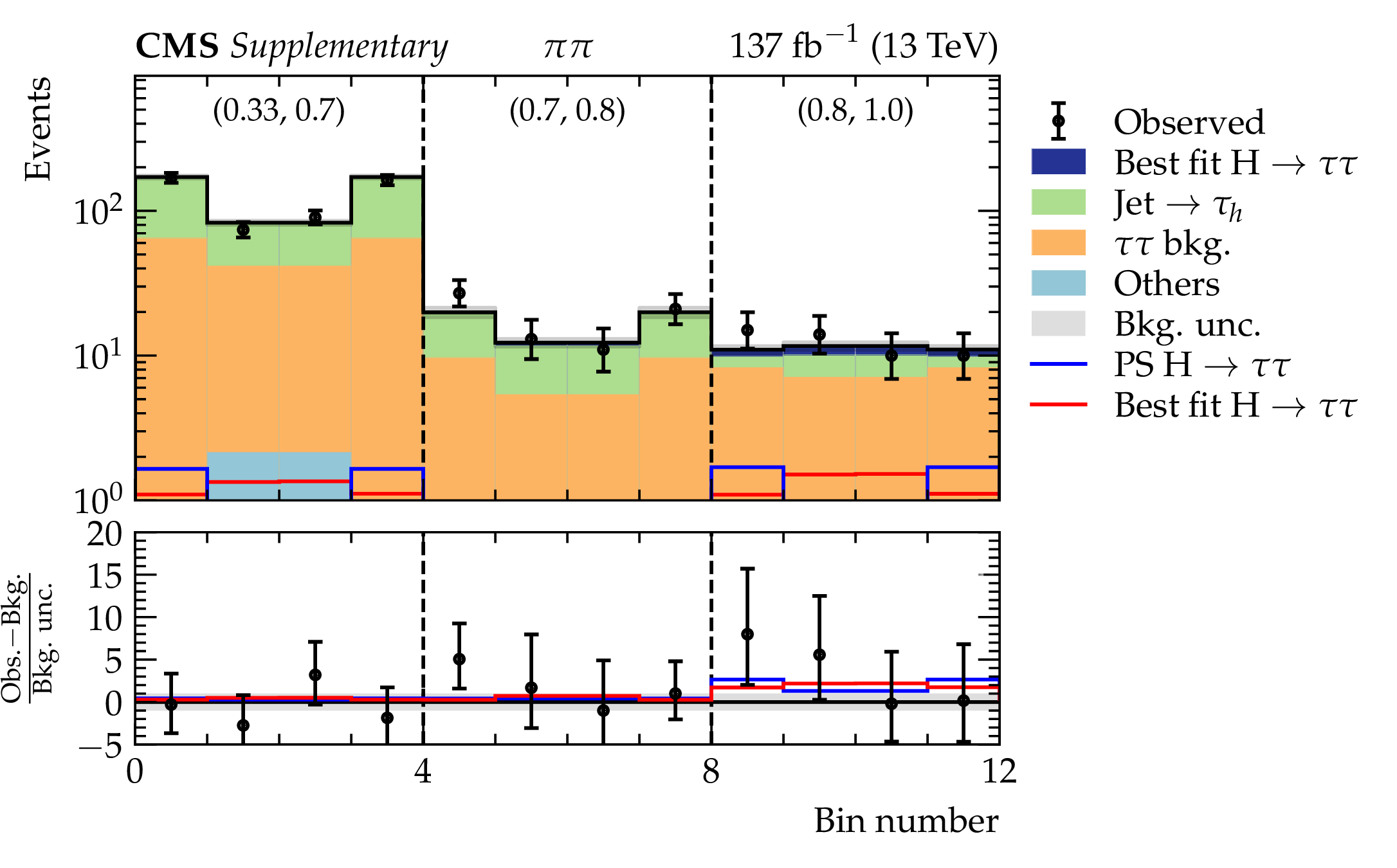
png pdf	Additional Figure 21: Distributions of $\phi _{\textit {CP}}$ in the $ {\pi} {\pi}$ channel in windows of increasing MVA score, shown on top of each window. The best fit and pseudoscalar signal distributions are overlaid. The $x$ axis represents the cyclic bins in $\phi _{\textit {CP}}$ in the range of (0, 360$^{\circ}$). In the bottom plot the data minus the background template divided by the uncertainty in the background template is displayed, as well as the signal distributions divided by the uncertainty in the background template. The uncertainty band consists of the sum of the post-fit uncertainties in the background templates.
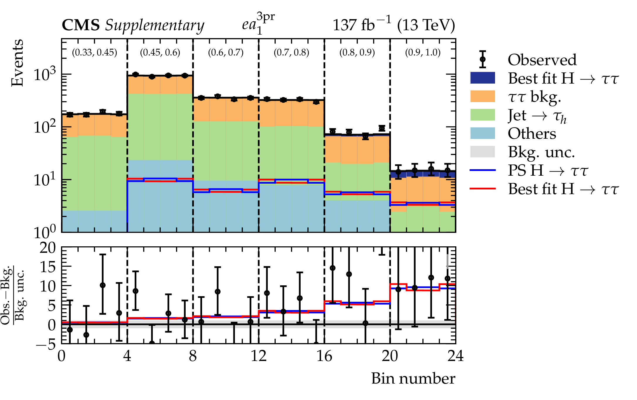
png pdf	Additional Figure 22: Distributions of $\phi _{\textit {CP}}$ in the $ {\mathrm {e}}\mathrm {a_{1}^{3pr}}$ channel in windows of increasing MVA score, shown on top of each window. The best fit and pseudoscalar signal distributions are overlaid. The $x$ axis represents the cyclic bins in $\phi _{\textit {CP}}$ in the range of (0, 360$^{\circ}$). In the bottom plot the data minus the background template divided by the uncertainty in the background template is displayed, as well as the signal distributions divided by the uncertainty in the background template. The uncertainty band consists of the sum of the post-fit uncertainties in the background templates.
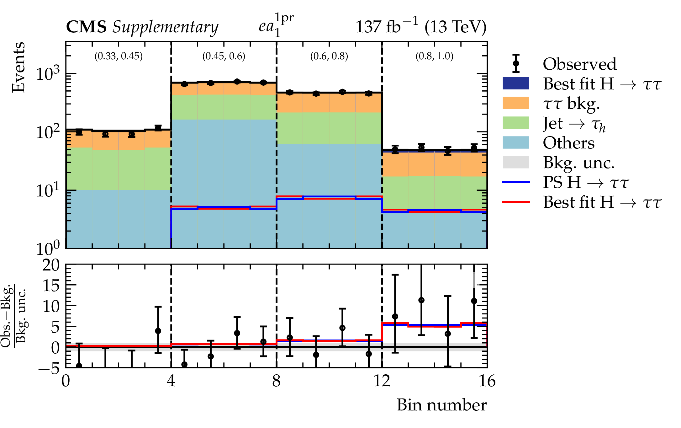
png pdf	Additional Figure 23: Distributions of $\phi _{\textit {CP}}$ in the $ {\mathrm {e}}\mathrm {a_{1}^{1pr}}$ channel in windows of increasing MVA score, shown on top of each window. The best fit and pseudoscalar signal distributions are overlaid. The $x$ axis represents the cyclic bins in $\phi _{\textit {CP}}$ in the range of (0, 360$^{\circ}$). In the bottom plot the data minus the background template divided by the uncertainty in the background template is displayed, as well as the signal distributions divided by the uncertainty in the background template. The uncertainty band consists of the sum of the post-fit uncertainties in the background templates.
png pdf	Additional Figure 24: A candidate event featuring a Higgs decaying into two ${\tau}$ leptons is depicted. The ${\tau}$ leptons decay into a muon (in red) and a $\mathrm {a_{1}}$ that decays in three charged pions (indicated by the orange cone and the calorimeter cells).
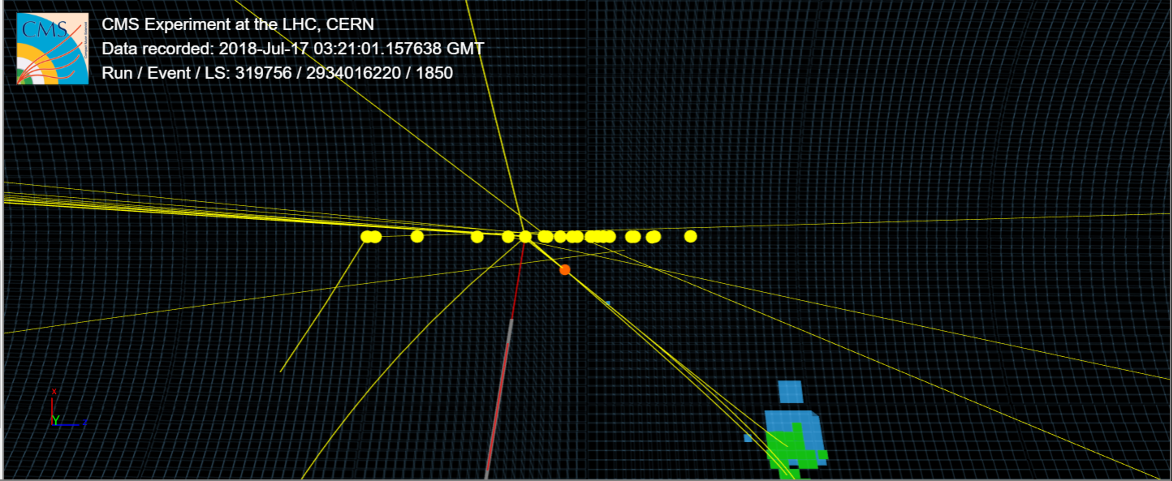
png pdf	Additional Figure 25: A zoomed view of a candidate event featuring a Higgs decaying into two ${\tau}$ leptons. The ${\tau}$ leptons decay into a muon (in red) and a $\mathrm {a_{1}}$ that decays into three charged pions. The displaced secondary vertex from which the tracks of the three charged pions candidates are emerging is indicated by the red circle. The pileup vertices are also indicated.
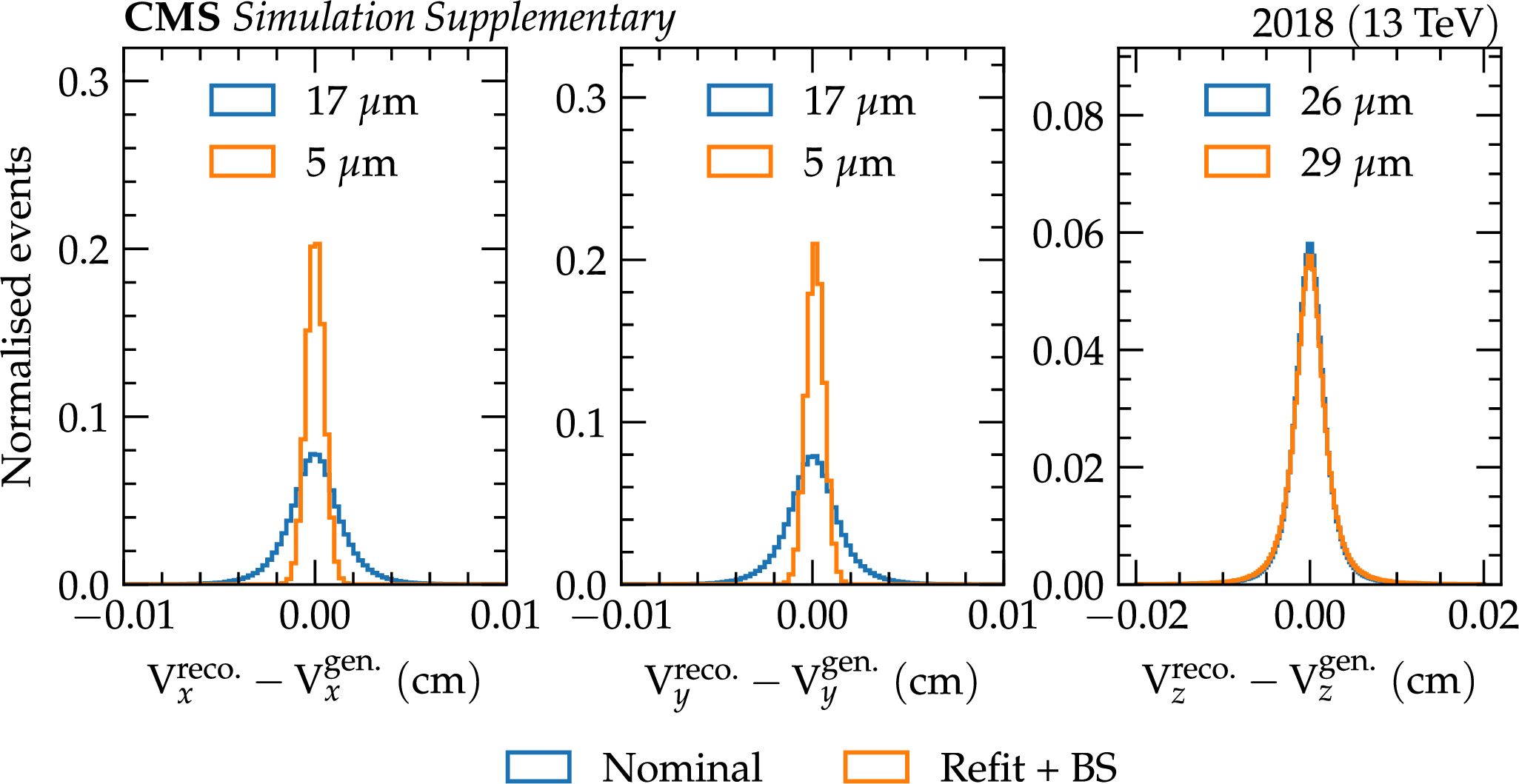
png pdf	Additional Figure 26: The resolution of the x (left), y (middle) and z (right) coordinate of the nominal primary vertex (blue), and the refitted beamspot-corrected primary vertex (red). The width of the distributions is indicated in the legend. Event samples were utilised in which a Higgs boson was produced in the gluon fusion and vector boson fusion process, and the samples were reweighed to their standard model cross section.
png pdf	Additional Figure 27: Expected negative log-likelihood scan for the combination of the $\tau _{{\mathrm {e}}}\tau _{\mathrm {h}}$, $\tau _{{{\mu}}}\tau _{\mathrm {h}}$ and $\tau _{\mathrm {h}}\tau _{\mathrm {h}}$ channels, including predictions for LHC Run 3 and Phase 2 integrated luminosities. The extrapolations have been made assuming systematic uncertainties as derived for the main analysis, while the statistical uncertainties were adjusted to different luminosity scenarios. The expected sensitivity to distinguish between the scalar and pseudo-scalar hypotheses, defined at $\alpha ^{{\mathrm {H}} \tau \tau} = $ 0 and $ \pm $ 90$ ^{\circ}$, respectively, exceeds 5 standard deviations for the Phase 2 scenario.
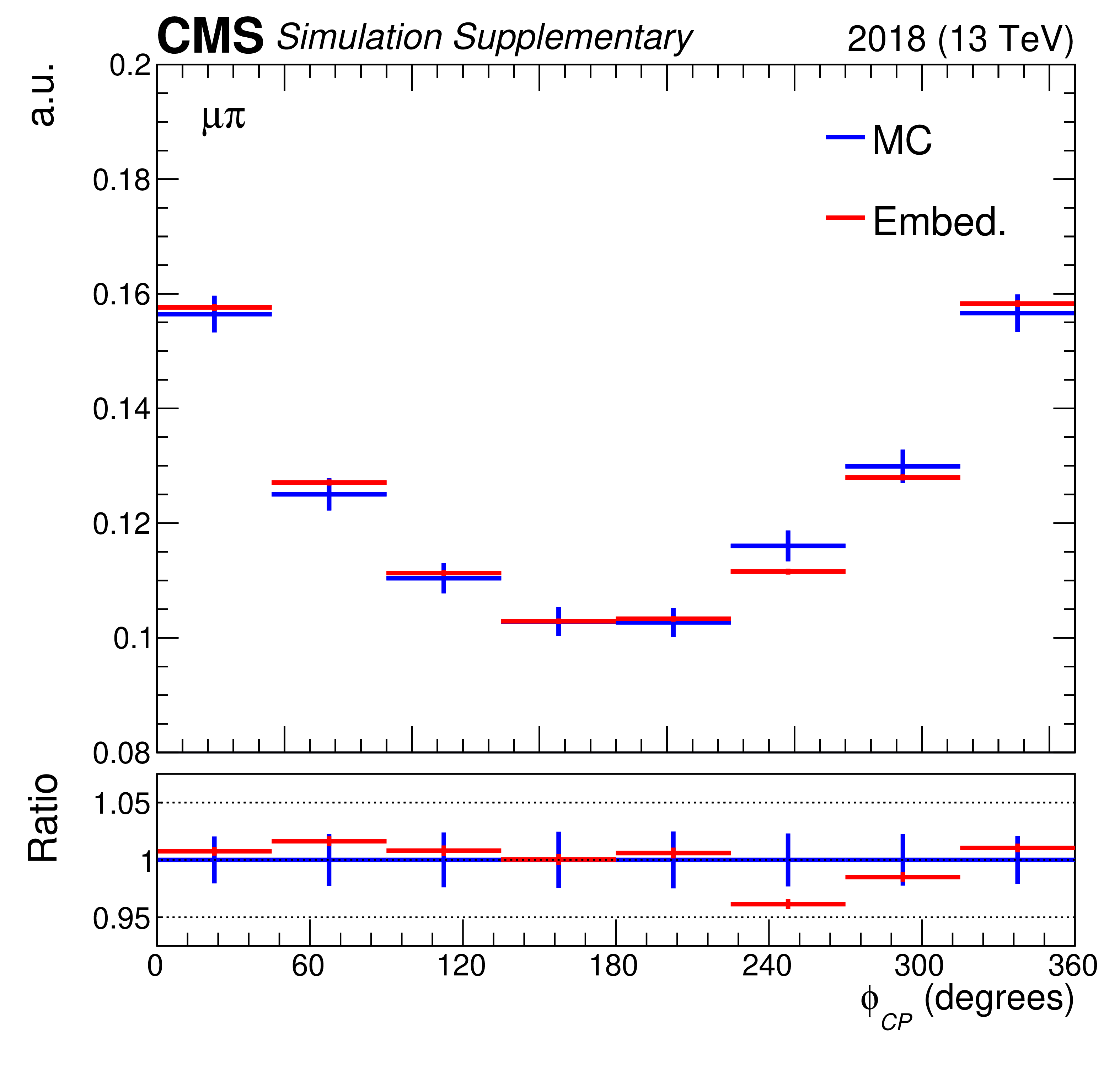
png pdf	Additional Figure 28: The ratio of $\phi _{\textit {CP}}$ for simulated events and events from the embedded samples in the $ {{\mu}} {\pi}$ final state are displayed. The shapes are consistent within statistical fluctuations.
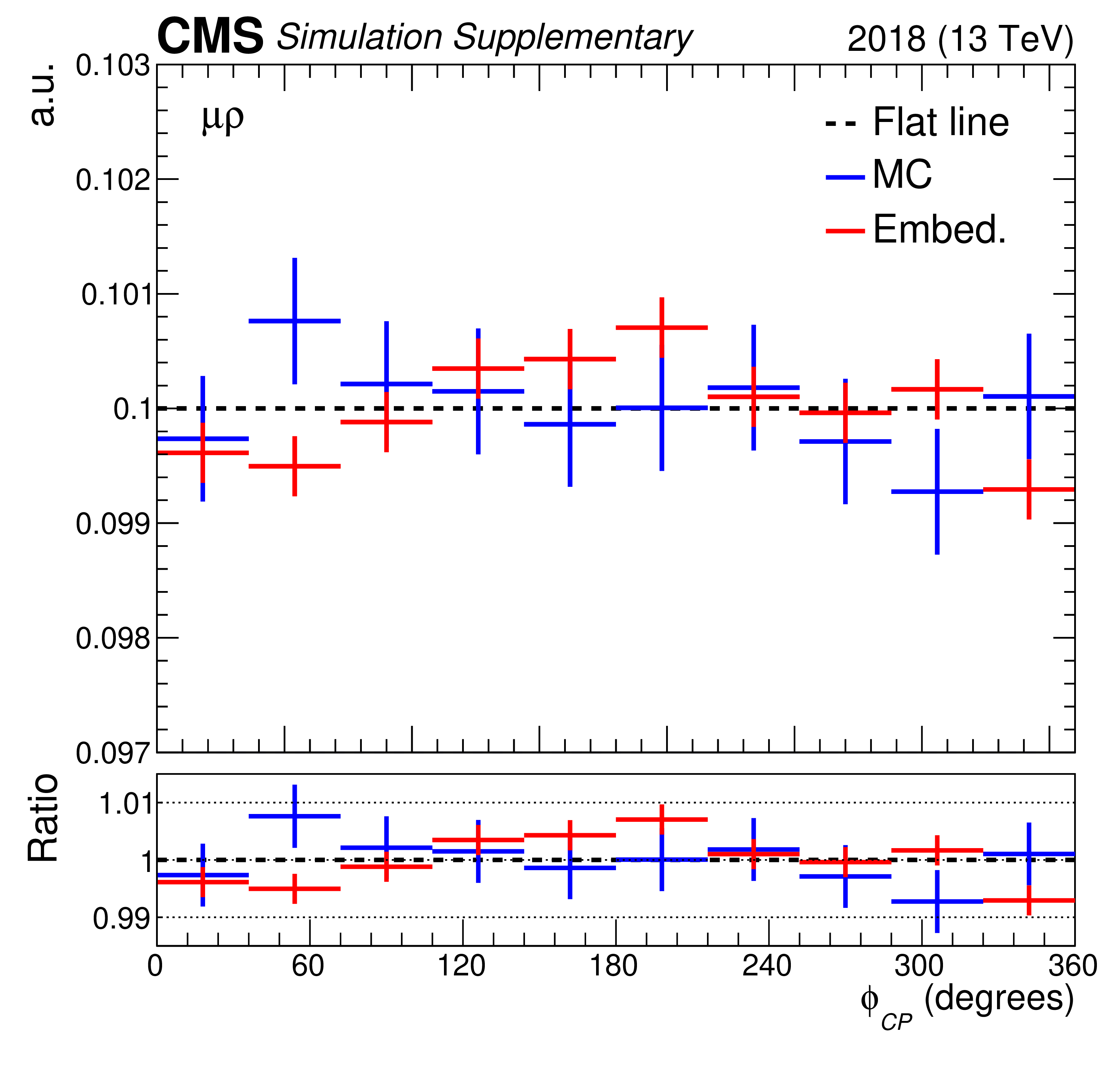
png pdf	Additional Figure 29: The ratio of $\phi _{\textit {CP}}$ for simulated events and events from the embedded samples in the $ {{\mu}} {\rho} $ final state are displayed. A minor residual effect is present in the embedded sample that is a consequence of misalignment effects in the embedding procedure. These effects cancel in the bin flattening procedure that is applied.
png pdf	Additional Figure 30: Observed correlations between $\alpha ^{{\mathrm {H}} \tau \tau}$ and the signal strength modifiers.
png pdf	Additional Figure 31: Two-dimensional scan of the $ {\mathrm {g}} {\mathrm {g}} {\mathrm {H}} $ signal strength modifier versus $\alpha ^{{\mathrm {H}} \tau \tau}$. The VBF+$ {\mathrm {H}} $ signal strength modifier is profiled.
png pdf	Additional Figure 32: Two-dimensional scan of the VBF+$ {\mathrm {H}} $ signal strength modifier versus $\alpha ^{{\mathrm {H}} \tau \tau}$. The $ {\mathrm {g}} {\mathrm {g}} {\mathrm {H}} $ signal strength modifier is profiled.
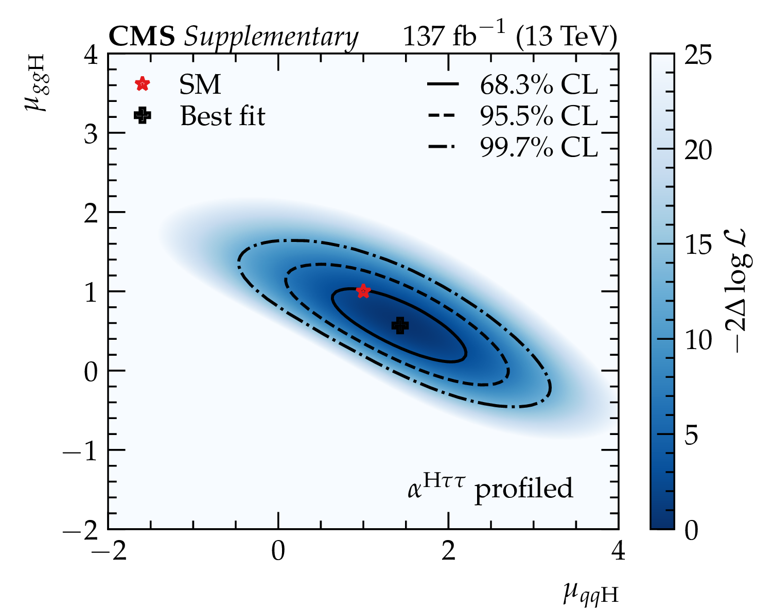
png pdf	Additional Figure 33: Two-dimensional scan of the $ {\mathrm {g}} {\mathrm {g}} {\mathrm {H}} $ and VBF+$ {\mathrm {H}} $ signal strength modifiers. The value of $\alpha ^{{\mathrm {H}} \tau \tau}$ is profiled.
png pdf	Additional Figure 34: Observed and expected distribution of the ${\pi ^{\pm}}$ energy from the $ {\tau}\rightarrow {\rho} \nu \rightarrow {\pi ^{\pm}} {\pi ^0}\nu $ decay chain in the $\tau _{{{\mu}}}\tau _{\mathrm {h}}$ channel, produced using the 2018 dataset prior to the fit used for the signal extraction. The invariant mass of the visible $ {\tau} {\tau}$ decay products is required to be smaller than 90 GeV in order to select a large fraction of $ {\mathrm {Z}} \rightarrow \tau \tau $ events. The uncertainty band includes statistical uncertainties and systematic uncertainties that affect the normalisation of the background distribution.
png pdf	Additional Figure 35: Observed and expected distribution of the ${\pi ^{\pm}}$ azimuthal angle $\phi $ from the $ {\tau}\rightarrow {\rho} \nu \rightarrow {\pi ^{\pm}} {\pi ^0}\nu $ decay chain in the $\tau _{{{\mu}}}\tau _{\mathrm {h}}$ channel, produced using the 2018 dataset prior to the fit used for the signal extraction. The invariant mass of the visible $ {\tau} {\tau}$ decay products is required to be smaller than 90 GeV in order to select a large fraction of $ {\mathrm {Z}} \rightarrow \tau \tau $ events. The uncertainty band includes statistical uncertainties and systematic uncertainties that affect the normalisation of the background distribution.
png pdf	Additional Figure 36: Observed and expected distribution of the ${\pi ^{\pm}}$ pseudorapidity $\eta $ from the $ {\tau}\rightarrow {\rho} \nu \rightarrow {\pi ^{\pm}} {\pi ^0}\nu $ decay chain in the $\tau _{{{\mu}}}\tau _{\mathrm {h}}$ channel, produced using the 2018 dataset prior to the fit used for the signal extraction. The invariant mass of the visible $ {\tau} {\tau}$ decay products is required to be smaller than 90 GeV in order to select a large fraction of $ {\mathrm {Z}} \rightarrow \tau \tau $ events. The uncertainty band includes statistical uncertainties and systematic uncertainties that affect the normalisation of the background distribution.
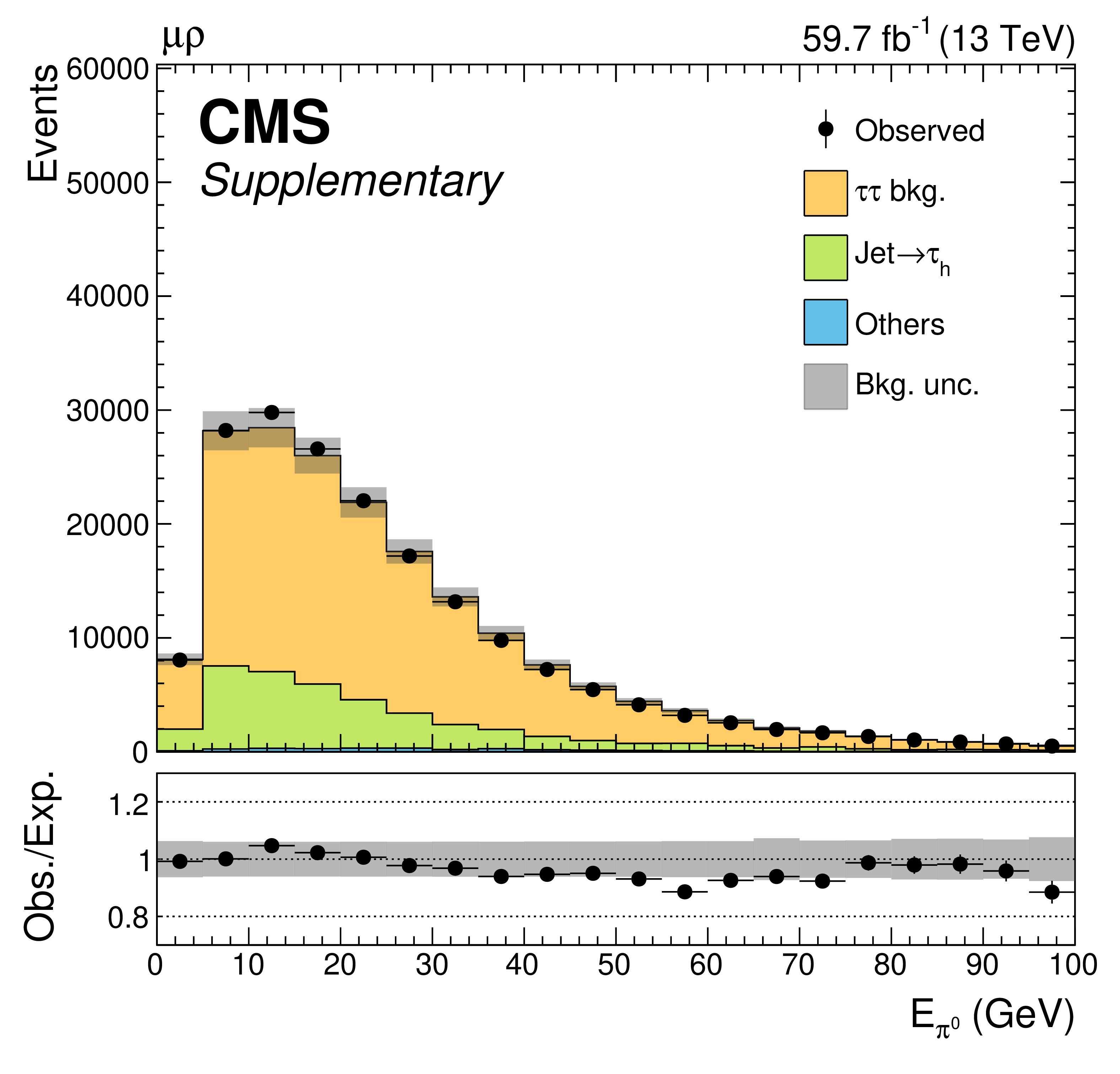
png pdf	Additional Figure 37: Observed and expected distribution of the ${\pi ^0}$ energy from the $ {\tau}\rightarrow {\rho} \nu \rightarrow {\pi ^{\pm}} {\pi ^0}\nu $ decay chain in the $\tau _{{{\mu}}}\tau _{\mathrm {h}}$ channel, produced using the 2018 dataset prior to the fit used for the signal extraction. The invariant mass of the visible $ {\tau} {\tau}$ decay products is required to be smaller than 90 GeV in order to select a large fraction of $ {\mathrm {Z}} \rightarrow \tau \tau $ events. The uncertainty band includes statistical uncertainties and systematic uncertainties that affect the normalisation of the background distribution.
png pdf	Additional Figure 38: Observed and expected distribution of the ${\pi ^0}$ azimuthal angle $\phi $ from the $ {\tau}\rightarrow {\rho} \nu \rightarrow {\pi ^{\pm}} {\pi ^0}\nu $ decay chain in the $\tau _{{{\mu}}}\tau _{\mathrm {h}}$ channel, produced using the 2018 dataset prior to the fit used for the signal extraction. The invariant mass of the visible $ {\tau} {\tau}$ decay products is required to be smaller than 90 GeV in order to select a large fraction of $ {\mathrm {Z}} \rightarrow \tau \tau $ events. The uncertainty band includes statistical uncertainties and systematic uncertainties that affect the normalisation of the background distribution.
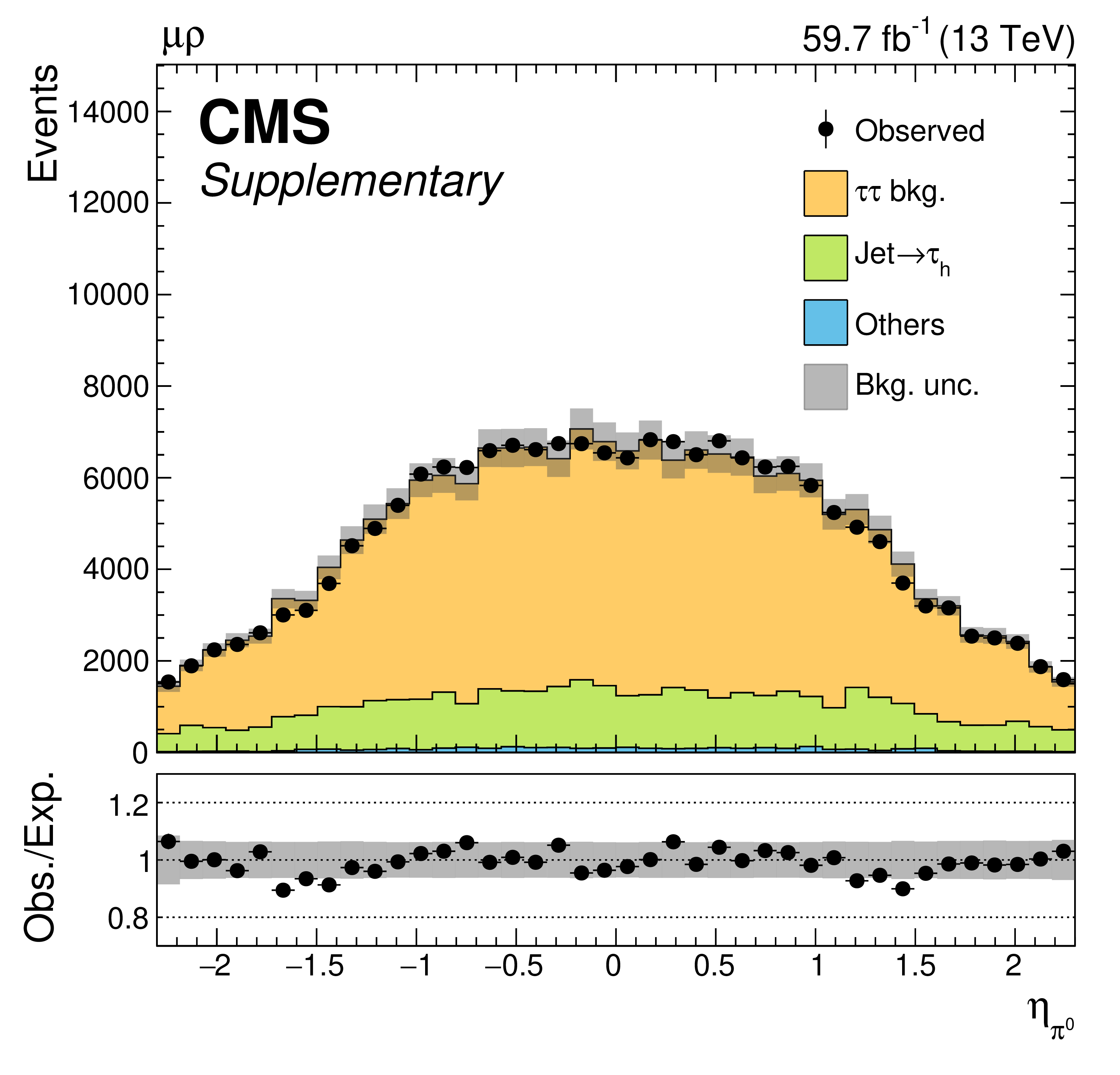
png pdf	Additional Figure 39: Observed and expected distribution of the ${\pi ^0}$ pseudorapidity $\eta $ from the $ {\tau}\rightarrow {\rho} \nu \rightarrow {\pi ^{\pm}} {\pi ^0}\nu $ decay chain in the $\tau _{{{\mu}}}\tau _{\mathrm {h}}$ channel, produced using the 2018 dataset prior to the fit used for the signal extraction. The invariant mass of the visible $ {\tau} {\tau}$ decay products is required to be smaller than 90 GeV in order to select a large fraction of $ {\mathrm {Z}} \rightarrow \tau \tau $ events. The uncertainty band includes statistical uncertainties and systematic uncertainties that affect the normalisation of the background distribution.
png pdf	Additional Figure 40: Observed and expected distribution of the ${\pi ^{\pm}}$ impact parameter ($\lambda $) magnitude from $ {\tau}\rightarrow {\pi ^{\pm}} \nu $ decays in the $\tau _{{{\mu}}}\tau _{\mathrm {h}}$ channel, produced using the 2018 dataset prior to the fit used for the signal extraction. The invariant mass of the visible $ {\tau} {\tau}$ decay products is required to be smaller than 90 GeV in order to select a large fraction of $ {\mathrm {Z}} \rightarrow \tau \tau $ events. The uncertainty band includes statistical uncertainties and systematic uncertainties that affect the normalisation of the background distribution.
png pdf	Additional Figure 41: Observed and expected distribution of the ${\pi ^{\pm}}$ impact parameter ($\lambda $) azimuthal angle $\phi $ from $ {\tau}\rightarrow {\pi ^{\pm}} \nu $ decays in the $\tau _{{{\mu}}}\tau _{\mathrm {h}}$ channel, produced using the 2018 dataset prior to the fit used for the signal extraction. The invariant mass of the visible $ {\tau} {\tau}$ decay products is required to be smaller than 90 GeV in order to select a large fraction of $ {\mathrm {Z}} \rightarrow \tau \tau $ events. The uncertainty band includes statistical uncertainties and systematic uncertainties that affect the normalisation of the background distribution.
png pdf	Additional Figure 42: Observed and expected distribution of the ${\pi ^{\pm}}$ impact parameter ($\lambda $) pseudorapidity $\eta $ from $ {\tau}\rightarrow {\pi ^{\pm}} \nu $ decays in the $\tau _{{{\mu}}}\tau _{\mathrm {h}}$ channel, produced using the 2018 dataset prior to the fit used for the signal extraction. The invariant mass of the visible $ {\tau} {\tau}$ decay products is required to be smaller than 90 GeV in order to select a large fraction of $ {\mathrm {Z}} \rightarrow \tau \tau $ events. The uncertainty band includes statistical uncertainties and systematic uncertainties that affect the normalisation of the background distribution.
png pdf	Additional Figure 43: Observed and expected distribution of the ${\tau}$ secondary vertex (SV) length relative to the primary vertex (PV) position from the $ {\tau}\rightarrow \mathrm {a_{1}}\nu \rightarrow {\pi ^{\pm}} {\pi^{\mp}} {\pi ^{\pm}} \nu $ decay chain in the $\tau _{{{\mu}}}\tau _{\mathrm {h}}$ channel, produced using the 2018 dataset prior to the fit used for the signal extraction. The invariant mass of the visible $ {\tau} {\tau}$ decay products is required to be smaller than 90 GeV in order to select a large fraction of $ {\mathrm {Z}} \rightarrow \tau \tau $ events. The uncertainty band includes statistical uncertainties and systematic uncertainties that affect the normalisation of the background distribution.
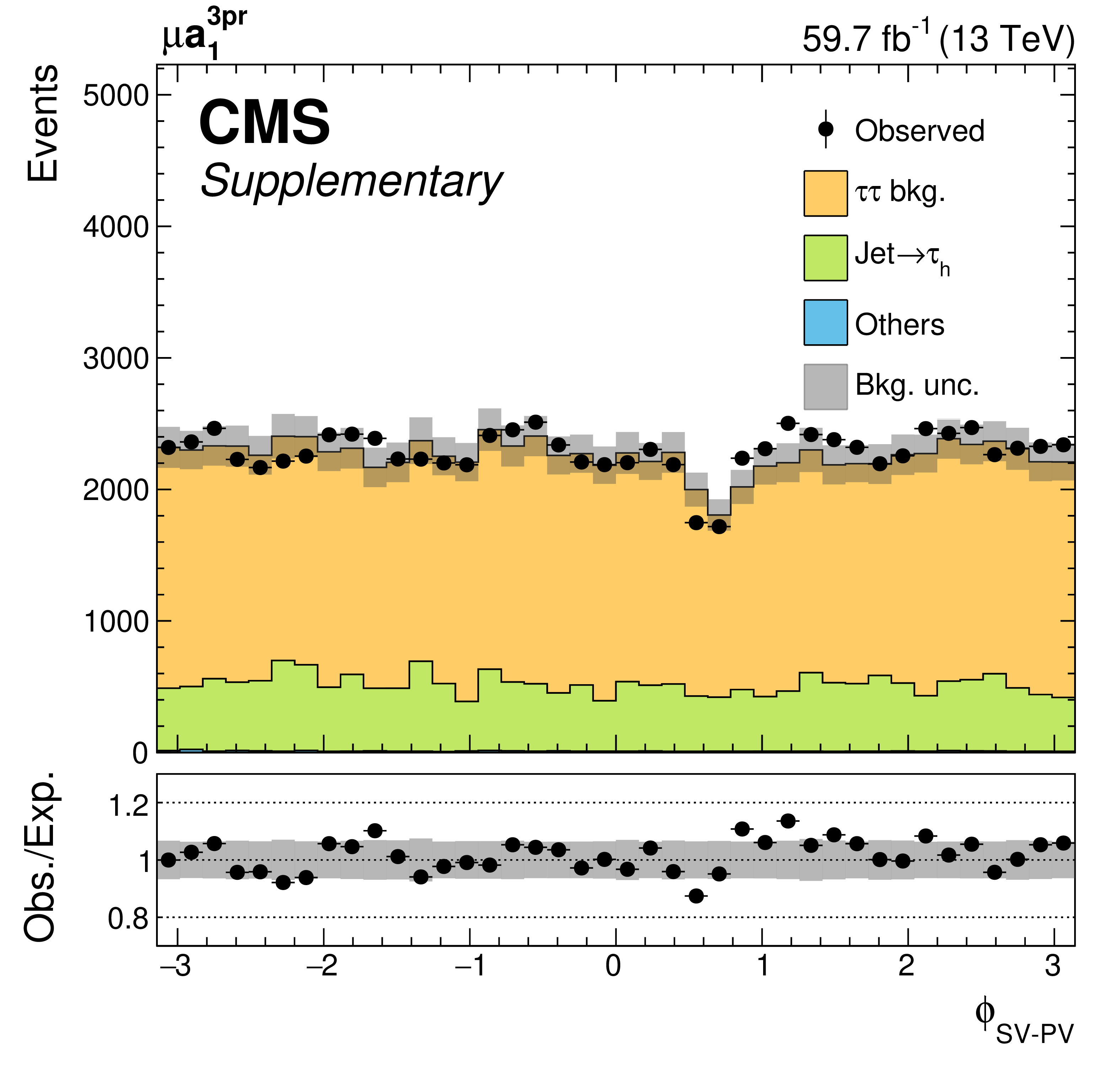
png pdf	Additional Figure 44: Observed and expected distribution of the ${\tau}$ secondary vertex (SV) azimuthal angle $\phi $ relative to the primary vertex (PV) position from the $ {\tau}\rightarrow \mathrm {a_{1}}\nu \rightarrow {\pi ^{\pm}} {\pi^{\mp}} {\pi ^{\pm}} \nu $ decay chain in the $\tau _{{{\mu}}}\tau _{\mathrm {h}}$ channel, produced using the 2018 dataset prior to the fit used for the signal extraction. The invariant mass of the visible $ {\tau} {\tau}$ decay products is required to be smaller than 90 GeV in order to select a large fraction of $ {\mathrm {Z}} \rightarrow \tau \tau $ events. The uncertainty band includes statistical uncertainties and systematic uncertainties that affect the normalisation of the background distribution.
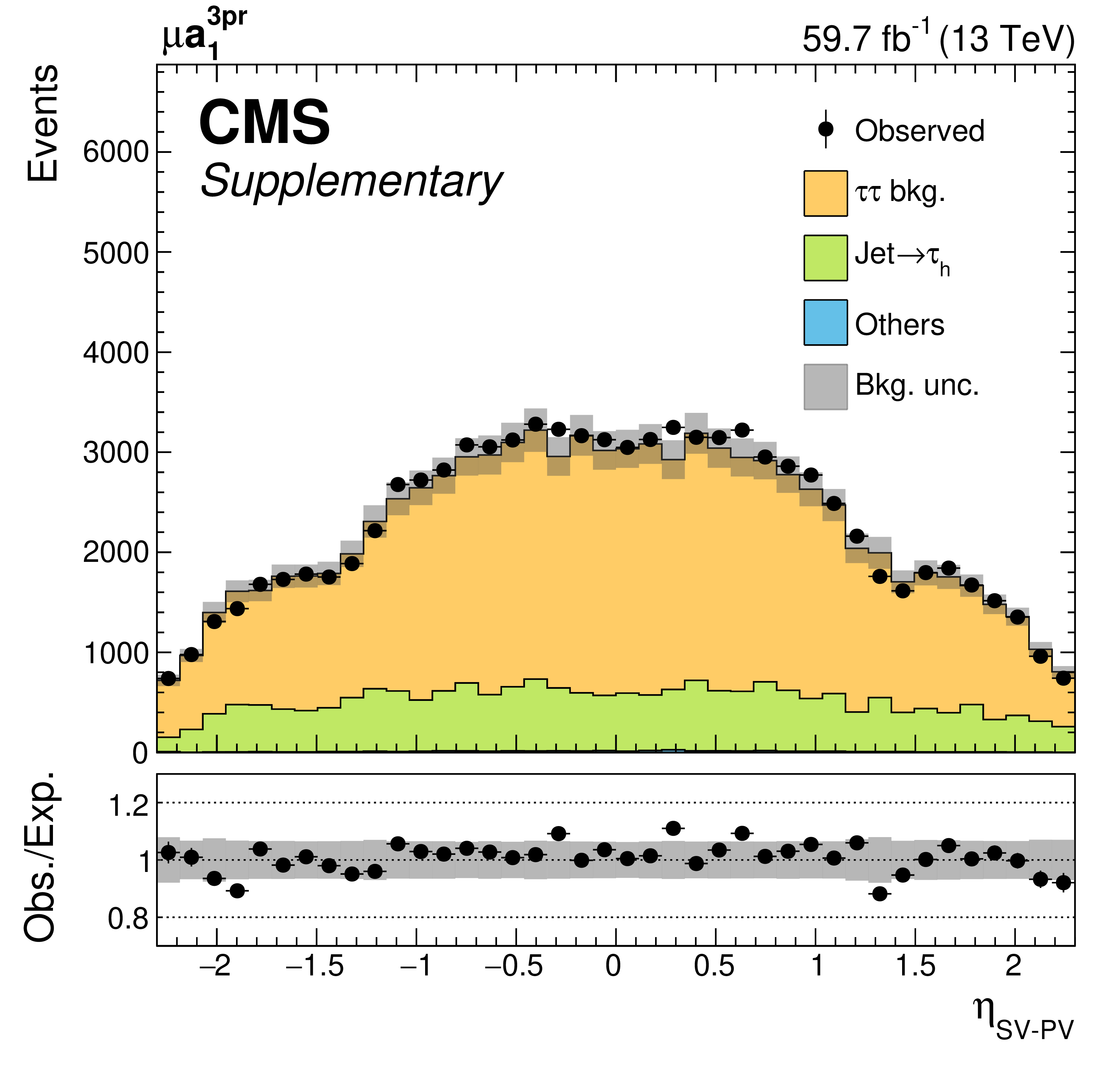
png pdf	Additional Figure 45: Observed and expected distribution of the ${\tau}$ secondary vertex (SV) pseudorapidity $\eta $ relative to the primary vertex (PV) position from the $ {\tau}\rightarrow \mathrm {a_{1}}\nu \rightarrow {\pi ^{\pm}} {\pi^{\mp}} {\pi ^{\pm}} \nu $ decay chain in the $\tau _{{{\mu}}}\tau _{\mathrm {h}}$ channel, produced using the 2018 dataset prior to the fit used for the signal extraction. The invariant mass of the visible $ {\tau} {\tau}$ decay products is required to be smaller than 90 GeV in order to select a large fraction of $ {\mathrm {Z}} \rightarrow \tau \tau $ events. The uncertainty band includes statistical uncertainties and systematic uncertainties that affect the normalisation of the background distribution.
png pdf	Additional Figure 46: Projections of the expected negative log-likelihood scans based on the Run 2 CMS analysis to an integrated luminosity, $\mathcal {L}$, of 3 ab$^{-1}$. The extrapolations have been made using different assumptions about the systematic uncertainties: no systematic uncertainties (red), assuming the same systematic uncertainties as for the Run 2 analysis (blue), systematic uncertainties scaled following the scheme used for the YR18 (arXiv:1902.00134) HL-LHC projections (black), and with "bin-by-bin" systematic uncertainties related to the finite statistics in the signal and background histograms scaled by 1/$\sqrt {\mathcal {L}}$ while all other systematic uncertainties are scaled following the YR18 scheme (magenta).
png pdf	Additional Figure 47: Projections of the expected negative log-likelihood scans based on the Run 2 CMS analysis to an integrated luminosity, $\mathcal {L}$, of 3 ab$^{-1}$. The extrapolations have been made using different assumptions about the systematic uncertainties: no systematic uncertainties (red), assuming the same systematic uncertainties as for the Run 2 analysis (blue), systematic uncertainties scaled following the scheme used for the YR18 (arXiv:1902.00134) HL-LHC projections (black), and with "bin-by-bin" systematic uncertainties related to the finite statistics in the signal and background histograms scaled by 1/$\sqrt {\mathcal {L}}$ while all other systematic uncertainties are scaled following the YR18 scheme (magenta). The range $|\alpha ^{{\mathrm {H}} \tau \tau}| < $ 40$^{\circ}$ is shown.

Additional Tables
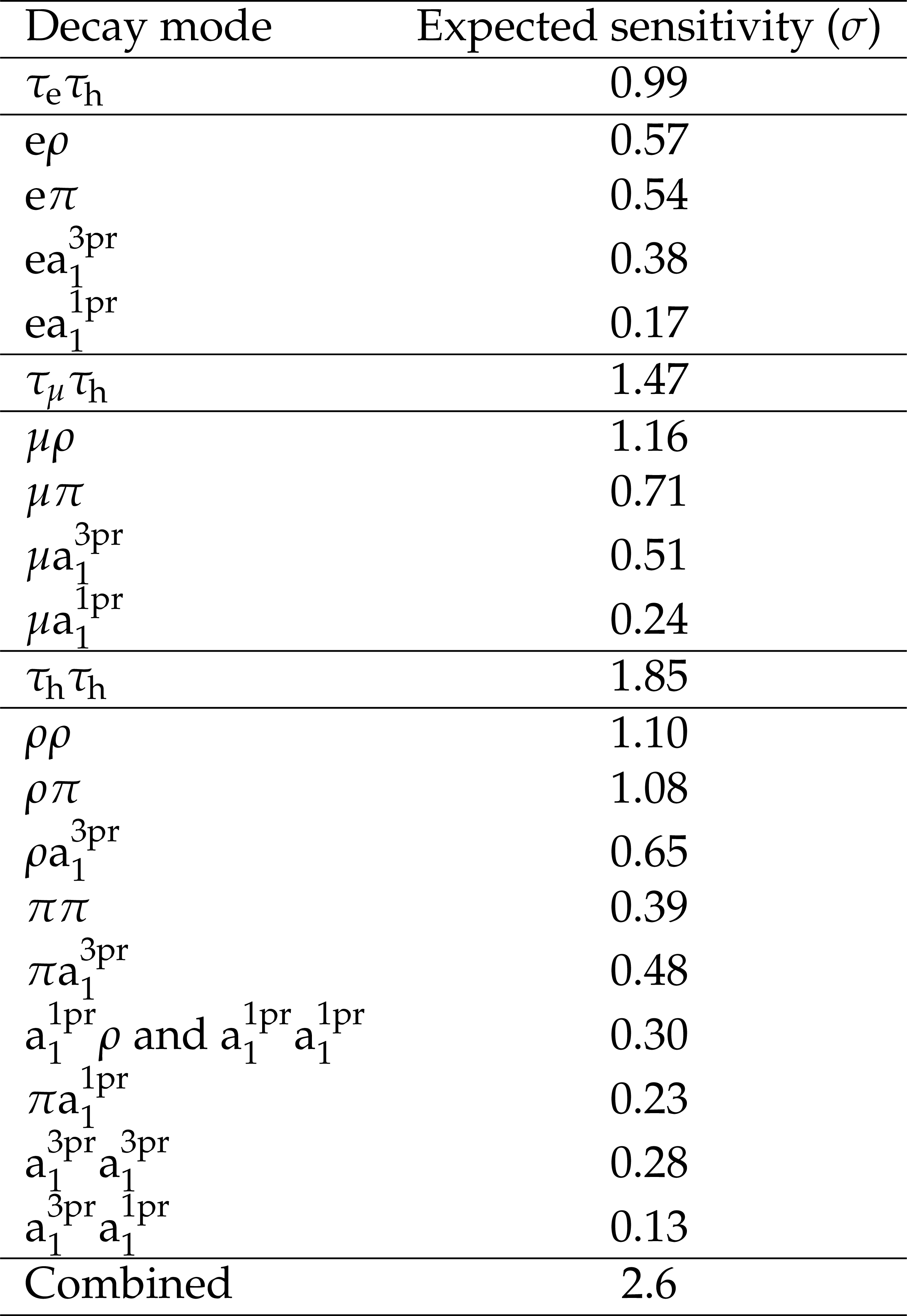
png pdf	Additional Table 1: The obtained expected sensitivities in standard deviations to distinguish between a CP-even and CP-odd $ {\mathrm {H}} {\tau} {\tau}$ coupling. Results are displayed for the individual decay modes (combined with their background categories), the combined $\tau _{{\mathrm {e}}}\tau _{\mathrm {h}}$, $\tau _{{{\mu}}}\tau _{\mathrm {h}}$ and $\tau _{\mathrm {h}}\tau _{\mathrm {h}}$ channels with their background categories, and the overall combination.
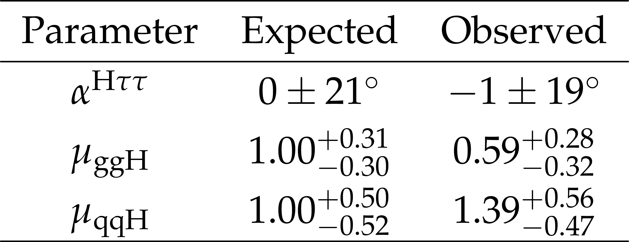
png pdf	Additional Table 2: The expected and observed values of $\alpha ^{{\mathrm {H}} \tau \tau}$ and the signal strength modifiers.

References
1	F. Englert and R. Brout	Broken symmetry and the mass of gauge vector mesons	PRL 13 (1964) 321
2	P. W. Higgs	Broken symmetries, massless particles and gauge fields	PL12 (1964) 132
3	P. W. Higgs	Broken symmetries and the masses of gauge bosons	PRL 13 (1964) 508
4	G. S. Guralnik, C. R. Hagen, and T. W. B. Kibble	Global conservation laws and massless particles	PRL 13 (1964) 585
5	P. W. Higgs	Spontaneous symmetry breakdown without massless bosons	PR145 (1966) 1156
6	T. W. B. Kibble	Symmetry breaking in non-abelian gauge theories	PR155 (1967) 1554
7	ATLAS Collaboration	Observation of a new particle in the search for the standard model Higgs boson with the ATLAS detector at the LHC	PLB 716 (2012) 1	1207.7214
8	CMS Collaboration	Observation of a new boson at a mass of 125 GeV with the CMS experiment at the LHC	PLB 716 (2012) 30	CMS-HIG-12-028 1207.7235
9	CMS Collaboration	Observation of a new boson with mass near 125 GeV in pp collisions at $ \sqrt{s} = $ 7 and 8 TeV	JHEP 06 (2013) 081	CMS-HIG-12-036 1303.4571
10	ATLAS and CMS Collaborations	Measurements of the Higgs boson production and decay rates and constraints on its couplings from a combined ATLAS and CMS analysis of the LHC pp collision data at $ \sqrt{s}= $ 7 and 8 TeV	JHEP 08 (2016) 045	1606.02266
11	CMS Collaboration	Observation of the Higgs boson decay to a pair of $ \tau $ leptons with the CMS detector	PLB 779 (2018) 283	CMS-HIG-16-043 1708.00373
12	ATLAS Collaboration	Cross-section measurements of the Higgs boson decaying into a pair of $ \tau $-leptons in proton-proton collisions at a centre-of-mass energy of 13 TeV with the ATLAS detector	PRD 99 (2019) 072001	1811.08856
13	CMS Collaboration	A measurement of the Higgs boson mass in the diphoton decay channel	PLB 805 (2020) 135425	CMS-HIG-19-004 2002.06398
14	CMS Collaboration	On the mass and spin-parity of the Higgs boson candidate via its decays to Z boson pairs	PRL 110 (2013) 081803	CMS-HIG-12-041 1212.6639
15	CMS Collaboration	Measurement of the properties of a Higgs boson in the four-lepton final state	PRD 89 (2014) 092007	CMS-HIG-13-002 1312.5353
16	CMS Collaboration	Constraints on the spin-parity and anomalous HVV couplings of the Higgs boson in proton collisions at 7 and 8 TeV	PRD 92 (2015) 012004	CMS-HIG-14-018 1411.3441
17	CMS Collaboration	Limits on the Higgs boson lifetime and width from its decay to four charged leptons	PRD 92 (2015) 072010	CMS-HIG-14-036 1507.06656
18	CMS Collaboration	Combined search for anomalous pseudoscalar HVV couplings in $ \mathrm{V}\mathrm{H}(\mathrm{H}\to \mathrm{b\bar{b}} $) production and $ \mathrm{H}\to\mathrm{V}\mathrm{V} $ decay	PLB 759 (2016) 672	CMS-HIG-14-035 1602.04305
19	CMS Collaboration	Constraints on anomalous Higgs boson couplings using production and decay information in the four-lepton final state	PLB 775 (2017) 1	CMS-HIG-17-011 1707.00541
20	CMS Collaboration	Constraints on anomalous HVV couplings from the production of Higgs bosons decaying to $ \tau $ lepton pairs	PRD 100 (2019) 112002	CMS-HIG-17-034 1903.06973
21	CMS Collaboration	Constraints on anomalous Higgs boson couplings to vector bosons and fermions in its production and decay using the four-lepton final state	PRD 104 (2021) 052004	CMS-HIG-19-009 2104.12152
22	ATLAS Collaboration	Evidence for the spin-0 nature of the Higgs boson using ATLAS data	PLB 726 (2013) 120	1307.1432
23	ATLAS Collaboration	Study of the spin and parity of the Higgs boson in diboson decays with the ATLAS detector	EPJC 75 (2015) 476	1506.05669
24	ATLAS Collaboration	Test of CP invariance in vector-boson fusion production of the Higgs boson using the optimal observable method in the ditau decay channel with the ATLAS detector	EPJC 76 (2016) 658	1602.04516
25	ATLAS Collaboration	Measurement of inclusive and differential cross sections in the $ \mathrm{H} \to \mathrm{Z}\mathrm{Z}^* \to 4\ell $ decay channel in pp collisions at $ \sqrt{s}= $ 13 TeV with the ATLAS detector	JHEP 10 (2017) 132	1708.02810
26	ATLAS Collaboration	Measurement of the Higgs boson coupling properties in the $ \mathrm{H} \to \mathrm{Z}\mathrm{Z}^* \to 4\ell $ decay channel at $ \sqrt{s} = $ 13 TeV with the ATLAS detector	JHEP 03 (2018) 095	1712.02304
27	ATLAS Collaboration	Measurements of Higgs boson properties in the diphoton decay channel with 36 fb$^{-1}$ of pp collision data at $ \sqrt{s} = $ 13 TeV with the ATLAS detector	PRD 98 (2018) 052005	1802.04146
28	C. Zhang and S. Willenbrock	Effective-field-theory approach to top-quark production and decay	PRD 83 (2011) 034006	1008.3869
29	R. Harnik et al.	Measuring CP violation in $ \mathrm{H} \to \tau^+ \tau^- $ at colliders	PRD 88 (2013) 076009	1308.1094
30	T. Ghosh, R. Godbole, and X. Tata	Determining the spacetime structure of bottom-quark couplings to spin-zero particles	PRD 100 (2019) 015026	1904.09895
31	A. V. Gritsan, R. Rontsch, M. Schulze, and M. Xiao	Constraining anomalous Higgs boson couplings to the heavy-flavor fermions using matrix element techniques	PRD 94 (2016) 055023	1606.03107
32	CMS Collaboration	Measurements of $ \mathrm{t\bar{t}}\mathrm{H} $ production and the CP structure of the Yukawa interaction between the Higgs boson and top quark in the diphoton decay channel	PRL 125 (2020) 061801	CMS-HIG-19-013 2003.10866
33	ATLAS Collaboration	CP properties of Higgs boson interactions with top quarks in the $ \mathrm{t\bar{t}}\mathrm{H} $ and $ \mathrm{t}\mathrm{H} $ processes using $ \mathrm{H} \to \gamma\gamma $ with the ATLAS detector	PRL 125 (2020) 061802	2004.04545
34	ATLAS Collaboration	Constraints on Higgs boson properties using $ \mathrm{W}\mathrm{W}^{*}(\rightarrow \mathrm{e}\nu\mu\nu) jj $ production in 36.1 fb$^{-1}$ of $ \sqrt{s} = $ 13 TeV pp collisions with the ATLAS detector	2021. Accepted by EPJC	2109.13808
35	D. Fontes, J. C. Romão, R. Santos, and J. P. Silva	Large pseudoscalar Yukawa couplings in the complex 2HDM	JHEP 06 (2015) 060	1502.01720
36	S. F. King, M. Muhlleitner, R. Nevzorov, and K. Walz	Exploring the CP-violating NMSSM: EDM constraints and phenomenology	NPB 901 (2015) 526	1508.03255
37	S. Berge, W. Bernreuther, and S. Kirchner	Determination of the Higgs CP-mixing angle in the tau decay channels at the LHC including the Drell--Yan background	EPJC 74 (2014) 3164	1408.0798
38	Particle Data Group, P. A. Zyla et al.	Review of particle physics	Prog. Theor. Exp. Phys. 2020 (2020) 083C01
39	S. Berge, W. Bernreuther, and S. Kirchner	Determination of the Higgs CP-mixing angle in the tau decay channels	Nucl. Part. Phys. Proc. 273-275 (2016) 841	1410.6362
40	S. Berge, W. Bernreuther, B. Niepelt, and H. Spiesberger	How to pin down the CP quantum numbers of a Higgs boson in its tau decays at the LHC	PRD 84 (2011) 116003	1108.0670
41	J. R. Dell'Aquila and C. A. Nelson	Distinguishing a spin-0 technipion and an elementary Higgs boson: $ {V}_{1} {V}_{2} $ modes with decays into $ \ell^-_{A} \boldsymbol{l}_{B} $ and/or $ q^-_{A} \boldsymbol{q}_{B} $	PRD 33 (1986) 93
42	M. Kramer, J. Kuhn, M. L. Stong, and P. M. Zerwas	Prospects of measuring the parity of Higgs particles	Z. Phys. C 64 (1994) 21	hep-ph/9404280
43	CMS Collaboration	Performance of the CMS Level-1 trigger in proton-proton collisions at $ \sqrt{s} = $ 13 TeV	JINST 15 (2020) P10017	CMS-TRG-17-001 2006.10165
44	CMS Collaboration	The CMS trigger system	JINST 12 (2017) P01020	CMS-TRG-12-001 1609.02366
45	CMS Collaboration	The CMS experiment at the CERN LHC	JINST 3 (2008) S08004	CMS-00-001
46	P. Nason	A new method for combining NLO QCD with shower Monte Carlo algorithms	JHEP 11 (2004) 040	hep-ph/0409146
47	S. Frixione, P. Nason, and C. Oleari	Matching NLO QCD computations with parton shower simulations: the POWHEG method	JHEP 11 (2007) 070	0709.2092
48	S. Alioli, P. Nason, C. Oleari, and E. Re	A general framework for implementing NLO calculations in shower Monte Carlo programs: the POWHEG BOX	JHEP 06 (2010) 043	1002.2581
49	E. Bagnaschi, G. Degrassi, P. Slavich, and A. Vicini	Higgs production via gluon fusion in the POWHEG approach in the SM and in the MSSM	JHEP 02 (2012) 088	1111.2854
50	P. Nason and C. Oleari	NLO Higgs boson production via vector-boson fusion matched with shower in POWHEG	JHEP 02 (2010) 037	0911.5299
51	T. Ježo and P. Nason	On the treatment of resonances in next-to-leading order calculations matched to a parton shower	JHEP 12 (2015) 065	1509.09071
52	F. Granata, J. M. Lindert, C. Oleari, and S. Pozzorini	NLO QCD+EW predictions for HV and HV+jet production including parton-shower effects	JHEP 09 (2017) 012	1706.03522
53	G. Klamke and D. Zeppenfeld	Higgs plus two jet production via gluon fusion as a signal at the CERN LHC	JHEP 04 (2007) 052	hep-ph/0703202
54	F. Demartin et al.	Higgs characterisation at NLO in QCD: CP properties of the top-quark Yukawa interaction	EPJC 74 (2014) 3065	1407.5089
55	K. Hamilton, P. Nason, E. Re, and G. Zanderighi	NNLOPS simulation of Higgs boson production	JHEP 10 (2013) 222	1309.0017
56	K. Hamilton, P. Nason, and G. Zanderighi	Finite quark-mass effects in the NNLOPS POWHEG+MiNLO Higgs generator	JHEP 05 (2015) 140	1501.04637
57	T. Sjostrand et al.	An introduction to PYTHIA 8.2	CPC 191 (2015) 159	1410.3012
58	T. Przedzinski, E. Richter-Was, and Z. Was	Documentation of TauSpinner algorithms: program for simulating spin effects in $ \tau $-lepton production at LHC	EPJC 79 (2019) 91	1802.05459
59	NNPDF Collaboration	Parton distributions for the LHC Run II	JHEP 04 (2015) 040	1410.8849
60	NNPDF Collaboration	Parton distributions from high-precision collider data	EPJC 77 (2017) 663	1706.00428
61	J. Alwall et al.	The automated computation of tree-level and next-to-leading order differential cross sections, and their matching to parton shower simulations	JHEP 07 (2014) 079	1405.0301
62	J. Alwall et al.	Comparative study of various algorithms for the merging of parton showers and matrix elements in hadronic collisions	EPJC 53 (2008) 473	0706.2569
63	S. Alioli, S.-O. Moch, and P. Uwer	Hadronic top-quark pair-production with one jet and parton showering	JHEP 01 (2012) 137	1110.5251
64	E. Re	Single-top Wt-channel production matched with parton showers using the POWHEG method	EPJC 71 (2011) 1547	1009.2450
65	R. Frederix, E. Re, and P. Torrielli	Single-top $ t $-channel hadroproduction in the four-flavour scheme with POWHEG and aMC@NLO	JHEP 09 (2012) 130	1207.5391
66	CMS Collaboration	Event generator tunes obtained from underlying event and multiparton scattering measurements	EPJC 76 (2016) 155	CMS-GEN-14-001 1512.00815
67	CMS Collaboration	Extraction and validation of a new set of CMS PYTHIA8 tunes from underlying-event measurements	EPJC 80 (2020) 4	CMS-GEN-17-001 1903.12179
68	GEANT4 Collaboration	GEANT4--a simulation toolkit	NIMA 506 (2003) 250
69	CMS Collaboration	Particle-flow reconstruction and global event description with the CMS detector	JINST 12 (2017) P10003	CMS-PRF-14-001 1706.04965
70	CMS Collaboration	Description and performance of track and primary-vertex reconstruction with the CMS tracker	JINST 9 (2014) P10009	CMS-TRK-11-001 1405.6569
71	K. Rose	Deterministic annealing for clustering, compression, classification, regression, and related optimization problems	Proc. IEEE 86 (1998) 2210
72	W. Waltenberger, R. Fruhwirth, and P. Vanlaer	Adaptive vertex fitting	JPG: Nuc. Part. Phys. 34 (2007) N343
73	M. Cacciari, G. P. Salam, and G. Soyez	The anti-$ {k_{\mathrm{T}}} $ jet clustering algorithm	JHEP 04 (2008) 063	0802.1189
74	CMS Collaboration	Performance of CMS muon reconstruction in pp collision events at $ \sqrt{s}= $ 7 TeV	JINST 7 (2012) P10002	CMS-MUO-10-004 1206.4071
75	CMS Collaboration	Performance of electron reconstruction and selection with the CMS detector in proton-proton collisions at $ \sqrt{s} = $ 8 TeV	JINST 10 (2015) P06005	CMS-EGM-13-001 1502.02701
76	M. Cacciari, G. P. Salam, and G. Soyez	FastJet user manual	EPJC 72 (2012) 1896	1111.6097
77	CMS Collaboration	Jet algorithms performance in 13 TeV data	CMS-PAS-JME-16-003	CMS-PAS-JME-16-003
78	CMS Collaboration	Jet energy scale and resolution in the CMS experiment in pp collisions at 8 TeV	JINST 12 (2017) P02014	CMS-JME-13-004 1607.03663
79	CMS Collaboration	Identification of heavy-flavour jets with the CMS detector in pp collisions at 13 TeV	JINST 13 (2018) P05011	CMS-BTV-16-002 1712.07158
80	D. Bertolini, P. Harris, M. Low, and N. Tran	Pileup per particle identification	JHEP 10 (2014) 059	1407.6013
81	CMS Collaboration	Performance of missing transverse momentum reconstruction in proton-proton collisions at $ \sqrt{s} = $ 13 TeV using the CMS detector	JINST 14 (2019) P07004	CMS-JME-17-001 1903.06078
82	CMS Collaboration	Performance of reconstruction and identification of $ \tau $ leptons decaying to hadrons and $ \nu_\tau $ in pp collisions at $ \sqrt{s}= $ 13 TeV	JINST 13 (2018) P10005	CMS-TAU-16-003 1809.02816
83	CMS Collaboration	Identification of hadronic tau lepton decays using a deep neural network	2022. Submitted to JINST	CMS-TAU-20-001 2201.08458
84	L. Bianchini, J. Conway, E. K. Friis, and C. Veelken	Reconstruction of the Higgs mass in $ \mathrm{H}\to\tau\tau $ events by dynamical likelihood techniques	J. Phys. Conf. Ser. 513 (2014) 022035
85	S. Berge and W. Bernreuther	Determining the CP parity of Higgs bosons at the LHC in the $ \tau $ to 1-prong decay channels	PLB 671 (2009) 470	0812.1910
86	S. Berge, W. Bernreuther, and S. Kirchner	Prospects of constraining the Higgs boson's CP nature in the tau decay channel at the LHC	PRD 92 (2015) 096012	1510.03850
87	G. R. Bower, T. Pierzchala, Z. Wças, and M. Worek	Measuring the Higgs boson's parity using $ \tau\to\rho\nu $	PLB 543 (2002) 227	hep-ph/0204292
88	V. Cherepanov, E. Richter-Was, and Z. Was	Monte Carlo, fitting and machine learning for tau leptons	SciPost Phys. Proc. 1 (2019) 018	1811.03969
89	V. Cherepanov and A. Zotz	Kinematic reconstruction of $ \mathrm{Z}/\mathrm{H} \to \tau\tau $ decay in proton-proton collisions	2018	1805.06988
90	S. Jadach, J. H. Kuhn, and Z. Wças	TAUOLA: A library of Monte Carlo programs to simulate decays of polarized $ \tau $ leptons	CPC 64 (1990) 275
91	M. Jezabek, Z. Wças, S. Jadach, and J. H. Kuhn	The $ \tau $ decay library TAUOLA, update with exact O(alpha) QED corrections in $ \tau\to\mu(\mathrm{e})\nu\bar{\nu} $ decay modes	CPC 70 (1992) 69
92	S. Jadach, Z. Wças, R. Decker, and J. H. Kuhn	The $ \tau $ decay library TAUOLA: Version 2.4	CPC 76 (1993) 361
93	CLEO Collaboration	Hadronic structure in the decay $ \tau\to\nu_{\tau}\pi^{\pm}\pi^{0}\pi^{0} $ and the sign of the $ \nu_{\tau} $ helicity	PRD 61 (2000) 012002	hep-ex/9902022
94	CMS Collaboration	Identification of hadronic tau decay channels using multivariate analysis (MVA decay mode)	CDS
95	T. Chen and C. Guestrin	XGBoost: A scalable tree boosting system	in Proceedings of the 22nd ACM SIGKDD International Conference on Knowledge Discovery and Data Mining, KDD '16, p. 785 2016	1603.02754
96	CMS Collaboration	An embedding technique to determine $ \tau\tau $ backgrounds in proton-proton collision data	JINST 14 (2019) P06032	CMS-TAU-18-001 1903.01216
97	CMS Collaboration	Measurement of the $ \mathrm{Z}/\gamma^{*} \to \tau\tau $ cross section in pp collisions at $ \sqrt{s} = $ 13 TeV and validation of $ \tau $ lepton analysis techniques	EPJC 78 (2018) 708	CMS-HIG-15-007 1801.03535
98	CMS Collaboration	Measurements of inclusive W and Z cross sections in pp collisions at $ \sqrt {s} = $ 7 TeV	JHEP 01 (2011) 080	CMS-EWK-10-002 1012.2466
99	CMS Collaboration	Measurement of the differential cross section for top quark pair production in pp collisions at $ \sqrt{s} = $ 8 TeV	EPJC 75 (2015) 2339	CMS-TOP-12-028 1505.04480
100	LHC Higgs Cross Section Working Group	Handbook of LHC Higgs cross sections: 4. deciphering the nature of the Higgs sector	CERN (2016)	1610.07922
101	CMS Collaboration	CMS luminosity measurements for the 2016 data-taking period	CMS-PAS-LUM-17-001	CMS-PAS-LUM-17-001
102	CMS Collaboration	CMS luminosity measurement for the 2017 data-taking period at $ \sqrt{s} = $ 13 TeV	CMS-PAS-LUM-17-004	CMS-PAS-LUM-17-004
103	CMS Collaboration	CMS luminosity measurement for the 2018 data-taking period at $ \sqrt{s} = $ 13 TeV	CMS-PAS-LUM-18-002	CMS-PAS-LUM-18-002
104	Y. Li and F. Petriello	Combining QCD and electroweak corrections to dilepton production in the framework of the FEWZ simulation code	PRD 86 (2012) 094034	1208.5967
105	M. Czakon and A. Mitov	Top++: A program for the calculation of the top-pair cross-section at hadron colliders	CPC 185 (2014) 2930	1112.5675
106	CMS Collaboration	Measurement of the WZ production cross section in pp collisions at $ \sqrt{s}= $ 13 TeV	PLB 766 (2017) 268	CMS-SMP-16-002 1607.06943
107	CMS Collaboration	Cross section measurement of $ t $-channel single top quark production in pp collisions at $ \sqrt s = $ 13 TeV	PLB 772 (2017) 752	CMS-TOP-16-003 1610.00678
108	R. Barlow and C. Beeston	Fitting using finite Monte Carlo samples	CPC 77 (1993) 219
109	J. S. Conway	Incorporating nuisance parameters in likelihoods for multisource spectra	in PHYSTAT 2011, p. 115 2011	1103.0354
110	ATLAS and CMS Collaborations, and LHC Higgs Combination Group	Procedure for the LHC Higgs boson search combination in Summer 2011	CMS-NOTE-2011-005
111	CMS Collaboration	Precise determination of the mass of the Higgs boson and tests of compatibility of its couplings with the standard model predictions using proton collisions at 7 and 8 TeV	EPJC 75 (2015) 212	CMS-HIG-14-009 1412.8662
112	CMS Collaboration	HEPData record for this analysis	link

Compact Muon Solenoid LHC, CERN

© Copyright CERN 2018 for the benefit of the CMS Collaboration