

Compact Muon Solenoid
LHC, CERN
| CMS-SUS-19-010 ; CERN-EP-2021-022 | ||
| Search for top squark production in fully-hadronic final states in proton-proton collisions at $\sqrt{s} = $ 13 TeV | ||
| CMS Collaboration | ||
| 1 March 2021 | ||
| Phys. Rev. D 104 (2021) 052001 | ||
| Abstract: A search for production of the supersymmetric partners of the top quark, top squarks, is presented. The search is based on proton-proton collision events containing multiple jets, no leptons, and large transverse momentum imbalance. The data were collected with the CMS detector at the CERN LHC at a center-of-mass energy of 13 TeV, and correspond to an integrated luminosity of 137 fb$^{-1}$. The targeted signal production scenarios are direct and gluino-mediated top squark production, including scenarios in which the top squark and neutralino masses are nearly degenerate. The search utilizes novel algorithms based on deep neural networks that identify hadronically decaying top quarks and W bosons, which are expected in many of the targeted signal models. No statistically significant excess of events is observed relative to the expectation from the standard model, and limits on the top squark production cross section are obtained in the context of simplified supersymmetric models for various production and decay modes. Exclusion limits as high as 1310 GeV are established at the 95% confidence level on the mass of the top squark for direct top squark production models, and as high as 2260 GeV on the mass of the gluino for gluino-mediated top squark production models. These results represent a significant improvement over the results of previous searches for supersymmetry by CMS in the same final state. | ||
| Links: e-print arXiv:2103.01290 [hep-ex] (PDF) ; CDS record ; inSPIRE record ; HepData record ; CADI line (restricted) ; | ||
| Figures & Tables | Summary | Additional Figures & Tables | References | CMS Publications |
|---|
|
Additional information on efficiencies needed for reinterpretation of
these results are available here Additional technical material for CMS speakers can be found here |
| Figures | |
png pdf |
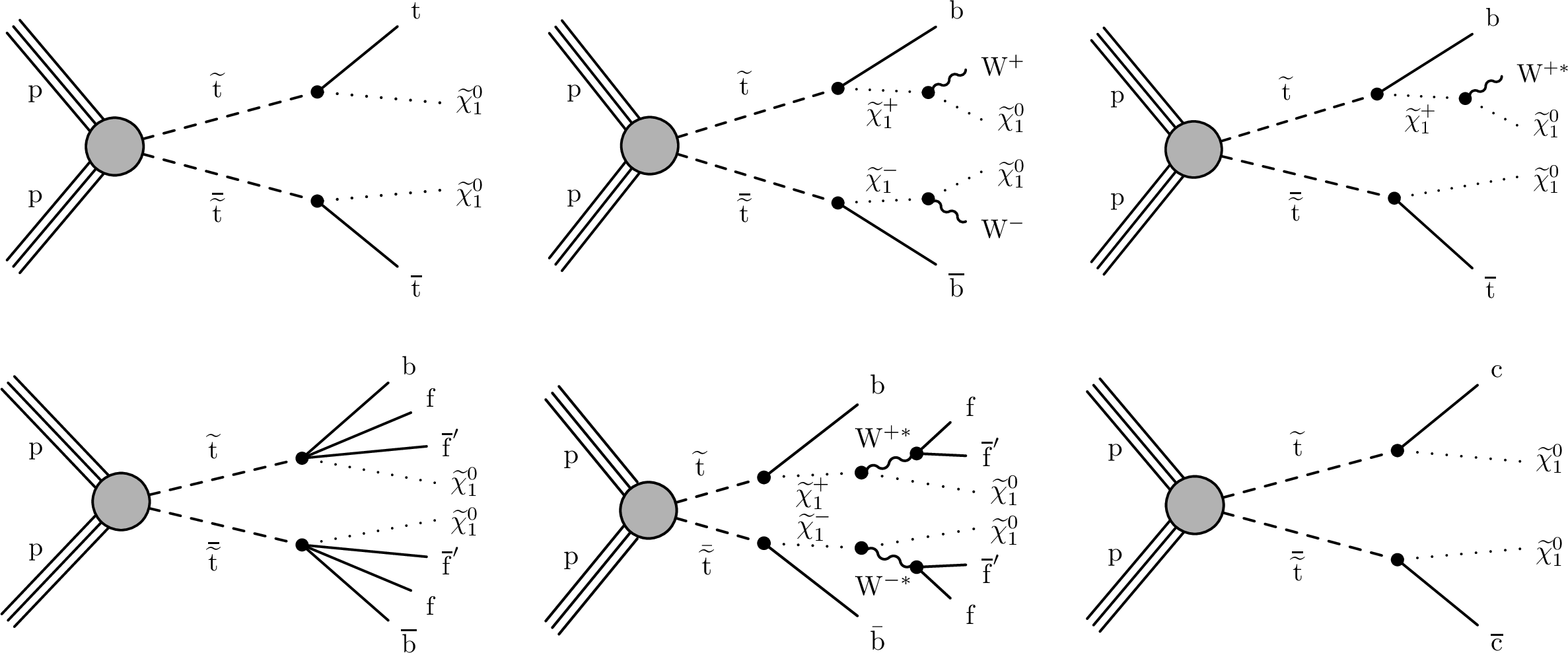
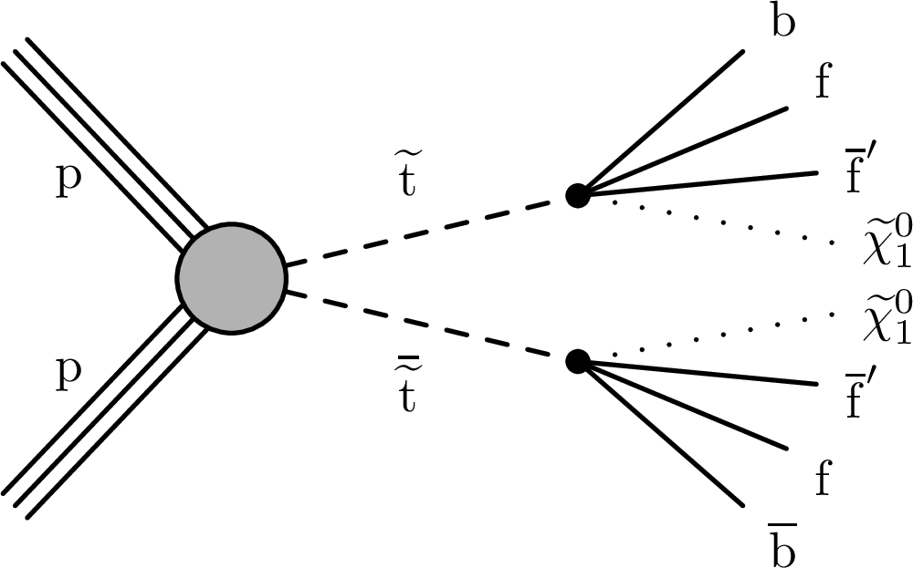
Figure 1:
Diagrams for the direct top squark production scenarios considered in this study: the T2tt (upper left), T2bW (upper middle), T2tb (upper right), T2ttC (lower left), T2bWC (lower middle), and T2cc (lower right) simplified models. |
png pdf |
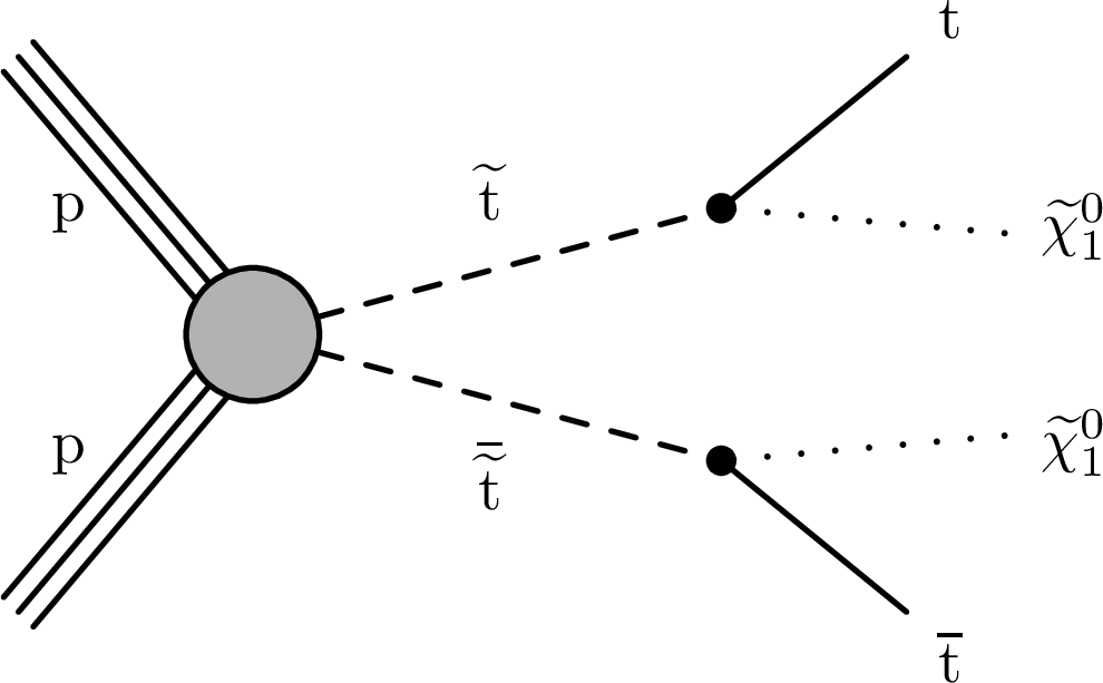
Figure 1-a:
Diagram for the direct top squark production in the T2tt simplified model. |
png pdf |
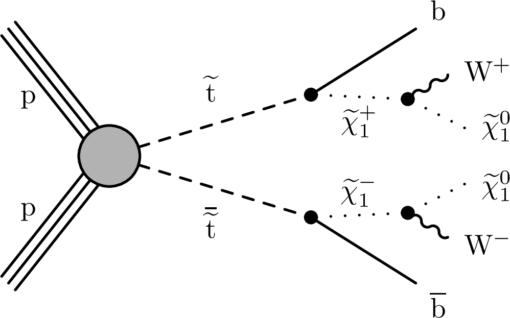
Figure 1-b:
Diagram for the direct top squark production in the T2bW simplified model. |
png pdf |
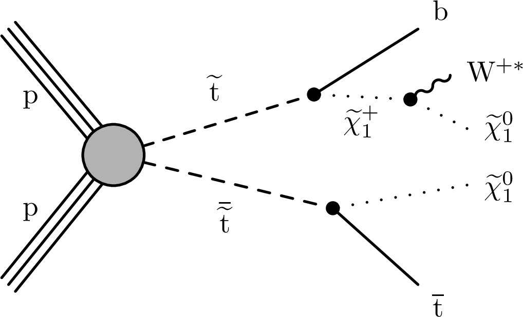
Figure 1-c:
Diagram for the direct top squark production in the T2tb simplified model. |
png pdf |
Figure 1-d:
Diagram for the direct top squark production in the T2ttC simplified model. |
png pdf |
Figure 1-e:
Diagram for the direct top squark production in the T2bWC simplified model. |

png pdf |
Figure 1-f:
Diagram for the direct top squark production in the T2cc simplified model. |
png pdf |
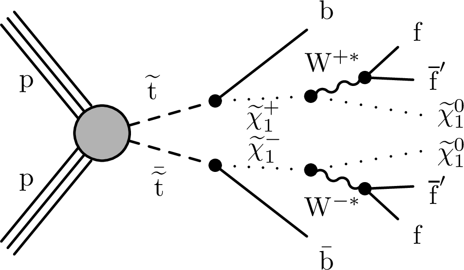
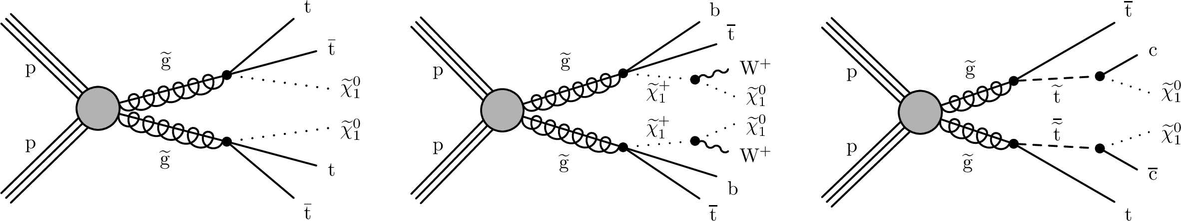
Figure 2:
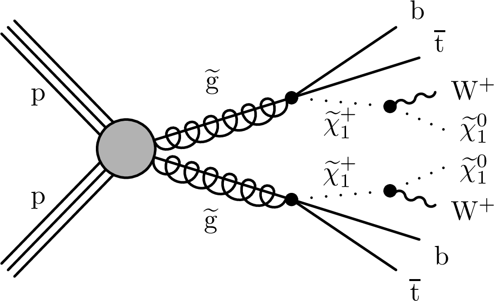
Diagrams for the direct gluino production scenarios considered in this study: the T1tttt (left), T1ttbb (middle), and T5ttcc (right) simplified models. |
png pdf |
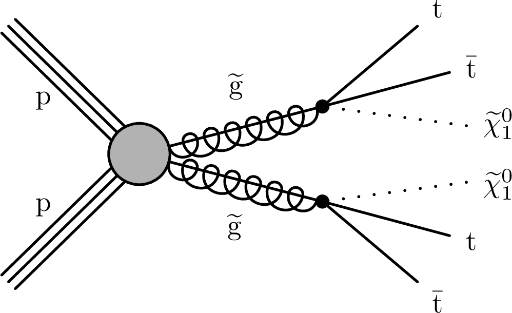
Figure 2-a:
Diagram for the direct gluino production in the T1tttt simplified model. |
png pdf |
Figure 2-b:
Diagram for the direct gluino production in the T1ttbb simplified model. |
png pdf |
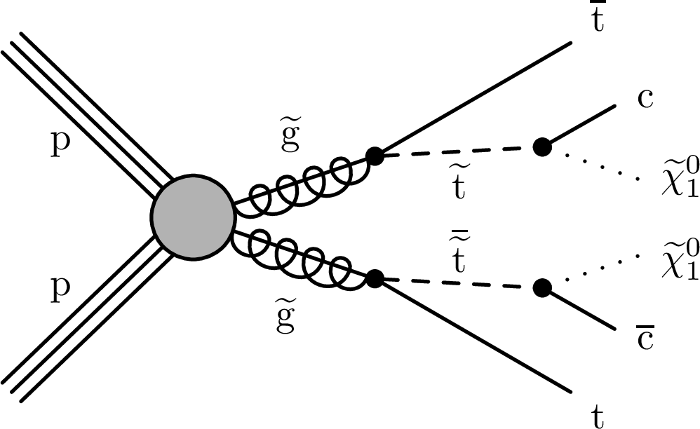
Figure 2-c:
Diagram for the direct gluino production in the T5ttcc simplified model. |
png pdf |
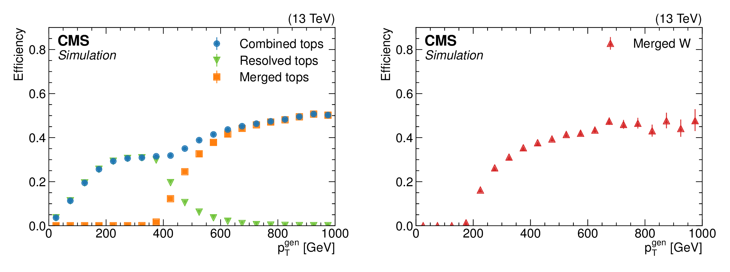
Figure 3:
Top quark and W boson tagging efficiencies are shown as a function of the generator-level top quark ${p_{\mathrm {T}}}$ and the generator-level W boson ${p_{\mathrm {T}}}$, respectively, for the merged tagging algorithm and resolved tagging algorithm described in Section 5.2. The left plot shows the efficiencies as calculated in a sample of simulated ${\mathrm{t} {}\mathrm{\bar{t}}}$ events in which one top quark decays leptonically, while the other decays hadronically. The right plot shows the W boson tagging efficiency when calculated in a sample of simulated WW events. In addition to the individual algorithms shown as orange squares (boosted top quarks), green inverted triangles (resolved top quarks), and red triangles (boosted W bosons), the total top quark tagging efficiency (blue dots) is also shown. |
png pdf |
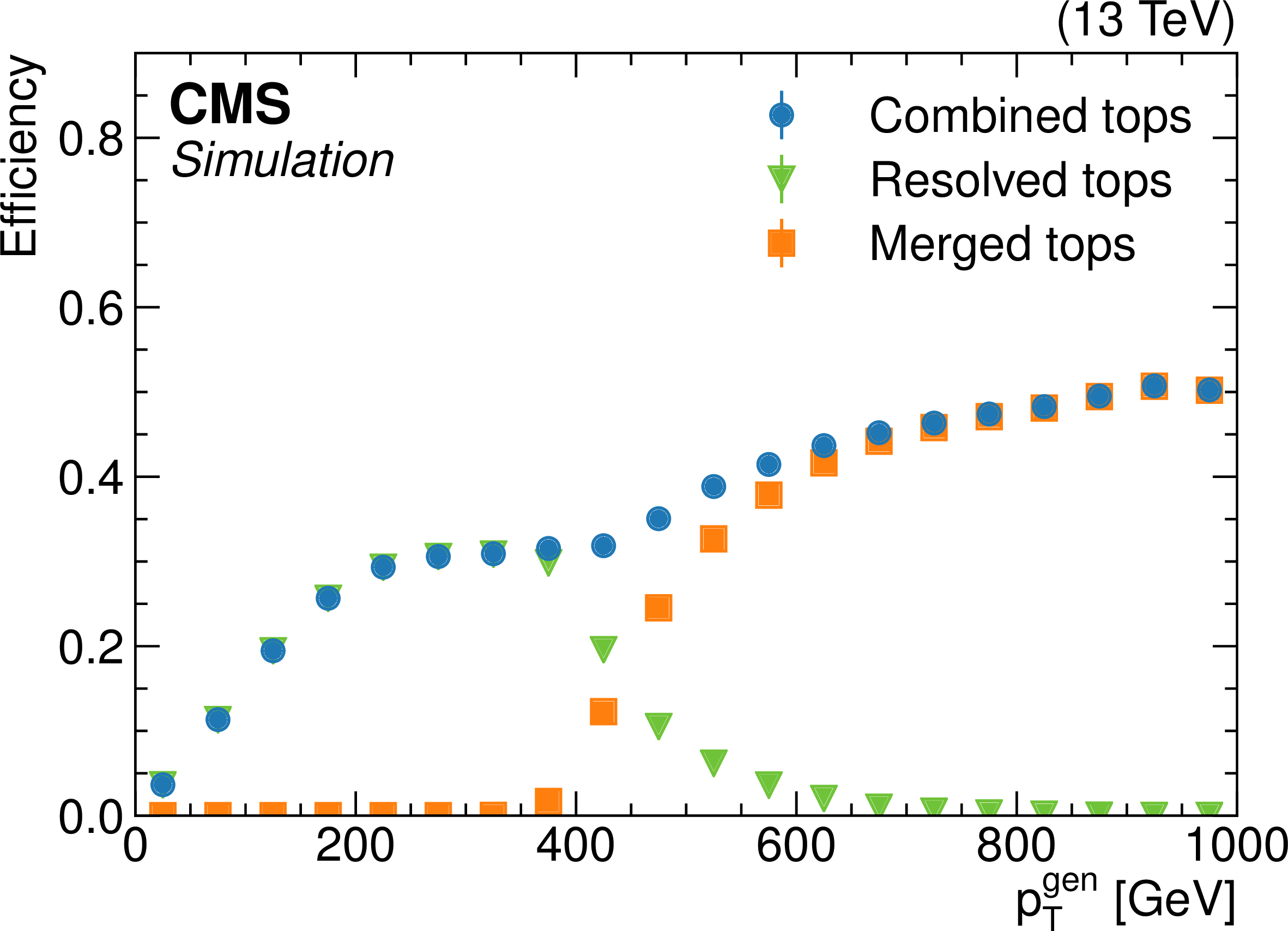
Figure 3-a:
Top quark tagging efficiencies are shown as a function of the generator-level top quark ${p_{\mathrm {T}}}$ for the merged tagging algorithm and resolved tagging algorithm described in Section 5.2. The plot shows the efficiencies as calculated in a sample of simulated ${\mathrm{t} {}\mathrm{\bar{t}}}$ events in which one top quark decays leptonically, while the other decays hadronically. In addition to the individual algorithms shown as orange squares (boosted top quarks) and green inverted triangles (resolved top quarks), the total top quark tagging efficiency (blue dots) is also shown. |

png pdf |
Figure 3-b:
Boosted W boson tagging efficiency shown as a function of the generator-level W boson ${p_{\mathrm {T}}}$ for the merged tagging algorithm described in Section 5.2. The plot shows the tagging efficiency (red triangles) when calculated in a sample of simulated WW events. |
png pdf |
Figure 4:
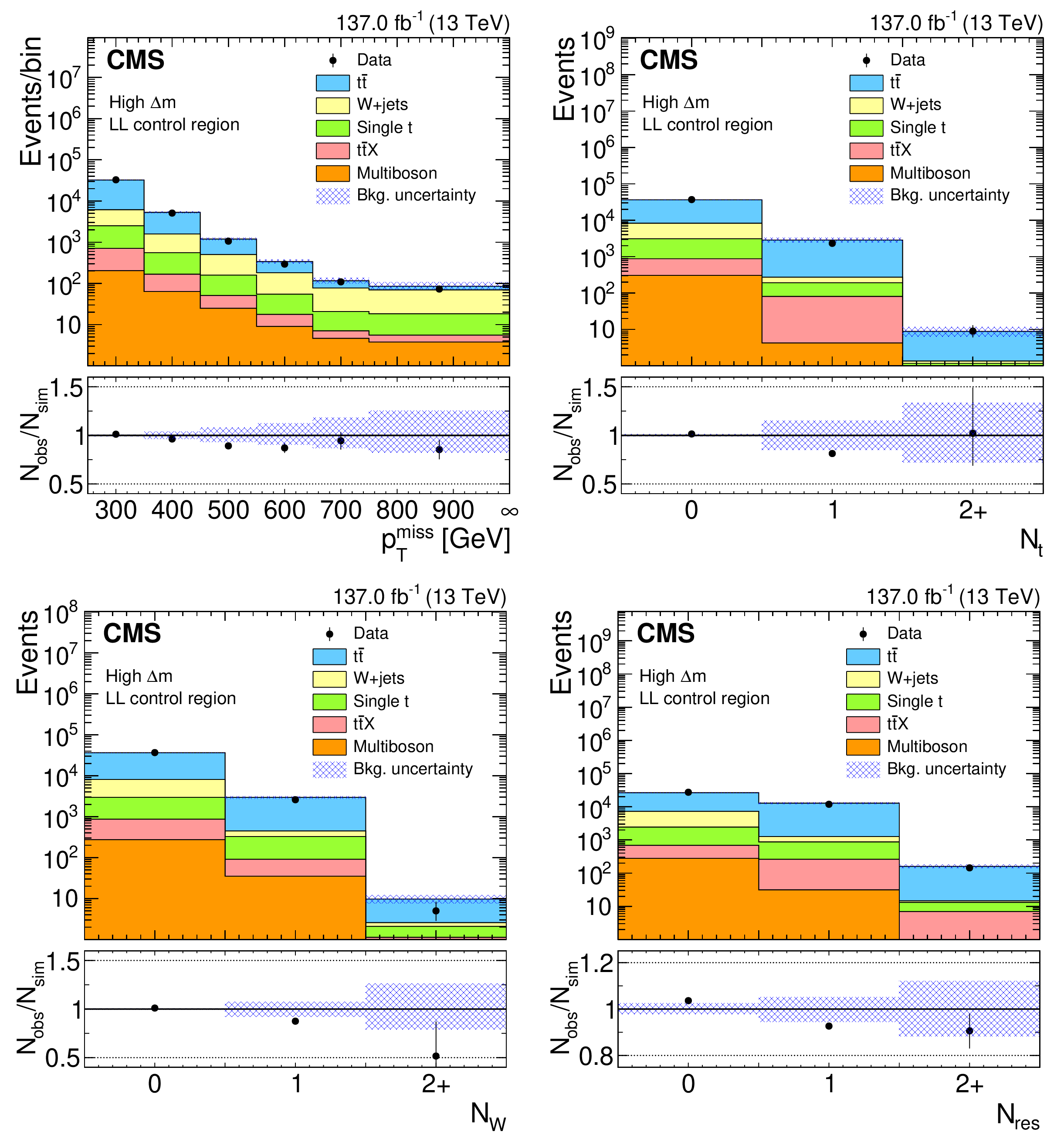
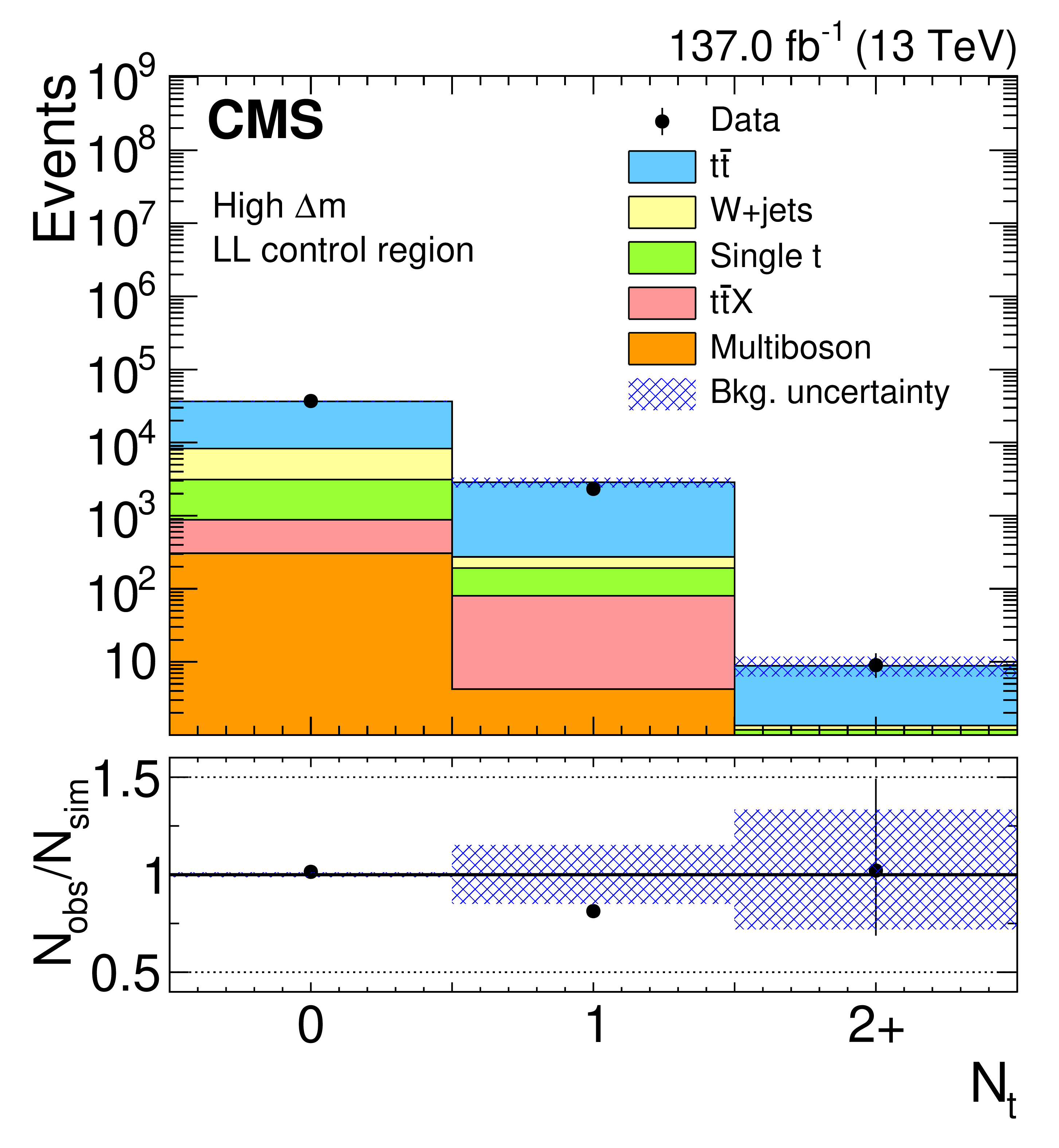
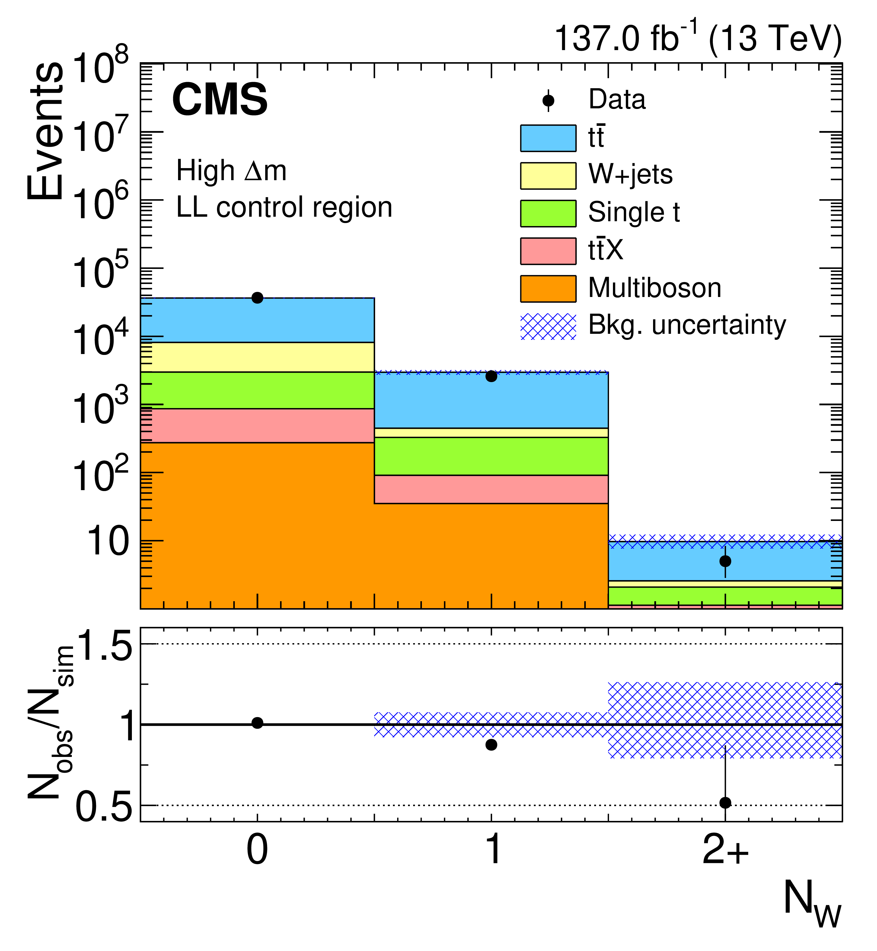
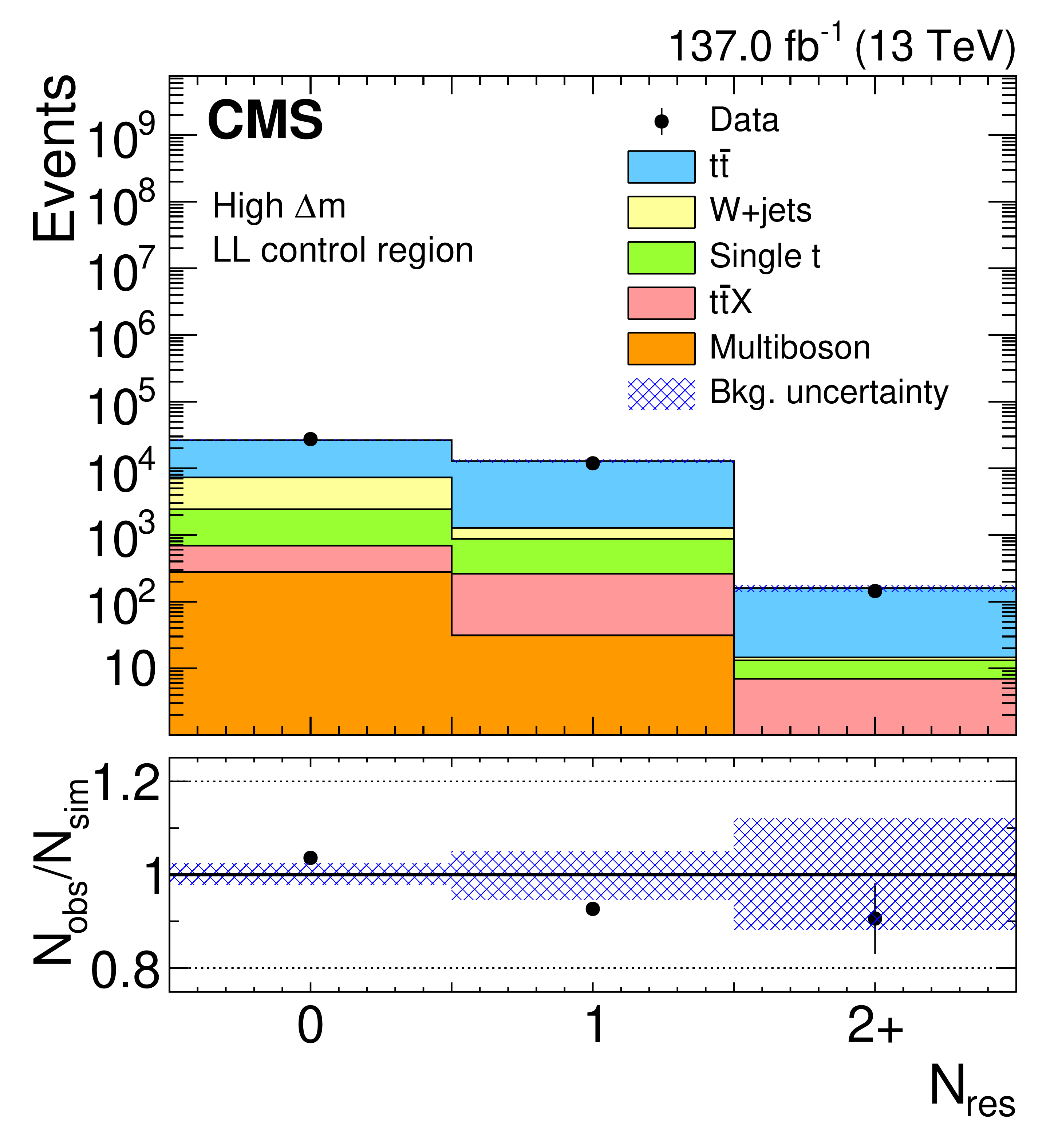
Comparison between data and simulation in the high ${\Delta m}$ portion of the $\ell$+jets control region, as a function of ${{p_{\mathrm {T}}} ^\text {miss}}$ (upper left), $N_{\mathrm{t}}$ (upper right), $N_{\mathrm{W}}$ (lower left), and $N_{\text{res}}$ (lower right) after scaling the simulation to match the total yield in data. The hatched region indicates the total shape uncertainty in the simulation. The lower panels display the ratios between the observed data and the simulation. |

png pdf |
Figure 4-a:
Comparison between data and simulation in the high ${\Delta m}$ portion of the $\ell$+jets control region, as a function of ${{p_{\mathrm {T}}} ^\text {miss}}$ after scaling the simulation to match the total yield in data. The hatched region indicates the total shape uncertainty in the simulation. The lower panel displays the ratios between the observed data and the simulation. |
png pdf |
Figure 4-b:
Comparison between data and simulation in the high ${\Delta m}$ portion of the $\ell$+jets control region, as a function of $N_{\mathrm{t}}$ after scaling the simulation to match the total yield in data. The hatched region indicates the total shape uncertainty in the simulation. The lower panel displays the ratios between the observed data and the simulation. |
png pdf |
Figure 4-c:
Comparison between data and simulation in the high ${\Delta m}$ portion of the $\ell$+jets control region, as a function of $N_{\mathrm{W}}$ after scaling the simulation to match the total yield in data. The hatched region indicates the total shape uncertainty in the simulation. The lower panel displays the ratios between the observed data and the simulation. |
png pdf |
Figure 4-d:
Comparison between data and simulation in the high ${\Delta m}$ portion of the $\ell$+jets control region, as a function of $N_{\text{res}}$ after scaling the simulation to match the total yield in data. The hatched region indicates the total shape uncertainty in the simulation. The lower panel displays the ratios between the observed data and the simulation. |
png pdf |
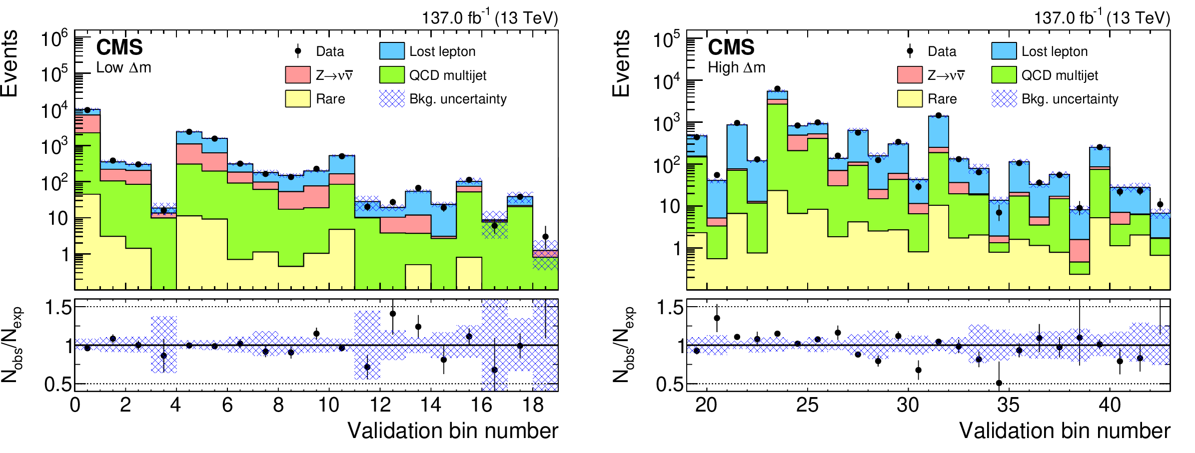
Figure 5:
The observed numbers of events and the SM background predictions for the low ${\Delta m}$ validation bins (left) and for the high ${\Delta m}$ validation bins (right). The hatched region indicates the total uncertainty in the background predictions. The lower panels display the ratios between the data and the SM predictions. |
png pdf |
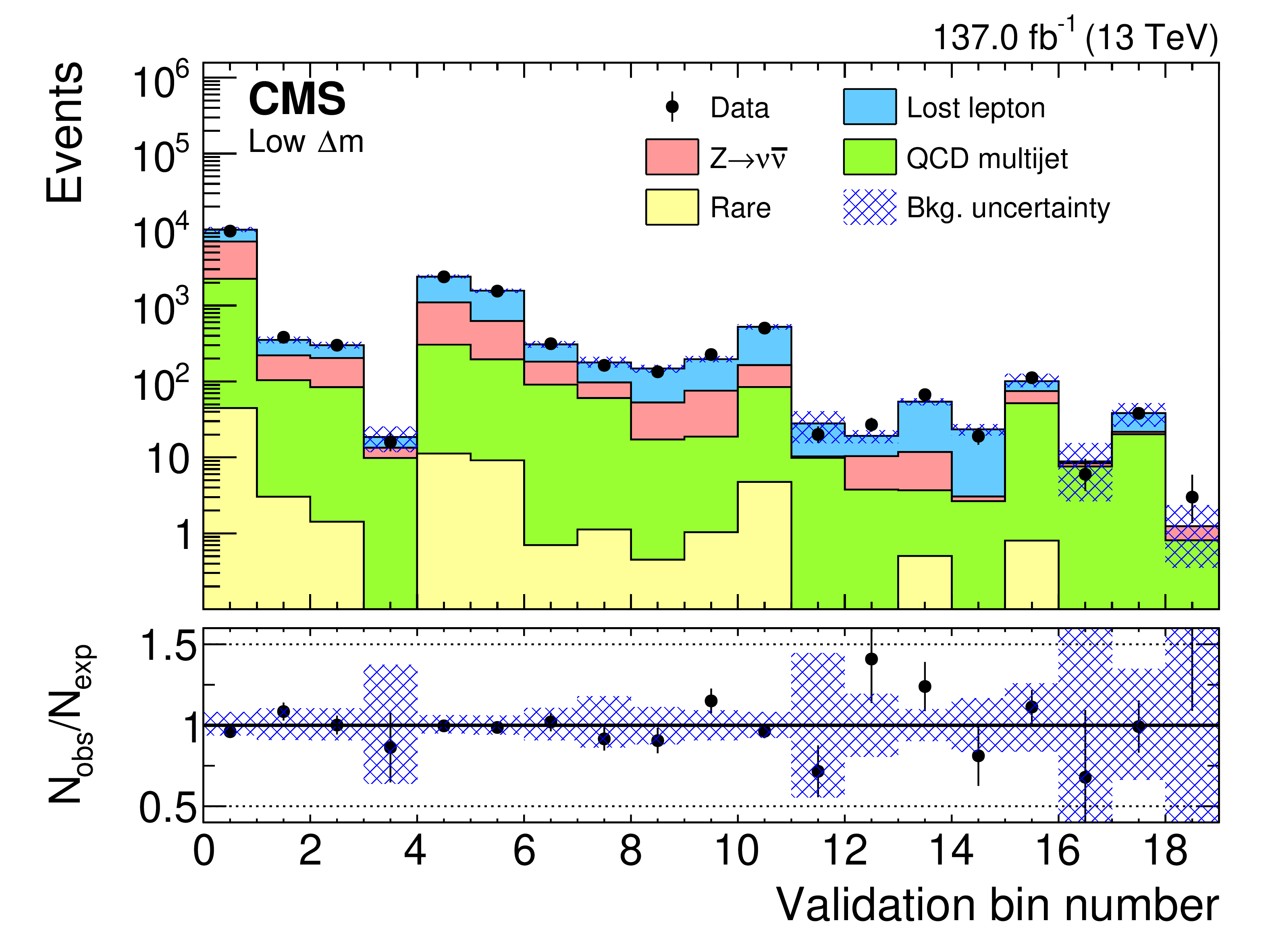
Figure 5-a:
The observed numbers of events and the SM background predictions for the low ${\Delta m}$ validation bins. The hatched region indicates the total uncertainty in the background predictions. The lower panel displays the ratios between the data and the SM predictions. |
png pdf |
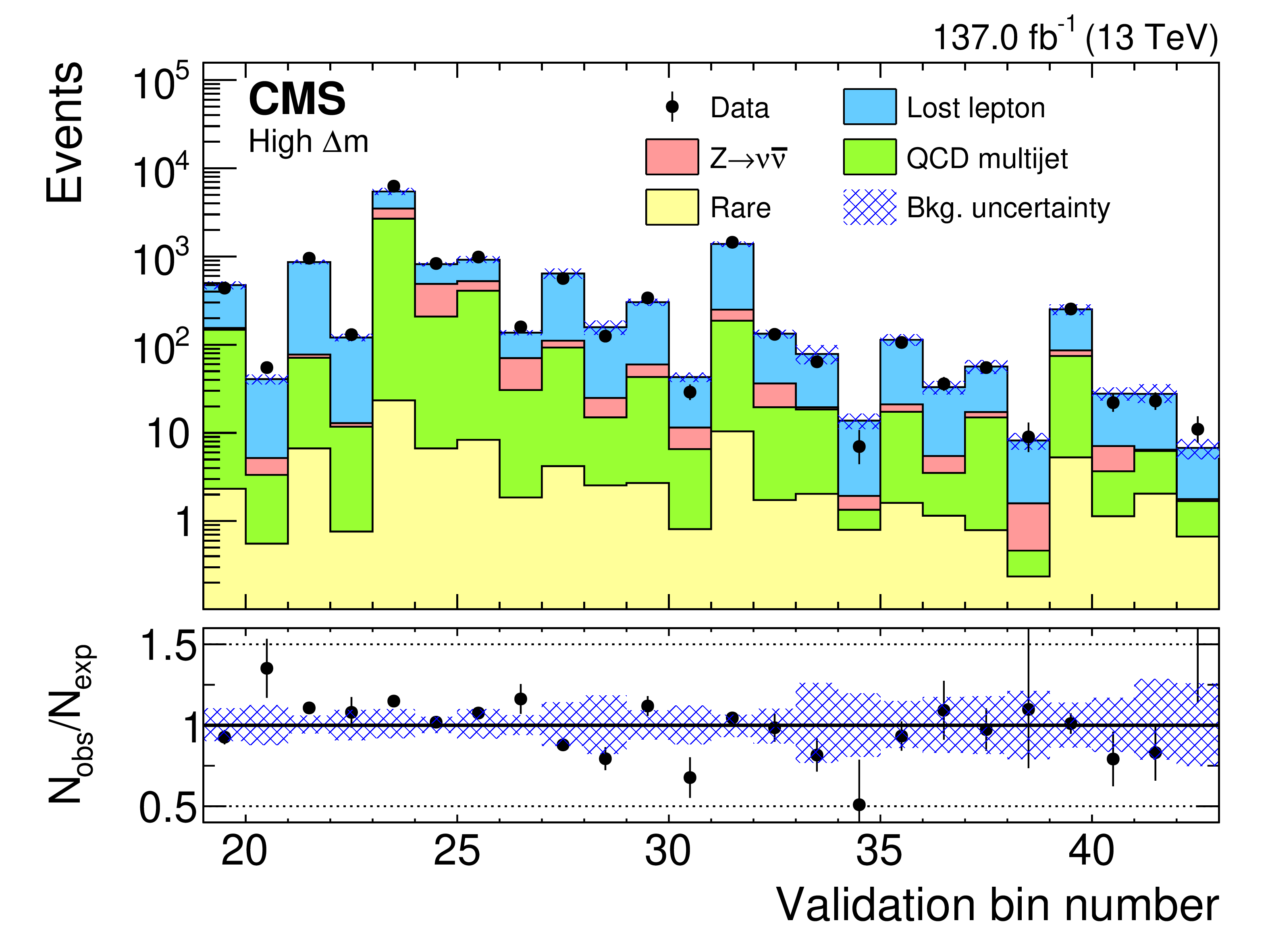
Figure 5-b:
The observed numbers of events and the SM background predictions for the high ${\Delta m}$ validation bins. The hatched region indicates the total uncertainty in the background predictions. The lower panel displays the ratios between the data and the SM predictions. |
png pdf |
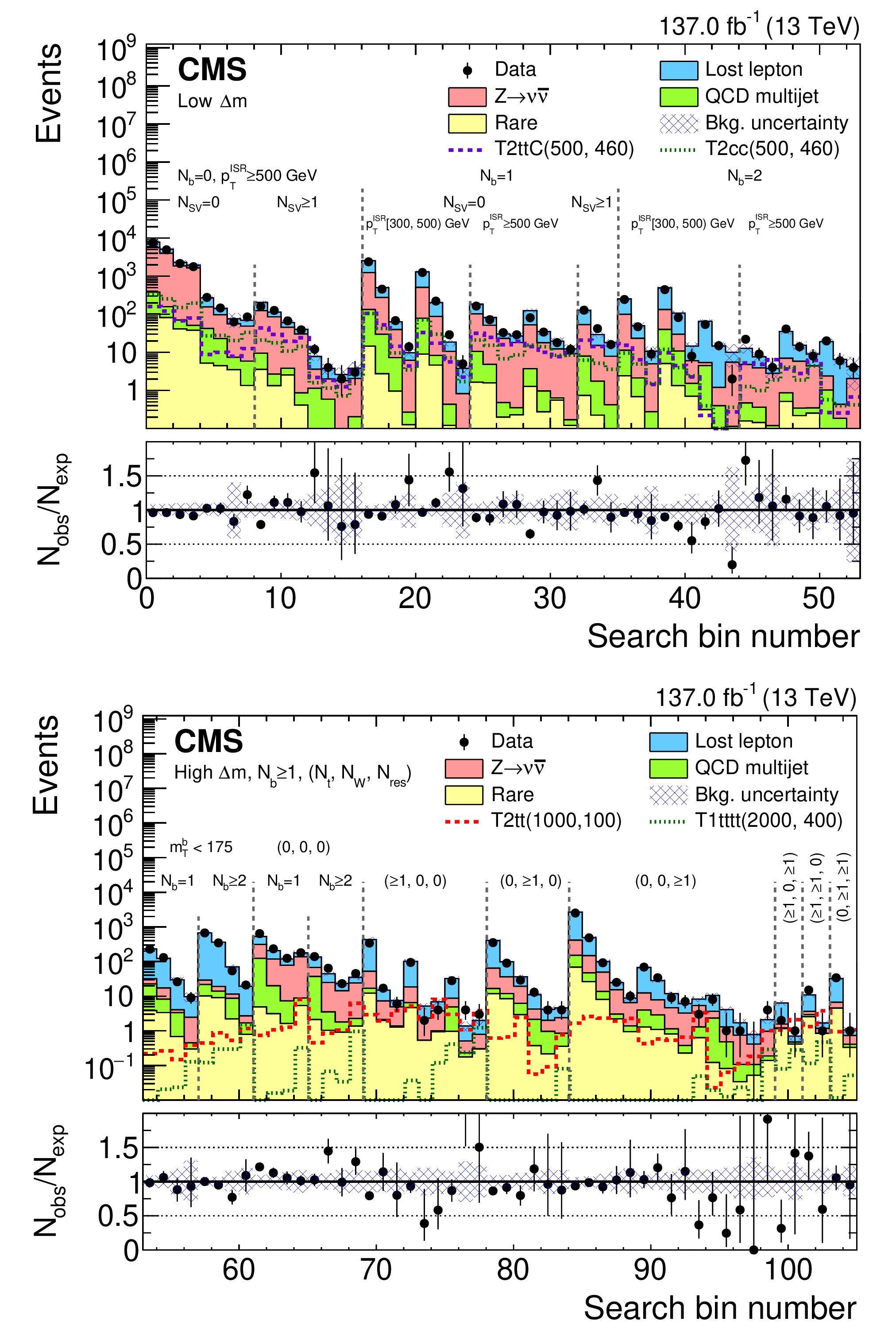
Figure 6:
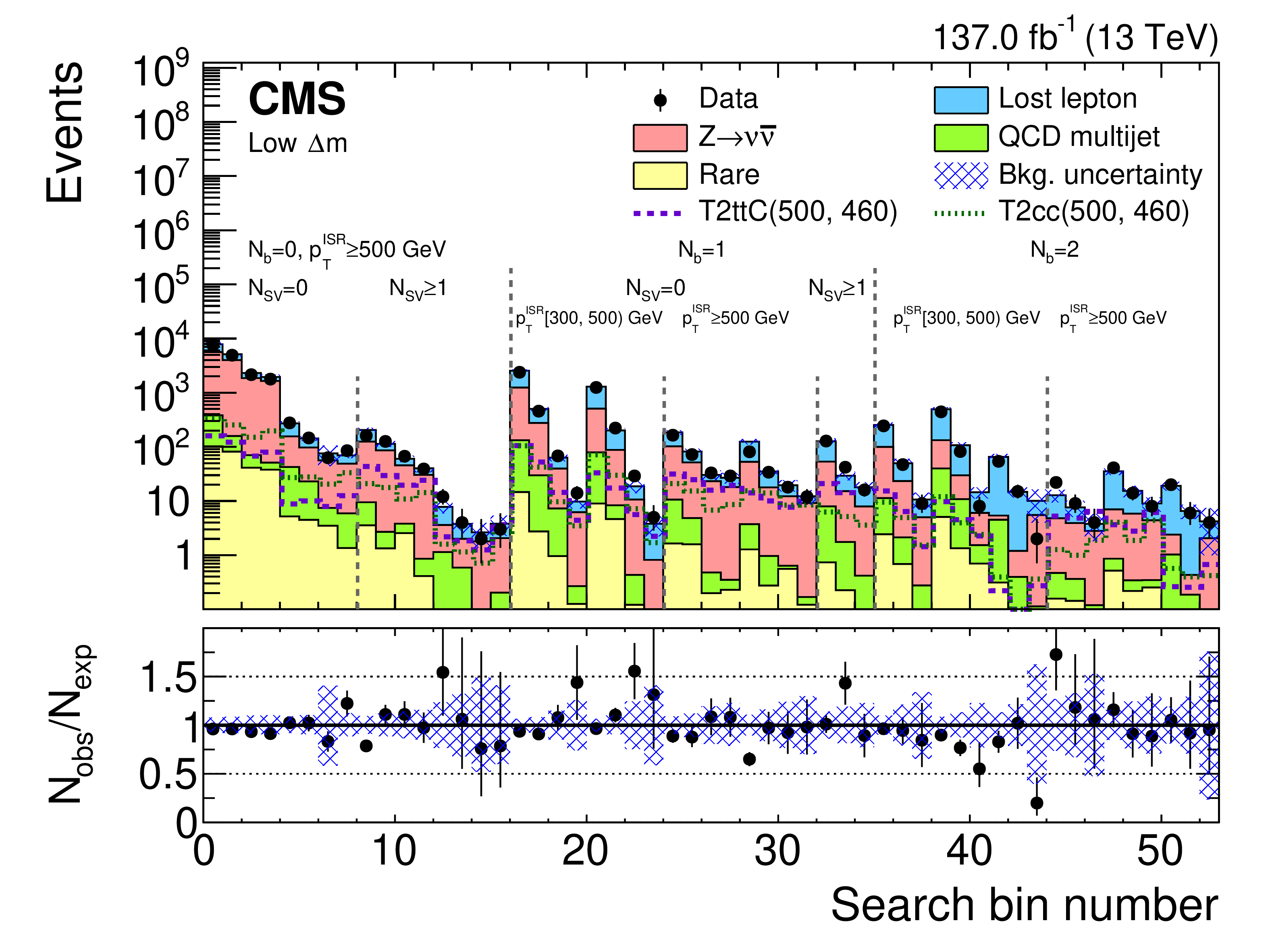
Observed event yields in data (black points) and predicted SM background (filled histograms) for the low ${\Delta m}$ search bins 0-52 (upper), and for the high ${\Delta m}$ search bins 53-104 (lower). The bracketed numbers in the lower plot represent the respective ${N_{\mathrm{t}}}$, ${N_{\mathrm{W}}}$, and ${N_{\text {res}}}$ requirements used in that region. The signal models are denoted in the legend with the masses in GeV of the SUSY particles in parentheses: $({m_{\tilde{\mathrm{t}}}}, {m_{\tilde{\chi}^0_1}})$ or $({m_{{\mathrm{\widetilde{g}}}}}, {m_{\tilde{\chi}^0_1}})$ for the T2 or T1 signal models, respectively. For both plots, the lower panel shows the ratio of the data to the total background prediction. The hatched bands correspond to the total uncertainty in the background prediction. The (unstacked) distributions for two example signal models are also shown in both plots. |
png pdf |
Figure 6-a:
Observed event yields in data (black points) and predicted SM background (filled histograms) for the low ${\Delta m}$ search bins 0-52. The signal T2 models are denoted in the legend with the masses in GeV of the SUSY particles in parentheses, $({m_{\tilde{\mathrm{t}}}}, {m_{\tilde{\chi}^0_1}})$. The lower panel shows the ratio of the data to the total background prediction. The hatched band corresponds to the total uncertainty in the background prediction. The (unstacked) distributions for two example signal models are also shown. |

png pdf |
Figure 6-b:
Observed event yields in data (black points) and predicted SM background (filled histograms) for the high ${\Delta m}$ search bins 53-104. The bracketed numbers represent the respective ${N_{\mathrm{t}}}$, ${N_{\mathrm{W}}}$, and ${N_{\text {res}}}$ requirements used in that region. The signal models are denoted in the legend with the masses in GeV of the SUSY particles in parentheses, $({m_{\tilde{\mathrm{t}}}}, {m_{\tilde{\chi}^0_1}})$ or $({m_{{\mathrm{\widetilde{g}}}}}, {m_{\tilde{\chi}^0_1}})$, for the T2 or T1 signal models. The lower panel shows the ratio of the data to the total background prediction. The hatched band corresponds to the total uncertainty in the background prediction. The (unstacked) distributions for two example signal models are also shown. |

png pdf |
Figure 7:
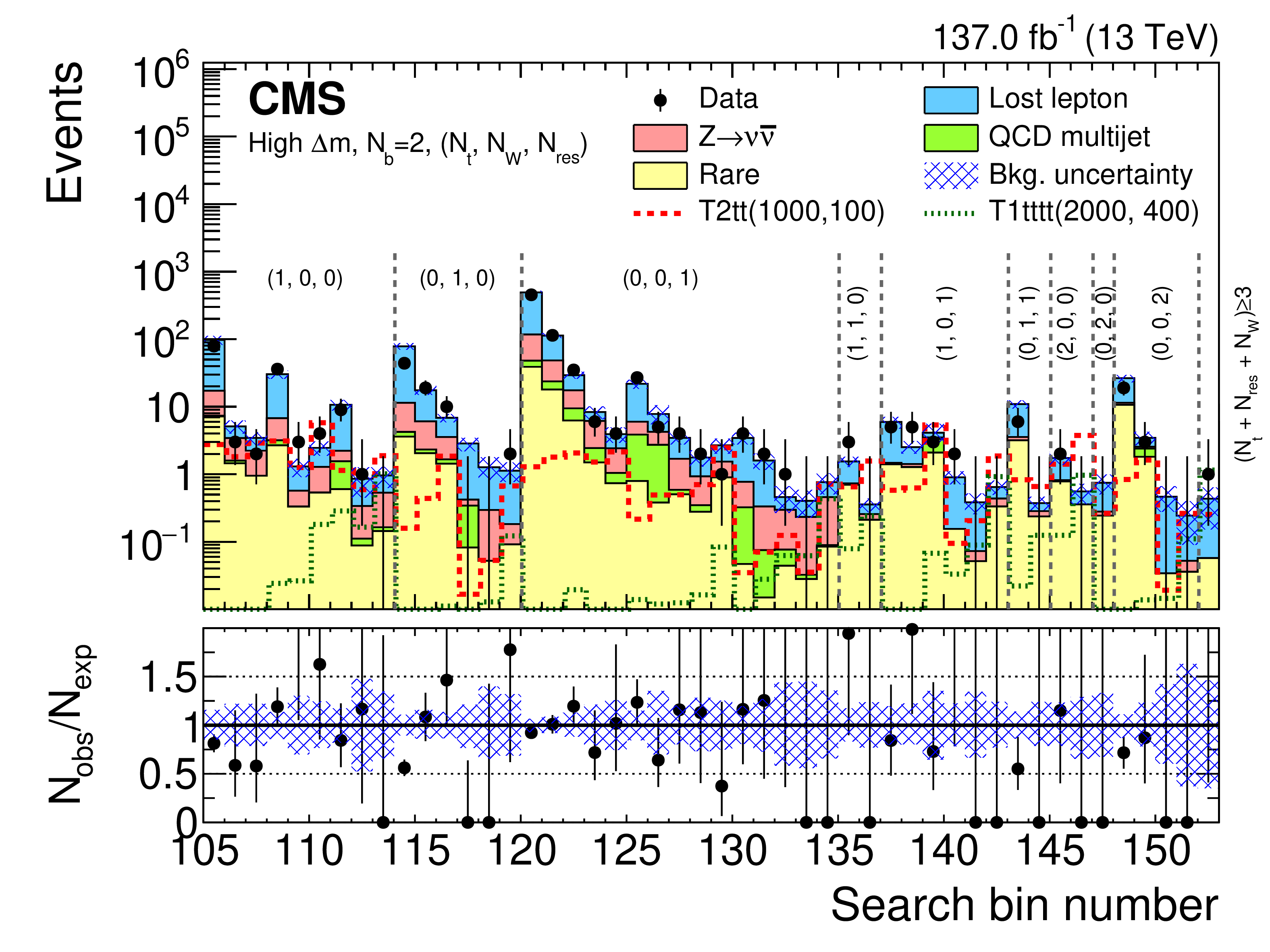
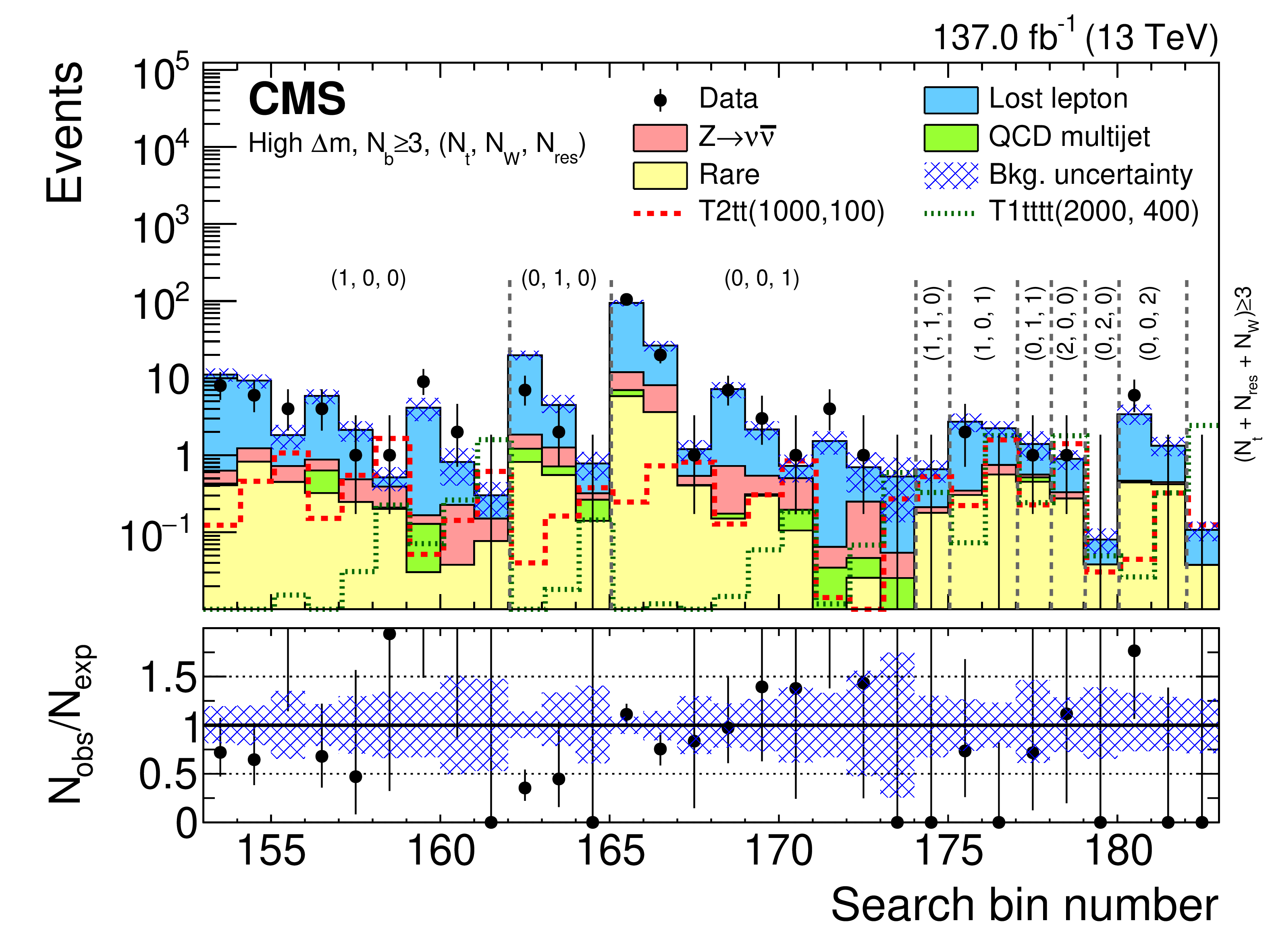
Observed event yields in data (black points) and predicted SM background (filled histograms) for the high ${\Delta m}$ search bins 105-152 with ${{N_{\mathrm{b}}} = 2}$ (upper), and for the high ${\Delta m}$ search bins 153-182 with ${{N_{\mathrm{b}}} \geq 3}$ (lower). The bracketed numbers in each plot represent the respective ${N_{\mathrm{t}}}$, ${N_{\mathrm{W}}}$, and ${N_{\text {res}}}$ requirements used in that region. The signal models are denoted in the legend with the masses in GeV of the SUSY particles in parentheses: $({m_{\tilde{\mathrm{t}}}}, {m_{\tilde{\chi}^0_1}})$ or $({m_{{\mathrm{\widetilde{g}}}}}, {m_{\tilde{\chi}^0_1}})$ for the T2 or T1 signal models, respectively. For both plots, the lower panel shows the ratio of the data to the total background prediction. The hatched bands correspond to the total uncertainty in the background prediction. The (unstacked) distributions for two example signal models are also shown in both plots. |
png pdf |
Figure 7-a:
Observed event yields in data (black points) and predicted SM background (filled histograms) for the high ${\Delta m}$ search bins 105-152 with ${{N_{\mathrm{b}}} = 2}$. The bracketed numbers represent the respective ${N_{\mathrm{t}}}$, ${N_{\mathrm{W}}}$, and ${N_{\text {res}}}$ requirements used in that region. The signal models are denoted in the legend with the masses in GeV of the SUSY particles in parentheses: $({m_{\tilde{\mathrm{t}}}}, {m_{\tilde{\chi}^0_1}})$ or $({m_{{\mathrm{\widetilde{g}}}}}, {m_{\tilde{\chi}^0_1}})$ for the T2 or T1 signal models, respectively. The lower panel shows the ratio of the data to the total background prediction. The hatched band corresponds to the total uncertainty in the background prediction. The (unstacked) distributions for two example signal models are also shown. |
png pdf |
Figure 7-b:
Observed event yields in data (black points) and predicted SM background (filled histograms) for the high ${\Delta m}$ search bins 153-182 with ${{N_{\mathrm{b}}} \geq 3}$. The bracketed numbers represent the respective ${N_{\mathrm{t}}}$, ${N_{\mathrm{W}}}$, and ${N_{\text {res}}}$ requirements used in that region. The signal models are denoted in the legend with the masses in GeV of the SUSY particles in parentheses: $({m_{\tilde{\mathrm{t}}}}, {m_{\tilde{\chi}^0_1}})$ or $({m_{{\mathrm{\widetilde{g}}}}}, {m_{\tilde{\chi}^0_1}})$ for the T2 or T1 signal models, respectively. The lower panel shows the ratio of the data to the total background prediction. The hatched band corresponds to the total uncertainty in the background prediction. The (unstacked) distributions for two example signal models are also shown. |
png pdf |
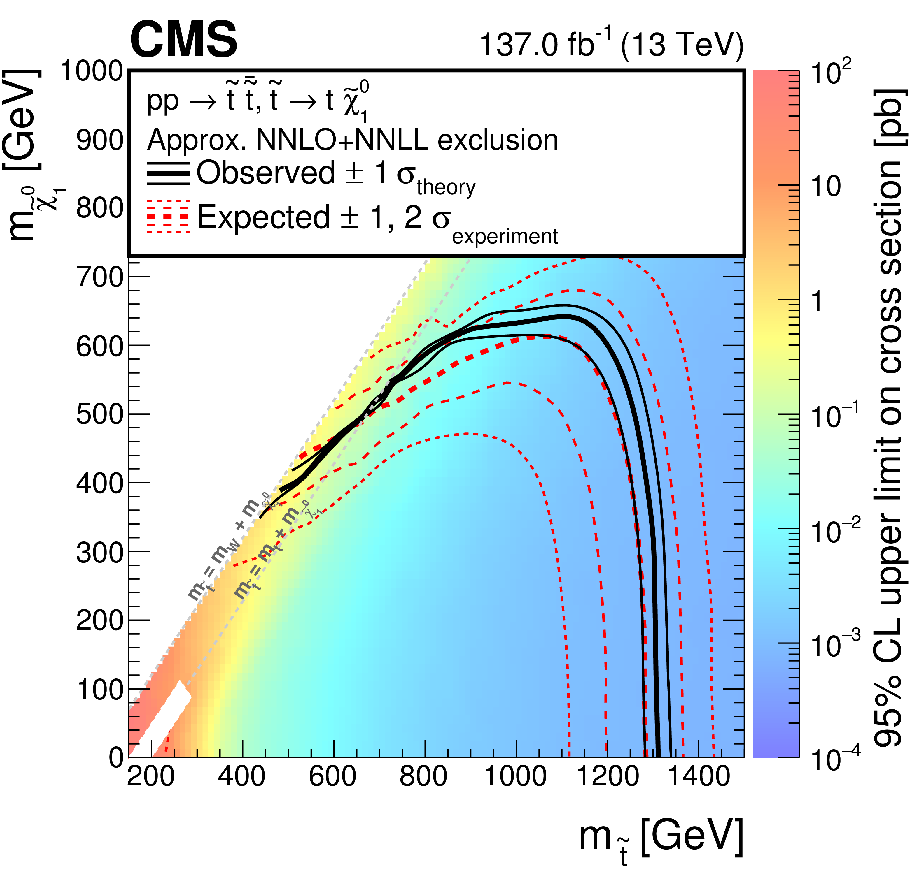
Figure 8:
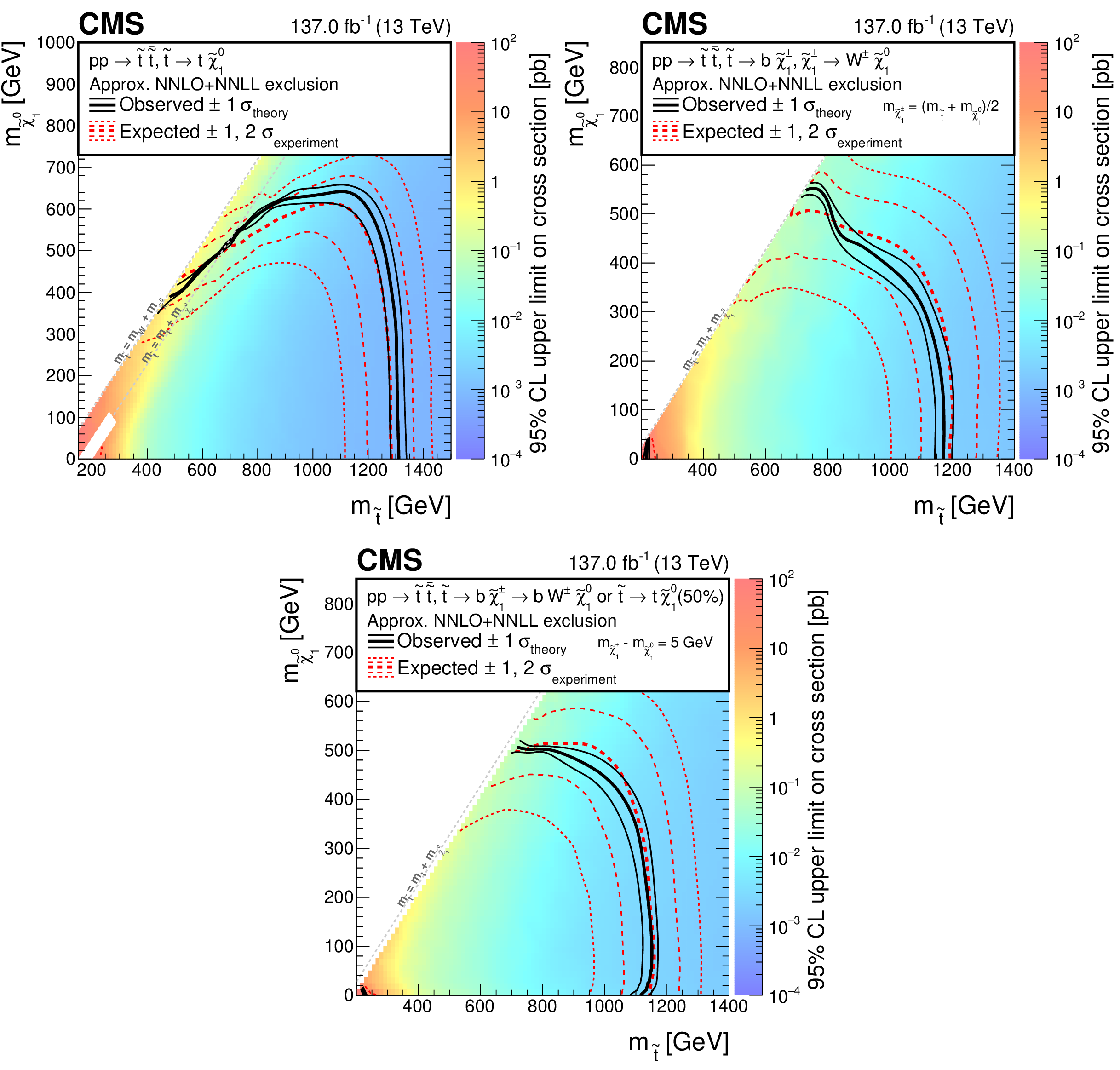
The 95% CL upper limit on the production cross section of the T2tt (upper left), T2bW (upper right), and T2tb (lower) simplified models as a function of the top squark and LSP masses. The solid black curves represent the observed exclusion contour with respect to approximate NNLO+NNLL signal cross sections and the change in this contour due to variation of these cross sections within their theoretical uncertainties ($\sigma _{\text {theory}}$) [64,65,66,67,68,69,70,71,72,73,74]. The dashed red curves indicate the mean expected exclusion contour and the region containing 68 and 95% ($\pm$1 and 2$\sigma _{\text {experiment}}$) of the distribution of expected exclusion limits under the background-only hypothesis. For T2tt, no interpretation is provided for signal models for which ${| {m_{\tilde{\mathrm{t}}}} - {m_{\tilde{\chi}^0_1}} - {m_{\mathrm{t}}} |} < $ 25 GeV and ${m_{\tilde{\mathrm{t}}}} < $ 275 GeV as described in the text. |
png pdf |
Figure 8-a:
The 95% CL upper limit on the production cross section of the T2tt simplified model as a function of the top squark and LSP masses. The solid black curves represent the observed exclusion contour with respect to approximate NNLO+NNLL signal cross sections and the change in this contour due to variation of these cross sections within their theoretical uncertainties ($\sigma _{\text {theory}}$). The dashed red curves indicate the mean expected exclusion contour and the region containing 68 and 95% ($\pm$1 and 2$\sigma _{\text {experiment}}$) of the distribution of expected exclusion limits under the background-only hypothesis. For this model, no interpretation is provided for signal models for which ${| {m_{\tilde{\mathrm{t}}}} - {m_{\tilde{\chi}^0_1}} - {m_{\mathrm{t}}} |} < $ 25 GeV and ${m_{\tilde{\mathrm{t}}}} < $ 275 GeV as described in the text. |
png pdf |
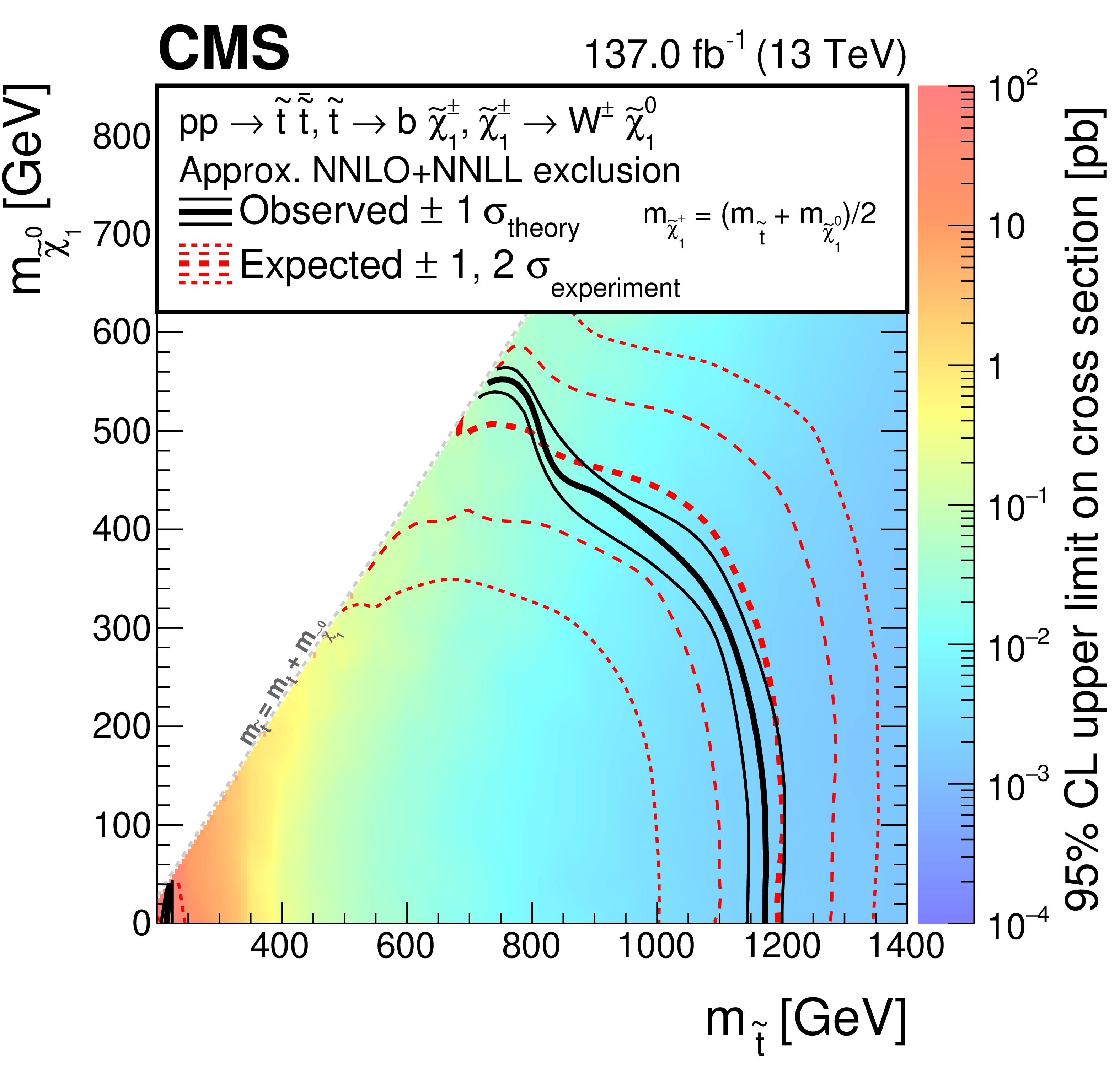
Figure 8-b:
The 95% CL upper limit on the production cross section of the T2bW simplified model as a function of the top squark and LSP masses. The solid black curves represent the observed exclusion contour with respect to approximate NNLO+NNLL signal cross sections and the change in this contour due to variation of these cross sections within their theoretical uncertainties ($\sigma _{\text {theory}}$). The dashed red curves indicate the mean expected exclusion contour and the region containing 68 and 95% ($\pm$1 and 2$\sigma _{\text {experiment}}$) of the distribution of expected exclusion limits under the background-only hypothesis. |
png pdf |
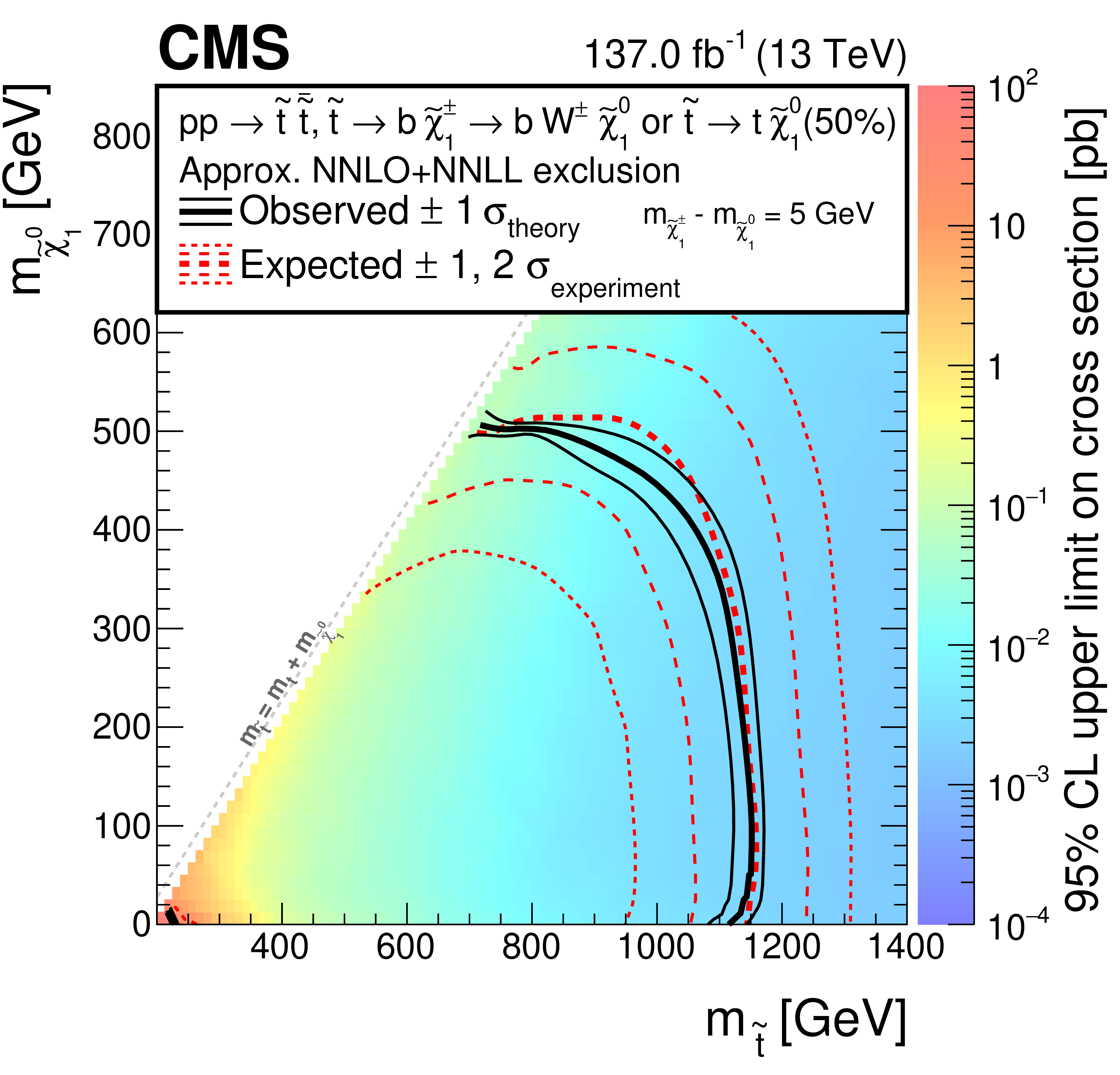
Figure 8-c:
The 95% CL upper limit on the production cross section of the T2tb simplified model as a function of the top squark and LSP masses. The solid black curves represent the observed exclusion contour with respect to approximate NNLO+NNLL signal cross sections and the change in this contour due to variation of these cross sections within their theoretical uncertainties ($\sigma _{\text {theory}}$). The dashed red curves indicate the mean expected exclusion contour and the region containing 68 and 95% ($\pm$1 and 2$\sigma _{\text {experiment}}$) of the distribution of expected exclusion limits under the background-only hypothesis. |
png pdf |
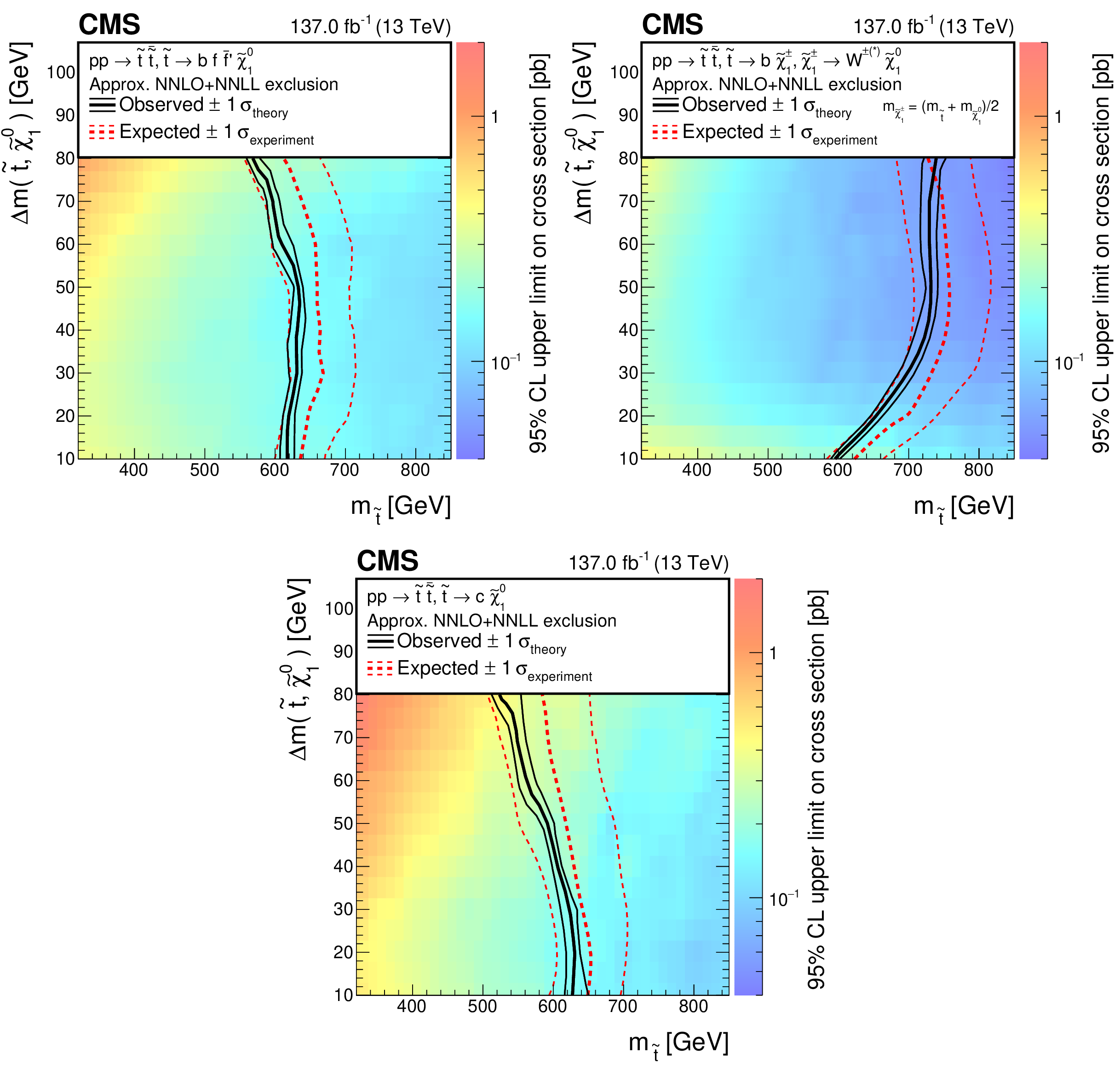
Figure 9:
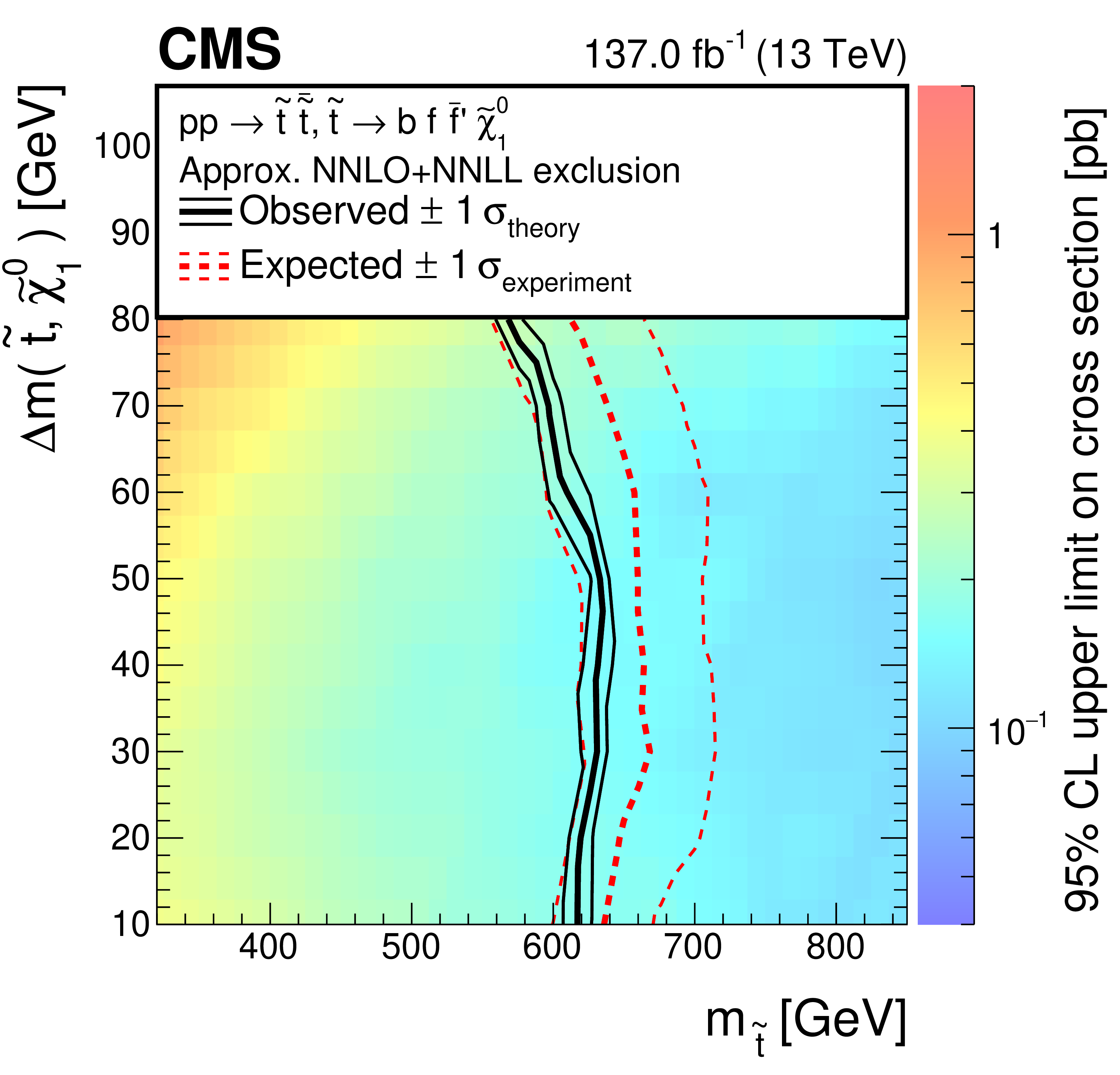
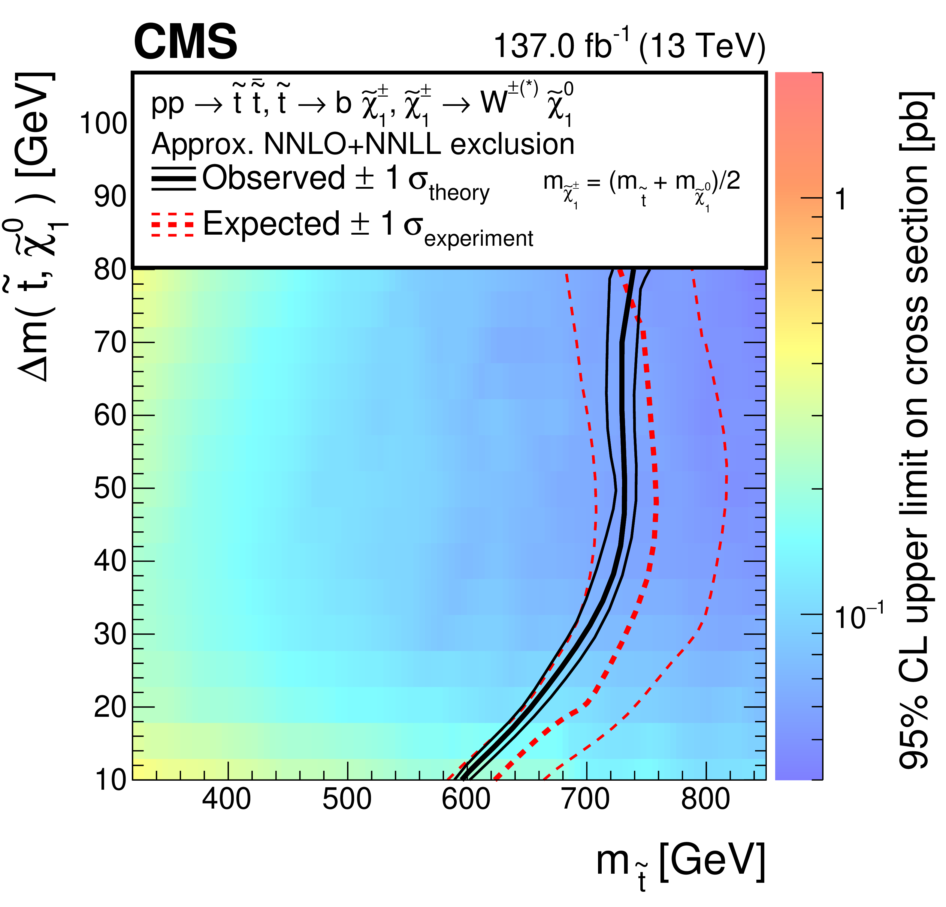
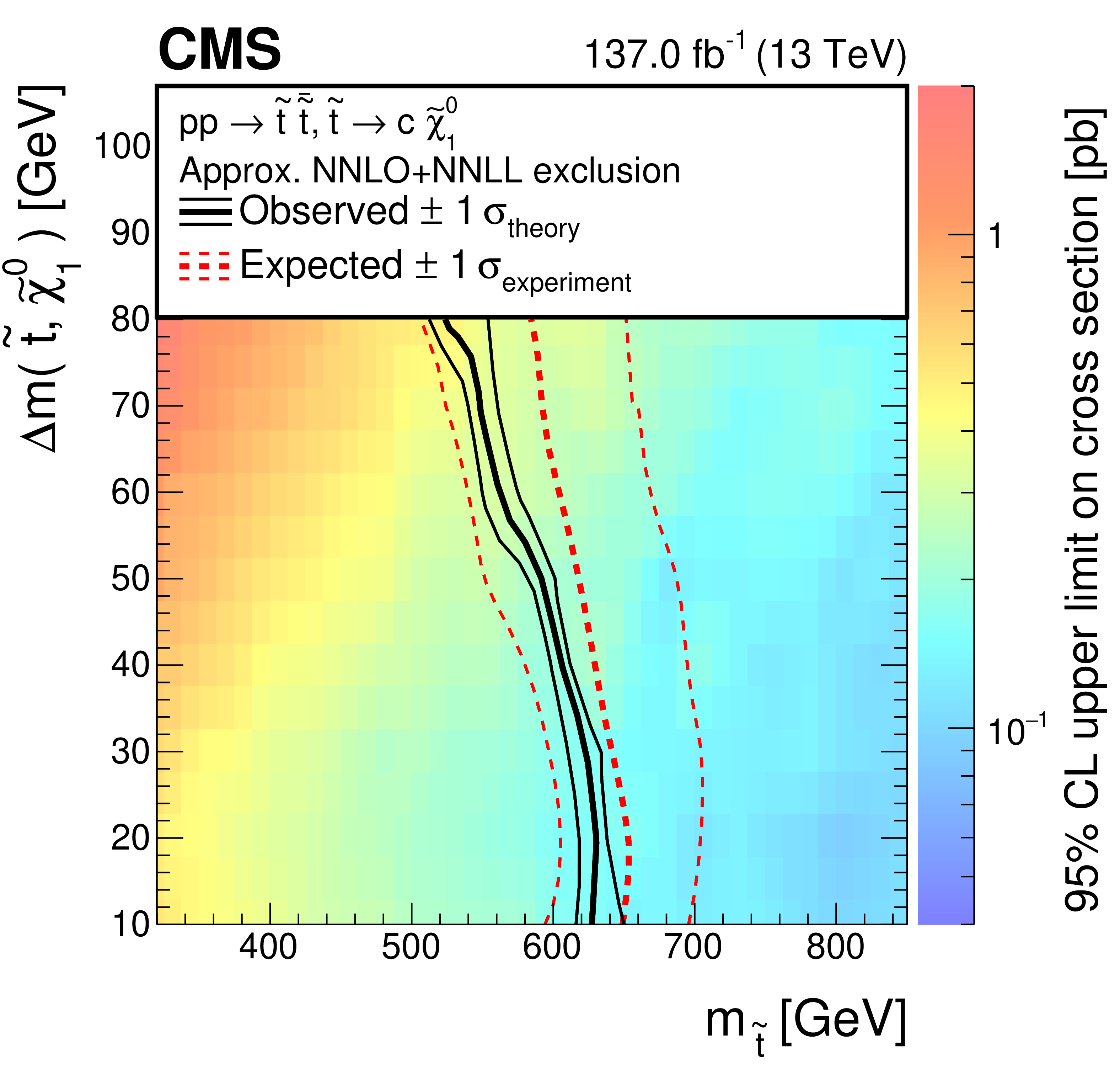
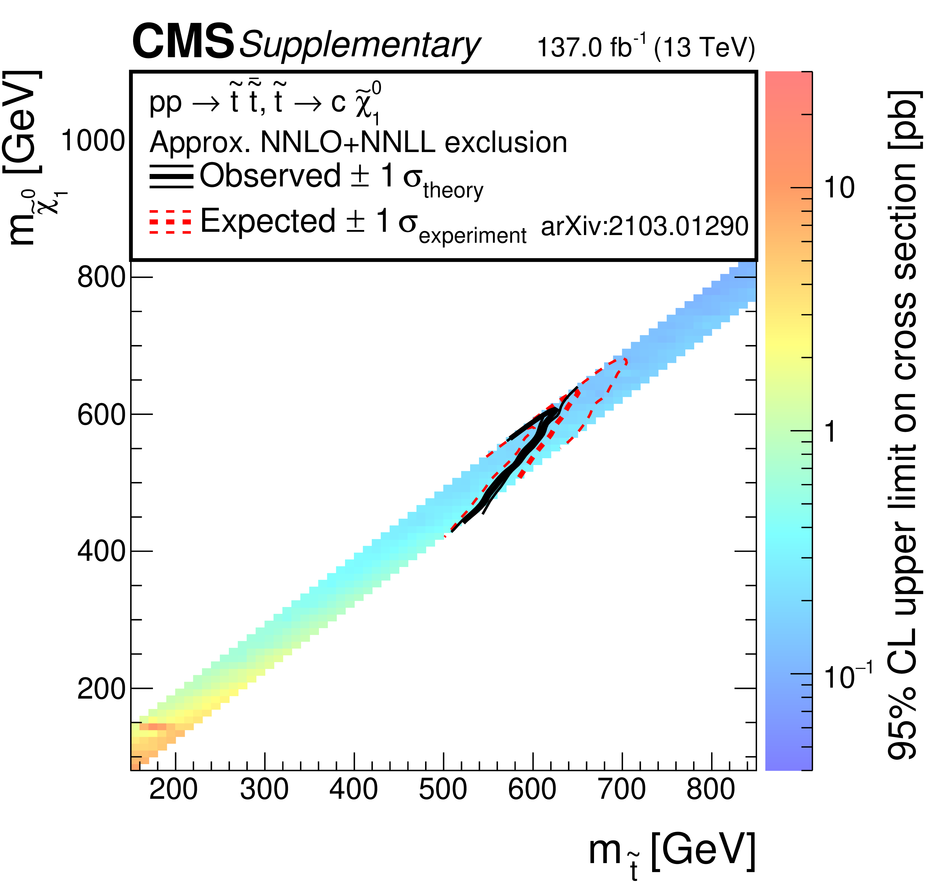
The 95% CL upper limit on the production cross section of the T2ttC (upper left), T2bWC (upper right), and T2cc (lower) simplified models as a function of the top squark mass and the difference between the top squark and LSP masses. The solid black curves represent the observed exclusion contour with respect to approximate NNLO+NNLL signal cross sections and the change in this contour due to variation of these cross sections within their theoretical uncertainties ($\sigma _{\text {theory}}$) [64,65,66,67,68,69,70,71,72,73,74]. The dashed red curves indicate the mean expected exclusion contour and the region containing 68% ($\pm$1$\sigma _{\text {experiment}}$) of the distribution of expected exclusion limits under the background-only hypothesis. |
png pdf |
Figure 9-a:
The 95% CL upper limit on the production cross section of the T2ttC simplified model as a function of the top squark mass and the difference between the top squark and LSP masses. The solid black curves represent the observed exclusion contour with respect to approximate NNLO+NNLL signal cross sections and the change in this contour due to variation of these cross sections within their theoretical uncertainties ($\sigma _{\text {theory}}$). The dashed red curves indicate the mean expected exclusion contour and the region containing 68% ($\pm$1$\sigma _{\text {experiment}}$) of the distribution of expected exclusion limits under the background-only hypothesis. |
png pdf |
Figure 9-b:
The 95% CL upper limit on the production cross section of the T2bWC simplified model as a function of the top squark mass and the difference between the top squark and LSP masses. The solid black curves represent the observed exclusion contour with respect to approximate NNLO+NNLL signal cross sections and the change in this contour due to variation of these cross sections within their theoretical uncertainties ($\sigma _{\text {theory}}$). The dashed red curves indicate the mean expected exclusion contour and the region containing 68% ($\pm$1$\sigma _{\text {experiment}}$) of the distribution of expected exclusion limits under the background-only hypothesis. |
png pdf |
Figure 9-c:
The 95% CL upper limit on the production cross section of the T2cc simplified model as a function of the top squark mass and the difference between the top squark and LSP masses. The solid black curves represent the observed exclusion contour with respect to approximate NNLO+NNLL signal cross sections and the change in this contour due to variation of these cross sections within their theoretical uncertainties ($\sigma _{\text {theory}}$). The dashed red curves indicate the mean expected exclusion contour and the region containing 68% ($\pm$1$\sigma _{\text {experiment}}$) of the distribution of expected exclusion limits under the background-only hypothesis. |
png pdf |
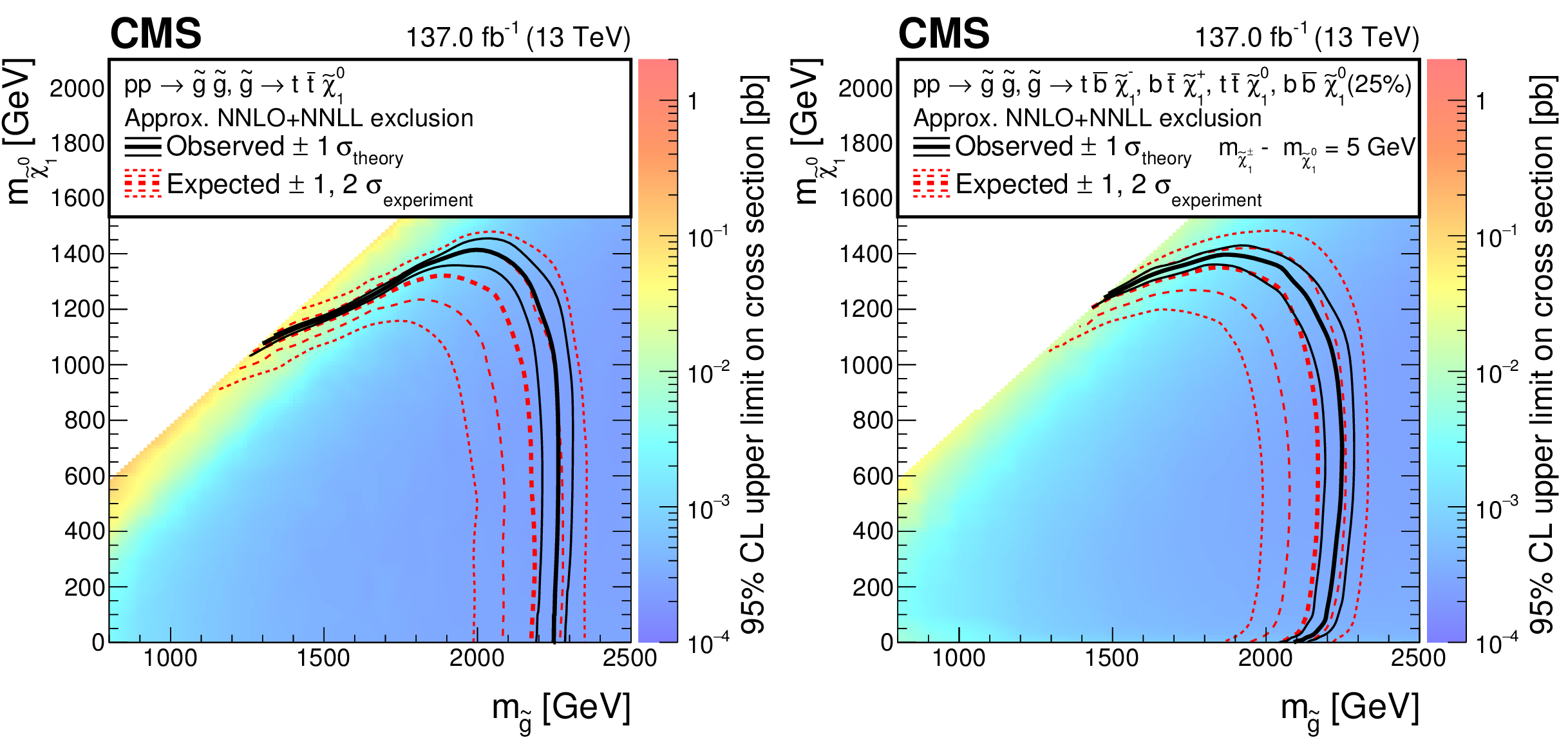
Figure 10:
The 95% CL upper limit on the production cross section of the T1tttt (left) and T1ttbb (right) simplified models as a function of the gluino and LSP masses. The solid black curves represent the observed exclusion contour with respect to approximate NNLO+NNLL signal cross sections and the change in this contour due to variation of these cross sections within their theoretical uncertainties ($\sigma _{\text {theory}}$) [64,65,66,67,68,69,70,71,72,73,74]. The dashed red curves indicate the mean expected exclusion contour and the region containing 68 and 95% ($\pm$1 and 2$\sigma _{\text {experiment}}$) of the distribution of expected exclusion limits under the background-only hypothesis. |

png pdf |
Figure 10-a:
The 95% CL upper limit on the production cross section of the T1tttt simplified model as a function of the gluino and LSP masses. The solid black curves represent the observed exclusion contour with respect to approximate NNLO+NNLL signal cross sections and the change in this contour due to variation of these cross sections within their theoretical uncertainties ($\sigma _{\text {theory}}$). The dashed red curves indicate the mean expected exclusion contour and the region containing 68 and 95% ($\pm$1 and 2$\sigma _{\text {experiment}}$) of the distribution of expected exclusion limits under the background-only hypothesis. |
png pdf |
Figure 10-b:
The 95% CL upper limit on the production cross section of the T1ttbb simplified model as a function of the gluino and LSP masses. The solid black curves represent the observed exclusion contour with respect to approximate NNLO+NNLL signal cross sections and the change in this contour due to variation of these cross sections within their theoretical uncertainties ($\sigma _{\text {theory}}$). The dashed red curves indicate the mean expected exclusion contour and the region containing 68 and 95% ($\pm$1 and 2$\sigma _{\text {experiment}}$) of the distribution of expected exclusion limits under the background-only hypothesis. |
png pdf |
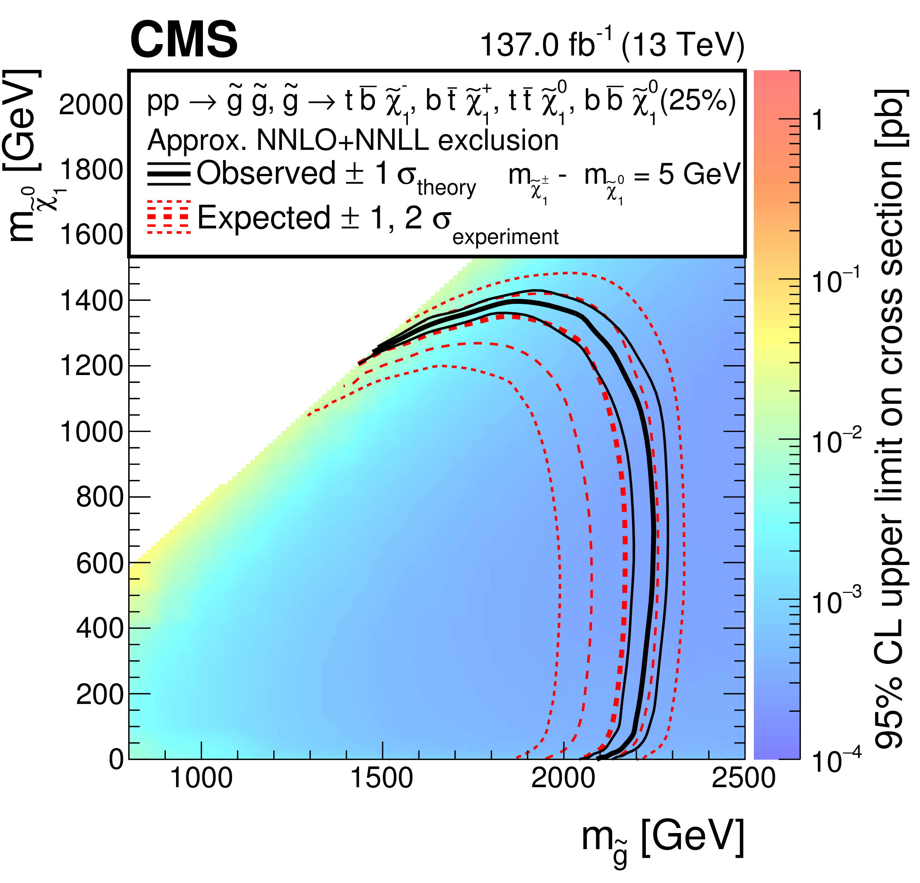
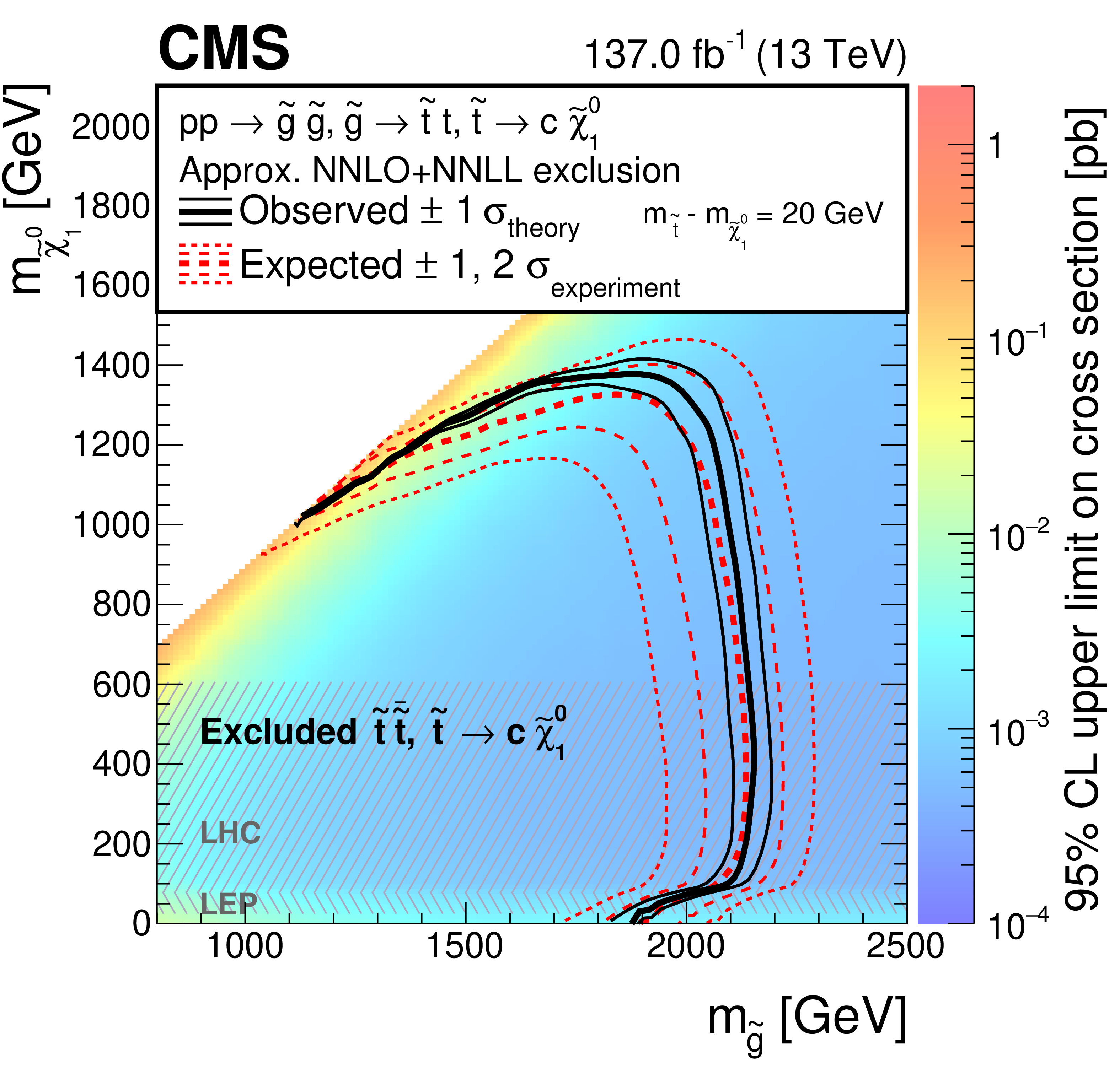
Figure 11:
The 95% CL upper limit on the production cross section of the T5ttcc simplified model as a function of the gluino and LSP masses. The solid black curves represent the observed exclusion contour with respect to approximate NNLO+NNLL signal cross sections and the change in this contour due to variation of these cross sections within their theoretical uncertainties ($\sigma _{\text {theory}}$) [64,65,66,67,68,69,70,71,72,73,74]. The dashed red curves indicate the mean expected exclusion contour and the region containing 68% and 95% ($\pm$1 and 2$\sigma _{\text {experiment}}$) of the distribution of expected exclusion limits under the background-only hypothesis. The expected and observed upper limits do not take into account contributions from direct top squark pair production; however, its effect is small for $ {m_{\tilde{\chi}^0_1}} > $ 600 GeV, which corresponds to the phase space beyond the exclusions based on direct top squark pair production. The excluded regions based on direct top squark pair production from this search and earlier searches by the ATLAS [27] and CMS [37,40,42] experiments, as well as by the LEP experiments [129,130,131,132] are indicated by the hatched areas. |
| Tables | |

png pdf |
Table 1:
Summary of the preselection requirements (baseline selection) imposed on the reconstructed physics objects for this search, as well as the low ${\Delta m}$ and high ${\Delta m}$ baseline selections. Here $R$ is the distance parameter of the anti-$ {k_{\mathrm {T}}}$ algorithm. Electron and muon candidates as well as ${\tau _\mathrm {h}}$ candidates and isolated tracks are as defined in Section 5. The $i$-th highest- ${p_{\mathrm {T}}}$ jet is denoted by ${\mathrm {j}_{i}}$. |
png pdf |
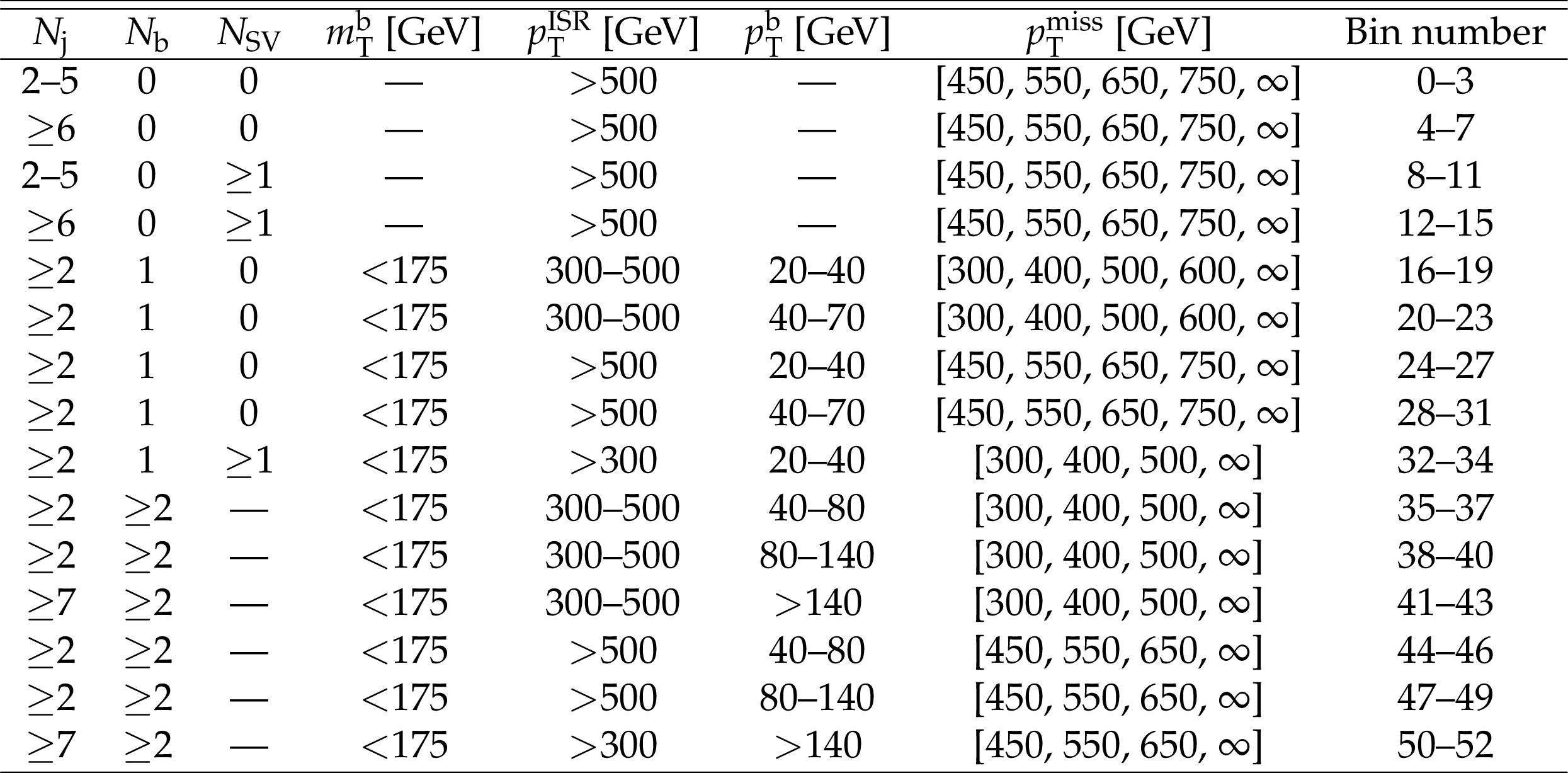
Table 2:
Summary of the 53 search bins that mainly target low ${\Delta m}$ signal models. For these search bins, events are required to pass the low ${\Delta m}$ region selection discussed in Section 6.1. Within each row of this table, the bins are ordered by increasing ${{p_{\mathrm {T}}} ^\text {miss}}$ requirements. A dash (--) indicates that no requirements are made. |
png pdf |
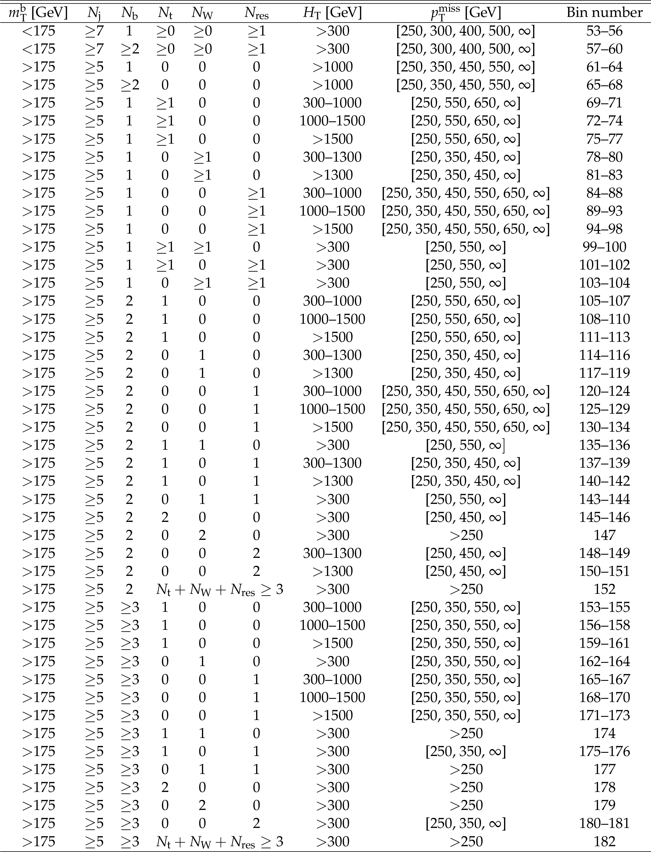
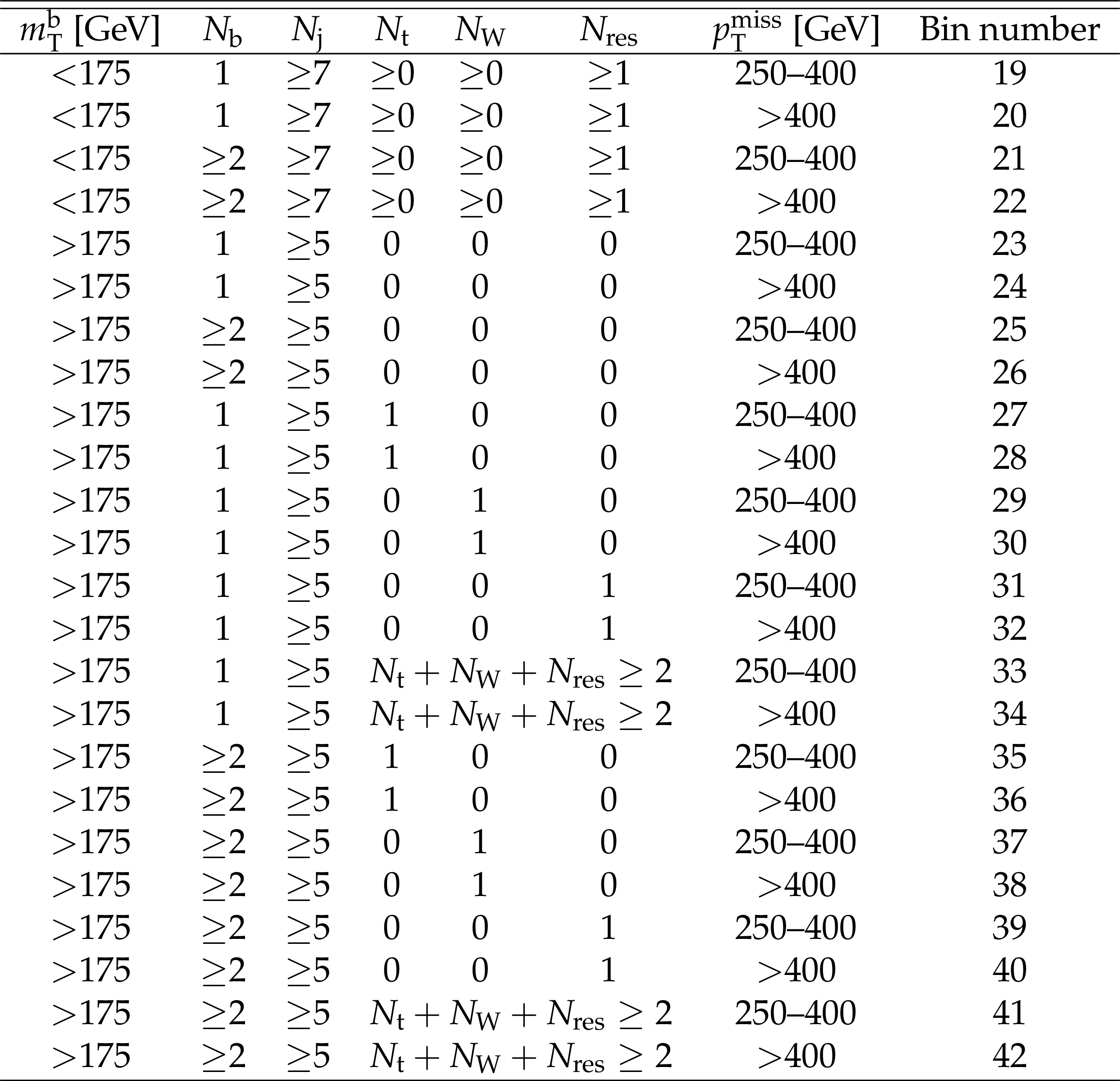
Table 3:
Summary of the 130 search bins that mainly target high ${\Delta m}$ signal models. For these search bins, events are required to pass the high ${\Delta m}$ region selection discussed in Section 6.2. Within each row of this table, the bins are ordered by increasing ${{p_{\mathrm {T}}} ^\text {miss}}$ requirements. |

png pdf |
Table 4:
Summary of the 19 validation bins for low ${\Delta m}$. Bins 0 to 14 use the normal low ${\Delta m}$ region selection with lower ${{p_{\mathrm {T}}} ^\text {miss}}$ requirements than any of the low ${\Delta m}$ search bins. Bins 15-18 use a similar selection, but additionally require medium ${\Delta \phi}$, as discussed in Section 6.3. A dash (--) indicates that no requirements are made. |
png pdf |
Table 5:
Summary of the 24 validation bins for high ${\Delta m}$. These search bins are orthogonal to the high ${\Delta m}$ search region because of the ${\Delta \phi}$ requirements discussed in Section 6.3. |

png pdf |
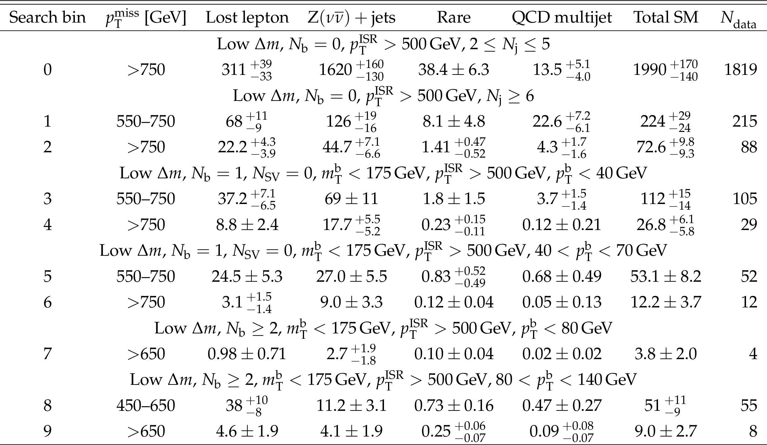
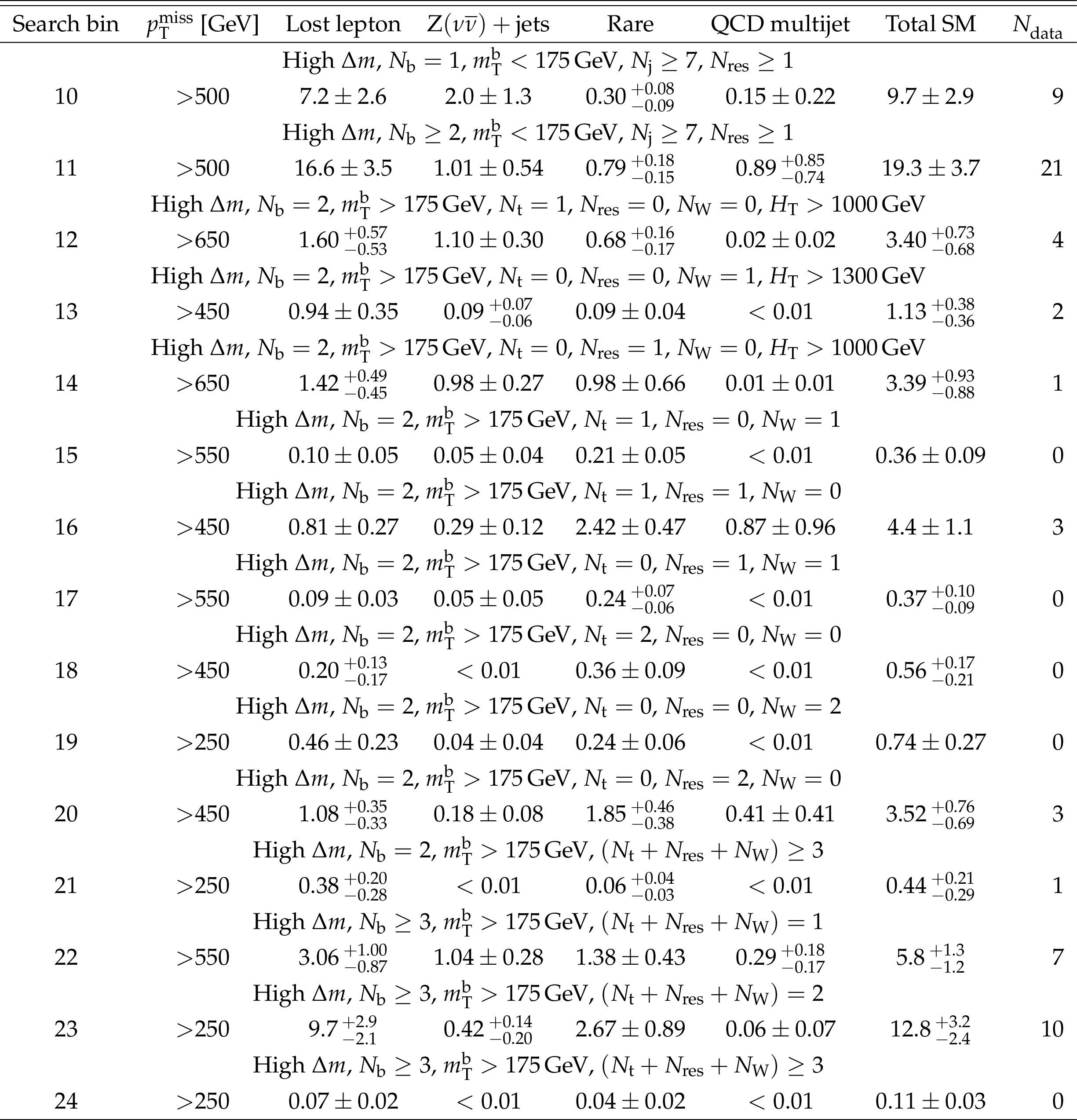
Table A1:
Observed number of events and SM background predictions in search bins 0-27. |
png pdf |
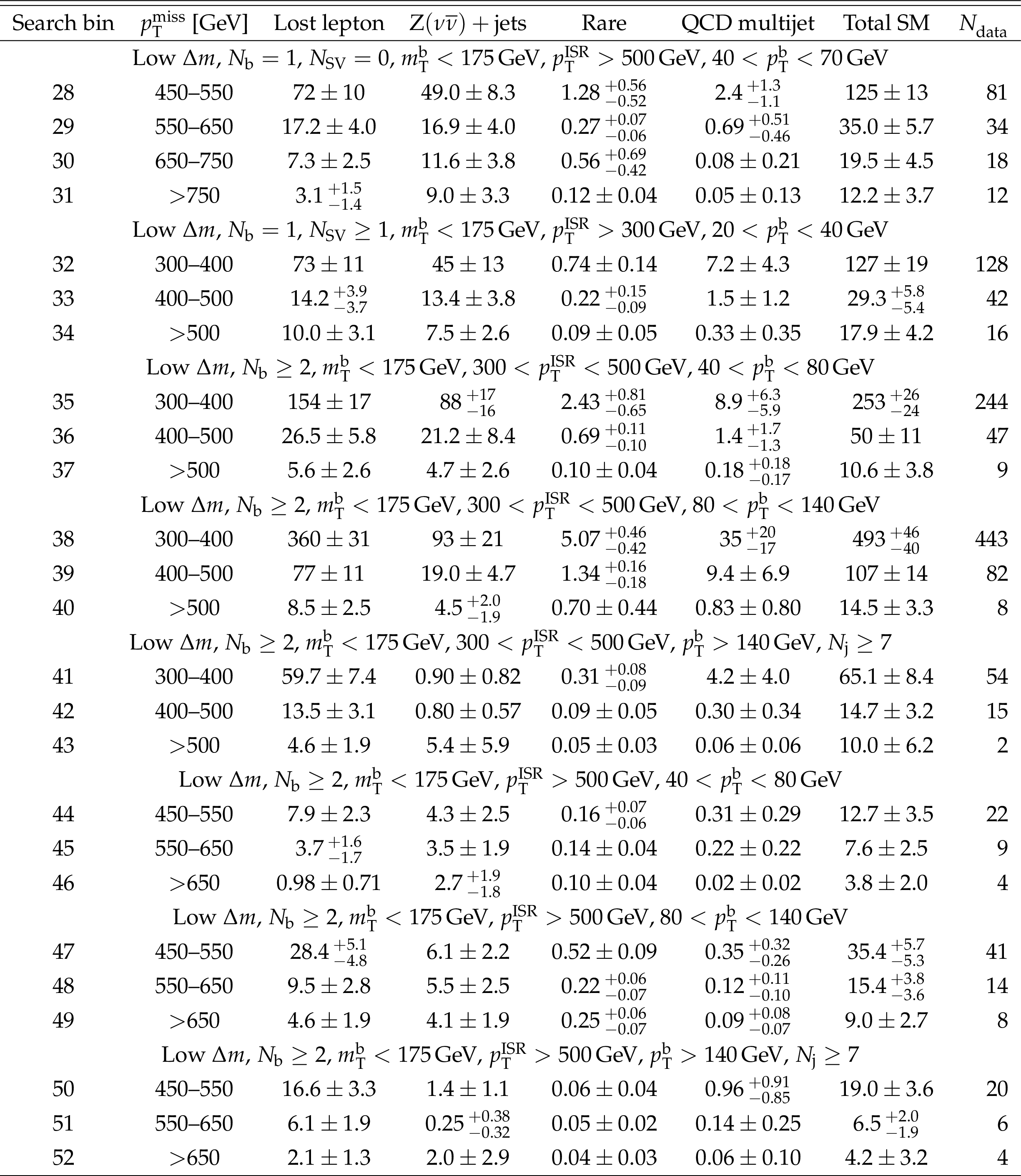
Table A2:
Observed number of events and SM background predictions in search bins 28-52. |

png pdf |
Table A3:
Observed number of events and SM background predictions in search bins 53-80. |

png pdf |
Table A4:
Observed number of events and SM background predictions in search bins 81-107. |
png pdf |
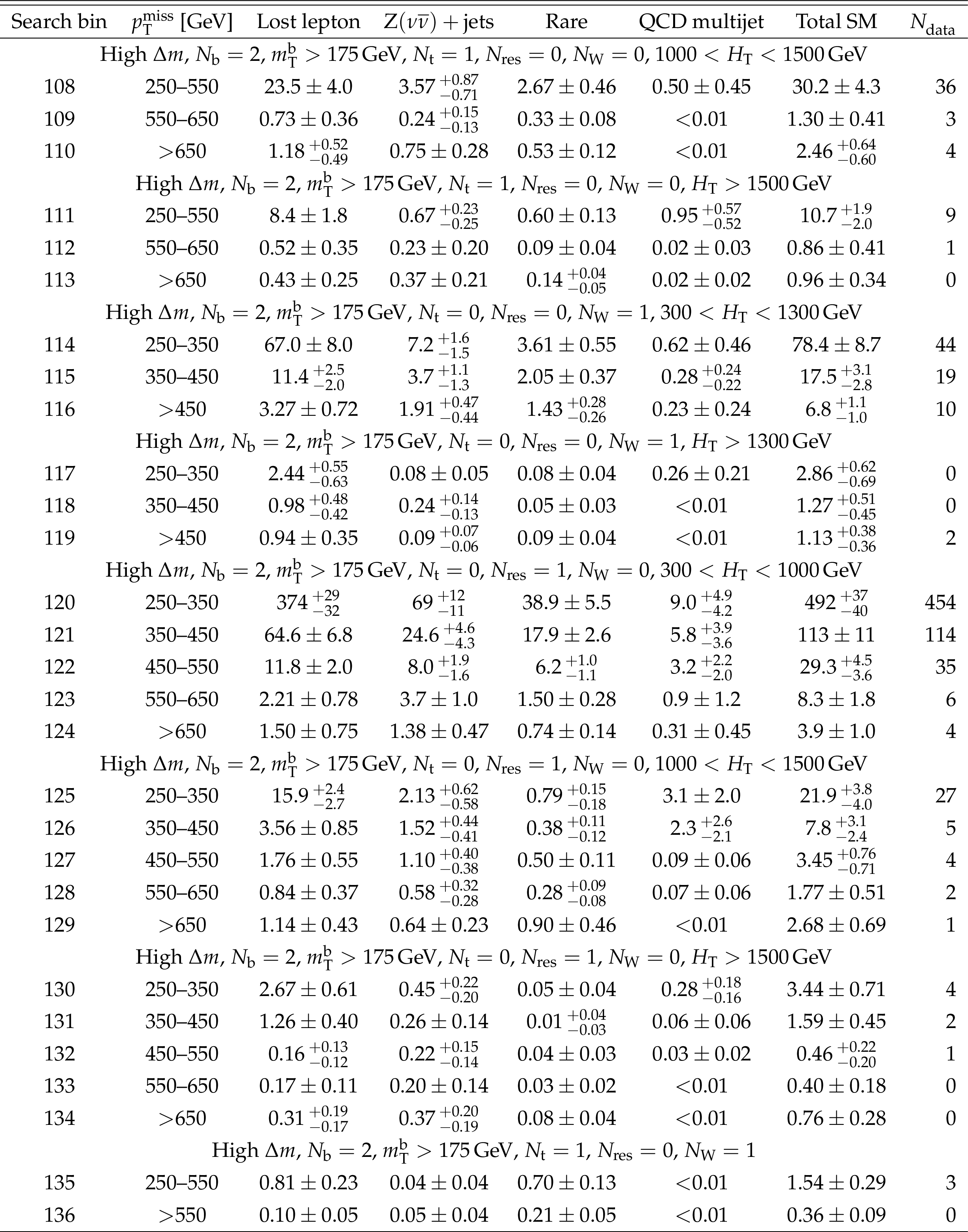
Table A5:
Observed number of events and SM background predictions in search bins 108-136. |
png pdf |
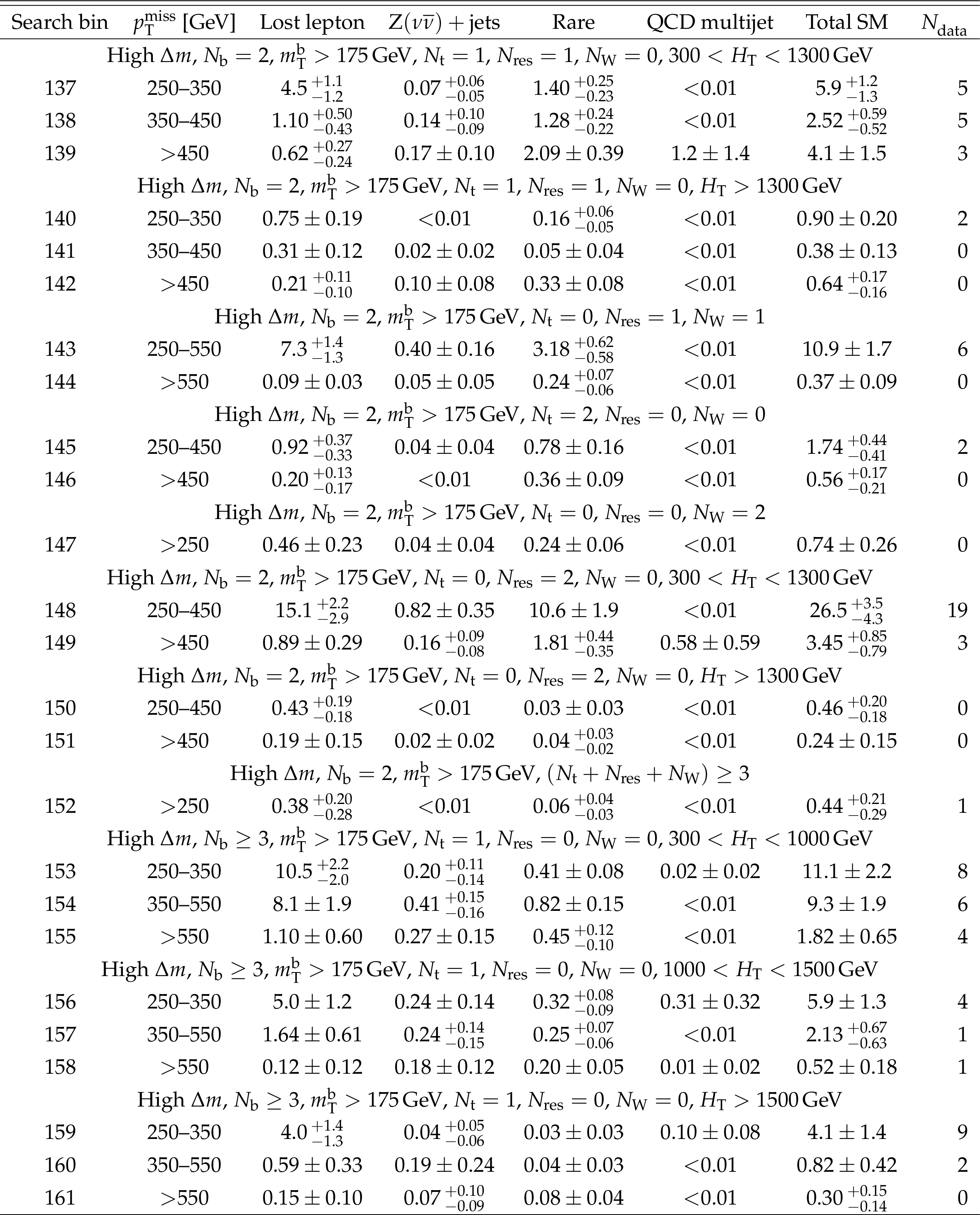
Table A6:
Observed number of events and SM background predictions in search bins 137-161. |
png pdf |
Table A7:
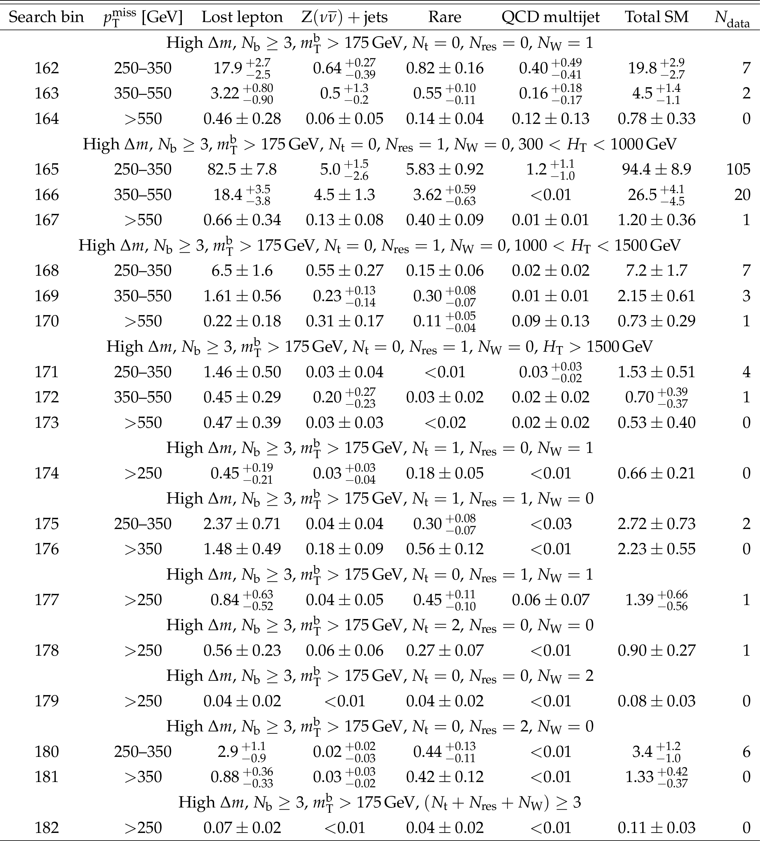
Observed number of events and SM background predictions in search bins 162-182. |
| Summary |
|
Results are presented from a search for direct and gluino-mediated top squark production in proton-proton collisions at a center-of-mass energy of 13 TeV. The analysis includes deep neural network based tagging algorithms for top quarks and W bosons both at low and high transverse momentum. The search is based on events with at least two jets and large imbalance in transverse momentum ${p_{\mathrm{T}}^{\text{miss}}}$. The data set corresponds to an integrated luminosity of 137 fb$^{-1}$ collected with the CMS detector at the LHC in 2016-2018. A set of 183 search bins is defined based on several kinematic variables and the number of reconstructed top quarks, bottom quarks, and W bosons. No statistically significant excess of events is observed with respect to the expectation from the standard model. Upper limits at the 95% confidence level are established on the cross section for several simplified models of direct and gluino-mediated top squark pair production as a function of the masses of the supersymmetric particles. Using the predicted cross sections, which are calculated with approximate next-to-next-to-leading order plus next-to-next-to-leading logarithmic accuracy, lower limits at the 95% confidence level are established on the top squark, lightest supersymmetric particle (LSP), and gluino masses. In the case of the direct top squark production models, top squark masses are excluded below a limit ranging from 1150 to 1310 GeV in the region of parameter space where the mass difference between the top squark and the LSP is larger than the W boson mass, depending on the top squark decay scenario. In the region of parameter space where the mass difference between the top squark and the LSP is smaller than the mass of the W boson, top squark masses are excluded below a limit ranging from 630 to 740 GeV, depending on the top squark decay scenario. In the case of the gluino-mediated top squark production models, gluino masses are excluded below a limit ranging from 2150 to 2260 GeV, depending on the signal model. These results significantly extend the mass exclusions of the previous top squark searches in the fully-hadronic final state from CMS [40,41] by about 100-300 GeV, benefiting not only from the larger data set, but also from improved analysis methods. For models of direct top squark production, the results obtained in this analysis are the most stringent constraints to date, regardless of the final state. |
| Additional Figures | |
png pdf |
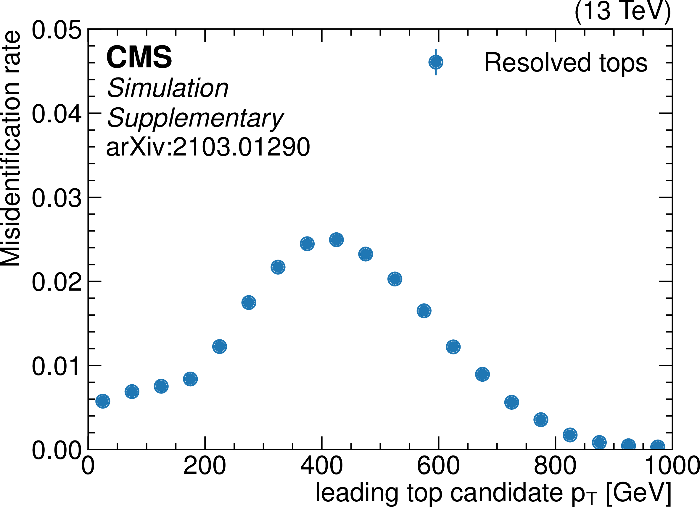
Additional Figure 1:
The misidentification rate for the DeepResolved top quark tagger is shown as a function of the ${p_{\mathrm {T}}}$ of the top quark candidate with the highest ${p_{\mathrm {T}}}$. A top quark candidate is defined as a trijet combination which satisfies the preselection requirements on the trijet mass (100 to 250 GeV), the maximum angle (no jet is farther than 3.1 from the trijet centroid in $\Delta R$), and the ${p_{\mathrm {T}}}$ of each of the three jets ($ {p_{\mathrm {T}}} > $ 40, 30, and 20 GeV, respectively). Top quark candidates must also survive the cross-cleaning process, which removes overlaps with tagged AK8 jets and other trijet candidates with lower NN discriminator scores. The misidentification rate is calculated in a simulated sample of QCD multijet events with $ {H_{\mathrm {T}}} > $ 300 GeV and is defined as the fraction of the candidates which have an NN discriminator score greater than 0.92. |
png pdf |
Additional Figure 2:
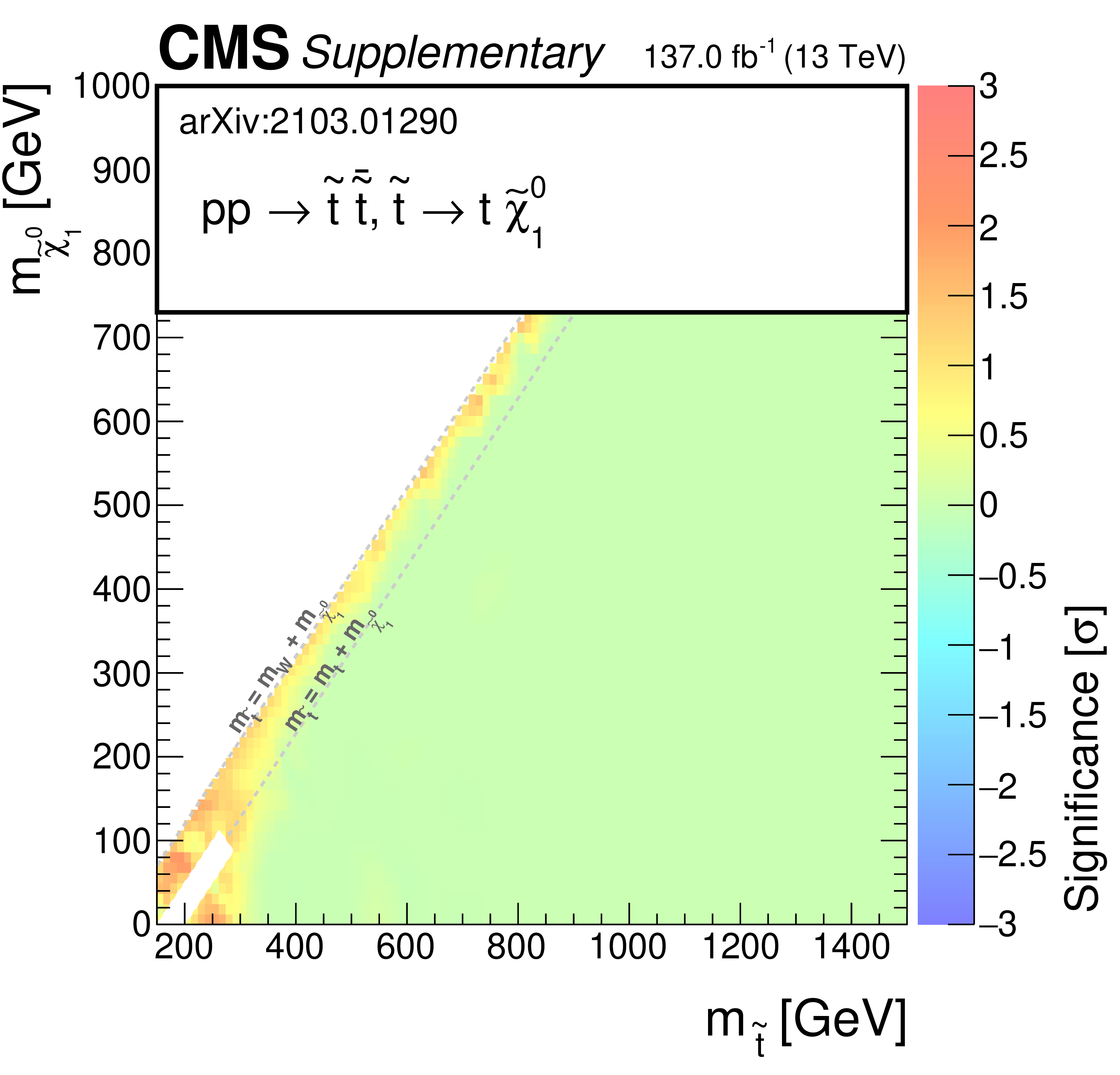
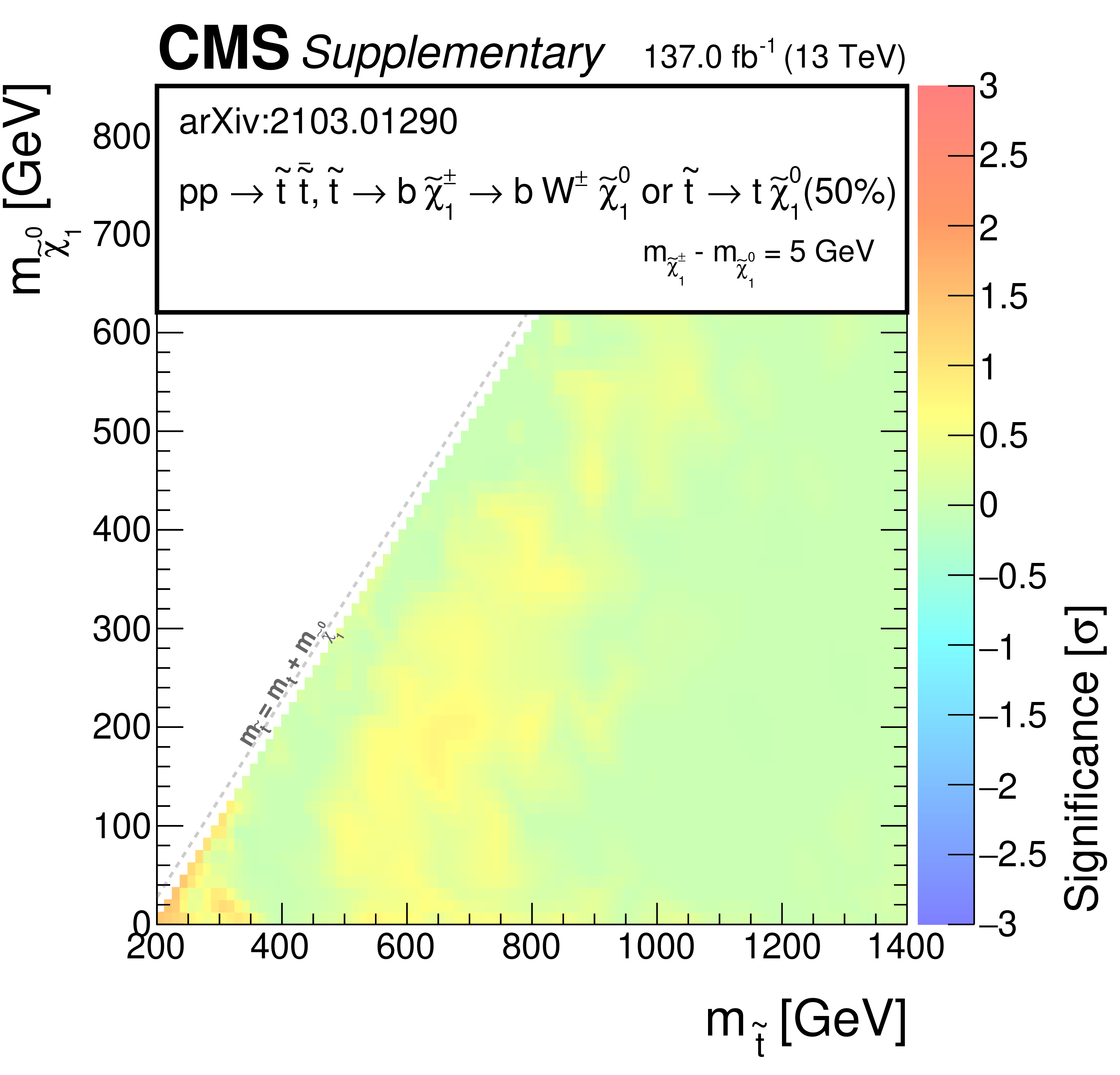
The observed significance of any excess in the data above the expected backgrounds, interpreted in the context of the SMS squark models for T2tt as a function of the top squark and LSP masses. |
png pdf |
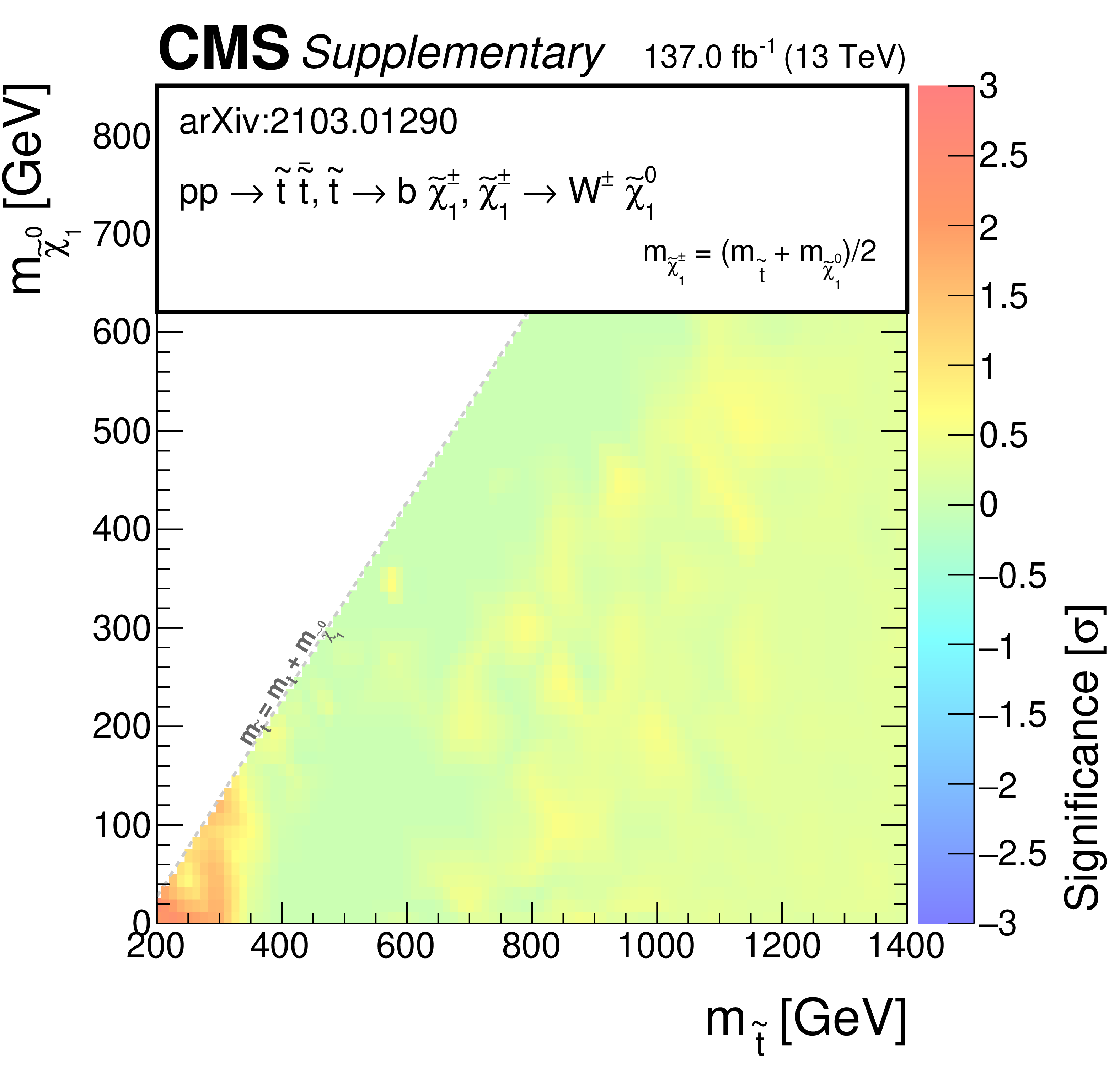
Additional Figure 3:
The observed significance of any excess in the data above the expected backgrounds, interpreted in the context of the SMS squark models for T2bW as a function of the top squark and LSP masses. |
png pdf |
Additional Figure 4:
The observed significance of any excess in the data above the expected backgrounds, interpreted in the context of the SMS squark models for T2tb as a function of the top squark and LSP masses. |
png pdf |
Additional Figure 5:
The observed significance of any excess in the data above the expected backgrounds, interpreted in the context of the SMS squark models for T2ttC as a function of the top squark mass and the difference between the top squark and LSP masses. |
png pdf |
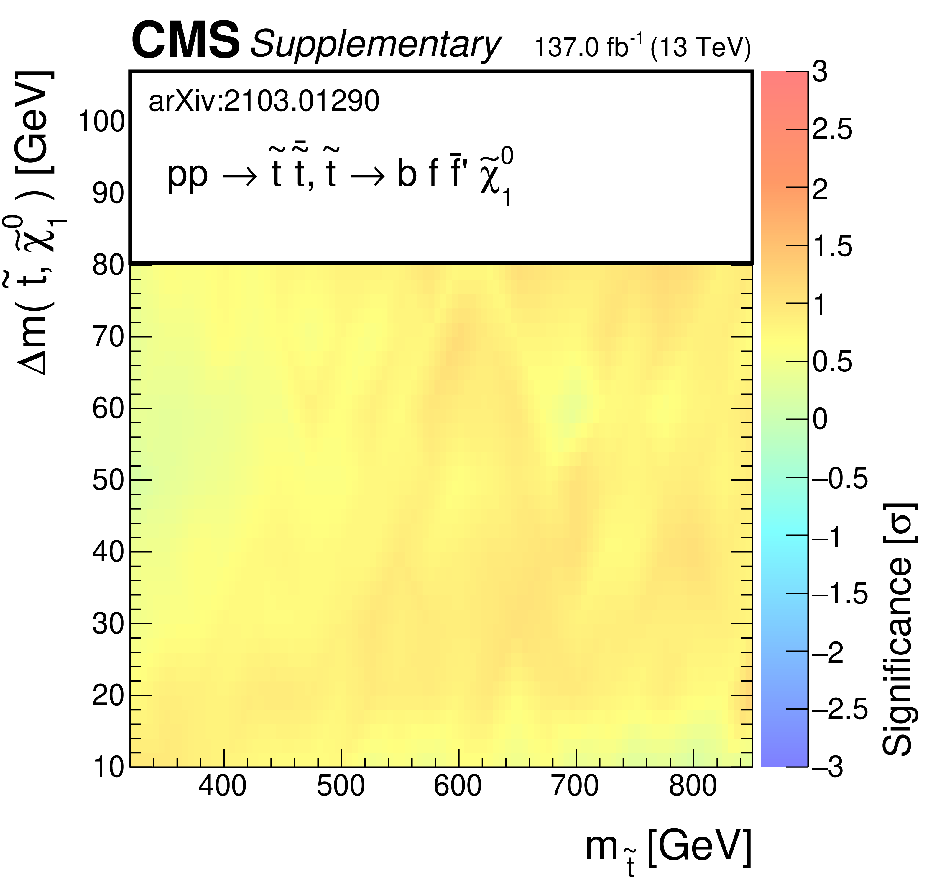
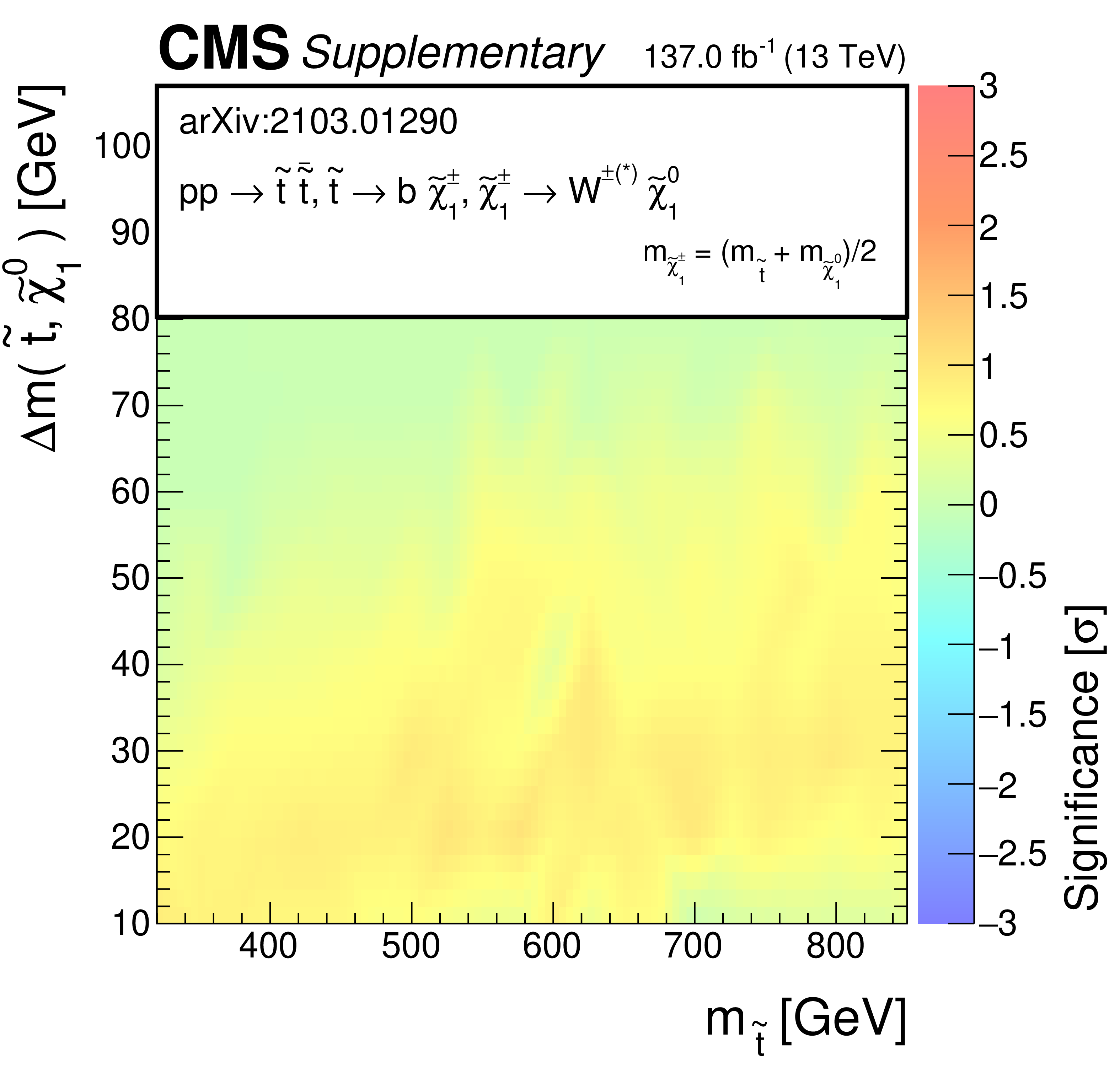
Additional Figure 6:
The observed significance of any excess in the data above the expected backgrounds, interpreted in the context of the SMS squark models for T2bWC as a function of the top squark mass and the difference between the top squark and LSP masses. |
png pdf |
Additional Figure 7:
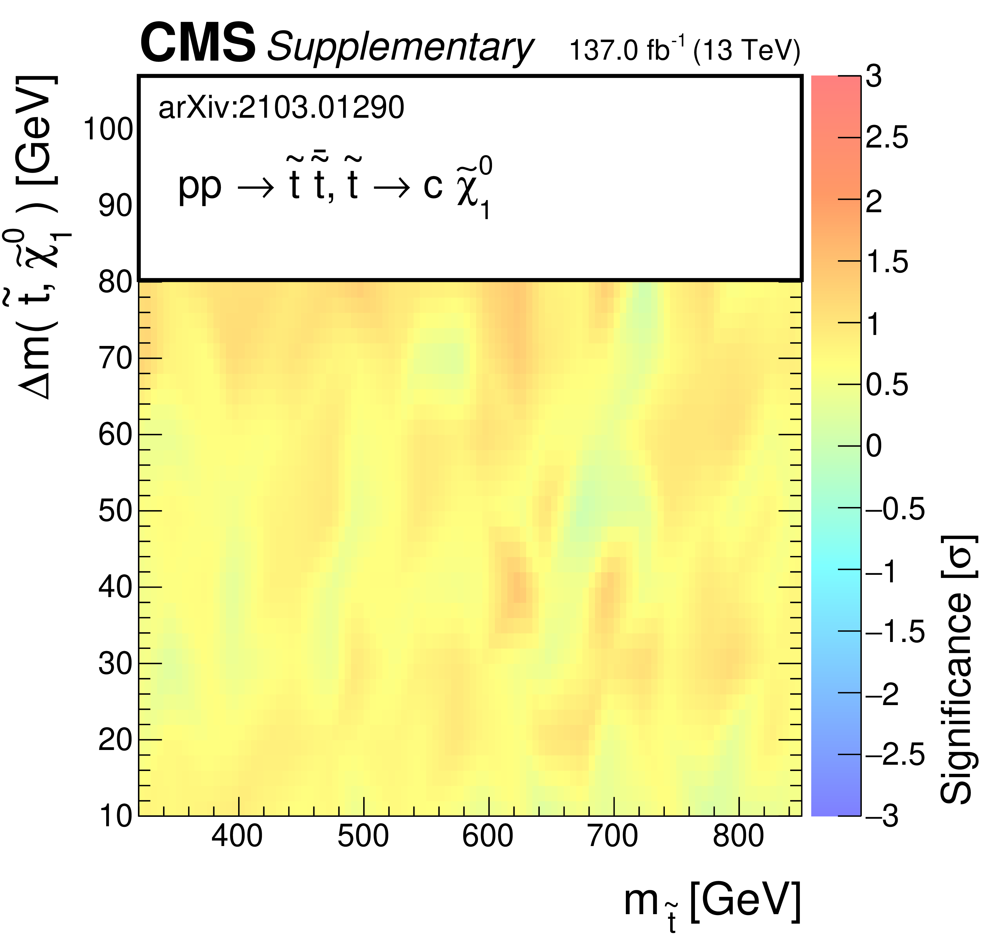
The observed significance of any excess in the data above the expected backgrounds, interpreted in the context of the SMS squark models for T2cc as a function of the top squark mass and the difference between the top squark and LSP masses. |
png pdf |
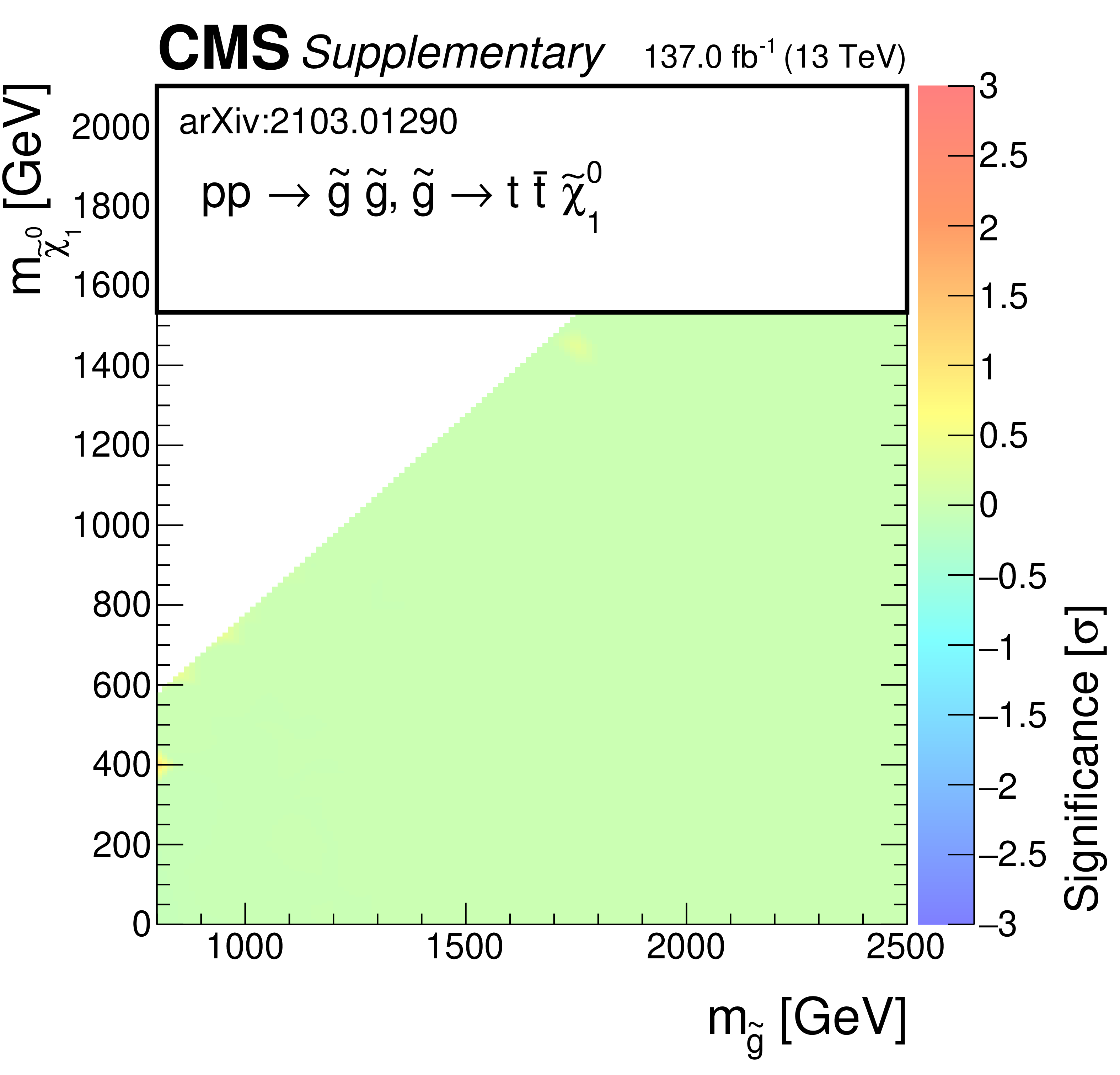
Additional Figure 8:
The observed significance of any excess in the data above the expected backgrounds, interpreted in the context of the SMS squark models for T1tttt as a function of the gluino and LSP masses. |
png pdf |
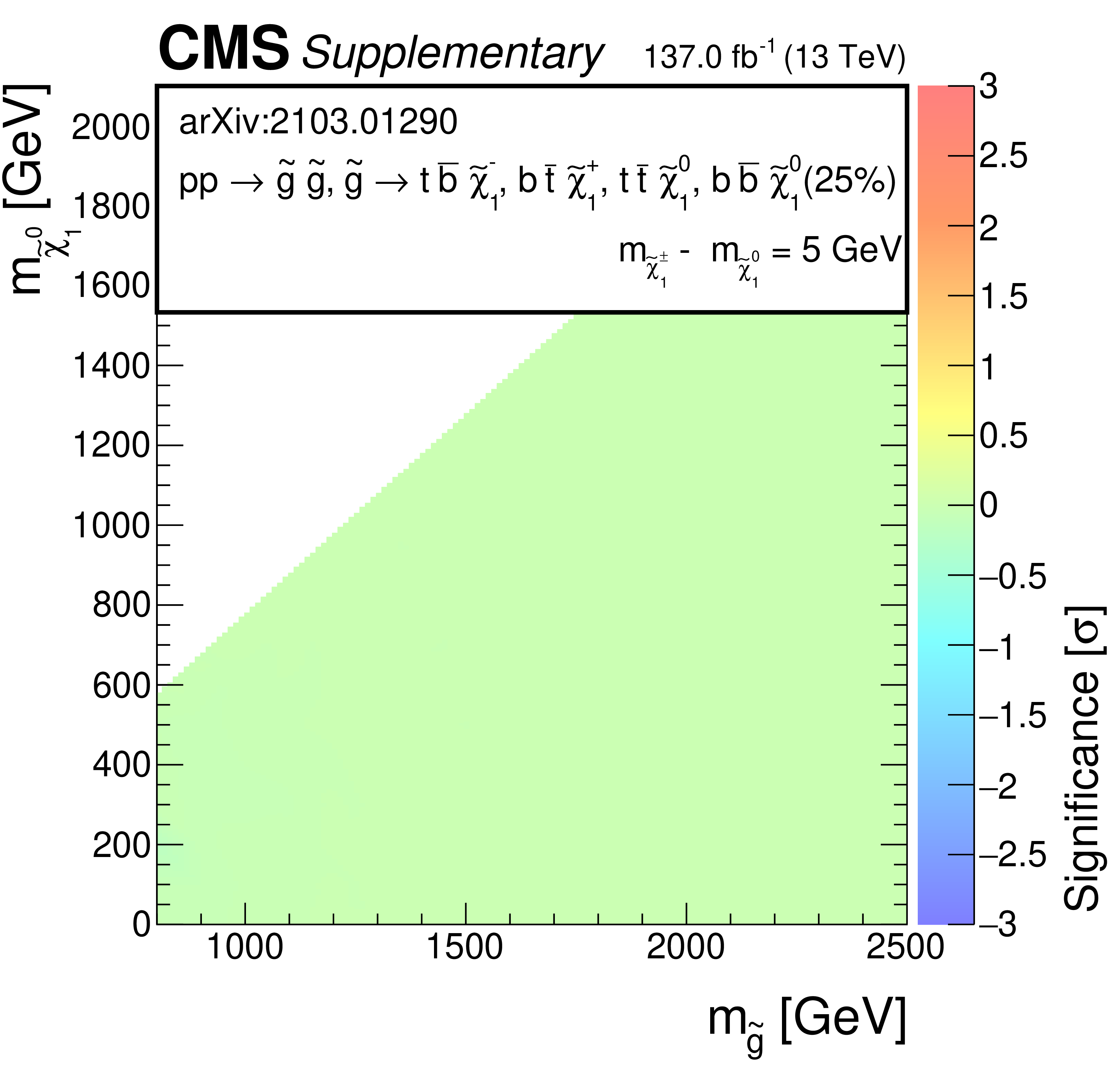
Additional Figure 9:
The observed significance of any excess in the data above the expected backgrounds, interpreted in the context of the SMS squark models for T1ttbb as a function of the gluino and LSP masses. |
png pdf |
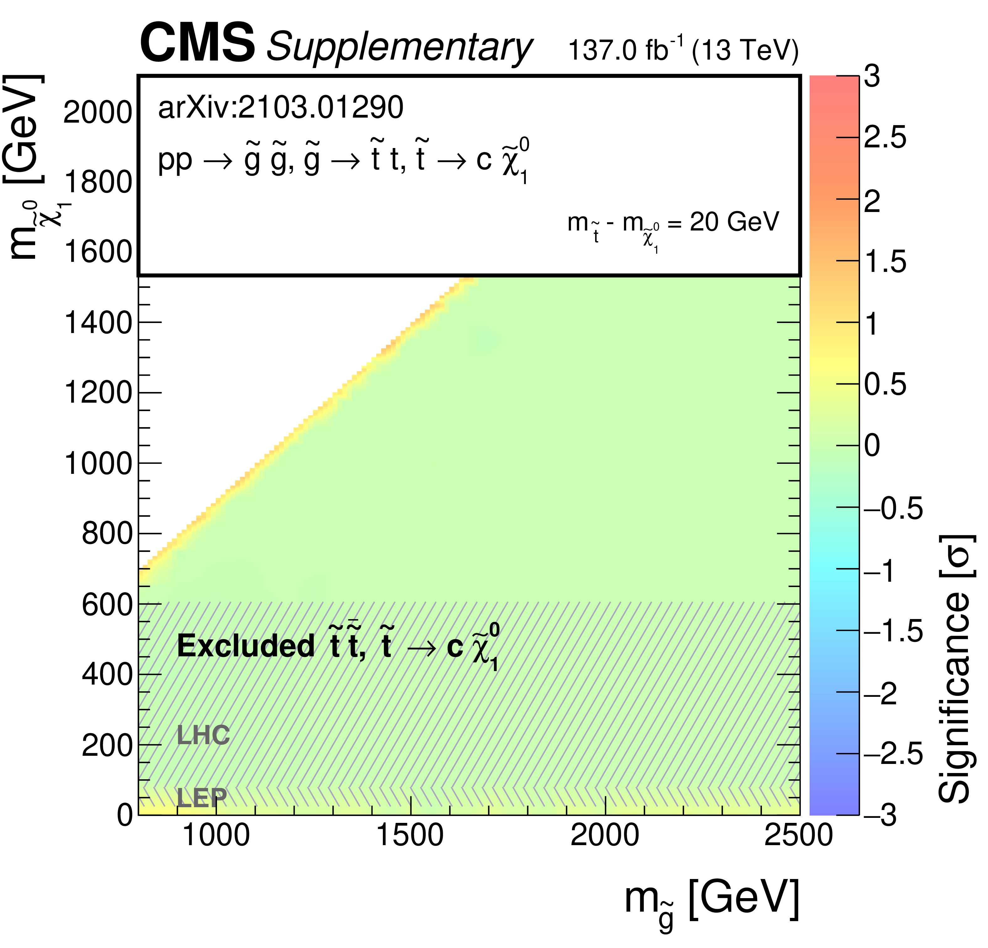
Additional Figure 10:
The observed significance of any excess in the data above the expected backgrounds, interpreted in the context of the SMS squark models for T5ttcc as a function of the gluino and LSP masses. Excluded regions based on direct top squark pair production from this search and earlier searches by the ATLAS, CMS, and LEP experiments are indicated by the hatched areas. |
png pdf |
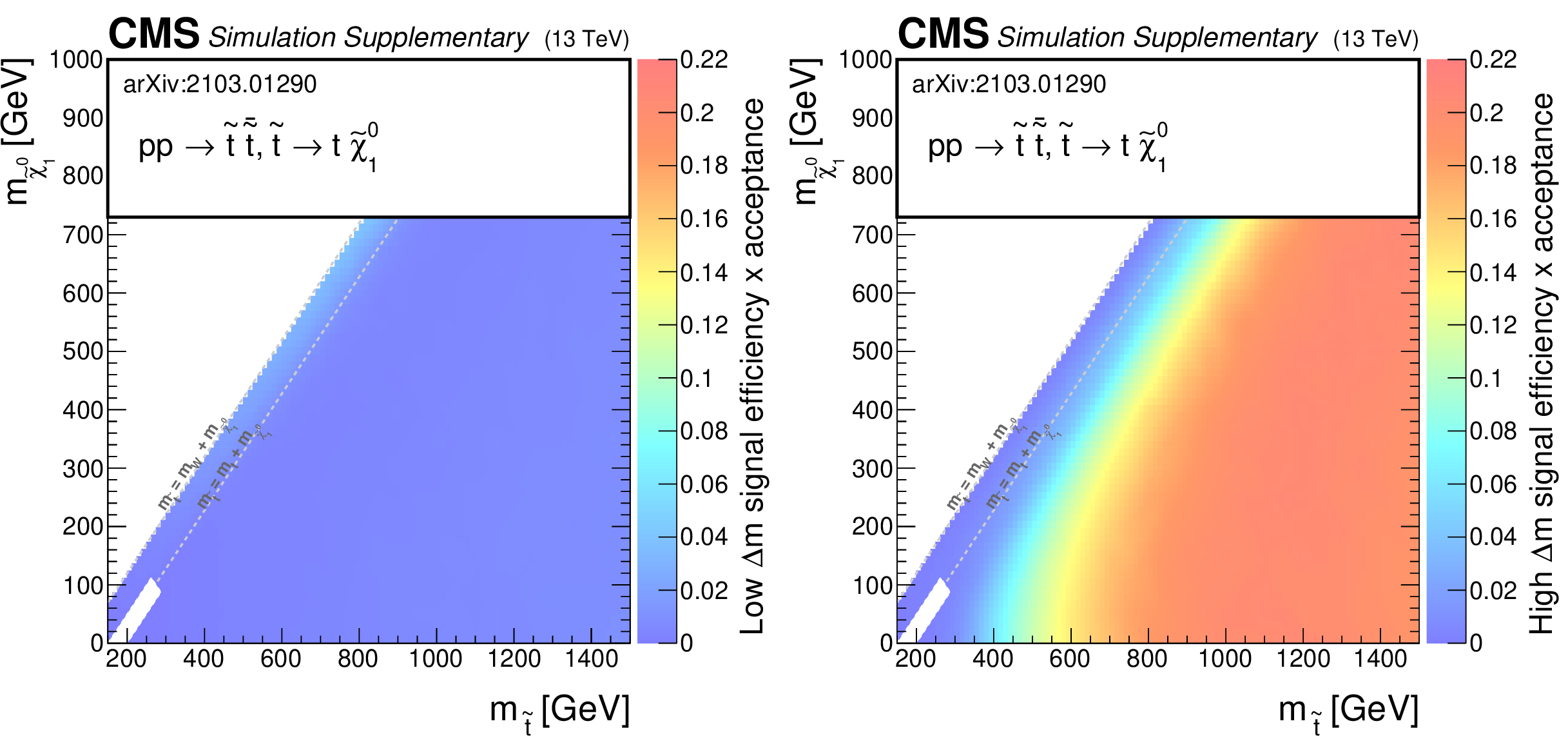
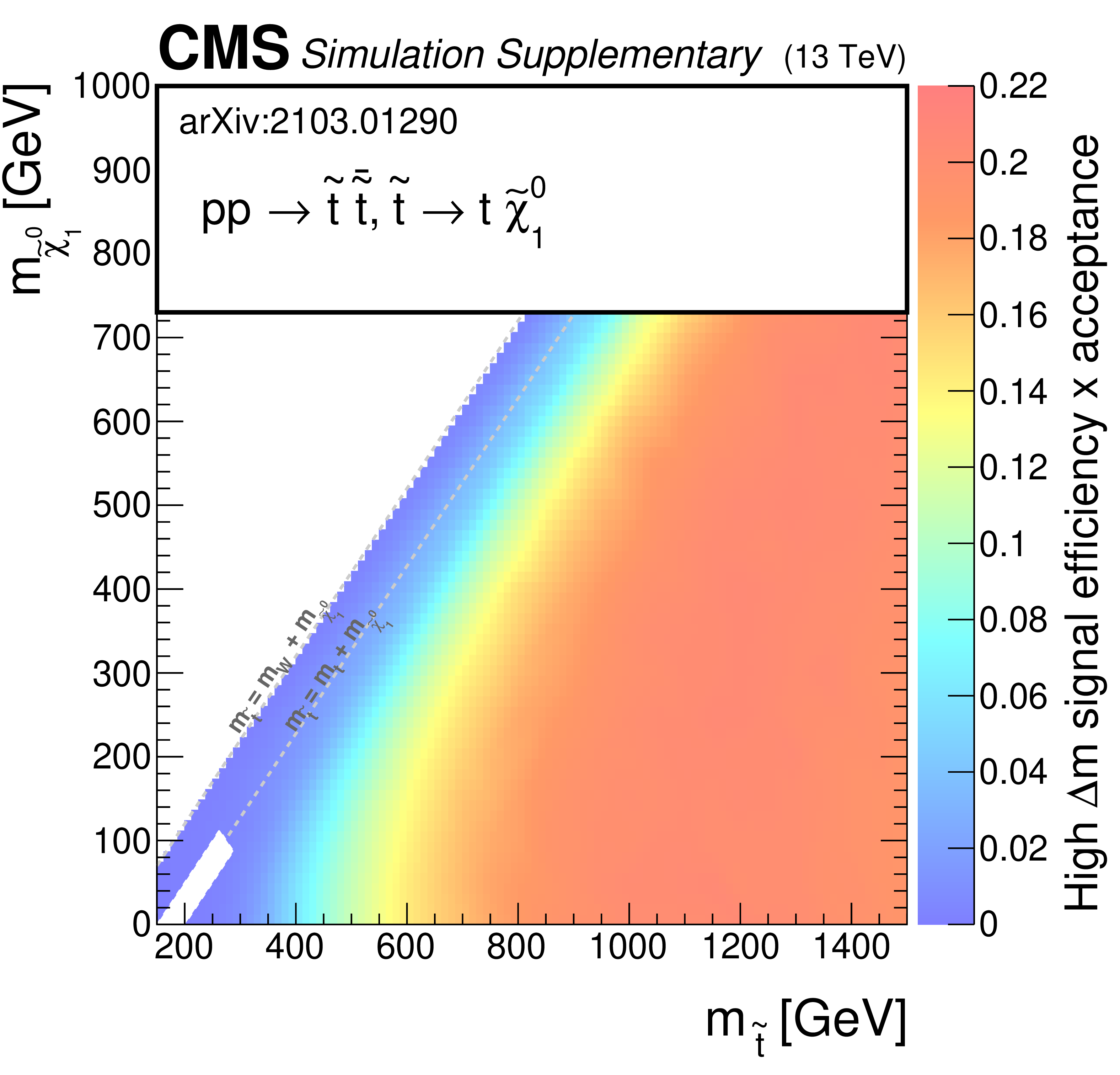
Additional Figure 11:
The efficiency times acceptance of the SMS squark models for T2tt as a function of the top squark and LSP masses in the union of the 53 low ${\Delta m}$ search regions (left) and the 130 high ${\Delta m}$ search regions (right). |

png pdf |
Additional Figure 11-a:
The efficiency times acceptance of the SMS squark models for T2tt as a function of the top squark and LSP masses in the union of the 53 low ${\Delta m}$ search regions. |
png pdf |
Additional Figure 11-b:
The efficiency times acceptance of the SMS squark models for T2tt as a function of the top squark and LSP masses in the union of the 130 high ${\Delta m}$ search regions. |

png pdf |
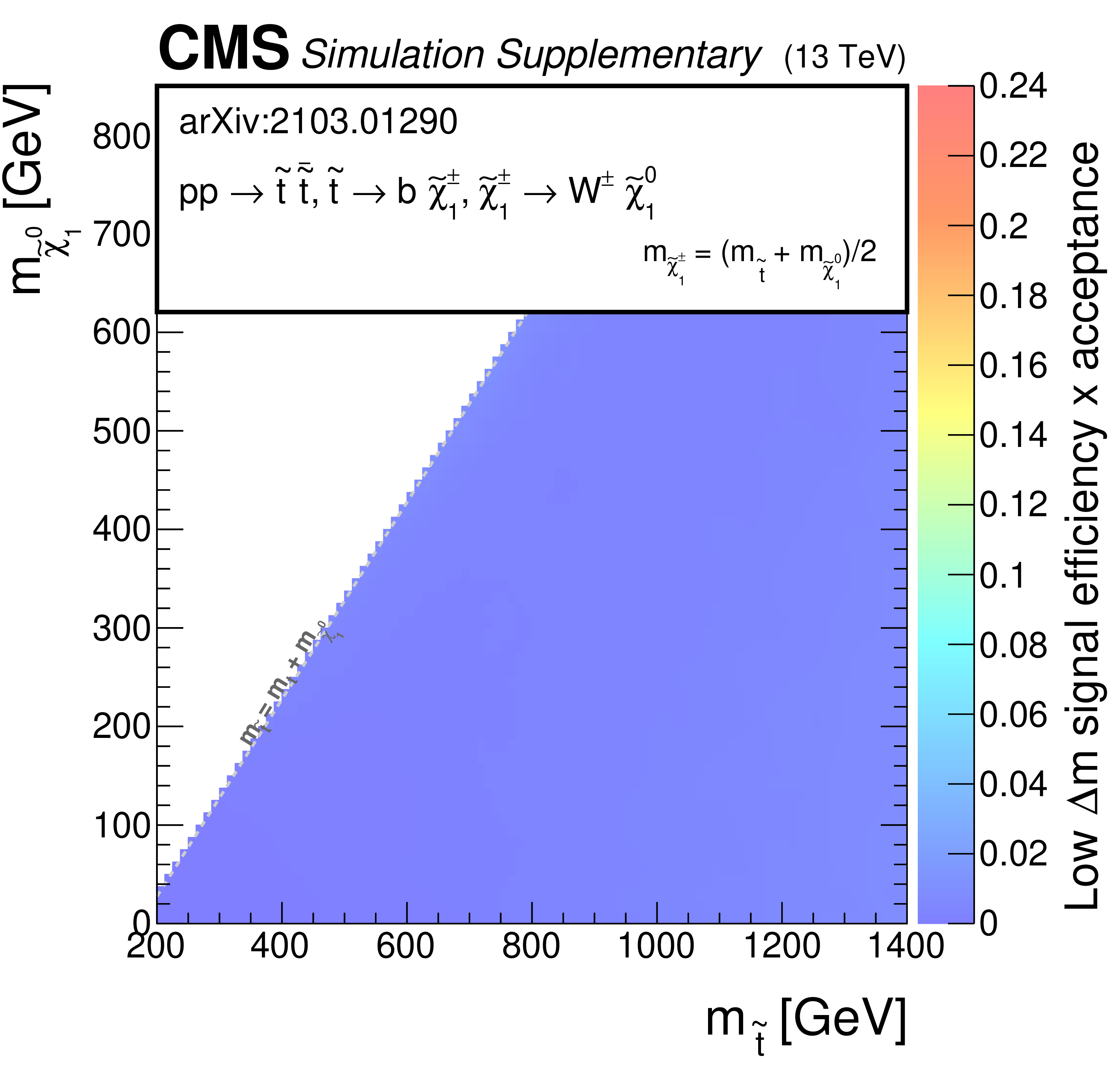
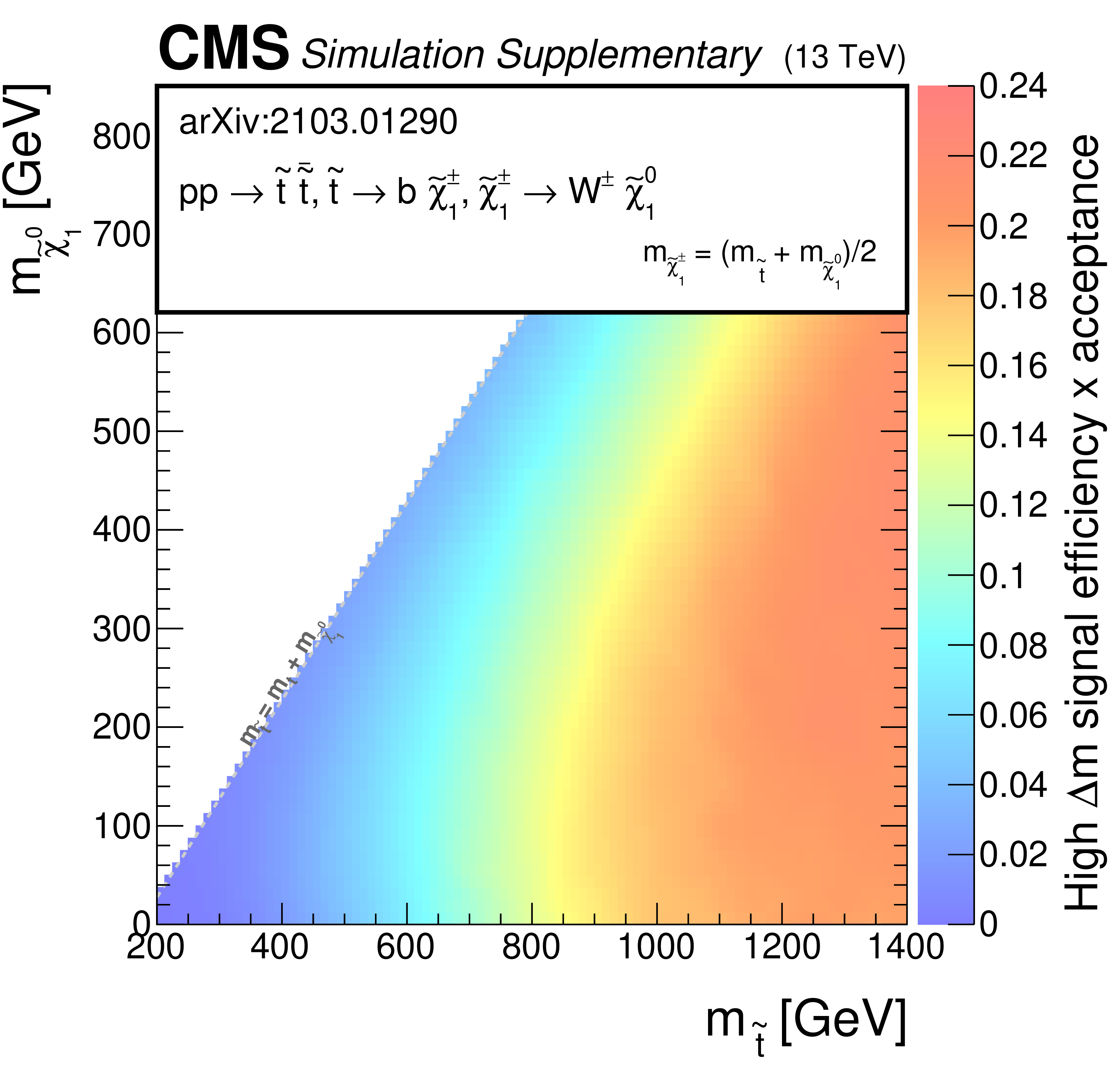
Additional Figure 12:
The efficiency times acceptance of the SMS squark models for T2bW as a function of the top squark and LSP masses in the union of the 53 low ${\Delta m}$ search regions (left) and the 130 high ${\Delta m}$ search regions (right). |
png pdf |
Additional Figure 12-a:
The efficiency times acceptance of the SMS squark models for T2bW as a function of the top squark and LSP masses in the union of the 53 low ${\Delta m}$ search regions. |
png pdf |
Additional Figure 12-b:
The efficiency times acceptance of the SMS squark models for T2bW as a function of the top squark and LSP masses in the union of the 130 high ${\Delta m}$ search regions. |

png pdf |
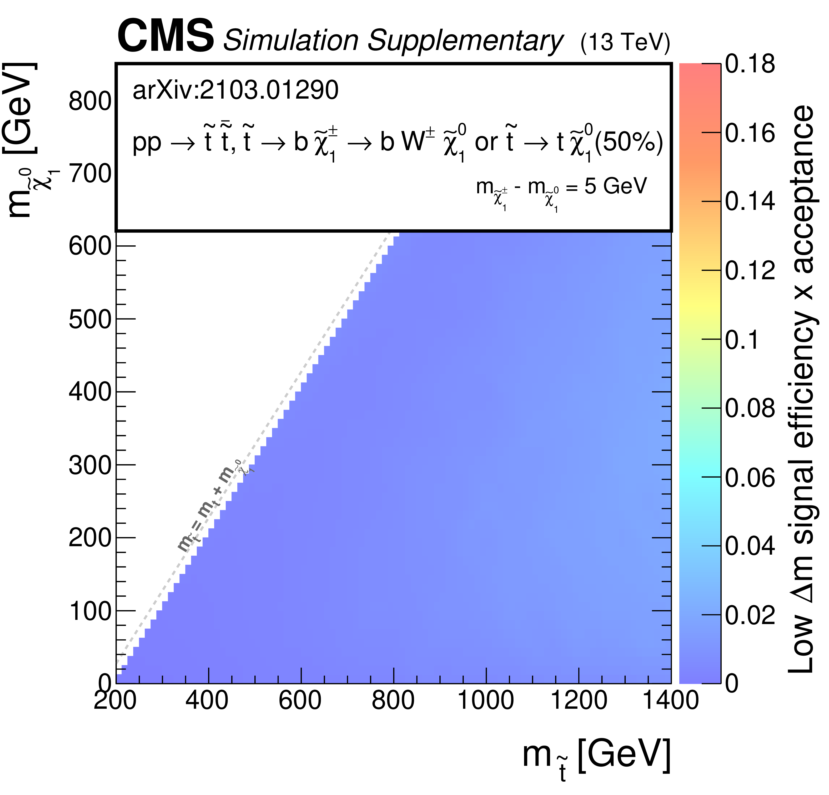
Additional Figure 13:
The efficiency times acceptance of the SMS squark models for T2tb as a function of the top squark and LSP masses in the union of the 53 low ${\Delta m}$ search regions (left) and the 130 high ${\Delta m}$ search regions (right). |
png pdf |
Additional Figure 13-a:
The efficiency times acceptance of the SMS squark models for T2tb as a function of the top squark and LSP masses in the union of the 53 low ${\Delta m}$ search regions. |

png pdf |
Additional Figure 13-b:
The efficiency times acceptance of the SMS squark models for T2tb as a function of the top squark and LSP masses in the union of the 130 high ${\Delta m}$ search regions. |
png pdf |
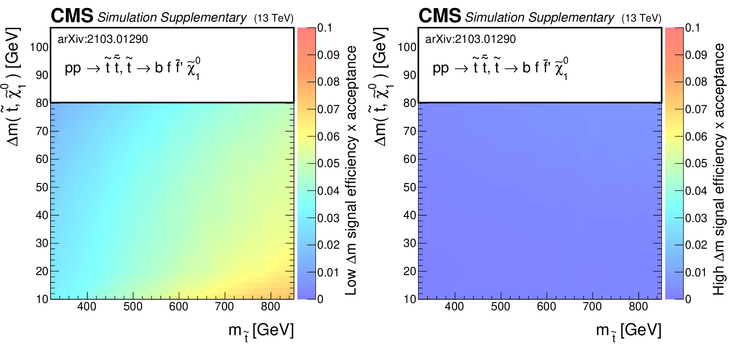
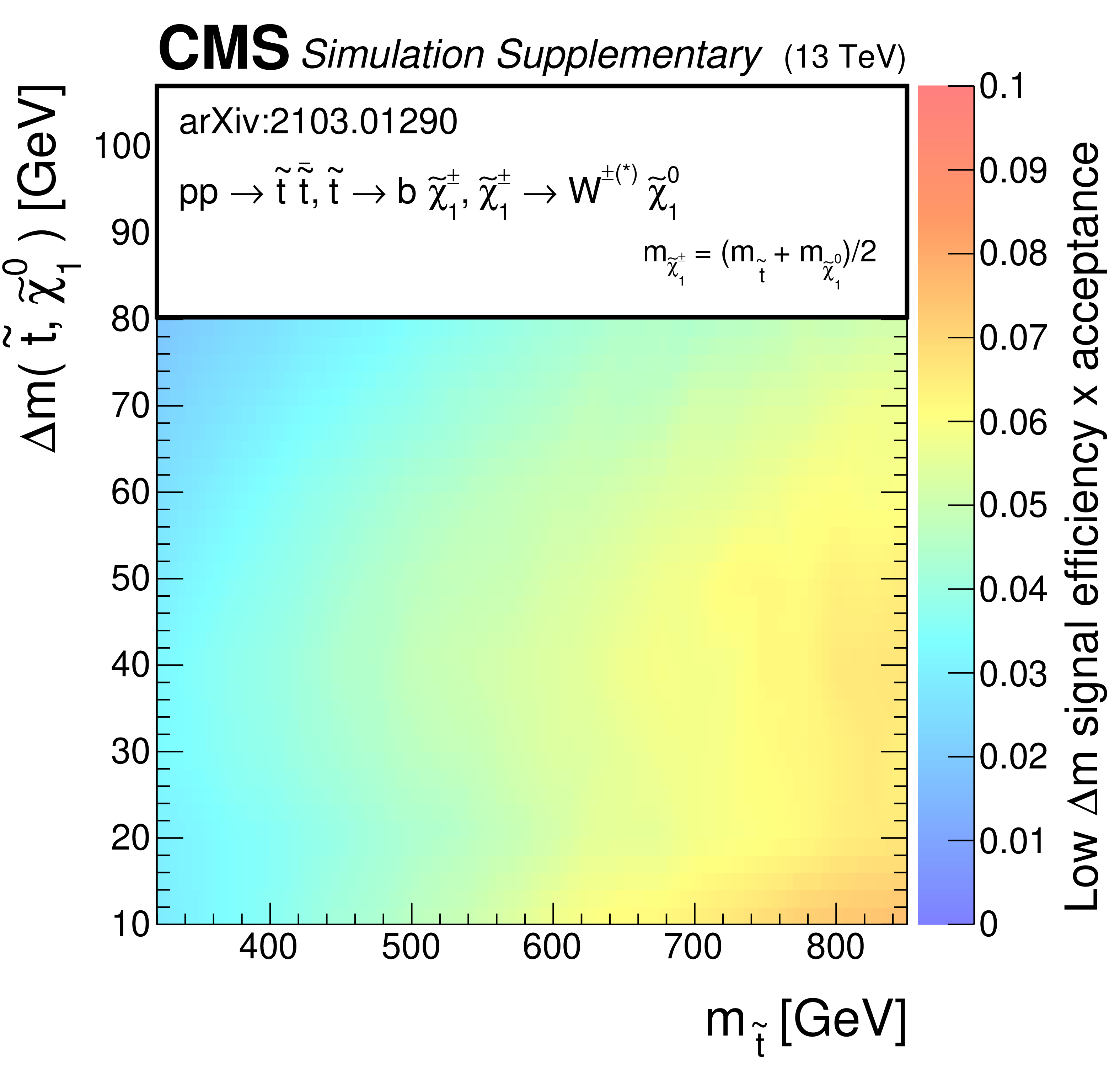
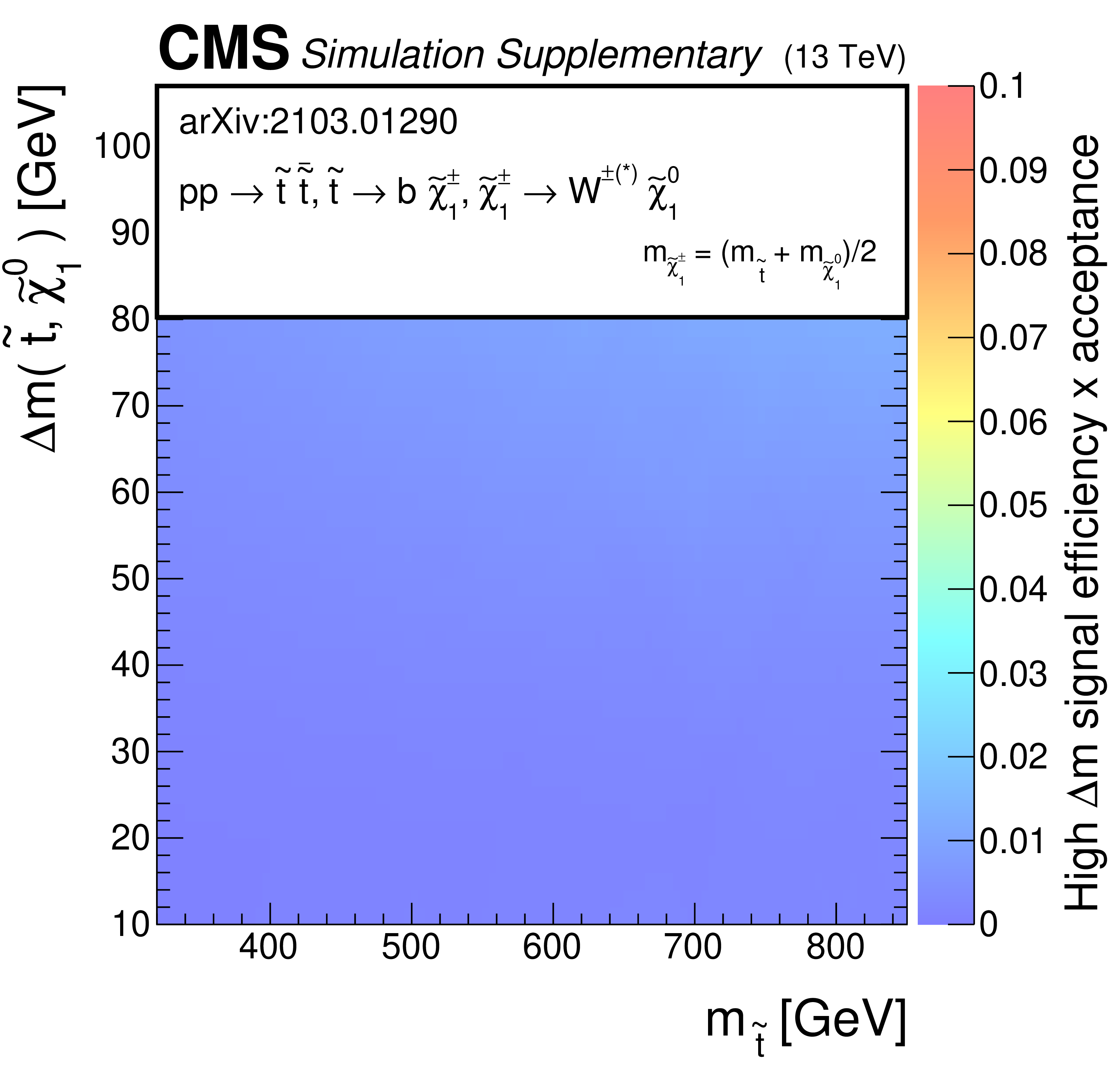
Additional Figure 14:
The efficiency times acceptance of the SMS squark models for T2ttC as a function of the top squark and the difference between the top squark and LSP masses in the union of the 53 low ${\Delta m}$ search regions (left) and the 130 high ${\Delta m}$ search regions (right). |
png pdf |
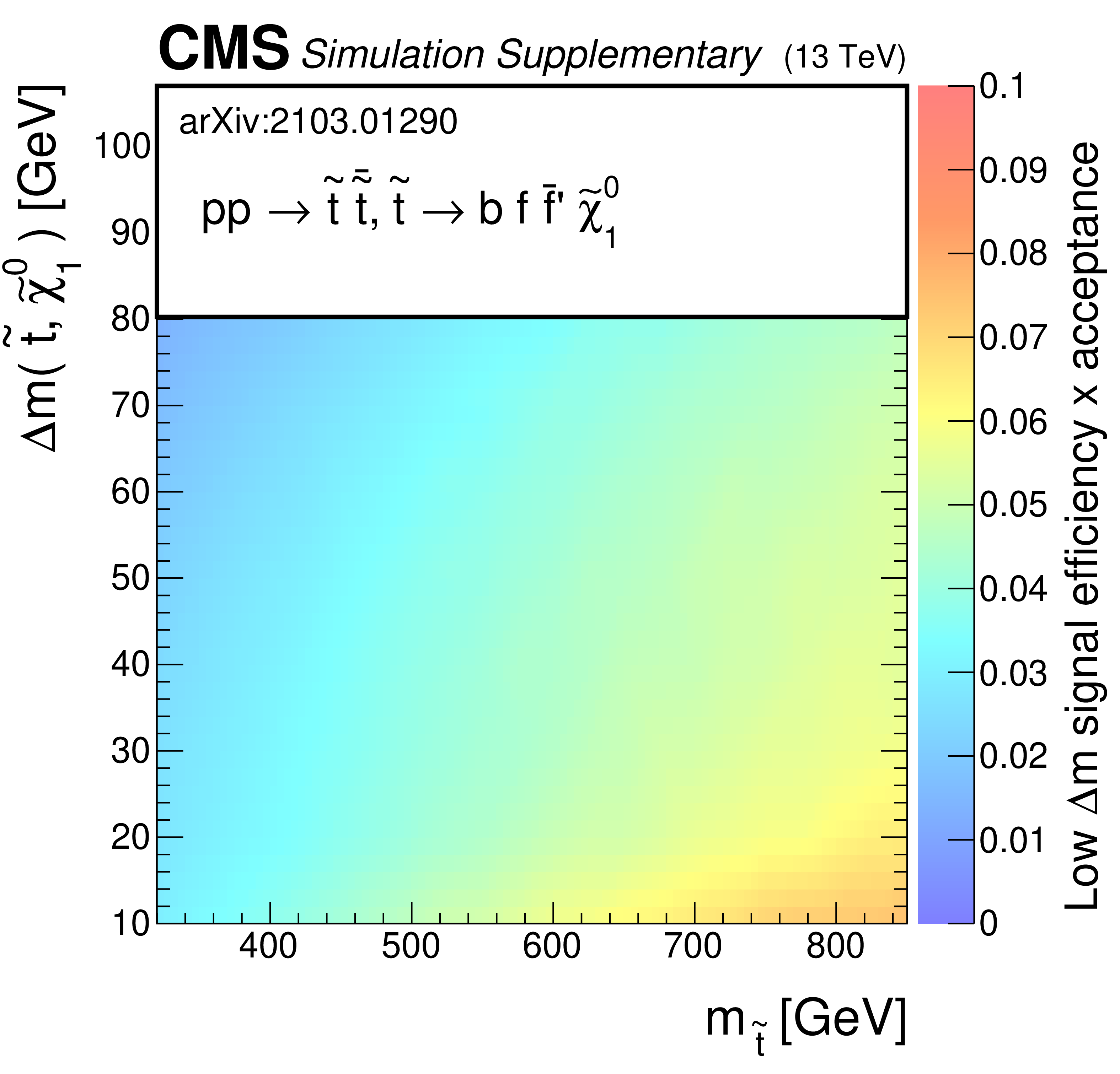
Additional Figure 14-a:
The efficiency times acceptance of the SMS squark models for T2ttC as a function of the top squark and the difference between the top squark and LSP masses in the union of the 53 low ${\Delta m}$ search regions. |
png pdf |
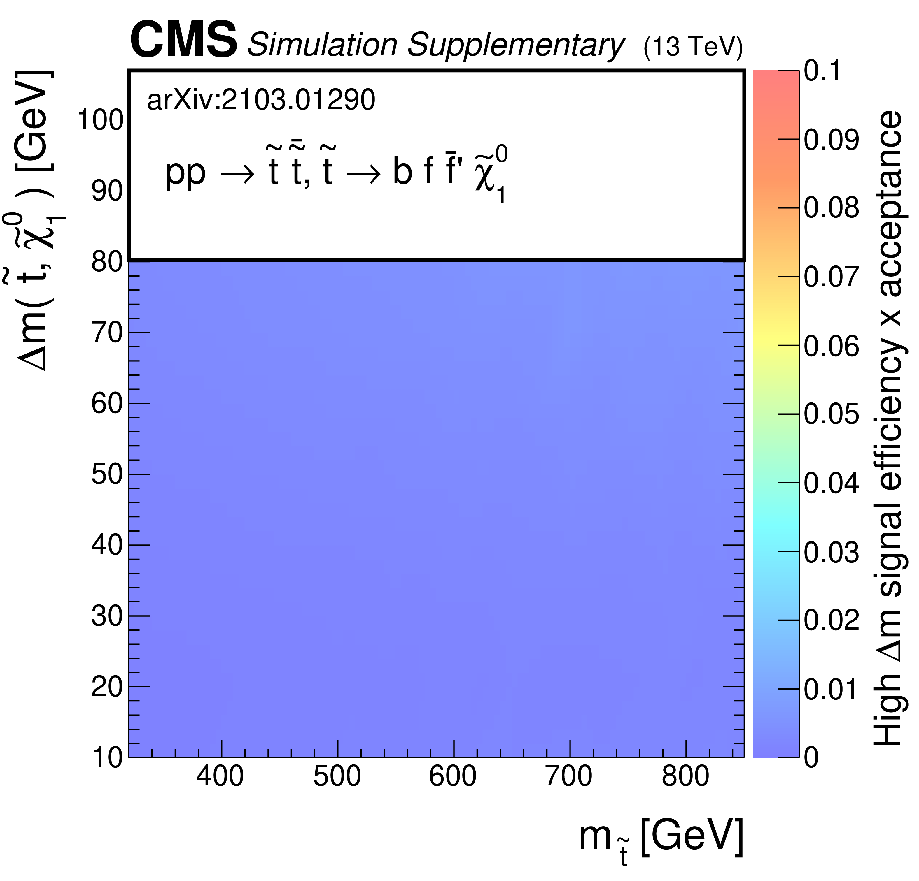
Additional Figure 14-b:
The efficiency times acceptance of the SMS squark models for T2ttC as a function of the top squark and the difference between the top squark and LSP masses in the union of the 130 high ${\Delta m}$ search regions. |
png pdf |
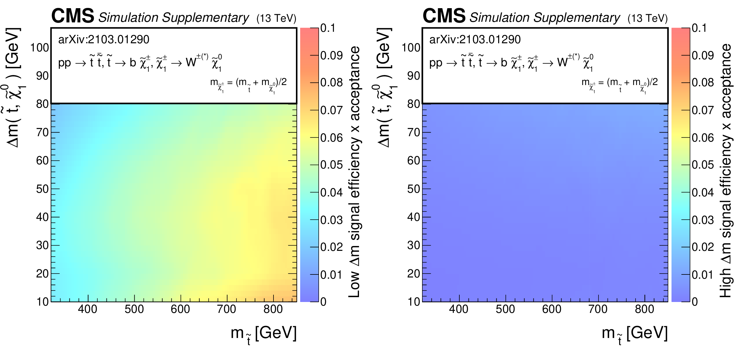
Additional Figure 15:
The efficiency times acceptance of the SMS squark models for T2bWC as a function of the top squark and the difference between the top squark and LSP masses in the union of the 53 low ${\Delta m}$ search regions (left) and the 130 high ${\Delta m}$ search regions (right). |
png pdf |
Additional Figure 15-a:
The efficiency times acceptance of the SMS squark models for T2bWC as a function of the top squark and the difference between the top squark and LSP masses in the union of the 53 low ${\Delta m}$ search regions. |
png pdf |
Additional Figure 15-b:
The efficiency times acceptance of the SMS squark models for T2bWC as a function of the top squark and the difference between the top squark and LSP masses in the union of the 130 high ${\Delta m}$ search regions. |
png pdf |
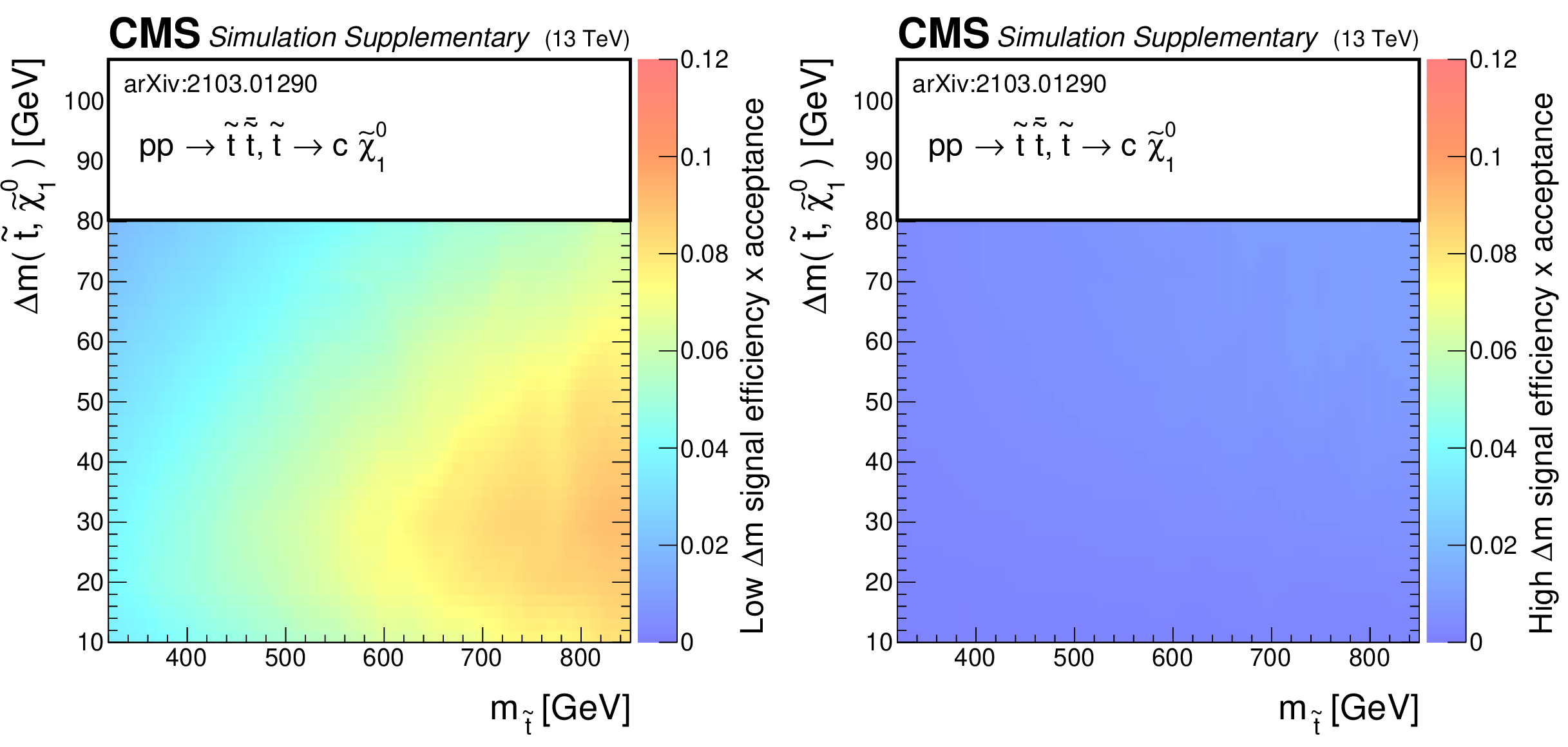
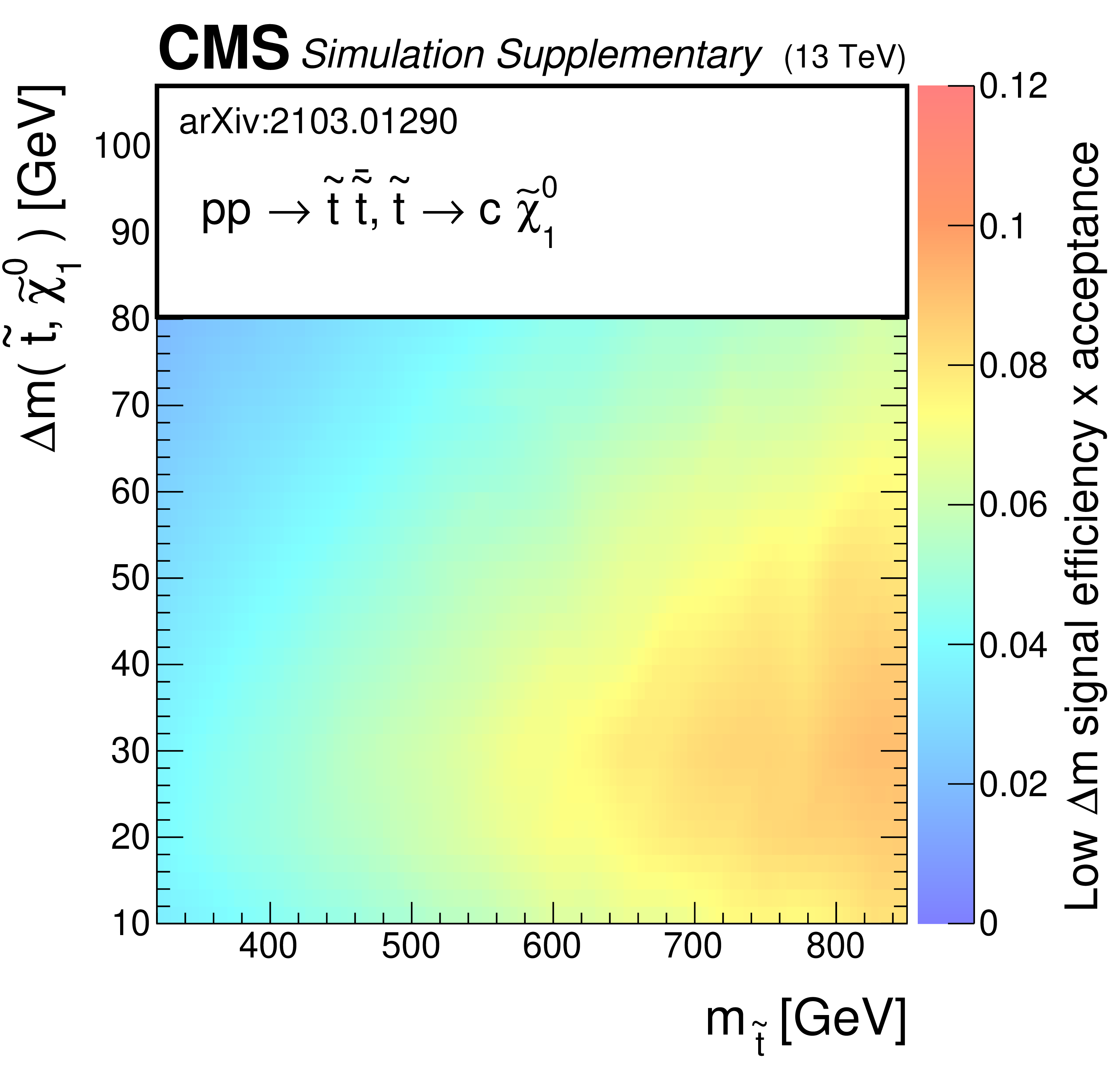
Additional Figure 16:
The efficiency times acceptance of the SMS squark models for T2cc as a function of the top squark and the difference between the top squark and LSP masses in the union of the 53 low ${\Delta m}$ search regions (left) and the 130 high ${\Delta m}$ search regions (right). |
png pdf |
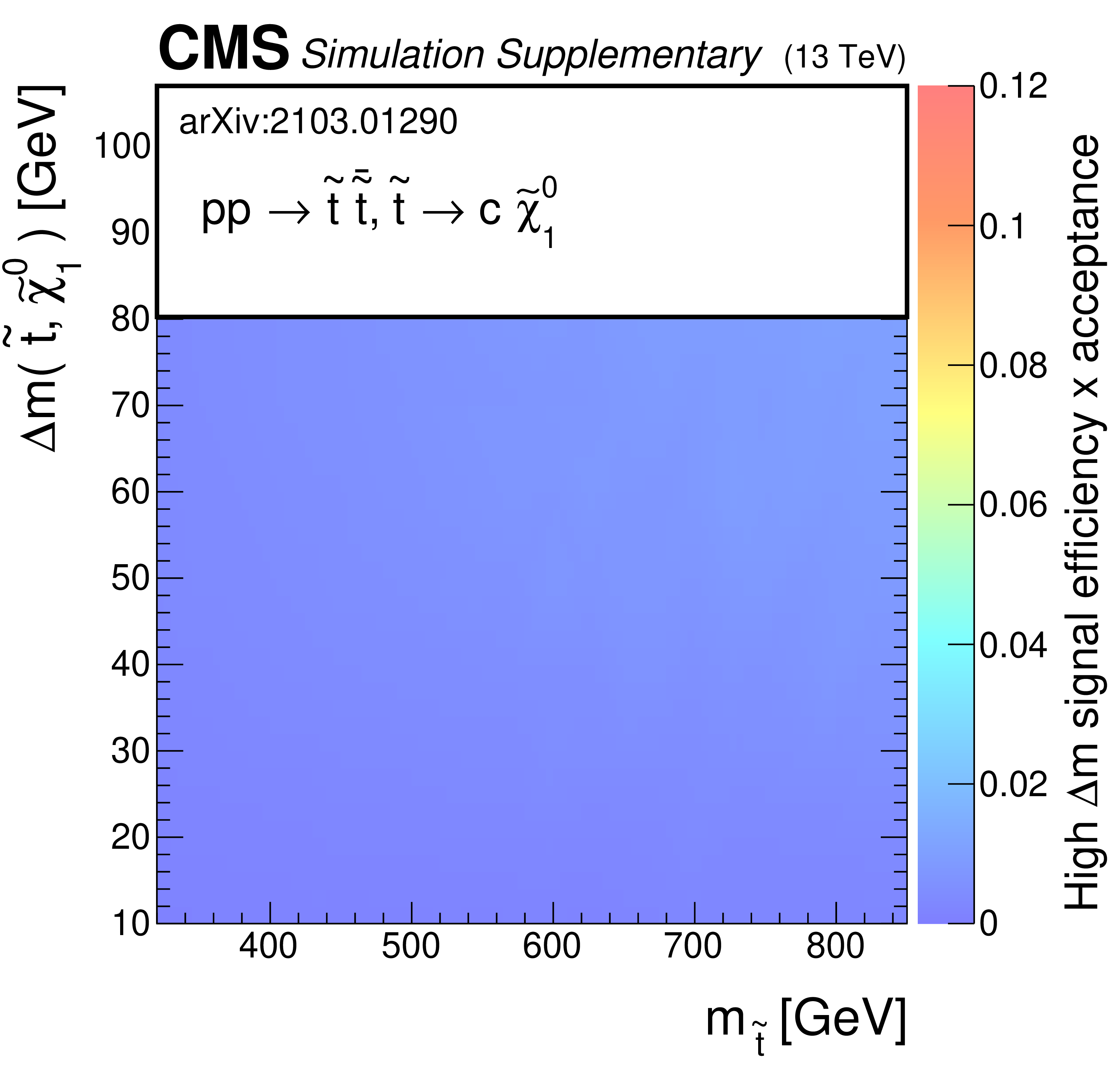
Additional Figure 16-a:
The efficiency times acceptance of the SMS squark models for T2cc as a function of the top squark and the difference between the top squark and LSP masses in the union of the 53 low ${\Delta m}$ search regions. |
png pdf |
Additional Figure 16-b:
The efficiency times acceptance of the SMS squark models for T2cc as a function of the top squark and the difference between the top squark and LSP masses in the union of the 130 high ${\Delta m}$ search regions. |

png pdf |
Additional Figure 17:
The efficiency times acceptance of the SMS gluino models for T1tttt as a function of the gluino and LSP masses in the union of the 53 low ${\Delta m}$ search regions (left) and the 130 high ${\Delta m}$ search regions (right). |
png pdf |
Additional Figure 17-a:
The efficiency times acceptance of the SMS gluino models for T1tttt as a function of the gluino and LSP masses in the union of the 53 low ${\Delta m}$ search regions. |
png pdf |
Additional Figure 17-b:
The efficiency times acceptance of the SMS gluino models for T1tttt as a function of the gluino and LSP masses in the union of the 130 high ${\Delta m}$ search regions. |

png pdf |
Additional Figure 18:
The efficiency times acceptance of the SMS gluino models for T1ttbb as a function of the gluino and LSP masses in the union of the 53 low ${\Delta m}$ search regions (left) and the 130 high ${\Delta m}$ search regions (right). |

png pdf |
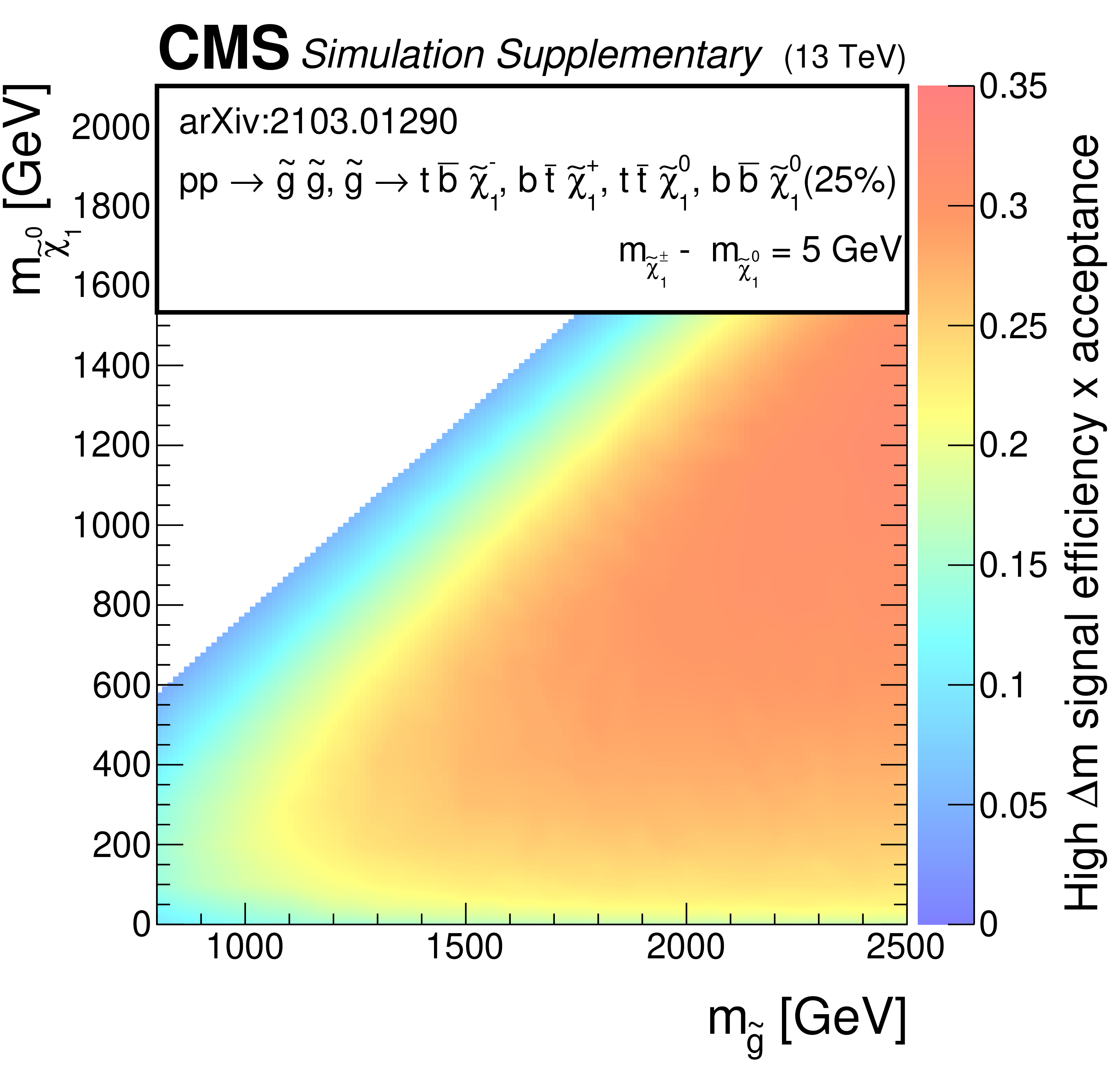
Additional Figure 18-a:
The efficiency times acceptance of the SMS gluino models for T1ttbb as a function of the gluino and LSP masses in the union of the 53 low ${\Delta m}$ search regions. |
png pdf |
Additional Figure 18-b:
The efficiency times acceptance of the SMS gluino models for T1ttbb as a function of the gluino and LSP masses in the union of the 130 high ${\Delta m}$ search regions. |

png pdf |
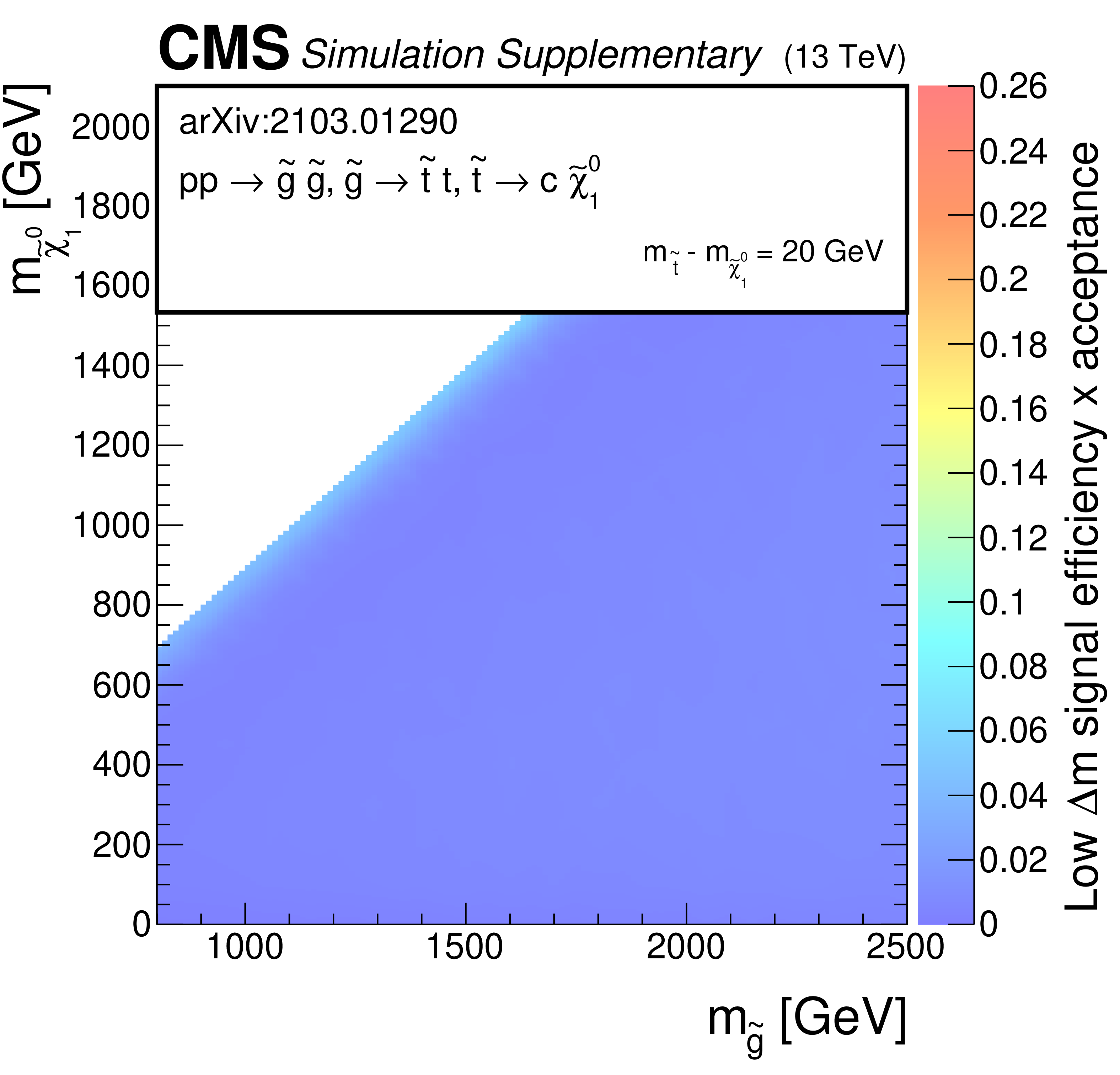
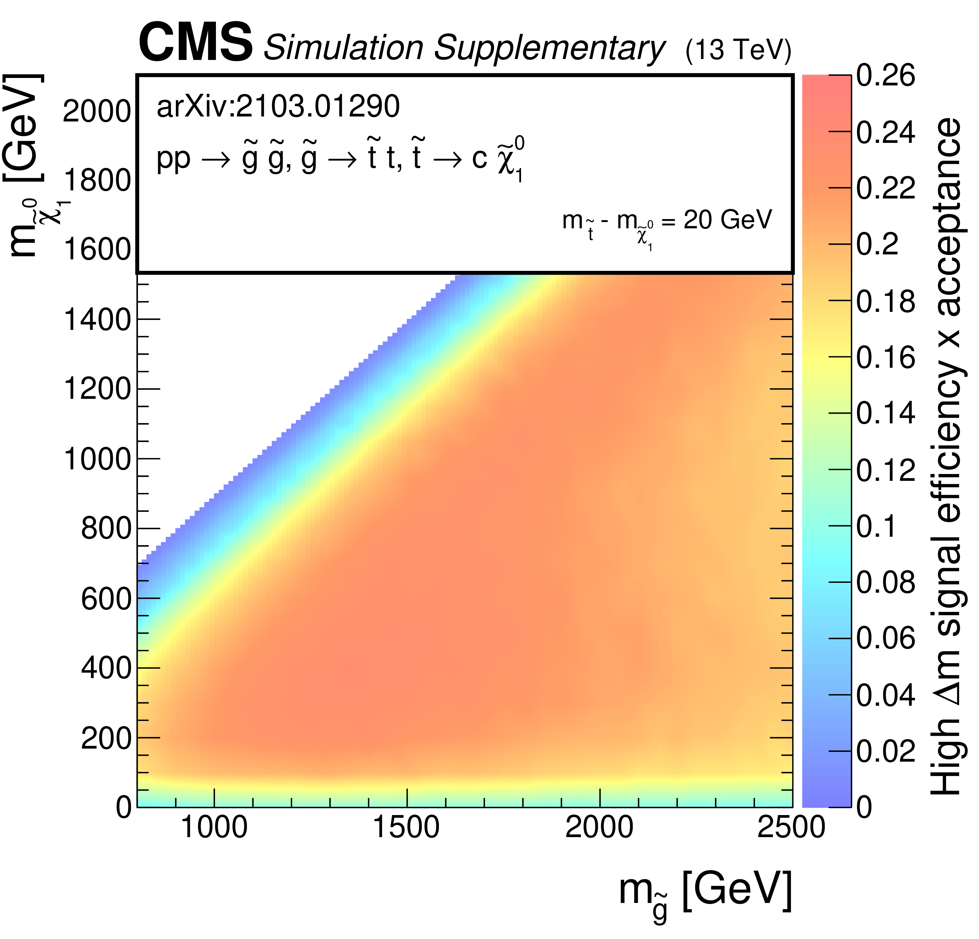
Additional Figure 19:
The efficiency times acceptance of the SMS gluino models for T5ttcc as a function of the gluino and LSP masses in the union of the 53 low ${\Delta m}$ search regions (left) and the 130 high ${\Delta m}$ search regions (right). |
png pdf |
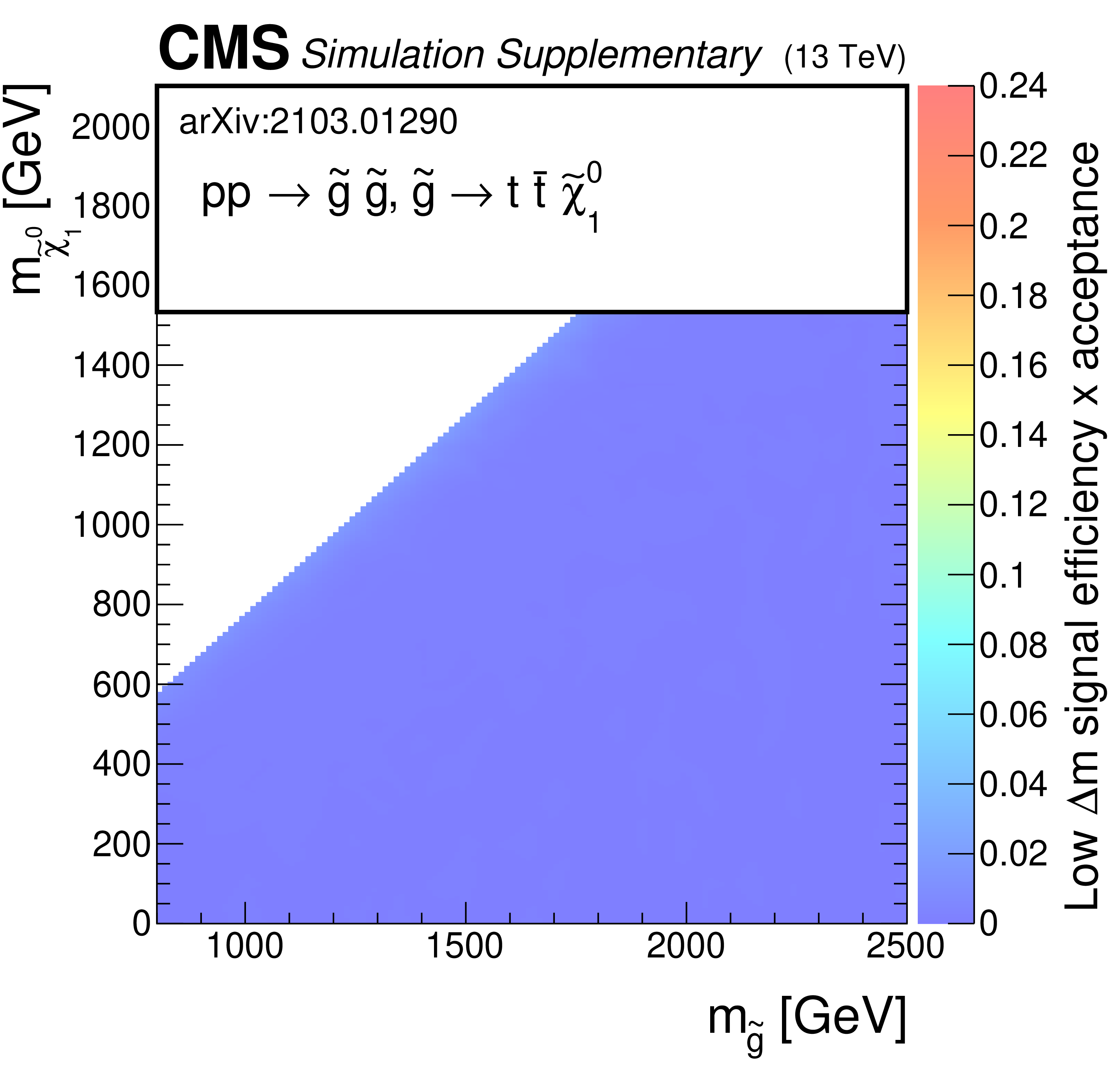
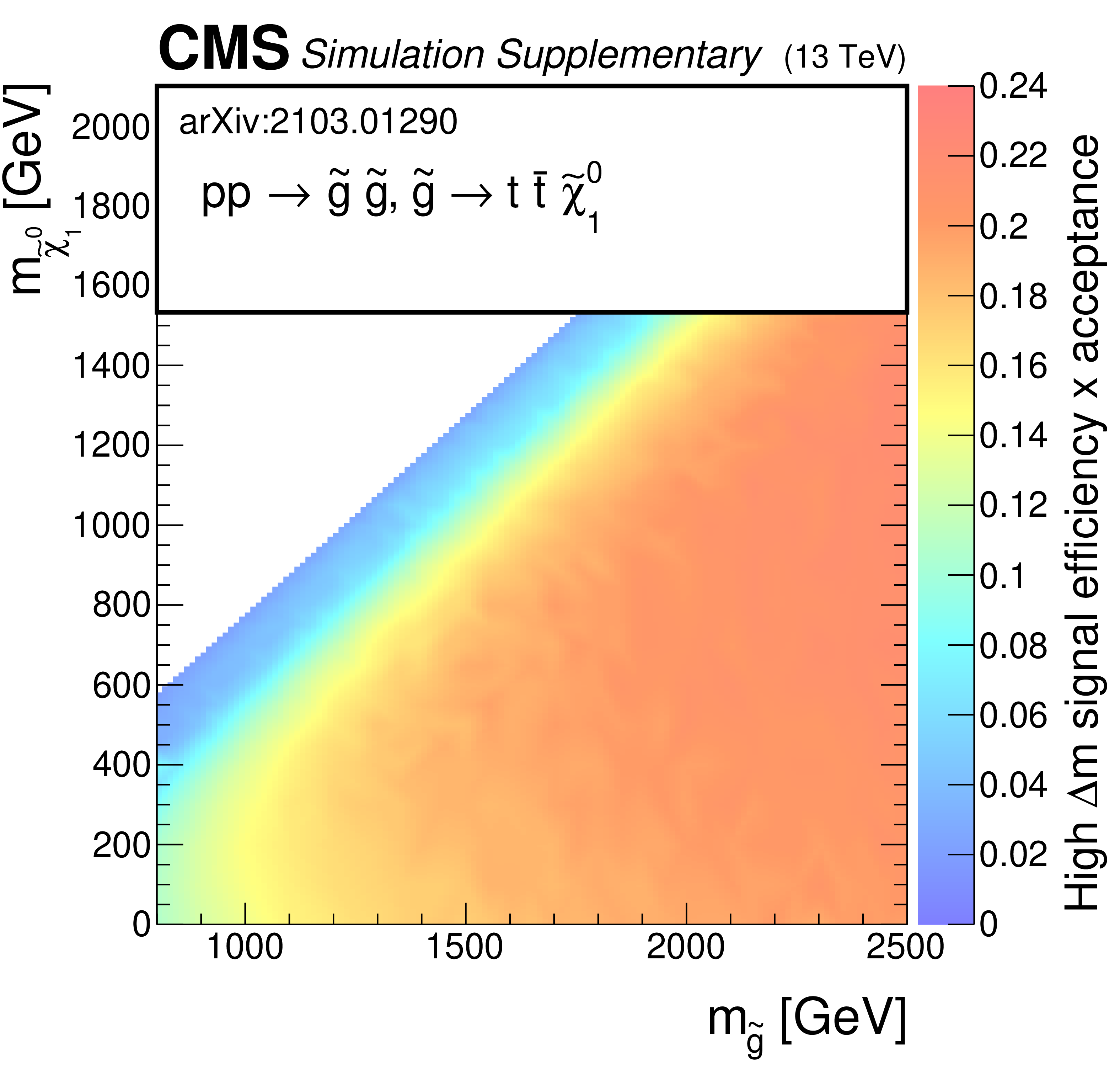
Additional Figure 19-a:
The efficiency times acceptance of the SMS gluino models for T5ttcc as a function of the gluino and LSP masses in the union of the 53 low ${\Delta m}$ search regions. |
png pdf |
Additional Figure 19-b:
The efficiency times acceptance of the SMS gluino models for T5ttcc as a function of the gluino and LSP masses in the union of the 130 high ${\Delta m}$ search regions. |
png pdf |
Additional Figure 20:
The expected and observed limits for T2ttC signal as a function of the top squark and LSP masses. |
png pdf |
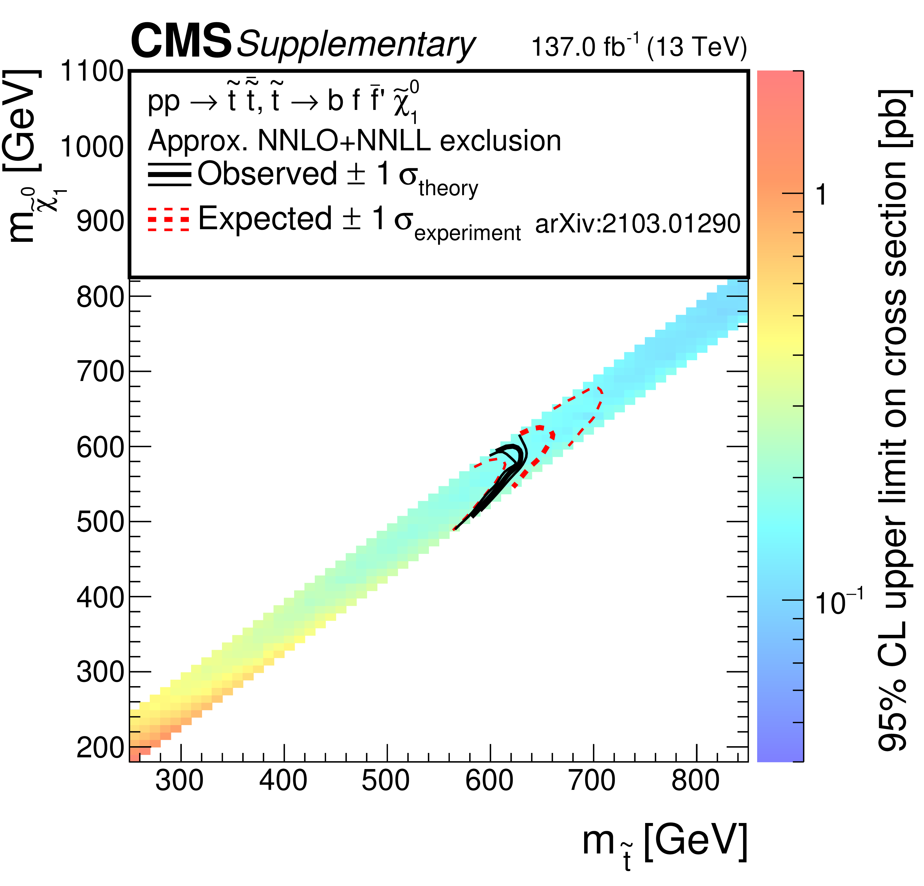
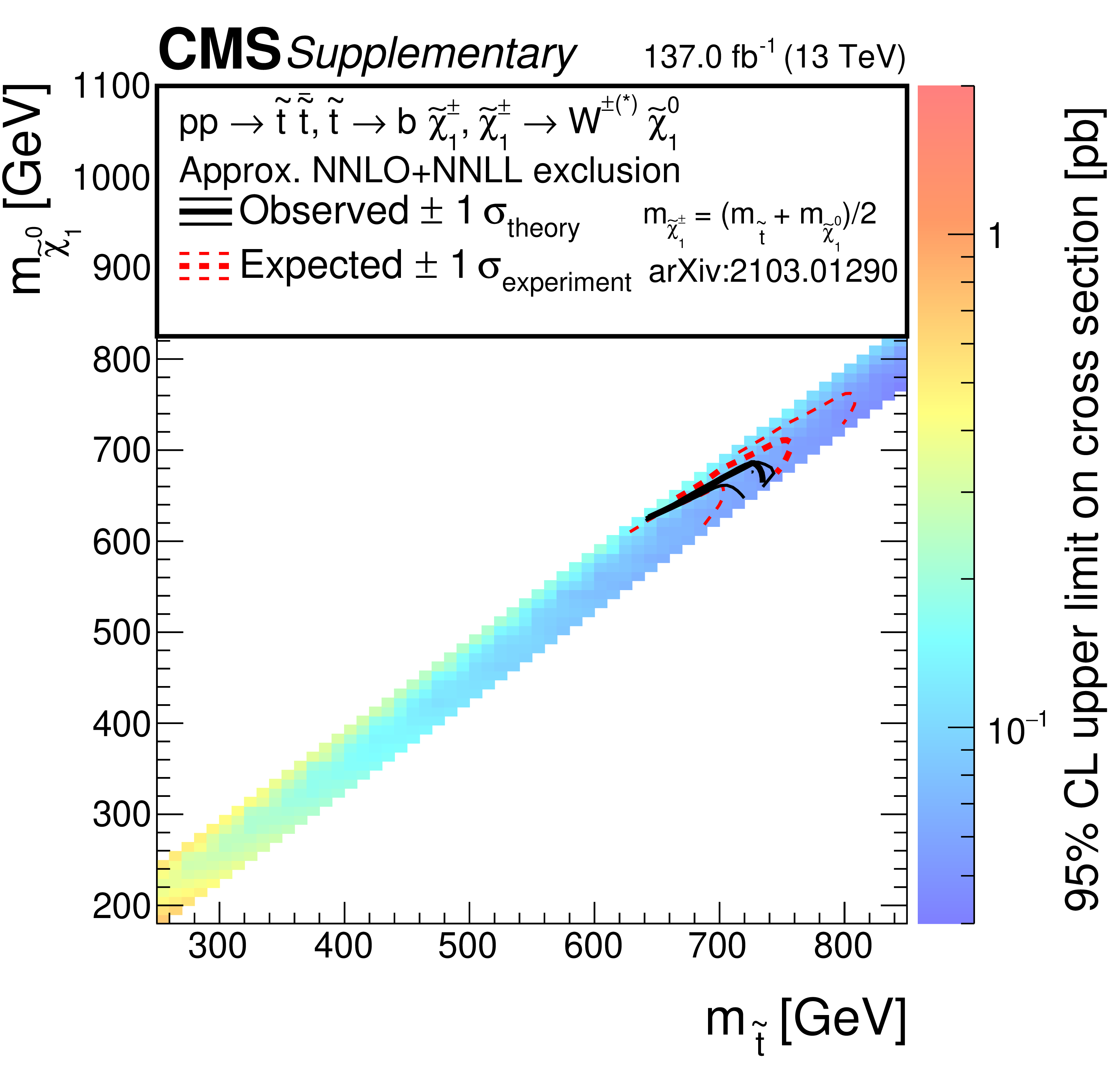
Additional Figure 21:
The expected and observed limits for T2bWC signal as a function of the top squark and LSP masses. |
png pdf |
Additional Figure 22:
The expected and observed limits for T2cc signal as a function of the top squark and LSP masses. |

png pdf |
Additional Figure 23:
The expected and observed limits for all of the signals for direct top squark production as a function of the top squark and LSP masses. |
| Additional Tables | |
png pdf |
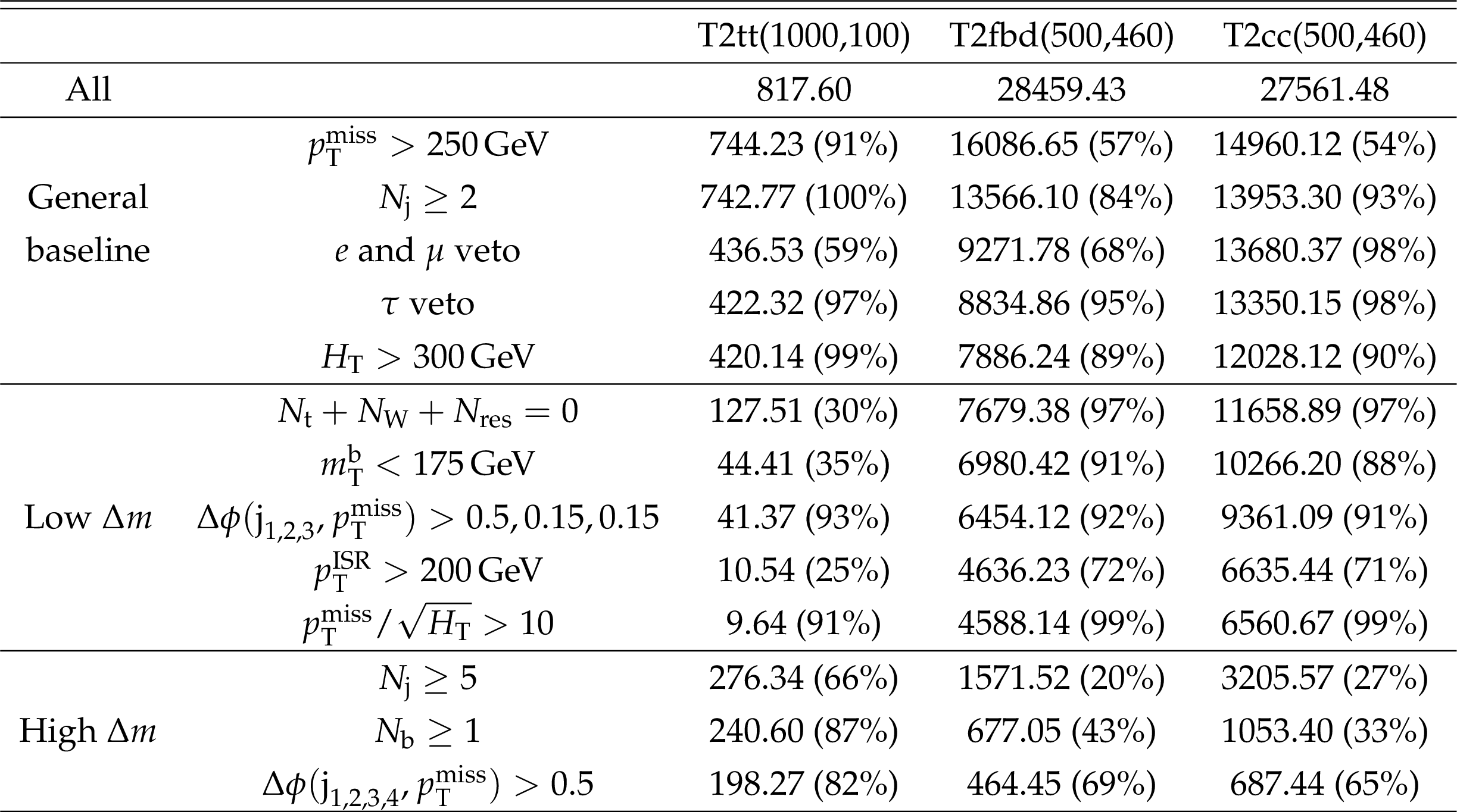
Additional Table 1:
The expected number of direct top squark production signal events that satisfy each selection requirement in turn. The percentages shown are the efficiency with respect to the previous line in most cases; the start of the low ${\Delta m}$ and high ${\Delta m}$ sections are with respect to the end of the general baseline. |

png pdf |
Additional Table 2:
The expected number of gluino-mediated top squark production signal events that satisfy each selection requirement in turn. All object and event weights are applied. Percentages shown are the efficiency with respect to the previous line in most cases; the start of the low ${\Delta m}$ and high ${\Delta m}$ sections are with respect to the end of the general baseline. |
png pdf |
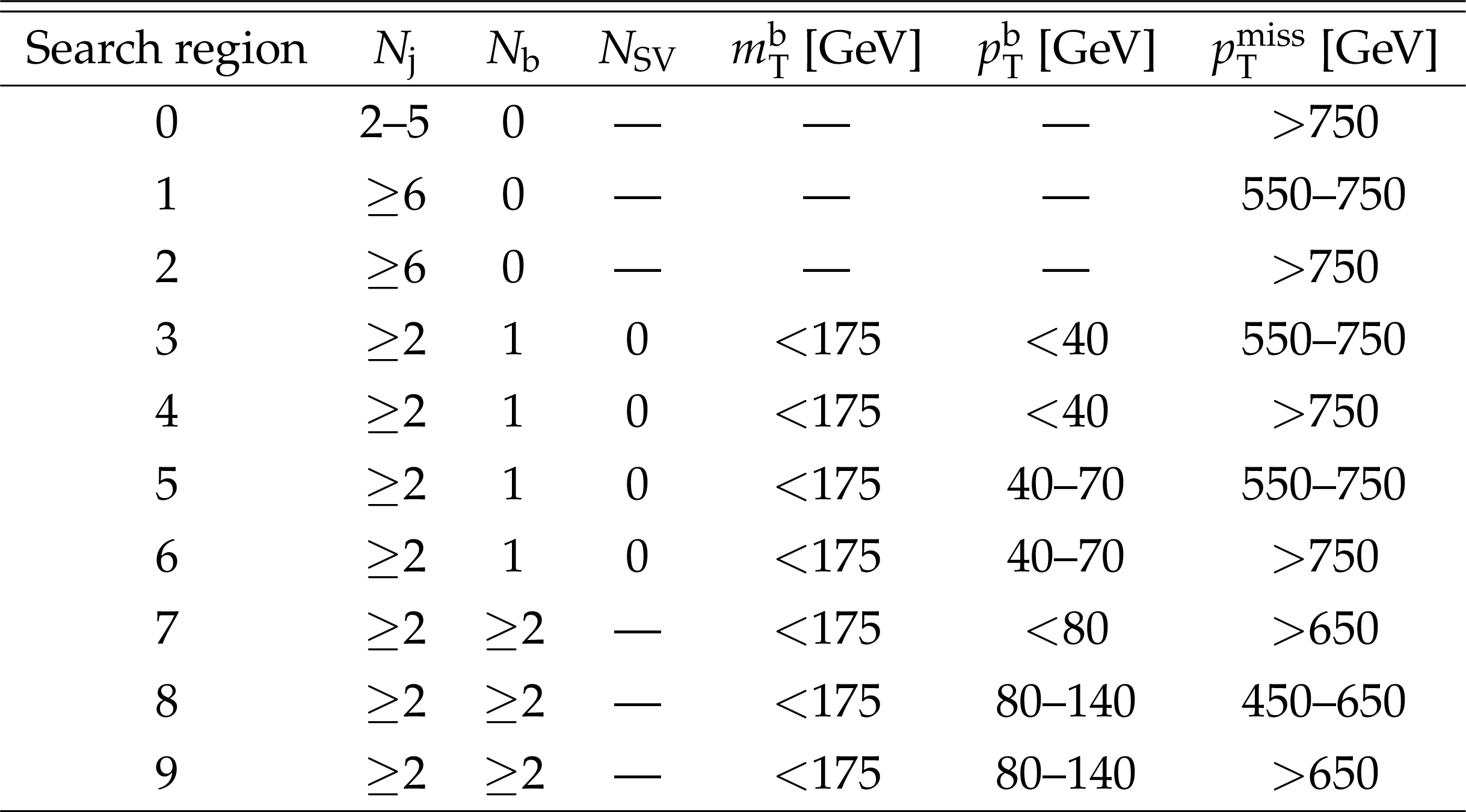
Additional Table 3:
Summary of the 10 disjoint super search regions in the low ${\Delta m}$ category. |

png pdf |
Additional Table 4:
Summary of the 15 disjoint super search regions in the high ${\Delta m}$ category. The selection requirements $ {{\Delta \phi} (\text {j}_{\text {1,2,3,4}}, {{p_{\mathrm {T}}} ^\text {miss}})} > 0.5$ and zero leptons are common to all high ${\Delta m}$ regions. A dash ({\text {--}}) indicates that no requirements are made. |
png pdf |
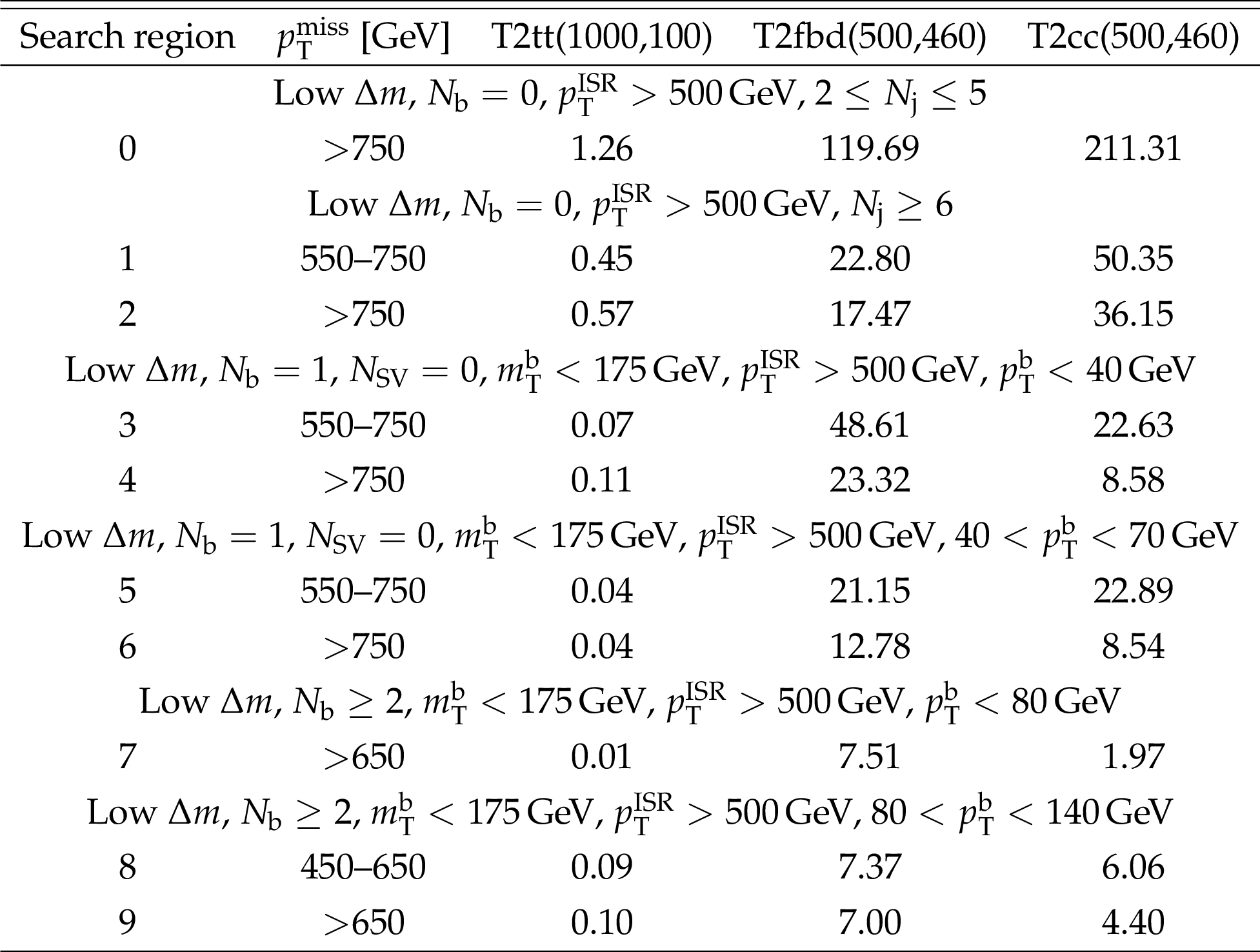
Additional Table 5:
Predicted event yields in super search regions 0-9 for a selection of direct top squark production signals. |
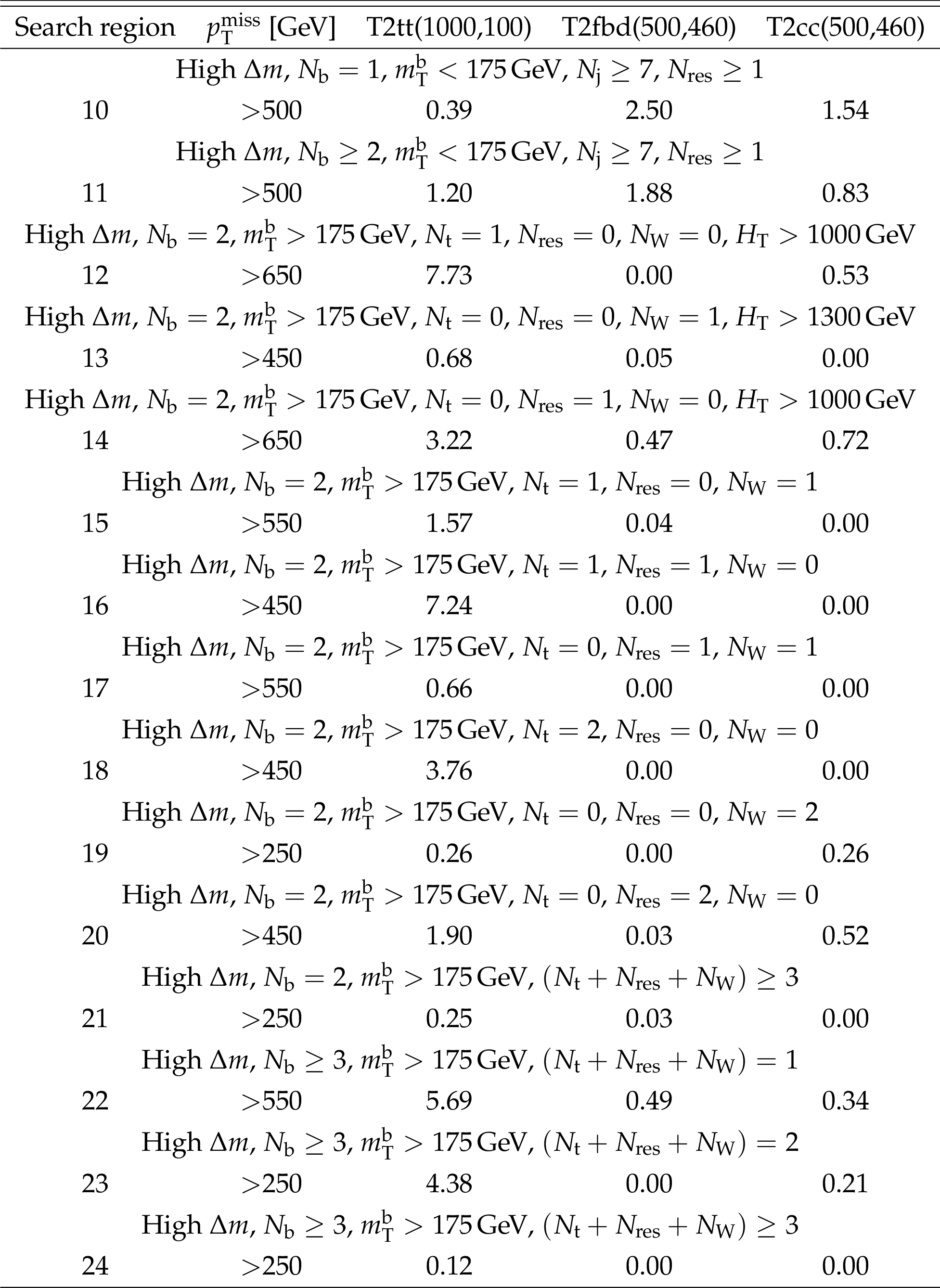
png pdf |
Additional Table 6:
Predicted event yields in super search regions 10-24 for a selection of direct top squark production signals. |

png pdf |
Additional Table 7:
Predicted event yields in super search regions 0-9 for a selection of gluino-mediated production signals. |

png pdf |
Additional Table 8:
Predicted event yields in super search regions 10-24 for a selection of gluino-mediated production signals. |
png pdf |
Additional Table 9:
Prediction for bins 0-9 |
png pdf |
Additional Table 10:
Prediction for bins 10-24 |
| References | ||||
| 1 | R. Barbieri and G. F. Giudice | Upper bounds on supersymmetric particle masses | NPB 306 (1988) 63 | |
| 2 | V. C. Rubin and W. K. Ford, Jr. | Rotation of the Andromeda nebula from a spectroscopic survey of emission regions | Astrophys. J. 159 (1970) 379 | |
| 3 | J. Wess and B. Zumino | A Lagrangian model invariant under supergauge transformations | PLB 49 (1974) 52 | |
| 4 | P. Fayet and S. Ferrara | Supersymmetry | PR 32 (1977) 249 | |
| 5 | R. Barbieri, S. Ferrara, and C. A. Savoy | Gauge models with spontaneously broken local supersymmetry | PLB 119 (1982) 343 | |
| 6 | H. P. Nilles | Supersymmetry, supergravity and particle physics | PR 110 (1984) 1 | |
| 7 | H. E. Haber and G. L. Kane | The search for supersymmetry: probing physics beyond the standard model | PR 117 (1985) 75 | |
| 8 | S. P. Martin | A supersymmetry primer | in Perspectives on supersymmetry. Vol.2, G. L. Kane, ed., volume 21, p. 1 2010 | hep-ph/9709356 |
| 9 | B. de Carlos and J. A. Casas | One-loop analysis of the electroweak breaking in supersymmetric models and the fine tuning problem | PLB 309 (1993) 320 | hep-ph/9303291 |
| 10 | S. Dimopoulos and G. F. Giudice | Naturalness constraints in supersymmetric theories with nonuniversal soft terms | PLB 357 (1995) 573 | hep-ph/9507282 |
| 11 | M. Papucci, J. T. Ruderman, and A. Weiler | Natural SUSY endures | JHEP 09 (2012) 035 | 1110.6926 |
| 12 | C. Brust, A. Katz, S. Lawrence, and R. Sundrum | SUSY, the third generation and the LHC | JHEP 03 (2012) 103 | 1110.6670 |
| 13 | A. Delgado et al. | The light stop window | EPJC 73 (2013) 2370 | 1212.6847 |
| 14 | C. Han et al. | Top-squark in natural SUSY under current LHC run-2 data | EPJC 77 (2017) 93 | 1609.02361 |
| 15 | H. Baer et al. | Gluino reach and mass extraction at the LHC in radiatively-driven natural SUSY | EPJC 77 (2017) 499 | 1612.00795 |
| 16 | H. Baer, V. Barger, N. Nagata, and M. Savoy | Phenomenological profile of top squarks from natural supersymmetry at the LHC | PRD 95 (2017) 055012 | 1611.08511 |
| 17 | J. L. Feng | Naturalness and the status of supersymmetry | Ann. Rev. Nucl. Part. Sci. 63 (2013) 351 | 1302.6587 |
| 18 | G. R. Farrar and P. Fayet | Phenomenology of the production, decay, and detection of new hadronic states associated with supersymmetry | PLB 76 (1978) 575 | |
| 19 | ATLAS Collaboration | Search for top squarks in final states with one isolated lepton, jets, and missing transverse momentum in $ \sqrt{s}= $ 13 TeV pp collisions with the ATLAS detector | PRD 94 (2016) 052009 | 1606.03903 |
| 20 | ATLAS Collaboration | Search for direct top squark pair production in events with a Higgs or $ Z $ boson, and missing transverse momentum in $ \sqrt{s}= $ 13 TeV pp collisions with the ATLAS detector | JHEP 08 (2017) 006 | 1706.03986 |
| 21 | ATLAS Collaboration | Search for direct top squark pair production in final states with two leptons in $ \sqrt{s} = $ 13 TeV pp collisions with the ATLAS detector | EPJC 77 (2017) 898 | 1708.03247 |
| 22 | ATLAS Collaboration | Search for a scalar partner of the top quark in the jets plus missing transverse momentum final state at $ \sqrt{s}= $ 13 TeV with the ATLAS detector | JHEP 12 (2017) 085 | 1709.04183 |
| 23 | ATLAS Collaboration | Search for $ B-L R $-parity-violating top squarks in $ \sqrt{s}= $ 13 TeV pp collisions with the ATLAS experiment | PRD 97 (2018) 032003 | 1710.05544 |
| 24 | ATLAS Collaboration | A search for pair-produced resonances in four-jet final states at $ \sqrt{s}= $ 13 TeV with the ATLAS detector | EPJC 78 (2018) 250 | 1710.07171 |
| 25 | ATLAS Collaboration | Search for top-squark pair production in final states with one lepton, jets, and missing transverse momentum using 36 fb$ {}^{-1} $ of $ \sqrt{s}= $ 13 TeV pp collision data with the ATLAS detector | JHEP 06 (2018) 108 | 1711.11520 |
| 26 | ATLAS Collaboration | Search for top squarks decaying to tau sleptons in pp collisions at $ \sqrt{s}= $ 13 TeV with the ATLAS detector | PRD 98 (2018) 032008 | 1803.10178 |
| 27 | ATLAS Collaboration | Search for supersymmetry in final states with charm jets and missing transverse momentum in 13 TeV pp collisions with the ATLAS detector | JHEP 09 (2018) 050 | 1805.01649 |
| 28 | ATLAS Collaboration | Search for heavy charged long-lived particles in proton-proton collisions at $ \sqrt{s} = $ 13 TeV using an ionisation measurement with the ATLAS detector | PLB 788 (2019) 96 | 1808.04095 |
| 29 | ATLAS Collaboration | Search for heavy charged long-lived particles in the ATLAS detector in 36.1 fb$ ^{-1} $ of proton-proton collision data at $ \sqrt{s} = $ 13 TeV | PRD 99 (2019) 092007 | 1902.01636 |
| 30 | ATLAS Collaboration | Search for a scalar partner of the top quark in the all-hadronic $ t{\bar{t}} $ plus missing transverse momentum final state at $ \sqrt{s} = $ 13 TeV with the ATLAS detector | EPJC 80 (2020) 737 | 2004.14060 |
| 31 | ATLAS Collaboration | Search for phenomena beyond the standard model in events with large $ b $-jet multiplicity using the ATLAS detector at the LHC | EPJC 81 (2021) 11 | 2010.01015 |
| 32 | ATLAS Collaboration | Search for top squarks in events with a Higgs or $ Z $ boson using 139 fb$ ^{-1} $ of $ pp $ collision data at $ \sqrt{s}= $ 13 TeV with the ATLAS detector | EPJC 80 (2020) 1080 | 2006.05880 |
| 33 | ATLAS Collaboration | Search for long-lived, massive particles in events with a displaced vertex and a muon with large impact parameter in $ pp $ collisions at $ \sqrt{s} = $ 13 TeV with the ATLAS detector | PRD 102 (2020) 032006 | 2003.11956 |
| 34 | ATLAS Collaboration | Search for squarks and gluinos in final states with same-sign leptons and jets using 139 fb$ ^{-1} $ of data collected with the ATLAS detector | JHEP 06 (2020) 046 | 1909.08457 |
| 35 | ATLAS Collaboration | Search for new phenomena with top quark pairs in final states with one lepton, jets, and missing transverse momentum in $ pp $ collisions at $ \sqrt{s} = $ 13 TeV with the ATLAS detector | Submitted to JHEP | 2012.03799 |
| 36 | ATLAS Collaboration | Search for new phenomena in events with two opposite-charge leptons, jets and missing transverse momentum in $ pp $ collisions at $ \sqrt{s} = $ 13 TeV with the ATLAS detector | Submitted to JHEP | 2102.01444 |
| 37 | CMS Collaboration | Searches for pair production of third-generation squarks in $ \sqrt{s}= $ 13 TeV pp collisions | EPJC 77 (2017) 327 | CMS-SUS-16-008 1612.03877 |
| 38 | CMS Collaboration | Search for supersymmetry in the all-hadronic final state using top quark tagging in pp collisions at $ \sqrt{s}= $ 13 TeV | PRD 96 (2017) 012004 | CMS-SUS-16-009 1701.01954 |
| 39 | CMS Collaboration | Search for top squark pair production in pp collisions at $ \sqrt{s}= $ 13 TeV using single lepton events | JHEP 10 (2017) 019 | CMS-SUS-16-051 1706.04402 |
| 40 | CMS Collaboration | Search for direct production of supersymmetric partners of the top quark in the all-jets final state in proton-proton collisions at $ \sqrt{s}= $ 13 TeV | JHEP 10 (2017) 005 | CMS-SUS-16-049 1707.03316 |
| 41 | CMS Collaboration | Search for supersymmetry in proton-proton collisions at 13 TeV using identified top quarks | PRD 97 (2018) 012007 | CMS-SUS-16-050 1710.11188 |
| 42 | CMS Collaboration | Search for the pair production of third-generation squarks with two-body decays to a bottom or charm quark and a neutralino in proton-proton collisions at $ \sqrt{s} = $ 13 TeV | PLB 778 (2018) 263 | CMS-SUS-16-032 1707.07274 |
| 43 | CMS Collaboration | Search for top squarks and dark matter particles in opposite-charge dilepton final states at $ \sqrt{s} = $ 13 TeV | PRD 97 (2018) 032009 | CMS-SUS-17-001 1711.00752 |
| 44 | CMS Collaboration | Search for new physics in events with two soft oppositely charged leptons and missing transverse momentum in proton-proton collisions at $ \sqrt{s} = $ 13 TeV | PLB 782 (2018) 440 | CMS-SUS-16-048 1801.01846 |
| 45 | CMS Collaboration | Search for pair-produced resonances decaying to quark pairs in proton-proton collisions at $ \sqrt{s} = $ 13 TeV | PRD 98 (2018) 112014 | CMS-EXO-17-021 1808.03124 |
| 46 | CMS Collaboration | Search for the pair production of light top squarks in the e$ ^{\pm}\mu^{\mp} $ final state in proton-proton collisions at $ \sqrt{s} = $ 13 TeV | JHEP 03 (2019) 101 | CMS-SUS-18-003 1901.01288 |
| 47 | CMS Collaboration | Search for direct top squark pair production in events with one lepton, jets, and missing transverse momentum at 13 TeV with the CMS experiment | JHEP 05 (2020) 032 | CMS-SUS-19-009 1912.08887 |
| 48 | CMS Collaboration | Search for top squark pair production using dilepton final states in pp collision data collected at $ \sqrt{s}= $ 13 TeV | EPJC 81 (2021) 3 | CMS-SUS-19-011 2008.05936 |
| 49 | CMS Collaboration | Identification of heavy-flavour jets with the CMS detector in pp collisions at 13 TeV | JINST 13 (2018) P05011 | CMS-BTV-16-002 1712.07158 |
| 50 | CMS Collaboration | Identification of heavy, energetic, hadronically decaying particles using machine-learning techniques | JINST 15 (2020) P06005 | CMS-JME-18-002 2004.08262 |
| 51 | J. Alwall, M.-P. Le, M. Lisanti, and J. G. Wacker | Model-independent jets plus missing energy searches | PRD 79 (2009) 015005 | 0809.3264 |
| 52 | J. Alwall, P. C. Schuster, and N. Toro | Simplified models for a first characterization of new physics at the LHC | PRD 79 (2009) 075020 | 0810.3921 |
| 53 | D. Alves et al. | Simplified models for LHC new physics searches | JPG 39 (2012) 105005 | 1105.2838 |
| 54 | CMS Collaboration | Interpretation of searches for supersymmetry with simplified models | PRD 88 (2013) 052017 | CMS-SUS-11-016 1301.2175 |
| 55 | C. Balazs, M. Carena, and C. E. M. Wagner | Dark matter, light top squarks and electroweak baryogenesis | PRD 70 (2004) 015007 | hep-ph/0403224 |
| 56 | J. Ellis, K. A. Olive, and Y. Santoso | Calculations of neutralino-stop coannihilation in the CMSSM | Astropart. Phys. 18 (2003) 395 | hep-ph/0112113 |
| 57 | J. Ellis, K. A. Olive, and J. Zheng | The extent of the stop coannihilation strip | EPJC 74 (2014) 2947 | 1404.5571 |
| 58 | CMS Collaboration | The CMS trigger system | JINST 12 (2017) P01020 | CMS-TRG-12-001 1609.02366 |
| 59 | CMS Collaboration | CMS luminosity measurements for the 2016 data taking period | CMS-PAS-LUM-17-001 | CMS-PAS-LUM-17-001 |
| 60 | CMS Collaboration | CMS luminosity measurement for the 2017 data-taking period at $ \sqrt{s} = $ 13 TeV | CMS-PAS-LUM-17-004 | CMS-PAS-LUM-17-004 |
| 61 | CMS Collaboration | CMS luminosity measurement for the 2018 data-taking period at $ \sqrt{s} = $ 13 TeV | CMS-PAS-LUM-18-002 | CMS-PAS-LUM-18-002 |
| 62 | CMS Collaboration | The CMS experiment at the CERN LHC | JINST 3 (2008) S08004 | CMS-00-001 |
| 63 | J. Alwall et al. | The automated computation of tree-level and next-to-leading order differential cross sections, and their matching to parton shower simulations | JHEP 07 (2014) 079 | 1405.0301 |
| 64 | W. Beenakker et al. | NNLL-fast: predictions for coloured supersymmetric particle production at the LHC with threshold and Coulomb resummation | JHEP 12 (2016) 133 | 1607.07741 |
| 65 | W. Beenakker, R. Hopker, M. Spira, and P. M. Zerwas | Squark and gluino production at hadron colliders | NPB 492 (1997) 51 | hep-ph/9610490 |
| 66 | A. Kulesza and L. Motyka | Threshold resummation for squark-antisquark and gluino-pair production at the LHC | PRL 102 (2009) 111802 | 0807.2405 |
| 67 | A. Kulesza and L. Motyka | Soft gluon resummation for the production of gluino-gluino and squark-antisquark pairs at the LHC | PRD 80 (2009) 095004 | 0905.4749 |
| 68 | W. Beenakker et al. | Soft-gluon resummation for squark and gluino hadroproduction | JHEP 12 (2009) 041 | 0909.4418 |
| 69 | W. Beenakker et al. | NNLL resummation for squark-antisquark pair production at the LHC | JHEP 01 (2012) 076 | 1110.2446 |
| 70 | W. Beenakker et al. | Towards NNLL resummation: hard matching coefficients for squark and gluino hadroproduction | JHEP 10 (2013) 120 | 1304.6354 |
| 71 | W. Beenakker et al. | NNLL resummation for squark and gluino production at the LHC | JHEP 12 (2014) 023 | 1404.3134 |
| 72 | W. Beenakker et al. | Stop production at hadron colliders | NPB 515 (1998) 3 | hep-ph/9710451 |
| 73 | W. Beenakker et al. | Supersymmetric top and bottom squark production at hadron colliders | JHEP 08 (2010) 098 | 1006.4771 |
| 74 | W. Beenakker et al. | NNLL resummation for stop pair-production at the LHC | JHEP 05 (2016) 153 | 1601.02954 |
| 75 | R. Frederix and S. Frixione | Merging meets matching in MC@NLO | JHEP 12 (2012) 061 | 1209.6215 |
| 76 | P. Nason | A new method for combining NLO QCD with shower Monte Carlo algorithms | JHEP 11 (2004) 040 | hep-ph/0409146 |
| 77 | S. Frixione, P. Nason, and C. Oleari | Matching NLO QCD computations with parton shower simulations: the POWHEG method | JHEP 11 (2007) 070 | 0709.2092 |
| 78 | S. Alioli, P. Nason, C. Oleari, and E. Re | A general framework for implementing NLO calculations in shower Monte Carlo programs: the POWHEG BOX | JHEP 06 (2010) 043 | 1002.2581 |
| 79 | S. Alioli, P. Nason, C. Oleari, and E. Re | NLO single-top production matched with shower in POWHEG: $ s $- and $ t $-channel contributions | JHEP 09 (2009) 111 | 0907.4076 |
| 80 | E. Re | Single-top $ \text{Wt} $-channel production matched with parton showers using the POWHEG method | EPJC 71 (2011) 1547 | 1009.2450 |
| 81 | T. Melia, P. Nason, R. Rontsch, and G. Zanderighi | $ W^+W^- $, $ WZ $ and $ ZZ $ production in the POWHEG BOX | JHEP 11 (2011) 078 | 1107.5051 |
| 82 | P. Nason and G. Zanderighi | $ W^+W^- $, $ WZ $ and $ ZZ $ production in the POWHEG-BOX-V2 | EPJC 74 (2014) 2702 | 1311.1365 |
| 83 | H. B. Hartanto, B. Jager, L. Reina, and D. Wackeroth | Higgs boson production in association with top quarks in the POWHEG BOX | PRD 91 (2015) 094003 | 1501.04498 |
| 84 | T. Sjostrand et al. | An introduction to PYTHIA 8.2 | CPC 191 (2015) 159 | 1410.3012 |
| 85 | S. Quackenbush, R. Gavin, Y. Li, and F. Petriello | W physics at the LHC with FEWZ 2.1 | CPC 184 (2013) 209 | 1201.5896 |
| 86 | R. Gavin, Y. Li, F. Petriello, and S. Quackenbush | FEWZ 2.0: a code for hadronic Z production at next-to-next-to-leading order | CPC 182 (2011) 2388 | 1011.3540 |
| 87 | Y. Li and F. Petriello | Combining QCD and electroweak corrections to dilepton production in the framework of the FEWZ simulation code | PRD 86 (2012) 094034 | 1208.5967 |
| 88 | T. Gehrmann et al. | $ W^+W^- $ production at hadron colliders in next to next to leading order QCD | PRL 113 (2014) 212001 | 1408.5243 |
| 89 | J. M. Campbell, R. K. Ellis, and C. Williams | Vector boson pair production at the LHC | JHEP 07 (2011) 018 | 1105.0020 |
| 90 | M. Beneke, P. Falgari, S. Klein, and C. Schwinn | Hadronic top-quark pair production with NNLL threshold resummation | NPB 855 (2012) 695 | 1109.1536 |
| 91 | M. Cacciari et al. | Top-pair production at hadron colliders with next-to-next-to-leading logarithmic soft-gluon resummation | PLB 710 (2012) 612 | 1111.5869 |
| 92 | P. Barnreuther, M. Czakon, and A. Mitov | Percent-level-precision physics at the Tevatron: next-to-next-to-leading order QCD corrections to $ \mathrm{q\bar{q}} \to \mathrm{t\bar{t}} + {X} $ | PRL 109 (2012) 132001 | 1204.5201 |
| 93 | M. Czakon and A. Mitov | NNLO corrections to top-pair production at hadron colliders: the all-fermionic scattering channels | JHEP 12 (2012) 054 | 1207.0236 |
| 94 | M. Czakon and A. Mitov | NNLO corrections to top pair production at hadron colliders: the quark-gluon reaction | JHEP 01 (2013) 080 | 1210.6832 |
| 95 | M. Czakon, P. Fiedler, and A. Mitov | Total top-quark pair-production cross section at hadron colliders through $ O({\alpha_S}^4) $ | PRL 110 (2013) 252004 | 1303.6254 |
| 96 | M. Czakon and A. Mitov | Top++: a program for the calculation of the top-pair cross-section at hadron colliders | CPC 185 (2014) 2930 | 1112.5675 |
| 97 | M. L. Mangano, M. Moretti, F. Piccinini, and M. Treccani | Matching matrix elements and shower evolution for top-pair production in hadronic collisions | JHEP 01 (2007) 013 | hep-ph/0611129 |
| 98 | CMS Collaboration | Event generator tunes obtained from underlying event and multiparton scattering measurements | EPJC 76 (2016) 155 | CMS-GEN-14-001 1512.00815 |
| 99 | CMS Collaboration | Extraction and validation of a new set of CMS PYTHIA8 tunes from underlying-event measurements | EPJC 80 (2020) 4 | CMS-GEN-17-001 1903.12179 |
| 100 | NNPDF Collaboration | Parton distributions with QED corrections | NPB 877 (2013) 290 | 1308.0598 |
| 101 | NNPDF Collaboration | Parton distributions from high-precision collider data | EPJC 77 (2017) 663 | 1706.00428 |
| 102 | GEANT4 Collaboration | GEANT4--a simulation toolkit | NIMA 506 (2003) 250 | |
| 103 | S. Abdullin et al. | The fast simulation of the CMS detector at LHC | J. Phys. Conf. Ser. 331 (2011) 032049 | |
| 104 | A. Giammanco | The fast simulation of the CMS experiment | J. Phys. Conf. Ser. 513 (2014) 022012 | |
| 105 | CMS Collaboration | Measurement of differential cross sections for top quark pair production using the lepton+jets final state in proton-proton collisions at 13 TeV | PRD 95 (2017) 092001 | CMS-TOP-16-008 1610.04191 |
| 106 | CMS Collaboration | Particle-flow reconstruction and global event description with the CMS detector | JINST 12 (2017) P10003 | CMS-PRF-14-001 1706.04965 |
| 107 | CMS Collaboration | Performance of missing transverse momentum reconstruction in proton-proton collisions at $ \sqrt{s} = $ 13 TeV using the CMS detector | JINST 14 (2019) P07004 | CMS-JME-17-001 1903.06078 |
| 108 | M. Cacciari, G. P. Salam, and G. Soyez | The anti-$ {k_{\mathrm{T}}} $ jet clustering algorithm | JHEP 04 (2008) 063 | 0802.1189 |
| 109 | M. Cacciari, G. P. Salam, and G. Soyez | FastJet user manual | EPJC 72 (2012) 1896 | 1111.6097 |
| 110 | CMS Collaboration | Pileup mitigation at CMS in 13 TeV data | JINST 15 (2020) P09018 | CMS-JME-18-001 2003.00503 |
| 111 | M. Cacciari and G. P. Salam | Pileup subtraction using jet areas | PLB 659 (2008) 119 | 0707.1378 |
| 112 | CMS Collaboration | Jet energy scale and resolution in the CMS experiment in pp collisions at 8 TeV | JINST 12 (2017) P02014 | CMS-JME-13-004 1607.03663 |
| 113 | CMS Collaboration | Measurement of $ B\overline{B} $ angular correlations based on secondary vertex reconstruction at $ \sqrt{s}= $ 7 TeV | JHEP 03 (2011) 136 | CMS-BPH-10-010 1102.3194 |
| 114 | D. Bertolini, P. Harris, M. Low, and N. Tran | Pileup per particle identification | JHEP 10 (2014) 059 | 1407.6013 |
| 115 | CMS Collaboration | Performance of electron reconstruction and selection with the CMS detector in proton-proton collisions at $ \sqrt{s}= $ 8 TeV | JINST 10 (2015) P06005 | CMS-EGM-13-001 1502.02701 |
| 116 | CMS Collaboration | Performance of the CMS muon detector and muon reconstruction with proton-proton collisions at $ \sqrt{s}= $ 13 TeV | JINST 13 (2018) P06015 | CMS-MUO-16-001 1804.04528 |
| 117 | CMS Collaboration | Reconstruction and identification of $ \tau $ lepton decays to hadrons and $ \nu_{\tau} $ at CMS | JINST 11 (2016) P01019 | CMS-TAU-14-001 1510.07488 |
| 118 | CMS Collaboration | Performance of reconstruction and identification of $ \tau $ leptons in their decays to hadrons and $ \nu_{\tau} $ in LHC Run-2 | CMS-PAS-TAU-16-002 | CMS-PAS-TAU-16-002 |
| 119 | CMS Collaboration | Performance of photon reconstruction and identification with the CMS detector in proton-proton collisions at $ \sqrt{s}= $ 8 TeV | JINST 10 (2015) P08010 | CMS-EGM-14-001 1502.02702 |
| 120 | CMS Collaboration | Performance of quark/gluon discrimination in 8 TeV pp data | CMS-PAS-JME-13-002 | CMS-PAS-JME-13-002 |
| 121 | Y. Ganin et al. | Domain-adversarial training of neural networks | in Domain Adaptation in Computer Vision Applications, G. Csurka, ed., Advances in Computer Vision and Pattern Recognition, Springer, Cham, Switzerland | 1505.07818 |
| 122 | CMS Collaboration | A deep neural network to search for new long-lived particles decaying to jets | Mach. Learn. Sci. Tech. 1 (2020) 035012 | CMS-EXO-19-011 1912.12238 |
| 123 | CMS Collaboration | Measurement of top quark pair production in association with a Z boson in proton-proton collisions at $ \sqrt{s} = $ 13 TeV | JHEP 03 (2020) 056 | CMS-TOP-18-009 1907.11270 |
| 124 | A. L. Read | Presentation of search results: The $ \mathrm{CL_s} $ technique | JPG 28 (2002) 2693 | |
| 125 | T. Junk | Confidence level computation for combining searches with small statistics | NIMA 434 (1999) 435 | hep-ex/9902006 |
| 126 | G. Cowan, K. Cranmer, E. Gross, and O. Vitells | Asymptotic formulae for likelihood-based tests of new physics | EPJC 71 (2011) 1554 | 1007.1727 |
| 127 | R. J. Barlow and C. Beeston | Fitting using finite Monte Carlo samples | CPC 77 (1993) 219 | |
| 128 | ATLAS Collaboration | Measurements of top-quark pair spin correlations in the $ e\mu $ channel at $ \sqrt{s} = $ 13 TeV using $ pp $ collisions in the ATLAS detector | EPJC 80 (2020) 754 | 1903.07570 |
| 129 | ALEPH Collaboration | Search for scalar quarks in $ e^{+} e^{-} $ collisions at $ \sqrt{s} $ up to 209 GeV | PLB 537 (2002) 5 | hep-ex/0204036 |
| 130 | DELPHI Collaboration | Searches for supersymmetric particles in $ e^{+} e^{-} $ collisions up to 208 GeV and interpretation of the results within the MSSM | EPJC 31 (2003) 421 | hep-ex/0311019 |
| 131 | L3 Collaboration | Search for scalar leptons and scalar quarks at LEP | PLB 580 (2004) 37 | hep-ex/0310007 |
| 132 | OPAL Collaboration | Search for scalar top and scalar bottom quarks at LEP | PLB 545 (2002) 272 | hep-ex/0209026 |
|
|
Compact Muon Solenoid LHC, CERN |
|

|

|

|

|

|