

Compact Muon Solenoid
LHC, CERN
| CMS-TOP-21-004 ; CERN-EP-2021-192 | ||
| Measurement of the inclusive and differential ${\mathrm{t\bar{t}}\gamma}$ cross sections in the dilepton channel and effective field theory interpretation in proton-proton collisions at $\sqrt{s} = $ 13 TeV | ||
| CMS Collaboration | ||
| 18 January 2022 | ||
| JHEP 05 (2022) 091 | ||
| Abstract: The production cross section of a top quark pair in association with a photon is measured in proton-proton collisions in the decay channel with two oppositely charged leptons (${\mathrm{e^{\pm}}\mu^{\mp}} $, ${\mathrm{e^{+}}\mathrm{e^{-}}} $, or $\mu^{+}\mu^{-}$). The measurement is performed using 138 fb$^{-1}$ of proton-proton collision data recorded by the CMS experiment at $\sqrt{s} =$ 13 TeV during the 2016-2018 data-taking period of the CERN LHC. A fiducial phase space is defined such that photons radiated by initial-state particles, top quarks, or any of their decay products are included. An inclusive cross section of 173.5 $\pm$ 2.5 (stat) $\pm$ 6.3 (syst) fb is measured in a signal region with at least one jet coming from the hadronization of a bottom quark and exactly one photon with transverse momentum above 20 GeV. Differential cross sections are measured as functions of several kinematic observables of the photon, leptons, and jets, and compared to standard model predictions. The measurements are also interpreted in the standard model effective field theory framework, and limits are found on the relevant Wilson coefficients from these results alone and in combination with a previous CMS measurement of the ${\mathrm{t\bar{t}}\gamma}$ production process using the lepton+jets final state. | ||
| Links: e-print arXiv:2201.07301 [hep-ex] (PDF) ; CDS record ; inSPIRE record ; HepData record ; CADI line (restricted) ; | ||
| Figures & Tables | Summary | Additional Figures | References | CMS Publications |
|---|
| Figures | |

png pdf |
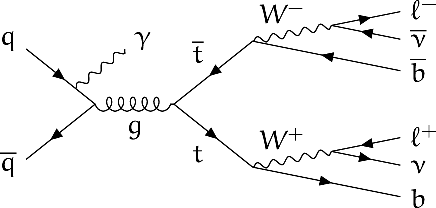
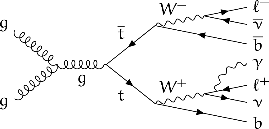
Figure 1:
Examples of leading-order Feynman diagrams for ${{\mathrm{t} \mathrm{\bar{t}}} \gamma}$ production with two leptons in the final state, where the photon is radiated by a top quark (left), by an incoming quark (middle), or by one of the charged decay products of a top quark (right). |

png pdf |
Figure 1-a:
Example of leading-order Feynman diagram for ${{\mathrm{t} \mathrm{\bar{t}}} \gamma}$ production with two leptons in the final state, where the photon is radiated by a top quark. |
png pdf |
Figure 1-b:
Example of leading-order Feynman diagram for ${{\mathrm{t} \mathrm{\bar{t}}} \gamma}$ production with two leptons in the final state, where the photon is radiated by an incoming quark. |
png pdf |
Figure 1-c:
Example of leading-order Feynman diagram for ${{\mathrm{t} \mathrm{\bar{t}}} \gamma}$ production with two leptons in the final state, where the photon is radiated by one of the charged decay products of a top quark. |

png pdf |
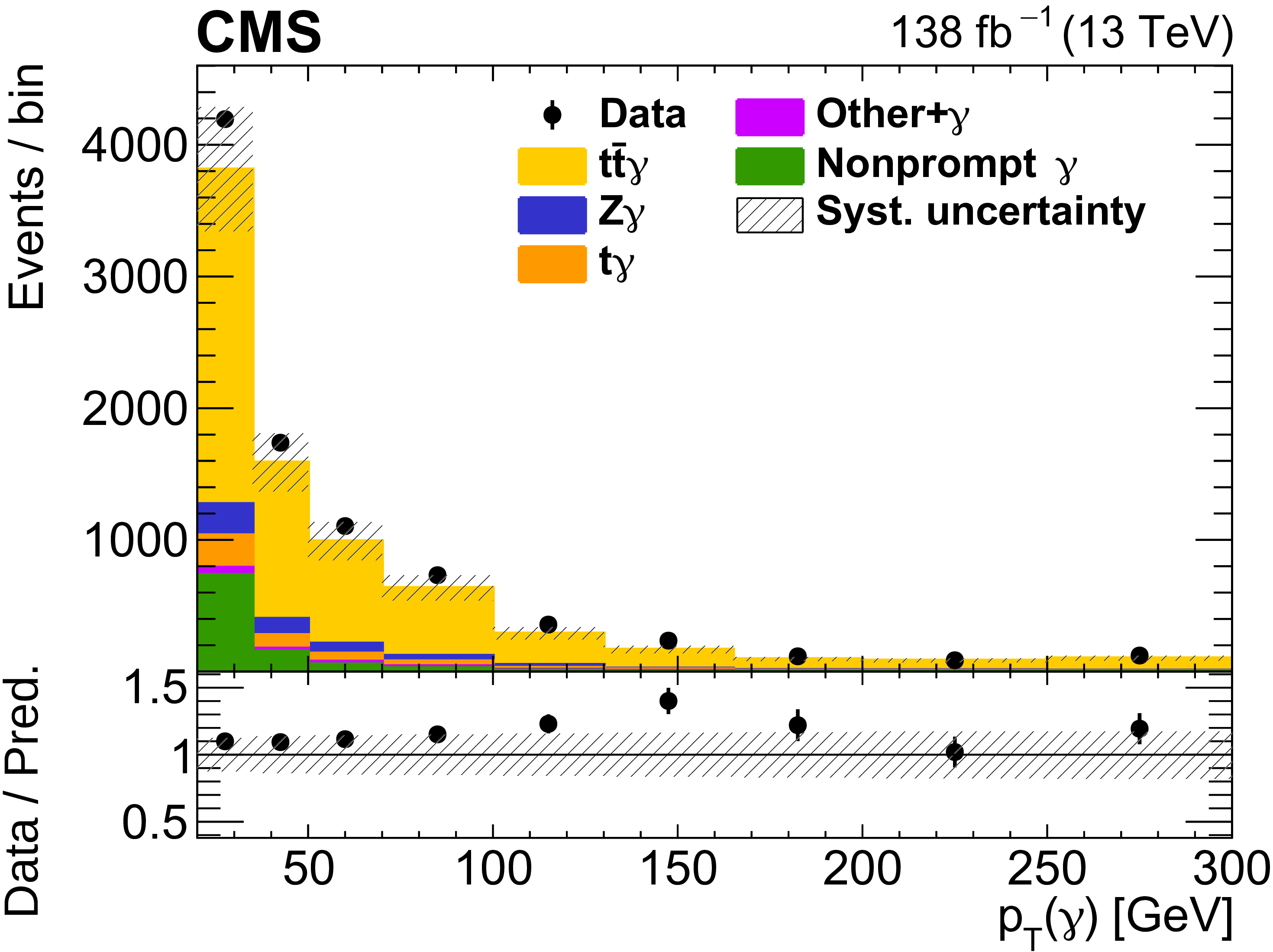
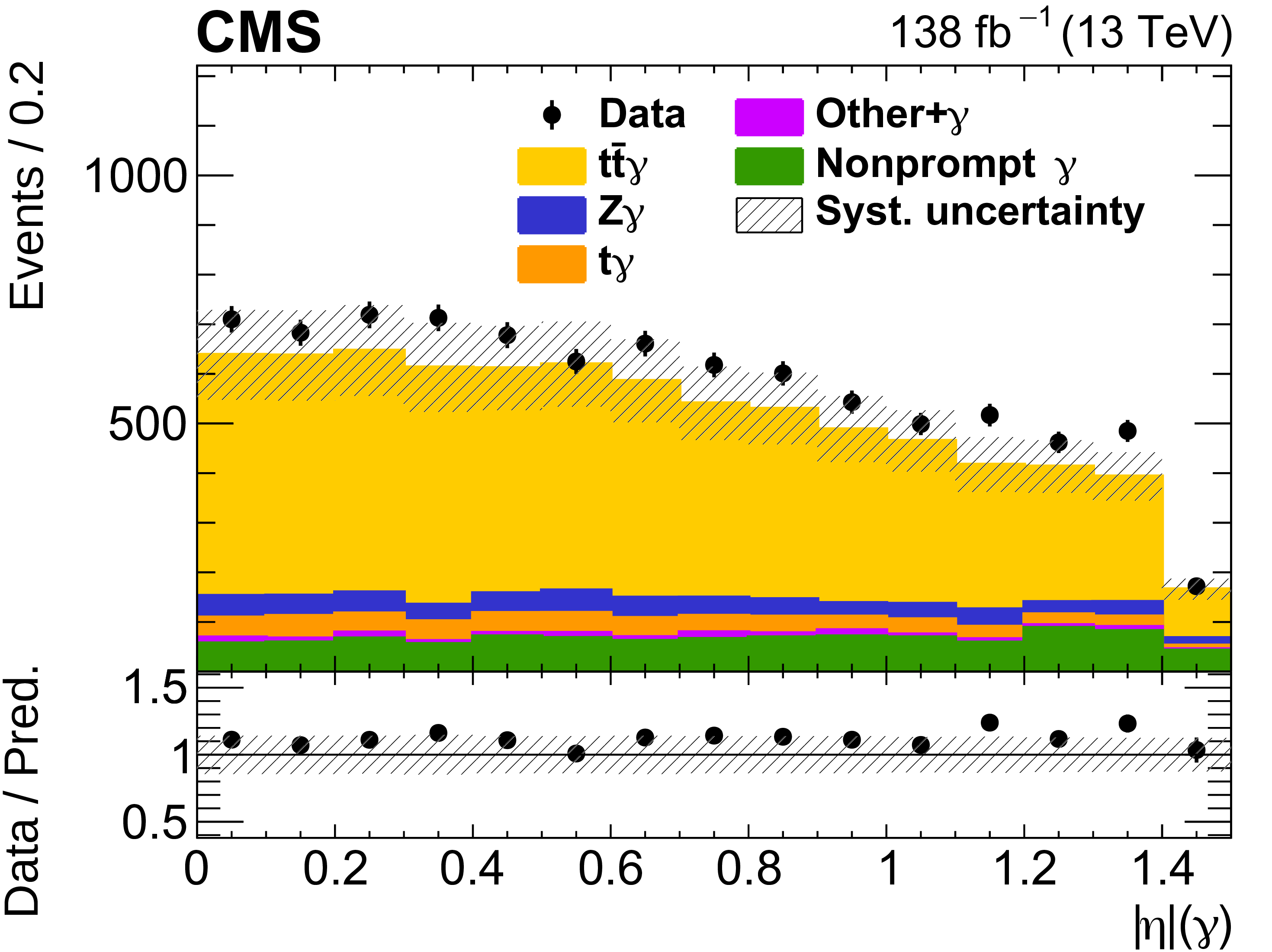
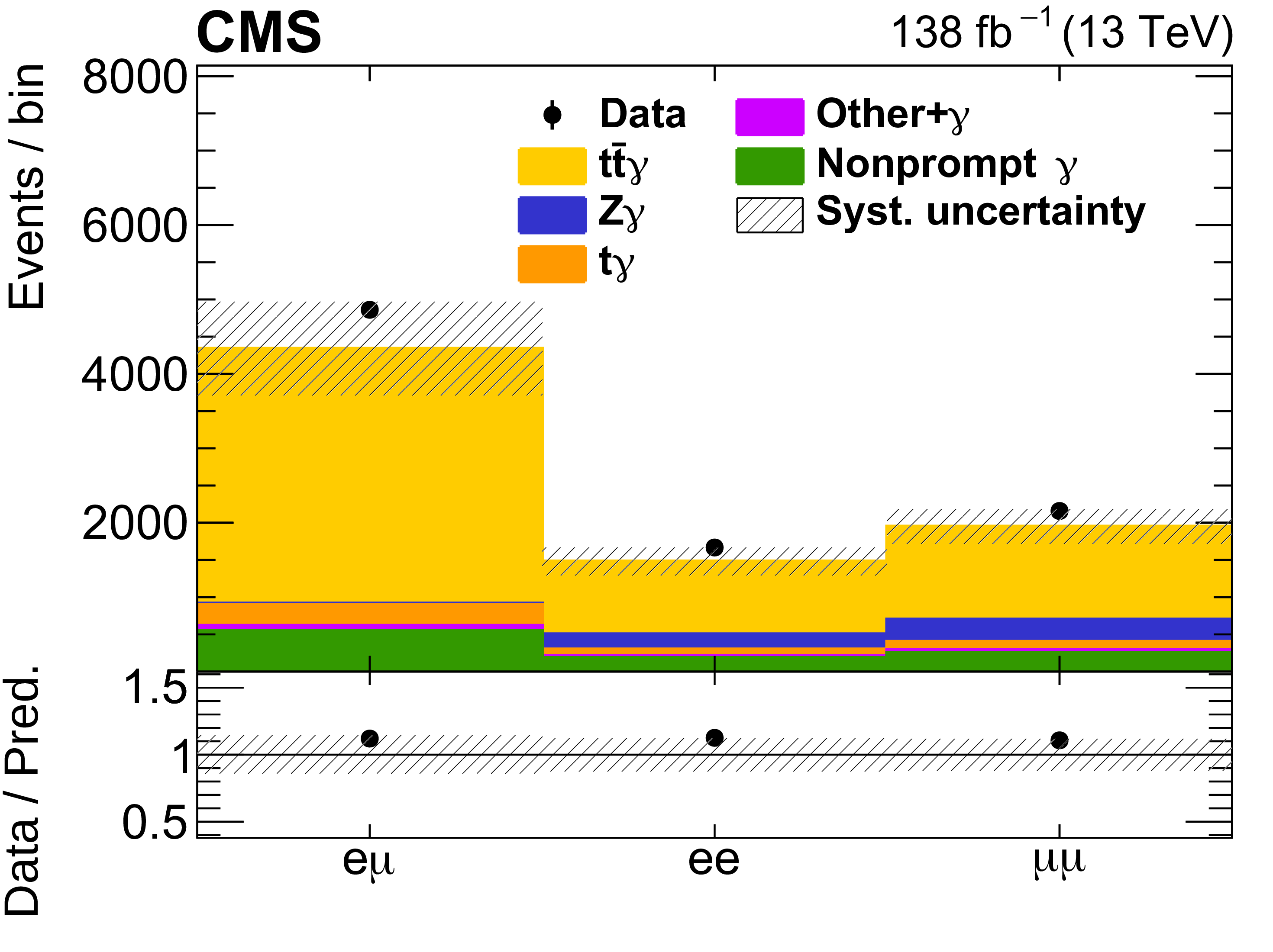
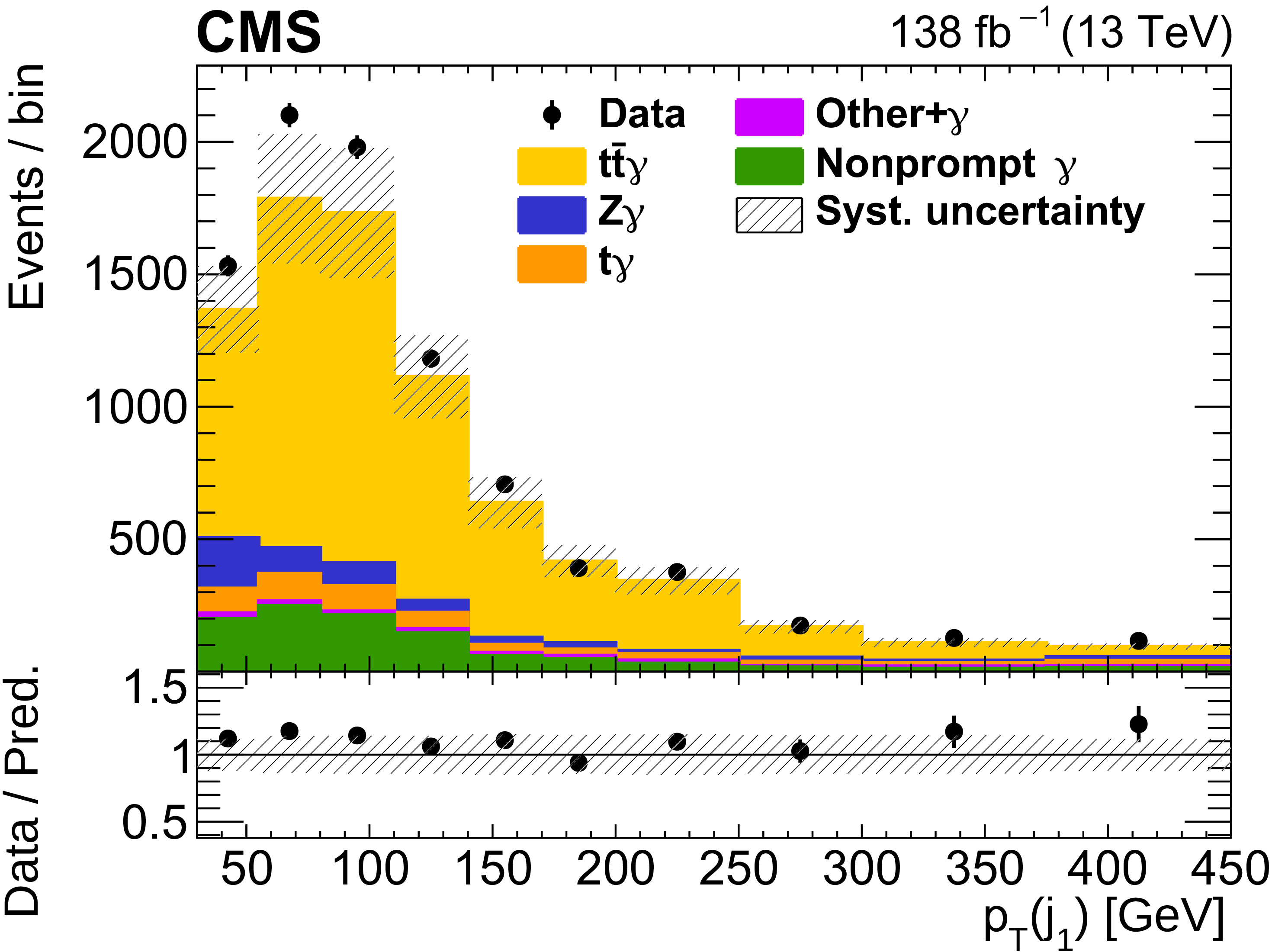
Figure 2:
The observed (points) and predicted (shaded histograms) signal and background yields as functions of the number of jets (upper left) and b-tagged jets (upper right), the ${p_{\mathrm {T}}}$ (middle left) and $| \eta |$ (middle right) of the photon, the dilepton flavours (lower left), and the ${p_{\mathrm {T}}}$ of the leading jet ${\mathrm {j}_1}$ (lower right), after applying the signal selection. Distributions are shown for the three lepton flavour channels combined, with all relevant corrections applied. The predictions are normalized to the expected yields, without taking the results of the fit to the data into account. The vertical bars on the points show the statistical uncertainties in the data, and the hatched bands the systematic uncertainty in the predictions. The lower panels show the ratio of the event yields in data to the overall sum of the predictions. |

png pdf |
Figure 2-a:
The observed (points) and predicted (shaded histograms) signal and background yields as functions of the number of jets, after applying the signal selection. The distribution is shown for the three lepton flavour channels combined, with all relevant corrections applied. The prediction is normalized to the expected yields, without taking the results of the fit to the data into account. The vertical bars on the points show the statistical uncertainties in the data, and the hatched bands the systematic uncertainty in the predictions. The lower panel shows the ratio of the event yields in data to the overall sum of the predictions. |

png pdf |
Figure 2-b:
The observed (points) and predicted (shaded histograms) signal and background yields as functions of the number of b-tagged jets, after applying the signal selection. The distribution is shown for the three lepton flavour channels combined, with all relevant corrections applied. The prediction is normalized to the expected yields, without taking the results of the fit to the data into account. The vertical bars on the points show the statistical uncertainties in the data, and the hatched bands the systematic uncertainty in the predictions. The lower panel shows the ratio of the event yields in data to the overall sum of the predictions. |
png pdf |
Figure 2-c:
The observed (points) and predicted (shaded histograms) signal and background yields as functions of the ${p_{\mathrm {T}}}$ of the photon, after applying the signal selection. The distribution is shown for the three lepton flavour channels combined, with all relevant corrections applied. The prediction is normalized to the expected yields, without taking the results of the fit to the data into account. The vertical bars on the points show the statistical uncertainties in the data, and the hatched bands the systematic uncertainty in the predictions. The lower panel shows the ratio of the event yields in data to the overall sum of the predictions. |
png pdf |
Figure 2-d:
The observed (points) and predicted (shaded histograms) signal and background yields as functions of the $| \eta |$ of the photon, after applying the signal selection. The distribution is shown for the three lepton flavour channels combined, with all relevant corrections applied. The prediction is normalized to the expected yields, without taking the results of the fit to the data into account. The vertical bars on the points show the statistical uncertainties in the data, and the hatched bands the systematic uncertainty in the predictions. The lower panel shows the ratio of the event yields in data to the overall sum of the predictions. |
png pdf |
Figure 2-e:
The observed (points) and predicted (shaded histograms) signal and background yields as functions of the dilepton flavours, after applying the signal selection. The distribution is shown for the three lepton flavour channels combined, with all relevant corrections applied. The prediction is normalized to the expected yields, without taking the results of the fit to the data into account. The vertical bars on the points show the statistical uncertainties in the data, and the hatched bands the systematic uncertainty in the predictions. The lower panel shows the ratio of the event yields in data to the overall sum of the predictions. |
png pdf |
Figure 2-f:
The observed (points) and predicted (shaded histograms) signal and background yields as functions of the ${p_{\mathrm {T}}}$ of the leading jet ${\mathrm {j}_1}$, after applying the signal selection. The distribution is shown for the three lepton flavour channels combined, with all relevant corrections applied. The prediction is normalized to the expected yields, without taking the results of the fit to the data into account. The vertical bars on the points show the statistical uncertainties in the data, and the hatched bands the systematic uncertainty in the predictions. The lower panel shows the ratio of the event yields in data to the overall sum of the predictions. |
png pdf |
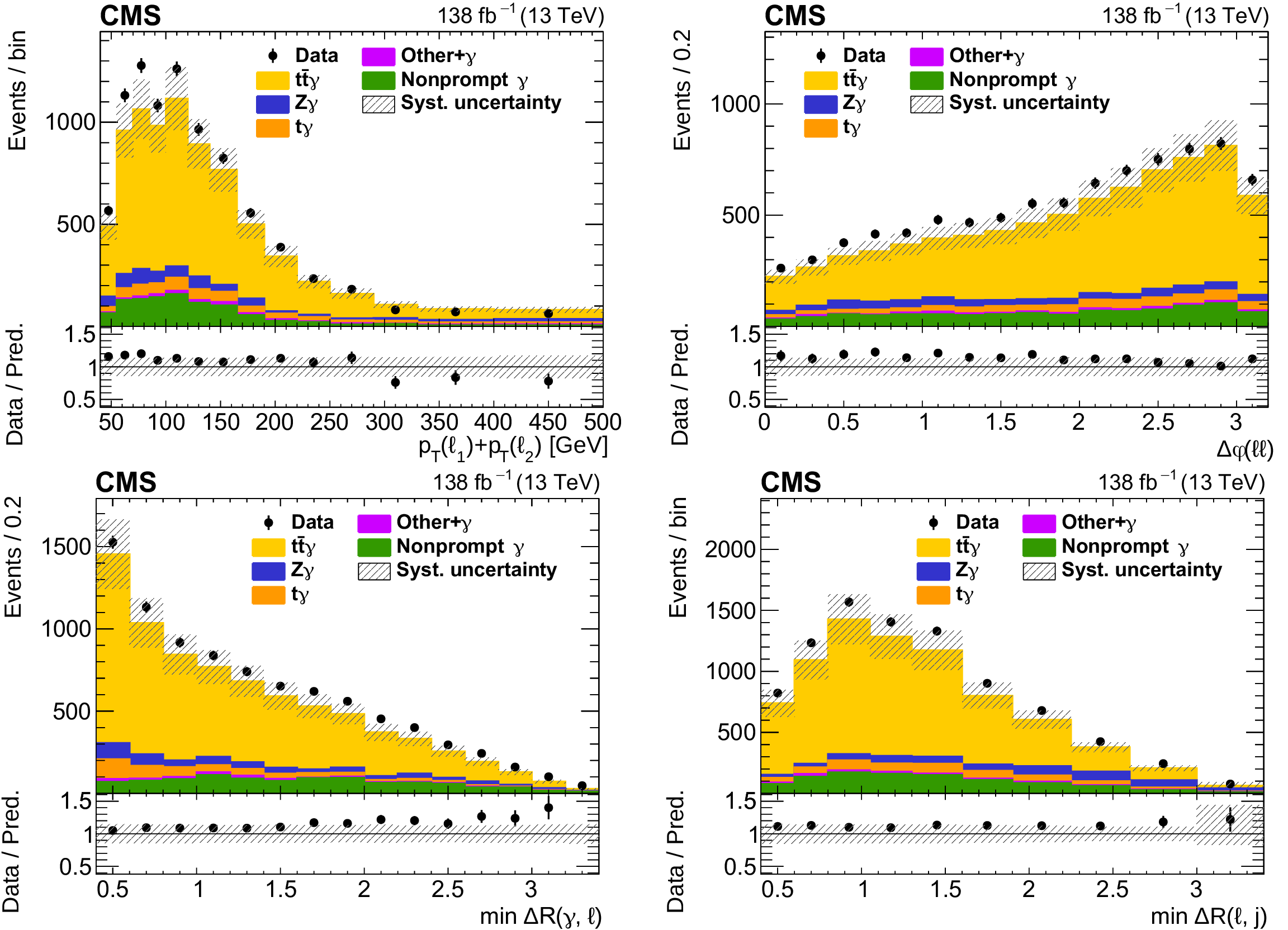
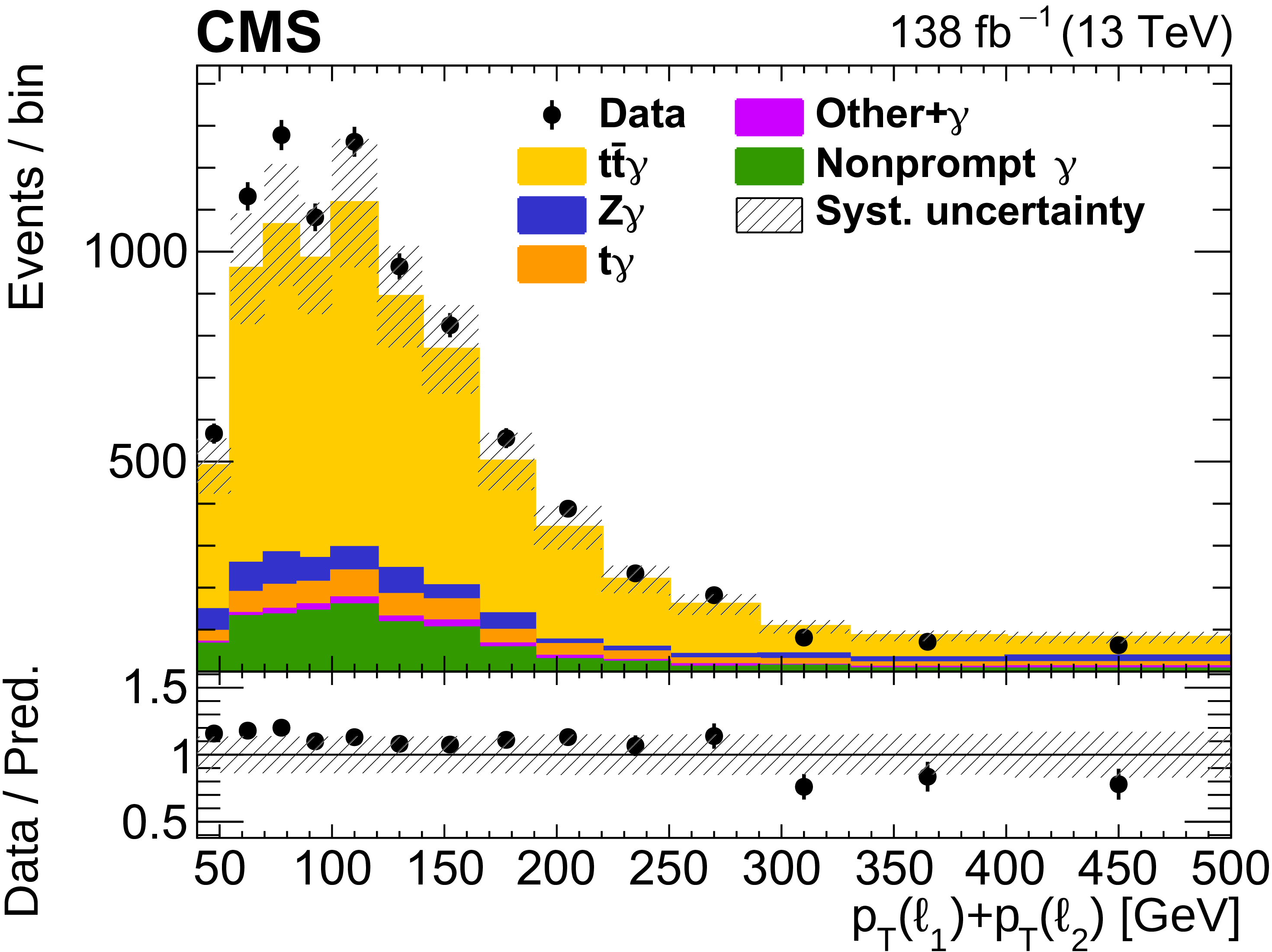
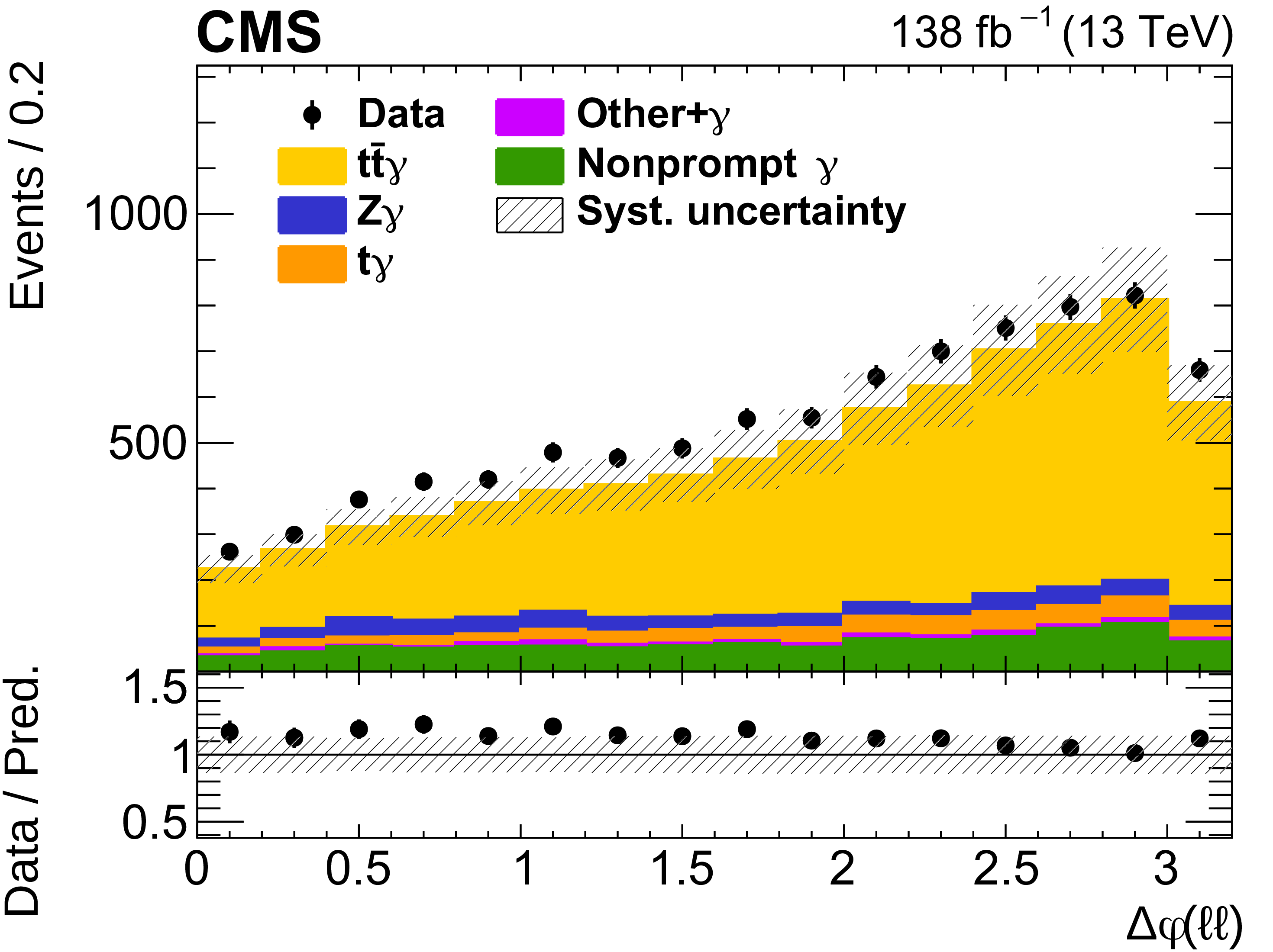
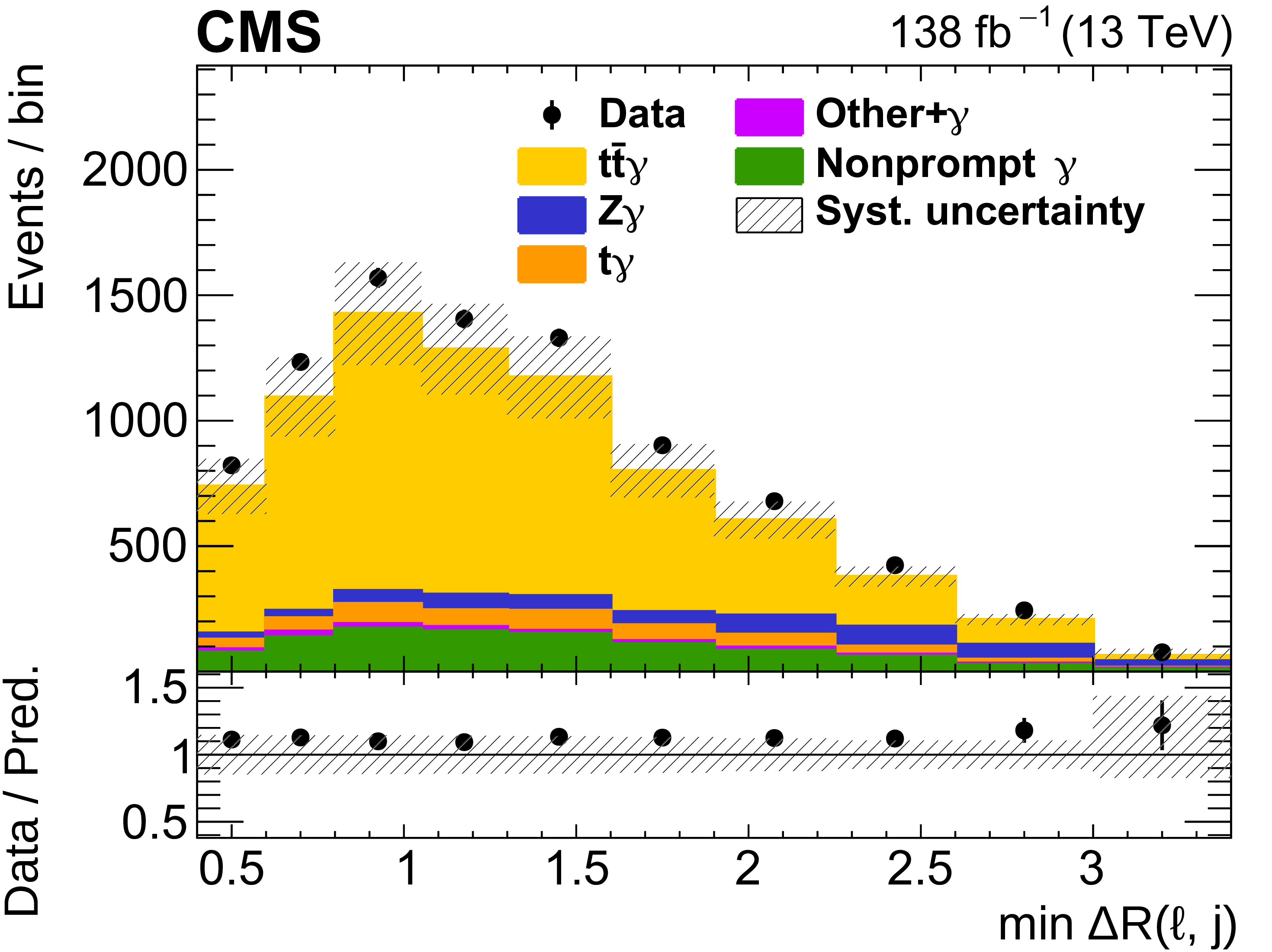
Figure 3:
The observed (points) and predicted (shaded histograms) signal and background yields as functions of the scalar ${p_{\mathrm {T}}}$ sum (upper left) and $\phi $ difference (upper right) of the two leptons, the smallest ${{\Delta R}}$ between the photon and any lepton (lower left), and between any lepton and any jet (lower right), after applying the signal selection. Details can be found in the caption of Fig. 2. |
png pdf |
Figure 3-a:
The observed (points) and predicted (shaded histograms) signal and background yields as functions of the scalar ${p_{\mathrm {T}}}$ sum of the two leptons, after applying the signal selection. Details can be found in the caption of Fig. 2. |
png pdf |
Figure 3-b:
The observed (points) and predicted (shaded histograms) signal and background yields as functions of $\phi $ difference of the two leptons, after applying the signal selection. Details can be found in the caption of Fig. 2. |

png pdf |
Figure 3-c:
The observed (points) and predicted (shaded histograms) signal and background yields as functions of the smallest ${{\Delta R}}$ between the photon and any lepton, after applying the signal selection. Details can be found in the caption of Fig. 2. |
png pdf |
Figure 3-d:
The observed (points) and predicted (shaded histograms) signal and background yields as functions of the smallest ${{\Delta R}}$ between any lepton and any jet, after applying the signal selection. Details can be found in the caption of Fig. 2. |
png pdf |
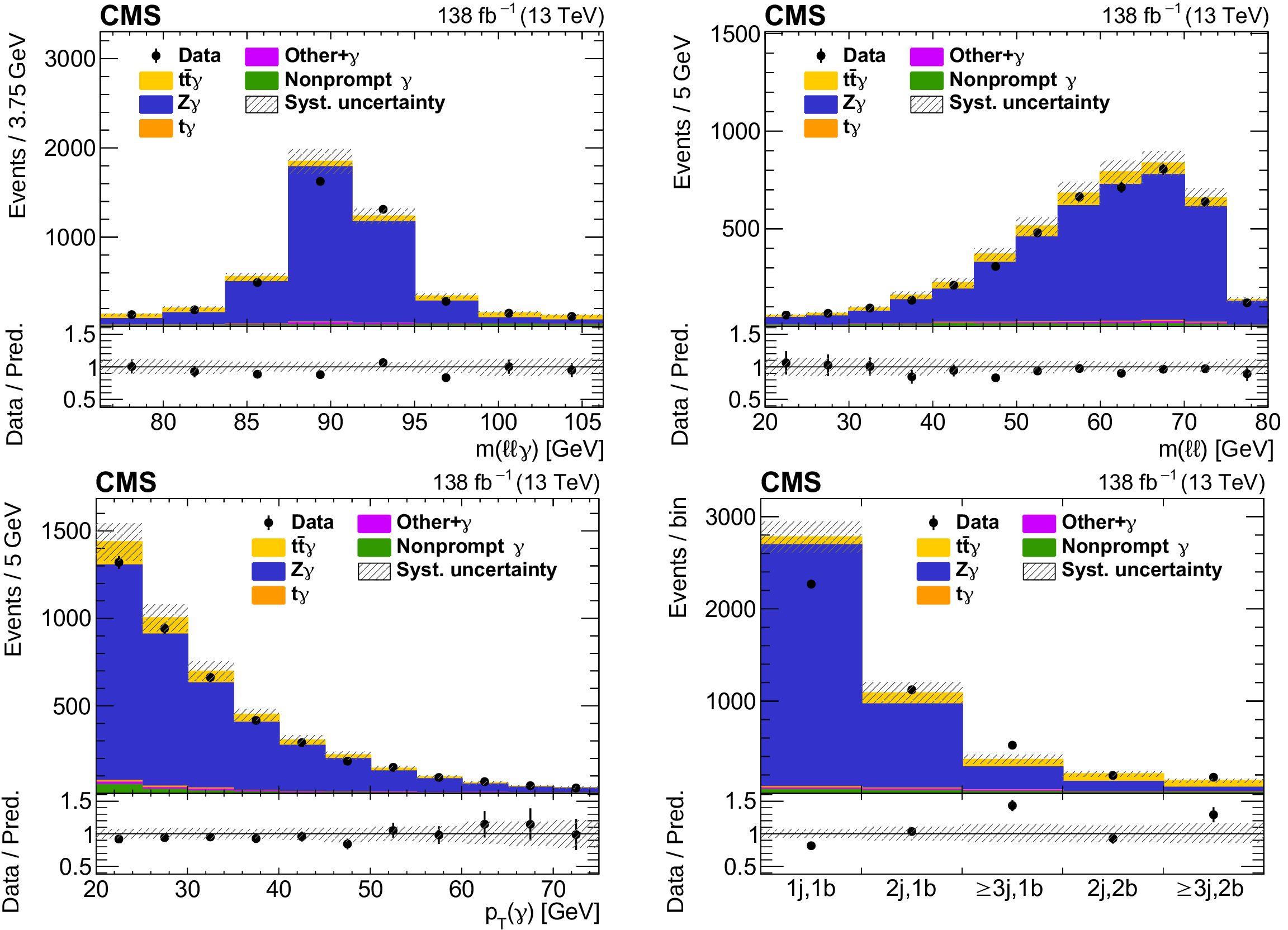
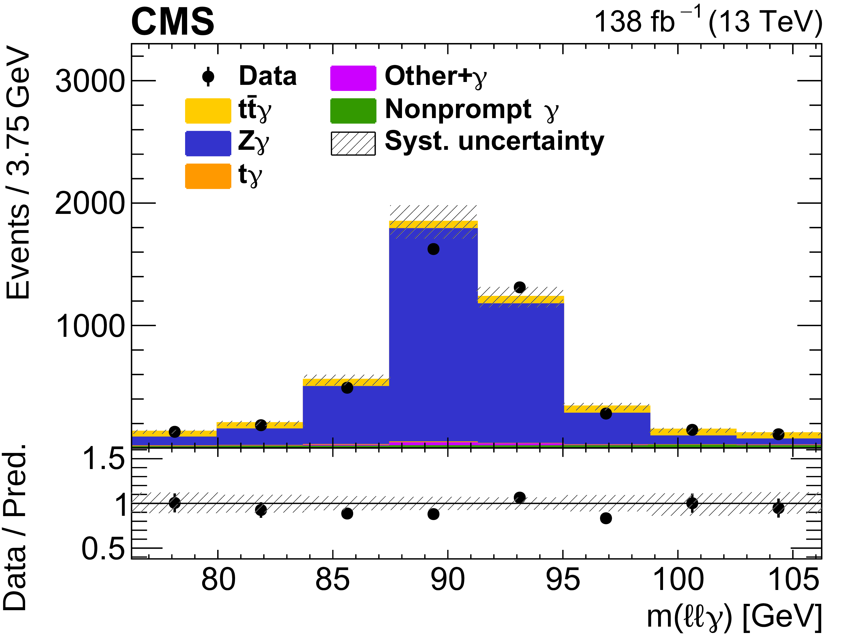
Figure 4:
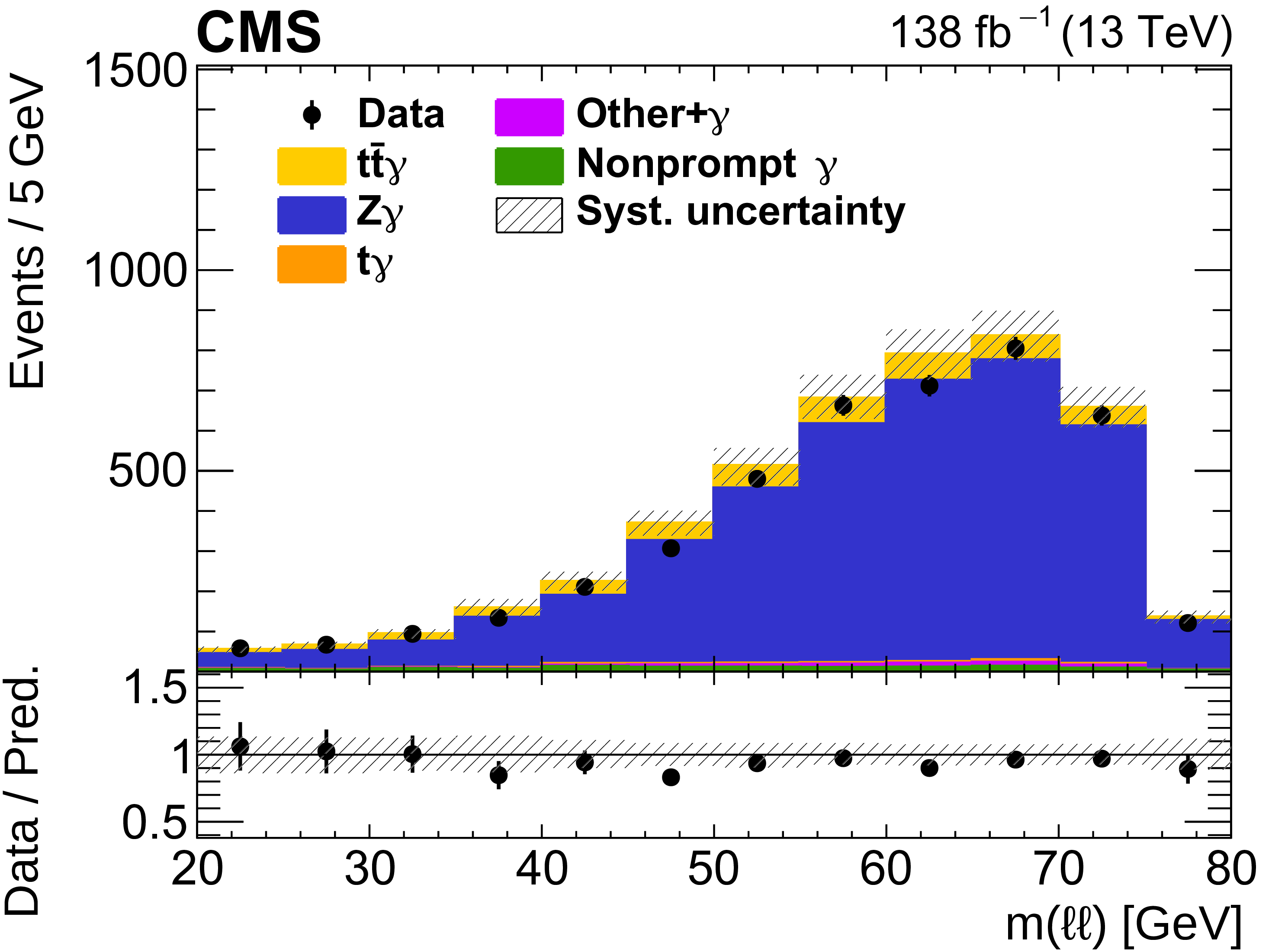
The observed (points) and predicted (shaded histograms) event yields as a function of ${m(\ell \ell \gamma)}$ (upper left), ${m(\ell \ell)}$ (upper right), photon ${p_{\mathrm {T}}}$ (lower left), and the number of jets j and b-tagged jets b (lower right), after applying the event selection for the Z$ \gamma$ control region. The vertical lines on the points show the statistical uncertainties in the data, and the hatched bands the systematic uncertainty in the predictions. The lower panels show the ratio of the event yields in data to the sum of the predictions. |
png pdf |
Figure 4-a:
The observed (points) and predicted (shaded histograms) event yields as a function of ${m(\ell \ell \gamma)}$, after applying the event selection for the Z$ \gamma$ control region. The vertical lines on the points show the statistical uncertainties in the data, and the hatched bands the systematic uncertainty in the predictions. The lower panel shows the ratio of the event yields in data to the sum of the predictions. |
png pdf |
Figure 4-b:
The observed (points) and predicted (shaded histograms) event yields as a function of ${m(\ell \ell)}$, after applying the event selection for the Z$ \gamma$ control region. The vertical lines on the points show the statistical uncertainties in the data, and the hatched bands the systematic uncertainty in the predictions. The lower panel shows the ratio of the event yields in data to the sum of the predictions. |

png pdf |
Figure 4-c:
The observed (points) and predicted (shaded histograms) event yields as a function of photon ${p_{\mathrm {T}}}$, after applying the event selection for the Z$ \gamma$ control region. The vertical lines on the points show the statistical uncertainties in the data, and the hatched bands the systematic uncertainty in the predictions. The lower panel shows the ratio of the event yields in data to the sum of the predictions. |

png pdf |
Figure 4-d:
The observed (points) and predicted (shaded histograms) event yields as a function of the number of jets j and b-tagged jets b, after applying the event selection for the Z$ \gamma$ control region. The vertical lines on the points show the statistical uncertainties in the data, and the hatched bands the systematic uncertainty in the predictions. The lower panel shows the ratio of the event yields in data to the sum of the predictions. |
png pdf |
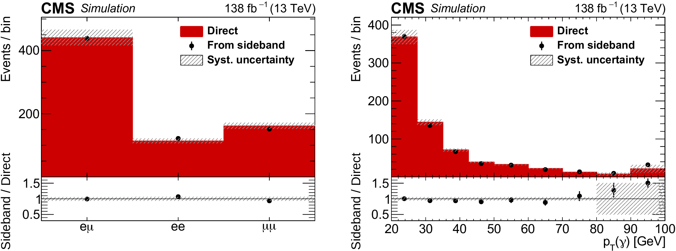
Figure 5:
Event yields in the signal region predicted from a simulated ${\mathrm{t} \mathrm{\bar{t}}}$ event sample (shaded histogram) and estimated from applying the transfer factor to the event yields of the same sample in the sideband region (points), as a function of the lepton flavour (left) and the photon ${p_{\mathrm {T}}}$ (right). The vertical lines on the points show the statistical uncertainties from the simulated event samples, and the hatched bands the total systematic uncertainty assigned to the nonprompt-photon background estimate. The lower panels show the ratio of the two predictions. |

png pdf |
Figure 5-a:
Event yields in the signal region predicted from a simulated ${\mathrm{t} \mathrm{\bar{t}}}$ event sample (shaded histogram) and estimated from applying the transfer factor to the event yields of the same sample in the sideband region (points), as a function of the lepton flavour. The vertical lines on the points show the statistical uncertainties from the simulated event samples, and the hatched bands the total systematic uncertainty assigned to the nonprompt-photon background estimate. The lower panel shows the ratio of the two predictions. |

png pdf |
Figure 5-b:
Event yields in the signal region predicted from a simulated ${\mathrm{t} \mathrm{\bar{t}}}$ event sample (shaded histogram) and estimated from applying the transfer factor to the event yields of the same sample in the sideband region (points), as a function of the photon ${p_{\mathrm {T}}}$. The vertical lines on the points show the statistical uncertainties from the simulated event samples, and the hatched bands the total systematic uncertainty assigned to the nonprompt-photon background estimate. The lower panel shows the ratio of the two predictions. |

png pdf |
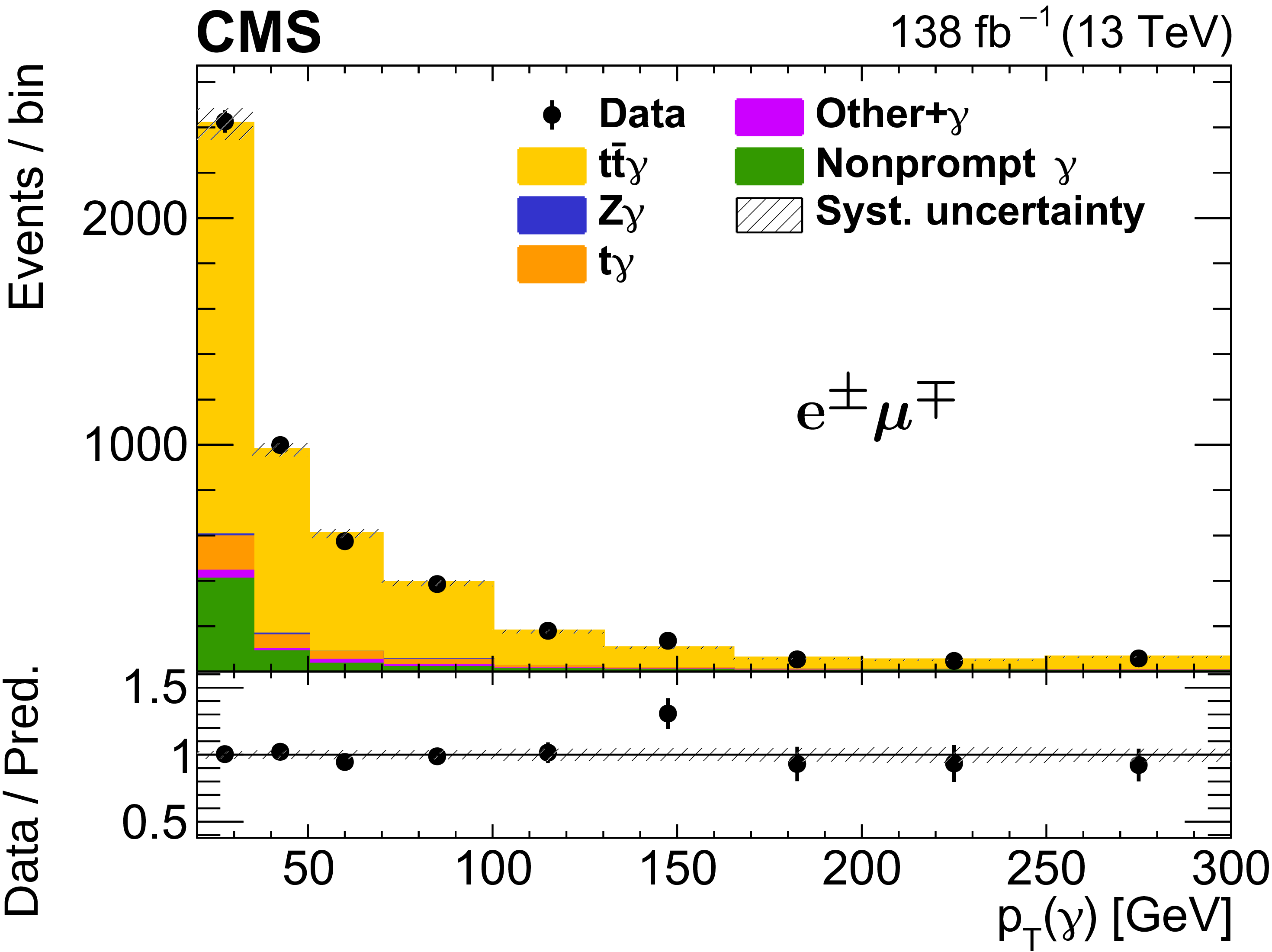
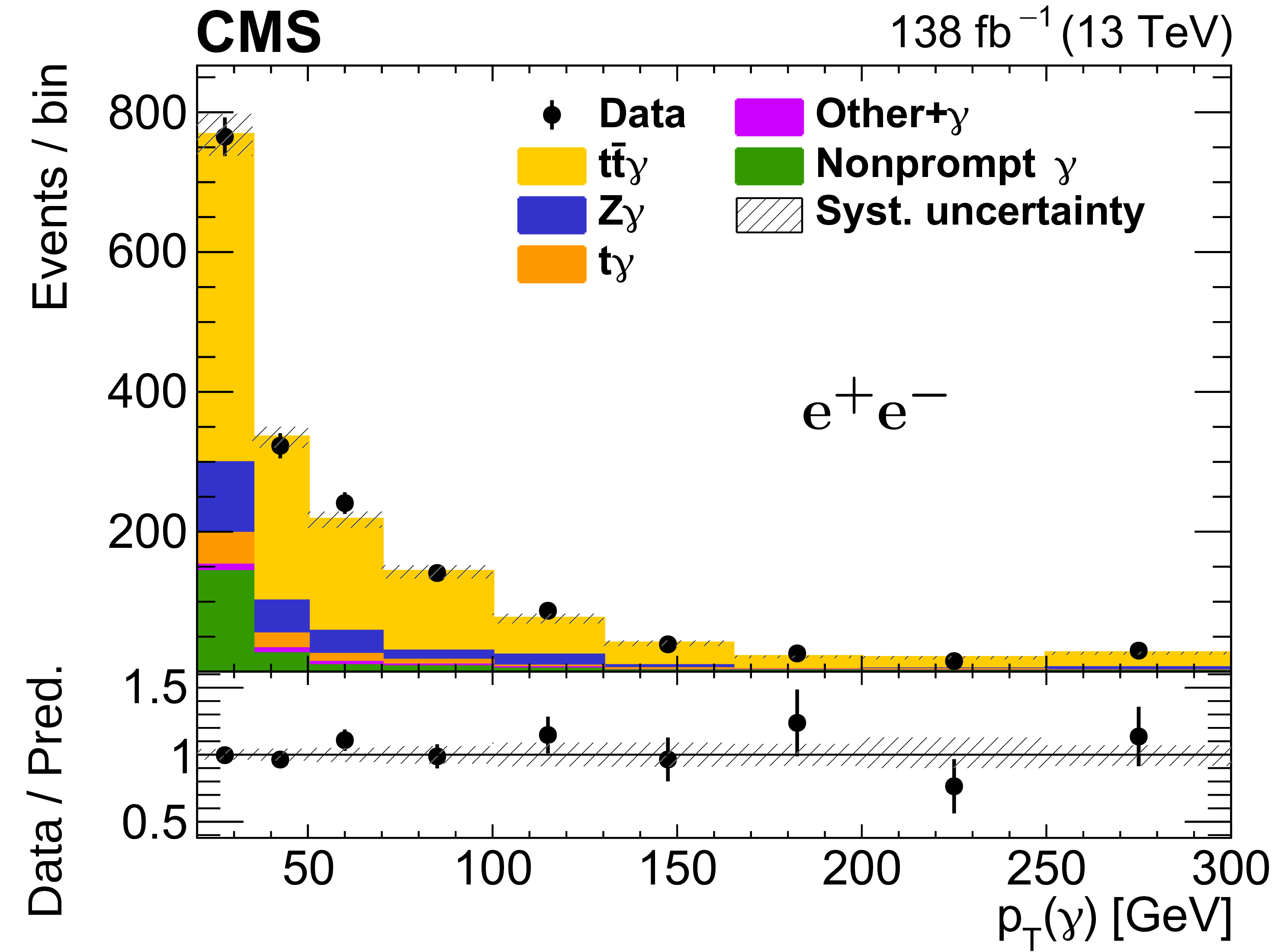
Figure 6:
The observed (points) and predicted (shaded histograms) event yields as a function of the reconstructed photon ${p_{\mathrm {T}}}$ after applying the signal selection, for the ${\mathrm{e^{\pm}} {\mu ^\mp}}$ (upper left), ${\mathrm{e^{+}} \mathrm{e^{-}}}$ (upper right), and ${\mu^{+} \mu^{-}}$ (lower) channels, after the values of the normalizations and nuisance parameters obtained in the fit to the data are applied. The vertical bars on the points show the statistical uncertainties in data, and the hatched bands the systematic uncertainty in the predictions. The lower panels of each plot show the ratio of the event yields in data to the predictions. |
png pdf |
Figure 6-a:
The observed (points) and predicted (shaded histograms) event yields as a function of the reconstructed photon ${p_{\mathrm {T}}}$ after applying the signal selection, for the ${\mathrm{e^{\pm}} {\mu ^\mp}}$ channel, after the values of the normalizations and nuisance parameters obtained in the fit to the data are applied. The vertical bars on the points show the statistical uncertainties in data, and the hatched bands the systematic uncertainty in the predictions. The lower panel shows the ratio of the event yields in data to the predictions. |
png pdf |
Figure 6-b:
The observed (points) and predicted (shaded histograms) event yields as a function of the reconstructed photon ${p_{\mathrm {T}}}$ after applying the signal selection, for the ${\mathrm{e^{+}} \mathrm{e^{-}}}$ channel, after the values of the normalizations and nuisance parameters obtained in the fit to the data are applied. The vertical bars on the points show the statistical uncertainties in data, and the hatched bands the systematic uncertainty in the predictions. The lower panel shows the ratio of the event yields in data to the predictions. |

png pdf |
Figure 6-c:
The observed (points) and predicted (shaded histograms) event yields as a function of the reconstructed photon ${p_{\mathrm {T}}}$ after applying the signal selection, for the ${\mu^{+} \mu^{-}}$ channel, after the values of the normalizations and nuisance parameters obtained in the fit to the data are applied. The vertical bars on the points show the statistical uncertainties in data, and the hatched bands the systematic uncertainty in the predictions. The lower panel shows the ratio of the event yields in data to the predictions. |
png pdf |
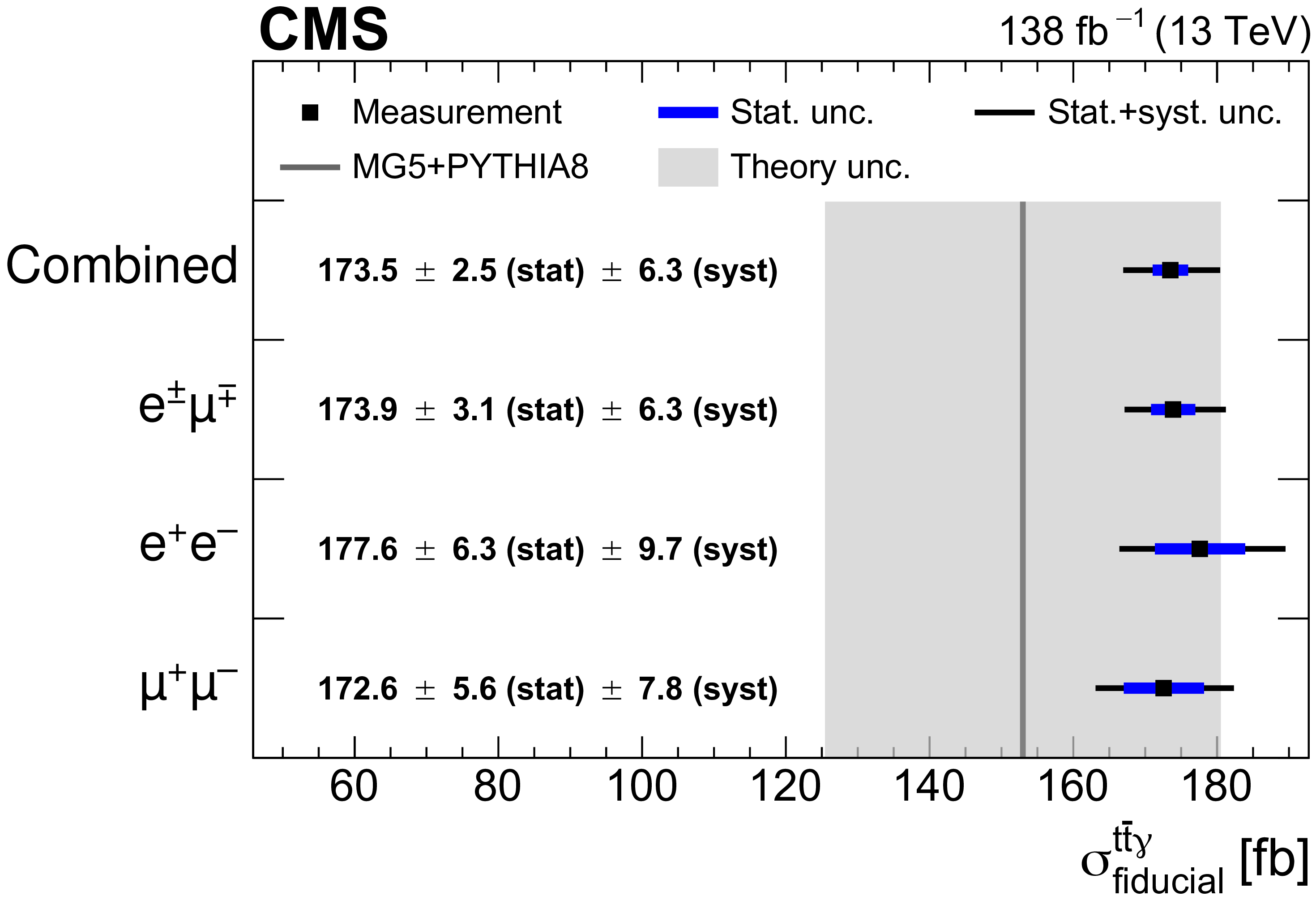
Figure 7:
The measured inclusive fiducial ${{\mathrm{t} \mathrm{\bar{t}}} \gamma}$ production cross section in the dilepton final state for the different dilepton-flavour channels and combined. The thick and thin lines on the points show the statistical and total uncertainties, respectively. The vertical line represents the SM prediction obtained with the MadGraph 5\_aMC@NLO (MG5) interfaced with PYTHIA 8, as described in the text. The shaded band shows the theoretical uncertainty in the prediction. |

png pdf |
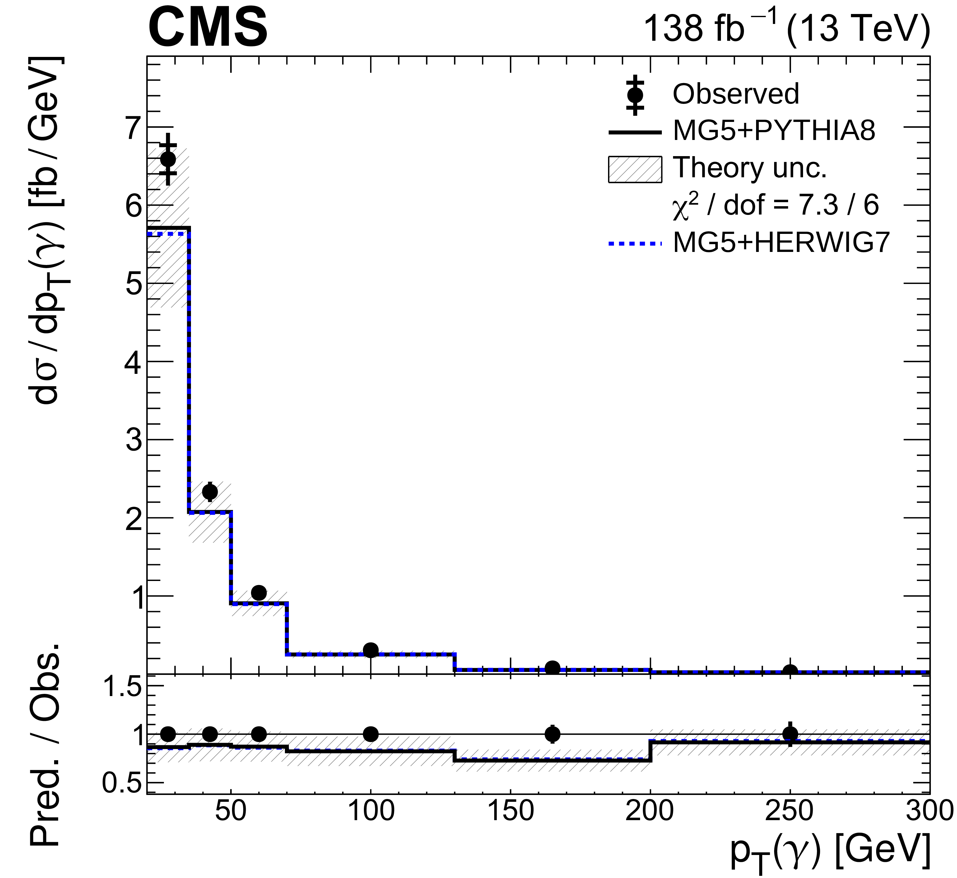
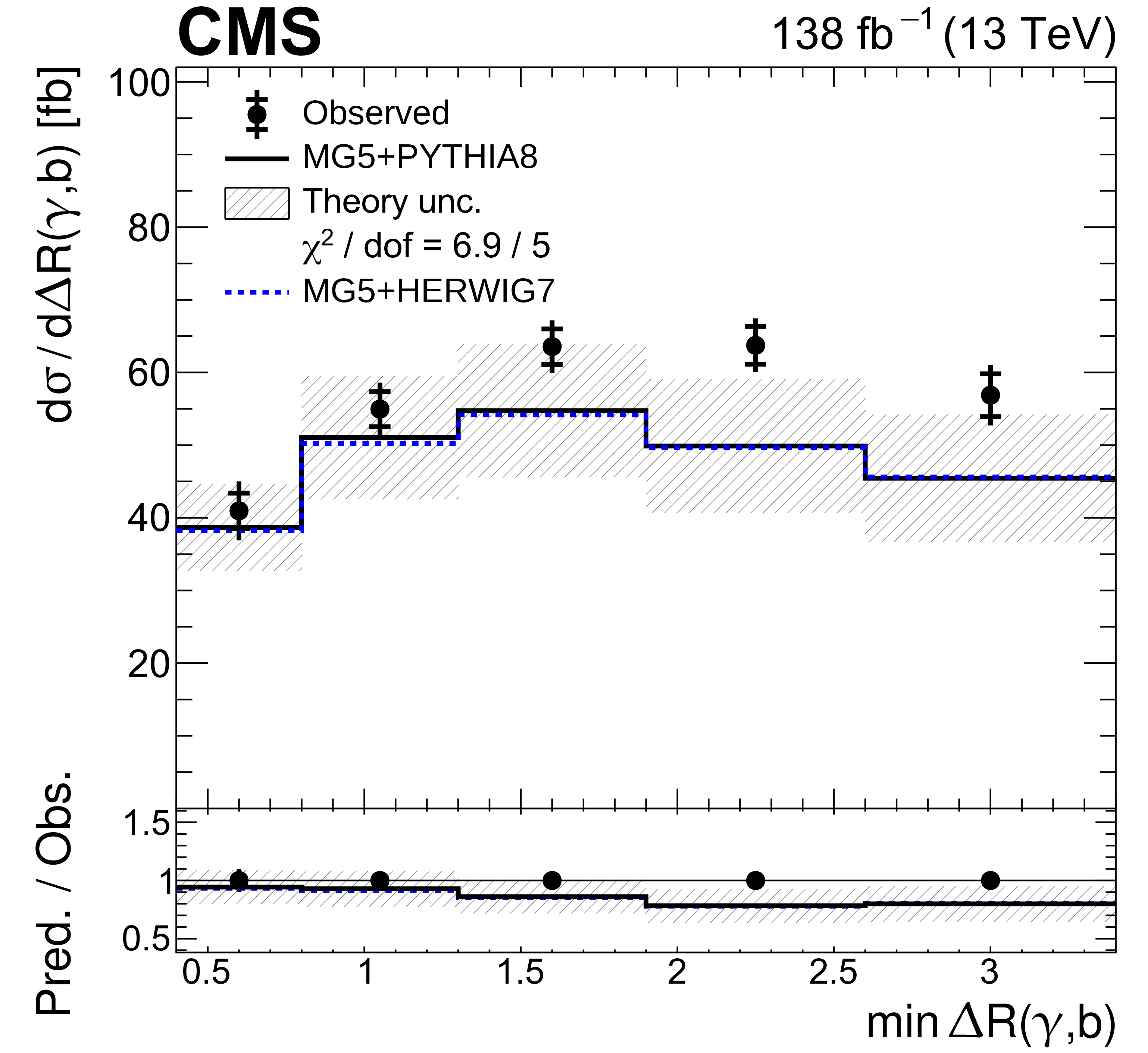
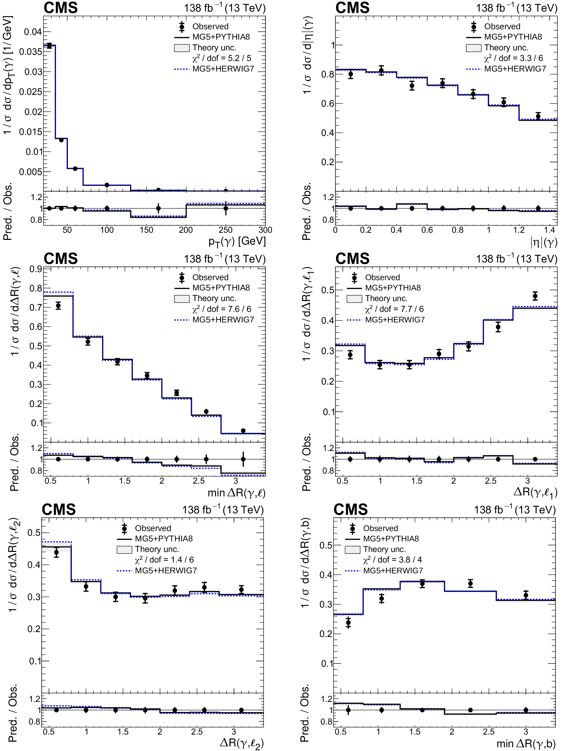
Figure 8:
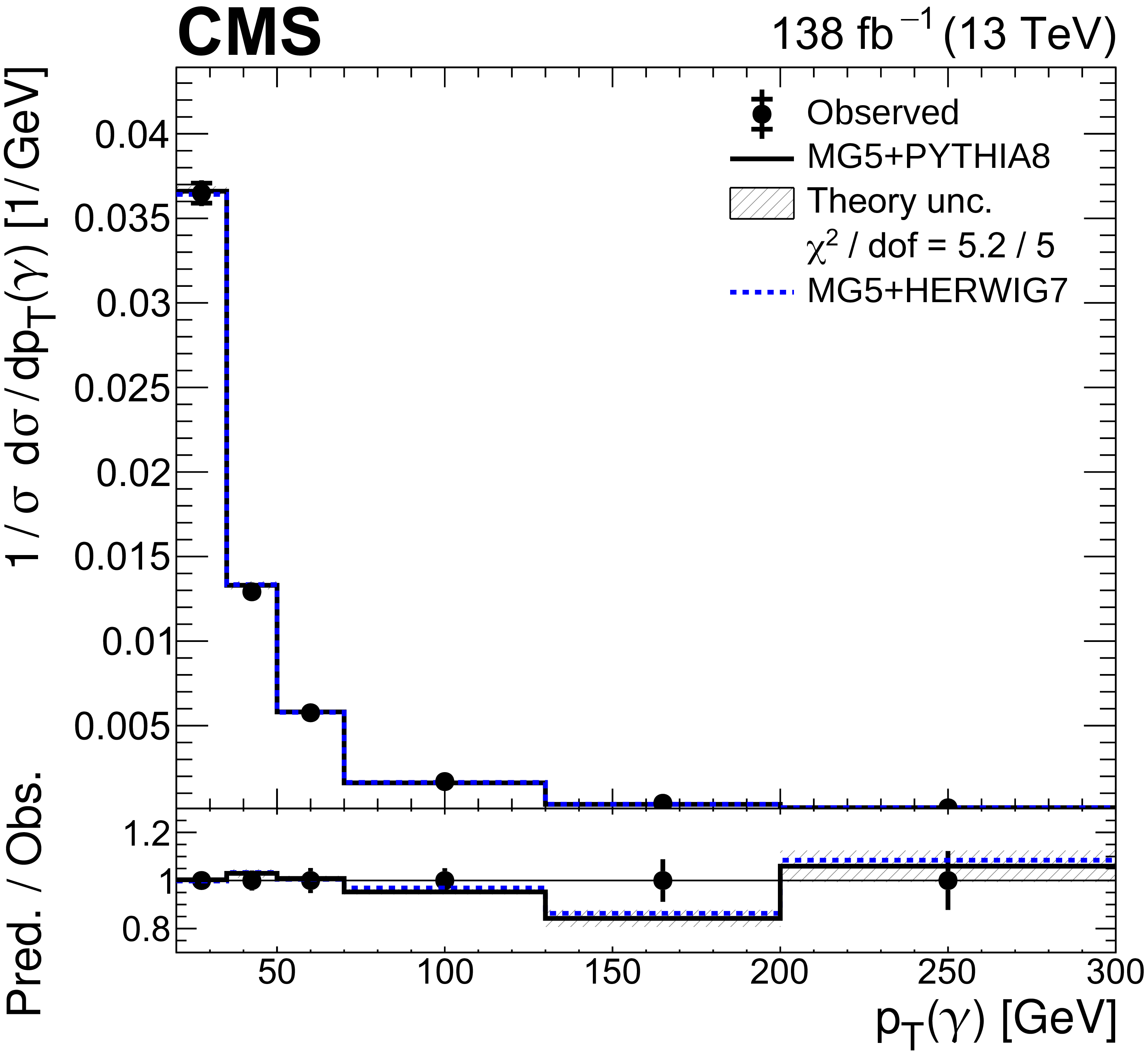
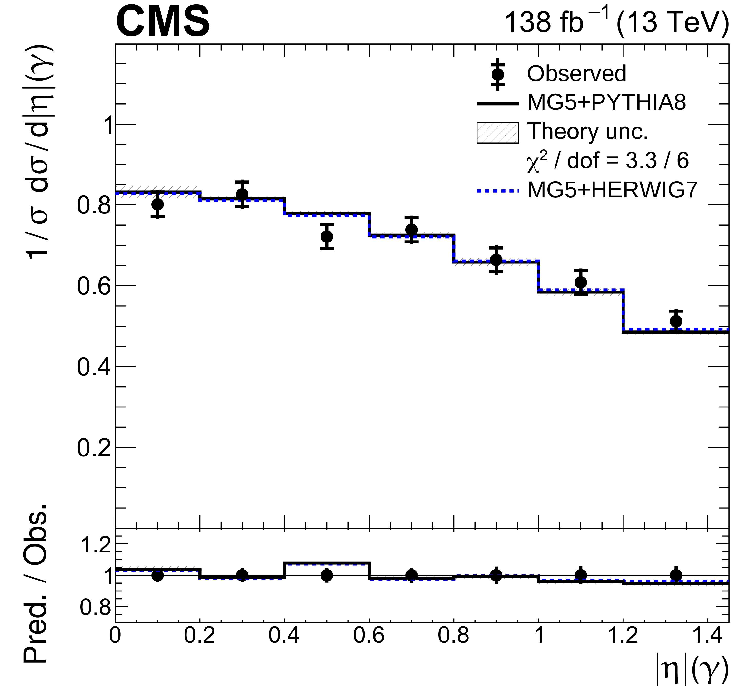
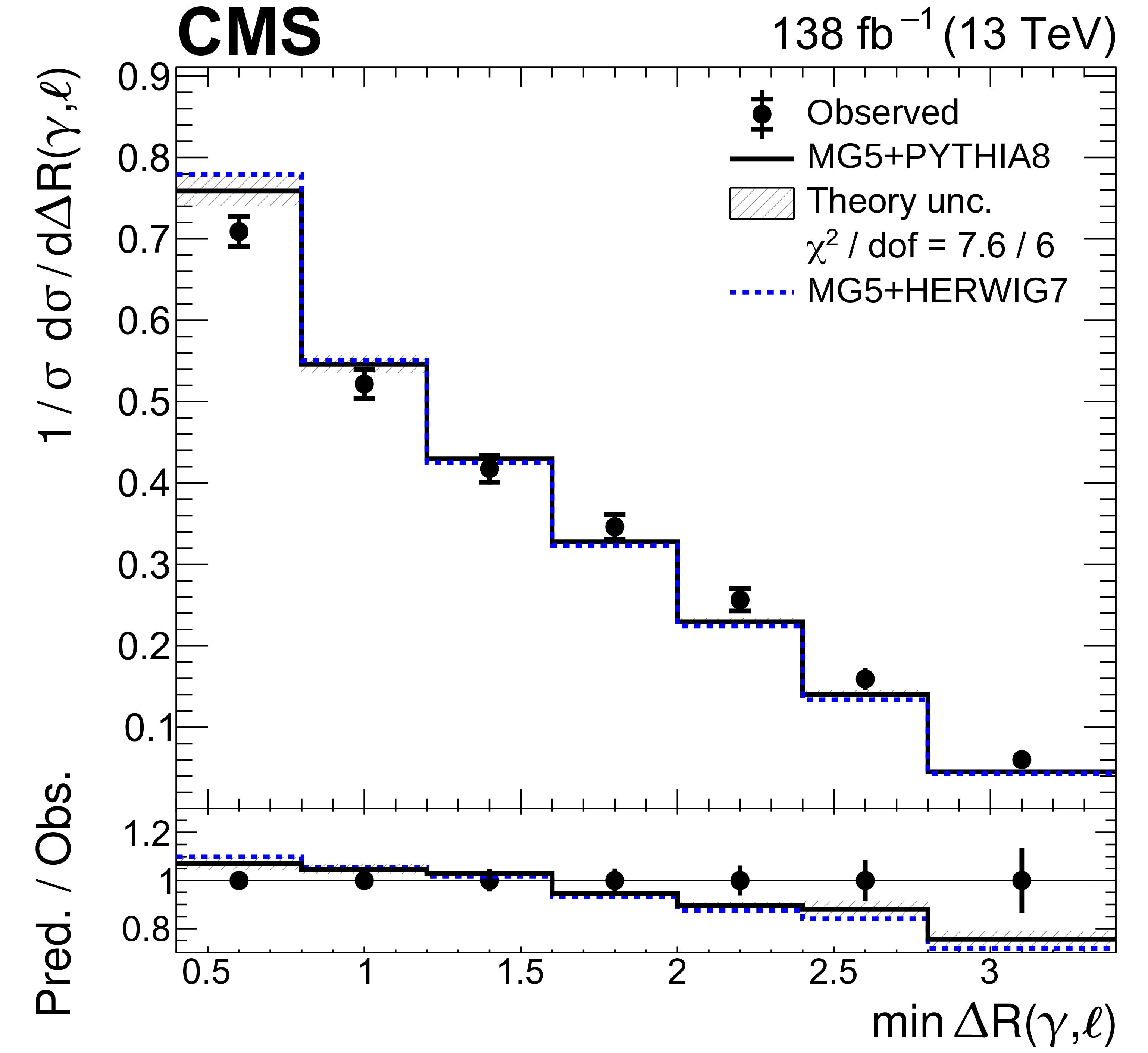
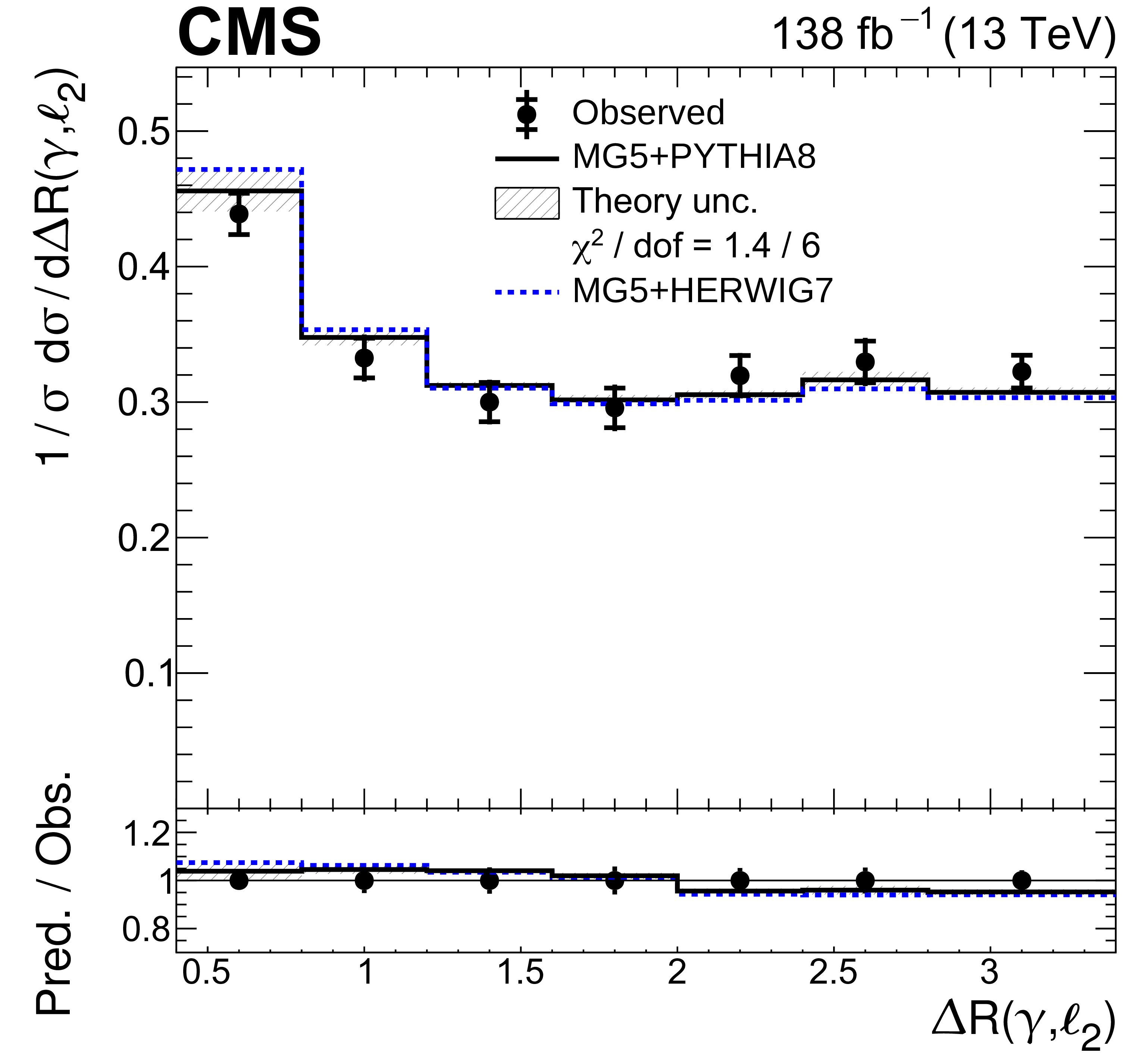
Absolute differential ${{\mathrm{t} \mathrm{\bar{t}}} \gamma}$ production cross sections as functions of ${{p_{\mathrm {T}}} (\gamma)}$ (upper left), ${{{| \eta |}} (\gamma)}$ (upper right), ${\min {{{\Delta R}} (\gamma,\ell)}}$ (middle left), ${{{\Delta R}} (\gamma,\ell _1)}$ (middle right), ${{{\Delta R}} (\gamma,\ell _2)}$ (lower left), and ${\min {{\Delta R}} (\gamma,\mathrm{b})}$ (lower right). The data are represented by points, with inner (outer) vertical bars indicating the statistical (total) uncertainties. The predictions obtained with the MadGraph 5\_aMC@NLO event generator interfaced with PYTHIA 8 (solid lines) and HERWIG 7 (dotted lines) parton shower simulations are shown as horizontal lines. The theoretical uncertainties in the prediction using PYTHIA 8 are indicated by shaded bands. The lower panels display the ratios of the predictions to the measurement. The values of the ${\chi ^2}$ divided by the number of degrees of freedom (dof) quantifying the agreement between the measurement and the prediction using PYTHIA 8 are indicated in the legends. |
png pdf |
Figure 8-a:
Absolute differential ${{\mathrm{t} \mathrm{\bar{t}}} \gamma}$ production cross sections as functions of ${{p_{\mathrm {T}}} (\gamma)}$. The data are represented by points, with inner (outer) vertical bars indicating the statistical (total) uncertainties. The predictions obtained with the MadGraph 5\_aMC@NLO event generator interfaced with PYTHIA 8 (solid lines) and HERWIG 7 (dotted lines) parton shower simulations are shown as horizontal lines. The theoretical uncertainties in the prediction using PYTHIA 8 are indicated by shaded bands. The lower panel displays the ratios of the predictions to the measurement. The values of the ${\chi ^2}$ divided by the number of degrees of freedom (dof) quantifying the agreement between the measurement and the prediction using PYTHIA 8 are indicated in the legends. |

png pdf |
Figure 8-b:
Absolute differential ${{\mathrm{t} \mathrm{\bar{t}}} \gamma}$ production cross sections as functions of ${{{| \eta |}} (\gamma)}$. The data are represented by points, with inner (outer) vertical bars indicating the statistical (total) uncertainties. The predictions obtained with the MadGraph 5\_aMC@NLO event generator interfaced with PYTHIA 8 (solid lines) and HERWIG 7 (dotted lines) parton shower simulations are shown as horizontal lines. The theoretical uncertainties in the prediction using PYTHIA 8 are indicated by shaded bands. The lower panel displays the ratios of the predictions to the measurement. The values of the ${\chi ^2}$ divided by the number of degrees of freedom (dof) quantifying the agreement between the measurement and the prediction using PYTHIA 8 are indicated in the legends. |

png pdf |
Figure 8-c:
Absolute differential ${{\mathrm{t} \mathrm{\bar{t}}} \gamma}$ production cross sections as functions of ${\min {{{\Delta R}} (\gamma,\ell)}}$. The data are represented by points, with inner (outer) vertical bars indicating the statistical (total) uncertainties. The predictions obtained with the MadGraph 5\_aMC@NLO event generator interfaced with PYTHIA 8 (solid lines) and HERWIG 7 (dotted lines) parton shower simulations are shown as horizontal lines. The theoretical uncertainties in the prediction using PYTHIA 8 are indicated by shaded bands. The lower panel displays the ratios of the predictions to the measurement. The values of the ${\chi ^2}$ divided by the number of degrees of freedom (dof) quantifying the agreement between the measurement and the prediction using PYTHIA 8 are indicated in the legends. |

png pdf |
Figure 8-d:
Absolute differential ${{\mathrm{t} \mathrm{\bar{t}}} \gamma}$ production cross sections as functions of ${{{\Delta R}} (\gamma,\ell _1)}$. The data are represented by points, with inner (outer) vertical bars indicating the statistical (total) uncertainties. The predictions obtained with the MadGraph 5\_aMC@NLO event generator interfaced with PYTHIA 8 (solid lines) and HERWIG 7 (dotted lines) parton shower simulations are shown as horizontal lines. The theoretical uncertainties in the prediction using PYTHIA 8 are indicated by shaded bands. The lower panel displays the ratios of the predictions to the measurement. The values of the ${\chi ^2}$ divided by the number of degrees of freedom (dof) quantifying the agreement between the measurement and the prediction using PYTHIA 8 are indicated in the legends. |

png pdf |
Figure 8-e:
Absolute differential ${{\mathrm{t} \mathrm{\bar{t}}} \gamma}$ production cross sections as functions of ${{{\Delta R}} (\gamma,\ell _2)}$. The data are represented by points, with inner (outer) vertical bars indicating the statistical (total) uncertainties. The predictions obtained with the MadGraph 5\_aMC@NLO event generator interfaced with PYTHIA 8 (solid lines) and HERWIG 7 (dotted lines) parton shower simulations are shown as horizontal lines. The theoretical uncertainties in the prediction using PYTHIA 8 are indicated by shaded bands. The lower panel displays the ratios of the predictions to the measurement. The values of the ${\chi ^2}$ divided by the number of degrees of freedom (dof) quantifying the agreement between the measurement and the prediction using PYTHIA 8 are indicated in the legends. |
png pdf |
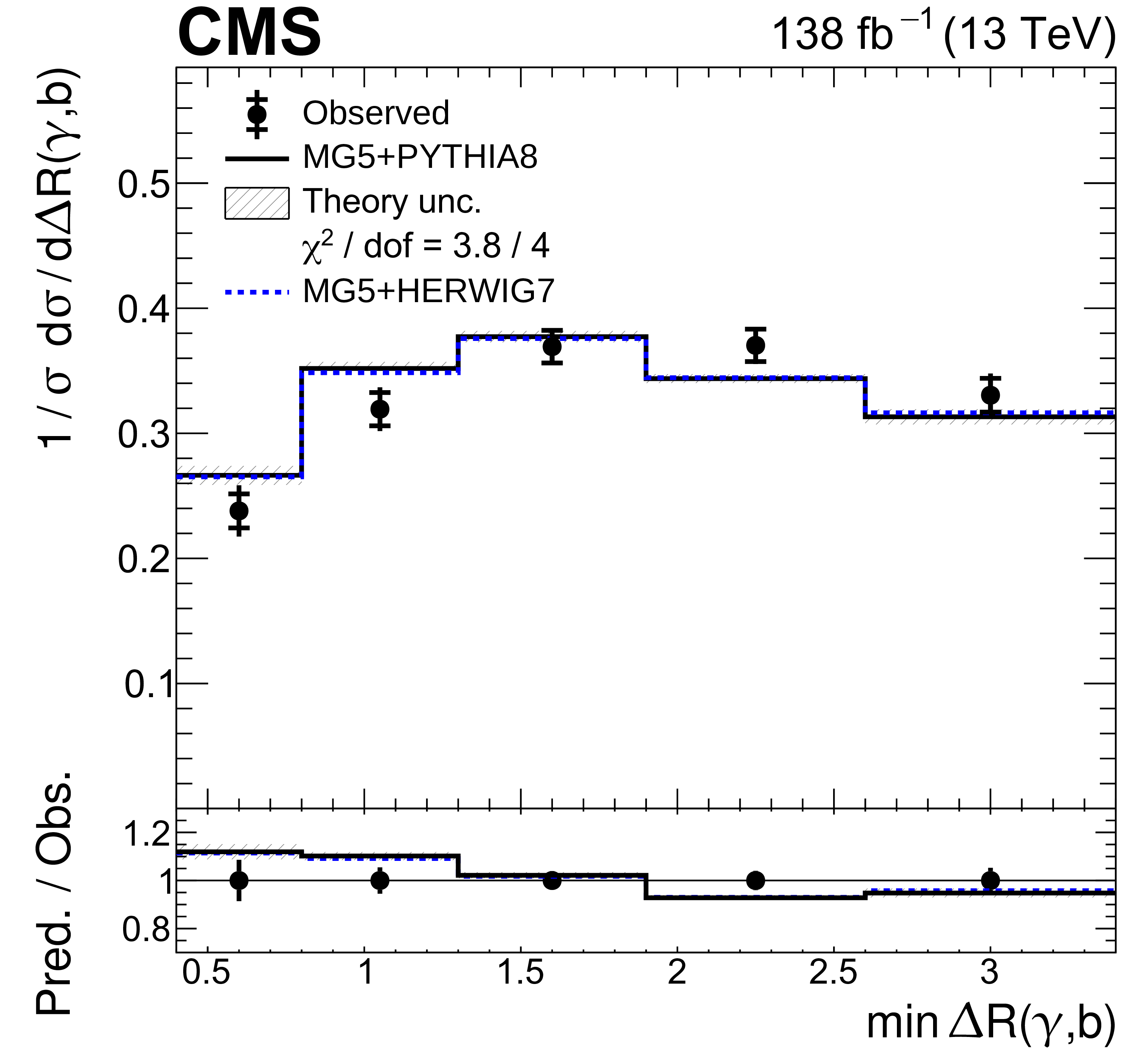
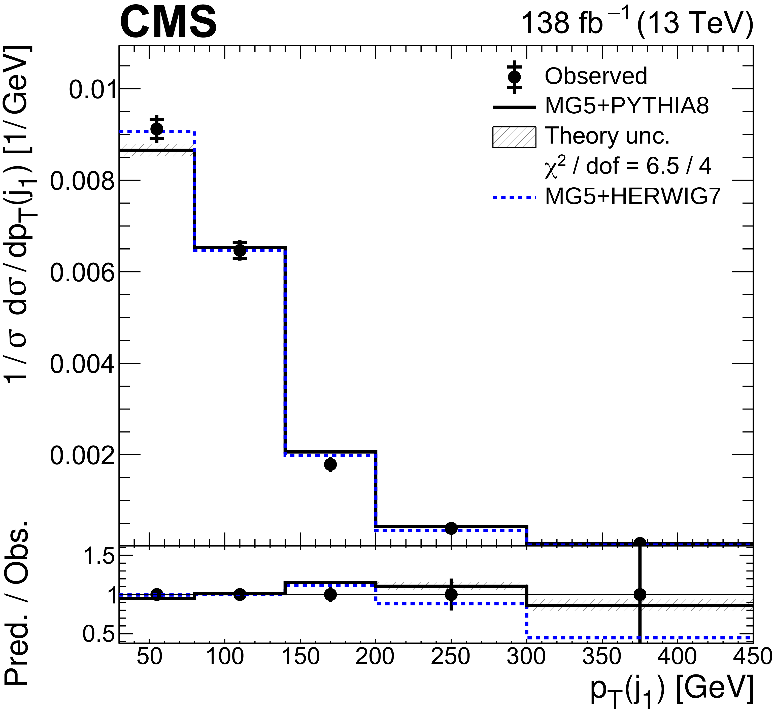
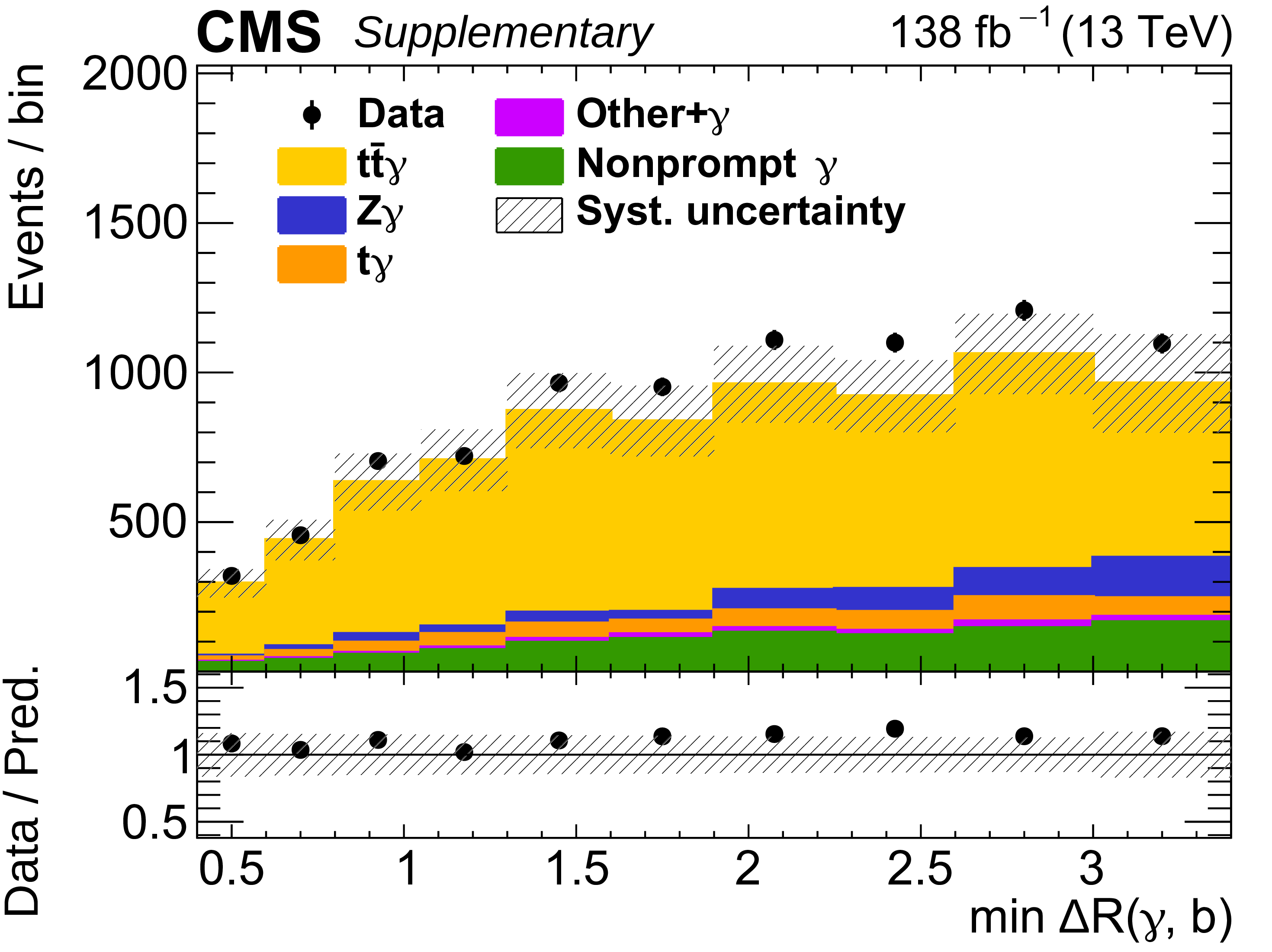
Figure 8-f:
Absolute differential ${{\mathrm{t} \mathrm{\bar{t}}} \gamma}$ production cross sections as functions of ${\min {{\Delta R}} (\gamma,\mathrm{b})}$. The data are represented by points, with inner (outer) vertical bars indicating the statistical (total) uncertainties. The predictions obtained with the MadGraph 5\_aMC@NLO event generator interfaced with PYTHIA 8 (solid lines) and HERWIG 7 (dotted lines) parton shower simulations are shown as horizontal lines. The theoretical uncertainties in the prediction using PYTHIA 8 are indicated by shaded bands. The lower panel displays the ratios of the predictions to the measurement. The values of the ${\chi ^2}$ divided by the number of degrees of freedom (dof) quantifying the agreement between the measurement and the prediction using PYTHIA 8 are indicated in the legends. |
png pdf |
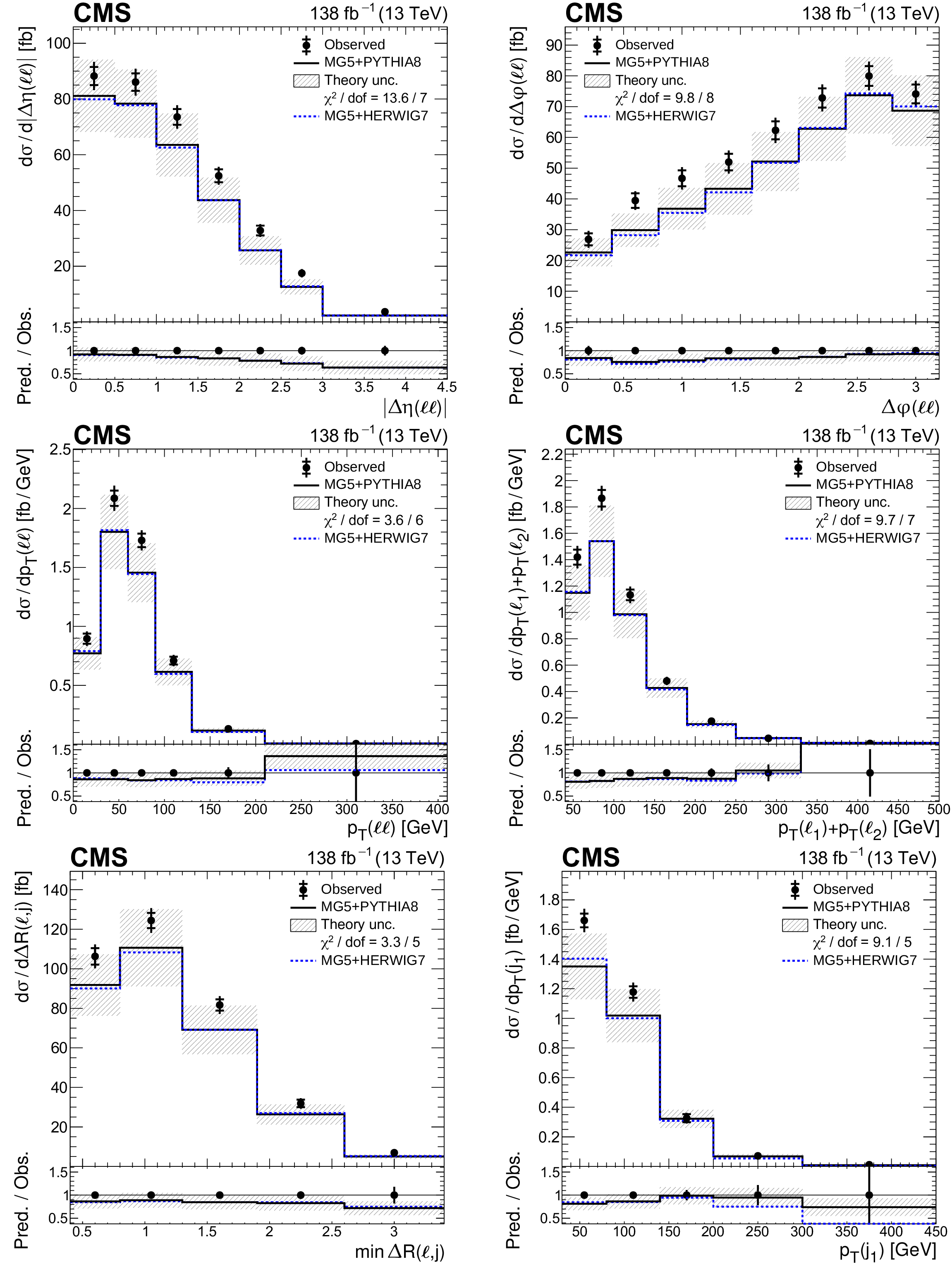
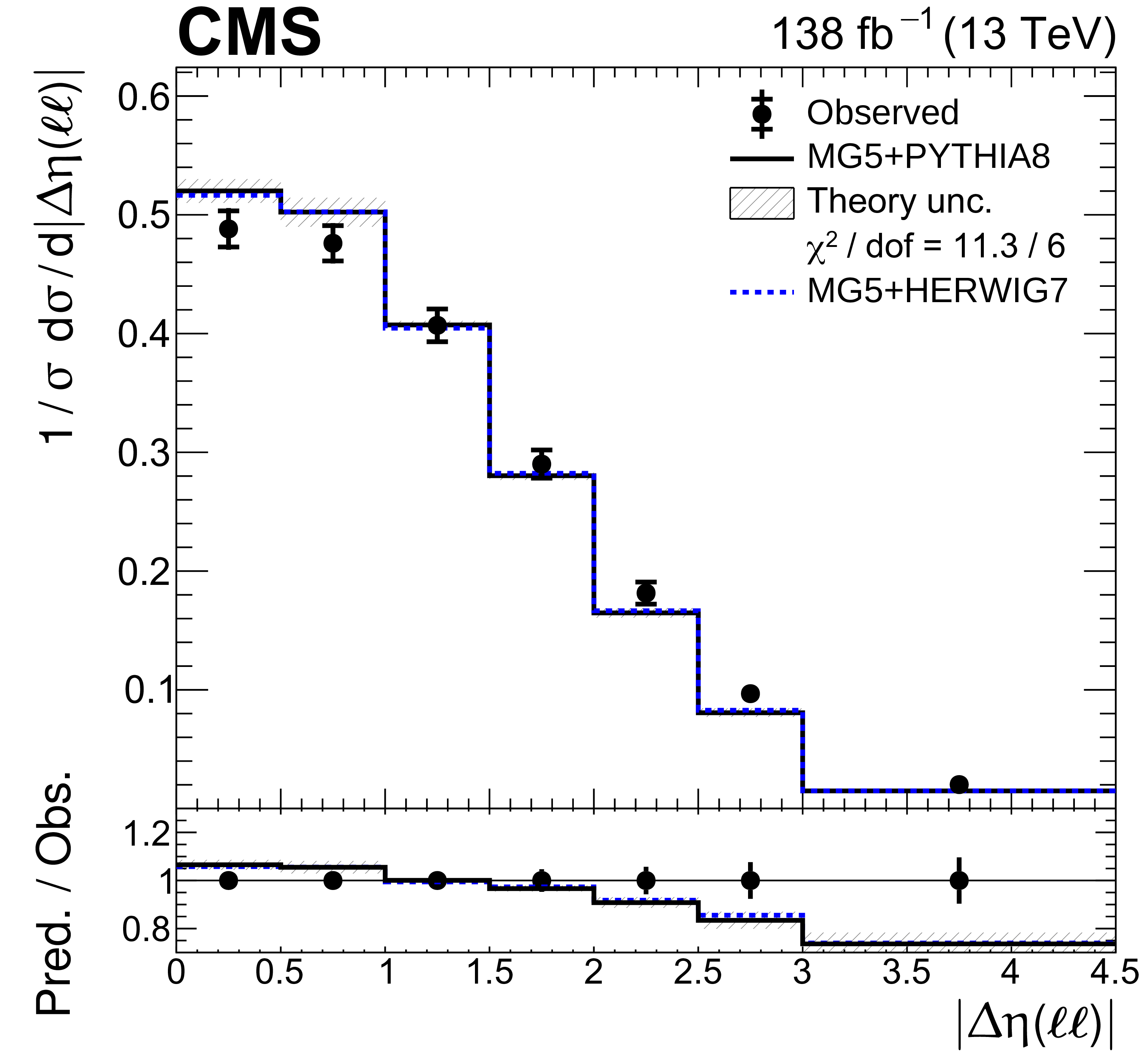
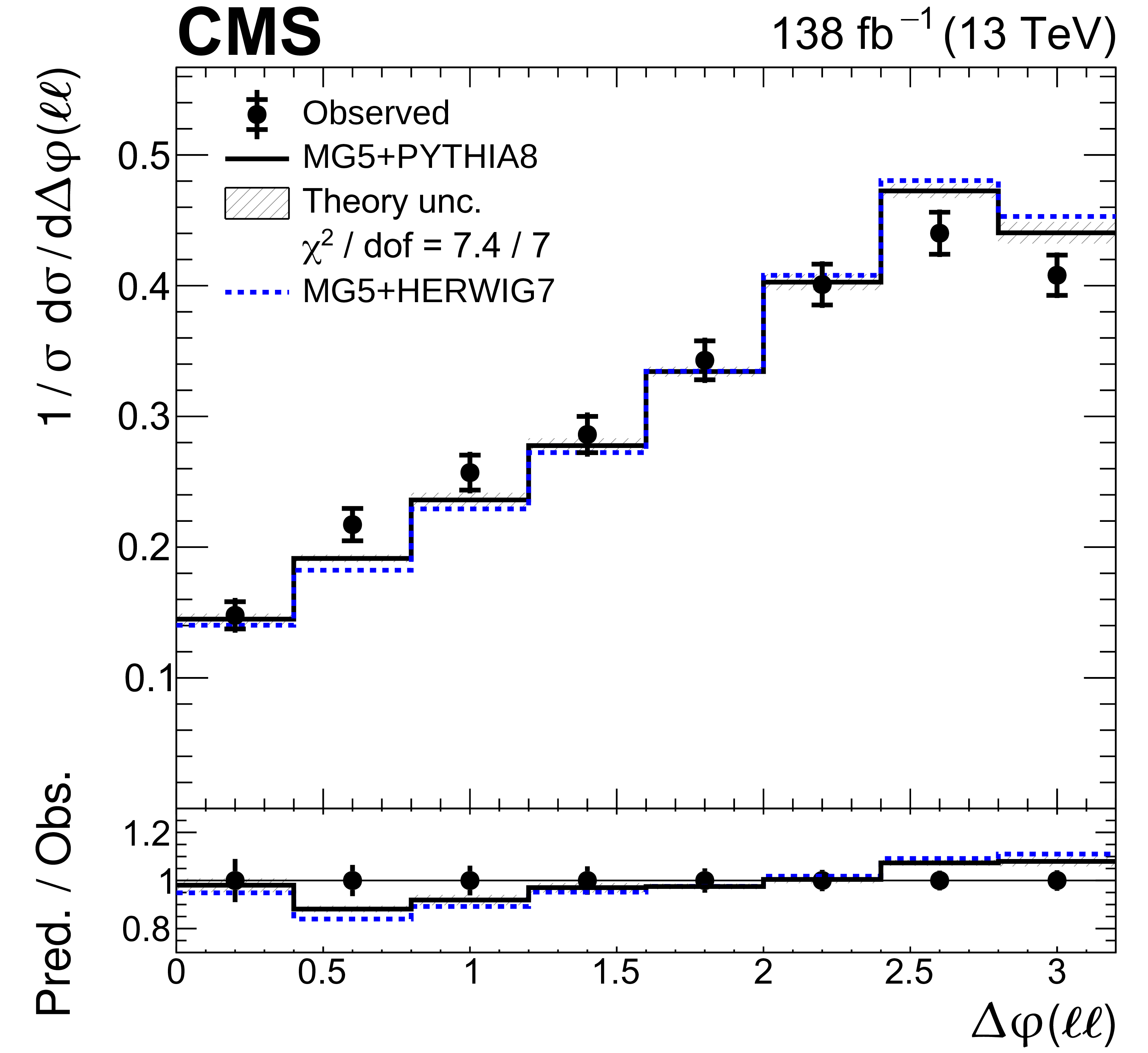
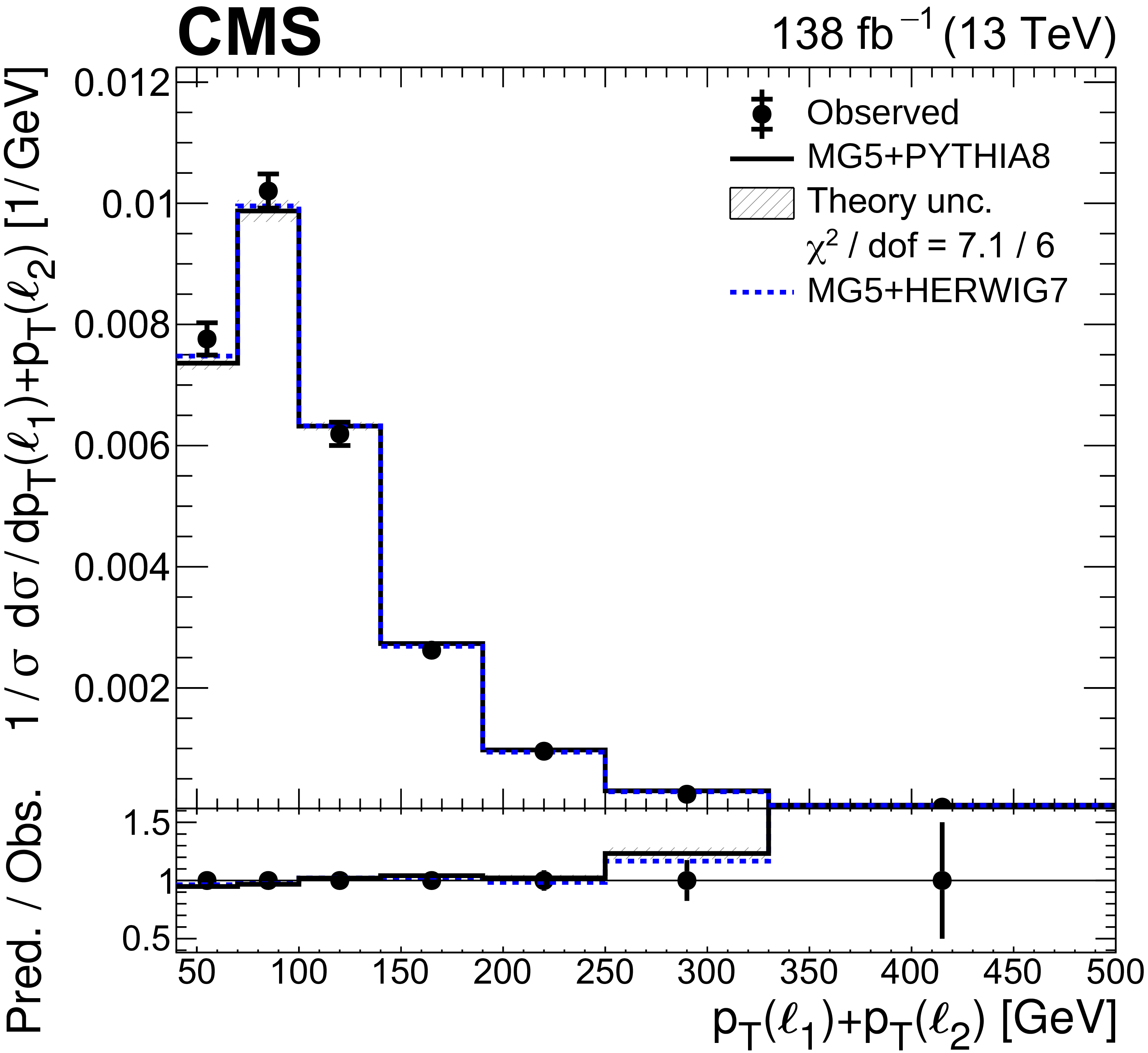
Figure 9:
Absolute differential ${{\mathrm{t} \mathrm{\bar{t}}} \gamma}$ production cross sections as functions of ${{| {\Delta \eta} (\ell \ell) |}}$ (upper left), ${{\Delta \varphi} (\ell \ell)}$ (upper right), ${{p_{\mathrm {T}}} (\ell \ell)}$ (middle left), ${{p_{\mathrm {T}}} (\ell _1)+ {p_{\mathrm {T}}} (\ell _2)}$ (middle right), ${\min {{\Delta R}} (\ell,\mathrm {j})}$ (lower left), and ${{p_{\mathrm {T}}} ({\mathrm {j}_1})}$ (lower right). Details can be found in the caption of Fig. 8. |

png pdf |
Figure 9-a:
Absolute differential ${{\mathrm{t} \mathrm{\bar{t}}} \gamma}$ production cross sections as functions of ${{| {\Delta \eta} (\ell \ell) |}}$. Details can be found in the caption of Fig. 8. |
png pdf |
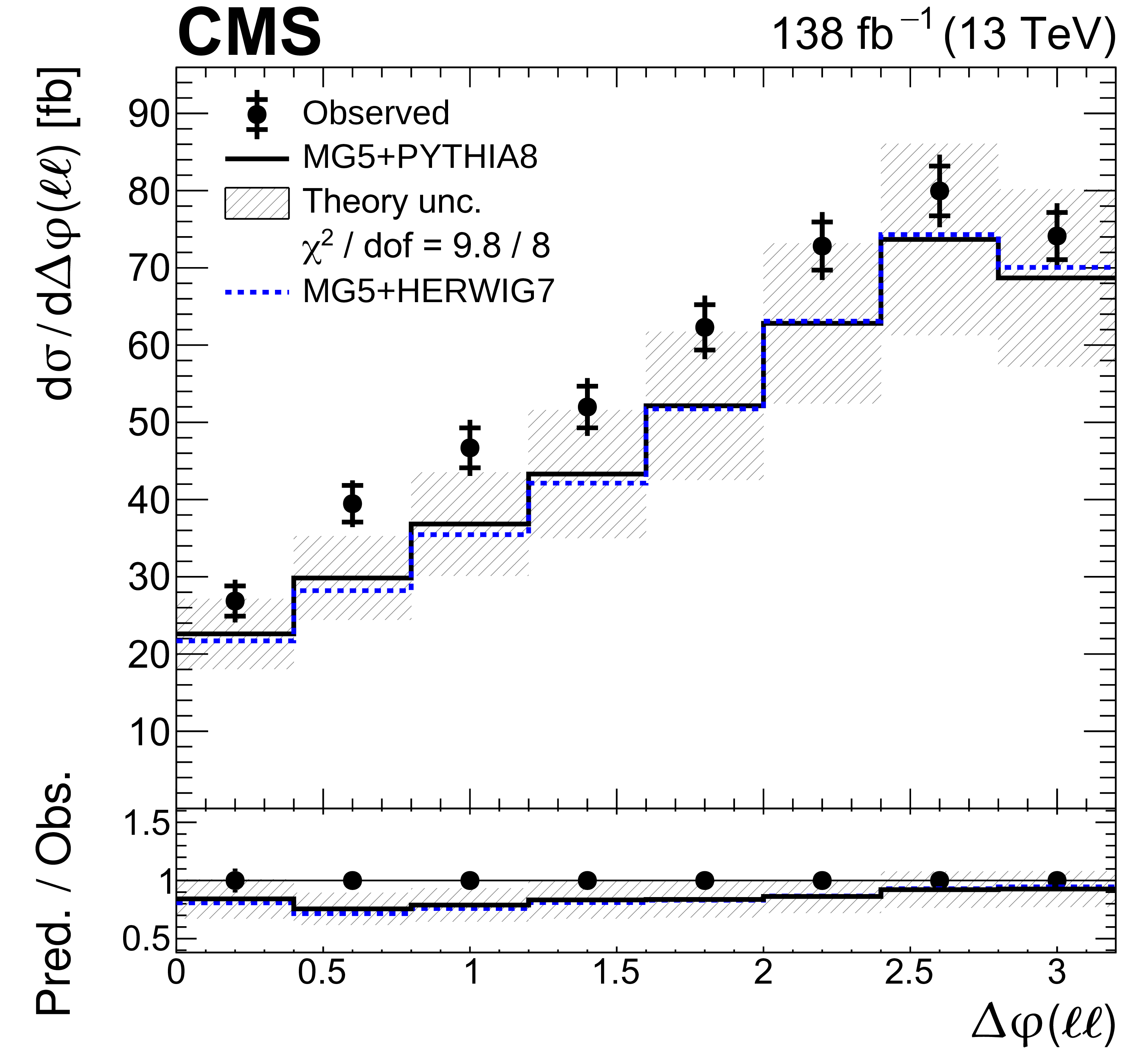
Figure 9-b:
Absolute differential ${{\mathrm{t} \mathrm{\bar{t}}} \gamma}$ production cross sections as functions of ${{\Delta \varphi} (\ell \ell)}$. ${{p_{\mathrm {T}}} (\ell \ell)}$. Details can be found in the caption of Fig. 8. |
png pdf |
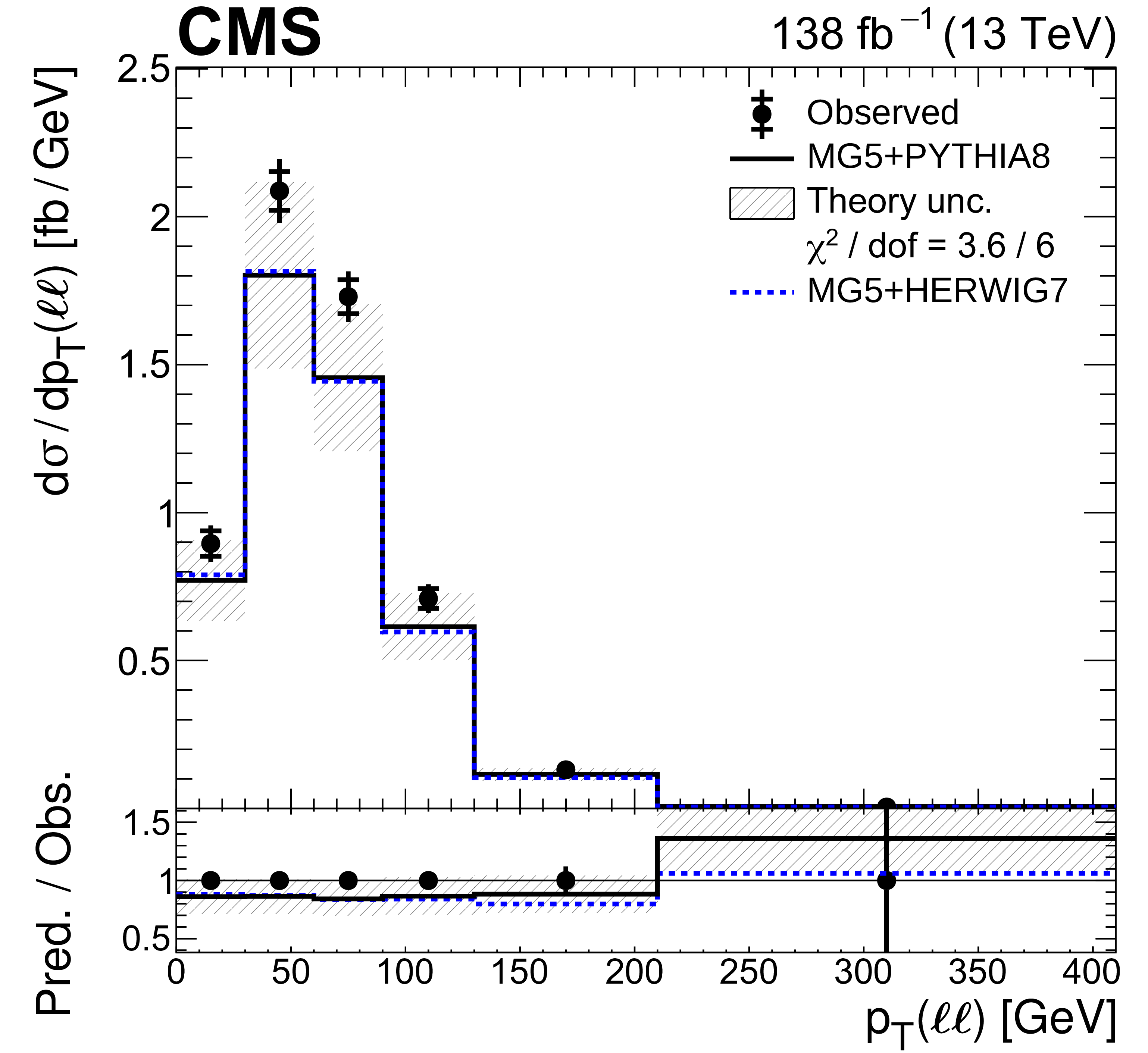
Figure 9-c:
Absolute differential ${{\mathrm{t} \mathrm{\bar{t}}} \gamma}$ production cross sections as functions of${{p_{\mathrm {T}}} (\ell \ell)}$. Details can be found in the caption of Fig. 8. |

png pdf |
Figure 9-d:
Absolute differential ${{\mathrm{t} \mathrm{\bar{t}}} \gamma}$ production cross sections as functions of ${{p_{\mathrm {T}}} (\ell _1)+ {p_{\mathrm {T}}} (\ell _2)}$. Details can be found in the caption of Fig. 8. |
png pdf |
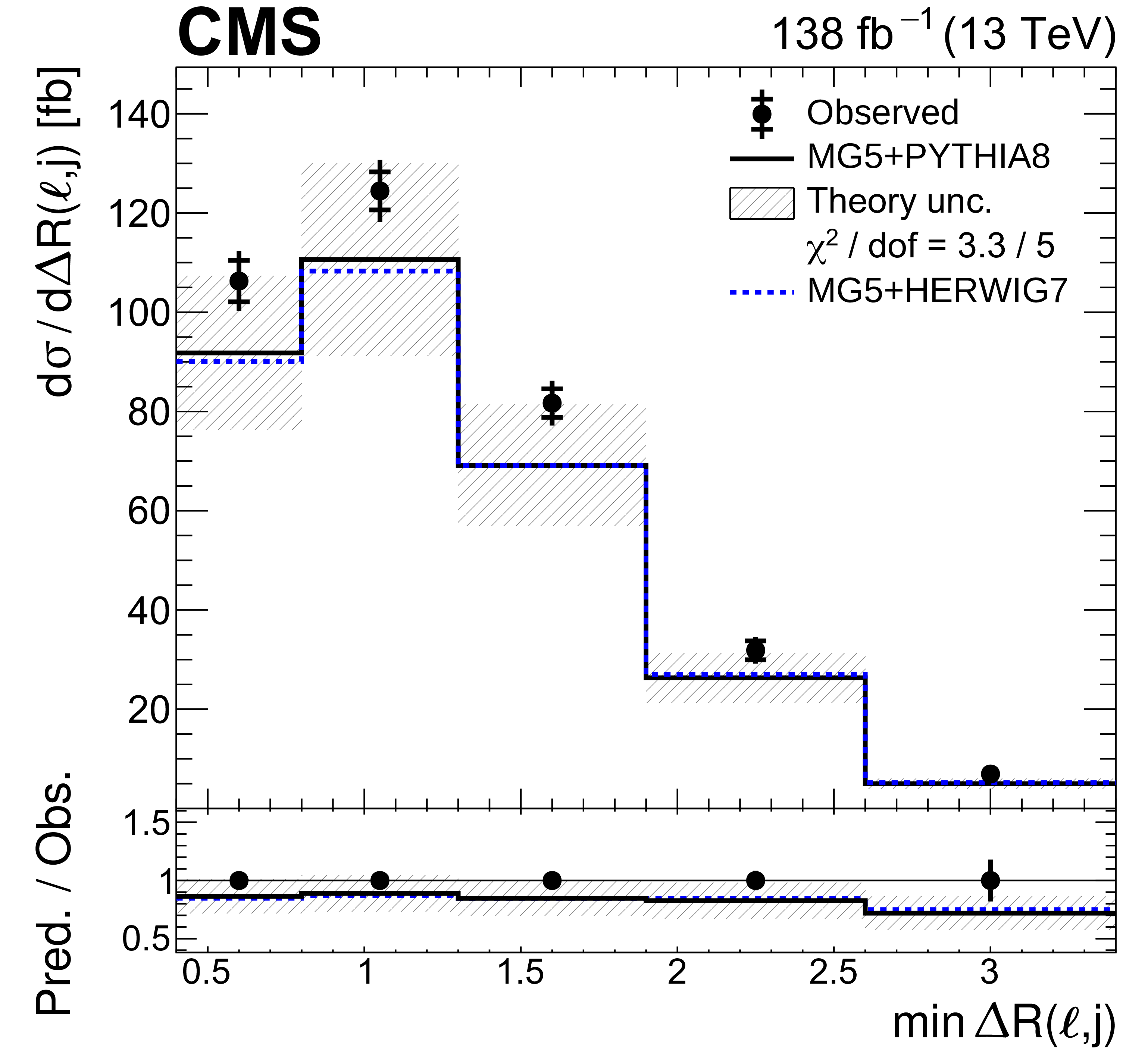
Figure 9-e:
Absolute differential ${{\mathrm{t} \mathrm{\bar{t}}} \gamma}$ production cross sections as functions of ${\min {{\Delta R}} (\ell,\mathrm {j})}$. Details can be found in the caption of Fig. 8. |

png pdf |
Figure 9-f:
Absolute differential ${{\mathrm{t} \mathrm{\bar{t}}} \gamma}$ production cross sections as functions of ${{p_{\mathrm {T}}} ({\mathrm {j}_1})}$. Details can be found in the caption of Fig. 8. |
png pdf |
Figure 10:
Normalized differential ${{\mathrm{t} \mathrm{\bar{t}}} \gamma}$ production cross sections as functions of ${{p_{\mathrm {T}}} (\gamma)}$ (upper left), ${{{| \eta |}} (\gamma)}$ (upper right), ${\min {{{\Delta R}} (\gamma,\ell)}}$ (middle left), ${{{\Delta R}} (\gamma,\ell _1)}$ (middle right), ${{{\Delta R}} (\gamma,\ell _2)}$ lower left), and ${\min {{\Delta R}} (\gamma,\mathrm{b})}$ (lower right). Details can be found in the caption of Fig. 8. |
png pdf |
Figure 10-a:
Normalized differential ${{\mathrm{t} \mathrm{\bar{t}}} \gamma}$ production cross sections as functions of ${{p_{\mathrm {T}}} (\gamma)}$. Details can be found in the caption of Fig. 8. |
png pdf |
Figure 10-b:
Normalized differential ${{\mathrm{t} \mathrm{\bar{t}}} \gamma}$ production cross sections as functions of ${{{| \eta |}} (\gamma)}$. Details can be found in the caption of Fig. 8. |
png pdf |
Figure 10-c:
Normalized differential ${{\mathrm{t} \mathrm{\bar{t}}} \gamma}$ production cross sections as functions of ${\min {{{\Delta R}} (\gamma,\ell)}}$. Details can be found in the caption of Fig. 8. |

png pdf |
Figure 10-d:
Normalized differential ${{\mathrm{t} \mathrm{\bar{t}}} \gamma}$ production cross sections as functions of ${{{\Delta R}} (\gamma,\ell _1)}$. Details can be found in the caption of Fig. 8. |
png pdf |
Figure 10-e:
Normalized differential ${{\mathrm{t} \mathrm{\bar{t}}} \gamma}$ production cross sections as functions of ${{{\Delta R}} (\gamma,\ell _2)}$. Details can be found in the caption of Fig. 8. |
png pdf |
Figure 10-f:
Normalized differential ${{\mathrm{t} \mathrm{\bar{t}}} \gamma}$ production cross sections as functions of ${\min {{\Delta R}} (\gamma,\mathrm{b})}$. Details can be found in the caption of Fig. 8. |

png pdf |
Figure 11:
Normalized differential ${{\mathrm{t} \mathrm{\bar{t}}} \gamma}$ production cross sections as functions of ${{| {\Delta \eta} (\ell \ell) |}}$ (upper left), ${{\Delta \varphi} (\ell \ell)}$ (upper right), ${{p_{\mathrm {T}}} (\ell \ell)}$ (middle left), ${{p_{\mathrm {T}}} (\ell _1)+ {p_{\mathrm {T}}} (\ell _2)}$ (middle right), ${\min {{\Delta R}} (\ell,\mathrm {j})}$ (lower left), and ${{p_{\mathrm {T}}} ({\mathrm {j}_1})}$ (lower right). Details can be found in the caption of Fig. 8. |
png pdf |
Figure 11-a:
Normalized differential ${{\mathrm{t} \mathrm{\bar{t}}} \gamma}$ production cross sections as functions of ${{| {\Delta \eta} (\ell \ell) |}}$. Details can be found in the caption of Fig. 8. |
png pdf |
Figure 11-b:
Normalized differential ${{\mathrm{t} \mathrm{\bar{t}}} \gamma}$ production cross sections as functions of ${{\Delta \varphi} (\ell \ell)}$. Details can be found in the caption of Fig. 8. |

png pdf |
Figure 11-c:
Normalized differential ${{\mathrm{t} \mathrm{\bar{t}}} \gamma}$ production cross sections as functions of ${{p_{\mathrm {T}}} (\ell \ell)}$. Details can be found in the caption of Fig. 8. |
png pdf |
Figure 11-d:
Normalized differential ${{\mathrm{t} \mathrm{\bar{t}}} \gamma}$ production cross sections as functions of ${{p_{\mathrm {T}}} (\ell _1)+ {p_{\mathrm {T}}} (\ell _2)}$. Details can be found in the caption of Fig. 8. |

png pdf |
Figure 11-e:
Normalized differential ${{\mathrm{t} \mathrm{\bar{t}}} \gamma}$ production cross sections as functions of ${\min {{\Delta R}} (\ell,\mathrm {j})}$. Details can be found in the caption of Fig. 8. |
png pdf |
Figure 11-f:
Normalized differential ${{\mathrm{t} \mathrm{\bar{t}}} \gamma}$ production cross sections as functions of ${{p_{\mathrm {T}}} ({\mathrm {j}_1})}$. Details can be found in the caption of Fig. 8. |
png pdf |
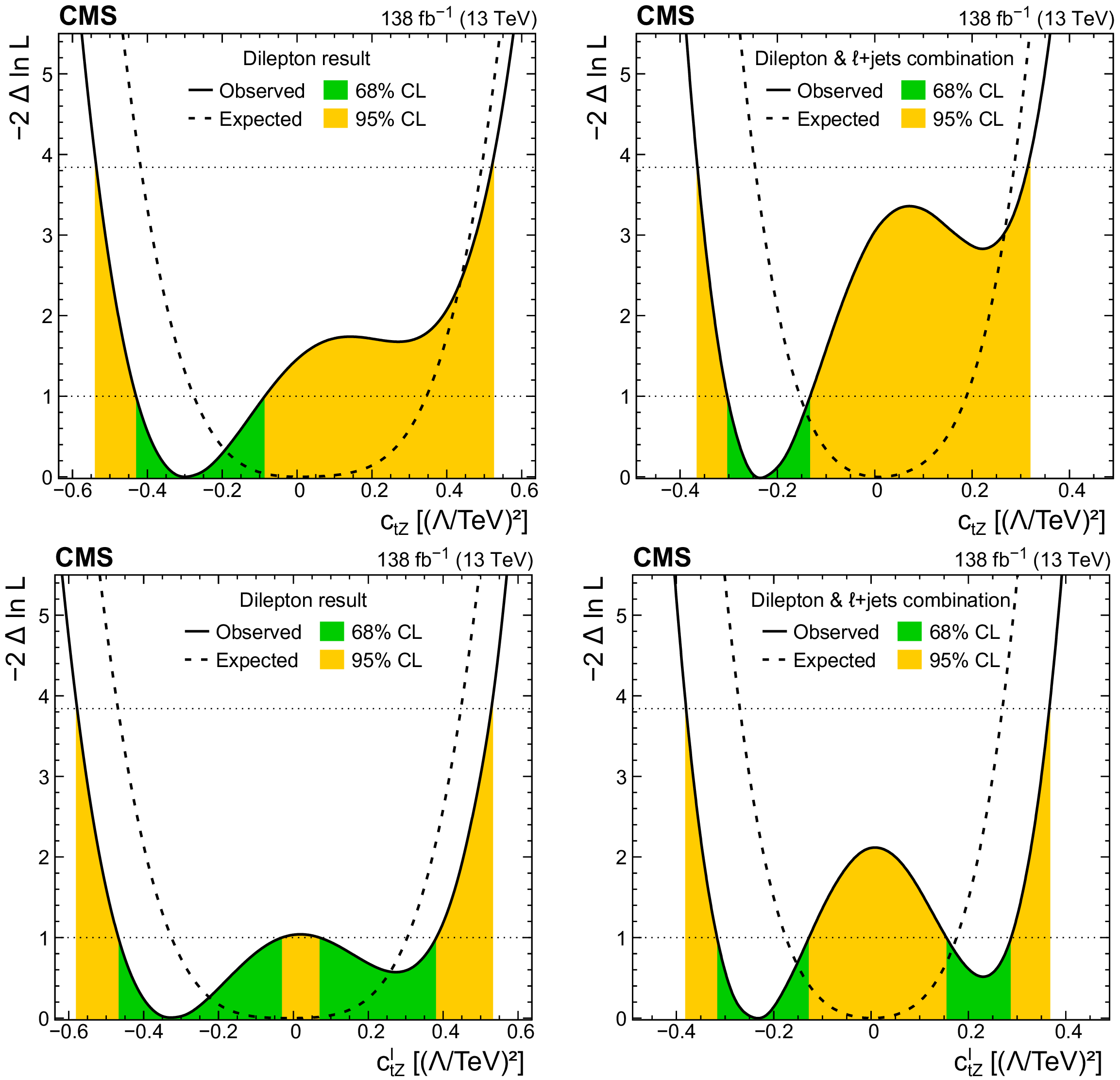
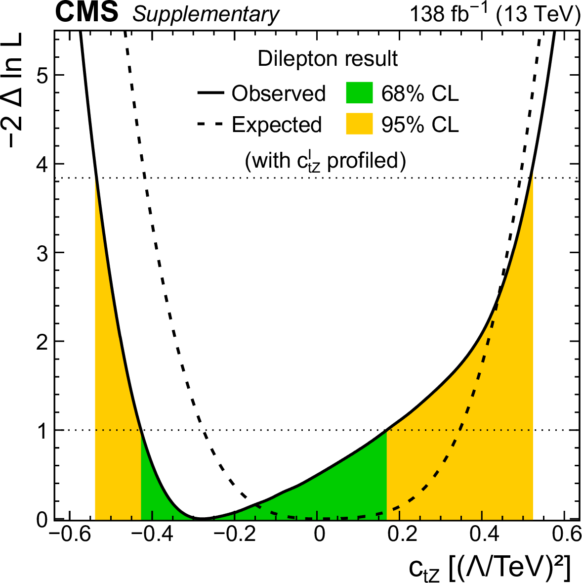
Figure 12:
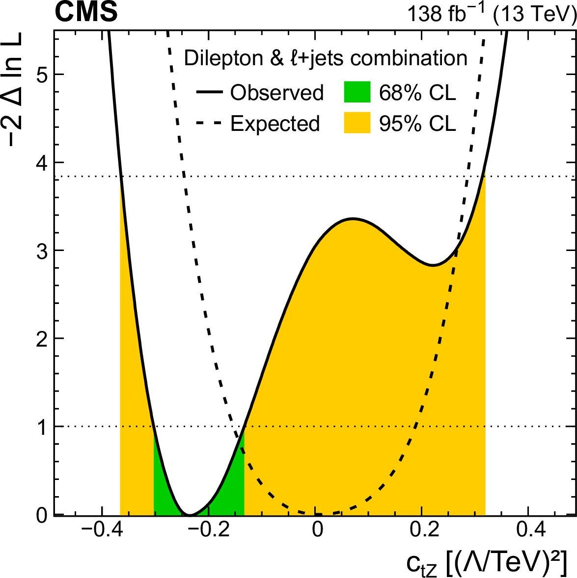
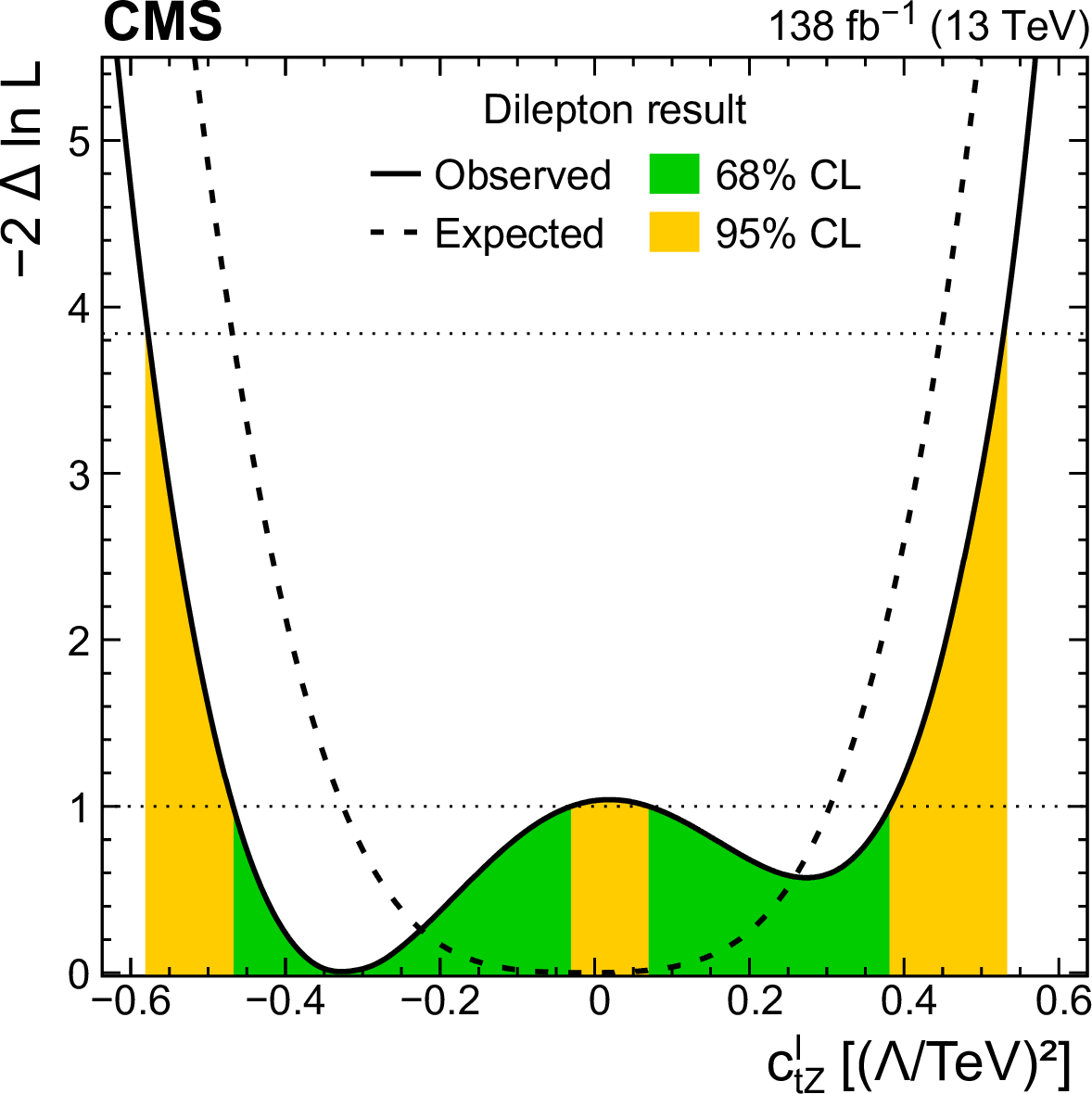
Distributions of the observed (solid line) and expected (dashed line) negative log-likelihood difference from the best fit value for the one-dimensional scans of the Wilson coefficients ${c_{\mathrm{t} \mathrm{Z}}}$ (upper) and ${c_{\mathrm{t} \mathrm{Z}}^{\mathrm {I}}}$ (lower), using the photon ${p_{\mathrm {T}}}$ distribution from this analysis (left) or the combination of this analysis with the $\ell$+jets analysis from Ref. [7] (right). In the scans, the other Wilson coefficient is set to zero. The green (orange) bands indicate the 68 (95)% CL limits on the Wilson coefficients. |

png pdf |
Figure 12-a:
Distributions of the observed (solid line) and expected (dashed line) negative log-likelihood difference from the best fit value for the one-dimensional scans of the Wilson coefficient ${c_{\mathrm{t} \mathrm{Z}}}$, using the photon ${p_{\mathrm {T}}}$ distribution from this analysis. In the scan, the other Wilson coefficient is set to zero. The green (orange) bands indicate the 68 (95)% CL limits on the Wilson coefficient. |
png pdf |
Figure 12-b:
Distributions of the observed (solid line) and expected (dashed line) negative log-likelihood difference from the best fit value for the one-dimensional scans of the Wilson coefficient ${c_{\mathrm{t} \mathrm{Z}}}$, using the photon ${p_{\mathrm {T}}}$ distribution from the combination of this analysis with the $\ell$+jets analysis from Ref. [7]. In the scan, the other Wilson coefficient is set to zero. The green (orange) bands indicate the 68 (95)% CL limits on the Wilson coefficient. |
png pdf |
Figure 12-c:
Distributions of the observed (solid line) and expected (dashed line) negative log-likelihood difference from the best fit value for the one-dimensional scans of the Wilson coefficient ${c_{\mathrm{t} \mathrm{Z}}^{\mathrm {I}}}$, using the photon ${p_{\mathrm {T}}}$ distribution from this analysis. In the scan, the other Wilson coefficient is set to zero. The green (orange) bands indicate the 68 (95)% CL limits on the Wilson coefficient. |

png pdf |
Figure 12-d:
Distributions of the observed (solid line) and expected (dashed line) negative log-likelihood difference from the best fit value for the one-dimensional scans of the Wilson coefficient ${c_{\mathrm{t} \mathrm{Z}}^{\mathrm {I}}}$, using the photon ${p_{\mathrm {T}}}$ distribution from the combination of this analysis with the $\ell$+jets analysis from Ref. [7]. In the scan, the other Wilson coefficient is set to zero. The green (orange) bands indicate the 68 (95)% CL limits on the Wilson coefficient. |

png pdf |
Figure 13:
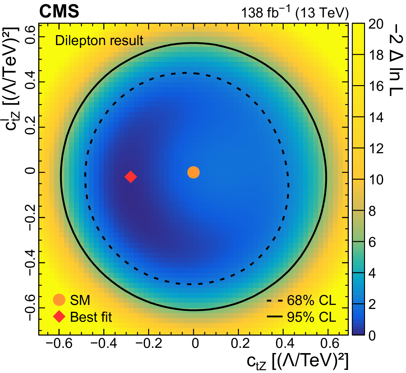
Result from the two-dimensional scan of the Wilson coefficients ${c_{\mathrm{t} \mathrm{Z}}}$ and ${c_{\mathrm{t} \mathrm{Z}}^{\mathrm {I}}}$ using the photon ${p_{\mathrm {T}}}$ distribution from this analysis (left) or the combination of this analysis with the $\ell$+jets analysis from Ref. [7] (right). The shading quantified by the colour scale on the right reflects the negative log-likelihood difference with respect to the best fit value that is indicated by the red diamond. The 68% (dashed curve) and 95% (solid curve) CL contours are shown for the observed result. The orange circle indicates the SM prediction. |
png pdf |
Figure 13-a:
Result from the two-dimensional scan of the Wilson coefficients ${c_{\mathrm{t} \mathrm{Z}}}$ and ${c_{\mathrm{t} \mathrm{Z}}^{\mathrm {I}}}$ using the photon ${p_{\mathrm {T}}}$ distribution from this analysis. The shading quantified by the colour scale on the right reflects the negative log-likelihood difference with respect to the best fit value that is indicated by the red diamond. The 68% (dashed curve) and 95% (solid curve) CL contours are shown for the observed result. The orange circle indicates the SM prediction. |

png pdf |
Figure 13-b:
Result from the two-dimensional scan of the Wilson coefficients ${c_{\mathrm{t} \mathrm{Z}}}$ and ${c_{\mathrm{t} \mathrm{Z}}^{\mathrm {I}}}$ using the photon ${p_{\mathrm {T}}}$ distribution from the combination of this analysis with the $\ell$+jets analysis from Ref. [7]. The shading quantified by the colour scale on the right reflects the negative log-likelihood difference with respect to the best fit value that is indicated by the red diamond. The 68% (dashed curve) and 95% (solid curve) CL contours are shown for the observed result. The orange circle indicates the SM prediction. |

png pdf |
Figure 14:
Comparison of observed 95% CL intervals for the Wilson coefficients ${c_{\mathrm{t} \mathrm{Z}}}$ (upper panel) and ${c_{\mathrm{t} \mathrm{Z}}^{\mathrm {I}}}$ (lower panel). For the CMS ${\mathrm{t} \mathrm{\bar{t}}} $Z [94], ${\mathrm{t} \mathrm{\bar{t}}} \gamma$ $\ell$+jets [7] and ${{\mathrm{t} \mathrm{\bar{t}}} \gamma}$ dilepton results, the limits are shown for the case where all other considered Wilson coefficients are fixed to zero. The dashed lines indicate the corresponding result of the ${\mathrm{t} \mathrm{\bar{t}}} \gamma$ $\ell$+jets and dilepton combination. For the CMS result based on ${\mathrm{t} \mathrm{\bar{t}}} $Z and tZq events [96], as well as from a global fit to the LHC, LEP, and Tevatron data [99], the limits where all other considered Wilson coefficients are fixed to zero are shown with solid lines, and the marginalized limits from the full fits are shown with dashed-and-dotted lines. |
| Tables | |
png pdf |
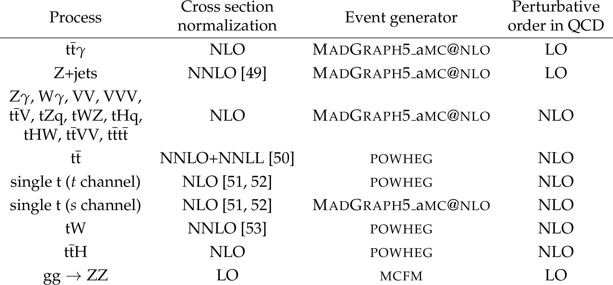
Table 1:
MC event generators used to simulate events for the signal and background processes. For each simulated process, the order of the cross section normalization calculation, the MC event generator used, and the perturbative order in QCD of the generator calculation are shown. The normalization and perturbative QCD orders are given as LO, NLO, next-to-NLO (NNLO), and including next-to-next-to-leading-logarithmic (NNLL) corrections. The symbol V refers to W and Z bosons. |
png pdf |
Table 2:
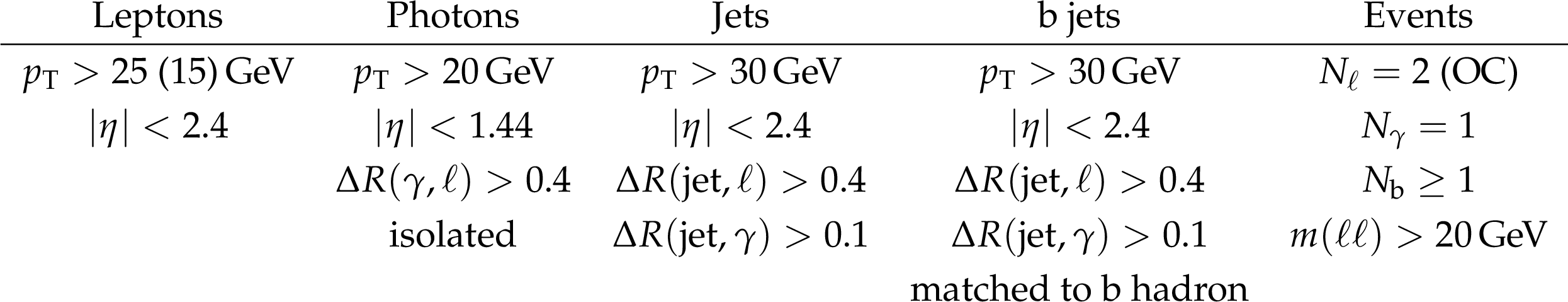
Summary of the requirements at the particle level on the various physics objects in the fiducial phase space definition. The two lepton ${p_{\mathrm {T}}}$ thresholds are applied to the highest and second-highest ${p_{\mathrm {T}}}$ lepton, respectively. The "isolated'' definition for the photon requires no stable particle with $ {p_{\mathrm {T}}} > $ 5 GeV except neutrinos within a cone of $ {{\Delta R}} =$ 0.1. The parameters ${N_{\ell}}$, ${N_{\gamma}}$, and ${N_{\mathrm{b}}}$ represent the numbers of leptons, photons, and b jets, respectively, in the event. |

png pdf |
Table 3:
Summary of the systematic uncertainty sources in the ${{\mathrm{t} \mathrm{\bar{t}}} \gamma}$ cross section measurements. The first column lists the source of the uncertainty. The second column indicates the treatment of correlations between the uncertainties in the three data-taking years, where ~ means fully correlated, ${\sim}$ means partially correlated, and ${\times}$ means uncorrelated. For each systematic source, the "prefit'' uncertainty is estimated from a cut-and-count analysis of the expected and observed event yields separately in bins of ${{p_{\mathrm {T}}} (\gamma)}$ and for the three data-taking years using the input variations; the typical range across the three years is shown in the third column and can be compared between the different uncertainty sources. The last column gives the impact of each uncertainty source on the measured inclusive ${{\mathrm{t} \mathrm{\bar{t}}} \gamma}$ cross section after the fit to the data ("postfit''). The last two rows give the statistical and total uncertainty in the measured cross section. |

png pdf |
Table 4:
Definition of the observables used in the differential cross section measurement. |

png pdf |
Table 5:
Summary of the one-dimensional 68 and 95% CL intervals obtained for the Wilson coefficients ${c_{\mathrm{t} \mathrm{Z}}}$ and ${c_{\mathrm{t} \mathrm{Z}}^{\mathrm {I}}}$ using the photon ${p_{\mathrm {T}}}$ distribution from this analysis or the combination of this analysis with the $\ell$+jets analysis from Ref. [7]. The profiled results correspond to the fits where the other Wilson coefficient is left free in the fit, otherwise it is set to zero. |
| Summary |
|
A measurement of the inclusive and differential cross sections for top quark pair production in association with a photon (${\mathrm{t\bar{t}}\gamma}$) has been presented, using 138 fb$^{-1}$ of proton-proton (pp) collision data at $\sqrt{s} =$ 13 TeV recorded with the CMS detector at the LHC. The analysis is performed in a fiducial phase space defined at the particle level by the requirement of exactly one isolated photon, exactly two oppositely charged leptons, and at least one jet coming from the hadronization of a bottom quark, including the ${\mathrm{e^{\pm}}\mu^{\mp}}$, ${\mathrm{e^{+}}\mathrm{e^{-}}}$, and $\mu^{+}\mu^{-}$ channels of the $\mathrm{t\bar{t}}$ decay. The inclusive cross section is extracted with a profile likelihood fit to the transverse momentum distribution of the reconstructed photon, and is measured to be ${\sigma_\text{fid}(\mathrm{ pp \to t\bar{t}\gamma })} =$ 173.5 $\pm$ 2.5 (stat) $\pm$ 6.3 (syst) fb, in agreement with the standard model (SM) prediction of ${\sigma_\text{SM}(\mathrm{ pp \to t\bar{t}\gamma })} = $ 153 $\pm$ 27 fb. Differential cross sections are measured as functions of various kinematic properties of the photon, leptons, and jets, and unfolded to the particle level. The comparison to SM predictions is performed using different parton shower algorithms. No significant deviations from the SM predictions are found. The measurements are also interpreted in terms of the SM effective field theory. Constraints are derived on the Wilson coefficients ${c_{\mathrm{t}\mathrm{Z}}}$ and ${c_{\mathrm{t}\mathrm{Z}}^{\mathrm{I}}}$ describing the modifications of the$\mathrm{t\bar{t}}$Z and ${\mathrm{t\bar{t}}\gamma}$ interaction vertices, from these results alone and in combination with another CMS measurement of ${\mathrm{t\bar{t}}\gamma}$ production using the lepton+jets final state and the same data set. From the combined interpretation, the best experimental limits on these Wilson coefficients to date are derived. |
| Additional Figures | |
png pdf |
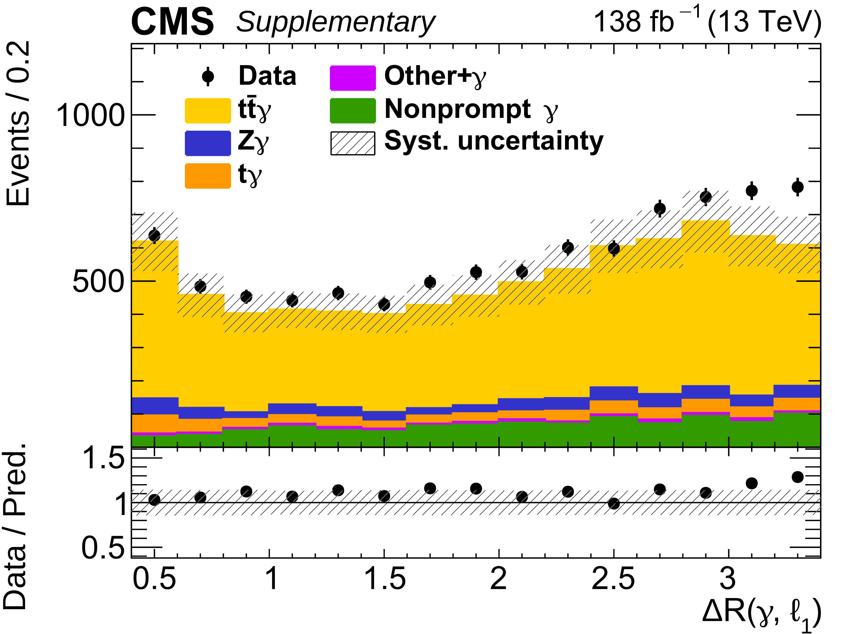
Additional Figure 1:
The observed (points) and predicted (shaded histograms) signal and background yields as functions of the angular separation between the photon and the leading lepton after applying the signal selection. The distribution is shown for the three lepton flavour channels combined, with all relevant corrections applied. The predictions are normalized to the expected yields, without taking the results of the fit to the data into account. The vertical bars on the points show the statistical uncertainties in the data, and the hatched bands the systematic uncertainty in the predictions. The lower panel shows the ratio of the event yields in data to the overall sum of the predictions. |

png pdf |
Additional Figure 2:
The observed (points) and predicted (shaded histograms) signal and background yields as functions of the angular separation between the photon and the subleading lepton after applying the signal selection. The distribution is shown for the three lepton flavour channels combined, with all relevant corrections applied. The predictions are normalized to the expected yields, without taking the results of the fit to the data into account. The vertical bars on the points show the statistical uncertainties in the data, and the hatched bands the systematic uncertainty in the predictions. The lower panel shows the ratio of the event yields in data to the overall sum of the predictions. |
png pdf |
Additional Figure 3:
The observed (points) and predicted (shaded histograms) signal and background yields as functions of the angular separation between the photon and the closest b jet after applying the signal selection. The distribution is shown for the three lepton flavour channels combined, with all relevant corrections applied. The predictions are normalized to the expected yields, without taking the results of the fit to the data into account. The vertical bars on the points show the statistical uncertainties in the data, and the hatched bands the systematic uncertainty in the predictions. The lower panel shows the ratio of the event yields in data to the overall sum of the predictions. |
png pdf |
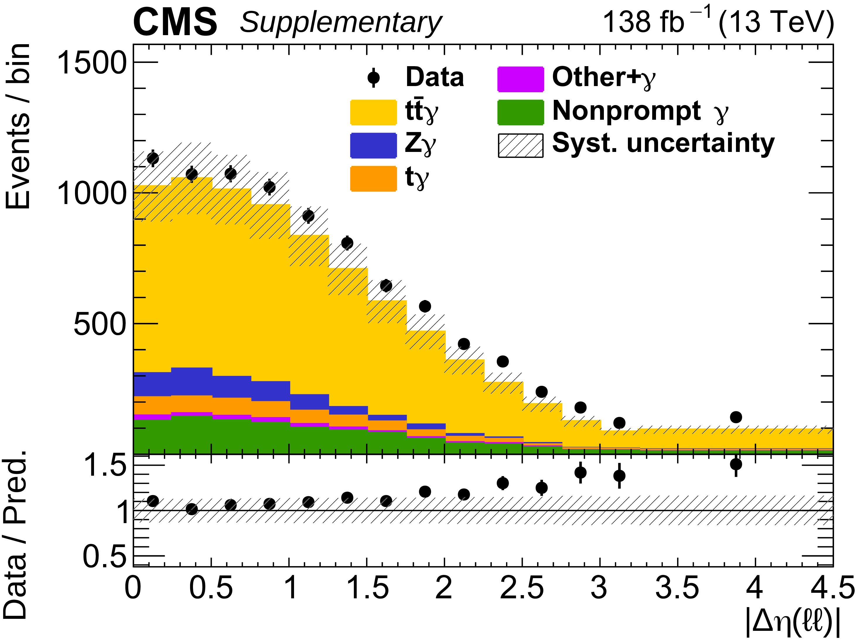
Additional Figure 4:
The observed (points) and predicted (shaded histograms) signal and background yields as functions of the pseudorapidity difference between the two leptons after applying the signal selection. The distribution is shown for the three lepton flavour channels combined, with all relevant corrections applied. The predictions are normalized to the expected yields, without taking the results of the fit to the data into account. The vertical bars on the points show the statistical uncertainties in the data, and the hatched bands the systematic uncertainty in the predictions. The lower panel shows the ratio of the event yields in data to the overall sum of the predictions. |
png pdf |
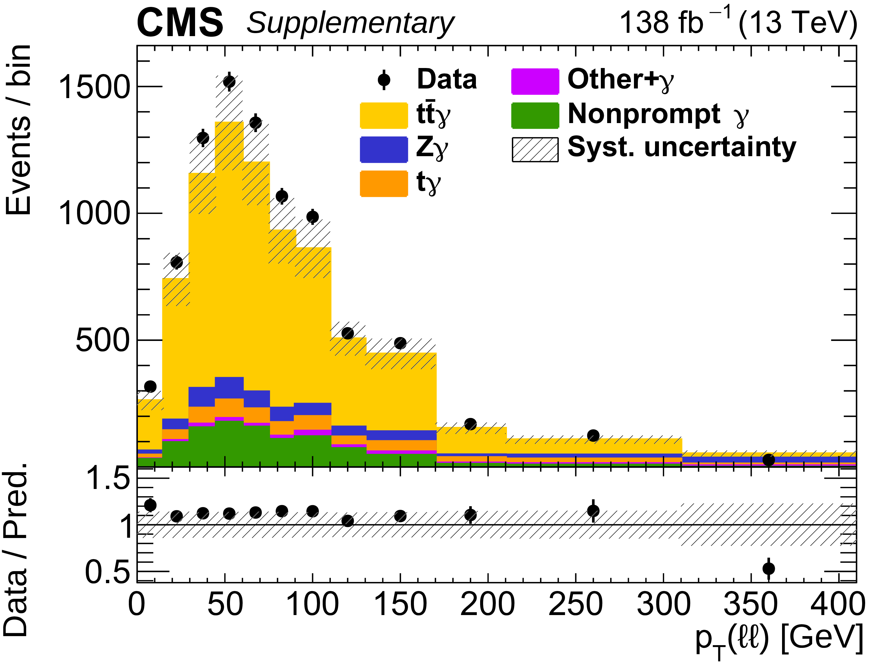
Additional Figure 5:
The observed (points) and predicted (shaded histograms) signal and background yields as functions of the ${p_{\mathrm {T}}}$ of the dilepton system after applying the signal selection. The distribution is shown for the three lepton flavour channels combined, with all relevant corrections applied. The predictions are normalized to the expected yields, without taking the results of the fit to the data into account. The vertical bars on the points show the statistical uncertainties in the data, and the hatched bands the systematic uncertainty in the predictions. The lower panel shows the ratio of the event yields in data to the overall sum of the predictions. |
png pdf |
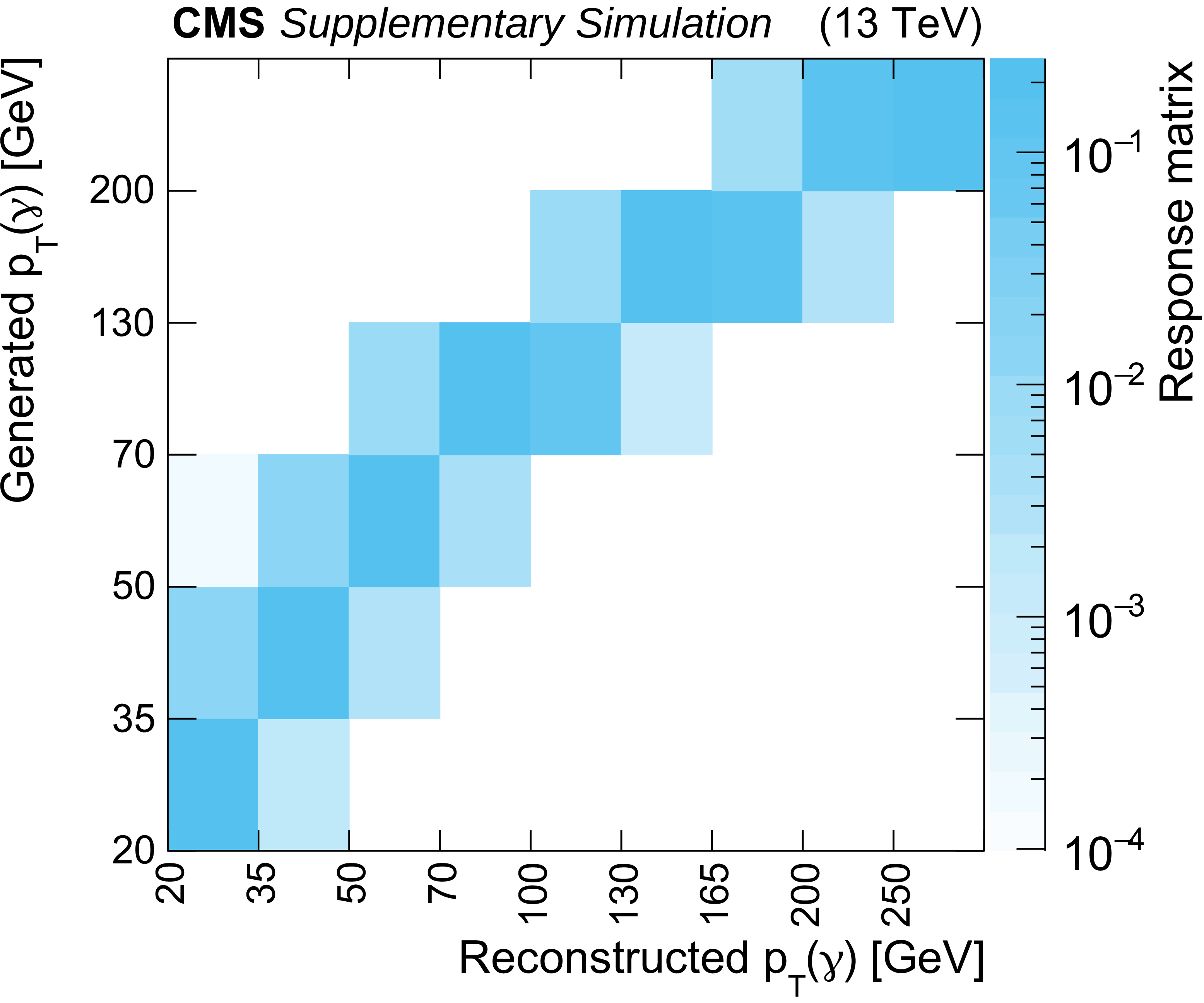
Additional Figure 6:
Response matrix describing the probability for a ${\mathrm{t} {}\mathrm{\bar{t}}} \gamma $ event generated in the fiducial phase space with a certain value of the photon ${p_{\mathrm {T}}}$ to be selected with a reconstructed photon a certain ${p_{\mathrm {T}}}$. |

png pdf |
Additional Figure 7:
Response matrix describing the probability for a ${\mathrm{t} {}\mathrm{\bar{t}}} \gamma $ event generated in the fiducial phase space with a certain value of the jet ${p_{\mathrm {T}}}$ to be selected with a reconstructed jet of a certain ${p_{\mathrm {T}}}$. |

png pdf |
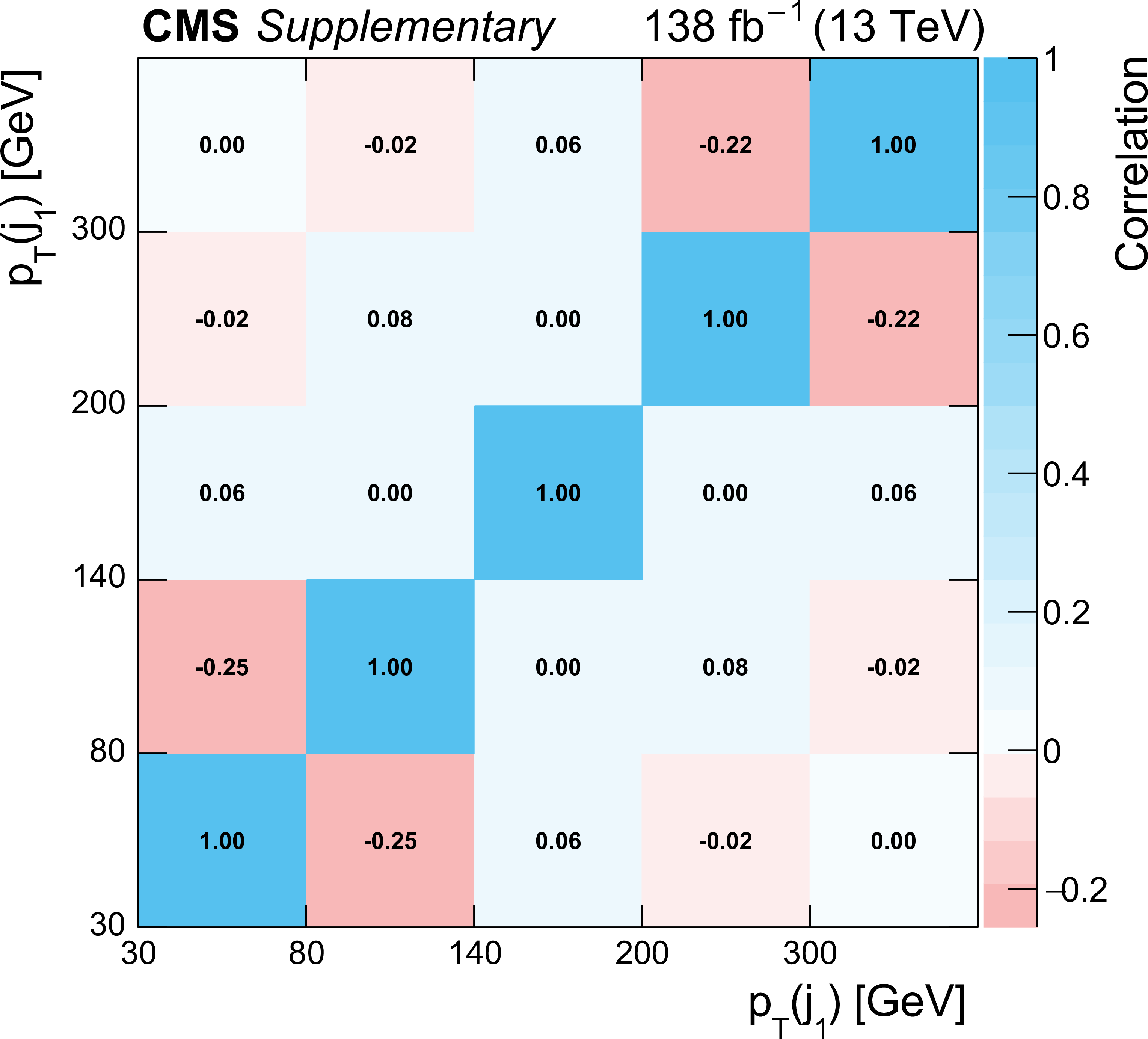
Additional Figure 8:
Systematic correlation between the bins of the measured absolute differential cross section as a function of $ {p_{\mathrm {T}}} (\gamma)$. |
png pdf |
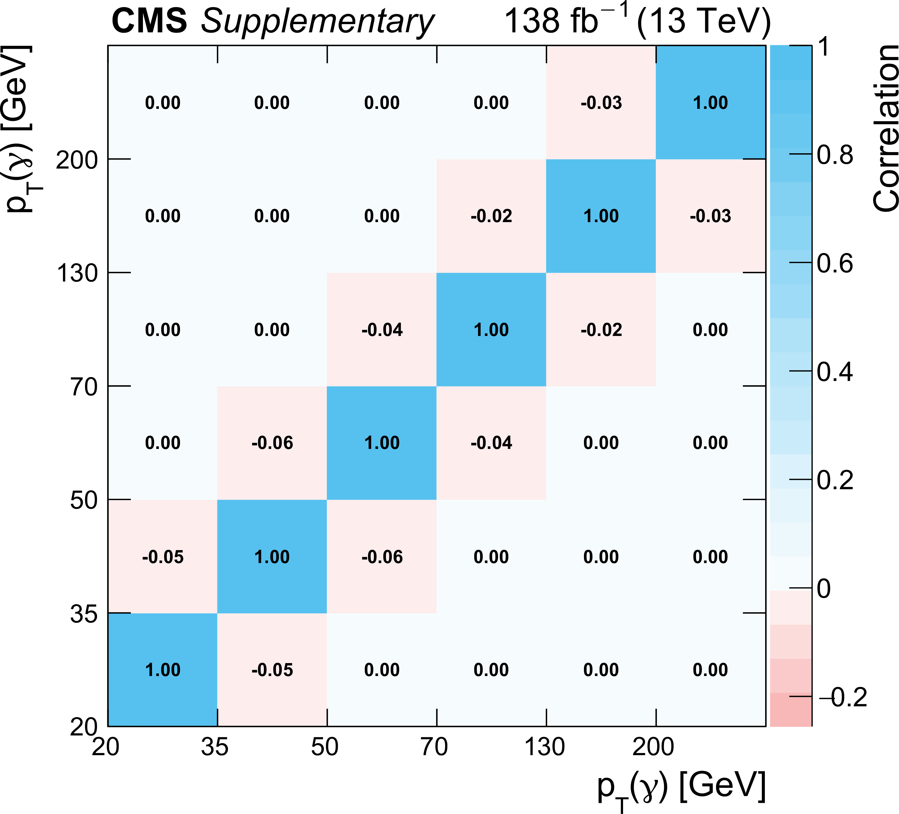
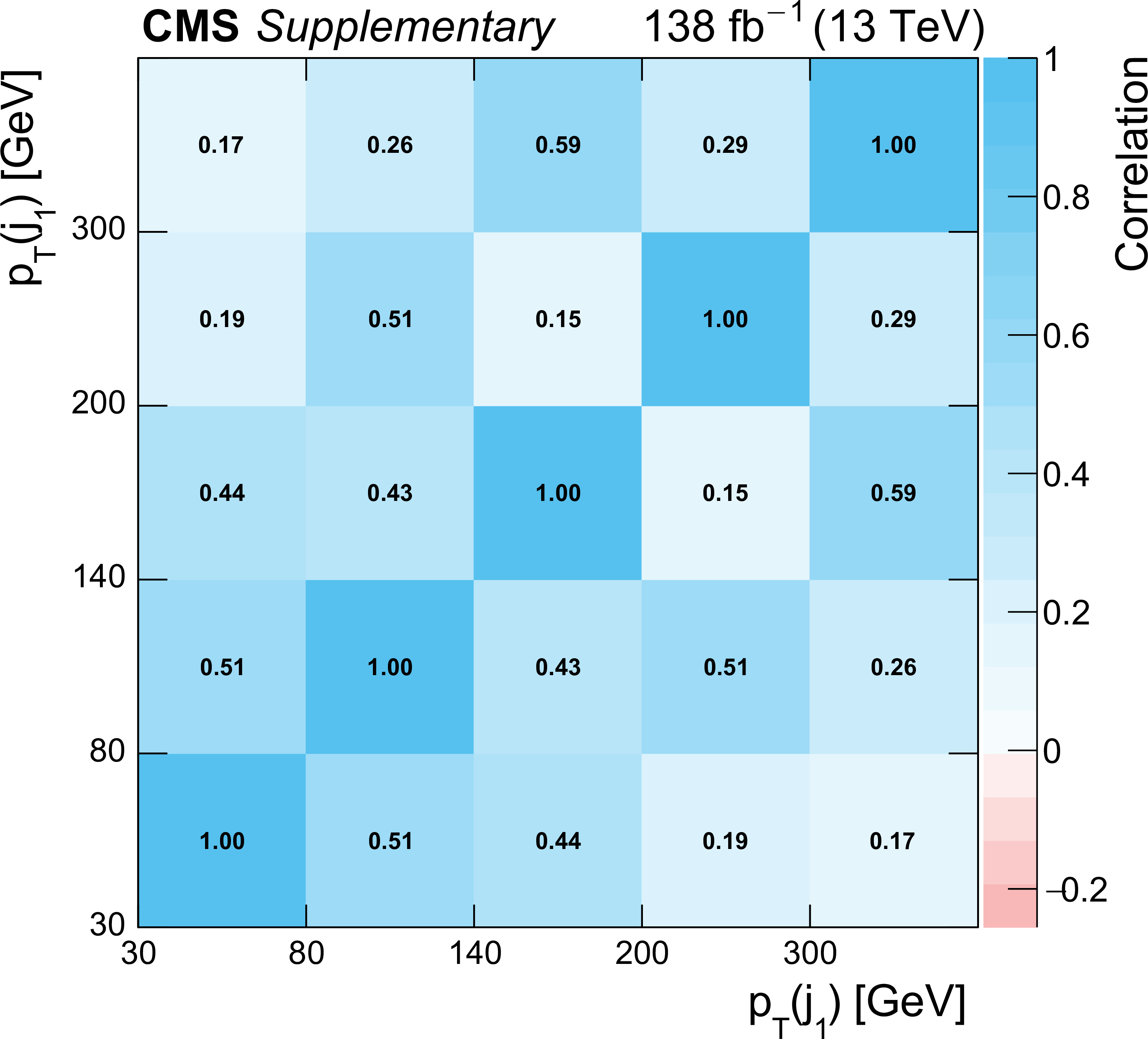
Additional Figure 9:
Statistical correlation between the bins of the measured absolute differential cross section as a function of $ {p_{\mathrm {T}}} (\gamma)$. |
png pdf |
Additional Figure 10:
Systematic correlation between the bins of the measured absolute differential cross section as a function of $ {| \eta |}(\gamma)$. |

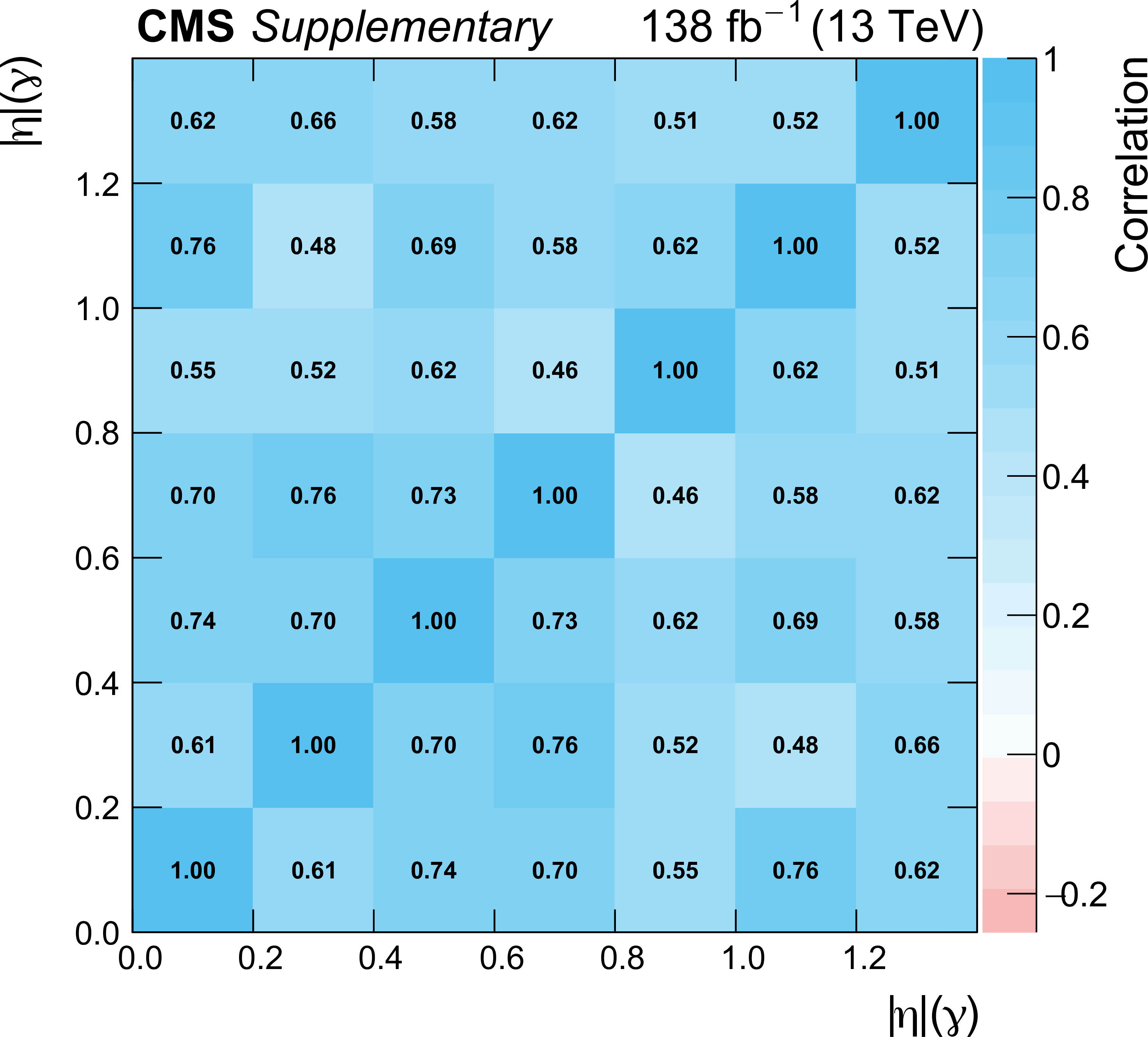
png pdf |
Additional Figure 11:
Statistical correlation between the bins of the measured absolute differential cross section as a function of $ {| \eta |}(\gamma)$. |

png pdf |
Additional Figure 12:
Systematic correlation between the bins of the measured absolute differential cross section as a function of $\min {\Delta R}(\gamma,\ell)$. |

png pdf |
Additional Figure 13:
Statistical correlation between the bins of the measured absolute differential cross section as a function of $\min {\Delta R}(\gamma,\ell)$. |
png pdf |
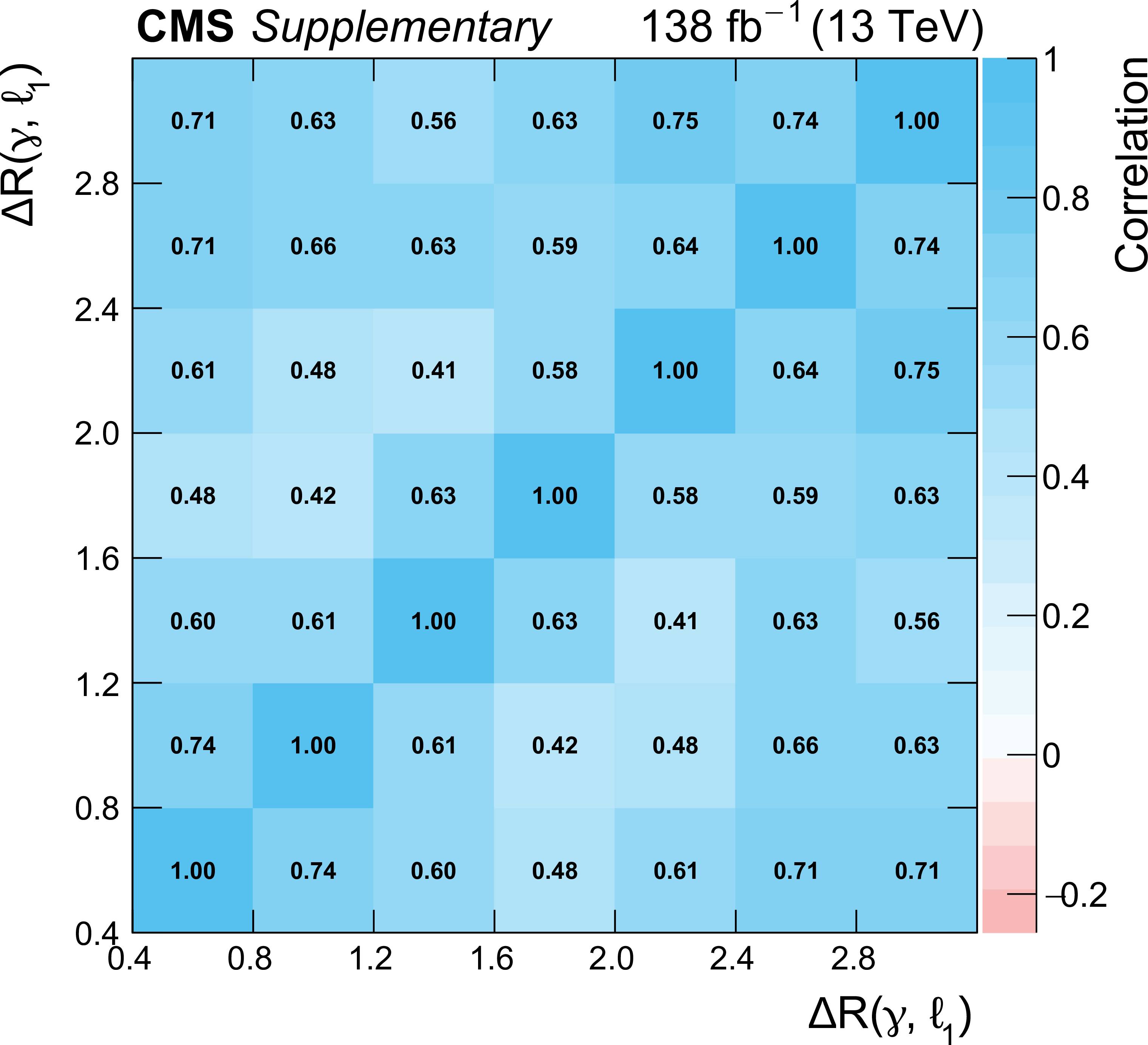
Additional Figure 14:
Systematic correlation between the bins of the measured absolute differential cross section as a function of $ {\Delta R}(\gamma,\ell _1)$. |

png pdf |
Additional Figure 15:
Statistical correlation between the bins of the measured absolute differential cross section as a function of $ {\Delta R}(\gamma,\ell _1)$. |

png pdf |
Additional Figure 16:
Systematic correlation between the bins of the measured absolute differential cross section as a function of $ {\Delta R}(\gamma,\ell _2)$. |

png pdf |
Additional Figure 17:
Statistical correlation between the bins of the measured absolute differential cross section as a function of $ {\Delta R}(\gamma,\ell _2)$. |
png pdf |
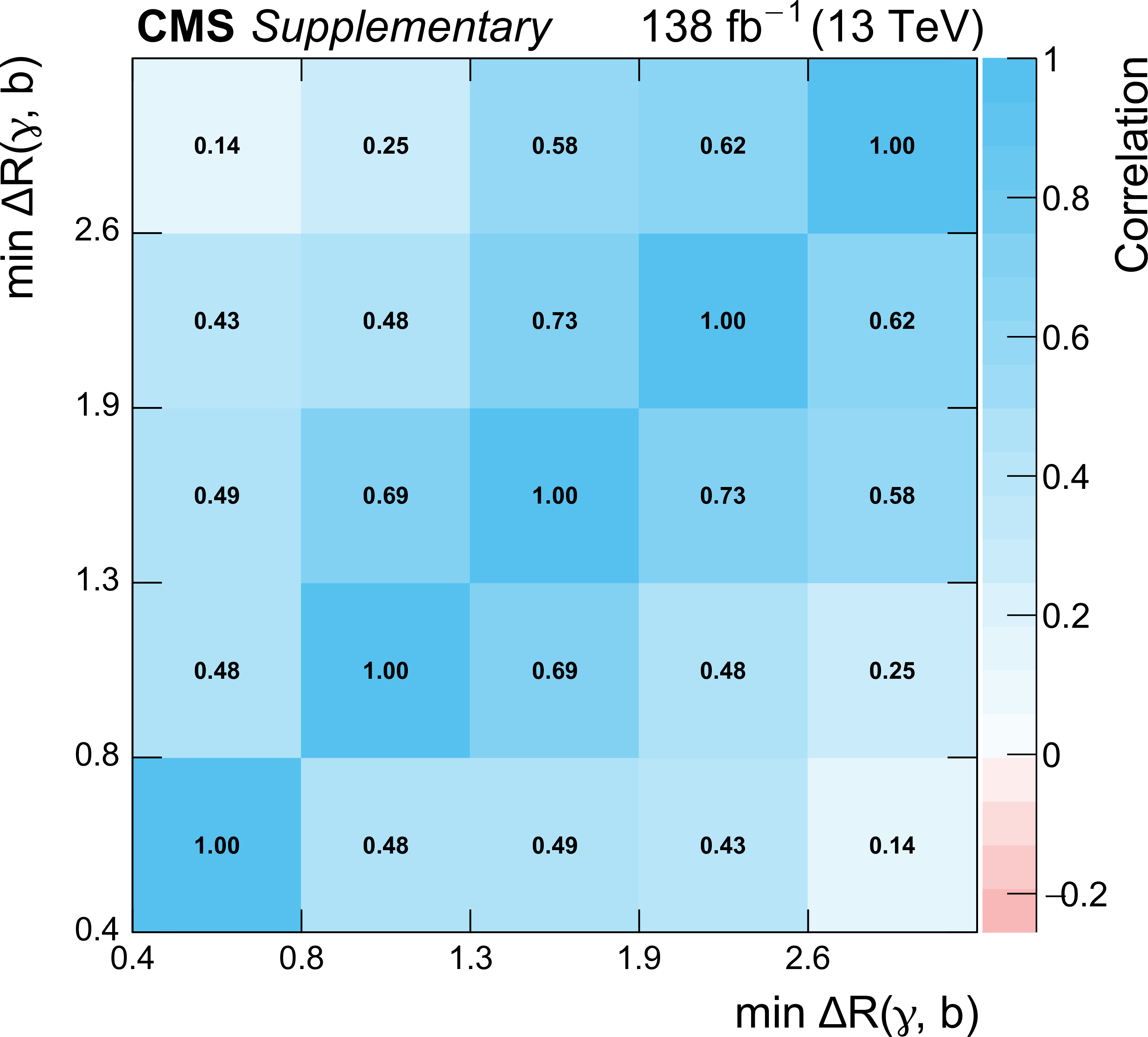
Additional Figure 18:
Systematic correlation between the bins of the measured absolute differential cross section as a function of $\min {\Delta R}(\gamma,\mathrm{b})$. |

png pdf |
Additional Figure 19:
Statistical correlation between the bins of the measured absolute differential cross section as a function of $\min {\Delta R}(\gamma,\mathrm{b})$. |

png pdf |
Additional Figure 20:
Systematic correlation between the bins of the measured absolute differential cross section as a function of $ {| \Delta \eta (\ell \ell) |}$. |
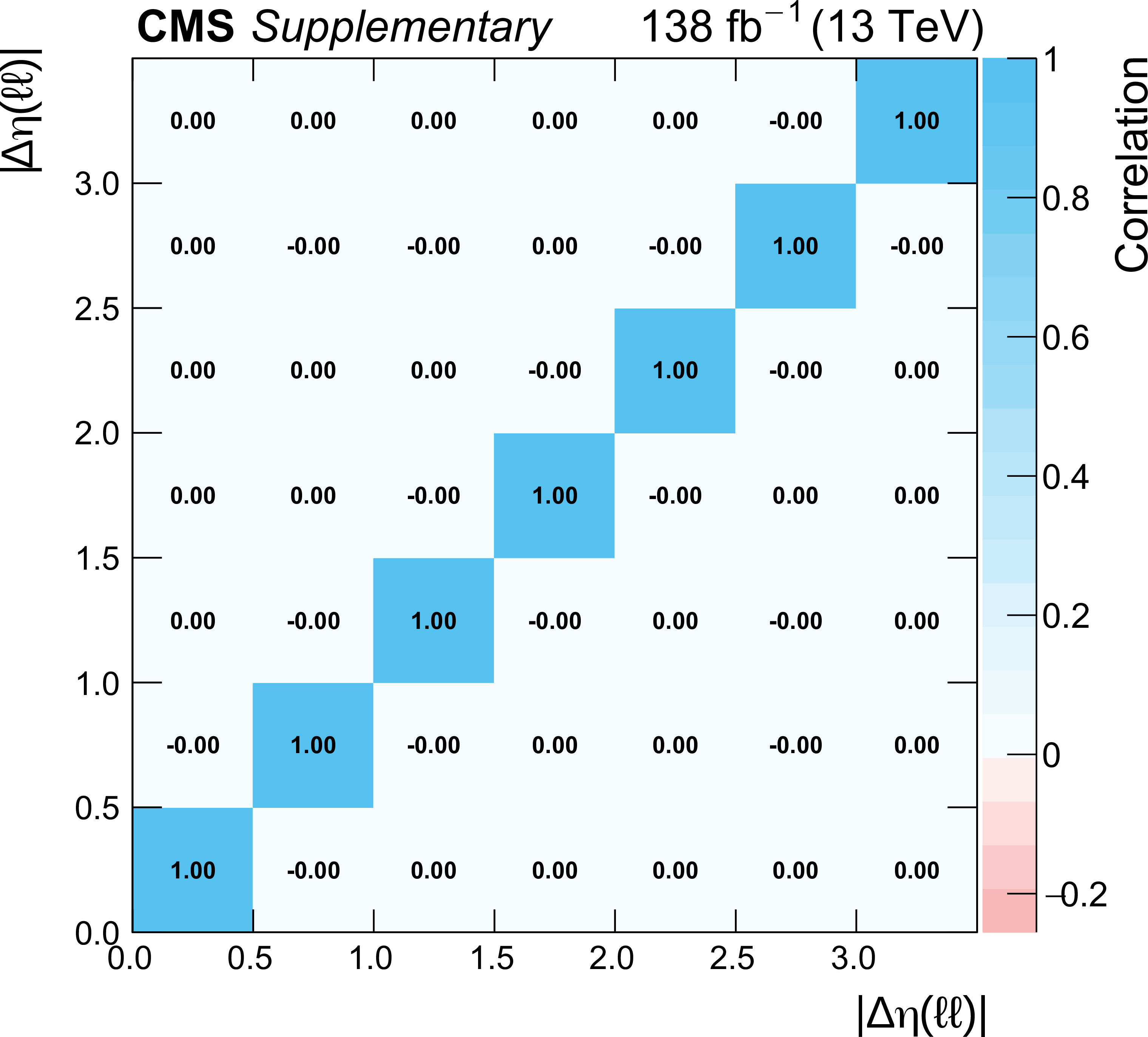
png pdf |
Additional Figure 21:
Statistical correlation between the bins of the measured absolute differential cross section as a function of $ {| \Delta \eta (\ell \ell) |}$. |
png pdf |
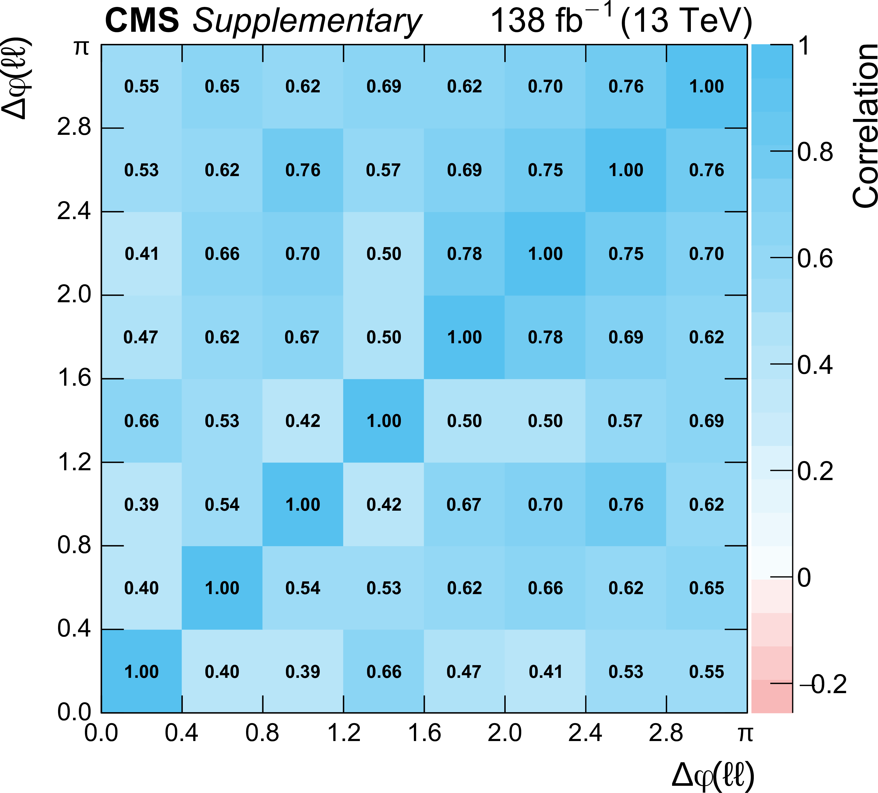
Additional Figure 22:
Systematic correlation between the bins of the measured absolute differential cross section as a function of $\Delta \varphi (\ell \ell)$. |
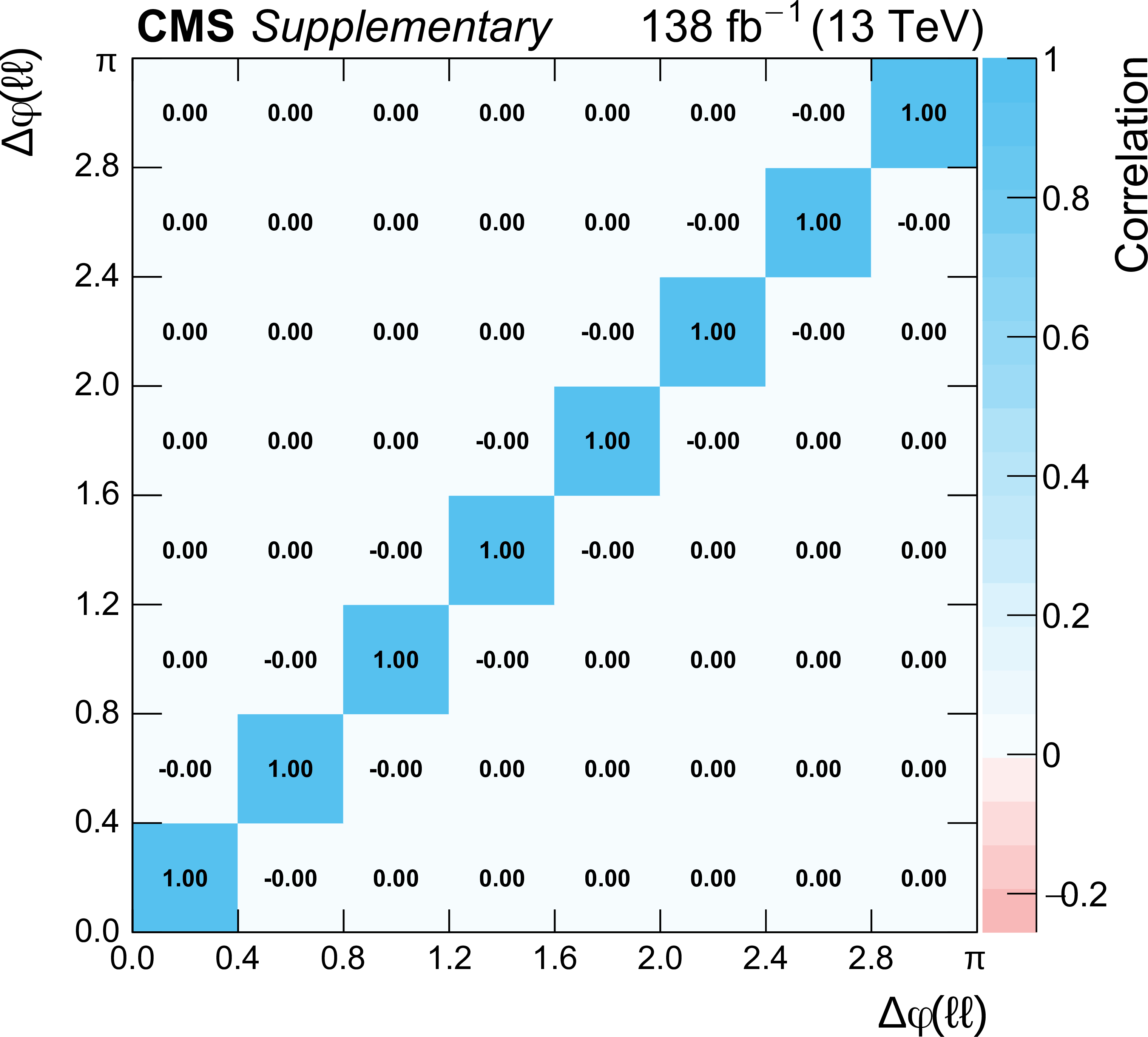
png pdf |
Additional Figure 23:
Statistical correlation between the bins of the measured absolute differential cross section as a function of $\Delta \varphi (\ell \ell)$. |
png pdf |
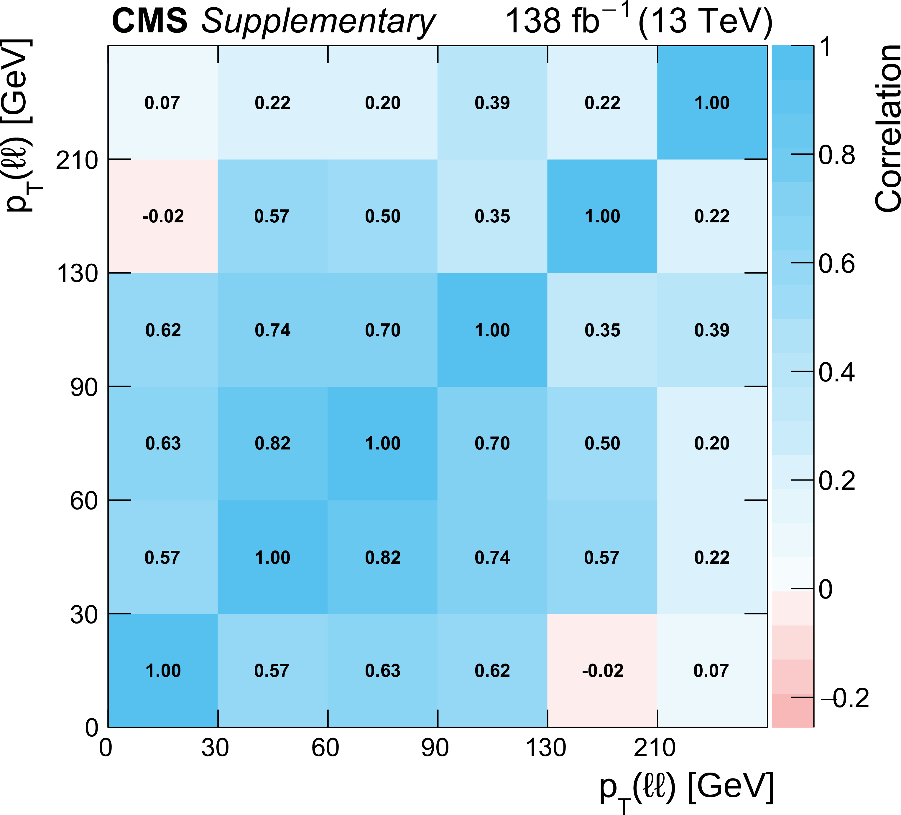
Additional Figure 24:
Systematic correlation between the bins of the measured absolute differential cross section as a function of $ {p_{\mathrm {T}}} (\ell \ell)$. |
png pdf |
Additional Figure 25:
Statistical correlation between the bins of the measured absolute differential cross section as a function of $ {p_{\mathrm {T}}} (\ell \ell)$. |
png pdf |
Additional Figure 26:
Systematic correlation between the bins of the measured absolute differential cross section as a function of $ {p_{\mathrm {T}}} (\ell _1)+ {p_{\mathrm {T}}} (\ell _2)$. |
png pdf |
Additional Figure 27:
Statistical correlation between the bins of the measured absolute differential cross section as a function of $ {p_{\mathrm {T}}} (\ell _1)+ {p_{\mathrm {T}}} (\ell _2)$. |
png pdf |
Additional Figure 28:
Systematic correlation between the bins of the measured absolute differential cross section as a function of $\min {\Delta R}(\ell,\mathrm {j})$. |

png pdf |
Additional Figure 29:
Statistical correlation between the bins of the measured absolute differential cross section as a function of $\min {\Delta R}(\ell,\mathrm {j})$. |
png pdf |
Additional Figure 30:
Systematic correlation between the bins of the measured absolute differential cross section as a function of $ {p_{\mathrm {T}}} (\mathrm {j}_1)$. |
png pdf |
Additional Figure 31:
Statistical correlation between the bins of the measured absolute differential cross section as a function of $ {p_{\mathrm {T}}} (\mathrm {j}_1)$. |
png pdf |
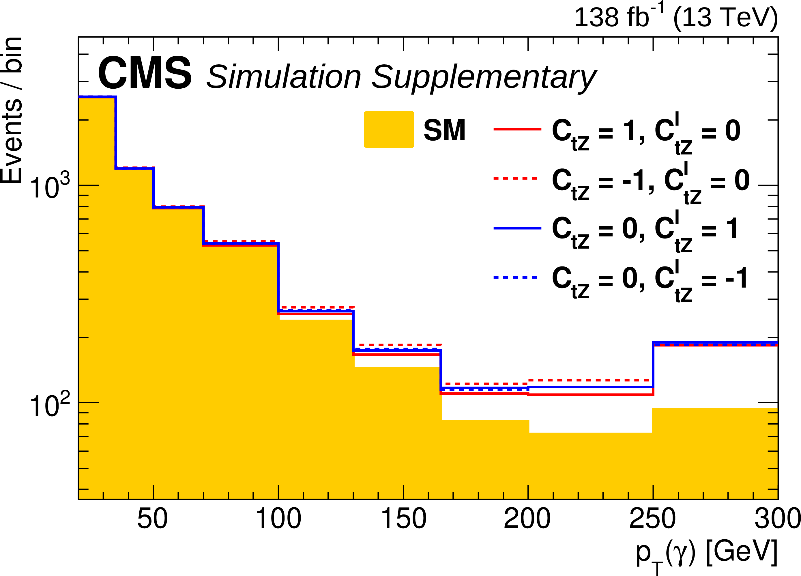
Additional Figure 32:
Predicted photon ${p_{\mathrm {T}}}$ distribution of the ${\mathrm{t} {}\mathrm{\bar{t}}} \gamma $ signal process in the signal selection, compared for the SM prediction (shaded yellow) and predictions with nonzero Wilson coefficients $c_{\mathrm{t} \mathrm{Z}}$ (red lines) or $c_{\mathrm{t} \mathrm{Z}}^{\mathrm {I}}$ (blue lines). The definition of the Wilson coefficients can be found in the article. |
png pdf |
Additional Figure 33:
Distributions of the observed (solid line) and expected (dashed line) negative log-likelihood difference from the best fit value for the one-dimensional scan of the Wilson coefficient $c_{\mathrm{t} \mathrm{Z}}$ using the photon ${p_{\mathrm {T}}}$ distribution from this analysis. In the scans, the Wilson coefficient $c_{\mathrm{t} \mathrm{Z}}^{\mathrm {I}}$ is profiled. The green (orange) bands indicate the 68 (95)% CL limits on the Wilson coefficient. The definition of the Wilson coefficients can be found in the article. |

png pdf |
Additional Figure 34:
Distributions of the observed (solid line) and expected (dashed line) negative log-likelihood difference from the best fit value for the one-dimensional scan of the Wilson coefficient $c_{\mathrm{t} \mathrm{Z}}$ using the photon ${p_{\mathrm {T}}}$ distribution from the combination of this analysis with the $\ell $+jets analysis. In the scans, the Wilson coefficient $c_{\mathrm{t} \mathrm{Z}}^{\mathrm {I}}$ is profiled. The green (orange) bands indicate the 68 (95)% CL limits on the Wilson coefficient. The definition of the Wilson coefficients can be found in the article. |

png pdf |
Additional Figure 35:
Distributions of the observed (solid line) and expected (dashed line) negative log-likelihood difference from the best fit value for the one-dimensional scan of the Wilson coefficient $c_{\mathrm{t} \mathrm{Z}}^{\mathrm {I}}$, using the photon ${p_{\mathrm {T}}}$ distribution from this analysis. In the scans, the Wilson coefficient $c_{\mathrm{t} \mathrm{Z}}$ is profiled. The green (orange) bands indicate the 68 (95)% CL limits on the Wilson coefficient. The definition of the Wilson coefficients can be found in the article. |

png pdf |
Additional Figure 36:
Distributions of the observed (solid line) and expected (dashed line) negative log-likelihood difference from the best fit value for the one-dimensional scan of the Wilson coefficient $c_{\mathrm{t} \mathrm{Z}}^{\mathrm {I}}$, using the photon ${p_{\mathrm {T}}}$ distribution from the combination of this analysis with the $\ell $+jets analysis. In the scans, the Wilson coefficient $c_{\mathrm{t} \mathrm{Z}}$ is profiled. The green (orange) bands indicate the 68 (95)% CL limits on the Wilson coefficient. The definition of the Wilson coefficients can be found in the article. |
| References | ||||
| 1 | CDF Collaboration | Evidence for $ \mathrm{t\bar{t}}\gamma $ production and measurement of $ \sigma_{\mathrm{t\bar{t}}\gamma}/\sigma_{\mathrm{t\bar{t}}} $ | PRD 84 (2011) 031104 | 1106.3970 |
| 2 | ATLAS Collaboration | Observation of top-quark pair production in association with a photon and measurement of the $ \mathrm{t\bar{t}}\gamma $ production cross section in pp collisions at $\sqrt{s}=$ 7 TeV using the ATLAS detector | PRD 91 (2015) 072007 | 1502.00586 |
| 3 | ATLAS Collaboration | Measurement of the $ \mathrm{t\bar{t}}\gamma $ production cross section in proton-proton collisions at $\sqrt{s}=$ 8 TeV with the ATLAS detector | JHEP 11 (2017) 086 | 1706.03046 |
| 4 | CMS Collaboration | Measurement of the semileptonic $ \mathrm{t\bar{t}}+{\gamma} $ production cross section in pp collisions at $\sqrt{s}=$ 8 TeV | JHEP 10 (2017) 006 | CMS-TOP-14-008 1706.08128 |
| 5 | ATLAS Collaboration | Measurements of inclusive and differential fiducial cross-sections of $ \mathrm{t\bar{t}}\gamma $ production in leptonic final states at $\sqrt{s}=$ 13 TeV in ATLAS | EPJC 79 (2019) 382 | 1812.01697 |
| 6 | ATLAS Collaboration | Measurements of inclusive and differential cross-sections of combined $ \mathrm{t\bar{t}}\gamma $ and $ {\mathrm{t}\mathrm{W}\gamma} $ production in the e$\mu$ channel at 13 TeV with the ATLAS detector | JHEP 09 (2020) 049 | 2007.06946 |
| 7 | CMS Collaboration | Measurement of the inclusive and differential $ \mathrm{t\bar{t}}\gamma $ cross sections in the single-lepton channel and EFT interpretation at $\sqrt{s}=$ 13 TeV | JHEP 12 (2021) 180 | CMS-TOP-18-010 2107.01508 |
| 8 | W. Buchmuller and D. Wyler | Effective lagrangian analysis of new interactions and flavour conservation | NPB 268 (1986) 621 | |
| 9 | B. Grzadkowski, M. Iskrzyński, M. Misiak, and J. Rosiek | Dimension-six terms in the standard model Lagrangian | JHEP 10 (2010) 085 | 1008.4884 |
| 10 | P.-F. Duan et al. | QCD corrections to associated production of $ \mathrm{t\bar{t}}\gamma $ at hadron colliders | PRD 80 (2009) 014022 | 0907.1324 |
| 11 | K. Melnikov, M. Schulze, and A. Scharf | QCD corrections to top quark pair production in association with a photon at hadron colliders | PRD 83 (2011) 074013 | 1102.1967 |
| 12 | P.-F. Duan et al. | Next-to-leading order QCD corrections to $ \mathrm{t\bar{t}}\gamma $ production at the 7 TeV LHC | Chin. PL28 (2011) 111401 | 1110.2315 |
| 13 | A. Kardos and Z. Trócsányi | Hadroproduction of $ \mathrm{t\bar{t}} $ pair in association with an isolated photon at NLO accuracy matched with parton shower | JHEP 05 (2015) 090 | 1406.2324 |
| 14 | F. Maltoni, D. Pagani, and I. Tsinikos | Associated production of a top-quark pair with vector bosons at NLO in QCD: impact on $\mathrm{t\bar{t}}$H searches at the LHC | JHEP 02 (2016) 113 | 1507.05640 |
| 15 | P.-F. Duan et al. | Electroweak corrections to top quark pair production in association with a hard photon at hadron colliders | PLB 766 (2017) 102 | 1612.00248 |
| 16 | D. Pagani, H.-S. Shao, I. Tsinikos, and M. Zaro | Automated EW corrections with isolated photons: $ \mathrm{t\bar{t}}\gamma, {\mathrm{t\bar{t}}\gamma\gamma} $ and $ {\mathrm{t}\gamma\text{j}} $ as case studies | JHEP 09 (2021) 155 | 2106.02059 |
| 17 | G. Bevilacqua et al. | Precise predictions for $ {\mathrm{t\bar{t}}\gamma}/\mathrm{t\bar{t}} $ cross section ratios at the LHC | JHEP 01 (2019) 188 | 1809.08562 |
| 18 | G. Bevilacqua et al. | Off-shell vs on-shell modelling of top quarks in photon associated production | JHEP 03 (2020) 154 | 1912.09999 |
| 19 | U. Baur, A. Juste, L. H. Orr, and D. Rainwater | Probing electroweak top quark couplings at hadron colliders | PRD 71 (2005) 054013 | hep-ph/0412021 |
| 20 | A. Bouzas and F. Larios | Electromagnetic dipole moments of the top quark | PRD 87 (2013) 074015 | 1212.6575 |
| 21 | M. Schulze and Y. Soreq | Pinning down electroweak dipole operators of the top quark | EPJC 76 (2016) 466 | 1603.08911 |
| 22 | O. Bessidskaia Bylund et al. | Probing top quark neutral couplings in the standard model effective field theory at NLO in QCD | JHEP 05 (2016) 052 | 1601.08193 |
| 23 | J. A. Aguilar-Saavedra, E. Álvarez, A. Juste, and F. Rubbo | Shedding light on the $ \mathrm{t\bar{t}} $ asymmetry: the photon handle | JHEP 04 (2014) 188 | 1402.3598 |
| 24 | J. Bergner and M. Schulze | The top quark charge asymmetry in $ \mathrm{t\bar{t}}\gamma $ production at the LHC | EPJC 79 (2019) 189 | 1812.10535 |
| 25 | CMS Collaboration | HEPData record for this analysis | link | |
| 26 | CMS Collaboration | The CMS experiment at the CERN LHC | JINST 3 (2008) S08004 | CMS-00-001 |
| 27 | CMS Collaboration | Performance of the CMS Level-one trigger in proton-proton collisions at $\sqrt{s}=$ 13 TeV | JINST 15 (2020) P10017 | CMS-TRG-17-001 2006.10165 |
| 28 | CMS Collaboration | The CMS trigger system | JINST 12 (2017) P01020 | CMS-TRG-12-001 1609.02366 |
| 29 | J. Alwall et al. | The automated computation of tree-level and next-to-leading order differential cross sections, and their matching to parton shower simulations | JHEP 07 (2014) 079 | 1405.0301 |
| 30 | NNPDF Collaboration | Parton distributions from high-precision collider data | EPJC 77 (2017) 663 | 1706.00428 |
| 31 | P. Nason | A new method for combining NLO QCD with shower Monte Carlo algorithms | JHEP 11 (2004) 040 | hep-ph/0409146 |
| 32 | S. Frixione, G. Ridolfi, and P. Nason | A positive-weight next-to-leading-order Monte Carlo for heavy flavour hadroproduction | JHEP 09 (2007) 126 | 0707.3088 |
| 33 | S. Frixione, P. Nason, and C. Oleari | Matching NLO QCD computations with parton shower simulations: the POWHEG method | JHEP 11 (2007) 070 | 0709.2092 |
| 34 | S. Alioli, P. Nason, C. Oleari, and E. Re | NLO single-top production matched with shower in POWHEG: s- and t-channel contributions | JHEP 09 (2009) 111 | 0907.4076 |
| 35 | S. Alioli, P. Nason, C. Oleari, and E. Re | A general framework for implementing NLO calculations in shower Monte Carlo programs: the POWHEG box | JHEP 06 (2010) 043 | 1002.2581 |
| 36 | E. Re | Single-top Wt-channel production matched with parton showers using the POWHEG method | EPJC 71 (2011) 1547 | 1009.2450 |
| 37 | J. M. Campbell, R. K. Ellis, P. Nason, and E. Re | Top-pair production and decay at NLO matched with parton showers | JHEP 04 (2015) 114 | 1412.1828 |
| 38 | H. Hartanto, B. Jager, L. Reina, and D. Wackeroth | Higgs boson production in association with top quarks in the POWHEG box | PRD 91 (2015) 094003 | 1501.04498 |
| 39 | J. M. Campbell and R. K. Ellis | MCFM for the Tevatron and the LHC | NPB Proc. Suppl. 205-206 (2010) 10 | 1007.3492 |
| 40 | J. M. Campbell, R. K. Ellis, and C. Williams | Bounding the Higgs width at the LHC using full analytic results for $ {\mathrm{g}\mathrm{g}}\to{\mathrm{e^{-}}\mathrm{e^{+}}\mu^{-}\mu^{+}} $ | JHEP 04 (2014) 060 | 1311.3589 |
| 41 | NNPDF Collaboration | Parton distributions for the LHC Run II | JHEP 04 (2015) 040 | 1410.8849 |
| 42 | T. Sjostrand et al. | An introduction to PYTHIA 8.2 | CPC 191 (2015) 159 | 1410.3012 |
| 43 | CMS Collaboration | Extraction and validation of a new set of CMS PYTHIA 8 tunes from underlying-event measurements | EPJC 80 (2020) 4 | CMS-GEN-17-001 1903.12179 |
| 44 | P. Skands, S. Carrazza, and J. Rojo | Tuning PYTHIA 8.1: the Monash 2013 tune | EPJC 74 (2014) 3024 | 1404.5630 |
| 45 | CMS Collaboration | Event generator tunes obtained from underlying event and multiparton scattering measurements | EPJC 76 (2016) 155 | CMS-GEN-14-001 1512.00815 |
| 46 | CMS Collaboration | Investigations of the impact of the parton shower tuning in PYTHIA 8 in the modelling of $ \mathrm{t\bar{t}} $ at $ \sqrt{s}= $ 8 and 13 TeV | CMS-PAS-TOP-16-021 | CMS-PAS-TOP-16-021 |
| 47 | J. Alwall et al. | Comparative study of various algorithms for the merging of parton showers and matrix elements in hadronic collisions | EPJC 53 (2008) 473 | 0706.2569 |
| 48 | R. Frederix and S. Frixione | Merging meets matching in MCatNLO | JHEP 12 (2012) 061 | 1209.6215 |
| 49 | Y. Li and F. Petriello | Combining QCD and electroweak corrections to dilepton production in FEWZ | PRD 86 (2012) 094034 | 1208.5967 |
| 50 | M. Czakon and A. Mitov | TOP++: A program for the calculation of the top-pair cross-section at hadron colliders | CPC 185 (2014) 2930 | 1112.5675 |
| 51 | M. Aliev et al. | HATHOR: Hadronic top and heavy quarks cross section calculator | CPC 182 (2011) 1034 | 1007.1327 |
| 52 | P. Kant et al. | HATHOR: for single top-quark production: Updated predictions and uncertainty estimates for single top-quark production in hadronic collisions | CPC 191 (2015) 74 | 1406.4403 |
| 53 | N. Kidonakis | Theoretical results for electroweak boson and single-top production | in XXIII International Workshop on Deep-Inelastic Scattering (DIS2015) 2015 | 1506.04072 |
| 54 | CMS Collaboration | Object definitions for top quark analyses at the particle level | CDS | |
| 55 | M. Cacciari, G. P. Salam, and G. Soyez | The anti-$ {k_{\mathrm{T}}} $ jet clustering algorithm | JHEP 04 (2008) 063 | 0802.1189 |
| 56 | M. Cacciari, G. P. Salam, and G. Soyez | The catchment area of jets | JHEP 04 (2008) 005 | 0802.1188 |
| 57 | GEANT4 Collaboration | GEANT4--a simulation toolkit | NIMA 506 (2003) 250 | |
| 58 | CMS Collaboration | Particle-flow reconstruction and global event description with the CMS detector | JINST 12 (2017) P10003 | CMS-PRF-14-001 1706.04965 |
| 59 | M. Cacciari, G. P. Salam, and G. Soyez | FastJet user manual | EPJC 72 (2012) 1896 | 1111.6097 |
| 60 | CMS Collaboration | Electron and photon reconstruction and identification with the CMS experiment at the CERN LHC | JINST 16 (2021) P05014 | CMS-EGM-17-001 2012.06888 |
| 61 | CMS Collaboration | Performance of the CMS muon detector and muon reconstruction with proton-proton collisions at $\sqrt{s}=$ 13 TeV | JINST 13 (2018) P06015 | CMS-MUO-16-001 1804.04528 |
| 62 | CMS Collaboration | Inclusive and differential cross section measurements of single top quark production in association with a Z boson in proton-proton collisions at $\sqrt{s}=$ 13 TeV | 2021. Submitted to JHEP | CMS-TOP-20-010 2111.02860 |
| 63 | A. Hoecker et al. | TMVA---Toolkit for multivariate data analysis | 2007 | physics/0703039 |
| 64 | CMS Collaboration | Pileup mitigation at CMS in 13 TeV data | JINST 15 (2020) P09018 | CMS-JME-18-001 2003.00503 |
| 65 | CMS Collaboration | Jet energy scale and resolution in the CMS experiment in pp collisions at 8 TeV | JINST 12 (2017) P02014 | CMS-JME-13-004 1607.03663 |
| 66 | CMS Collaboration | Identification of heavy-flavour jets with the CMS detector in pp collisions at 13 TeV | JINST 13 (2018) P05011 | CMS-BTV-16-002 1712.07158 |
| 67 | Particle Data Group, P. A. Zyla et al. | Review of particle physics | Prog. Theor. Exp. Phys. 2020 (2020) 083C01 | |
| 68 | CMS Collaboration | Search for WW$ \gamma $ and WZ$ \gamma $ production and constraints on anomalous quartic gauge couplings in pp collisions at $\sqrt{s}=$ 8 TeV | PRD 90 (2014) 032008 | CMS-SMP-13-009 1404.4619 |
| 69 | ATLAS Collaboration | Measurements of Z$ \gamma $ and Z$ \gamma\gamma $ production in pp collisions at $\sqrt{s}=$ 8 TeV with the ATLAS detector | PRD 93 (2016) 112002 | 1604.05232 |
| 70 | CMS Collaboration | Measurement of the production cross section for single top quarks in association with W bosons in proton-proton collisions at $\sqrt{s}=$ 13 TeV | JHEP 10 (2018) 117 | CMS-TOP-17-018 1805.07399 |
| 71 | CMS Collaboration | Precision luminosity measurement in proton-proton collisions at $\sqrt{s}=$ 13 TeV in 2015 and 2016 at CMS | EPJC 81 (2021) 800 | CMS-LUM-17-003 2104.01927 |
| 72 | CMS Collaboration | CMS luminosity measurement for the 2017 data-taking period at $\sqrt{s}=$ 13 TeV | CMS-PAS-LUM-17-004 | CMS-PAS-LUM-17-004 |
| 73 | CMS Collaboration | CMS luminosity measurement for the 2018 data-taking period at $\sqrt{s}=$ 13 TeV | CMS-PAS-LUM-18-002 | CMS-PAS-LUM-18-002 |
| 74 | J. Butterworth et al. | PDF4LHC recommendations for LHC Run II | JPG 43 (2016) 023001 | 1510.03865 |
| 75 | S. Argyropoulos and T. Sjostrand | Effects of color reconnection on $ \mathrm{t\bar{t}} $ final states at the LHC | JHEP 11 (2014) 043 | 1407.6653 |
| 76 | J. Christiansen and P. Skands | String formation beyond leading colour | JHEP 08 (2015) 003 | 1505.01681 |
| 77 | M. Bowler | $ \mathrm{e^{+}e^{-}} $ production of heavy quarks in the string model | Z. Phys. C 11 (1981) 169 | |
| 78 | ATLAS Collaboration, CMS Collaboration, and LHC Higgs Combination Group | Procedure for the LHC Higgs boson search combination in Summer 2011 | CMS-NOTE-2011-005 | |
| 79 | G. Cowan, K. Cranmer, E. Gross, and O. Vitells | Asymptotic formulae for likelihood-based tests of new physics | EPJC 71 (2011) 1554 | 1007.1727 |
| 80 | CMS Collaboration | Measurement of the $ \mathrm{t\bar{t}} $ production cross section, the top quark mass, and the strong coupling constant using dilepton events in pp collisions at $\sqrt{s}=$ 13 TeV | EPJC 79 (2019) 368 | CMS-TOP-17-001 1812.10505 |
| 81 | G. Cowan | Statistical data analysis | Clarendon Press, Oxford U.K., 1998 ISBN 978-0-19-850156-5 | |
| 82 | S. Schmitt | TUnfold, an algorithm for correcting migration effects in high energy physics | JINST 7 (2012) T10003 | 1205.6201 |
| 83 | J. Bellm et al. | HERWIG 7.0/HERWIG++ 3.0 release note | EPJC 76 (2016) 196 | 1512.01178 |
| 84 | CMS Collaboration | Development and validation of HERWIG 7 tunes from CMS underlying-event measurements | EPJC 81 (2021) 312 | CMS-GEN-19-001 2011.03422 |
| 85 | CMS Collaboration | Measurements of $ \mathrm{t\bar{t}} $ differential cross sections in proton-proton collisions at $\sqrt{s}=$ 13 TeV using events containing two leptons | JHEP 02 (2019) 149 | CMS-TOP-17-014 1811.06625 |
| 86 | CMS Collaboration | Measurement of the top quark polarization and $ \mathrm{t\bar{t}} $ spin correlations using dilepton final states in proton-proton collisions at $\sqrt{s}=$ 13 TeV | PRD 100 (2019) 072002 | CMS-TOP-18-006 1907.03729 |
| 87 | A. Helset and A. Kobach | Baryon number, lepton number, and operator dimension in the SMEFT with flavor symmetries | PLB 800 (2020) 135132 | 1909.05853 |
| 88 | J. A. Aguilar-Saavedra et al. | Interpreting top-quark LHC measurements in the standard-model effective field theory | LHC TOP WG note CERN-LPCC-2018-01 | 1802.07237 |
| 89 | J. A. Aguilar-Saavedra | A minimal set of top anomalous couplings | NPB 812 (2009) 181 | 0811.3842 |
| 90 | C. Zhang and S. Willenbrock | Effective-field-theory approach to top-quark production and decay | PRD 83 (2011) 034006 | 1008.3869 |
| 91 | ATLAS and CMS Collaborations | Combination of the W boson polarization measurements in top quark decays using ATLAS and CMS data at $\sqrt{s}=$ 8 TeV | JHEP 08 (2020) 051 | 2005.03799 |
| 92 | CMS Collaboration | Measurement of the cross section for top quark pair production in association with a W or Z boson in proton-proton collisions at $\sqrt{s}=$ 13 TeV | JHEP 08 (2018) 011 | CMS-TOP-17-005 1711.02547 |
| 93 | ATLAS Collaboration | Measurement of the $\mathrm{t\bar{t}}$Z and $\mathrm{t\bar{t}}$W cross sections in proton-proton collisions at $\sqrt{s}=$ 13 TeV with the ATLAS detector | PRD 99 (2019) 072009 | 1901.03584 |
| 94 | CMS Collaboration | Measurement of top quark pair production in association with a Z boson in proton-proton collisions at $\sqrt{s}=$ 13 TeV | JHEP 03 (2020) 056 | CMS-TOP-18-009 1907.11270 |
| 95 | CMS Collaboration | Search for new physics in top quark production with additional leptons in proton-proton collisions at $\sqrt{s}=$ 13 TeV using effective field theory | JHEP 03 (2021) 095 | CMS-TOP-19-001 2012.04120 |
| 96 | CMS Collaboration | Probing effective field theory operators in the associated production of top quarks with a Z boson in multilepton final states at $\sqrt{s}=$ 13 TeV | JHEP 12 (2021) 083 | CMS-TOP-21-001 2107.13896 |
| 97 | N. Hartland et al. | A Monte Carlo global analysis of the standard model effective field theory: the top quark sector | JHEP 04 (2019) 100 | 1901.05965 |
| 98 | I. Brivio et al. | O new physics, where art thou? A global search in the top sector | JHEP 02 (2020) 131 | 1910.03606 |
| 99 | J. Ellis et al. | Top, Higgs, diboson and electroweak fit to the standard model effective field theory | JHEP 04 (2021) 279 | 2012.02779 |
| 100 | S. Bißmann, C. Grunwald, G. Hiller, and K. Kroninger | Top and beauty synergies in SMEFT-fits at present and future colliders | JHEP 06 (2021) 010 | 2012.10456 |
| 101 | J. Ethier et al. | Combined SMEFT interpretation of Higgs, diboson, and top quark data from the LHC | JHEP 11 (2021) 089 | 2105.00006 |
|
|
Compact Muon Solenoid LHC, CERN |
|

|

|

|

|

|