

Compact Muon Solenoid
LHC, CERN
| CMS-HIG-21-001 ; CERN-EP-2022-137 | ||
| Searches for additional Higgs bosons and for vector leptoquarks in $\tau\tau$ final states in proton-proton collisions at $\sqrt{s} = $ 13 TeV | ||
| CMS Collaboration | ||
| 4 August 2022 | ||
| JHEP 07 (2023) 073 | ||
| Abstract: Three searches are presented for signatures of physics beyond the standard model (SM) in $\tau\tau$ final states in proton-proton collisions at the LHC, using a data sample collected with the CMS detector at $\sqrt{s} = $ 13 TeV, corresponding to an integrated luminosity of 138 fb$^{-1}$. Upper limits at 95% confidence level (CL) are set on the products of the branching fraction for the decay into $\tau$ leptons and the cross sections for the production of a new boson $\phi$, in addition to the H(125) boson, via gluon fusion (gg$\phi$) or in association with b quarks, ranging from ${\mathcal{O}}$(10 pb) for a mass of 60 GeV to 0.3 fb for a mass of 3.5 TeV each. The data reveal two excesses for gg$\phi$ production with local $p$-values equivalent to about three standard deviations at ${m_{\phi}} =$ 0.1 and 1.2 TeV. In a search for $t$-channel exchange of a vector leptoquark U$_{1}$, 95% CL upper limits are set on the dimensionless U$_{1}$ leptoquark coupling to quarks and $\tau$ leptons ranging from 1 for a mass of 1 TeV to 6 for a mass of 5 TeV, depending on the scenario. In the interpretations of the ${M_{\mathrm{h}}^{125}}$ and ${M_{\mathrm{h},\,\text{EFT}}^{125}}$ minimal supersymmetric SM benchmark scenarios, additional Higgs bosons with masses below 350 GeV are excluded at 95% CL. | ||
| Links: e-print arXiv:2208.02717 [hep-ex] (PDF) ; CDS record ; inSPIRE record ; HepData record ; CADI line (restricted) ; | ||
| Figures & Tables | Summary | Additional Figures | References | CMS Publications |
|---|
| Figures | |
png pdf |
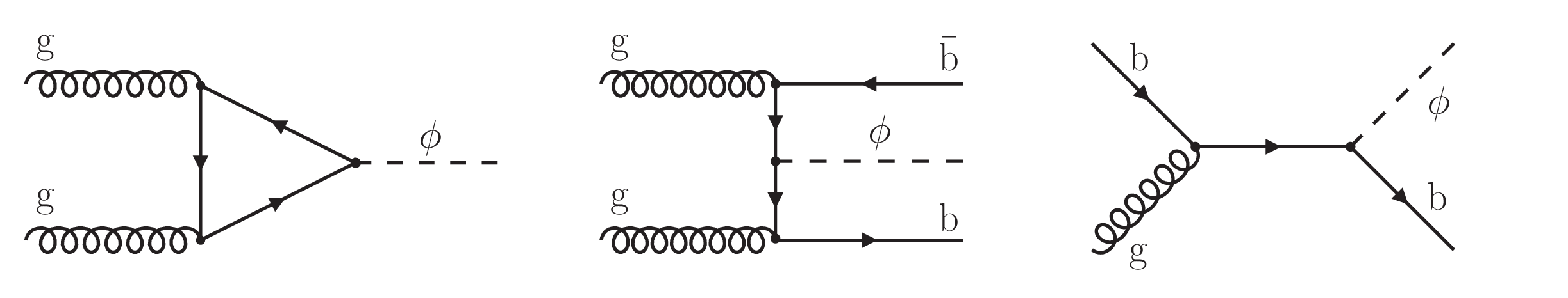
Figure 1:
Diagrams for the production of neutral Higgs bosons ${\phi}$ (left) via gluon fusion, labelled as gg$\phi$, and (middle and right) in association with b quarks, labelled as bb$\phi$ in the text. In the middle diagram, a pair of b quarks is produced from the fusion of two gluons, one from each proton. In the right diagram, a b quark from one proton scatters from a gluon from the other proton. In both cases ${\phi}$ is radiated off one of the b quarks. |
png pdf |
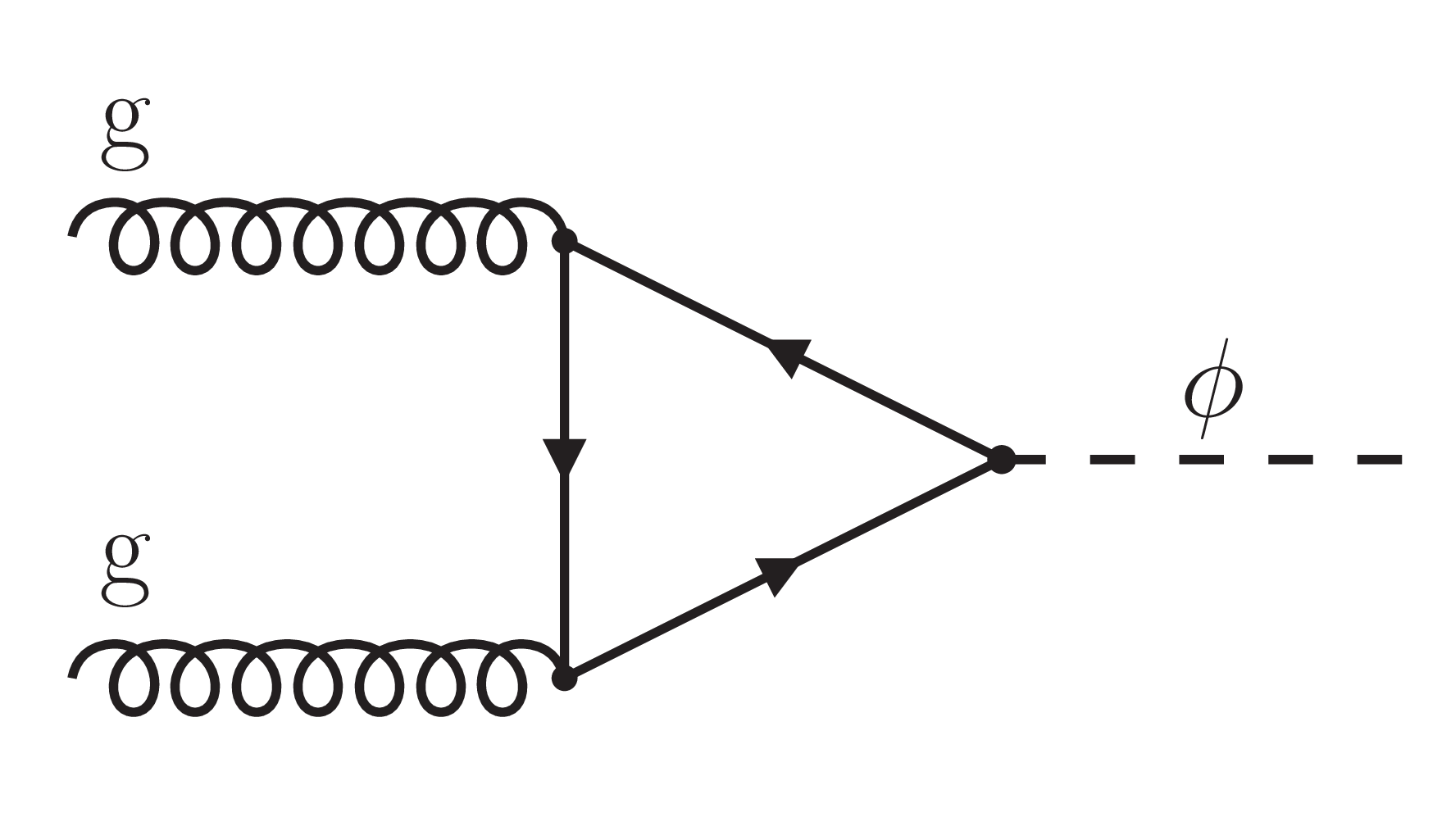
Figure 1-a:
Diagrams for the production of neutral Higgs bosons ${\phi}$ (left) via gluon fusion, labelled as gg$\phi$, and (middle and right) in association with b quarks, labelled as bb$\phi$ in the text. In the middle diagram, a pair of b quarks is produced from the fusion of two gluons, one from each proton. In the right diagram, a b quark from one proton scatters from a gluon from the other proton. In both cases ${\phi}$ is radiated off one of the b quarks. |
png pdf |
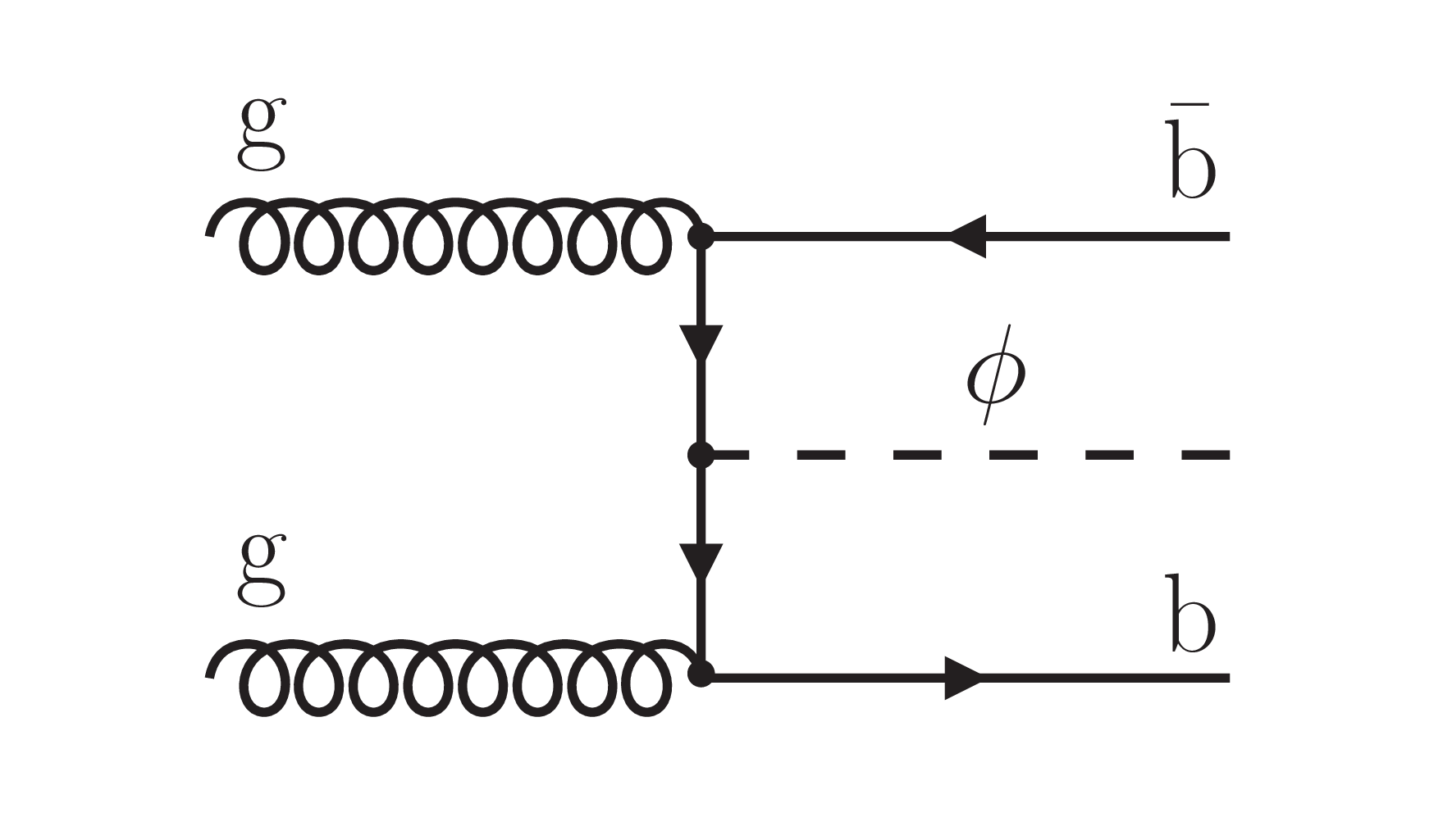
Figure 1-b:
Diagrams for the production of neutral Higgs bosons ${\phi}$ (left) via gluon fusion, labelled as gg$\phi$, and (middle and right) in association with b quarks, labelled as bb$\phi$ in the text. In the middle diagram, a pair of b quarks is produced from the fusion of two gluons, one from each proton. In the right diagram, a b quark from one proton scatters from a gluon from the other proton. In both cases ${\phi}$ is radiated off one of the b quarks. |

png pdf |
Figure 1-c:
Diagrams for the production of neutral Higgs bosons ${\phi}$ (left) via gluon fusion, labelled as gg$\phi$, and (middle and right) in association with b quarks, labelled as bb$\phi$ in the text. In the middle diagram, a pair of b quarks is produced from the fusion of two gluons, one from each proton. In the right diagram, a b quark from one proton scatters from a gluon from the other proton. In both cases ${\phi}$ is radiated off one of the b quarks. |
png pdf |
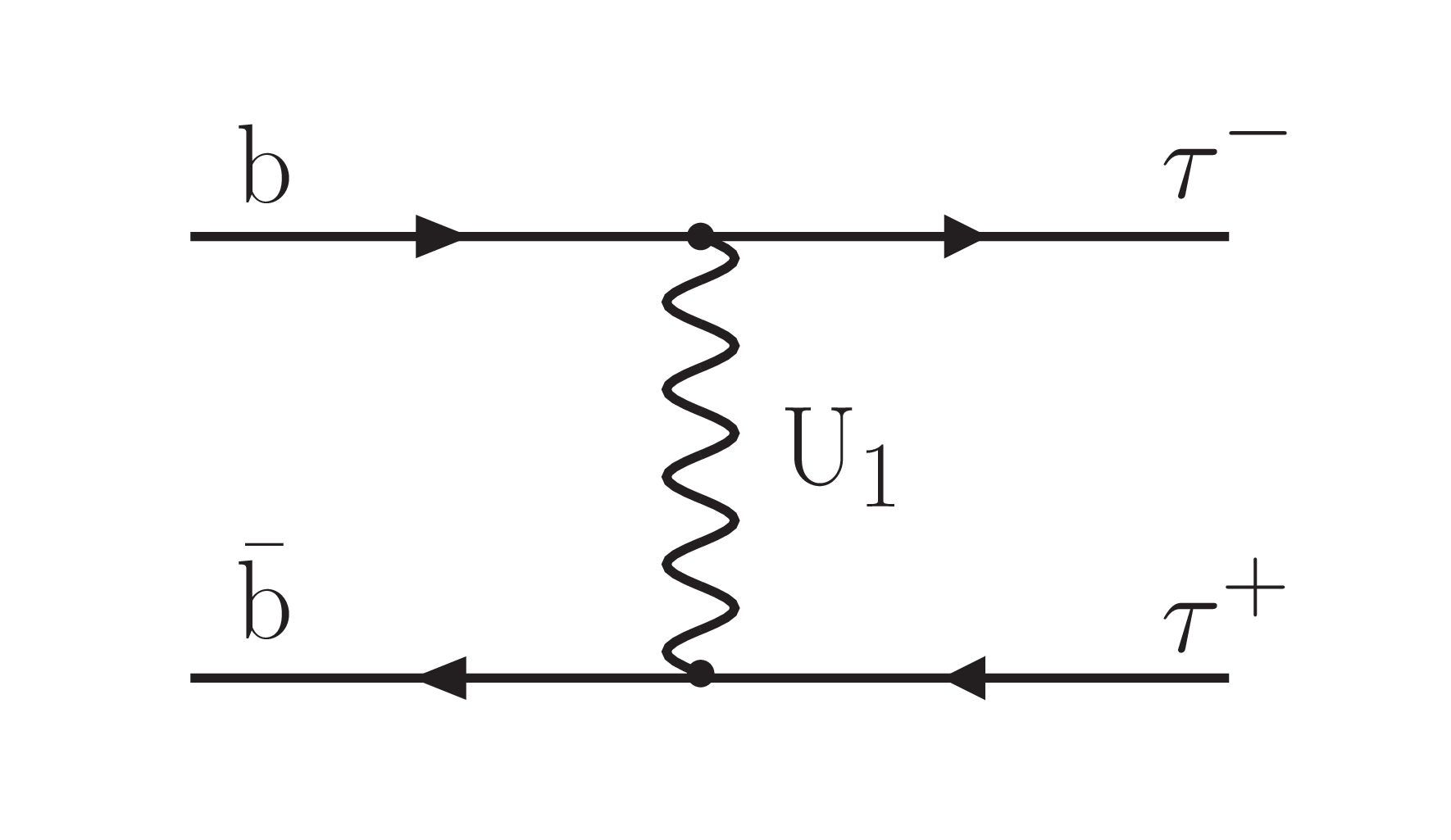
Figure 2:
Diagram for the production of a pair of $\tau$ leptons via the $t$-channel exchange of a vector leptoquark U$_{1}$. |
png pdf |
Figure 3:
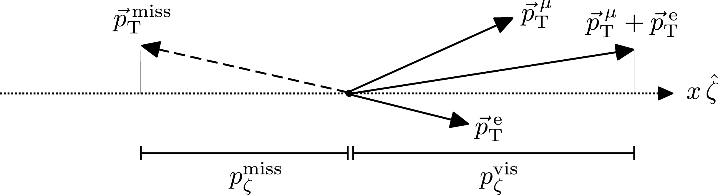
Inputs to the reconstruction of the event observable D$_{\zeta}$, as described in the text. |
png pdf |
Figure 4:
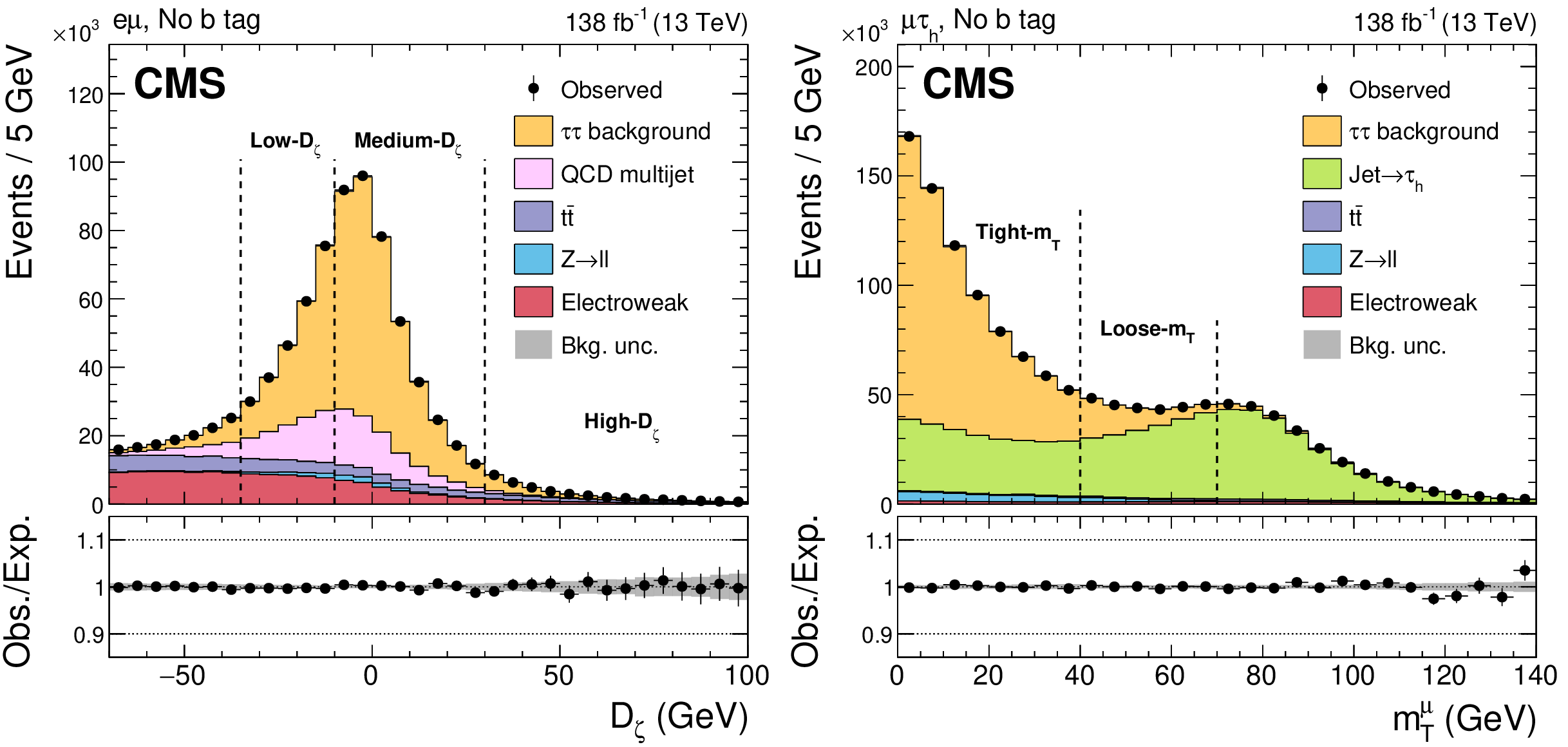
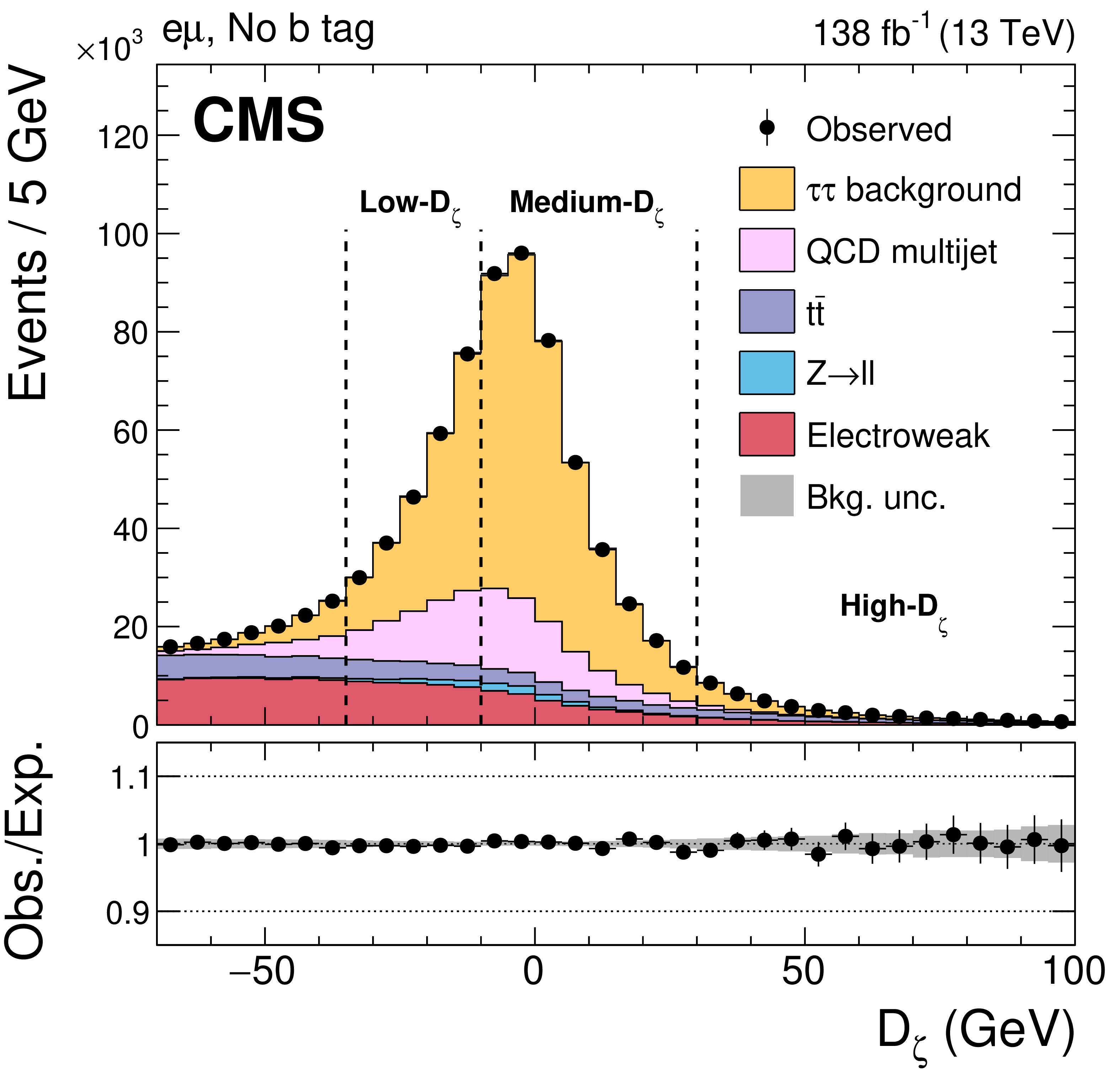
Observed and expected distributions of (left) D$_{\zeta}$ in the e$\mu$ final state and (right) ${m_{\mathrm {T}}^{\mu}}$ in the $\mu {\tau _\mathrm {h}}$ final state. The distributions are shown in the global "no b tag'' category before any further event categorization and after an individual background-only fit to the data in each corresponding variable. The grey shaded band represents the complete set of uncertainties used for signal extraction, after the fit. A detailed discussion of the data modelling is given in Section 6. The vertical dashed lines indicate the category definitions in each of the final states, as described in the text. In the lower panels of each figure the ratio of the observed numbers of events per bin to the background expectation is shown. |
png pdf |
Figure 4-a:
Observed and expected distributions of (left) D$_{\zeta}$ in the e$\mu$ final state and (right) ${m_{\mathrm {T}}^{\mu}}$ in the $\mu {\tau _\mathrm {h}}$ final state. The distributions are shown in the global "no b tag'' category before any further event categorization and after an individual background-only fit to the data in each corresponding variable. The grey shaded band represents the complete set of uncertainties used for signal extraction, after the fit. A detailed discussion of the data modelling is given in Section 6. The vertical dashed lines indicate the category definitions in each of the final states, as described in the text. In the lower panels of each figure the ratio of the observed numbers of events per bin to the background expectation is shown. |

png pdf |
Figure 4-b:
Observed and expected distributions of (left) D$_{\zeta}$ in the e$\mu$ final state and (right) ${m_{\mathrm {T}}^{\mu}}$ in the $\mu {\tau _\mathrm {h}}$ final state. The distributions are shown in the global "no b tag'' category before any further event categorization and after an individual background-only fit to the data in each corresponding variable. The grey shaded band represents the complete set of uncertainties used for signal extraction, after the fit. A detailed discussion of the data modelling is given in Section 6. The vertical dashed lines indicate the category definitions in each of the final states, as described in the text. In the lower panels of each figure the ratio of the observed numbers of events per bin to the background expectation is shown. |
png pdf |
Figure 5:
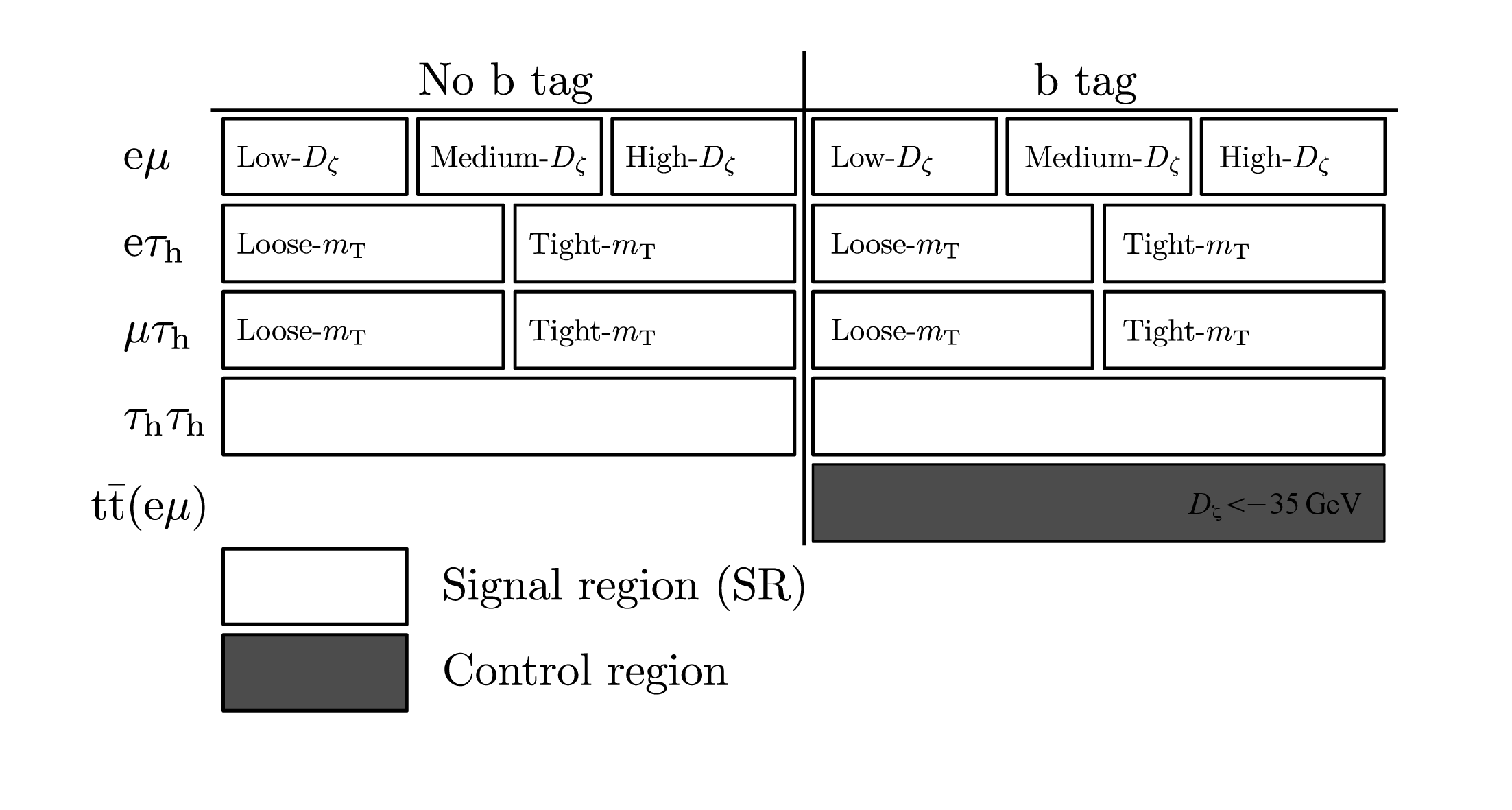
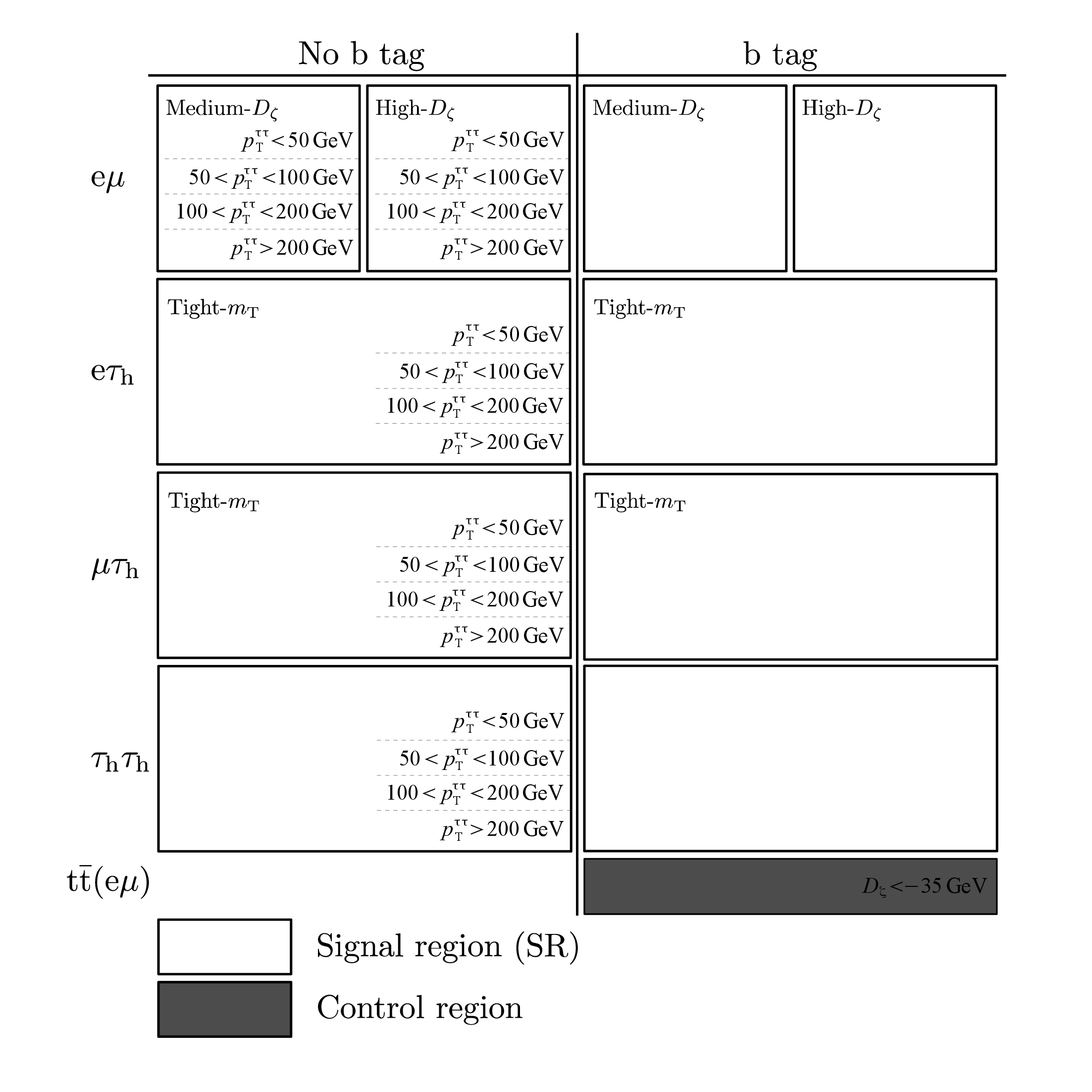
Overview of the categories used for the extraction of the signal for the model-independent ${\phi}$ search for hypothesized values of $ {m_{\phi}} \geq $ 250 GeV, the vector leptoquark search, and the interpretation of the data in MSSM benchmark scenarios. |
png pdf |
Figure 6:
Overview of the categories used for the extraction of the signal for the model-independent ${\phi}$ search for 60 $\leq {m_{\phi}} < $ 250 GeV. |
png pdf |
Figure 7:
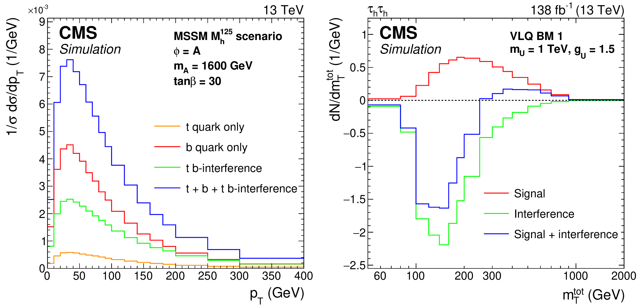
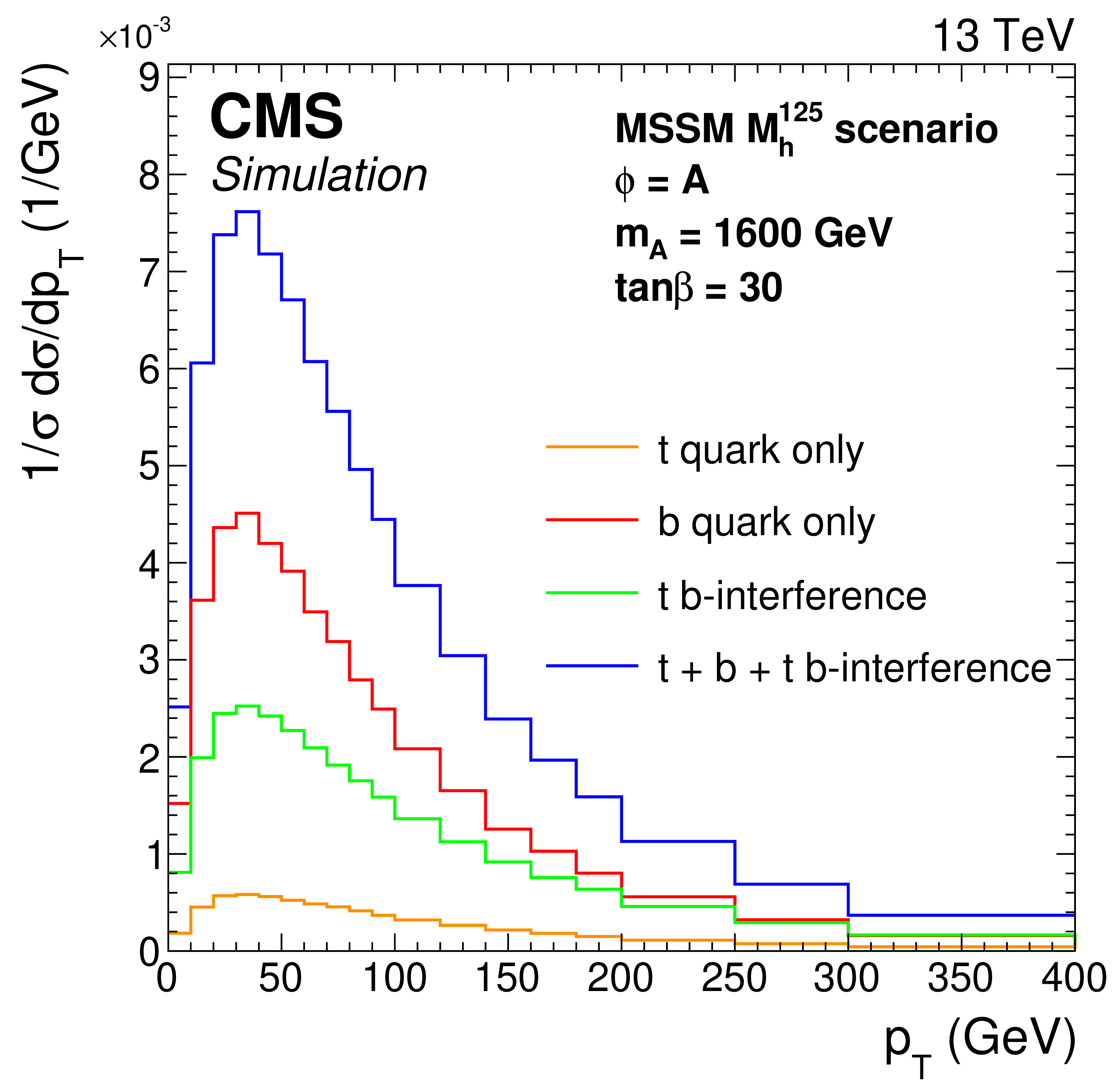
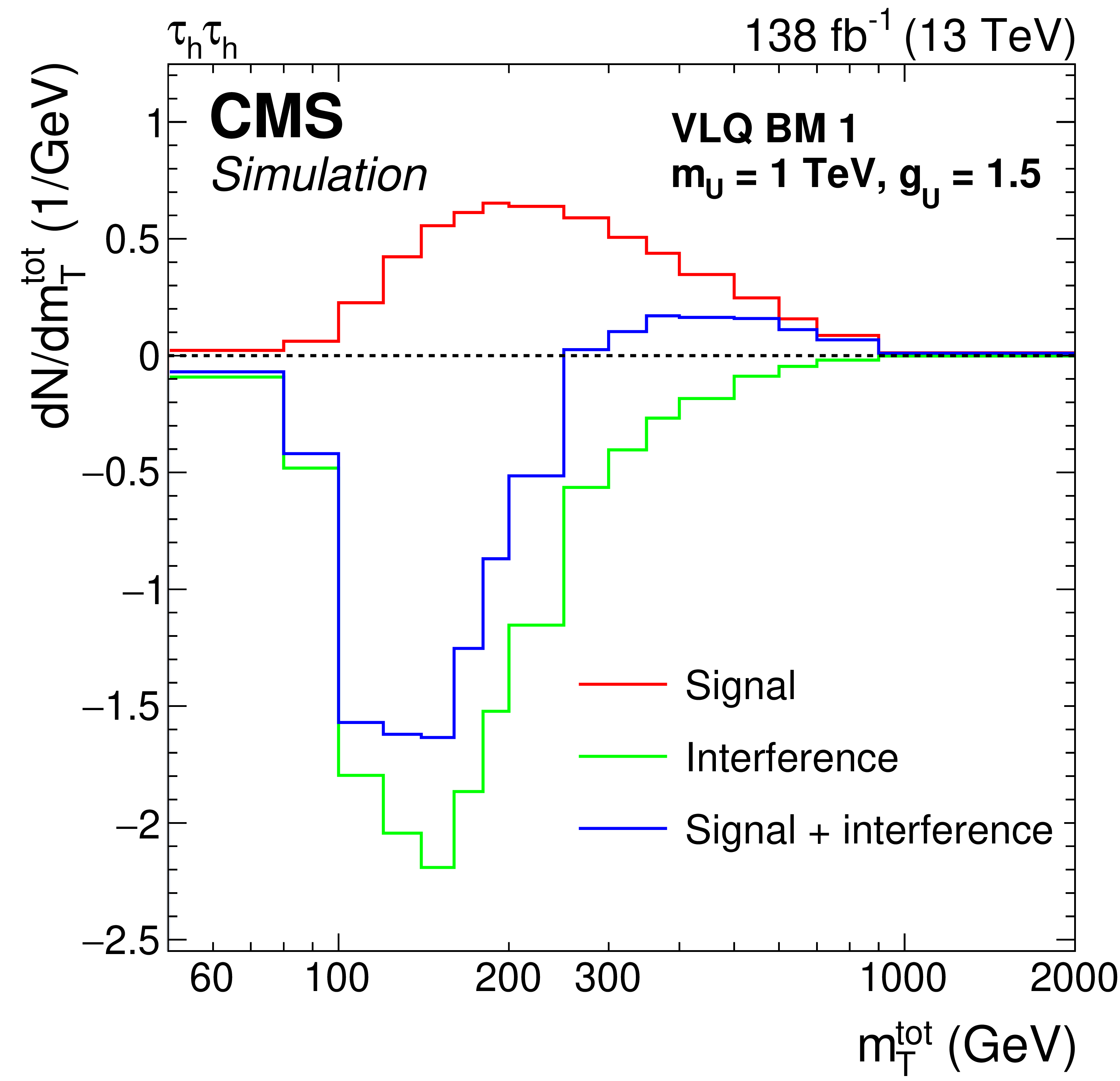
Composition of the signal for the MSSM interpretation of the data and the vector leptoquark search. The left figure shows the generator level A boson ${p_{\mathrm {T}}}$ density for the MSSM ${M_{\mathrm {h}}^{125}}$ scenario for $ {m_{{\mathrm {A}}}} = $ 1.6 TeV and $ {\tan\beta} =$ 30, split by the contributions from the t quark only, the b quark only, and the tb-interference term. The right figure shows the distribution of ${m_{\mathrm {T}}^{\text {tot}}}$ at reconstruction level in the ${{\tau _\mathrm {h}} {\tau _\mathrm {h}}}$ final state for U$_{1}$ $t$-channel exchange with $ {m_{\text {U}}} = $ 1 TeV and $ {g_{\text {U}}} =$ 1.5, for the signal with and without the interference term for the VLQ BM 1 scenario. The ${{\tau _\mathrm {h}} {\tau _\mathrm {h}}}$ final state is shown, since it is the most sensitive one for this search. The bins of the distributions are divided by their width and the distribution is normalized to the expected signal yield for 138 fb$^{-1}$. |
png pdf |
Figure 7-a:
Composition of the signal for the MSSM interpretation of the data and the vector leptoquark search. The left figure shows the generator level A boson ${p_{\mathrm {T}}}$ density for the MSSM ${M_{\mathrm {h}}^{125}}$ scenario for $ {m_{{\mathrm {A}}}} = $ 1.6 TeV and $ {\tan\beta} =$ 30, split by the contributions from the t quark only, the b quark only, and the tb-interference term. The right figure shows the distribution of ${m_{\mathrm {T}}^{\text {tot}}}$ at reconstruction level in the ${{\tau _\mathrm {h}} {\tau _\mathrm {h}}}$ final state for U$_{1}$ $t$-channel exchange with $ {m_{\text {U}}} = $ 1 TeV and $ {g_{\text {U}}} =$ 1.5, for the signal with and without the interference term for the VLQ BM 1 scenario. The ${{\tau _\mathrm {h}} {\tau _\mathrm {h}}}$ final state is shown, since it is the most sensitive one for this search. The bins of the distributions are divided by their width and the distribution is normalized to the expected signal yield for 138 fb$^{-1}$. |
png pdf |
Figure 7-b:
Composition of the signal for the MSSM interpretation of the data and the vector leptoquark search. The left figure shows the generator level A boson ${p_{\mathrm {T}}}$ density for the MSSM ${M_{\mathrm {h}}^{125}}$ scenario for $ {m_{{\mathrm {A}}}} = $ 1.6 TeV and $ {\tan\beta} =$ 30, split by the contributions from the t quark only, the b quark only, and the tb-interference term. The right figure shows the distribution of ${m_{\mathrm {T}}^{\text {tot}}}$ at reconstruction level in the ${{\tau _\mathrm {h}} {\tau _\mathrm {h}}}$ final state for U$_{1}$ $t$-channel exchange with $ {m_{\text {U}}} = $ 1 TeV and $ {g_{\text {U}}} =$ 1.5, for the signal with and without the interference term for the VLQ BM 1 scenario. The ${{\tau _\mathrm {h}} {\tau _\mathrm {h}}}$ final state is shown, since it is the most sensitive one for this search. The bins of the distributions are divided by their width and the distribution is normalized to the expected signal yield for 138 fb$^{-1}$. |

png pdf |
Figure 8:
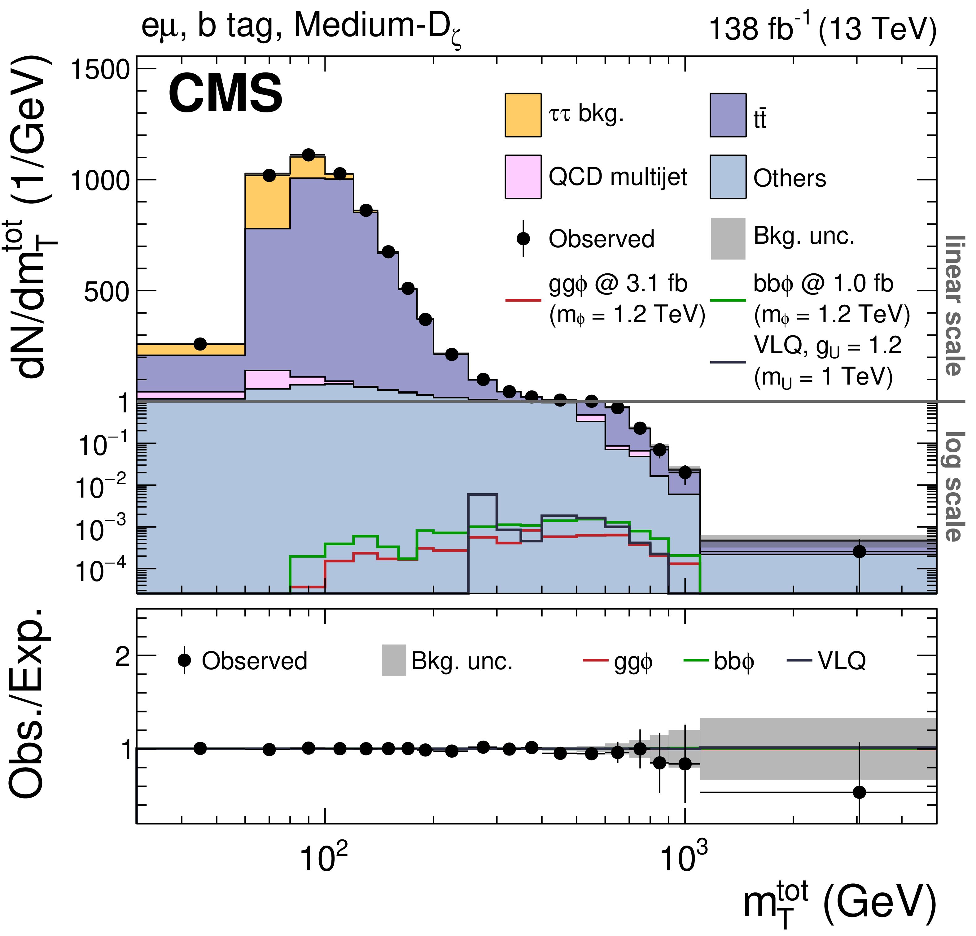
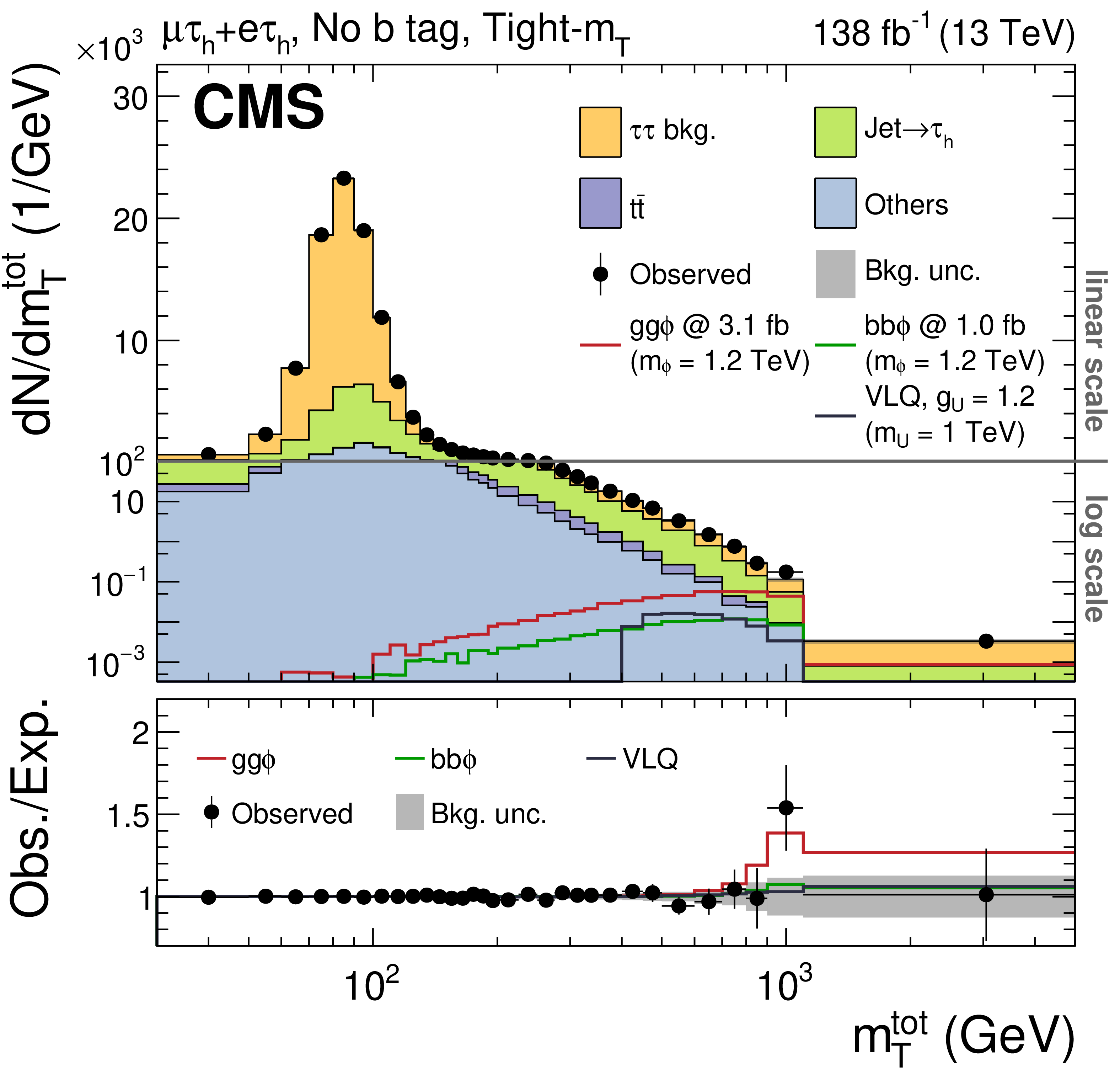
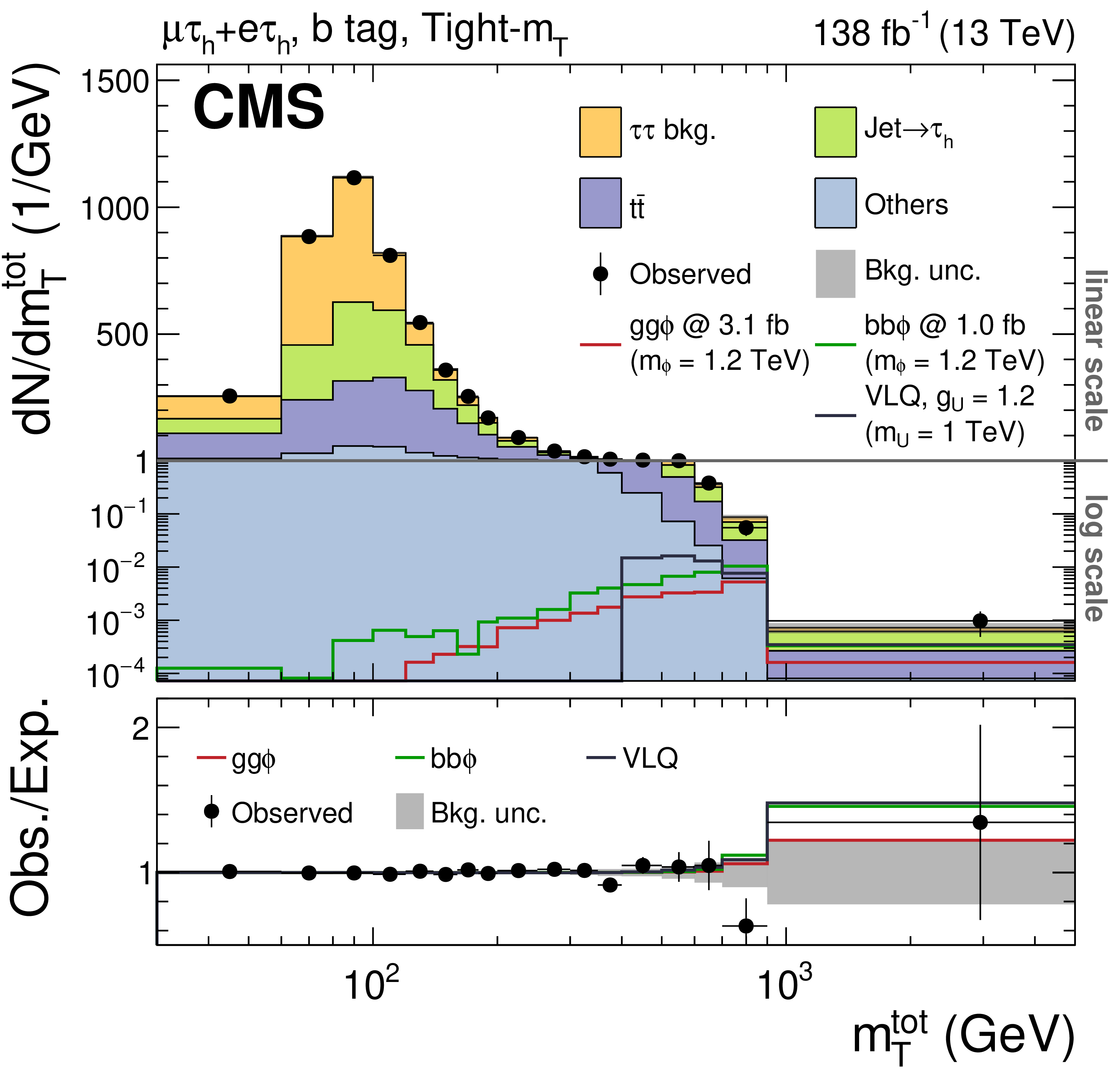
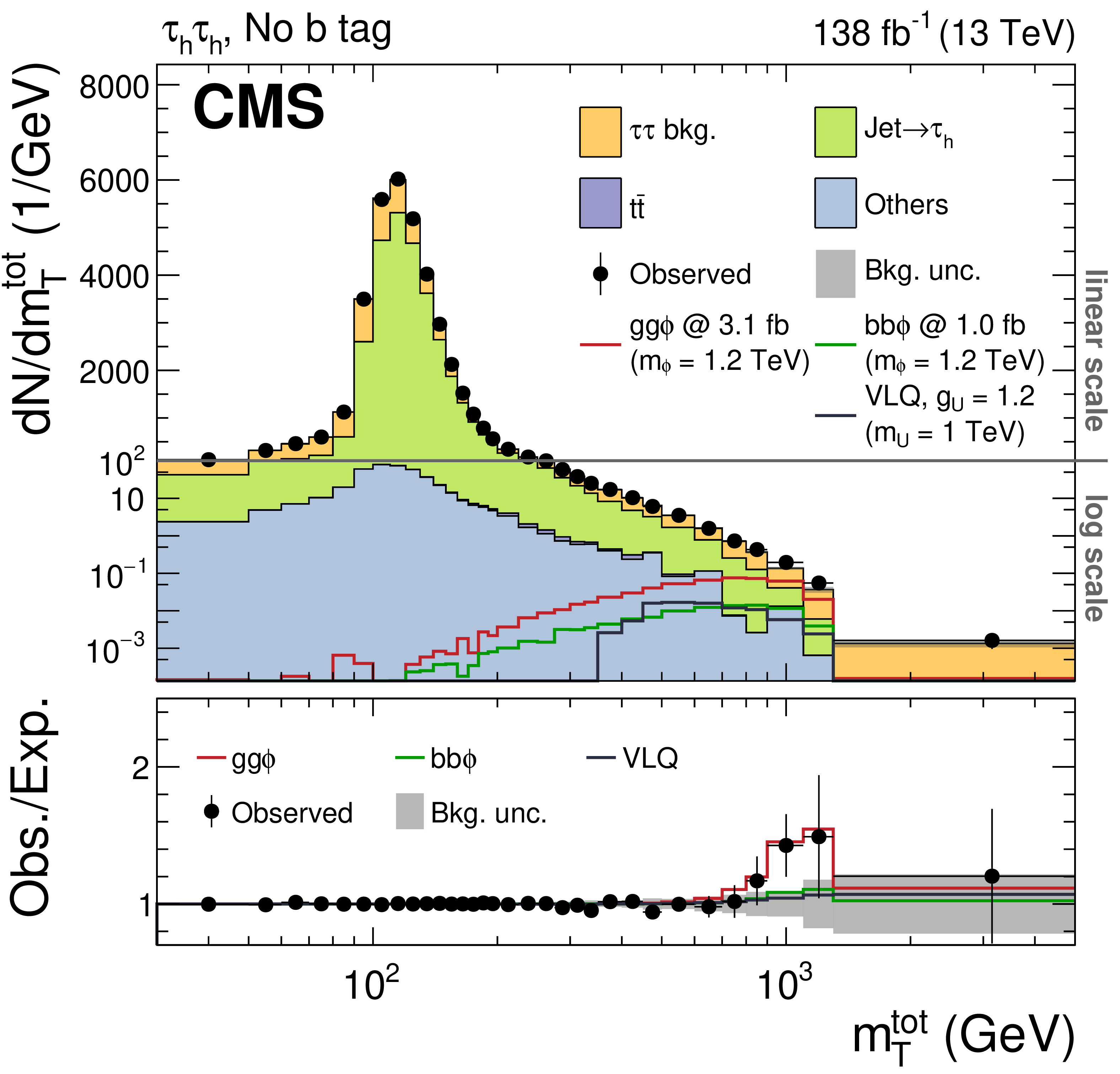
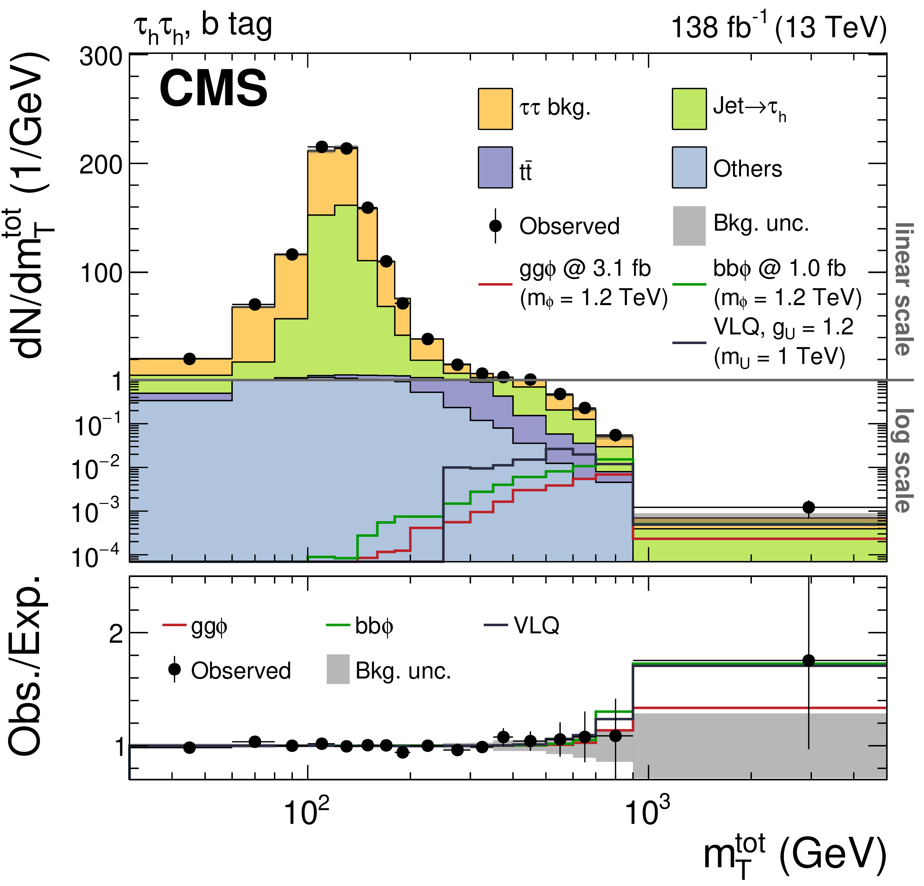
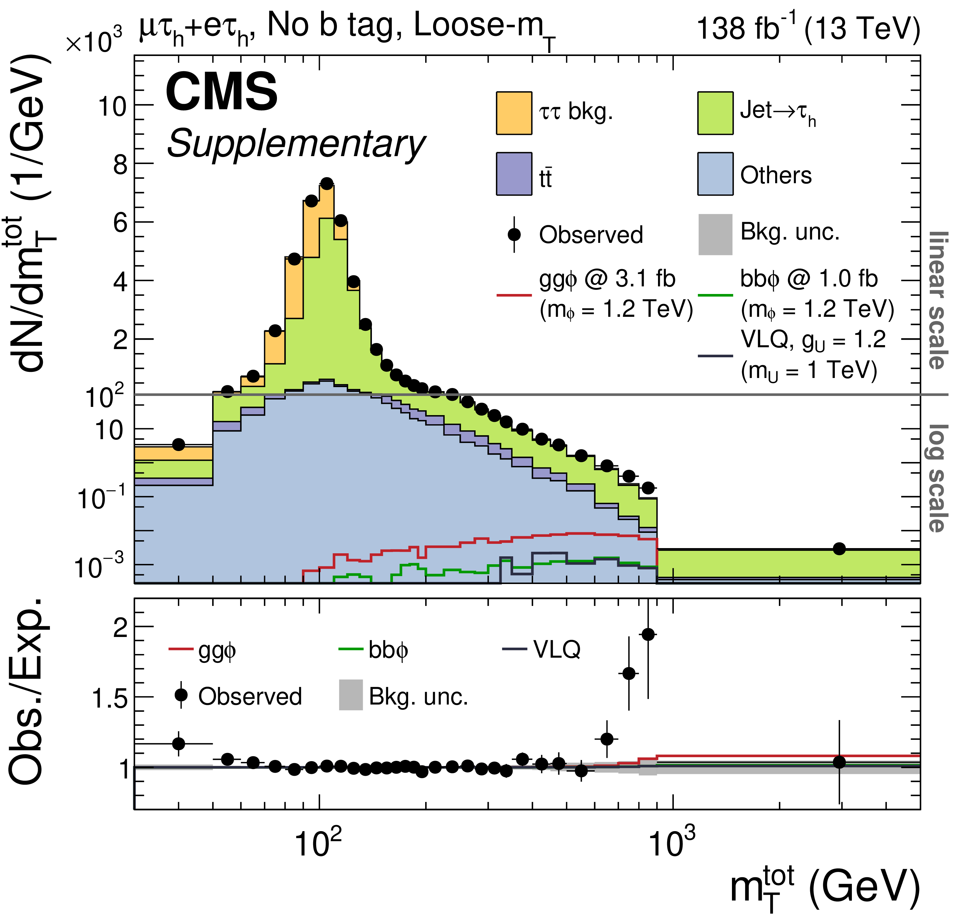
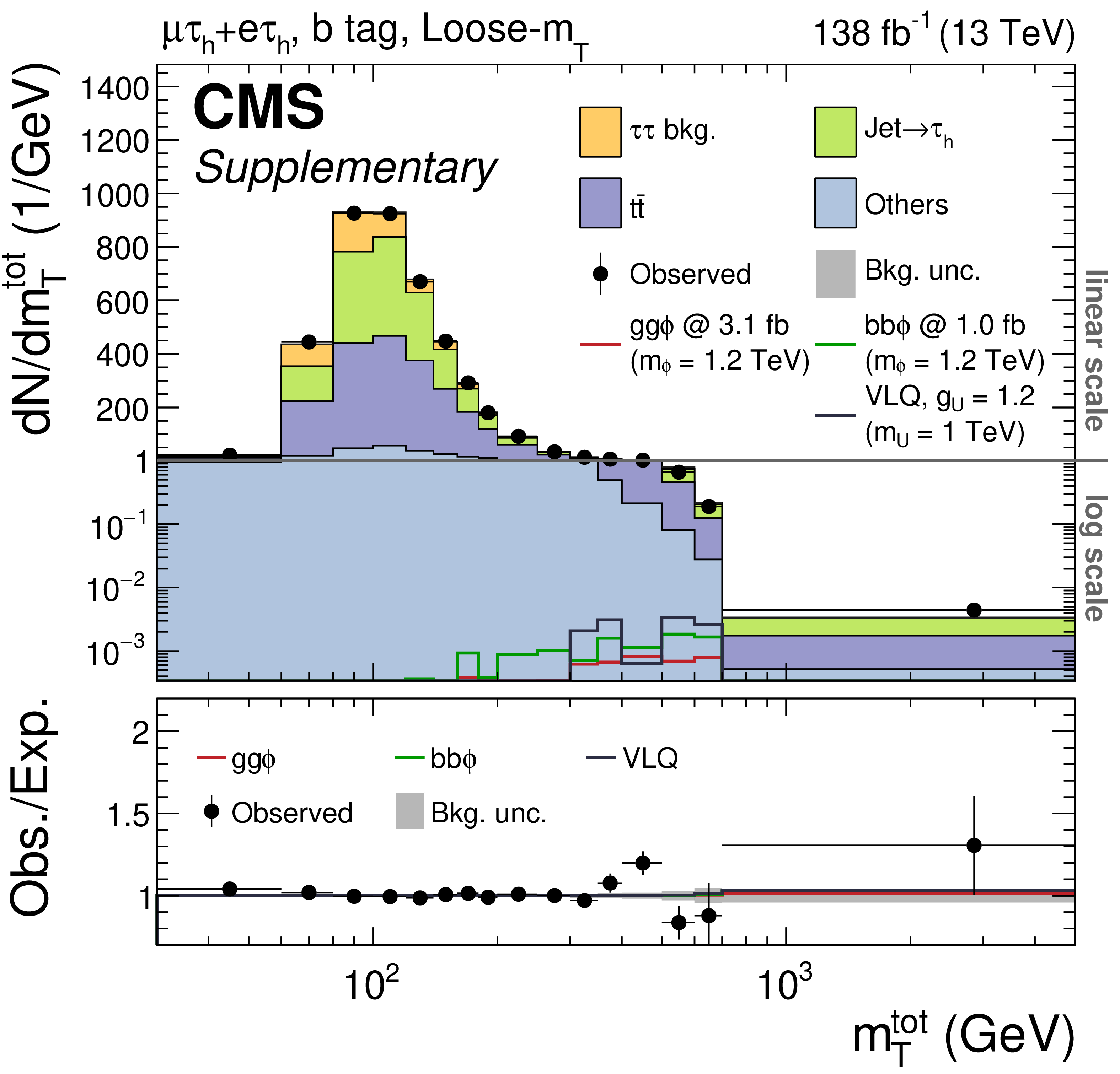
Distributions of ${m_{\mathrm {T}}^{\text {tot}}}$ in the global (left) "no b tag'' and (right) "b tag'' categories in the (upper) e$\mu$, (middle) e$ {\tau _\mathrm {h}}$ and $\mu {\tau _\mathrm {h}}$, and (lower) ${{\tau _\mathrm {h}} {\tau _\mathrm {h}}}$ final states. For the e$\mu$ final state, the medium-D$_{\zeta}$ category is displayed; for the e$ {\tau _\mathrm {h}}$ and $\mu {\tau _\mathrm {h}}$ final states the tight-${m_{\mathrm {T}}}$ categories are shown. The solid histograms show the stacked background predictions after a signal-plus-background fit to the data for $ {m_{\phi}} = $ 1.2 TeV. The best fit gg$\phi$ signal is shown by the red line. The bb$\phi$ and U$_{1}$ signals are also shown for illustrative purposes. For all histograms, the bin contents show the event yields divided by the bin widths. The lower panel shows the ratio of the data to the background expectation after the signal-plus-background fit to the data. |

png pdf |
Figure 8-a:
Distributions of ${m_{\mathrm {T}}^{\text {tot}}}$ in the global (left) "no b tag'' and (right) "b tag'' categories in the (upper) e$\mu$, (middle) e$ {\tau _\mathrm {h}}$ and $\mu {\tau _\mathrm {h}}$, and (lower) ${{\tau _\mathrm {h}} {\tau _\mathrm {h}}}$ final states. For the e$\mu$ final state, the medium-D$_{\zeta}$ category is displayed; for the e$ {\tau _\mathrm {h}}$ and $\mu {\tau _\mathrm {h}}$ final states the tight-${m_{\mathrm {T}}}$ categories are shown. The solid histograms show the stacked background predictions after a signal-plus-background fit to the data for $ {m_{\phi}} = $ 1.2 TeV. The best fit gg$\phi$ signal is shown by the red line. The bb$\phi$ and U$_{1}$ signals are also shown for illustrative purposes. For all histograms, the bin contents show the event yields divided by the bin widths. The lower panel shows the ratio of the data to the background expectation after the signal-plus-background fit to the data. |
png pdf |
Figure 8-b:
Distributions of ${m_{\mathrm {T}}^{\text {tot}}}$ in the global (left) "no b tag'' and (right) "b tag'' categories in the (upper) e$\mu$, (middle) e$ {\tau _\mathrm {h}}$ and $\mu {\tau _\mathrm {h}}$, and (lower) ${{\tau _\mathrm {h}} {\tau _\mathrm {h}}}$ final states. For the e$\mu$ final state, the medium-D$_{\zeta}$ category is displayed; for the e$ {\tau _\mathrm {h}}$ and $\mu {\tau _\mathrm {h}}$ final states the tight-${m_{\mathrm {T}}}$ categories are shown. The solid histograms show the stacked background predictions after a signal-plus-background fit to the data for $ {m_{\phi}} = $ 1.2 TeV. The best fit gg$\phi$ signal is shown by the red line. The bb$\phi$ and U$_{1}$ signals are also shown for illustrative purposes. For all histograms, the bin contents show the event yields divided by the bin widths. The lower panel shows the ratio of the data to the background expectation after the signal-plus-background fit to the data. |
png pdf |
Figure 8-c:
Distributions of ${m_{\mathrm {T}}^{\text {tot}}}$ in the global (left) "no b tag'' and (right) "b tag'' categories in the (upper) e$\mu$, (middle) e$ {\tau _\mathrm {h}}$ and $\mu {\tau _\mathrm {h}}$, and (lower) ${{\tau _\mathrm {h}} {\tau _\mathrm {h}}}$ final states. For the e$\mu$ final state, the medium-D$_{\zeta}$ category is displayed; for the e$ {\tau _\mathrm {h}}$ and $\mu {\tau _\mathrm {h}}$ final states the tight-${m_{\mathrm {T}}}$ categories are shown. The solid histograms show the stacked background predictions after a signal-plus-background fit to the data for $ {m_{\phi}} = $ 1.2 TeV. The best fit gg$\phi$ signal is shown by the red line. The bb$\phi$ and U$_{1}$ signals are also shown for illustrative purposes. For all histograms, the bin contents show the event yields divided by the bin widths. The lower panel shows the ratio of the data to the background expectation after the signal-plus-background fit to the data. |
png pdf |
Figure 8-d:
Distributions of ${m_{\mathrm {T}}^{\text {tot}}}$ in the global (left) "no b tag'' and (right) "b tag'' categories in the (upper) e$\mu$, (middle) e$ {\tau _\mathrm {h}}$ and $\mu {\tau _\mathrm {h}}$, and (lower) ${{\tau _\mathrm {h}} {\tau _\mathrm {h}}}$ final states. For the e$\mu$ final state, the medium-D$_{\zeta}$ category is displayed; for the e$ {\tau _\mathrm {h}}$ and $\mu {\tau _\mathrm {h}}$ final states the tight-${m_{\mathrm {T}}}$ categories are shown. The solid histograms show the stacked background predictions after a signal-plus-background fit to the data for $ {m_{\phi}} = $ 1.2 TeV. The best fit gg$\phi$ signal is shown by the red line. The bb$\phi$ and U$_{1}$ signals are also shown for illustrative purposes. For all histograms, the bin contents show the event yields divided by the bin widths. The lower panel shows the ratio of the data to the background expectation after the signal-plus-background fit to the data. |
png pdf |
Figure 8-e:
Distributions of ${m_{\mathrm {T}}^{\text {tot}}}$ in the global (left) "no b tag'' and (right) "b tag'' categories in the (upper) e$\mu$, (middle) e$ {\tau _\mathrm {h}}$ and $\mu {\tau _\mathrm {h}}$, and (lower) ${{\tau _\mathrm {h}} {\tau _\mathrm {h}}}$ final states. For the e$\mu$ final state, the medium-D$_{\zeta}$ category is displayed; for the e$ {\tau _\mathrm {h}}$ and $\mu {\tau _\mathrm {h}}$ final states the tight-${m_{\mathrm {T}}}$ categories are shown. The solid histograms show the stacked background predictions after a signal-plus-background fit to the data for $ {m_{\phi}} = $ 1.2 TeV. The best fit gg$\phi$ signal is shown by the red line. The bb$\phi$ and U$_{1}$ signals are also shown for illustrative purposes. For all histograms, the bin contents show the event yields divided by the bin widths. The lower panel shows the ratio of the data to the background expectation after the signal-plus-background fit to the data. |
png pdf |
Figure 8-f:
Distributions of ${m_{\mathrm {T}}^{\text {tot}}}$ in the global (left) "no b tag'' and (right) "b tag'' categories in the (upper) e$\mu$, (middle) e$ {\tau _\mathrm {h}}$ and $\mu {\tau _\mathrm {h}}$, and (lower) ${{\tau _\mathrm {h}} {\tau _\mathrm {h}}}$ final states. For the e$\mu$ final state, the medium-D$_{\zeta}$ category is displayed; for the e$ {\tau _\mathrm {h}}$ and $\mu {\tau _\mathrm {h}}$ final states the tight-${m_{\mathrm {T}}}$ categories are shown. The solid histograms show the stacked background predictions after a signal-plus-background fit to the data for $ {m_{\phi}} = $ 1.2 TeV. The best fit gg$\phi$ signal is shown by the red line. The bb$\phi$ and U$_{1}$ signals are also shown for illustrative purposes. For all histograms, the bin contents show the event yields divided by the bin widths. The lower panel shows the ratio of the data to the background expectation after the signal-plus-background fit to the data. |
png pdf |
Figure 9:
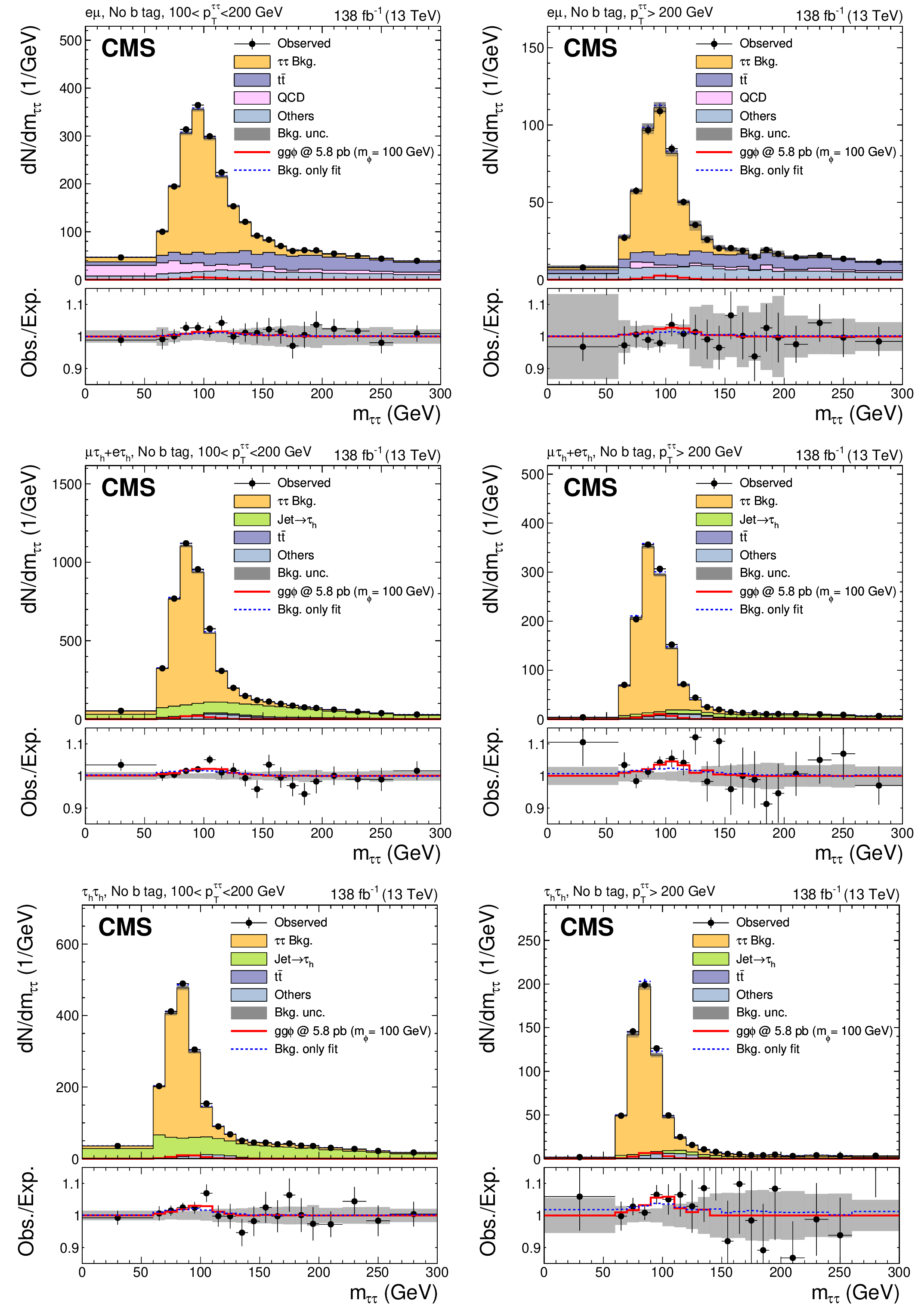
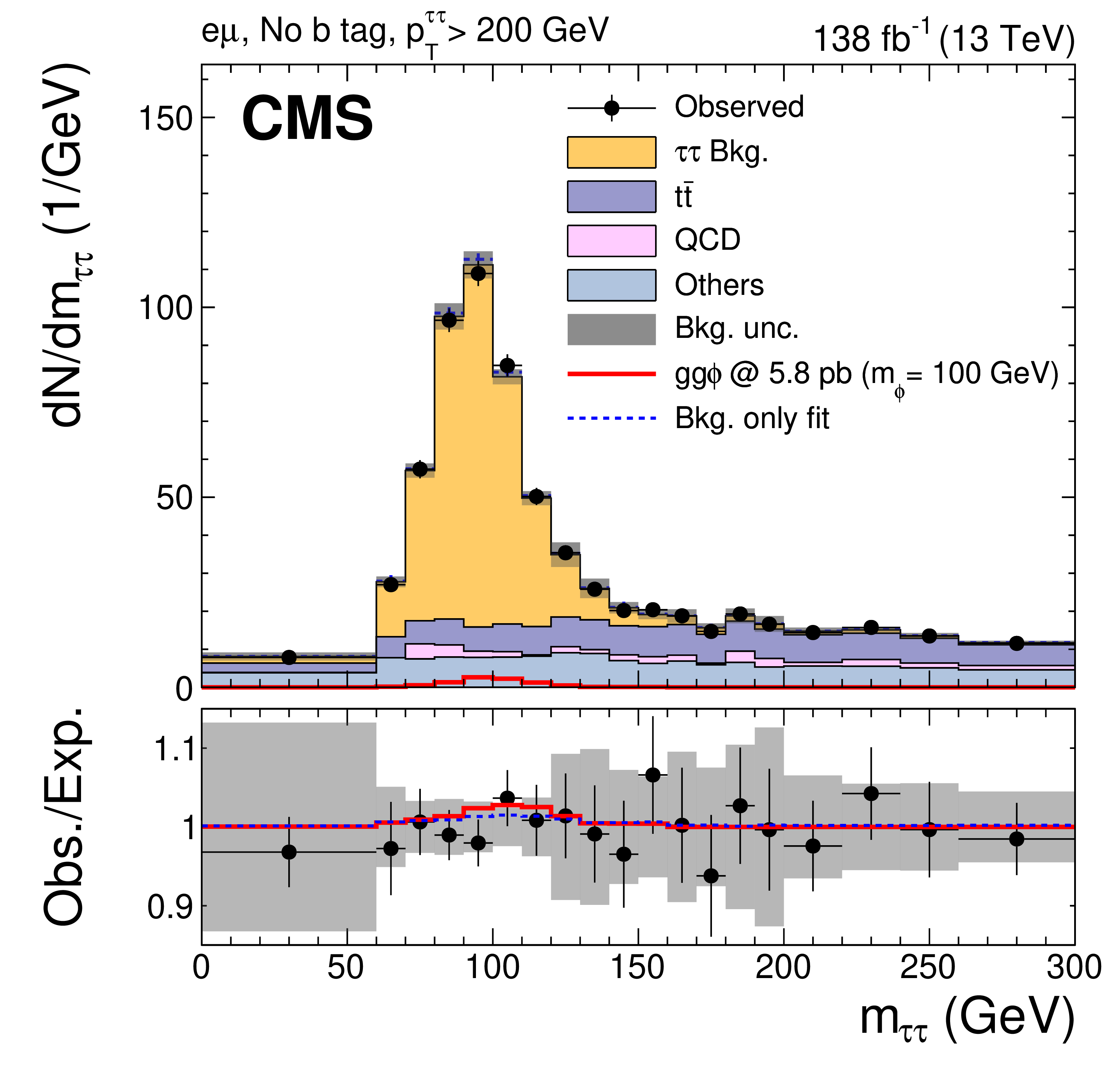
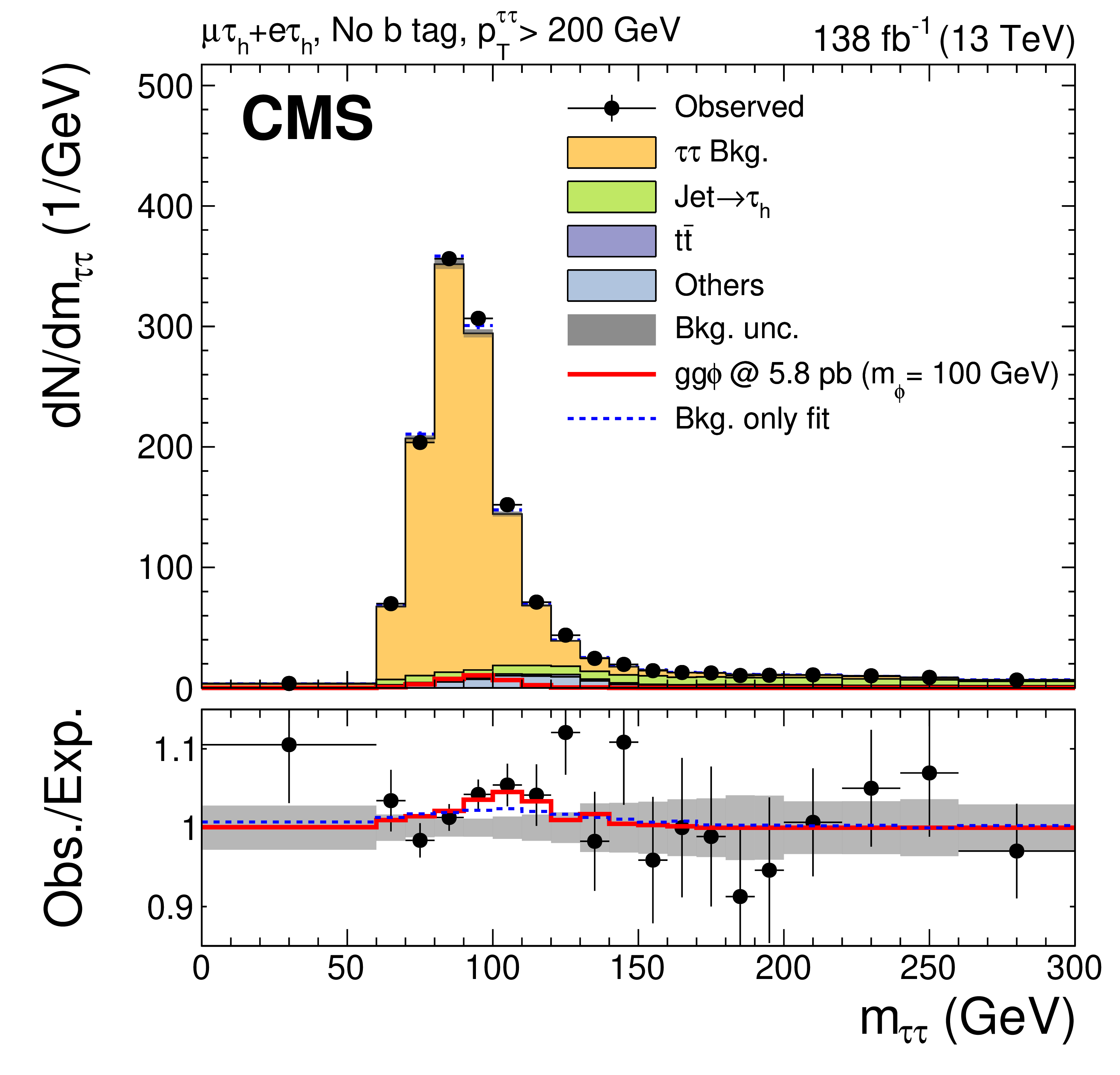
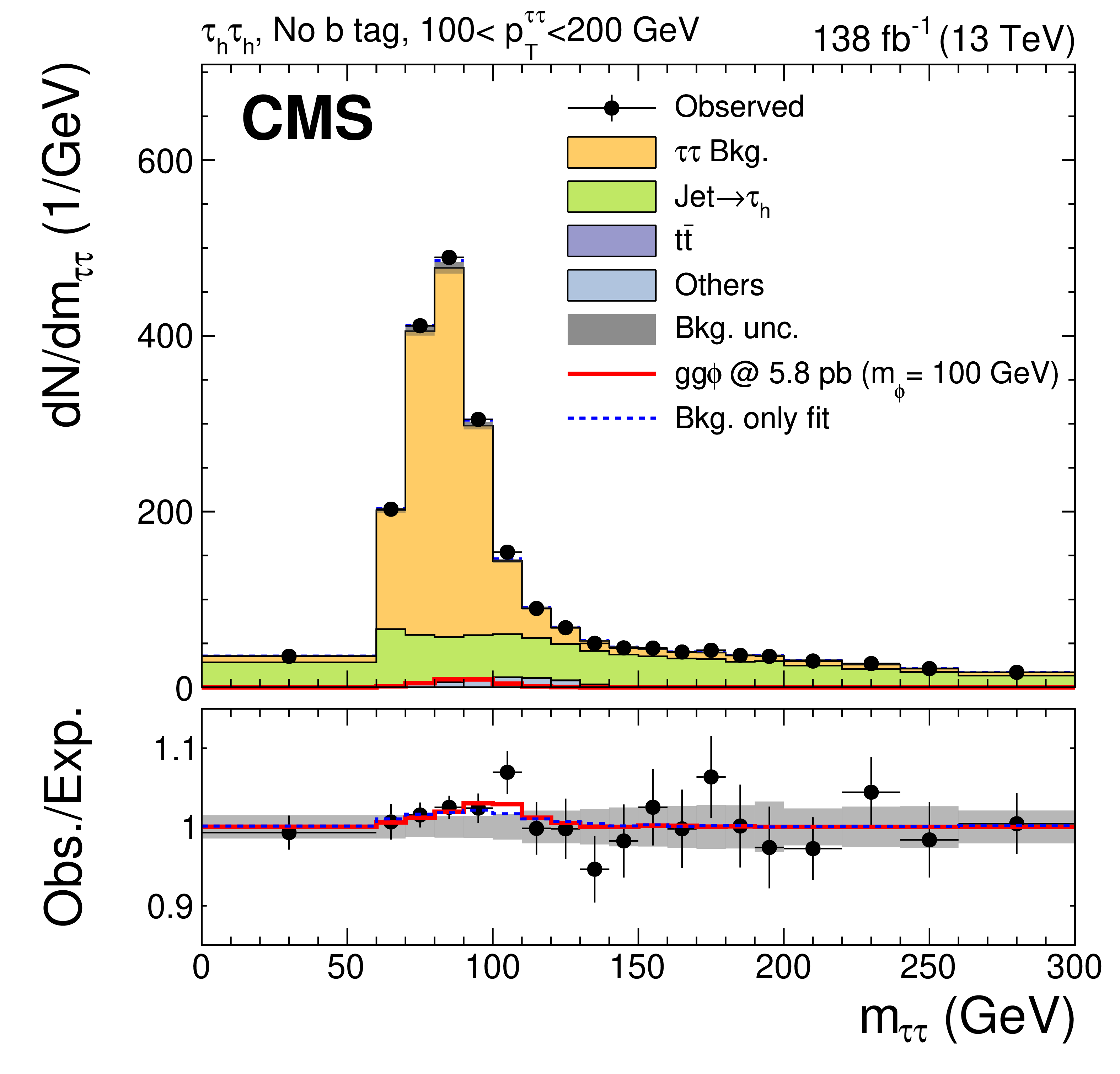
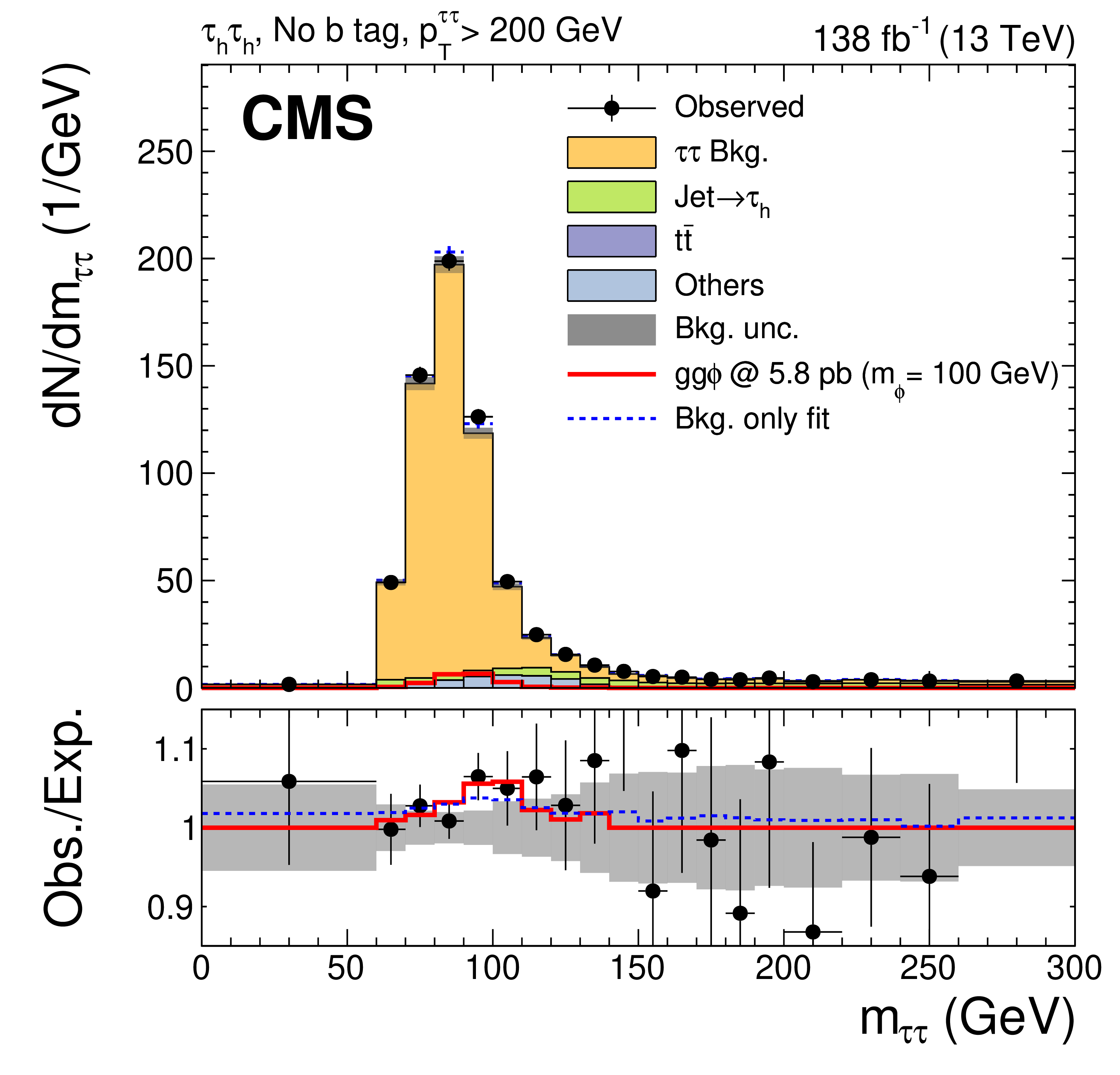
Distributions of ${m_{\tau \tau}}$ in the (left) 100 $ < {{p_{\mathrm {T}}} ^{{\tau \tau}}} < $ 200 GeV and (right) $ {{p_{\mathrm {T}}} ^{{\tau \tau}}} > $ 200 GeV "no b tag'' categories for the (upper) e$\mu$, (middle) e$ {\tau _\mathrm {h}}$ and $\mu {\tau _\mathrm {h}}$, and (lower) ${{\tau _\mathrm {h}} {\tau _\mathrm {h}}}$ final states. The solid histograms show the stacked background predictions after a signal-plus-background fit to the data for $ {m_{\phi}} = $ 100 GeV. The best fit gg$\phi$ signal is shown by the red line. The total background prediction as estimated from a background-only fit to the data is shown by the dashed blue line for comparison. For all histograms, the bin contents show the event yields divided by the bin widths. The lower panel shows the ratio of the data to the background expectation after the signal-plus-background fit to the data. The signal-plus-background and background-only fit predictions are shown by the solid red and dashed blue lines, respectively, which are also shown relative to the background expectation obtained from the signal-plus-background fit to the data. |

png pdf |
Figure 9-a:
Distributions of ${m_{\tau \tau}}$ in the (left) 100 $ < {{p_{\mathrm {T}}} ^{{\tau \tau}}} < $ 200 GeV and (right) $ {{p_{\mathrm {T}}} ^{{\tau \tau}}} > $ 200 GeV "no b tag'' categories for the (upper) e$\mu$, (middle) e$ {\tau _\mathrm {h}}$ and $\mu {\tau _\mathrm {h}}$, and (lower) ${{\tau _\mathrm {h}} {\tau _\mathrm {h}}}$ final states. The solid histograms show the stacked background predictions after a signal-plus-background fit to the data for $ {m_{\phi}} = $ 100 GeV. The best fit gg$\phi$ signal is shown by the red line. The total background prediction as estimated from a background-only fit to the data is shown by the dashed blue line for comparison. For all histograms, the bin contents show the event yields divided by the bin widths. The lower panel shows the ratio of the data to the background expectation after the signal-plus-background fit to the data. The signal-plus-background and background-only fit predictions are shown by the solid red and dashed blue lines, respectively, which are also shown relative to the background expectation obtained from the signal-plus-background fit to the data. |
png pdf |
Figure 9-b:
Distributions of ${m_{\tau \tau}}$ in the (left) 100 $ < {{p_{\mathrm {T}}} ^{{\tau \tau}}} < $ 200 GeV and (right) $ {{p_{\mathrm {T}}} ^{{\tau \tau}}} > $ 200 GeV "no b tag'' categories for the (upper) e$\mu$, (middle) e$ {\tau _\mathrm {h}}$ and $\mu {\tau _\mathrm {h}}$, and (lower) ${{\tau _\mathrm {h}} {\tau _\mathrm {h}}}$ final states. The solid histograms show the stacked background predictions after a signal-plus-background fit to the data for $ {m_{\phi}} = $ 100 GeV. The best fit gg$\phi$ signal is shown by the red line. The total background prediction as estimated from a background-only fit to the data is shown by the dashed blue line for comparison. For all histograms, the bin contents show the event yields divided by the bin widths. The lower panel shows the ratio of the data to the background expectation after the signal-plus-background fit to the data. The signal-plus-background and background-only fit predictions are shown by the solid red and dashed blue lines, respectively, which are also shown relative to the background expectation obtained from the signal-plus-background fit to the data. |
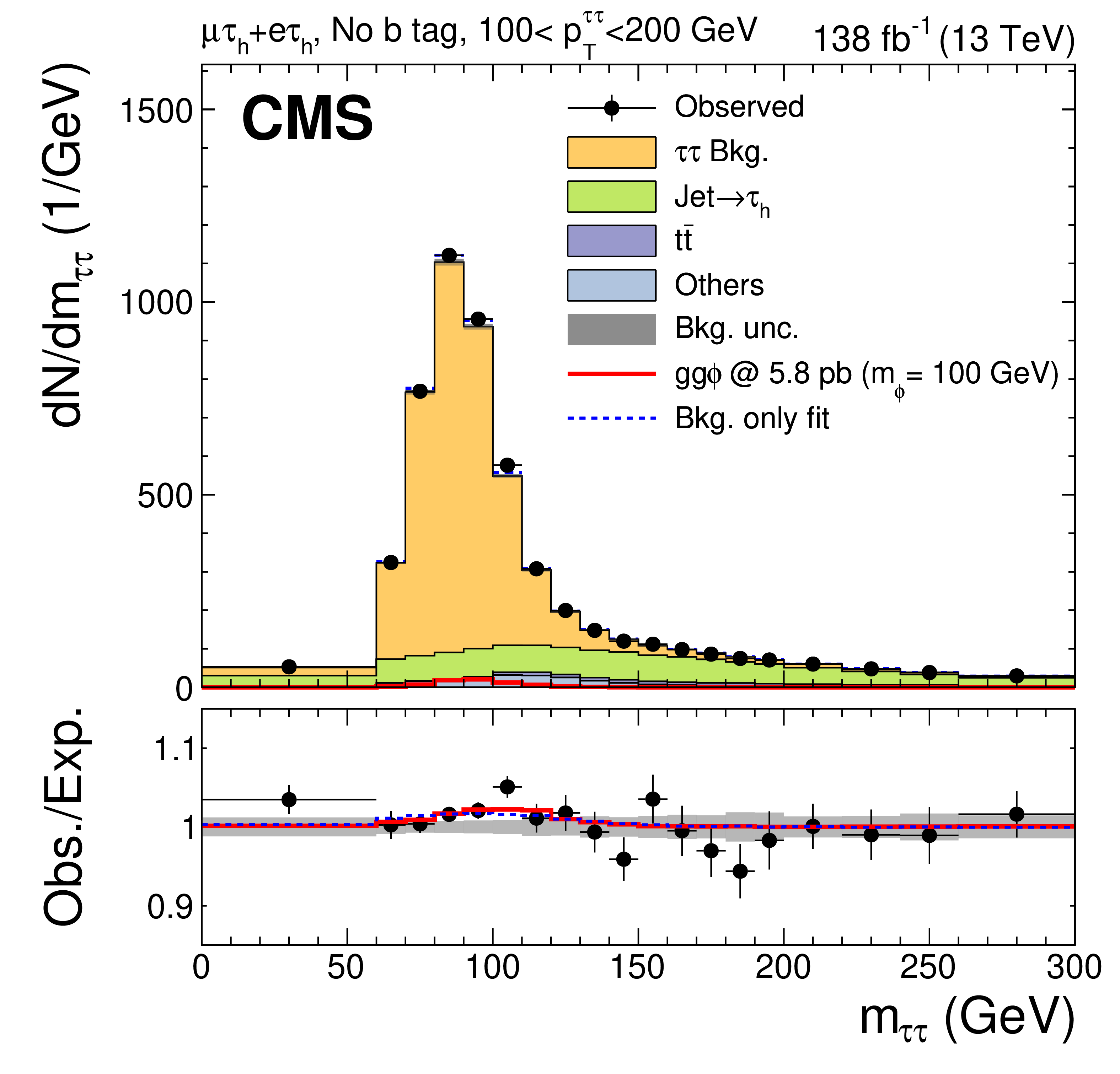
png pdf |
Figure 9-c:
Distributions of ${m_{\tau \tau}}$ in the (left) 100 $ < {{p_{\mathrm {T}}} ^{{\tau \tau}}} < $ 200 GeV and (right) $ {{p_{\mathrm {T}}} ^{{\tau \tau}}} > $ 200 GeV "no b tag'' categories for the (upper) e$\mu$, (middle) e$ {\tau _\mathrm {h}}$ and $\mu {\tau _\mathrm {h}}$, and (lower) ${{\tau _\mathrm {h}} {\tau _\mathrm {h}}}$ final states. The solid histograms show the stacked background predictions after a signal-plus-background fit to the data for $ {m_{\phi}} = $ 100 GeV. The best fit gg$\phi$ signal is shown by the red line. The total background prediction as estimated from a background-only fit to the data is shown by the dashed blue line for comparison. For all histograms, the bin contents show the event yields divided by the bin widths. The lower panel shows the ratio of the data to the background expectation after the signal-plus-background fit to the data. The signal-plus-background and background-only fit predictions are shown by the solid red and dashed blue lines, respectively, which are also shown relative to the background expectation obtained from the signal-plus-background fit to the data. |
png pdf |
Figure 9-d:
Distributions of ${m_{\tau \tau}}$ in the (left) 100 $ < {{p_{\mathrm {T}}} ^{{\tau \tau}}} < $ 200 GeV and (right) $ {{p_{\mathrm {T}}} ^{{\tau \tau}}} > $ 200 GeV "no b tag'' categories for the (upper) e$\mu$, (middle) e$ {\tau _\mathrm {h}}$ and $\mu {\tau _\mathrm {h}}$, and (lower) ${{\tau _\mathrm {h}} {\tau _\mathrm {h}}}$ final states. The solid histograms show the stacked background predictions after a signal-plus-background fit to the data for $ {m_{\phi}} = $ 100 GeV. The best fit gg$\phi$ signal is shown by the red line. The total background prediction as estimated from a background-only fit to the data is shown by the dashed blue line for comparison. For all histograms, the bin contents show the event yields divided by the bin widths. The lower panel shows the ratio of the data to the background expectation after the signal-plus-background fit to the data. The signal-plus-background and background-only fit predictions are shown by the solid red and dashed blue lines, respectively, which are also shown relative to the background expectation obtained from the signal-plus-background fit to the data. |
png pdf |
Figure 9-e:
Distributions of ${m_{\tau \tau}}$ in the (left) 100 $ < {{p_{\mathrm {T}}} ^{{\tau \tau}}} < $ 200 GeV and (right) $ {{p_{\mathrm {T}}} ^{{\tau \tau}}} > $ 200 GeV "no b tag'' categories for the (upper) e$\mu$, (middle) e$ {\tau _\mathrm {h}}$ and $\mu {\tau _\mathrm {h}}$, and (lower) ${{\tau _\mathrm {h}} {\tau _\mathrm {h}}}$ final states. The solid histograms show the stacked background predictions after a signal-plus-background fit to the data for $ {m_{\phi}} = $ 100 GeV. The best fit gg$\phi$ signal is shown by the red line. The total background prediction as estimated from a background-only fit to the data is shown by the dashed blue line for comparison. For all histograms, the bin contents show the event yields divided by the bin widths. The lower panel shows the ratio of the data to the background expectation after the signal-plus-background fit to the data. The signal-plus-background and background-only fit predictions are shown by the solid red and dashed blue lines, respectively, which are also shown relative to the background expectation obtained from the signal-plus-background fit to the data. |
png pdf |
Figure 9-f:
Distributions of ${m_{\tau \tau}}$ in the (left) 100 $ < {{p_{\mathrm {T}}} ^{{\tau \tau}}} < $ 200 GeV and (right) $ {{p_{\mathrm {T}}} ^{{\tau \tau}}} > $ 200 GeV "no b tag'' categories for the (upper) e$\mu$, (middle) e$ {\tau _\mathrm {h}}$ and $\mu {\tau _\mathrm {h}}$, and (lower) ${{\tau _\mathrm {h}} {\tau _\mathrm {h}}}$ final states. The solid histograms show the stacked background predictions after a signal-plus-background fit to the data for $ {m_{\phi}} = $ 100 GeV. The best fit gg$\phi$ signal is shown by the red line. The total background prediction as estimated from a background-only fit to the data is shown by the dashed blue line for comparison. For all histograms, the bin contents show the event yields divided by the bin widths. The lower panel shows the ratio of the data to the background expectation after the signal-plus-background fit to the data. The signal-plus-background and background-only fit predictions are shown by the solid red and dashed blue lines, respectively, which are also shown relative to the background expectation obtained from the signal-plus-background fit to the data. |

png pdf |
Figure 10:
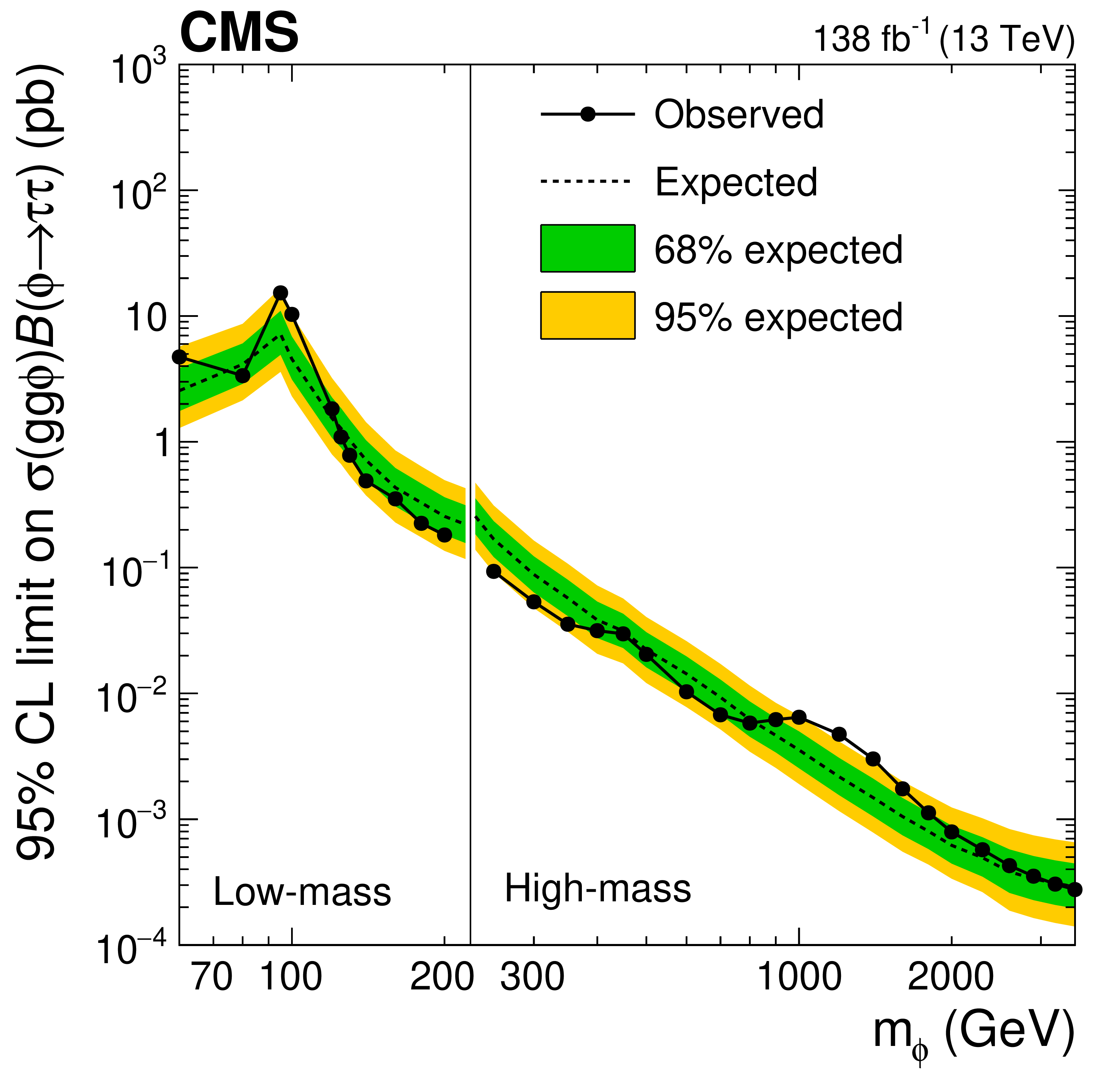
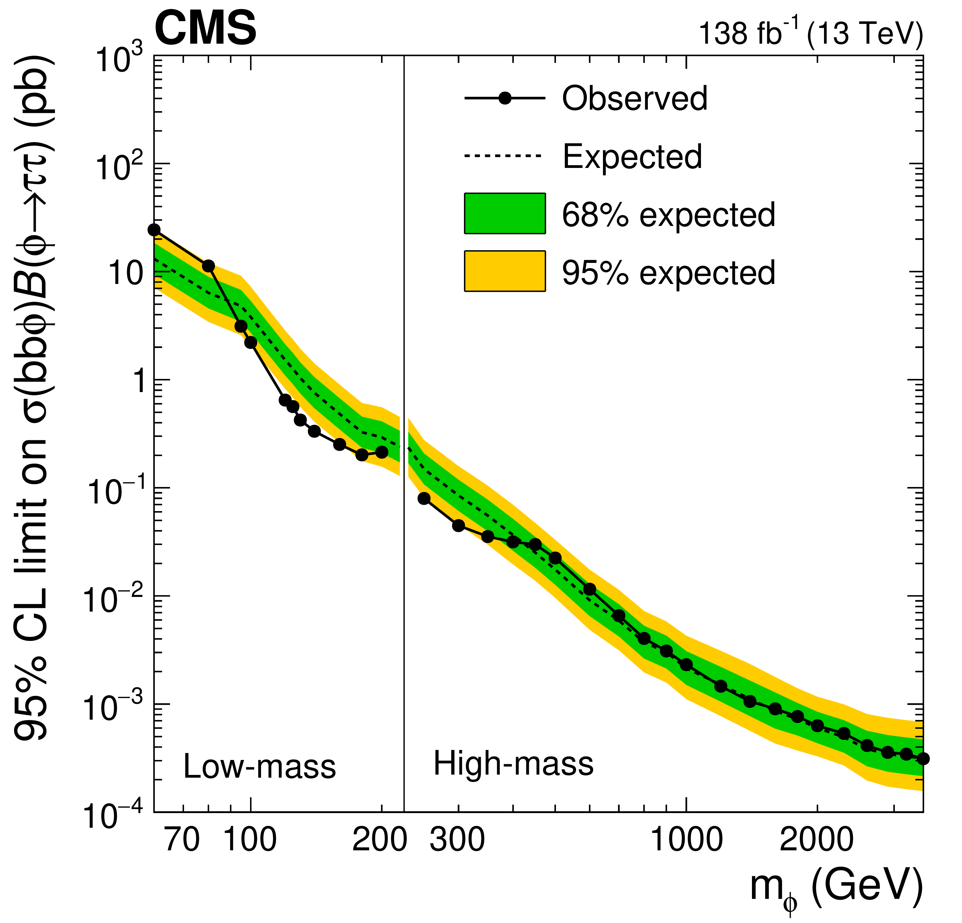
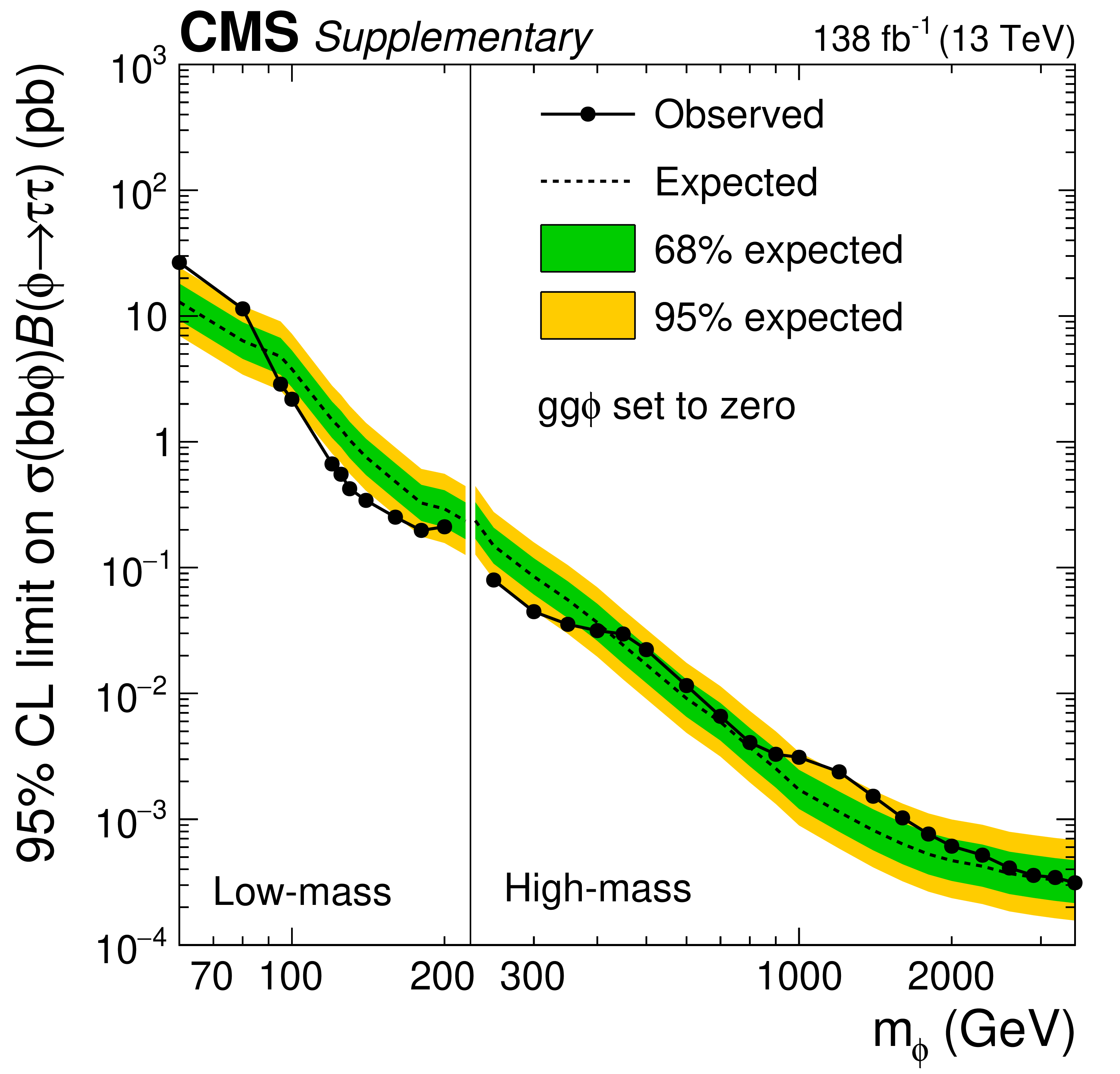
Expected and observed 95% CL upper limits on the product of the cross sections and branching fraction for the decay into $\tau$ leptons for (left) gg$\phi$ and (right) bb$\phi$ production in a mass range of 60 $\leq {m_{\phi}} \leq 3500 GeV $, in addition to H(125). The expected median of the exclusion limit in the absence of signal is shown by the dashed line. The dark green and bright yellow bands indicate the central 68% and 95% intervals for the expected exclusion limit. The black dots correspond to the observed limits. The peak in the expected gg$\phi$ limit emerges from the loss of sensitivity around 90 GeV due to the background from Z/$\gamma$* $\to \tau\tau$ events. |
png pdf |
Figure 10-a:
Expected and observed 95% CL upper limits on the product of the cross sections and branching fraction for the decay into $\tau$ leptons for (left) gg$\phi$ and (right) bb$\phi$ production in a mass range of 60 $\leq {m_{\phi}} \leq 3500 GeV $, in addition to H(125). The expected median of the exclusion limit in the absence of signal is shown by the dashed line. The dark green and bright yellow bands indicate the central 68% and 95% intervals for the expected exclusion limit. The black dots correspond to the observed limits. The peak in the expected gg$\phi$ limit emerges from the loss of sensitivity around 90 GeV due to the background from Z/$\gamma$* $\to \tau\tau$ events. |
png pdf |
Figure 10-b:
Expected and observed 95% CL upper limits on the product of the cross sections and branching fraction for the decay into $\tau$ leptons for (left) gg$\phi$ and (right) bb$\phi$ production in a mass range of 60 $\leq {m_{\phi}} \leq 3500 GeV $, in addition to H(125). The expected median of the exclusion limit in the absence of signal is shown by the dashed line. The dark green and bright yellow bands indicate the central 68% and 95% intervals for the expected exclusion limit. The black dots correspond to the observed limits. The peak in the expected gg$\phi$ limit emerges from the loss of sensitivity around 90 GeV due to the background from Z/$\gamma$* $\to \tau\tau$ events. |
png pdf |
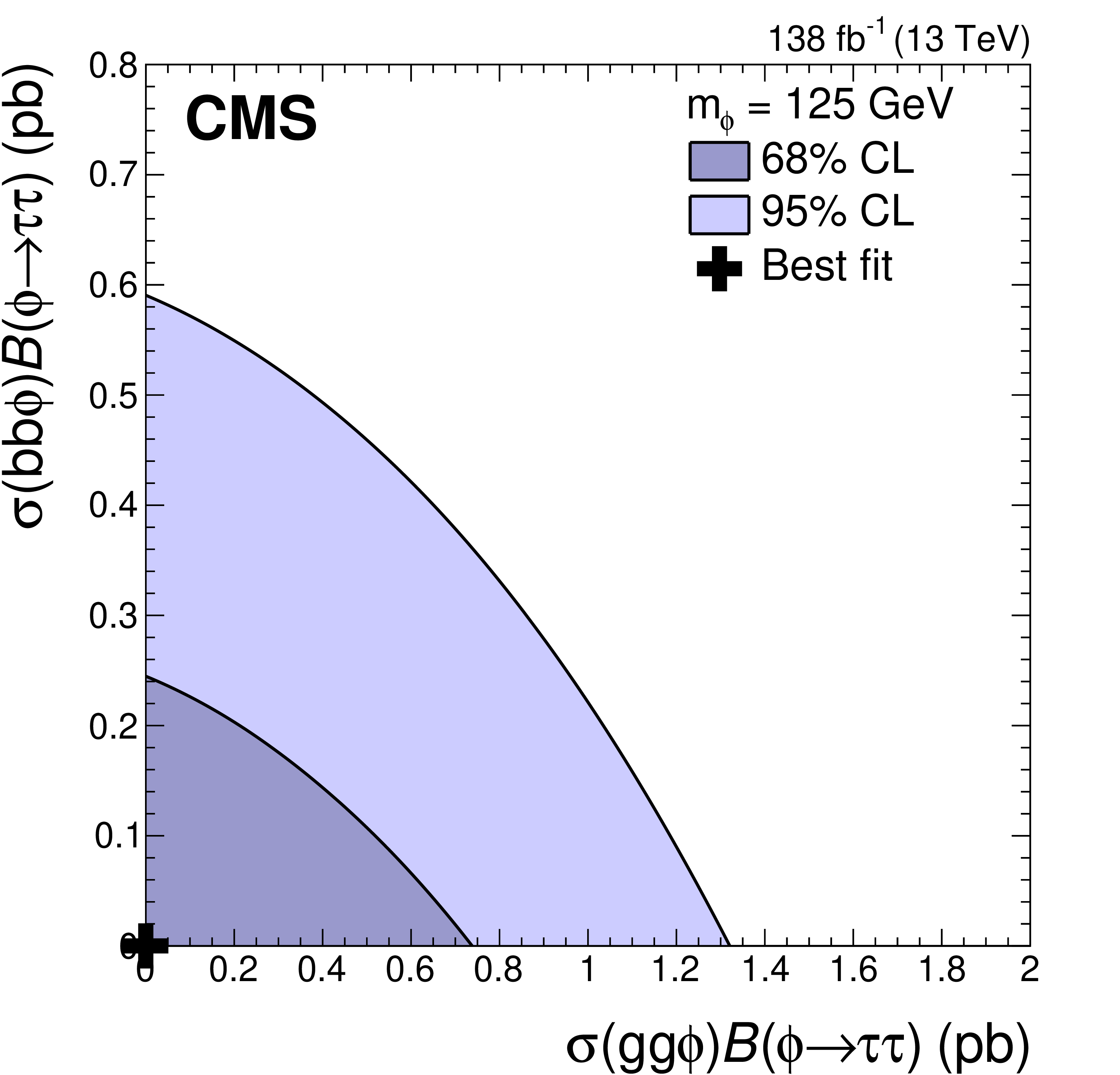
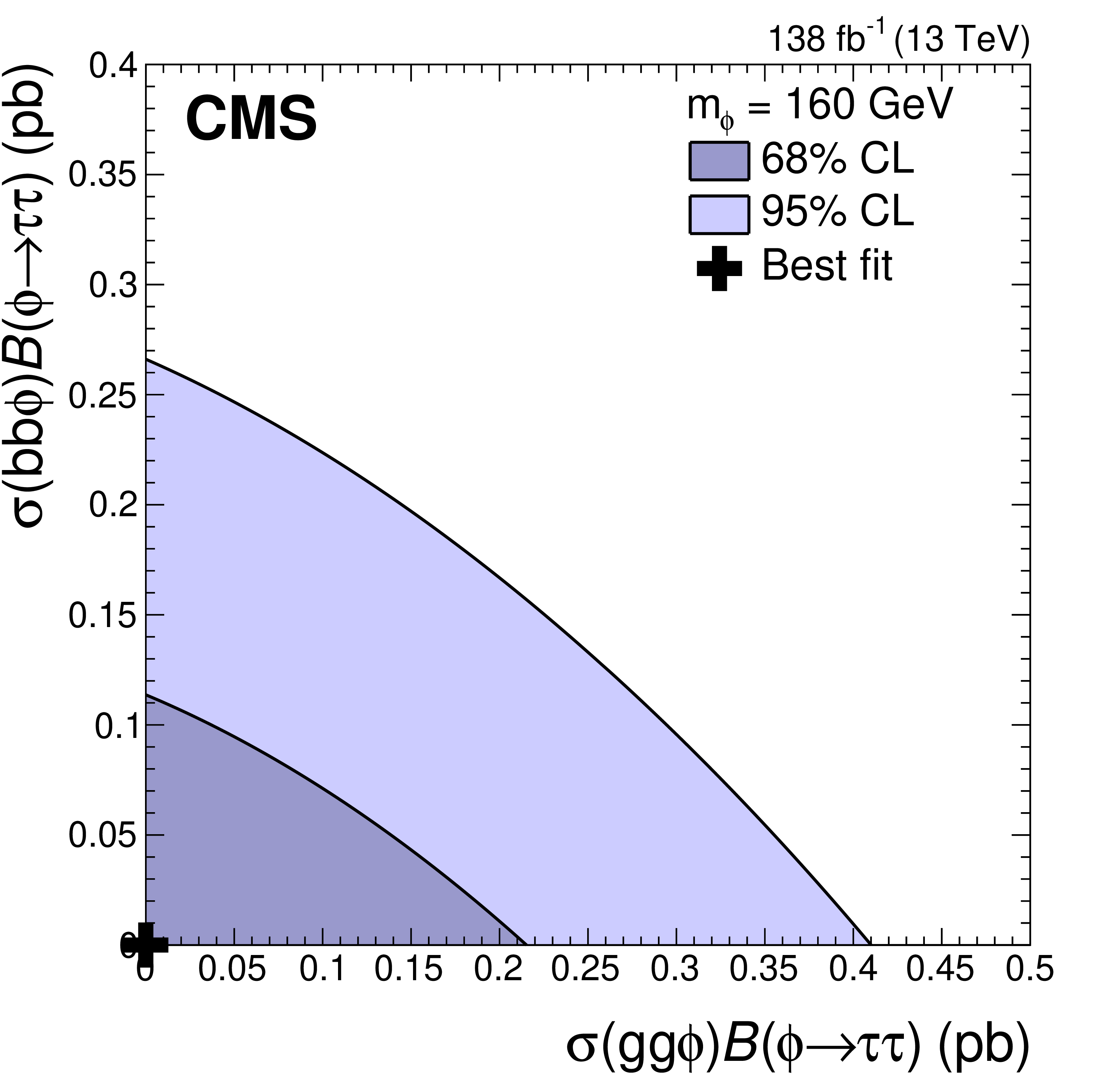
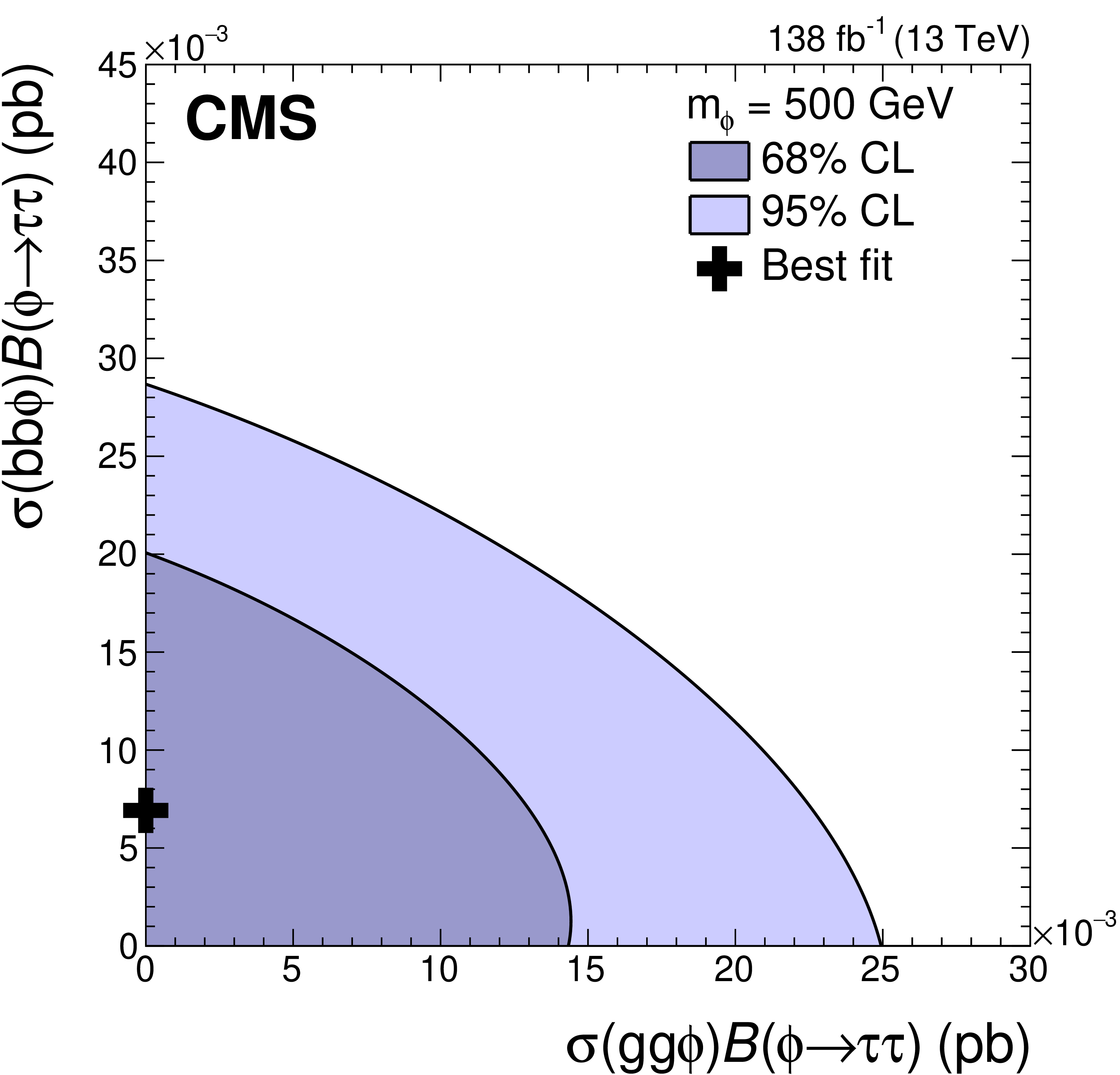
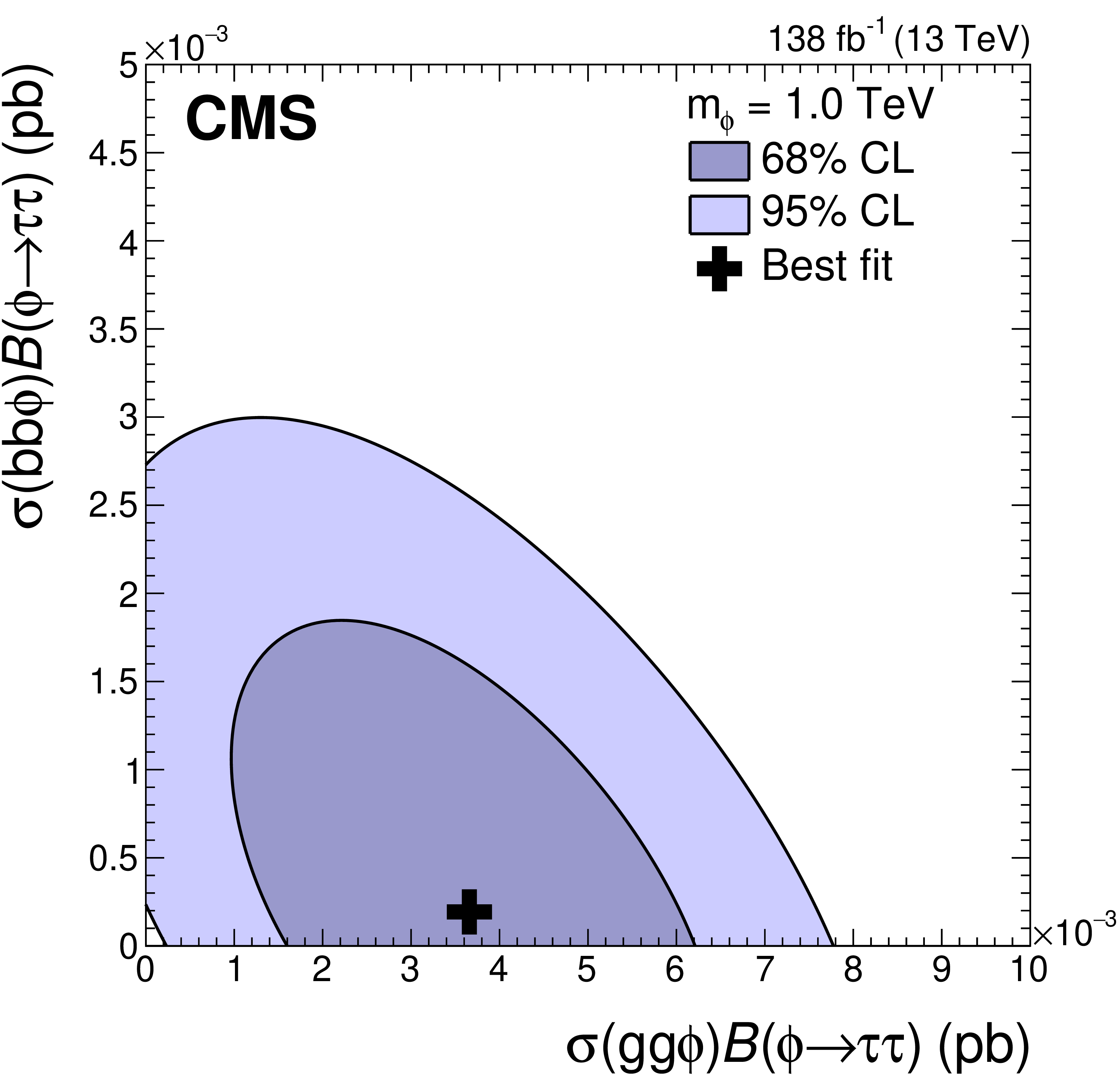
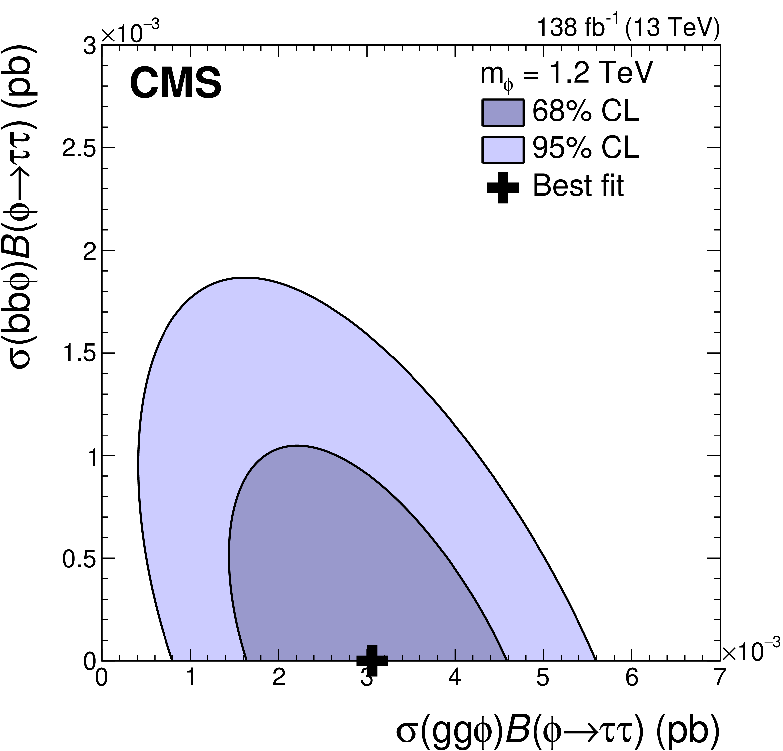
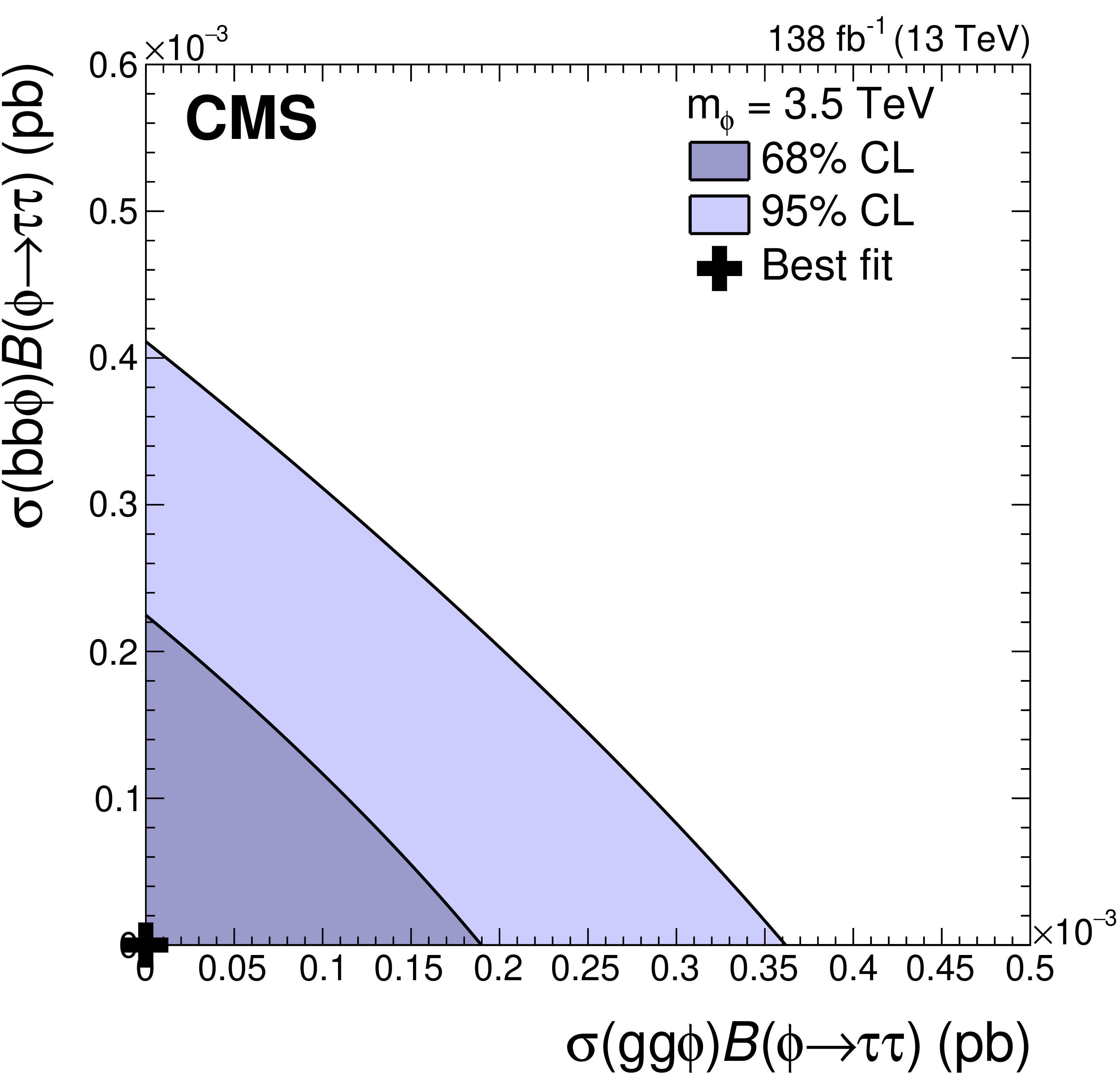
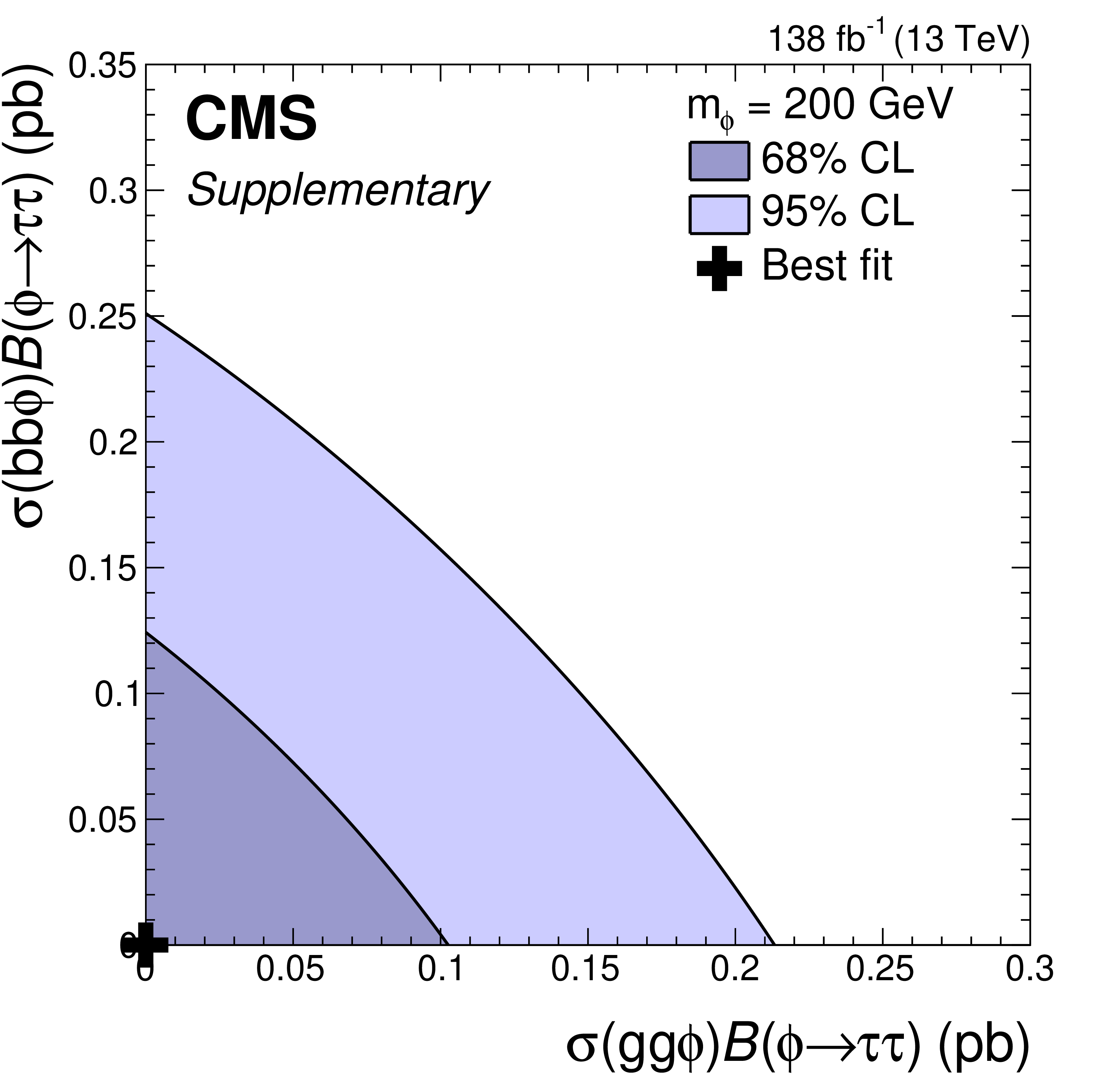
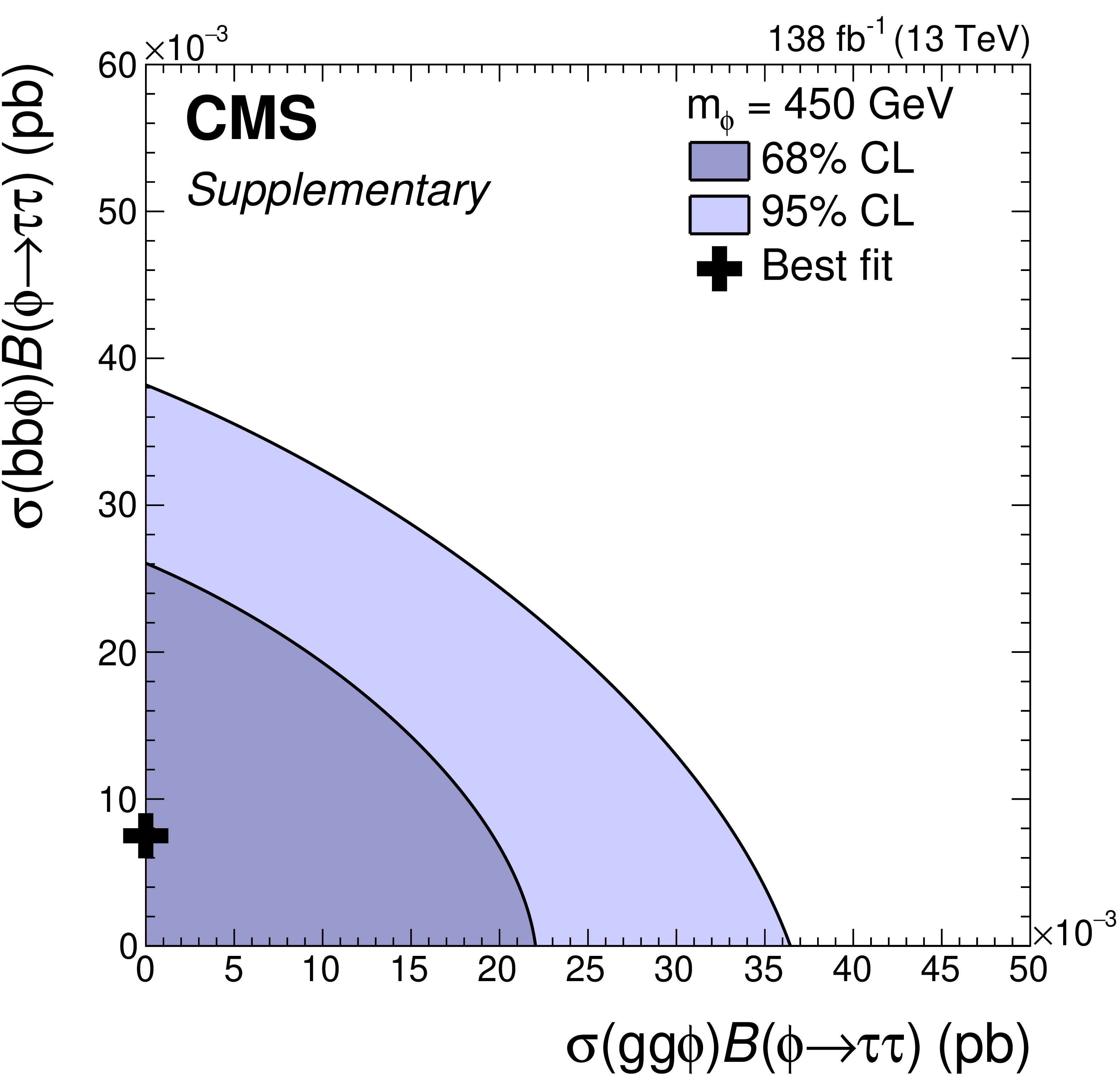
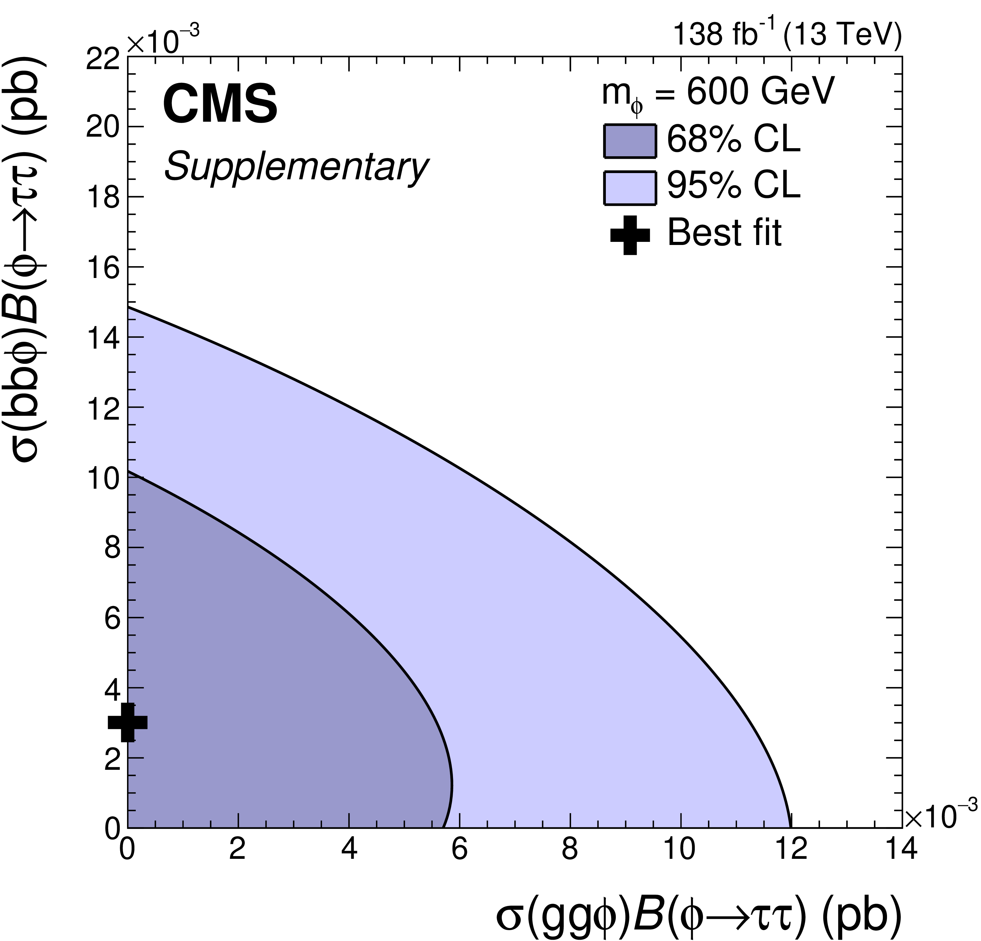
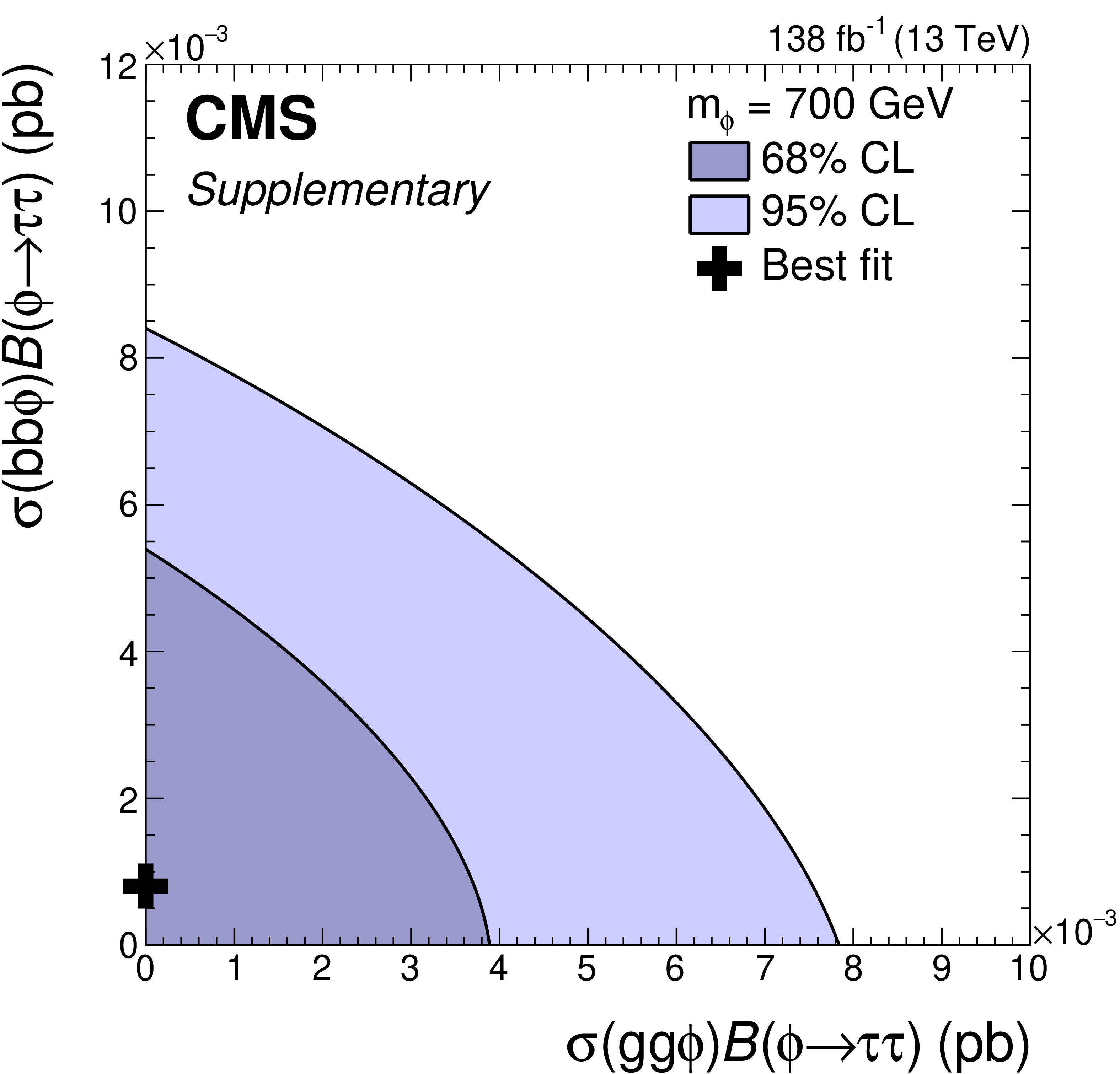
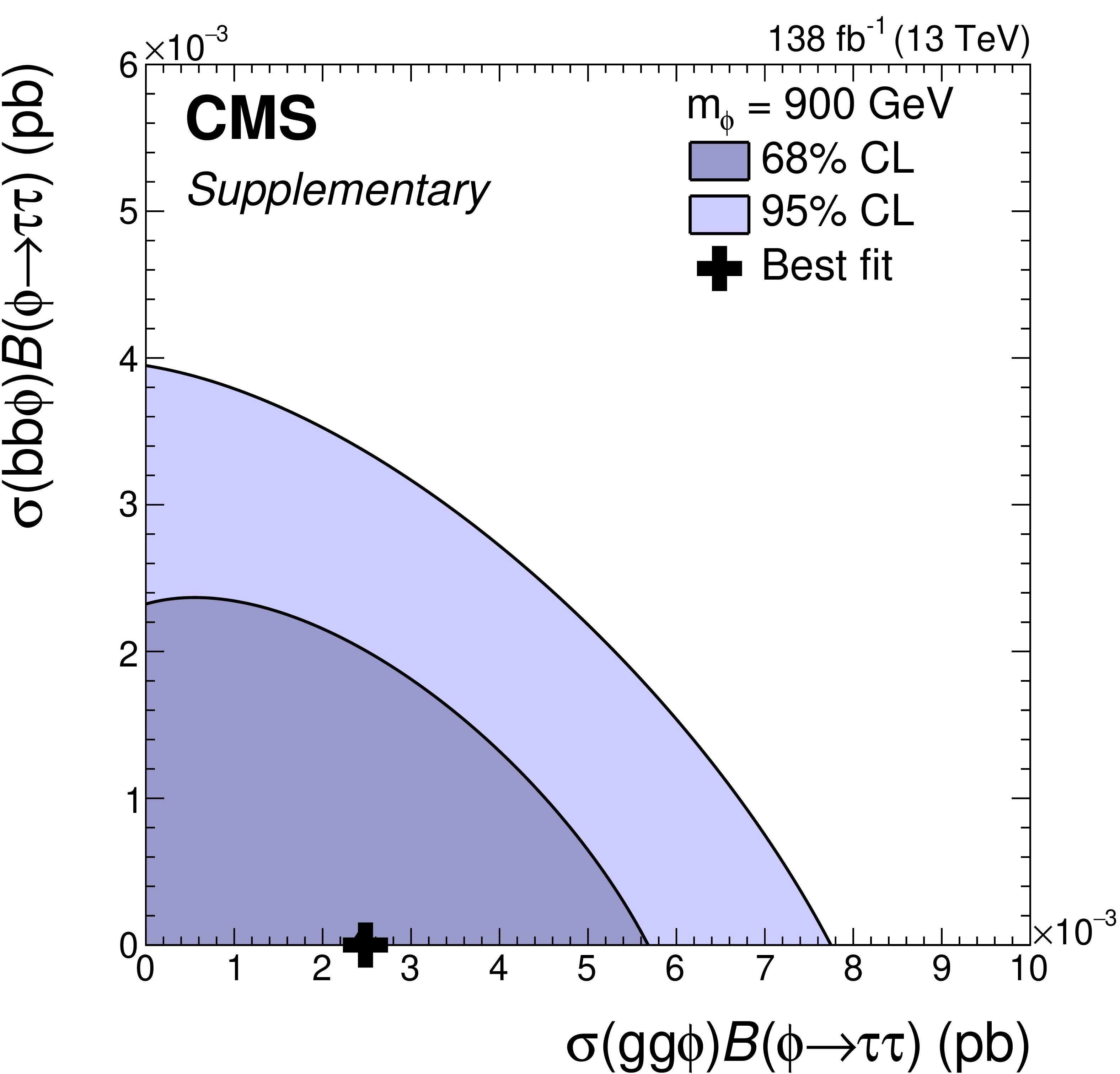
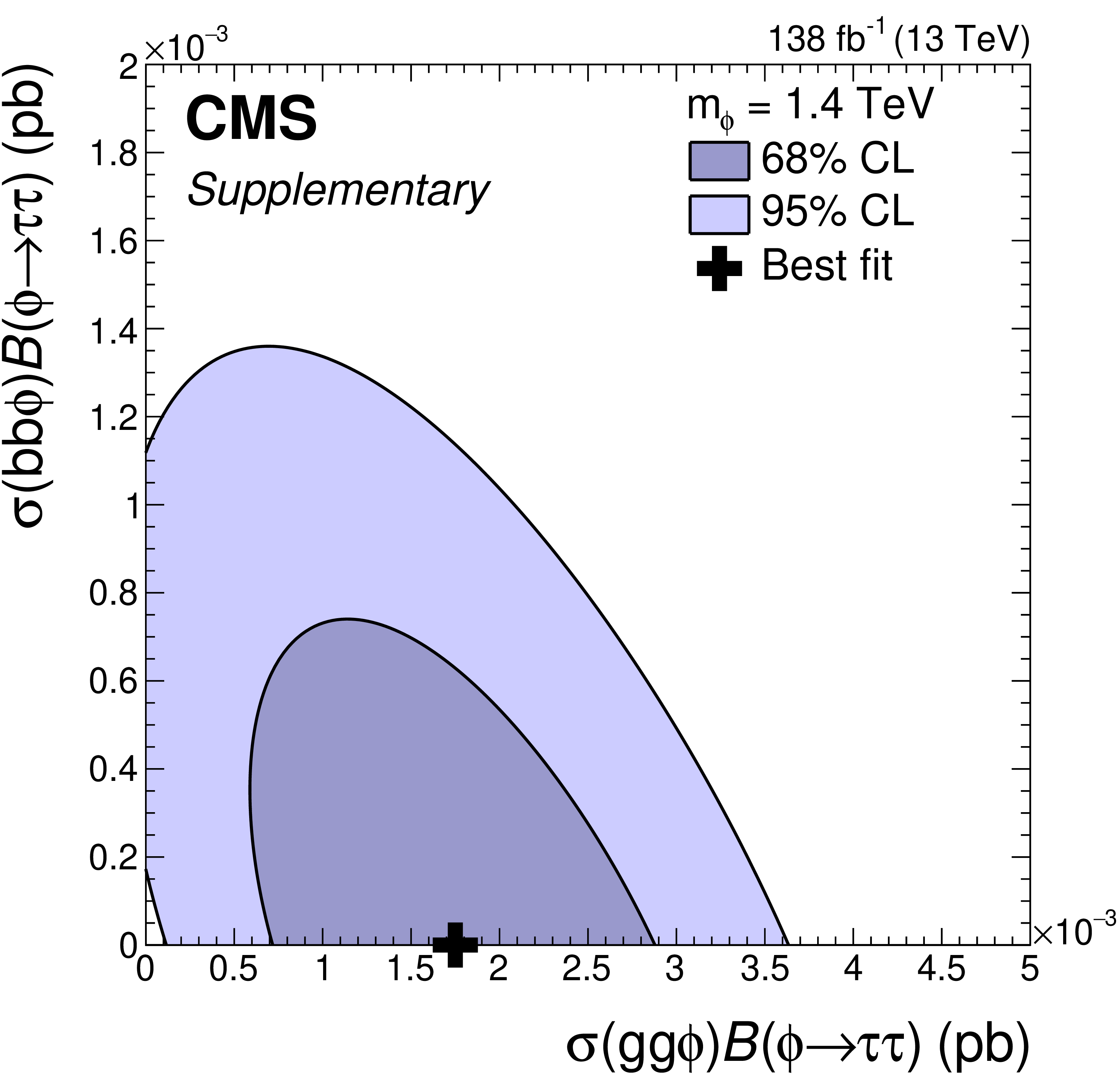
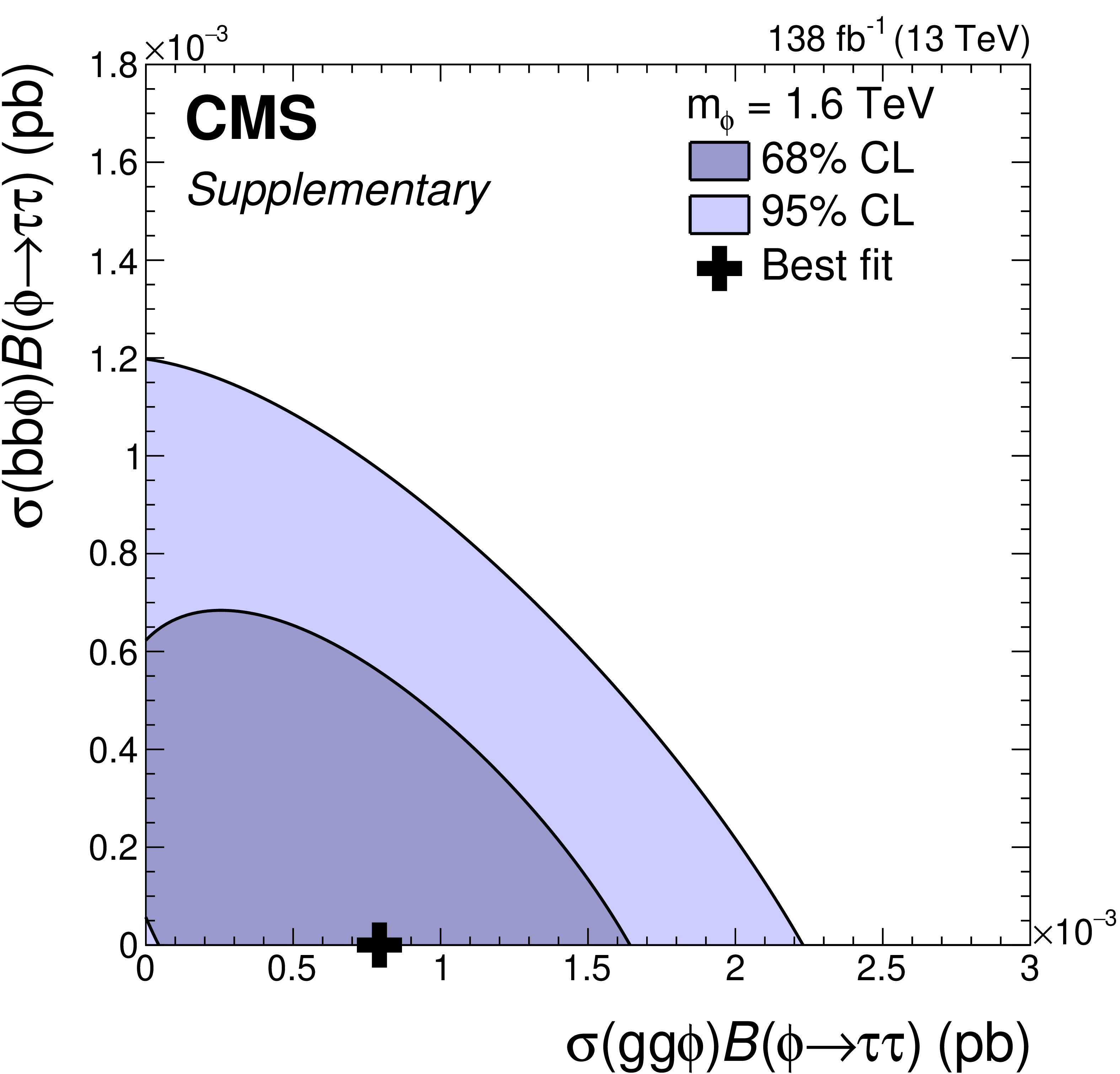
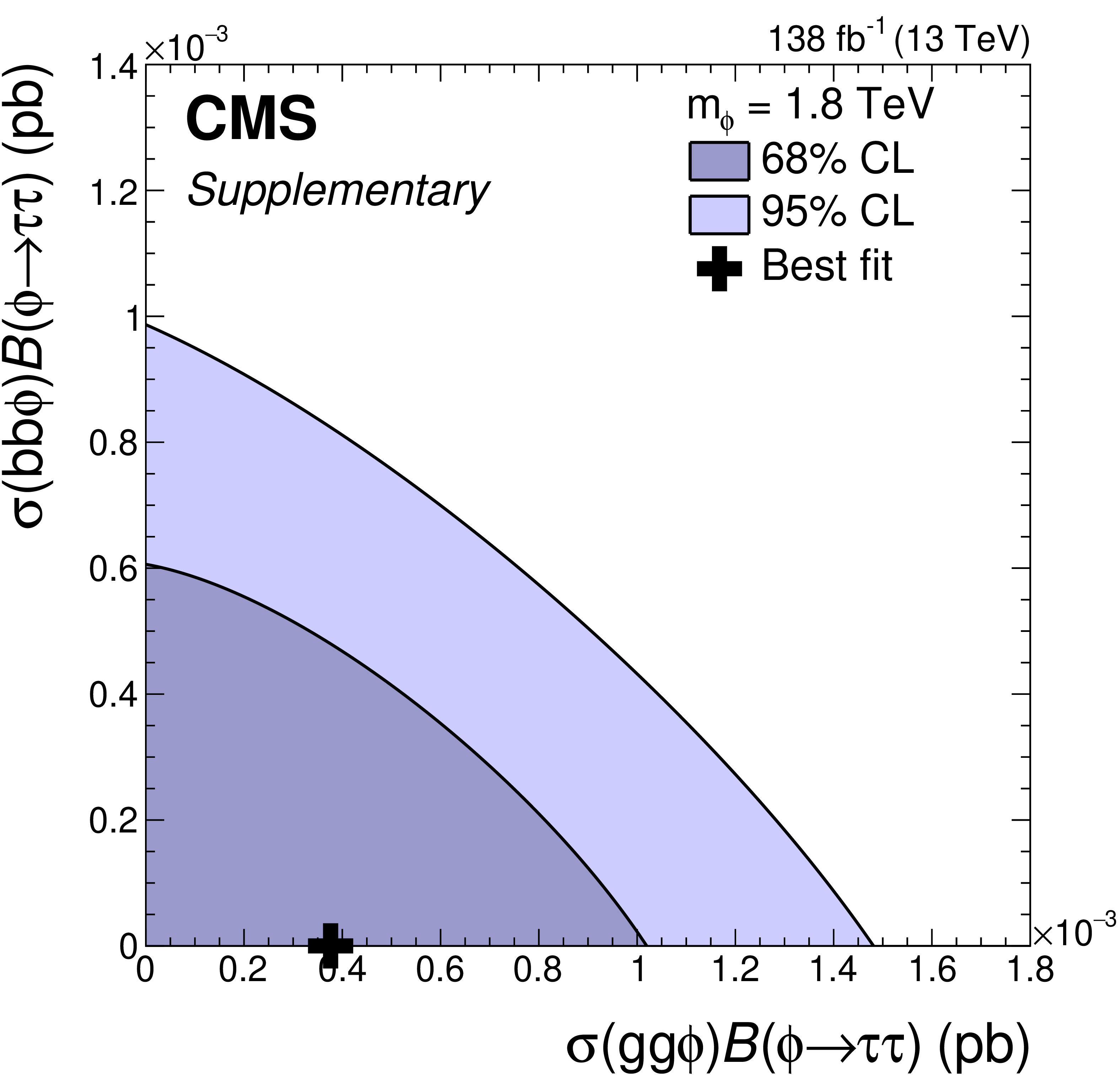
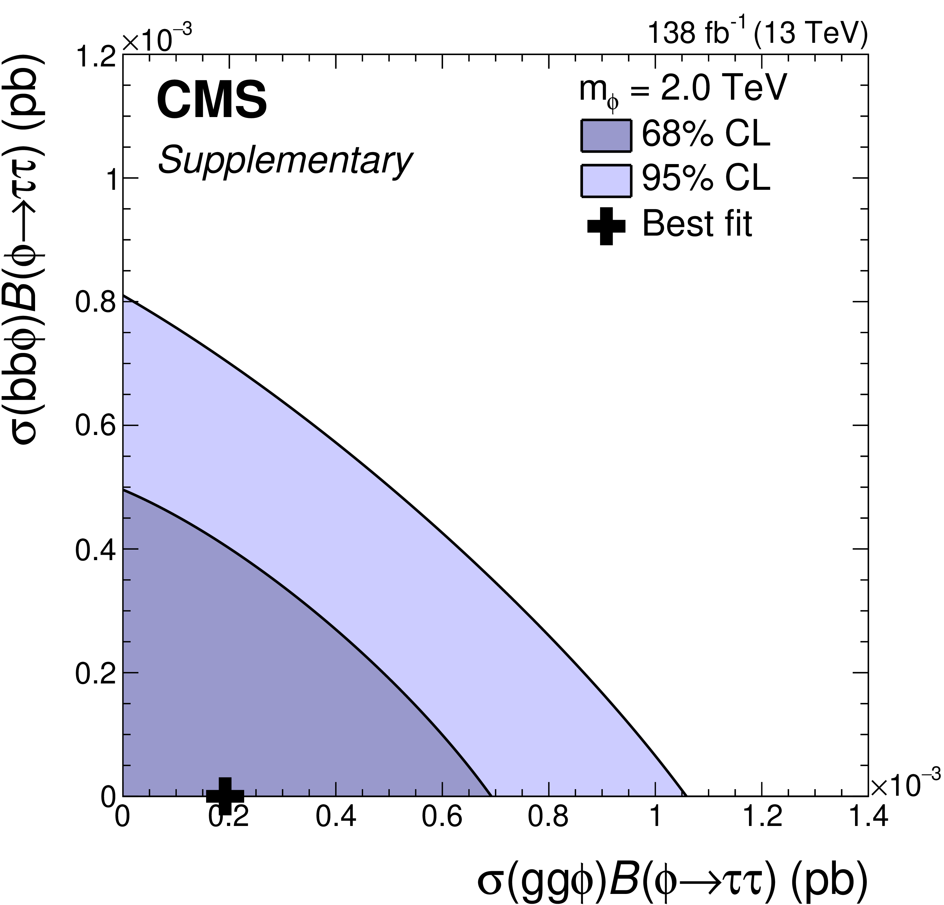
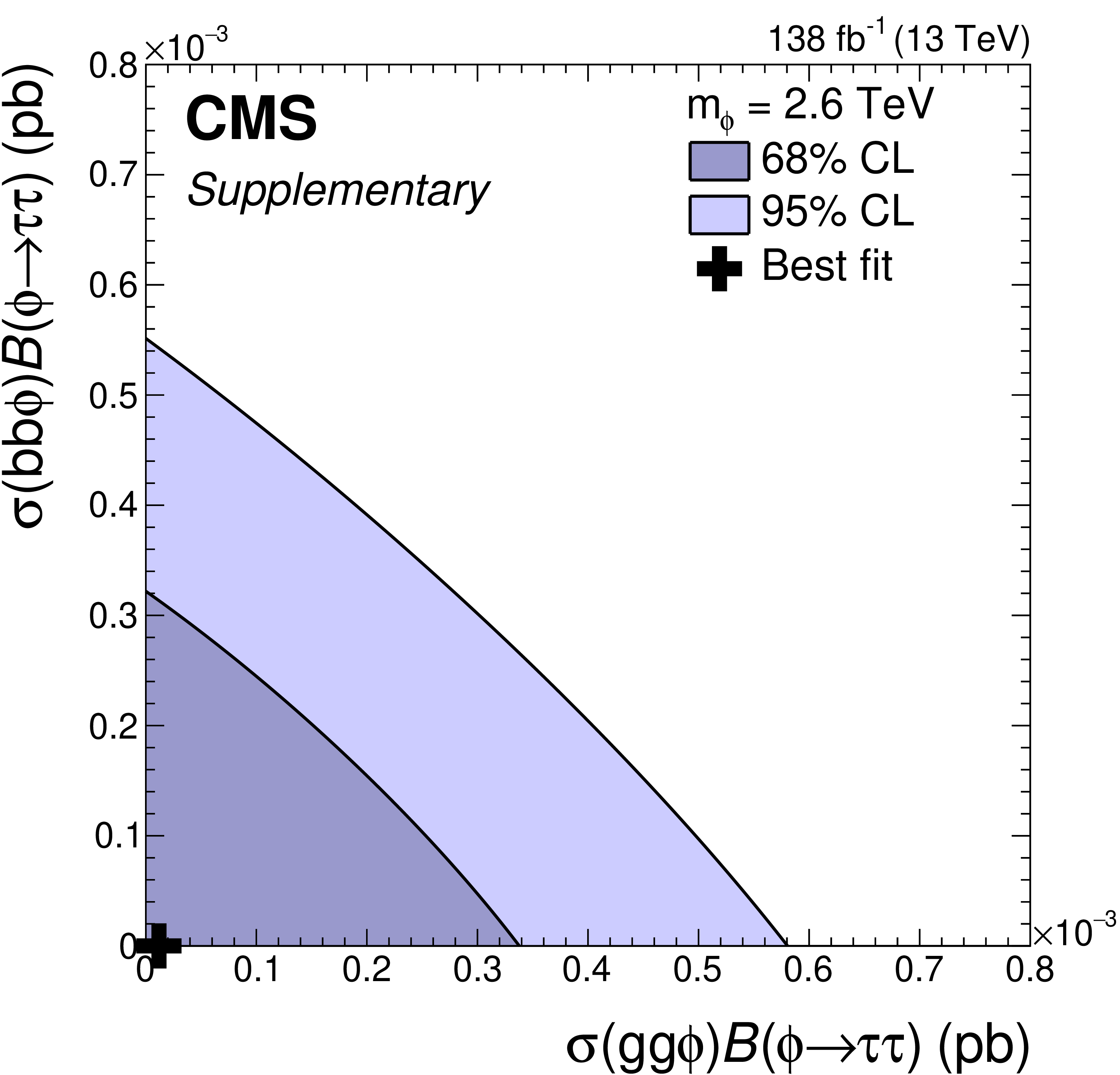
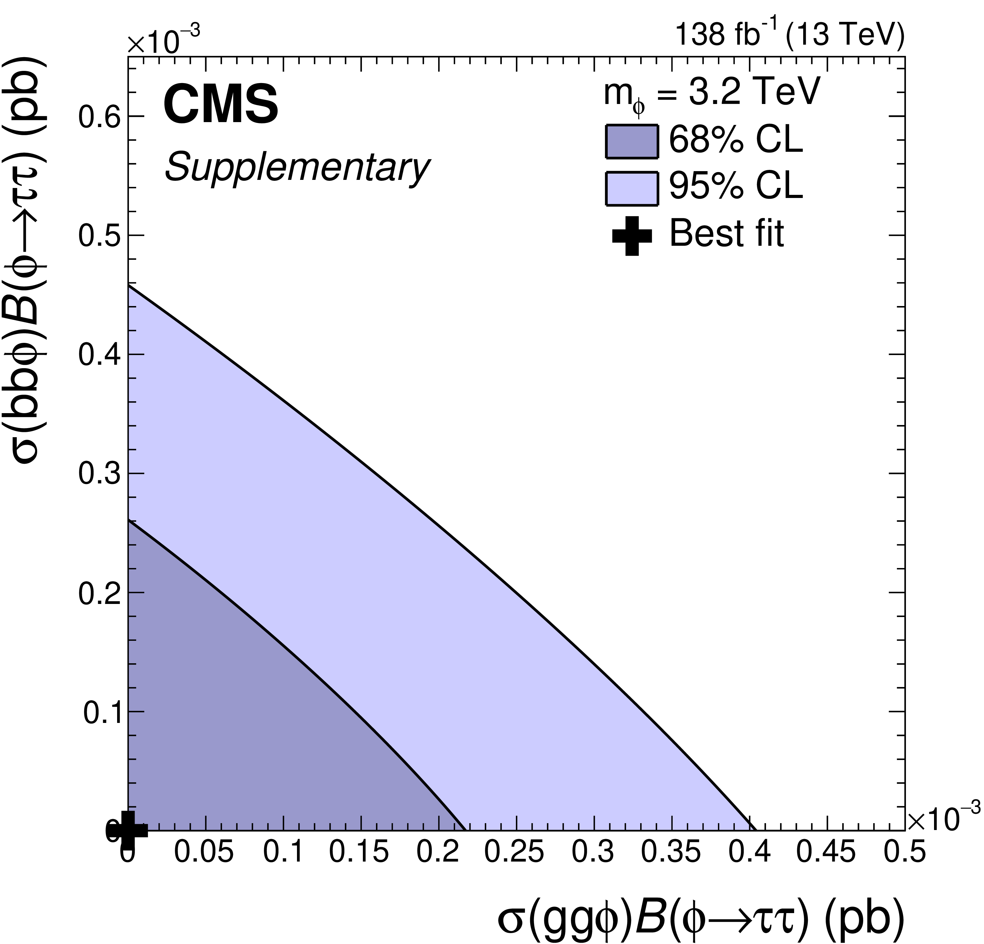
Figure 11:
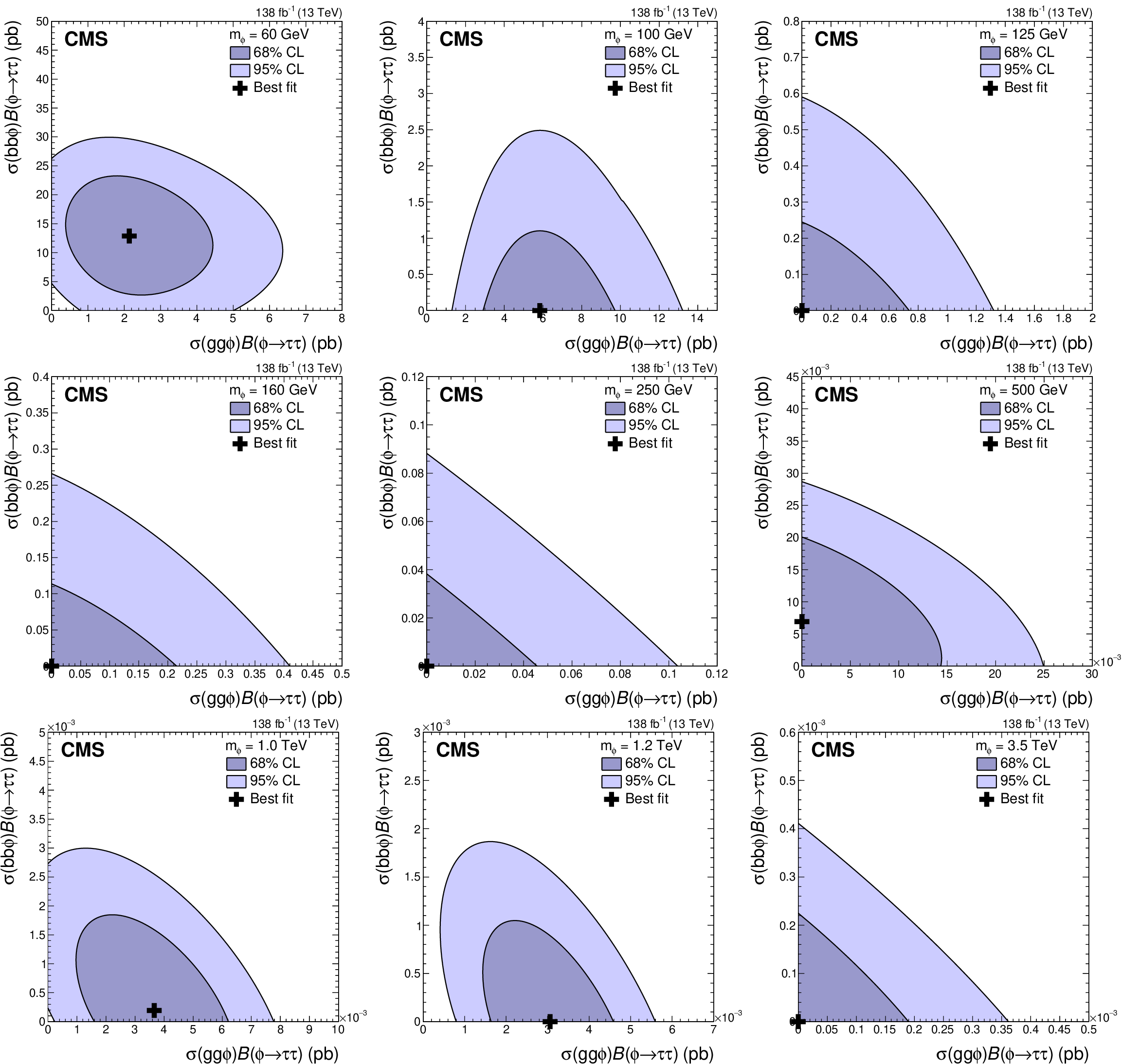
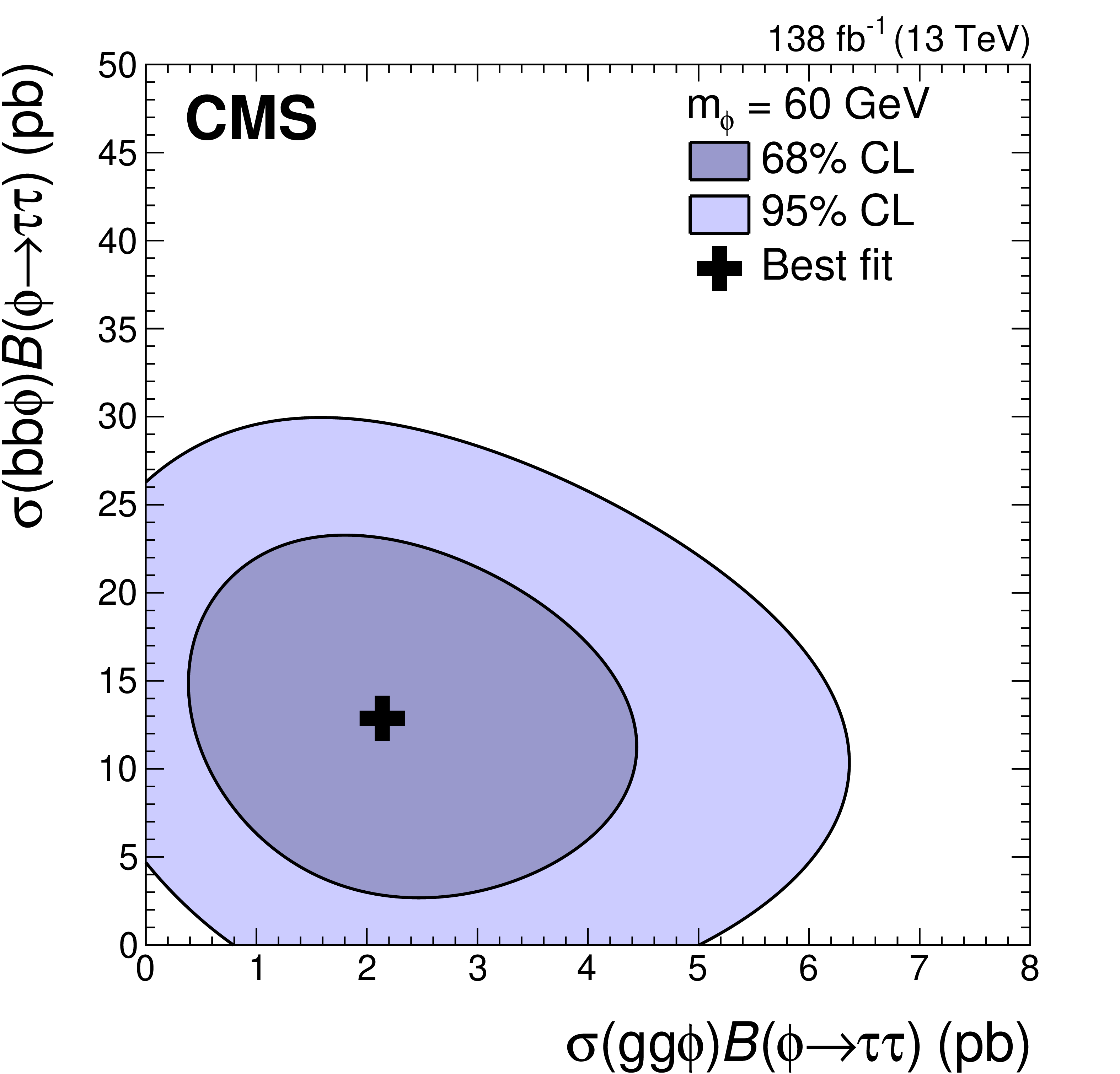
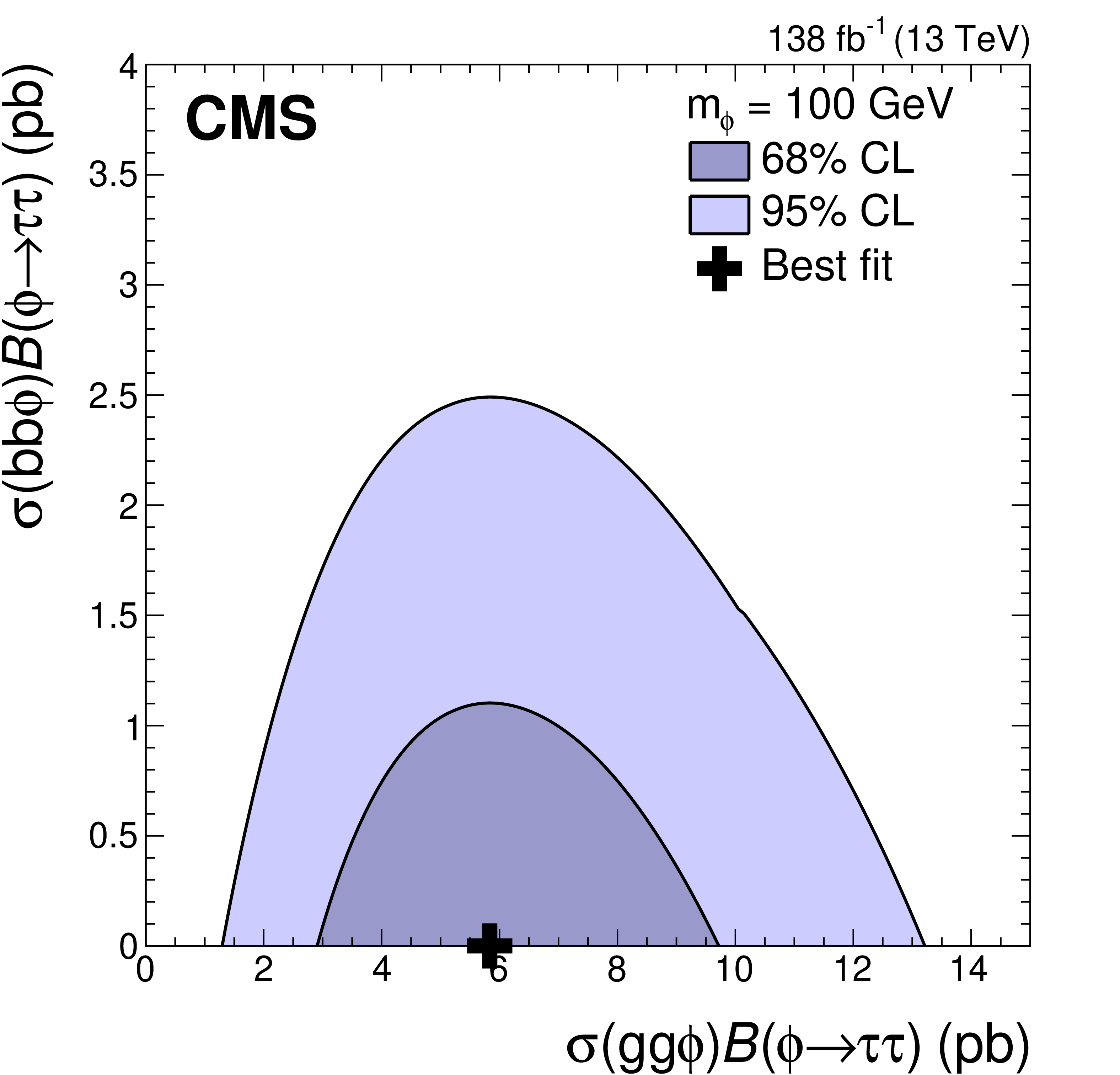
Maximum likelihood estimates, and 68% and 95% CL contours obtained from scans of the signal likelihood for the model-independent ${\phi}$ search. The scans are shown for selected values of ${m_{\phi}}$ between 60 GeV and 3.5 TeV. In each figure the SM expectation is $(0, 0)$. |
png pdf |
Figure 11-a:
Maximum likelihood estimates, and 68% and 95% CL contours obtained from scans of the signal likelihood for the model-independent ${\phi}$ search. The scans are shown for selected values of ${m_{\phi}}$ between 60 GeV and 3.5 TeV. In each figure the SM expectation is $(0, 0)$. |
png pdf |
Figure 11-b:
Maximum likelihood estimates, and 68% and 95% CL contours obtained from scans of the signal likelihood for the model-independent ${\phi}$ search. The scans are shown for selected values of ${m_{\phi}}$ between 60 GeV and 3.5 TeV. In each figure the SM expectation is $(0, 0)$. |
png pdf |
Figure 11-c:
Maximum likelihood estimates, and 68% and 95% CL contours obtained from scans of the signal likelihood for the model-independent ${\phi}$ search. The scans are shown for selected values of ${m_{\phi}}$ between 60 GeV and 3.5 TeV. In each figure the SM expectation is $(0, 0)$. |
png pdf |
Figure 11-d:
Maximum likelihood estimates, and 68% and 95% CL contours obtained from scans of the signal likelihood for the model-independent ${\phi}$ search. The scans are shown for selected values of ${m_{\phi}}$ between 60 GeV and 3.5 TeV. In each figure the SM expectation is $(0, 0)$. |

png pdf |
Figure 11-e:
Maximum likelihood estimates, and 68% and 95% CL contours obtained from scans of the signal likelihood for the model-independent ${\phi}$ search. The scans are shown for selected values of ${m_{\phi}}$ between 60 GeV and 3.5 TeV. In each figure the SM expectation is $(0, 0)$. |
png pdf |
Figure 11-f:
Maximum likelihood estimates, and 68% and 95% CL contours obtained from scans of the signal likelihood for the model-independent ${\phi}$ search. The scans are shown for selected values of ${m_{\phi}}$ between 60 GeV and 3.5 TeV. In each figure the SM expectation is $(0, 0)$. |
png pdf |
Figure 11-g:
Maximum likelihood estimates, and 68% and 95% CL contours obtained from scans of the signal likelihood for the model-independent ${\phi}$ search. The scans are shown for selected values of ${m_{\phi}}$ between 60 GeV and 3.5 TeV. In each figure the SM expectation is $(0, 0)$. |
png pdf |
Figure 11-h:
Maximum likelihood estimates, and 68% and 95% CL contours obtained from scans of the signal likelihood for the model-independent ${\phi}$ search. The scans are shown for selected values of ${m_{\phi}}$ between 60 GeV and 3.5 TeV. In each figure the SM expectation is $(0, 0)$. |
png pdf |
Figure 11-i:
Maximum likelihood estimates, and 68% and 95% CL contours obtained from scans of the signal likelihood for the model-independent ${\phi}$ search. The scans are shown for selected values of ${m_{\phi}}$ between 60 GeV and 3.5 TeV. In each figure the SM expectation is $(0, 0)$. |
png pdf |
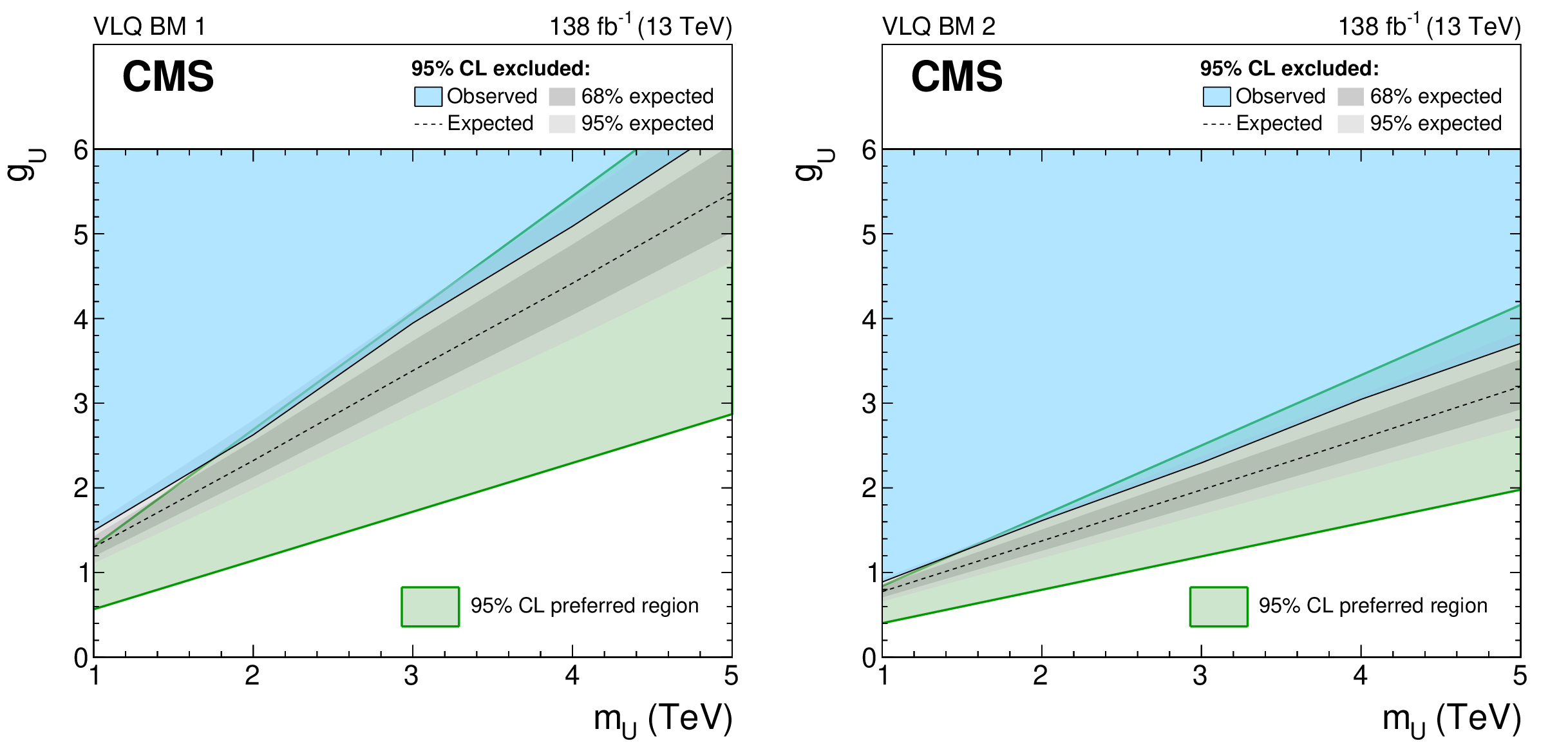
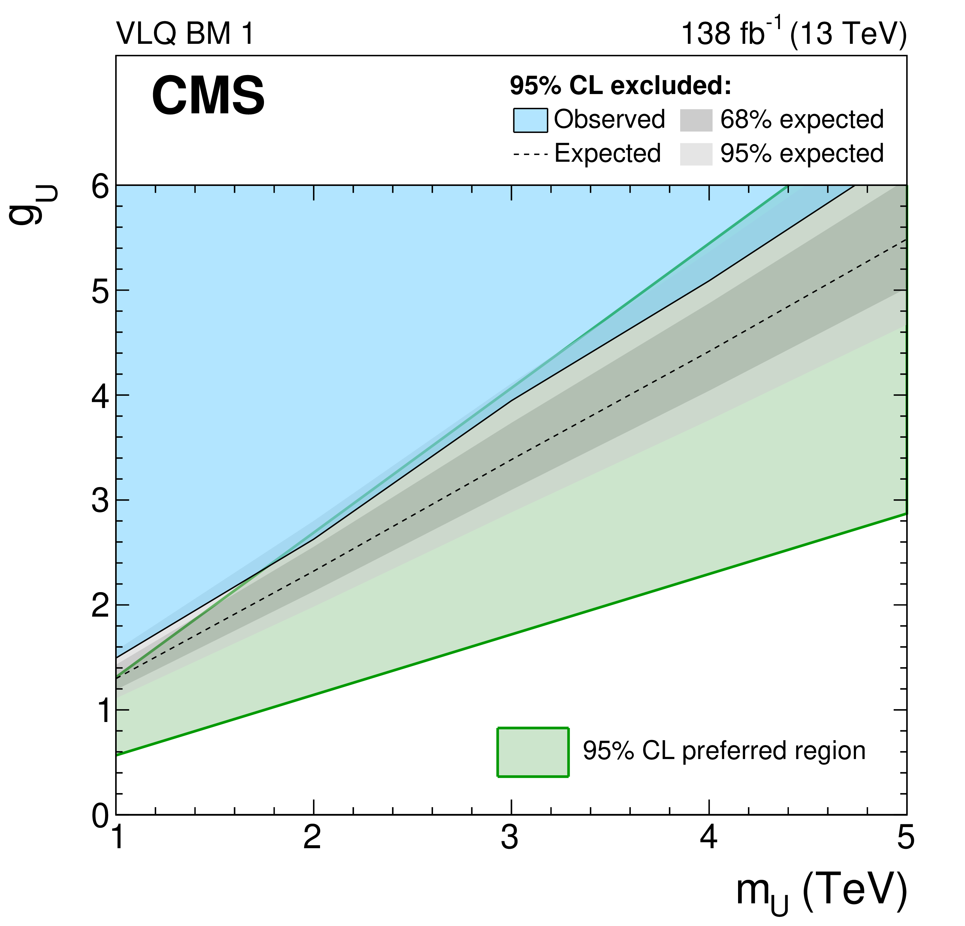
Figure 12:
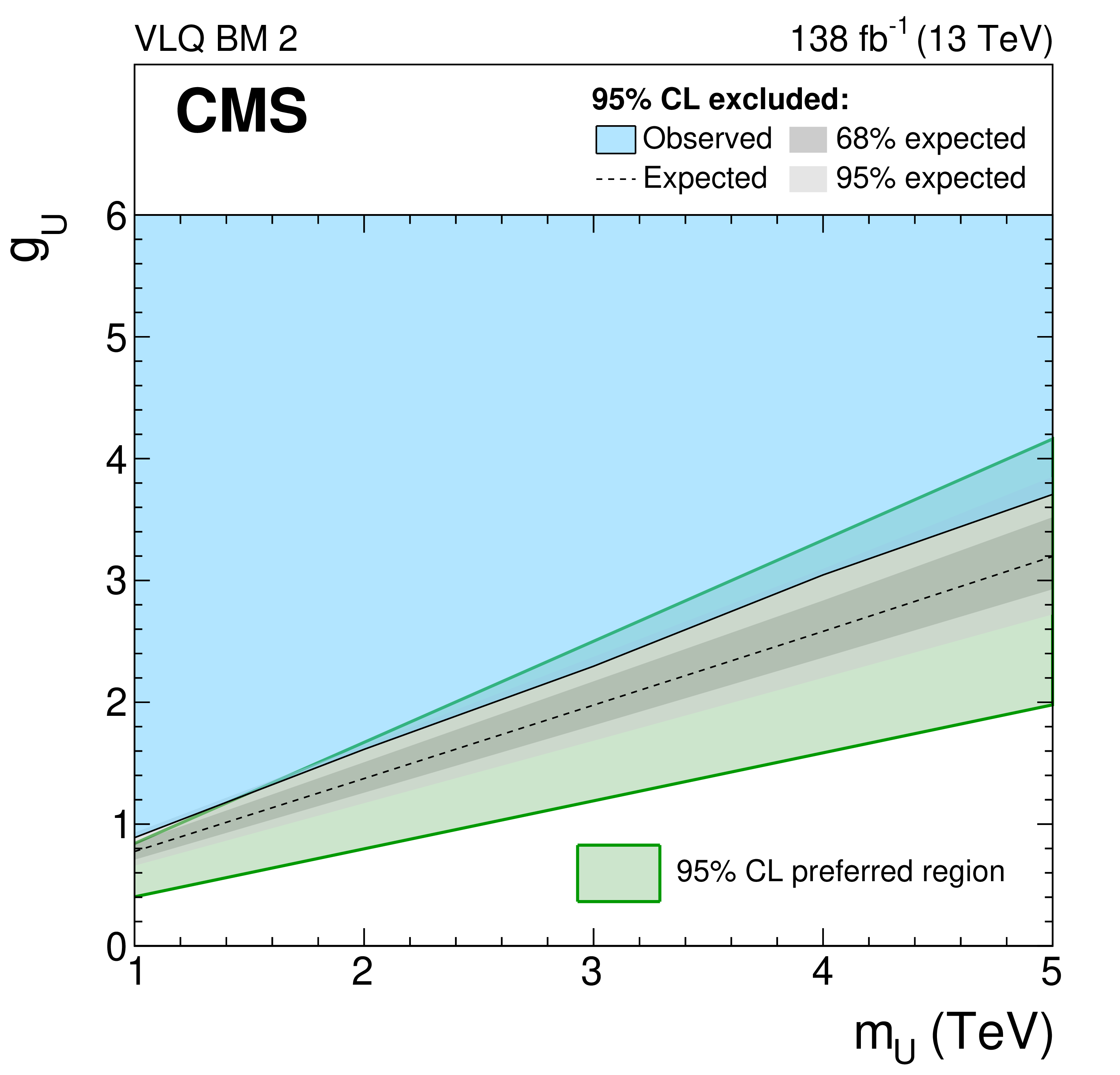
Expected and observed 95% CL upper limits on ${g_{\text {U}}}$ in the VLQ BM (left) 1 and (right) 2 scenarios, in a mass range of 1 $ < {m_{\text {U}}} < $ 5 TeV. The expected median of the exclusion limit in the absence of signal is shown by the dashed line. The dark and bright grey bands indicate the central 68% and 95% intervals of the expected exclusion limit. The observed excluded parameter space is indicated by the coloured blue area. For both scenarios, the 95% confidence interval for the preferred region from the global fit presented in Ref. [72] is also shown by the green shaded area. |
png pdf |
Figure 12-a:
Expected and observed 95% CL upper limits on ${g_{\text {U}}}$ in the VLQ BM (left) 1 and (right) 2 scenarios, in a mass range of 1 $ < {m_{\text {U}}} < $ 5 TeV. The expected median of the exclusion limit in the absence of signal is shown by the dashed line. The dark and bright grey bands indicate the central 68% and 95% intervals of the expected exclusion limit. The observed excluded parameter space is indicated by the coloured blue area. For both scenarios, the 95% confidence interval for the preferred region from the global fit presented in Ref. [72] is also shown by the green shaded area. |
png pdf |
Figure 12-b:
Expected and observed 95% CL upper limits on ${g_{\text {U}}}$ in the VLQ BM (left) 1 and (right) 2 scenarios, in a mass range of 1 $ < {m_{\text {U}}} < $ 5 TeV. The expected median of the exclusion limit in the absence of signal is shown by the dashed line. The dark and bright grey bands indicate the central 68% and 95% intervals of the expected exclusion limit. The observed excluded parameter space is indicated by the coloured blue area. For both scenarios, the 95% confidence interval for the preferred region from the global fit presented in Ref. [72] is also shown by the green shaded area. |
png pdf |
Figure 13:
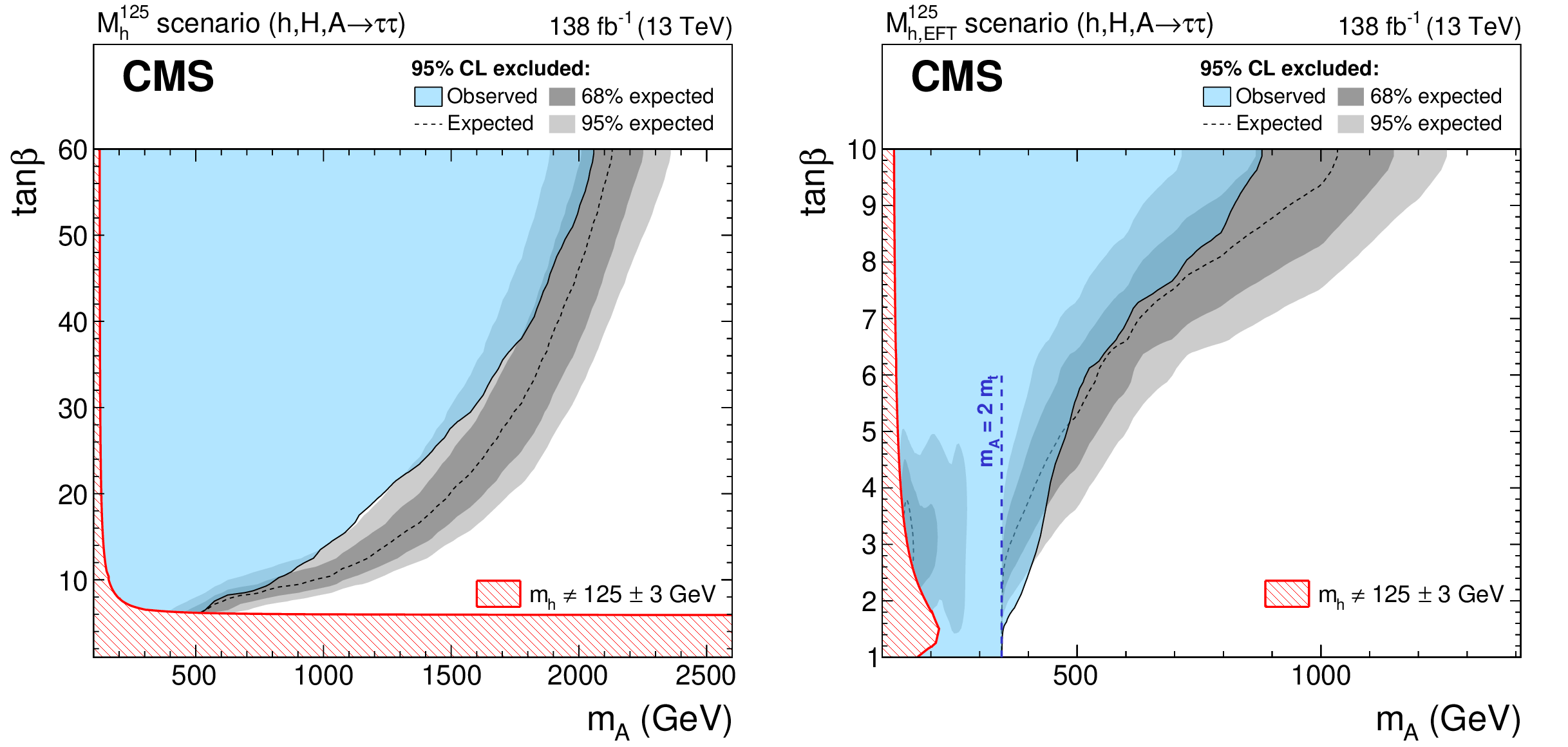
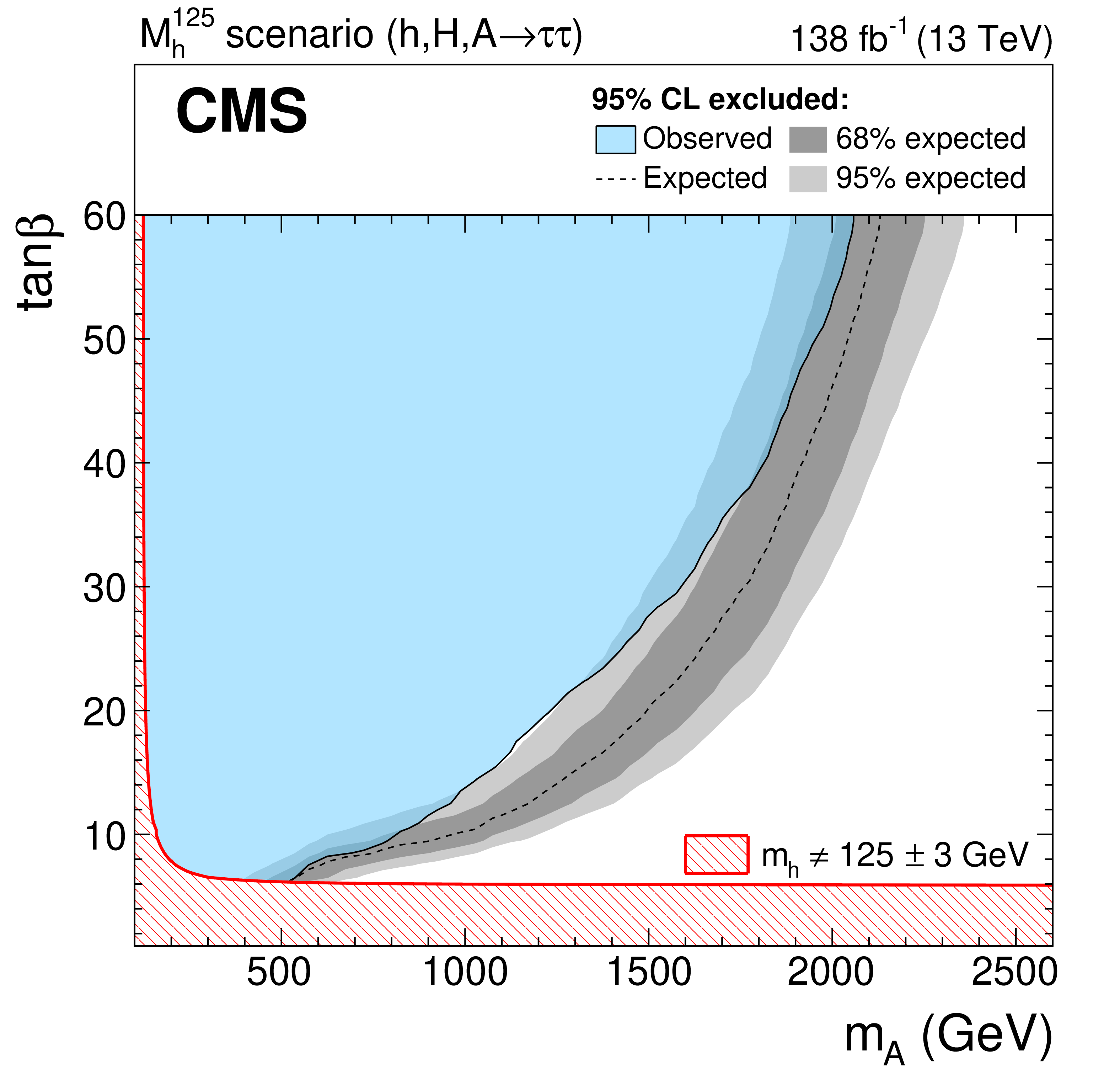
Expected and observed 95% CL exclusion contours in the MSSM (left) ${M_{\mathrm {h}}^{125}}$ and (right) ${M_{\mathrm {h},\,\text {EFT}}^{125}}$ scenarios. The expected median in the absence of a signal is shown as a dashed black line. The dark and bright grey bands indicate the central 68% and 95% intervals of the expected exclusion. The observed exclusion contour is indicated by the coloured blue area. For both scenarios, those parts of the parameter space where ${m_{\mathrm{h}}}$ deviates by more then ${\pm}$ 3 GeV from the mass of H(125) are indicated by a red hatched area. For the ${M_{\mathrm {h},\,\text {EFT}}^{125}}$ scenario, the dashed blue line indicates the threshold at $ {m_{{\mathrm {A}}}} = $ 2$ {m_{\mathrm{t}}} $ whereby the A $ \to {\mathrm{t} \mathrm{\bar{t}}} $ decay starts to influence the A $ \to \tau \tau$ branching fraction. The H $ \to \tau \tau$ branching fraction is influenced more gradually close to this threshold since A and H are not completely degenerate in mass. |
png pdf |
Figure 13-a:
Expected and observed 95% CL exclusion contours in the MSSM (left) ${M_{\mathrm {h}}^{125}}$ and (right) ${M_{\mathrm {h},\,\text {EFT}}^{125}}$ scenarios. The expected median in the absence of a signal is shown as a dashed black line. The dark and bright grey bands indicate the central 68% and 95% intervals of the expected exclusion. The observed exclusion contour is indicated by the coloured blue area. For both scenarios, those parts of the parameter space where ${m_{\mathrm{h}}}$ deviates by more then ${\pm}$ 3 GeV from the mass of H(125) are indicated by a red hatched area. For the ${M_{\mathrm {h},\,\text {EFT}}^{125}}$ scenario, the dashed blue line indicates the threshold at $ {m_{{\mathrm {A}}}} = $ 2$ {m_{\mathrm{t}}} $ whereby the A $ \to {\mathrm{t} \mathrm{\bar{t}}} $ decay starts to influence the A $ \to \tau \tau$ branching fraction. The H $ \to \tau \tau$ branching fraction is influenced more gradually close to this threshold since A and H are not completely degenerate in mass. |

png pdf |
Figure 13-b:
Expected and observed 95% CL exclusion contours in the MSSM (left) ${M_{\mathrm {h}}^{125}}$ and (right) ${M_{\mathrm {h},\,\text {EFT}}^{125}}$ scenarios. The expected median in the absence of a signal is shown as a dashed black line. The dark and bright grey bands indicate the central 68% and 95% intervals of the expected exclusion. The observed exclusion contour is indicated by the coloured blue area. For both scenarios, those parts of the parameter space where ${m_{\mathrm{h}}}$ deviates by more then ${\pm}$ 3 GeV from the mass of H(125) are indicated by a red hatched area. For the ${M_{\mathrm {h},\,\text {EFT}}^{125}}$ scenario, the dashed blue line indicates the threshold at $ {m_{{\mathrm {A}}}} = $ 2$ {m_{\mathrm{t}}} $ whereby the A $ \to {\mathrm{t} \mathrm{\bar{t}}} $ decay starts to influence the A $ \to \tau \tau$ branching fraction. The H $ \to \tau \tau$ branching fraction is influenced more gradually close to this threshold since A and H are not completely degenerate in mass. |
| Tables | |
png pdf |
Table 1:
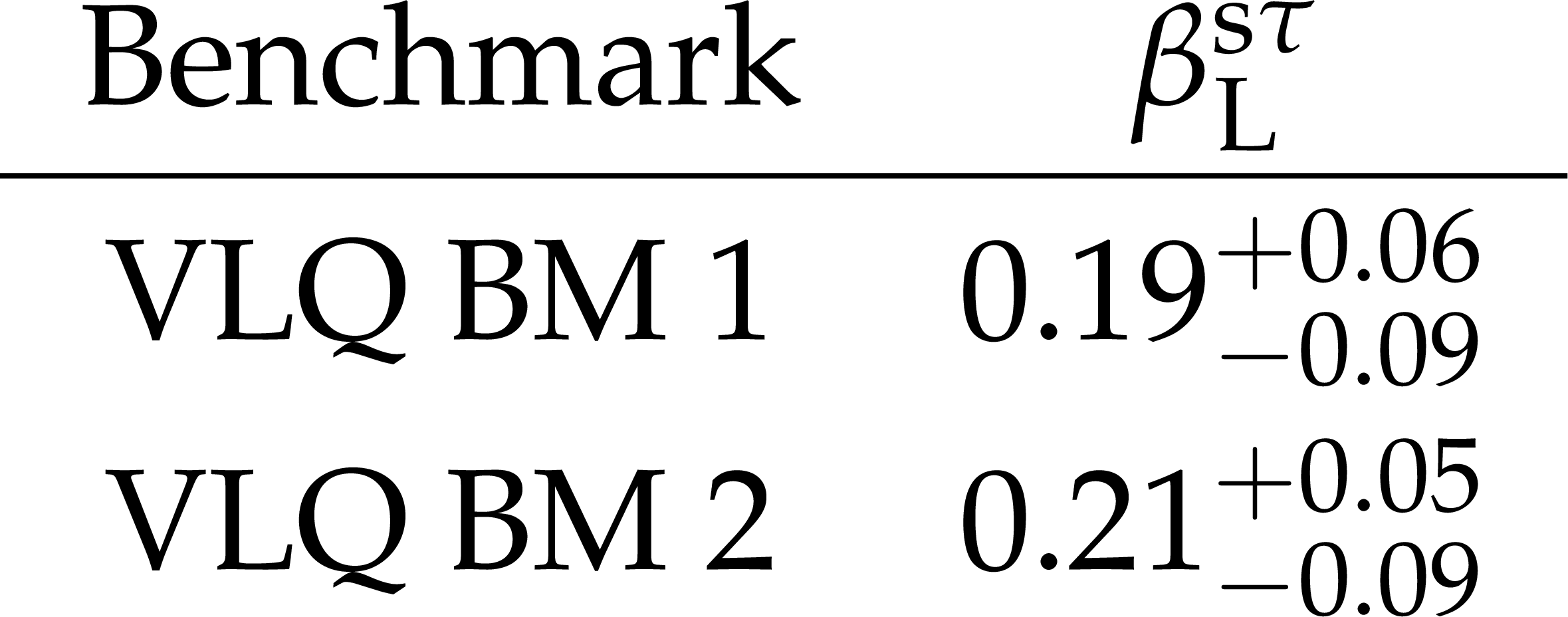
Summary of the preferred values and uncertainties of ${{\beta _{\mathrm {L}}} ^{\mathrm {s}\tau}}$ in the two considered U$_{1}$ benchmark scenarios from Ref. [72]. |
png pdf |
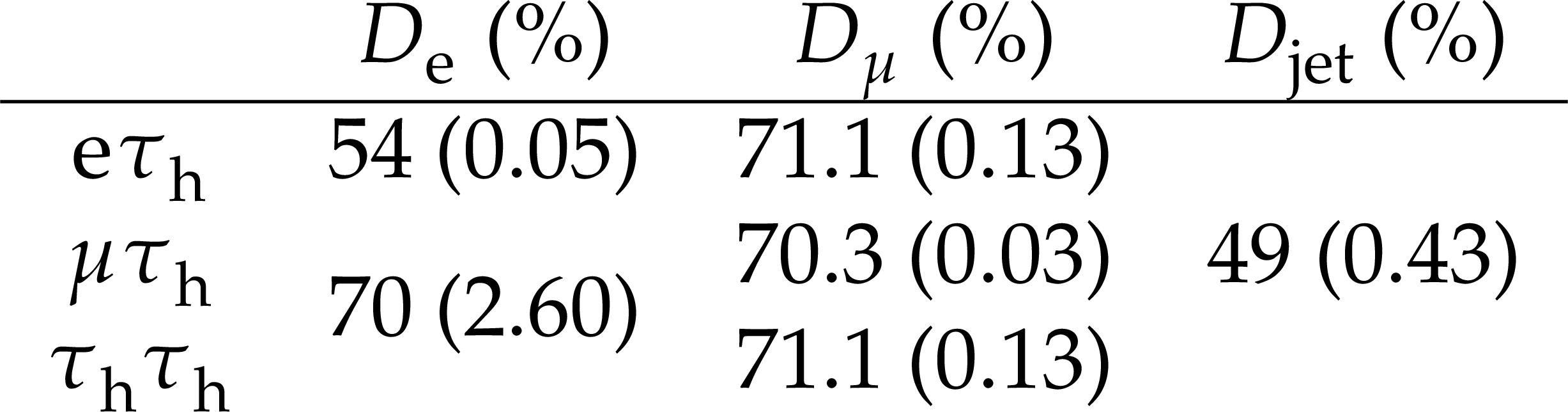
Table 2:
Efficiencies for the identification of ${\tau _\mathrm {h}}$ decays and corresponding misidentification rates (given in parentheses) for the working points of D$_{\mathrm{e}}$, D$_{\mu}$, and D$_{\text{jet}}$, chosen for the $\tau \tau$ selection, depending on the $\tau \tau$ final state. The numbers are given as a percentages. |

png pdf |
Table 3:
Offline selection requirements applied to the electron, muon, and ${\tau _\mathrm {h}}$ candidates used for the selection of the $\tau$ pair. The expressions first and second lepton refer to the label of the final state in the first column. The ${p_{\mathrm {T}}}$ requirements are given in GeV. For the e$\mu$ final state two lepton pair trigger paths, with a stronger requirement on the ${p_{\mathrm {T}}}$ of electron (muon), are used for the online selection of the event. For the e$ {\tau _\mathrm {h}}$, $\mu {\tau _\mathrm {h}}$, and ${{\tau _\mathrm {h}} {\tau _\mathrm {h}}}$ final states, the values (in parentheses) correspond to the lepton pair (single lepton) trigger paths that have been used in the online selection. A detailed discussion is given in the text. |

png pdf |
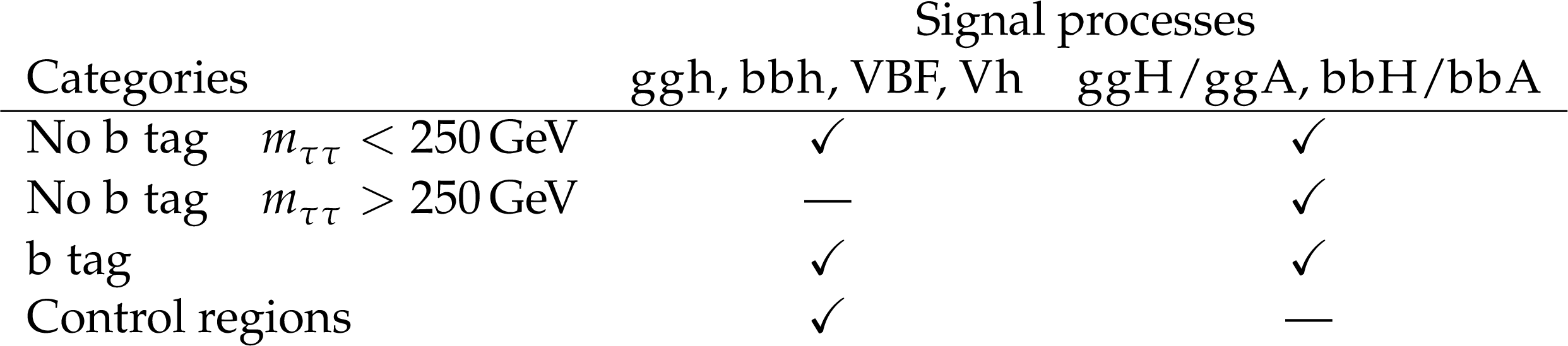
Table 4:
Event categories and discriminants used for the extraction of the signals, for the searches described in this paper. We note that ${m_{\phi}}$ refers to the hypothesized mass of the model-independent ${\phi}$ search, while ${m_{\tau \tau}}$ refers to the reconstructed mass of the $\tau \tau$ system before the decays of the $\tau$ leptons, and thus to an estimate of ${m_{\phi}}$ in data. The variable $y_{l}$ refers to the output functions of the NNs used for signal extraction in Ref. [109]. |
png pdf |
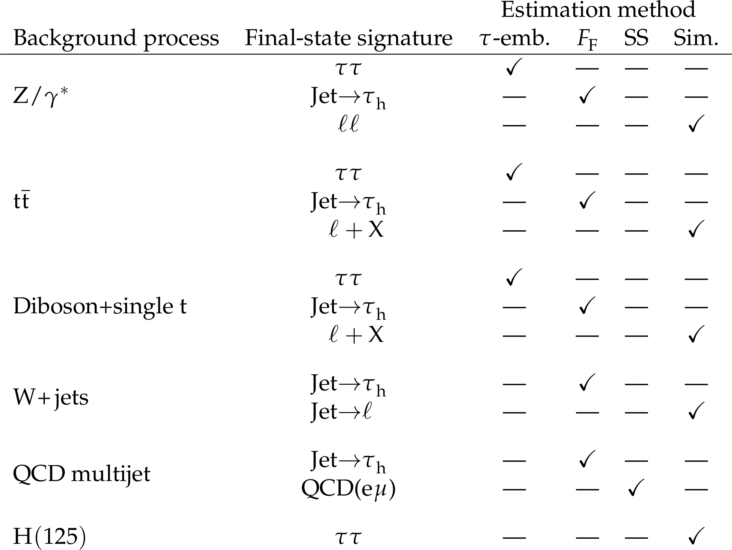
Table 5:
Background processes contributing to the event selection, as discussed in Section 5. The symbol $\ell$ corresponds to an electron or muon. The second column refers to the experimental signature in the analysis, the last four columns indicate the estimation methods used to model each corresponding signature, as described in Sections 6.1-6.4. Diboson and single t production are part of the process group iv) discussed in Section 6. QCD(e$\mu$) refers to QCD multijet production with an e$\mu$ pair in the final state. |
png pdf |
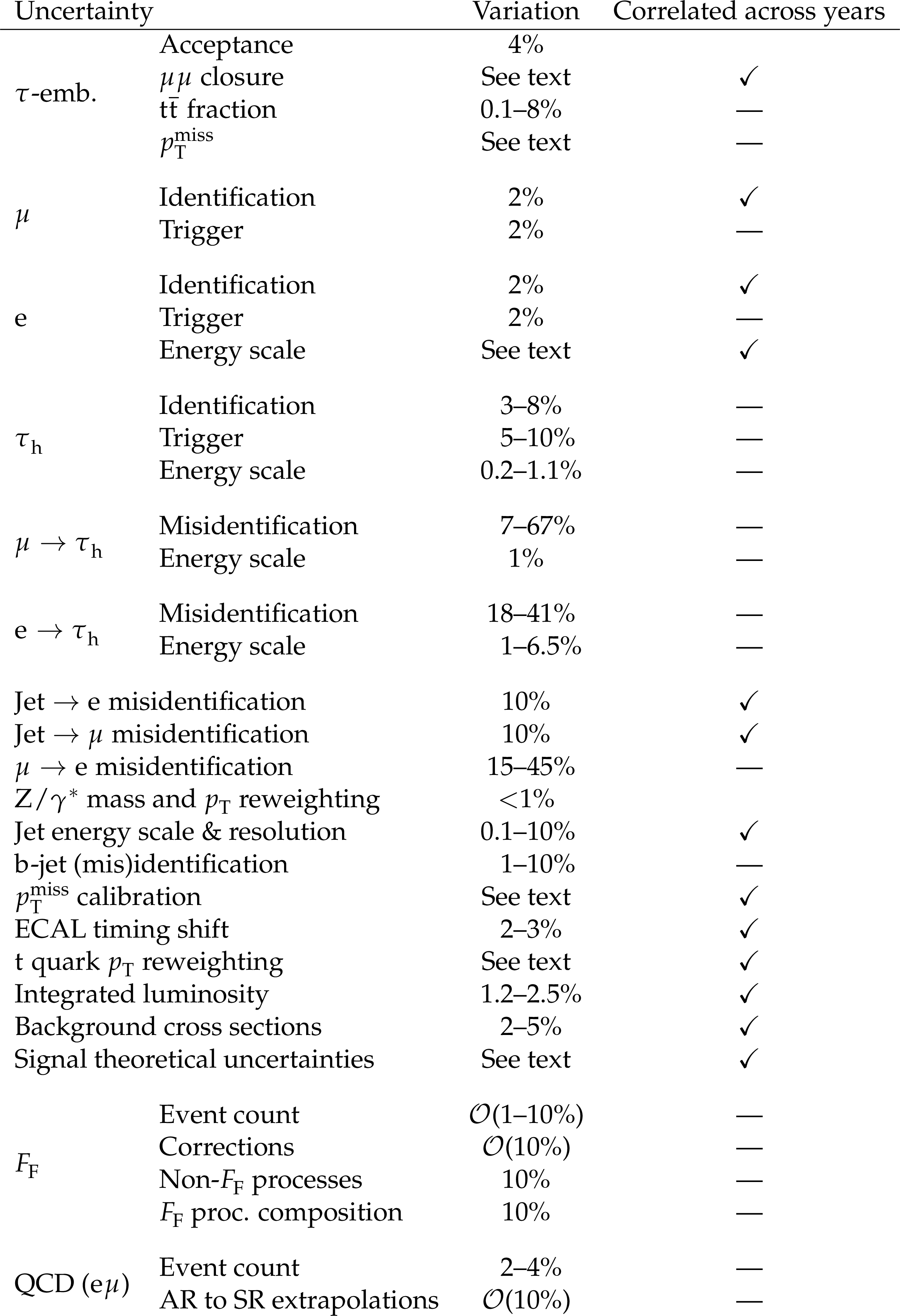
Table 6:
Summary of systematic uncertainties discussed in the text. The columns indicate the source of uncertainty, the process class that it applies to, the variation, and how it is correlated with other uncertainties. A checkmark is given also for partial correlations. More details are given in the text. |
png pdf |
Table 7:
Contribution of MSSM signals to the ${m_{\mathrm {T}}^{\text {tot}}}$ and NN output function template distributions used for signal extraction for the interpretation of the data in MSSM benchmark scenarios. |
| Summary |
| Three searches have been presented for signatures of physics beyond the standard model (SM) in $\tau\tau$ final states in proton-proton collisions at the LHC, using a data sample collected with the CMS detector at $\sqrt{s} = $ 13 TeV, corresponding to an integrated luminosity of 138 fb$^{-1}$. Upper limits at 95% confidence level (CL) have been set on the products of the branching fraction for the decay into $\tau$ leptons and the cross sections for the production of a resonance $\phi$ in addition to the observed Higgs boson via gluon fusion (gg$\phi$) or in association with b quarks, ranging from ${\mathcal{O}}$(10 pb) for a mass of 60 GeV to 0.3 fb for a mass of 3.5 TeV each. The data reveal two excesses for gg$\phi$ production with local $p$-values equivalent to about three standard deviations at ${m_{\phi}} =$ 0.1 and 1.2 TeV. Within the resolution of the reconstructed invariant mass of the $\tau\tau$ system, the excess at 100 GeV coincides with a similar excess observed in a previous search for low-mass resonances by the CMS Collaboration in the $\gamma\gamma$ final state at a mass of ${\approx}$95 GeV. In a search for $t$-channel exchange of a vector leptoquark U$_{1}$, 95% CL upper limits are set on the U$_{1}$ coupling to quarks and $\tau$ leptons ranging from 1 for a mass of 1 TeV to 6 for a mass of 5 TeV, depending on the scenario. The search is sensitive to and excludes a portion of the parameter space that can explain the b physics anomalies. In the interpretation of the ${M_{\mathrm{h}}^{125}}$ and ${M_{\mathrm{h},\,\text{EFT}}^{125}}$ minimal supersymmetric SM benchmark scenarios, additional Higgs bosons with masses below 350 GeV are excluded at 95% CL. |
| Additional Figures | |
png pdf |
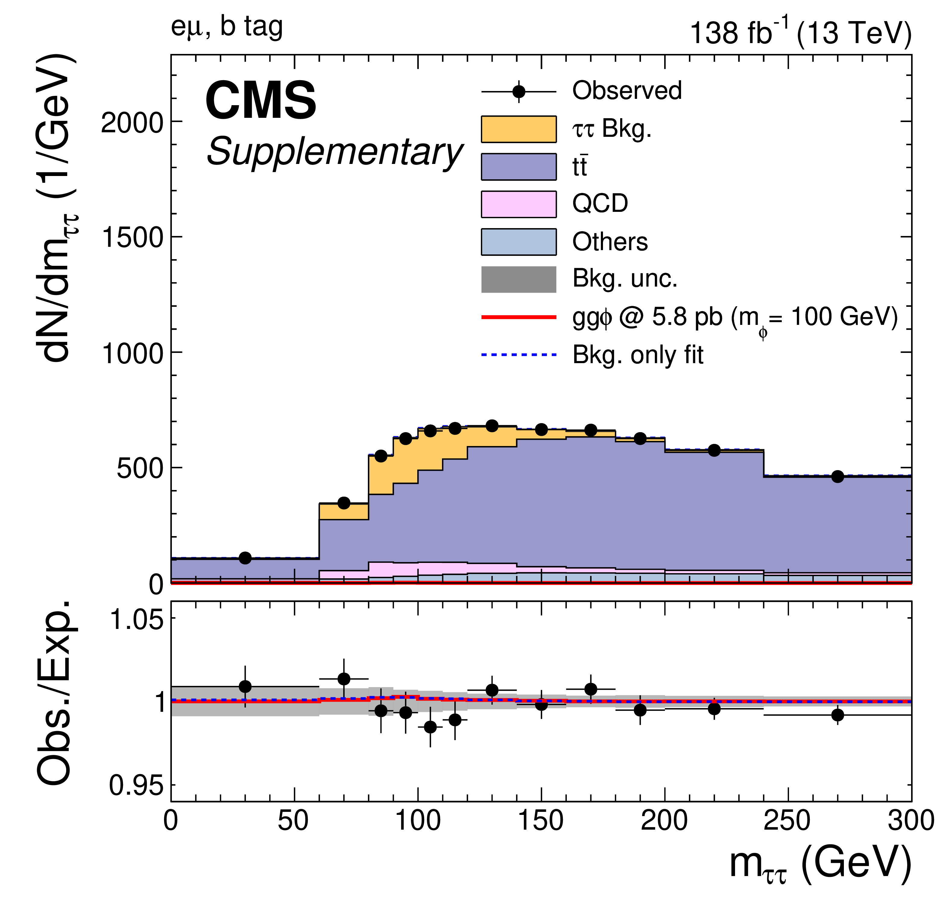
Additional Figure 1:
Distribution of $m_{ \tau \tau }$ in the ``b tag'' category used for the model-independent $\phi$ search for $m_{\phi}< $ 250 GeV, in the $ \mathrm{e} \mu $ final state. The solid histograms show the stacked background predictions after a fit of the signal-plus-background hypothesis with $m_{\phi}= $ 100 GeV to the data. The best fit $ \mathrm{g} \mathrm{g} \phi$ signal is shown by the solid red line. The total background prediction estimated from a fit of the background-only hypothesis to the data is shown by the dashed blue line for comparison. The lower panel shows the ratio of the data over the background expectation after the fit of the signal-plus-background hypothesis to the data. The full predictions of the fits of the signal-plus-background (with signal) and background-only hypotheses are also shown by the solid red and dashed blue line, respectively. |
png pdf |
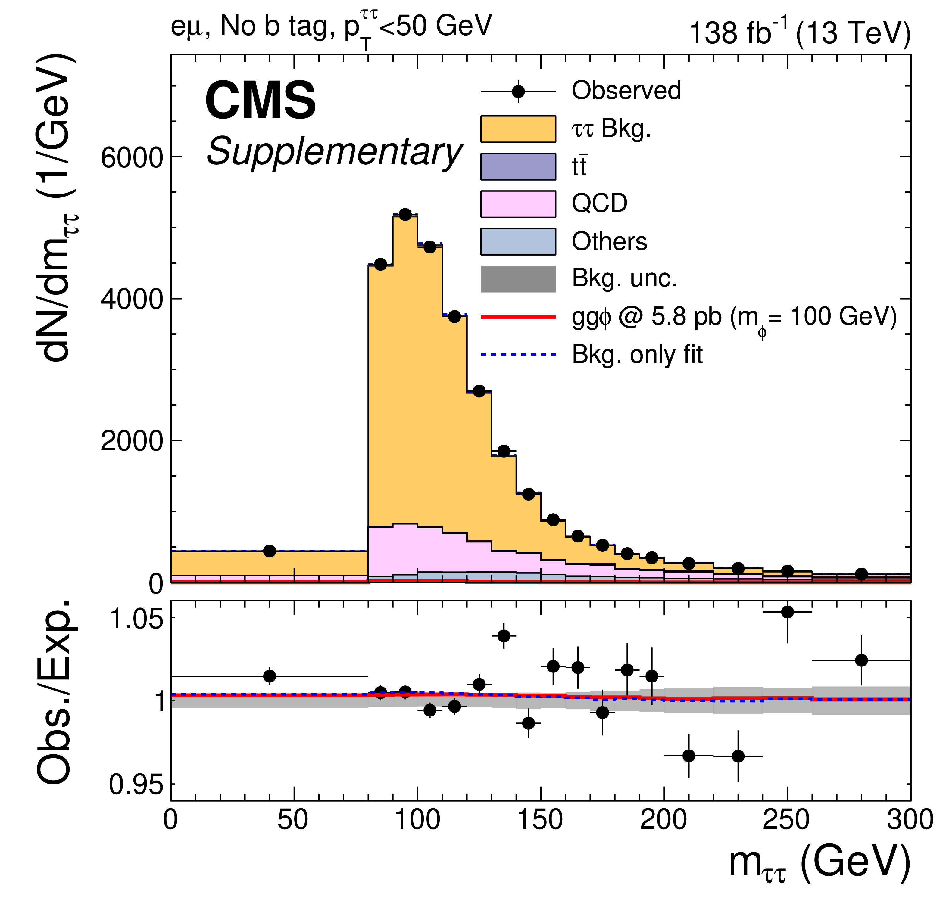
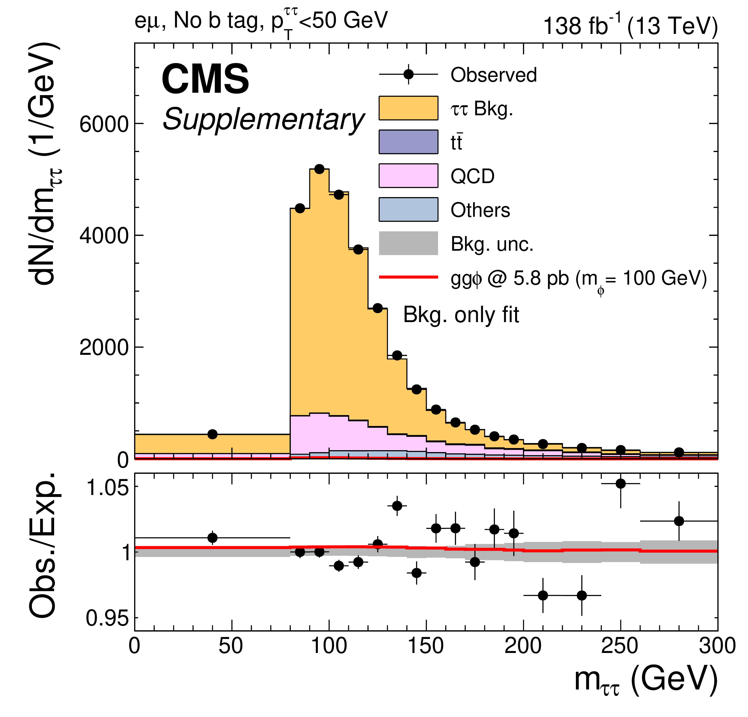
Additional Figure 2:
Distribution of $m_{ \tau \tau }$ in the ``No b tag, $ p_{\mathrm{T}} ^{ \tau \tau }< $ 50 GeV'' category used for the model-independent $\phi$ search for $m_{\phi}< $ 250 GeV, in the $ \mathrm{e} \mu $ final state. The solid histograms show the stacked background predictions after a fit of the signal-plus-background hypothesis with $m_{\phi}= $ 100 GeV to the data. The best fit $ \mathrm{g} \mathrm{g} \phi$ signal is shown by the solid red line. The total background prediction estimated from a fit of the background-only hypothesis to the data is shown by the dashed blue line for comparison. The lower panel shows the ratio of the data over the background expectation after the fit of the signal-plus-background hypothesis to the data. The full predictions of the fits of the signal-plus-background (with signal) and background-only hypotheses are also shown by the solid red and dashed blue line, respectively. |
png pdf |
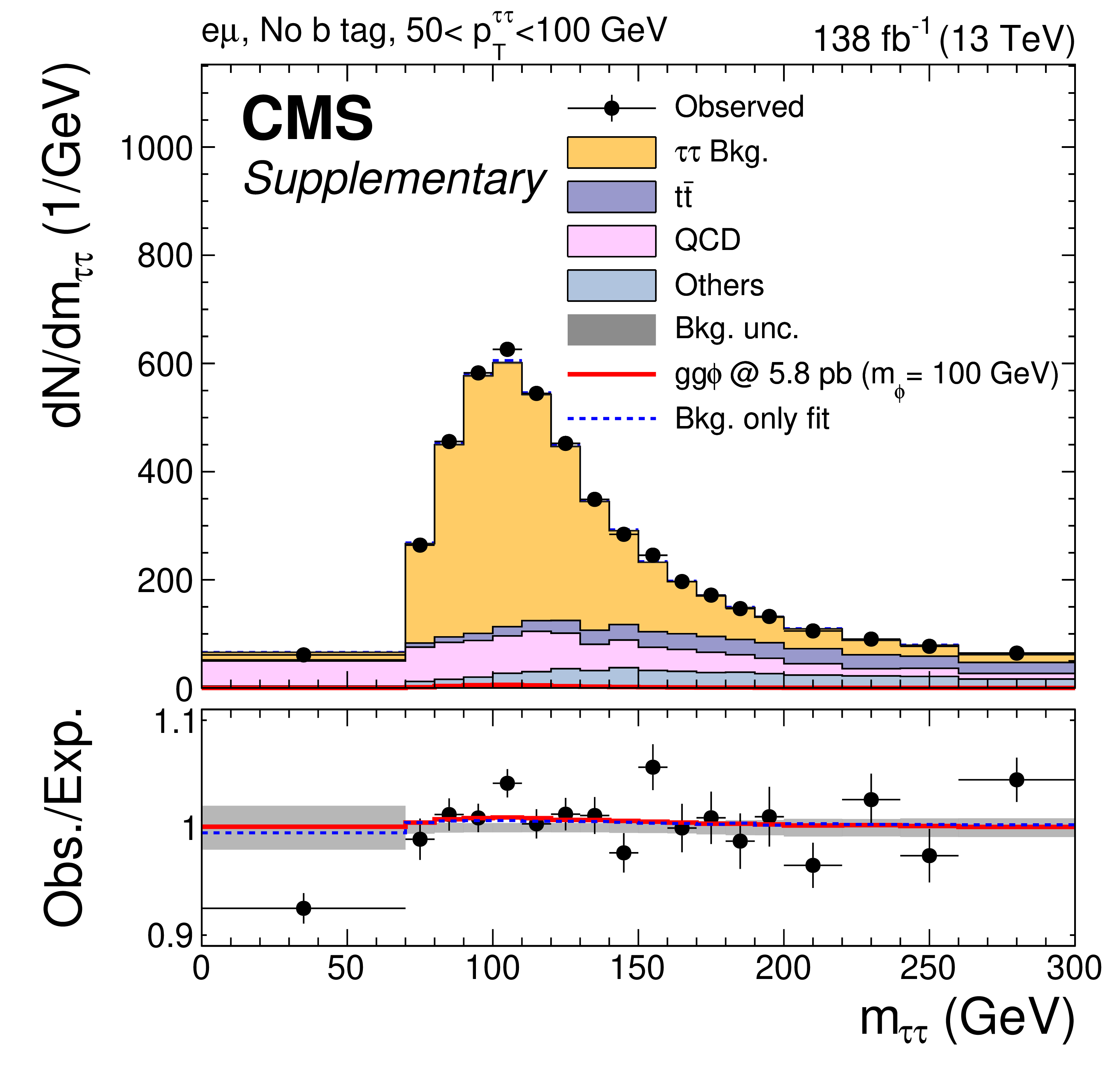
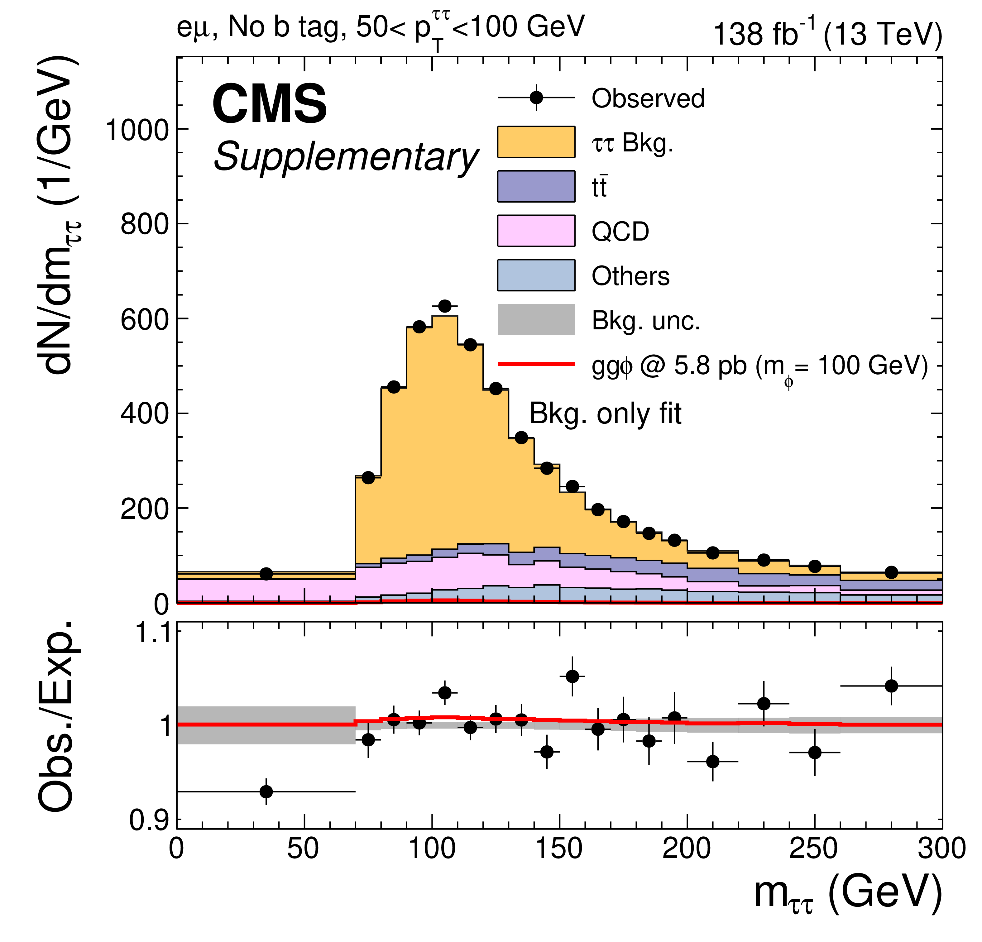
Additional Figure 3:
Distribution of $m_{ \tau \tau }$ in the ``No b tag, 50 $ < p_{\mathrm{T}} ^{ \tau \tau }< $ 100 GeV'' category used for the model-independent $\phi$ search for $m_{\phi}< $ 250 GeV, in the $ \mathrm{e} \mu $ final state. The solid histograms show the stacked background predictions after a fit of the signal-plus-background hypothesis with $m_{\phi}= $ 100 GeV to the data. The best fit $ \mathrm{g} \mathrm{g} \phi$ signal is shown by the solid red line. The total background prediction estimated from a fit of the background-only hypothesis to the data is shown by the dashed blue line for comparison. The lower panel shows the ratio of the data over the background expectation after the fit of the signal-plus-background hypothesis to the data. The full predictions of the fits of the signal-plus-background (with signal) and background-only hypotheses are also shown by the solid red and dashed blue line, respectively. |

png pdf |
Additional Figure 4:
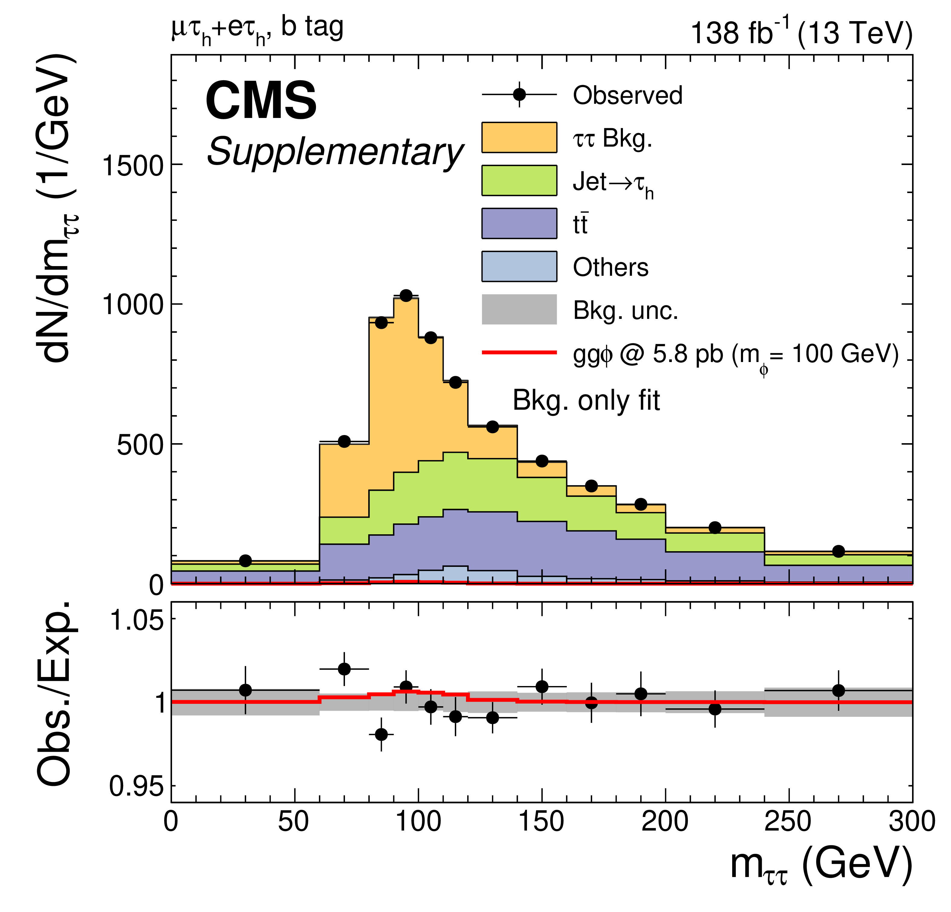
Distribution of $m_{ \tau \tau }$ in the ``b tag'' category used for the model-independent $\phi$ search for $m_{\phi}< $ 250 GeV, in the $ \mathrm{e} \tau _{\mathrm{h}}$ and $ \mu \tau _{\mathrm{h}}$ final states combined. The solid histograms show the stacked background predictions after a fit of the signal-plus-background hypothesis with $m_{\phi}= $ 100 GeV to the data. The best fit $ \mathrm{g} \mathrm{g} \phi$ signal is shown by the solid red line. The total background prediction estimated from a fit of the background-only hypothesis to the data is shown by the dashed blue line for comparison. The lower panel shows the ratio of the data over the background expectation after the fit of the signal-plus-background hypothesis to the data. The full predictions of the fits of the signal-plus-background (with signal) and background-only hypotheses are also shown by the solid red and dashed blue line, respectively. |

png pdf |
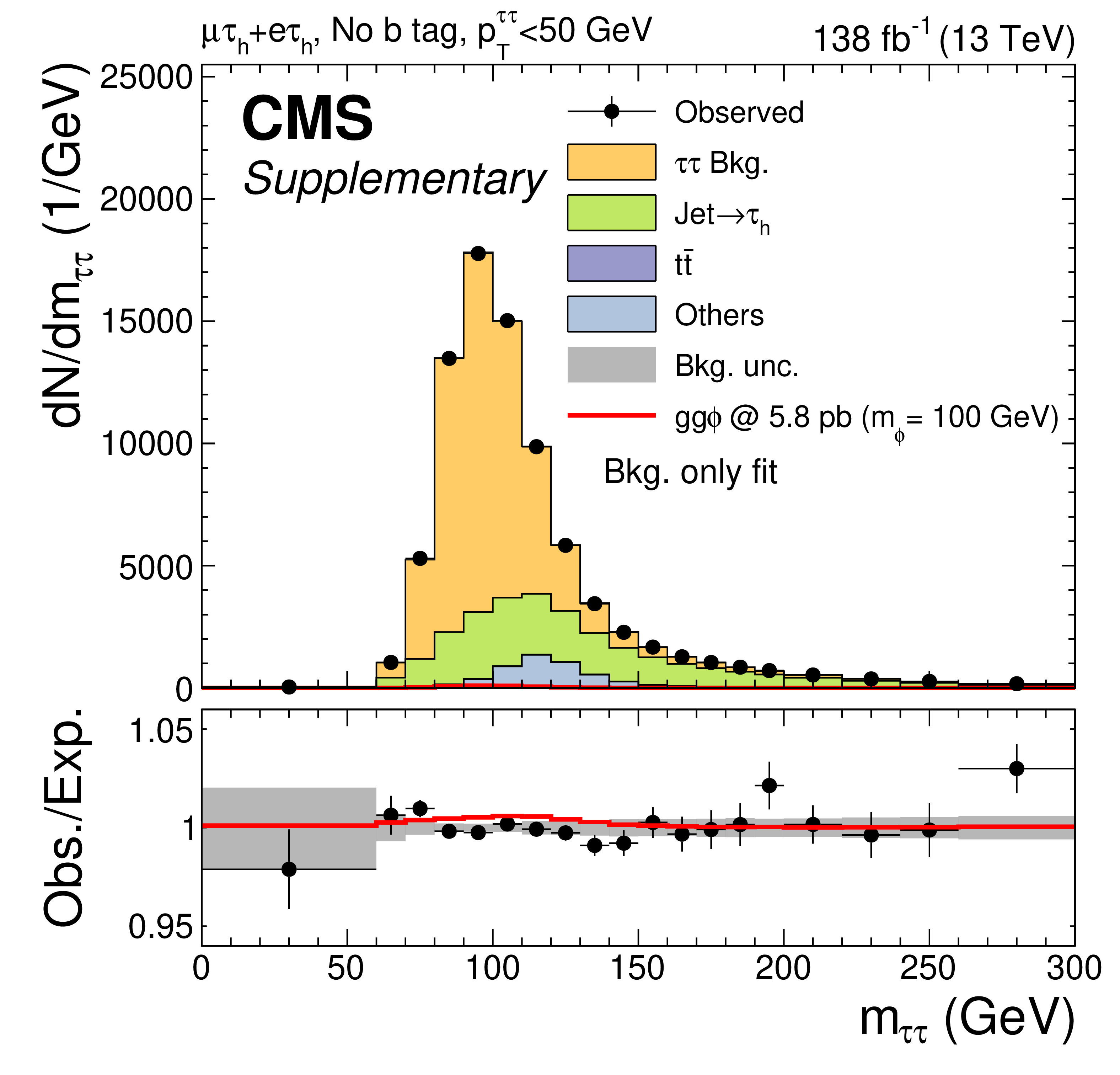
Additional Figure 5:
Distribution of $m_{ \tau \tau }$ in the ``No b tag, $ p_{\mathrm{T}} ^{ \tau \tau }< $ 50 GeV'' category used for the model-independent $\phi$ search for $m_{\phi}< $ 250 GeV, in the $ \mathrm{e} \tau _{\mathrm{h}}$ and $ \mu \tau _{\mathrm{h}}$ final states combined. The solid histograms show the stacked background predictions after a fit of the signal-plus-background hypothesis with $m_{\phi}= $ 100 GeV to the data. The best fit $ \mathrm{g} \mathrm{g} \phi$ signal is shown by the solid red line. The total background prediction estimated from a fit of the background-only hypothesis to the data is shown by the dashed blue line for comparison. The lower panel shows the ratio of the data over the background expectation after the fit of the signal-plus-background hypothesis to the data. The full predictions of the fits of the signal-plus-background (with signal) and background-only hypotheses are also shown by the solid red and dashed blue line, respectively. |
png pdf |
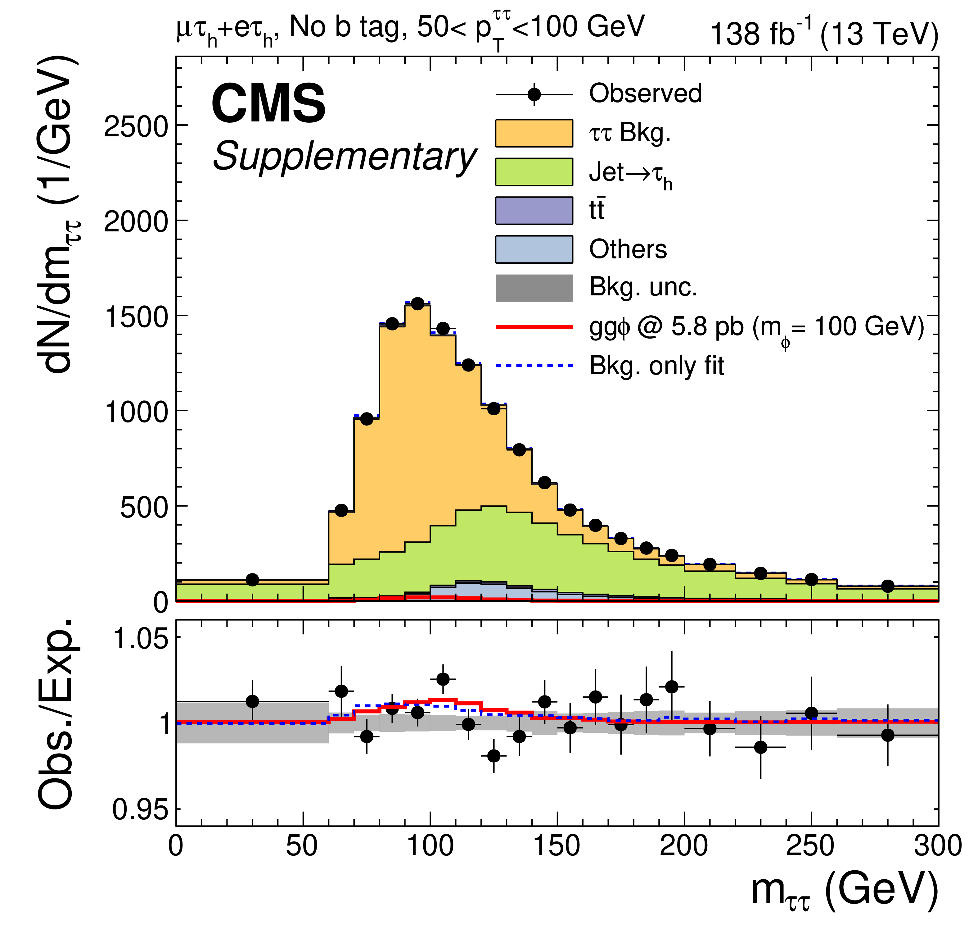
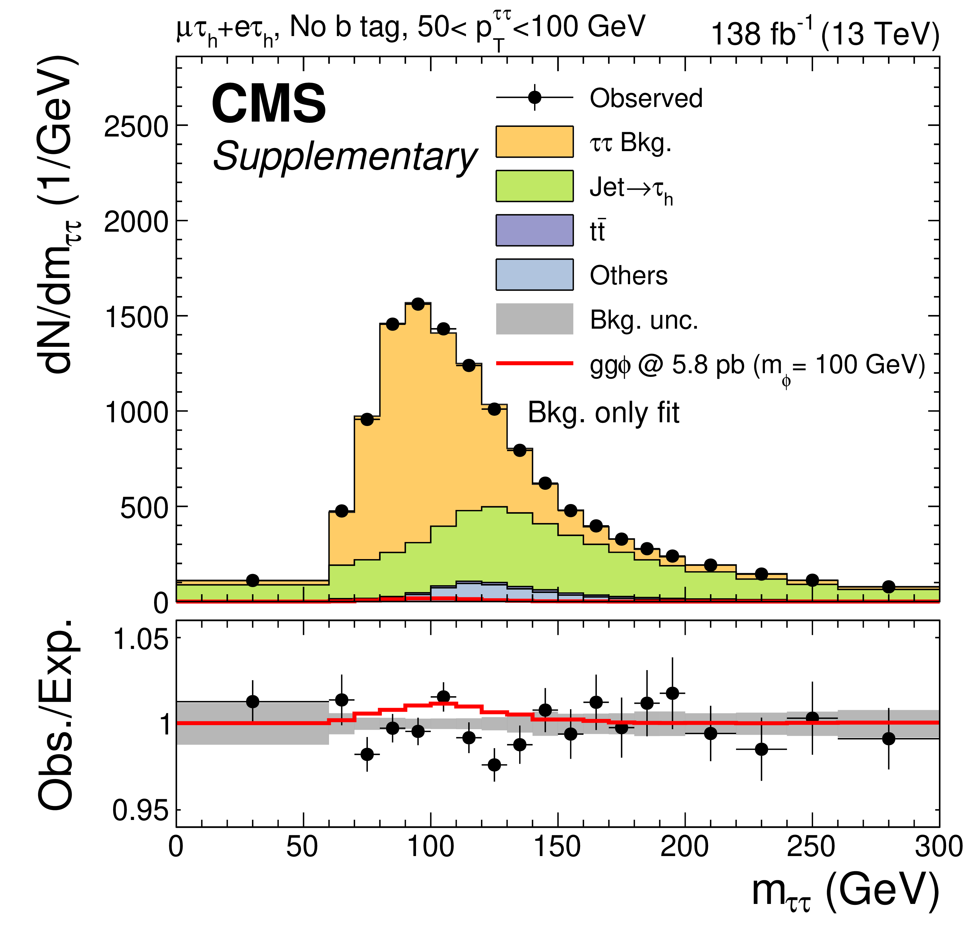
Additional Figure 6:
Distribution of $m_{ \tau \tau }$ in the ``No b tag, 50 $ < p_{\mathrm{T}} ^{ \tau \tau }< $ 100 GeV'' category used for the model-independent $\phi$ search for $m_{\phi}< $ 250 GeV, in the $ \mathrm{e} \tau _{\mathrm{h}}$ and $ \mu \tau _{\mathrm{h}}$ final states combined. The solid histograms show the stacked background predictions after a fit of the signal-plus-background hypothesis with $m_{\phi}= $ 100 GeV to the data. The best fit $ \mathrm{g} \mathrm{g} \phi$ signal is shown by the solid red line. The total background prediction estimated from a fit of the background-only hypothesis to the data is shown by the dashed blue line for comparison. The lower panel shows the ratio of the data over the background expectation after the fit of the signal-plus-background hypothesis to the data. The full predictions of the fits of the signal-plus-background (with signal) and background-only hypotheses are also shown by the solid red and dashed blue line, respectively. |
png pdf |
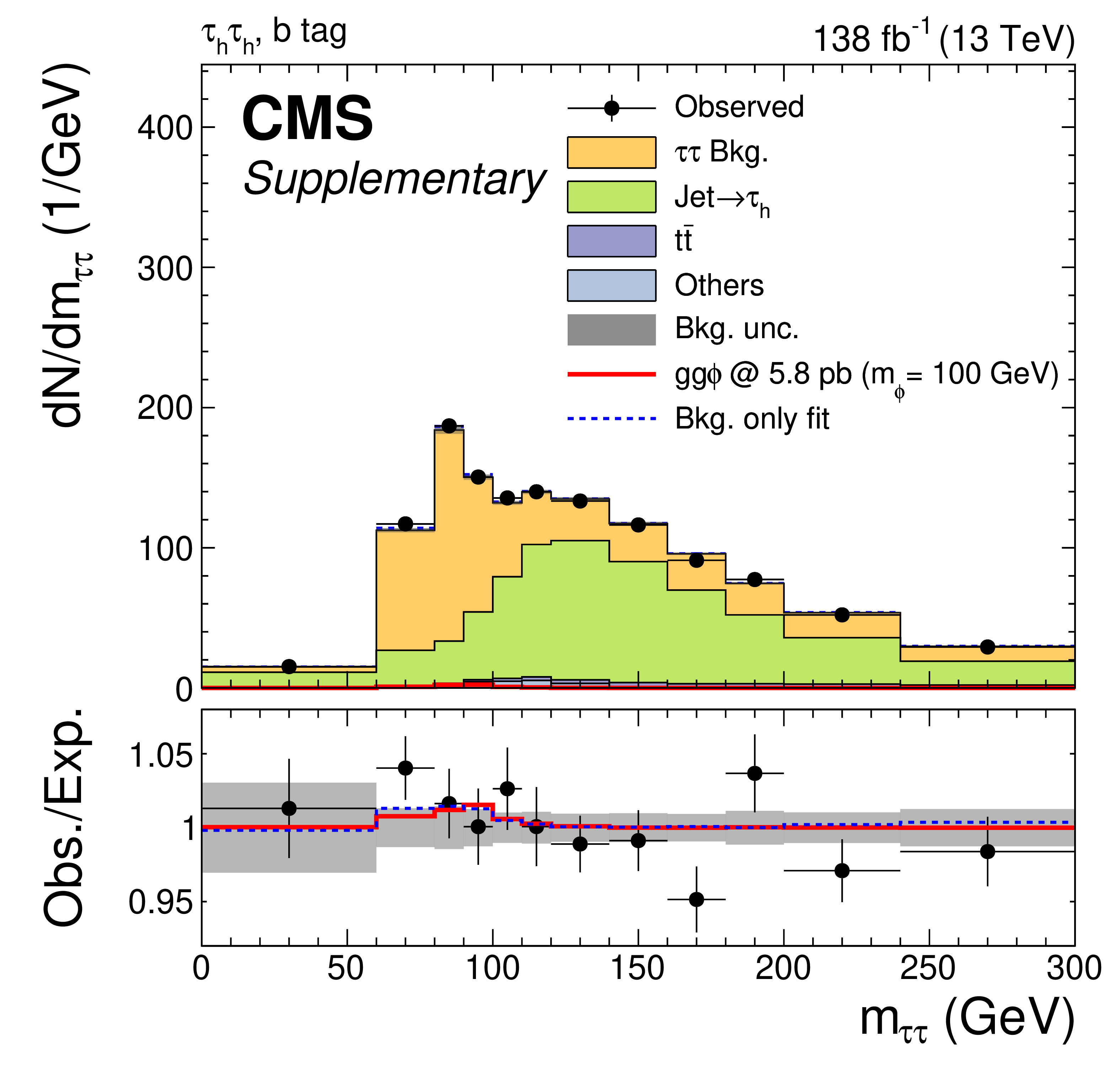
Additional Figure 7:
Distribution of $m_{ \tau \tau }$ in the ``b tag'' category used for the model-independent $\phi$ search for $m_{\phi}< $ 250 GeV, in the $ \tau _{\mathrm{h}} \tau _{\mathrm{h}}$ final state. The solid histograms show the stacked background predictions after a fit of the signal-plus-background hypothesis with $m_{\phi}= $ 100 GeV to the data. The best fit $ \mathrm{g} \mathrm{g} \phi$ signal is shown by the solid red line. The total background prediction estimated from a fit of the background-only hypothesis to the data is shown by the dashed blue line for comparison. The lower panel shows the ratio of the data over the background expectation after the fit of the signal-plus-background hypothesis to the data. The full predictions of the fits of the signal-plus-background (with signal) and background-only hypotheses are also shown by the solid red and dashed blue line, respectively. |
png pdf |
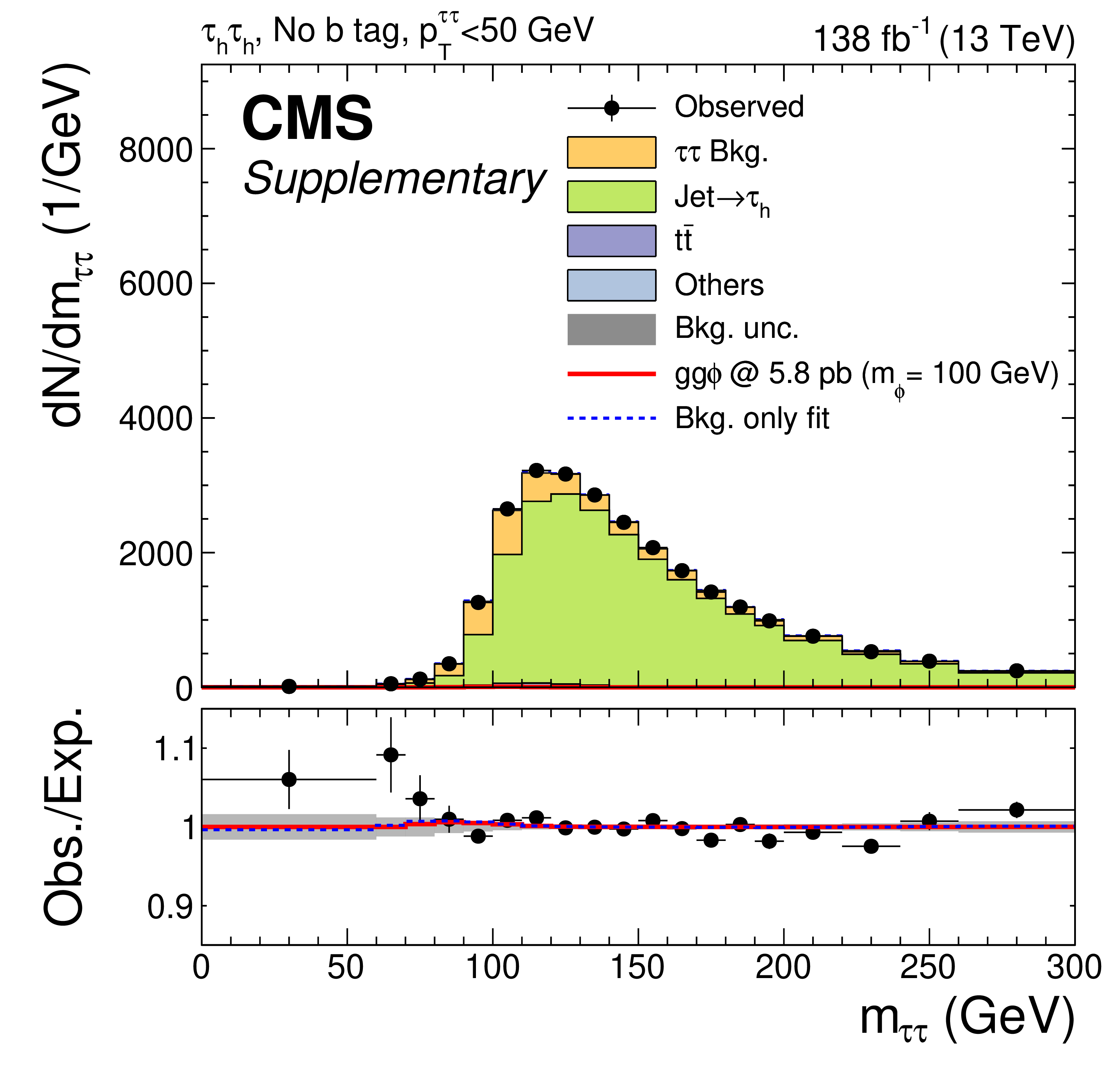
Additional Figure 8:
Distribution of $m_{ \tau \tau }$ in the ``No b tag, $ p_{\mathrm{T}} ^{ \tau \tau }< $ 50 GeV'' category used for the model-independent $\phi$ search for $m_{\phi}< $ 250 GeV, in the $ \tau _{\mathrm{h}} \tau _{\mathrm{h}}$ final state. The solid histograms show the stacked background predictions after a fit of the signal-plus-background hypothesis with $m_{\phi}= $ 100 GeV to the data. The best fit $ \mathrm{g} \mathrm{g} \phi$ signal is shown by the solid red line. The total background prediction estimated from a fit of the background-only hypothesis to the data is shown by the dashed blue line for comparison. The lower panel shows the ratio of the data over the background expectation after the fit of the signal-plus-background hypothesis to the data. The full predictions of the fits of the signal-plus-background (with signal) and background-only hypotheses are also shown by the solid red and dashed blue line, respectively. |
png pdf |
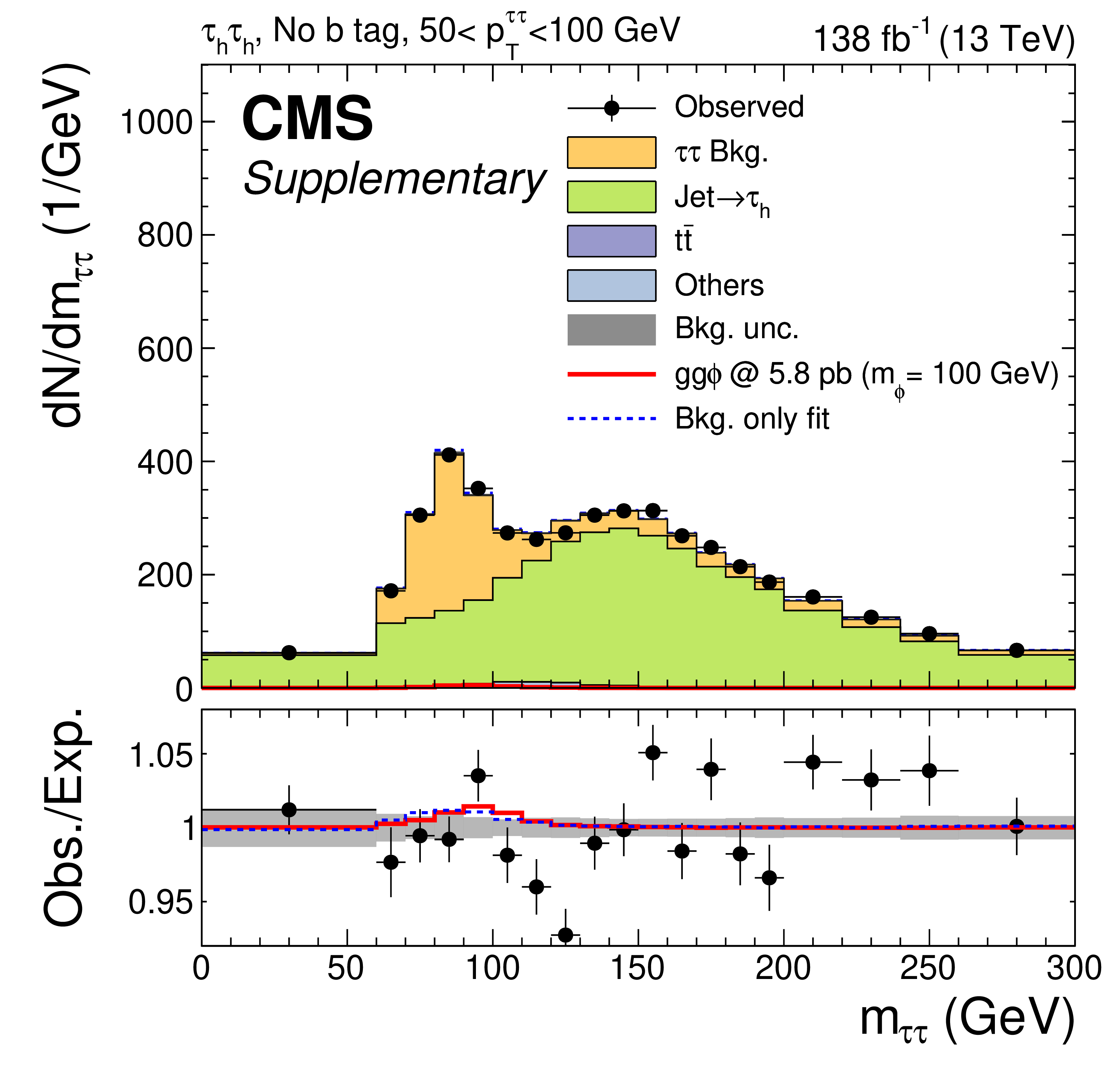
Additional Figure 9:
Distribution of $m_{ \tau \tau }$ in the ``No b tag, 50 $ < p_{\mathrm{T}} ^{ \tau \tau }< $ 100 GeV'' category used for the model-independent $\phi$ search for $m_{\phi}< $ 250 GeV, in the $ \tau _{\mathrm{h}} \tau _{\mathrm{h}}$ final state. The solid histograms show the stacked background predictions after a fit of the signal-plus-background hypothesis with $m_{\phi}= $ 100 GeV to the data. The best fit $ \mathrm{g} \mathrm{g} \phi$ signal is shown by the solid red line. The total background prediction estimated from a fit of the background-only hypothesis to the data is shown by the dashed blue line for comparison. The lower panel shows the ratio of the data over the background expectation after the fit of the signal-plus-background hypothesis to the data. The full predictions of the fits of the signal-plus-background (with signal) and background-only hypotheses are also shown by the solid red and dashed blue line, respectively. |
png pdf |
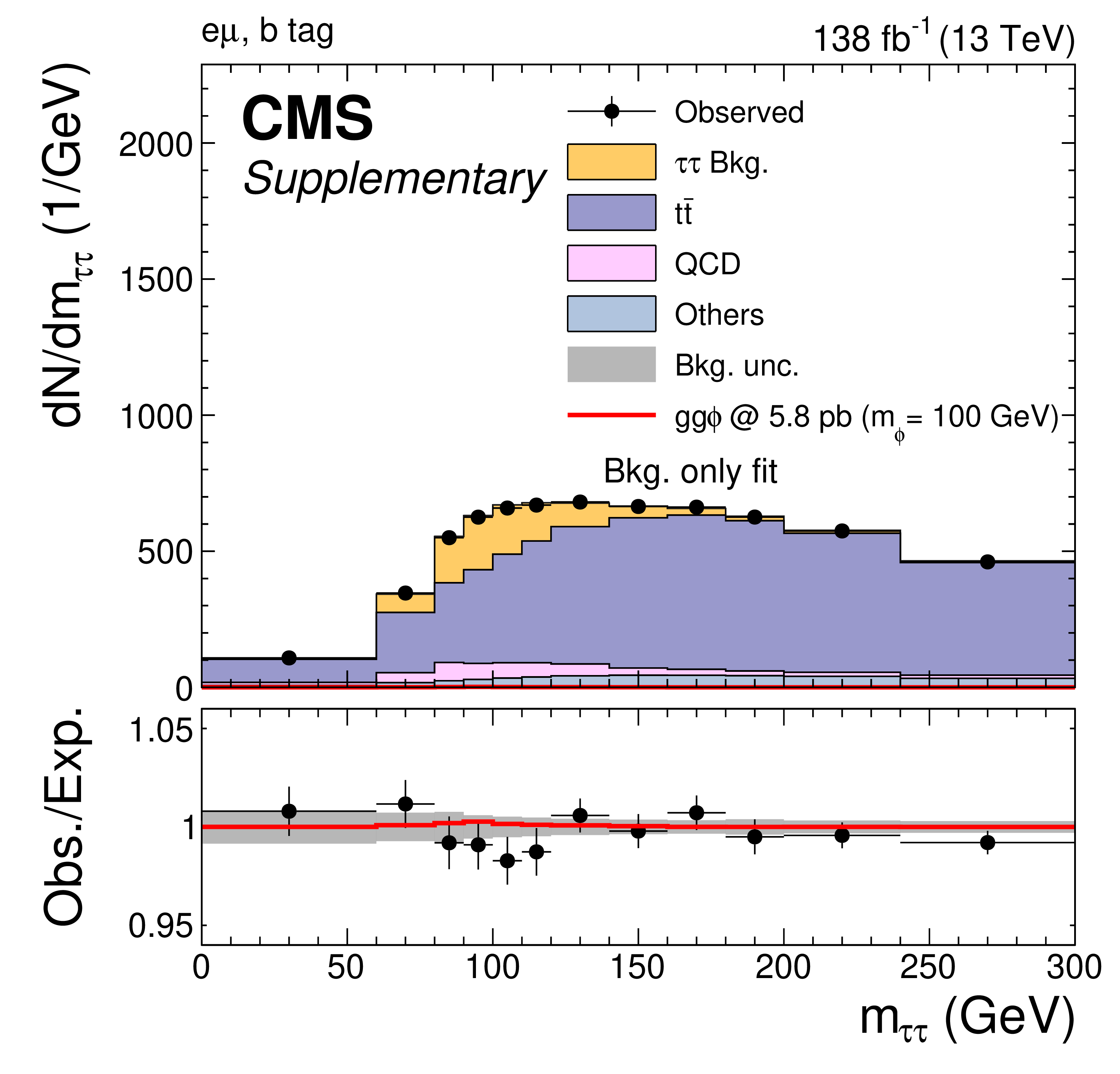
Additional Figure 10:
Distribution of $m_{ \tau \tau }$ in the ``b tag'' category used for the model-independent $\phi$ search for $m_{\phi}< $ 250 GeV, in the $ \mathrm{e} \mu $ final state, after a fit of the background-only hypothesis to the data. A $ \mathrm{g} \mathrm{g} \phi$ signal with $m_{\phi}= $ 100 GeV and a cross section of 5.8 pb is also shown, for illustrative purposes. |
png pdf |
Additional Figure 11:
Distribution of $m_{ \tau \tau }$ in the ``No b tag, $ p_{\mathrm{T}} ^{ \tau \tau }< $ 50 GeV'' category used for the model-independent $\phi$ search for $m_{\phi}\geq $ 250 GeV, in the $ \mathrm{e} \mu $ final state, after a fit of the background-only hypothesis to the data. A $ \mathrm{g} \mathrm{g} \phi$ signal with $m_{\phi}= $ 100 GeV and a cross section of 5.8 pb is also shown, for illustrative purposes. |
png pdf |
Additional Figure 12:
Distribution of $m_{ \tau \tau }$ in the ``No b tag, 50 $ < p_{\mathrm{T}} ^{ \tau \tau }< $ 100 GeV'' category used for the model-independent $\phi$ search for $m_{\phi}< $ 250 GeV, in the $ \mathrm{e} \mu $ final state, after a fit of the background-only hypothesis to the data. A $ \mathrm{g} \mathrm{g} \phi$ signal with $m_{\phi}= $ 100 GeV and a cross section of 5.8 pb is also shown, for illustrative purposes. |
png pdf |
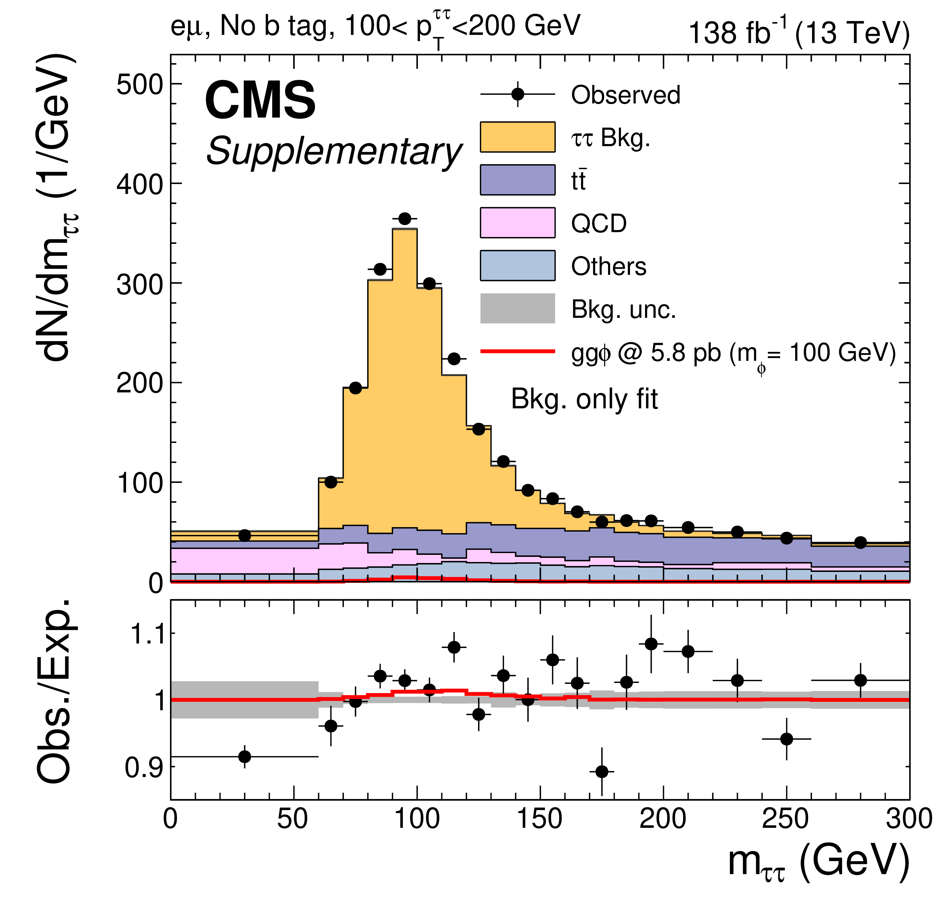
Additional Figure 13:
Distribution of $m_{ \tau \tau }$ in the ``No b tag, 100 $ < p_{\mathrm{T}} ^{ \tau \tau }< $ 200 GeV'' category used for the model-independent $\phi$ search for $m_{\phi}< $ 250 GeV, in the $ \mathrm{e} \mu $ final state, after a fit of the background-only hypothesis to the data. A $ \mathrm{g} \mathrm{g} \phi$ signal with $m_{\phi}= $ 100 GeV and a cross section of 5.8 pb is also shown, for illustrative purposes. |
png pdf |
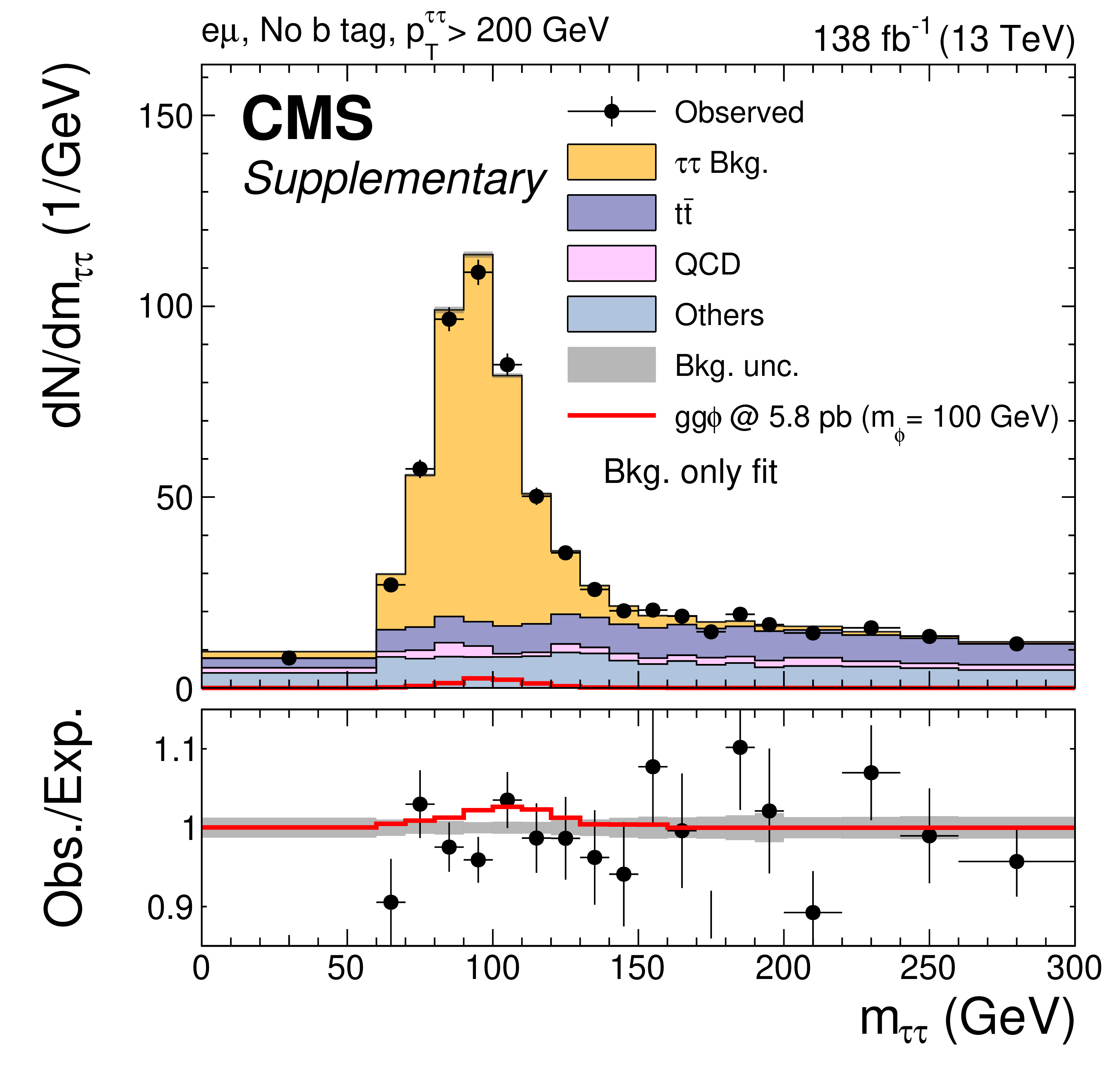
Additional Figure 14:
Distribution of $m_{ \tau \tau }$ in the ``No b tag, $ p_{\mathrm{T}} ^{ \tau \tau }> $ 200 GeV'' category used for the model-independent $\phi$ search for $m_{\phi}< $ 250 GeV, in the $ \mathrm{e} \mu $ final state, after a fit of the background-only hypothesis to the data. A $ \mathrm{g} \mathrm{g} \phi$ signal with $m_{\phi}= $ 100 GeV and a cross section of 5.8 pb is also shown, for illustrative purposes. |
png pdf |
Additional Figure 15:
Distribution of $m_{ \tau \tau }$ in the ``b tag'' category used for the model-independent $\phi$ search for $m_{\phi}< $ 250 GeV, in the $ \mathrm{e} \tau _{\mathrm{h}}$ and $ \mu \tau _{\mathrm{h}}$ final states combined, after a fit of the background-only hypothesis to the data. A $ \mathrm{g} \mathrm{g} \phi$ signal with $m_{\phi}= $ 100 GeV and a cross section of 5.8 pb is also shown, for illustrative purposes. |
png pdf |
Additional Figure 16:
Distribution of $m_{ \tau \tau }$ in the ``No b tag, $ p_{\mathrm{T}} ^{ \tau \tau }< $ 50 GeV'' category used for the model-independent $\phi$ search for $m_{\phi}< $ 250 GeV, in the $ \mathrm{e} \tau _{\mathrm{h}}$ and $ \mu \tau _{\mathrm{h}}$ final states combined, after a fit of the background-only hypothesis to the data. A $ \mathrm{g} \mathrm{g} \phi$ signal with $m_{\phi}= $ 100 GeV and a cross section of 5.8 pb is also shown, for illustrative purposes. |
png pdf |
Additional Figure 17:
Distribution of $m_{ \tau \tau }$ in the ``No b tag, 50 $ < p_{\mathrm{T}} ^{ \tau \tau }< $ 100 GeV'' category used for the model-independent $\phi$ search for $m_{\phi}< $ 250 GeV, in the $ \mathrm{e} \tau _{\mathrm{h}}$ and $ \mu \tau _{\mathrm{h}}$ final states combined, after a fit of the background-only hypothesis to the data. A $ \mathrm{g} \mathrm{g} \phi$ signal with $m_{\phi}= $ 100 GeV and a cross section of 5.8 pb is also shown, for illustrative purposes. |
png pdf |
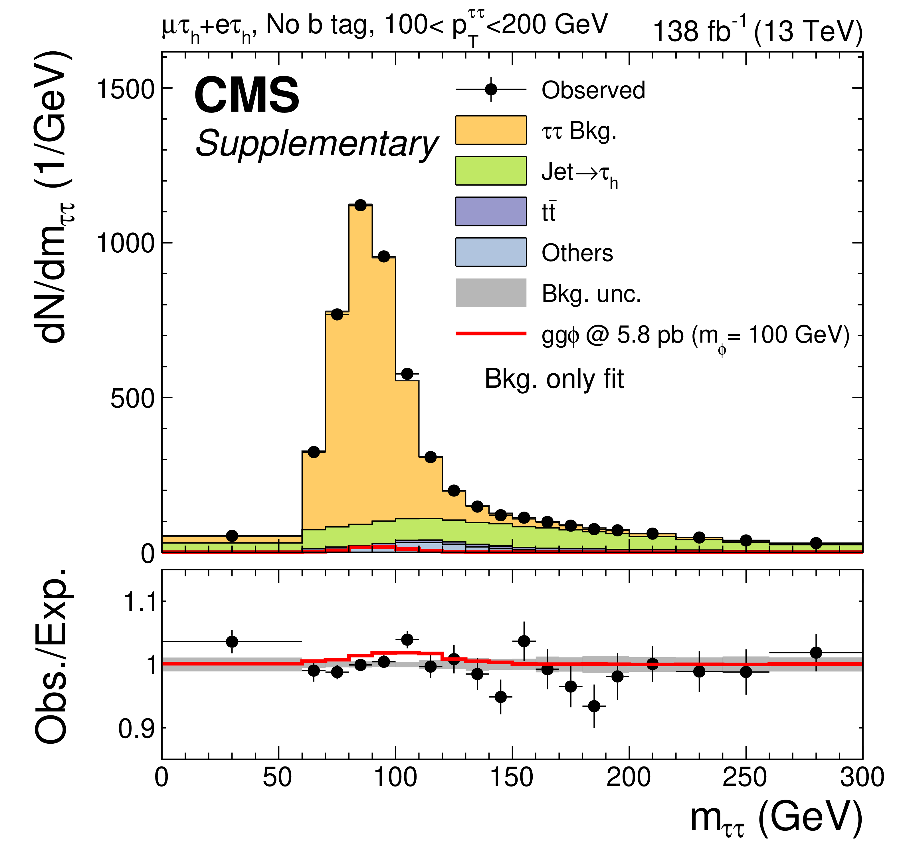
Additional Figure 18:
Distribution of $m_{ \tau \tau }$ in the ``No b tag, 100 $ < p_{\mathrm{T}} ^{ \tau \tau }< $ 200 GeV'' category used for the model-independent $\phi$ search for $m_{\phi}< $ 250 GeV, in the $ \mathrm{e} \tau _{\mathrm{h}}$ and $ \mu \tau _{\mathrm{h}}$ final states combined, after a fit of the background-only hypothesis to the data. A $ \mathrm{g} \mathrm{g} \phi$ signal with $m_{\phi}= $ 100 GeV and a cross section of 5.8 pb is also shown, for illustrative purposes. |

png pdf |
Additional Figure 19:
Distribution of $m_{ \tau \tau }$ in the ``No b tag, $ p_{\mathrm{T}} ^{ \tau \tau }> $ 200 GeV'' category used for the model-independent $\phi$ search for $m_{\phi}< $ 250 GeV, in the $ \mathrm{e} \tau _{\mathrm{h}}$ and $ \mu \tau _{\mathrm{h}}$ final states combined, after a fit of the background-only hypothesis to the data. A $ \mathrm{g} \mathrm{g} \phi$ signal with $m_{\phi}= $ 100 GeV and a cross section of 5.8 pb is also shown, for illustrative purposes. |

png pdf |
Additional Figure 20:
Distribution of $m_{ \tau \tau }$ in the ``b tag'' category used for the model-independent $\phi$ search for $m_{\phi}< $ 250 GeV, in the $ \tau _{\mathrm{h}} \tau _{\mathrm{h}}$ final state, after a fit of the background-only hypothesis to the data. A $ \mathrm{g} \mathrm{g} \phi$ signal with $m_{\phi}= $ 100 GeV and a cross section of 5.8 pb is also shown, for illustrative purposes. |
png pdf |
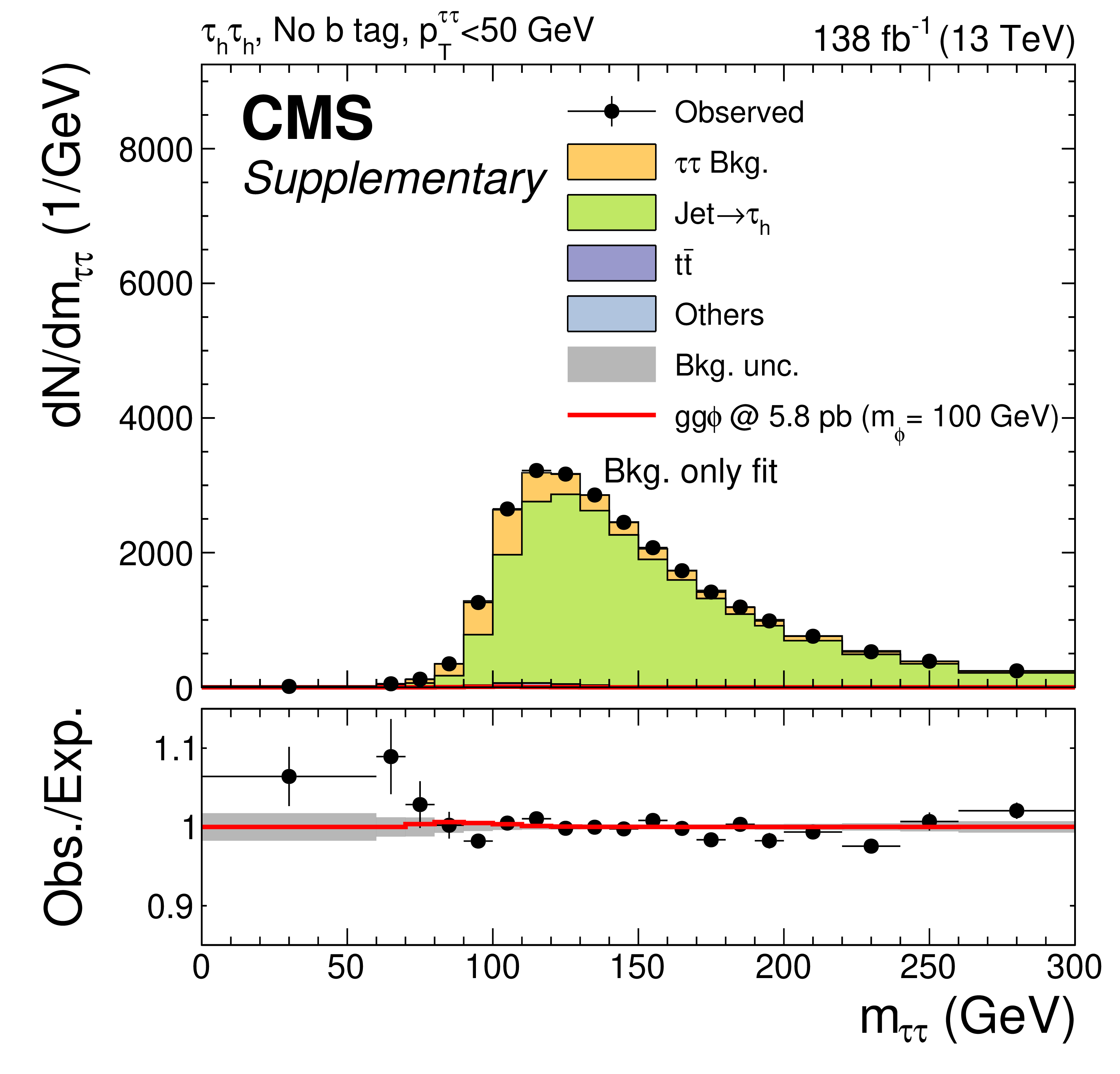
Additional Figure 21:
Distribution of $m_{ \tau \tau }$ in the ``No b tag, $ p_{\mathrm{T}} ^{ \tau \tau }< $ 50 GeV'' category used for the model-independent $\phi$ search for $m_{\phi}< $ 250 GeV, in the $ \tau _{\mathrm{h}} \tau _{\mathrm{h}}$ final state, after a fit of the background-only hypothesis to the data. A $ \mathrm{g} \mathrm{g} \phi$ signal with $m_{\phi}= $ 100 GeV and a cross section of 5.8 pb is also shown, for illustrative purposes. |
png pdf |
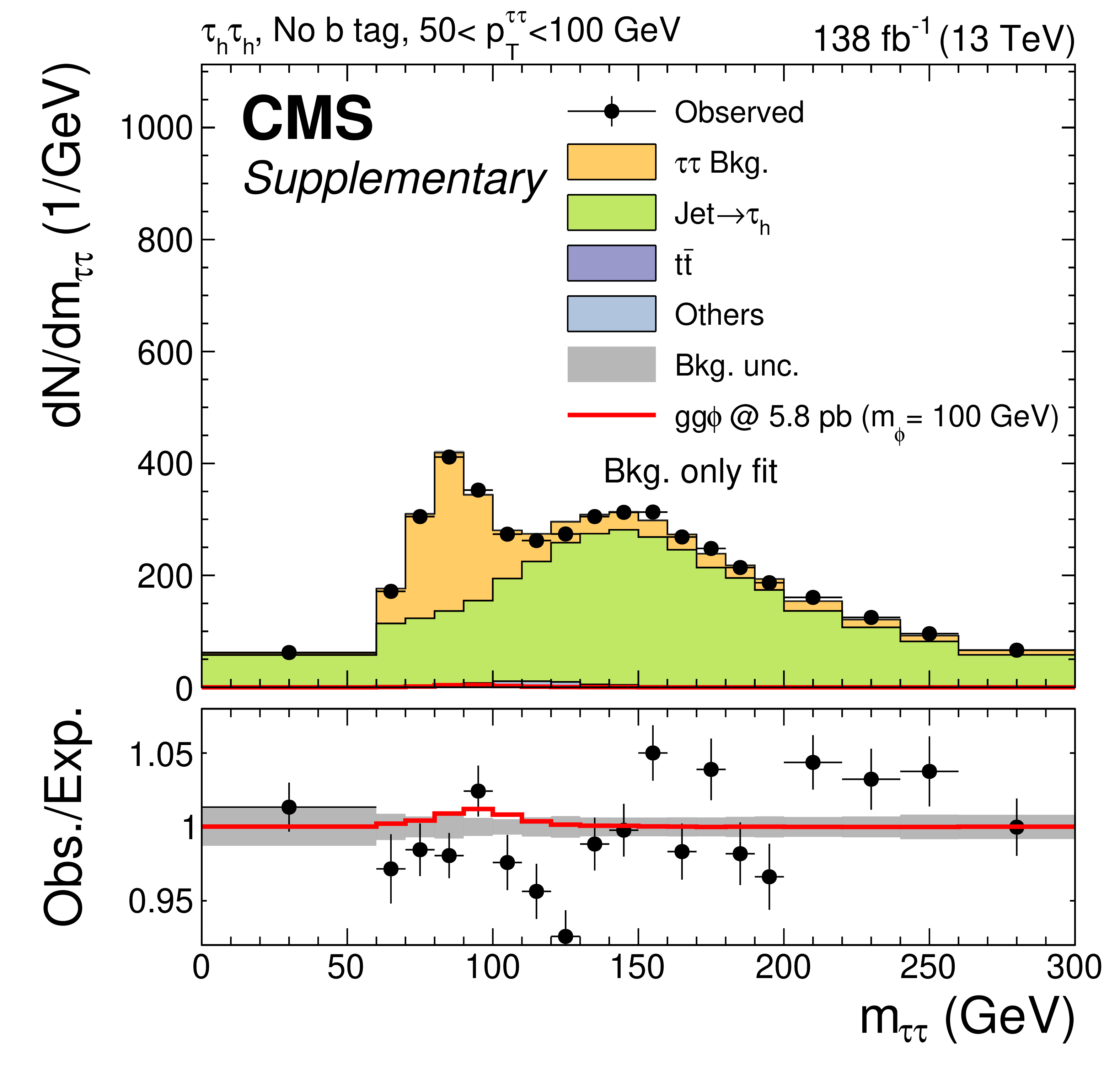
Additional Figure 22:
Distribution of $m_{ \tau \tau }$ in the ``No b tag, 50 $ < p_{\mathrm{T}} ^{ \tau \tau }< $ 100 GeV'' category used for the model-independent $\phi$ search for $m_{\phi}< $ 250 GeV, in the $ \tau _{\mathrm{h}} \tau _{\mathrm{h}}$ final state, after a fit of the background-only hypothesis to the data. A $ \mathrm{g} \mathrm{g} \phi$ signal with $m_{\phi}= $ 100 GeV and a cross section of 5.8 pb is also shown, for illustrative purposes. |
png pdf |
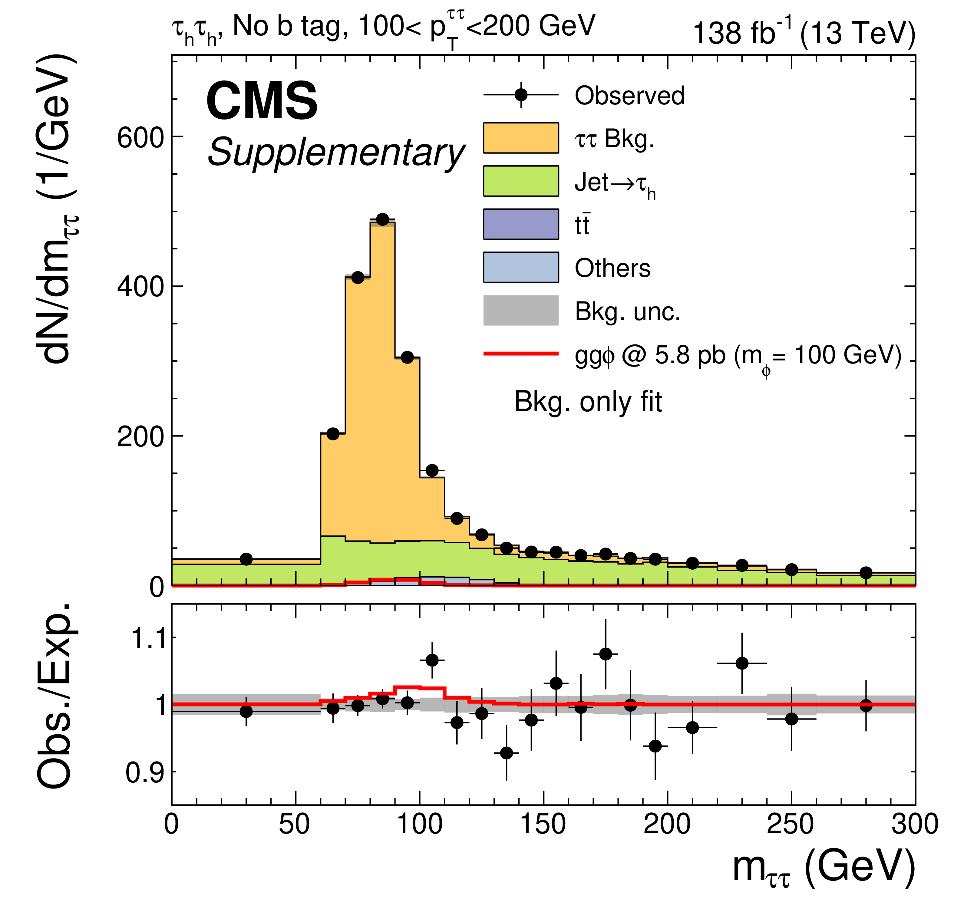
Additional Figure 23:
Distribution of $m_{ \tau \tau }$ in the ``No b tag, 100 $ < p_{\mathrm{T}} ^{ \tau \tau }< $ 200 GeV'' category used for the model-independent $\phi$ search for $m_{\phi}< $ 250 GeV, in the $ \tau _{\mathrm{h}} \tau _{\mathrm{h}}$ final state, after a fit of the background-only hypothesis to the data. A $ \mathrm{g} \mathrm{g} \phi$ signal with $m_{\phi}= $ 100 GeV and a cross section of 5.8 pb is also shown, for illustrative purposes. |
png pdf |
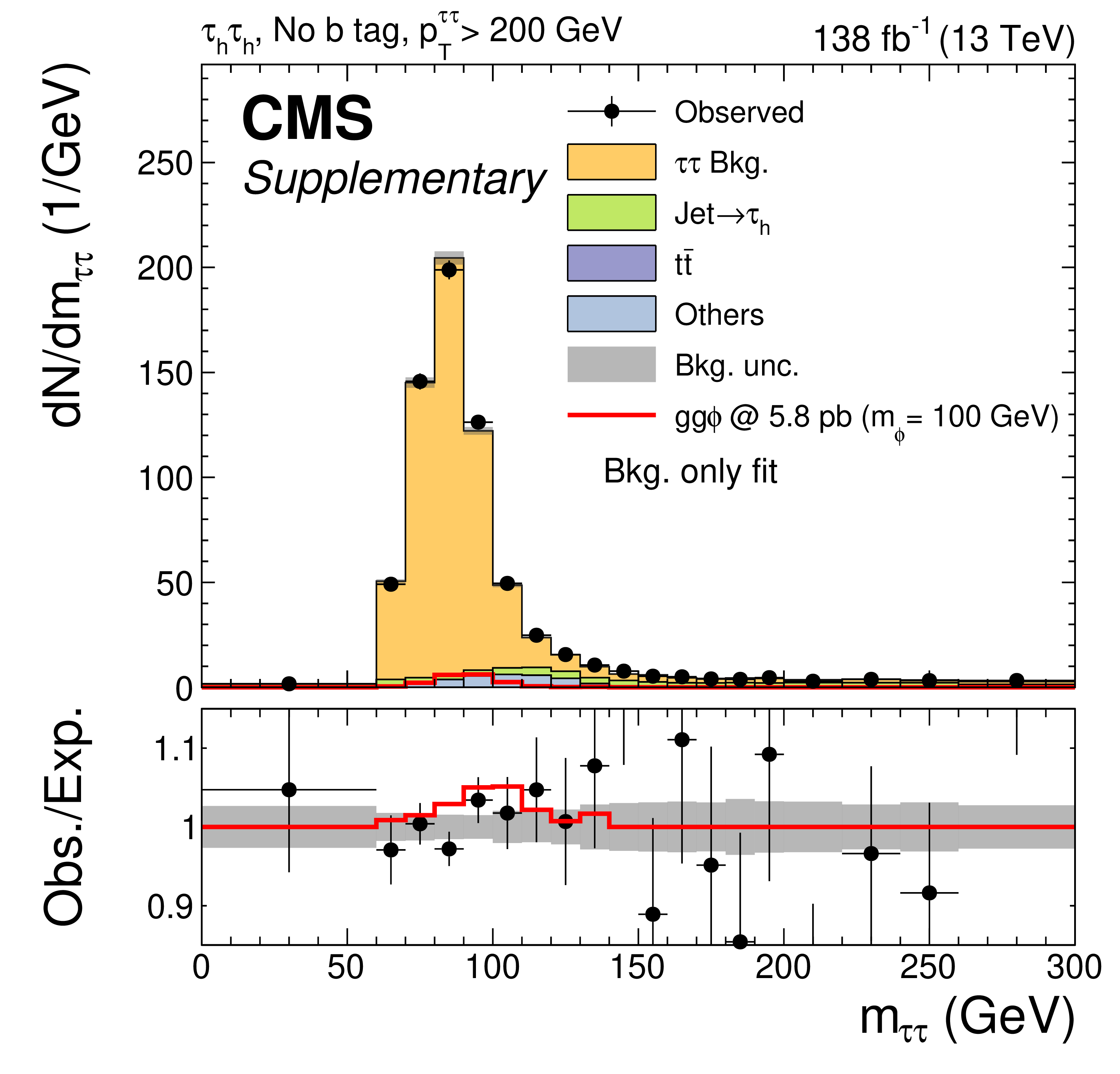
Additional Figure 24:
Distribution of $m_{ \tau \tau }$ in the ``No b tag, $ p_{\mathrm{T}} ^{ \tau \tau }> $ 200 GeV'' category used for the model-independent $\phi$ search in the $ \tau _{\mathrm{h}} \tau _{\mathrm{h}}$ final state, after a fit of the background-only hypothesis to the data. A $ \mathrm{g} \mathrm{g} \phi$ signal with $m_{\phi}= $ 100 GeV and a cross section of 5.8 pb is also shown, for illustrative purposes. |
png pdf |
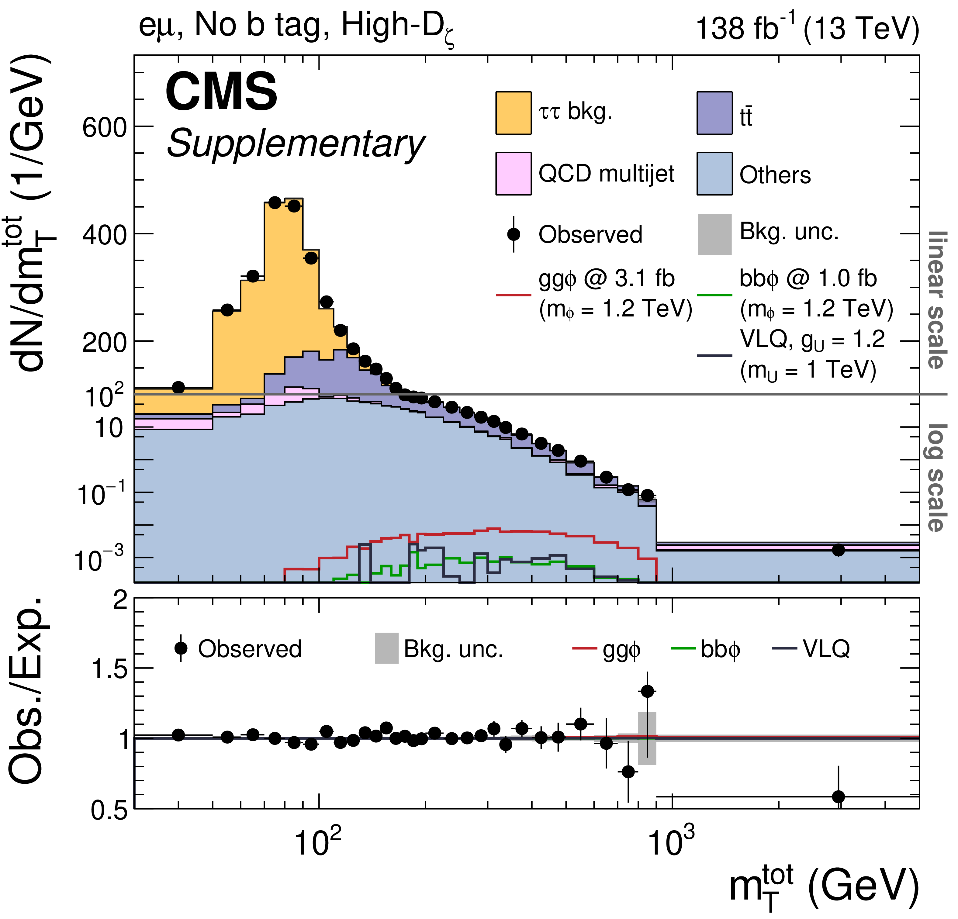
Additional Figure 25:
Distribution of $m_{\text{T}}^{\text{tot}}$ in the ``No b tag, High-$D_{\zeta}$'' category used for the model-independent $\phi$ search for $m_{\phi}\geq $ 250 GeV, the search for vector leptoquarks, and the interpretation in MSSM benchmark scenarios, in the $ \mathrm{e} \mu $ final state. The background model is shown after the fit of the background-only hypothesis to the data. A $ \mathrm{g} \mathrm{g} \phi$ and $ \mathrm{b} \mathrm{b} \phi$ signal with $m_{\phi} = $ 1.2 TeV scaled to 3.1 and 1.0 fb, and a vector leptoquark signal with $m_{\text{U}}= $ 1 TeV and $g_{\text{U}}= $ 1.2 are also shown for illustrative purposes. |
png pdf |
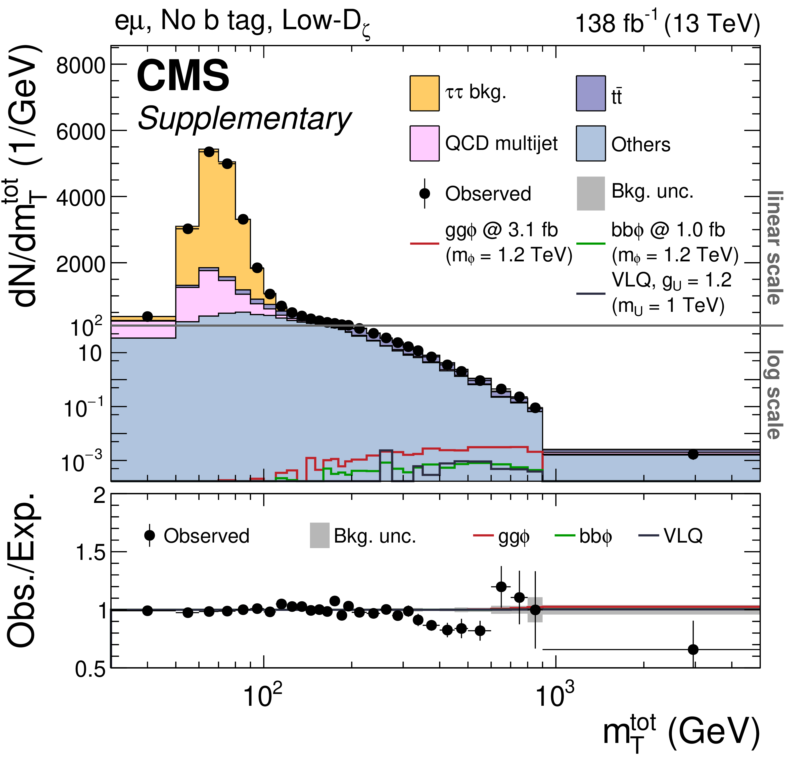
Additional Figure 26:
Distribution of $m_{\text{T}}^{\text{tot}}$ in the ``No b tag, Low-$D_{\zeta}$'' category used for the model-independent $\phi$ search for $m_{\phi}\geq $ 250 GeV, the search for vector leptoquarks, and the interpretation in MSSM benchmark scenarios, in the $ \mathrm{e} \mu $ final state. The background model is shown after the fit of the background-only hypothesis to the data. A $ \mathrm{g} \mathrm{g} \phi$ and $ \mathrm{b} \mathrm{b} \phi$ signal with $m_{\phi} = $ 1.2 TeV scaled to 3.1 and 1.0 fb, and a vector leptoquark signal with $m_{\text{U}}= $ 1 TeV and $g_{\text{U}}= $ 1.2 are also shown for illustrative purposes. |
png pdf |
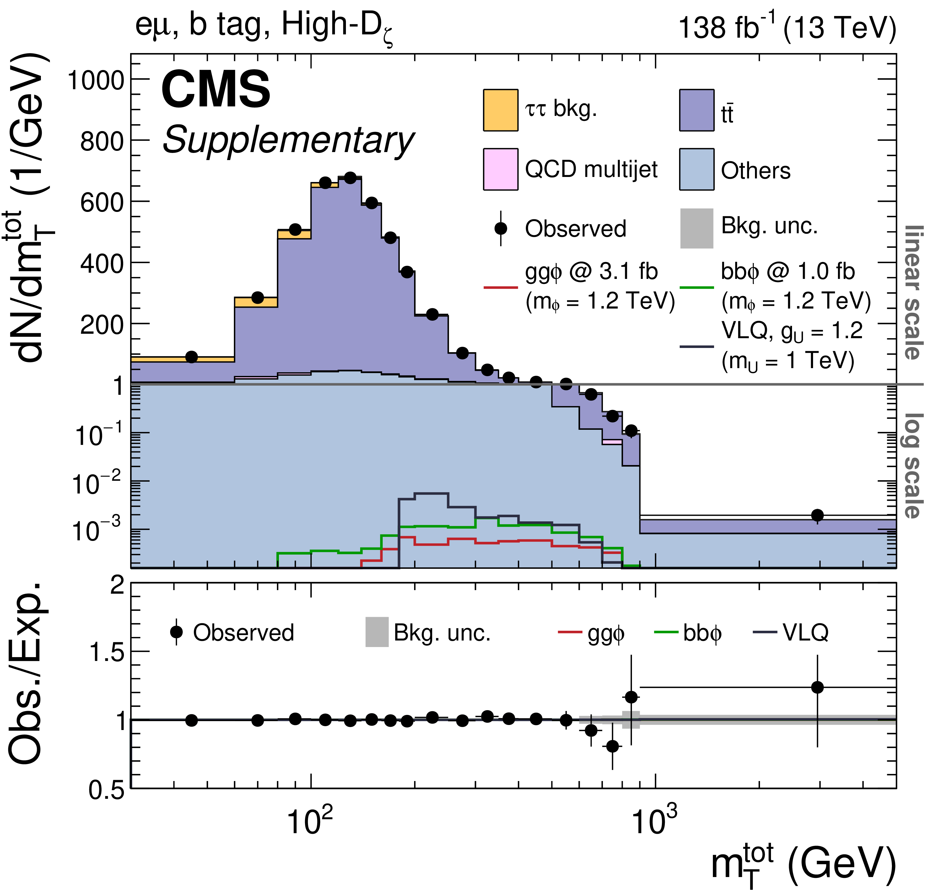
Additional Figure 27:
Distribution of $m_{\text{T}}^{\text{tot}}$ in the ``b tag, High-$D_{\zeta}$'' category used for the model-independent $\phi$ search for $m_{\phi}\geq $ 250 GeV, the search for vector leptoquarks, and the interpretation in MSSM benchmark scenarios, in the $ \mathrm{e} \mu $ final state. The background model is shown after the fit of the background-only hypothesis to the data. A $ \mathrm{g} \mathrm{g} \phi$ and $ \mathrm{b} \mathrm{b} \phi$ signal with $m_{\phi}= $ 1.2 TeV scaled to 3.1 and 1.0 fb, and a vector leptoquark signal with $m_{\text{U}}= $ 1 TeV and $g_{\text{U}}= $ 1.2 are also shown for illustrative purposes. |
png pdf |
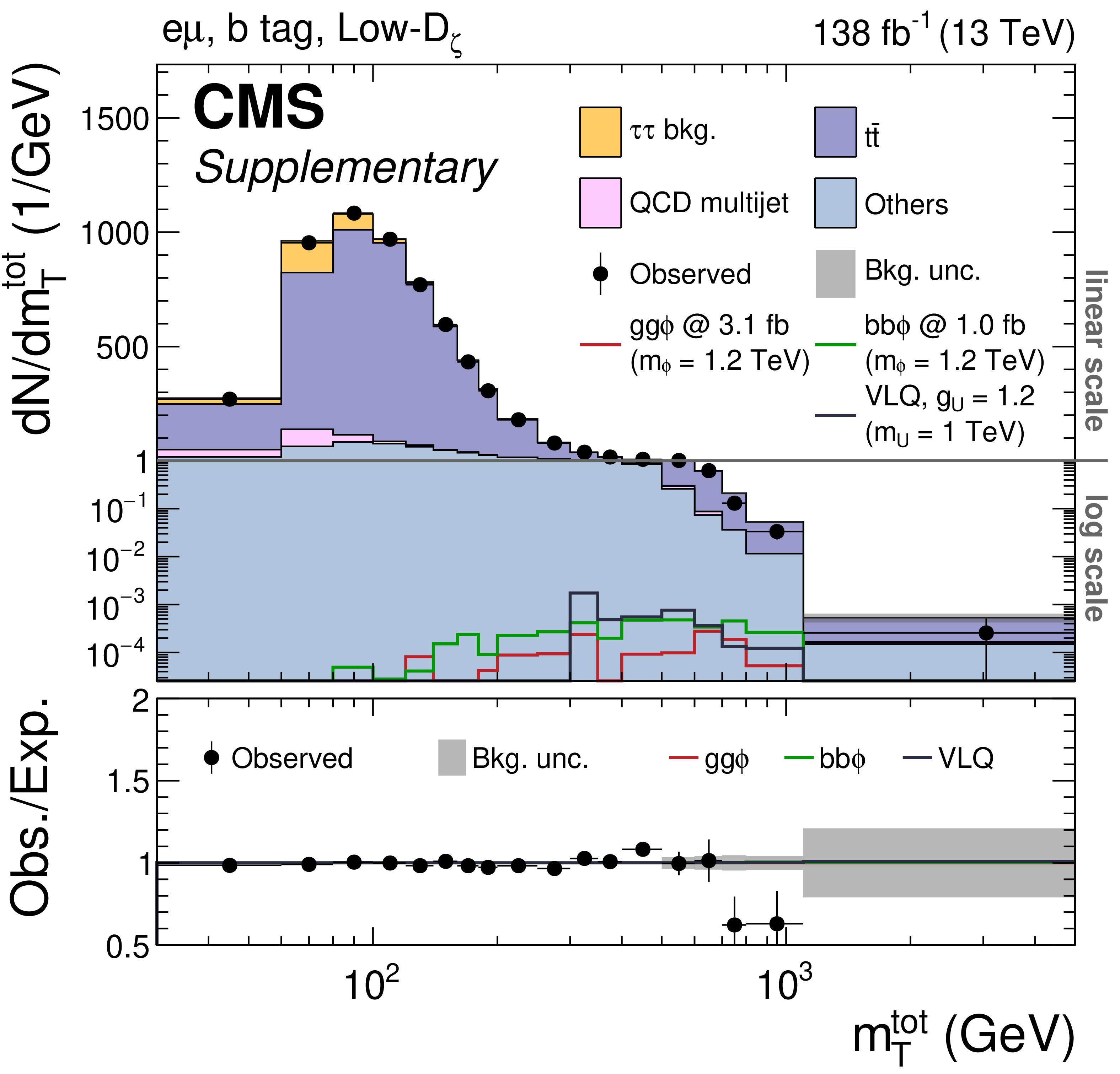
Additional Figure 28:
Distribution of $m_{\text{T}}^{\text{tot}}$ in the ``b tag, Low-$D_{\zeta}$'' category used for the model-independent $\phi$ search for $m_{\phi}\geq $ 250 GeV, the search for vector leptoquarks, and the interpretation in MSSM benchmark scenarios, in the $ \mathrm{e} \mu $ final state. The background model is shown after the fit of the background-only hypothesis to the data. A $ \mathrm{g} \mathrm{g} \phi$ and $ \mathrm{b} \mathrm{b} \phi$ signal with $m_{\phi}= $ 1.2 TeV scaled to 3.1 and 1.0 fb, and a vector leptoquark signal with $m_{\text{U}}= $ 1 TeV and $g_{\text{U}}= $ 1.2 are also shown for illustrative purposes. |
png pdf |
Additional Figure 29:
Distribution of $m_{\text{T}}^{\text{tot}}$ in the global ``No b tag, Loose-$ m_{\mathrm{T}} $'' category used for the model-independent $\phi$ search for $m_{\phi}\geq $ 250 GeV, the search for vector leptoquarks, and the interpretation in MSSM benchmark scenarios, in the $ \mathrm{e} \tau _{\mathrm{h}}$ and $ \mu \tau _{\mathrm{h}}$ final states combined. The background model is shown after the fit of the background-only hypothesis to the data. A $ \mathrm{g} \mathrm{g} \phi$ and $ \mathrm{b} \mathrm{b} \phi$ signal with $m_{\phi}= $ 1.2 TeV scaled to 3.1 and 1.0 fb, and a vector leptoquark signal with $m_{\text{U}}= $ 1 TeV and $g_{\text{U}}= $ 1.2 are also shown for illustrative purposes. |
png pdf |
Additional Figure 30:
Distribution of $m_{\text{T}}^{\text{tot}}$ in the ``b tag, Loose-$ m_{\mathrm{T}} $'' category used for the model-independent $\phi$ search for $m_{\phi}\geq $ 250 GeV, the search for vector leptoquarks, and the interpretation in MSSM benchmark scenarios, in the $ \mathrm{e} \tau _{\mathrm{h}}$ and $ \mu \tau _{\mathrm{h}}$ final states combined. The background model is shown after the fit of the background-only hypothesis to the data. A $ \mathrm{g} \mathrm{g} \phi$ and $ \mathrm{b} \mathrm{b} \phi$ signal with $m_{\phi}= $ 1.2 TeV scaled to 3.1 and 1.0 fb, and a vector leptoquark signal with $m_{\text{U}}= $ 1 TeV and $g_{\text{U}}= $ 1.2 are also shown for illustrative purposes. |
png pdf |
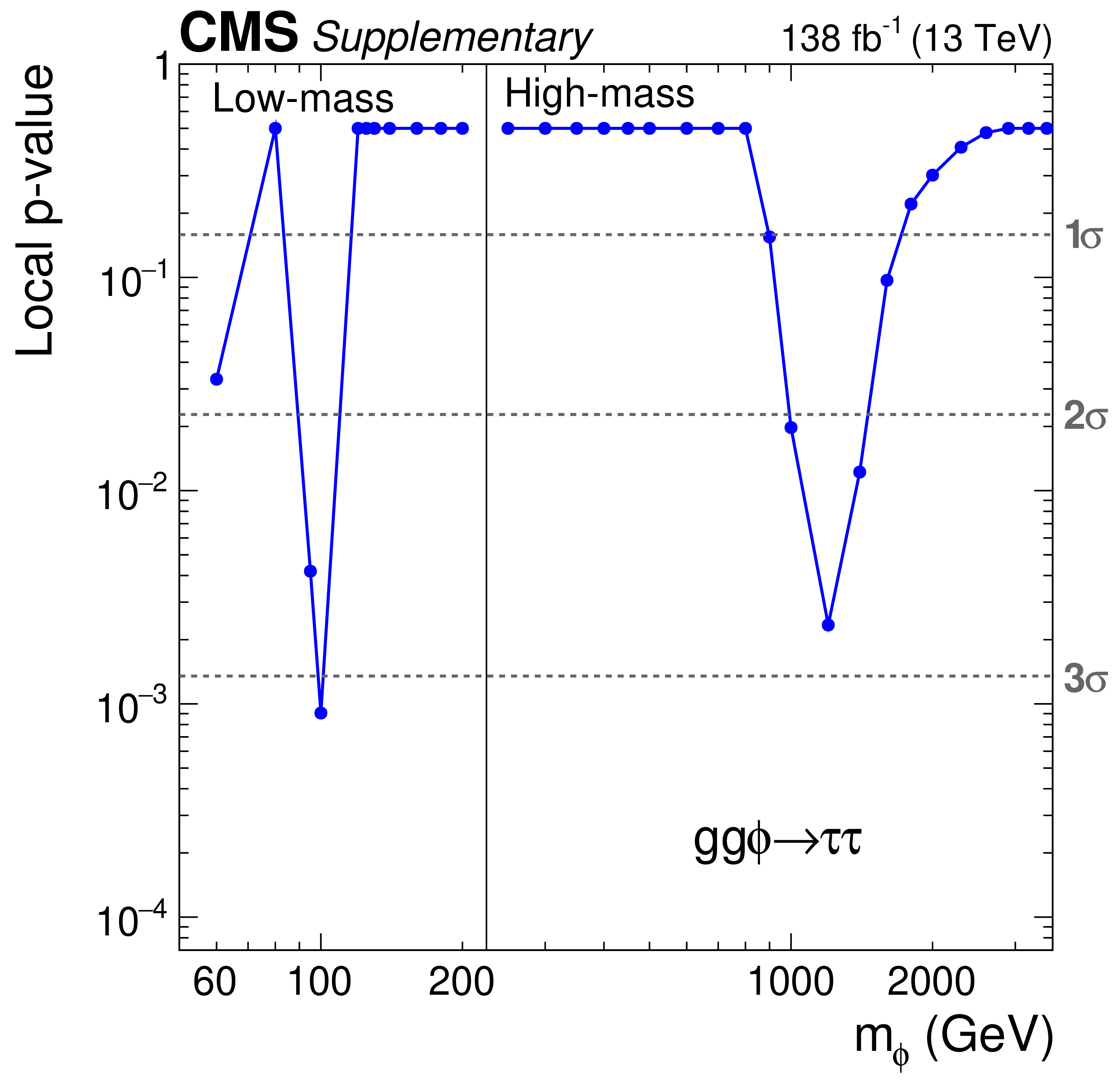
Additional Figure 31:
Local $p$-value and significance of a $ \mathrm{g} \mathrm{g} \phi$ signal as a function of the hypothesized value of $m_{\phi}$. For this figure the $ \mathrm{b} \mathrm{b} \phi$ production rate has been profiled. |
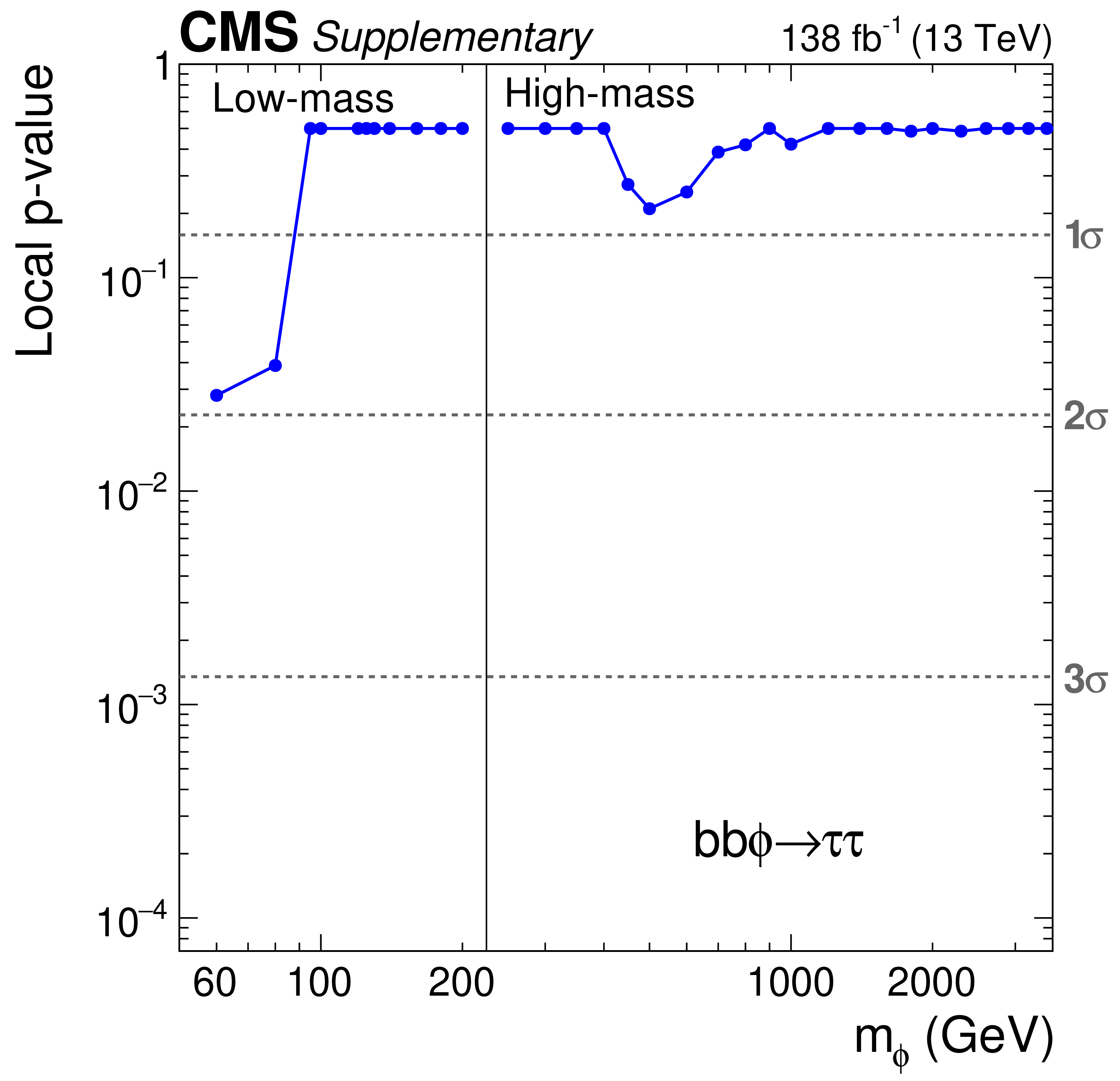
png pdf |
Additional Figure 32:
Local $p$-value and significance of a $ \mathrm{b} \mathrm{b} \phi$ signal as a function of the hypothesized value of $m_{\phi}$. For this figure the $ \mathrm{g} \mathrm{g} \phi$ production rate has been profiled. |
png pdf |
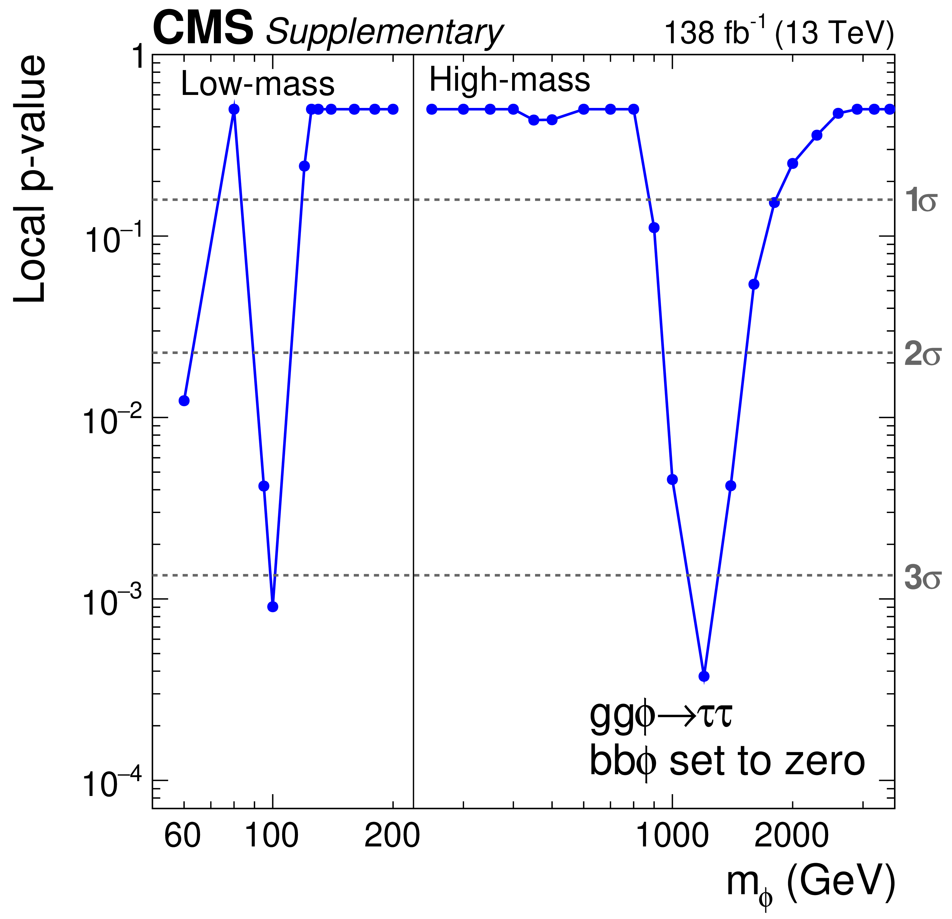
Additional Figure 33:
Local $p$-value and significance of a $ \mathrm{g} \mathrm{g} \phi$ signal as a function of the hypothesized value of $m_{\phi}$. For this figure the $ \mathrm{b} \mathrm{b} \phi$ production rate has been fixed to zero. |
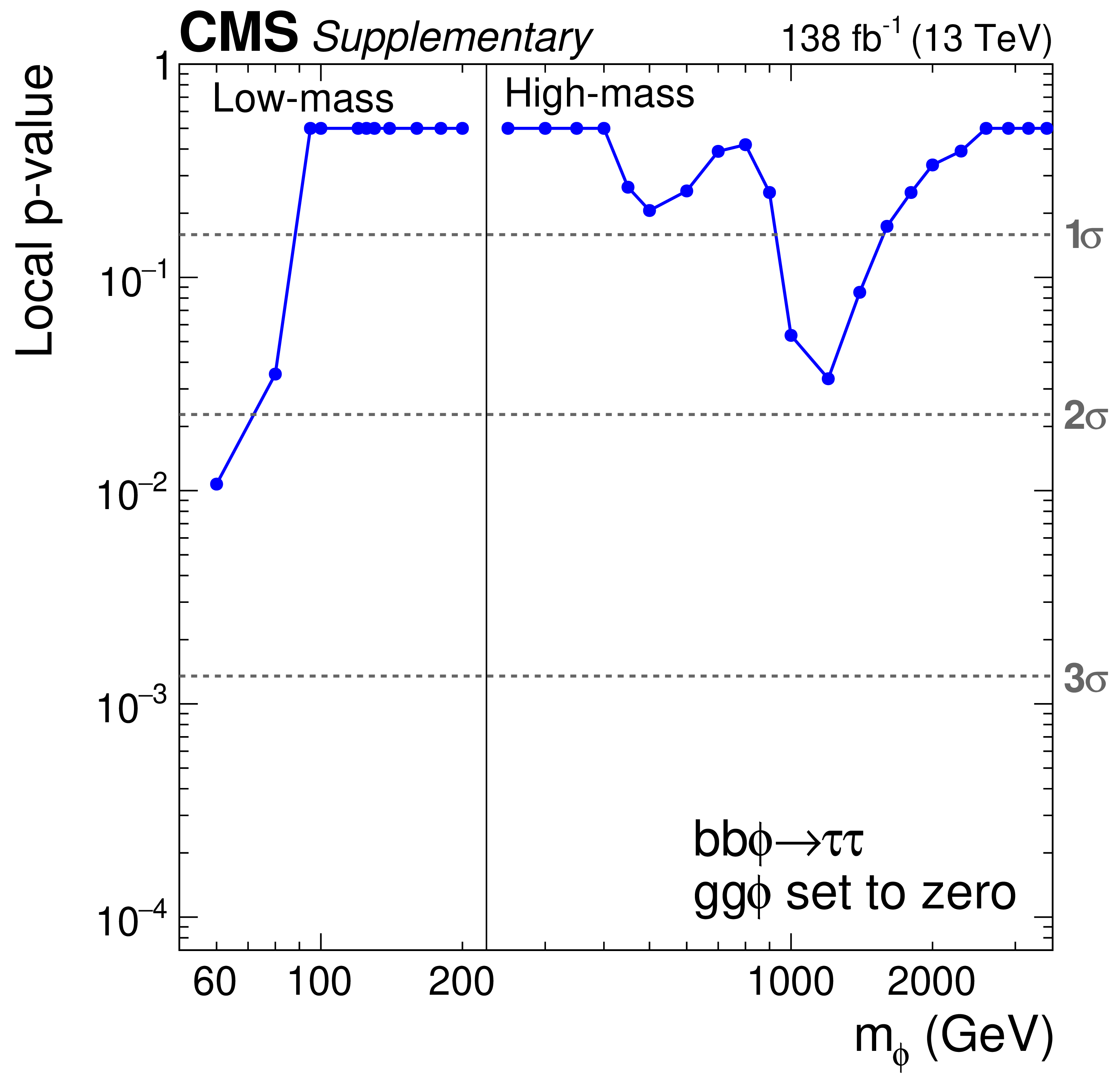
png pdf |
Additional Figure 34:
Local $p$-value and significance of a $ \mathrm{b} \mathrm{b} \phi$ signal as a function of the hypothesized value of $m_{\phi}$. For this figure the $ \mathrm{g} \mathrm{g} \phi$ production rate has been fixed to zero. |

png pdf |
Additional Figure 35:
Local $p$-value and significance of a $ \mathrm{g} \mathrm{g} \phi$ signal as a function of the hypothesized value of $m_{\phi}$. For this figure the $ \mathrm{b} \mathrm{b} \phi$ production rate has been profiled and only t quarks are considered in the $ \mathrm{g} \mathrm{g} \phi$ loop. |
png pdf |
Additional Figure 36:
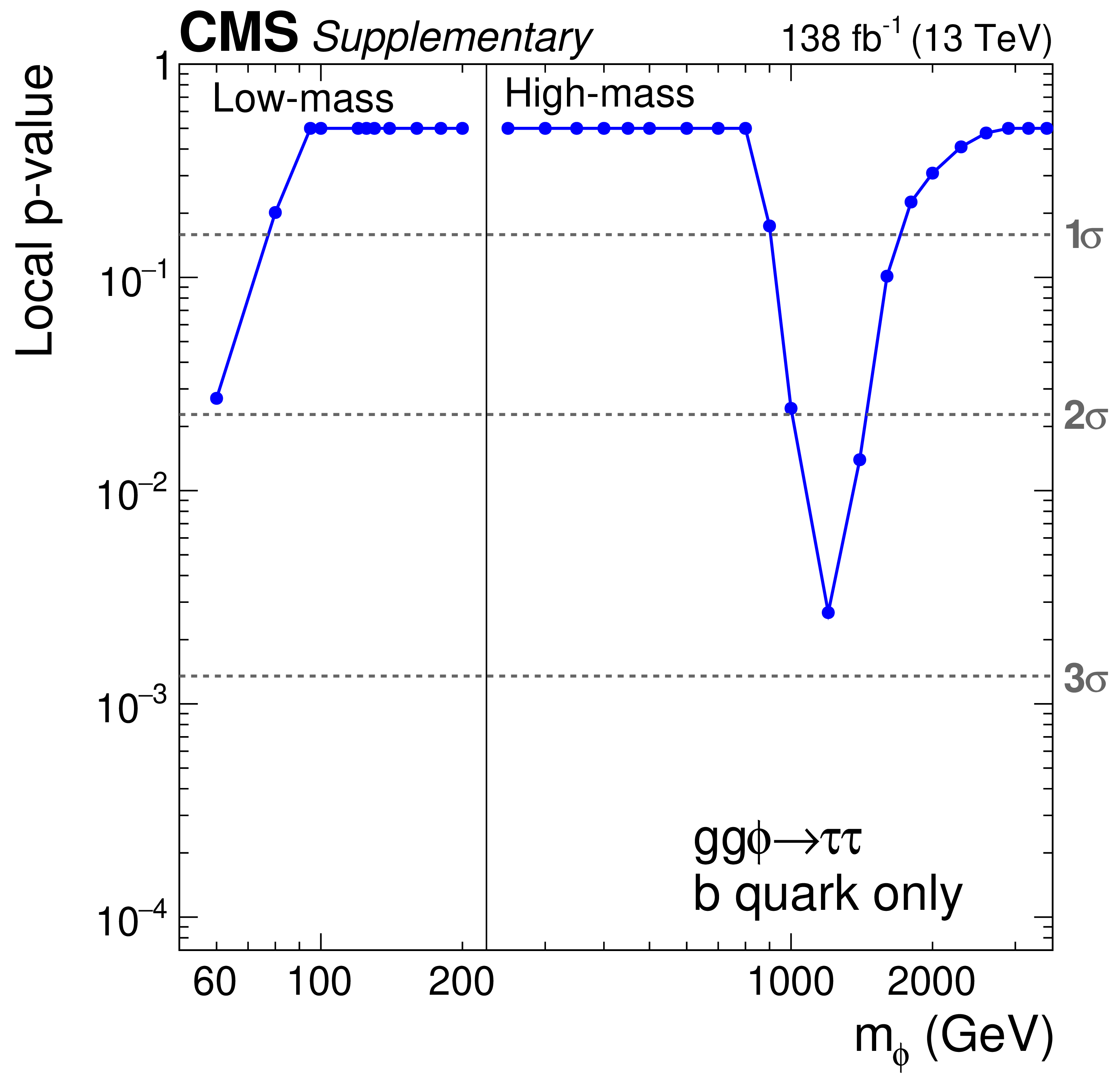
Local $p$-value and significance of a $ \mathrm{g} \mathrm{g} \phi$ signal as a function of the hypothesized value of $m_{\phi}$. For this figure the $ \mathrm{b} \mathrm{b} \phi$ production rate has been profiled and only b quarks are considered in the $ \mathrm{g} \mathrm{g} \phi$ loop. |
png pdf |
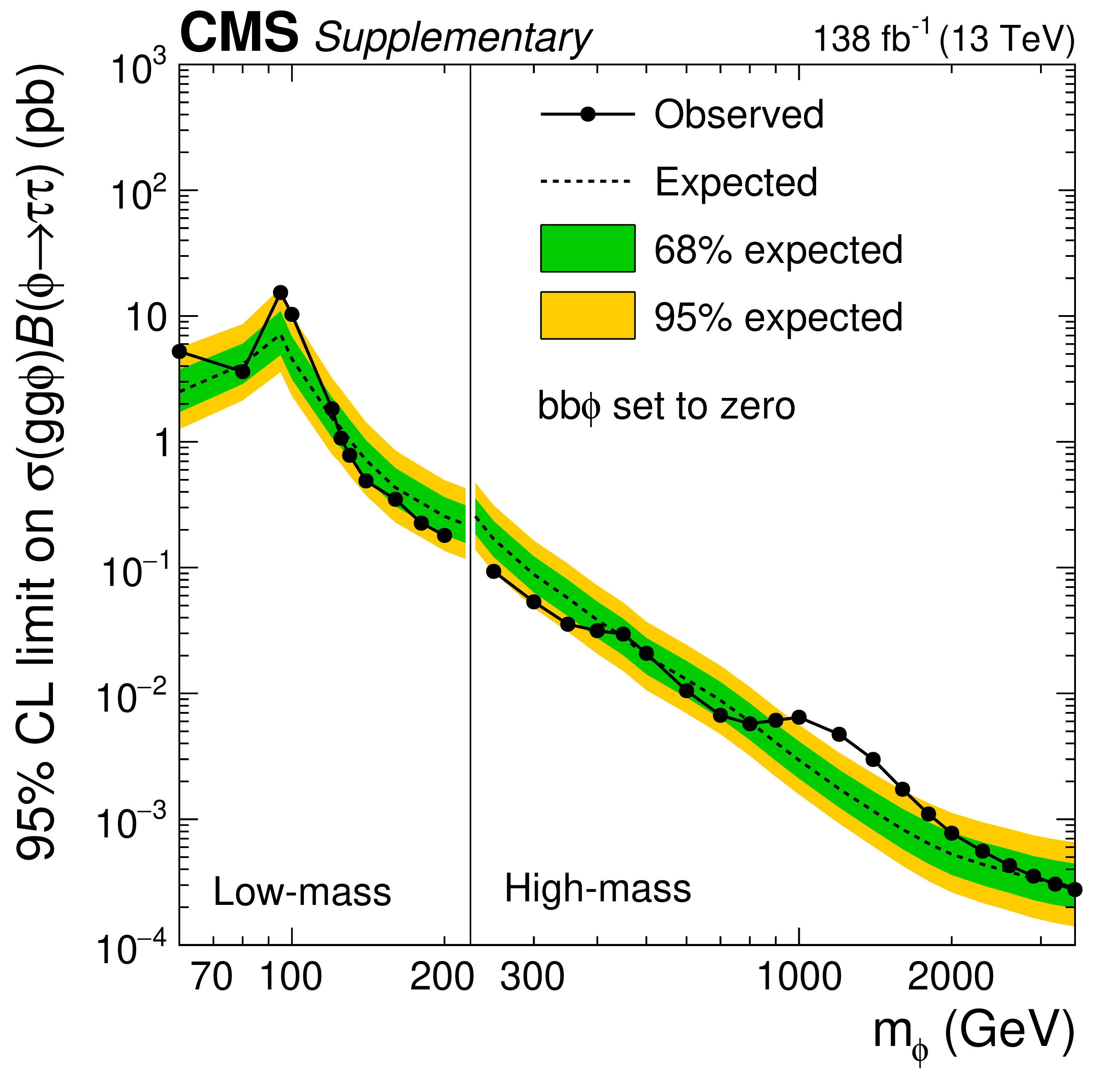
Additional Figure 37:
Expected and observed 95% CL upper limits on the product of the cross sections and branching fraction for the decay into $ \tau $ leptons for $ \mathrm{g} \mathrm{g} \phi$ production in a mass range of 60 $ < m_{\phi}< $ 3500 GeV. The expected median of the exclusion limit in the absence of signal is shown by the dashed line. The dark green and bright yellow bands indicate the central 68% and 95% intervals for the expected exclusion limits. The black dots correspond to the observed limits. For this figure the $ \mathrm{b} \mathrm{b} \phi$ production rate has been fixed to zero. |
png pdf |
Additional Figure 38:
Expected and observed 95% CL upper limits on the product of the cross sections and branching fraction for the decay into $ \tau $ leptons for $ \mathrm{b} \mathrm{b} \phi$ production in a mass range of 60 $ < m_{\phi} < $ 3500 GeV. The expected median of the exclusion limit in the absence of signal is shown by the dashed line. The dark green and bright yellow bands indicate the central 68% and 95% intervals for the expected exclusion limits. The black dots correspond to the observed limits. For this figure the $ \mathrm{g} \mathrm{g} \phi$ production rate has been fixed to zero. |
png pdf |
Additional Figure 39:
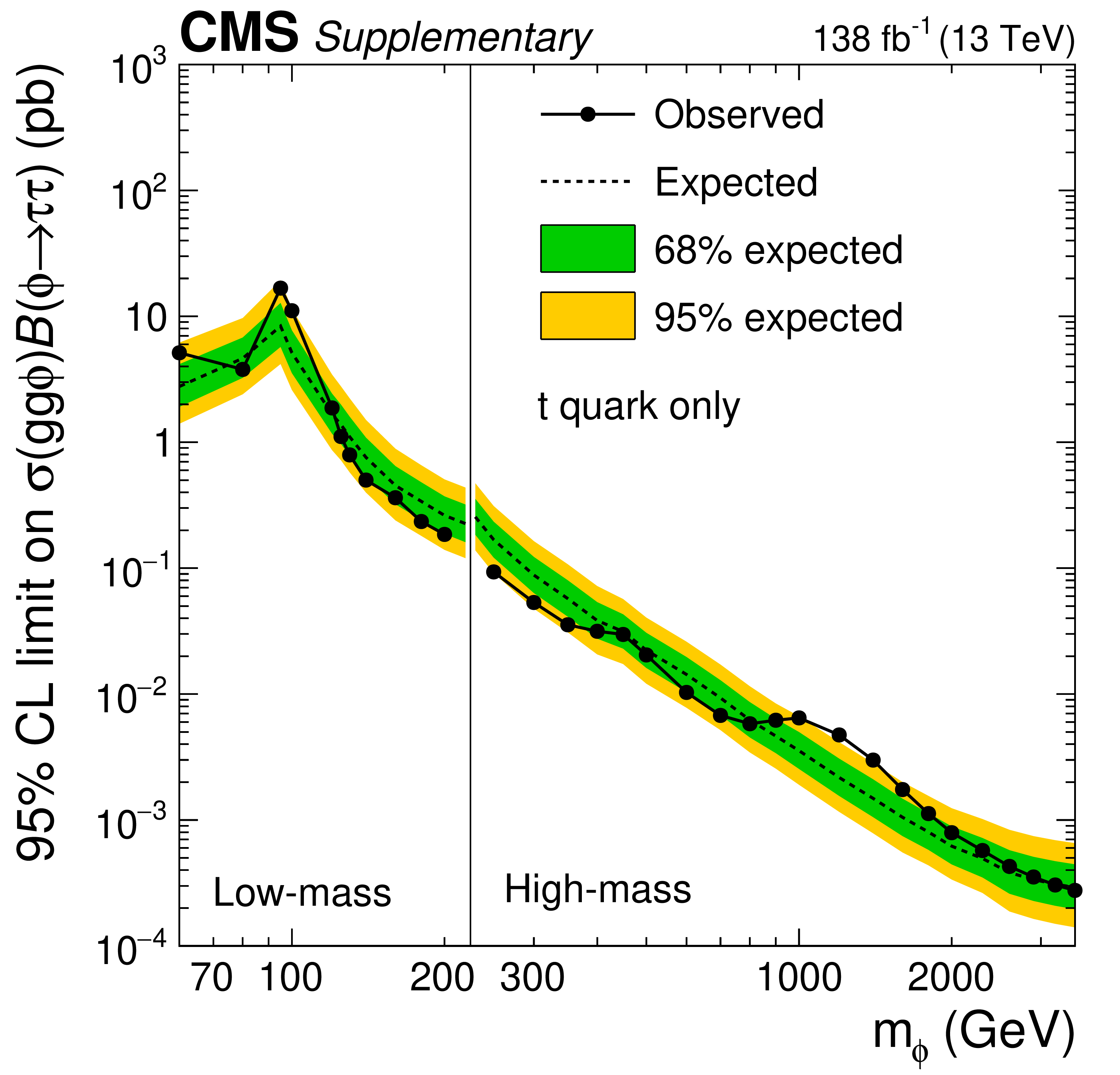
Expected and observed 95% CL upper limits on the product of the cross sections and branching fraction for the decay into $ \tau $ leptons for $ \mathrm{g} \mathrm{g} \phi$ production in a mass range of 60 $ < m_{\phi} < $ 3500 GeV. The expected median of the exclusion limit in the absence of signal is shown by the dashed line. The dark green and bright yellow bands indicate the central 68% and 95% intervals for the expected exclusion limits. The black dots correspond to the observed limits. For this figure the $ \mathrm{b} \mathrm{b} \phi$ production rate has been profiled and only t quarks are considered in the $ \mathrm{g} \mathrm{g} \phi$ loop. |
png pdf |
Additional Figure 40:
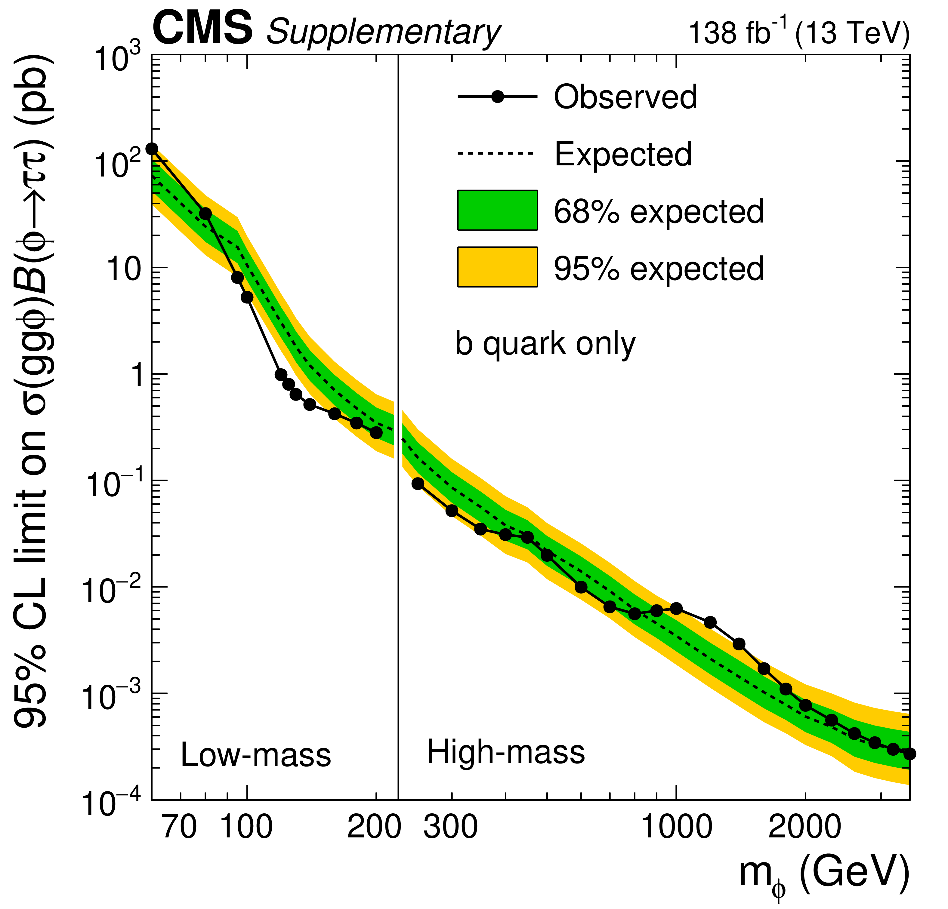
Expected and observed 95% CL upper limits on the product of the cross sections and branching fraction for the decay into $ \tau $ leptons for $ \mathrm{g} \mathrm{g} \phi$ production in a mass range of 60 $ < m_{\phi} < $ 3500 GeV. The expected median of the exclusion limit in the absence of signal is shown by the dashed line. The dark green and bright yellow bands indicate the central 68% and 95% intervals for the expected exclusion limits. The black dots correspond to the observed limits. For this figure the $ \mathrm{b} \mathrm{b} \phi$ production rate has been profiled and only b quarks are considered in the $ \mathrm{g} \mathrm{g} \phi$ loop. |
png pdf |
Additional Figure 41:
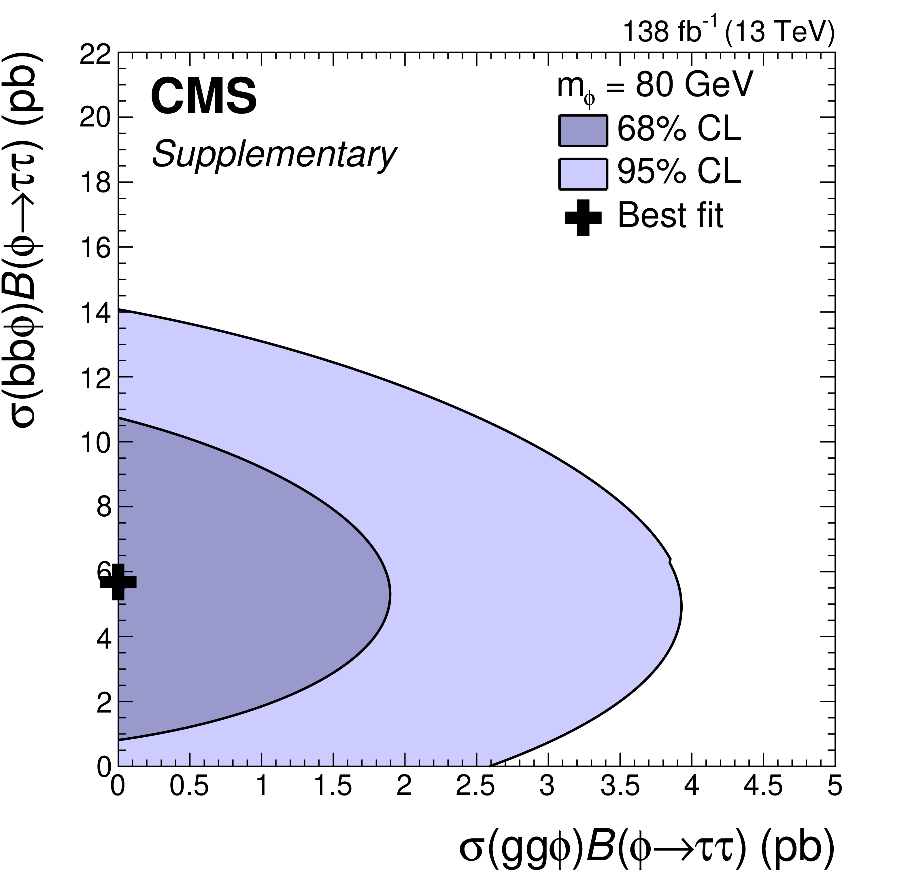
Maximum likelihood estimate, and 68% and 95% CL contours obtained from scans of the signal likelihood for the model-independent $\phi$ search. The scans are shown for $m_{\phi}= $ 80 GeV. The SM expectation is $(0, 0)$. |

png pdf |
Additional Figure 42:
Maximum likelihood estimate, and 68% and 95% CL contours obtained from scans of the signal likelihood for the model-independent $\phi$ search. The scans are shown for $m_{\phi}= $ 95 GeV. The SM expectation is $(0, 0)$. |
png pdf |
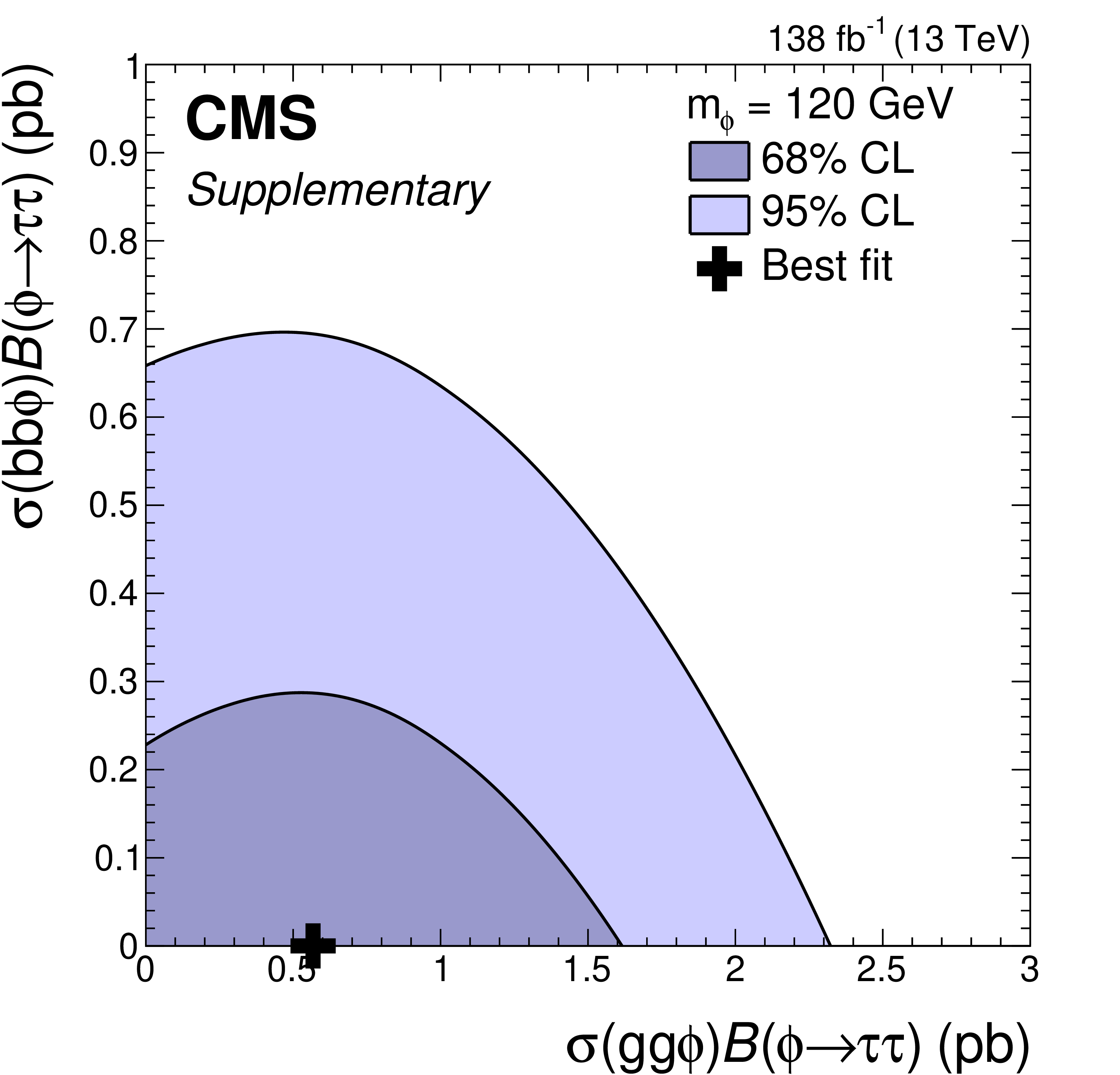
Additional Figure 43:
Maximum likelihood estimate, and 68% and 95% CL contours obtained from scans of the signal likelihood for the model-independent $\phi$ search. The scans are shown for $m_{\phi}= $ 120 GeV. The SM expectation is $(0, 0)$. |
png pdf |
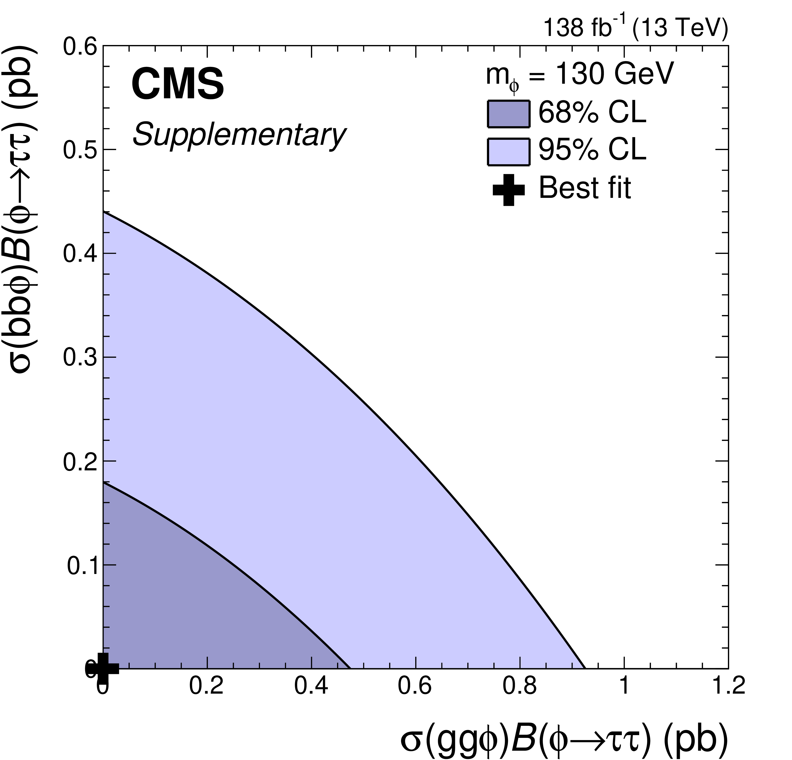
Additional Figure 44:
Maximum likelihood estimate, and 68% and 95% CL contours obtained from scans of the signal likelihood for the model-independent $\phi$ search. The scans are shown for $m_{\phi}= $ 130 GeV. The SM expectation is $(0, 0)$. |
png pdf |
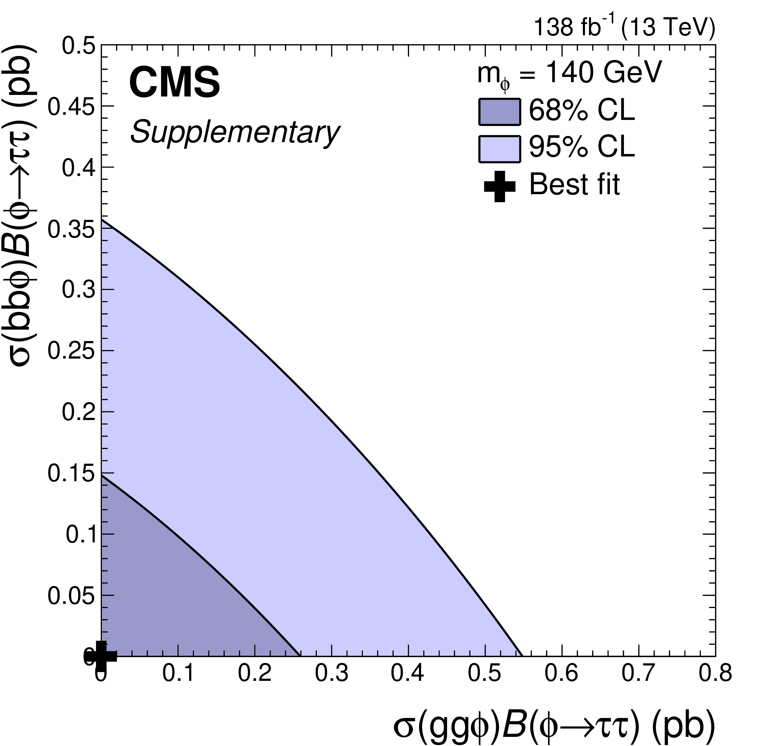
Additional Figure 45:
Maximum likelihood estimate, and 68% and 95% CL contours obtained from scans of the signal likelihood for the model-independent $\phi$ search. The scans are shown for $m_{\phi}= $ 140 GeV. The SM expectation is $(0, 0)$. |
png pdf |
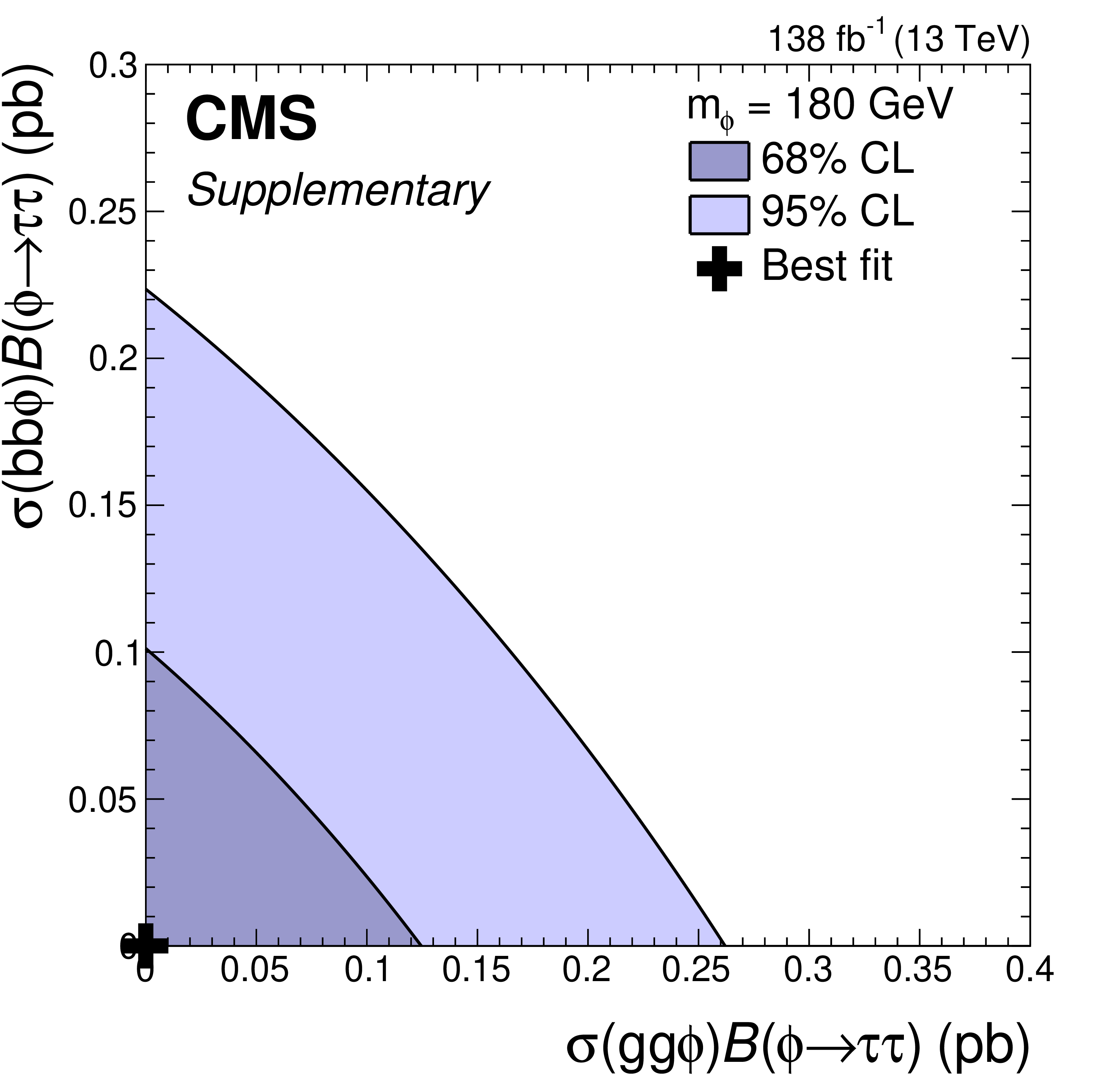
Additional Figure 46:
Maximum likelihood estimate, and 68% and 95% CL contours obtained from scans of the signal likelihood for the model-independent $\phi$ search. The scans are shown for $m_{\phi}= $ 180 GeV. The SM expectation is $(0, 0)$. |
png pdf |
Additional Figure 47:
Maximum likelihood estimate, and 68% and 95% CL contours obtained from scans of the signal likelihood for the model-independent $\phi$ search. The scans are shown for $m_{\phi}= $ 200 GeV. The SM expectation is $(0, 0)$. |

png pdf |
Additional Figure 48:
Maximum likelihood estimate, and 68% and 95% CL contours obtained from scans of the signal likelihood for the model-independent $\phi$ search. The scans are shown for $m_{\phi}= $ 300 GeV. The SM expectation is $(0, 0)$. |

png pdf |
Additional Figure 49:
Maximum likelihood estimate, and 68% and 95% CL contours obtained from scans of the signal likelihood for the model-independent $\phi$ search. The scans are shown for $m_{\phi}= $ 350 GeV. The SM expectation is $(0, 0)$. |

png pdf |
Additional Figure 50:
Maximum likelihood estimate, and 68% and 95% CL contours obtained from scans of the signal likelihood for the model-independent $\phi$ search. The scans are shown for $m_{\phi}= $ 400 GeV. The SM expectation is $(0, 0)$. |
png pdf |
Additional Figure 51:
Maximum likelihood estimate, and 68% and 95% CL contours obtained from scans of the signal likelihood for the model-independent $\phi$ search. The scans are shown for $m_{\phi}= $ 450 GeV. The SM expectation is $(0, 0)$. |
png pdf |
Additional Figure 52:
Maximum likelihood estimate, and 68% and 95% CL contours obtained from scans of the signal likelihood for the model-independent $\phi$ search. The scans are shown for $m_{\phi}= $ 600 GeV. The SM expectation is $(0, 0)$. |
png pdf |
Additional Figure 53:
Maximum likelihood estimate, and 68% and 95% CL contours obtained from scans of the signal likelihood for the model-independent $\phi$ search. The scans are shown for $m_{\phi}= $ 700 GeV. The SM expectation is $(0, 0)$. |

png pdf |
Additional Figure 54:
Maximum likelihood estimate, and 68% and 95% CL contours obtained from scans of the signal likelihood for the model-independent $\phi$ search. The scans are shown for $m_{\phi}= $ 800 GeV. The SM expectation is $(0, 0)$. |
png pdf |
Additional Figure 55:
Maximum likelihood estimate, and 68% and 95% CL contours obtained from scans of the signal likelihood for the model-independent $\phi$ search. The scans are shown for $m_{\phi}= $ 900 GeV. The SM expectation is $(0, 0)$. |
png pdf |
Additional Figure 56:
Maximum likelihood estimate, and 68% and 95% CL contours obtained from scans of the signal likelihood for the model-independent $\phi$ search. The scans are shown for $m_{\phi}= $ 1400 GeV. The SM expectation is $(0, 0)$. |
png pdf |
Additional Figure 57:
Maximum likelihood estimate, and 68% and 95% CL contours obtained from scans of the signal likelihood for the model-independent $\phi$ search. The scans are shown for $m_{\phi}= $ 1600 GeV. The SM expectation is $(0, 0)$. |
png pdf |
Additional Figure 58:
Maximum likelihood estimate, and 68% and 95% CL contours obtained from scans of the signal likelihood for the model-independent $\phi$ search. The scans are shown for $m_{\phi}= $ 1800 GeV. The SM expectation is $(0, 0)$. |
png pdf |
Additional Figure 59:
Maximum likelihood estimate, and 68% and 95% CL contours obtained from scans of the signal likelihood for the model-independent $\phi$ search. The scans are shown for $m_{\phi}= $ 2000 GeV. The SM expectation is $(0, 0)$. |

png pdf |
Additional Figure 60:
Maximum likelihood estimate, and 68% and 95% CL contours obtained from scans of the signal likelihood for the model-independent $\phi$ search. The scans are shown for $m_{\phi}= $ 2300 GeV. The SM expectation is $(0, 0)$. |
png pdf |
Additional Figure 61:
Maximum likelihood estimate, and 68% and 95% CL contours obtained from scans of the signal likelihood for the model-independent $\phi$ search. The scans are shown for $m_{\phi}= $ 2600 GeV. The SM expectation is $(0, 0)$. |

png pdf |
Additional Figure 62:
Maximum likelihood estimate, and 68% and 95% CL contours obtained from scans of the signal likelihood for the model-independent $\phi$ search. The scans are shown for $m_{\phi}= $ 2900 GeV. The SM expectation is $(0, 0)$. |
png pdf |
Additional Figure 63:
Maximum likelihood estimate, and 68% and 95% CL contours obtained from scans of the signal likelihood for the model-independent $\phi$ search. The scans are shown for $m_{\phi}= $ 3200 GeV. The SM expectation is $(0, 0)$. |
png pdf |
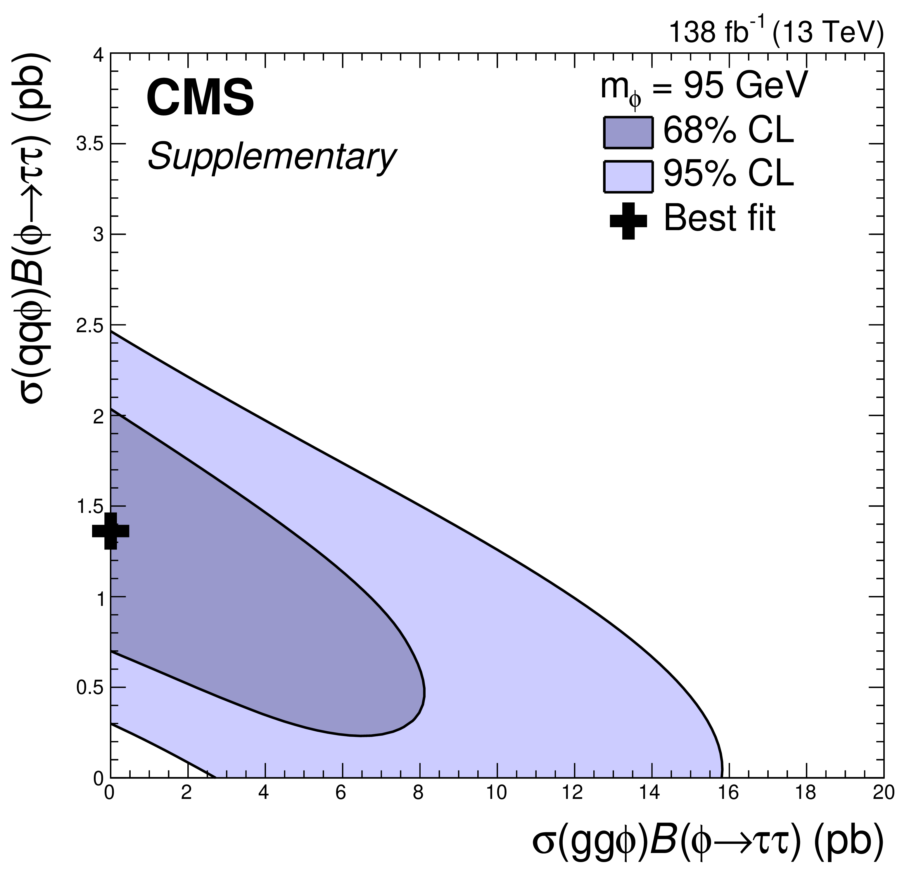
Additional Figure 64:
Maximum likelihood estimate, and 68% and 95% CL contours obtained from scans of the signal likelihood for a $\phi$ resonance with $m_{\phi}= $ 95 GeV, produced via $ \mathrm{g} \mathrm{g} \phi$ or vector boson fusion ($ \mathrm{q} \mathrm{q} \phi$). For this figure the $ \mathrm{b} \mathrm{b} \phi$ production rate has been profiled. |
png pdf |
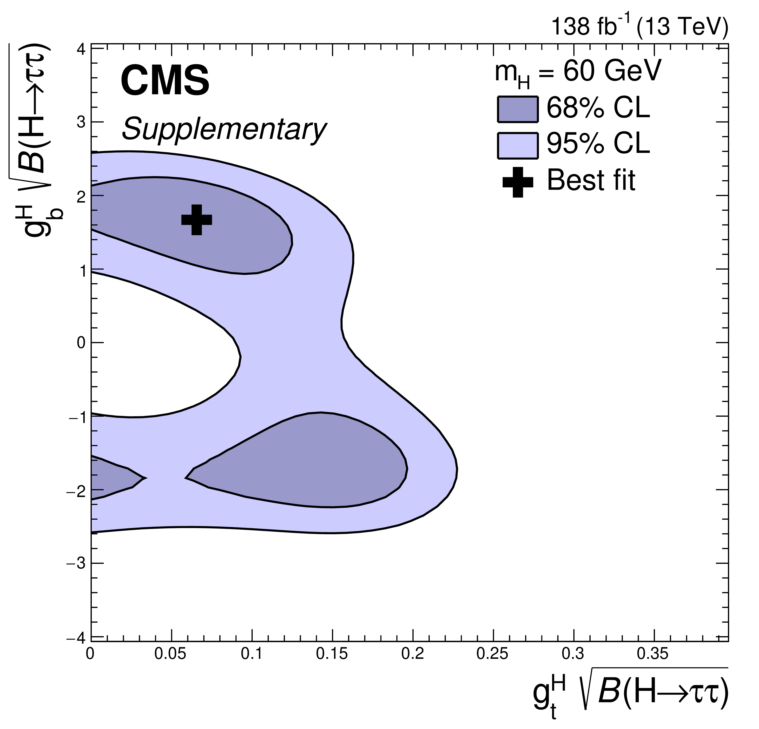
Additional Figure 65:
Maximum likelihood estimate, and 68% and 95% CL contours obtained from scans of the signal-plus-background likelihood for a scalar resonance $ \mathrm{H} $ with $m_{\mathrm{H}}= $ 60 GeV, produced via $ \mathrm{g} \mathrm{g} \mathrm{H}$ or $ \mathrm{b} \mathrm{b} \mathrm{H}$. For this scan, we assume that both processes are only influenced by the Yukawa couplings to t and b quarks and scale the predicted cross sections depending on these couplings. The estimates are shown for the product of the reduced Yukawa couplings $\mathrm{g}_{ \mathrm{t} ,\, \mathrm{b} }^{\mathrm{H}}$ and $\sqrt{B(\mathrm{H}\to \tau \tau )}$, where the former is defined as the ratio of the Yukawa coupling of $ \mathrm{H} $ over the Yukawa coupling expected for a SM-like Higgs boson of the same mass. An ambiguity on the relative sign of the two couplings can be resolved by the contribution of $ \mathrm{t} \mathrm{b} $-interference terms to the cross section predictions. By convention $\mathrm{g}_{ \mathrm{t} }^{\mathrm{H}}$ has been chosen positive. |
png pdf |
Additional Figure 66:
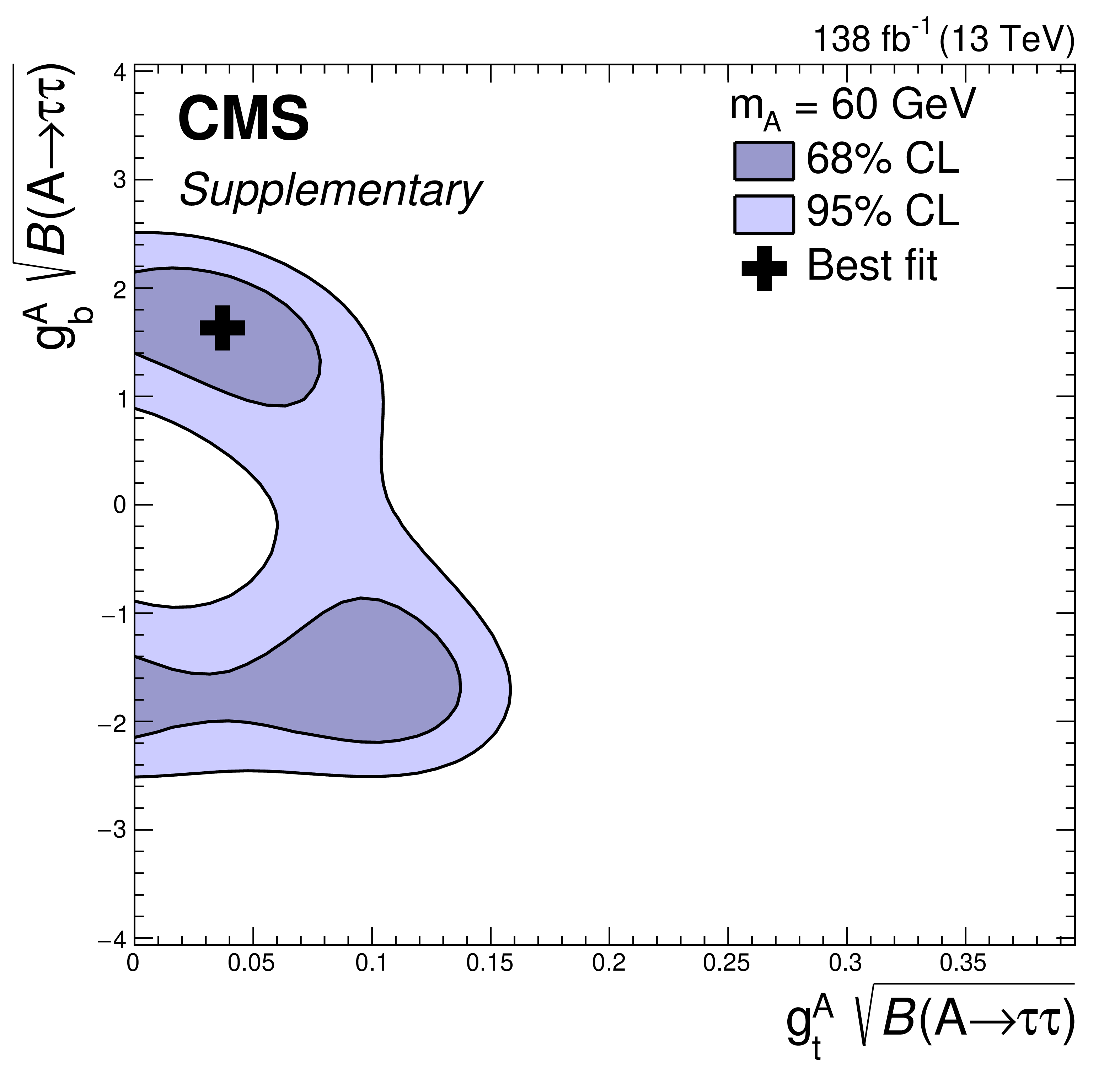
Maximum likelihood estimate, and 68% and 95% CL contours obtained from scans of the signal-plus-background likelihood for a pseudoscalar resonance $\mathrm{A}$ with $m_{\mathrm{A}}= $ 60 GeV, produced via $ \mathrm{g} \mathrm{g} \mathrm{A}$ or $ \mathrm{b} \mathrm{b} \mathrm{A}$. For this scan, we assume that both processes are only influenced by the Yukawa couplings to t and b quarks and scale the predicted cross sections depending on these couplings. The estimates are shown for the product of the reduced Yukawa couplings $\mathrm{g}_{ \mathrm{t} ,\, \mathrm{b} }^{\mathrm{A}}$ and $\sqrt{B(\mathrm{A}\to \tau \tau )}$, where the former is defined as the ratio of the Yukawa coupling of $\mathrm{A}$ over the Yukawa coupling expected for a SM-like Higgs boson of the same mass. An ambiguity on the relative sign of the two couplings can be resolved by the contribution of $ \mathrm{t} \mathrm{b} $-interference terms to the cross section predictions. By convention $\mathrm{g}_{ \mathrm{t} }^{\mathrm{A}}$ has been chosen positive. |
png pdf |
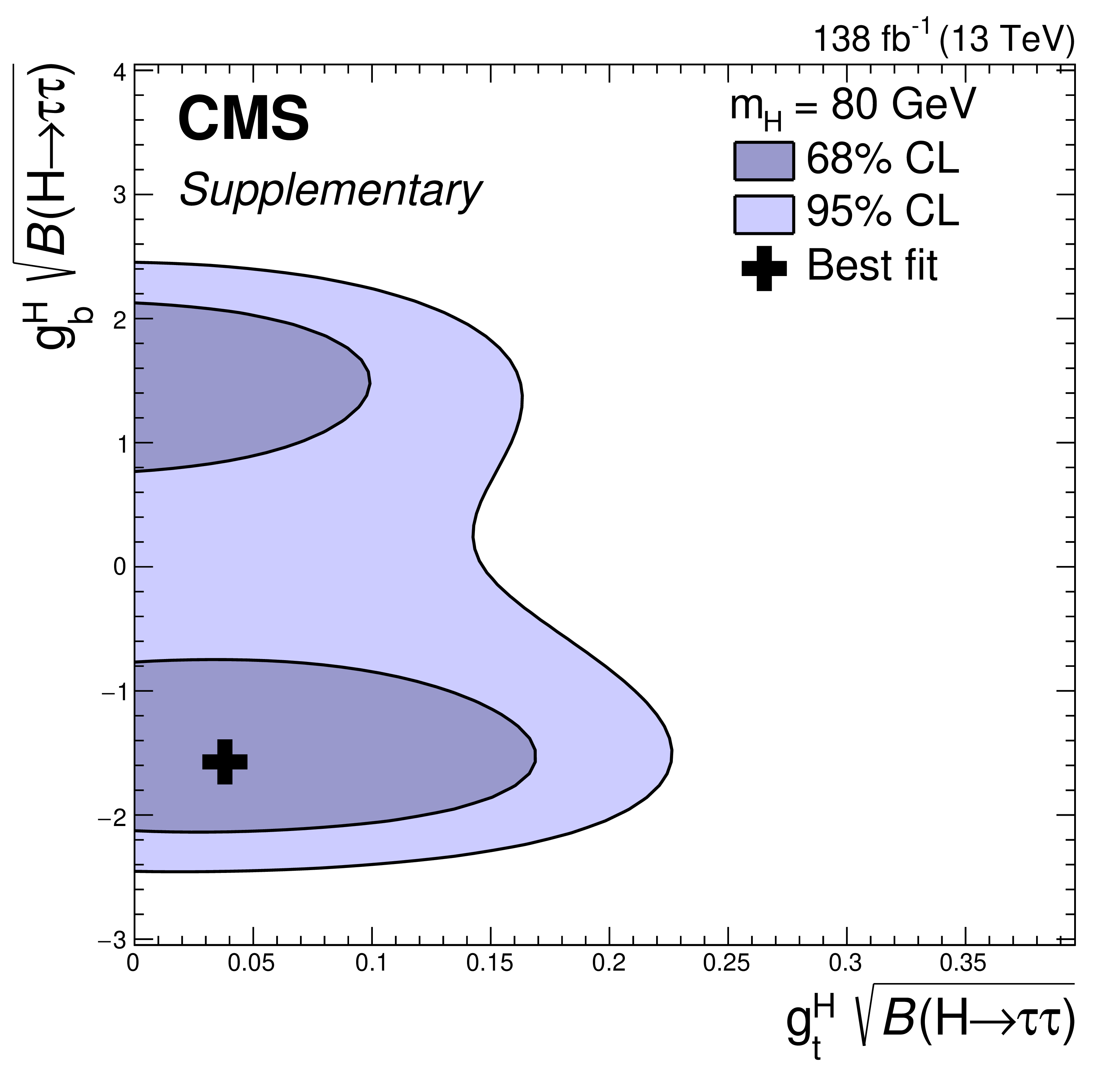
Additional Figure 67:
Maximum likelihood estimate, and 68% and 95% CL contours obtained from scans of the signal-plus-background likelihood for a scalar resonance ($ \mathrm{H} $) with $m_{\mathrm{H}}= $ 80 GeV, produced via $ \mathrm{g} \mathrm{g} \mathrm{H}$ or $ \mathrm{b} \mathrm{b} \mathrm{H}$. For this scan, we assume that both processes are only influenced by the Yukawa couplings to t and b quarks and scale the predicted cross sections depending on these couplings. The estimates are shown for the product of the reduced Yukawa couplings $\mathrm{g}_{ \mathrm{t} ,\, \mathrm{b} }^{\mathrm{H}}$ and $\sqrt{B(\mathrm{H}\to \tau \tau )}$, where the former is defined as the ratio of the Yukawa coupling of $ \mathrm{H} $ over the Yukawa coupling expected for a SM-like Higgs boson of the same mass. An ambiguity on the relative sign of the two couplings can be resolved by the contribution of $ \mathrm{t} \mathrm{b} $-interference terms to the cross section predictions. By convention $\mathrm{g}_{ \mathrm{t} }^{\mathrm{H}}$ has been chosen positive. |
png pdf |
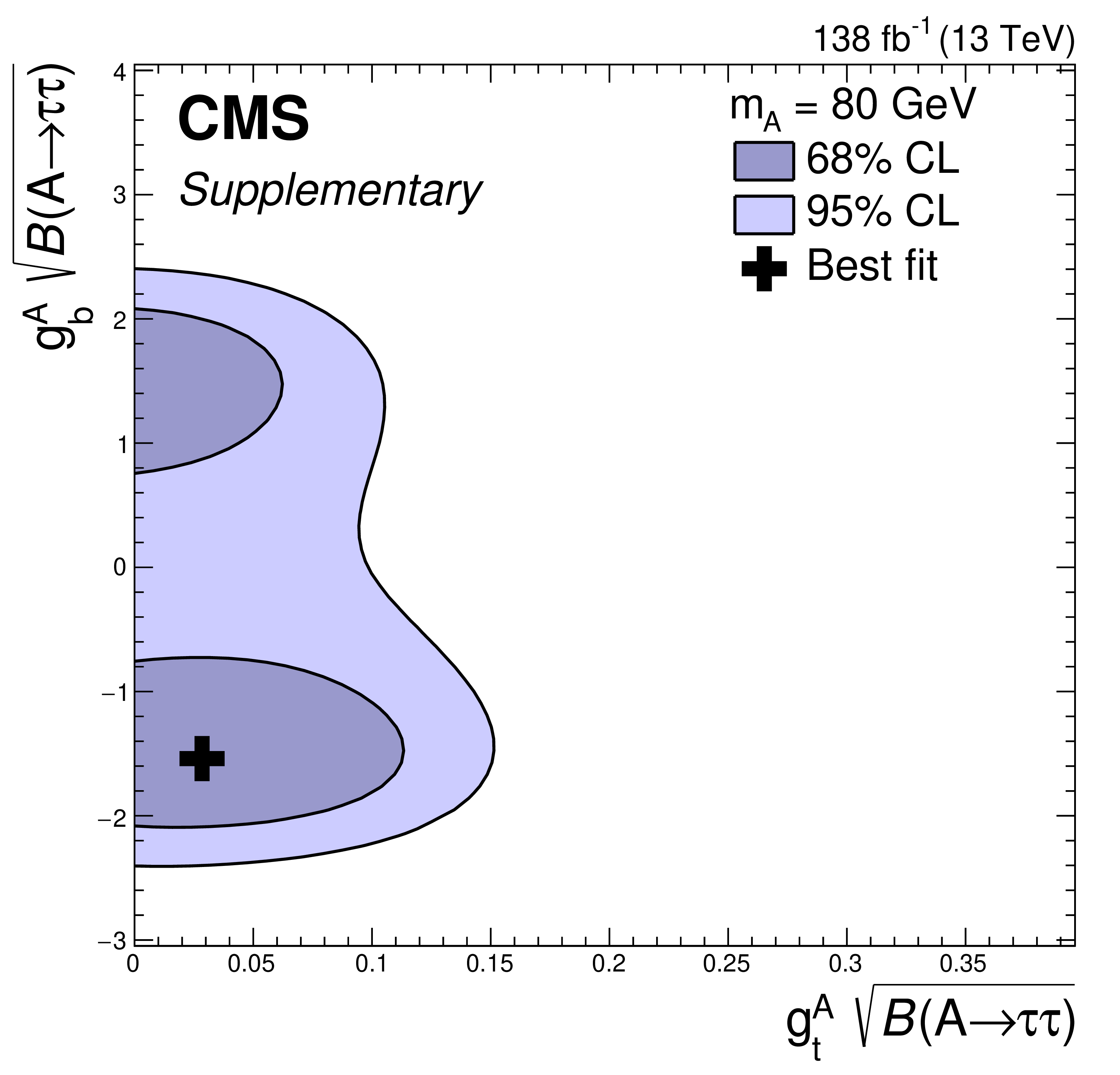
Additional Figure 68:
Maximum likelihood estimate, and 68% and 95% CL contours obtained from scans of the signal-plus-background likelihood for a pseudoscalar resonance ($\mathrm{A}$) with $m_{\mathrm{A}}= $ 80 GeV, produced via $ \mathrm{g} \mathrm{g} \mathrm{A}$ or $ \mathrm{b} \mathrm{b} \mathrm{A}$. For this scan, we assume that both processes are only influenced by the Yukawa couplings to t and b quarks and scale the predicted cross sections depending on these couplings. The estimates are shown for the product of the reduced Yukawa couplings $\mathrm{g}_{ \mathrm{t} ,\, \mathrm{b} }^{\mathrm{A}}$ and $\sqrt{B(\mathrm{A}\to \tau \tau )}$, where the former is defined as the ratio of the Yukawa coupling of $\mathrm{A}$ over the Yukawa coupling expected for a SM-like Higgs boson of the same mass. An ambiguity on the relative sign of the two couplings can be resolved by the contribution of $ \mathrm{t} \mathrm{b} $-interference terms to the cross section predictions. By convention $\mathrm{g}_{ \mathrm{t} }^{\mathrm{A}}$ has been chosen positive. |
png pdf |
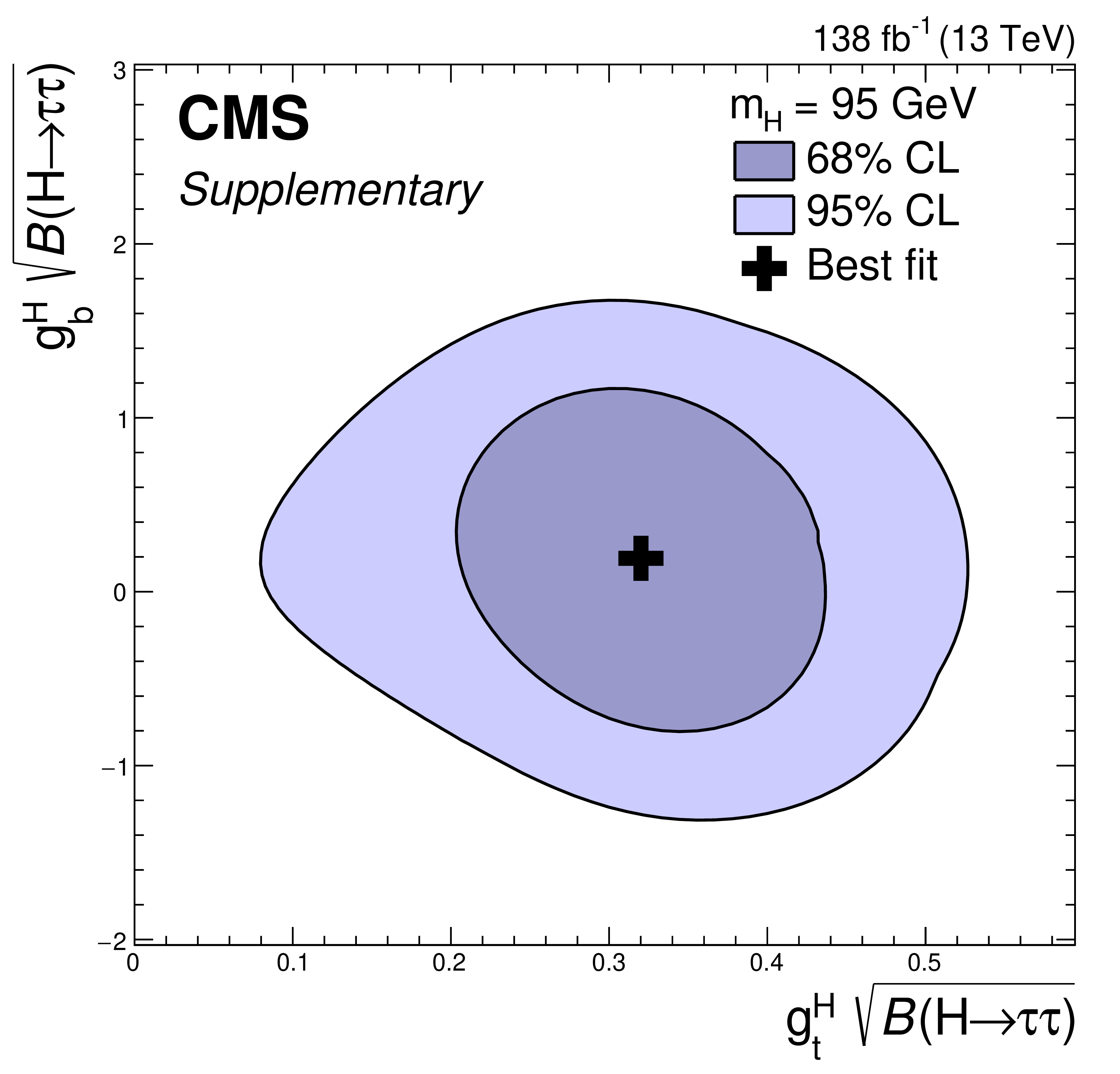
Additional Figure 69:
Maximum likelihood estimate, and 68% and 95% CL contours obtained from scans of the signal-plus-background likelihood for a scalar resonance ($ \mathrm{H} $) with $m_{\mathrm{H}}= $ 95 GeV, produced via $ \mathrm{g} \mathrm{g} \mathrm{H}$ or $ \mathrm{b} \mathrm{b} \mathrm{H}$. For this scan, we assume that both processes are only influenced by the Yukawa couplings to t and b quarks and scale the predicted cross sections depending on these couplings. The estimates are shown for the product of the reduced Yukawa couplings $\mathrm{g}_{ \mathrm{t} ,\, \mathrm{b} }^{\mathrm{H}}$ and $\sqrt{B(\mathrm{H}\to \tau \tau )}$, where the former is defined as the ratio of the Yukawa coupling of $ \mathrm{H} $ over the Yukawa coupling expected for a SM-like Higgs boson of the same mass. An ambiguity on the relative sign of the two couplings can be resolved by the contribution of $ \mathrm{t} \mathrm{b} $-interference terms to the cross section predictions. By convention $\mathrm{g}_{ \mathrm{t} }^{\mathrm{H}}$ has been chosen positive. |
png pdf |
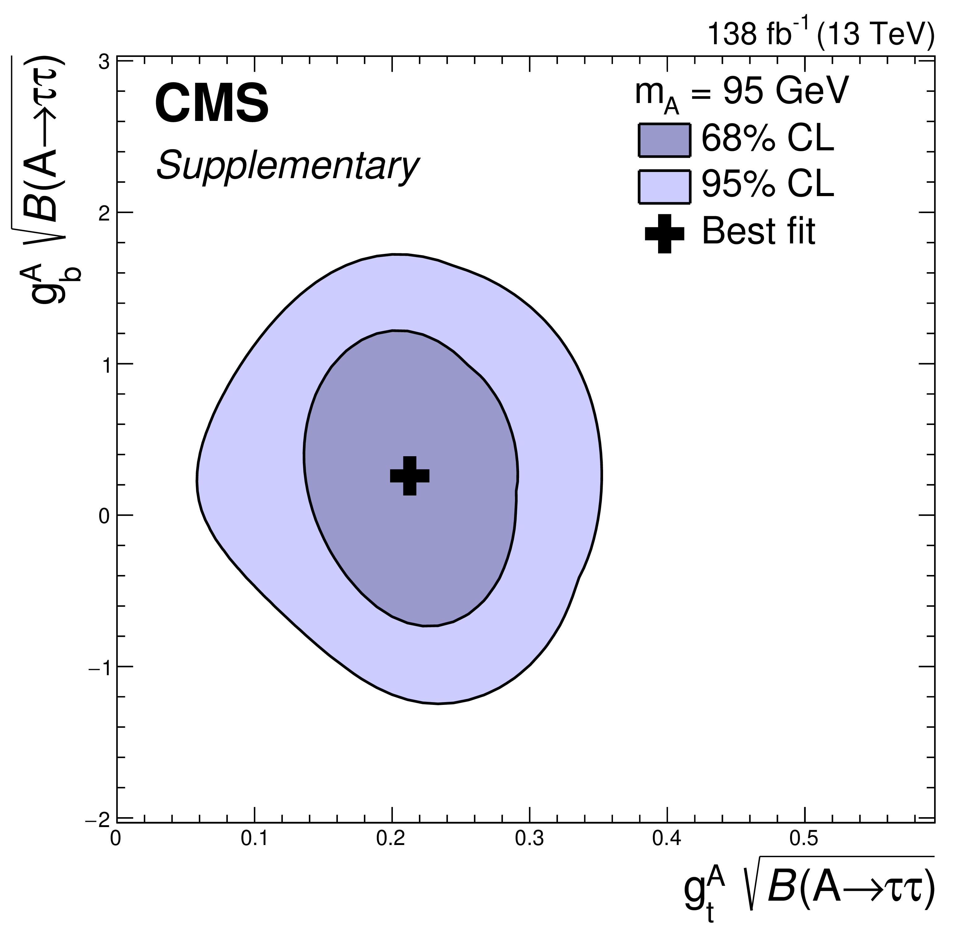
Additional Figure 70:
Maximum likelihood estimate, and 68% and 95% CL contours obtained from scans of the signal-plus-background likelihood for a pseudoscalar resonance ($\mathrm{A}$) with $m_{\mathrm{A}}= $ 95 GeV, produced via $ \mathrm{g} \mathrm{g} \mathrm{A}$ or $ \mathrm{b} \mathrm{b} \mathrm{A}$. For this scan, we assume that both processes are only influenced by the Yukawa couplings to t and b quarks and scale the predicted cross sections depending on these couplings. The estimates are shown for the product of the reduced Yukawa couplings $\mathrm{g}_{ \mathrm{t} ,\, \mathrm{b} }^{\mathrm{A}}$ and $\sqrt{B(\mathrm{A}\to \tau \tau )}$, where the former is defined as the ratio of the Yukawa coupling of $\mathrm{A}$ over the Yukawa coupling expected for a SM-like Higgs boson of the same mass. An ambiguity on the relative sign of the two couplings can be resolved by the contribution of $ \mathrm{t} \mathrm{b} $-interference terms to the cross section predictions. By convention $\mathrm{g}_{ \mathrm{t} }^{\mathrm{A}}$ has been chosen positive. |
png pdf |
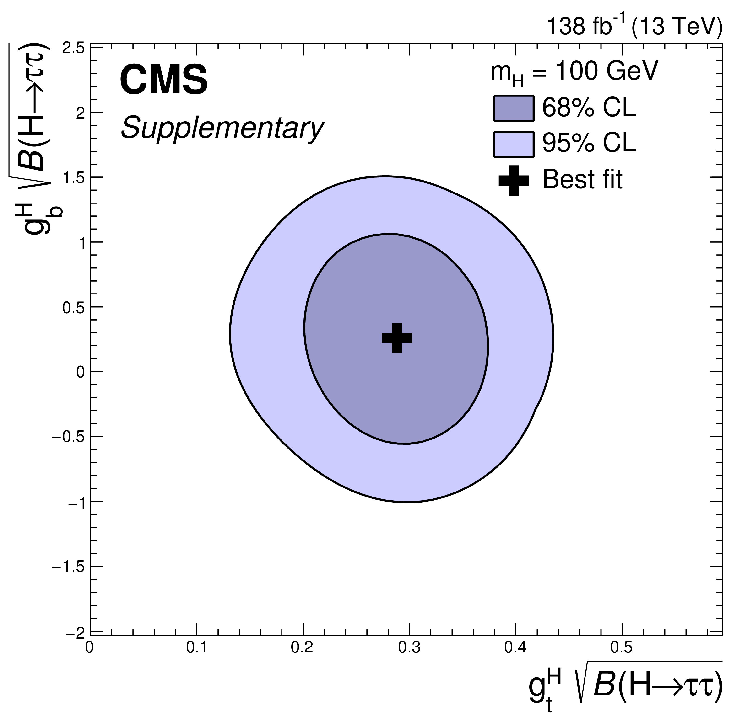
Additional Figure 71:
Maximum likelihood estimate, and 68% and 95% CL contours obtained from scans of the signal-plus-background likelihood for a scalar resonance ($ \mathrm{H} $) with $m_{\mathrm{H}}= $ 100 GeV, produced via $ \mathrm{g} \mathrm{g} \mathrm{H}$ or $ \mathrm{b} \mathrm{b} \mathrm{H}$. For this scan, we assume that both processes are only influenced by the Yukawa couplings to t and b quarks and scale the predicted cross sections depending on these couplings. The estimates are shown for the product of the reduced Yukawa couplings $\mathrm{g}_{ \mathrm{t} ,\, \mathrm{b} }^{\mathrm{H}}$ and $\sqrt{B(\mathrm{H}\to \tau \tau )}$, where the former is defined as the ratio of the Yukawa coupling of $ \mathrm{H} $ over the Yukawa coupling expected for a SM-like Higgs boson of the same mass. An ambiguity on the relative sign of the two couplings can be resolved by the contribution of $ \mathrm{t} \mathrm{b} $-interference terms to the cross section predictions. By convention $\mathrm{g}_{ \mathrm{t} }^{\mathrm{H}}$ has been chosen positive. |
png pdf |
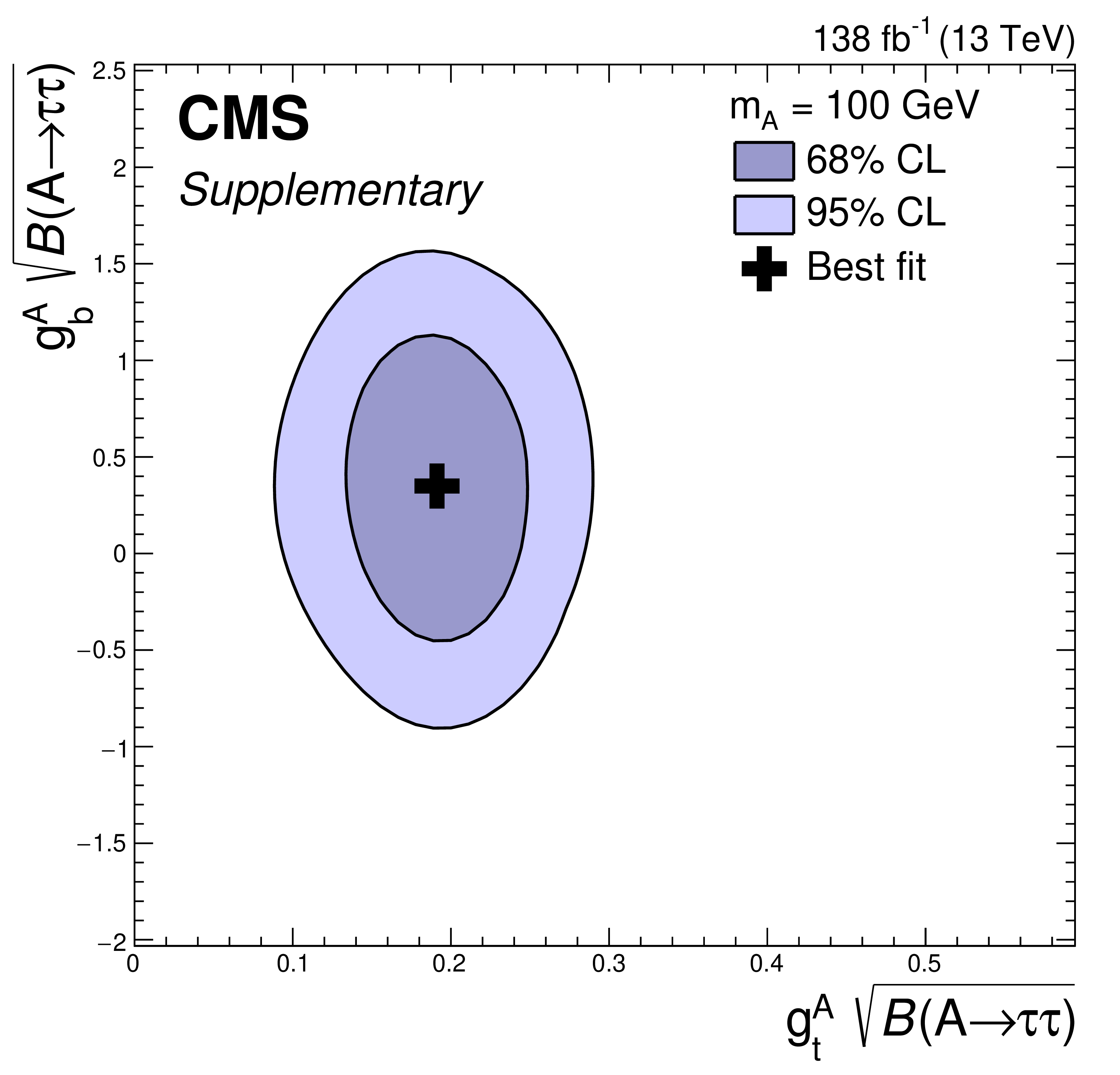
Additional Figure 72:
Maximum likelihood estimate, and 68% and 95% CL contours obtained from scans of the signal-plus-background likelihood for a pseudoscalar resonance ($\mathrm{A}$) with $m_{\mathrm{A}}= $ 100 GeV, produced via $ \mathrm{g} \mathrm{g} \mathrm{A}$ or $ \mathrm{b} \mathrm{b} \mathrm{A}$. For this scan, we assume that both processes are only influenced by the Yukawa couplings to t and b quarks and scale the predicted cross sections depending on these couplings. The estimates are shown for the product of the reduced Yukawa couplings $\mathrm{g}_{ \mathrm{t} ,\, \mathrm{b} }^{\mathrm{A}}$ and $\sqrt{B(\mathrm{A}\to \tau \tau )}$, where the former is defined as the ratio of the Yukawa coupling of $\mathrm{A}$ over the Yukawa coupling expected for a SM-like Higgs boson of the same mass. An ambiguity on the relative sign of the two couplings can be resolved by the contribution of $ \mathrm{t} \mathrm{b} $-interference terms to the cross section predictions. By convention $\mathrm{g}_{ \mathrm{t} }^{\mathrm{A}}$ has been chosen positive. |
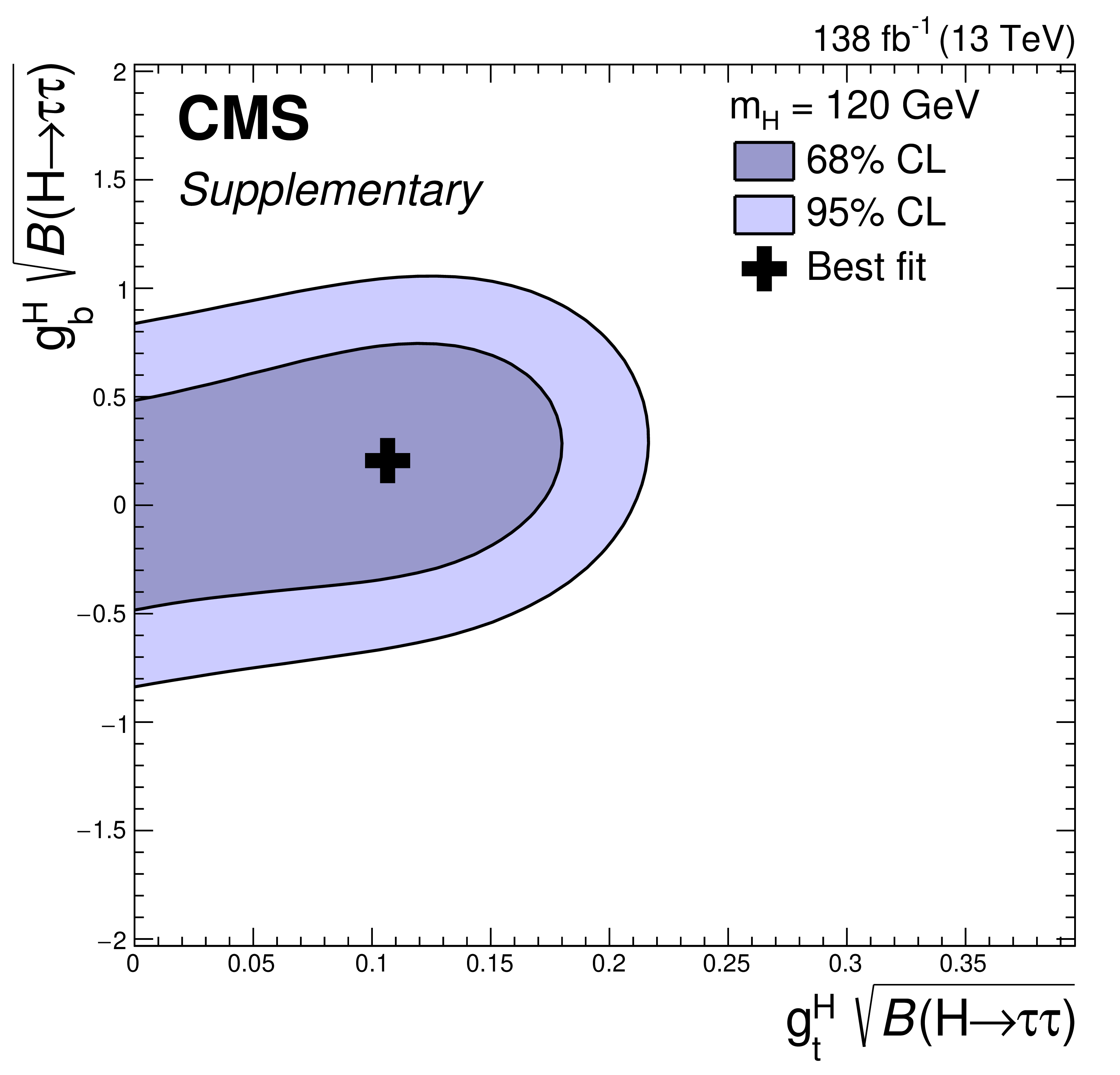
png pdf |
Additional Figure 73:
Maximum likelihood estimate, and 68% and 95% CL contours obtained from scans of the signal-plus-background likelihood for a scalar resonance ($ \mathrm{H} $) with $m_{\mathrm{H}}= $ 120 GeV, produced via $ \mathrm{g} \mathrm{g} \mathrm{H}$ or $ \mathrm{b} \mathrm{b} \mathrm{H}$. For this scan, we assume that both processes are only influenced by the Yukawa couplings to t and b quarks and scale the predicted cross sections depending on these couplings. The estimates are shown for the product of the reduced Yukawa couplings $\mathrm{g}_{ \mathrm{t} ,\, \mathrm{b} }^{\mathrm{H}}$ and $\sqrt{B(\mathrm{H}\to \tau \tau )}$, where the former is defined as the ratio of the Yukawa coupling of $ \mathrm{H} $ over the Yukawa coupling expected for a SM-like Higgs boson of the same mass. An ambiguity on the relative sign of the two couplings can be resolved by the contribution of $ \mathrm{t} \mathrm{b} $-interference terms to the cross section predictions. By convention $\mathrm{g}_{ \mathrm{t} }^{\mathrm{H}}$ has been chosen positive. |

png pdf |
Additional Figure 74:
Maximum likelihood estimate, and 68% and 95% CL contours obtained from scans of the signal-plus-background likelihood for a pseudoscalar resonance ($\mathrm{A}$) with $m_{\mathrm{A}}= $ 120 GeV, produced via $ \mathrm{g} \mathrm{g} \mathrm{A}$ or $ \mathrm{b} \mathrm{b} \mathrm{A}$. For this scan, we assume that both processes are only influenced by the Yukawa couplings to t and b quarks and scale the predicted cross sections depending on these couplings. The estimates are shown for the product of the reduced Yukawa couplings $\mathrm{g}_{ \mathrm{t} ,\, \mathrm{b} }^{\mathrm{A}}$ and $\sqrt{B(\mathrm{A}\to \tau \tau )}$, where the former is defined as the ratio of the Yukawa coupling of $\mathrm{A}$ over the Yukawa coupling expected for a SM-like Higgs boson of the same mass. An ambiguity on the relative sign of the two couplings can be resolved by the contribution of $ \mathrm{t} \mathrm{b} $-interference terms to the cross section predictions. By convention $\mathrm{g}_{ \mathrm{t} }^{\mathrm{A}}$ has been chosen positive. |
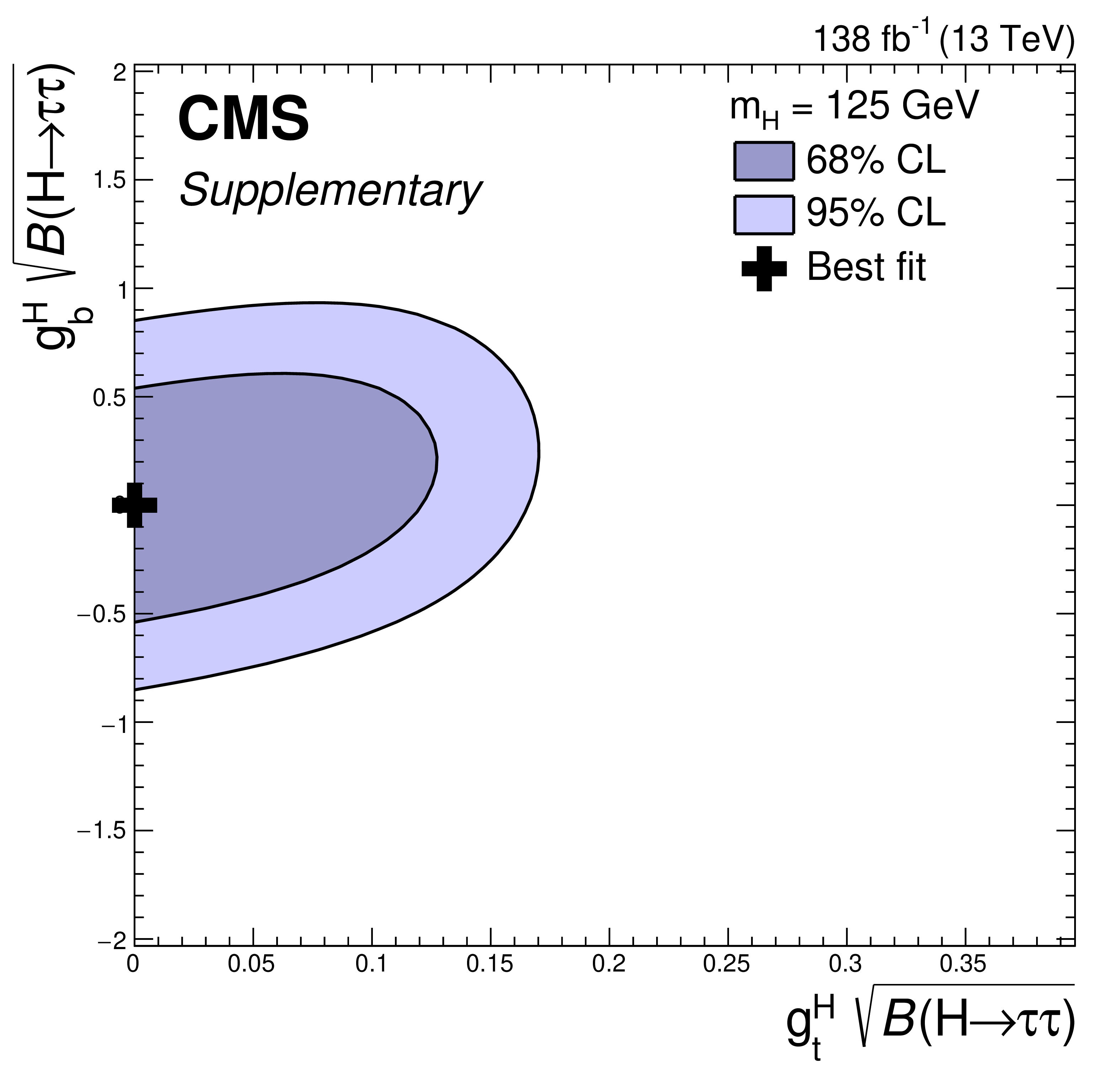
png pdf |
Additional Figure 75:
Maximum likelihood estimate, and 68% and 95% CL contours obtained from scans of the signal-plus-background likelihood for a scalar resonance ($ \mathrm{H} $) with $m_{\mathrm{H}}= $ 125 GeV, produced via $ \mathrm{g} \mathrm{g} \mathrm{H}$ or $ \mathrm{b} \mathrm{b} \mathrm{H}$. For this scan, we assume that both processes are only influenced by the Yukawa couplings to t and b quarks and scale the predicted cross sections depending on these couplings. The estimates are shown for the product of the reduced Yukawa couplings $\mathrm{g}_{ \mathrm{t} ,\, \mathrm{b} }^{\mathrm{H}}$ and $\sqrt{B(\mathrm{H}\to \tau \tau )}$, where the former is defined as the ratio of the Yukawa coupling of $ \mathrm{H} $ over the Yukawa coupling expected for a SM-like Higgs boson of the same mass. An ambiguity on the relative sign of the two couplings can be resolved by the contribution of $ \mathrm{t} \mathrm{b} $-interference terms to the cross section predictions. By convention $\mathrm{g}_{ \mathrm{t} }^{\mathrm{H}}$ has been chosen positive. |
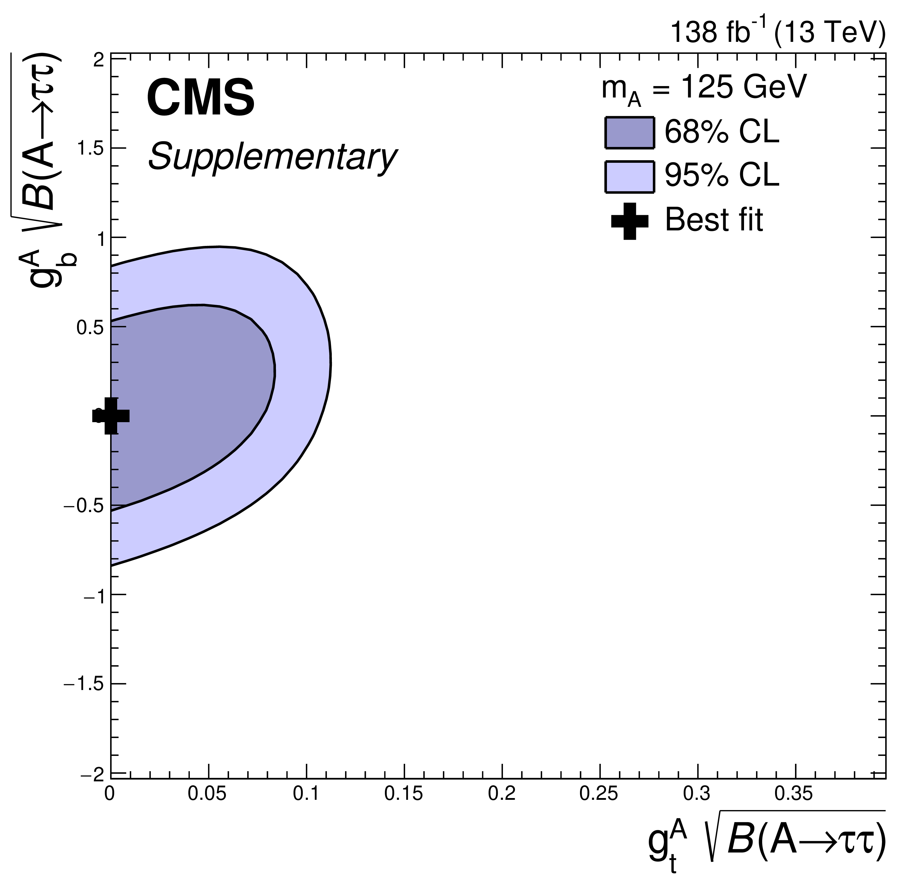
png pdf |
Additional Figure 76:
Maximum likelihood estimate, and 68% and 95% CL contours obtained from scans of the signal-plus-background likelihood for a pseudoscalar resonance ($\mathrm{A}$) with $m_{\mathrm{A}}= $ 125 GeV, produced via $ \mathrm{g} \mathrm{g} \mathrm{A}$ or $ \mathrm{b} \mathrm{b} \mathrm{A}$. For this scan, we assume that both processes are only influenced by the Yukawa couplings to t and b quarks and scale the predicted cross sections depending on these couplings. The estimates are shown for the product of the reduced Yukawa couplings $\mathrm{g}_{ \mathrm{t} ,\, \mathrm{b} }^{\mathrm{A}}$ and $\sqrt{B(\mathrm{A}\to \tau \tau )}$, where the former is defined as the ratio of the Yukawa coupling of $\mathrm{A}$ over the Yukawa coupling expected for a SM-like Higgs boson of the same mass. An ambiguity on the relative sign of the two couplings can be resolved by the contribution of $ \mathrm{t} \mathrm{b} $-interference terms to the cross section predictions. By convention $\mathrm{g}_{ \mathrm{t} }^{\mathrm{A}}$ has been chosen positive. |

png pdf |
Additional Figure 77:
Maximum likelihood estimate, and 68% and 95% CL contours obtained from scans of the signal-plus-background likelihood for a scalar resonance ($ \mathrm{H} $) with $m_{\mathrm{H}}= $ 130 GeV, produced via $ \mathrm{g} \mathrm{g} \mathrm{H}$ or $ \mathrm{b} \mathrm{b} \mathrm{H}$. For this scan, we assume that both processes are only influenced by the Yukawa couplings to t and b quarks and scale the predicted cross sections depending on these couplings. The estimates are shown for the product of the reduced Yukawa couplings $\mathrm{g}_{ \mathrm{t} ,\, \mathrm{b} }^{\mathrm{H}}$ and $\sqrt{B(\mathrm{H}\to \tau \tau )}$, where the former is defined as the ratio of the Yukawa coupling of $ \mathrm{H} $ over the Yukawa coupling expected for a SM-like Higgs boson of the same mass. An ambiguity on the relative sign of the two couplings can be resolved by the contribution of $ \mathrm{t} \mathrm{b} $-interference terms to the cross section predictions. By convention $\mathrm{g}_{ \mathrm{t} }^{\mathrm{H}}$ has been chosen positive. |
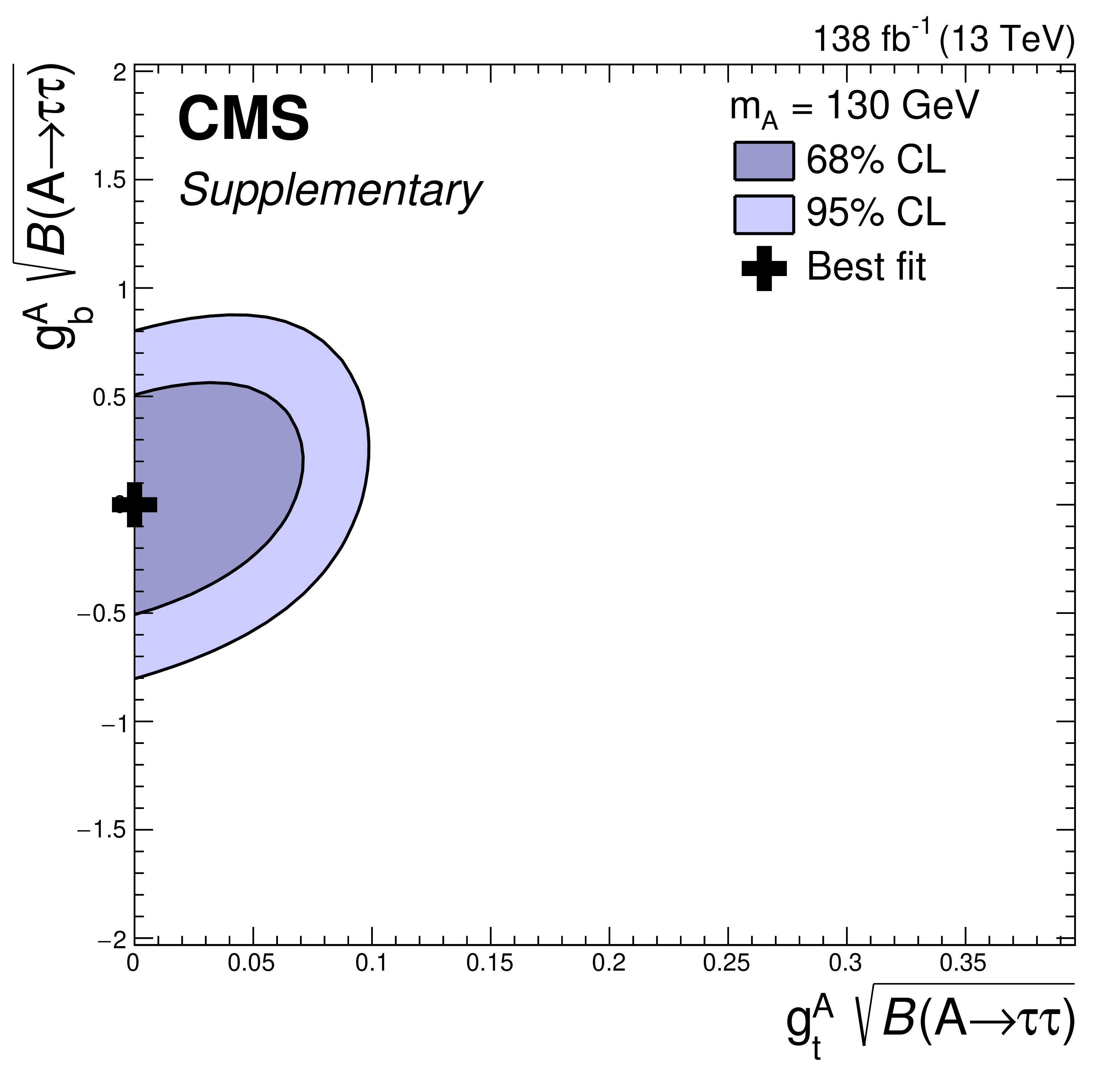
png pdf |
Additional Figure 78:
Maximum likelihood estimate, and 68% and 95% CL contours obtained from scans of the signal-plus-background likelihood for a pseudoscalar resonance ($\mathrm{A}$) with $m_{\mathrm{A}}= $ 130 GeV, produced via $ \mathrm{g} \mathrm{g} \mathrm{A}$ or $ \mathrm{b} \mathrm{b} \mathrm{A}$. For this scan, we assume that both processes are only influenced by the Yukawa couplings to t and b quarks and scale the predicted cross sections depending on these couplings. The estimates are shown for the product of the reduced Yukawa couplings $\mathrm{g}_{ \mathrm{t} ,\, \mathrm{b} }^{\mathrm{A}}$ and $\sqrt{B(\mathrm{A}\to \tau \tau )}$, where the former is defined as the ratio of the Yukawa coupling of $\mathrm{A}$ over the Yukawa coupling expected for a SM-like Higgs boson of the same mass. An ambiguity on the relative sign of the two couplings can be resolved by the contribution of $ \mathrm{t} \mathrm{b} $-interference terms to the cross section predictions. By convention $\mathrm{g}_{ \mathrm{t} }^{\mathrm{A}}$ has been chosen positive. |
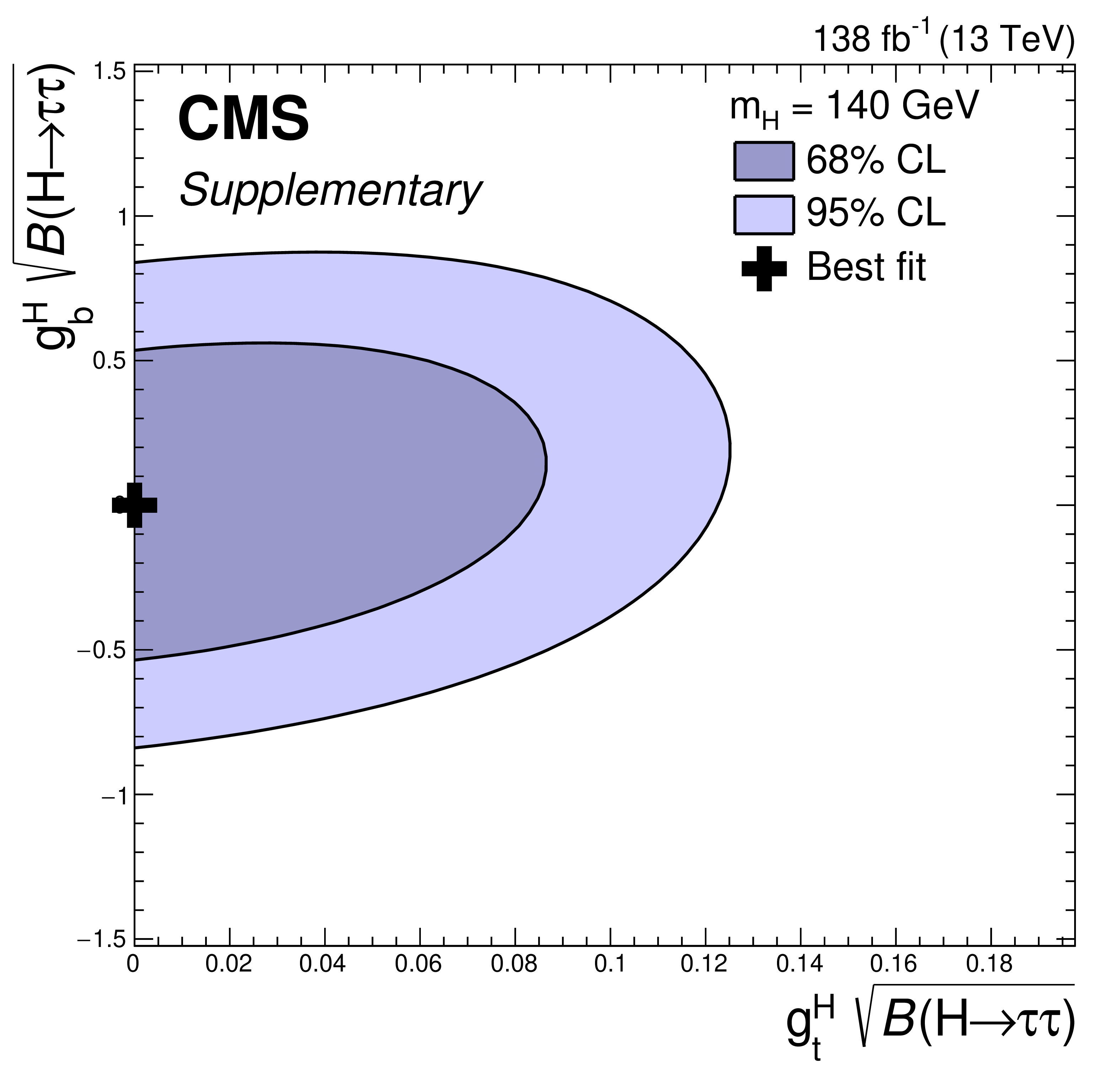
png pdf |
Additional Figure 79:
Maximum likelihood estimate, and 68% and 95% CL contours obtained from scans of the signal-plus-background likelihood for a scalar resonance ($ \mathrm{H} $) with $m_{\mathrm{H}}= $ 140 GeV, produced via $ \mathrm{g} \mathrm{g} \mathrm{H}$ or $ \mathrm{b} \mathrm{b} \mathrm{H}$. For this scan, we assume that both processes are only influenced by the Yukawa couplings to t and b quarks and scale the predicted cross sections depending on these couplings. The estimates are shown for the product of the reduced Yukawa couplings $\mathrm{g}_{ \mathrm{t} ,\, \mathrm{b} }^{\mathrm{H}}$ and $\sqrt{B(\mathrm{H}\to \tau \tau )}$, where the former is defined as the ratio of the Yukawa coupling of $ \mathrm{H} $ over the Yukawa coupling expected for a SM-like Higgs boson of the same mass. An ambiguity on the relative sign of the two couplings can be resolved by the contribution of $ \mathrm{t} \mathrm{b} $-interference terms to the cross section predictions. By convention $\mathrm{g}_{ \mathrm{t} }^{\mathrm{H}}$ has been chosen positive. |
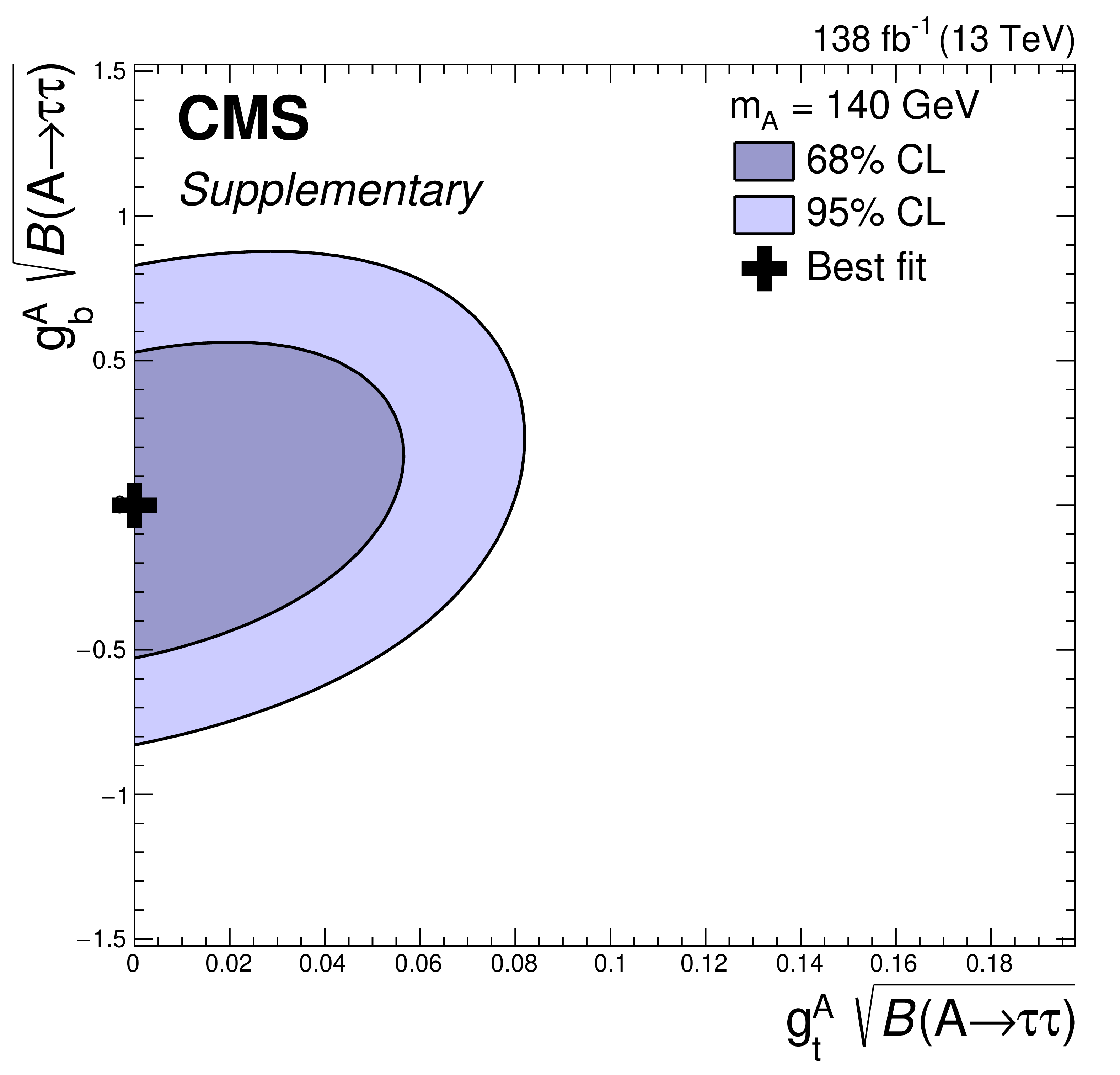
png pdf |
Additional Figure 80:
Maximum likelihood estimate, and 68% and 95% CL contours obtained from scans of the signal-plus-background likelihood for a pseudoscalar resonance ($\mathrm{A}$) with $m_{\mathrm{A}}= $ 140 GeV, produced via $ \mathrm{g} \mathrm{g} \mathrm{A}$ or $ \mathrm{b} \mathrm{b} \mathrm{A}$. For this scan, we assume that both processes are only influenced by the Yukawa couplings to t and b quarks and scale the predicted cross sections depending on these couplings. The estimates are shown for the product of the reduced Yukawa couplings $\mathrm{g}_{ \mathrm{t} ,\, \mathrm{b} }^{\mathrm{A}}$ and $\sqrt{B(\mathrm{A}\to \tau \tau )}$, where the former is defined as the ratio of the Yukawa coupling of $\mathrm{A}$ over the Yukawa coupling expected for a SM-like Higgs boson of the same mass. An ambiguity on the relative sign of the two couplings can be resolved by the contribution of $ \mathrm{t} \mathrm{b} $-interference terms to the cross section predictions. By convention $\mathrm{g}_{ \mathrm{t} }^{\mathrm{A}}$ has been chosen positive. |
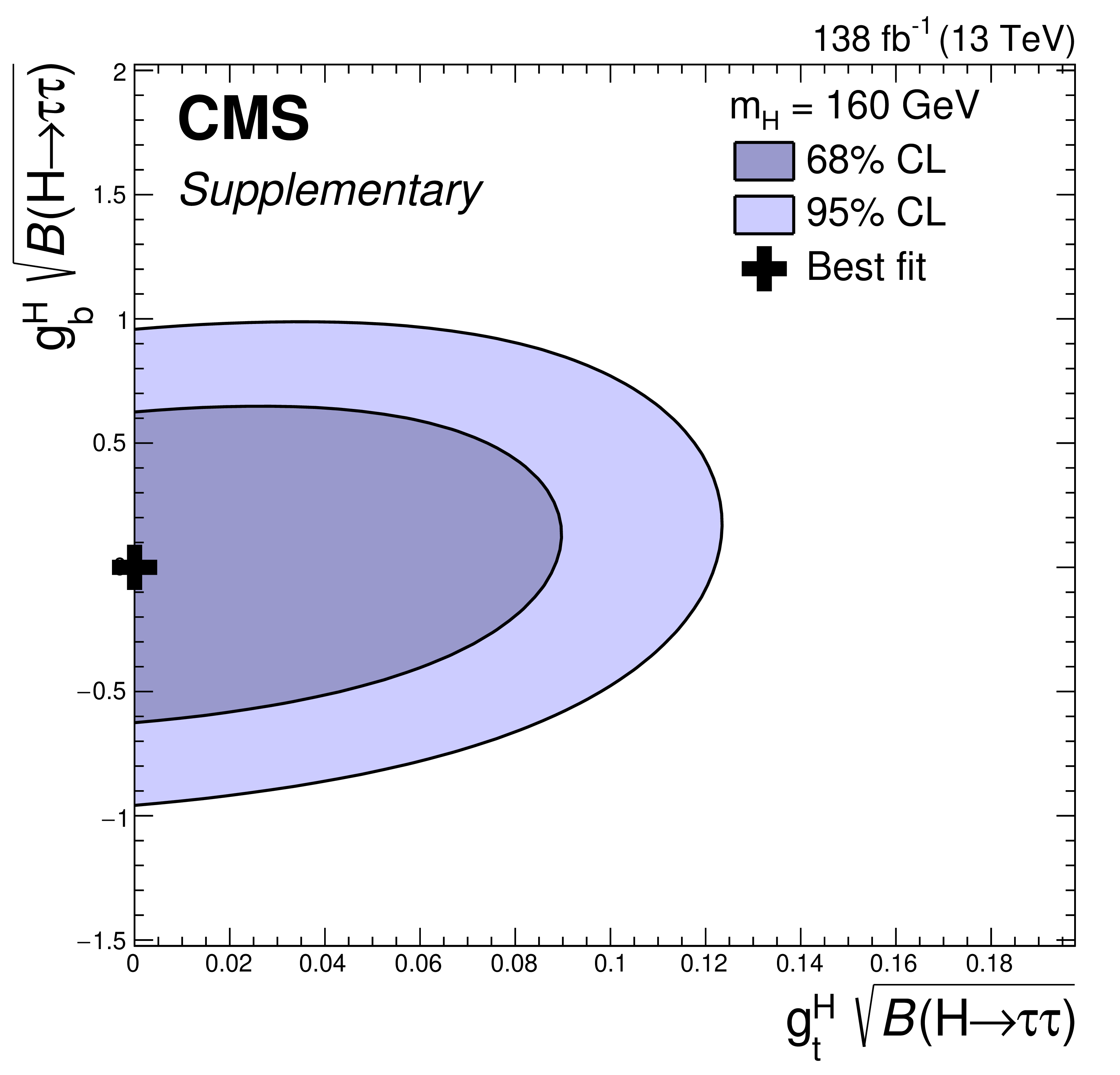
png pdf |
Additional Figure 81:
Maximum likelihood estimate, and 68% and 95% CL contours obtained from scans of the signal-plus-background likelihood for a scalar resonance ($ \mathrm{H} $) with $m_{\mathrm{H}}= $ 160 GeV, produced via $ \mathrm{g} \mathrm{g} \mathrm{H}$ or $ \mathrm{b} \mathrm{b} \mathrm{H}$. For this scan, we assume that both processes are only influenced by the Yukawa couplings to t and b quarks and scale the predicted cross sections depending on these couplings. The estimates are shown for the product of the reduced Yukawa couplings $\mathrm{g}_{ \mathrm{t} ,\, \mathrm{b} }^{\mathrm{H}}$ and $\sqrt{B(\mathrm{H}\to \tau \tau )}$, where the former is defined as the ratio of the Yukawa coupling of $ \mathrm{H} $ over the Yukawa coupling expected for a SM-like Higgs boson of the same mass. An ambiguity on the relative sign of the two couplings can be resolved by the contribution of $ \mathrm{t} \mathrm{b} $-interference terms to the cross section predictions. By convention $\mathrm{g}_{ \mathrm{t} }^{\mathrm{H}}$ has been chosen positive. |
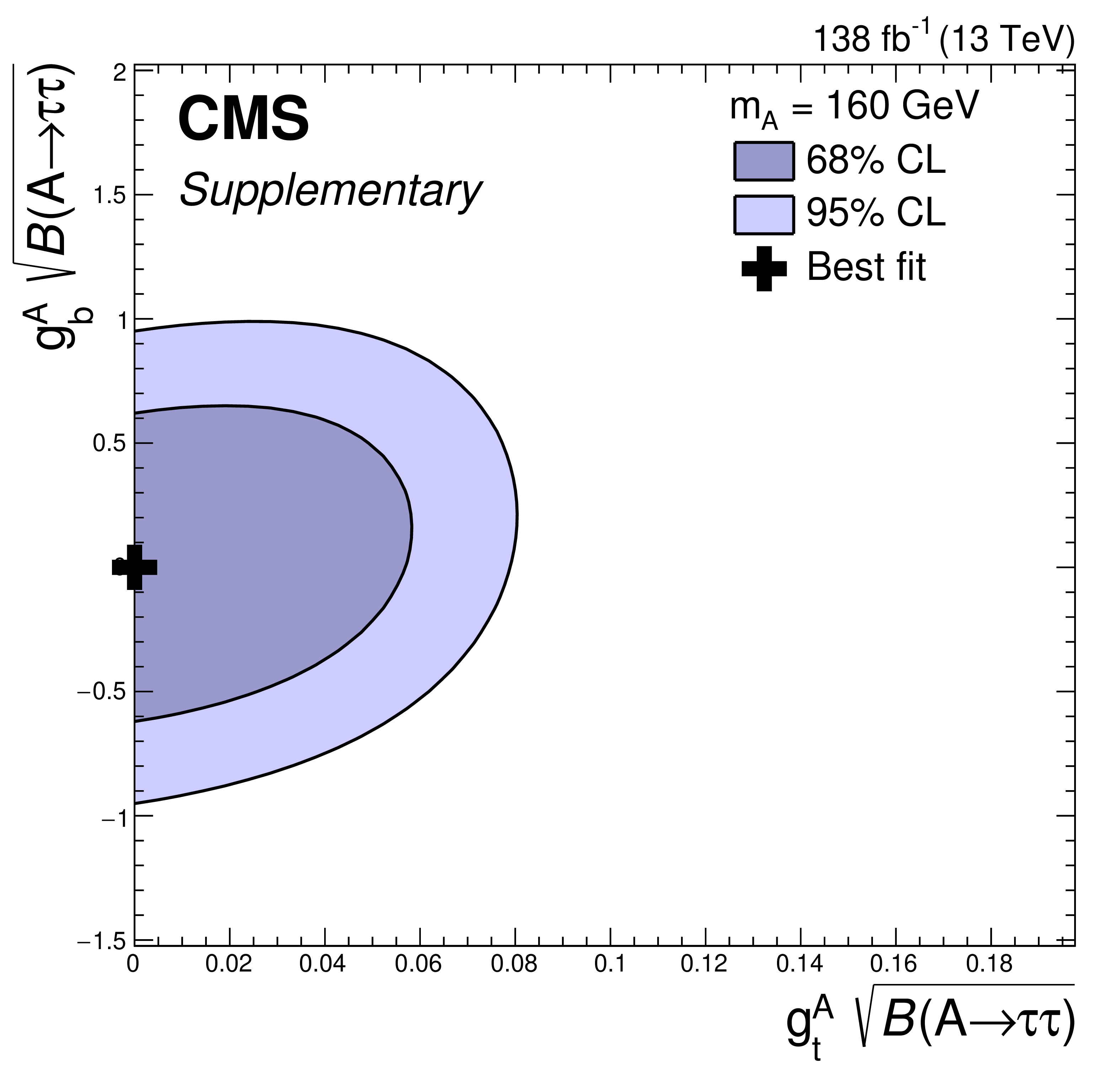
png pdf |
Additional Figure 82:
Maximum likelihood estimate, and 68% and 95% CL contours obtained from scans of the signal-plus-background likelihood for a pseudoscalar resonance ($\mathrm{A}$) with $m_{\mathrm{A}}= $ 160 GeV, produced via $ \mathrm{g} \mathrm{g} \mathrm{A}$ or $ \mathrm{b} \mathrm{b} \mathrm{A}$. For this scan, we assume that both processes are only influenced by the Yukawa couplings to t and b quarks and scale the predicted cross sections depending on these couplings. The estimates are shown for the product of the reduced Yukawa couplings $\mathrm{g}_{ \mathrm{t} ,\, \mathrm{b} }^{\mathrm{A}}$ and $\sqrt{B(\mathrm{A}\to \tau \tau )}$, where the former is defined as the ratio of the Yukawa coupling of $\mathrm{A}$ over the Yukawa coupling expected for a SM-like Higgs boson of the same mass. An ambiguity on the relative sign of the two couplings can be resolved by the contribution of $ \mathrm{t} \mathrm{b} $-interference terms to the cross section predictions. By convention $\mathrm{g}_{ \mathrm{t} }^{\mathrm{A}}$ has been chosen positive. |

png pdf |
Additional Figure 83:
Maximum likelihood estimate, and 68% and 95% CL contours obtained from scans of the signal-plus-background likelihood for a scalar resonance ($ \mathrm{H} $) with $m_{\mathrm{H}}= $ 180 GeV, produced via $ \mathrm{g} \mathrm{g} \mathrm{H}$ or $ \mathrm{b} \mathrm{b} \mathrm{H}$. For this scan, we assume that both processes are only influenced by the Yukawa couplings to t and b quarks and scale the predicted cross sections depending on these couplings. The estimates are shown for the product of the reduced Yukawa couplings $\mathrm{g}_{ \mathrm{t} ,\, \mathrm{b} }^{\mathrm{H}}$ and $\sqrt{B(\mathrm{H}\to \tau \tau )}$, where the former is defined as the ratio of the Yukawa coupling of $ \mathrm{H} $ over the Yukawa coupling expected for a SM-like Higgs boson of the same mass. An ambiguity on the relative sign of the two couplings can be resolved by the contribution of $ \mathrm{t} \mathrm{b} $-interference terms to the cross section predictions. By convention $\mathrm{g}_{ \mathrm{t} }^{\mathrm{H}}$ has been chosen positive. |
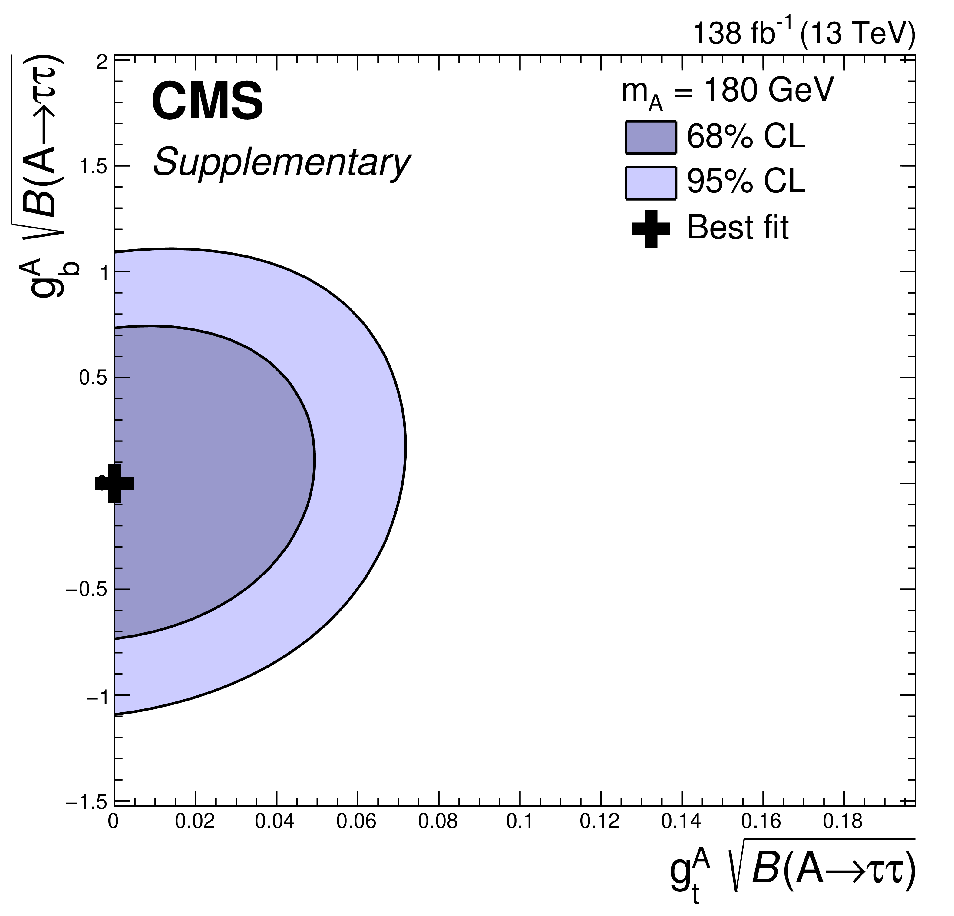
png pdf |
Additional Figure 84:
Maximum likelihood estimate, and 68% and 95% CL contours obtained from scans of the signal-plus-background likelihood for a pseudoscalar resonance ($\mathrm{A}$) with $m_{\mathrm{A}}= $ 180 GeV, produced via $ \mathrm{g} \mathrm{g} \mathrm{A}$ or $ \mathrm{b} \mathrm{b} \mathrm{A}$. For this scan, we assume that both processes are only influenced by the Yukawa couplings to t and b quarks and scale the predicted cross sections depending on these couplings. The estimates are shown for the product of the reduced Yukawa couplings $\mathrm{g}_{ \mathrm{t} ,\, \mathrm{b} }^{\mathrm{A}}$ and $\sqrt{B(\mathrm{A}\to \tau \tau )}$, where the former is defined as the ratio of the Yukawa coupling of $\mathrm{A}$ over the Yukawa coupling expected for a SM-like Higgs boson of the same mass. An ambiguity on the relative sign of the two couplings can be resolved by the contribution of $ \mathrm{t} \mathrm{b} $-interference terms to the cross section predictions. By convention $\mathrm{g}_{ \mathrm{t} }^{\mathrm{A}}$ has been chosen positive. |
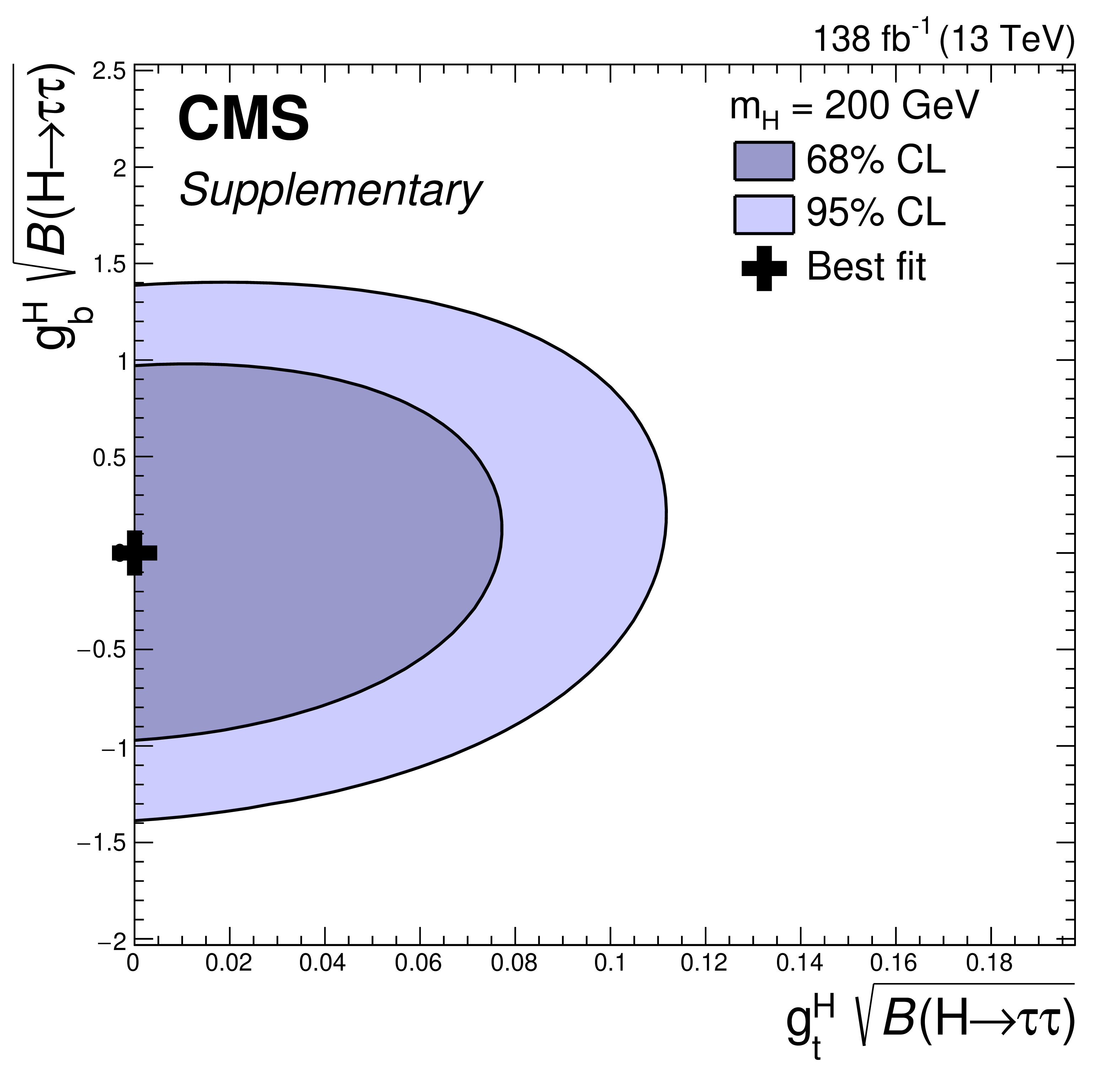
png pdf |
Additional Figure 85:
Maximum likelihood estimate, and 68% and 95% CL contours obtained from scans of the signal-plus-background likelihood for a scalar resonance ($ \mathrm{H} $) with $m_{\mathrm{H}}= $ 200 GeV, produced via $ \mathrm{g} \mathrm{g} \mathrm{H}$ or $ \mathrm{b} \mathrm{b} \mathrm{H}$. For this scan, we assume that both processes are only influenced by the Yukawa couplings to t and b quarks and scale the predicted cross sections depending on these couplings. The estimates are shown for the product of the reduced Yukawa couplings $\mathrm{g}_{ \mathrm{t} ,\, \mathrm{b} }^{\mathrm{H}}$ and $\sqrt{B(\mathrm{H}\to \tau \tau )}$, where the former is defined as the ratio of the Yukawa coupling of $ \mathrm{H} $ over the Yukawa coupling expected for a SM-like Higgs boson of the same mass. An ambiguity on the relative sign of the two couplings can be resolved by the contribution of $ \mathrm{t} \mathrm{b} $-interference terms to the cross section predictions. By convention $\mathrm{g}_{ \mathrm{t} }^{\mathrm{H}}$ has been chosen positive. |
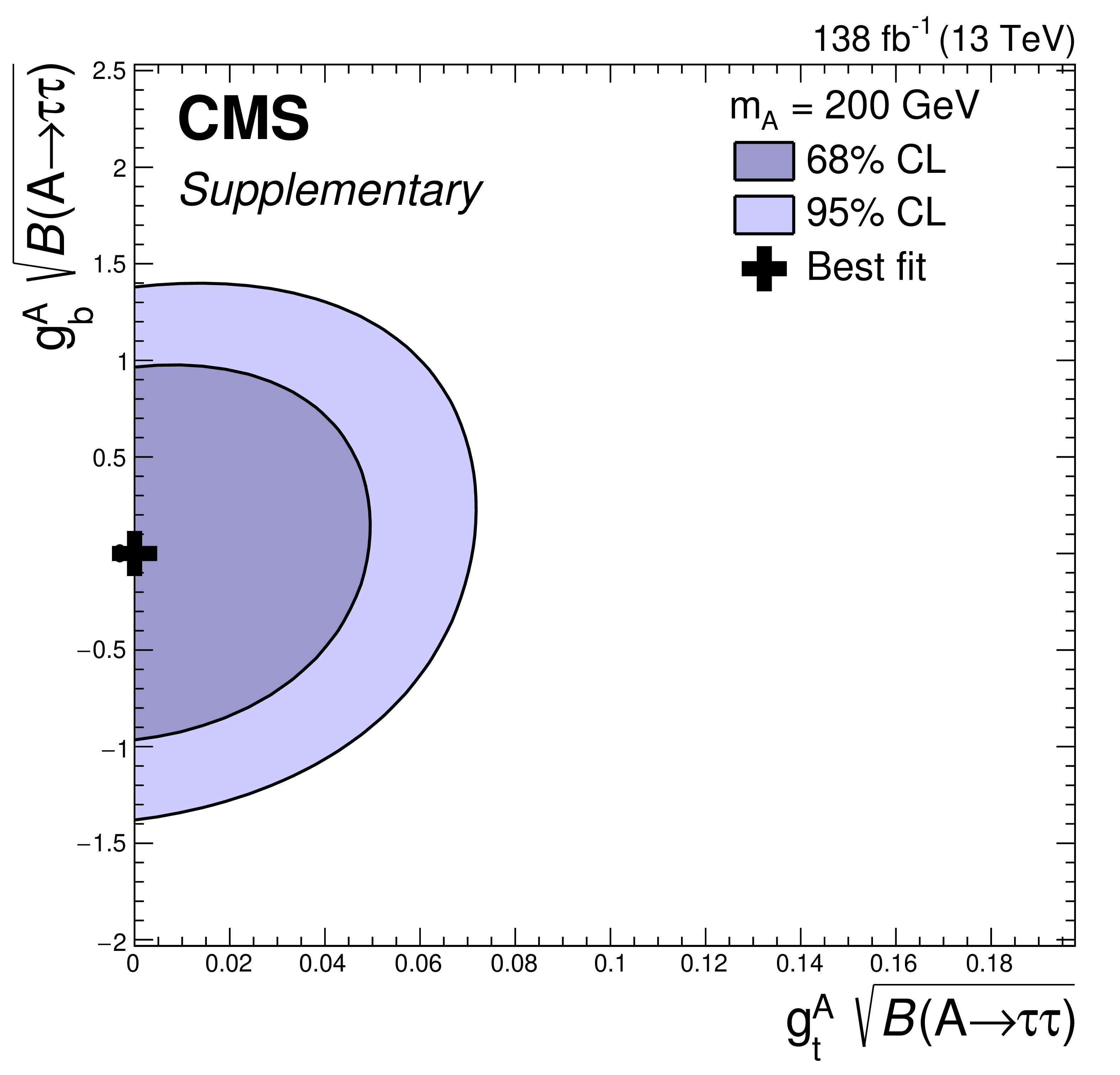
png pdf |
Additional Figure 86:
Maximum likelihood estimate, and 68% and 95% CL contours obtained from scans of the signal-plus-background likelihood for a pseudoscalar resonance ($\mathrm{A}$) with $m_{\mathrm{A}}= $ 200 GeV, produced via $ \mathrm{g} \mathrm{g} \mathrm{A}$ or $ \mathrm{b} \mathrm{b} \mathrm{A}$. For this scan, we assume that both processes are only influenced by the Yukawa couplings to t and b quarks and scale the predicted cross sections depending on these couplings. The estimates are shown for the product of the reduced Yukawa couplings $\mathrm{g}_{ \mathrm{t} ,\, \mathrm{b} }^{\mathrm{A}}$ and $\sqrt{B(\mathrm{A}\to \tau \tau )}$, where the former is defined as the ratio of the Yukawa coupling of $\mathrm{A}$ over the Yukawa coupling expected for a SM-like Higgs boson of the same mass. An ambiguity on the relative sign of the two couplings can be resolved by the contribution of $ \mathrm{t} \mathrm{b} $-interference terms to the cross section predictions. By convention $\mathrm{g}_{ \mathrm{t} }^{\mathrm{A}}$ has been chosen positive. |

png pdf |
Additional Figure 87:
Best fit values of $\sigma( \mathrm{g} \mathrm{g} \phi)B(\phi\to \tau \tau )$ split by data-taking year compared to the fit result obtained from all data-taking years combined, for $m_{\phi}= $ 1.2 TeV. A test of the compatibility of the fit results from each data-taking year individually across all data-taking years exhibits a $p$-value of 64%. |
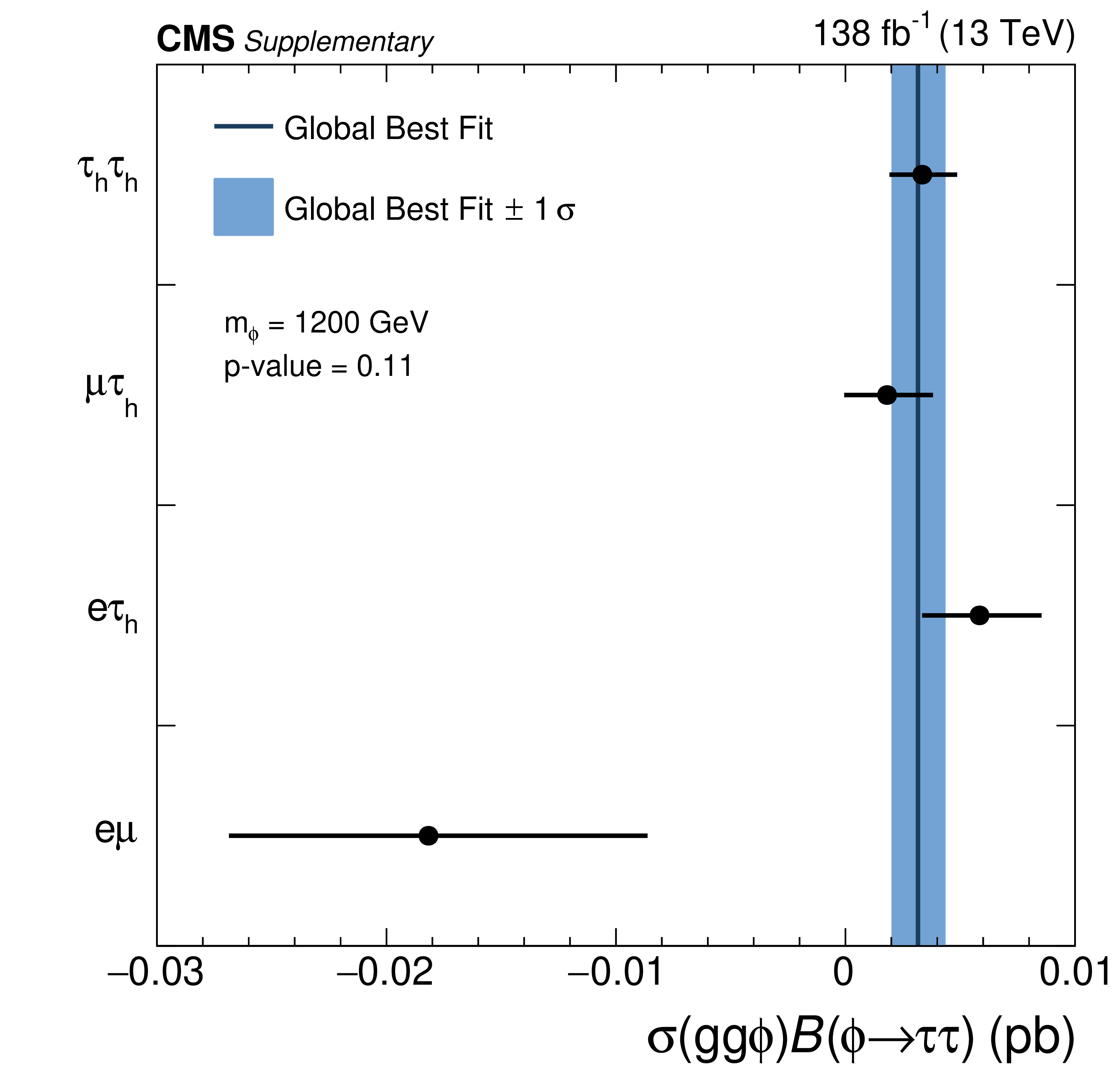
png pdf |
Additional Figure 88:
Best fit values of $\sigma( \mathrm{g} \mathrm{g} \phi)B(\phi\to \tau \tau )$ split by $ \tau \tau $ final state compared to the fit result obtained from all $ \tau \tau $ final states combined, for $m_{\phi}= $ 1.2 TeV. A test of the compatibility of the fit results in each $ \tau \tau $ final state individually across all $ \tau \tau $ final states exhibits a $p$-value of 11%. |

png pdf |
Additional Figure 89:
Best fit values of $\sigma( \mathrm{g} \mathrm{g} \phi)B(\phi\to \tau \tau )$ split by data-taking year compared to the fit result obtained from all data-taking years combined, for $m_{\phi}= $ 100 GeV. A test of the compatibility of the fit results from each data-taking year individually across all data-taking years exhibits a $p$-value of 58%. |
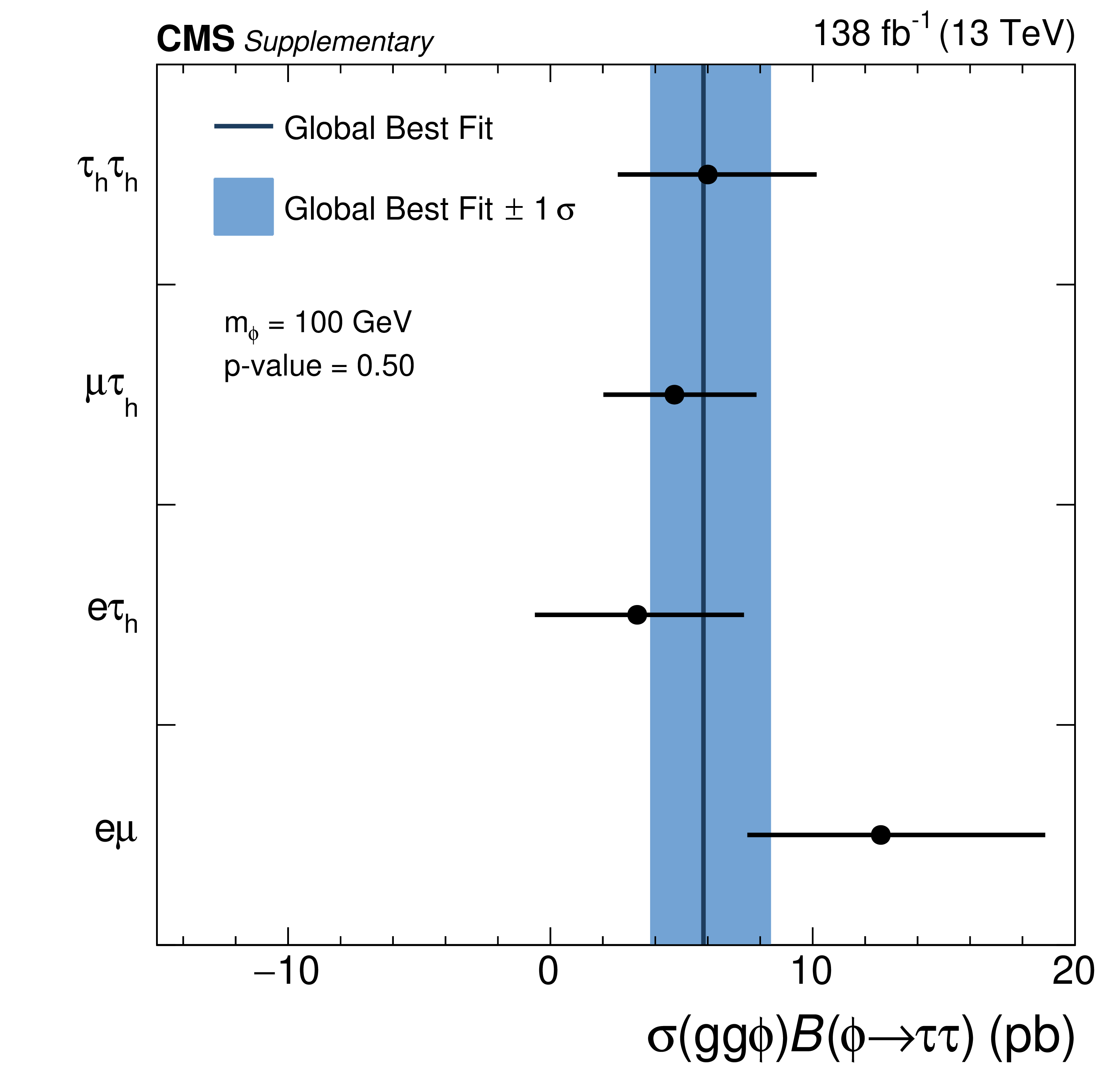
png pdf |
Additional Figure 90:
Best fit values of $\sigma( \mathrm{g} \mathrm{g} \phi)B(\phi\to \tau \tau )$ split by $ \tau \tau $ final state compared to the fit result obtained from all $ \tau \tau $ final states combined, for $m_{\phi}= $ 100 GeV. A test of the compatibility of the fit results in each $ \tau \tau $ final state individually across all $ \tau \tau $ final states exhibits a $p$-value of 50%. |
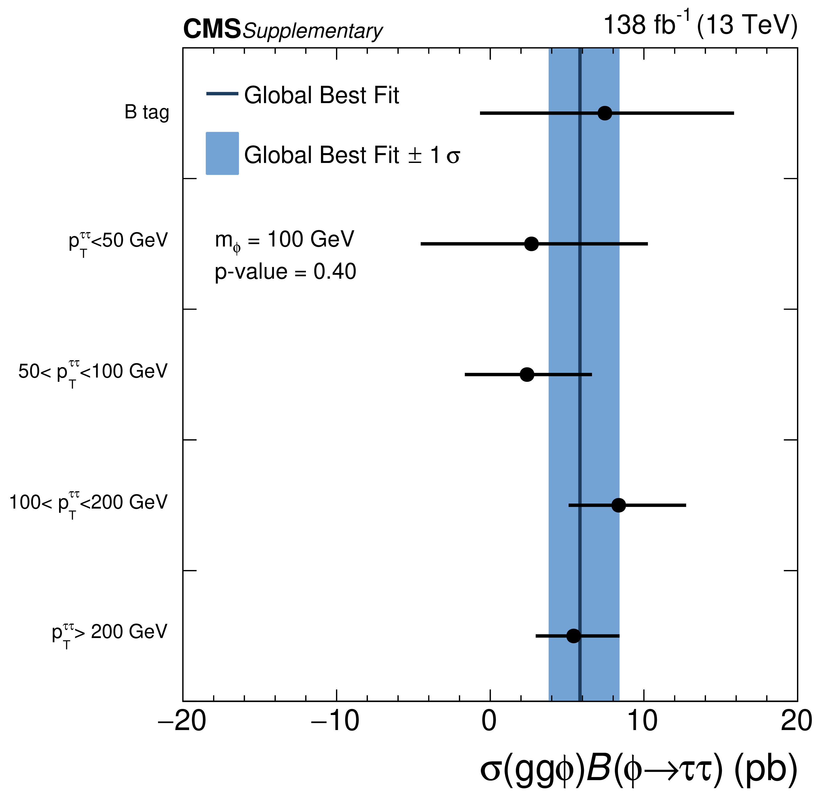
png pdf |
Additional Figure 91:
Best fit values of $\sigma( \mathrm{g} \mathrm{g} \phi)B(\phi\to \tau \tau )$ split by category used for the extraction of the signal compared to the fit result obtained from all categories combined, for $m_{\phi}= $ 100 GeV. A test of the compatibility of the fit results in each category individually across all categories exhibits a $p$-value of 40%. |
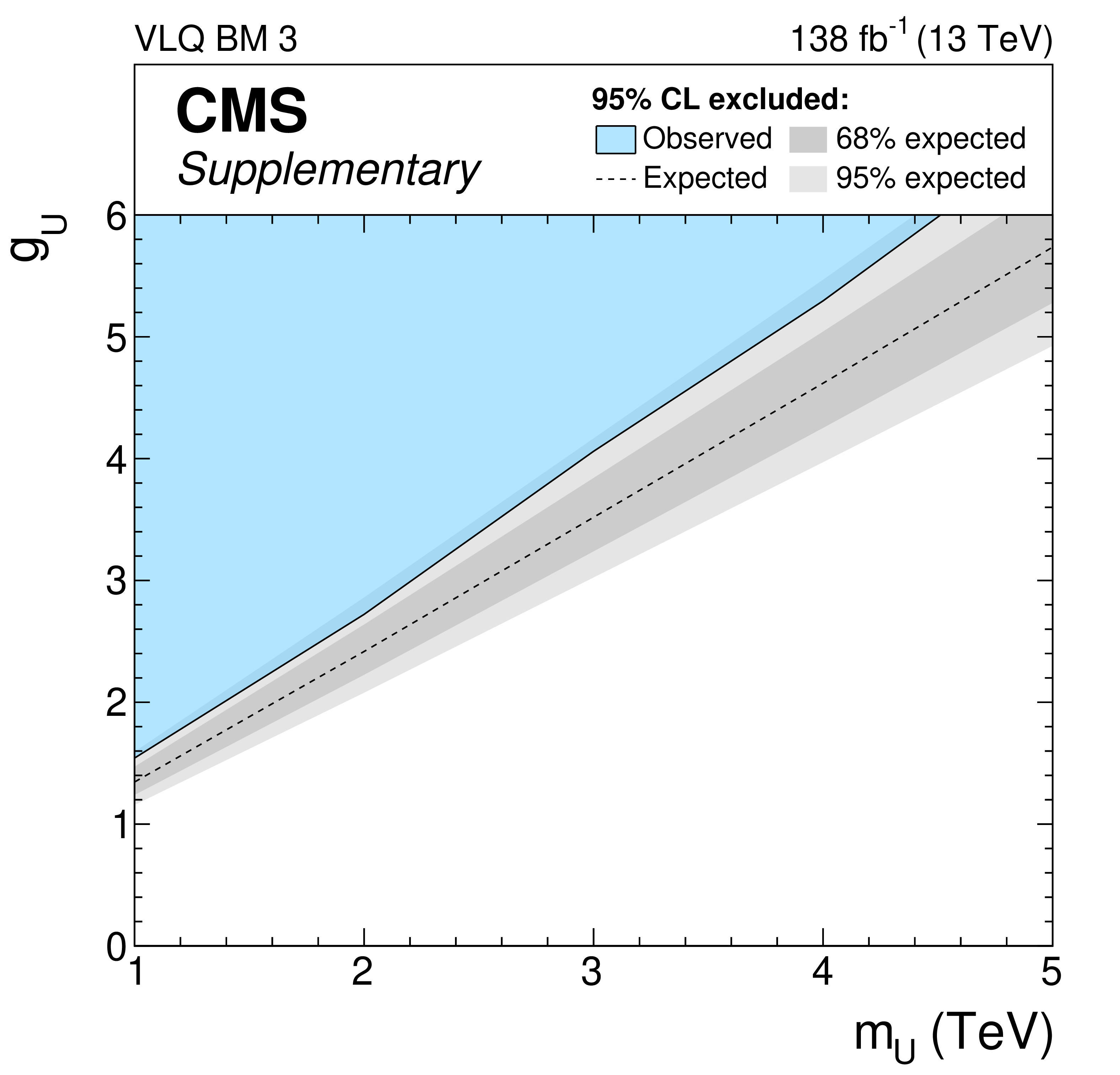
png pdf |
Additional Figure 92:
Expected and observed 95% CL upper limits on $g_{\text{U}}$ in a benchmark scenario in which $\beta_{\mathrm{L}}^{ \mathrm{b} \tau }$ is taken to be 1 and the other couplings are set to zero (labeled as ``VLQ BM 3''), in a mass range of 1 $ \leq m_{\text{U}}\leq $ 5 TeV. The expected median of the exclusion limit in the absence of signal is shown by the dashed line. The dark and bright grey bands indicate the central 68% and 95% intervals of the expected exclusion limit. The observed excluded parameter space is indicated by the coloured blue area. |
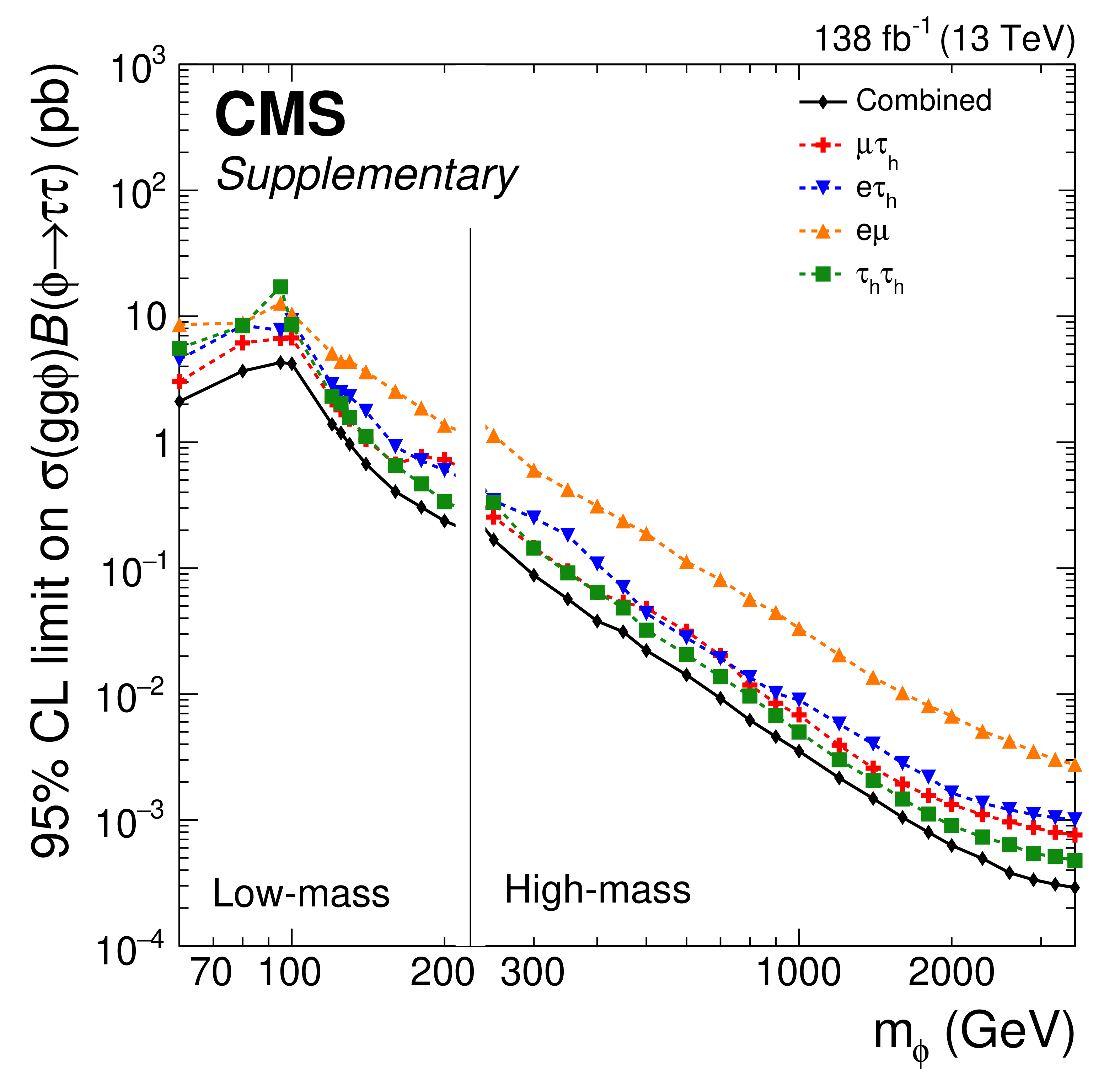
png pdf |
Additional Figure 93:
Expected 95% CL upper limits on $\sigma( \mathrm{g} \mathrm{g} \phi)B(\phi\to \tau \tau )$, in the mass range of 60 $ \leq m_{\phi}\leq $ 3500 GeV, split by $ \tau \tau $ final state. |

png pdf |
Additional Figure 94:
Expected 95% CL upper limits on $\sigma( \mathrm{b} \mathrm{b} \phi)B(\phi\to \tau \tau )$, in the mass range of 60 $ \leq m_{\phi}\leq $ 3500 GeV, split by $ \tau \tau $ final state. |
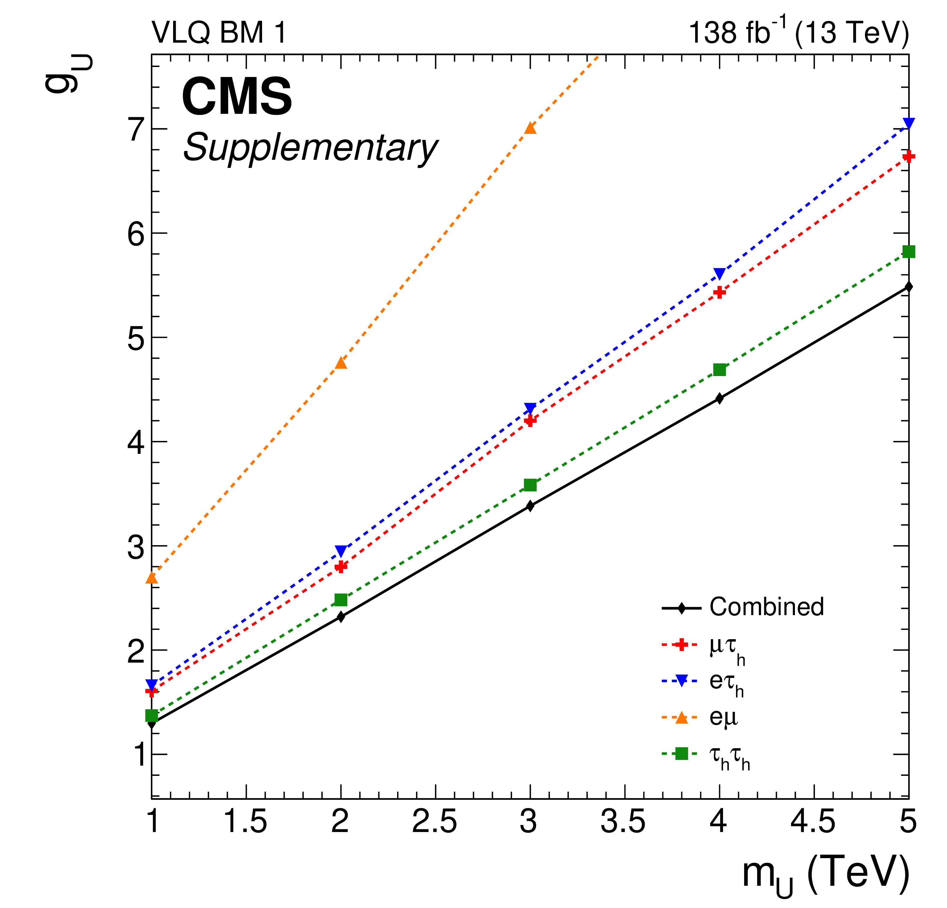
png pdf |
Additional Figure 95:
Expected 95% CL upper limits on $g_{\text{U}}$, in the mass range of 1 $ \leq m_{\text{U}}\leq $ 5 TeV, split by $ \tau \tau $ final state, for the VLQ BM 1 scenario. |
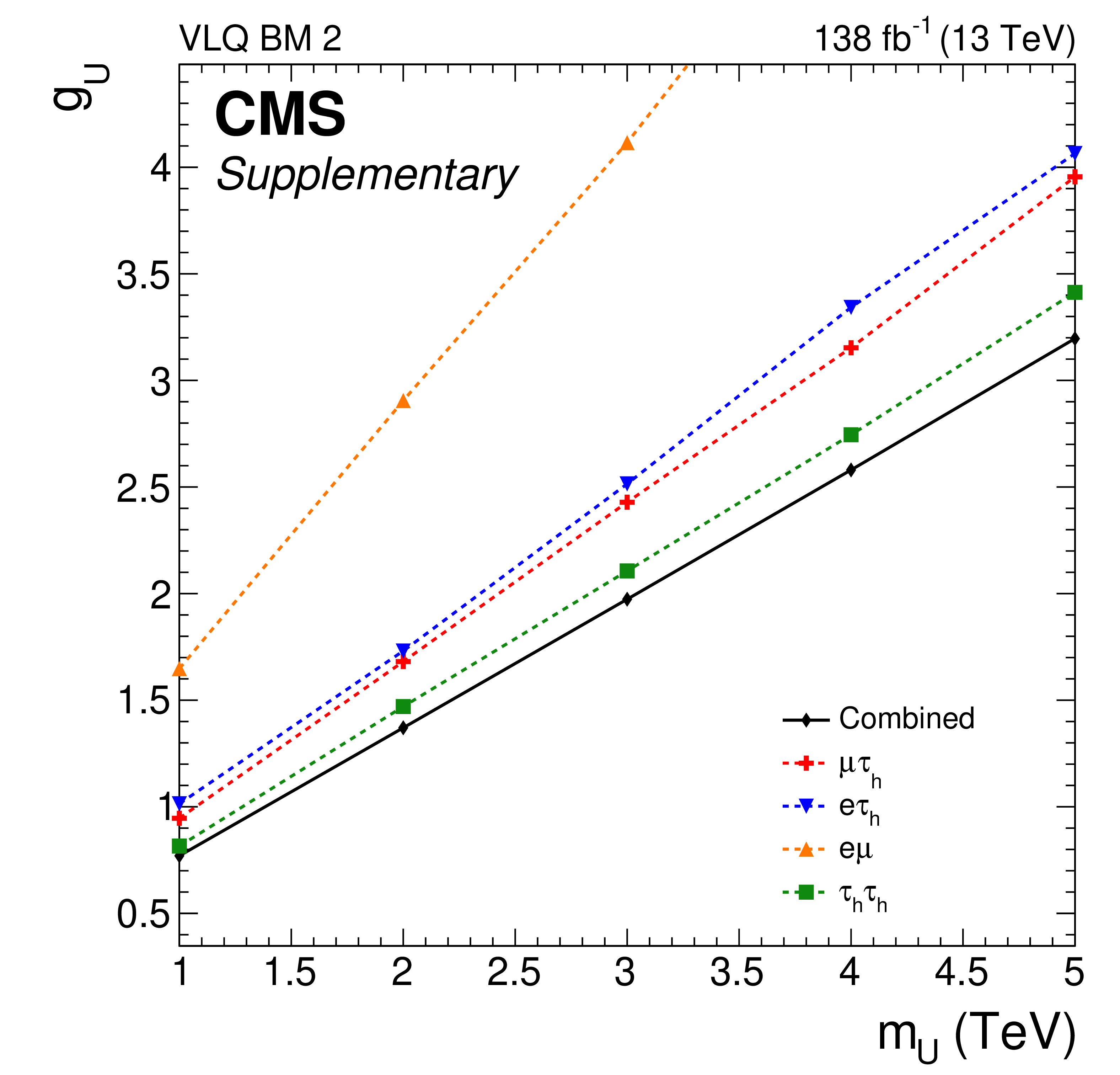
png pdf |
Additional Figure 96:
Expected 95% CL upper limits on $g_{\text{U}}$, in the mass range of 1 $ \leq m_{\text{U}}\leq $ 5 TeV, split by $ \tau \tau $ final state, for the VLQ BM 2 scenario. |
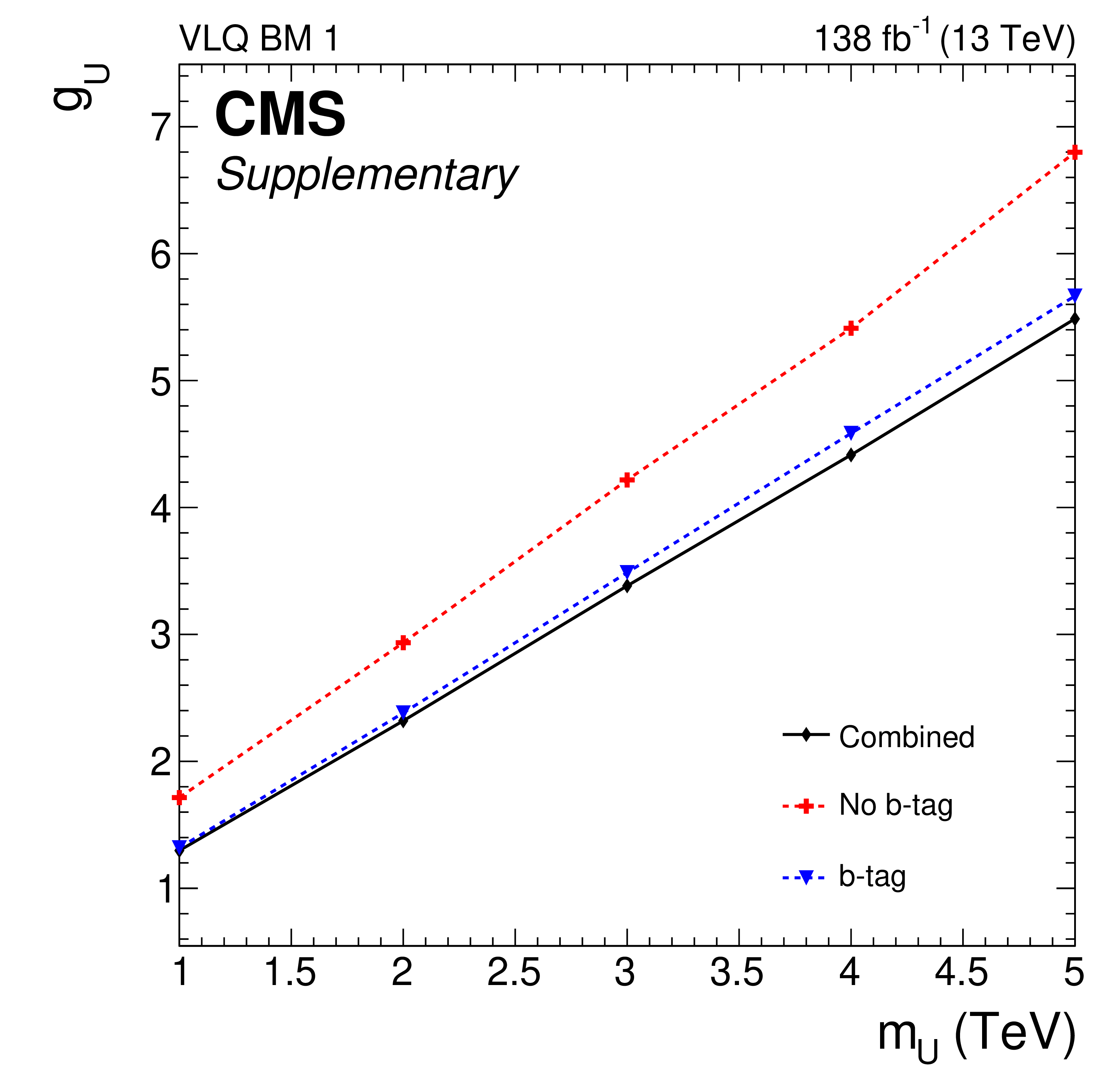
png pdf |
Additional Figure 97:
Expected 95% CL upper limits on $g_{\text{U}}$, in the mass range of 1 $ \leq m_{\text{U}}\leq $ 5 TeV, split by category used for the extraction of the signal, for the VLQ BM 1 scenario. |
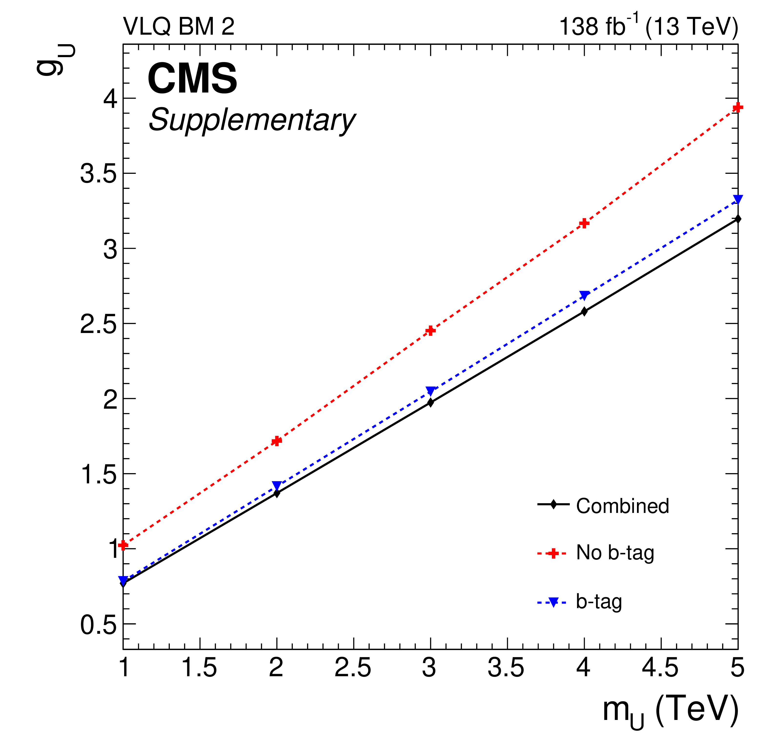
png pdf |
Additional Figure 98:
Expected 95% CL upper limits on $g_{\text{U}}$, in the mass range of 1 $ \leq m_{\text{U}}\leq $ 5 TeV, split by category used for the extraction of the signal, for the VLQ BM 2 scenario. |
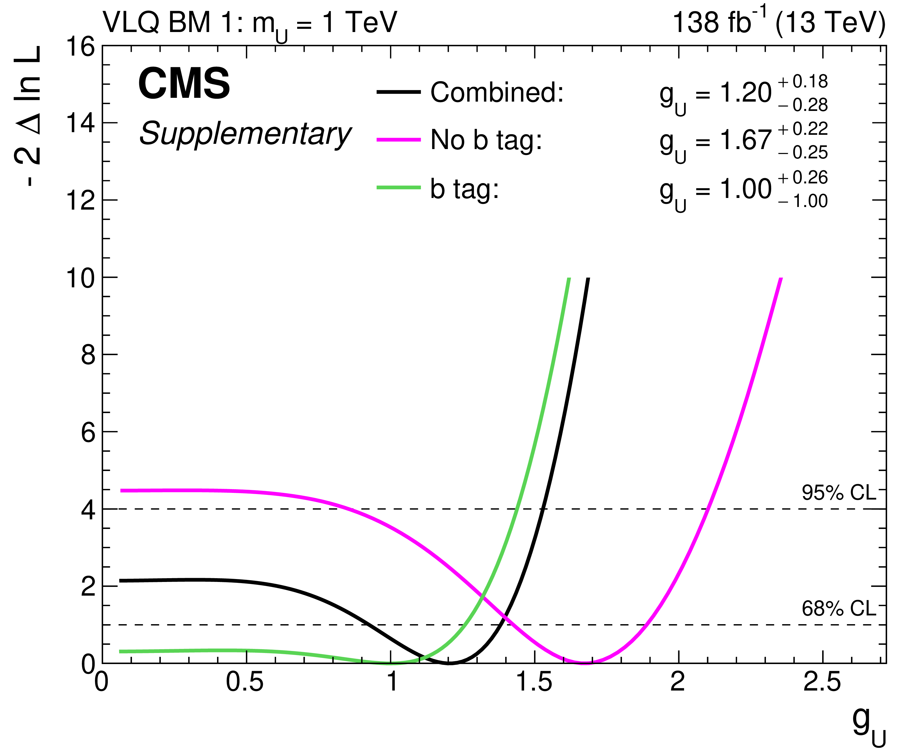
png pdf |
Additional Figure 99:
Scan of the likelihood function for the search for a vector leptoquark with $m_{\text{U}}= $ 1 TeV, in the VLQ BM 1 scenario. This is shown for the cases where the (green) ``b tag'' and (magenta) ``No btag'' categories are fitted separately, and (black) for the fit of both categories combined. |
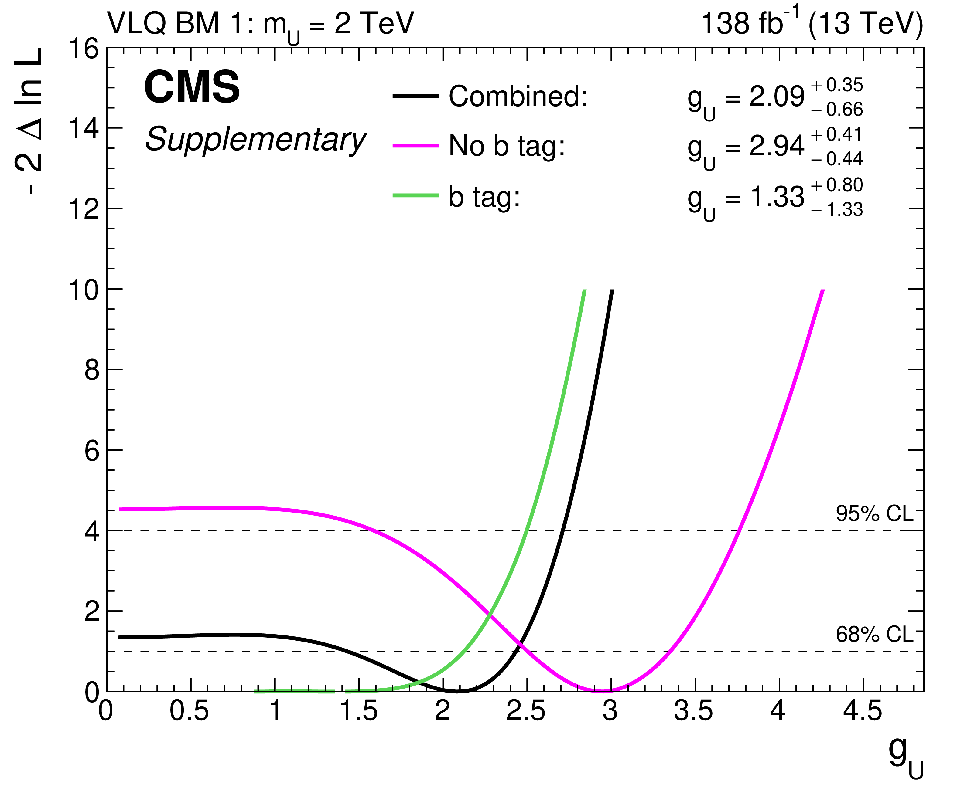
png pdf |
Additional Figure 100:
Scan of the likelihood function for the search for a vector leptoquark with $m_{\text{U}}= $ 1 TeV, in the VLQ BM 1 scenario. This is shown for the cases where the (green) ``b tag'' and (magenta) ``No btag'' categories are fitted separately, and (black) for the fit of both categories combined. |
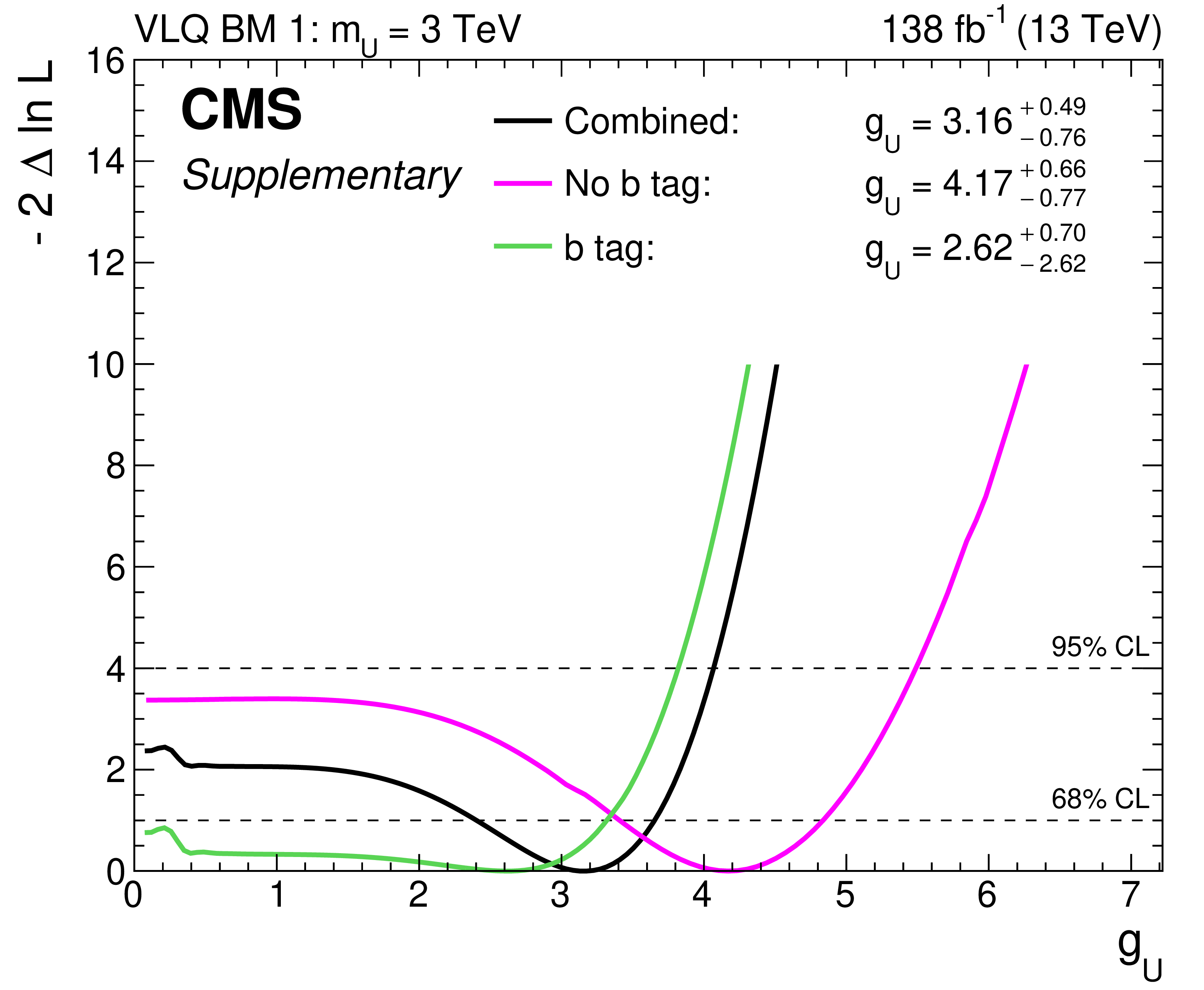
png pdf |
Additional Figure 101:
Scan of the likelihood function for the search for a vector leptoquark with $m_{\text{U}}= $ 3 TeV, in the VLQ BM 1 scenario. This is shown for the cases where the (green) ``b tag'' and (magenta) ``No btag'' categories are fitted separately, and (black) for the fit of both categories combined. |
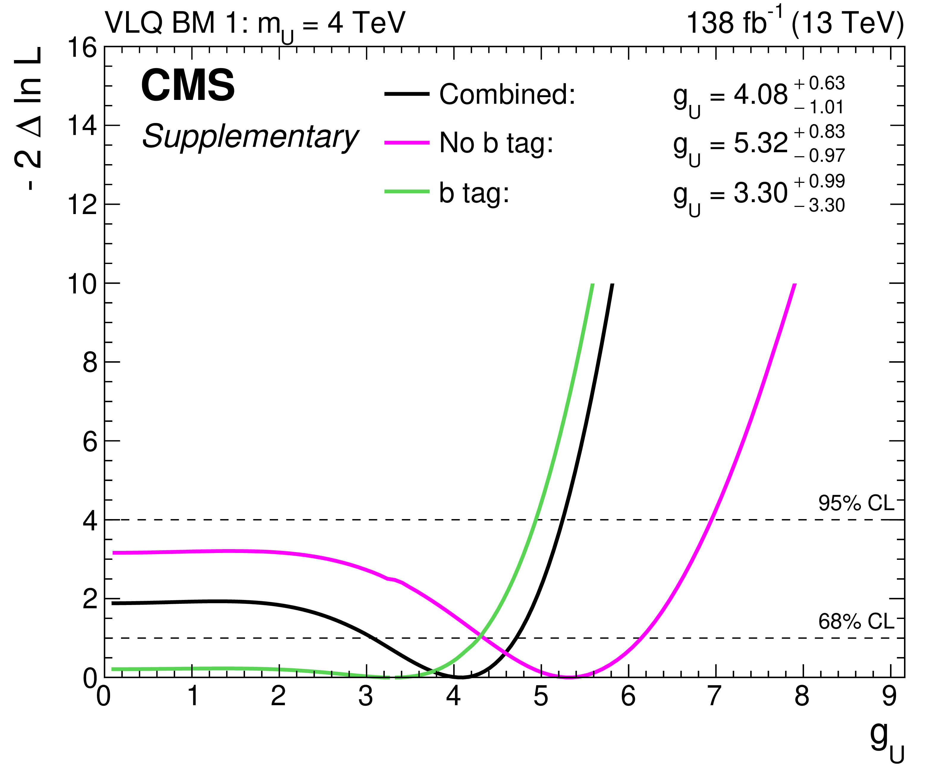
png pdf |
Additional Figure 102:
Scan of the likelihood function for the search for a vector leptoquark with $m_{\text{U}}= $ 4 TeV, in the VLQ BM 1 scenario. This is shown for the cases where the (green) ``b tag'' and (magenta) ``No btag'' categories are fitted separately, and (black) for the fit of both categories combined. |
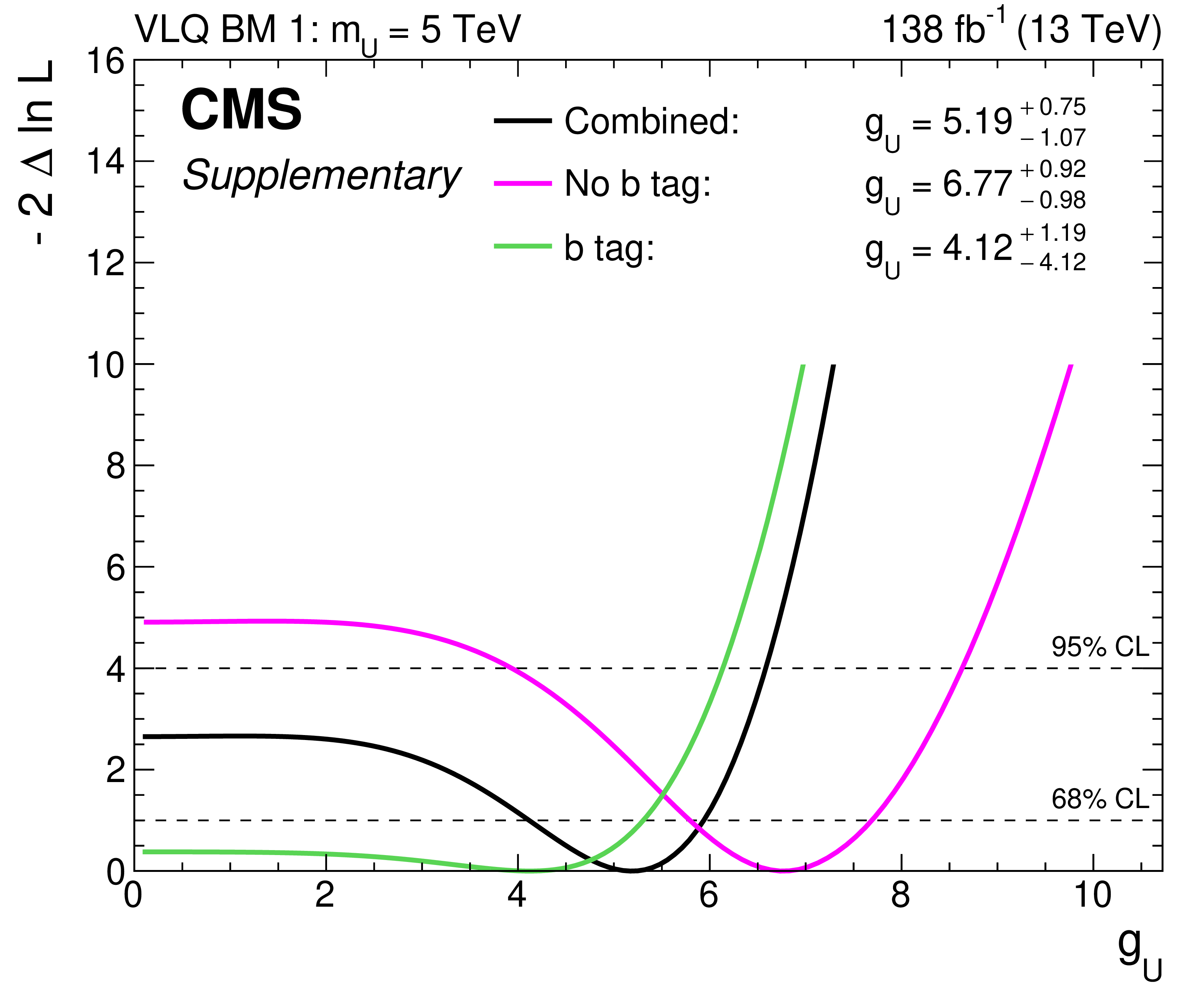
png pdf |
Additional Figure 103:
Scan of the likelihood function for the search for a vector leptoquark with $m_{\text{U}}= $ 5 TeV, in the VLQ BM 1 scenario. This is shown for the cases where the (green) ``b tag'' and (magenta) ``No btag'' categories are fitted separately, and (black) for the fit of both categories combined. |
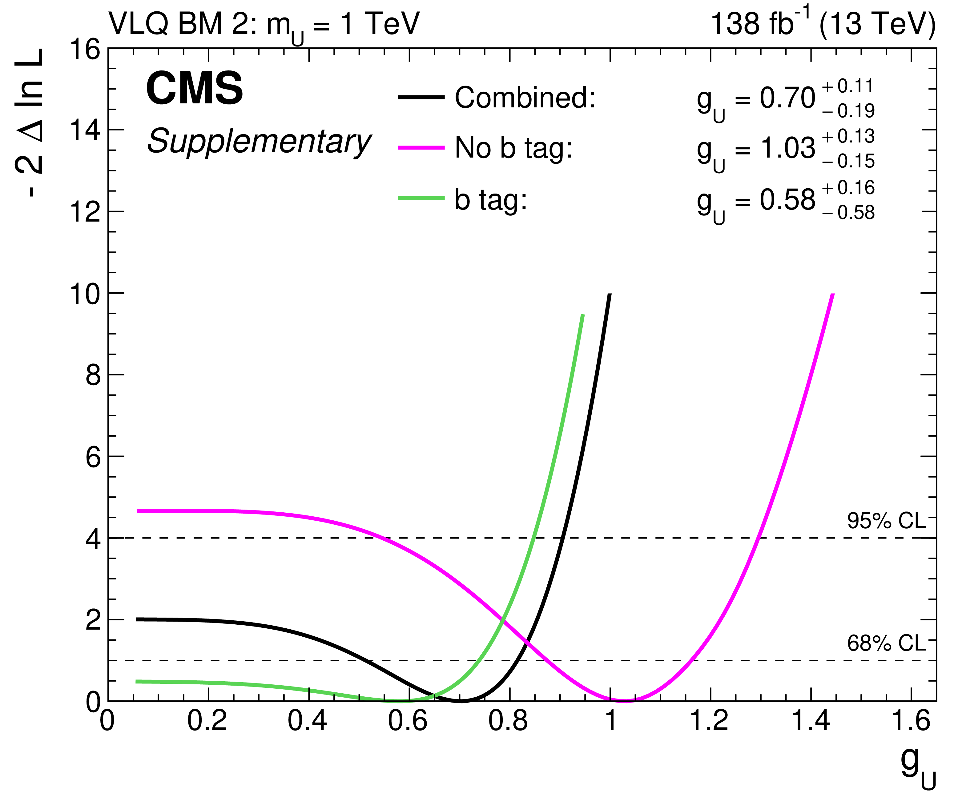
png pdf |
Additional Figure 104:
Scan of the likelihood function for the search for a vector leptoquark with $m_{\text{U}}= $ 1 TeV, in the VLQ BM 2 scenario. This is shown for the cases where the (green) ``b tag'' and (magenta) ``No btag'' categories are fitted separately, and (black) for the fit of both categories combined. |
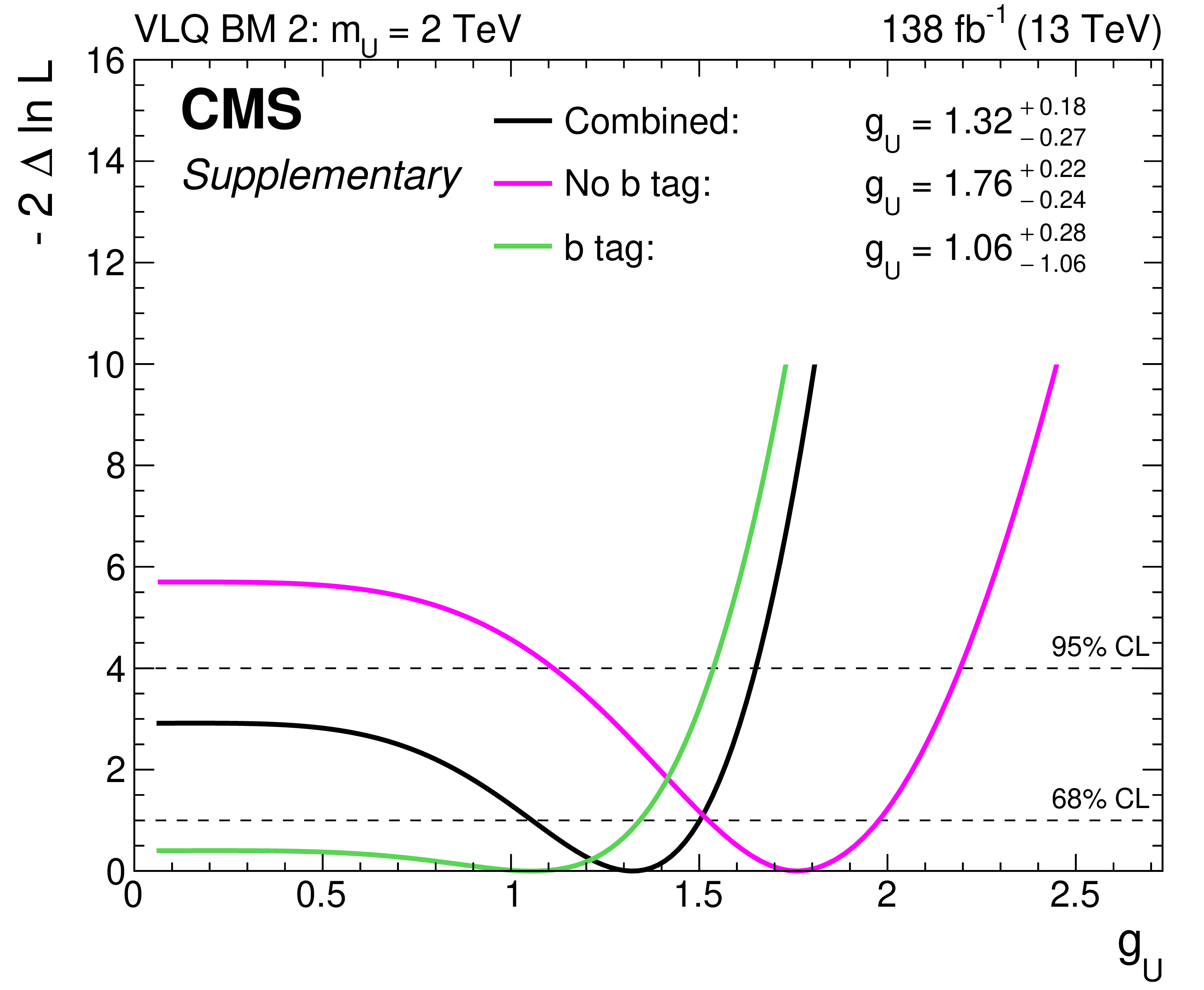
png pdf |
Additional Figure 105:
Scan of the likelihood function for the search for a vector leptoquark with $m_{\text{U}}= $ 2 TeV, in the VLQ BM 2 scenario. This is shown for the cases where the (green) ``b tag'' and (magenta) ``No btag'' categories are fitted separately, and (black) for the fit of both categories combined. |

png pdf |
Additional Figure 106:
Scan of the likelihood function for the search for a vector leptoquark with $m_{\text{U}}= $ 3 TeV, in the VLQ BM 2 scenario. This is shown for the cases where the (green) ``b tag'' and (magenta) ``No btag'' categories are fitted separately, and (black) for the fit of both categories combined. |
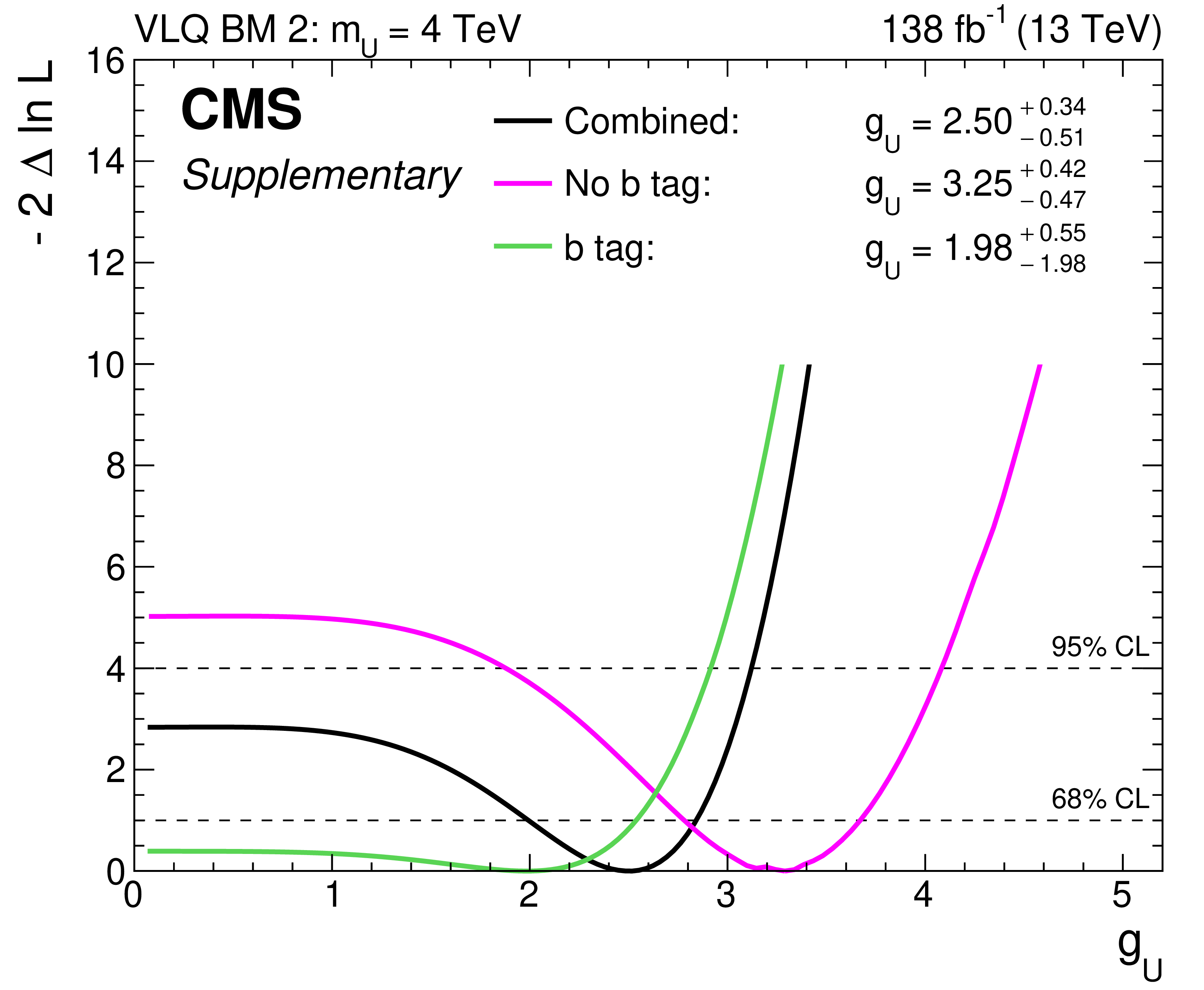
png pdf |
Additional Figure 107:
Scan of the likelihood function for the search for a vector leptoquark with $m_{\text{U}}= $ 4 TeV, in the VLQ BM 2 scenario. This is shown for the cases where the (green) ``b tag'' and (magenta) ``No btag'' categories are fitted separately, and (black) for the fit of both categories combined. |
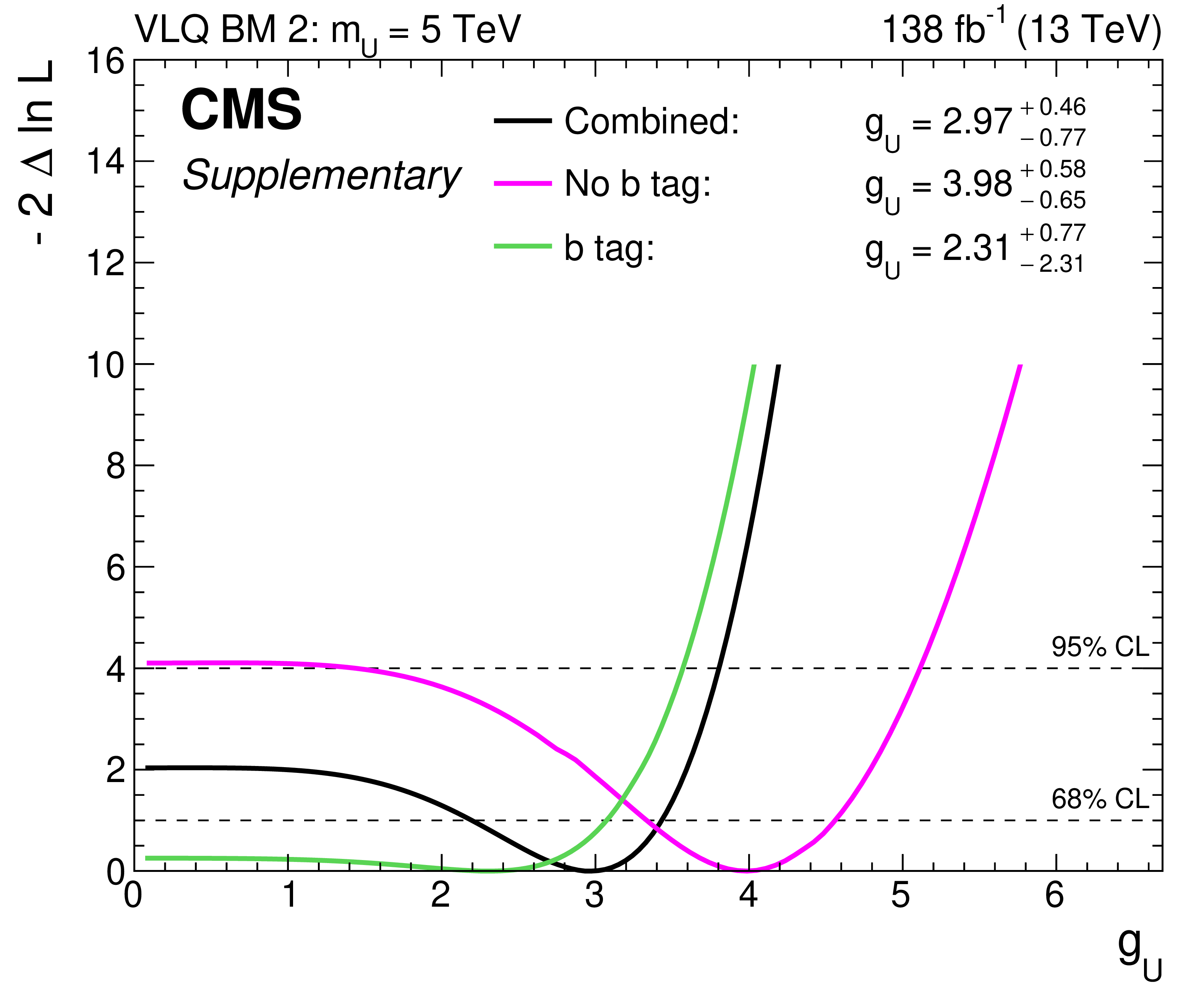
png pdf |
Additional Figure 108:
Scan of the likelihood function for the search for a vector leptoquark with $m_{\text{U}}= $ 5 TeV, in the VLQ BM 2 scenario. This is shown for the cases where the (green) ``b tag'' and (magenta) ``No btag'' categories are fitted separately, and (black) for the fit of both categories combined. |

png pdf |
Additional Figure 109:
Scan of the likelihood function for the search for a vector leptoquark with $m_{\text{U}}= $ 1 TeV, in a benchmark scenario in which $\beta_{\mathrm{L}}^{ \mathrm{b} \tau }$ is taken to be 1 and the other couplings are set to zero (labeled as ``VLQ BM 3''). This is shown for the cases where the (green) ``b tag'' and (magenta) ``No btag'' categories are fitted separately, and (black) for the fit of both categories combined. |
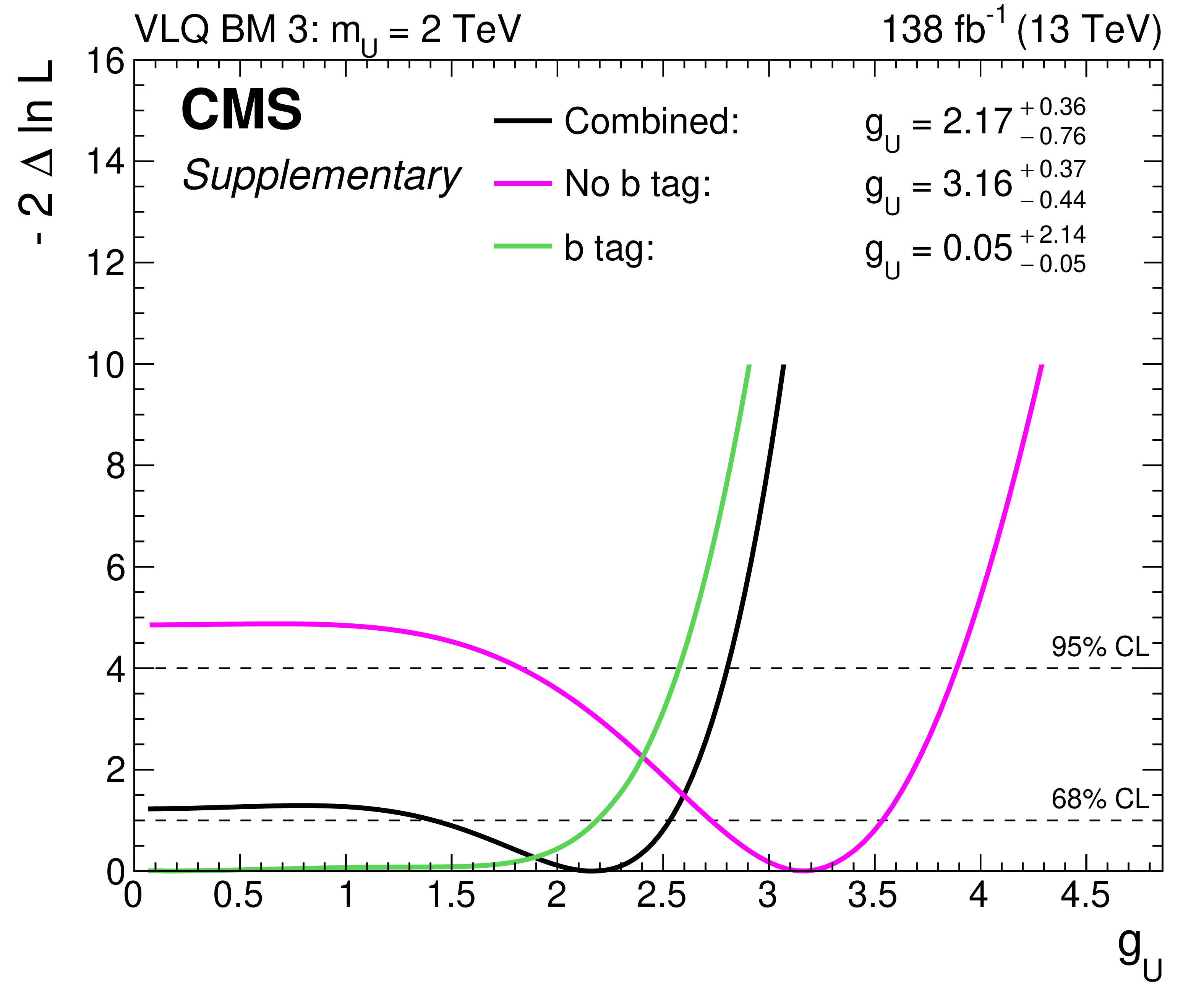
png pdf |
Additional Figure 110:
Scan of the likelihood function for the search for a vector leptoquark with $m_{\text{U}}= $ 2 TeV, in a benchmark scenario in which $\beta_{\mathrm{L}}^{ \mathrm{b} \tau }$ is taken to be 1 and the other couplings are set to zero (labeled as ``VLQ BM 3''). This is shown for the cases where the (green) ``b tag'' and (magenta) ``No btag'' categories are fitted separately, and (black) for the fit of both categories combined. |
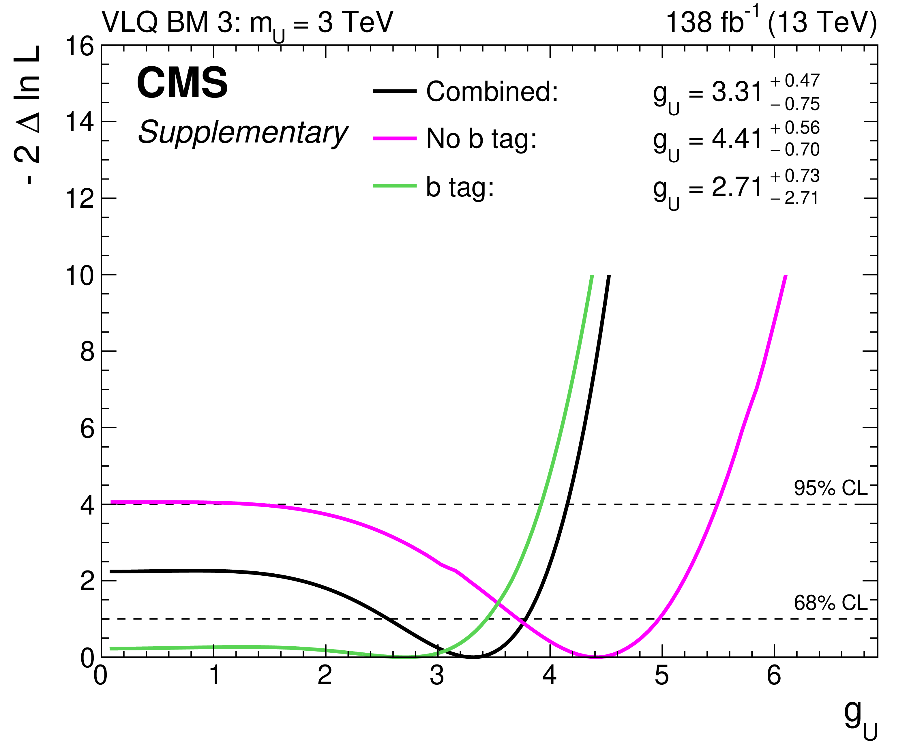
png pdf |
Additional Figure 111:
Scan of the likelihood function for the search for a vector leptoquark with $m_{\text{U}}= $ 3 TeV, in a benchmark scenario in which $\beta_{\mathrm{L}}^{ \mathrm{b} \tau }$ is taken to be 1 and the other couplings are set to zero (labeled as ``VLQ BM 3''). This is shown for the cases where the (green) ``b tag'' and (magenta) ``No btag'' categories are fitted separately, and (black) for the fit of both categories combined. |
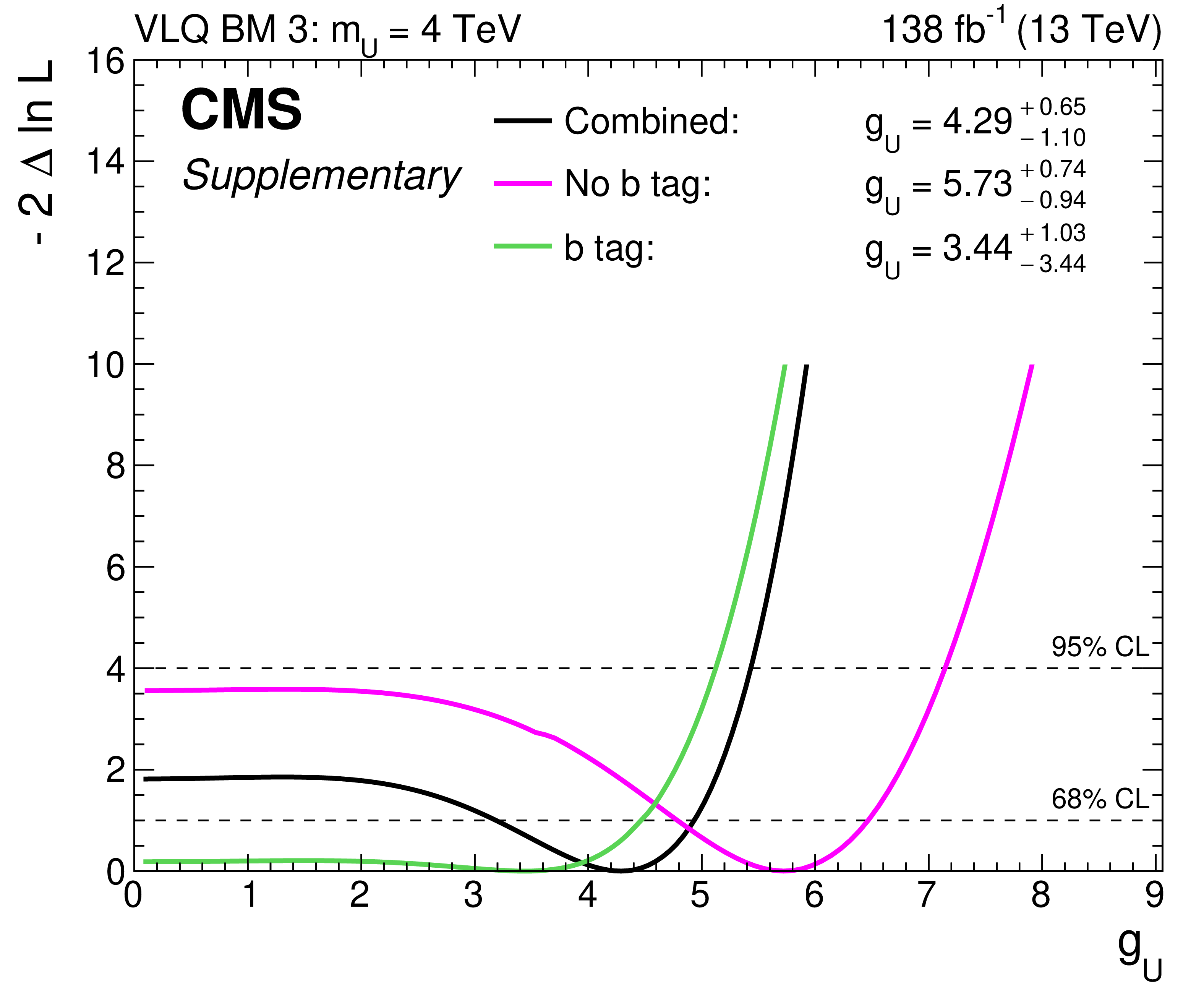
png pdf |
Additional Figure 112:
Scan of the likelihood function for the search for a vector leptoquark with $m_{\text{U}}= $ 4 TeV, in a benchmark scenario in which $\beta_{\mathrm{L}}^{ \mathrm{b} \tau }$ is taken to be 1 and the other couplings are set to zero (labeled as ``VLQ BM 3''). This is shown for the cases where the (green) ``b tag'' and (magenta) ``No btag'' categories are fitted separately, and (black) for the fit of both categories combined. |

png pdf |
Additional Figure 113:
Scan of the likelihood function for the search for a vector leptoquark with $m_{\text{U}}= $ 5 TeV, in a benchmark scenario in which $\beta_{\mathrm{L}}^{ \mathrm{b} \tau }$ is taken to be 1 and the other couplings are set to zero (labeled as ``VLQ BM 3''). This is shown for the cases where the (green) ``b tag'' and (magenta) ``No btag'' categories are fitted separately, and (black) for the fit of both categories combined. |
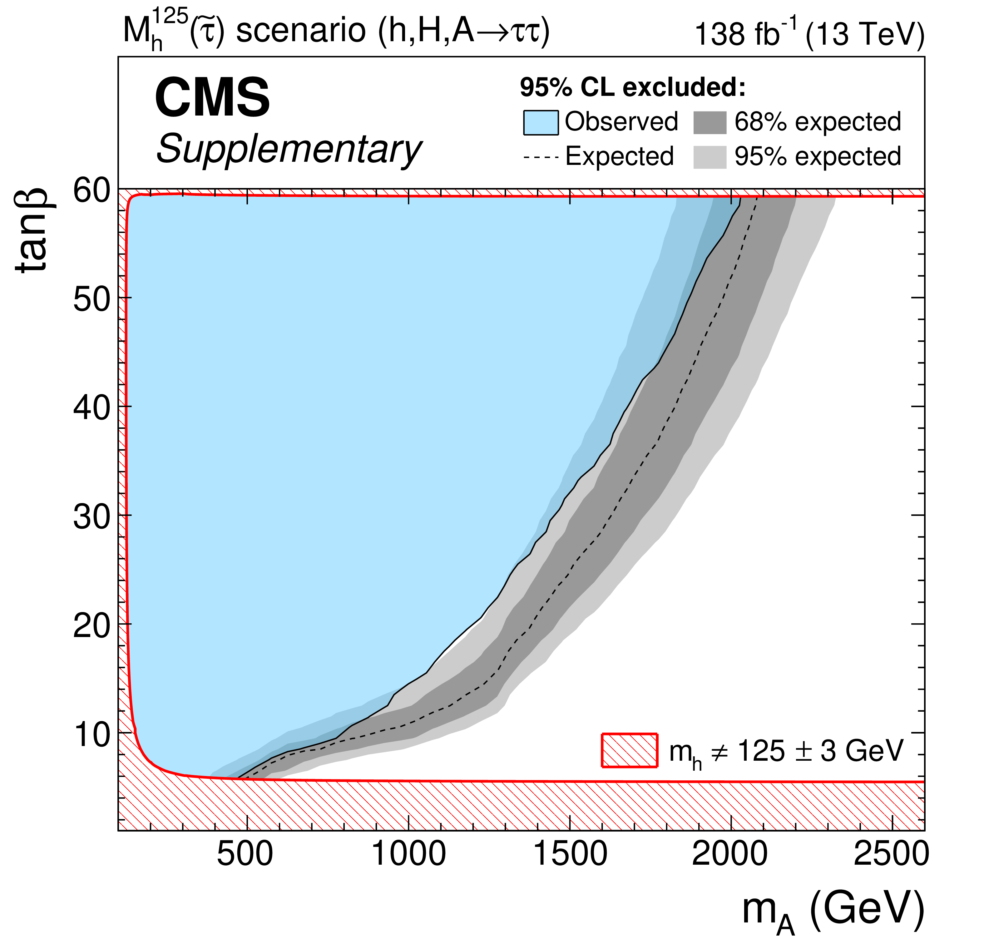
png pdf |
Additional Figure 114:
Expected and observed 95% CL exclusion contours in the MSSM $\mathrm{M_{h} }^{125}(\tilde{ \tau })$ scenario. The expected median in the absence of a signal is shown as a dashed black line. The dark and bright grey bands indicate the central 68% and 95% intervals of the expected exclusion. The observed exclusion contour is indicated by the coloured blue area. Those parts of the parameter space where $m_{\mathrm{h}}$ deviates by more than ${\pm}$3 GeV from the mass of H(125) are indicated by a red hatched area. |

png pdf |
Additional Figure 115:
Expected and observed 95% CL exclusion contours in the MSSM $\mathrm{M_{h} }^{125}(\tilde{\chi})$ scenario. The expected median in the absence of a signal is shown as a dashed black line. The dark and bright grey bands indicate the central 68% and 95% intervals of the expected exclusion. The observed exclusion contour is indicated by the coloured blue area. Those parts of the parameter space where $m_{\mathrm{h}}$ deviates by more than ${\pm}$3 GeV from the mass of H(125) are indicated by a red hatched area. |

png pdf |
Additional Figure 116:
Expected and observed 95% CL exclusion contours in the MSSM $\mathrm{M}_{\mathrm{h} }^{125\,\mu_{1}-}$ scenario. The expected median in the absence of a signal is shown as a dashed black line. The dark and bright grey bands indicate the central 68% and 95% intervals of the expected exclusion. The observed exclusion contour is indicated by the coloured blue area. Those parts of the parameter space where $m_{\mathrm{h}}$ deviates by more than ${\pm}$3 GeV from the mass of H(125) are indicated by a red hatched area. |
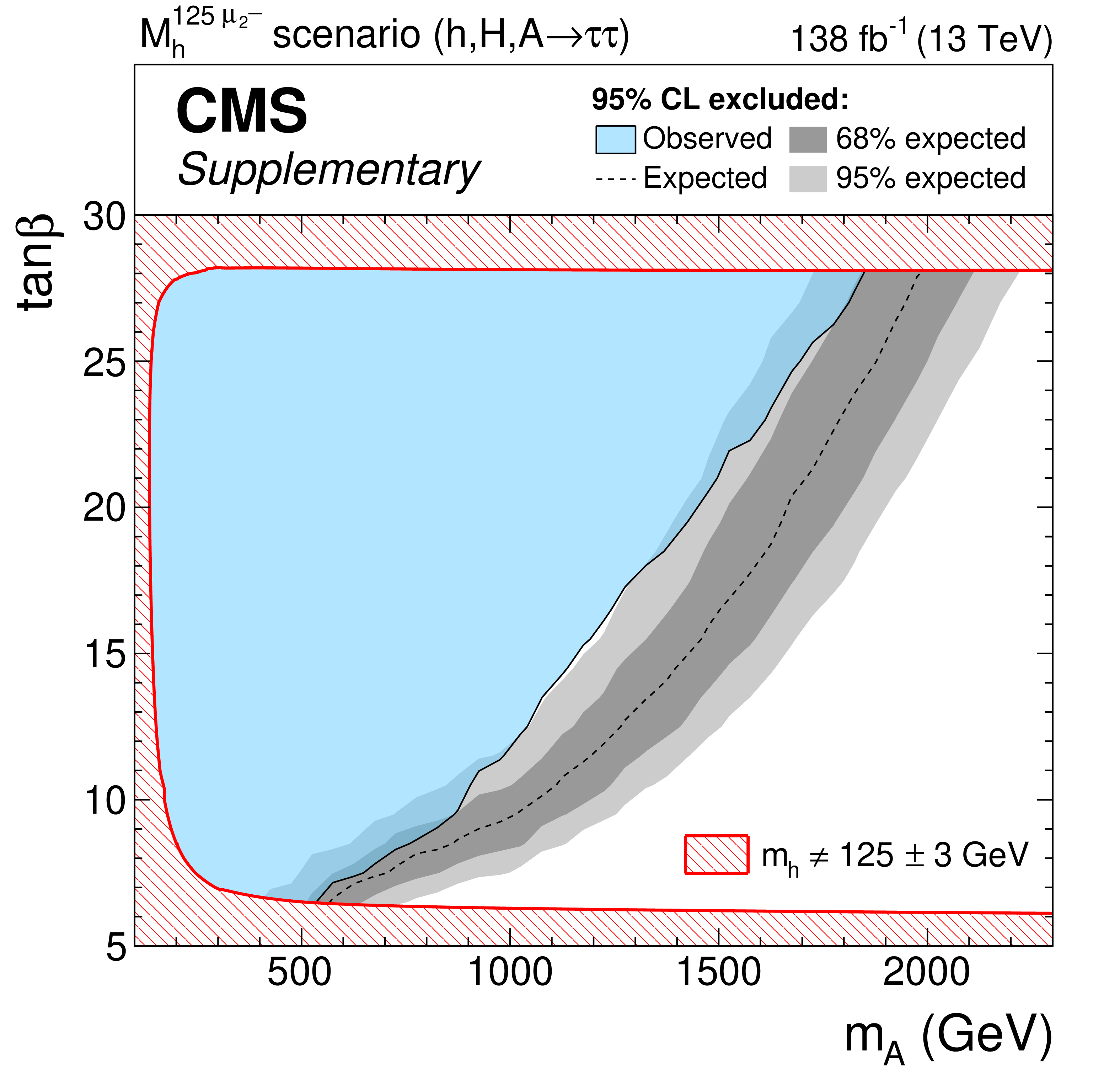
png pdf |
Additional Figure 117:
Expected and observed 95% CL exclusion contours in the MSSM $\mathrm{M}_{ \mathrm{h}}^{125\,\mu_{2}-}$ scenario. The expected median in the absence of a signal is shown as a dashed black line. The dark and bright grey bands indicate the central 68% and 95% intervals of the expected exclusion. The observed exclusion contour is indicated by the coloured blue area. Those parts of the parameter space where $m_{\mathrm{h}}$ deviates by more than ${\pm}$3 GeV from the mass of H(125) are indicated by a red hatched area. |
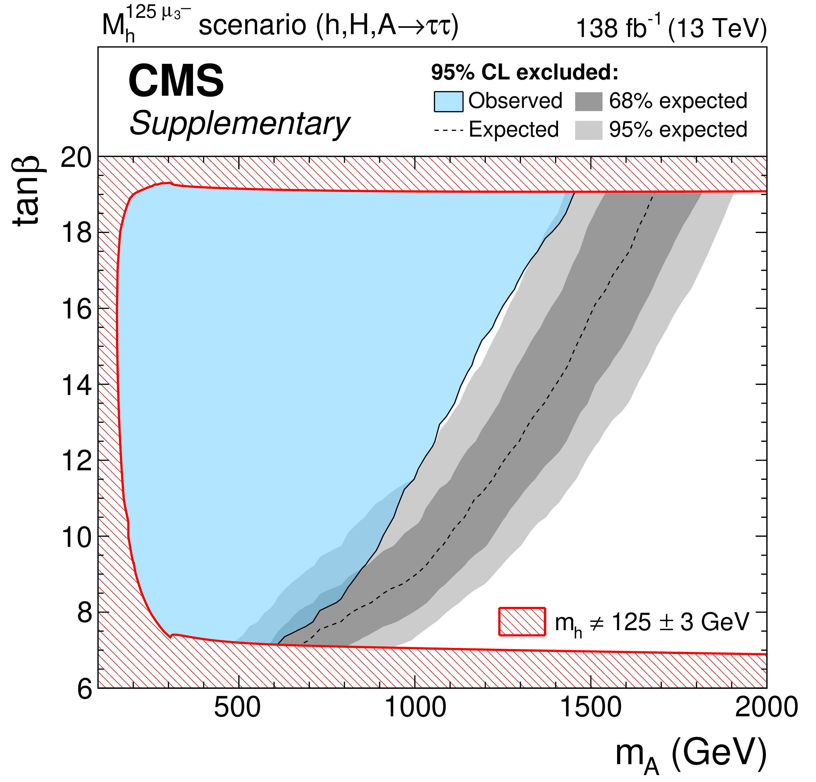
png pdf |
Additional Figure 118:
Expected and observed 95% CL exclusion contours in the MSSM $\mathrm{M}_{ \mathrm{h}}^{125\,\mu_{3}-}$ scenario. The expected median in the absence of a signal is shown as a dashed black line. The dark and bright grey bands indicate the central 68% and 95% intervals of the expected exclusion. The observed exclusion contour is indicated by the coloured blue area. Those parts of the parameter space where $m_{\mathrm{h}}$ deviates by more than ${\pm}$3 GeV from the mass of H(125) are indicated by a red hatched area. |
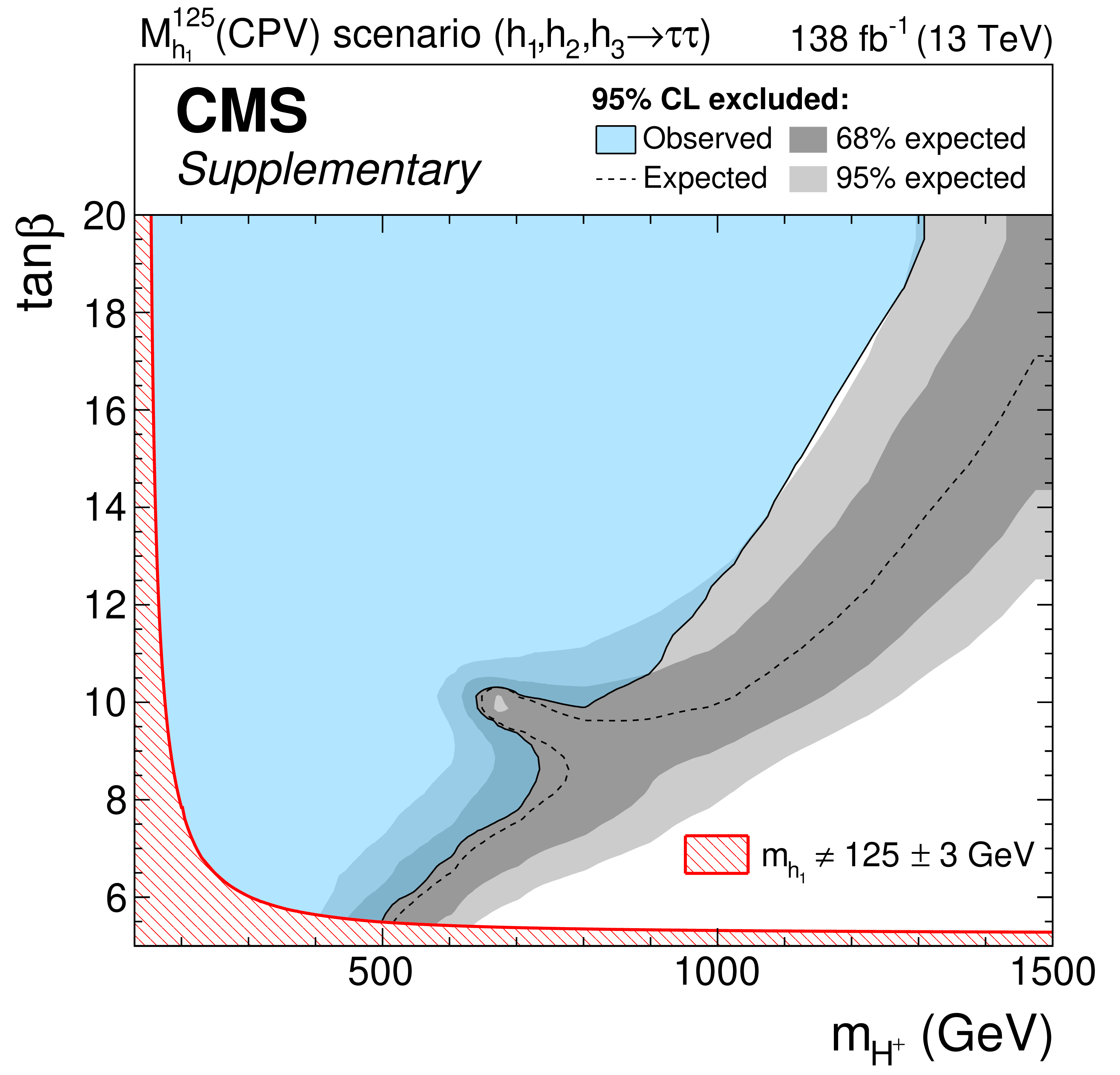
png pdf |
Additional Figure 119:
Expected and observed 95% CL exclusion contours in the MSSM $\mathrm{M_{h_{1} }^{125}(CPV)}$ scenario. The expected median in the absence of a signal is shown as a dashed black line. The dark and bright grey bands indicate the central 68% and 95% intervals of the expected exclusion. The observed exclusion contour is indicated by the coloured blue area. Those parts of the parameter space where $m_{\mathrm{h}_{1}}$ deviates by more than ${\pm}$3 GeV from the mass of H(125) are indicated by a red hatched area. |

png pdf |
Additional Figure 120:
Expected and observed 95% CL exclusion contours in the $\mathrm{hMSSM}$ scenario. The expected median in the absence of a signal is shown as a dashed black line. The dark and bright grey bands indicate the central 68% and 95% intervals of the expected exclusion. The observed exclusion contour is indicated by the coloured blue area. |
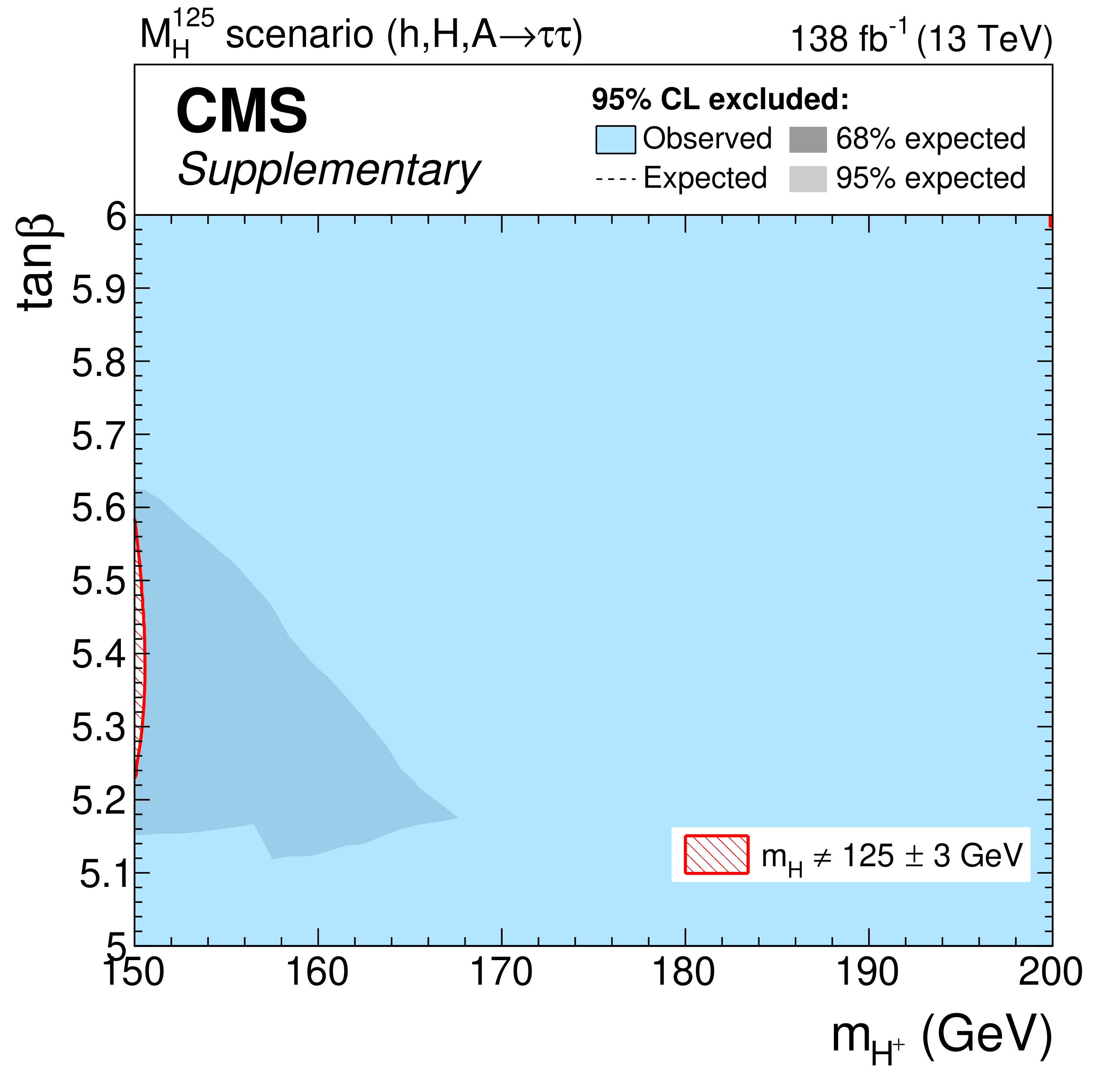
png pdf |
Additional Figure 121:
Expected and observed 95% CL exclusion contours in the MSSM $\mathrm{M}_{\mathrm{H}}^{125}$ scenario. The expected median in the absence of a signal is shown as a dashed black line. The dark and bright grey bands indicate the central 68% and 95% intervals of the expected exclusion. The observed exclusion contour is indicated by the coloured blue area. Those parts of the parameter space where $m_{\mathrm{H}}$ deviates by more than ${\pm}$3 GeV from the mass of H(125) are indicated by a red hatched area. |
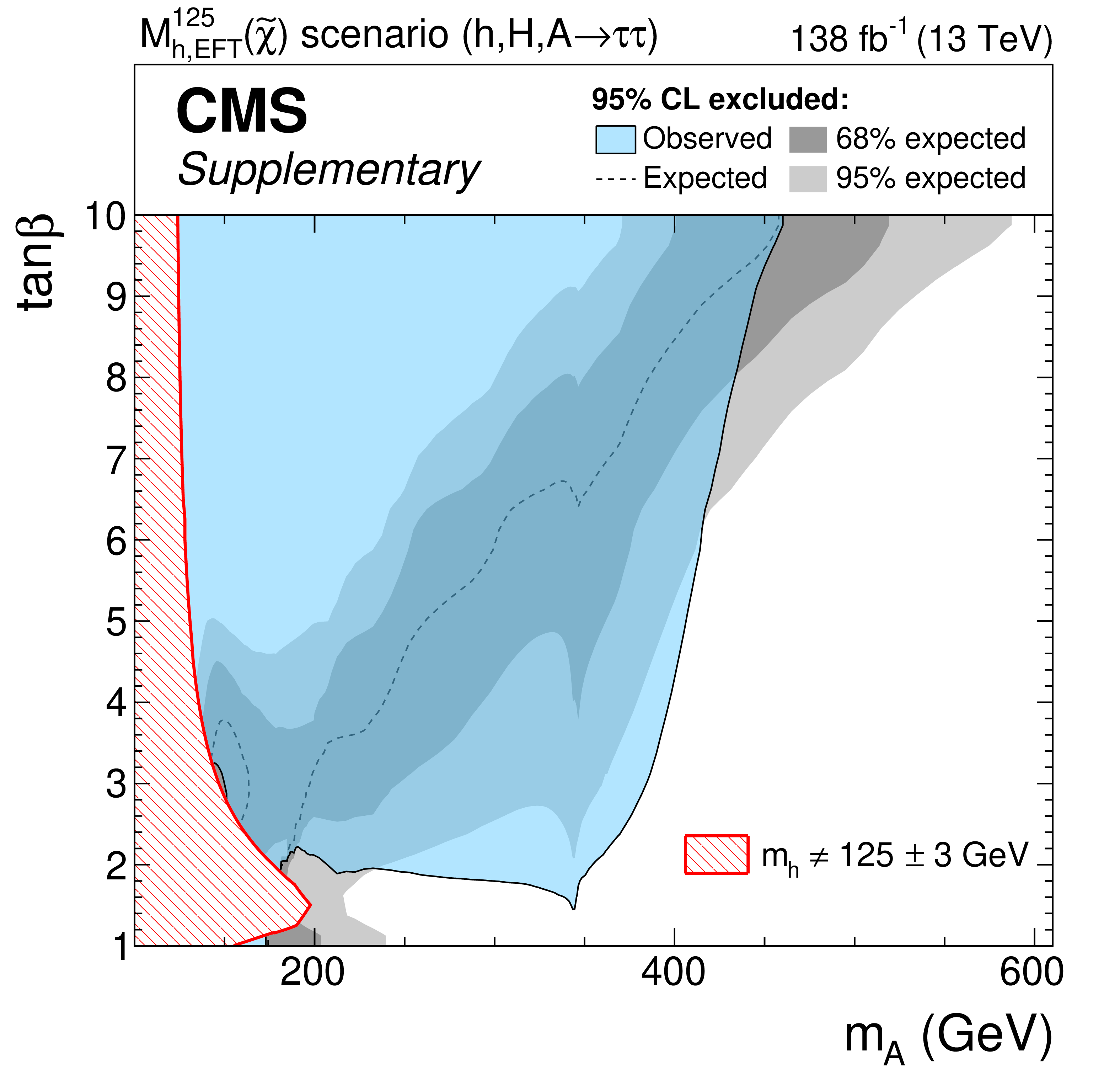
png pdf |
Additional Figure 122:
Expected and observed 95% CL exclusion contours in the MSSM $\mathrm{M_{h, \,EFT}^{125}}(\tilde{\chi})$ scenario. The expected median in the absence of a signal is shown as a dashed black line. The dark and bright grey bands indicate the central 68% and 95% intervals of the expected exclusion. The observed exclusion contour is indicated by the coloured blue area. Those parts of the parameter space where $m_{\mathrm{h}}$ deviates by more than ${\pm}$3 GeV from the mass of H(125) are indicated by a red hatched area. |
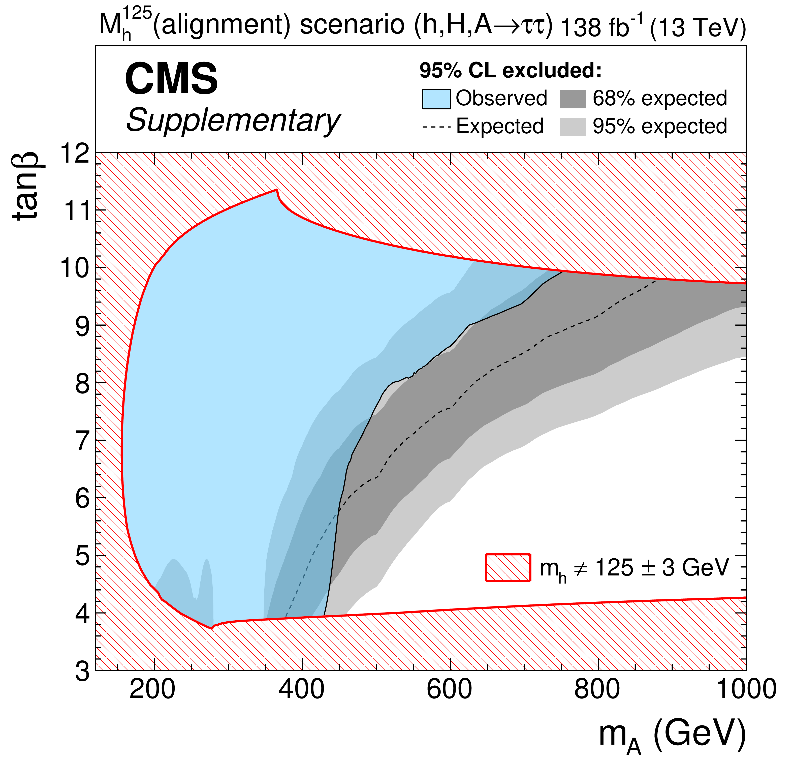
png pdf |
Additional Figure 123:
Expected and observed 95% CL exclusion contours in the $\mathrm{M}_{\mathrm{h}}^{125}$ (alignment) scenario. The expected median in the absence of a signal is shown as a dashed black line. The dark and bright grey bands indicate the central 68% and 95% intervals of the expected exclusion. The observed exclusion contour is indicated by the coloured blue area. Those parts of the parameter space where $m_{\mathrm{h}}$ deviates by more than ${\pm}$3 GeV from the mass of H(125) are indicated by a red hatched area. |
|
Further information about Additional Figures Additional Figs. 1—9 display the equivalent plots to Fig. 9 for the categories that are not displayed in the paper. In this case a signal-plus-background fit has been performed where the signal mass is fixed to 100 GeV. Additional Figs. 10—24 display the distributions for all categories used in the search for low-mass signals (mφ < 250 GeV) after performing a background-only fit to the data. These plots differ from Fig. 9 and Additional Figs. 1—9 which display the distributions after a signal-plus-background fit instead of the background-only. These background-only distributions are intended to be used for re-intpretations in different signal models. Additional Figs. 25—30 display the equivalent plots to Fig. 8 for the categories that are not displayed in the paper. In this case a background-only fit has been performed. Additional Figs. 31—36 display the local p-values for each tested mass point for different assumption about the production modes. Additional Figs. 37—40 display limits on the cross sections times branching ratios similar to Fig. 10 except different assumptions are made about the production modes. Additional Figs. 41—63 display the equivalent plots to Fig. 11 for the other mass points that are tested in the analysis but not displayed in the paper. Additional Fig. 64 displays a 2D maximum likelihood scan for a 95 GeV signal under the assumption that the signal is produced by vector boson fusion or gluon fusion. Additional Figs. 65—86 present the results of the low-mass analysis in terms of the effective coupling strengths to top and bottom quarks as an alternative to the cross section times branching fraction scans (e.g Fig. 11). The motivation for these scans is allow the results to be interpreted in models that predict sizeable contributions to the gluon fusion loop from both top and bottom quarks. As the kinematics, and therefore signal acceptance, depends strongly on the loop content, the limits derived for the top-only (Additional Fig. 39) and bottom-only (Additional Fig. 40) extremes might not apply in such scenarios and therefore it would be more appropriate to use these coupling scans to test such models. In order produce scans in terms of couplings it is necessary to have predictions for the cross sections for the b-associated and gluon fusion production processes. The b-associated cross sections including the interference with the gluon fusion process are determined by scaling the cross sections provided by the LHCXSWG (bbH cross sections) for a SM-like Higgs boson by the top and bottom Yukawa couplings. The b-associated cross section without interference is scaled by the bottom Yukawa coupling squared, while the interference contribution is scaled by the product of the top and bottom Yukawa couplings. The gluon fusion cross sections are estimated as follows. The cross sections for the top-only, bottom-only, and top-bottom-interference are estimated using POWHEG at NLO accuracy. The top-only cross section is scaled by the top Yukawa coupling squared, the bottom-only is scaled by the bottom Yukawa coupling squared, and the top-bottom-interference is scaled by the product of the top and bottom Yukawa couplings. The three components are then summed together and multiplied by k-factors that account for higher order corrections. For each mass point, the k-factor is defined as the ratio of the cross sections computed at N3LO by the LHCXSWG (N3LO cross sections) to the cross section computed at NLO by POWHEG assuming SM Yukawa couplings. Additional Figs. 87—91 display the results of the by-channel, by-era, and by-category compatibility checks for the 100 GeV and 1.2 TeV signal mass hypotheses. Additional Fig. 92 displays the limits set on an alternative vector leptoquark model. The model parameters are chosen to align with another CMS analysis (CMS-EXO-19-016) targeting the same signature to allow a direct comparison between the two analyses. Additional Figs. 93—98 display the expected limits broken down by channel, era, and category. The purpose of these plots are to show how the individual channels/eras/categories contribute to the overall sensitivity of the analysis. Additional Figs. 99—113 display scans of the likelihood function vs the effective coupling for the leptoquark interpretation of the data. There are several purposes for these plots, which includes: to provide the likelihood scans for the combined result to allow the results to be re-intpreted more easily, to show how the no b-tag and b-tag categories each contribute to the combined result, and to compare the results more easily with the CMS-EXO-19-016 analysis. Additional Fig. 114—123 display the limits in the mA-tanβ plane for alternative MSSM benchmark models that were considered in the analysis but not displayed in the paper. The plots are equivalent to Fig. 13 in the paper. |
| References | ||||
| 1 | ATLAS Collaboration | Observation of a new particle in the search for the standard model Higgs boson with the ATLAS detector at the LHC | PLB 716 (2012) 1 | 1207.7214 |
| 2 | CMS Collaboration | Observation of a new boson at a mass of 125 GeV with the CMS experiment at the LHC | PLB 716 (2012) 30 | CMS-HIG-12-028 1207.7235 |
| 3 | CMS Collaboration | Observation of a new boson with mass near 125 GeV in pp collisions at $ \sqrt{s} = $ 7 and 8 TeV | JHEP 06 (2013) 081 | CMS-HIG-12-036 1303.4571 |
| 4 | ATLAS and CMS Collaborations | Measurements of the Higgs boson production and decay rates and constraints on its couplings from a combined ATLAS and CMS analysis of the LHC pp collision data at $ \sqrt{s}= $ 7 and 8 TeV | JHEP 08 (2016) 045 | 1606.02266 |
| 5 | CMS Collaboration | Combined measurements of Higgs boson couplings in proton-proton collisions at $ \sqrt{s}=$ 13 TeV | EPJC 79 (2019) 421 | CMS-HIG-17-031 1809.10733 |
| 6 | ATLAS Collaboration | Combined measurements of Higgs boson production and decay using up to 80 fb$ ^{-1} $ of proton-proton collision data at $ \sqrt{s}= $ 13 TeV collected with the ATLAS experiment | PRD 101 (2020) 012002 | 1909.02845 |
| 7 | CMS Collaboration | Measurements of the Higgs boson width and anomalous HVV couplings from on-shell and off-shell production in the four-lepton final state | PRD 99 (2019) 112003 | CMS-HIG-18-002 1901.00174 |
| 8 | CMS Collaboration | A measurement of the Higgs boson mass in the diphoton decay channel | PLB 805 (2020) 135425 | CMS-HIG-19-004 2002.06398 |
| 9 | Yu. A. Golfand and E. P. Likhtman | Extension of the algebra of Poincaré group generators and violation of p invariance | JEPTL 13 (1971)323 | |
| 10 | J. Wess and B. Zumino | Supergauge transformations in four dimensions | NPB 70 (1974) 39 | |
| 11 | P. Fayet | Supergauge invariant extension of the Higgs mechanism and a model for the electron and its neutrino | NPB 90 (1975) 104 | |
| 12 | P. Fayet | Spontaneously broken supersymmetric theories of weak, electromagnetic and strong interactions | PLB 69 (1977) 489 | |
| 13 | DELPHI, OPAL, ALEPH, L3 and LEP Working Group for Higgs Boson Searches Collaboration | Search for neutral MSSM Higgs bosons at LEP | EPJC 47 (2006) 547 | hep-ex/0602042 |
| 14 | CDF Collaboration | Search for Higgs bosons predicted in Two-Higgs-Doublet models via decays to tau lepton pairs in 1.96 TeV $ {\mathrm{p}}\bar{{\mathrm{p}}} $ collisions | PRL 103 (2009) 201801 | 0906.1014 |
| 15 | D0 Collaboration | Search for neutral Higgs bosons in the multi-b-jet topology in 5.2 fb$^{-1}$ of $ {\mathrm{p}}\bar{{\mathrm{p}}} $ collisions at $ \sqrt{s} = $ 1.96 TeV | PLB 698 (2011) 97 | 1011.1931 |
| 16 | D0 Collaboration | Search for Higgs bosons decaying to $ \tau^{+}\tau^{-} $ pairs in $ {\mathrm{p}}\bar{{\mathrm{p}}} $ collisions at $ \sqrt{s} = $ 1.96 TeV | PLB 707 (2012) 323 | 1106.4555 |
| 17 | CDF Collaboration | Search for Higgs bosons produced in association with b-quarks | PRD 85 (2012) 032005 | 1106.4782 |
| 18 | CMS Collaboration | Search for a Higgs boson decaying into a b-quark pair and produced in association with b quarks in proton-proton collisions at 7 TeV | PLB 722 (2013) 207 | CMS-HIG-12-033 1302.2892 |
| 19 | CMS Collaboration | Search for neutral MSSM Higgs bosons decaying into a pair of bottom quarks | JHEP 11 (2015) 071 | CMS-HIG-14-017 1506.08329 |
| 20 | CMS Collaboration | Search for beyond the standard model Higgs bosons decaying into a $ \mathrm{b\overline{b}} $ pair in pp collisions at $ \sqrt{s} = $ 13 TeV | JHEP 08 (2018) 113 | CMS-HIG-16-018 1805.12191 |
| 21 | ATLAS Collaboration | Search for heavy neutral Higgs bosons produced in association with b-quarks and decaying into b-quarks at $ \sqrt{s}= $ 13 TeV with the ATLAS detector | PRD 102 (2020) 032004 | 1907.02749 |
| 22 | ATLAS Collaboration | Search for the neutral Higgs bosons of the minimal supersymmetric standard model in pp collisions at $ \sqrt{s} = $ 7 TeV with the ATLAS detector | JHEP 02 (2013) 095 | 1211.6956 |
| 23 | CMS Collaboration | Search for neutral MSSM Higgs bosons decaying to $ \mu^{+} \mu^{-} $ in pp collisions at $ \sqrt{s} = $ 7 and 8 TeV | PLB 752 (2016) 221 | CMS-HIG-13-024 1508.01437 |
| 24 | CMS Collaboration | Search for MSSM higgs bosons decaying to $ \mu^{+}\mu^{-} $ in proton-proton collisions at $ \sqrt{s} = $ 13 TeV | PLB 798 (2019) 134992 | CMS-HIG-18-010 1907.03152 |
| 25 | ATLAS Collaboration | Search for scalar resonances decaying into $ \mu^{+}\mu^{-} $ in events with and without b-tagged jets produced in proton-proton collisions at $ \sqrt{s} = $ 13 TeV with the ATLAS detector | JHEP 07 (2019) 117 | 1901.08144 |
| 26 | ATLAS Collaboration | Search for neutral Higgs bosons of the minimal supersymmetric standard model in pp collisions at $ \sqrt{s} = $ 8 TeV with the ATLAS detector | JHEP 11 (2014) 056 | 1409.6064 |
| 27 | ATLAS Collaboration | Search for minimal supersymmetric standard model Higgs bosons H/A and for a Z' boson in the $ \tau \tau $ final state produced in pp collisions at $ \sqrt{s} = $ 13 TeV with the ATLAS detector | EPJC 76 (2016) 585 | 1608.00890 |
| 28 | ATLAS Collaboration | Search for additional heavy neutral Higgs and gauge bosons in the ditau final state produced in 36 fb$^{-1}$ of pp collisions at $ \sqrt{s} = $ 13 TeV with the ATLAS detector | JHEP 01 (2018) 055 | 1709.07242 |
| 29 | CMS Collaboration | Search for neutral minimal supersymmetric standard model Higgs bosons decaying to tau pairs in pp collisions at $ \sqrt{s} = $ 7 TeV | PRL 106 (2011) 231801 | CMS-HIG-10-002 1104.1619 |
| 30 | CMS Collaboration | Search for neutral Higgs bosons decaying to tau pairs in pp collisions at $ \sqrt{s} = $ 7 TeV | PLB 713 (2012) 68 | CMS-HIG-11-029 1202.4083 |
| 31 | CMS Collaboration | Search for neutral MSSM Higgs bosons decaying to a pair of tau leptons in pp collisions | JHEP 10 (2014) 160 | CMS-HIG-13-021 1408.3316 |
| 32 | CMS Collaboration | Search for additional neutral MSSM higgs bosons in the $ \tau\tau $ final state in proton-proton collisions at $ \sqrt{s}= $ 13 TeV | JHEP 09 (2018) 007 | CMS-HIG-17-020 1803.06553 |
| 33 | ATLAS Collaboration | Search for heavy Higgs bosons decaying into two tau leptons with the ATLAS detector using pp collisions at $ \sqrt{s}= $ 13 TeV | PRL 125 (2020) 051801 | 2002.12223 |
| 34 | J. Steggemann | Extended scalar sectors | Ann. Rev. Nucl. Part. Sci. 70 (2020) 197 | |
| 35 | B. Diaz, M. Schmaltz, and Y.-M. Zhong | The leptoquark hunter's guide: Pair production | JHEP 10 (2017) 097 | 1706.05033 |
| 36 | M. Schmaltz and Y.-M. Zhong | The leptoquark hunter's guide: Large coupling | JHEP 01 (2019) 132 | 1810.10017 |
| 37 | CMS Collaboration | Search for third-generation scalar leptoquarks and heavy right-handed neutrinos in final states with two tau leptons and two jets in proton-proton collisions at $ \sqrt{s}= $ 13 TeV | JHEP 07 (2017) 121 | CMS-EXO-16-023 1703.03995 |
| 38 | CMS Collaboration | Search for a singly produced third-generation scalar leptoquark decaying to a $ \tau $ lepton and a bottom quark in proton-proton collisions at $ \sqrt{s}= $ 13 TeV | JHEP 07 (2018) 115 | CMS-EXO-17-029 1806.03472 |
| 39 | CMS Collaboration | Search for heavy neutrinos and third-generation leptoquarks in hadronic states of two $ \tau $ leptons and two jets in proton-proton collisions at $ \sqrt{s}= $ 13 TeV | JHEP 03 (2019) 170 | CMS-EXO-17-016 1811.00806 |
| 40 | ATLAS Collaboration | Searches for third-generation scalar leptoquarks in $ \sqrt{s} = $ 13 TeV pp collisions with the ATLAS detector | JHEP 06 (2019) 144 | 1902.08103 |
| 41 | ATLAS Collaboration | Search for a scalar partner of the top quark in the all-hadronic $ \mathrm{t}\mathrm{\bar{t}} $ plus missing transverse momentum final state at $ \sqrt{s}= $ 13 TeV with the ATLAS detector | EPJC 80 (2020) 737 | 2004.14060 |
| 42 | CMS Collaboration | Search for singly and pair-produced leptoquarks coupling to third-generation fermions in proton-proton collisions at $ \sqrt{s} = $ 13 TeV | PLB 819 (2021) 136446 | CMS-EXO-19-015 2012.04178 |
| 43 | ATLAS Collaboration | Search for new phenomena in pp collisions in final states with tau leptons, b-jets, and missing transverse momentum with the ATLAS detector | PRD 104 (2021) 112005 | 2108.07665 |
| 44 | ATLAS Collaboration | Search for new phenomena in final states with b-jets and missing transverse momentum in $ \sqrt{s}= $ 13 TeV pp collisions with the ATLAS detector | JHEP 05 (2021) 093 | 2101.12527 |
| 45 | ATLAS Collaboration | Search for pair production of third-generation scalar leptoquarks decaying into a top quark and a $ \tau $-lepton in pp collisions at $ \sqrt{s} = $ 13 TeV with the ATLAS detector | JHEP 06 (2021) 179 | 2101.11582 |
| 46 | CMS Collaboration | HEPData record for this analysis | link | |
| 47 | W. Buchmuller, R. Ruckl, and D. Wyler | Leptoquarks in lepton - quark collisions | PLB 191 (1987) 442 | |
| 48 | J. C. Pati and A. Salam | Unified lepton-hadron symmetry and a gauge theory of the basic interactions | PRD 8 (1973) 1240 | |
| 49 | J. C. Pati and A. Salam | Lepton number as the fourth color | PRD 10 (1974) 275 | |
| 50 | H. Georgi and S. L. Glashow | Unity of all elementary particle forces | PRL 32 (1974) 438 | |
| 51 | H. Fritzsch and P. Minkowski | Unified interactions of leptons and hadrons | Ann. Phys. 93 (1975) 193 | |
| 52 | S. Dimopoulos and L. Susskind | Mass without scalars | NPB 155 (1979) 237 | |
| 53 | S. Dimopoulos | Technicolored signatures | NPB 168 (1980) 69 | |
| 54 | E. Farhi and L. Susskind | Technicolor | PR 74 (1981) 277 | |
| 55 | K. D. Lane and M. V. Ramana | Walking technicolor signatures at hadron colliders | PRD 44 (1991) 2678 | |
| 56 | B. Schrempp and F. Schrempp | Light leptoquarks | PLB 153 (1985) 101 | |
| 57 | B. Gripaios | Composite leptoquarks at the LHC | JHEP 02 (2010) 045 | 0910.1789 |
| 58 | G. R. Farrar and P. Fayet | Phenomenology of the production, decay, and detection of new hadronic states associated with supersymmetry | PLB 76 (1978) 575 | |
| 59 | P. Ramond | Dual theory for free fermions | PRD 3 (1971) 2415 | |
| 60 | A. Neveu and J. H. Schwarz | Factorizable dual model of pions | NPB 31 (1971) 86 | |
| 61 | D. V. Volkov and V. P. Akulov | Possible universal neutrino interaction | JEPTL 16 (1972)438 | |
| 62 | J. Wess and B. Zumino | A Lagrangian model invariant under supergauge transformations | PLB 49 (1974) 52 | |
| 63 | H. P. Nilles | Supersymmetry, supergravity and particle physics | PR 110 (1984) 1 | |
| 64 | R. Barbier et al. | R-parity violating supersymmetry | PR 420 (2005) 1 | hep-ph/0406039 |
| 65 | M. Tanaka and R. Watanabe | New physics in the weak interaction of $ \bar B\to D^{(*)}\tau\bar\nu $ | PRD 87 (2013) 034028 | 1212.1878 |
| 66 | R. Barbieri, G. Isidori, A. Pattori, and F. Senia | Anomalies in B-decays and U(2) flavour symmetry | EPJC 76 (2016) 67 | 1512.01560 |
| 67 | D. A. Faroughy, A. Greljo, and J. F. Kamenik | Confronting lepton flavor universality violation in B decays with high-$ {p_{\mathrm{T}}} $ tau lepton searches at LHC | PLB 764 (2017) 126 | 1609.07138 |
| 68 | M. Bordone, C. Cornella, J. Fuentes-Martin, and G. Isidori | A three-site gauge model for flavor hierarchies and flavor anomalies | PLB 779 (2018) 317 | 1712.01368 |
| 69 | L. Di Luzio, A. Greljo, and M. Nardecchia | Gauge leptoquark as the origin of B-physics anomalies | PRD 96 (2017) 115011 | 1708.08450 |
| 70 | A. Greljo and B. A. Stefanek | Third family quark-lepton unification at the TeV scale | PLB 782 (2018) 131 | 1802.04274 |
| 71 | A. Angelescu et al. | Single leptoquark solutions to the B-physics anomalies | PRD 104 (2021) 055017 | 2103.12504 |
| 72 | C. Cornella et al. | Reading the footprints of the B-meson flavor anomalies | JHEP 08 (2021) 050 | 2103.16558 |
| 73 | LHCb Collaboration | Test of lepton universality in beauty-quark decays | NP 18 (2022) 277 | 2103.11769 |
| 74 | BaBar Collaboration | Evidence for an excess of $ \bar{\mathrm{B}} \to \mathrm{D}^{(*)} \tau^-\bar{\nu}_\tau $ decays | PRL 109 (2012) 101802 | 1205.5442 |
| 75 | BaBar Collaboration | Measurement of an excess of $ \bar{\mathrm{B}} \to \mathrm{D}^{(*)}\tau^- \bar{\nu}_\tau $ decays and implications for charged higgs bosons | PRD 88 (2013) 072012 | 1303.0571 |
| 76 | Belle Collaboration | Measurement of the branching ratio of $ \bar{\mathrm{B}} \to \mathrm{D}^{(\ast)} \tau^- \bar{\nu}_\tau $ relative to $ \bar{\mathrm{B}} \to \mathrm{D}^{(\ast)} \ell^- \bar{\nu}_\ell $ decays with hadronic tagging at Belle | PRD 92 (2015) 072014 | 1507.03233 |
| 77 | LHCb Collaboration | Measurement of the ratio of branching fractions $ \mathcal{B}(\bar{\mathrm{B}}^0 \to \mathrm{D}^{*+}\tau^{-}\bar{\nu}_{\tau})/\mathcal{B}(\bar{\mathrm{B}}^0 \to \mathrm{D}^{*+}\mu^{-}\bar{\nu}_{\mu}) $ | PRL 115 (2015) 111803 | 1506.08614 |
| 78 | Belle Collaboration | Measurement of the $ \tau $ lepton polarization and $ R(\mathrm{D}^*) $ in the decay $ \bar{\mathrm{B}} \to \mathrm{D}^* \tau^- \bar{\nu}_\tau $ | PRL 118 (2017) 211801 | 1612.00529 |
| 79 | LHCb Collaboration | Test of lepton flavor universality by the measurement of the $ \mathrm{B}^0 \to \mathrm{D}^{*-} \tau^+ \nu_{\tau} $ branching fraction using three-prong $ \tau $ decays | PRD 97 (2018) 072013 | 1711.02505 |
| 80 | LHCb Collaboration | Measurement of the ratio of the $ \mathrm{B}^0 \to \mathrm{D}^{*-} \tau^+ \nu_{\tau} $ and $ \mathrm{B}^0 \to \mathrm{D}^{*-} \mu^+ \nu_{\mu} $ branching fractions using three-prong $ \tau $-lepton decays | PRL 120 (2018) 171802 | 1708.08856 |
| 81 | T. D. Lee | A theory of spontaneous T violation | PRD 8 (1973) 1226 | |
| 82 | G. C. Branco et al. | Theory and phenomenology of two-Higgs-doublet models | PR 516 (2012) 1 | 1106.0034 |
| 83 | E. Bagnaschi et al. | MSSM Higgs boson searches at the LHC: Benchmark scenarios for Run 2 and beyond | EPJC 79 (2019) 617 | 1808.07542 |
| 84 | H. Bahl et al. | HL-LHC and ILC sensitivities in the hunt for heavy Higgs bosons | EPJC 80 (2020) 916 | 2005.14536 |
| 85 | H. Bahl, S. Liebler, and T. Stefaniak | MSSM Higgs benchmark scenarios for Run 2 and beyond: the low $ \tan\beta $ region | EPJC 79 (2019) 279 | 1901.05933 |
| 86 | E. A. Bagnaschi et al. | Benchmark scenarios for MSSM Higgs boson searches at the LHC | LHCHWG-2021-001, CERN | |
| 87 | LHC Higgs Cross Section Working Group -- MSSM subgroup | LHCHWG MSSM ROOT files | 2022 | |
| 88 | CMS Collaboration | Performance of the CMS Level-1 trigger in proton-proton collisions at $ \sqrt{s} = $ 13 TeV | JINST 15 (2020) P10017 | CMS-TRG-17-001 2006.10165 |
| 89 | CMS Collaboration | The CMS trigger system | JINST 12 (2017) P01020 | CMS-TRG-12-001 1609.02366 |
| 90 | CMS Collaboration | The CMS experiment at the CERN LHC | JINST 3 (2008) S08004 | CMS-00-001 |
| 91 | CMS Collaboration | Particle-flow reconstruction and global event description with the CMS detector | JINST 12 (2017) P10003 | CMS-PRF-14-001 1706.04965 |
| 92 | CMS Collaboration | Technical proposal for the Phase-II upgrade of the Compact Muon Solenoid | CMS-PAS-TDR-15-002 | CMS-PAS-TDR-15-002 |
| 93 | CMS Collaboration | Performance of electron reconstruction and selection with the CMS detector in proton-proton collisions at $ \sqrt{s} = $ 8 TeV | JINST 10 (2015) P06005 | CMS-EGM-13-001 1502.02701 |
| 94 | CMS Collaboration | Electron and photon reconstruction and identification with the CMS experiment at the CERN LHC | JINST 16 (2021) P05014 | CMS-EGM-17-001 2012.06888 |
| 95 | CMS Collaboration | Performance of the CMS muon detector and muon reconstruction with proton-proton collisions at $ \sqrt{s}= $ 13 TeV | JINST 13 (2018) P06015 | CMS-MUO-16-001 1804.04528 |
| 96 | M. Cacciari, G. P. Salam, and G. Soyez | The anti-$ {k_{\mathrm{T}}} $ jet clustering algorithm | JHEP 04 (2008) 063 | 0802.1189 |
| 97 | M. Cacciari, G. P. Salam, and G. Soyez | FastJet user manual | EPJC 72 (2012) 1896 | 1111.6097 |
| 98 | CMS Collaboration | Identification of heavy-flavour jets with the CMS detector in pp collisions at 13 TeV | JINST 13 (2018) P05011 | CMS-BTV-16-002 1712.07158 |
| 99 | E. Bols et al. | Jet flavour classification using DeepJet | JINST 15 (2020) P12012 | 2008.10519 |
| 100 | CMS Collaboration | Performance of the DeepJet b tagging algorithm using 41.9/fb of data from proton-proton collisions at 13 TeV with Phase 1 CMS detector | CDS | |
| 101 | CMS Collaboration | Performance of reconstruction and identification of $ \tau $ leptons decaying to hadrons and $ \nu_\tau $ in pp collisions at $ \sqrt{s}= $ 13 TeV | JINST 13 (2018) P10005 | CMS-TAU-16-003 1809.02816 |
| 102 | CMS Collaboration | Identification of hadronic tau lepton decays using a deep neural network | JINST 17 (2022) P07023 | CMS-TAU-20-001 2201.08458 |
| 103 | CMS Collaboration | Performance of missing transverse momentum reconstruction in proton-proton collisions at $ \sqrt{s} = $ 13 TeV using the CMS detector | JINST 14 (2019) P07004 | CMS-JME-17-001 1903.06078 |
| 104 | D. Bertolini, P. Harris, M. Low, and N. Tran | Pileup per particle identification | JHEP 10 (2014) 059 | 1407.6013 |
| 105 | CDF Collaboration | Search for neutral Higgs bosons of the minimal supersymmetric standard model decaying to $ \tau $ pairs in $ {\mathrm{p}}\bar{{\mathrm{p}}} $ collisions at $ \sqrt{s} = $ 1.96 TeV | PRL 96 (2006) 011802 | hep-ex/0508051 |
| 106 | L. Bianchini, J. Conway, E. K. Friis, and C. Veelken | Reconstruction of the Higgs mass in H $\to\tau\tau $ events by dynamical likelihood techniques | J. Phys. Conf. Ser. 513 (2014) 022035 | |
| 107 | B. K. Bullock, K. Hagiwara, and A. D. Martin | Tau polarization and its correlations as a probe of new physics | NPB 395 (1993) 499 | |
| 108 | Particle Data Group, P. A. Zyla et al. | Review of particle physics | Prog. Theor. Exp. Phys. 2020 (2020) 083C01 | |
| 109 | CMS Collaboration | Measurements of Higgs boson production in the decay channel with a pair of $ \tau $ leptons in proton-proton collisions at $ \sqrt{s} = $ 13 TeV | 2022. Submitted to EPJC | CMS-HIG-19-010 2204.12957 |
| 110 | CMS Collaboration | An embedding technique to determine $ \tau\tau $ backgrounds in proton-proton collision data | JINST 14 (2019) P06032 | CMS-TAU-18-001 1903.01216 |
| 111 | CMS Collaboration | Measurement of the $ \mathrm{Z}/\gamma^{*} \to \tau\tau $ cross section in pp collisions at $ \sqrt{s} = $ 13 TeV and validation of $ \tau $ lepton analysis techniques | EPJC 78 (2018) 708 | CMS-HIG-15-007 1801.03535 |
| 112 | J. Alwall et al. | MadGraph 5: Going beyond | JHEP 06 (2011) 128 | 1106.0522 |
| 113 | J. Alwall et al. | The automated computation of tree-level and next-to-leading order differential cross sections, and their matching to parton shower simulations | JHEP 07 (2014) 079 | 1405.0301 |
| 114 | R. Frederix and S. Frixione | Merging meets matching in MC@NLO | JHEP 12 (2012) 061 | 1209.6215 |
| 115 | J. Alwall et al. | Comparative study of various algorithms for the merging of parton showers and matrix elements in hadronic collisions | EPJC 53 (2008) 473 | 0706.2569 |
| 116 | S. Alioli, S.-O. Moch, and P. Uwer | Hadronic top-quark pair-production with one jet and parton showering | JHEP 01 (2012) 137 | 1110.5251 |
| 117 | R. Frederix, E. Re, and P. Torrielli | Single-top $ t $-channel hadroproduction in the four-flavour scheme with POWHEG and aMC@NLO | JHEP 09 (2012) 130 | 1207.5391 |
| 118 | P. Nason | A new method for combining NLO QCD with shower Monte Carlo algorithms | JHEP 11 (2004) 040 | hep-ph/0409146 |
| 119 | S. Frixione, P. Nason, and C. Oleari | Matching NLO QCD computations with parton shower simulations: the POWHEG method | JHEP 11 (2007) 070 | 0709.2092 |
| 120 | S. Alioli, P. Nason, C. Oleari, and E. Re | A general framework for implementing NLO calculations in shower Monte Carlo programs: the POWHEG BOX | JHEP 06 (2010) 043 | 1002.2581 |
| 121 | T. Je\vzo and P. Nason | On the treatment of resonances in next-to-leading order calculations matched to a parton shower | JHEP 12 (2015) 065 | 1509.09071 |
| 122 | E. Re | Single-top Wt-channel production matched with parton showers using the POWHEG method | EPJC 71 (2011) 1547 | 1009.2450 |
| 123 | K. Melnikov and F. Petriello | Electroweak gauge boson production at hadron colliders through $ \mathcal{O}(\alpha_\text{s}^{2}) $ | PRD 74 (2006) 114017 | hep-ph/0609070 |
| 124 | M. Czakon and A. Mitov | Top++: A program for the calculation of the top-pair cross-section at hadron colliders | CPC 185 (2014) 2930 | 1112.5675 |
| 125 | N. Kidonakis | Top quark production | in Helmholtz International Summer School on Physics of Heavy Quarks and Hadrons, 2014 | 1311.0283 |
| 126 | J. M. Campbell, R. K. Ellis, and C. Williams | Vector boson pair production at the LHC | JHEP 07 (2011) 018 | 1105.0020 |
| 127 | T. Gehrmann et al. | W$^{+}$W$^{-}$ production at hadron colliders in next to next to leading order QCD | PRL 113 (2014) 212001 | 1408.5243 |
| 128 | E. Bagnaschi, G. Degrassi, P. Slavich, and A. Vicini | Higgs production via gluon fusion in the POWHEG approach in the SM and in the MSSM | JHEP 02 (2012) 088 | 1111.2854 |
| 129 | P. Nason and C. Oleari | NLO Higgs boson production via vector-boson fusion matched with shower in POWHEG | JHEP 02 (2010) 037 | 0911.5299 |
| 130 | G. Luisoni, P. Nason, C. Oleari, and F. Tramontano | HW$^{\pm}$/HZ + 0 and 1 jet at NLO with the POWHEG BOX interfaced to GoSam and their merging within MiNLO | JHEP 10 (2013) 083 | 1306.2542 |
| 131 | F. Granata, J. M. Lindert, C. Oleari, and S. Pozzorini | NLO QCD+EW predictions for HV and HV+jet production including parton-shower effects | JHEP 09 (2017) 012 | 1706.03522 |
| 132 | K. Hamilton, P. Nason, E. Re, and G. Zanderighi | NNLOPS simulation of Higgs boson production | JHEP 10 (2013) 222 | 1309.0017 |
| 133 | K. Hamilton, P. Nason, and G. Zanderighi | Finite quark-mass effects in the NNLOPS POWHEG+MiNLO Higgs generator | JHEP 05 (2015) 140 | 1501.04637 |
| 134 | R. V. Harlander, H. Mantler, and M. Wiesemann | Transverse momentum resummation for Higgs production via gluon fusion in the MSSM | JHEP 11 (2014) 116 | 1409.0531 |
| 135 | E. Bagnaschi et al. | Resummation ambiguities in the Higgs transverse-momentum spectrum in the standard model and beyond | JHEP 01 (2016) 090 | 1510.08850 |
| 136 | E. Bagnaschi and A. Vicini | The Higgs transverse momentum distribution in gluon fusion as a multiscale problem | JHEP 01 (2016) 056 | 1505.00735 |
| 137 | B. Jager, L. Reina, and D. Wackeroth | Higgs boson production in association with b jets in the POWHEG BOX | PRD 93 (2016) 014030 | 1509.05843 |
| 138 | M. J. Baker, J. Fuentes-Mart\'in, G. Isidori, and M. Konig | High- $ {p_{\mathrm{T}}} $ signatures in vector-leptoquark models | EPJC 79 (2019) 334 | 1901.10480 |
| 139 | J. Butterworth et al. | PDF4LHC recommendations for LHC Run II | JPG 43 (2016) 023001 | 1510.03865 |
| 140 | NNPDF Collaboration | Parton distributions from high-precision collider data | EPJC 77 (2017) 663 | 1706.00428 |
| 141 | NNPDF Collaboration | Parton distributions for the LHC Run II | JHEP 04 (2015) 040 | 1410.8849 |
| 142 | CMS Collaboration | Event generator tunes obtained from underlying event and multiparton scattering measurements | EPJC 76 (2016) 155 | CMS-GEN-14-001 1512.00815 |
| 143 | CMS Collaboration | Extraction and validation of a new set of CMS PYTHIA8 tunes from underlying-event measurements | EPJC 80 (2020) 4 | CMS-GEN-17-001 1903.12179 |
| 144 | T. Sjostrand et al. | An introduction to PYTHIA 8.2 | CPC 191 (2015) 159 | 1410.3012 |
| 145 | GEANT4 Collaboration | GEANT4--a simulation toolkit | NIMA 506 (2003) 250 | |
| 146 | CMS Collaboration | Measurements of inclusive W and Z cross sections in pp collisions at $ \sqrt{s} = $ 7 TeV | JHEP 01 (2011) 080 | CMS-EWK-10-002 1012.2466 |
| 147 | CMS Collaboration | Measurement of the differential cross section for top quark pair production in pp collisions at $ \sqrt{s} = $ 8 TeV | EPJC 75 (2015) 542 | CMS-TOP-12-028 1505.04480 |
| 148 | R. J. Barlow and C. Beeston | Fitting using finite Monte Carlo samples | CPC 77 (1993) 219 | |
| 149 | J. S. Conway | Incorporating nuisance parameters in likelihoods for multisource spectra | in PHYSTAT 2011, p. 115 2011 | 1103.0354 |
| 150 | CMS Collaboration | Precision luminosity measurement in proton-proton collisions at $ \sqrt{s} = $ 13 TeV in 2015 and 2016 at CMS | EPJC 81 (2021) 800 | CMS-LUM-17-003 2104.01927 |
| 151 | CMS Collaboration | CMS luminosity measurement for the 2017 data taking period at $ \sqrt{s} = $ 13 TeV | CMS-PAS-LUM-17-004 | CMS-PAS-LUM-17-004 |
| 152 | CMS Collaboration | CMS luminosity measurement for the 2018 data-taking period at $ \sqrt{s} = $ 13 TeV | CMS-PAS-LUM-18-002 | CMS-PAS-LUM-18-002 |
| 153 | LHC Higgs Cross Section Working Group | Handbook of LHC Higgs cross sections: 4. deciphering the nature of the Higgs sector | CERN-2017-002-M | 1610.07922 |
| 154 | S. Alioli, P. Nason, C. Oleari, and E. Re | NLO Higgs boson production via gluon fusion matched with shower in POWHEG | JHEP 04 (2009) 002 | 0812.0578 |
| 155 | H. B. Hartanto, B. Jager, L. Reina, and D. Wackeroth | Higgs boson production in association with top quarks in the POWHEG BOX | PRD 91 (2015) 094003 | 1501.04498 |
| 156 | ATLAS and CMS Collaborations | Procedure for the LHC Higgs boson search combination in summer 2011 | ATL-PHYS-PUB 2011-11, CMS NOTE 2011/005 | |
| 157 | CMS Collaboration | Combined results of searches for the standard model Higgs boson in pp collisions at $ \sqrt{s} = $ 7 TeV | PLB 710 (2012) 26 | CMS-HIG-11-032 1202.1488 |
| 158 | G. Cowan, K. Cranmer, E. Gross, and O. Vitells | Asymptotic formulae for likelihood-based tests of new physics | EPJC 71 (2011) 1554 | 1007.1727 |
| 159 | T. Junk | Confidence level computation for combining searches with small statistics | NIMA 434 (1999) 435 | hep-ex/9902006 |
| 160 | A. L. Read | Presentation of search results: The CL$ _{\text{s}} $ technique | JPG 28 (2002) 2693 | |
| 161 | CMS Collaboration | Search for a standard model-like Higgs boson in the mass range between 70 and 110 GeV in the diphoton final state in proton-proton collisions at $ \sqrt{s}= $ 8 and 13 TeV | PLB (2019) 320 | CMS-HIG-17-013 1811.08459 |
| 162 | P. Slavich et al. | Higgs-mass predictions in the MSSM and beyond | EPJC 81 (2021) 450 | 2012.15629 |
| 163 | A. L. Read | Linear interpolation of histograms | NIMA 425 (1999) 357 | |
| 164 | S. Heinemeyer, W. Hollik, and G. Weiglein | FeynHiggs: A program for the calculation of the masses of the neutral CP-even Higgs bosons in the MSSM | CPC 124 (2000) 76 | hep-ph/9812320 |
| 165 | S. Heinemeyer, W. Hollik, and G. Weiglein | The masses of the neutral CP-even Higgs bosons in the MSSM: Accurate analysis at the two-loop level | EPJC 9 (1999) 343 | hep-ph/9812472 |
| 166 | G. Degrassi et al. | Towards high-precision predictions for the MSSM Higgs sector | EPJC 28 (2003) 133 | hep-ph/0212020 |
| 167 | M. Frank et al. | The Higgs boson masses and mixings of the complex MSSM in the Feynman-diagrammatic approach | JHEP 02 (2007) 047 | hep-ph/0611326 |
| 168 | T. Hahn et al. | High-precision predictions for the light CP-even Higgs boson mass of the minimal supersymmetric standard model | PRL 112 (2014) 141801 | 1312.4937 |
| 169 | H. Bahl and W. Hollik | Precise prediction for the light MSSM Higgs boson mass combining effective field theory and fixed-order calculations | EPJC 76 (2016) 499 | 1608.01880 |
| 170 | H. Bahl, S. Heinemeyer, W. Hollik, and G. Weiglein | Reconciling EFT and hybrid calculations of the light MSSM Higgs-boson mass | EPJC 78 (2018) 57 | 1706.00346 |
| 171 | H. Bahl et al. | Precision calculations in the MSSM Higgs-boson sector with FeynHiggs 2.14 | CPC 249 (2020) 107099 | 1811.09073 |
| 172 | A. Djouadi, J. Kalinowski, and M. Spira | HDECAY: A program for Higgs boson decays in the standard model and its supersymmetric extension | CPC 108 (1998) 56 | hep-ph/9704448 |
| 173 | A. Djouadi, J. Kalinowski, M. Muehlleitner, and M. Spira | HDECAY: Twenty++ years after | CPC 238 (2019) 214 | 1801.09506 |
| 174 | LHC Higgs Cross Section Working Group | Handbook of LHC Higgs cross sections: 3. Higgs properties | CERN-2013-004 | 1307.1347 |
| 175 | A. Denner et al. | Standard model Higgs-boson branching ratios with uncertainties | EPJC 71 (2011) 1753 | 1107.5909 |
| 176 | R. V. Harlander, S. Liebler, and H. Mantler | SusHi: A program for the calculation of Higgs production in gluon fusion and bottom-quark annihilation in the standard model and the MSSM | CPC 184 (2013) 1605 | 1212.3249 |
| 177 | R. V. Harlander, S. Liebler, and H. Mantler | SusHi Bento: Beyond NNLO and the heavy-top limit | CPC 212 (2017) 239 | 1605.03190 |
| 178 | M. Spira, A. Djouadi, D. Graudenz, and P. M. Zerwas | Higgs boson production at the LHC | NPB 453 (1995) 17 | hep-ph/9504378 |
| 179 | R. Harlander and P. Kant | Higgs production and decay: analytic results at next-to-leading order QCD | JHEP 12 (2005) 015 | hep-ph/0509189 |
| 180 | R. V. Harlander and W. B. Kilgore | Next-to-next-to-leading order Higgs production at hadron colliders | PRL 88 (2002) 201801 | hep-ph/0201206 |
| 181 | C. Anastasiou and K. Melnikov | Higgs boson production at hadron colliders in NNLO QCD | NPB 646 (2002) 220 | hep-ph/0207004 |
| 182 | V. Ravindran, J. Smith, and W. L. van Neerven | NNLO corrections to the total cross-section for Higgs boson production in hadron-hadron collisions | NPB 665 (2003) 325 | hep-ph/0302135 |
| 183 | R. V. Harlander and W. B. Kilgore | Production of a pseudo-scalar Higgs boson at hadron colliders at next-to-next-to leading order | JHEP 10 (2002) 017 | hep-ph/0208096 |
| 184 | C. Anastasiou and K. Melnikov | Pseudoscalar Higgs boson production at hadron colliders in next-to-next-to-leading order QCD | PRD 67 (2003) 037501 | hep-ph/0208115 |
| 185 | C. Anastasiou et al. | Higgs boson gluon-fusion production beyond threshold in N$ ^{3} $LO QCD | JHEP 03 (2015) 091 | 1411.3584 |
| 186 | C. Anastasiou et al. | Soft expansion of double-real-virtual corrections to Higgs production at N$ ^{3} $LO | JHEP 08 (2015) 051 | 1505.04110 |
| 187 | C. Anastasiou et al. | High precision determination of the gluon fusion Higgs boson cross-section at the LHC | JHEP 05 (2016) 058 | 1602.00695 |
| 188 | U. Aglietti, R. Bonciani, G. Degrassi, and A. Vicini | Two-loop light fermion contribution to Higgs production and decays | PLB 595 (2004) 432 | hep-ph/0404071 |
| 189 | R. Bonciani, G. Degrassi, and A. Vicini | On the generalized harmonic polylogarithms of one complex variable | CPC 182 (2011) 1253 | 1007.1891 |
| 190 | G. Degrassi and P. Slavich | NLO QCD bottom corrections to Higgs boson production in the MSSM | JHEP 11 (2010) 044 | 1007.3465 |
| 191 | G. Degrassi, S. Di Vita, and P. Slavich | NLO QCD corrections to pseudoscalar Higgs production in the MSSM | JHEP 08 (2011) 128 | 1107.0914 |
| 192 | G. Degrassi, S. Di Vita, and P. Slavich | On the NLO QCD corrections to the production of the heaviest neutral Higgs scalar in the MSSM | EPJC 72 (2012) 2032 | 1204.1016 |
| 193 | L. Hofer, U. Nierste, and D. Scherer | Resummation of tan-beta-enhanced supersymmetric loop corrections beyond the decoupling limit | JHEP 10 (2009) 081 | 0907.5408 |
| 194 | M. Bonvini, A. S. Papanastasiou, and F. J. Tackmann | Resummation and matching of b-quark mass effects in $ \mathrm{b}\overline{\mathrm{b}}\mathrm{H} $ production | JHEP 11 (2015) 196 | 1508.03288 |
| 195 | M. Bonvini, A. S. Papanastasiou, and F. J. Tackmann | Matched predictions for the $ \mathrm{b}\overline{\mathrm{b}}\mathrm{H} $ cross section at the 13 TeV LHC | JHEP 10 (2016) 053 | 1605.01733 |
| 196 | S. Dittmaier, M. Kramer, and M. Spira | Higgs radiation off bottom quarks at the Fermilab TeVatron and the CERN LHC | PRD 70 (2004) 074010 | hep-ph/0309204 |
| 197 | S. Dawson, C. B. Jackson, L. Reina, and D. Wackeroth | Exclusive Higgs boson production with bottom quarks at hadron colliders | PRD 69 (2004) 074027 | hep-ph/0311067 |
| 198 | R. V. Harlander and W. B. Kilgore | Higgs boson production in bottom quark fusion at next-to-next-to leading order | PRD 68 (2003) 013001 | hep-ph/0304035 |
| 199 | C. Duhr, F. Dulat, and B. Mistlberger | Higgs boson production in bottom-quark fusion to third order in the strong coupling | PRL 125 (2020) 051804 | 1904.09990 |
| 200 | S. Forte, D. Napoletano, and M. Ubiali | Higgs production in bottom-quark fusion in a matched scheme | PLB 751 (2015) 331 | 1508.01529 |
| 201 | S. Forte, D. Napoletano, and M. Ubiali | Higgs production in bottom-quark fusion: matching beyond leading order | PLB 763 (2016) 190 | 1607.00389 |
|
|
Compact Muon Solenoid LHC, CERN |
|

|

|

|

|

|