

Compact Muon Solenoid
LHC, CERN
| CMS-HIG-19-010 ; CERN-EP-2022-027 | ||
| Measurements of Higgs boson production in the decay channel with a pair of $ \tau $ leptons in proton-proton collisions at $\sqrt{s}= $ 13 TeV | ||
| CMS Collaboration | ||
| 27 April 2022 | ||
| Eur. Phys. J. C 83 (2023) 562 | ||
| Abstract: Measurements of Higgs boson production, where the Higgs boson decays into a pair of $ \tau $ leptons, are presented, using a sample of proton-proton collisions collected with the CMS experiment at a center-of-mass energy of 13 TeV, corresponding to an integrated luminosity of 138 fb$^{-1}$. Three analyses are presented. Two are targeting Higgs boson production via gluon fusion and vector boson fusion: a neural network based analysis and an analysis based on an event categorization optimized on the ratio of signal over background events. These are complemented by an analysis targeting vector boson associated Higgs boson production. Results are presented in the form of signal strengths relative to the standard model predictions and products of cross sections and branching fraction to $ \tau $ leptons, in up to 16 different kinematic regions. For the simultaneous measurements of the neural network based analysis and the analysis targeting vector boson associated Higgs boson production signal strengths are found to be 0.82 $ \pm $ 0.11 for inclusive Higgs boson production, 0.67 $ \pm $ 0.19 (0.81 $ \pm $ 0.17) for the production mainly via gluon fusion (vector boson fusion), and 1.79 $ \pm $ 0.45 for vector boson associated Higgs boson production. | ||
| Links: e-print arXiv:2204.12957 [hep-ex] (PDF) ; CDS record ; inSPIRE record ; HepData record ; CADI line (restricted) ; | ||
| Figures & Tables | Summary | Additional Figures & Tables | References | CMS Publications |
|---|
| Figures | |

png pdf |
Figure 1:
Binning for ggH production in the reduced STXS stage-1.2 scheme as exploited by the analyses presented in this paper. The dark gray boxes indicate the STXS bins measured by the analyses. Depending on the analysis, a split is applied to the 0-jet bin, as is indicated by the dashed line. The boxes colored in light gray indicate a finer subdivision of the NN signal classes for $ N_{\text{jet}} \geq $ 2 used for the classification task, as explained in Section 7. Thresholds on $ p_{\mathrm{T}} ^{ \mathrm{H} } $ are given in GeV. |

png pdf |
Figure 2:
Binning for qqH production in the reduced STXS stage-1.2 scheme as exploited by the analyses presented in this paper. The gray boxes indicate the STXS bins measured by the analyses. Thresholds on $ p_{\mathrm{T}} ^{ \mathrm{H} } $ and $ m_{\mathrm{jj}} $ are given in GeV. |

png pdf |
Figure 3:
Binning for VH production in the reduced STXS stage-1.2 scheme as exploited by the analysis presented in this paper. The gray boxes indicate the STXS bins measured by the analysis. Thresholds on $ p_{\mathrm{T}} ^{ \mathrm{V} } $ are given in GeV. |

png pdf |
Figure 4:
Confusion matrices for the NN classification tasks used for the (upper) STXS stage-0/inclusive and (lower) STXS stage-1.2 cross section measurements described in Section 7. These confusion matrices have been evaluated on the full test data set, comprising all data-taking years in the $ \mu \tau _\mathrm{h} $ final state. They are normalized such that all entries in each column, corresponding to a given true event class, sum to unity. |

png pdf |
Figure 4-a:
Confusion matrix for the NN classification tasks used for the STXS stage-0/inclusive cross section measurements described in Section 7. The matrix has been evaluated on the full test data set, comprising all data-taking years in the $ \mu \tau _\mathrm{h} $ final state. It is normalized such that all entries in each column, corresponding to a given true event class, sum to unity. |

png pdf |
Figure 4-b:
Confusion matrix for the NN classification tasks used for the STXS stage-1.2 cross section measurements described in Section 7. The matrix has been evaluated on the full test data set, comprising all data-taking years in the $ \mu \tau _\mathrm{h} $ final state. It is normalized such that all entries in each column, corresponding to a given true event class, sum to unity. |

png pdf |
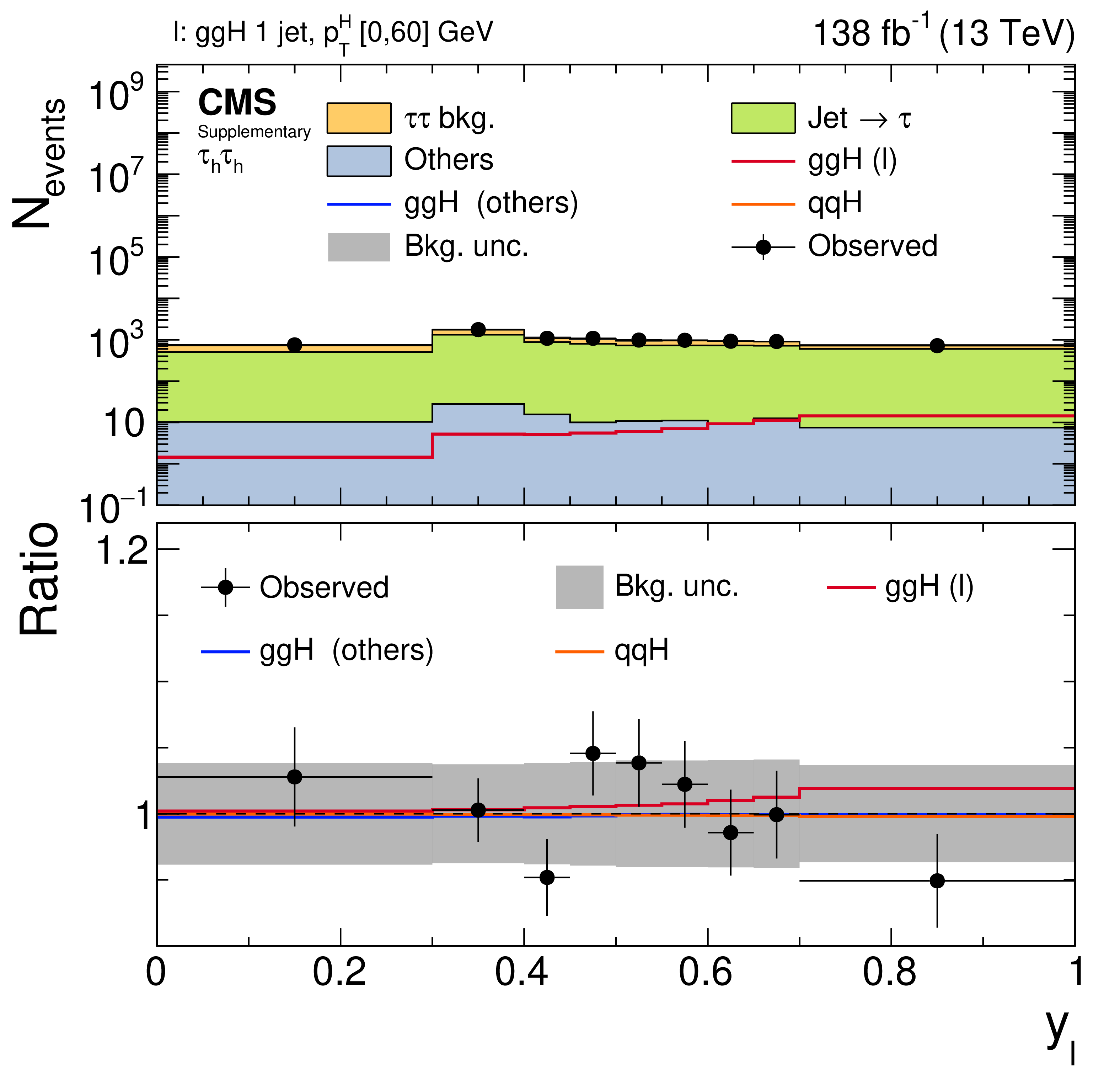
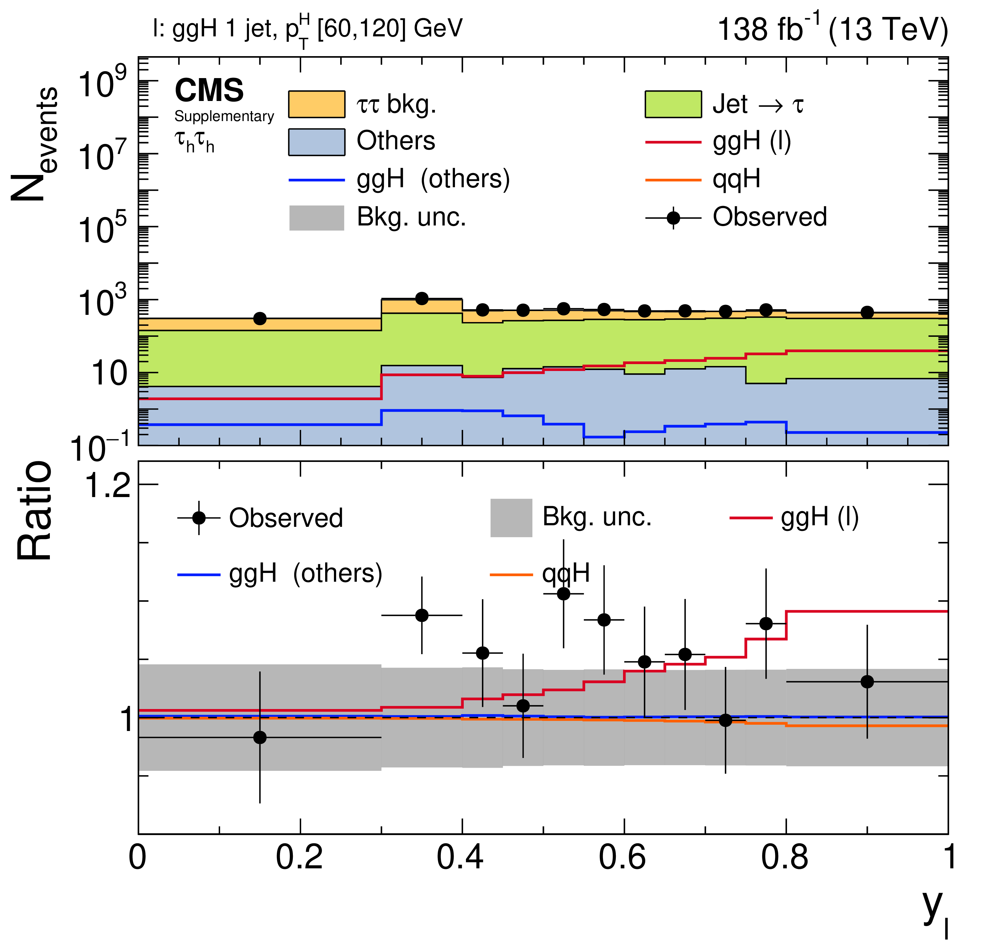
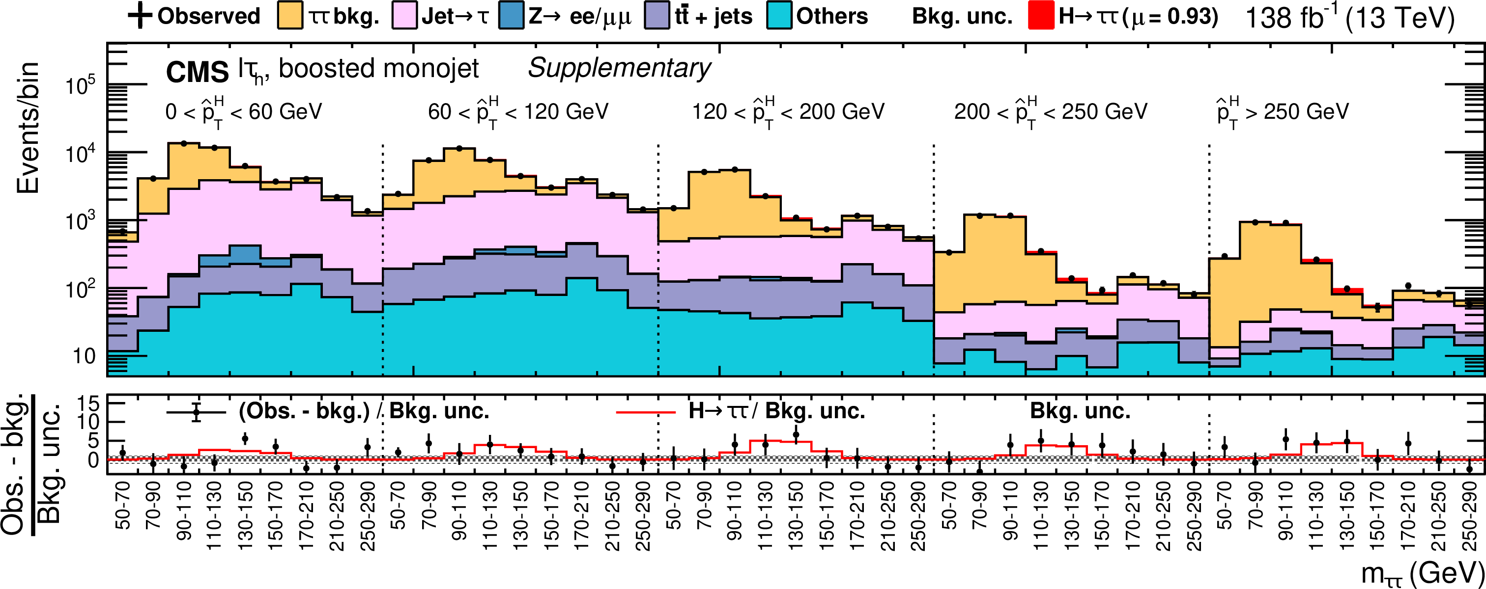
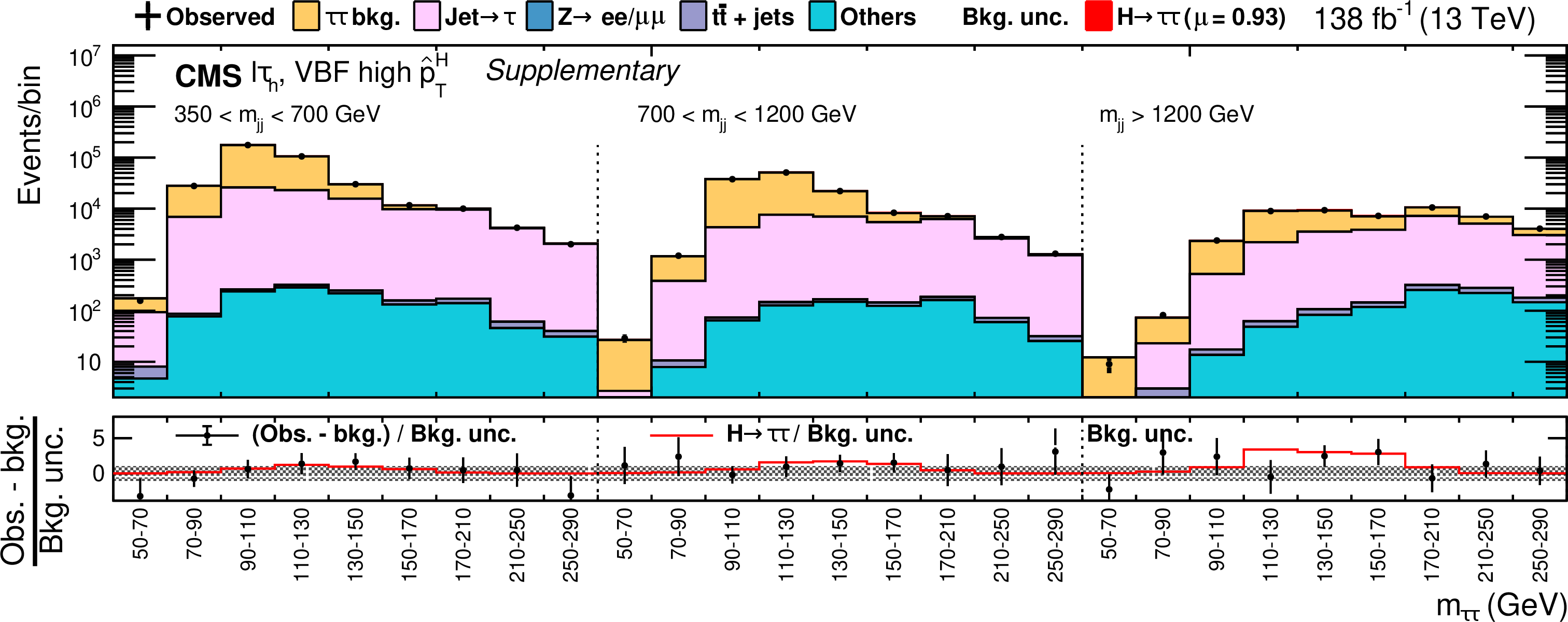
Figure 5:
Observed and predicted distributions of $ y_{l} $ for the signal classes for the ggH $ N_{\text{jet}} = $ 1 subspace in three increasing STXS stage-1.2 bins in $ p_{\mathrm{T}} ^{ \mathrm{H} } $ and the qqH $ N_{\text{jet}} \geq $ 2 bin with $ m_{\mathrm{jj}} \geq $ 700 GeV, $ p_{\mathrm{T}} ^{ \mathrm{H} } [0, 200] $ GeV, in the $ \mu \tau _\mathrm{h} $ final state of the NN-analysis. The distributions show all data-taking years combined. The signal contributions for (red) each STXS bin corresponding to the given event class, and the remaining inclusive (blue) ggH and (orange) qqH processes, excluding the STXS bin in consideration, are also shown as unstacked open histograms. All distributions are shown after the fit of the model, used for the extraction of the STXS stage-1.2 signals, to the data from all final states and data-taking years. Signal contributions in particular have been scaled according to the obtained fit results. In the lower panel of each plot the differences either of the corresponding additional signals or the data relative to the background expectation after fit are shown. |

png pdf |
Figure 5-a:
Observed and predicted distributions of $ y_{l} $ for the signal classes for the ggH $ N_{\text{jet}} = $ 1 subspace in STXS stage-1.2 bin in $ p_{\mathrm{T}} ^{ \mathrm{H} } [0,60] $ GeV, in the $ \mu \tau _\mathrm{h} $ final state of the NN-analysis. The distribution shows all data-taking years combined. The signal contributions for (red) each STXS bin corresponding to the given event class, and the remaining inclusive (blue) ggH and (orange) qqH processes, excluding the STXS bin in consideration, are also shown as unstacked open histograms. All distributions are shown after the fit of the model, used for the extraction of the STXS stage-1.2 signals, to the data from all final states and data-taking years. Signal contributions in particular have been scaled according to the obtained fit results. In the lower panel \the differences either of the corresponding additional signals or the data relative to the background expectation after fit are shown. |
png pdf |
Figure 5-b:
Observed and predicted distributions of $ y_{l} $ for the signal classes for the ggH $ N_{\text{jet}} = $ 1 subspace in STXS stage-1.2 bin in $ p_{\mathrm{T}} ^{ \mathrm{H} } [60,120] $ GeV, in the $ \mu \tau _\mathrm{h} $ final state of the NN-analysis. The distribution shows all data-taking years combined. The signal contributions for (red) each STXS bin corresponding to the given event class, and the remaining inclusive (blue) ggH and (orange) qqH processes, excluding the STXS bin in consideration, are also shown as unstacked open histograms. All distributions are shown after the fit of the model, used for the extraction of the STXS stage-1.2 signals, to the data from all final states and data-taking years. Signal contributions in particular have been scaled according to the obtained fit results. In the lower panel \the differences either of the corresponding additional signals or the data relative to the background expectation after fit are shown. |

png pdf |
Figure 5-c:
Observed and predicted distributions of $ y_{l} $ for the signal classes for the ggH $ N_{\text{jet}} = $ 1 subspace in STXS stage-1.2 bin in $ p_{\mathrm{T}} ^{ \mathrm{H} } [120,200] $ GeV, in the $ \mu \tau _\mathrm{h} $ final state of the NN-analysis. The distribution shows all data-taking years combined. The signal contributions for (red) each STXS bin corresponding to the given event class, and the remaining inclusive (blue) ggH and (orange) qqH processes, excluding the STXS bin in consideration, are also shown as unstacked open histograms. All distributions are shown after the fit of the model, used for the extraction of the STXS stage-1.2 signals, to the data from all final states and data-taking years. Signal contributions in particular have been scaled according to the obtained fit results. In the lower panel \the differences either of the corresponding additional signals or the data relative to the background expectation after fit are shown. |
png pdf |
Figure 5-d:
Observed and predicted distributions of $ y_{l} $ for the signal classes for the qqH $ N_{\text{jet}} \geq $ 2 bin with $ m_{\mathrm{jj}} \geq $ 700 GeV, $ p_{\mathrm{T}} ^{ \mathrm{H} } [0, 200] $ GeV, in the $ \mu \tau _\mathrm{h} $ final state of the NN-analysis. The distribution shows all data-taking years combined. The signal contributions for (red) each STXS bin corresponding to the given event class, and the remaining inclusive (blue) ggH and (orange) qqH processes, excluding the STXS bin in consideration, are also shown as unstacked open histograms. All distributions are shown after the fit of the model, used for the extraction of the STXS stage-1.2 signals, to the data from all final states and data-taking years. Signal contributions in particular have been scaled according to the obtained fit results. In the lower panel \the differences either of the corresponding additional signals or the data relative to the background expectation after fit are shown. |

png pdf |
Figure 6:
Observed and predicted distributions of the 2D discriminant as used for the extraction of the STXS stage-0 and inclusive signals, for all data-taking years in the $ \mu \tau _\mathrm{h} $ final state of the NN-analysis. Also shown is the definition of each individual bin, on the right. The background distributions are shown after the fit of the model, used for the extraction of the inclusive signal to the data from all final states and data-taking years. For this fit some of the bins have been merged to ensure a sufficient population of each bin. The distributions are shown with the finest common binning across all data-taking years. The signal contributions for the (red) inclusive, (blue) ggH, and (orange) qqH signals are also shown as unstacked open histograms, scaled according to the correspondingly obtained fit results. The vertical gray dashed lines indicate six primary bins in $ y_{ \mathrm{q} \mathrm{q} \mathrm{H} } $, the last four of which to the right have been enhanced by factors ranging from 3 to 15 for improved visibility. In the lower panel of the plot on the left the differences either of the corresponding additional signals or the data relative to the background expectation after fit are shown. |

png pdf |
Figure 6-a:
Observed and predicted distributions of the 2D discriminant as used for the extraction of the STXS stage-0 and inclusive signals, for all data-taking years in the $ \mu \tau _\mathrm{h} $ final state of the NN-analysis. The background distributions are shown after the fit of the model, used for the extraction of the inclusive signal to the data from all final states and data-taking years. For this fit some of the bins have been merged to ensure a sufficient population of each bin. The distributions are shown with the finest common binning across all data-taking years. The signal contributions for the (red) inclusive, (blue) ggH, and (orange) qqH signals are also shown as unstacked open histograms, scaled according to the correspondingly obtained fit results. The vertical gray dashed lines indicate six primary bins in $ y_{ \mathrm{q} \mathrm{q} \mathrm{H} } $, the last four of which to the right have been enhanced by factors ranging from 3 to 15 for improved visibility. In the lower panel of the plot the differences either of the corresponding additional signals or the data relative to the background expectation after fit are shown. |

png pdf |
Figure 6-b:
Shown is the definition of each individual bin. |

png pdf |
Figure 7:
Signal composition of the subcategories of the CB-analysis, in terms of the STXS stage-1.2 bins (in %). The rows correspond to the signal categories described in the text including the signal categories of the VH -analysis as described in Section 9. The columns refer to the STXS bins specified in Figs. 3--5. The STXS stage-1.2 qqH bin with $ N_{\text{jet}} < $ 2 or $ m_{\mathrm{jj}} < $ 350 GeV is labeled by ``qqH/non-VBF-topo''. This figure is based on all $ \tau \tau $ final states. |
png pdf |
Figure 8:
Observed and predicted 2D distributions in the ${\geq} $ 2 jet category of the (upper) $ \mathrm{e} \mu $, (middle) $ \ell \tau _\mathrm{h} $, and (lower) $ \tau _\mathrm{h} \tau _\mathrm{h} $ final states of the CB-analysis. The predicted signal and background distributions are shown after the fit used for the extraction of the inclusive signal. The ``Others'' background contribution includes events from diboson and single t quark production, as well as $ \mathrm{H} \to \mathrm{W} \mathrm{W} $ decays. The uncertainty bands account for all systematic and statistical sources of uncertainty, after the fit to the data. |

png pdf |
Figure 8-a:
Observed and predicted 2D distributions in the ${\geq} $ 2 jet category of the $ \mathrm{e} \mu $ final state of the CB-analysis. The predicted signal and background distributions are shown after the fit used for the extraction of the inclusive signal. The ``Others'' background contribution includes events from diboson and single t quark production, as well as $ \mathrm{H} \to \mathrm{W} \mathrm{W} $ decays. The uncertainty band accounts for all systematic and statistical sources of uncertainty, after the fit to the data. |

png pdf |
Figure 8-b:
Observed and predicted 2D distributions in the ${\geq} $ 2 jet category of the $ \ell \tau _\mathrm{h} $ final state of the CB-analysis. The predicted signal and background distributions are shown after the fit used for the extraction of the inclusive signal. The ``Others'' background contribution includes events from diboson and single t quark production, as well as $ \mathrm{H} \to \mathrm{W} \mathrm{W} $ decays. The uncertainty band accounts for all systematic and statistical sources of uncertainty, after the fit to the data. |
png pdf |
Figure 8-c:
Observed and predicted 2D distributions in the ${\geq} $ 2 jet category of the $ \tau _\mathrm{h} \tau _\mathrm{h} $ final state of the CB-analysis. The predicted signal and background distributions are shown after the fit used for the extraction of the inclusive signal. The ``Others'' background contribution includes events from diboson and single t quark production, as well as $ \mathrm{H} \to \mathrm{W} \mathrm{W} $ decays. The uncertainty band accounts for all systematic and statistical sources of uncertainty, after the fit to the data. |
png pdf |
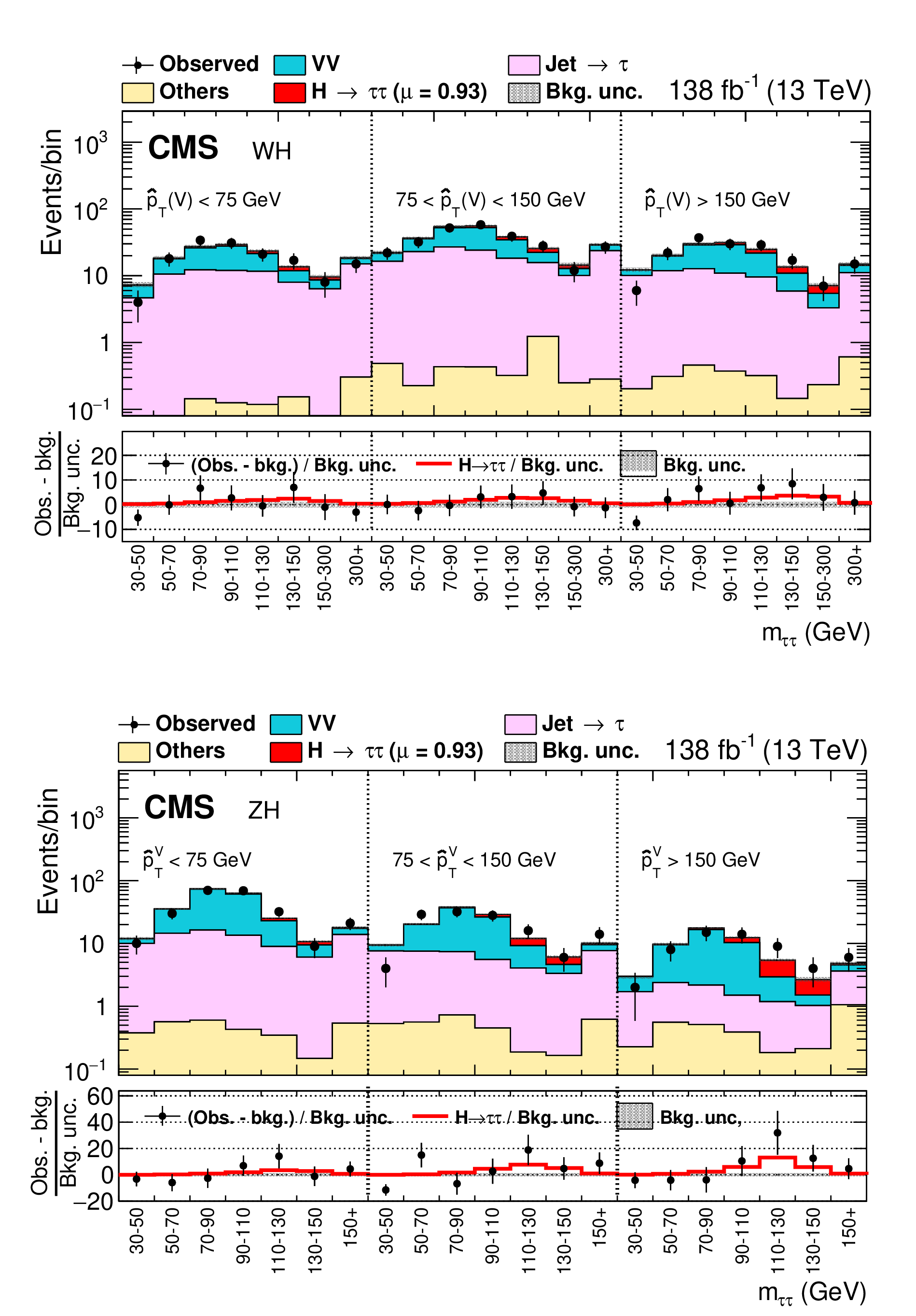
Figure 9:
Observed and predicted distribution of $ m_{ \tau \tau } $ in three bins of $ \hat{p}_{\mathrm{T}}^{ \mathrm{V} } $, combined for all final states and all data-taking years for the (upper) WH and (lower) ZH analyses. |

png pdf |
Figure 9-a:
Observed and predicted distribution of $ m_{ \tau \tau } $ in three bins of $ \hat{p}_{\mathrm{T}}^{ \mathrm{V} } $, combined for all final states and all data-taking years for the WH analysis. |

png pdf |
Figure 9-b:
Observed and predicted distribution of $ m_{ \tau \tau } $ in three bins of $ \hat{p}_{\mathrm{T}}^{ \mathrm{V} } $, combined for all final states and all data-taking years for the ZH analysis. |
png pdf |
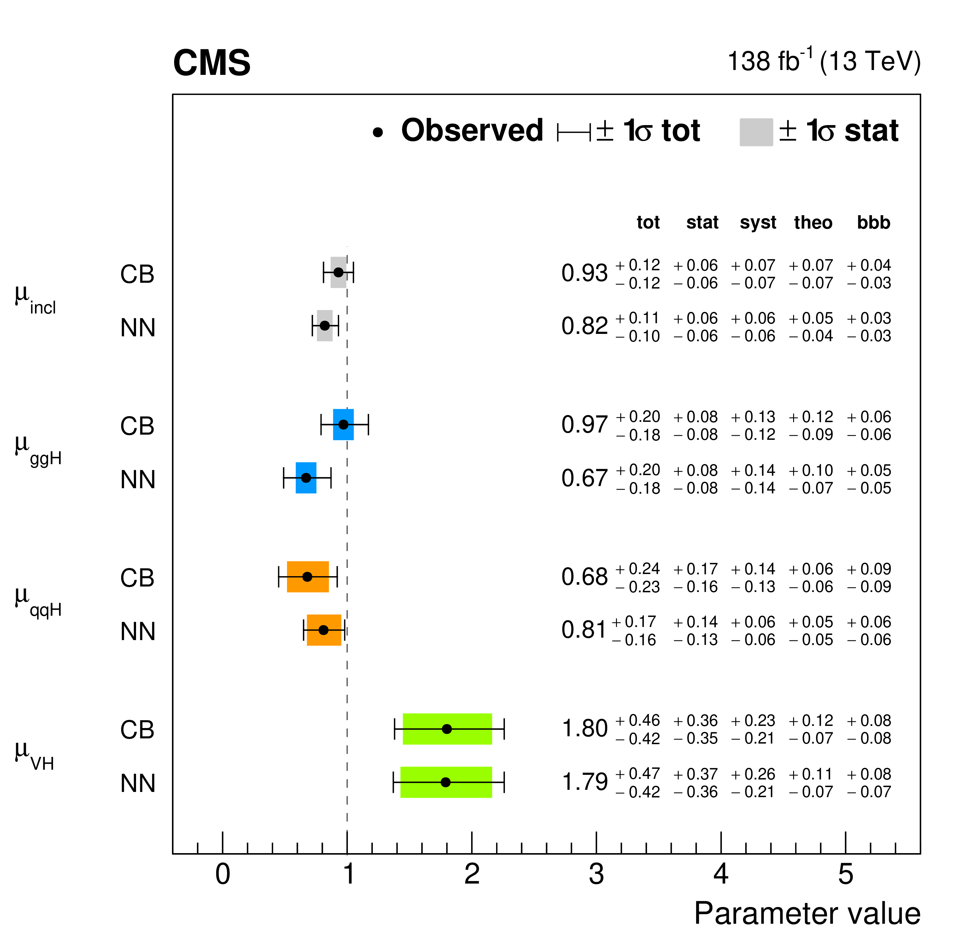
Figure 10:
Measurements of the signal strength parameters for inclusive H production ($ \mu_{\text{incl}} $) and the ggH ($ \mu_{ \mathrm{g} \mathrm{g} \mathrm{H} } $), qqH ($ \mu_{ \mathrm{q} \mathrm{q} \mathrm{H} } $), and VH ($ \mu_{ \mathrm{V} \mathrm{H} } $) STXS stage-0 processes. The combination of the CB- and VH -analyses is labeled by CB. The combination of the NN- and VH -analyses is labeled by NN. Central values maximizing the likelihood and a split of uncertainties as explained in the text are provided with each result. |

png pdf |
Figure 11:
Observed and expected $ m_{ \tau \tau } $ distributions of the analyzed data in all $ \tau \tau $ final states. For the (upper left) CB-, (lower left) WH -, and (lower right) ZH -analyses, $ m_{ \tau \tau } $ from all event categories and data-taking years in a predefined window around the assumed H mass [13] is histogrammed, weighted by the signal (S) over combined background (B) ratio in each event category. For the (upper right) NN-analysis, the events fulfilling $ y_{ \mathrm{g} \mathrm{g} \mathrm{H} } + y_{ \mathrm{q} \mathrm{q} \mathrm{H} } > $ 0.8 are shown without further weight applied. The inclusive contribution of the H signal with $ \mu_{\text{incl}} $ as obtained from the maximum likelihood estimates is also shown, in each subfigure. For the upper right figure $ \mu_{\text{incl}} $ is obtained from the combination of the VH- and the NN-analyses, for the other figures $ \mu_{\text{incl}} $ is obtained from the combination of the VH- and the CB-analyses. |

png pdf |
Figure 11-a:
Observed and expected $ m_{ \tau \tau } $ distributions of the analyzed data in all $ \tau \tau $ final states. For the CB-analysis, $ m_{ \tau \tau } $ from all event categories and data-taking years in a predefined window around the assumed H mass [13] is histogrammed, weighted by the signal (S) over combined background (B) ratio in each event category. The inclusive contribution of the H signal with $ \mu_{\text{incl}} $ as obtained from the maximum likelihood estimates is also shown. $ \mu_{\text{incl}} $ is obtained from the combination of the VH- and the CB-analyses. |

png pdf |
Figure 11-b:
Observed and expected $ m_{ \tau \tau } $ distributions of the analyzed data in all $ \tau \tau $ final states. For the NN-analysis, the events fulfilling $ y_{ \mathrm{g} \mathrm{g} \mathrm{H} } + y_{ \mathrm{q} \mathrm{q} \mathrm{H} } > $ 0.8 are shown without further weight applied. The inclusive contribution of the H signal with $ \mu_{\text{incl}} $ as obtained from the maximum likelihood estimates is also shown. $ \mu_{\text{incl}} $ is obtained from the combination of the VH- and the NN-analyses, |

png pdf |
Figure 11-c:
Observed and expected $ m_{ \tau \tau } $ distributions of the analyzed data in all $ \tau \tau $ final states. For the WH-analysis, $ m_{ \tau \tau } $ from all event categories and data-taking years in a predefined window around the assumed H mass [13] is histogrammed, weighted by the signal (S) over combined background (B) ratio in each event category. The inclusive contribution of the H signal with $ \mu_{\text{incl}} $ as obtained from the maximum likelihood estimates is also shown. $ \mu_{\text{incl}} $ is obtained from the combination of the VH- and the CB-analyses. |

png pdf |
Figure 11-d:
Observed and expected $ m_{ \tau \tau } $ distributions of the analyzed data in all $ \tau \tau $ final states. For ZH-analysis, $ m_{ \tau \tau } $ from all event categories and data-taking years in a predefined window around the assumed H mass [13] is histogrammed, weighted by the signal (S) over combined background (B) ratio in each event category. The inclusive contribution of the H signal with $ \mu_{\text{incl}} $ as obtained from the maximum likelihood estimates is also shown. $ \mu_{\text{incl}} $ is obtained from the combination of the VH- and the CB-analyses. |

png pdf |
Figure 12:
Measurements of the signal strength parameters $\mu_{s}$ in the STXS stage-1.2 bins for the (upper row) ggH, (lower left) qqH, and (lower right) VH processes. The combination of the CB- and VH -analyses is labeled by CB. The combination of the NN- and VH -analyses is labeled by NN. Central values maximizing the likelihood and a split of uncertainties are also provided with each result. |

png pdf |
Figure 12-a:
Measurements of the signal strength parameters $\mu_{s}$ in the STXS stage-1.2 bins for the ggH process. The combination of the CB- and VH -analyses is labeled by CB. The combination of the NN- and VH -analyses is labeled by NN. Central values maximizing the likelihood and a split of uncertainties are also provided with each result. |

png pdf |
Figure 12-b:
Measurements of the signal strength parameters $\mu_{s}$ in the STXS stage-1.2 bins for the ggH process. The combination of the CB- and VH -analyses is labeled by CB. The combination of the NN- and VH -analyses is labeled by NN. Central values maximizing the likelihood and a split of uncertainties are also provided with each result. |

png pdf |
Figure 12-c:
Measurements of the signal strength parameters $\mu_{s}$ in the STXS stage-1.2 bins for the qqH process. The combination of the CB- and VH -analyses is labeled by CB. The combination of the NN- and VH -analyses is labeled by NN. Central values maximizing the likelihood and a split of uncertainties are also provided with each result. |

png pdf |
Figure 12-d:
Measurements of the signal strength parameters $\mu_{s}$ in the STXS stage-1.2 bins for the VH process. The combination of the CB- and VH -analyses is labeled by CB. The combination of the NN- and VH -analyses is labeled by NN. Central values maximizing the likelihood and a split of uncertainties are also provided with each result. |

png pdf |
Figure 13:
Correlation matrices of the POIs of the measured STXS stage-1.2 signal strengths for the combination of the (upper) CB-, resp. (lower) NN-analysis with the VH -analysis. |

png pdf |
Figure 13-a:
Correlation matrices of the POIs of the measured STXS stage-1.2 signal strengths for the combination of the CB-analysis with the VH-analysis. |

png pdf |
Figure 13-b:
Correlation matrices of the POIs of the measured STXS stage-1.2 signal strengths for the combination of the NN-analysis with the VH-analysis. |

png pdf |
Figure 14:
Cross section measurements in the (upper left) stage-0 bins, and in the stage-1.2 bins related to the (lower left) VH, (upper right) qqH, and (lower right) ggH processes. The combination of the CB- and VH -analyses is labeled by CB, the combination of the NN- and VH -analyses is labeled by NN. Central values and combined statistical and systematic uncertainties are given for each measurement. |

png pdf |
Figure 14-a:
Cross section measurements in the (upper) stage-0 bins, and in the stage-1.2 bins related to the (lower) VH, (upper) qqH processes. The combination of the CB- and VH -analyses is labeled by CB, the combination of the NN- and VH -analyses is labeled by NN. Central values and combined statistical and systematic uncertainties are given for each measurement. |

png pdf |
Figure 14-b:
Cross section measurements in the (upper) stage-0 bins, and in the stage-1.2 bins related to the ggH process. The combination of the CB- and VH -analyses is labeled by CB, the combination of the NN- and VH -analyses is labeled by NN. Central values and combined statistical and systematic uncertainties are given for each measurement. |

png pdf |
Figure 15:
Most probable values, 68, and 95% confidence interval contours obtained from a negative log-likelihood scan, for a model treating the H couplings to vector bosons ($ \kappa_{ \mathrm{V} } $) and fermions ($ \kappa_{\mathrm{F}} $) as POIs. The combination of the CB- (NN-) with VH -analyses is shown in light red (dark blue). For the likelihood evaluation all nuisance parameters are profiled in each point in the plane. The $ \mathrm{H} \to \mathrm{W} \mathrm{W} $ decay is treated as signal. |
| Tables | |
png pdf |
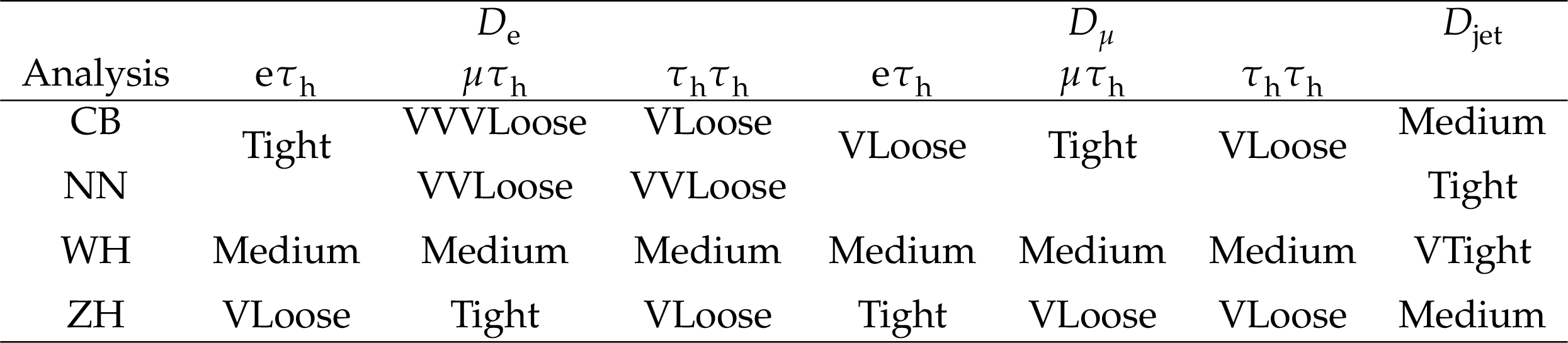
Table 1:
Selected working points for each of the analyses presented in this paper. For each analysis, the working point of $ D_{\text{jet}} $ is the same for all final states. The working points for $ D_{ \mathrm{e} } $ and $ D_{ \mu } $ vary by final state. The labels WH and ZH stand for the individual production modes addressed by the VH -analysis. More details on the efficiency and misidentification rates of the individual working points are given in the text and in Ref. [54]. |

png pdf |
Table 2:
Offline selection requirements applied to the electron, muon, and $ \tau _\mathrm{h} $ candidates used for the selection of the $ \tau $ pair. The expressions first and second lepton refer to the label of the final state in the first column. The $ p_{\mathrm{T}} $ requirements are given in GeV. For the $ \mathrm{e} \mu $ final state two lepton pair trigger paths, with a stronger requirement on the $ p_{\mathrm{T}} $ of electron (muon), are used for the online selection of the event. For the $ \mathrm{e} \tau _\mathrm{h} $ and $ \mu \tau _\mathrm{h} $ final states, the values (in parentheses) correspond to the lepton pair (single lepton) trigger paths that have been used in the online selection. A detailed discussion is given in the text. |
png pdf |
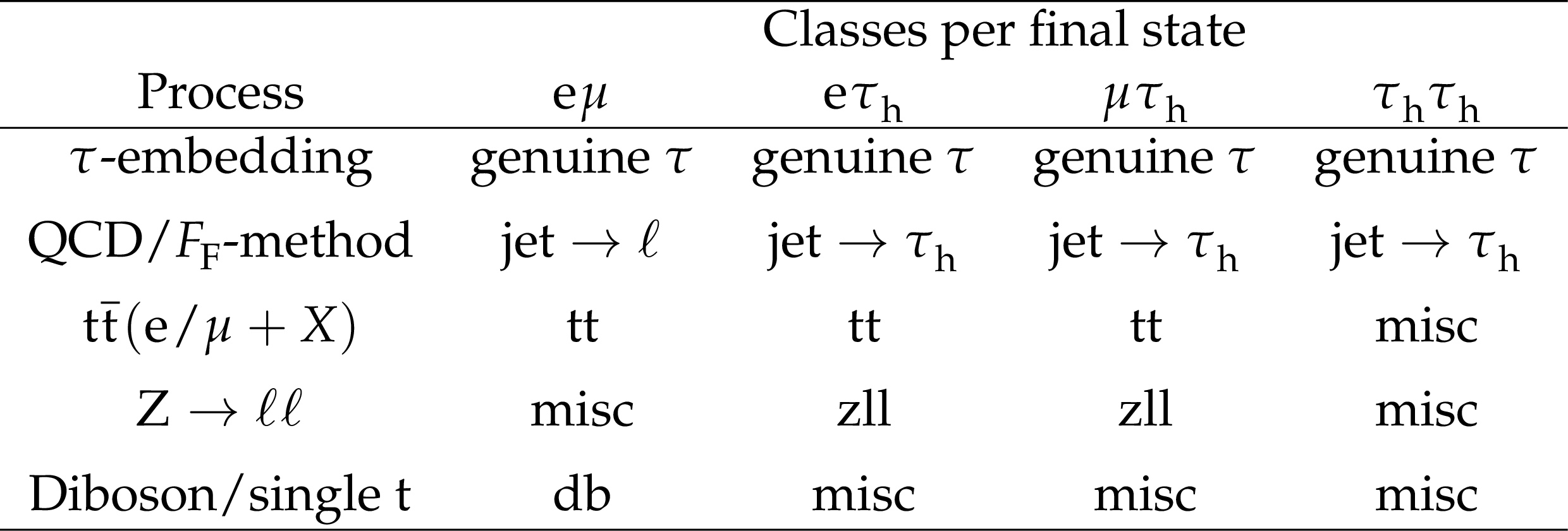
Table 3:
Background processes and event classes for each $ \tau \tau $ final state for the NN-analysis. All event classes enter the NN trainings for the event multiclassification with the same statistical weight (i.e., with uniform prevalence). The label ${ \mathrm{t} \overline{\mathrm{t}} } ( \mathrm{e} / \mu +X)$ refers to the fraction of $\mathrm{t \bar{t}}$ production that is not covered by any of the estimation methods from data, as listed in the first two rows. The classes tt, misc, zll, and db are defined in the introduction of Section 7. |

png pdf |
Table 4:
Event categories of the CB-analysis. The STXS stage-0 and -1.2 measurements are extracted by performing a maximum likelihood fit of 1D and 2D distributions in these categories using the observables listed in the last column. |

png pdf |
Table 5:
Selection requirements for $ \mathrm{e} $, $ \mu $ and $ \tau _\mathrm{h} $ candidates used in the WH analysis. The three $ p_{\mathrm{T}} $ thresholds specified for the $ \mathrm{e} $ in the $ \mathrm{e} \tau _\mathrm{h} \tau _\mathrm{h} $ final state refer to the years 2016, 2017, and 2018, respectively. The column labeled $ I_{\text{rel}}^{ \mathrm{e} ( \mu )} $ refers to the lepton isolation variable, defined in Eq. (1). |

png pdf |
Table 6:
Selection requirements for $ \mathrm{e} $ and $ \mu $ candidates that are associated with the $ \mathrm{Z} \to \ell \ell $ decay in the ZH analysis. The three $ p_{\mathrm{T}} $ thresholds and the three $\eta$ restrictions specified for the triggering leptons refer to the years 2016, 2017, and 2018, respectively. The column labeled $ I_{\text{rel}}^{ \mathrm{e} ( \mu )} $ refers to the lepton isolation variable, defined in Eq. (1). |

png pdf |
Table 7:
Selection requirements for $ \mathrm{e} $, $ \mu $, and $ \tau _\mathrm{h} $ candidates associated with the $ \tau \tau $ decay in the ZH analysis. First and second lepton refers to the label of the final state in the first column. The column labeled $ I_{\text{rel}}^{ \mathrm{e} ( \mu )} $ refers to the lepton isolation variable, defined in Eq. (1). |

png pdf |
Table 8:
Summary of the most important systematic uncertainties discussed in the text. The columns indicate the source of uncertainty, the process class that it applies to, the variation, and how it is correlated. A checkmark is given also for partial correlations. More details are given in the text. |

png pdf |
Table 9:
Tabulated values of the STXS stage-0 and -1.2 signal strengths for the combination of the (CB) CB-, resp. (NN) NN-analysis with the VH -analysis. The upper four lines refer to the inclusive and STXS stage-0 measurements. The values in braces correspond to the expected 68% confidence intervals for an assumed SM signal. The products of cross sections and branching fraction to $ \tau $ leptons as expected from the SM with the uncertainties as discussed in Section 4 are also given. |
| Summary |
| Measurements of Higgs boson production, where the Higgs boson decays into a pair of $ \tau $ leptons, have been presented. The analyzed data are selected from proton-proton collisions at a center-of-mass energy of 13 TeV collected by the CMS experiment at the LHC from 2016--2018, corresponding to an integrated luminosity of 138 fb$^{-1}$. Results are presented in the form of signal strengths relative to the standard model predictions and products of cross sections and branching fraction to $ \tau $ leptons, in up to 16 different kinematic regions, following the simplified template cross section scheme of the LHC Higgs Working Group. For the simultaneous measurements of a neural network based analysis and an analysis targeting vector boson associated Higgs boson production signal strengths are found to be 0.82 $ \pm $ 0.11 for inclusive Higgs boson production, 0.67 $ \pm $ 0.19 (0.81 $ \pm $ 0.17) for the production mainly via gluon fusion (vector boson fusion), and 1.79 $ \pm $ 0.45 for vector boson associated Higgs boson production. The latter result significantly improves an earlier measurement performed by the CMS Collaboration on a smaller data set. |
| Additional Figures | |

png pdf |
Additional Figure 1:
Observed and expected distributions of the NN output function $ y_{l} $ in the signal class of the ggH STXS stage-1.2 bin with $ \text{0 jet},\, p_{\mathrm{T}} ^{ \mathrm{H} } [0, 10] $ GeV in the $ \mu \tau _\mathrm{h} $ final state. The signal contributions for (red) the corresponding STXS bin, and for the remaining inclusive (blue) ggH and (orange) qqH processes, excluding the STXS bin in consideration are also shown as unstacked open histograms. All distributions are shown after the fit of the model, used for the extraction of the STXS stage-1.2 signals, to the data from all final states and data-taking years. Signal contributions in particular have been scaled according to the obtained fit results. |

png pdf |
Additional Figure 2:
Observed and expected distributions of the NN output function $ y_{l} $ in the signal class of the ggH STXS stage-1.2 bin with $ \text{0 jet},\, p_{\mathrm{T}} ^{ \mathrm{H} } [10, 200] $ GeV for all data-taking years, in the $ \mu \tau _\mathrm{h} $ final state. The signal contributions for (red) the corresponding STXS bin, and for the remaining inclusive (blue) ggH and (orange) qqH processes, excluding the STXS bin in consideration are also shown as unstacked open histograms. All distributions are shown after the fit of the model, used for the extraction of the STXS stage-1.2 signals, to the data from all final states and data-taking years. Signal contributions in particular have been scaled according to the obtained fit results. |

png pdf |
Additional Figure 3:
Observed and expected distributions of the NN output function $ y_{l} $ in the signal class of the ggH STXS stage-1.2 bin with $ \geq\text{2 jet},\, m_{\mathrm{jj}} \geq$ 350 GeV, $ p_{\mathrm{T}} ^{ \mathrm{H} } [0, 200] $ GeV in the $ \mu \tau _\mathrm{h} $ final state. The signal contributions for (red) the corresponding STXS bin, and for the remaining inclusive (blue) ggH and (orange) qqH processes, excluding the STXS bin in consideration are also shown as unstacked open histograms. All distributions are shown after the fit of the model, used for the extraction of the STXS stage-1.2 signals, to the data from all final states and data-taking years. Signal contributions in particular have been scaled according to the obtained fit results. |

png pdf |
Additional Figure 4:
Observed and expected distributions of the NN output function $ y_{l} $ in the signal class of the qqH STXS stage-1.2 bin with $ \geq\text{2 jet},\, m_{\mathrm{jj}} \geq$ 700 GeV, $ p_{\mathrm{T}} ^{ \mathrm{H} } [0, 200] $ GeV in the $ \mu \tau _\mathrm{h} $ final state. The signal contributions for (red) the corresponding STXS bin, and for the remaining inclusive (blue) ggH and (orange) qqH processes, excluding the STXS bin in consideration are also shown as unstacked open histograms. All distributions are shown after the fit of the model, used for the extraction of the STXS stage-1.2 signals, to the data from all final states and data-taking years. Signal contributions in particular have been scaled according to the obtained fit results. |

png pdf |
Additional Figure 5:
Observed and expected distributions of the NN output function $ y_{l} $ in the signal class of the ggH STXS stage-1.2 bin with $ \text{0 jet},\, p_{\mathrm{T}} ^{ \mathrm{H} } [0, 10] $ GeV in the $ \tau _\mathrm{h} \tau _\mathrm{h} $ final state. The signal contributions for (red) the corresponding STXS bin, and for the remaining inclusive (blue) ggH and (orange) qqH processes, excluding the STXS bin in consideration are also shown as unstacked open histograms. All distributions are shown after the fit of the model, used for the extraction of the STXS stage-1.2 signals, to the data from all final states and data-taking years. Signal contributions in particular have been scaled according to the obtained fit results. |

png pdf |
Additional Figure 6:
Observed and expected distributions of the NN output function $ y_{l} $ in the signal class of the ggH STXS stage-1.2 bin with $ \text{0 jet},\, p_{\mathrm{T}} ^{ \mathrm{H} } [10, 200] $ GeV in the $ \tau _\mathrm{h} \tau _\mathrm{h} $ final state. The signal contributions for (red) the corresponding STXS bin, and for the remaining inclusive (blue) ggH and (orange) qqH processes, excluding the STXS bin in consideration are also shown as unstacked open histograms. All distributions are shown after the fit of the model, used for the extraction of the STXS stage-1.2 signals, to the data from all final states and data-taking years. Signal contributions in particular have been scaled according to the obtained fit results. |
png pdf |
Additional Figure 7:
Observed and expected distributions of the NN output function $ y_{l} $ in the signal class of the ggH STXS stage-1.2 bin with $ \text{1 jet},\, p_{\mathrm{T}} ^{ \mathrm{H} } [0, 60] $ GeV in the $ \tau _\mathrm{h} \tau _\mathrm{h} $ final state. The signal contributions for (red) the corresponding STXS bin, and for the remaining inclusive (blue) ggH and (orange) qqH processes, excluding the STXS bin in consideration are also shown as unstacked open histograms. All distributions are shown after the fit of the model, used for the extraction of the STXS stage-1.2 signals, to the data from all final states and data-taking years. Signal contributions in particular have been scaled according to the obtained fit results. |
png pdf |
Additional Figure 8:
Observed and expected distributions of the NN output function $ y_{l} $ in the signal class of the ggH STXS stage-1.2 bin with $ \text{1 jet},\, p_{\mathrm{T}} ^{ \mathrm{H} } [60, 120] $ GeV in the $ \tau _\mathrm{h} \tau _\mathrm{h} $ final state. The signal contributions for (red) the corresponding STXS bin, and for the remaining inclusive (blue) ggH and (orange) qqH processes, excluding the STXS bin in consideration are also shown as unstacked open histograms. All distributions are shown after the fit of the model, used for the extraction of the STXS stage-1.2 signals, to the data from all final states and data-taking years. Signal contributions in particular have been scaled according to the obtained fit results. |

png pdf |
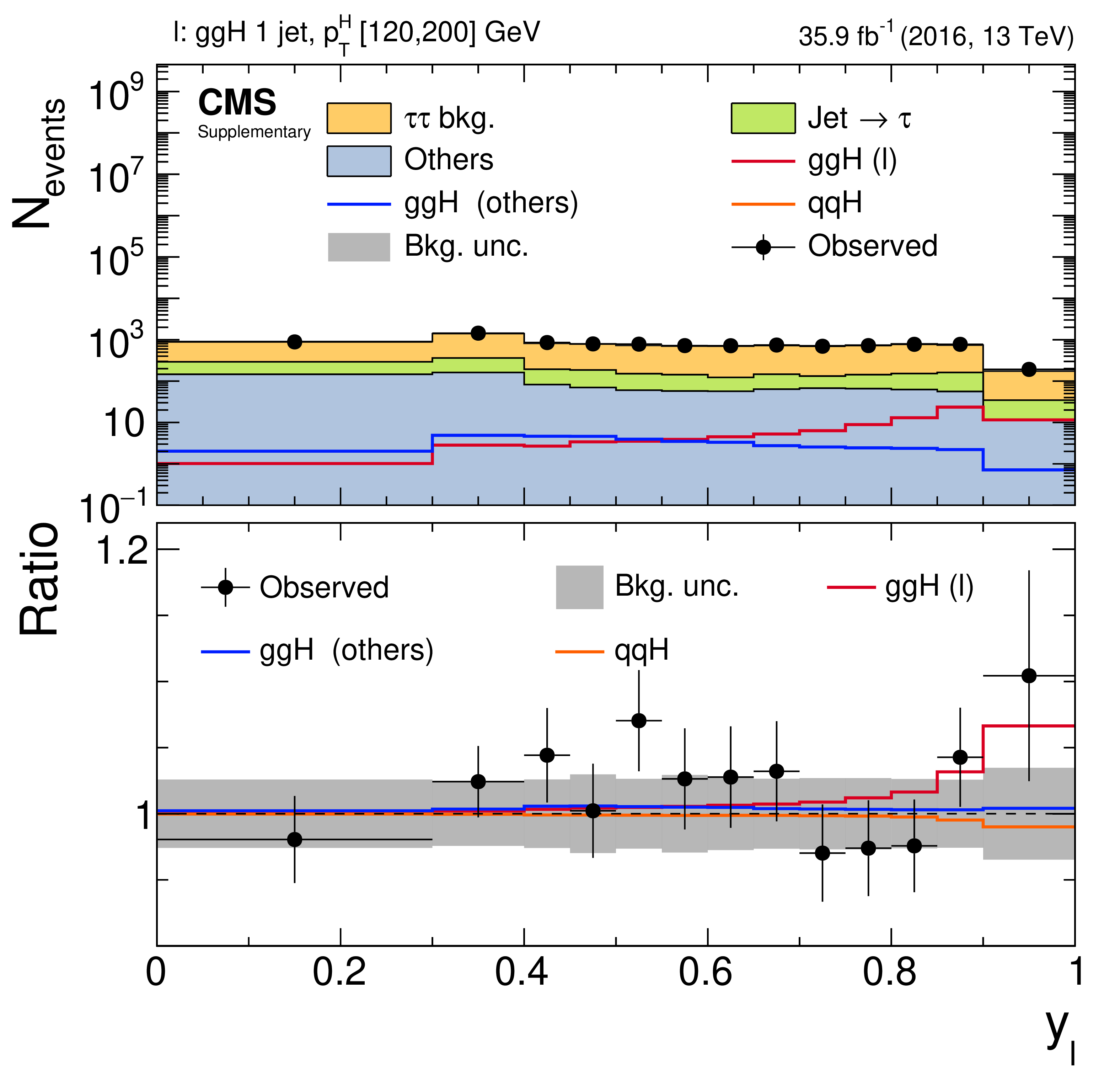
Additional Figure 9:
Observed and expected distributions of the NN output function $ y_{l} $ in the signal class of the ggH STXS stage-1.2 bin with $ \text{1 jet},\, p_{\mathrm{T}} ^{ \mathrm{H} } [120, 200] $ GeV in the $ \tau _\mathrm{h} \tau _\mathrm{h} $ final state. The signal contributions for (red) the corresponding STXS bin, and for the remaining inclusive (blue) ggH and (orange) qqH processes, excluding the STXS bin in consideration are also shown as unstacked open histograms. All distributions are shown after the fit of the model, used for the extraction of the STXS stage-1.2 signals, to the data from all final states and data-taking years. Signal contributions in particular have been scaled according to the obtained fit results. |

png pdf |
Additional Figure 10:
Observed and expected distributions of the NN output function $ y_{l} $ in the signal class of the ggH STXS stage-1.2 bin with $ \geq\text{2 jet},\, m_{\mathrm{jj}} \geq$ 350 GeV, $ p_{\mathrm{T}} ^{ \mathrm{H} } [0, 200] $ GeV in the $ \tau _\mathrm{h} \tau _\mathrm{h} $ final state. The signal contributions for (red) the corresponding STXS bin, and for the remaining inclusive (blue) ggH and (orange) qqH processes, excluding the STXS bin in consideration are also shown as unstacked open histograms. All distributions are shown after the fit of the model, used for the extraction of the STXS stage-1.2 signals, to the data from all final states and data-taking years. Signal contributions in particular have been scaled according to the obtained fit results. |

png pdf |
Additional Figure 11:
Observed and expected distributions of the NN output function $ y_{l} $ in the signal class of the qqH STXS stage-1.2 bin with $ \geq\text{2 jet},\, m_{\mathrm{jj}} [350, 700] $ GeV, $ p_{\mathrm{T}} ^{ \mathrm{H} } [0, 200] $ GeV in the $ \tau _\mathrm{h} \tau _\mathrm{h} $ final state. The signal contributions for (red) the corresponding STXS bin, and for the remaining inclusive (blue) ggH and (orange) qqH processes, excluding the STXS bin in consideration are also shown as unstacked open histograms. All distributions are shown after the fit of the model, used for the extraction of the STXS stage-1.2 signals, to the data from all final states and data-taking years. Signal contributions in particular have been scaled according to the obtained fit results. |

png pdf |
Additional Figure 12:
Observed and expected distributions of the NN output function $ y_{l} $ in the signal class of the qqH STXS stage-1.2 bin with $ \geq\text{2 jet},\, m_{\mathrm{jj}} \geq$ 700 GeV, $ p_{\mathrm{T}} ^{ \mathrm{H} } [0, 200] $ GeV in the $ \tau _\mathrm{h} \tau _\mathrm{h} $ final state. The signal contributions for (red) the corresponding STXS bin, and for the remaining inclusive (blue) ggH and (orange) qqH processes, excluding the STXS bin in consideration are also shown as unstacked open histograms. All distributions are shown after the fit of the model, used for the extraction of the STXS stage-1.2 signals, to the data from all final states and data-taking years. Signal contributions in particular have been scaled according to the obtained fit results. |

png pdf |
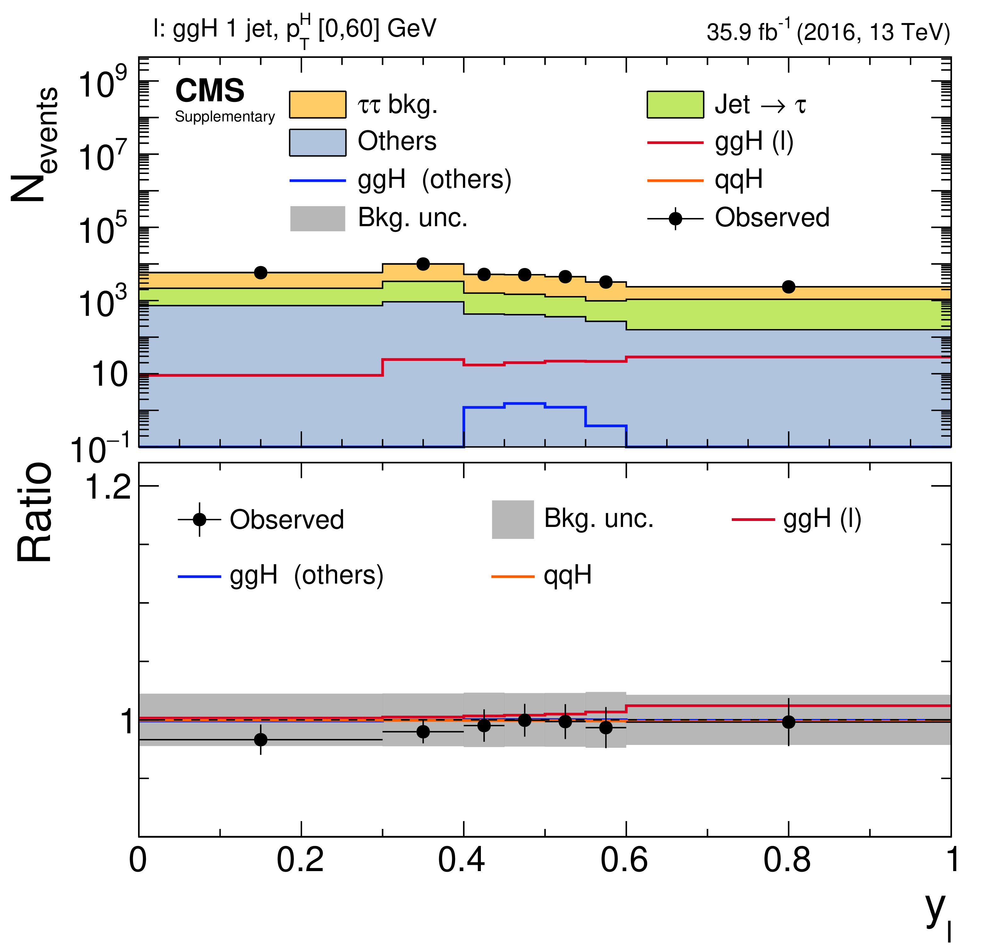
Additional Figure 13:
Observed and expected distributions of the NN output function $ y_{l} $ in the signal class of the ggH STXS stage-1.2 bin with $ \text{0 jet},\, p_{\mathrm{T}} ^{ \mathrm{H} } [0, 10] $ GeV for all final states and the data taken in 2016. The signal contributions for (red) the corresponding STXS bin, and for the remaining inclusive (blue) ggH and (orange) qqH processes, excluding the STXS bin in consideration are also shown as unstacked open histograms. All distributions are shown after the fit of the model, used for the extraction of the STXS stage-1.2 signals, to the data from all final states and data-taking years. Signal contributions in particular have been scaled according to the obtained fit results. |

png pdf |
Additional Figure 14:
Observed and expected distributions of the NN output function $ y_{l} $ in the signal class of the ggH STXS stage-1.2 bin with $ \text{0 jet},\, p_{\mathrm{T}} ^{ \mathrm{H} } [10, 200] $ GeV for all final states and the data taken in 2016. The signal contributions for (red) the corresponding STXS bin, and for the remaining inclusive (blue) ggH and (orange) qqH processes, excluding the STXS bin in consideration are also shown as unstacked open histograms. All distributions are shown after the fit of the model, used for the extraction of the STXS stage-1.2 signals, to the data from all final states and data-taking years. Signal contributions in particular have been scaled according to the obtained fit results. |
png pdf |
Additional Figure 15:
Observed and expected distributions of the NN output function $ y_{l} $ in the signal class of the ggH STXS stage-1.2 bin with $ \text{1 jet},\, p_{\mathrm{T}} ^{ \mathrm{H} } [0, 60] $ GeV for all final states and the data taken in 2016. The signal contributions for (red) the corresponding STXS bin, and for the remaining inclusive (blue) ggH and (orange) qqH processes, excluding the STXS bin in consideration are also shown as unstacked open histograms. All distributions are shown after the fit of the model, used for the extraction of the STXS stage-1.2 signals, to the data from all final states and data-taking years. Signal contributions in particular have been scaled according to the obtained fit results. |

png pdf |
Additional Figure 16:
Observed and expected distributions of the NN output function $ y_{l} $ in the signal class of the ggH STXS stage-1.2 bin with $ \text{1 jet},\, p_{\mathrm{T}} ^{ \mathrm{H} } [60, 120] $ GeV for all final states and the data taken in 2016. The signal contributions for (red) the corresponding STXS bin, and for the remaining inclusive (blue) ggH and (orange) qqH processes, excluding the STXS bin in consideration are also shown as unstacked open histograms. All distributions are shown after the fit of the model, used for the extraction of the STXS stage-1.2 signals, to the data from all final states and data-taking years. Signal contributions in particular have been scaled according to the obtained fit results. |
png pdf |
Additional Figure 17:
Observed and expected distributions of the NN output function $ y_{l} $ in the signal class of the ggH STXS stage-1.2 bin with $ \text{1 jet},\, p_{\mathrm{T}} ^{ \mathrm{H} } [120, 200] $ GeV for all final states and the data taken in 2016. The signal contributions for (red) the corresponding STXS bin, and for the remaining inclusive (blue) ggH and (orange) qqH processes, excluding the STXS bin in consideration are also shown as unstacked open histograms. All distributions are shown after the fit of the model, used for the extraction of the STXS stage-1.2 signals, to the data from all final states and data-taking years. Signal contributions in particular have been scaled according to the obtained fit results. |

png pdf |
Additional Figure 18:
Observed and expected distributions of the NN output function $ y_{l} $ in the signal class of the ggH STXS stage-1.2 bin with $ \geq\text{2 jet},\, m_{\mathrm{jj}} \geq$ 350 GeV, $ p_{\mathrm{T}} ^{ \mathrm{H} } [0, 200] $ GeV for all final states and the data taken in 2016. The signal contributions for (red) the corresponding STXS bin, and for the remaining inclusive (blue) ggH and (orange) qqH processes, excluding the STXS bin in consideration are also shown as unstacked open histograms. All distributions are shown after the fit of the model, used for the extraction of the STXS stage-1.2 signals, to the data from all final states and data-taking years. Signal contributions in particular have been scaled according to the obtained fit results. |

png pdf |
Additional Figure 19:
Observed and expected distributions of the NN output function $ y_{l} $ in the signal class of the qqH STXS stage-1.2 bin with $ \geq\text{2 jet},\, m_{\mathrm{jj}} [350, 700] $ GeV, $ p_{\mathrm{T}} ^{ \mathrm{H} } [0, 200] $ GeV for all final states and the data taken in 2016. The signal contributions for (red) the corresponding STXS bin, and for the remaining inclusive (blue) ggH and (orange) qqH processes, excluding the STXS bin in consideration are also shown as unstacked open histograms. All distributions are shown after the fit of the model, used for the extraction of the STXS stage-1.2 signals, to the data from all final states and data-taking years. Signal contributions in particular have been scaled according to the obtained fit results. |

png pdf |
Additional Figure 20:
Observed and expected distributions of the NN output function $ y_{l} $ in the signal class of the qqH STXS stage-1.2 bin with $ \geq\text{2 jet},\, m_{\mathrm{jj}} \geq$ 700 GeV, $ p_{\mathrm{T}} ^{ \mathrm{H} } [0, 200] $ GeV for all final states and the data taken in 2016. The signal contributions for (red) the corresponding STXS bin, and for the remaining inclusive (blue) ggH and (orange) qqH processes, excluding the STXS bin in consideration are also shown as unstacked open histograms. All distributions are shown after the fit of the model, used for the extraction of the STXS stage-1.2 signals, to the data from all final states and data-taking years. Signal contributions in particular have been scaled according to the obtained fit results. |
png pdf |
Additional Figure 21:
Observed and expected distributions of the NN output function $ y_{l} $ in the signal class of the ggH STXS stage-1.2 bin with $ \text{0 jet},\, p_{\mathrm{T}} ^{ \mathrm{H} } [0, 10] $ GeV for all final states and the data taken in 2017. The signal contributions for (red) the corresponding STXS bin, and for the remaining inclusive (blue) ggH and (orange) qqH processes, excluding the STXS bin in consideration are also shown as unstacked open histograms. All distributions are shown after the fit of the model, used for the extraction of the STXS stage-1.2 signals, to the data from all final states and data-taking years. Signal contributions in particular have been scaled according to the obtained fit results. |

png pdf |
Additional Figure 22:
Observed and expected distributions of the NN output function $ y_{l} $ in the signal class of the ggH STXS stage-1.2 bin with $ \text{0 jet},\, p_{\mathrm{T}} ^{ \mathrm{H} } [10, 200] $ GeV for all final states and the data taken in 2017. The signal contributions for (red) the corresponding STXS bin, and for the remaining inclusive (blue) ggH and (orange) qqH processes, excluding the STXS bin in consideration are also shown as unstacked open histograms. All distributions are shown after the fit of the model, used for the extraction of the STXS stage-1.2 signals, to the data from all final states and data-taking years. Signal contributions in particular have been scaled according to the obtained fit results. |

png pdf |
Additional Figure 23:
Observed and expected distributions of the NN output function $ y_{l} $ in the signal class of the ggH STXS stage-1.2 bin with $ \text{1 jet},\, p_{\mathrm{T}} ^{ \mathrm{H} } [0, 60] $ GeV for all final states and the data taken in 2017. The signal contributions for (red) the corresponding STXS bin, and for the remaining inclusive (blue) ggH and (orange) qqH processes, excluding the STXS bin in consideration are also shown as unstacked open histograms. All distributions are shown after the fit of the model, used for the extraction of the STXS stage-1.2 signals, to the data from all final states and data-taking years. Signal contributions in particular have been scaled according to the obtained fit results. |

png pdf |
Additional Figure 24:
Observed and expected distributions of the NN output function $ y_{l} $ in the signal class of the ggH STXS stage-1.2 bin with $ \text{1 jet},\, p_{\mathrm{T}} ^{ \mathrm{H} } [60, 120] $ GeV for all final states and the data taken in 2017. The signal contributions for (red) the corresponding STXS bin, and for the remaining inclusive (blue) ggH and (orange) qqH processes, excluding the STXS bin in consideration are also shown as unstacked open histograms. All distributions are shown after the fit of the model, used for the extraction of the STXS stage-1.2 signals, to the data from all final states and data-taking years. Signal contributions in particular have been scaled according to the obtained fit results. |

png pdf |
Additional Figure 25:
Observed and expected distributions of the NN output function $ y_{l} $ in the signal class of the ggH STXS stage-1.2 bin with $ \text{1 jet},\, p_{\mathrm{T}} ^{ \mathrm{H} } [120, 200] $ GeV for all final states and the data taken in 2017. The signal contributions for (red) the corresponding STXS bin, and for the remaining inclusive (blue) ggH and (orange) qqH processes, excluding the STXS bin in consideration are also shown as unstacked open histograms. All distributions are shown after the fit of the model, used for the extraction of the STXS stage-1.2 signals, to the data from all final states and data-taking years. Signal contributions in particular have been scaled according to the obtained fit results. |

png pdf |
Additional Figure 26:
Observed and expected distributions of the NN output function $ y_{l} $ in the signal class of the ggH STXS stage-1.2 bin with $ \geq\text{2 jet},\, m_{\mathrm{jj}} \geq$ 350 GeV, $ p_{\mathrm{T}} ^{ \mathrm{H} } [0, 200] $ GeV for all final states and the data taken in 2017. The signal contributions for (red) the corresponding STXS bin, and for the remaining inclusive (blue) ggH and (orange) qqH processes, excluding the STXS bin in consideration are also shown as unstacked open histograms. All distributions are shown after the fit of the model, used for the extraction of the STXS stage-1.2 signals, to the data from all final states and data-taking years. Signal contributions in particular have been scaled according to the obtained fit results. |

png pdf |
Additional Figure 27:
Observed and expected distributions of the NN output function $ y_{l} $ in the signal class of the qqH STXS stage-1.2 bin with $ \geq\text{2 jet},\, m_{\mathrm{jj}} [350, 700] $ GeV, $ p_{\mathrm{T}} ^{ \mathrm{H} } [0, 200] $ GeV for all final states and the data taken in 2017. The signal contributions for (red) the corresponding STXS bin, and for the remaining inclusive (blue) ggH and (orange) qqH processes, excluding the STXS bin in consideration are also shown as unstacked open histograms. All distributions are shown after the fit of the model, used for the extraction of the STXS stage-1.2 signals, to the data from all final states and data-taking years. Signal contributions in particular have been scaled according to the obtained fit results. |
png pdf |
Additional Figure 28:
Observed and expected distributions of the NN output function $ y_{l} $ in the signal class of the qqH STXS stage-1.2 bin with $ \geq\text{2 jet},\, m_{\mathrm{jj}} \geq$ 700 GeV, $ p_{\mathrm{T}} ^{ \mathrm{H} } [0, 200] $ GeV for all final states and the data taken in 2017. The signal contributions for (red) the corresponding STXS bin, and for the remaining inclusive (blue) ggH and (orange) qqH processes, excluding the STXS bin in consideration are also shown as unstacked open histograms. All distributions are shown after the fit of the model, used for the extraction of the STXS stage-1.2 signals, to the data from all final states and data-taking years. Signal contributions in particular have been scaled according to the obtained fit results. |
png pdf |
Additional Figure 29:
Observed and expected distributions of the NN output function $ y_{l} $ in the signal class of the ggH STXS stage-1.2 bin with $ \text{0 jet},\, p_{\mathrm{T}} ^{ \mathrm{H} } [0, 10] $ GeV for all final states and the data taken in 2018. The signal contributions for (red) the corresponding STXS bin, and for the remaining inclusive (blue) ggH and (orange) qqH processes, excluding the STXS bin in consideration are also shown as unstacked open histograms. All distributions are shown after the fit of the model, used for the extraction of the STXS stage-1.2 signals, to the data from all final states and data-taking years. Signal contributions in particular have been scaled according to the obtained fit results. |

png pdf |
Additional Figure 30:
Observed and expected distributions of the NN output function $ y_{l} $ in the signal class of the ggH STXS stage-1.2 bin with $ \text{0 jet},\, p_{\mathrm{T}} ^{ \mathrm{H} } [10, 200] $ GeV for all final states and the data taken in 2018. The signal contributions for (red) the corresponding STXS bin, and for the remaining inclusive (blue) ggH and (orange) qqH processes, excluding the STXS bin in consideration are also shown as unstacked open histograms. All distributions are shown after the fit of the model, used for the extraction of the STXS stage-1.2 signals, to the data from all final states and data-taking years. Signal contributions in particular have been scaled according to the obtained fit results. |

png pdf |
Additional Figure 31:
Observed and expected distributions of the NN output function $ y_{l} $ in the signal class of the ggH STXS stage-1.2 bin with $ \text{1 jet},\, p_{\mathrm{T}} ^{ \mathrm{H} } [0, 60] $ GeV for all final states and the data taken in 2018. The signal contributions for (red) the corresponding STXS bin, and for the remaining inclusive (blue) ggH and (orange) qqH processes, excluding the STXS bin in consideration are also shown as unstacked open histograms. All distributions are shown after the fit of the model, used for the extraction of the STXS stage-1.2 signals, to the data from all final states and data-taking years. Signal contributions in particular have been scaled according to the obtained fit results. |

png pdf |
Additional Figure 32:
Observed and expected distributions of the NN output function $ y_{l} $ in the signal class of the ggH STXS stage-1.2 bin with $ \text{1 jet},\, p_{\mathrm{T}} ^{ \mathrm{H} } [60, 120] $ GeV for all final states and the data taken in 2018. The signal contributions for (red) the corresponding STXS bin, and for the remaining inclusive (blue) ggH and (orange) qqH processes, excluding the STXS bin in consideration are also shown as unstacked open histograms. All distributions are shown after the fit of the model, used for the extraction of the STXS stage-1.2 signals, to the data from all final states and data-taking years. Signal contributions in particular have been scaled according to the obtained fit results. |

png pdf |
Additional Figure 33:
Observed and expected distributions of the NN output function $ y_{l} $ in the signal class of the ggH STXS stage-1.2 bin with $ \text{1 jet},\, p_{\mathrm{T}} ^{ \mathrm{H} } [120, 200] $ GeV for all final states and the data taken in 2018. The signal contributions for (red) the corresponding STXS bin, and for the remaining inclusive (blue) ggH and (orange) qqH processes, excluding the STXS bin in consideration are also shown as unstacked open histograms. All distributions are shown after the fit of the model, used for the extraction of the STXS stage-1.2 signals, to the data from all final states and data-taking years. Signal contributions in particular have been scaled according to the obtained fit results. |

png pdf |
Additional Figure 34:
Observed and expected distributions of the NN output function $ y_{l} $ in the signal class of the ggH STXS stage-1.2 bin with $ \geq\text{2 jet},\, m_{\mathrm{jj}} \geq$ 350 GeV, $ p_{\mathrm{T}} ^{ \mathrm{H} } [0, 200] $ GeV for all final states and the data taken in 2018. The signal contributions for (red) the corresponding STXS bin, and for the remaining inclusive (blue) ggH and (orange) qqH processes, excluding the STXS bin in consideration are also shown as unstacked open histograms. All distributions are shown after the fit of the model, used for the extraction of the STXS stage-1.2 signals, to the data from all final states and data-taking years. Signal contributions in particular have been scaled according to the obtained fit results. |

png pdf |
Additional Figure 35:
Observed and expected distributions of the NN output function $ y_{l} $ in the signal class of the qqH STXS stage-1.2 bin with $ \geq\text{2 jet},\, m_{\mathrm{jj}} [350, 700] $ GeV, $ p_{\mathrm{T}} ^{ \mathrm{H} } [0, 200] $ GeV for all final states and the data taken in 2018. The signal contributions for (red) the corresponding STXS bin, and for the remaining inclusive (blue) ggH and (orange) qqH processes, excluding the STXS bin in consideration are also shown as unstacked open histograms. All distributions are shown after the fit of the model, used for the extraction of the STXS stage-1.2 signals, to the data from all final states and data-taking years. Signal contributions in particular have been scaled according to the obtained fit results. |

png pdf |
Additional Figure 36:
Observed and expected distributions of the NN output function $ y_{l} $ in the signal class of the qqH STXS stage-1.2 bin with $ \geq\text{2 jet},\, m_{\mathrm{jj}} \geq$ 700 GeV, $ p_{\mathrm{T}} ^{ \mathrm{H} } [0, 200] $ GeV for all final states and the data taken in 2018. The signal contributions for (red) the corresponding STXS bin, and for the remaining inclusive (blue) ggH and (orange) qqH processes, excluding the STXS bin in consideration are also shown as unstacked open histograms. All distributions are shown after the fit of the model, used for the extraction of the STXS stage-1.2 signals, to the data from all final states and data-taking years. Signal contributions in particular have been scaled according to the obtained fit results. |
png pdf |
Additional Figure 37:
Observed and expected distributions of the NN output function $ y_{l} $ in the genuine $ \tau $ class for all data-taking years, in the $ \mu \tau _\mathrm{h} $ final state. All distributions are shown after the fit of the model, used for the extraction of the inclusive signal, to the data from all final states and data-taking years. |

png pdf |
Additional Figure 38:
Observed and expected distributions of the NN output function $ y_{l} $ in the tt class for all data-taking years, in the $ \mu \tau _\mathrm{h} $ final state. All distributions are shown after the fit of the model, used for the extraction of the inclusive signal, to the data from all final states and data-taking years. |

png pdf |
Additional Figure 39:
Observed and expected distributions of the NN output function $ y_{l} $ in the zll class for all data-taking years, in the $ \mu \tau _\mathrm{h} $ final state. All distributions are shown after the fit of the model, used for the extraction of the inclusive signal, to the data from all final states and data-taking years. |

png pdf |
Additional Figure 40:
Observed and expected distributions of the NN output function $ y_{l} $ in the misc class for all data-taking years, in the $ \mu \tau _\mathrm{h} $ final state. All distributions are shown after the fit of the model, used for the extraction of the inclusive signal, to the data from all final states and data-taking years. |

png pdf |
Additional Figure 41:
Observed and expected distributions of the NN output function $ y_{l} $ in the $ \text{jet}\to \tau _\mathrm{h} $ class for all data-taking years, in the $ \mu \tau _\mathrm{h} $ final state. All distributions are shown after the fit of the model, used for the extraction of the inclusive signal, to the data from all final states and data-taking years. |
png pdf |
Additional Figure 42:
Observed and expected distributions of the 2D discriminant as used for the extraction of the STXS stage-0 and inclusive signals, for all data-taking years in the $ \tau _\mathrm{h} \tau _\mathrm{h} $ final state. The background distributions are shown after the fit of the model, used for the extraction of the inclusive signal, to the data from all final states and data-taking years. The signal contributions for the (red) inclusive, (blue) ggH, and (orange) qqH signals are also shown as unstacked open histograms, scaled according to the correspondingly obtained fit results. The vertical gray dashed lines indicate six primary bins in $ y_\text{qqH} $, the last four of which to the right have been enhanced by factors 5 --25 for improved visibility. |

png pdf |
Additional Figure 43:
Definition of histogram bins for the 2D discriminant used for the extraction of the STXS stage-0 and inclusive signals. For the combined signal plot shown in Fig. 11 (upper right) of the paper, events with $ { y_\text{ggH} }+{ y_\text{qqH} } > $ 0.8 have been selected corresponding to the value space of $ y_\text{ggH} $ and $ y_\text{qqH} $ above and to the right of the red dashed line shown in this figure. |

png pdf |
Additional Figure 44:
Observed and expected distributions of the NN output function $ y_{l} $ in the genuine $ \tau $ class for all data-taking years, in the $ \tau _\mathrm{h} \tau _\mathrm{h} $ final state. All distributions are shown after the fit of the model, used for the extraction of the inclusive signal, to the data from all final states and data-taking years. |
png pdf |
Additional Figure 45:
Observed and expected distributions of the NN output function $ y_{l} $ in the $ \text{jet}\to \tau _\mathrm{h} $ class for all data-taking years, in the $ \tau _\mathrm{h} \tau _\mathrm{h} $ final state. All distributions are shown after the fit of the model, used for the extraction of the inclusive signal, to the data from all final states and data-taking years. |

png pdf |
Additional Figure 46:
Observed and expected distributions of the NN output function $ y_{l} $ in the misc class for all data-taking years, in the $ \tau _\mathrm{h} \tau _\mathrm{h} $ final state. All distributions are shown after the fit of the model, used for the extraction of the inclusive signal, to the data from all final states and data-taking years. |

png pdf |
Additional Figure 47:
Confusion matrix for the NN classification task used for the stage-0 STXS and inclusive cross section measurements. The confusion matrix has been evaluated on the full test data set, comprising all data-taking years in the $ \tau _\mathrm{h} \tau _\mathrm{h} $ final state. It is normalized such that all entries in each column, corresponding to a given true event class, sum to unity. |

png pdf |
Additional Figure 48:
Confusion matrix for the NN classification task used for the stage-1.2 STXS cross section measurements. The confusion matrix has been evaluated on the full test data set, comprising all data-taking years in the $ \tau _\mathrm{h} \tau _\mathrm{h} $ final state. It is normalized such that all entries in each column, corresponding to a given true event class, sum to unity. |

png pdf |
Additional Figure 49:
Inclusive signal strength, relative to the expectation from the SM, as obtained from the fit of model, used for the extraction of the inclusive signal, to the data from all final states and data-taking years. To obtain the results for the individual final states four parameters of interest have been introduced to the model, one for each final state. The results are compared to the inclusive result with only one parameter of interest. |

png pdf |
Additional Figure 50:
Inclusive signal strength as obtained from the fit of model, used for the extraction of the inclusive signal, to the data from all final states and data-taking years. To obtain the results for the individual data-taking years four parameters of interest have been introduced to the model, one for each data-taking year. The results are compared to the inclusive result with only one parameter of interest. |

png pdf |
Additional Figure 51:
Post-fit distribution from the CB-analysis, in the $ \mathrm{e} \mu $ final state, 0-jet category. |

png pdf |
Additional Figure 52:
Post-fit distribution from the CB-analysis, in the $ \mathrm{e} \mu $ final state, boosted 1-jet category. |

png pdf |
Additional Figure 53:
Post-fit distribution from the CB-analysis, in the $ \mathrm{e} \mu $ final state, boosted $ {\geq2} $-jets category. |

png pdf |
Additional Figure 54:
Post-fit distribution from the CB-analysis, in the $ \mathrm{e} \mu $ final state, VBF high $ p_{\mathrm{T}} ^{ \mathrm{H} } $ category. |
png pdf |
Additional Figure 55:
Post-fit distribution from the CB-analysis, in the $ \mathrm{e} \mu $ final state, VBF low $ p_{\mathrm{T}} ^{ \mathrm{H} } $ category. |
png pdf |
Additional Figure 56:
Post-fit distribution from the CB-analysis, in the $ \mathrm{e} \tau _\mathrm{h} + \mu \tau _\mathrm{h} $ final states, 0-Jet category. |
png pdf |
Additional Figure 57:
Post-fit distribution from the CB-analysis, in the $ \mathrm{e} \tau _\mathrm{h} + \mu \tau _\mathrm{h} $ final states, boosted 1-jet category. |

png pdf |
Additional Figure 58:
Post-fit distribution from the CB-analysis, in the $ \mathrm{e} \tau _\mathrm{h} + \mu \tau _\mathrm{h} $ final states, boosted $ {\geq2} $-jets category. |
png pdf |
Additional Figure 59:
Post-fit distribution from the CB-analysis, in the $ \mathrm{e} \tau _\mathrm{h} + \mu \tau _\mathrm{h} $ final states, VBF high $ p_{\mathrm{T}} ^{ \mathrm{H} } $ category. |

png pdf |
Additional Figure 60:
Post-fit distribution from the CB-analysis, in the $ \mathrm{e} \tau _\mathrm{h} + \mu \tau _\mathrm{h} $ final states, VBF low $ p_{\mathrm{T}} ^{ \mathrm{H} } $ category. |

png pdf |
Additional Figure 61:
Post-fit distribution from the CB-analysis, in the $ \tau _\mathrm{h} \tau _\mathrm{h} $ final state, 0-Jet category. |

png pdf |
Additional Figure 62:
Post-fit distribution from the CB-analysis, in the $ \tau _\mathrm{h} \tau _\mathrm{h} $ final state, boosted 1-jet category. |

png pdf |
Additional Figure 63:
Post-fit distribution from the CB-analysis, in the $ \tau _\mathrm{h} \tau _\mathrm{h} $ final state, boosted $ {\geq2} $-jets category. |

png pdf |
Additional Figure 64:
Post-fit distribution from the CB-analysis, in the $ \tau _\mathrm{h} \tau _\mathrm{h} $ final state, VBF high $ p_{\mathrm{T}} ^{ \mathrm{H} } $ category. |

png pdf |
Additional Figure 65:
Post-fit distribution from the CB-analysis, in the $ \tau _\mathrm{h} \tau _\mathrm{h} $ final state, VBF low $ p_{\mathrm{T}} ^{ \mathrm{H} } $ category. |
png pdf |
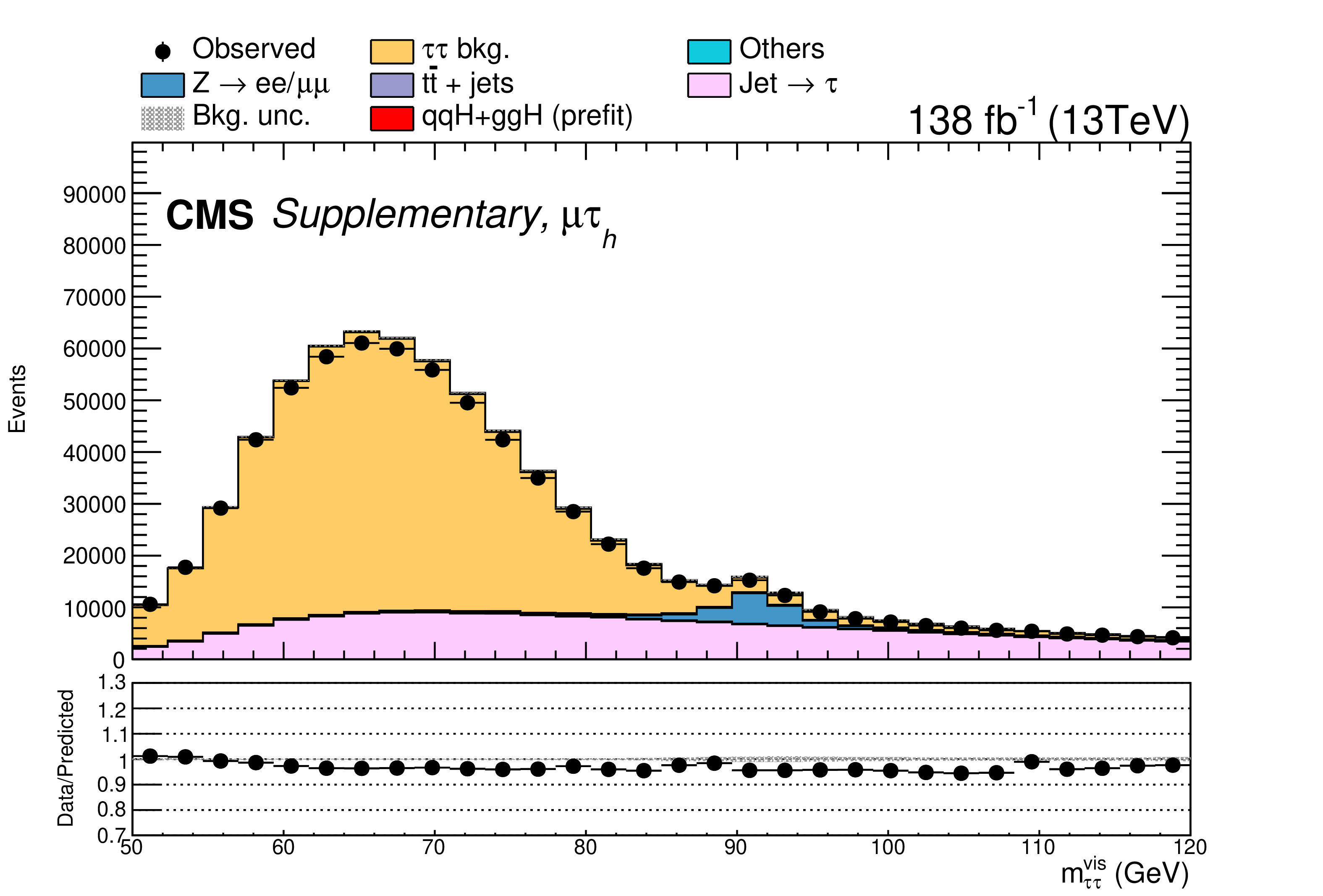
Additional Figure 66:
Pre-fit visible mass distribution from the $ \mu \tau _\mathrm{h} $ final state of the CB-analysis. Only statistical errors are shown. |

png pdf |
Additional Figure 67:
Pre-fit visible mass distribution from the $ \tau _\mathrm{h} \tau _\mathrm{h} $ final state of the CB-analysis. Only statistical errors are shown. |
| Additional Tables | |

png pdf |
Additional Table 1:
List of features used for training of the NNs in the $ \tau _\mathrm{h} \tau _\mathrm{h} $, $ \mathrm{e} \tau _\mathrm{h} $, $ \mu \tau _\mathrm{h} $, and $ \mathrm{e} \mu $ final states of the NN-analysis. First and second lepton refers to the label of the final state of each corresponding column, $ p_{\mathrm T}^{\text{jj}} $ refers to the vector sum of the $ p_{\mathrm{T}} $ of the two leading jets, and $ Q^{2}_{\mathrm{V}_{1(2)}} $ to the estimate of the momentum transfer of the first (second) exchanged vector boson under the VBF hypothesis, as described in the text of the paper. All other variables are also described in the text of the paper. |

png pdf |
Additional Table 2:
Observed and expected event yields after the fit of the background model to the data. The yields are shown split by the STXS stage-0 categories in the $ \mathrm{e} \mu $ final state of the NN-analysis. The relative fractions of the most important background processes with respect to the total expected background yield are also shown. The process labels are given as defined in Section 5 and summarized in Table 3 of the paper. Signal comprises the ggH and qqH categories. |

png pdf |
Additional Table 3:
Observed and expected event yields after the fit of the background model to the data. The yields are shown split by the STXS stage-0 categories in the $ \mathrm{e} \tau _\mathrm{h} $ final state of the NN-analysis. The relative fractions of the most important background processes with respect to the total expected background yield are also shown. The process labels are given as defined in Section 5 and summarized in Table 3 of the paper. Signal comprises the ggH and qqH categories. |

png pdf |
Additional Table 4:
Observed and expected event yields after the fit of the background model to the data. The yields are shown split by the STXS stage-0 categories in the $ \mu \tau _\mathrm{h} $ final state of the NN-analysis. The relative fractions of the most important background processes with respect to the total expected background yield are also shown. The process labels are given as defined in Section 5 and summarized in Table 3 of the paper. Signal comprises the ggH and qqH categories. |

png pdf |
Additional Table 5:
Observed and expected event yields after the fit of the background model to the data. The yields are shown split by the STXS stage-0 categories in the $ \tau _\mathrm{h} \tau _\mathrm{h} $ final state of the NN-analysis. The relative fractions of the most important background processes with respect to the total expected background yield are also shown. The process labels are given as defined in Section 5 and summarized in Table 3 of the paper. Signal comprises the ggH and qqH categories. |

png pdf |
Additional Table 6:
Observed and expected event yields after the fit of the background model to the data. The yields are shown split by the STXS stage-0 categories in the $ \mathrm{e} \mu $ final state of the NN-analysis, in the highest purity bin of each corresponding data-taking year. The relative fractions of the most important background processes with respect to the total expected background yield are also shown. The process labels are given as defined in Section 5 and summarized in Table 3 of the paper. Signal comprises the ggH and qqH categories. |

png pdf |
Additional Table 7:
Observed and expected event yields after the fit of the background model to the data. The yields are shown split by the STXS stage-0 categories in the $ \mathrm{e} \tau _\mathrm{h} $ final state of the NN-analysis, in the highest purity bin of each corresponding data-taking year. The relative fractions of the most important background processes with respect to the total expected background yield are also shown. The process labels are given as defined in Section 5 and summarized in Table 3 of the paper. Signal comprises the ggH and qqH categories. |

png pdf |
Additional Table 8:
Observed and expected event yields after the fit of the background model to the data. The yields are shown split by the STXS stage-0 categories in the $ \mu \tau _\mathrm{h} $ final state of the NN-analysis, in the highest purity bin of each corresponding data-taking year. The relative fractions of the most important background processes with respect to the total expected background yield are also shown. The process labels are given as defined in Section 5 and summarized in Table 3 of the paper. Signal comprises the ggH and qqH categories. |

png pdf |
Additional Table 9:
Observed and expected event yields after the fit of the background model to the data. The yields are shown split by the STXS stage-0 categories in the $ \tau _\mathrm{h} \tau _\mathrm{h} $ final state of the NN-analysis, in the highest purity bin of each corresponding data-taking year. The relative fractions of the most important background processes with respect to the total expected background yield are also shown. The process labels are given as defined in Section 5 and summarized in Table 3 of the paper. Signal comprises the ggH and qqH categories. |
| References | ||||
| 1 | S. L. Glashow | Partial-symmetries of weak interactions | NP 22 (1961) 579 | |
| 2 | S. Weinberg | A model of leptons | PRL 19 (1967) 1264 | |
| 3 | A. Salam | Weak and electromagnetic interactions | Conf. Proc. C 680519 (1968) 367 | |
| 4 | F. Englert and R. Brout | Broken symmetry and the mass of gauge vector mesons | PRL 13 (1964) 321 | |
| 5 | P. W. Higgs | Broken symmetries, massless particles and gauge fields | PL 12 (1964) 132 | |
| 6 | P. W. Higgs | Broken symmetries and the masses of gauge bosons | PRL 13 (1964) 508 | |
| 7 | G. S. Guralnik, C. R. Hagen, and T. W. B. Kibble | Global conservation laws and massless particles | PRL 13 (1964) 585 | |
| 8 | P. W. Higgs | Spontaneous symmetry breakdown without massless bosons | PR 145 (1966) 1156 | |
| 9 | T. W. B. Kibble | Symmetry breaking in non-abelian gauge theories | PR 155 (1967) 1554 | |
| 10 | ATLAS Collaboration | Observation of a new particle in the search for the standard model Higgs boson with the ATLAS detector at the LHC | PLB 716 (2012) 1 | 1207.7214 |
| 11 | CMS Collaboration | Observation of a new boson at a mass of 125 GeV with the CMS experiment at the LHC | PLB 716 (2012) 30 | CMS-HIG-12-028 1207.7235 |
| 12 | CMS Collaboration | Observation of a new boson with mass near 125 GeV in pp collisions at $\sqrt{s}$ = 7 and 8 TeV | JHEP 06 (2013) 081 | CMS-HIG-12-036 1303.4571 |
| 13 | CMS Collaboration | A measurement of the Higgs boson mass in the diphoton decay channel | PLB 805 (2020) 135425 | CMS-HIG-19-004 2002.06398 |
| 14 | CMS Collaboration | Measurement of the properties of a Higgs boson in the four-lepton final state | PRD 89 (2014) 092007 | CMS-HIG-13-002 1312.5353 |
| 15 | ATLAS and CMS Collaborations | Measurements of the Higgs boson production and decay rates and constraints on its couplings from a combined ATLAS and CMS analysis of the LHC pp collision data at $\sqrt{s}= $ 7 and 8 TeV | JHEP 08 (2016) 045 | 1606.02266 |
| 16 | CMS Collaboration | Combined measurements of Higgs boson couplings in proton-proton collisions at $\sqrt{s}= $ 13 TeV | EPJC 79 (2019) 421 | CMS-HIG-17-031 1809.10733 |
| 17 | ATLAS Collaboration | Combined measurements of Higgs boson production and decay using up to 80 fb$^{-1}$ of proton-proton collision data at $\sqrt{s}=$ 13 TeV collected with the ATLAS experiment | PRD 101 (2020) 012002 | 1909.02845 |
| 18 | ATLAS Collaboration | Higgs boson production cross-section measurements and their EFT interpretation in the 4 $ \ell $ decay channel at $\sqrt{s}=$13 TeV with the ATLAS detector | EPJC 80 (2020) 957 | 2004.03447 |
| 19 | CMS Collaboration | Measurements of the Higgs boson width and anomalous $ \mathrm{H} \mathrm{V} \mathrm{V} $ couplings from on-shell and off-shell production in the four-lepton final state | PRD 99 (2019) 112003 | CMS-HIG-18-002 1901.00174 |
| 20 | CMS Collaboration | Measurements of $\mathrm{t\bar{t}H}$ production and the CP structure of the Yukawa interaction between the Higgs boson and top quark in the diphoton decay channel | PRL 125 (2020) 061801 | CMS-HIG-19-013 2003.10866 |
| 21 | ATLAS Collaboration | CP properties of Higgs boson interactions with top quarks in the $\mathrm{t\bar{t}H}$ and $\mathrm{tH}$ processes using $\mathrm{H} \rightarrow \gamma\gamma$ with the ATLAS detector | PRL 125 (2020) 061802 | 2004.04545 |
| 22 | CMS Collaboration | Constraints on anomalous Higgs boson couplings to vector bosons and fermions in its production and decay using the four-lepton final state | PRD 104 (2021) 052004 | CMS-HIG-19-009 2104.12152 |
| 23 | ATLAS Collaboration | Constraints on Higgs boson properties using $WW^{*}(\rightarrow e\nu\mu\nu) jj$ production in 36.1 fb$^{-1}$ of $\sqrt{s}$=13 TeV pp collisions with the ATLAS detector | Submitted to Eur. Phys. J. C, 2021 | 2109.13808 |
| 24 | ATLAS Collaboration | Test of CP invariance in vector-boson fusion production of the Higgs boson in the $H\to \tau \tau $ channel in proton-proton collisions at $\sqrt{s}= $ 13 TeV with the ATLAS detector | PLB 805 (2020) 135426 | 2002.05315 |
| 25 | CMS Collaboration | Analysis of the $CP$ structure of the Yukawa coupling between the Higgs boson and $\tau$ leptons in proton-proton collisions at $\sqrt{s}$ = 13 TeV | JHEP 06 (2022) 012 | CMS-HIG-20-006 2110.04836 |
| 26 | Yu. A. Golfand and E. P. Likhtman | Extension of the algebra of Poincaré group generators and violation of p invariance | JETP Lett. 13 (1971) 323 | |
| 27 | J. Wess and B. Zumino | Supergauge transformations in four-dimensions | NPB 70 (1974) 39 | |
| 28 | ATLAS Collaboration | Search for additional heavy neutral Higgs and gauge bosons in the ditau final state produced in 36 fb$^{~1}$ of pp collisions at $\sqrt{s}= $ 13 TeV with the ATLAS detector | JHEP 01 (2018) 055 | 1709.07242 |
| 29 | CMS Collaboration | Search for additional neutral MSSM Higgs bosons in the $\tau\tau$ final state in proton-proton collisions at $\sqrt{s}=$ 13 TeV | JHEP 09 (2018) 007 | CMS-HIG-17-020 1803.06553 |
| 30 | CMS Collaboration | Evidence for the 125 GeV Higgs boson decaying to a pair of $\tau$ leptons | JHEP 05 (2014) 104 | CMS-HIG-13-004 1401.5041 |
| 31 | CMS Collaboration | Evidence for the direct decay of the 125 GeV Higgs boson to fermions | Nature Phys. 10 (2014) 557 | CMS-HIG-13-033 1401.6527 |
| 32 | ATLAS Collaboration | Evidence for the Higgs-boson Yukawa coupling to tau leptons with the ATLAS detector | JHEP 04 (2015) 117 | 1501.04943 |
| 33 | CMS Collaboration | Observation of the Higgs boson decay to a pair of $\tau$ leptons with the CMS detector | PLB 779 (2018) 283 | CMS-HIG-16-043 1708.00373 |
| 34 | LHC Higgs Cross Section Working Group | Handbook of LHC Higgs cross sections: 4. Deciphering the nature of the Higgs sector | CERN Report CERN-2017-002-M, 2016 link |
1610.07922 |
| 35 | N. Berger et al. | Simplified template cross sections - stage 1.1 | LHC Higgs Cross Section Working Group Report LHCHXSWG-2019-003, DESY-19-070, 2019 | 1906.02754 |
| 36 | ATLAS Collaboration | Cross-section measurements of the Higgs boson decaying into a pair of $\tau$-leptons in proton-proton collisions at $\sqrt{s}= $ 13 TeV with the ATLAS detector | PRD 99 (2019) 072001 | 1811.08856 |
| 37 | ATLAS Collaboration | Measurements of Higgs boson production cross-sections in the $H\to\tau^{+}\tau^{-}$ decay channel in pp collisions at $\sqrt{s}= $ 13 T with the ATLAS detector | Submitted to JHEP, 2022 | 2201.08269 |
| 38 | CMS Collaboration | Measurement of the inclusive and differential Higgs boson production cross sections in the decay mode to a pair of $\tau$ leptons in pp collisions at $\sqrt{s} = $ 13 TeV | PRL 128 (2022) 081805 | CMS-HIG-20-015 2107.11486 |
| 39 | CMS Collaboration | Performance of the CMS Level-1 trigger in proton-proton collisions at $\sqrt{s} = $ 13\,TeV | JINST 15 (2020) P10017 | CMS-TRG-17-001 2006.10165 |
| 40 | CMS Collaboration | The CMS trigger system | JINST 12 (2017) P01020 | CMS-TRG-12-001 1609.02366 |
| 41 | CMS Collaboration | The CMS experiment at the CERN LHC | JINST 3 (2008) S08004 | |
| 42 | CMS Collaboration | Particle-flow reconstruction and global event description with the CMS detector | JINST 12 (2017) P10003 | CMS-PRF-14-001 1706.04965 |
| 43 | CMS Collaboration | Technical proposal for the Phase-II upgrade of the Compact Muon Solenoid | CMS Technical Proposal CERN-LHCC-2015-010, CMS-TDR-15-02, 2015 CDS |
|
| 44 | CMS Collaboration | Performance of electron reconstruction and selection with the CMS detector in proton-proton collisions at $\sqrt{s} = $ 8 TeV | JINST 10 (2015) P06005 | CMS-EGM-13-001 1502.02701 |
| 45 | CMS Collaboration | Electron and photon reconstruction and identification with the CMS experiment at the CERN LHC | JINST 16 (2021) P05014 | CMS-EGM-17-001 2012.06888 |
| 46 | CMS Collaboration | Performance of CMS muon reconstruction in pp collision events at $\sqrt{s}= $ 7 TeV | JINST 7 (2012) P10002 | CMS-MUO-10-004 1206.4071 |
| 47 | CMS Collaboration | Performance of the CMS muon detector and muon reconstruction with proton-proton collisions at $\sqrt{s}=$ 13 TeV | JINST 13 (2018) P06015 | CMS-MUO-16-001 1804.04528 |
| 48 | M. Cacciari, G. P. Salam, and G. Soyez | The anti-$ k_{\mathrm{T}} $ jet clustering algorithm | JHEP 04 (2008) 063 | 0802.1189 |
| 49 | M. Cacciari, G. P. Salam, and G. Soyez | FastJet user manual | EPJC 72 (2012) 1896 | 1111.6097 |
| 50 | CMS Collaboration | Identification of heavy-flavour jets with the CMS detector in pp collisions at 13 TeV | JINST 13 (2018) P05011 | CMS-BTV-16-002 1712.07158 |
| 51 | E. Bols et al. | Jet flavour classification using DeepJet | JINST 15 (2020) P12012 | 2008.10519 |
| 52 | CMS Collaboration | Performance of the DeepJet b tagging algorithm using 41.9/fb of data from proton-proton collisions at 13 TeV with Phase 1 CMS detector | CMS Detector Performance Note CMS-DP-2018-058, CERN, 2018 CDS |
|
| 53 | CMS Collaboration | Performance of reconstruction and identification of $\tau$ leptons decaying to hadrons and $\nu_\tau$ in pp collisions at $\sqrt{s}=$ 13 TeV | JINST 13 (2018) P10005 | CMS-TAU-16-003 1809.02816 |
| 54 | CMS Collaboration | Identification of hadronic tau lepton decays using a deep neural network | JINST 17 (2022) P07023 | CMS-TAU-20-001 2201.08458 |
| 55 | CMS Collaboration | Performance of the CMS missing transverse momentum reconstruction in pp data at $\sqrt{s}$ = 8 TeV | JINST 10 (2015) P02006 | CMS-JME-13-003 1411.0511 |
| 56 | D. Bertolini, P. Harris, M. Low, and N. Tran | Pileup per particle identification | JHEP 10 (2014) 059 | 1407.6013 |
| 57 | CMS Collaboration | Performance of missing transverse momentum reconstruction in proton-proton collisions at $\sqrt{s} = $ 13\,TeV using the CMS detector | JINST 14 (2019) P07004 | CMS-JME-17-001 1903.06078 |
| 58 | L. Bianchini, J. Conway, E. K. Friis, and C. Veelken | Reconstruction of the Higgs mass in $H\to\tau\tau$ events by dynamical likelihood techniques | J. Phys. Conf. Ser. 513 (2014) 022035 | |
| 59 | B. K. Bullock, K. Hagiwara, and A. D. Martin | Tau polarization and its correlations as a probe of new physics | NPB 395 (1993) 499 | |
| 60 | Particle Data Group , P. A. Zyla et al. | Review of particle physics | Prog. Theor. Exp. Phys. 2020 (2020) 083C01 | |
| 61 | CMS Collaboration | Electron performance using first data collected by CMS in 2016 | CMS Detector Performance Note CMS-DP-2016-026, 2016 CDS |
|
| 62 | CMS Collaboration | Performance of muon reconstruction including alignment position errors for 2016 collision data | CMS Detector Performance Note CMS-DP-2016-067, 2016 CDS |
|
| 63 | CMS Collaboration | Tau lepton Run 2 trigger performance | CMS Detector Performance Note CMS-DP-2019-012, 2019 CDS |
|
| 64 | CMS Collaboration | An embedding technique to determine $\tau\tau$ backgrounds in proton-proton collision data | JINST 14 (2019) P06032 | CMS-TAU-18-001 1903.01216 |
| 65 | CMS Collaboration | Measurement of the $\mathrm{Z}\gamma^{*}\to\tau\tau$ cross section in pp collisions at $\sqrt{s}=$ 13 TeV and validation of $\tau$ lepton analysis techniques | EPJC 78 (2018) 708 | CMS-HIG-15-007 1801.03535 |
| 66 | J. Alwall et al. | MadGraph 5: Going beyond | JHEP 06 (2011) 128 | 1106.0522 |
| 67 | J. Alwall et al. | The automated computation of tree-level and next-to-leading order differential cross sections, and their matching to parton shower simulations | JHEP 07 (2014) 079 | 1405.0301 |
| 68 | J. Alwall et al. | Comparative study of various algorithms for the merging of parton showers and matrix elements in hadronic collisions | EPJC 53 (2008) 473 | 0706.2569 |
| 69 | P. Nason | A new method for combining NLO QCD with shower Monte Carlo algorithms | JHEP 11 (2004) 040 | hep-ph/0409146 |
| 70 | S. Frixione, P. Nason, and C. Oleari | Matching NLO QCD computations with parton shower simulations: the POWHEG method | JHEP 11 (2007) 070 | 0709.2092 |
| 71 | S. Alioli, P. Nason, C. Oleari, and E. Re | NLO Higgs boson production via gluon fusion matched with shower in POWHEG | JHEP 04 (2009) 002 | 0812.0578 |
| 72 | S. Alioli, P. Nason, C. Oleari, and E. Re | A general framework for implementing NLO calculations in shower Monte Carlo programs: the POWHEG BOX | JHEP 06 (2010) 043 | 1002.2581 |
| 73 | S. Alioli et al. | Jet pair production in POWHEG | JHEP 04 (2011) 081 | 1012.3380 |
| 74 | E. Bagnaschi, G. Degrassi, P. Slavich, and A. Vicini | Higgs production via gluon fusion in the POWHEG approach in the SM and in the MSSM | JHEP 02 (2012) 088 | 1111.2854 |
| 75 | P. Nason and C. Oleari | NLO Higgs boson production via vector-boson fusion matched with shower in POWHEG | JHEP 02 (2010) 037 | 0911.5299 |
| 76 | G. Luisoni, P. Nason, C. Oleari, and F. Tramontano | $ \mathrm{H} \mathrm{W}^{\pm} $/$ \mathrm{H} \mathrm{Z} $ + 0 and 1 jet at NLO with the POWHEG BOX interfaced to GoSam and their merging within MiNLO | JHEP 10 (2013) 083 | 1306.2542 |
| 77 | H. B. Hartanto, B. Jager, L. Reina, and D. Wackeroth | Higgs boson production in association with top quarks in the POWHEG BOX | PRD 91 (2015) 094003 | 1501.04498 |
| 78 | K. Hamilton, P. Nason, E. Re, and G. Zanderighi | NNLOPS simulation of Higgs boson production | JHEP 10 (2013) 222 | 1309.0017 |
| 79 | K. Hamilton, P. Nason, and G. Zanderighi | Finite quark-mass effects in the NNLOPS POWHEG+MiNLO Higgs generator | JHEP 05 (2015) 140 | 1501.04637 |
| 80 | LHC Higgs Cross Section Working Group | Handbook of LHC Higgs cross sections: 3. Higgs properties: Report of the LHC Higgs Cross Section Working Group | CERN Report CERN-2013-004, 2013 link |
1307.1347 |
| 81 | NNPDF Collaboration | Parton distributions for the LHC run II | JHEP 04 (2015) 040 | 1410.8849 |
| 82 | NNPDF Collaboration | Parton distributions from high-precision collider data | EPJC 77 (2017) 663 | 1706.00428 |
| 83 | T. Sjöstrand et al. | An introduction to PYTHIA 8.2 | Comput. Phys. Commun. 191 (2015) 159 | 1410.3012 |
| 84 | CMS Collaboration | Event generator tunes obtained from underlying event and multiparton scattering measurements | EPJC 76 (2016) 155 | CMS-GEN-14-001 1512.00815 |
| 85 | CMS Collaboration | Extraction and validation of a new set of CMS PYTHIA8 tunes from underlying-event measurements | EPJC 80 (2020) 4 | CMS-GEN-17-001 1903.12179 |
| 86 | K. Melnikov and F. Petriello | Electroweak gauge boson production at hadron colliders through $\mathcal{O}(\alpha_\text{s}^{2})$ | PRD 74 (2006) 114017 | hep-ph/0609070 |
| 87 | M. Czakon and A. Mitov | Top++: A program for the calculation of the top-pair cross-section at hadron colliders | Comput. Phys. Commun. 185 (2014) 2930 | 1112.5675 |
| 88 | N. Kidonakis | Top quark production | in Helmholtz International Summer School on Physics of Heavy Quarks and Hadrons, 2014 link |
1311.0283 |
| 89 | J. M. Campbell, R. K. Ellis, and C. Williams | Vector boson pair production at the LHC | JHEP 07 (2011) 018 | 1105.0020 |
| 90 | T. Gehrmann et al. | $ \mathrm{W^+} \mathrm{W^-} $ production at hadron colliders in next to next to leading order QCD | PRL 113 (2014) 212001 | 1408.5243 |
| 91 | S. Agostinelli et al. | GEANT4---a simulation toolkit | NIM A 506 (2003) 250 | |
| 92 | I. J. Goodfellow, Y. Bengio, and A. Courville | Deep Learning | MIT Press, Cambridge, MA, USA, 2016 link |
|
| 93 | A. V. Gritsan, R. Röntsch, M. Schulze, and M. Xiao | Constraining anomalous Higgs boson couplings to the heavy flavor fermions using matrix element techniques | PRD 94 (2016) 055023 | 1606.03107 |
| 94 | S. Wunsch, R. Friese, R. Wolf, and G. Quast | Identifying the relevant dependencies of the neural network response on characteristics of the input space | Comput. Softw. Big Sci. 2 (2018) 5 | 1803.08782 |
| 95 | X. Glorot and Y. Bengio | Understanding the difficulty of training deep feedforward neural networks | in Proceedings of the thirteenth international conference on artificial intelligence and statistics, 2010 link |
|
| 96 | R. Shimizu et al. | Balanced mini-batch training for imbalanced image data classification with neural network | in First International Conference on Artificial Intelligence for Industries (AI4I), 2018 link |
|
| 97 | D. P. Kingma and J. Ba | Adam: A method for stochastic optimization | 1412.6980 | |
| 98 | A. N. Tikhonov | Solution of incorrectly formulated problems and the regularization method | Soviet Math. Dokl. 4 (1963) 1035 | |
| 99 | S. Baker and R. D. Cousins | Clarification of the use of chi-square and likelihood functions in fits to histograms | NIM 221 (1984) 437 | |
| 100 | CDF Collaboration | Search for neutral MSSM Higgs bosons decaying to tau pairs in $ \mathrm{p} \overline{\mathrm{p}} $ collisions at $\sqrt{s} = $ 1.96 TeV | PRL 96 (2006) 011802 | hep-ex/0508051 |
| 101 | CMS Collaboration | Search for the associated production of the Higgs boson and a vector boson in proton-proton collisions at $\sqrt{s}=$ 13 TeV via Higgs boson decays to $\tau$ leptons | JHEP 06 (2019) 093 | CMS-HIG-18-007 1809.03590 |
| 102 | R. J. Barlow and C. Beeston | Fitting using finite Monte Carlo samples | Comput. Phys. Commun. 77 (1993) 219 | |
| 103 | CMS Collaboration | Measurements of inclusive $ \mathrm{W} $ and $ \mathrm{Z} $ cross sections in pp collisions at $\sqrt{s}= $ 7 TeV | JHEP 01 (2011) 080 | CMS-EWK-10-002 1012.2466 |
| 104 | CMS Collaboration | Jet energy scale and resolution in the CMS experiment in pp collisions at 8 TeV | JINST 12 (2017) P02014 | CMS-JME-13-004 1607.03663 |
| 105 | CMS Collaboration | Measurement of the differential cross section for top quark pair production in pp collisions at $\sqrt{s} = $ 8 TeV | EPJC 75 (2015) 542 | CMS-TOP-12-028 1505.04480 |
| 106 | CMS Collaboration | Precision luminosity measurement in proton-proton collisions at $\sqrt{s} =$ 13 TeV in 2015 and 2016 at CMS | EPJC 81 (2021) 800 | CMS-LUM-17-003 2104.01927 |
| 107 | CMS Collaboration | CMS luminosity measurement for the 2017 data-taking period at $\sqrt{s} = $ 13 TeV | CMS Physics Analysis Summary, 2018 CMS-PAS-LUM-17-004 |
CMS-PAS-LUM-17-004 |
| 108 | CMS Collaboration | CMS luminosity measurement for the 2018 data-taking period at $\sqrt{s} = $ 13 TeV | CMS Physics Analysis Summary, 2019 CMS-PAS-LUM-18-002 |
CMS-PAS-LUM-18-002 |
| 109 | J. Butterworth et al. | PDF4LHC recommendations for LHC Run II | JPG 43 (2016) 023001 | 1510.03865 |
| 110 | CMS Collaboration | HEPData record for this analysis | link | |
|
|
Compact Muon Solenoid LHC, CERN |
|

|

|

|

|

|