

Compact Muon Solenoid
LHC, CERN
| CMS-HIG-21-008 ; CERN-EP-2022-081 | ||
| Search for Higgs boson decay to a charm quark-antiquark pair in proton-proton collisions at $\sqrt{s} = $ 13 TeV | ||
| CMS Collaboration | ||
| 11 May 2022 | ||
| Phys. Rev. Lett. 131 (2023) 061801 | ||
| Abstract: A search for the standard model Higgs boson decaying to a charm quark-antiquark pair, H $\to \mathrm{c\bar{c}}$, produced in association with a leptonically decaying V (W or Z) boson is presented. The search is performed with proton-proton collisions at $\sqrt{s}=$ 13 TeV collected by the CMS experiment, corresponding to an integrated luminosity of 138 fb$^{-1}$. Novel charm jet identification and analysis methods using machine learning techniques are employed. The analysis is validated by searching for Z $\to \mathrm{c\bar{c}}$ in VZ events, leading to its first observation at a hadron collider with a significance of 5.7 standard deviations. The observed (expected) upper limit on $\sigma(\mathrm{VH}) \mathcal{B}( \mathrm{H \to c\bar{c}} )$ is 0.94 (0.50$^{+0.22}_{-0.15}$) pb at 95% confidence level (CL), corresponding to 14 (7.6$^{+3.4}_{-2.3}$) times the standard model prediction. For the Higgs-charm Yukawa coupling modifier, ${\kappa_{\mathrm{c}}} $, the observed (expected) 95% CL interval is 1.1 $< |{\kappa_{\mathrm{c}}} | < $ 5.5 ($|{\kappa_{\mathrm{c}}} | < $ 3.4), the most stringent constraint to date. | ||
| Links: e-print arXiv:2205.05550 [hep-ex] (PDF) ; CDS record ; inSPIRE record ; HepData record ; Physics Briefing ; CADI line (restricted) ; | ||
| Figures & Tables | Summary | Additional Figures & Tables | References | CMS Publications |
|---|
| Figures | |
png pdf |
Figure 1:
Performance of ParticleNet (blue lines) for identifying a $\mathrm{c} \mathrm{\bar{c}} $ pair for large-$R$ jets with $ {p_{\mathrm {T}}} >$ 300 GeV. The solid (dashed) line shows the efficiency to correctly identify H $\to \mathrm{c\bar{c}}$ vs. the efficiency of misidentifying quarks or gluons from the V+jets process (vs. H $\to \mathrm{b\bar{b}}$). The red crosses represent the three working points used in the merged-jet analysis. The performance of DeepAK15 (yellow lines) used in Ref. [31] is shown for comparison. |

png pdf |
Figure 2:
Distribution of events as a function of $S/B$ in the VZ(Z $\to \mathrm{c\bar{c}}$) (left) and VH(H $\to \mathrm{c\bar{c}}$) (right) searches, where $S$ and $B$ are the postfit signal and background yields, respectively, in each bin of the fitted ${m ({\mathrm{H} _{\text {cand}}} )}$ or BDT discriminant distributions. The bottom panel shows the ratio of data to the total background, with the uncertainty in background indicated by gray hatching. The red line represents background plus SM signal divided by background. |

png pdf |
Figure 2-a:
Distribution of events as a function of $S/B$ in the VZ(Z $\to \mathrm{c\bar{c}}$) search, where $S$ and $B$ are the postfit signal and background yields, respectively, in each bin of the fitted ${m ({\mathrm{H} _{\text {cand}}} )}$ or BDT discriminant distributions. The bottom panel shows the ratio of data to the total background, with the uncertainty in background indicated by gray hatching. The red line represents background plus SM signal divided by background. |
png pdf |
Figure 2-b:
Distribution of events as a function of $S/B$ in the VH(H $\to \mathrm{c\bar{c}}$) search, where $S$ and $B$ are the postfit signal and background yields, respectively, in each bin of the fitted ${m ({\mathrm{H} _{\text {cand}}} )}$ or BDT discriminant distributions. The bottom panel shows the ratio of data to the total background, with the uncertainty in background indicated by gray hatching. The red line represents background plus SM signal divided by background. |
png pdf |
Figure 3:
Combined ${m ({\mathrm{H} _{\text {cand}}} )}$ distribution in all channels of the merged-jet analysis. The fitted ${m ({\mathrm{H} _{\text {cand}}} )}$ distribution in each SR is weighted by $S/(S+B)$, where $S$ and $B$ are the postfit VH(H $\to \mathrm{c\bar{c}}$) signal and total background yields. The lower panel shows data (points) and the fitted VH(H $\to \mathrm{c\bar{c}}$) (red) and VZ(Z $\to \mathrm{c\bar{c}}$) (grey) distributions after subtracting all other processes. Error bars represent pre-subtraction statistical uncertainties in data, while the gray hatching indicates the total uncertainty in the signal and all background processes. |
png pdf |
Figure 4:
The 95% CL upper limits on ${\mu _{{{\mathrm{V} \mathrm{H} (\mathrm{H} \to \mathrm{c} \mathrm{\bar{c}})}}}}$. Green and yellow bands indicate the 68 and 95% intervals on the expected limits, respectively. The vertical red line indicates the SM value $ {\mu _{{{\mathrm{V} \mathrm{H} (\mathrm{H} \to \mathrm{c} \mathrm{\bar{c}})}}}} =$ 1. |
| Tables | |
png pdf |
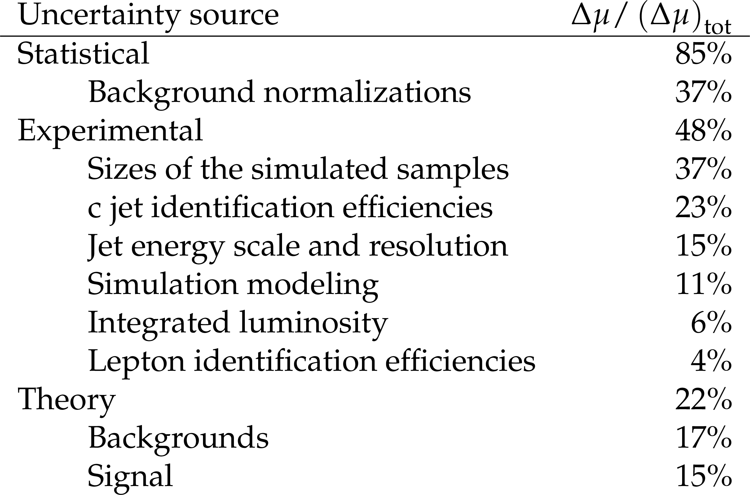
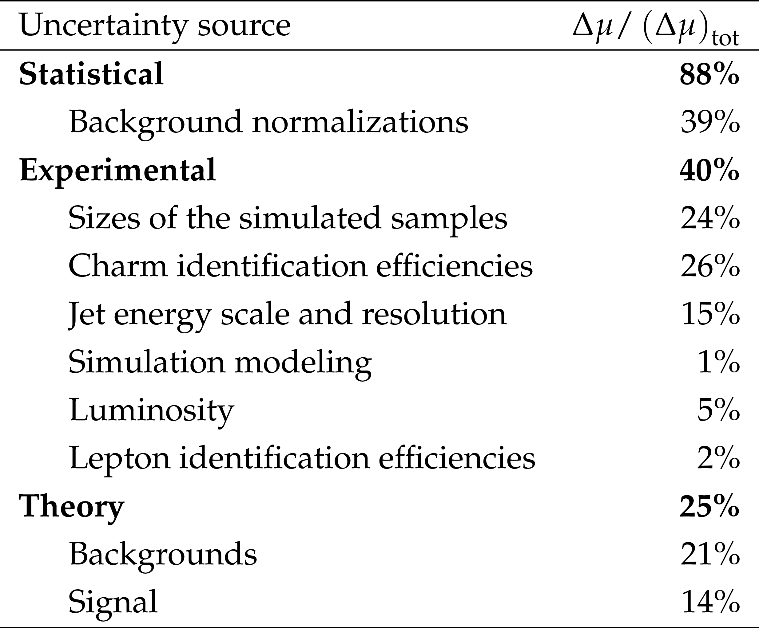
Table 1:
The relative contributions to the total uncertainty in the signal strength modifier $\mu $ for the VH(H $\to \mathrm{c\bar{c}}$) process, where the best fit is ${\mu _{{{\mathrm{V} \mathrm{H} (\mathrm{H} \to \mathrm{c} \mathrm{\bar{c}})}}}} = $ 7.7$^{+3.8}_{-3.5}$. |
| Summary |
| In summary, a search for the SM Higgs boson decaying to a pair of charm quarks in the CMS experiment is presented. Novel jet reconstruction and identification tools, and analysis techniques are developed for this analysis, which is validated by measuring the VZ(Z $\to \mathrm{c\bar{c}}$) process. The observed Z boson signal relative to the SM prediction is $\mu_{\mathrm{VZ(Z \to c\bar{c})}} =$ 1.01$_{-0.21}^{+0.23}$, with an observed (expected) significance of 5.7 (5.9) standard deviations above the background-only hypothesis. This is the first observation of Z $\to \mathrm{c\bar{c}}$ at a hadronic collider.The observed (expected) upper limit on $\sigma(\mathrm{VH}) \mathcal{B}( \mathrm{H \to c\bar{c}} )$ is 0.94 (0.50$^{+0.22}_{-0.15}$) pb, corresponding to 14 (7.6$^{+3.4}_{-2.3}$) times the theoretical prediction for an SM Higgs boson mass of 125.38 GeV. The observed (expected) 95% CL interval on the modifier, $\kappa_{\mathrm{c}}$, for the Yukawa coupling of the Higgs boson to the charm quark is 1.1 $< |{\kappa_{\mathrm{c}}}| < $ 5.5 ($|{\kappa_{\mathrm{c}}}| < $ 3.4). This is the most stringent constraint on $\kappa_{\mathrm{c}}$ to date. |
| Additional Figures | |
png pdf |
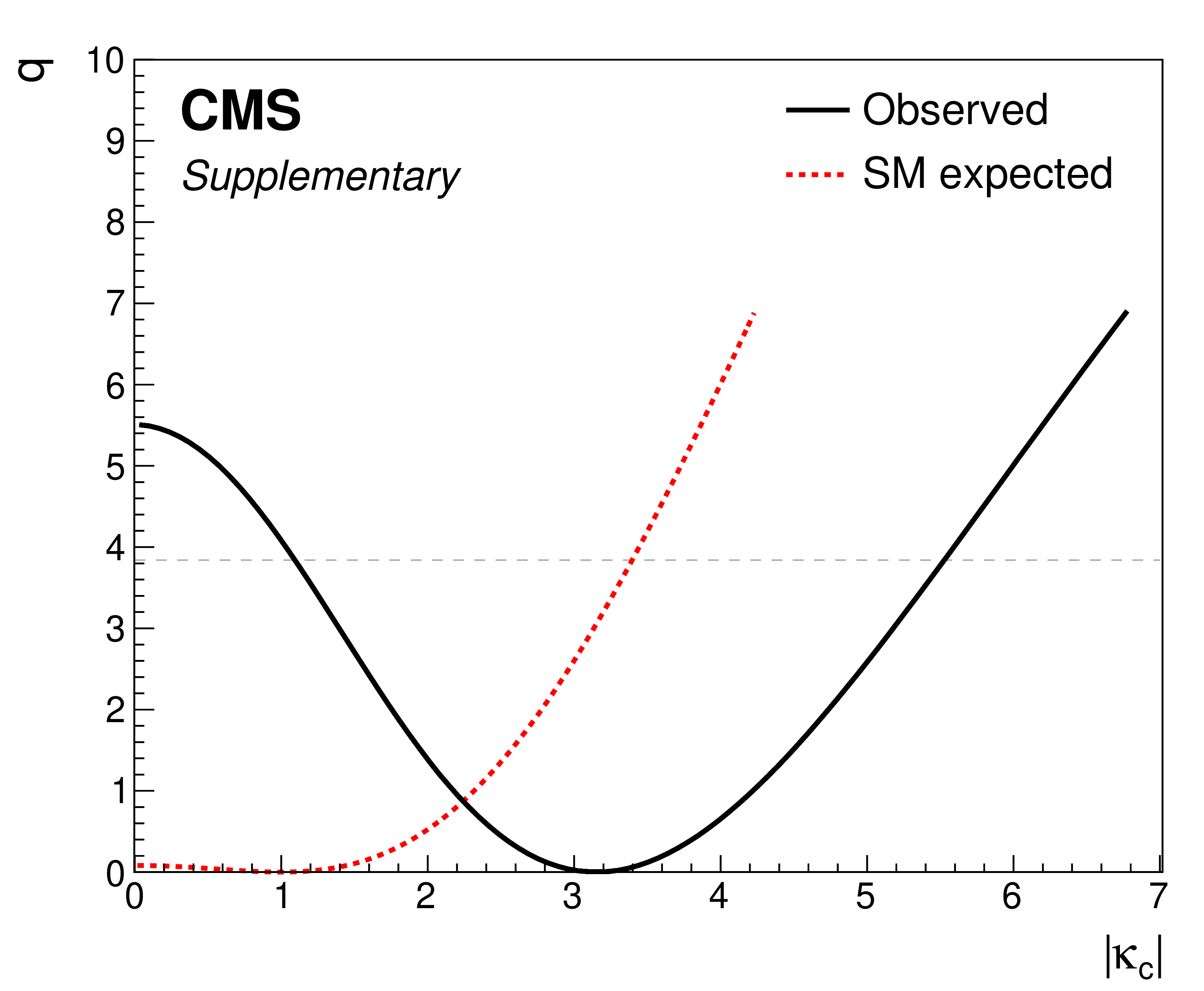
Additional Figure 1:
Scan of the test statistic $q$ as a function of $| {\kappa _{\mathrm{c}}} |$. Only the branching fraction $\mathcal{B}( \mathrm{ H \to c\bar{c} })$ is altered as ${\kappa _{\mathrm{c}}}$ varies, as described in the text. The expected SM result is also shown. The dashed horizontal line corresponds to the 95% confidence level. |

png pdf |
Additional Figure 2:
Best fit value of the VZ(Z $\to \mathrm{c\bar{c}}$) signal strength modifier ${\mu _{{{\mathrm{V} \mathrm{Z} (\mathrm{Z} \to \mathrm{c} \mathrm{\bar{c}})}}}}$ with its 1 and 2 standard deviation confidence intervals. The dashed vertical line indicates the SM value $ {\mu _{{{\mathrm{V} \mathrm{Z} (\mathrm{Z} \to \mathrm{c} \mathrm{\bar{c}})}}}} =$ 1. |
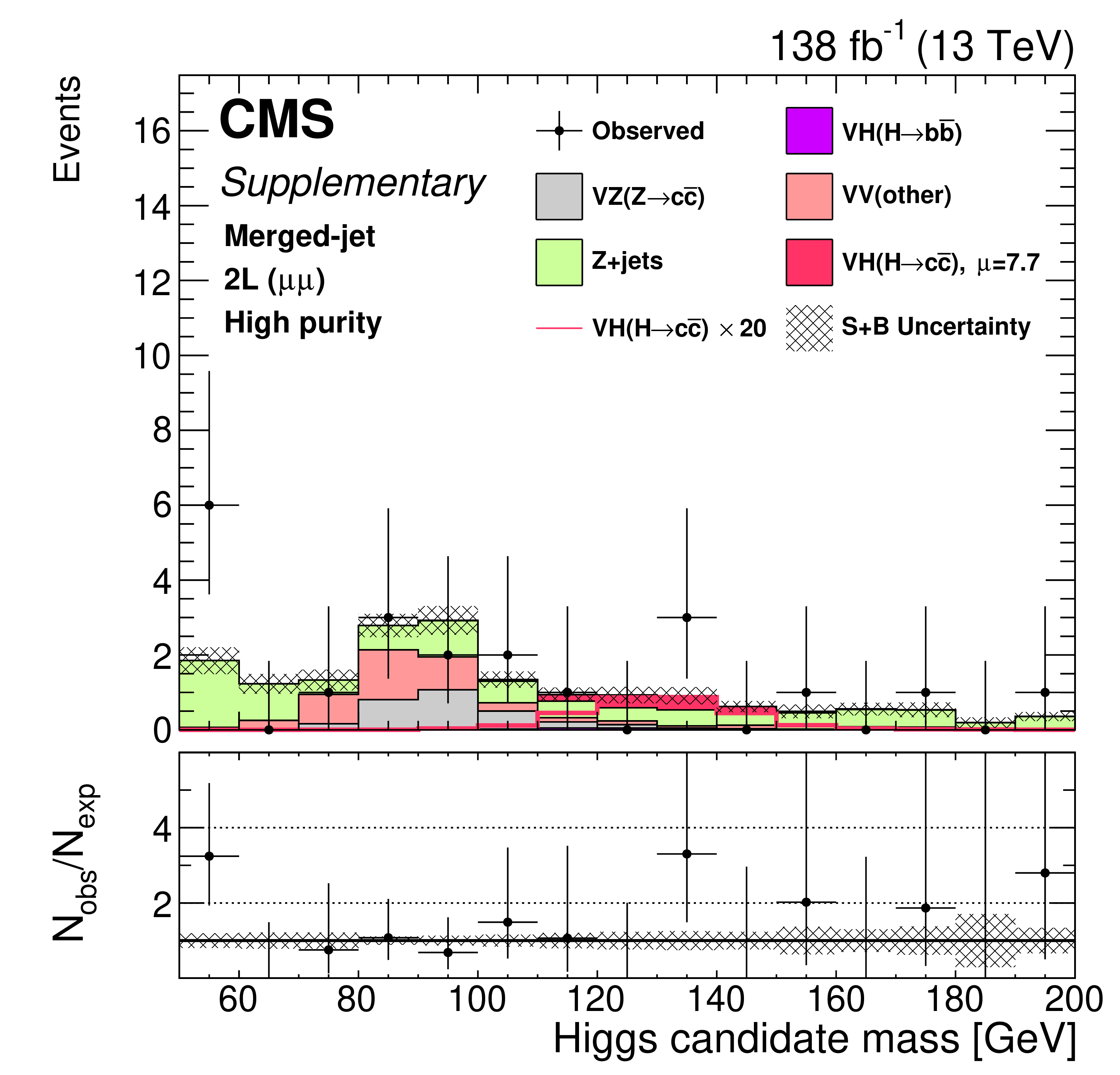
png pdf |
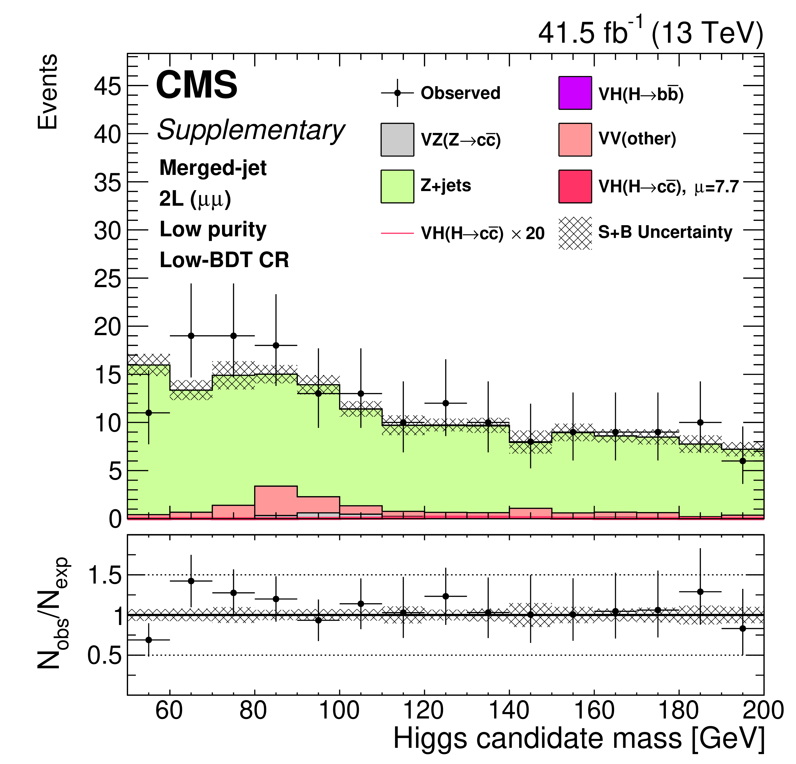
Additional Figure 3:
Post-fit distribution of ${m ({\mathrm{H} _{\text {cand}}} )}$ in the high-BDT and high $\mathrm{c} \mathrm{\bar{c}} $-purity signal region of the merged-jet topology in the 2L($\mu \mu $) channel. The VH(H $\to \mathrm{c\bar{c}}$) signal yield is scaled by the best fit signal strength, $ {\mu _{{{\mathrm{V} \mathrm{H} (\mathrm{H} \to \mathrm{c} \mathrm{\bar{c}})}}}} =$ 7.7, in the filled red histogram, and the red line represents the expected signal contribution multiplied by a factor of 20. |
png pdf |
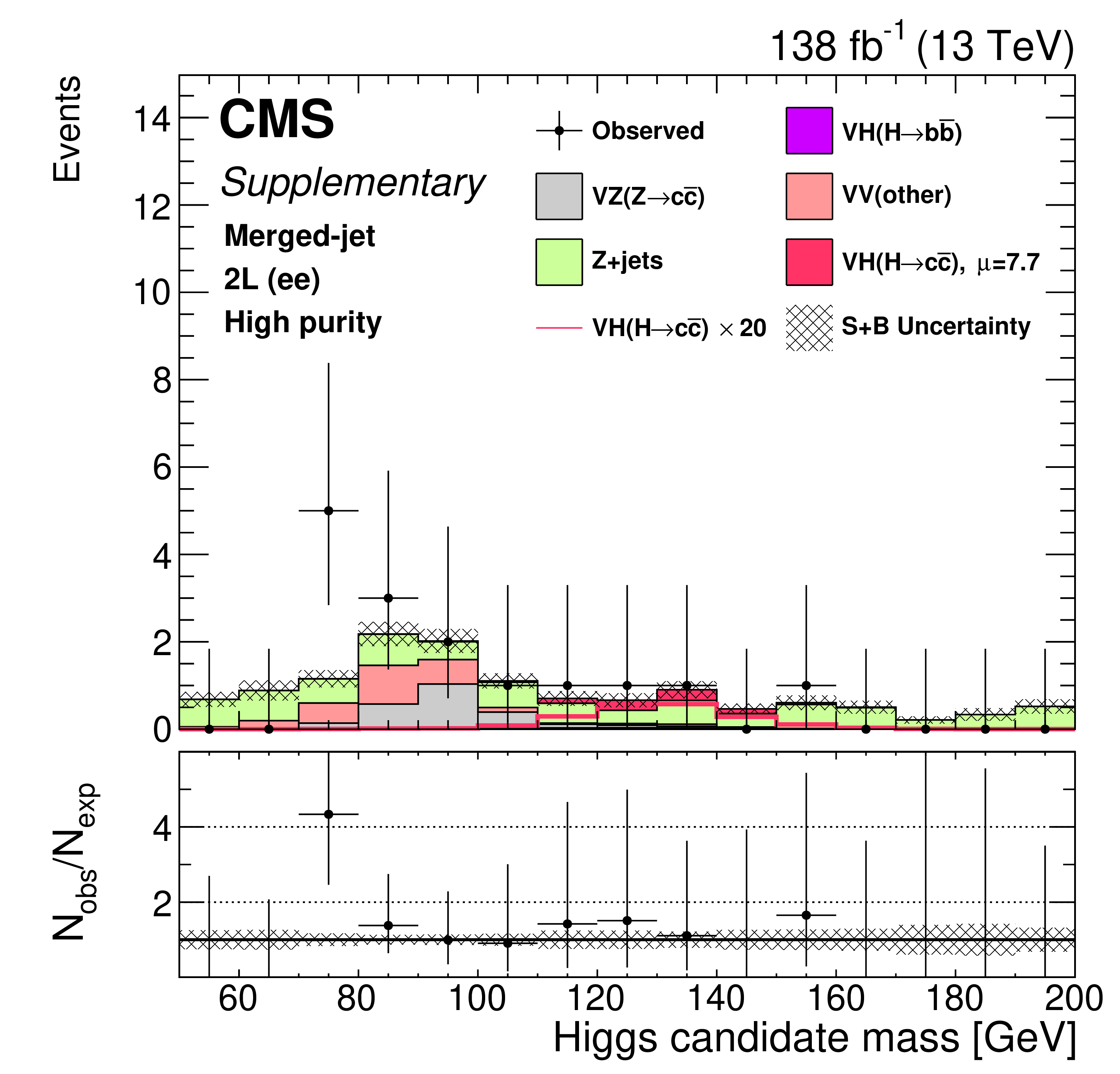
Additional Figure 4:
Post-fit distribution of ${m ({\mathrm{H} _{\text {cand}}} )}$ in the high-BDT and high $\mathrm{c} \mathrm{\bar{c}} $-purity signal region of the merged-jet topology in the 2L(ee) channel. The VH(H $\to \mathrm{c\bar{c}}$) signal yield is scaled by the best fit signal strength, $ {\mu _{{{\mathrm{V} \mathrm{H} (\mathrm{H} \to \mathrm{c} \mathrm{\bar{c}})}}}} =$ 7.7, in the filled red histogram, and the red line represents the expected signal contribution multiplied by a factor of 20. |

png pdf |
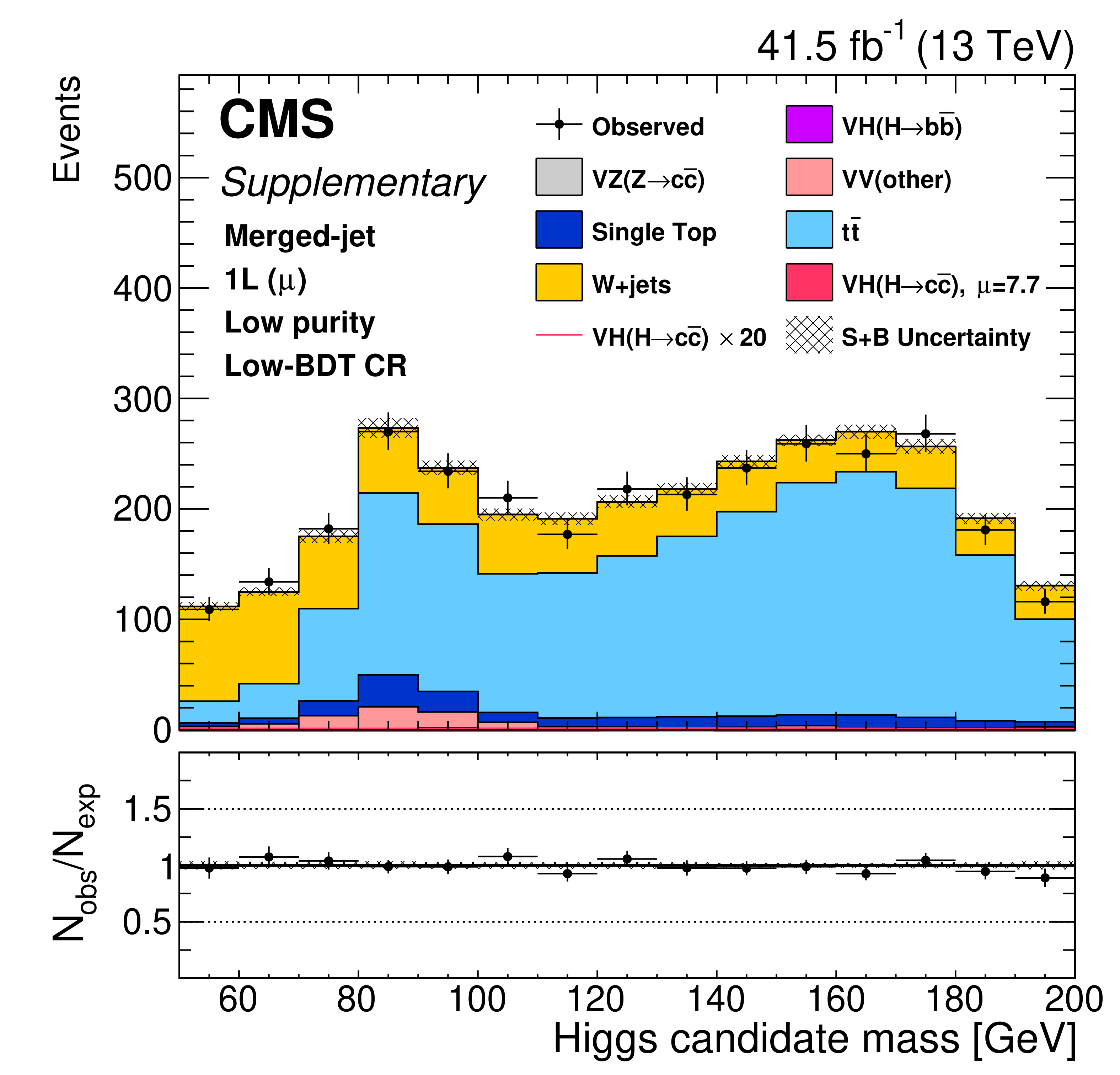
Additional Figure 5:
Post-fit distribution of ${m ({\mathrm{H} _{\text {cand}}} )}$ in the high-BDT and high $\mathrm{c} \mathrm{\bar{c}} $-purity signal region of the merged-jet topology in the 1L($\mu$) channel. The VH(H $\to \mathrm{c\bar{c}}$) signal yield is scaled by the best fit signal strength, $ {\mu _{{{\mathrm{V} \mathrm{H} (\mathrm{H} \to \mathrm{c} \mathrm{\bar{c}})}}}} =$ 7.7, in the filled red histogram, and the red line represents the expected signal contribution multiplied by a factor of 20. |
png pdf |
Additional Figure 6:
Post-fit distribution of ${m ({\mathrm{H} _{\text {cand}}} )}$ in the high-BDT and high $\mathrm{c} \mathrm{\bar{c}} $-purity signal region of the merged-jet topology in the 1L(e) channel. The VH(H $\to \mathrm{c\bar{c}}$) signal yield is scaled by the best fit signal strength, $ {\mu _{{{\mathrm{V} \mathrm{H} (\mathrm{H} \to \mathrm{c} \mathrm{\bar{c}})}}}} =$ 7.7, in the filled red histogram, and the red line represents the expected signal contribution multiplied by a factor of 20. |
png pdf |
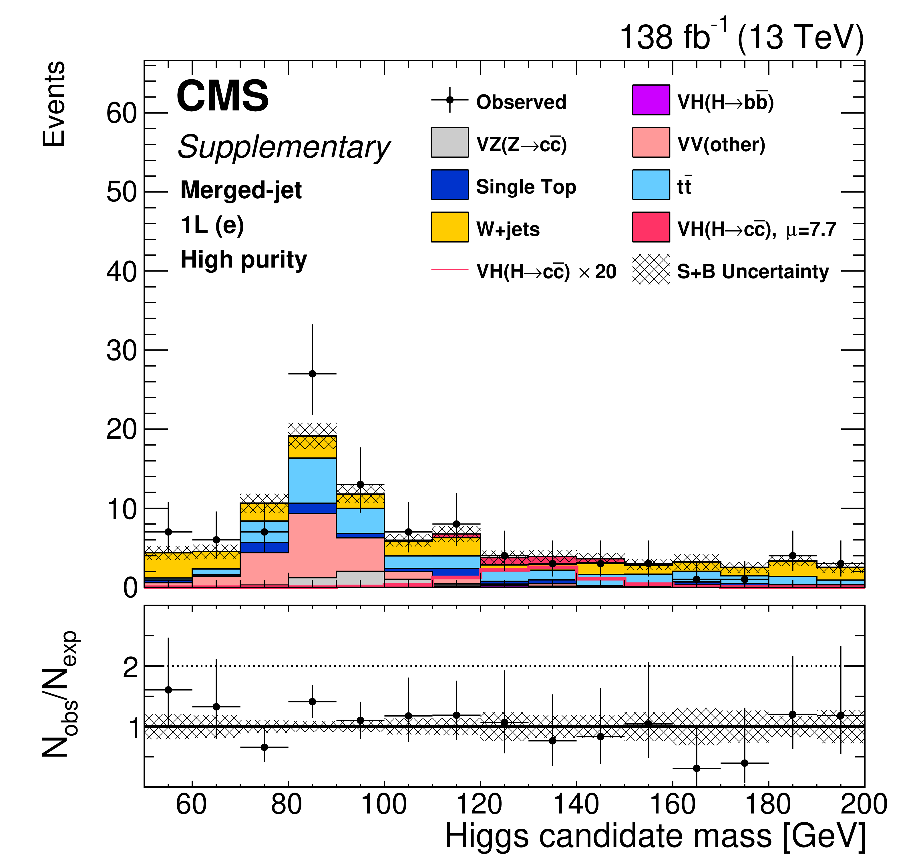
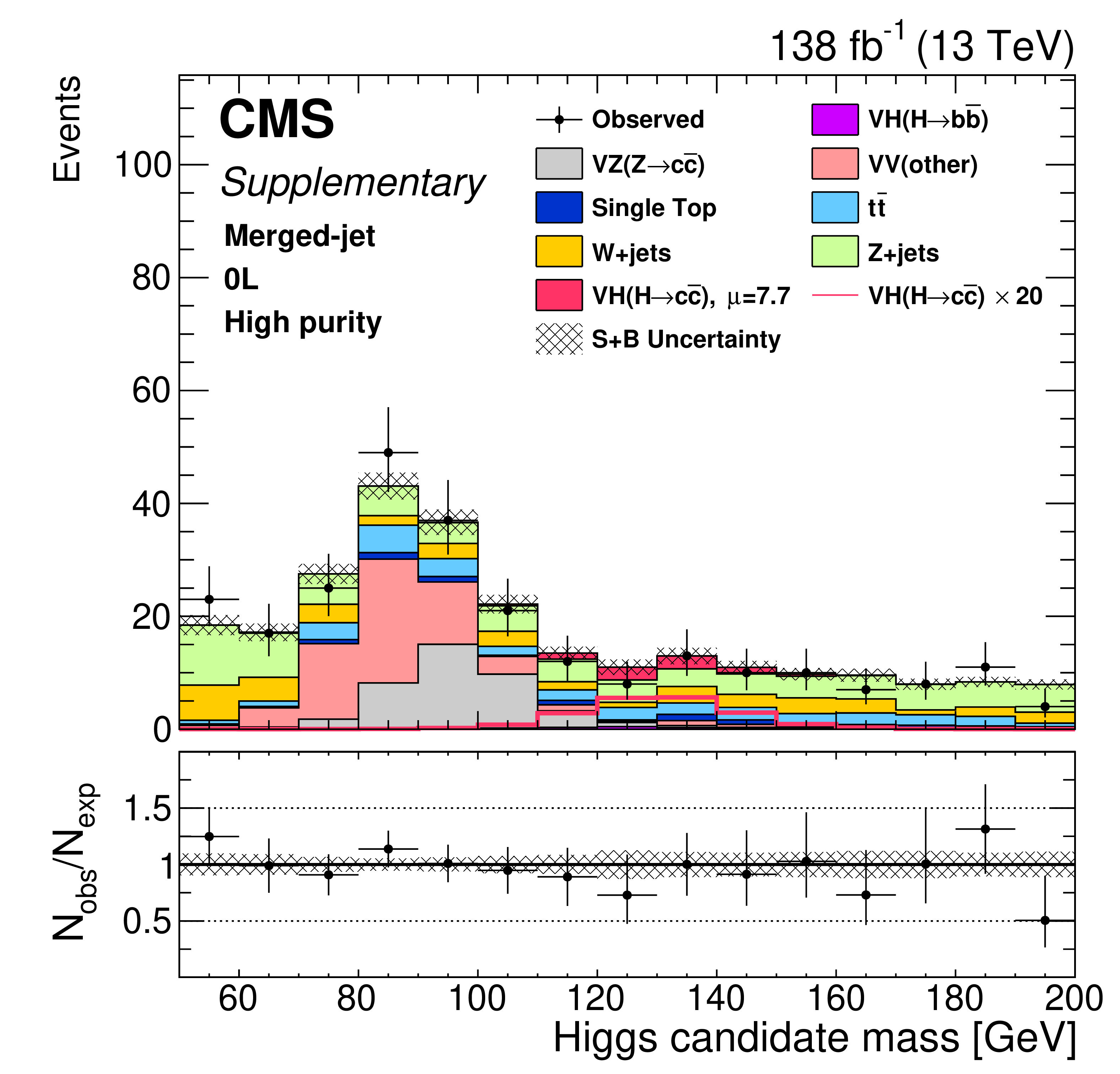
Additional Figure 7:
Post-fit distribution of ${m ({\mathrm{H} _{\text {cand}}} )}$ in the high-BDT and high $\mathrm{c} \mathrm{\bar{c}} $-purity signal region of the merged-jet topology in the 0L channel. The VH(H $\to \mathrm{c\bar{c}}$) signal yield is scaled by the best fit signal strength, $ {\mu _{{{\mathrm{V} \mathrm{H} (\mathrm{H} \to \mathrm{c} \mathrm{\bar{c}})}}}} =$ 7.7, in the filled red histogram, and the red line represents the expected signal contribution multiplied by a factor of 20. |
png pdf |
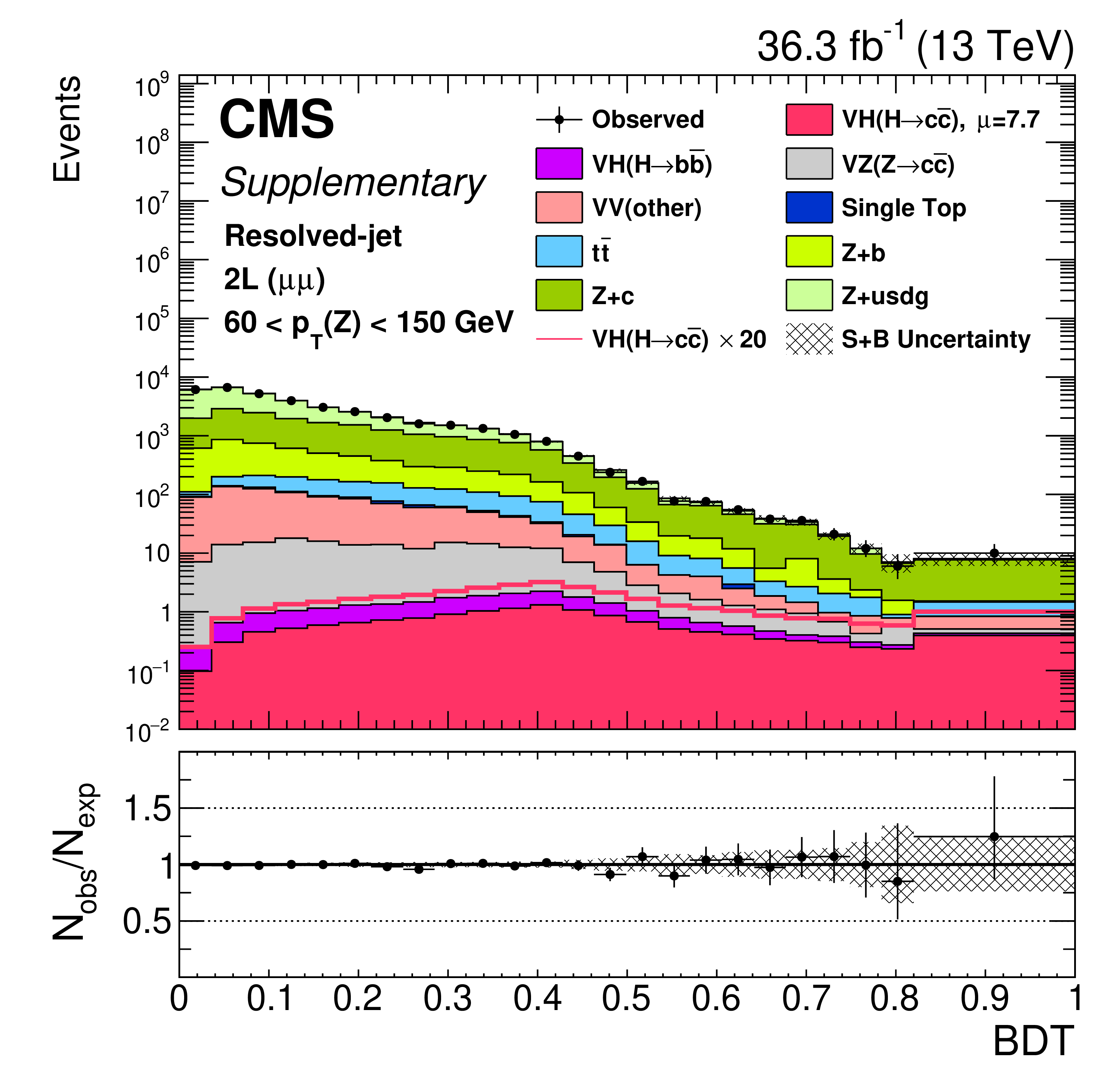
Additional Figure 8:
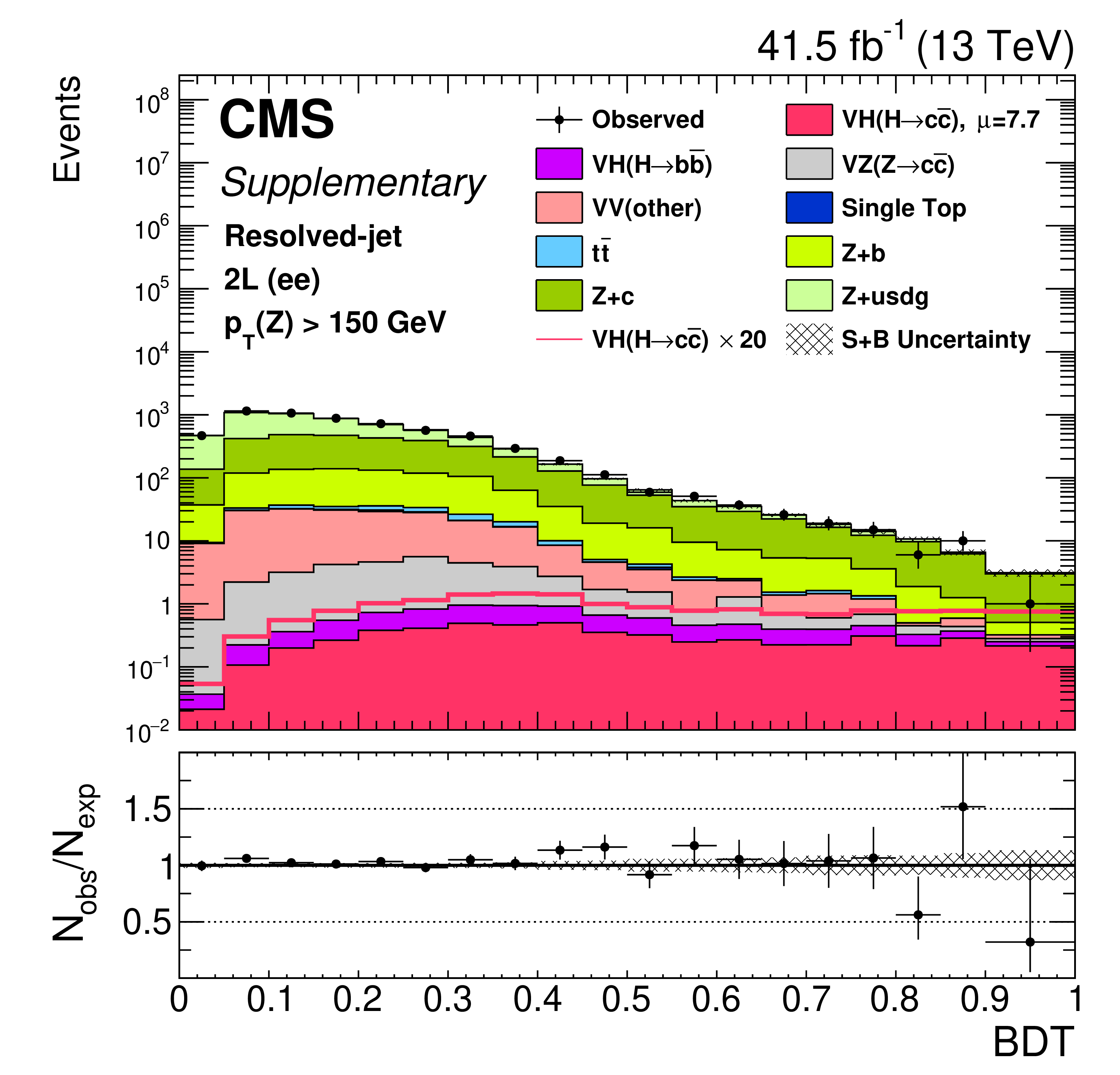
Post-fit distribution of the BDT discriminant in the low-$ {{p_{\mathrm {T}}} (\mathrm{V})}$ signal region of the resolved-jet topology in the 2L($\mu \mu $) channel in 2016 data. The VH(H $\to \mathrm{c\bar{c}}$) signal yield is scaled by the best fit signal strength, $ {\mu _{{{\mathrm{V} \mathrm{H} (\mathrm{H} \to \mathrm{c} \mathrm{\bar{c}})}}}} =$ 7.7, in the filled red histogram, and the red line represents the expected signal contribution multiplied by a factor of 20. |

png pdf |
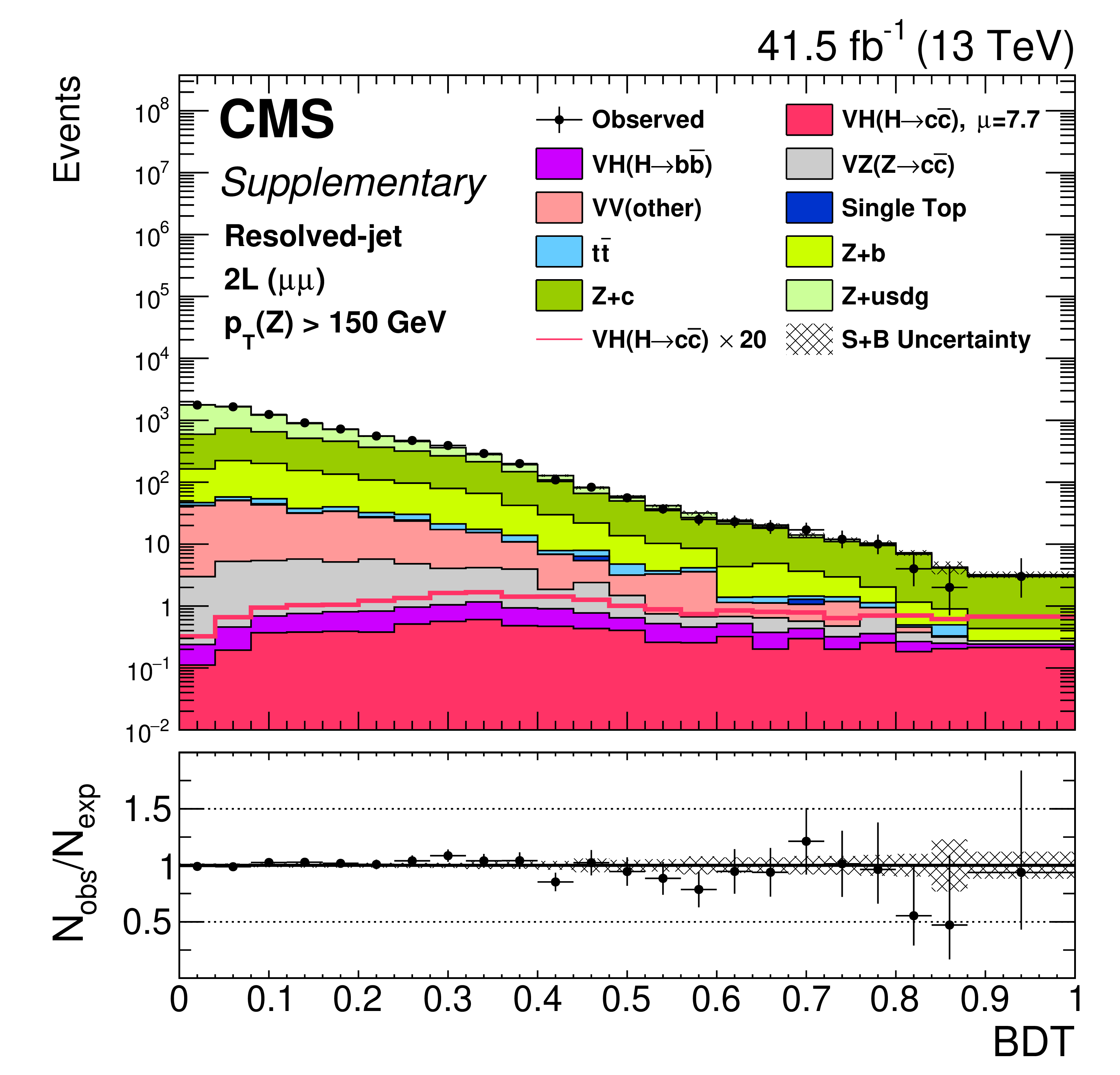
Additional Figure 9:
Post-fit distribution of the BDT discriminant in the low-$ {{p_{\mathrm {T}}} (\mathrm{V})}$ signal region of the resolved-jet topology in the 2L(ee) channel in 2016 data. The VH(H $\to \mathrm{c\bar{c}}$) signal yield is scaled by the best fit signal strength, $ {\mu _{{{\mathrm{V} \mathrm{H} (\mathrm{H} \to \mathrm{c} \mathrm{\bar{c}})}}}} =$ 7.7, in the filled red histogram, and the red line represents the expected signal contribution multiplied by a factor of 20. |
png pdf |
Additional Figure 10:
Post-fit distribution of the BDT discriminant in the high-$ {{p_{\mathrm {T}}} (\mathrm{V})}$ signal region of the resolved-jet topology in the 2L($\mu \mu $) channel in 2017 data. The VH(H $\to \mathrm{c\bar{c}}$) signal yield is scaled by the best fit signal strength, $ {\mu _{{{\mathrm{V} \mathrm{H} (\mathrm{H} \to \mathrm{c} \mathrm{\bar{c}})}}}} =$ 7.7, in the filled red histogram, and the red line represents the expected signal contribution multiplied by a factor of 20. |
png pdf |
Additional Figure 11:
Post-fit distribution of the BDT discriminant in the high-$ {{p_{\mathrm {T}}} (\mathrm{V})}$ signal region of the resolved-jet topology in the 2L(ee) channel in 2017 data. The VH(H $\to \mathrm{c\bar{c}}$) signal yield is scaled by the best fit signal strength, $ {\mu _{{{\mathrm{V} \mathrm{H} (\mathrm{H} \to \mathrm{c} \mathrm{\bar{c}})}}}} =$ 7.7, in the filled red histogram, and the red line represents the expected signal contribution multiplied by a factor of 20. |
png pdf |
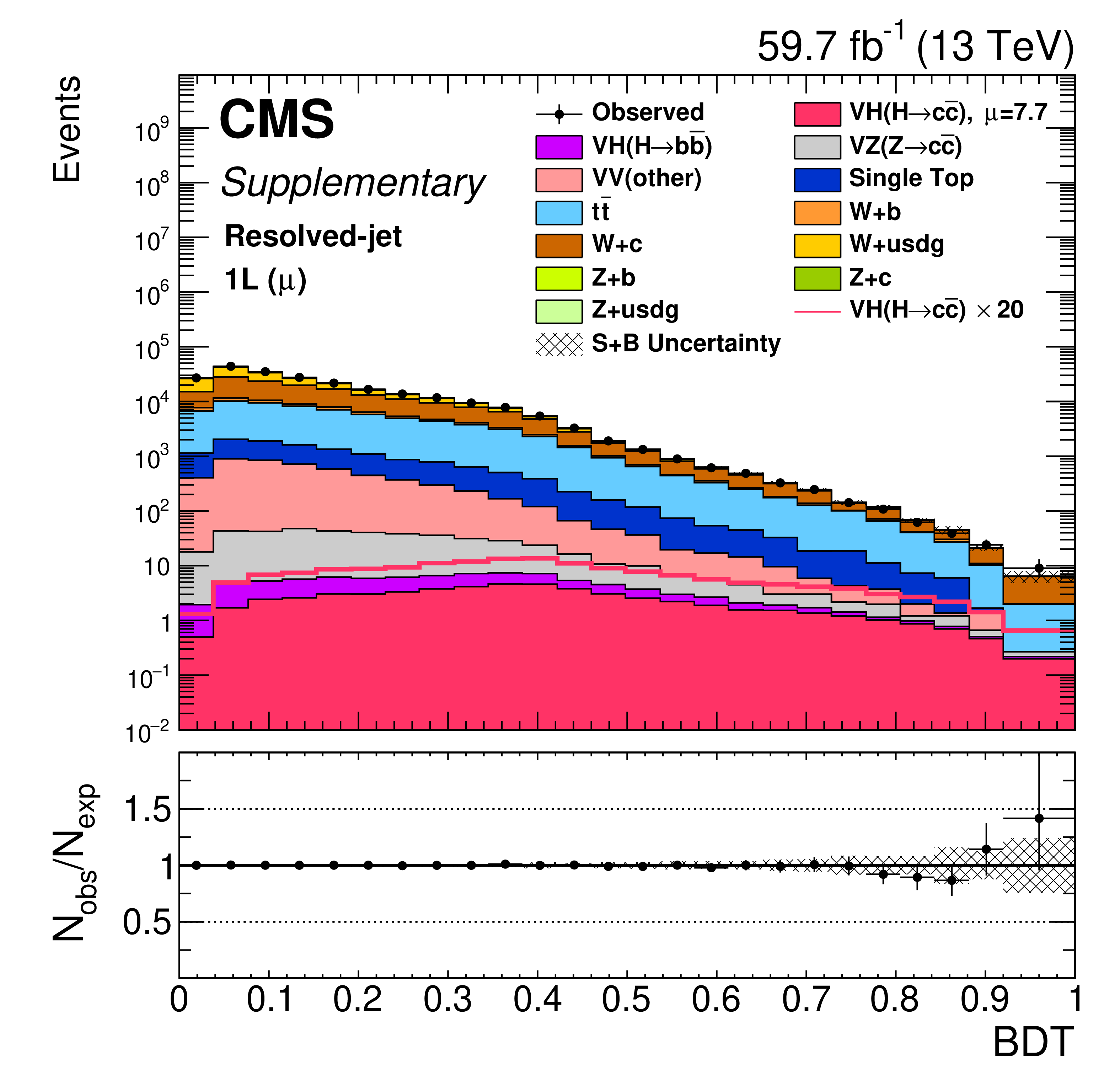
Additional Figure 12:
Post-fit distribution of the BDT discriminant in the signal region of the resolved-jet topology in the 1L($\mu$) channel in 2018 data. The VH(H $\to \mathrm{c\bar{c}}$) signal yield is scaled by the best fit signal strength, $ {\mu _{{{\mathrm{V} \mathrm{H} (\mathrm{H} \to \mathrm{c} \mathrm{\bar{c}})}}}} =$ 7.7, in the filled red histogram, and the red line represents the expected signal contribution multiplied by a factor of 20. |
png pdf |
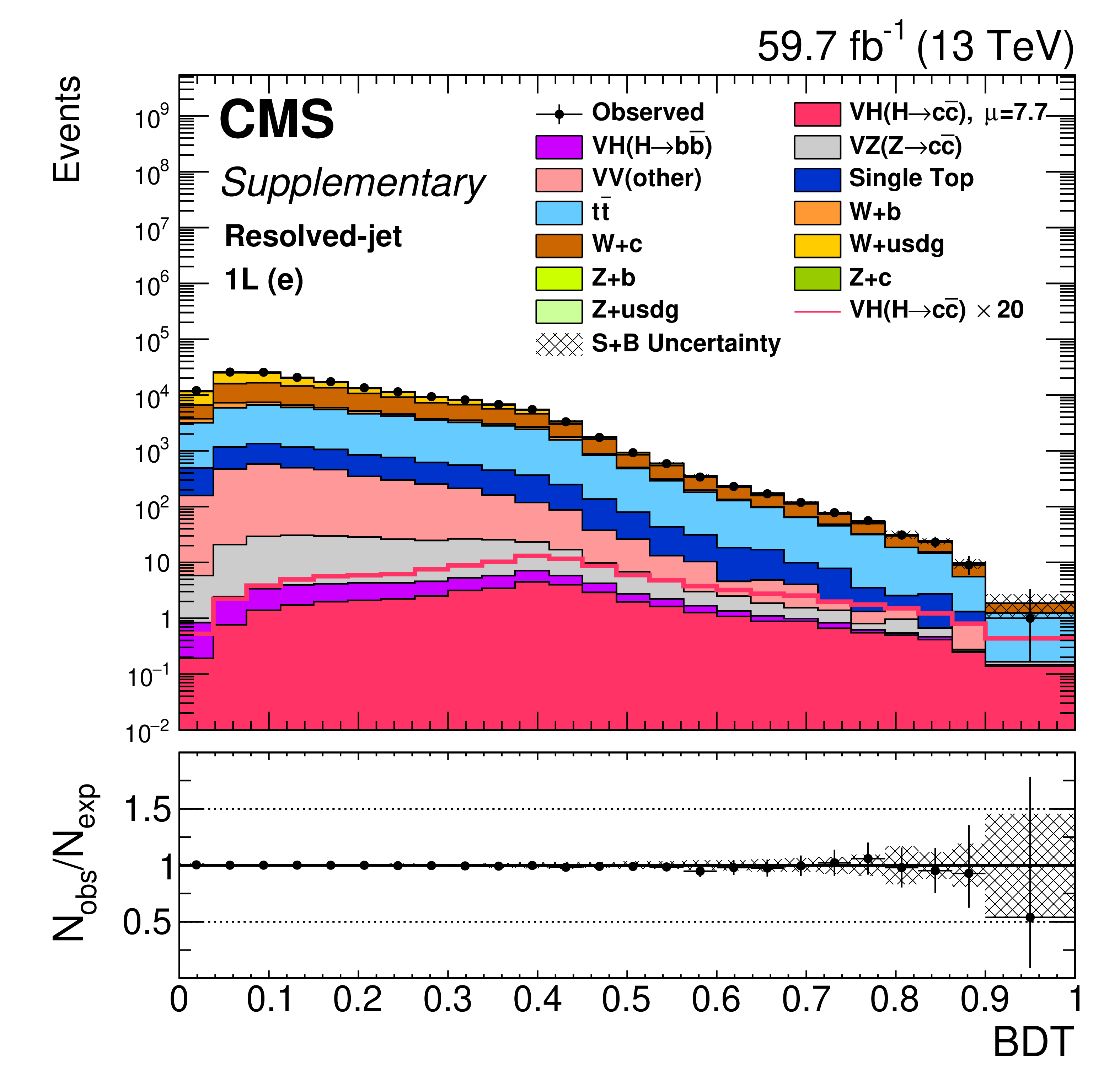
Additional Figure 13:
Post-fit distribution of the BDT discriminant in the signal region of the resolved-jet topology in the 1L(e) channel in 2018 data. The VH(H $\to \mathrm{c\bar{c}}$) signal yield is scaled by the best fit signal strength, $ {\mu _{{{\mathrm{V} \mathrm{H} (\mathrm{H} \to \mathrm{c} \mathrm{\bar{c}})}}}} =$ 7.7, in the filled red histogram, and the red line represents the expected signal contribution multiplied by a factor of 20. |
png pdf |
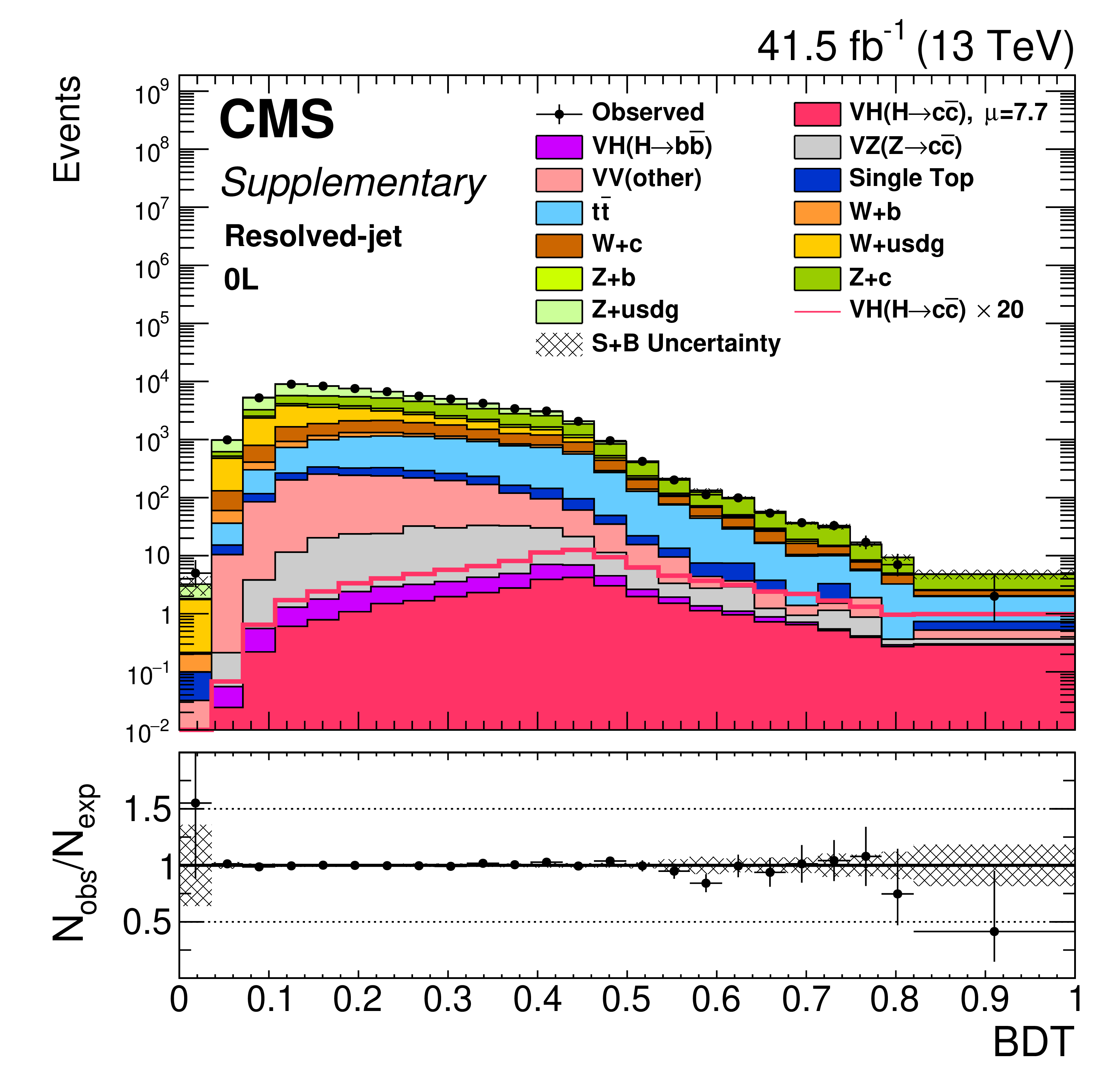
Additional Figure 14:
Post-fit distribution of the BDT discriminant in the signal region of the resolved-jet topology in the 0L channel in 2017 data. The VH(H $\to \mathrm{c\bar{c}}$) signal yield is scaled by the best fit signal strength, $ {\mu _{{{\mathrm{V} \mathrm{H} (\mathrm{H} \to \mathrm{c} \mathrm{\bar{c}})}}}} =$ 7.7, in the filled red histogram, and the red line represents the expected signal contribution multiplied by a factor of 20. |
png pdf |
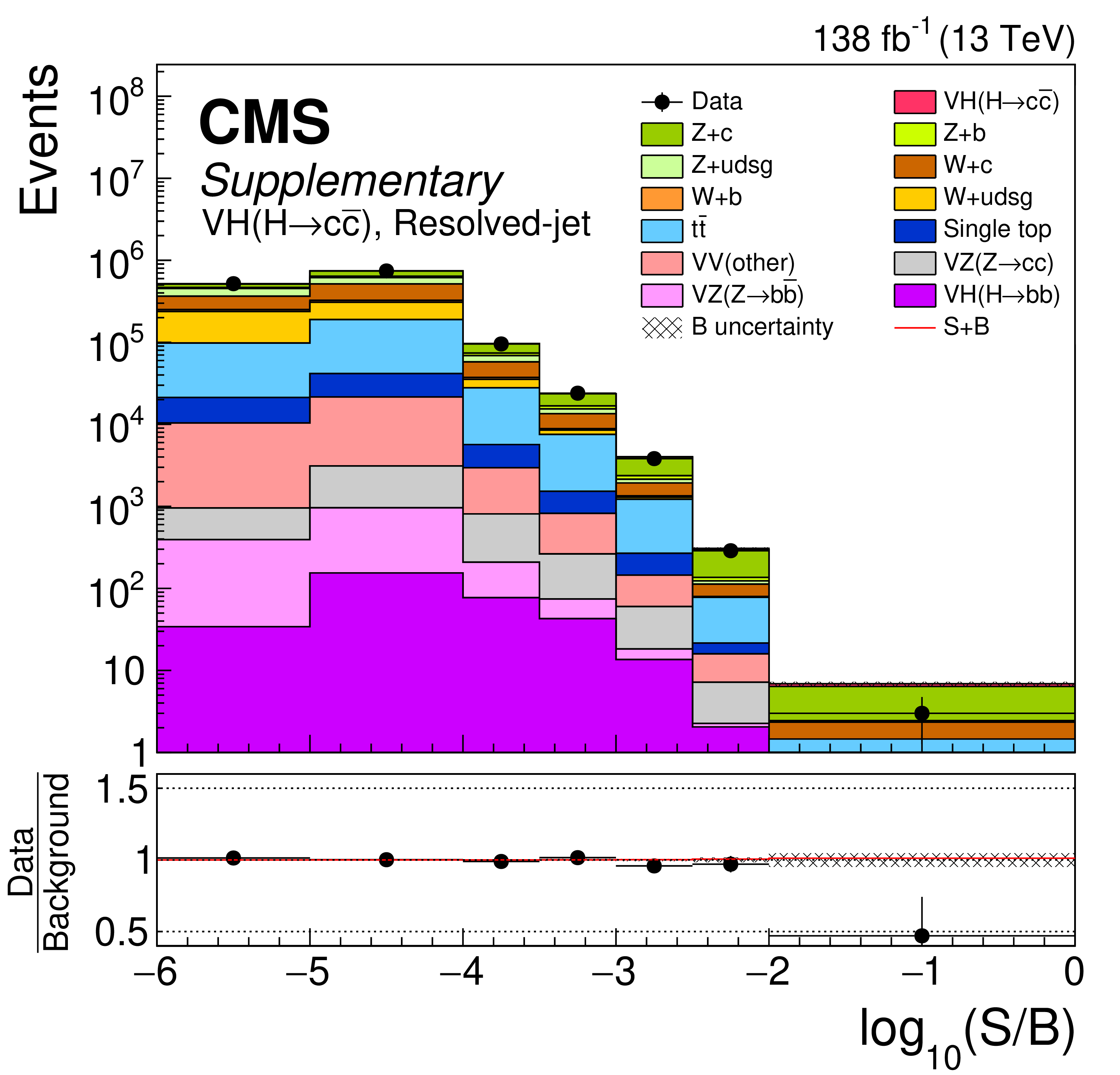
Additional Figure 15:
Distribution of events as a function of $S/B$ in the resolved-jet topology of the VH(H $\to \mathrm{c\bar{c}}$) search, where $S$ and $B$ are the postfit signal and background yields, respectively, in each bin of the fitted BDT discriminant distributions. The bottom panel shows the ratio of data to the total background, with the uncertainty in background indicated by gray hatching. The red line represents background plus SM signal divided by background. |
png pdf |
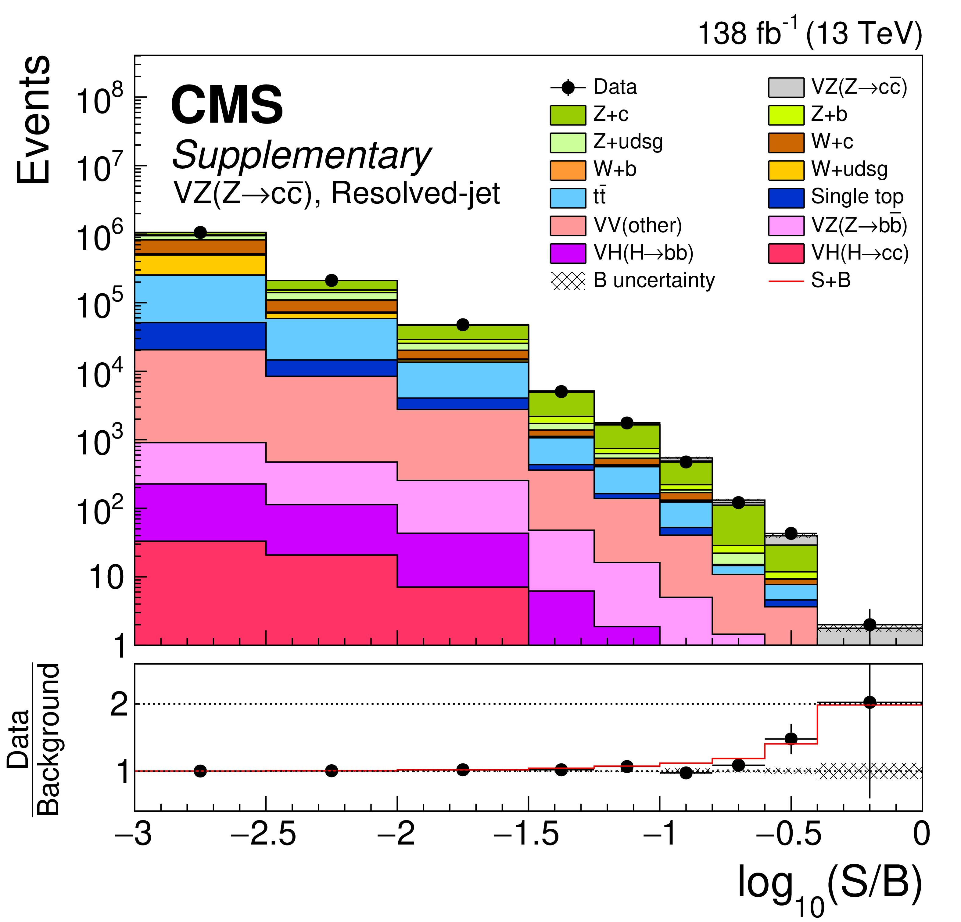
Additional Figure 16:
Distribution of events as a function of $S/B$ in the resolved-jet topology of the VZ(Z $\to \mathrm{c\bar{c}}$) search, where $S$ and $B$ are the postfit signal and background yields, respectively, in each bin of the fitted BDT discriminant distributions. The bottom panel shows the ratio of data to the total background, with the uncertainty in background indicated by gray hatching. The red line represents background plus SM signal divided by background. |
png pdf |
Additional Figure 17:
Post-fit distribution of ${m ({\mathrm{H} _{\text {cand}}} )}$ in the low-BDT and low $\mathrm{c} \mathrm{\bar{c}} $-purity control region of the merged-jet topology in the 2L($\mu \mu $) channel in 2017 data. The VH(H $\to \mathrm{c\bar{c}}$) signal yield is scaled by the best fit signal strength, $ {\mu _{{{\mathrm{V} \mathrm{H} (\mathrm{H} \to \mathrm{c} \mathrm{\bar{c}})}}}} =$ 7.7, in the filled red histogram, and the red line represents the expected signal contribution multiplied by a factor of 20. |

png pdf |
Additional Figure 18:
Post-fit distribution of ${m ({\mathrm{H} _{\text {cand}}} )}$ in the low-BDT and low $\mathrm{c} \mathrm{\bar{c}} $-purity control region of the merged-jet topology in the 2L(ee) channel in 2017 data. The VH(H $\to \mathrm{c\bar{c}}$) signal yield is scaled by the best fit signal strength, $ {\mu _{{{\mathrm{V} \mathrm{H} (\mathrm{H} \to \mathrm{c} \mathrm{\bar{c}})}}}} =$ 7.7, in the filled red histogram, and the red line represents the expected signal contribution multiplied by a factor of 20. |
png pdf |
Additional Figure 19:
Post-fit distribution of ${m ({\mathrm{H} _{\text {cand}}} )}$ in the low-BDT and low $\mathrm{c} \mathrm{\bar{c}} $-purity control region of the merged-jet topology in the 1L($\mu $) channel in 2017 data. The VH(H $\to \mathrm{c\bar{c}}$) signal yield is scaled by the best fit signal strength, $ {\mu _{{{\mathrm{V} \mathrm{H} (\mathrm{H} \to \mathrm{c} \mathrm{\bar{c}})}}}} =$ 7.7, in the filled red histogram, and the red line represents the expected signal contribution multiplied by a factor of 20. |
png pdf |
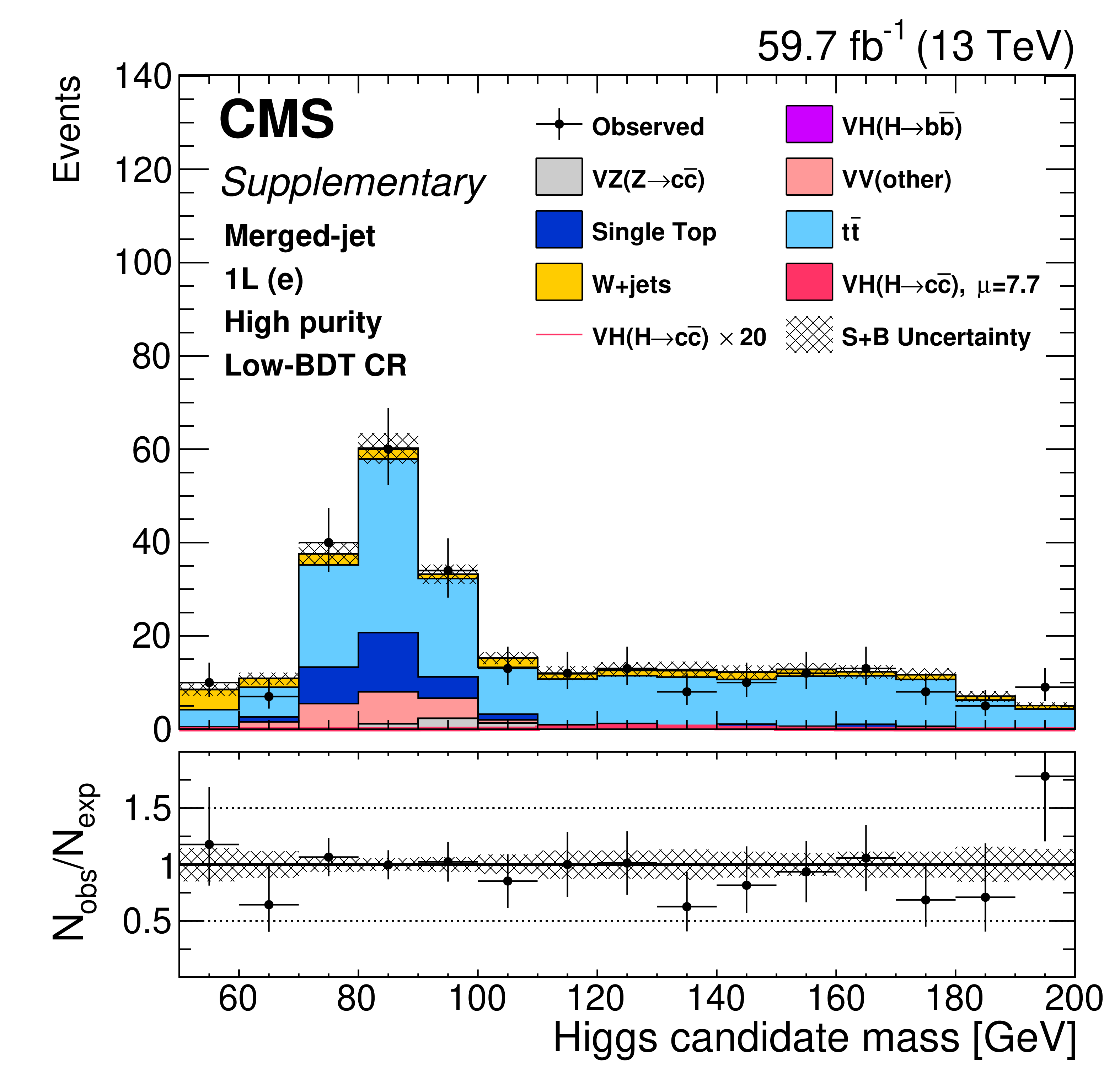
Additional Figure 20:
Post-fit distribution of ${m ({\mathrm{H} _{\text {cand}}} )}$ in the low-BDT and high $\mathrm{c} \mathrm{\bar{c}} $-purity control region of the merged-jet topology in the 1L(e) channel in 2018 data. The VH(H $\to \mathrm{c\bar{c}}$) signal yield is scaled by the best fit signal strength, $ {\mu _{{{\mathrm{V} \mathrm{H} (\mathrm{H} \to \mathrm{c} \mathrm{\bar{c}})}}}} =$ 7.7, in the filled red histogram, and the red line represents the expected signal contribution multiplied by a factor of 20. |
png pdf |
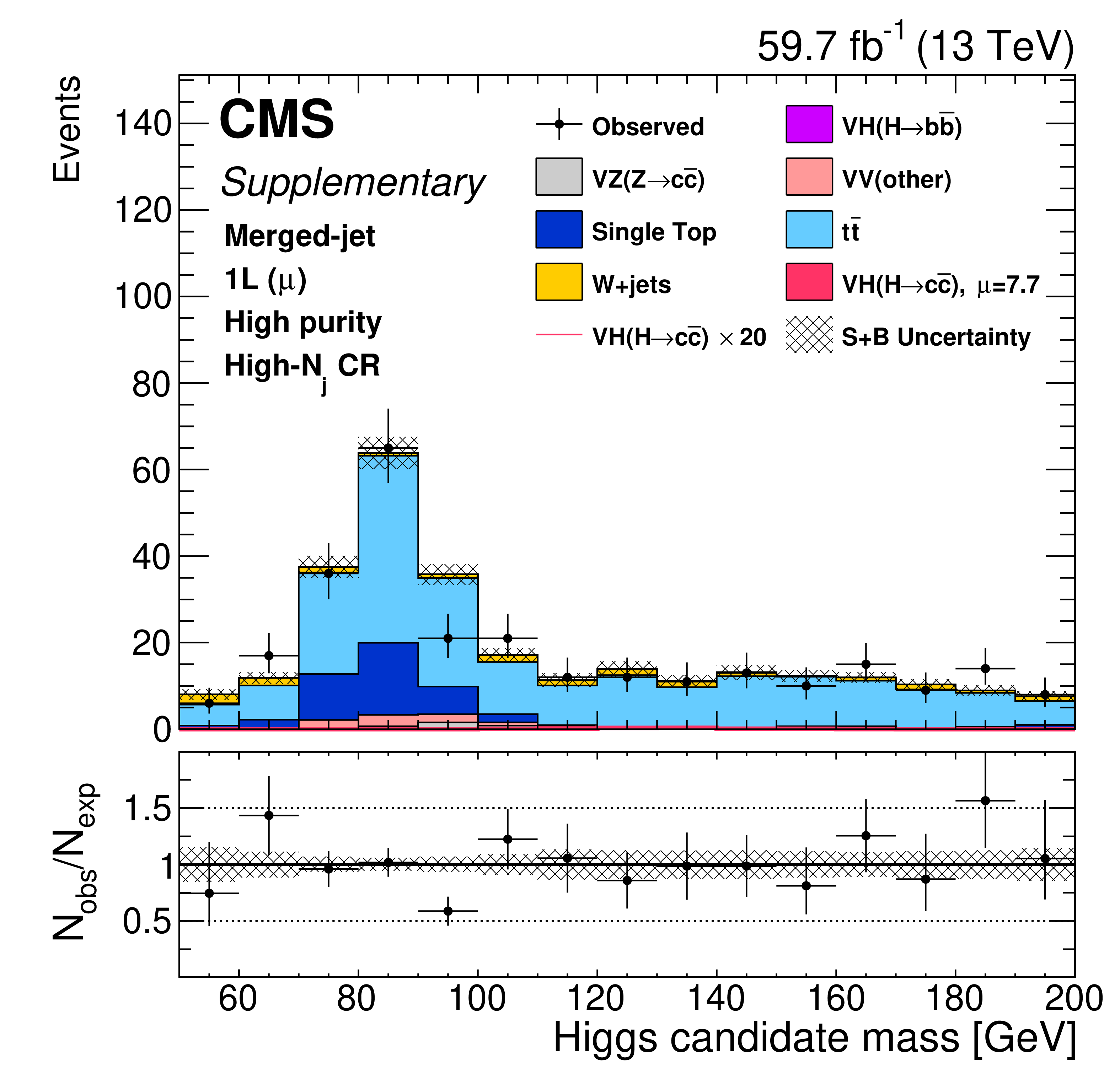
Additional Figure 21:
Post-fit distribution of ${m ({\mathrm{H} _{\text {cand}}} )}$ in the high-$ {N^{\mathrm {aj}}_{\text {small-}R}}$ and high $\mathrm{c} \mathrm{\bar{c}} $-purity control region of the merged-jet topology in the 1L($\mu $) channel in 2018 data. The VH(H $\to \mathrm{c\bar{c}}$) signal yield is scaled by the best fit signal strength, $ {\mu _{{{\mathrm{V} \mathrm{H} (\mathrm{H} \to \mathrm{c} \mathrm{\bar{c}})}}}} =$ 7.7, in the filled red histogram, and the red line represents the expected signal contribution multiplied by a factor of 20. |
png pdf |
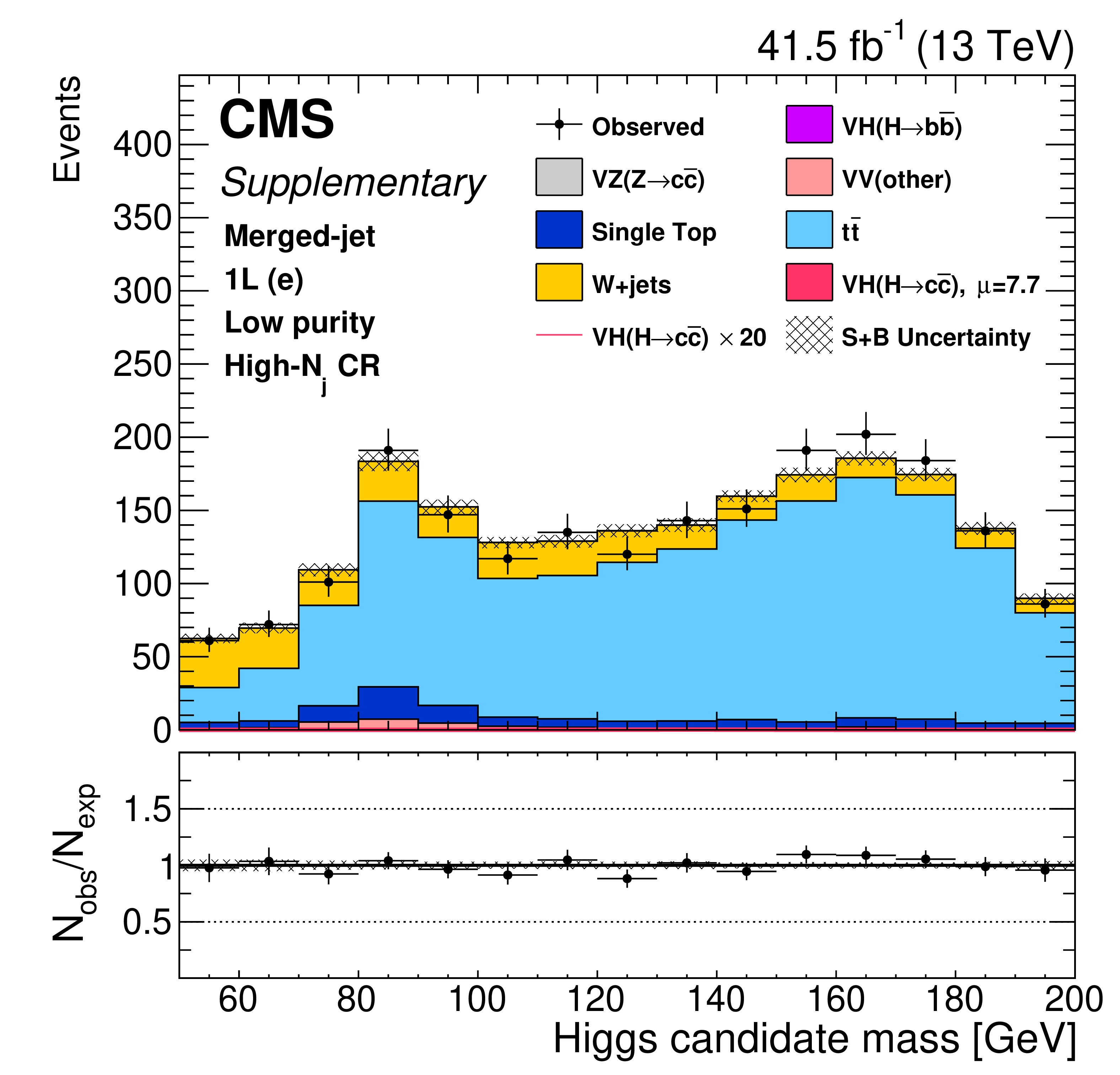
Additional Figure 22:
Post-fit distribution of ${m ({\mathrm{H} _{\text {cand}}} )}$ in the high-$ {N^{\mathrm {aj}}_{\text {small-}R}}$ and low $\mathrm{c} \mathrm{\bar{c}} $-purity control region of the merged-jet topology in the 1L(e) channel in 2017 data. The VH(H $\to \mathrm{c\bar{c}}$) signal yield is scaled by the best fit signal strength, $ {\mu _{{{\mathrm{V} \mathrm{H} (\mathrm{H} \to \mathrm{c} \mathrm{\bar{c}})}}}} =$ 7.7, in the filled red histogram, and the red line represents the expected signal contribution multiplied by a factor of 20. |
png pdf |
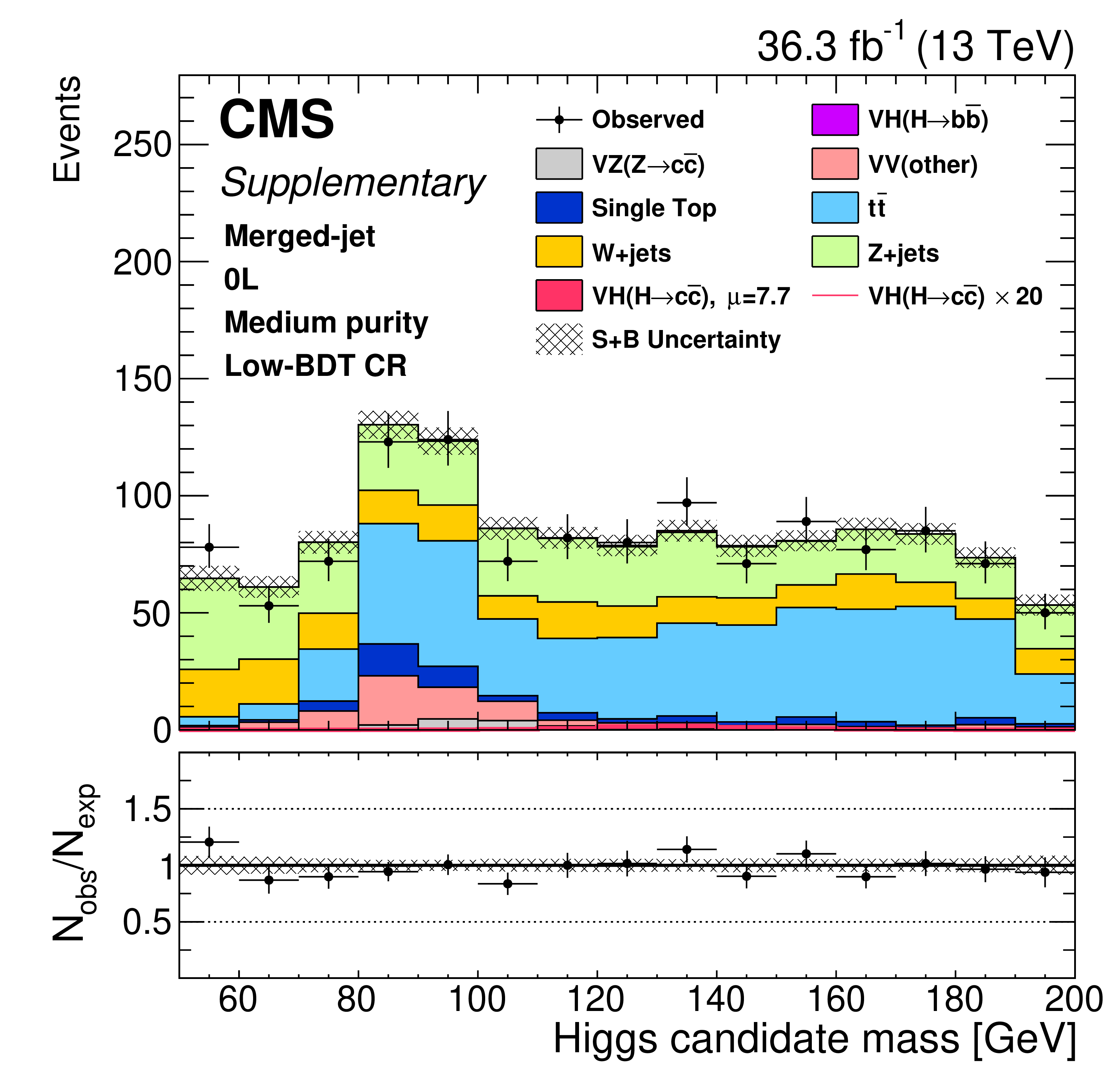
Additional Figure 23:
Post-fit distribution of ${m ({\mathrm{H} _{\text {cand}}} )}$ in the low-BDT and medium $\mathrm{c} \mathrm{\bar{c}} $-purity control region of the merged-jet topology in the 0L channel in 2016 data. The VH(H $\to \mathrm{c\bar{c}}$) signal yield is scaled by the best fit signal strength, $ {\mu _{{{\mathrm{V} \mathrm{H} (\mathrm{H} \to \mathrm{c} \mathrm{\bar{c}})}}}} =$ 7.7, in the filled red histogram, and the red line represents the expected signal contribution multiplied by a factor of 20. |
png pdf |
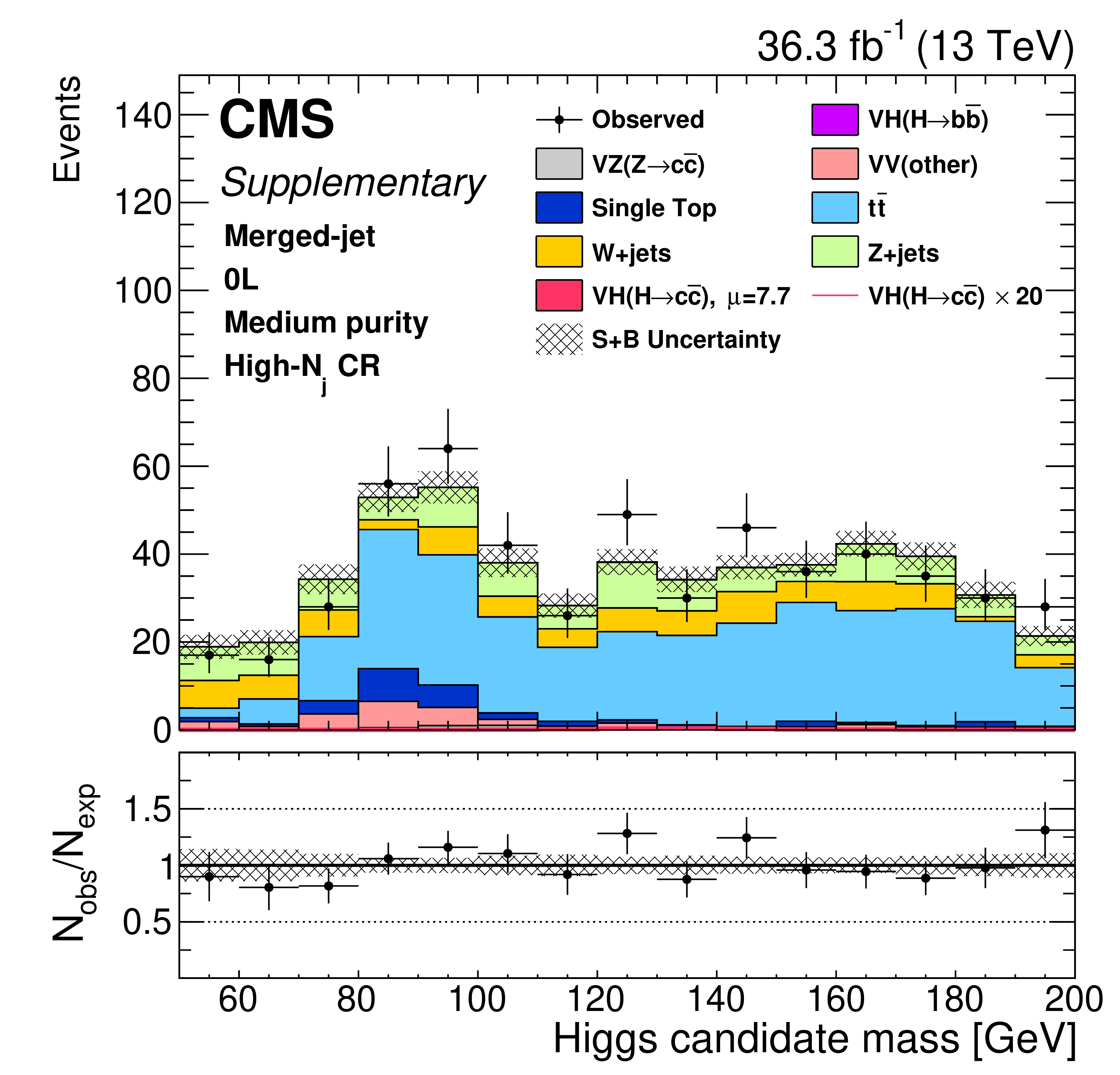
Additional Figure 24:
Post-fit distribution of ${m ({\mathrm{H} _{\text {cand}}} )}$ in the high-$ {N^{\mathrm {aj}}_{\text {small-}R}}$ and medium $\mathrm{c} \mathrm{\bar{c}} $-purity control region of the merged-jet topology in the 0L channel in 2016 data. The VH(H $\to \mathrm{c\bar{c}}$) signal yield is scaled by the best fit signal strength, $ {\mu _{{{\mathrm{V} \mathrm{H} (\mathrm{H} \to \mathrm{c} \mathrm{\bar{c}})}}}} =$ 7.7, in the filled red histogram, and the red line represents the expected signal contribution multiplied by a factor of 20. |
png pdf |
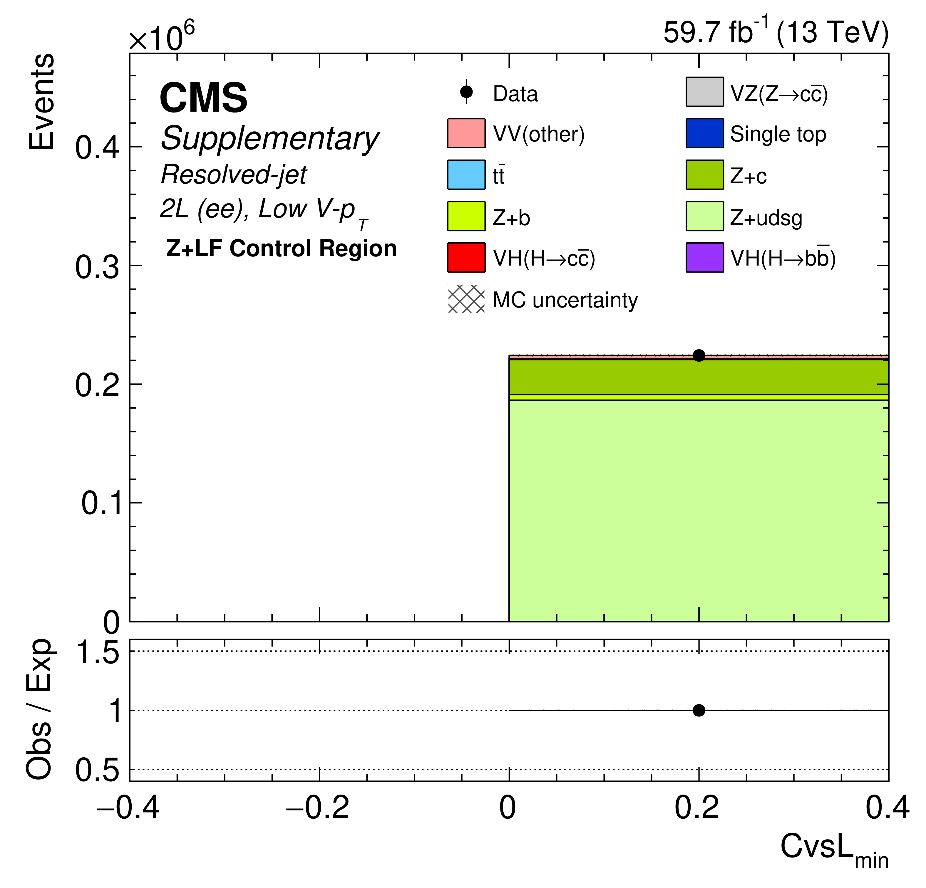
Additional Figure 25:
Post-fit distribution of the $CvsL_{\text {min}}$ discriminant in the low-$ {{p_{\mathrm {T}}} (\mathrm{V})}$ Z+LF control region of the resolved-jet topology in the 2L(ee) channel in 2018 data. |

png pdf |
Additional Figure 26:
Post-fit distribution of the $CvsB_{\text {min}}$ discriminant in the low-$ {{p_{\mathrm {T}}} (\mathrm{V})}$ Z+HF control region of the resolved-jet topology in the 2L(ee) channel in 2018 data. |
png pdf |
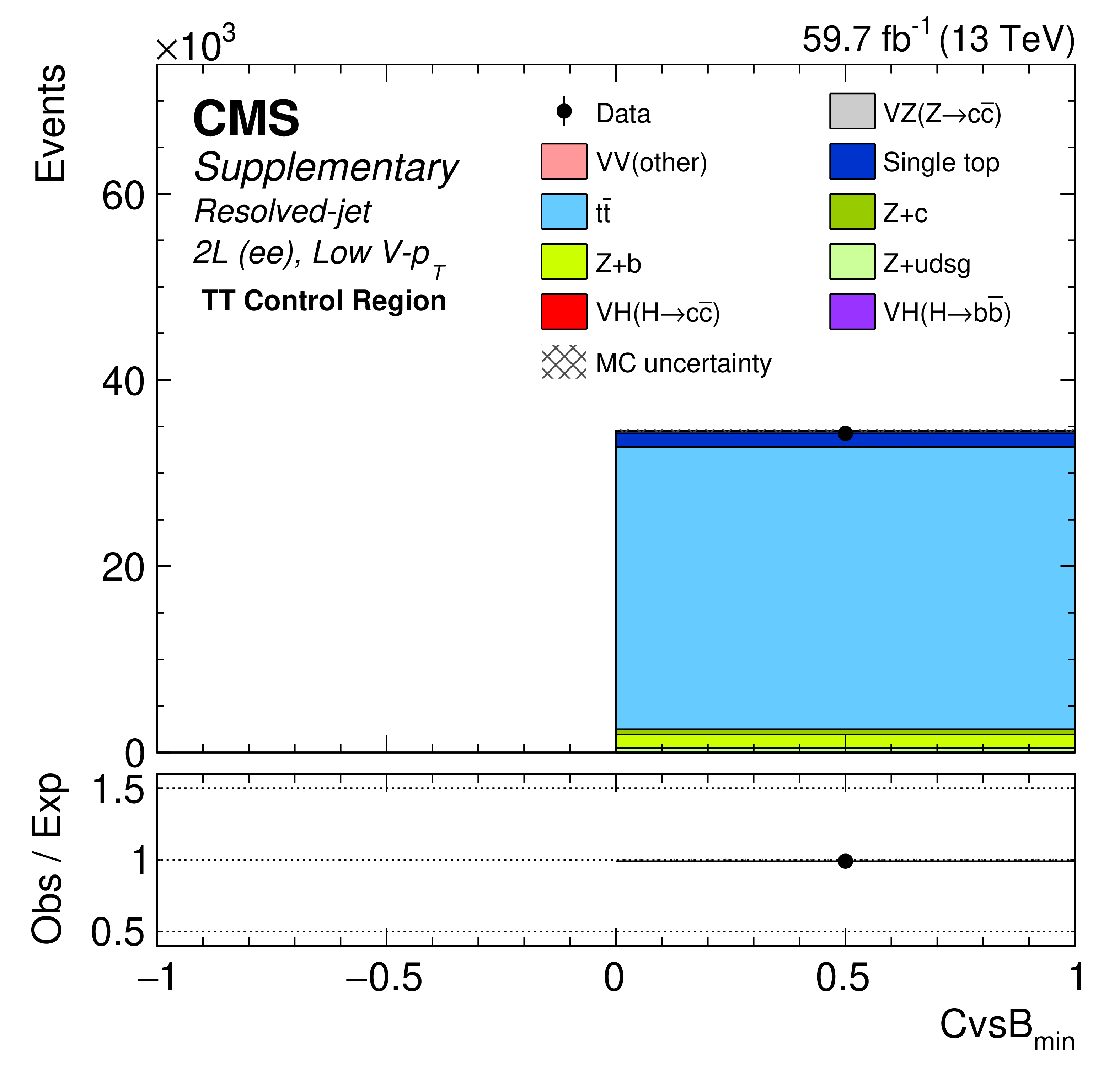
Additional Figure 27:
Post-fit distribution of the $CvsB_{\text {min}}$ discriminant in the low-$ {{p_{\mathrm {T}}} (\mathrm{V})}$ TT control region of the resolved-jet topology in the 2L(ee) channel in 2018 data. |
png pdf |
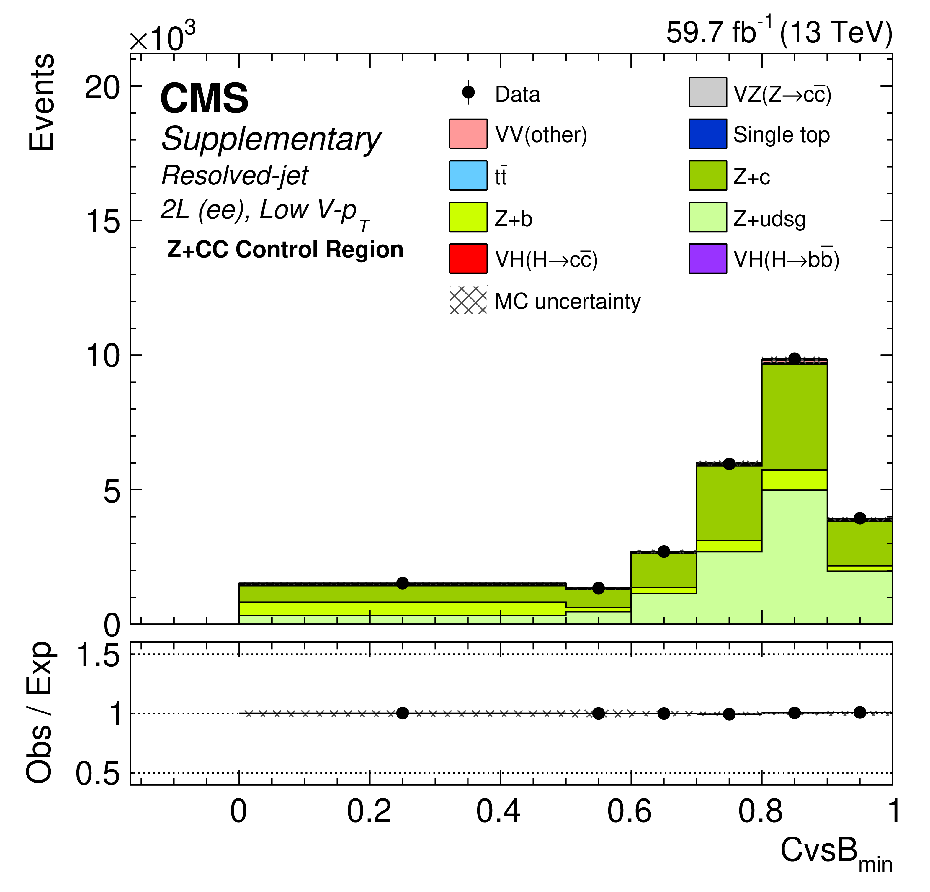
Additional Figure 28:
Post-fit distribution of the $CvsB_{\text {min}}$ discriminant in the low-$ {{p_{\mathrm {T}}} (\mathrm{V})}$ Z+CC control region of the resolved-jet topology in the 2L(ee) channel in 2018 data. |

png pdf |
Additional Figure 29:
Post-fit distribution of the $CvsB_{\text {min}}$ discriminant in the W+CC control region of the resolved-jet topology in the 1L($\mu $) channel in 2018 data. |
png pdf |
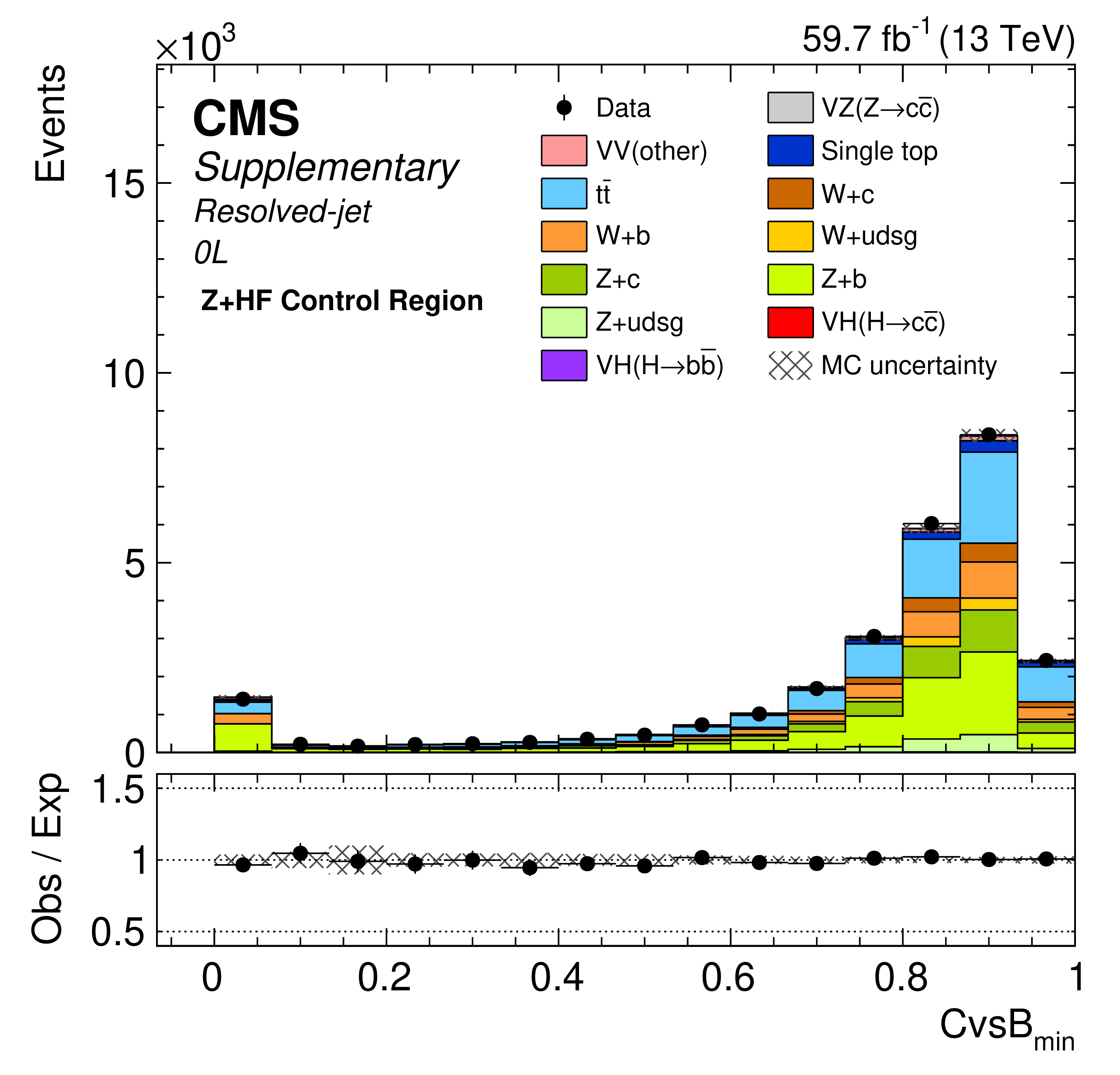
Additional Figure 30:
Post-fit distribution of the $CvsB_{\text {min}}$ discriminant in the Z+HF control region of the resolved-jet topology in the 0L channel in 2018 data. |
png pdf |
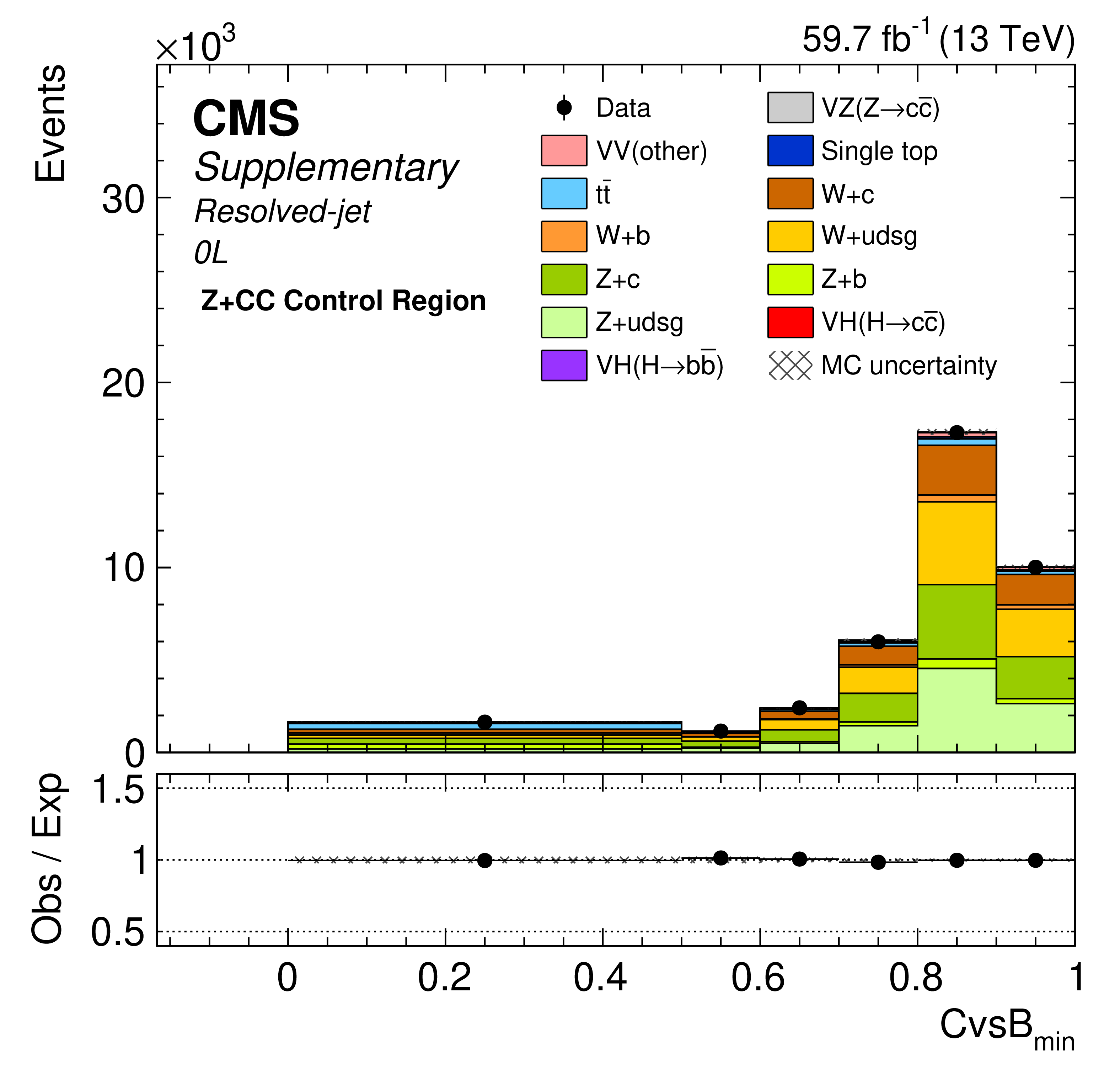
Additional Figure 31:
Post-fit distribution of the $CvsB_{\text {min}}$ discriminant in the Z+CC control region of the resolved-jet topology in the 0L channel in 2018 data. |
png pdf |
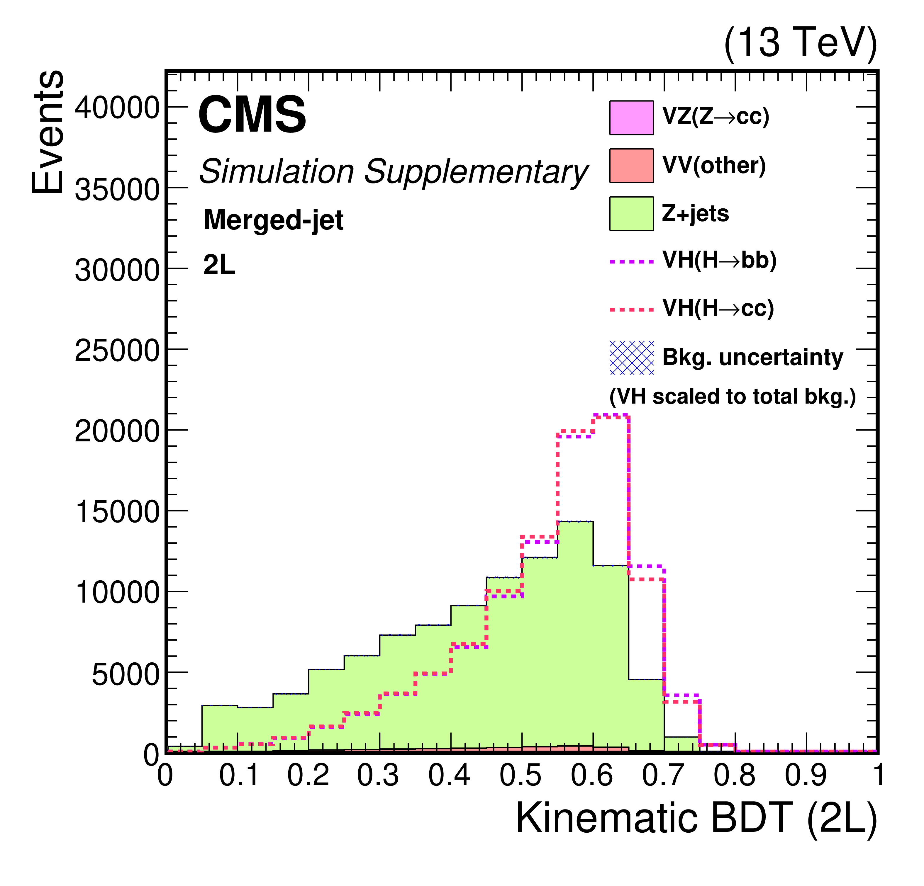
Additional Figure 32:
Distribution of the kinematic BDT in the 2L channel of the merged-jet analysis. The VH(H $\to \mathrm{c\bar{c}}$) signal is normalized to the sum of all backgrounds. The VH(H $\to \mathrm{b\bar{b}}$) contribution, similarly normalized, is also shown. |
png pdf |
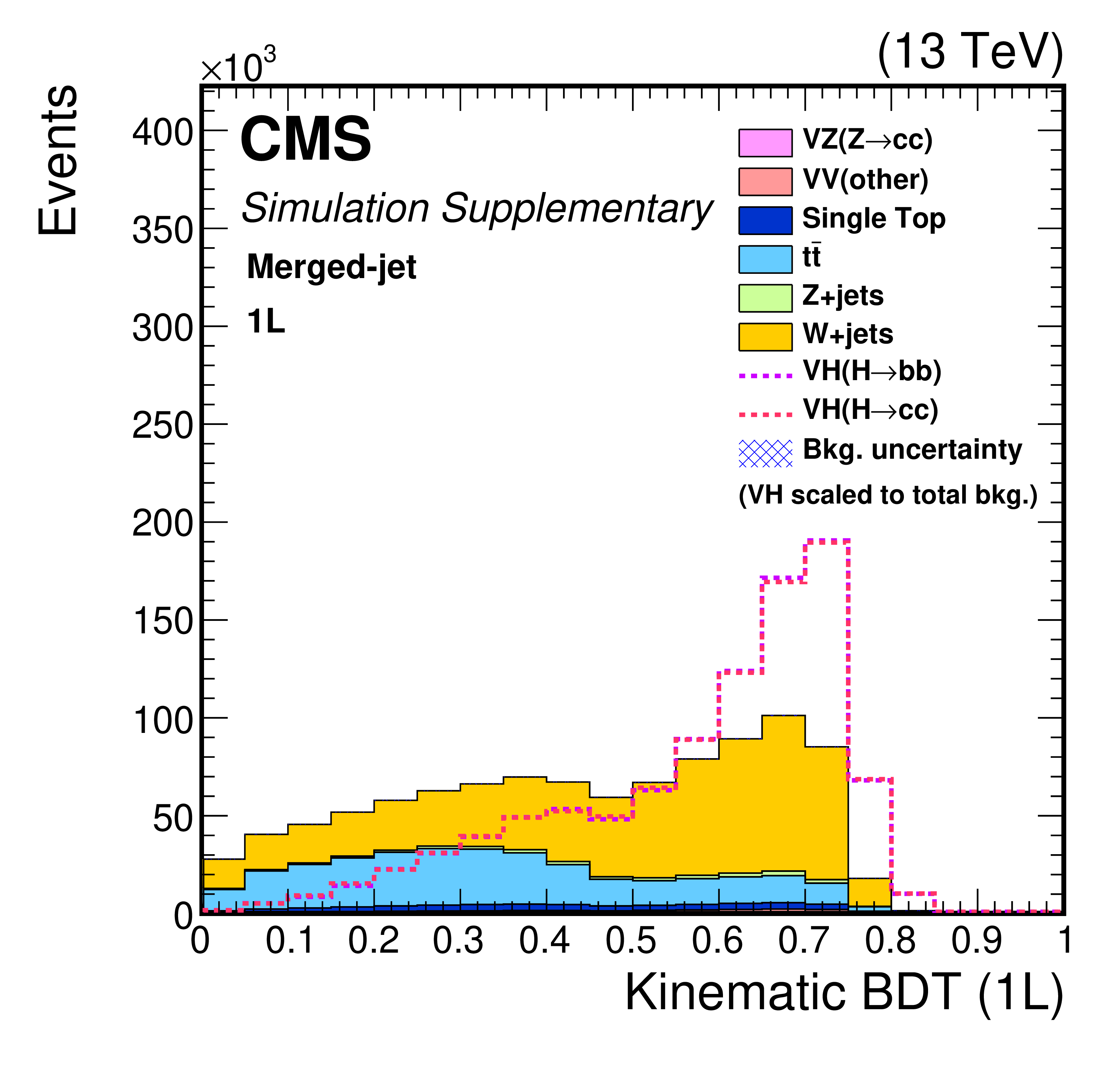
Additional Figure 33:
Distribution of the kinematic BDT in the 1L channel of the merged-jet analysis. The VH(H $\to \mathrm{c\bar{c}}$) signal is normalized to the sum of all backgrounds. The VH(H $\to \mathrm{b\bar{b}}$) contribution, similarly normalized, is also shown. |
png pdf |
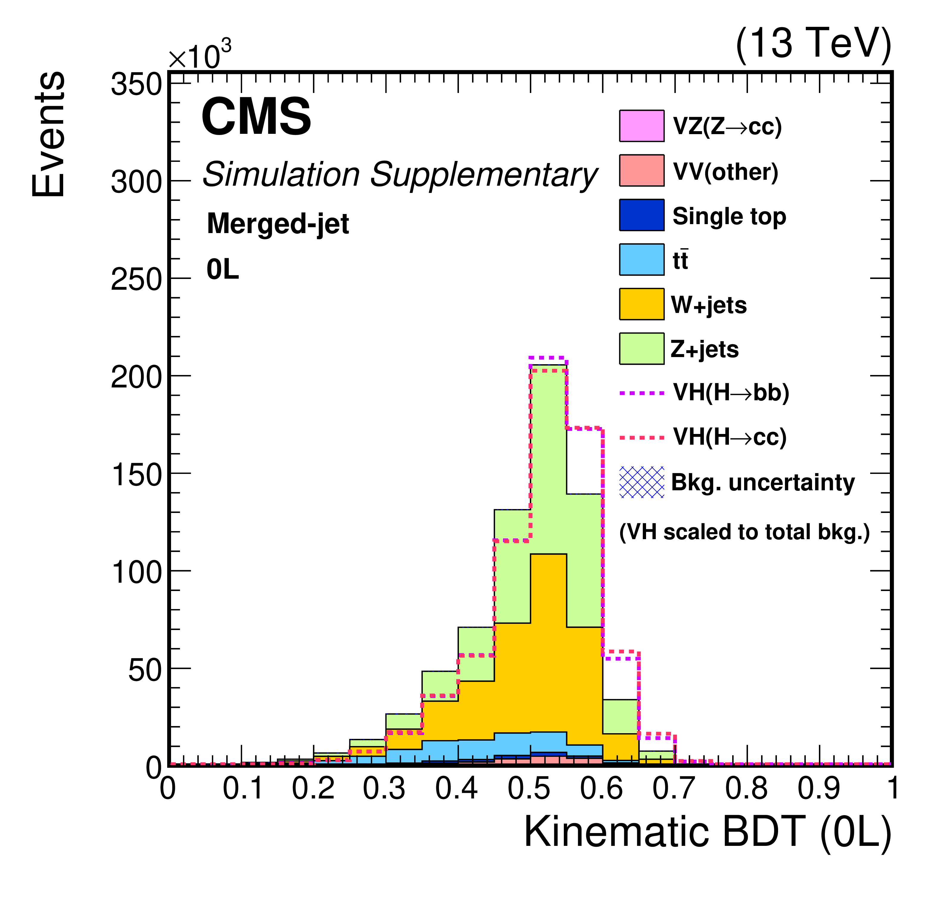
Additional Figure 34:
Distribution of the kinematic BDT in the 0L channel of the merged-jet analysis. The VH(H $\to \mathrm{c\bar{c}}$) signal is normalized to the sum of all backgrounds. The VH(H $\to \mathrm{b\bar{b}}$) contribution, similarly normalized, is also shown. |

png pdf |
Additional Figure 35:
Distribution of the ParticleNet cc-tagging discriminant for events with BDT scores greater than 0.55 in the 2L channel of the merged-jet analysis. The VH(H $\to \mathrm{c\bar{c}}$) signal is normalized to the sum of all backgrounds. The VH(H $\to \mathrm{b\bar{b}}$) contribution, similarly normalized, is also shown. |

png pdf |
Additional Figure 36:
Distribution of the ParticleNet cc-tagging discriminant for events with BDT scores greater than 0.7 in the 1L channel of the merged-jet analysis. The VH(H $\to \mathrm{c\bar{c}}$) signal is normalized to the sum of all backgrounds. The VH(H $\to \mathrm{b\bar{b}}$) contribution, similarly normalized, is also shown. |

png pdf |
Additional Figure 37:
Distribution of the ParticleNet cc-tagging discriminant for events with BDT scores greater than 0.55 in the 0L channel of the merged-jet analysis. The VH(H $\to \mathrm{c\bar{c}}$) signal is normalized to the sum of all backgrounds. The VH(H $\to \mathrm{b\bar{b}}$) contribution, similarly normalized, is also shown. |
png pdf |
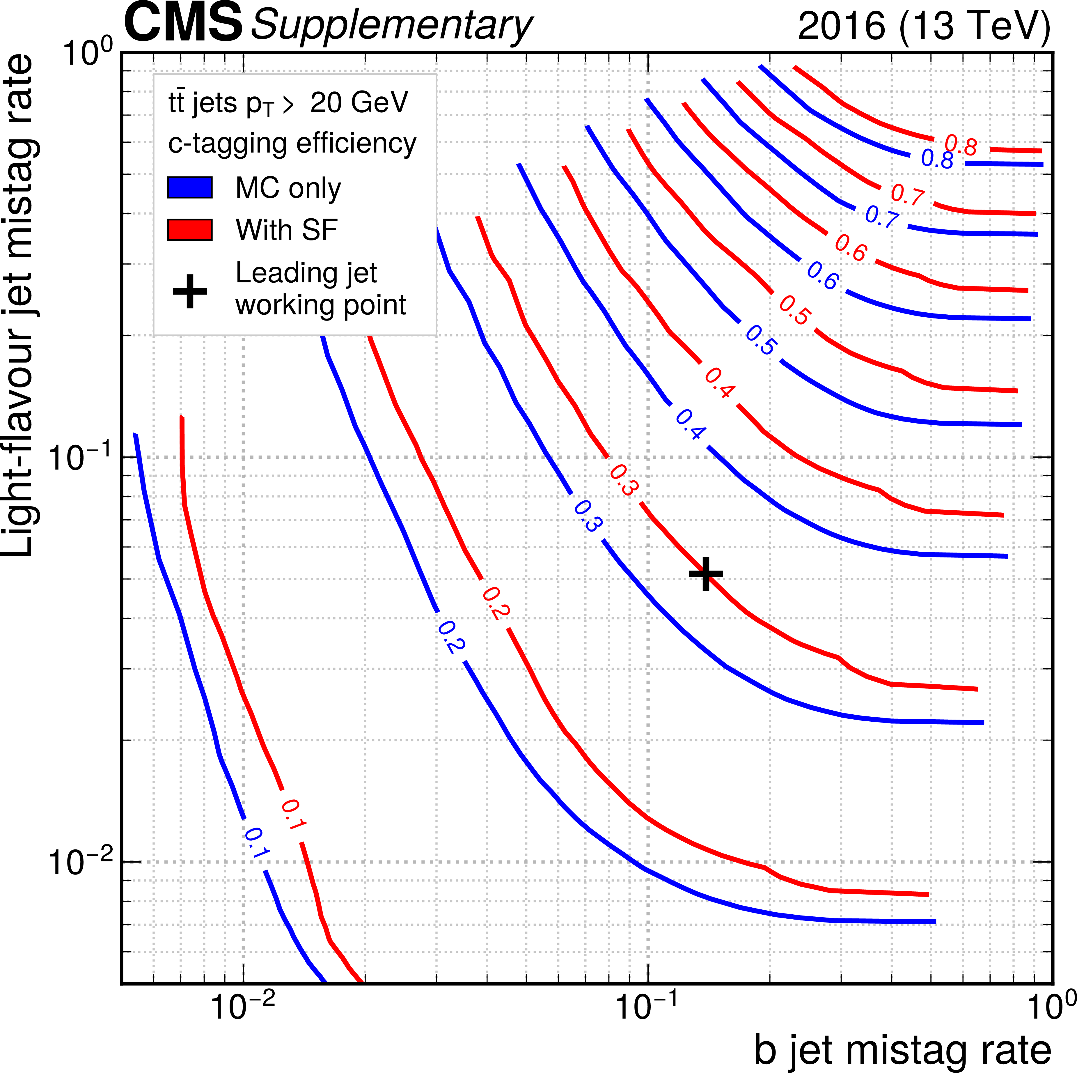
Additional Figure 38:
Performance of the DeepJet-based c-tagging algorithm for small-$R$ jets, with (red) and without (blue) the application of the data-to-simulation scale factors (SFs). Each curve is an iso-efficiency curve representing a specific c-jet efficiency. The horizontal (vertical) axis represents the mis-identification rate of b jets (light quark or gluon jets). The result is obtained with a 2016 ${\mathrm{t} \mathrm{\bar{t}}}$ simulated sample, requiring a threshold of 20 GeV on the jet transverse momentum. The black cross represents the working point applied to the leading jet in the analysis, requiring $CvsL > 0.225$ and $CvsB > 0.4$. |
png pdf |
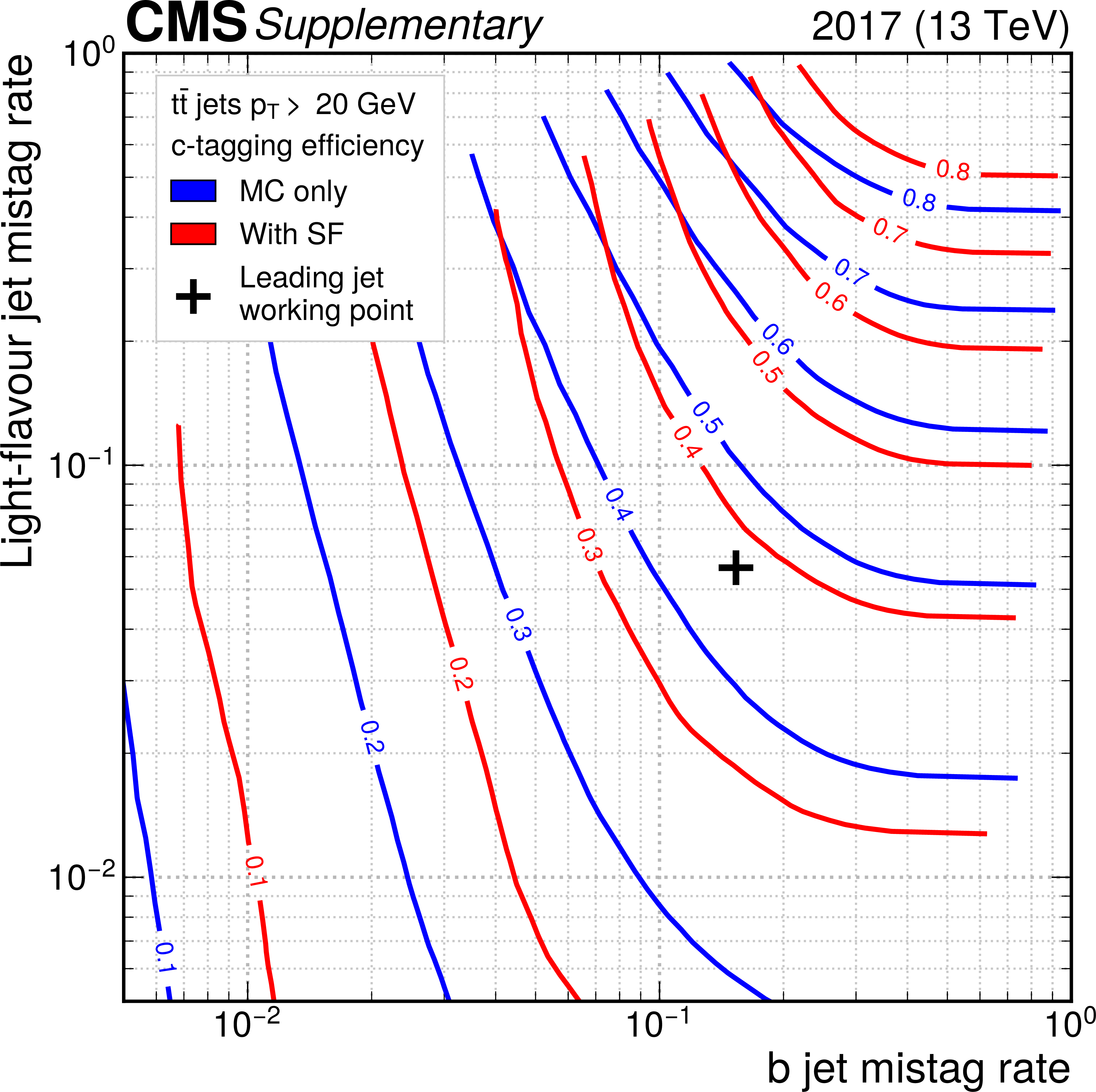
Additional Figure 39:
Performance of the DeepJet-based c-tagging algorithm for small-$R$ jets, with (red) and without (blue) the application of the data-to-simulation scale factors (SFs). Each curve is an iso-efficiency curve representing a specific c-jet efficiency. The horizontal (vertical) axis represents the mis-identification rate of b jets (light quark or gluon jets). The result is obtained with a 2017 ${\mathrm{t} \mathrm{\bar{t}}}$ simulated sample, requiring a threshold of 20 GeV on the jet transverse momentum. The black cross represents the working point applied to the leading jet in the analysis, requiring $CvsL > 0.225$ and $CvsB > 0.4$. |
png pdf |
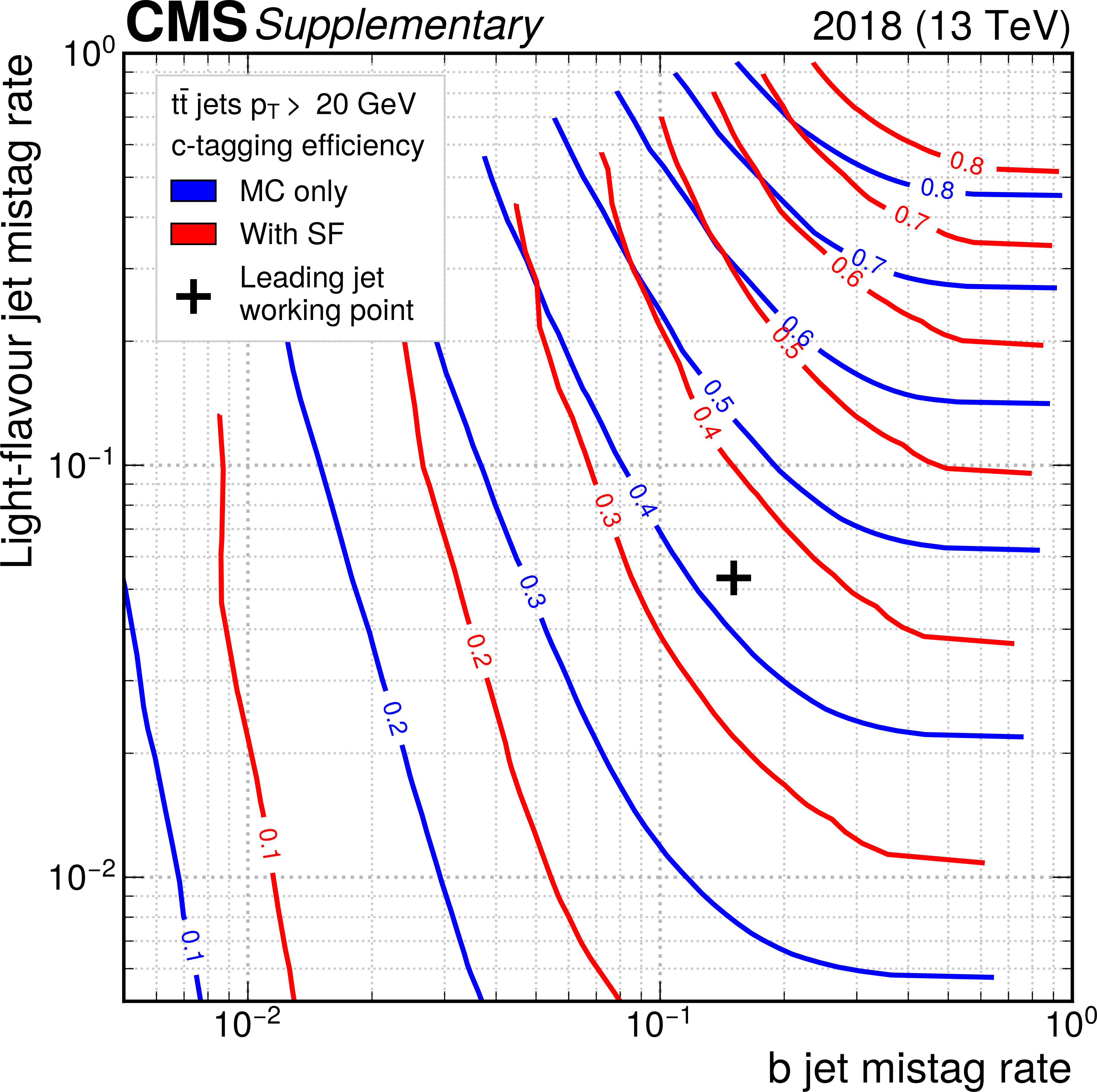
Additional Figure 40:
Performance of the DeepJet-based c-tagging algorithm for small-$R$ jets, with (red) and without (blue) the application of the data-to-simulation scale factors (SFs). Each curve is an iso-efficiency curve representing a specific c-jet efficiency. The horizontal (vertical) axis represents the mis-identification rate of b jets (light quark or gluon jets). The result is obtained with a 2018 ${\mathrm{t} \mathrm{\bar{t}}}$ simulated sample, requiring a threshold of 20 GeV on the jet transverse momentum. The black cross represents the working point applied to the leading jet in the analysis, requiring $CvsL > 0.225$ and $CvsB > 0.4$. |
png pdf |
Additional Figure 41:
Distribution of ${m ({\mathrm{H} _{\text {cand}}} )}$ for simulated VH(H $\to \mathrm{c\bar{c}}$) signal events with 60 $< {{p_{\mathrm {T}}} (\mathrm{V})} < $ 150 GeV in the 2L channel in 2016. The red histogram corresponds to the distribution without applying the c-jet energy regression nor the kinematic fit, the green histogram corresponds to the distribution after the application of the c-jet energy regression, and the blue histogram represents the distribution after the application of both the c-jet energy regression and the kinematic fit. The dashed lines represent the fitted shapes using double crystal-ball functions. |
png pdf |
Additional Figure 42:
Distribution of ${m ({\mathrm{H} _{\text {cand}}} )}$ for simulated VH(H $\to \mathrm{c\bar{c}}$) signal events with ${{{p_{\mathrm {T}}} (\mathrm{V})} } > $ 150 GeV in the 2L channel in 2016. The red histogram corresponds to the distribution without applying the c-jet energy regression nor the kinematic fit, the green histogram corresponds to the distribution after the application of the c-jet energy regression, and the blue histogram represents the distribution after the application of both the c-jet energy regression and the kinematic fit. The dashed lines represent the fitted shapes using double crystal-ball functions. |
png pdf |
Additional Figure 43:
Distribution of ${m ({\mathrm{H} _{\text {cand}}} )}$ for simulated VH(H $\to \mathrm{c\bar{c}}$) signal events with 60 $< {{p_{\mathrm {T}}} (\mathrm{V})} < $ 150 GeV in the 2L channel in 2017. The red histogram corresponds to the distribution without applying the c-jet energy regression nor the kinematic fit, the green histogram corresponds to the distribution after the application of the c-jet energy regression, and the blue histogram represents the distribution after the application of both the c-jet energy regression and the kinematic fit. The dashed lines represent the fitted shapes using double crystal-ball functions. |

png pdf |
Additional Figure 44:
Distribution of ${m ({\mathrm{H} _{\text {cand}}} )}$ for simulated VH(H $\to \mathrm{c\bar{c}}$) signal events with ${{{p_{\mathrm {T}}} (\mathrm{V})} } > $ 150 GeV in the 2L channel in 2017. The red histogram corresponds to the distribution without applying the c-jet energy regression nor the kinematic fit, the green histogram corresponds to the distribution after the application of the c-jet energy regression, and the blue histogram represents the distribution after the application of both the c-jet energy regression and the kinematic fit. The dashed lines represent the fitted shapes using double crystal-ball functions. |

png pdf |
Additional Figure 45:
Distribution of ${m ({\mathrm{H} _{\text {cand}}} )}$ for simulated VH(H $\to \mathrm{c\bar{c}}$) signal events with 60 $< {{p_{\mathrm {T}}} (\mathrm{V})} < $ 150 GeV in the 2L channel in 2018. The red histogram corresponds to the distribution without applying the c-jet energy regression nor the kinematic fit, the green histogram corresponds to the distribution after the application of the c-jet energy regression, and the blue histogram represents the distribution after the application of both the c-jet energy regression and the kinematic fit. The dashed lines represent the fitted shapes using double crystal-ball functions. |
png pdf |
Additional Figure 46:
Distribution of ${m ({\mathrm{H} _{\text {cand}}} )}$ for simulated VH(H $\to \mathrm{c\bar{c}}$) signal events with ${{{p_{\mathrm {T}}} (\mathrm{V})} } > $ 150 GeV in the 2L channel in 2018. The red histogram corresponds to the distribution without applying the c-jet energy regression nor the kinematic fit, the green histogram corresponds to the distribution after the application of the c-jet energy regression, and the blue histogram represents the distribution after the application of both the c-jet energy regression and the kinematic fit. The dashed lines represent the fitted shapes using double crystal-ball functions. |
png pdf |
Additional Figure 47:
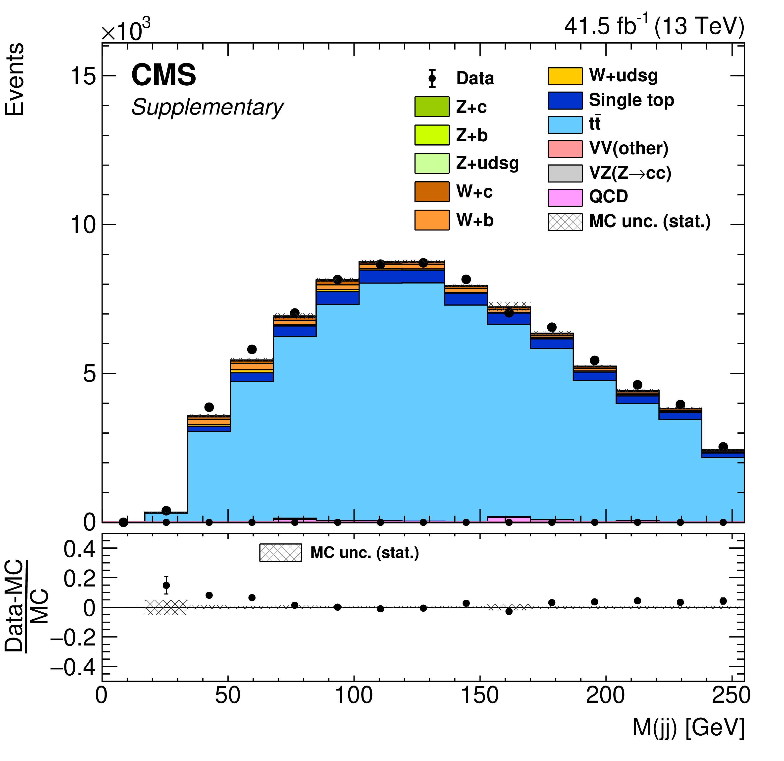
Distribution of the reconstructed di-jet invariant mass in the TT control region of the 1L(e) channel in 2017 data after the application of the c-jet energy regression. |
png pdf |
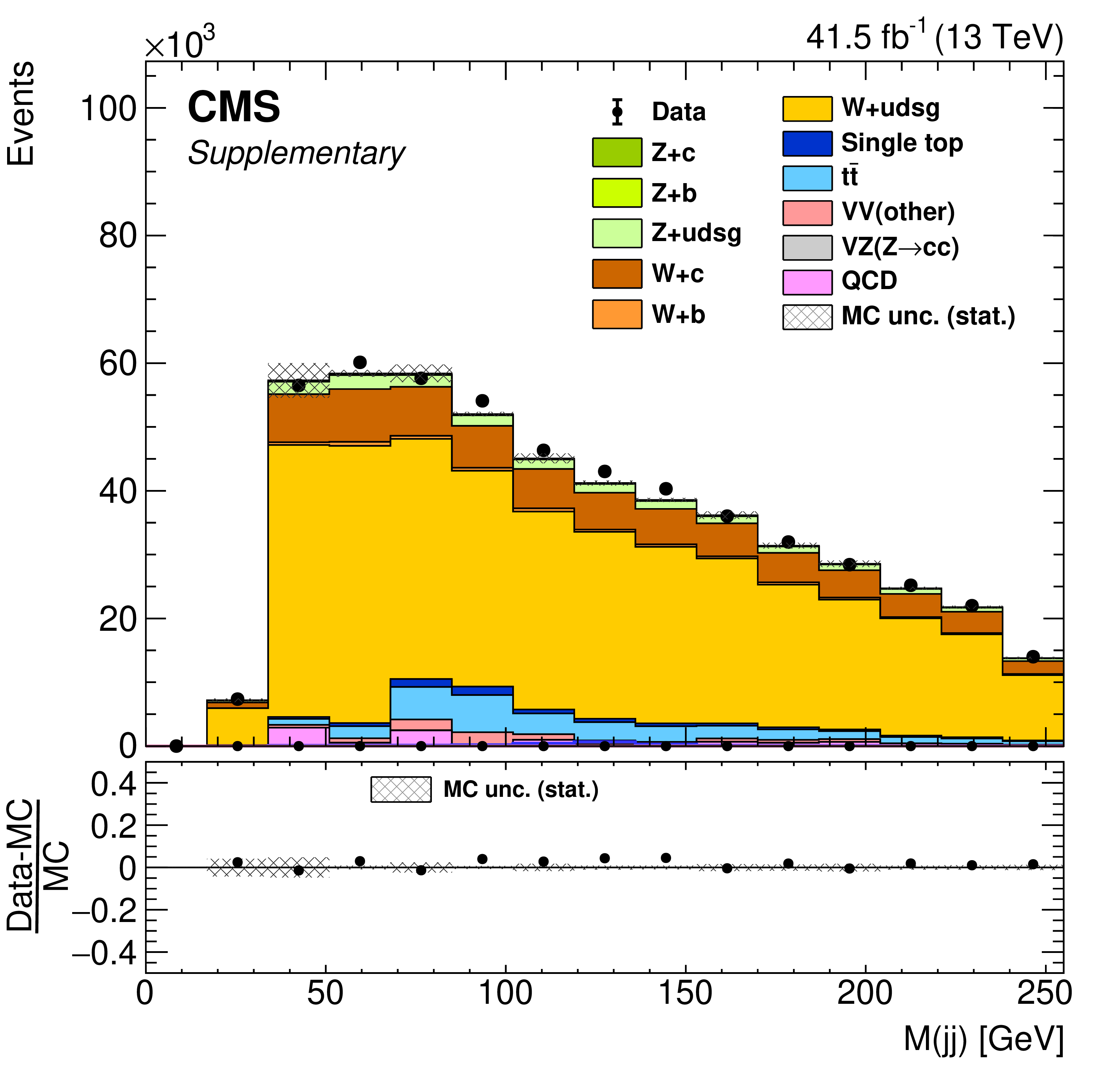
Additional Figure 48:
Distribution of the reconstructed di-jet invariant mass in the W+LF control region of the 1L(e) channel in 2017 data after the application of the c-jet energy regression. |

png pdf |
Additional Figure 49:
Extrapolation of the sensitivity to H $\to \mathrm{ b\bar{b} }$ and H $\to \mathrm{ c\bar{c} }$ decays at the HL-LHC, shown as the profile likelihood scan as a function of the signal strengths $\mu _{{{\mathrm{V} \mathrm{H} (\mathrm{H} \to \mathrm{c} \mathrm{\bar{c}})}}}$ and $\mu _{{{\mathrm{V} \mathrm{H} (\mathrm{H} \to \mathrm{b} \mathrm{\bar{b}})}}}$. The solid symbol shows the SM expected point. The solid and dashed lines show the expected one and two standard deviation contours. The projection is based on the merged-jet topology with the following modifications: the large-$R$ jet ${p_{\mathrm {T}}}$ threshold is lowered to 200 GeV, and 3 categories enriched in H $\to \mathrm{ b\bar{b} }$ decays, defined with the ParticleNet $\mathrm{b} \mathrm{\bar{b}} $ discriminant, are added to allow for a simultaneous measurement of the VH(H $\to \mathrm{b\bar{b}}$) and VH(H $\to \mathrm{c\bar{c}}$) processes. Signal and background yields are scaled to an integrated luminosity of 3000 fb$^{-1}$ and higher production cross sections at $\sqrt {s} = $ 14 TeV. The systematic uncertainties are adjusted according to the YR18 prescription [101]. Specifically, the theoretical uncertainties are reduced to half of the Run 2 values, and most of the experimental uncertainties are scaled down with the square root of the integrated luminosity. The uncertainties on the $\mathrm{b} \mathrm{\bar{b}} $ and $\mathrm{c} \mathrm{\bar{c}} $ tagging efficiencies are constrained by the VZ(Z $\to \mathrm{b\bar{b}}$) and VZ(Z $\to \mathrm{c\bar{c}}$) events to approximately 3% and 5%, respectively. The uncertainty on the misidentification of H $\to \mathrm{b\bar{b}}$ as H $\to \mathrm{c\bar{c}}$ is assumed to be 20%. |

png pdf |
Additional Figure 50:
Extrapolation of the sensitivity to H $\to \mathrm{ b\bar{b} }$ and H $\to \mathrm{ c\bar{c} }$ decays at the HL-LHC, shown as the profile likelihood scan as a function of the coupling modifiers ${\kappa _{\mathrm{b}}}$ and ${\kappa _{\mathrm{c}}}$. The solid symbol shows the SM expected point. The solid and dashed lines show the expected one and two standard deviation contours. The projection is based on the merged-jet topology with the following modifications: the large-$R$ jet ${p_{\mathrm {T}}}$ threshold is lowered to 200 GeV, and 3 categories enriched in H $\to \mathrm{ b\bar{b} }$ decays, defined with the ParticleNet $\mathrm{b} \mathrm{\bar{b}} $ discriminant, are added to allow for a simultaneous measurement of the VH(H $\to \mathrm{b\bar{b}}$) and VH(H $\to \mathrm{c\bar{c}}$) processes. Signal and background yields are scaled to an integrated luminosity of 3000 fb$^{-1}$ and higher production cross sections at $\sqrt {s} = $ 14 TeV. The systematic uncertainties are adjusted according to the YR18 prescription [101]. Specifically, the theoretical uncertainties are reduced to half of the Run 2 values, and most of the experimental uncertainties are scaled down with the square root of the integrated luminosity. The uncertainties on the $\mathrm{b} \mathrm{\bar{b}} $ and $\mathrm{c} \mathrm{\bar{c}} $ tagging efficiencies are constrained by the VZ(Z $\to \mathrm{b\bar{b}}$) and VZ(Z $\to \mathrm{c\bar{c}}$) events to approximately 3% and 5%, respectively. The uncertainty on the misidentification of H $\to \mathrm{b\bar{b}}$ as H $\to \mathrm{c\bar{c}}$ is assumed to be 20%. |
| Additional Tables | |
png pdf |
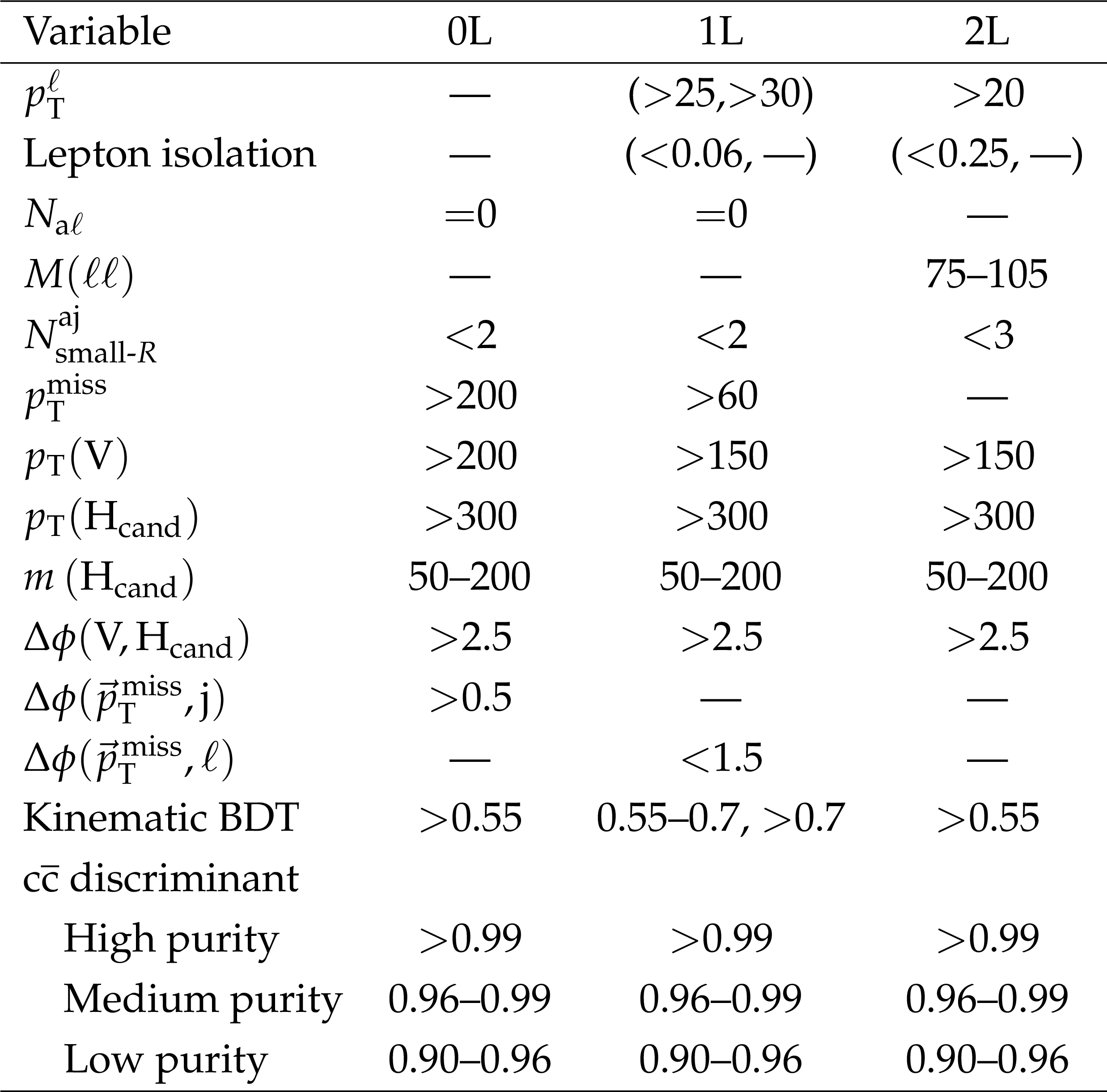
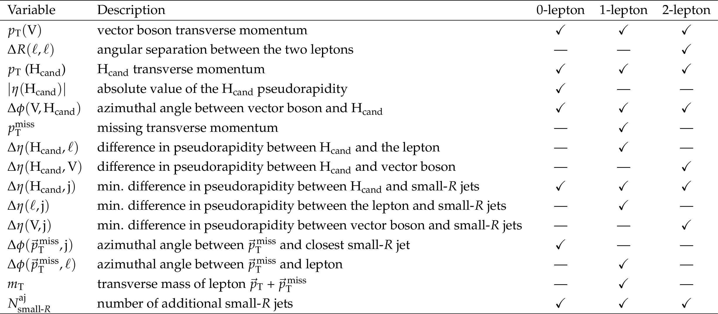
Additional Table 1:
Event selection criteria for the signal region in the merged-jet analysis. Entries marked with "--'' indicate that the variable is not used in the given channel. The values listed for kinematic variables are in units of GeV, and for angles in units of radians. Where selection differs between lepton flavors, the selection is listed as (muon, electron). |
png pdf |
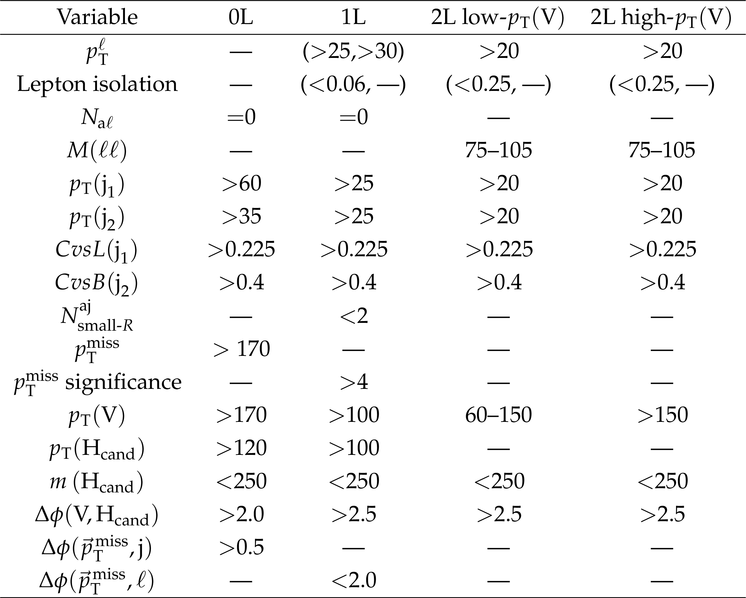
Additional Table 2:
Event selection criteria for the signal region in the resolved-jet analysis. Entries marked with "--'' indicate that the variable is not used in the given channel. The values listed for kinematic variables are in units of GeV, and for angles in units of radians. Where selection differs between lepton flavors, the selection is listed as (muon, electron). |
png pdf |
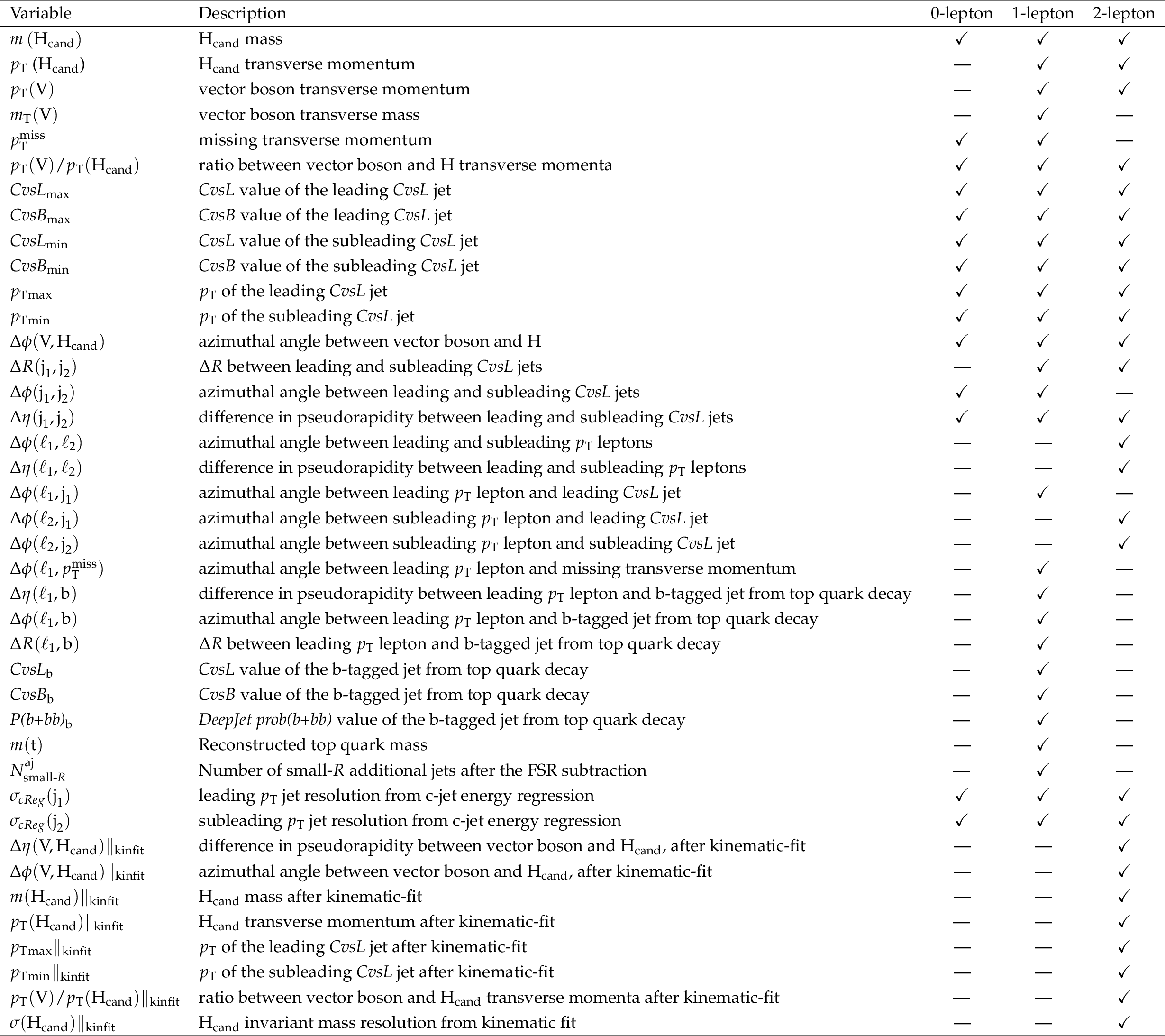
Additional Table 3:
Variables used in the kinematic BDT training for each channel of the merged-jet analysis. |
png pdf |
Additional Table 4:
Variables employed in the training of the BDT used for each channel of the resolved-jet analysis. |
png pdf |
Additional Table 5:
The relative contributions to the total uncertainty on ${\mu _{{{\mathrm{V} \mathrm{H} (\mathrm{H} \to \mathrm{c} \mathrm{\bar{c}})}}}}$ in the merged-jet analysis, with a best fit value $ {\mu _{{{\mathrm{V} \mathrm{H} (\mathrm{H} \to \mathrm{c} \mathrm{\bar{c}})}}}} = $ 8.7$^{+4.6}_{-4.0}$. |

png pdf |
Additional Table 6:
The relative contributions to the total uncertainty on ${\mu _{{{\mathrm{V} \mathrm{H} (\mathrm{H} \to \mathrm{c} \mathrm{\bar{c}})}}}}$ in the resolved-jet analysis, with a best fit value $ {\mu _{{{\mathrm{V} \mathrm{H} (\mathrm{H} \to \mathrm{c} \mathrm{\bar{c}})}}}} = -$9.5 $\pm$ 9.6. |
| References | ||||
| 1 | ATLAS Collaboration | Observation of a new particle in the search for the standard model Higgs boson with the ATLAS detector at the LHC | PLB 716 (2012) 1 | 1207.7214 |
| 2 | CMS Collaboration | Observation of a new boson at a mass of 125 GeV with the CMS experiment at the LHC | PLB 716 (2012) 30 | CMS-HIG-12-028 1207.7235 |
| 3 | CMS Collaboration | Observation of a new boson with mass near 125 GeV in pp collisions at $ \sqrt{s} = $ 7 and 8 TeV | JHEP 06 (2013) 081 | CMS-HIG-12-036 1303.4571 |
| 4 | CMS Collaboration | A measurement of the Higgs boson mass in the diphoton decay channel | PLB 805 (2020) 135425 | CMS-HIG-19-004 2002.06398 |
| 5 | ATLAS Collaboration | Measurement of Higgs boson production in the diphoton decay channel in pp collisions at center-of-mass energies of 7 and 8 TeV with the ATLAS detector | PRD 90 (2014) 112015 | 1408.7084 |
| 6 | CMS Collaboration | Observation of the diphoton decay of the Higgs boson and measurement of its properties | EPJC 74 (2014) 3076 | CMS-HIG-13-001 1407.0558 |
| 7 | ATLAS Collaboration | Measurements of Higgs boson production and couplings in the four-lepton channel in pp collisions at center-of-mass energies of 7 and 8 TeV with the ATLAS detector | PRD 91 (2015) 012006 | 1408.5191 |
| 8 | CMS Collaboration | Measurement of the properties of a Higgs boson in the four-lepton final state | PRD 89 (2014) 092007 | CMS-HIG-13-002 1312.5353 |
| 9 | ATLAS Collaboration | Observation and measurement of Higgs boson decays to WW$ ^* $ with the ATLAS detector | PRD 92 (2015) 012006 | 1412.2641 |
| 10 | ATLAS Collaboration | Study of (W/Z)H production and Higgs boson couplings using H $ \rightarrow $ WW$ ^{\ast} $ decays with the ATLAS detector | JHEP 08 (2015) 137 | 1506.06641 |
| 11 | CMS Collaboration | Measurement of Higgs boson production and properties in the WW decay channel with leptonic final states | JHEP 01 (2014) 096 | CMS-HIG-13-023 1312.1129 |
| 12 | ATLAS Collaboration | Evidence for the Higgs-boson Yukawa coupling to tau leptons with the ATLAS detector | JHEP 04 (2015) 117 | 1501.04943 |
| 13 | CMS Collaboration | Evidence for the 125 GeV Higgs boson decaying to a pair of $ \tau $ leptons | JHEP 05 (2014) 104 | CMS-HIG-13-004 1401.5041 |
| 14 | CMS Collaboration | Observation of the Higgs boson decay to a pair of tau leptons | PLB 779 (2017) 283 | CMS-HIG-16-043 1708.00373 |
| 15 | CMS Collaboration | Measurements of properties of the Higgs boson decaying to a W boson pair in pp collisions at $ \sqrt{s}= $ 13 TeV | PLB 791 (2019) 96 | CMS-HIG-16-042 1806.05246 |
| 16 | ATLAS Collaboration | Measurements of the Higgs boson production and decay rates and coupling strengths using pp collision data at $ \sqrt{s}= $ 7 and 8 TeV in the ATLAS experiment | EPJC 76 (2016) 6 | 1507.04548 |
| 17 | CMS Collaboration | Precise determination of the mass of the Higgs boson and tests of compatibility of its couplings with the standard model predictions using proton collisions at 7 and 8 TeV | EPJC 75 (2015) 212 | CMS-HIG-14-009 1412.8662 |
| 18 | CMS Collaboration | Study of the mass and spin-parity of the Higgs boson candidate via its decays to Z boson pairs | PRL 110 (2013) 081803 | CMS-HIG-12-041 1212.6639 |
| 19 | ATLAS Collaboration | Evidence for the spin-0 nature of the Higgs boson using ATLAS data | PLB 726 (2013) 120 | 1307.1432 |
| 20 | ATLAS and CMS Collaborations | Measurements of the Higgs boson production and decay rates and constraints on its couplings from a combined ATLAS and CMS analysis of the LHC pp collision data at $ \sqrt{s}= $ 7 and 8 TeV | JHEP 08 (2016) 045 | 1606.02266 |
| 21 | ATLAS and CMS Collaborations | Combined measurement of the Higgs boson mass in pp collisions at $ \sqrt{s}= $ 7 and 8 TeV with the ATLAS and CMS experiments | PRL 114 (2015) 191803 | 1503.07589 |
| 22 | CMS Collaboration | Measurements of properties of the Higgs boson decaying into the four-lepton final state in pp collisions at $ \sqrt{s}= $ 13 TeV | JHEP 11 (2017) 047 | CMS-HIG-16-041 1706.09936 |
| 23 | ATLAS Collaboration | Combined measurement of differential and total cross sections in the $ \mathrm{H}\rightarrow \gamma\gamma $ and the $ \mathrm{H}\rightarrow \mathrm{Z}\mathrm{Z}^* \rightarrow 4\ell $ decay channels at $ \sqrt{s} = $ 13 TeV with the ATLAS detector | PLB 786 (2018) 114 | 1805.10197 |
| 24 | ATLAS Collaboration | Measurement of the Higgs boson mass in the $ \mathrm{H}\rightarrow \mathrm{Z}\mathrm{Z}^* \rightarrow 4\ell $ and $ \mathrm{H} \rightarrow \gamma\gamma $ channels with $ \sqrt{s}= $ 13 TeV pp collisions using the ATLAS detector | PLB 784 (2018) 345 | 1806.00242 |
| 25 | CMS Collaboration | Search for the Higgs boson decaying to two muons in proton-proton collisions at $ \sqrt{s} = $ 13 TeV | PRL 122 (2019) 021801 | CMS-HIG-17-019 1807.06325 |
| 26 | C. Delaunay, T. Golling, G. Perez, and Y. Soreq | Enhanced Higgs boson coupling to charm pairs | PRD 89 (2014) 033014 | 1310.7029 |
| 27 | G. Perez, Y. Soreq, E. Stamou, and K. Tobioka | Constraining the charm Yukawa and Higgs-quark coupling universality | PRD 92 (2015) 033016 | 1503.00290 |
| 28 | D. Ghosh, R. S. Gupta, and G. Perez | Is the Higgs mechanism of fermion mass generation a fact? A Yukawa-less first-two-generation model | PLB 755 (2016) 504 | 1508.01501 |
| 29 | F. J. Botella, G. C. Branco, M. N. Rebelo, and J. I. Silva-Marcos | What if the masses of the first two quark families are not generated by the standard model Higgs boson? | PRD 94 (2016) 115031 | 1602.08011 |
| 30 | R. Harnik, J. Kopp, and J. Zupan | Flavor violating Higgs decays | JHEP 03 (2013) 026 | 1209.1397 |
| 31 | W. Altmannshofer et al. | Collider signatures of flavorful Higgs bosons | PRD 94 (2016) 115032 | 1610.02398 |
| 32 | ATLAS Collaboration | Search for the decay of the Higgs boson to charm quarks with the ATLAS experiment | PRL 120 (2018) 211802 | 1802.04329 |
| 33 | CMS Collaboration | A search for the standard model Higgs boson decaying to charm quarks | JHEP 03 (2020) 131 | CMS-HIG-18-031 1912.01662 |
| 34 | ATLAS Collaboration | Direct constraint on the Higgs-charm coupling from a search for Higgs boson decays into charm quarks with the ATLAS detector | 2022. Submitted to EPJC | 2201.11428 |
| 35 | CMS Collaboration | Precision luminosity measurement in proton-proton collisions at $ \sqrt{s} = $ 13 TeV in 2015 and 2016 at CMS | EPJC 81 (2021) 800 | CMS-LUM-17-003 2104.01927 |
| 36 | CMS Collaboration | CMS luminosity measurement for the 2017 data-taking period at $ \sqrt{s} = $ 13 TeV | CMS-PAS-LUM-17-004 | CMS-PAS-LUM-17-004 |
| 37 | CMS Collaboration | CMS luminosity measurement for the 2018 data-taking period at $ \sqrt{s} = $ 13 TeV | CMS-PAS-LUM-18-002 | CMS-PAS-LUM-18-002 |
| 38 | CMS Collaboration | The CMS experiment at the CERN LHC | JINST 3 (2008) S08004 | CMS-00-001 |
| 39 | CMS Collaboration | Performance of the CMS Level-1 trigger in proton-proton collisions at $ \sqrt{s} = $ 13 TeV | JINST 15 (2020) P10017 | CMS-TRG-17-001 2006.10165 |
| 40 | CMS Collaboration | The CMS trigger system | JINST 12 (2017) P01020 | CMS-TRG-12-001 1609.02366 |
| 41 | CMS Collaboration | Electron and photon reconstruction and identification with the CMS experiment at the CERN LHC | JINST 16 (2021) P05014 | CMS-EGM-17-001 2012.06888 |
| 42 | CMS Collaboration | Performance of the CMS muon detector and muon reconstruction with proton-proton collisions at $ \sqrt{s}= $ 13 TeV | JINST 13 (2018) P06015 | CMS-MUO-16-001 1804.04528 |
| 43 | CMS Collaboration | Description and performance of track and primary-vertex reconstruction with the CMS tracker | JINST 9 (2014) P10009 | CMS-TRK-11-001 1405.6569 |
| 44 | CMS Collaboration | Particle-flow reconstruction and global event description with the CMS detector | JINST 12 (2017) P10003 | CMS-PRF-14-001 1706.04965 |
| 45 | CMS Collaboration | Performance of reconstruction and identification of $ \tau $ leptons decaying to hadrons and $ \nu_\tau $ in pp collisions at $ \sqrt{s}= $ 13 TeV | JINST 13 (2018) P10005 | CMS-TAU-16-003 1809.02816 |
| 46 | CMS Collaboration | Jet energy scale and resolution in the CMS experiment in pp collisions at 8 TeV | JINST 12 (2017) P02014 | CMS-JME-13-004 1607.03663 |
| 47 | CMS Collaboration | Performance of missing transverse momentum reconstruction in proton-proton collisions at $ \sqrt{s} = $ 13 TeV using the CMS detector | JINST 14 (2019) P07004 | CMS-JME-17-001 1903.06078 |
| 48 | M. Cacciari, G. P. Salam, and G. Soyez | The anti-$ {k_{\mathrm{T}}} $ jet clustering algorithm | JHEP 04 (2008) 063 | 0802.1189 |
| 49 | M. Cacciari, G. P. Salam, and G. Soyez | FastJet user manual | EPJC 72 (2012) 1896 | 1111.6097 |
| 50 | CMS Collaboration | Pileup mitigation at CMS in 13 TeV data | JINST 15 (2020) P09018 | CMS-JME-18-001 2003.00503 |
| 51 | D. Bertolini, P. Harris, M. Low, and N. Tran | Pileup per particle identification | JHEP 10 (2014) 059 | 1407.6013 |
| 52 | CMS Collaboration | Mass regression of highly-boosted jets using graph neural networks | CDS | |
| 53 | H. Qu and L. Gouskos | Jet tagging via particle clouds | PRD 101 (2020) 056019 | 1902.08570 |
| 54 | M. Dasgupta, A. Fregoso, S. Marzani, and G. P. Salam | Towards an understanding of jet substructure | JHEP 09 (2013) 029 | 1307.0007 |
| 55 | J. M. Butterworth, A. R. Davison, M. Rubin, and G. P. Salam | Jet substructure as a new Higgs search channel at the LHC | PRL 100 (2008) 242001 | 0802.2470 |
| 56 | GEANT4 Collaboration | GEANT4 --- A simulation toolkit | NIMA 506 (2003) 250 | |
| 57 | P. Nason | A new method for combining NLO QCD with shower Monte Carlo algorithms | JHEP 11 (2004) 040 | hep-ph/0409146 |
| 58 | S. Frixione, P. Nason, and C. Oleari | Matching NLO QCD computations with parton shower simulations: the POWHEG method | JHEP 11 (2007) 070 | 0709.2092 |
| 59 | S. Alioli, P. Nason, C. Oleari, and E. Re | A general framework for implementing NLO calculations in shower Monte Carlo programs: the POWHEG BOX | JHEP 06 (2010) 043 | 1002.2581 |
| 60 | K. Hamilton, P. Nason, and G. Zanderighi | MINLO: Multi-scale improved NLO | JHEP 10 (2012) 155 | 1206.3572 |
| 61 | G. Luisoni, P. Nason, C. Oleari, and F. Tramontano | HW$ ^{\pm} $/HZ + 0 and 1 jet at NLO with the POWHEG BOX interfaced to GoSam and their merging within MiNLO | JHEP 10 (2013) 083 | 1306.2542 |
| 62 | LHC Higgs Cross Section Working Group | Handbook of LHC Higgs cross sections: 4. deciphering the nature of the Higgs sector | CERN (2016) | 1610.07922 |
| 63 | G. Ferrera, M. Grazzini, and F. Tramontano | Higher-order QCD effects for associated WH production and decay at the LHC | JHEP 04 (2014) 039 | 1312.1669 |
| 64 | G. Ferrera, M. Grazzini, and F. Tramontano | Associated ZH production at hadron colliders: the fully differential NNLO QCD calculation | PLB 740 (2015) 51 | 1407.4747 |
| 65 | G. Ferrera, M. Grazzini, and F. Tramontano | Associated WH production at hadron colliders: a fully exclusive QCD calculation at NNLO | PRL 107 (2011) 152003 | 1107.1164 |
| 66 | G. Ferrera, G. Somogyi, and F. Tramontano | Associated production of a Higgs boson decaying into bottom quarks at the LHC in full NNLO QCD | PLB 780 (2018) 346 | 1705.10304 |
| 67 | O. Brein, R. V. Harlander, and T. J. E. Zirke | vh@nnlo --- Higgs Strahlung at hadron colliders | CPC 184 (2013) 998 | 1210.5347 |
| 68 | R. V. Harlander, S. Liebler, and T. Zirke | Higgs Strahlung at the Large Hadron Collider in the 2-Higgs-doublet model | JHEP 02 (2014) 023 | 1307.8122 |
| 69 | A. Denner, S. Dittmaier, S. Kallweit, and A. Muck | HAWK 2.0: A Monte Carlo program for Higgs production in vector-boson fusion and Higgs strahlung at hadron colliders | CPC 195 (2015) 161 | 1412.5390 |
| 70 | J. Alwall et al. | The automated computation of tree-level and next-to-leading order differential cross sections, and their matching to parton shower simulations | JHEP 07 (2014) 079 | 1405.0301 |
| 71 | S. Frixione, P. Nason, and G. Ridolfi | A positive-weight next-to-leading-order Monte Carlo for heavy flavour hadroproduction | JHEP 09 (2007) 126 | 0707.3088 |
| 72 | E. Re | Single-top Wt-channel production matched with parton showers using the POWHEG method | EPJC 71 (2011) 1547 | 1009.2450 |
| 73 | R. Frederix, E. Re, and P. Torrielli | Single-top $ t $-channel hadroproduction in the four-flavour scheme with POWHEG and aMC@NLO | JHEP 09 (2012) 130 | 1207.5391 |
| 74 | S. Alioli, P. Nason, C. Oleari, and E. Re | NLO single-top production matched with shower in POWHEG: $ s $- and $ t $-channel contributions | JHEP 09 (2009) 111 | 0907.4076 |
| 75 | M. Czakon and A. Mitov | Top++: A program for the calculation of the top-pair cross-section at hadron colliders | CPC 185 (2014) 2930 | 1112.5675 |
| 76 | M. Czakon et al. | Top-pair production at the LHC through NNLO QCD and NLO EW | JHEP 10 (2017) 186 | 1705.04105 |
| 77 | T. Melia, P. Nason, R. Rontsch, and G. Zanderighi | W$ {}^{+} $W$ {}^{-} $, WZ and ZZ production in the POWHEG BOX | JHEP 11 (2011) 078 | 1107.5051 |
| 78 | M. Grazzini et al. | NNLO QCD + NLO EW with Matrix+OpenLoops: precise predictions for vector-boson pair production | JHEP 02 (2020) 087 | 1912.00068 |
| 79 | NNPDF Collaboration | Parton distributions for the LHC Run II | JHEP 04 (2015) 040 | 1410.8849 |
| 80 | NNPDF Collaboration | Parton distributions from high-precision collider data | EPJC 77 (2017) 663 | 1706.00428 |
| 81 | T. Sjostrand et al. | An introduction to PYTHIA 8.2 | CPC 191 (2015) 159 | 1410.3012 |
| 82 | CMS Collaboration | Event generator tunes obtained from underlying event and multiparton scattering measurements | EPJC 76 (2016) 155 | CMS-GEN-14-001 1512.00815 |
| 83 | CMS Collaboration | Extraction and validation of a new set of CMS PYTHIA8 tunes from underlying-event measurements | EPJC 80 (2020) 4 | CMS-GEN-17-001 1903.12179 |
| 84 | R. Frederix and S. Frixione | Merging meets matching in MC@NLO | JHEP 12 (2012) 061 | 1209.6215 |
| 85 | J. Alwall et al. | Comparative study of various algorithms for the merging of parton showers and matrix elements in hadronic collisions | EPJC 53 (2008) 473 | 0706.2569 |
| 86 | T. Plehn, G. P. Salam, and M. Spannowsky | Fat jets for a light Higgs | PRL 104 (2010) 111801 | 0910.5472 |
| 87 | Y. Wang et al. | Dynamic Graph CNN for learning on point clouds | ACM Trans. Graph. 38 (2019) 146 | 1801.07829 |
| 88 | CMS Collaboration | Identification of highly Lorentz-boosted heavy particles using graph neural networks and new mass decorrelation techniques | CDS | |
| 89 | A. Butter et al. | The machine learning landscape of top taggers | SciPost Phys. 7 (2019) 014 | 1902.09914 |
| 90 | CMS Collaboration | Identification of heavy, energetic, hadronically decaying particles using machine-learning techniques | JINST 15 (2020) P06005 | CMS-JME-18-002 2004.08262 |
| 91 | CMS Collaboration | Calibration of the mass-decorrelated ParticleNet tagger for boosted $ \mathrm{b\bar{b}} $ and $ \mathrm{c\bar{c}} $ jets using LHC Run 2 data | CDS | |
| 92 | E. Bols et al. | Jet flavour classification using DeepJet | JINST 15 (2020) P12012 | 2008.10519 |
| 93 | CMS Collaboration | Performance of the DeepJet b tagging algorithm using 41.9/fb of data from proton-proton collisions at 13 TeV with Phase 1 CMS detector | CDS | |
| 94 | CMS Collaboration | A new calibration method for charm jet identification validated with proton-proton collision events at $ \sqrt{s} = $ 13 TeV | JINST 17 (2022) P03014 | CMS-BTV-20-001 2111.03027 |
| 95 | CMS Collaboration | A deep neural network for simultaneous estimation of b jet energy and resolution | Comput. Softw. Big Sci. 4 (2020) 10 | CMS-HIG-18-027 1912.06046 |
| 96 | CMS Collaboration | Observation of Higgs boson decay to bottom quarks | PRL 121 (2018) 121801 | CMS-HIG-18-016 1808.08242 |
| 97 | ATLAS and CMS Collaborations, and the LHC Higgs Combination Group | Procedure for the LHC Higgs boson search combination in Summer 2011 | CMS-NOTE-2011-005 | |
| 98 | G. Cowan, K. Cranmer, E. Gross, and O. Vitells | Asymptotic formulae for likelihood-based tests of new physics | EPJC 71 (2011) 1554 | 1007.1727 |
| 99 | T. Junk | Confidence level computation for combining searches with small statistics | NIMA 434 (1999) 435 | hep-ex/9902006 |
| 100 | A. L. Read | Presentation of search results: The CLs technique | JPG 28 (2002) 2693 | |
| 101 | CMS Collaboration | HEPData record for this analysis | link | |
| 102 | LHC Higgs Cross Section Working Group | Handbook of LHC Higgs cross sections: 3. Higgs properties | CERN Yellow Report CERN-2013-004 | 1307.1347 |
| 103 | A. Dainese, M. Mangano, A. Meyer, A. Nisati, G. Salam, M. Vesterinen (editors) | Report on the Physics at the HL-LHC, and Perspectives for the HE-LHC | HL/HE-LHC Workshop : Workshop on the Physics of HL-LHC, and Perspectives at HE-LHC, Geneva 2018 | |
|
|
Compact Muon Solenoid LHC, CERN |
|

|

|

|

|

|