

Compact Muon Solenoid
LHC, CERN
| CMS-HIG-20-007 ; CERN-EP-2022-021 | ||
| Constraints on anomalous Higgs boson couplings to vector bosons and fermions from the production of Higgs bosons using the $\tau\tau$ final state | ||
| CMS Collaboration | ||
| 10 May 2022 | ||
| Phys. Rev. D 108 (2023) 032013 | ||
| Abstract: A study of anomalous couplings of the Higgs boson to vector bosons and fermions is presented. The data were recorded by the CMS experiment at a center-of-mass energy of pp collisions at the LHC of 13 TeV and correspond to an integrated luminosity of 138 fb$^{-1}$. The study uses Higgs boson candidates produced mainly in gluon fusion or electroweak vector boson fusion at the LHC that subsequently decay to a pair of $\tau$ leptons. Matrix-element and machine-learning techniques were employed in a search for anomalous interactions. The results are combined with those from the four-lepton and two-photon decay channels to yield the most stringent constraints on anomalous Higgs boson couplings to date. The pure CP-odd scenario of the Higgs boson coupling to gluons is excluded at 2.4 standard deviations. The results are consistent with the standard model predictions. | ||
| Links: e-print arXiv:2205.05120 [hep-ex] (PDF) ; CDS record ; inSPIRE record ; HepData record ; CADI line (restricted) ; | ||
| Figures & Tables | Summary | Additional Figures & Tables | References | CMS Publications |
|---|
| Figures | |
png pdf |
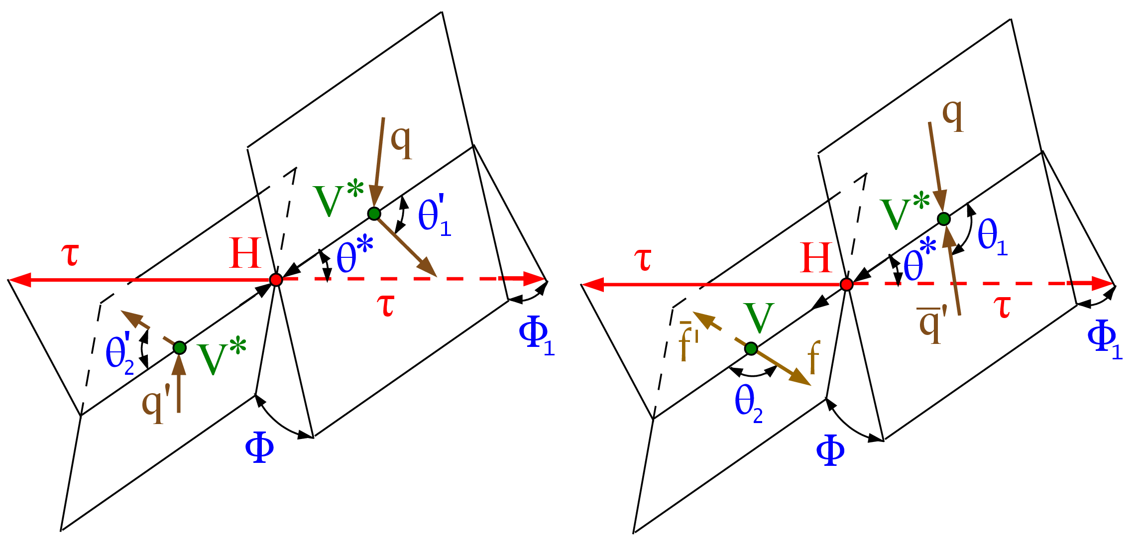
Figure 1:
Illustrations of H production in VBF ($\mathrm{q} {\mathrm{q} ^\prime}\to \mathrm{q} {\mathrm{q} ^\prime} \mathrm{H} $) (left) and VH ($\mathrm{q} \mathrm{\bar{q}} ^\prime \to \mathrm {V}^*\to \mathrm {V}\mathrm{H} \to \mathrm{q} {\mathrm{q} ^\prime} \mathrm{H} $) (right) in the rest frame of the H. The decay $\mathrm{H} \to \tau \tau $ is shown without illustrating the further decay chain. The incoming partons and fermions in the V decay are shown in brown and the intermediate or final-state particles are shown in red and green. The angles characterizing kinematic distributions are shown in blue and are defined in the respective rest frames [32,34]. The illustration for H production via ggH in association with two jets is identical to the VBF diagram, except with V=g. |
png pdf |
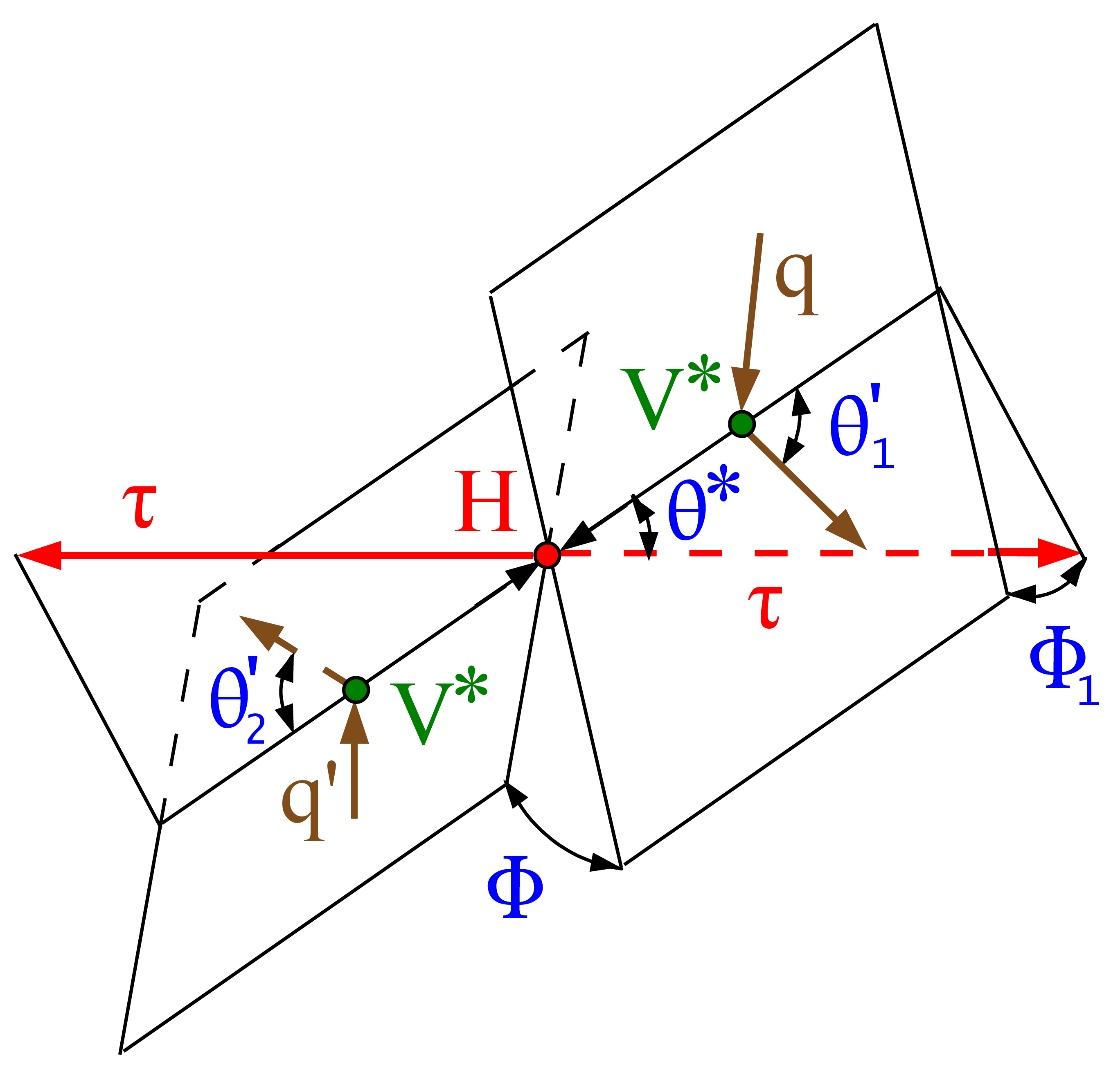
Figure 1-a:
Illustration of H production in VBF ($\mathrm{q} {\mathrm{q} ^\prime}\to \mathrm{q} {\mathrm{q} ^\prime} \mathrm{H} $) in the rest frame of the H. The decay $\mathrm{H} \to \tau \tau $ is shown without illustrating the further decay chain. The incoming and outgoing partons are shown in brown and the intermediate or final-state particles are shown in red and green. The angles characterizing kinematic distributions are shown in blue and are defined in the respective rest frames [32,34]. The illustration for H production via ggH in association with two jets is identical to this diagram, except with V=g. |
png pdf |
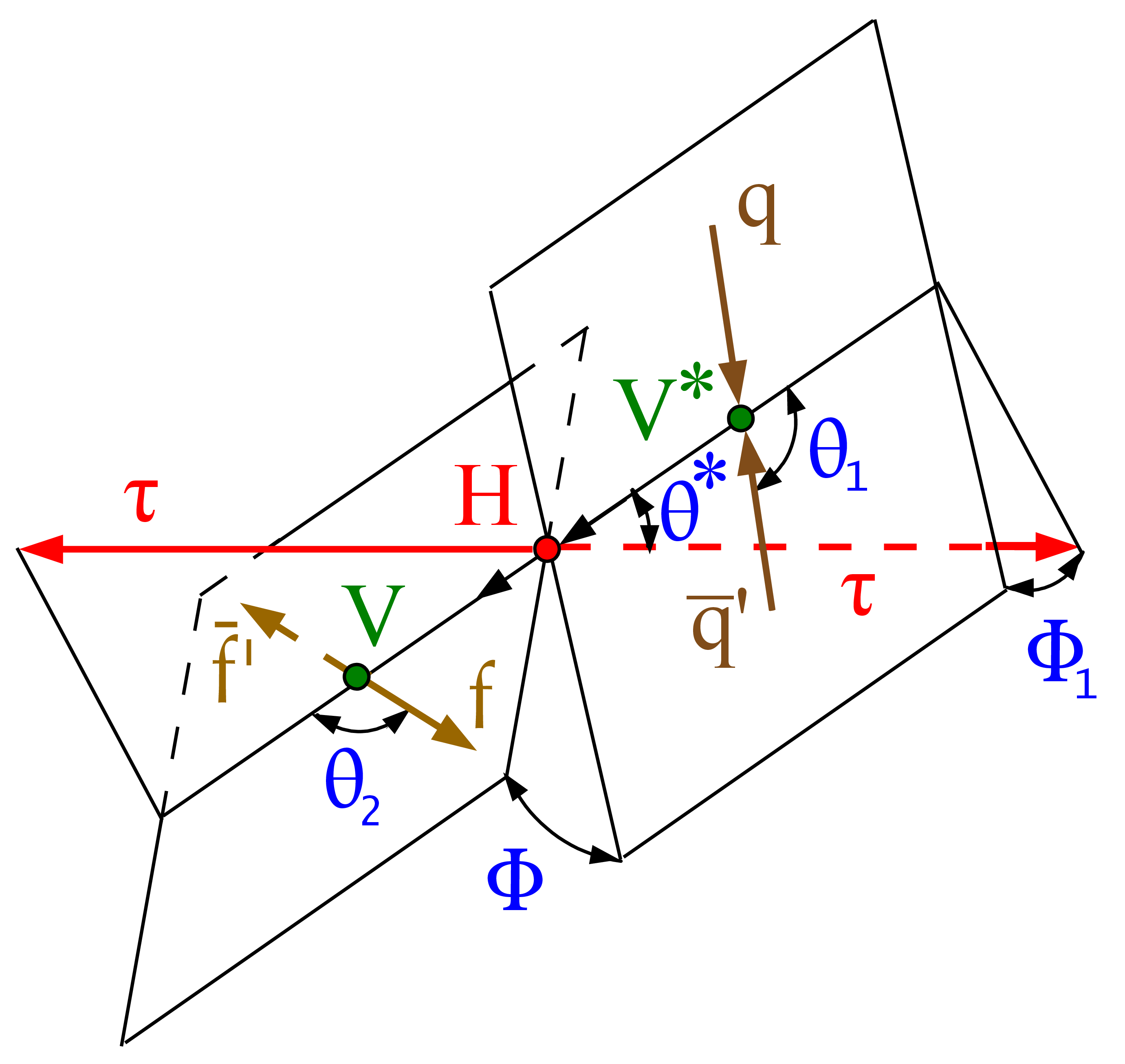
Figure 1-b:
Illustration of H production in VH ($\mathrm{q} \mathrm{\bar{q}} ^\prime \to \mathrm {V}^*\to \mathrm {V}\mathrm{H} \to \mathrm{q} {\mathrm{q} ^\prime} \mathrm{H} $) in the rest frame of the H. The decay $\mathrm{H} \to \tau \tau $ is shown without illustrating the further decay chain. The incoming partons and fermions in the V decay are shown in brown and the intermediate or final-state particles are shown in red and green. The angles characterizing kinematic distributions are shown in blue and are defined in the respective rest frames [32,34]. |

png pdf |
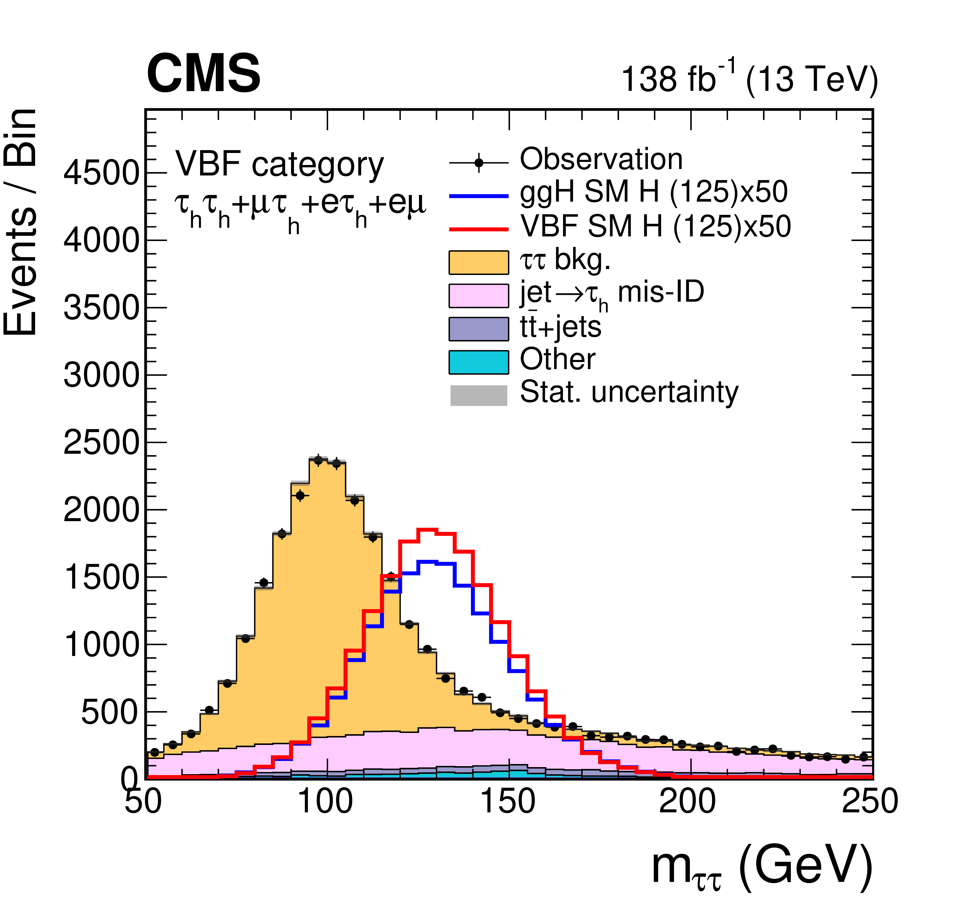
Figure 2:
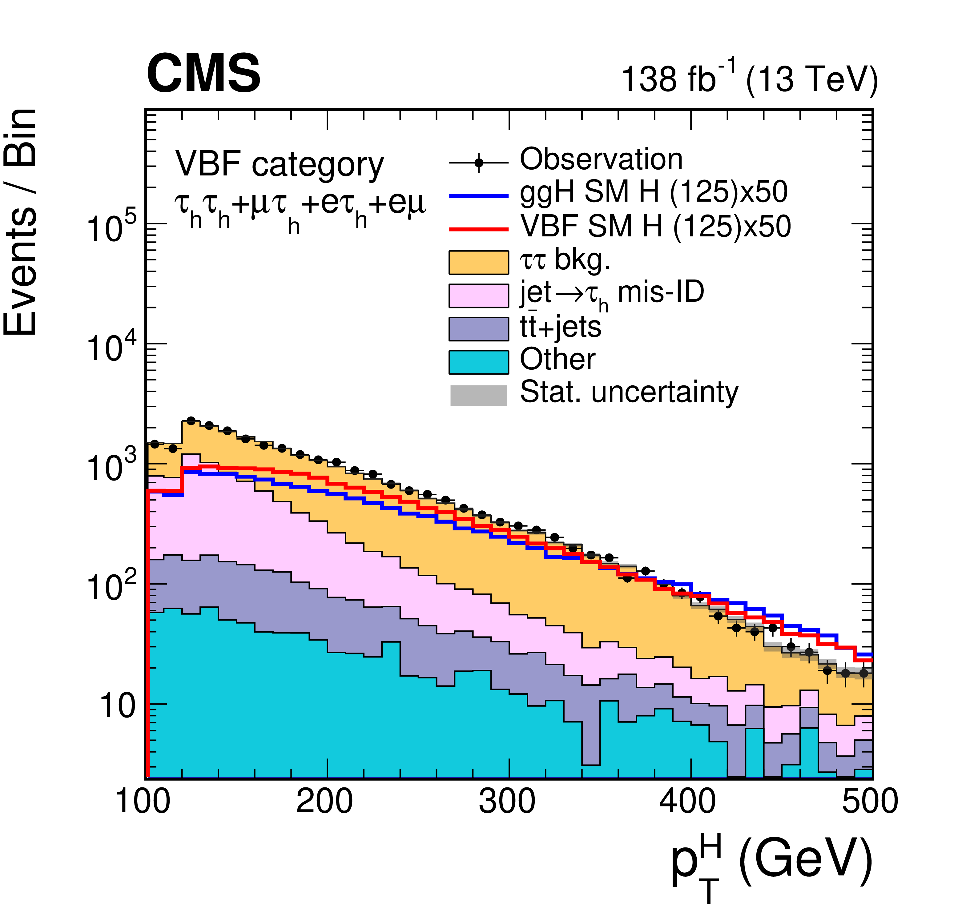
The ${m_{\tau \tau}}$ (left) and ${p_{\mathrm {T}}}$ (right) distributions for H candidate di-$\tau$ lepton pairs in the VBF category. All events selected in the e$ \mu $, e$ {\tau _\mathrm {h}} $, $\mu {\tau _\mathrm {h}} $, and $ {\tau _\mathrm {h}} {\tau _\mathrm {h}} $ final states are included. The yields of the H processes are scaled to match 50 times the SM predictions. Only statistical uncertainties are shown. |
png pdf |
Figure 2-a:
The ${m_{\tau \tau}}$ distribution for H candidate di-$\tau$ lepton pairs in the VBF category. All events selected in the e$ \mu $, e$ {\tau _\mathrm {h}} $, $\mu {\tau _\mathrm {h}} $, and $ {\tau _\mathrm {h}} {\tau _\mathrm {h}} $ final states are included. The yields of the H processes are scaled to match 50 times the SM predictions. Only statistical uncertainties are shown. |
png pdf |
Figure 2-b:
The ${p_{\mathrm {T}}}$ distribution for H candidate di-$\tau$ lepton pairs in the VBF category. All events selected in the e$ \mu $, e$ {\tau _\mathrm {h}} $, $\mu {\tau _\mathrm {h}} $, and $ {\tau _\mathrm {h}} {\tau _\mathrm {h}} $ final states are included. The yields of the H processes are scaled to match 50 times the SM predictions. Only statistical uncertainties are shown. |
png pdf |
Figure 3:
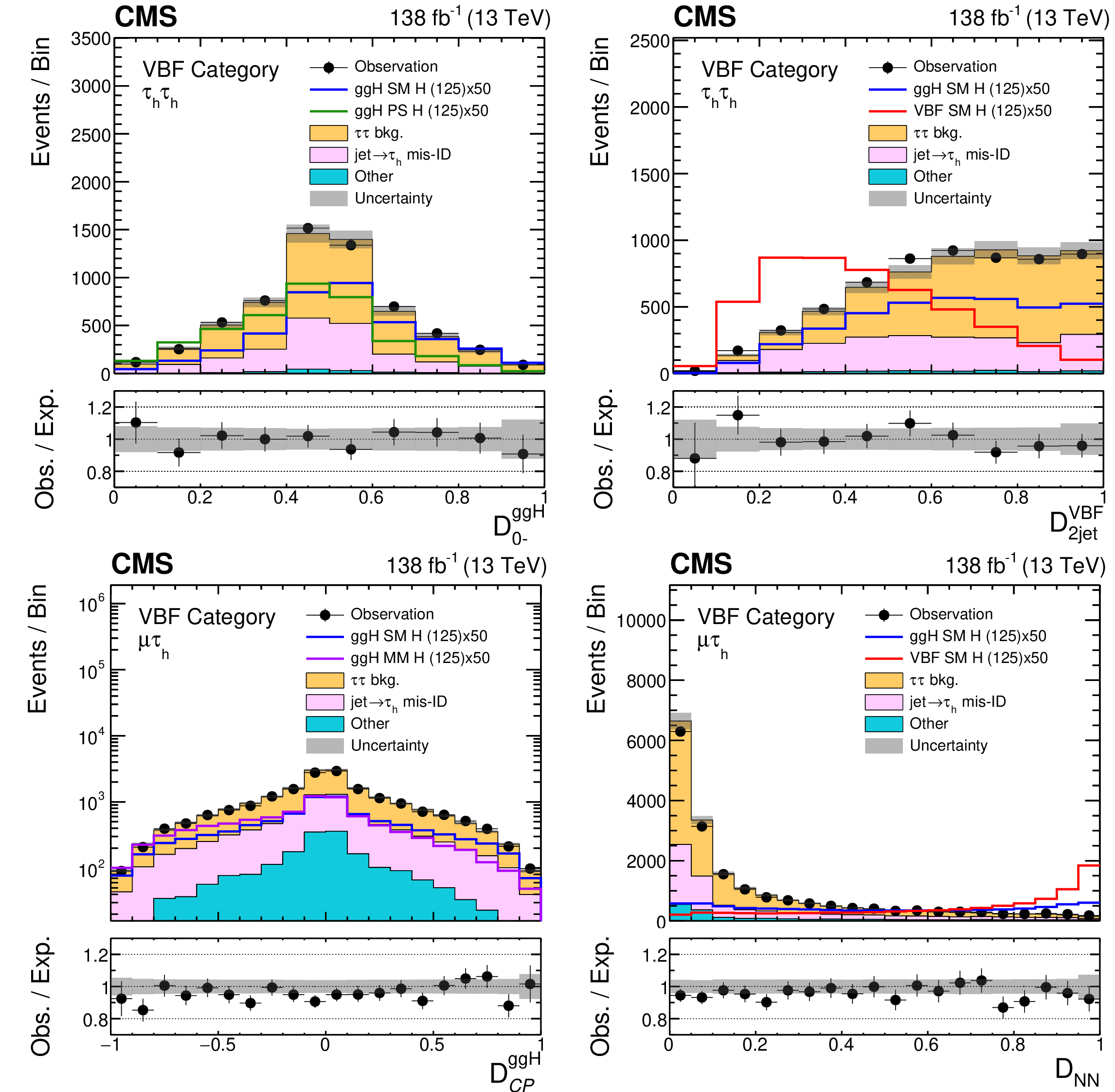
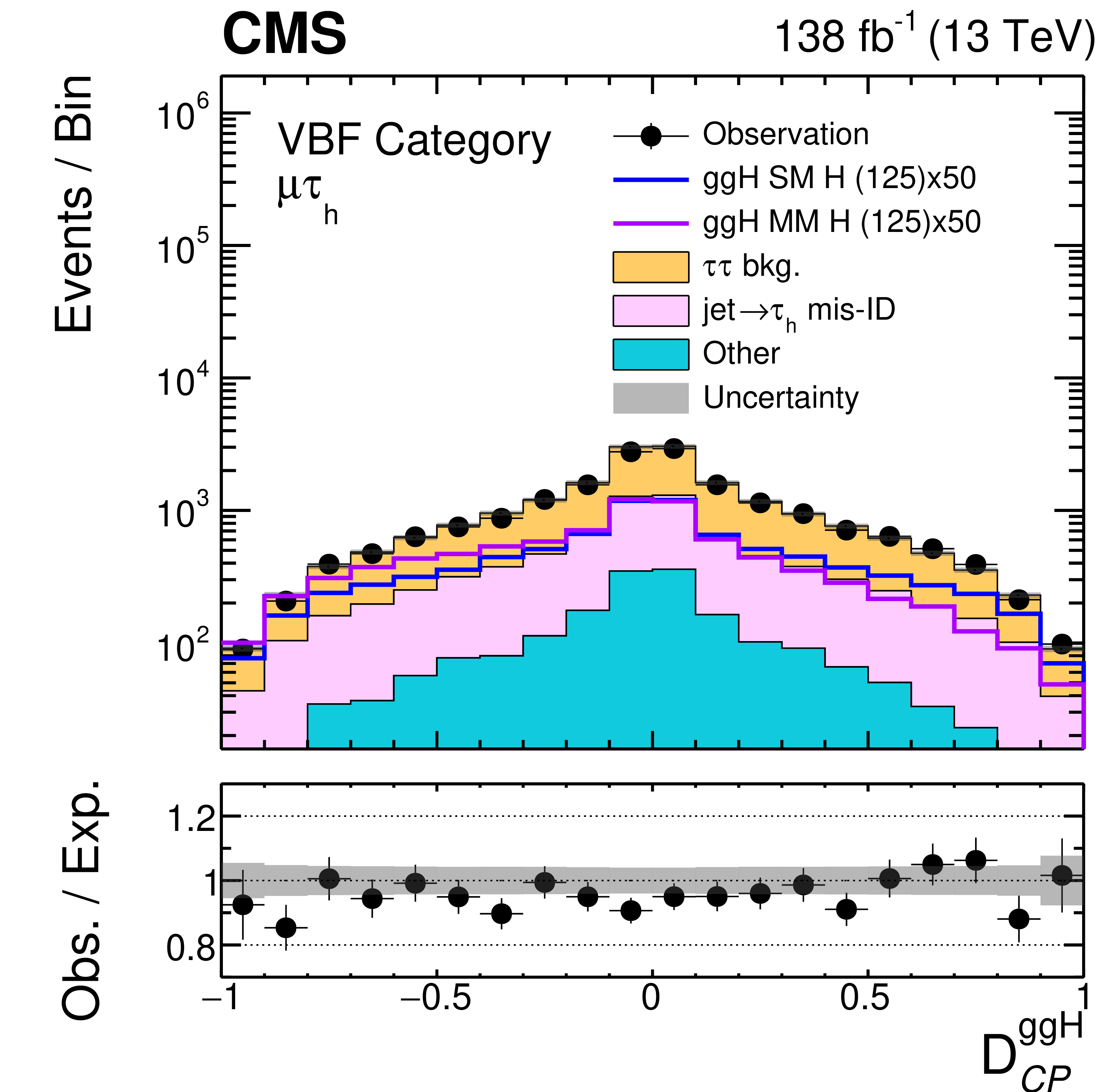
Examples of data and signal and background predictions for MELA and neural network discriminants in the $ {\tau _\mathrm {h}} {\tau _\mathrm {h}} $ and $\mu {\tau _\mathrm {h}} $ channels. Events passing the selections outlined in Section 6 and allocated to the VBF category are included. The yields of the H processes are scaled to match 50 times the SM predictions. The uncertainty band includes statistical uncertainties and systematic uncertainties that affect the normalization of the background distribution. The expectation in the ratio panel is the sum of the estimated backgrounds and the SM H signal. For the ${\mathcal {D}_{0-}^{\mathrm{g} \mathrm{g} \mathrm{H}}}$ discriminant the distribution expected for a pseudoscalar H hypothesis (labeled "PS" in the legend) is overlaid to be compared to the SM signal. Similarly, for the ${\mathcal {D}_{\text{CP}}^{\mathrm{g} \mathrm{g} \mathrm{H}}}$ discriminant the distribution for a CP-violating scenario with the maximum-mixing between CP-even and CP-odd couplings (labeled "MM" in the legend) is shown. |
png pdf |
Figure 3-a:
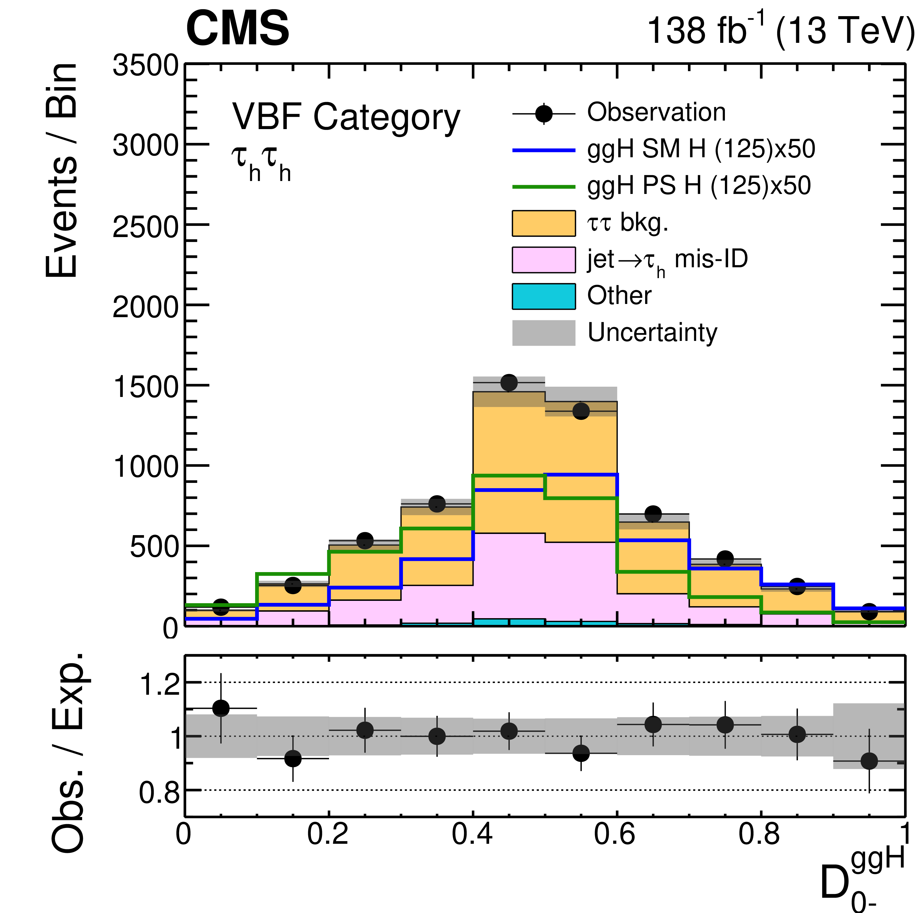
Data and signal and background predictions for the ${\mathcal {D}_{0-}^{\mathrm{g} \mathrm{g} \mathrm{H}}}$ discriminant in the $ {\tau _\mathrm {h}} {\tau _\mathrm {h}} $ and $\mu {\tau _\mathrm {h}} $ channels. Events passing the selections outlined in Section 6 and allocated to the VBF category are included. The yields of the H processes are scaled to match 50 times the SM predictions. The uncertainty band includes statistical uncertainties and systematic uncertainties that affect the normalization of the background distribution. The expectation in the ratio panel is the sum of the estimated backgrounds and the SM H signal. The distribution expected for a pseudoscalar H hypothesis (labeled "PS" in the legend) is overlaid to be compared to the SM signal. |
png pdf |
Figure 3-b:
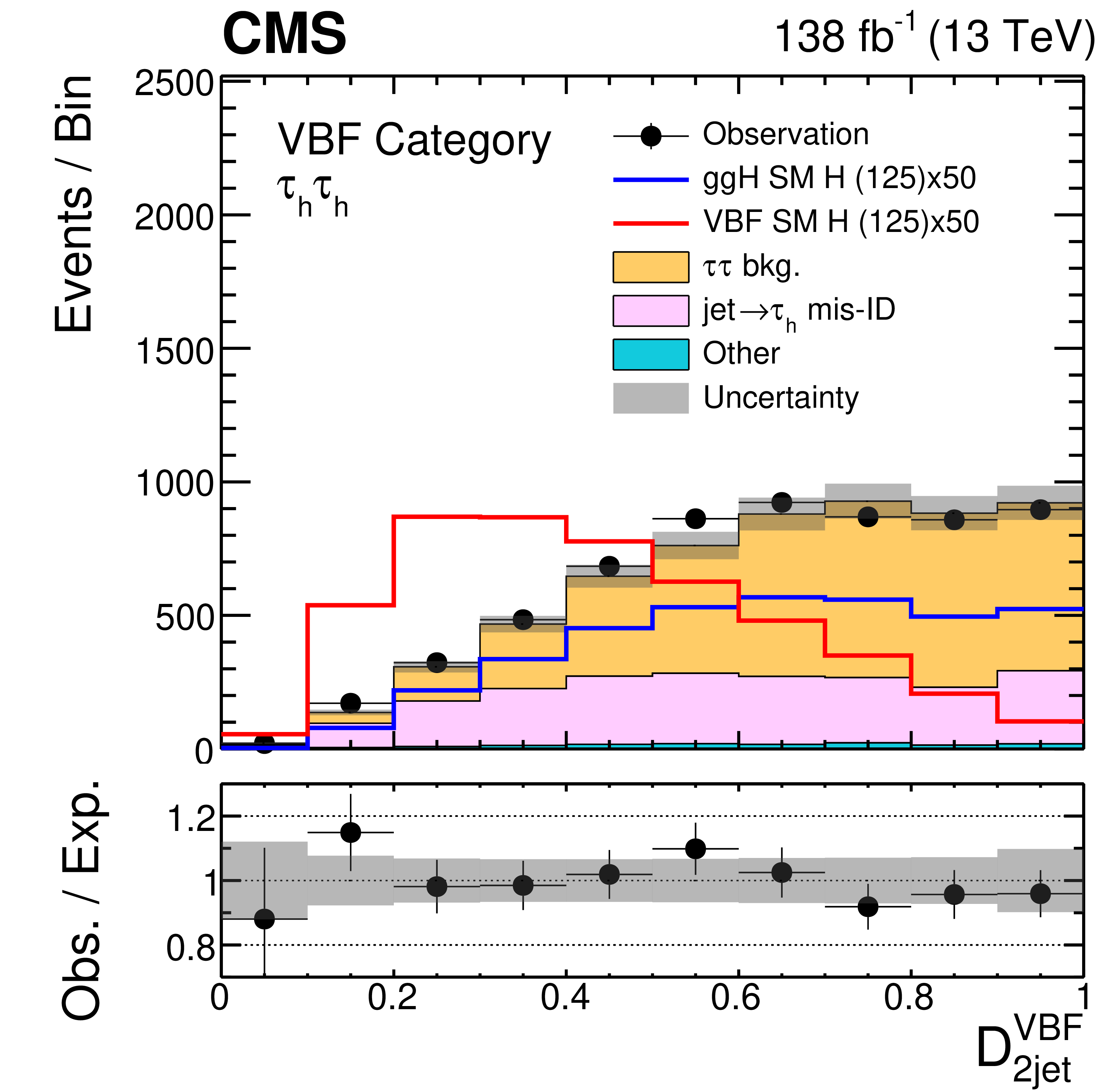
Data and signal and background predictions for the ${\mathcal {D}_\mathrm {2jet}^\mathrm {VBF}}$ discriminant in the $ {\tau _\mathrm {h}} {\tau _\mathrm {h}} $ and $\mu {\tau _\mathrm {h}} $ channels. Events passing the selections outlined in Section 6 and allocated to the VBF category are included. The yields of the H processes are scaled to match 50 times the SM predictions. The uncertainty band includes statistical uncertainties and systematic uncertainties that affect the normalization of the background distribution. The expectation in the ratio panel is the sum of the estimated backgrounds and the SM H signal. |
png pdf |
Figure 3-c:
Data and signal and background predictions for the ${\mathcal {D}_{\text{CP}}^{\mathrm{g} \mathrm{g} \mathrm{H}}}$ discriminant in the $ {\tau _\mathrm {h}} {\tau _\mathrm {h}} $ and $\mu {\tau _\mathrm {h}} $ channels. Events passing the selections outlined in Section 6 and allocated to the VBF category are included. The yields of the H processes are scaled to match 50 times the SM predictions. The uncertainty band includes statistical uncertainties and systematic uncertainties that affect the normalization of the background distribution. The expectation in the ratio panel is the sum of the estimated backgrounds and the SM H signal. The distribution for a CP-violating scenario with the maximum-mixing between CP-even and CP-odd couplings (labeled "MM" in the legend) is shown. |

png pdf |
Figure 3-d:
Data and signal and background predictions for the ${\mathcal {D}_\mathrm {NN}}$ discriminant in the $ {\tau _\mathrm {h}} {\tau _\mathrm {h}} $ and $\mu {\tau _\mathrm {h}} $ channels. Events passing the selections outlined in Section 6 and allocated to the VBF category are included. The yields of the H processes are scaled to match 50 times the SM predictions. The uncertainty band includes statistical uncertainties and systematic uncertainties that affect the normalization of the background distribution. The expectation in the ratio panel is the sum of the estimated backgrounds and the SM H signal. |
png pdf |
Figure 4:
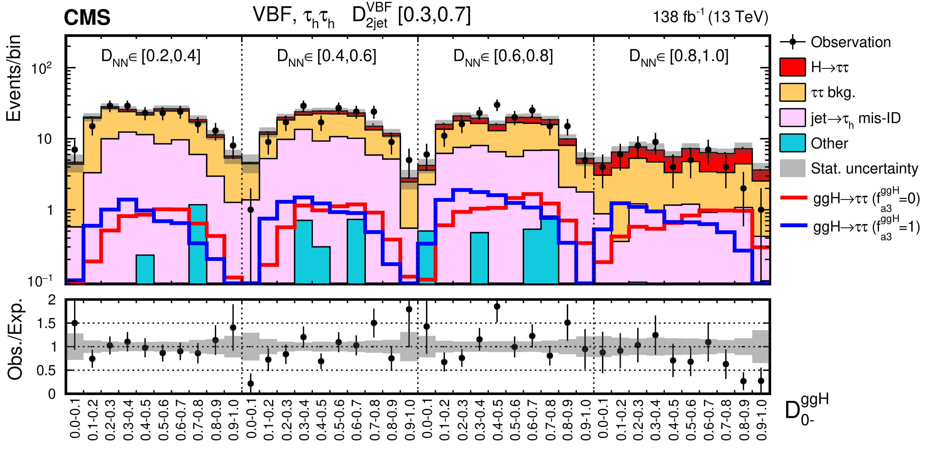
The observed and predicted 2D distribution of (${\mathcal {D}_{0-}^{\mathrm{g} \mathrm{g} \mathrm{H}}}$, ${\mathcal {D}_\mathrm {NN}}$) before the fit to data in the most sensitive VBF category region with 0.3 $ < {\mathcal {D}_\mathrm {2jet}^\mathrm {VBF}} < $ 0.7 in the $ {\tau _\mathrm {h}} {\tau _\mathrm {h}} $ channel. The total H signal, including VBF, ggH, and VH processes, is shown stacked on top of the background in the solid red histogram. The ggH signal for the CP-even (CP-odd) scenario is also shown overlain by the red (blue) line. Only the statistical uncertainties are included in the uncertainty band. |
png pdf |
Figure 5:
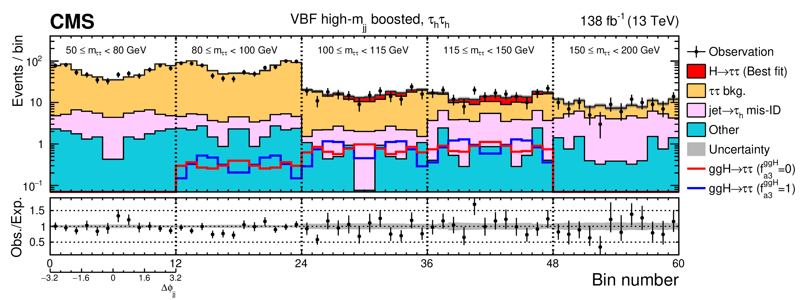
Observed and predicted 2D distributions after the fit to data in the VBF high-$ {m_{\mathrm {jj}}}$ boosted category in the $ {\tau _\mathrm {h}} {\tau _\mathrm {h}} $ channel. The total H signal, including VBF, ggH, and VH processes, is shown stacked on top of the background in the solid red histogram. The ggH signal for the CP-even (CP-odd) scenario is also shown overlain by the red (blue) line. The uncertainty band accounts for all sources of systematic uncertainty in the signal and background predictions. The expectation in the ratio panel is the sum of the estimated backgrounds and the best fit signal. |
png pdf |
Figure 6:
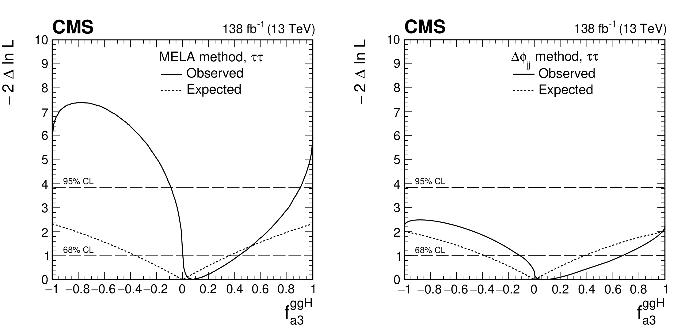
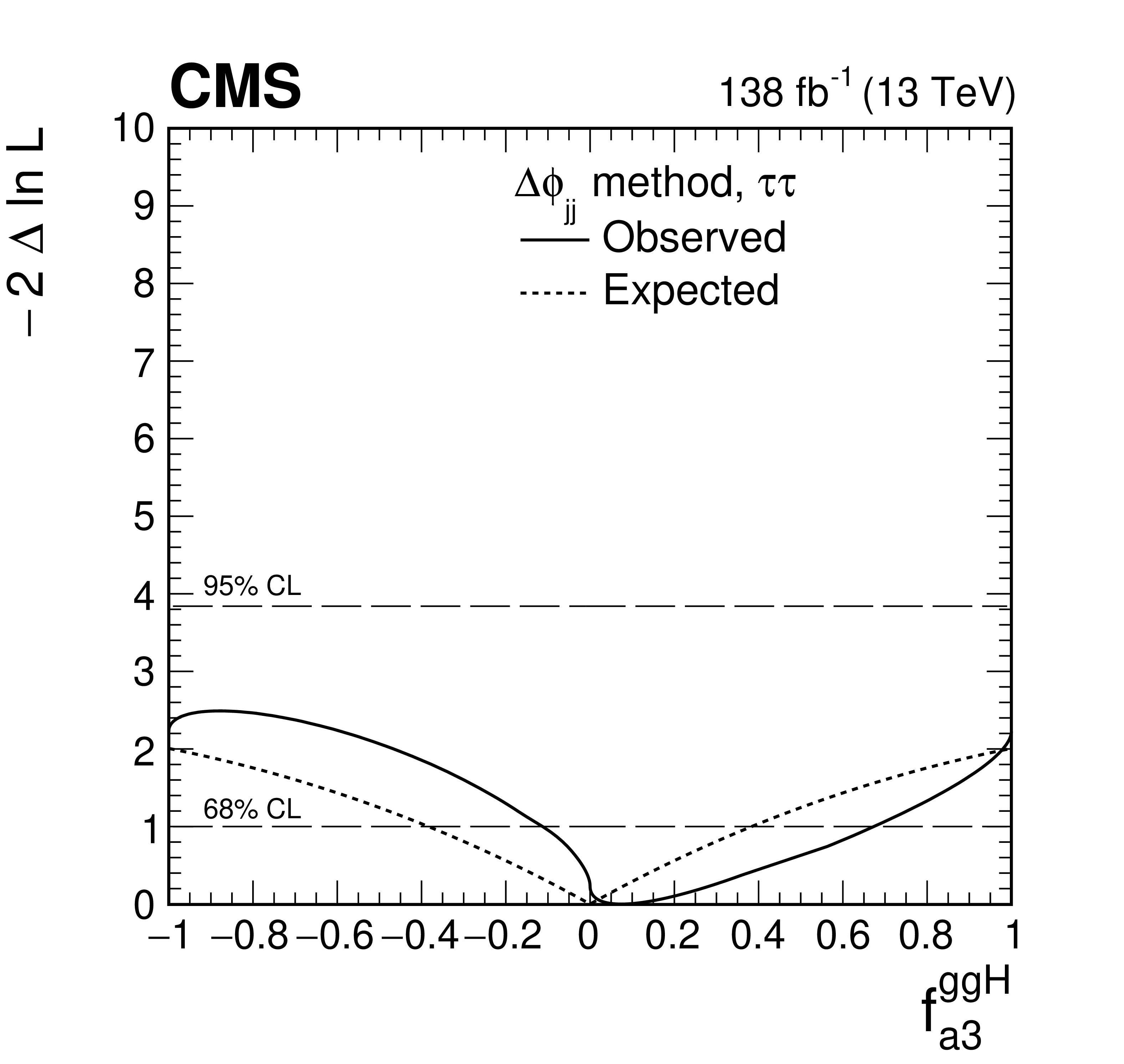
Observed (solid) and expected (dashed) likelihood scans of ${f_{a3}^{\mathrm{g} \mathrm{g} \mathrm{H}}}$ obtained with the MELA method (left) and the ${\Delta \phi _{\mathrm {jj}}}$ method used as a cross check (right). |

png pdf |
Figure 6-a:
Observed (solid) and expected (dashed) likelihood scans of ${f_{a3}^{\mathrm{g} \mathrm{g} \mathrm{H}}}$ obtained with the MELA method. |
png pdf |
Figure 6-b:
Observed (solid) and expected (dashed) likelihood scans of ${f_{a3}^{\mathrm{g} \mathrm{g} \mathrm{H}}}$ obtained with the ${\Delta \phi _{\mathrm {jj}}}$ method used as a cross check. |
png pdf |
Figure 7:
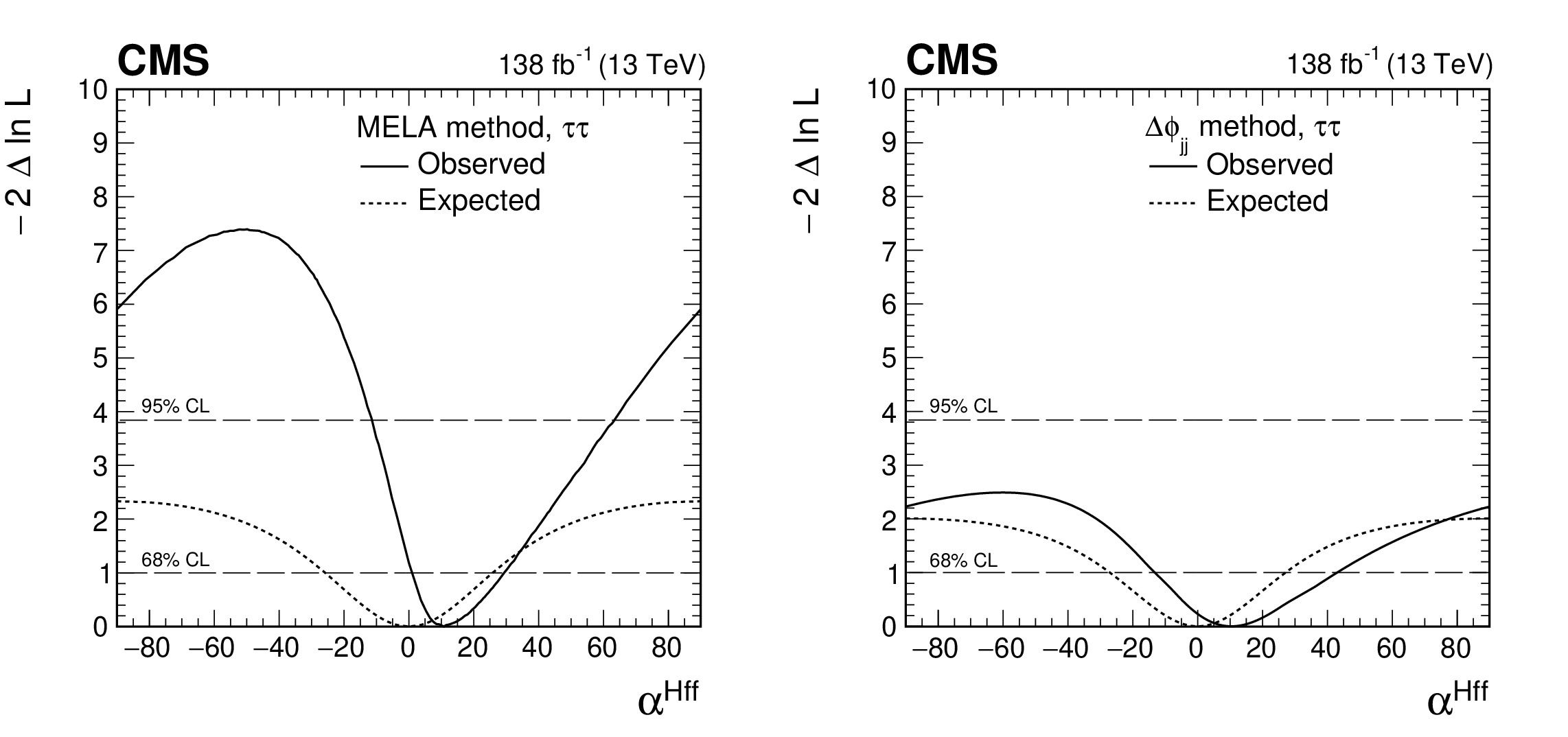
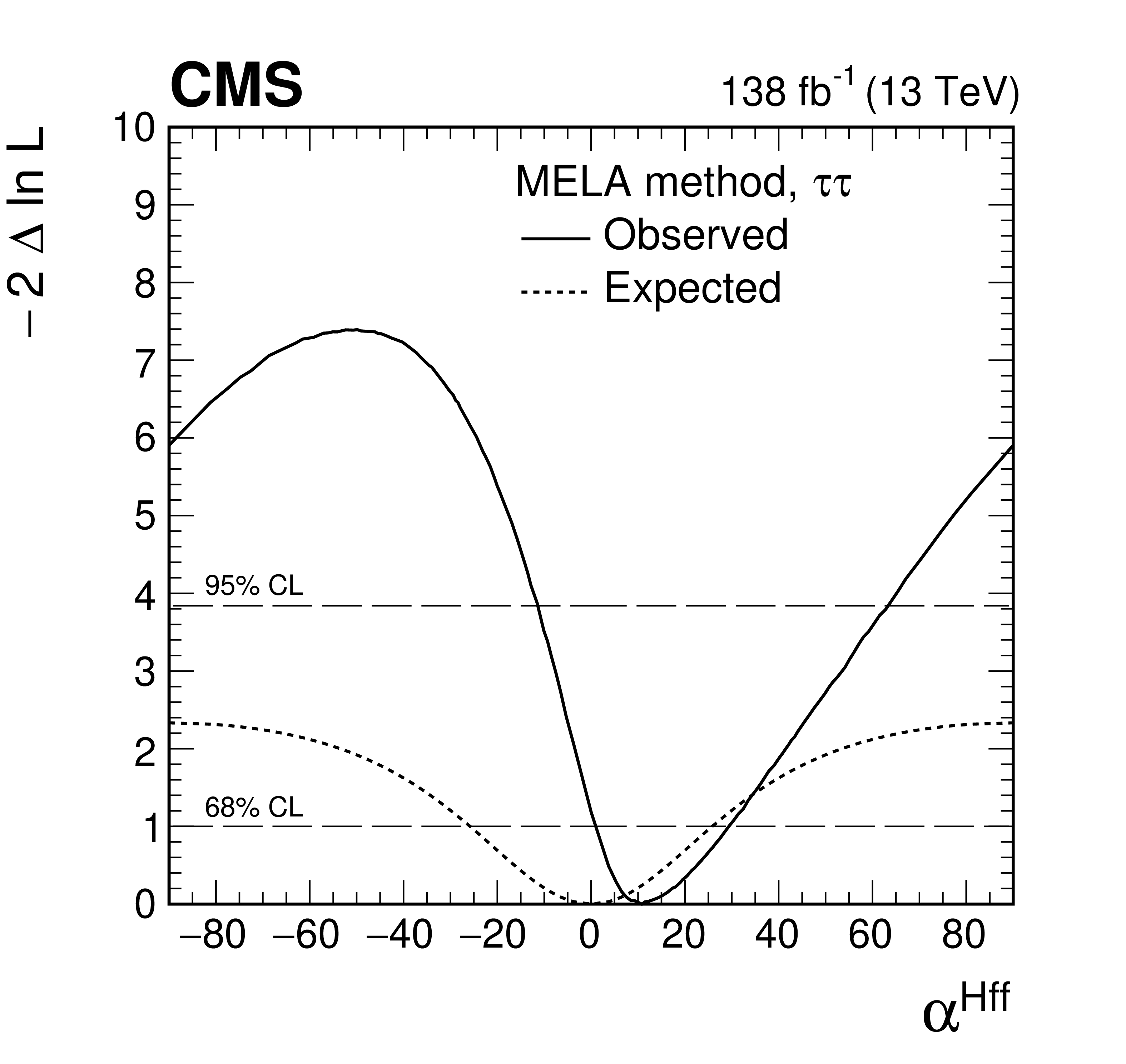
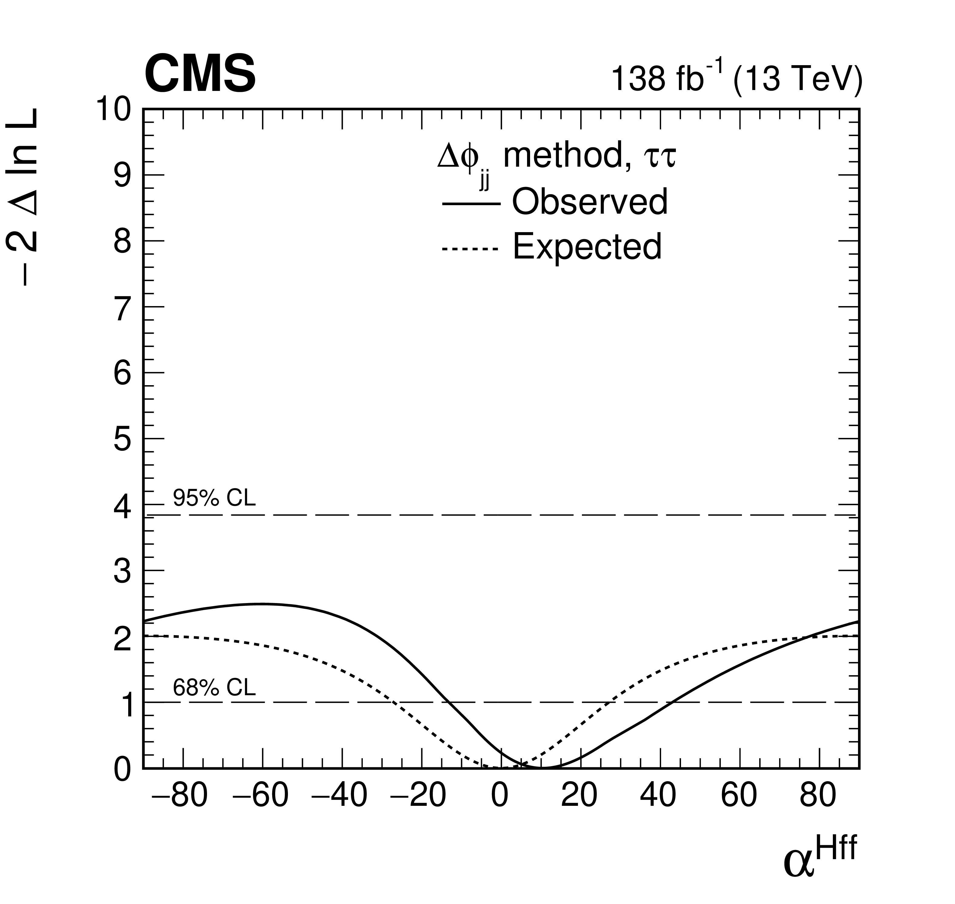
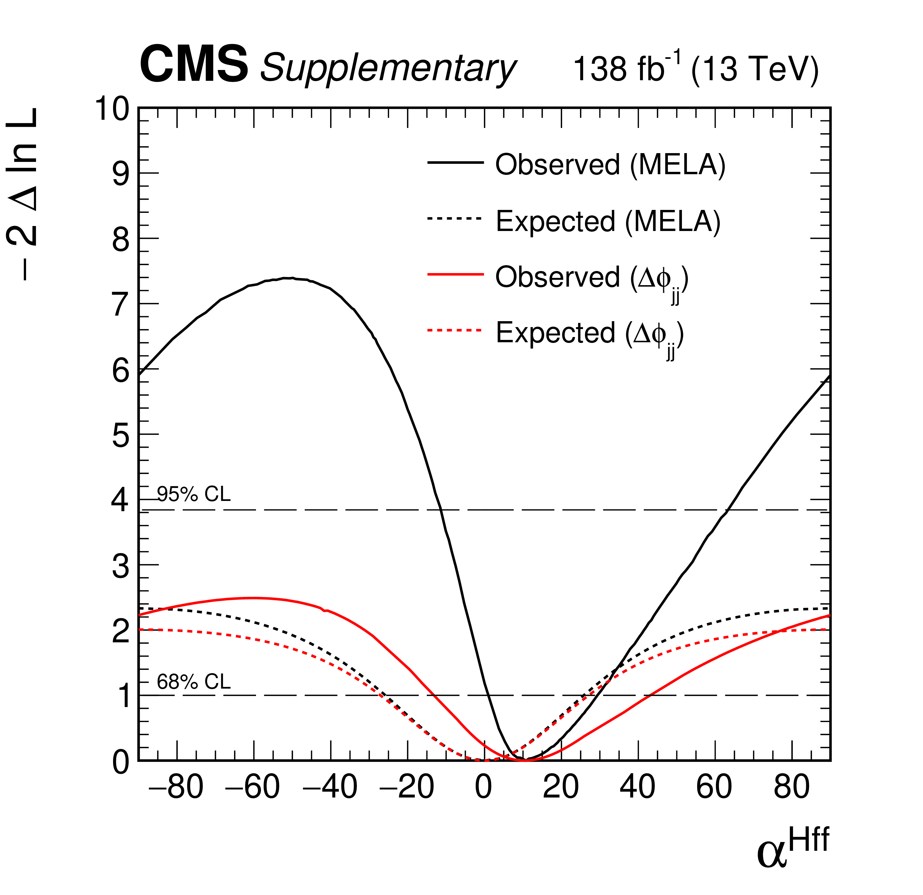
Observed (solid) and expected (dashed) likelihood scans of ${\alpha ^{\mathrm{H} \mathrm {ff}}}$ (in degrees) obtained with the MELA method (left) and the ${\Delta \phi _{\mathrm {jj}}}$ method used as a cross check (right). |
png pdf |
Figure 7-a:
Observed (solid) and expected (dashed) likelihood scans of ${\alpha ^{\mathrm{H} \mathrm {ff}}}$ (in degrees) obtained with the MELA method. |
png pdf |
Figure 7-b:
Observed (solid) and expected (dashed) likelihood scans of ${\alpha ^{\mathrm{H} \mathrm {ff}}}$ (in degrees) obtained with the ${\Delta \phi _{\mathrm {jj}}}$ method used as a cross check. |
png pdf |
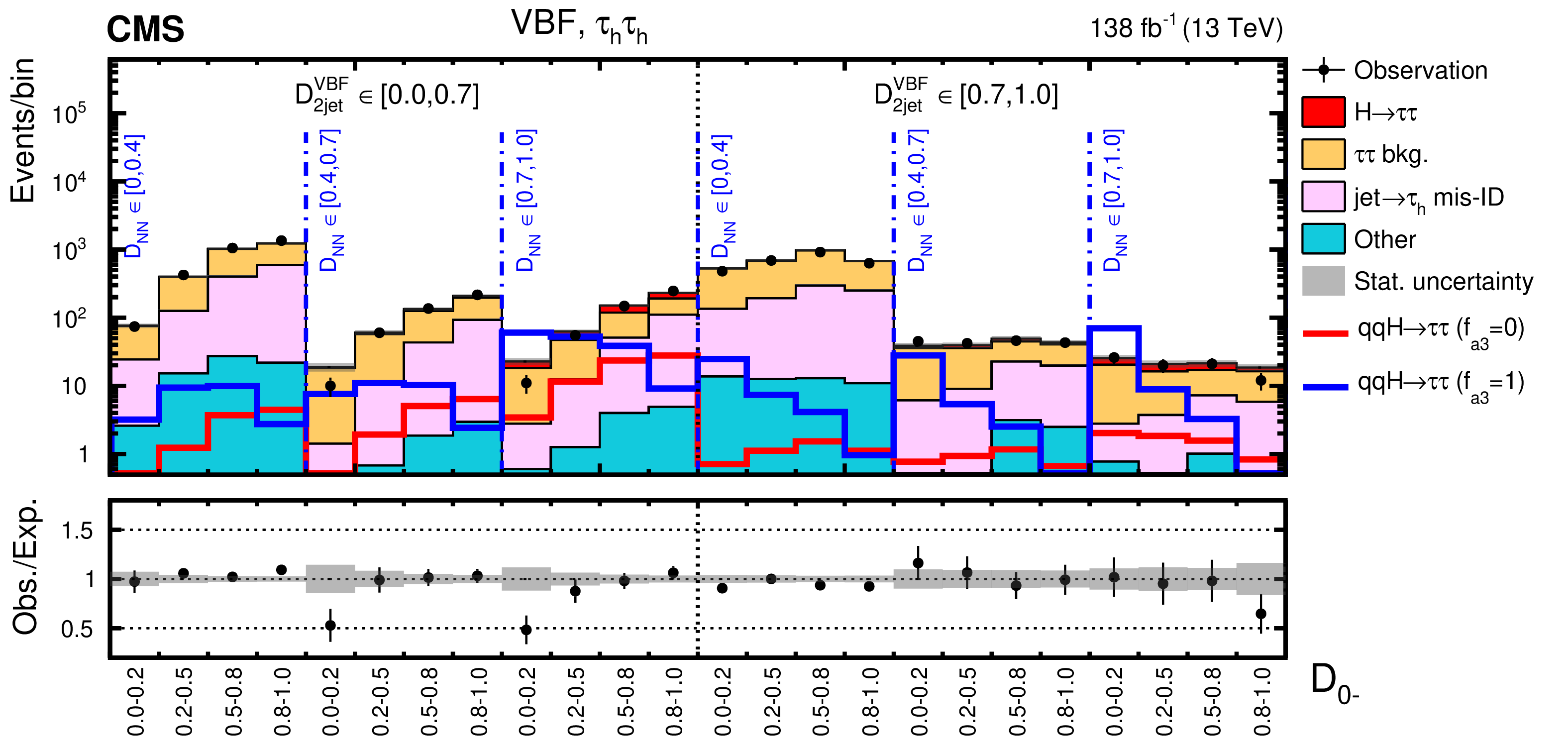
Figure 8:
The observed and predicted 3D distribution of (${\mathcal {D}_{0-}}, {\mathcal {D}_\mathrm {NN}}$, ${\mathcal {D}_\mathrm {2jet}^\mathrm {VBF}}$) before the fit to data in the $ {\tau _\mathrm {h}} {\tau _\mathrm {h}} $ channel for the most sensitive VBF category. The total H signal, including VBF, ggH, and VH processes, is shown stacked on top of the background in the solid red histogram. The VBF+ VH signal for the CP-even (CP-odd) scenario is also shown overlain by the red (blue) line. Only the statistical uncertainties are included in the uncertainty band. |
png pdf |
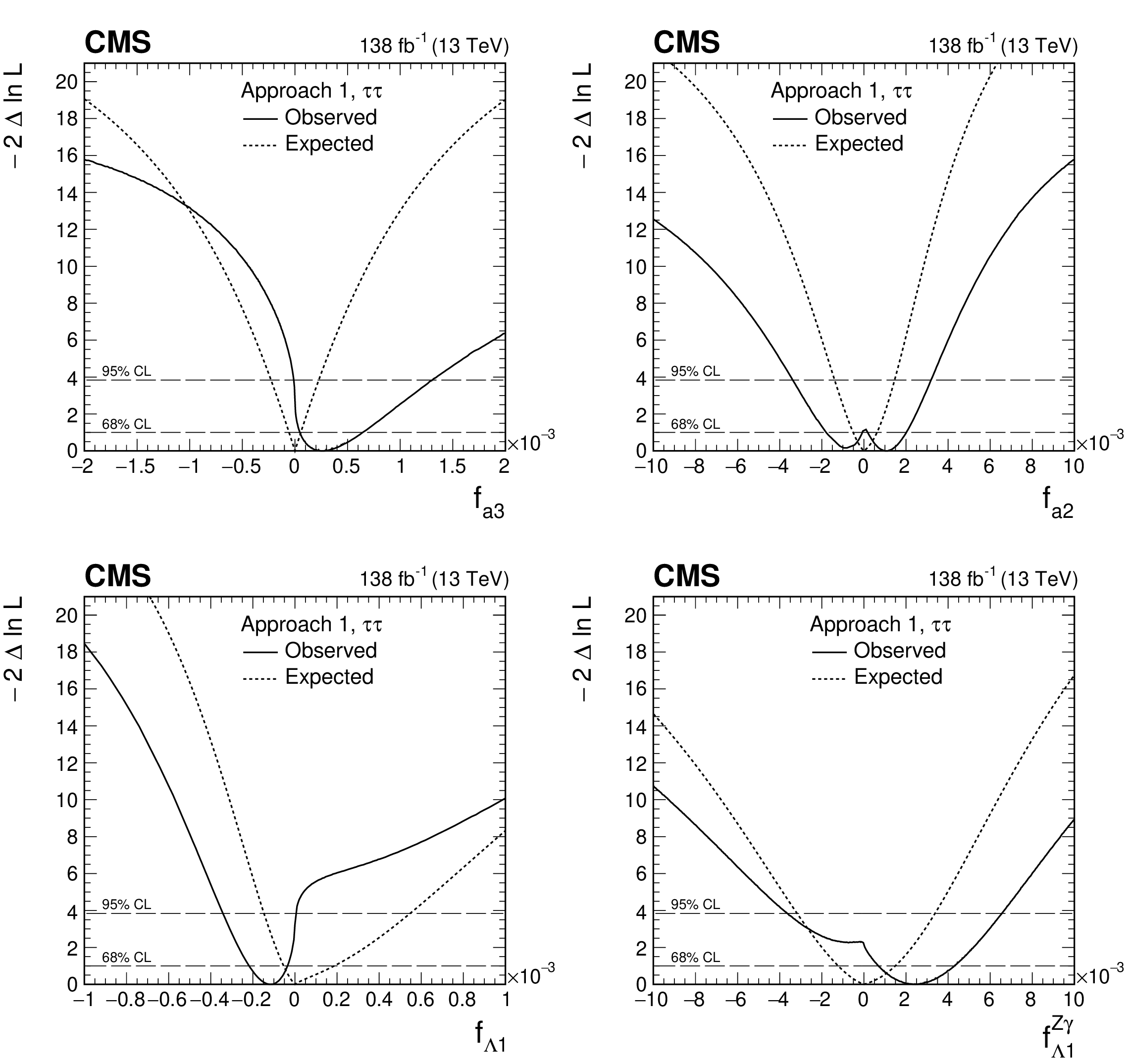
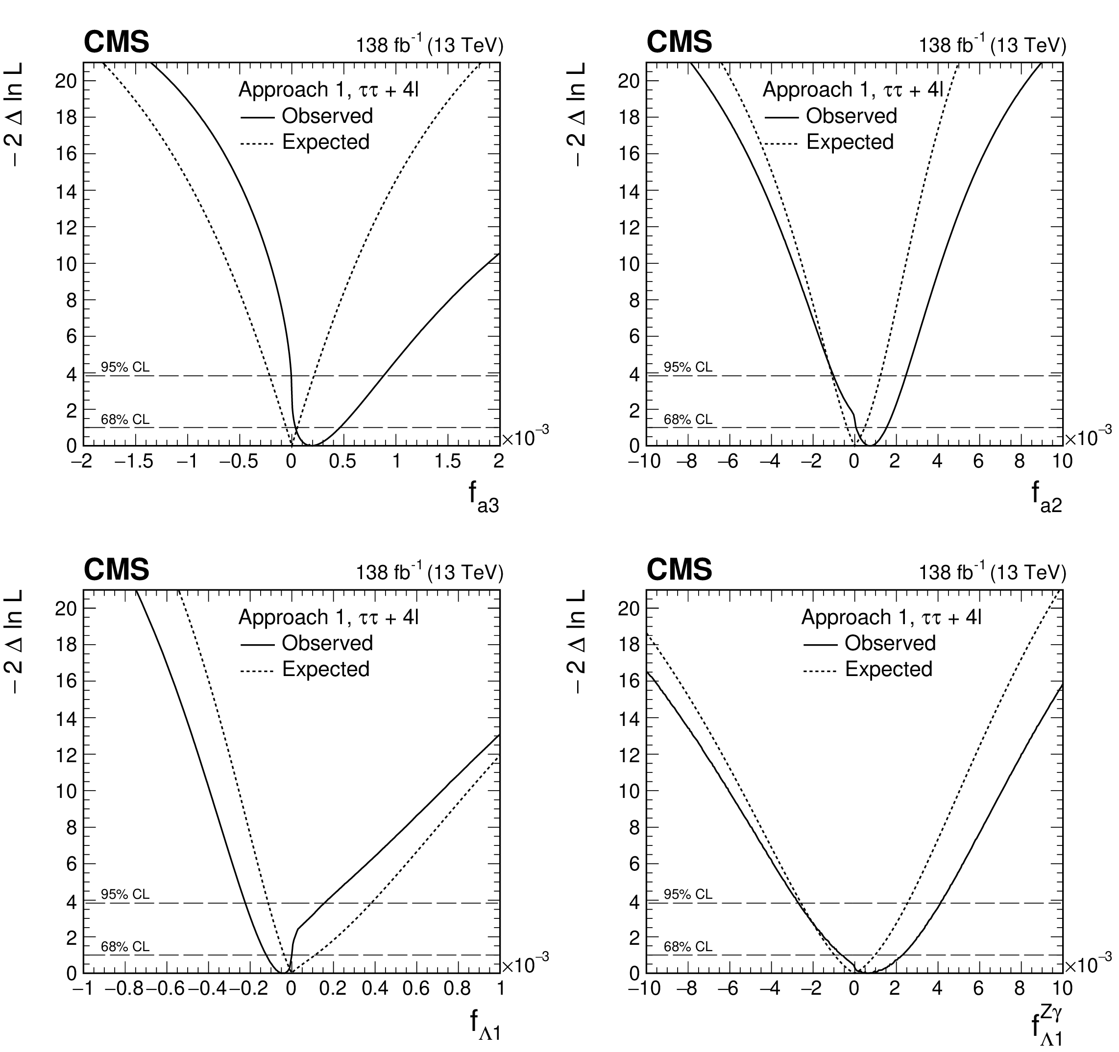
Figure 9:
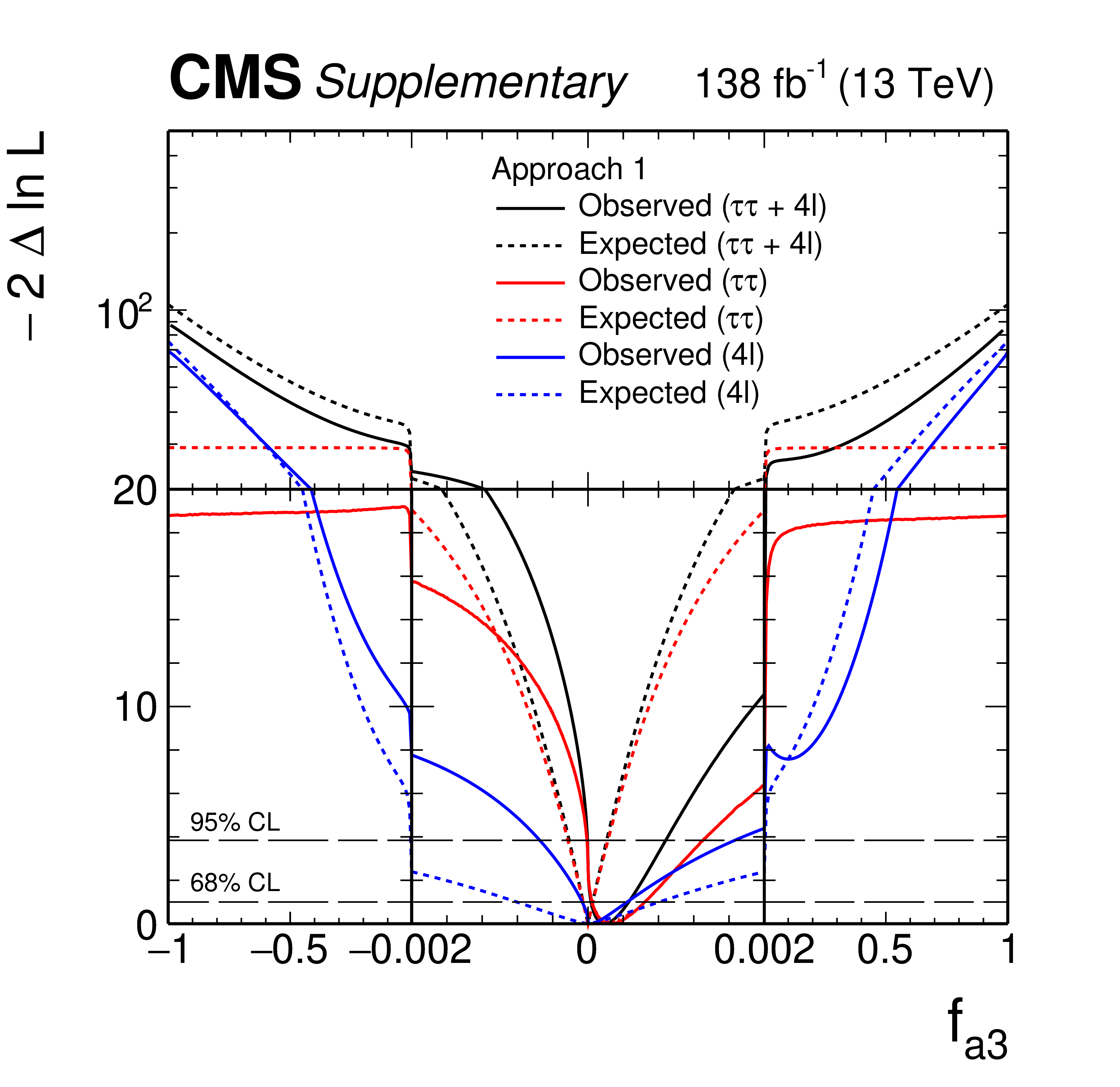
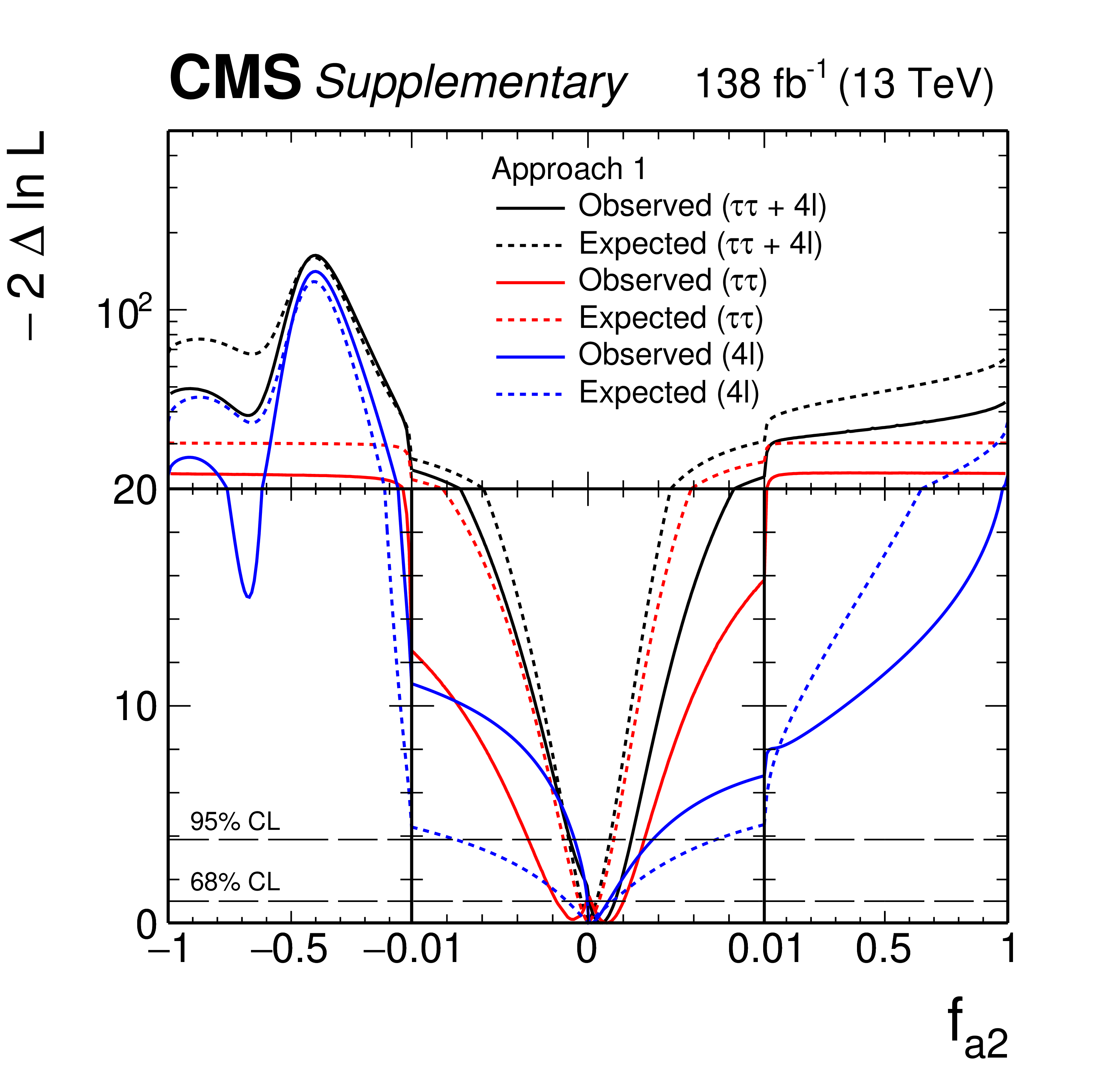
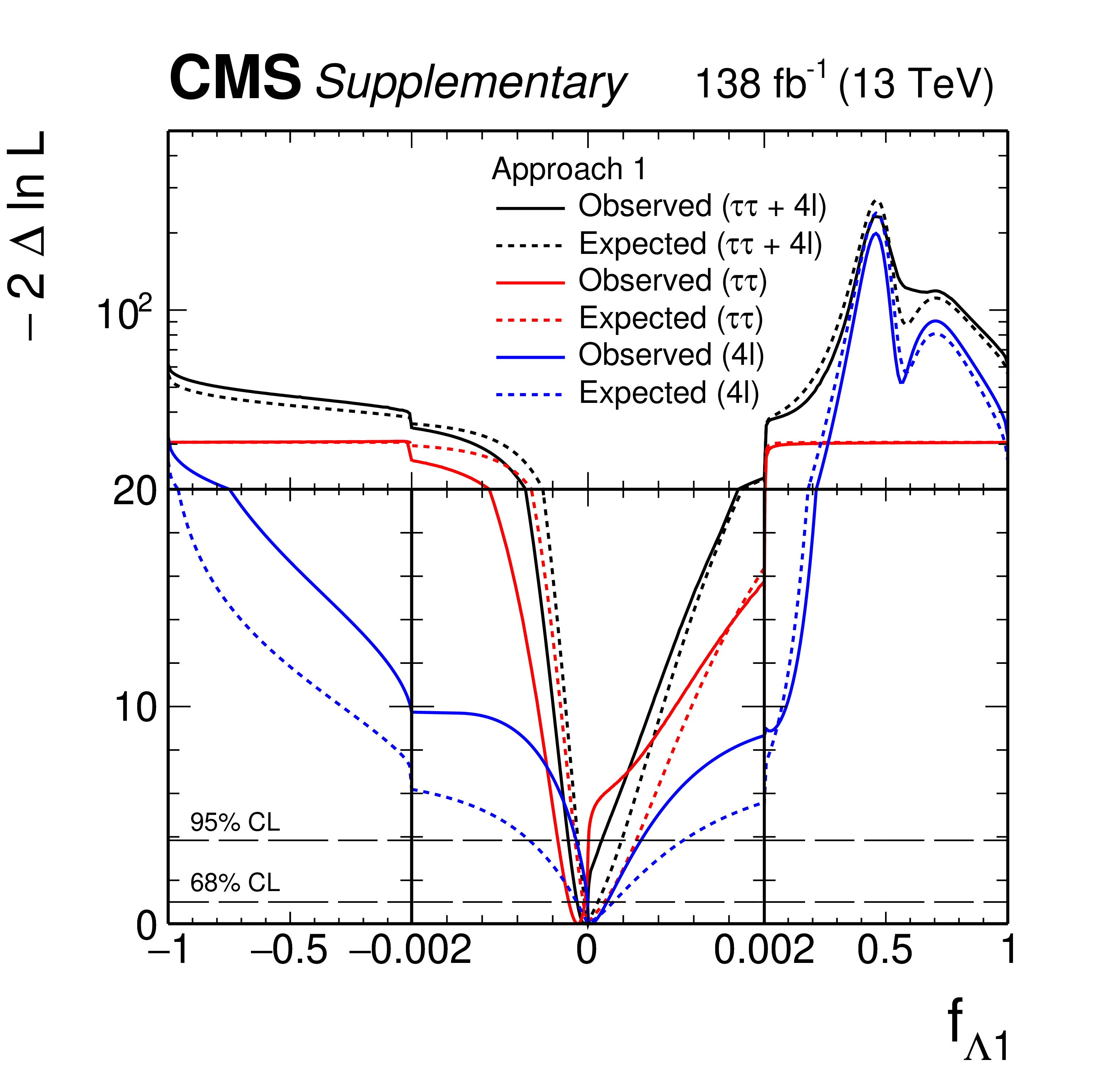
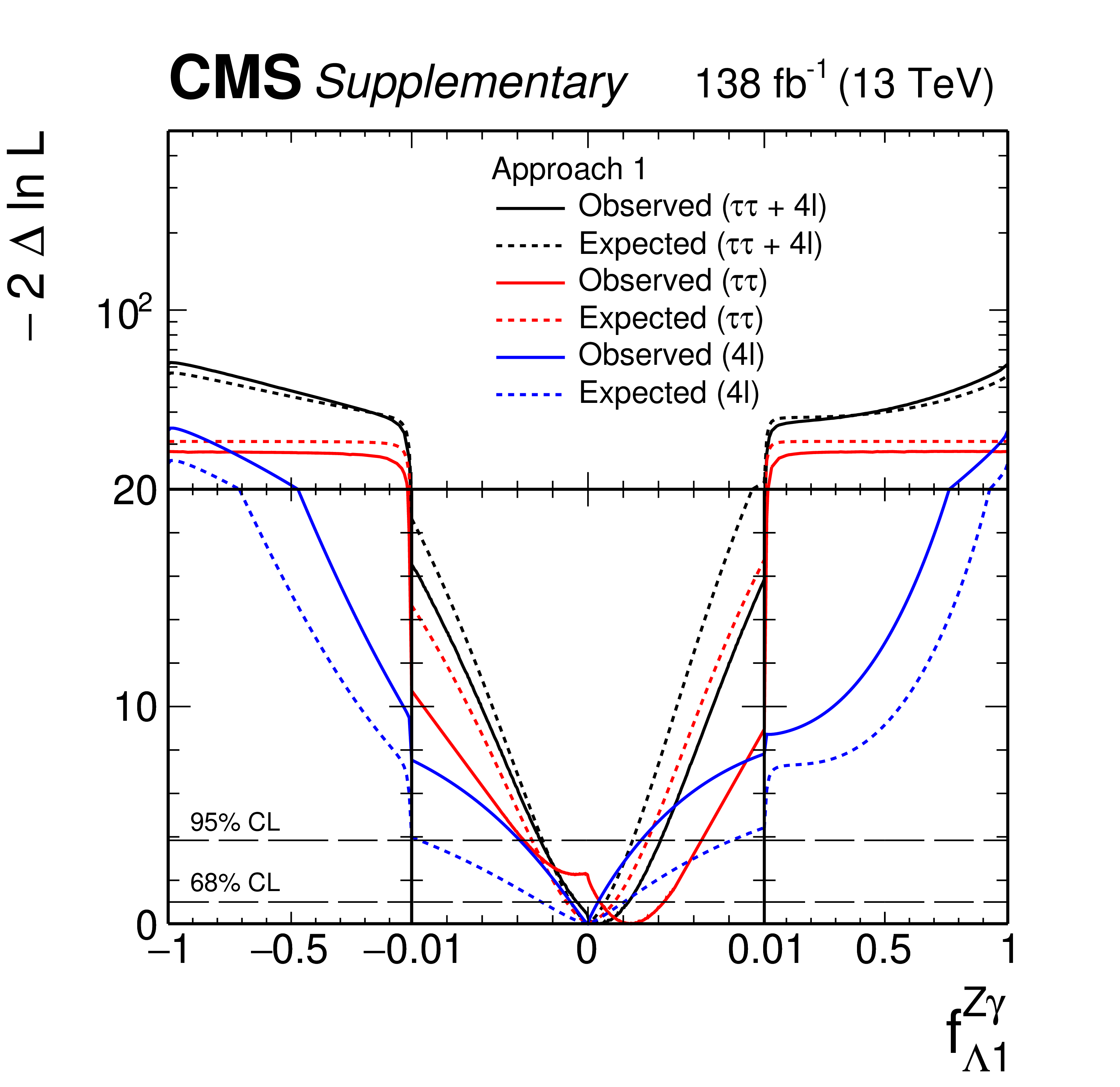
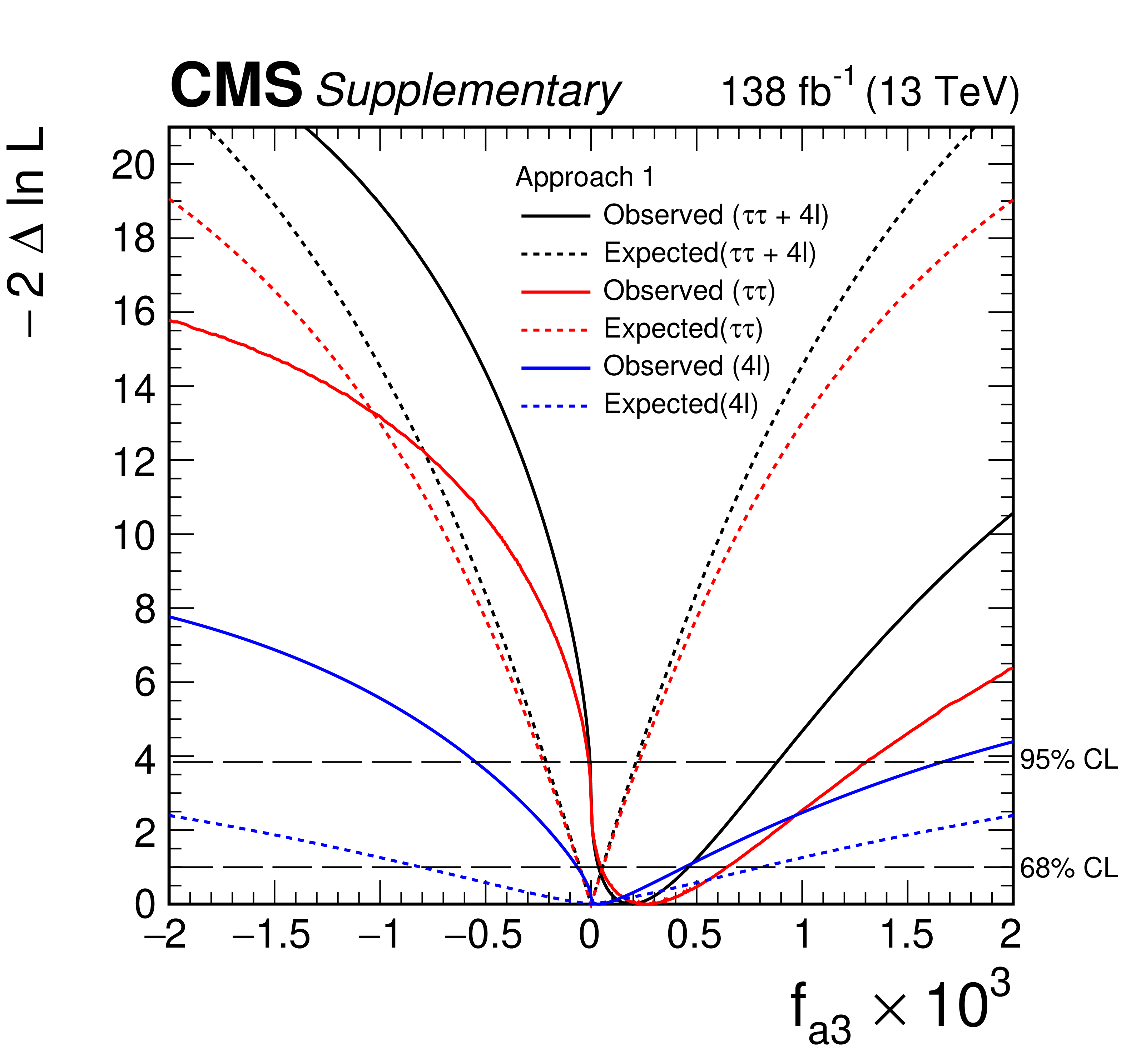
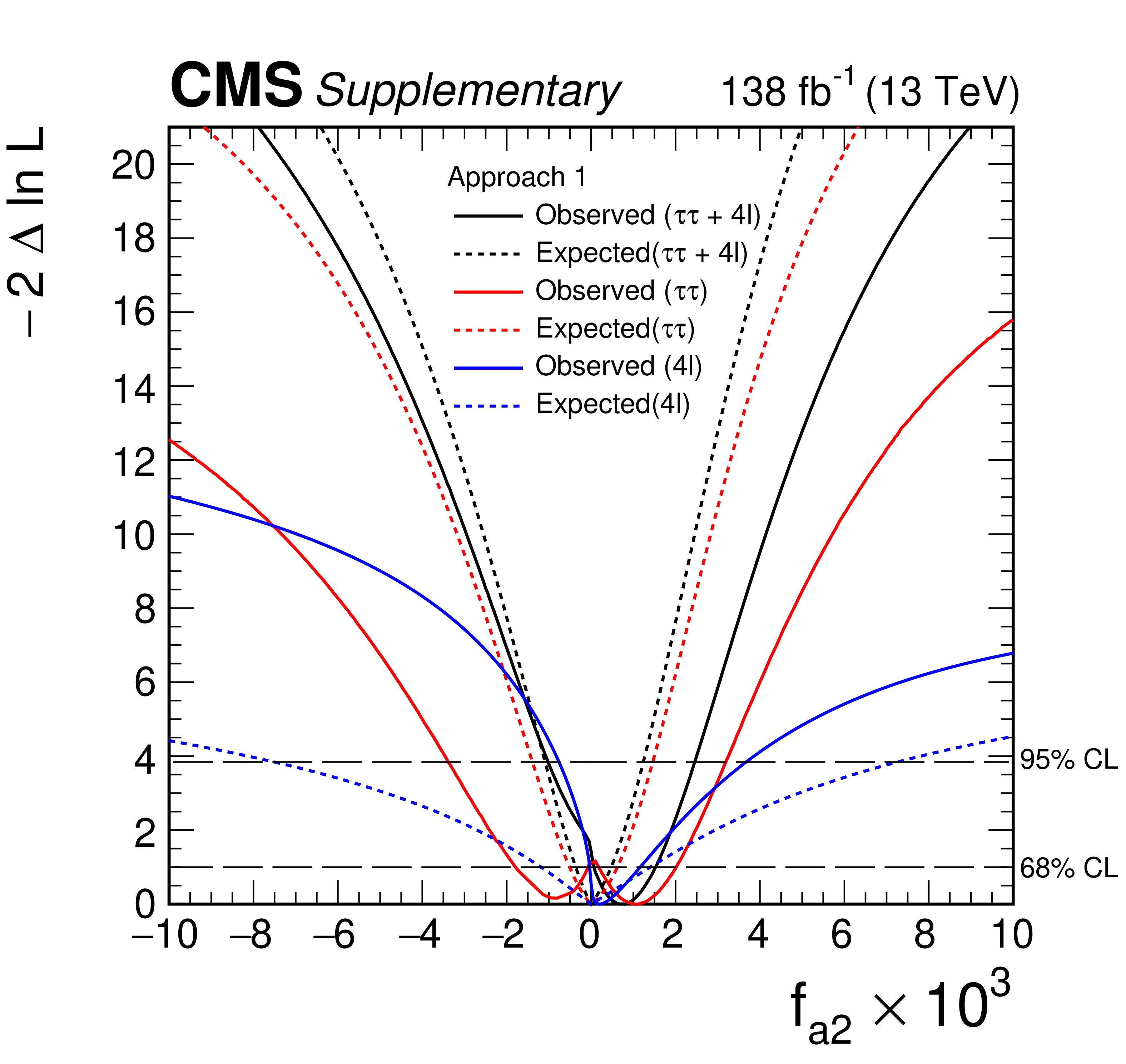
Observed (solid) and expected (dashed) likelihood scans of ${f_{a3}} $ (upper left), ${f_{a2}} $ (upper right), ${f_{\Lambda 1}} $ (lower left), and ${f_{\Lambda 1}^{\mathrm{Z} \gamma}}$ (lower right) in Approach 1 (${a_i^{\mathrm{W} \mathrm{W}}=a_i^{\mathrm{Z} \mathrm{Z}}}$). |
png pdf |
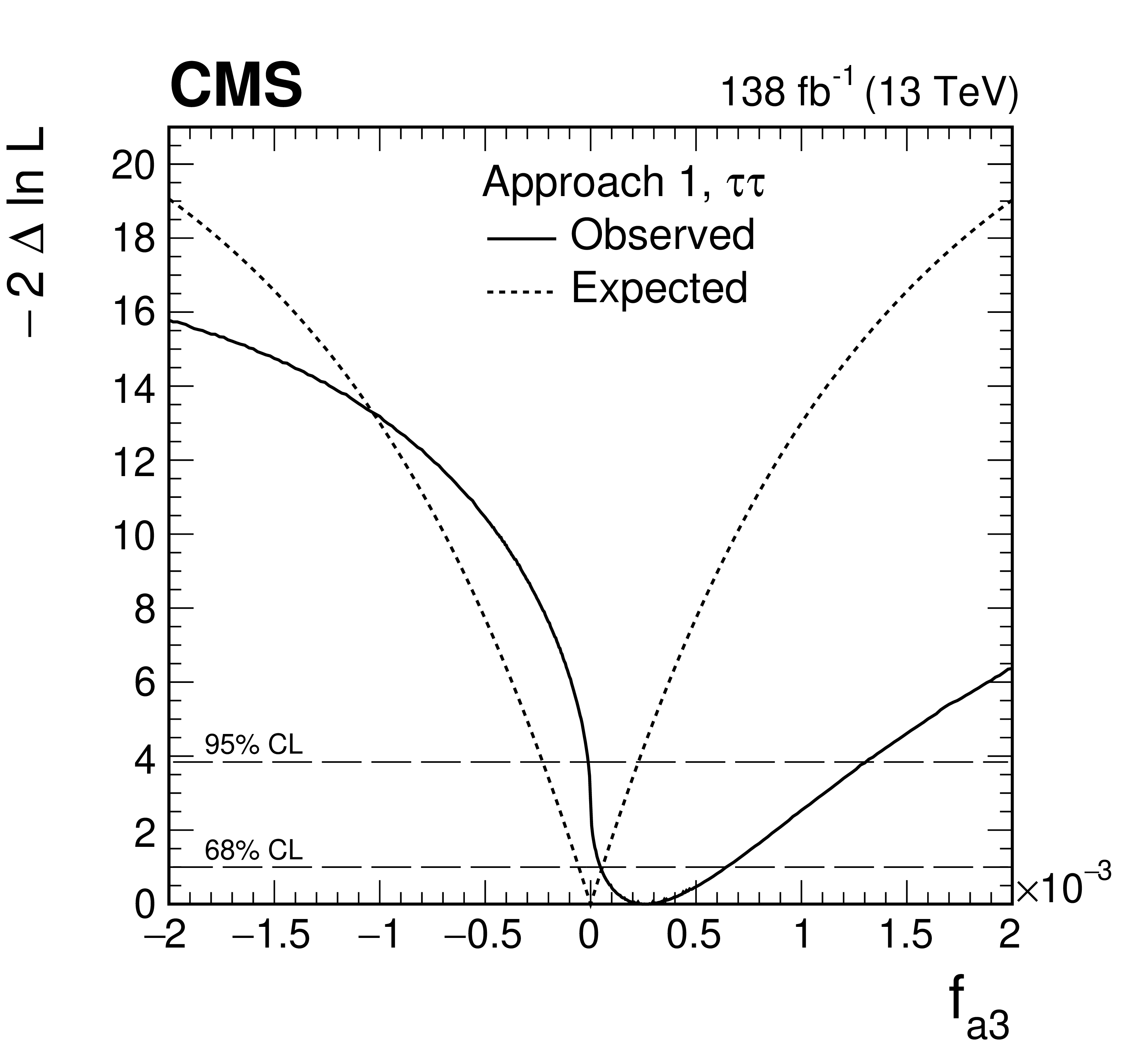
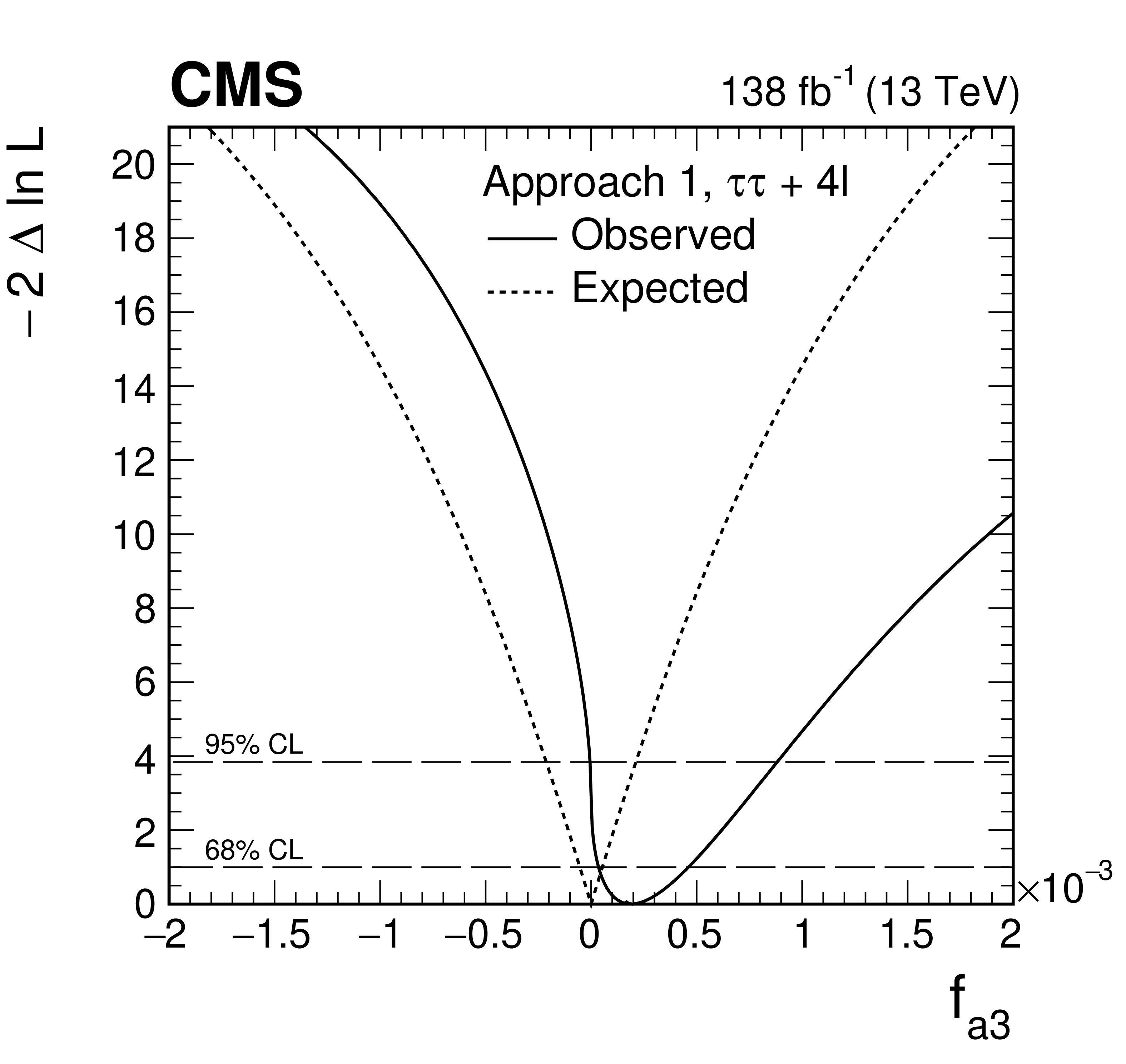
Figure 9-a:
Observed (solid) and expected (dashed) likelihood scans of ${f_{a3}} in Approach 1 (${a_i^{\mathrm{W} \mathrm{W}}=a_i^{\mathrm{Z} \mathrm{Z}}}$). |

png pdf |
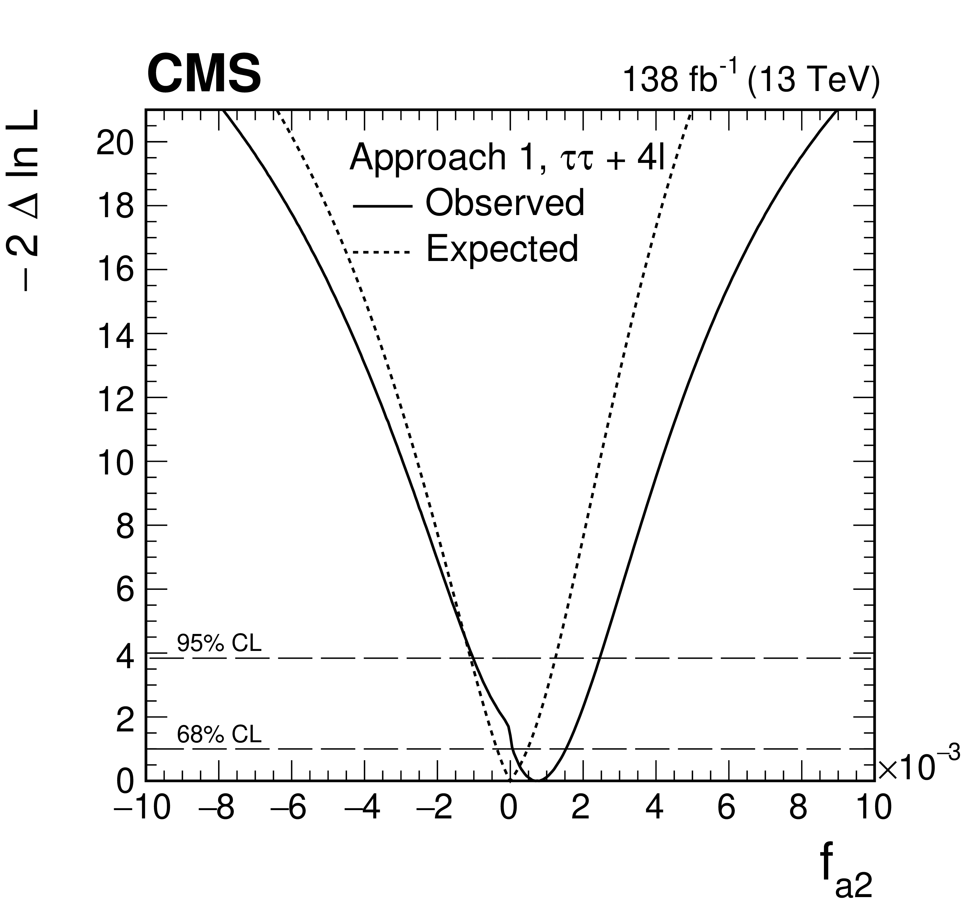
Figure 9-b:
Observed (solid) and expected (dashed) likelihood scans of ${f_{a2}} $ in Approach 1 (${a_i^{\mathrm{W} \mathrm{W}}=a_i^{\mathrm{Z} \mathrm{Z}}}$). |
png pdf |
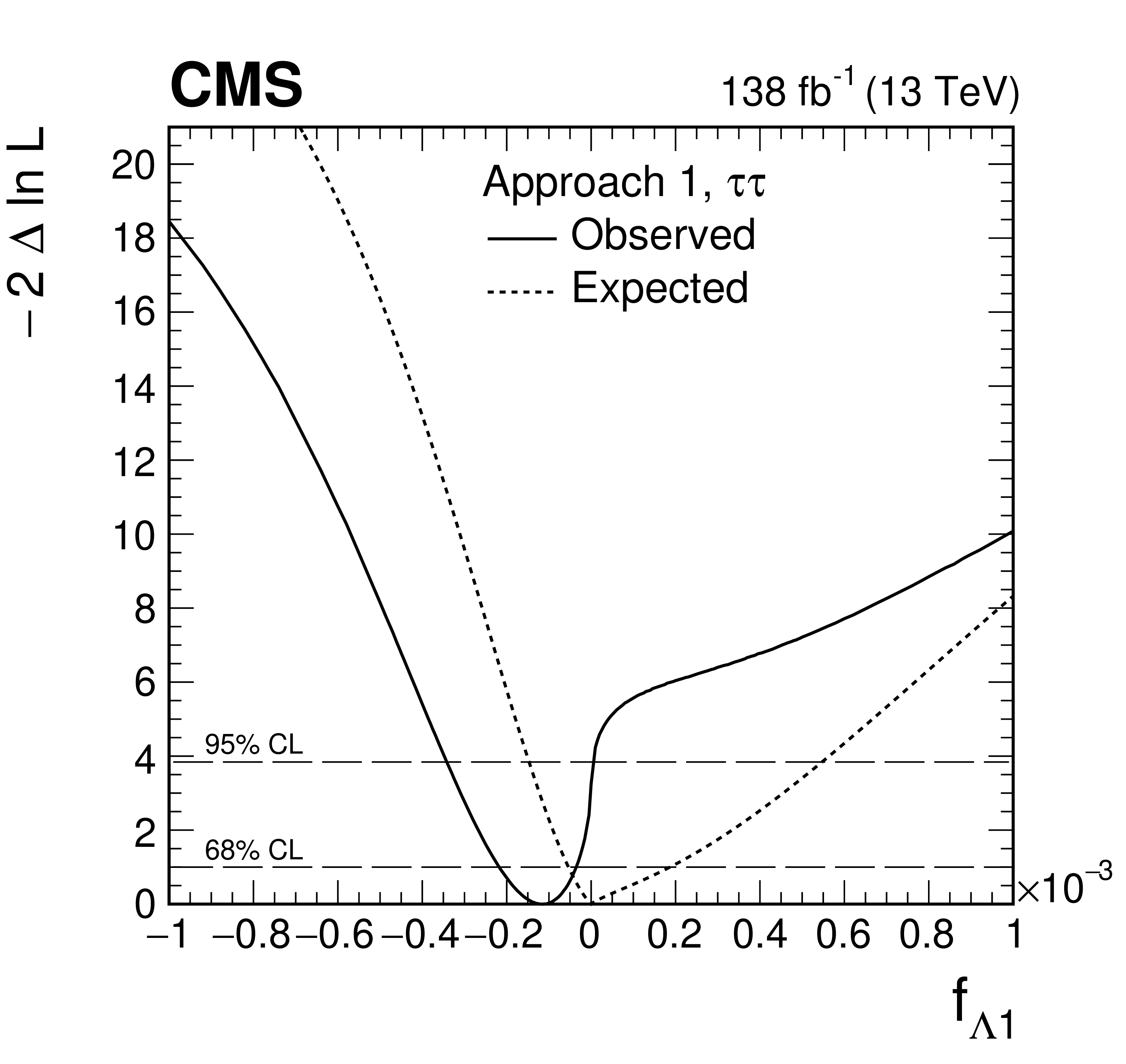
Figure 9-c:
Observed (solid) and expected (dashed) likelihood scans of ${f_{\Lambda 1}} $ in Approach 1 (${a_i^{\mathrm{W} \mathrm{W}}=a_i^{\mathrm{Z} \mathrm{Z}}}$). |

png pdf |
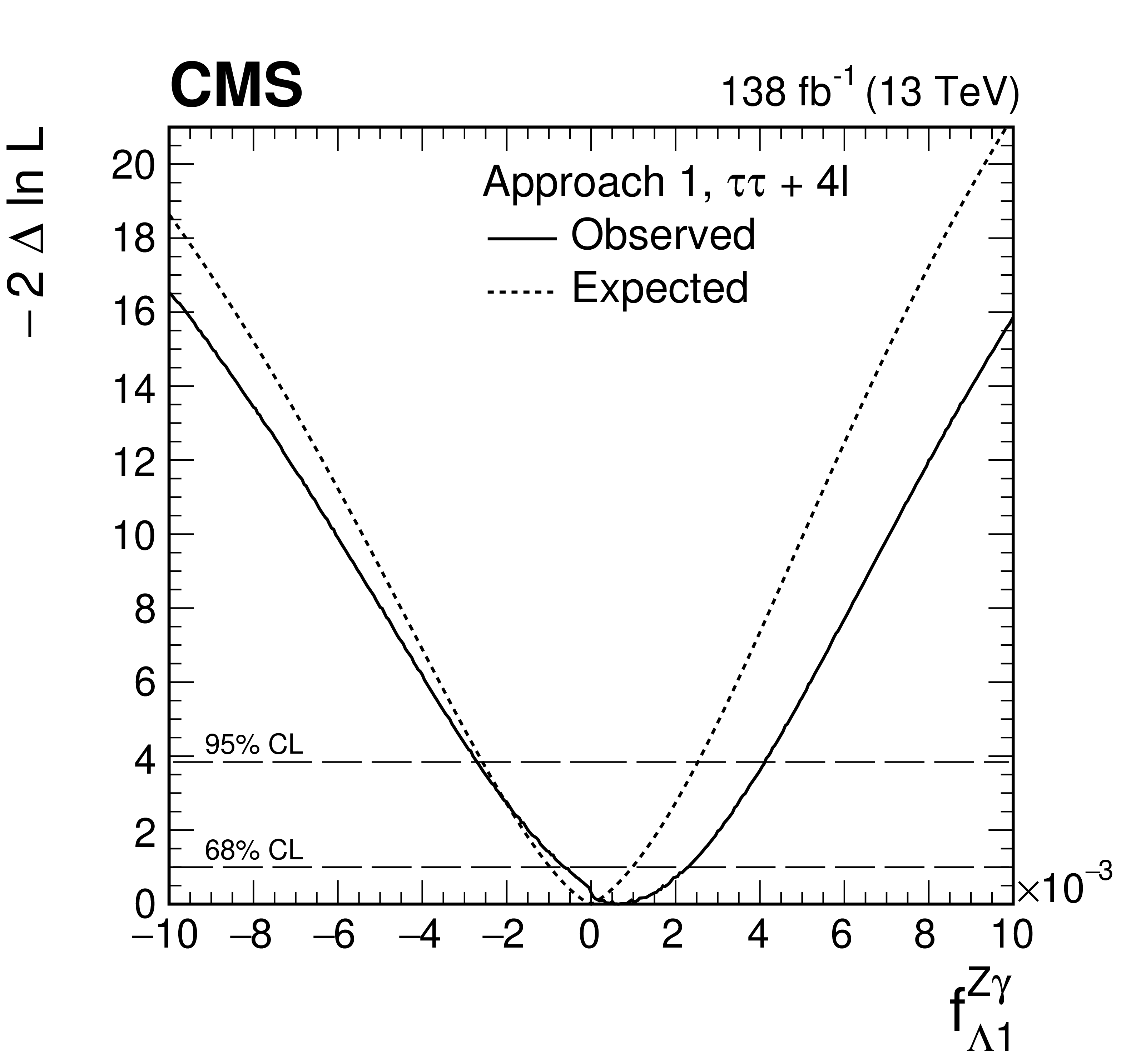
Figure 9-d:
Observed (solid) and expected (dashed) likelihood scans of ${f_{\Lambda 1}^{\mathrm{Z} \gamma}}$ in Approach 1 (${a_i^{\mathrm{W} \mathrm{W}}=a_i^{\mathrm{Z} \mathrm{Z}}}$). |

png pdf |
Figure 10:
Observed (solid) and expected (dashed) likelihood scans of ${f_{a3}} $ in Approach 2. |
png pdf |
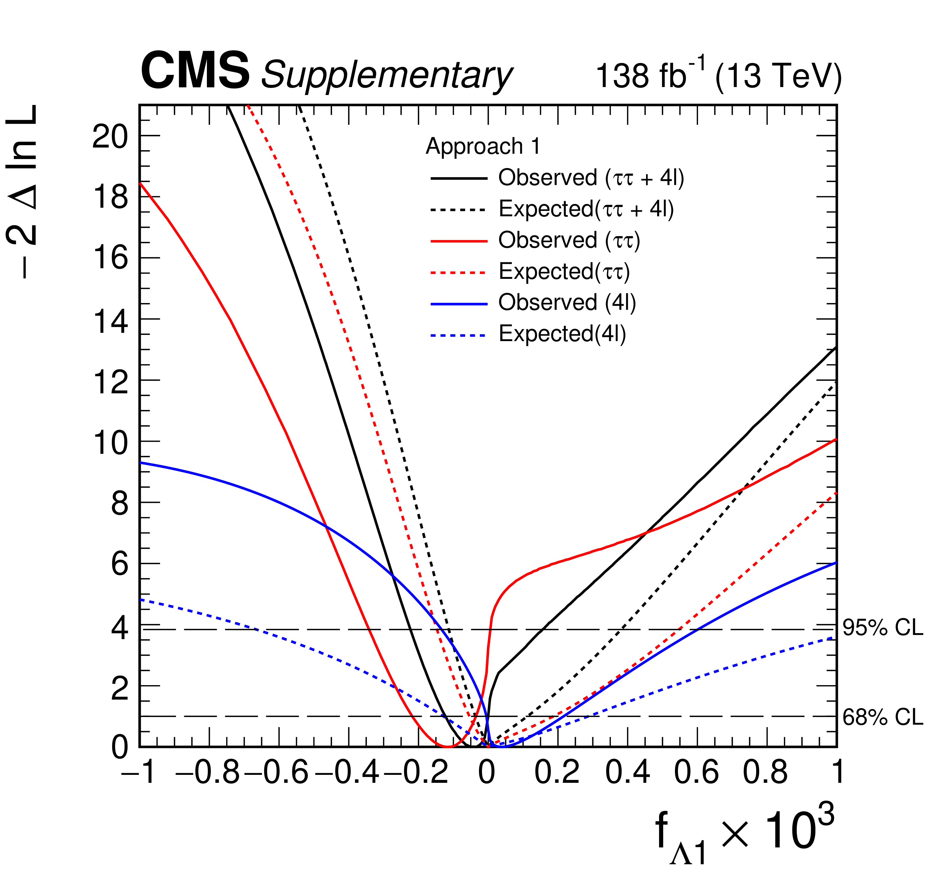
Figure 11:
Observed (solid) and expected (dashed) likelihood scans of ${f_{a3}} $ (upper left), ${f_{a2}} $ (upper right), ${f_{\Lambda 1}} $ (lower left), and ${f_{\Lambda 1}^{\mathrm{Z} \gamma}}$ (lower right) in Approach 1 ($a_i^{\mathrm{W} \mathrm{W}}$ = $a_i^{\mathrm{Z} \mathrm{Z}}$) obtained with the combination of results using the ${\mathrm{H} \to \tau \tau}$ and ${\mathrm{H} \to 4\ell}$ [21] decay channels. |
png pdf |
Figure 11-a:
Observed (solid) and expected (dashed) likelihood scans of ${f_{a3}} $ in Approach 1 ($a_i^{\mathrm{W} \mathrm{W}}$ = $a_i^{\mathrm{Z} \mathrm{Z}}$) obtained with the combination of results using the ${\mathrm{H} \to \tau \tau}$ and ${\mathrm{H} \to 4\ell}$ [21] decay channels. |
png pdf |
Figure 11-b:
Observed (solid) and expected (dashed) likelihood scans of ${f_{a2}} $ in Approach 1 ($a_i^{\mathrm{W} \mathrm{W}}$ = $a_i^{\mathrm{Z} \mathrm{Z}}$) obtained with the combination of results using the ${\mathrm{H} \to \tau \tau}$ and ${\mathrm{H} \to 4\ell}$ [21] decay channels. |

png pdf |
Figure 11-c:
Observed (solid) and expected (dashed) likelihood scans of ${f_{\Lambda 1}} $ in Approach 1 ($a_i^{\mathrm{W} \mathrm{W}}$ = $a_i^{\mathrm{Z} \mathrm{Z}}$) obtained with the combination of results using the ${\mathrm{H} \to \tau \tau}$ and ${\mathrm{H} \to 4\ell}$ [21] decay channels. |
png pdf |
Figure 11-d:
Observed (solid) and expected (dashed) likelihood scans of ${f_{\Lambda 1}^{\mathrm{Z} \gamma}}$ in Approach 1 ($a_i^{\mathrm{W} \mathrm{W}}$ = $a_i^{\mathrm{Z} \mathrm{Z}}$) obtained with the combination of results using the ${\mathrm{H} \to \tau \tau}$ and ${\mathrm{H} \to 4\ell}$ [21] decay channels. |

png pdf |
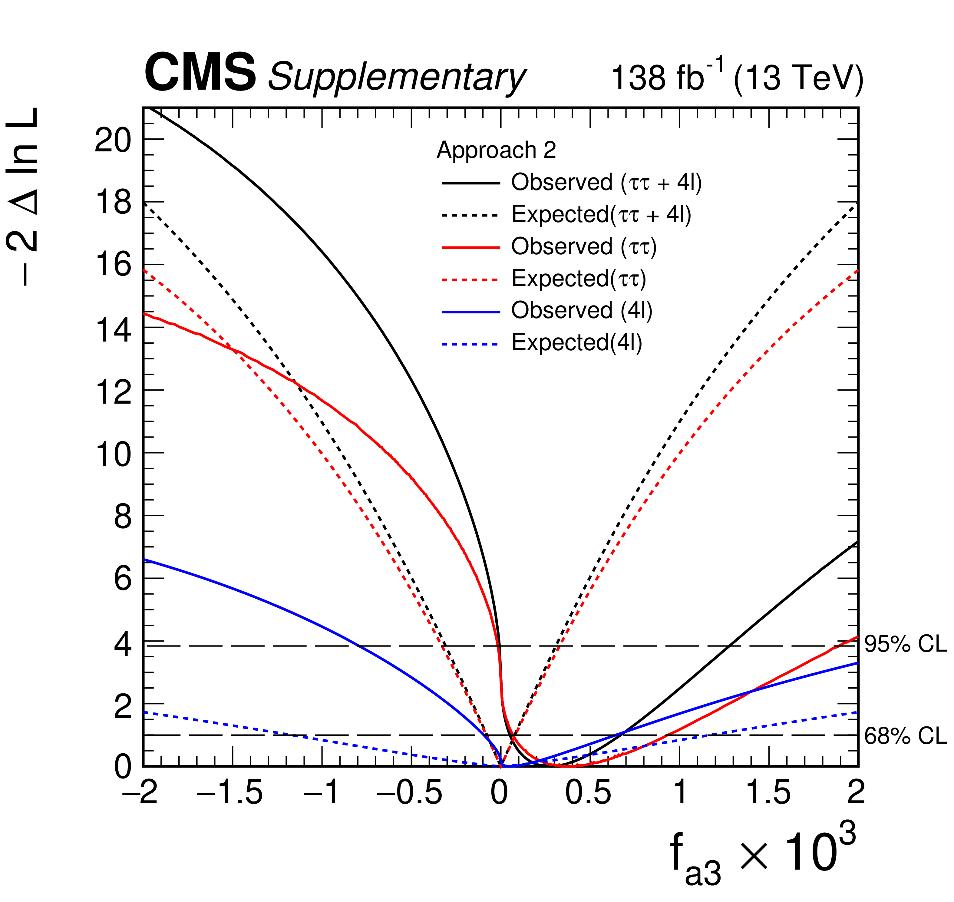
Figure 12:
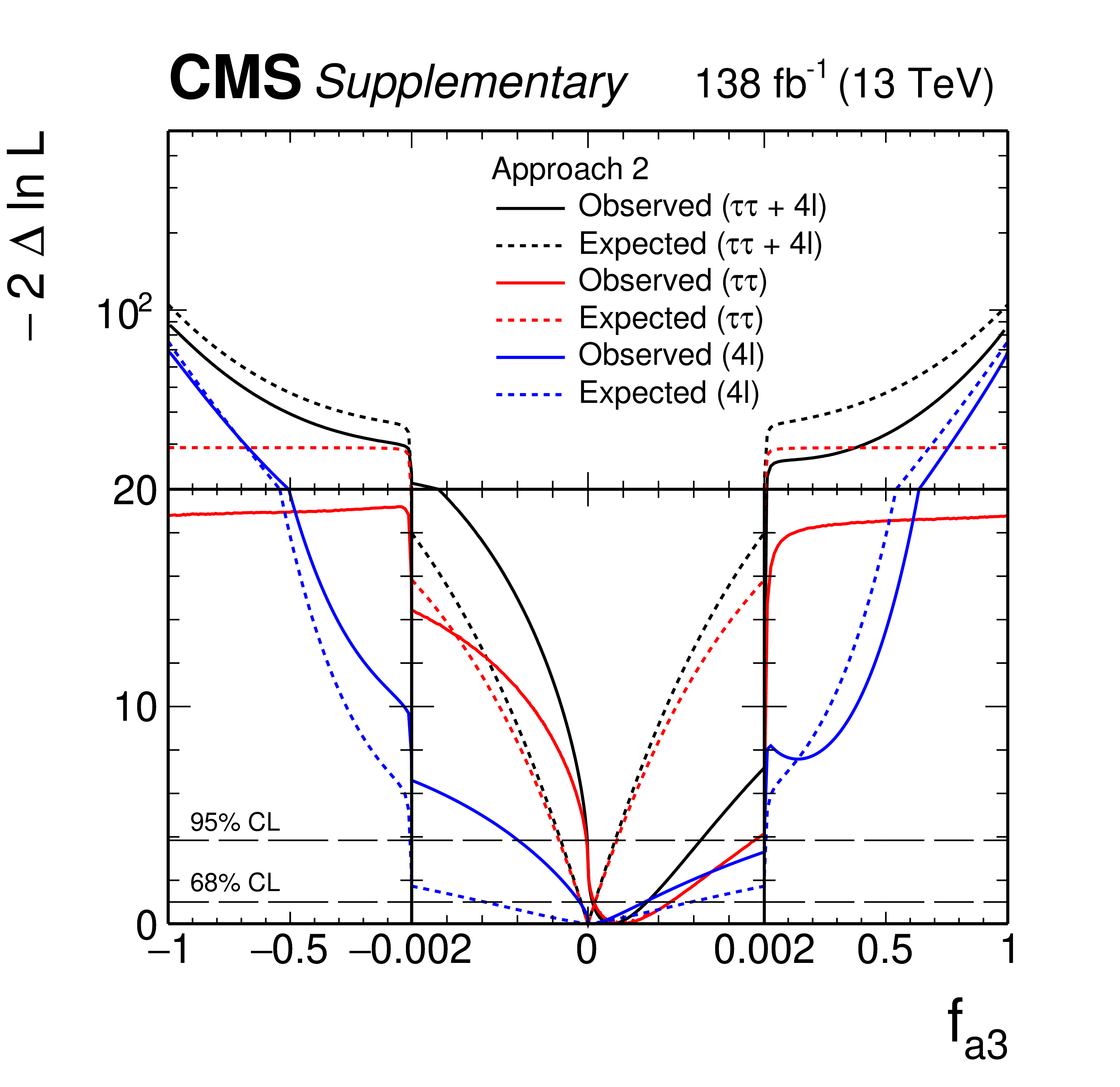
Observed (solid) and expected (dashed) likelihood scans of ${f_{a3}} $ in Approach 2 (defined in Section 2) obtained with the combination of results using the ${\mathrm{H} \to \tau \tau}$ and ${\mathrm{H} \to 4\ell}$ [21] decay channels. |
png pdf |
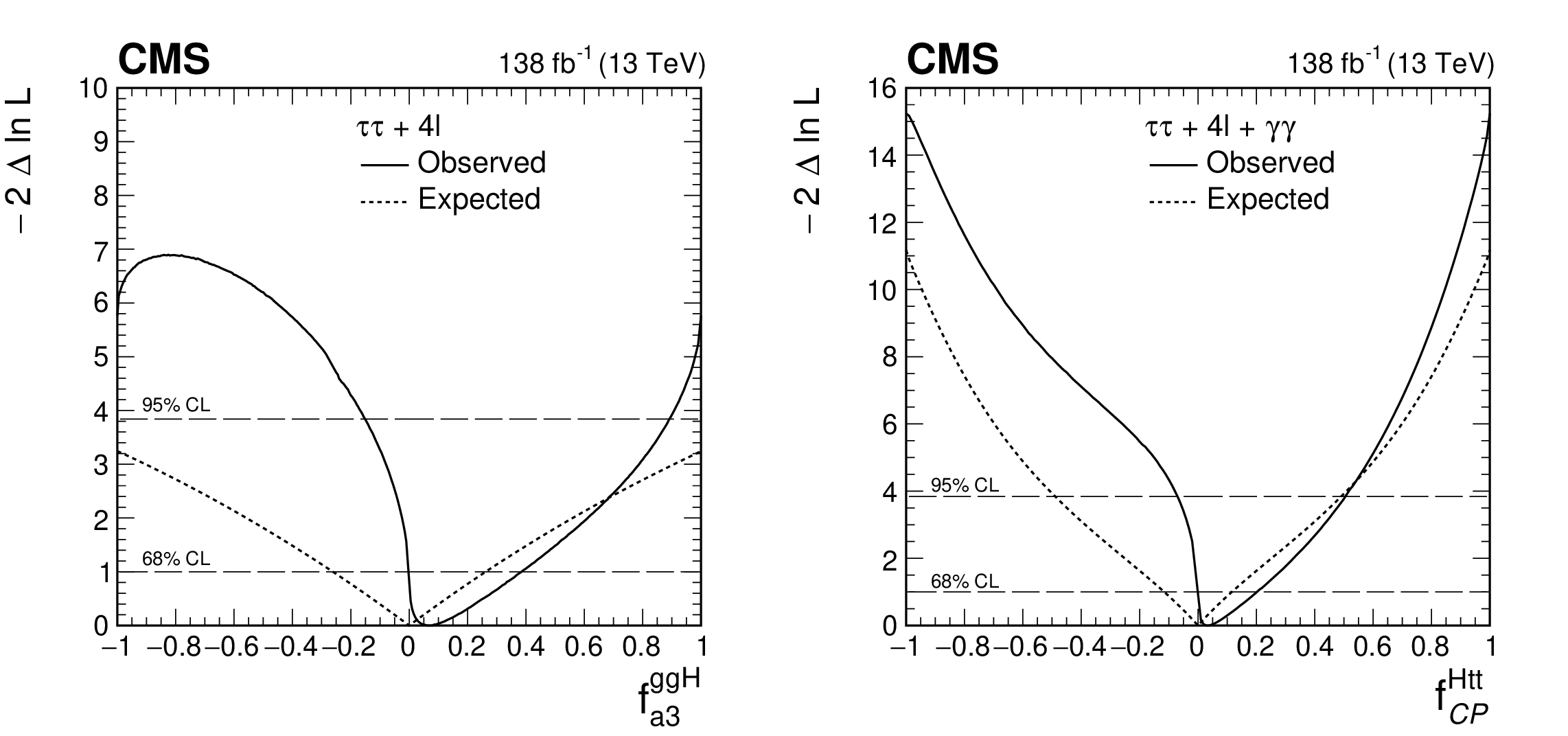
Figure 13:
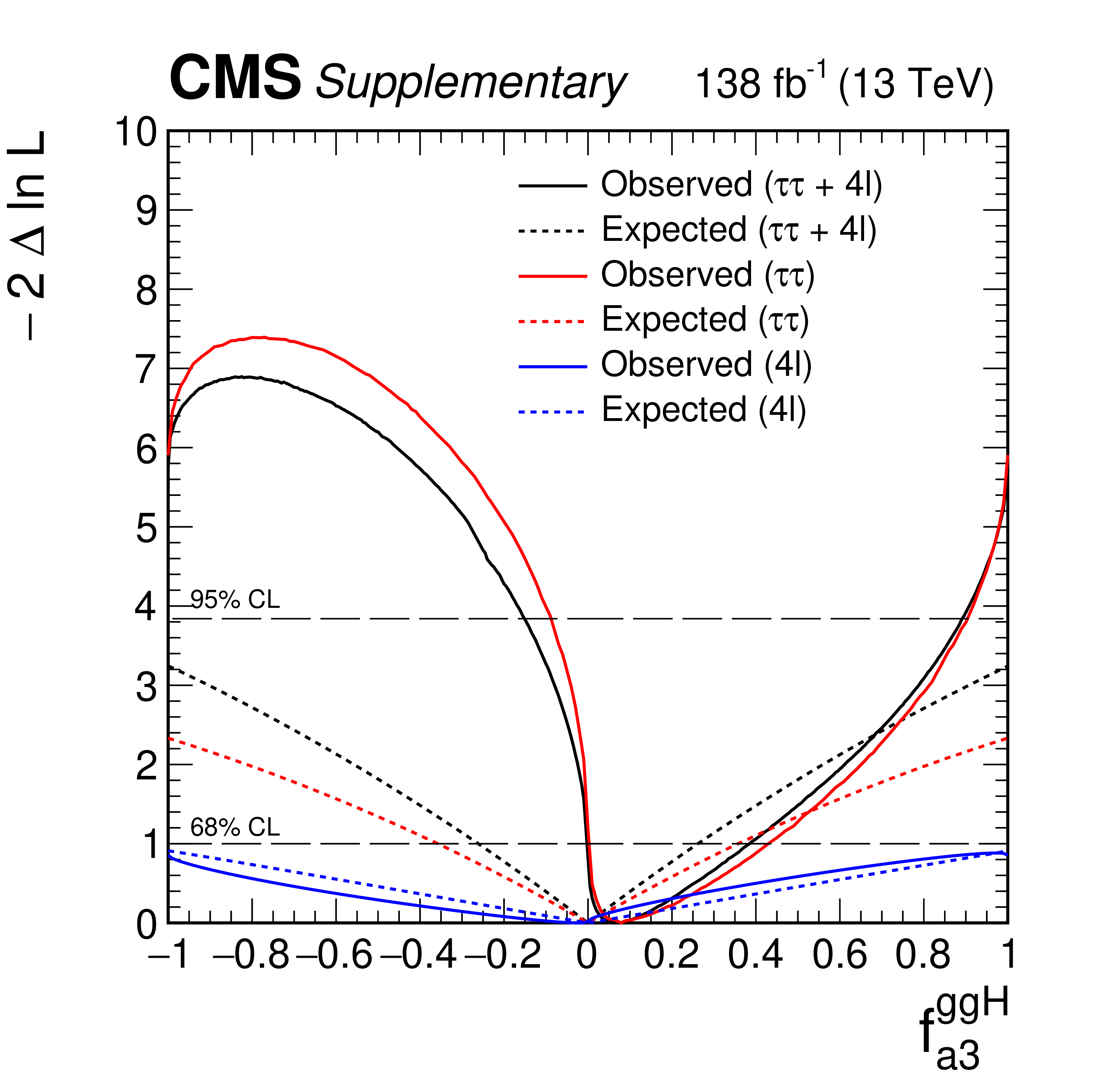
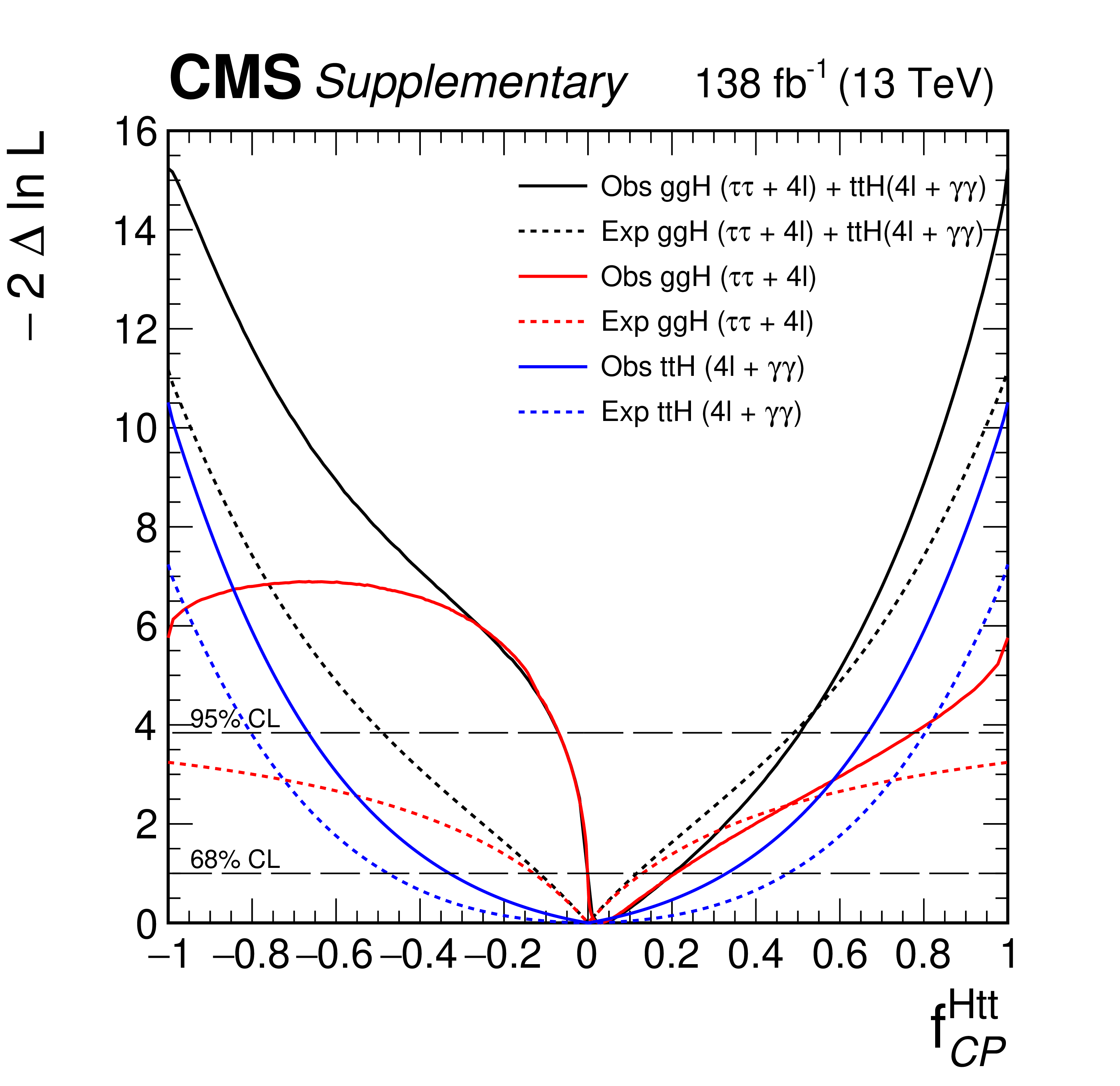
Left: the observed (solid) and expected (dashed) likelihood scans of ${f_{a3}^{\mathrm{g} \mathrm{g} \mathrm{H}}}$ obtained with the combination of results using the ${\mathrm{H} \to \tau \tau}$ and ${\mathrm{H} \to 4\ell}$ [21] decay channels. Right: The observed (solid) and expected (dashed) likelihood scans of ${f_{\text{CP}}^{\mathrm{H} \mathrm{t} \mathrm{t}}}$ obtained with the combination of results using the ${\mathrm{H} \to \tau \tau}$, ${\mathrm{H} \to 4\ell}$ [21], and ${\mathrm{H} \to \gamma \gamma}$ [20] decay channels. |

png pdf |
Figure 13-a:
The observed (solid) and expected (dashed) likelihood scans of ${f_{a3}^{\mathrm{g} \mathrm{g} \mathrm{H}}}$ obtained with the combination of results using the ${\mathrm{H} \to \tau \tau}$ and ${\mathrm{H} \to 4\ell}$ [21] decay channels. |
png pdf |
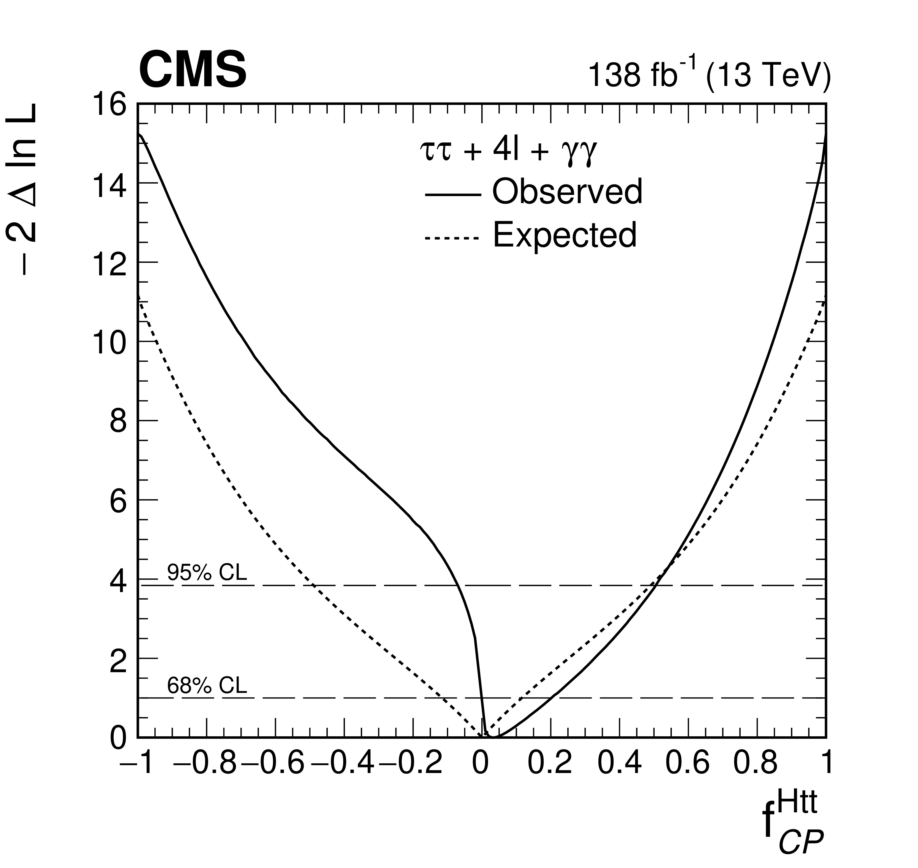
Figure 13-b:
The observed (solid) and expected (dashed) likelihood scans of ${f_{\text{CP}}^{\mathrm{H} \mathrm{t} \mathrm{t}}}$ obtained with the combination of results using the ${\mathrm{H} \to \tau \tau}$, ${\mathrm{H} \to 4\ell}$ [21], and ${\mathrm{H} \to \gamma \gamma}$ [20] decay channels. |

png pdf |
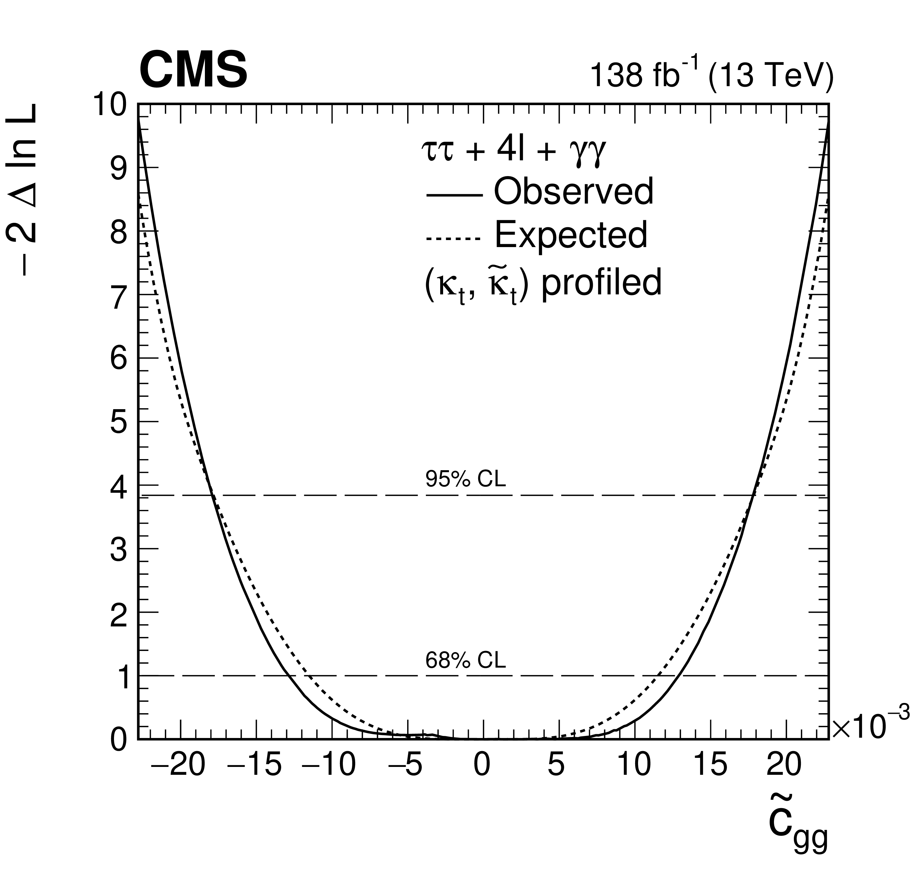
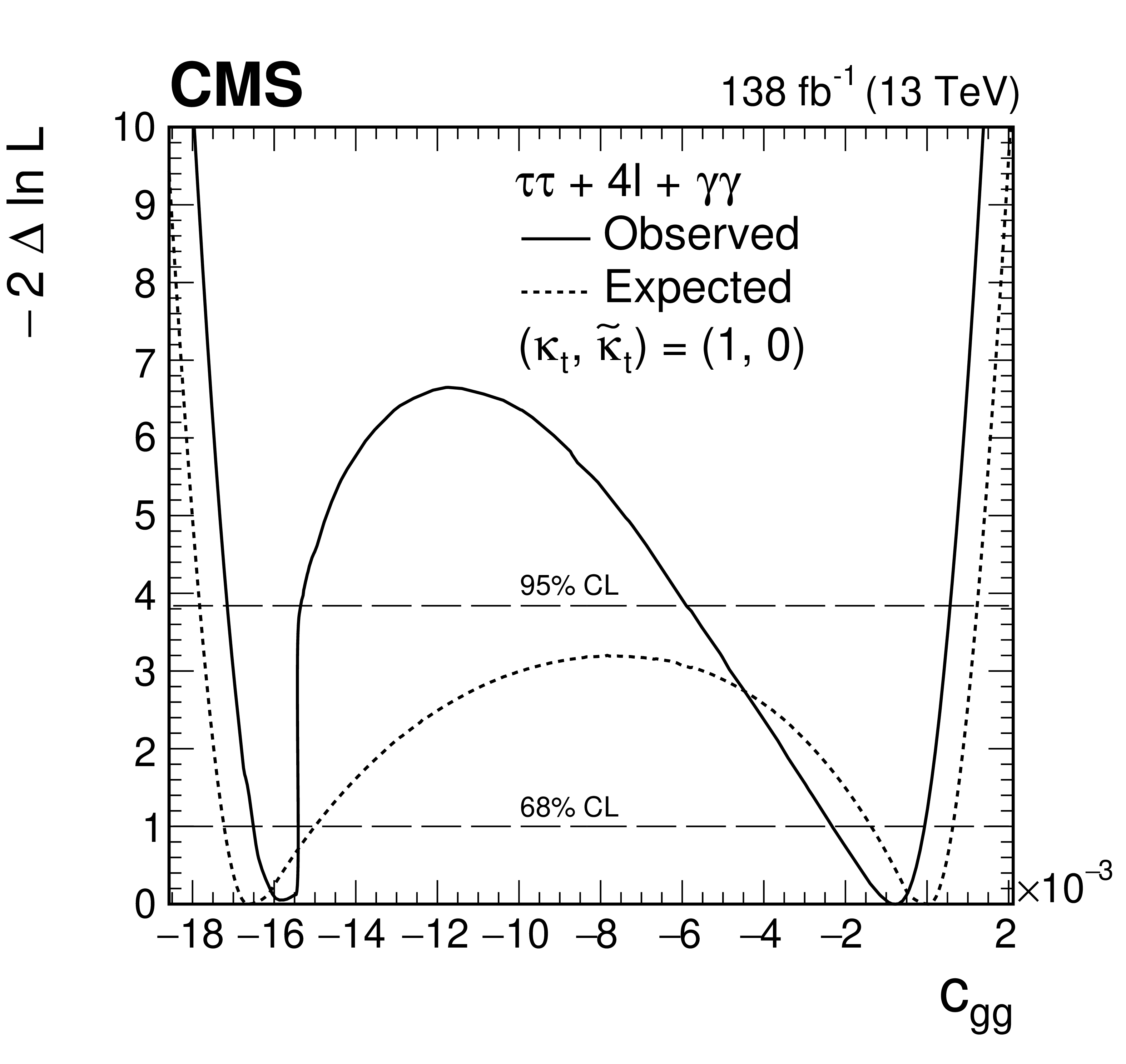
Figure 14:
Observed (solid) and expected (dashed) likelihood scans of ${c_{\mathrm{g} \mathrm{g}}}$ (left) and ${\tilde{c}_{\mathrm{g} \mathrm{g}}}$ (right) with ${\kappa _\mathrm {t}}$ and ${\tilde{\kappa}}_\mathrm {t}$ profiled (upper) and fixed to SM expectation (lower) using the ${\mathrm{H} \to \tau \tau}$, ${\mathrm{H} \to 4\ell}$ [21], and ${\mathrm{H} \to \gamma \gamma}$ [20] decay channels. |

png pdf |
Figure 14-a:
Observed (solid) and expected (dashed) likelihood scans of ${c_{\mathrm{g} \mathrm{g}}}$ with ${\kappa _\mathrm {t}}$ and ${\tilde{\kappa}}_\mathrm {t}$ profiled using the ${\mathrm{H} \to \tau \tau}$, ${\mathrm{H} \to 4\ell}$ [21], and ${\mathrm{H} \to \gamma \gamma}$ [20] decay channels. |
png pdf |
Figure 14-b:
Observed (solid) and expected (dashed) likelihood scans of ${\tilde{c}_{\mathrm{g} \mathrm{g}}}$ with ${\kappa _\mathrm {t}}$ and ${\tilde{\kappa}}_\mathrm {t}$ fixed to SM expectation using the ${\mathrm{H} \to \tau \tau}$, ${\mathrm{H} \to 4\ell}$ [21], and ${\mathrm{H} \to \gamma \gamma}$ [20] decay channels. |
png pdf |
Figure 14-c:
Observed (solid) and expected (dashed) likelihood scans of ${c_{\mathrm{g} \mathrm{g}}}$ with ${\kappa _\mathrm {t}}$ and ${\tilde{\kappa}}_\mathrm {t}$ profiled using the ${\mathrm{H} \to \tau \tau}$, ${\mathrm{H} \to 4\ell}$ [21], and ${\mathrm{H} \to \gamma \gamma}$ [20] decay channels. |

png pdf |
Figure 14-d:
Observed (solid) and expected (dashed) likelihood scans of ${\tilde{c}_{\mathrm{g} \mathrm{g}}}$ with ${\kappa _\mathrm {t}}$ and ${\tilde{\kappa}}_\mathrm {t}$ fixed to SM expectation using the ${\mathrm{H} \to \tau \tau}$, ${\mathrm{H} \to 4\ell}$ [21], and ${\mathrm{H} \to \gamma \gamma}$ [20] decay channels. |
| Tables | |
png pdf |
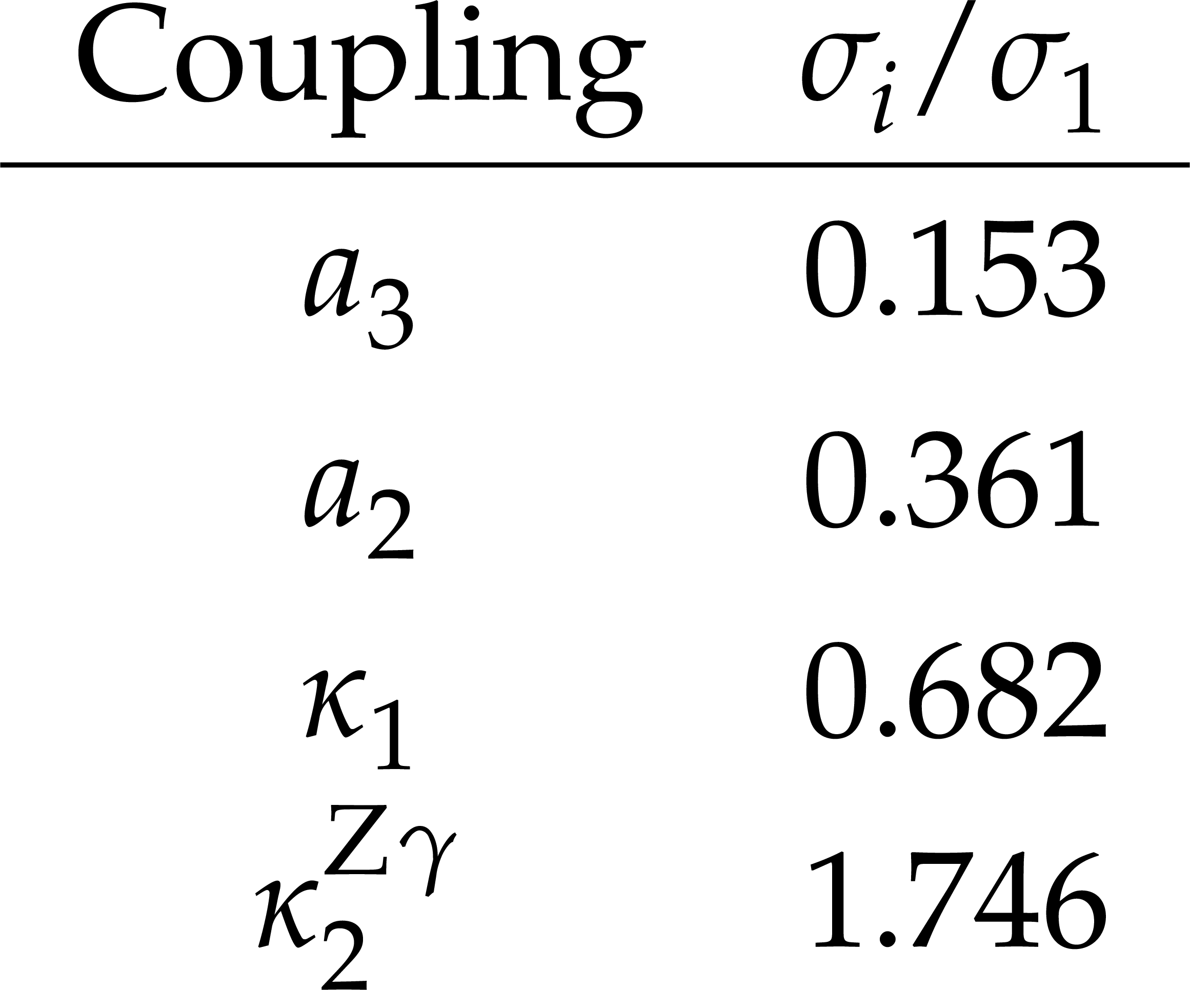
Table 1:
Cross sections for the anomalous contributions ($\sigma _i$) used to define the fractional cross sections [21]. The $\sigma _i$ values are defined as the cross section computed with $a_{i}=$ 1 and all other couplings set to zero. All cross sections are given relative to the SM value ($\sigma _1$). In the case of the $\kappa _{1}$ and $\kappa _{2}^{\mathrm{Z} \gamma}$ couplings, the numerical values $\Lambda _1 = \Lambda _1^{\mathrm{Z} \gamma} = $ 100 GeV are considered so as to keep all coefficients of similar order of magnitude. |

png pdf |
Table 2:
List of discriminants for separating anomalous couplings from the SM contribution. |
png pdf |
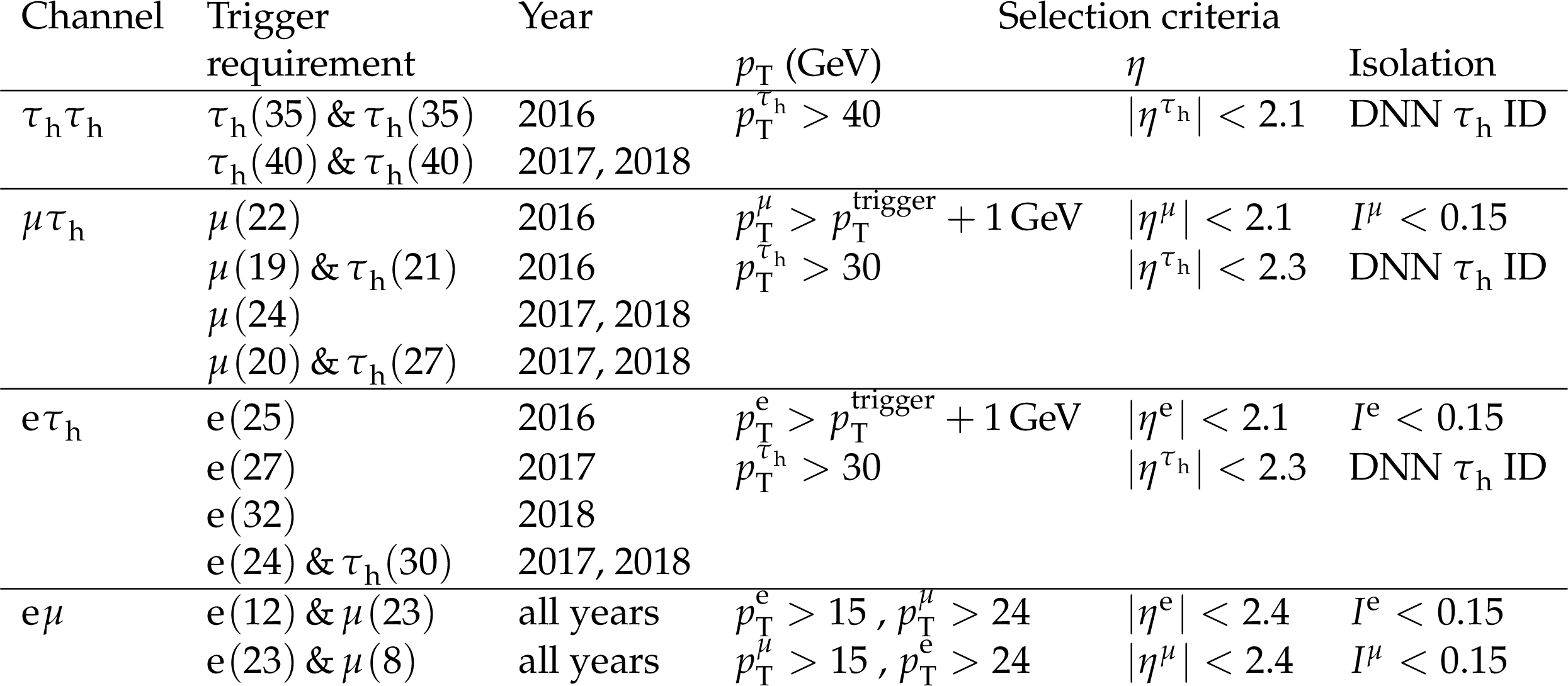
Table 3:
Kinematic selection requirements for the four di-$\tau $ decay channels. The trigger requirement is defined by a combination of trigger candidates with ${p_{\mathrm {T}}}$ over a given threshold, indicated inside parentheses in GeV. The pseudorapidity thresholds come from trigger and object reconstruction constraints. The $ {p_{\mathrm {T}}} $ thresholds for the lepton selection are driven by the trigger requirements, except for the $ {\tau _\mathrm {h}} $ candidate in the $\mu {\tau _\mathrm {h}} $ and e$ {\tau _\mathrm {h}} $ channels, and the sub-leading lepton in the e$ \mu $ channel, where they have been optimized to increase the analysis sensitivity. |

png pdf |
Table 4:
Sources of systematic uncertainties. |
png pdf |
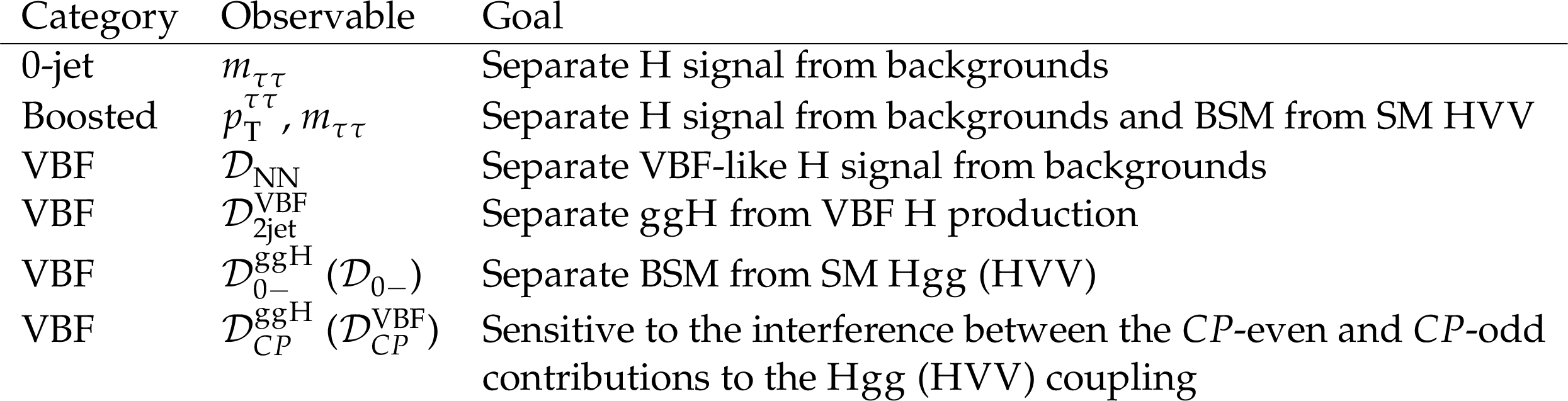
Table 5:
List of observables used in the MELA method. |
png pdf |
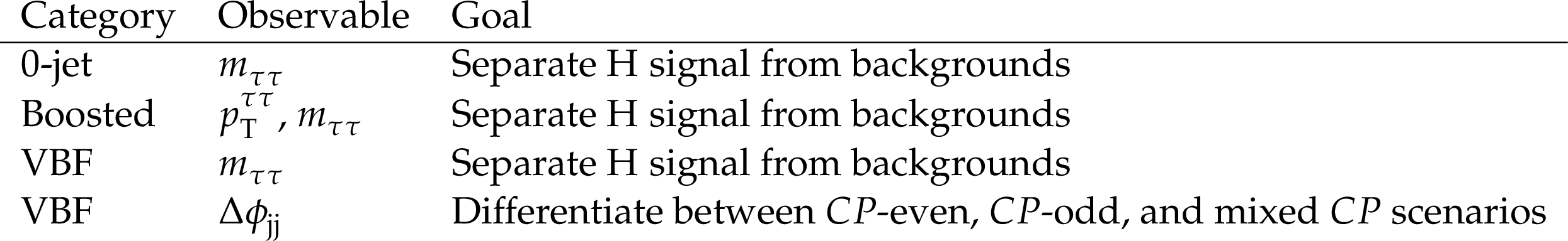
Table 6:
List of observables used in the ${\Delta \phi _{\mathrm {jj}}}$ method. |
png pdf |
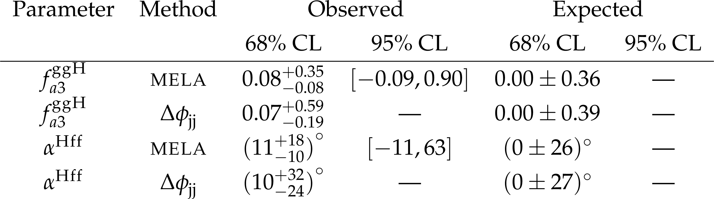
Table 7:
Allowed 68% (central values with uncertainties) and 95% CL (in square brackets) intervals on anomalous Hgg coupling parameters using the ${\mathrm{H} \to \tau \tau}$ decay. The use of "-" indicates cases where no exclusion at the 95% CL was found. As indicated in the Table, the results are presented for the MELA method, as well as the ${\Delta \phi _{\mathrm {jj}}}$ method for comparison. The final results of this study are from the MELA method. The ${\alpha ^{\mathrm{H} \mathrm {ff}}}$ results are derived from ${f_{a3}^{\mathrm{g} \mathrm{g} \mathrm{H}}}$ following Eqs. (5), (6), and (10). |
png pdf |
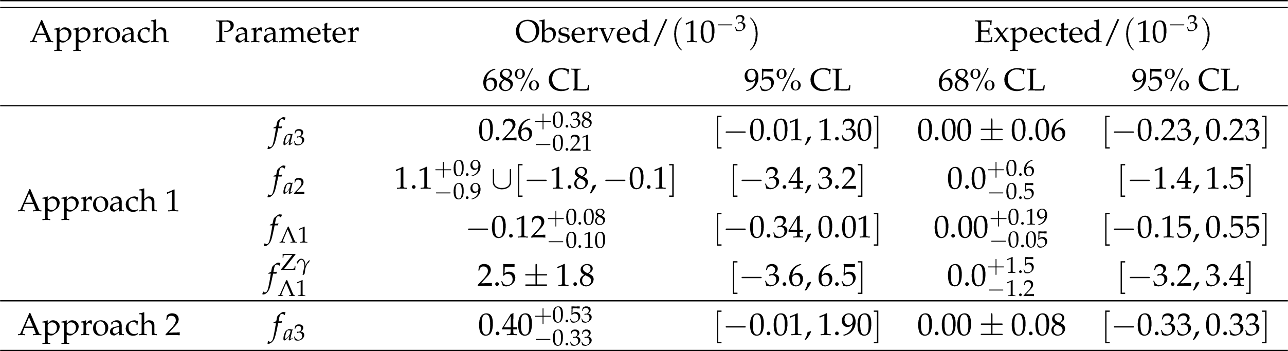
Table 8:
Allowed 68% (central values with uncertainties) and 95% CL (in square brackets) intervals on anomalous HVV coupling parameters using the ${\mathrm{H} \to \tau \tau}$ decay. Approaches 1 and 2 refer to the choice of the relationship between the $a_i^{\mathrm{W} \mathrm{W}}$ and $a_i^{\mathrm{Z} \mathrm{Z}}$ couplings, defined in Section 2. For the observed ${f_{a2}} $scan, there is a second region allowed at the 68% CL away from the best fit value. We use the union symbol ($\cup $) to display the additional allowed ${f_{a2}} $range in this case. |

png pdf |
Table 9:
Allowed 68% (central values with uncertainties) and 95% CL (in square brackets) intervals on anomalous HVV coupling parameters using the ${\mathrm{H} \to \tau \tau}$ and ${\mathrm{H} \to 4\ell}$ [21] decay channels, using two approaches described in Section 2 that define the relationship between the $a_i^{\mathrm{W} \mathrm{W}}$ and $a_i^{\mathrm{Z} \mathrm{Z}}$ couplings. |
png pdf |
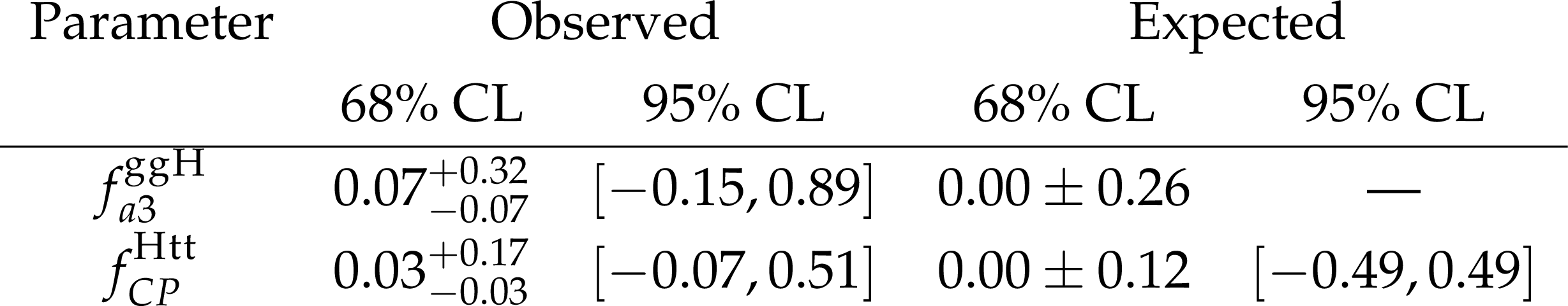
Table 10:
Allowed 68% (central values with uncertainties) and 95% CL (in square brackets) intervals on ${f_{a3}^{\mathrm{g} \mathrm{g} \mathrm{H}}}$, from the combination of the ${\mathrm{H} \to \tau \tau}$ and ${\mathrm{H} \to 4\ell}$ [21] decay channels, and ${f_{\text{CP}}^{\mathrm{H} \mathrm{t} \mathrm{t}}}$, from the combination of the ${\mathrm{H} \to \tau \tau}$, ${\mathrm{H} \to 4\ell}$ [21], and ${\mathrm{H} \to \gamma \gamma}$ [20] decay channels. |
png pdf |
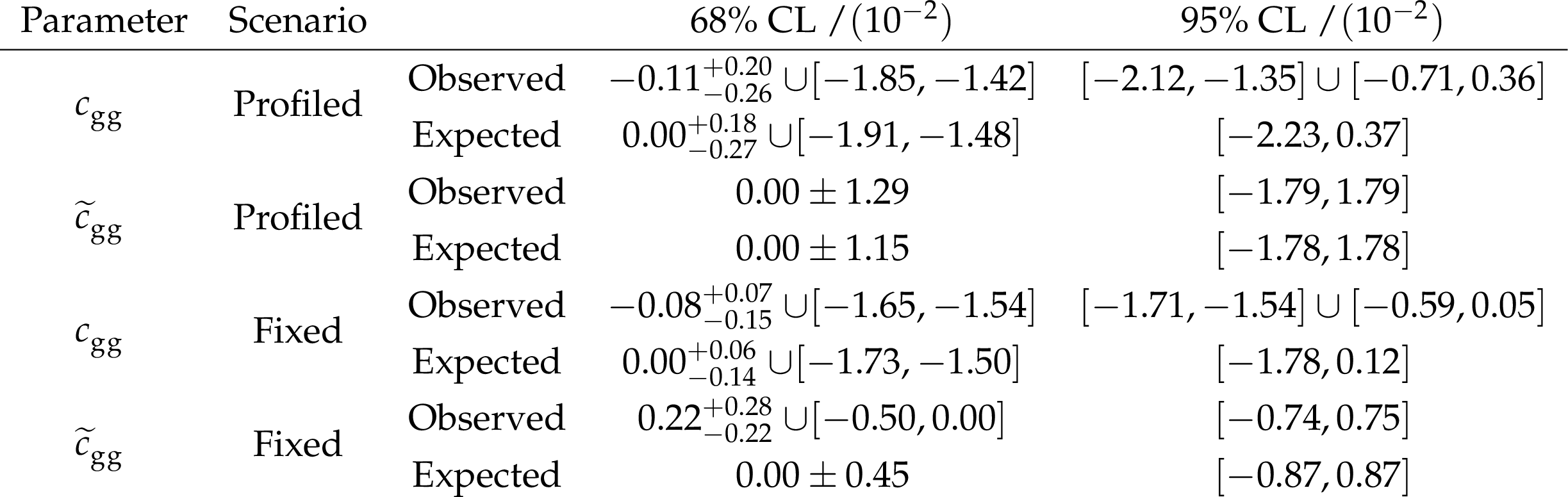
Table 11:
Allowed 68% (central values with uncertainties) and 95% CL (in square brackets) intervals on ${c_{\mathrm{g} \mathrm{g}}}$ and ${\tilde{c}_{\mathrm{g} \mathrm{g}}}$ using the ${\mathrm{H} \to \tau \tau}$, ${\mathrm{H} \to 4\ell}$ [21], and ${\mathrm{H} \to \gamma \gamma}$ [20] decay channels. Results are presented for two scenarios: ${\kappa _\mathrm {t}}$ and ${\tilde{\kappa}}_\mathrm {t}$ profiled in the fit, and ${\kappa _\mathrm {t}}$ and ${\tilde{\kappa}}_\mathrm {t}$ fixed to the SM expectation. In instances where there is a second allowed region away from the best fit value at a given CL, we use the union symbol ($\cup $) to display the additional allowed ${\tilde{c}_{\mathrm{g} \mathrm{g}}} / {c_{\mathrm{g} \mathrm{g}}}$ range. |
| Summary |
| A study is presented of anomalous interactions of the Higgs boson (H) with vector bosons, including violation, using its associated production with two hadronic jets in gluon fusion (ggH), vector boson fusion (VBF), and associated production with a vector boson, and a subsequent decay to a pair of $\tau$ leptons. Constraints have been set on the CP-violating effects in ggH production in terms of the effective cross section ratio ${f_{a3}^{\mathrm{g}\mathrm{g}\mathrm{H}}} $, or equivalently the effective mixing angle ${\alpha^{\mathrm{H}\mathrm{ff}}} $, using matrix element techniques. The ggH production analysis results in the most stringent limits on violation in ggH production to date. In the VBF production analysis, constraints on the CP-violating parameter ${f_{a3}} $ and on the CP-conserving parameters ${f_{a2}} $, ${f_{\Lambda 1}} $, and ${f_{\Lambda 1}^{\mathrm{Z}\gamma}}$ have been set using matrix element techniques. Further constraints were obtained in the combination of the $\mathrm{H} \to \tau \tau$, $\mathrm{H} \to 4\ell$, and $\mathrm{H} \to \gamma\gamma$ channels. The combination improves the limits on the anomalous coupling parameters typically by about 20-50%. The analysis excludes the pure CP-odd scenario of the Higgs coupling to gluons with a significance of 2.4 standard deviations. |
| Additional Figures | |
png pdf |
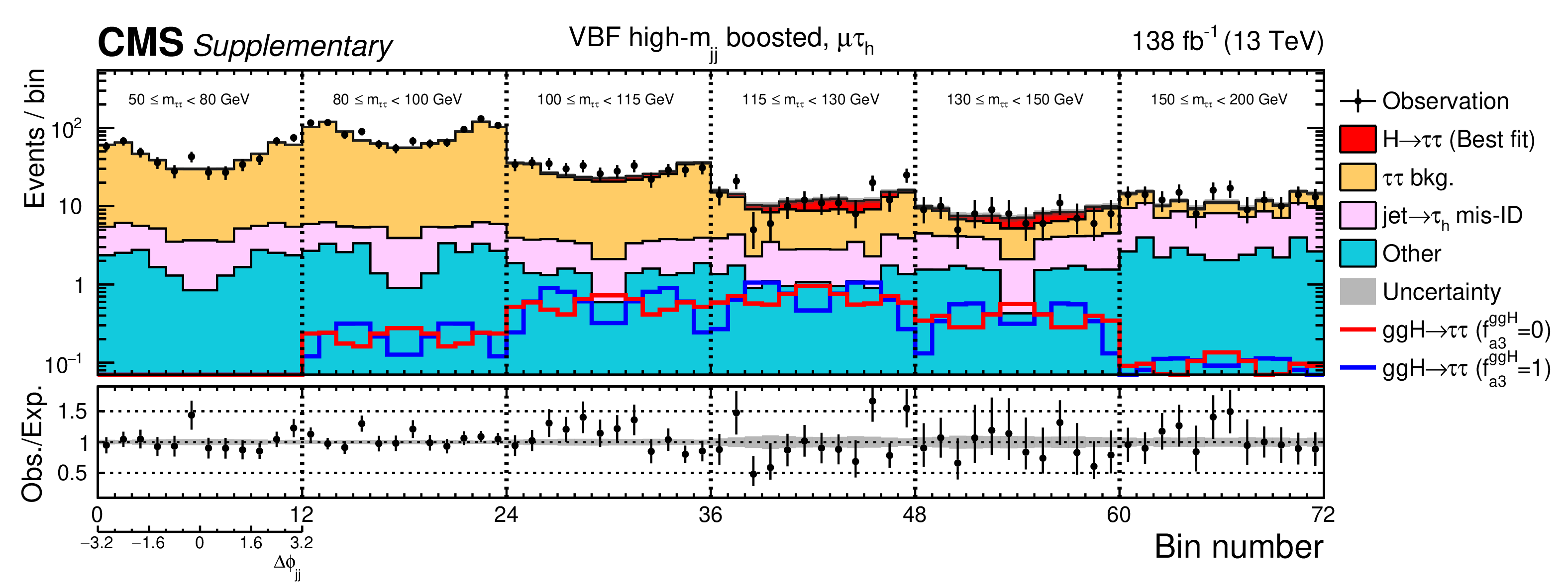
Additional Figure 1:
Observed and predicted 2D distributions after the fit to data to extract the ggH anomalous coupling parameters using the $\Delta \phi _{\mathrm {jj}}$ method for the VBF high-$m_{\mathrm {jj}}$ boosted category in the $\mu {\tau _\mathrm {h}} $ channel. The uncertainty band accounts for all sources of systematic uncertainty on the signal and background predictions. The expectation in the ratio panel is the sum of the estimated backgrounds and the best fit signal. In total 12 $\Delta \phi _{\mathrm {jj}}$ bins are used with boundaries that range from $-$3.2 to 3.2. Since the physical range of $\Delta \phi _{\mathrm {jj}}$ is between ${\pm} \pi $, the first and last bins actually only include events with 8/3 $ < |\Delta \phi _{\mathrm {jj}}| < \pi $, however, the bin range is extended to $ \pm $3.2 in the plot for visualisation. |
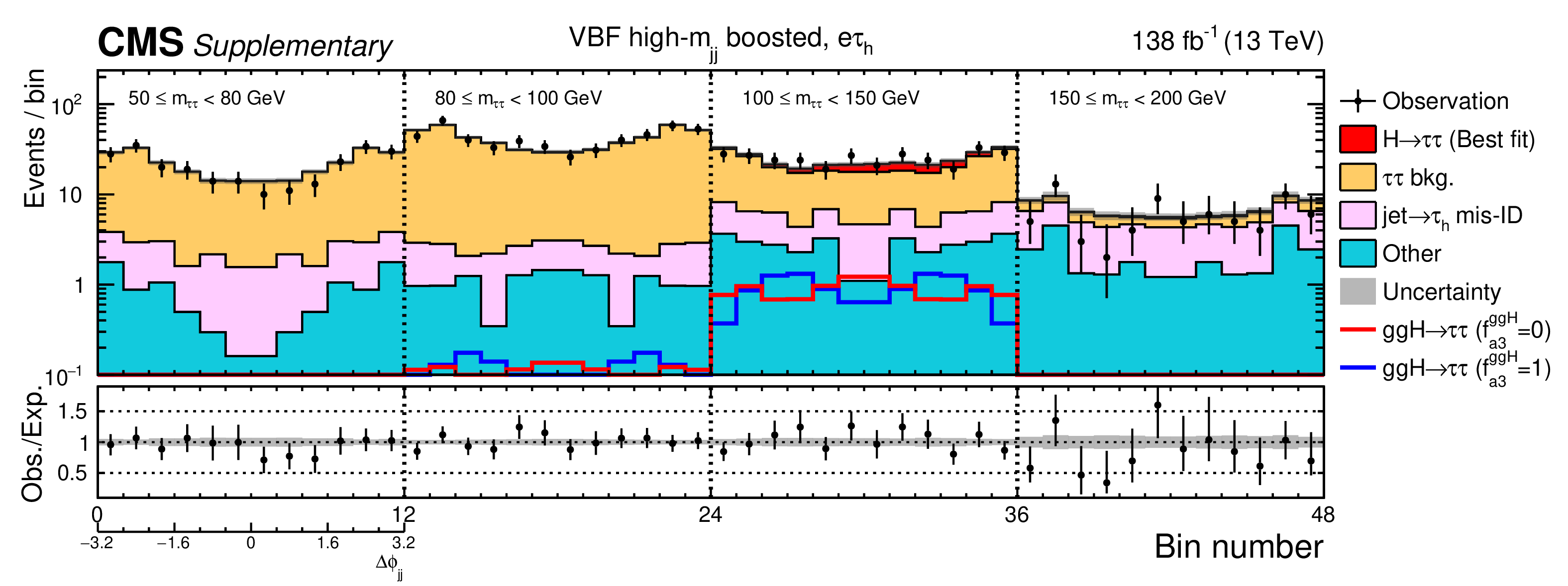
png pdf |
Additional Figure 2:
Observed and predicted 2D distributions after the fit to data to extract the ggH anomalous coupling parameters using the $\Delta \phi _{\mathrm {jj}}$ method for the VBF high-$m_{\mathrm {jj}}$ boosted category in the e$ {\tau _\mathrm {h}} $ channel. The uncertainty band accounts for all sources of systematic uncertainty on the signal and background predictions. The expectation in the ratio panel is the sum of the estimated backgrounds and the best fit signal. In total 12 $\Delta \phi _{\mathrm {jj}}$ bins are used with boundaries that range from $-$3.2 to 3.2. Since the physical range of $\Delta \phi _{\mathrm {jj}}$ is between ${\pm} \pi $, the first and last bins actually only include events with 8/3 $ < |\Delta \phi _{\mathrm {jj}}| < \pi $, however, the bin range is extended to $ \pm $3.2 in the plot for visualisation. |

png pdf |
Additional Figure 3:
Observed and predicted 2D distributions after the fit to data to extract the ggH anomalous coupling parameters using the $\Delta \phi _{\mathrm {jj}}$ method for the VBF high-$m_{\mathrm {jj}}$ boosted category in the e$ \mu $ channel. The uncertainty band accounts for all sources of systematic uncertainty on the signal and background predictions. The expectation in the ratio panel is the sum of the estimated backgrounds and the best fit signal. In total 12 $\Delta \phi _{\mathrm {jj}}$ bins are used with boundaries that range from $-$3.2 to 3.2. Since the physical range of $\Delta \phi _{\mathrm {jj}}$ is between ${\pm} \pi $, the first and last bins actually only include events with 8/3 $ < |\Delta \phi _{\mathrm {jj}}| < \pi $, however, the bin range is extended to $ \pm $3.2 in the plot for visualisation. |
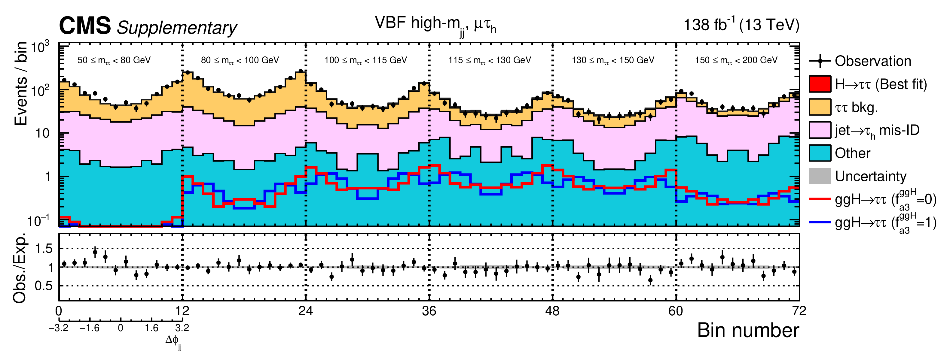
png pdf |
Additional Figure 4:
Observed and predicted 2D distributions after the fit to data to extract the ggH anomalous coupling parameters using the $\Delta \phi _{\mathrm {jj}}$ method for the VBF high-$m_{\mathrm {jj}}$ category in the $\mu {\tau _\mathrm {h}} $ channel. The uncertainty band accounts for all sources of systematic uncertainty on the signal and background predictions. The expectation in the ratio panel is the sum of the estimated backgrounds and the best fit signal. In total 12 $\Delta \phi _{\mathrm {jj}}$ bins are used with boundaries that range from $-$3.2 to 3.2. Since the physical range of $\Delta \phi _{\mathrm {jj}}$ is between ${\pm} \pi $, the first and last bins actually only include events with 8/3 $ < |\Delta \phi _{\mathrm {jj}}| < \pi $, however, the bin range is extended to $ \pm $3.2 in the plot for visualisation. |

png pdf |
Additional Figure 5:
Observed and predicted 2D distributions after the fit to data to extract the ggH anomalous coupling parameters using the $\Delta \phi _{\mathrm {jj}}$ method for the VBF high-$m_{\mathrm {jj}}$ category in the $ {\tau _\mathrm {h}} {\tau _\mathrm {h}} $ channel. The uncertainty band accounts for all sources of systematic uncertainty on the signal and background predictions. The expectation in the ratio panel is the sum of the estimated backgrounds and the best fit signal. In total 12 $\Delta \phi _{\mathrm {jj}}$ bins are used with boundaries that range from $-$3.2 to 3.2. Since the physical range of $\Delta \phi _{\mathrm {jj}}$ is between ${\pm} \pi $, the first and last bins actually only include events with 8/3 $ < |\Delta \phi _{\mathrm {jj}}| < \pi $, however, the bin range is extended to $ \pm $3.2 in the plot for visualisation. |
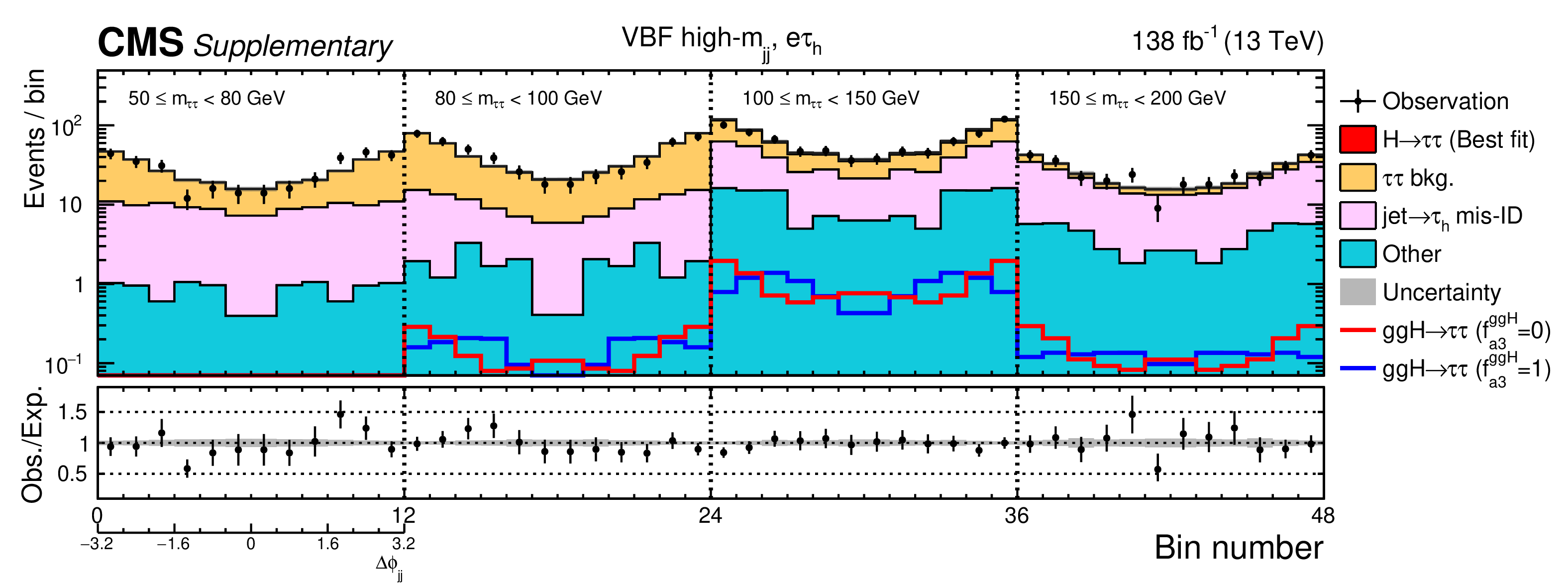
png pdf |
Additional Figure 6:
Observed and predicted 2D distributions after the fit to data to extract the ggH anomalous coupling parameters using the $\Delta \phi _{\mathrm {jj}}$ method for the VBF high-$m_{\mathrm {jj}}$ category in the e$ {\tau _\mathrm {h}} $ channel. The uncertainty band accounts for all sources of systematic uncertainty on the signal and background predictions. The expectation in the ratio panel is the sum of the estimated backgrounds and the best fit signal. In total 12 $\Delta \phi _{\mathrm {jj}}$ bins are used with boundaries that range from $-$3.2 to 3.2. Since the physical range of $\Delta \phi _{\mathrm {jj}}$ is between ${\pm} \pi $, the first and last bins actually only include events with 8/3 $ < |\Delta \phi _{\mathrm {jj}}| < \pi $, however, the bin range is extended to $ \pm $3.2 in the plot for visualisation. |

png pdf |
Additional Figure 7:
Observed and predicted 2D distributions after the fit to data to extract the ggH anomalous coupling parameters using the $\Delta \phi _{\mathrm {jj}}$ method for the VBF high-$m_{\mathrm {jj}}$ category in the e$ \mu $ channel. The uncertainty band accounts for all sources of systematic uncertainty on the signal and background predictions. The expectation in the ratio panel is the sum of the estimated backgrounds and the best fit signal. In total 12 $\Delta \phi _{\mathrm {jj}}$ bins are used with boundaries that range from $-$3.2 to 3.2. Since the physical range of $\Delta \phi _{\mathrm {jj}}$ is between ${\pm} \pi $, the first and last bins actually only include events with 8/3 $ < |\Delta \phi _{\mathrm {jj}}| < \pi $, however, the bin range is extended to $ \pm $3.2 in the plot for visualisation. |
png pdf |
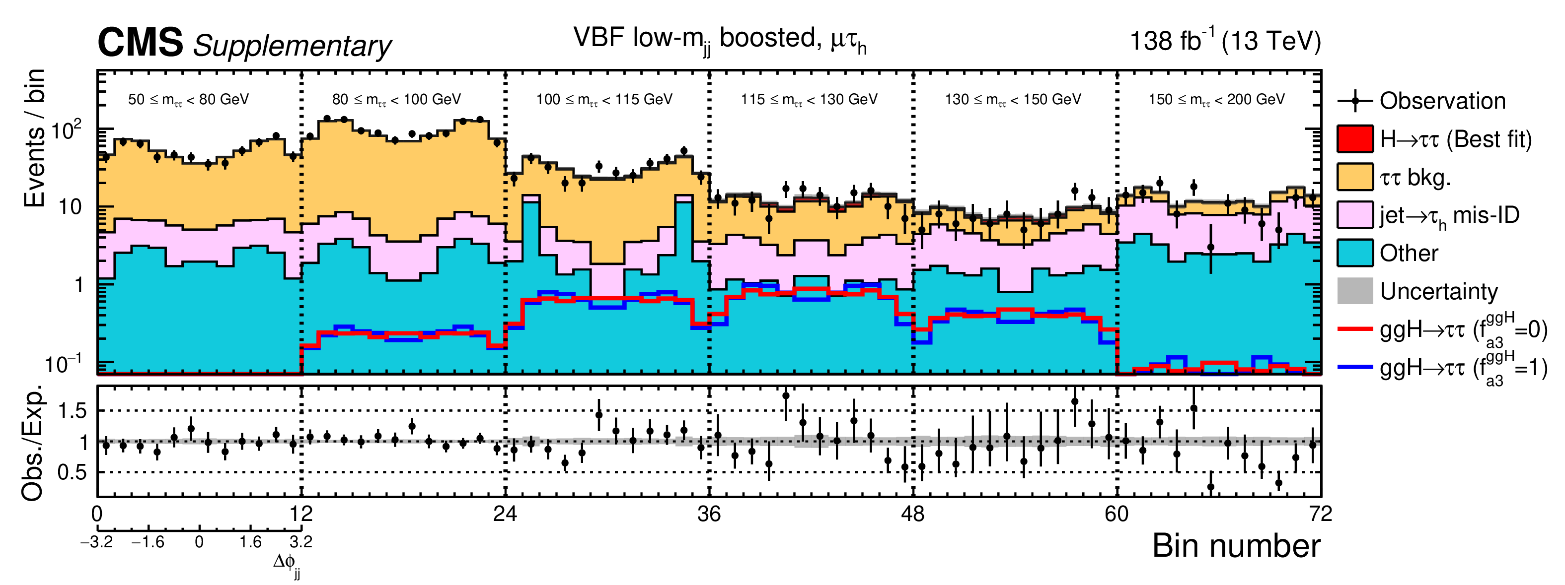
Additional Figure 8:
Observed and predicted 2D distributions after the fit to data to extract the ggH anomalous coupling parameters using the $\Delta \phi _{\mathrm {jj}}$ method for the VBF low-$m_{\mathrm {jj}}$ boosted category in the $\mu {\tau _\mathrm {h}} $ channel. The uncertainty band accounts for all sources of systematic uncertainty on the signal and background predictions. The expectation in the ratio panel is the sum of the estimated backgrounds and the best fit signal. In total 12 $\Delta \phi _{\mathrm {jj}}$ bins are used with boundaries that range from $-$3.2 to 3.2. Since the physical range of $\Delta \phi _{\mathrm {jj}}$ is between ${\pm} \pi $, the first and last bins actually only include events with 8/3 $ < |\Delta \phi _{\mathrm {jj}}| < \pi $, however, the bin range is extended to $ \pm $3.2 in the plot for visualisation. |
png pdf |
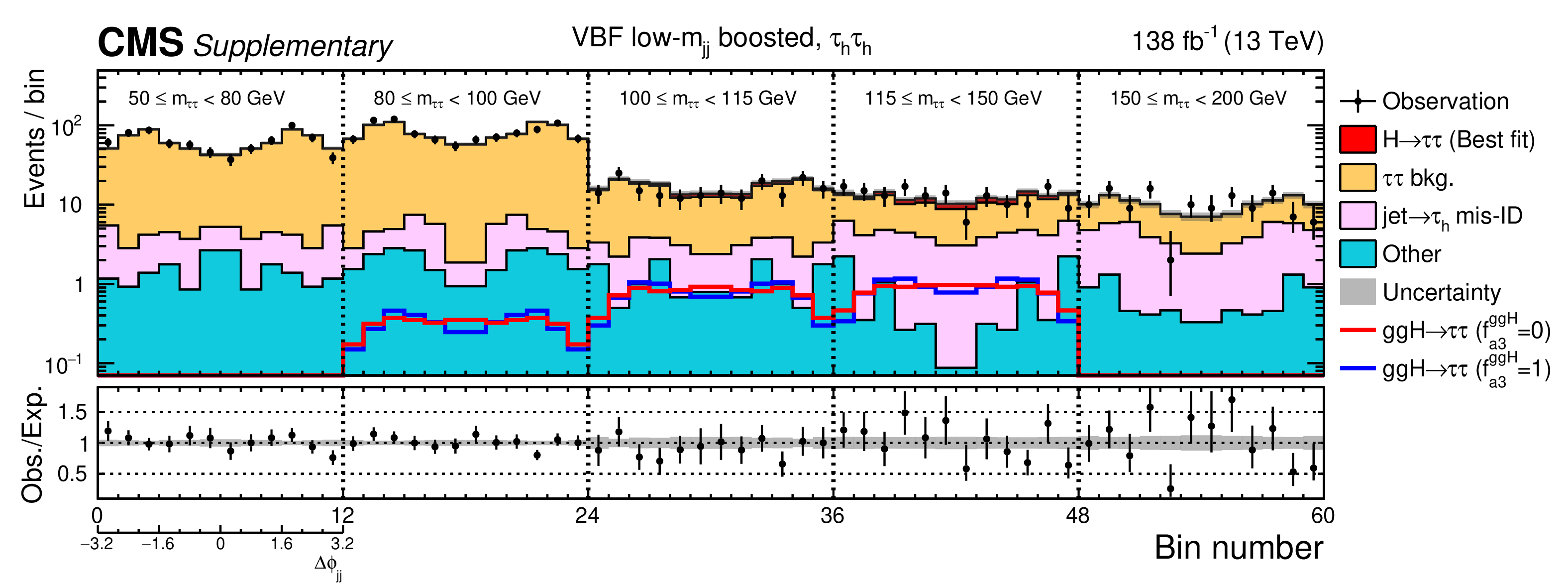
Additional Figure 9:
Observed and predicted 2D distributions after the fit to data to extract the ggH anomalous coupling parameters using the $\Delta \phi _{\mathrm {jj}}$ method for the VBF low-$m_{\mathrm {jj}}$ boosted category in the $ {\tau _\mathrm {h}} {\tau _\mathrm {h}} $ channel. The uncertainty band accounts for all sources of systematic uncertainty on the signal and background predictions. The expectation in the ratio panel is the sum of the estimated backgrounds and the best fit signal. In total 12 $\Delta \phi _{\mathrm {jj}}$ bins are used with boundaries that range from $-$3.2 to 3.2. Since the physical range of $\Delta \phi _{\mathrm {jj}}$ is between ${\pm} \pi $, the first and last bins actually only include events with 8/3 $ < |\Delta \phi _{\mathrm {jj}}| < \pi $, however, the bin range is extended to $ \pm $3.2 in the plot for visualisation. |
png pdf |
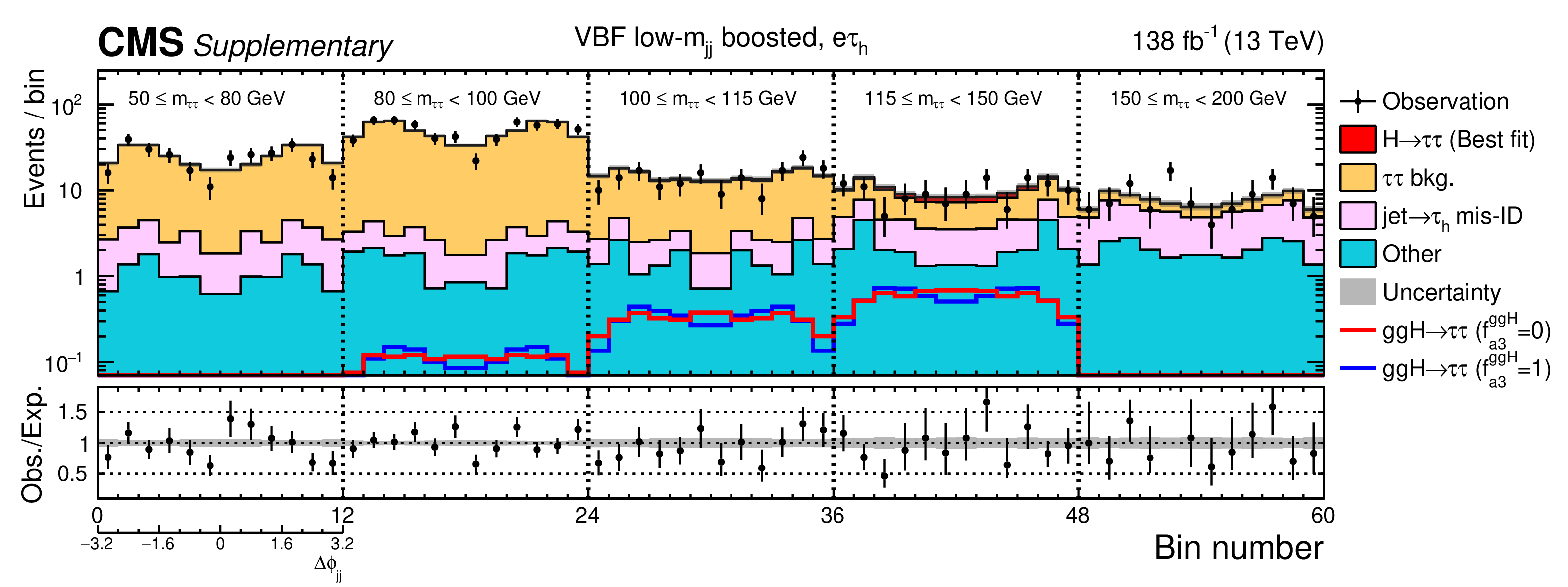
Additional Figure 10:
Observed and predicted 2D distributions after the fit to data to extract the ggH anomalous coupling parameters using the $\Delta \phi _{\mathrm {jj}}$ method for the VBF low-$m_{\mathrm {jj}}$ boosted category in the e$ {\tau _\mathrm {h}} $ channel. The uncertainty band accounts for all sources of systematic uncertainty on the signal and background predictions. The expectation in the ratio panel is the sum of the estimated backgrounds and the best fit signal. In total 12 $\Delta \phi _{\mathrm {jj}}$ bins are used with boundaries that range from $-$3.2 to 3.2. Since the physical range of $\Delta \phi _{\mathrm {jj}}$ is between ${\pm} \pi $, the first and last bins actually only include events with 8/3 $ < |\Delta \phi _{\mathrm {jj}}| < \pi $, however, the bin range is extended to $ \pm $3.2 in the plot for visualisation. |

png pdf |
Additional Figure 11:
Observed and predicted 2D distributions after the fit to data to extract the ggH anomalous coupling parameters using the $\Delta \phi _{\mathrm {jj}}$ method for the VBF low-$m_{\mathrm {jj}}$ boosted category in the e$ \mu $ channel. The uncertainty band accounts for all sources of systematic uncertainty on the signal and background predictions. The expectation in the ratio panel is the sum of the estimated backgrounds and the best fit signal. In total 12 $\Delta \phi _{\mathrm {jj}}$ bins are used with boundaries that range from $-$3.2 to 3.2. Since the physical range of $\Delta \phi _{\mathrm {jj}}$ is between ${\pm} \pi $, the first and last bins actually only include events with 8/3 $ < |\Delta \phi _{\mathrm {jj}}| < \pi $, however, the bin range is extended to $ \pm $3.2 in the plot for visualisation. |

png pdf |
Additional Figure 12:
Observed and predicted 2D distributions after the fit to data to extract the ggH anomalous coupling parameters using the $\Delta \phi _{\mathrm {jj}}$ method for the VBF low-$m_{\mathrm {jj}}$ category in the $\mu {\tau _\mathrm {h}} $ channel. The uncertainty band accounts for all sources of systematic uncertainty on the signal and background predictions. The expectation in the ratio panel is the sum of the estimated backgrounds and the best fit signal. In total 12 $\Delta \phi _{\mathrm {jj}}$ bins are used with boundaries that range from $-$3.2 to 3.2. Since the physical range of $\Delta \phi _{\mathrm {jj}}$ is between ${\pm} \pi $, the first and last bins actually only include events with 8/3 $ < |\Delta \phi _{\mathrm {jj}}| < \pi $, however, the bin range is extended to $ \pm $3.2 in the plot for visualisation. |
png pdf |
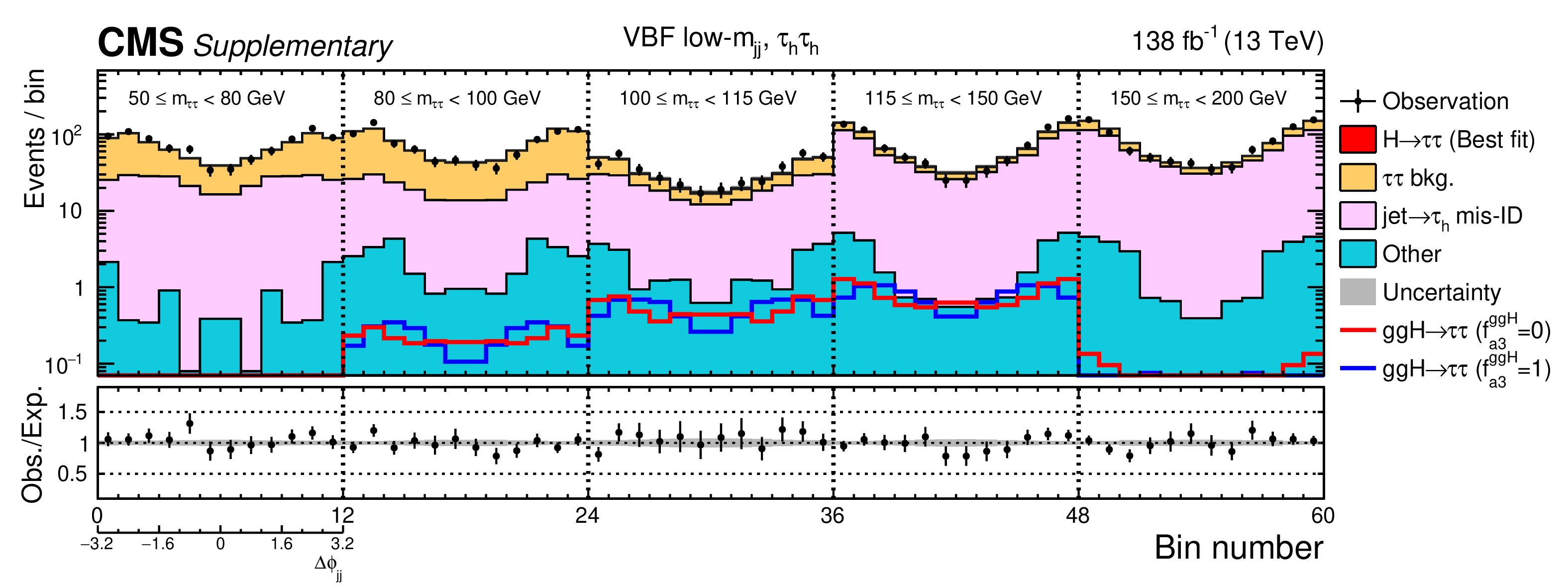
Additional Figure 13:
Observed and predicted 2D distributions after the fit to data to extract the ggH anomalous coupling parameters using the $\Delta \phi _{\mathrm {jj}}$ method for the VBF low-$m_{\mathrm {jj}}$ category in the $ {\tau _\mathrm {h}} {\tau _\mathrm {h}} $ channel. The uncertainty band accounts for all sources of systematic uncertainty on the signal and background predictions. The expectation in the ratio panel is the sum of the estimated backgrounds and the best fit signal. In total 12 $\Delta \phi _{\mathrm {jj}}$ bins are used with boundaries that range from $-$3.2 to 3.2. Since the physical range of $\Delta \phi _{\mathrm {jj}}$ is between ${\pm} \pi $, the first and last bins actually only include events with 8/3 $ < |\Delta \phi _{\mathrm {jj}}| < \pi $, however, the bin range is extended to $ \pm $3.2 in the plot for visualisation. |
png pdf |
Additional Figure 14:
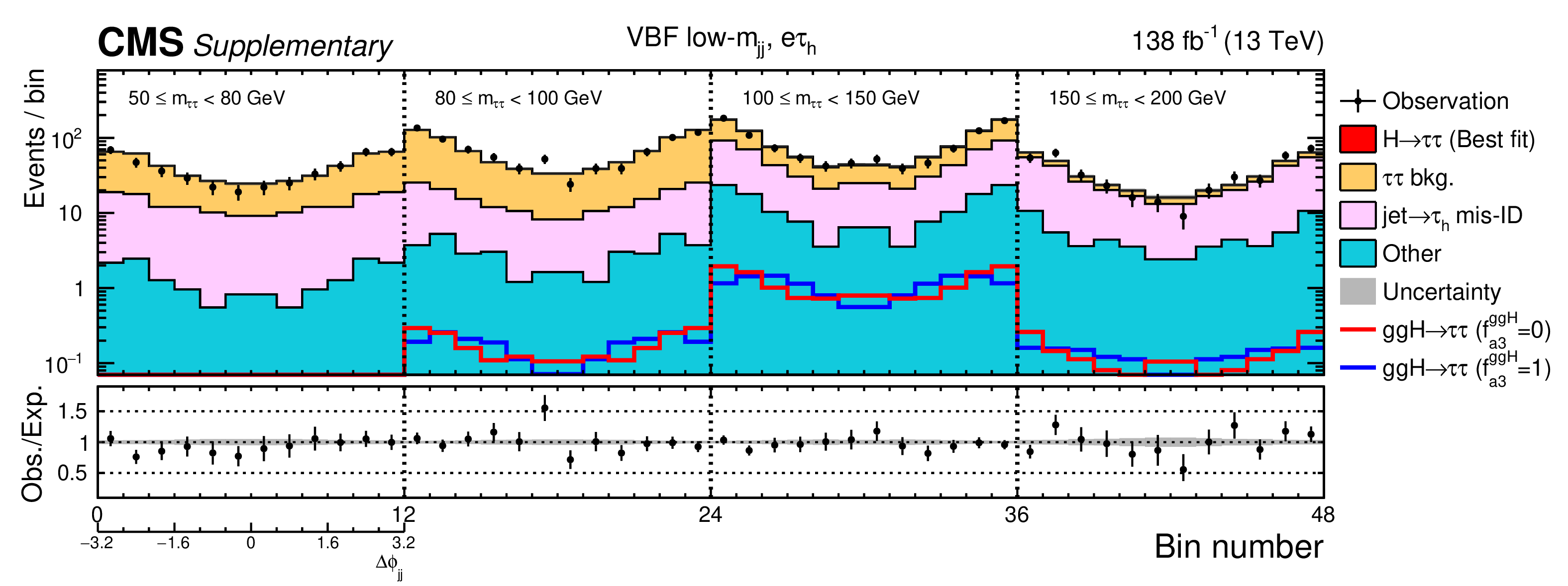
Observed and predicted 2D distributions after the fit to data to extract the ggH anomalous coupling parameters using the $\Delta \phi _{\mathrm {jj}}$ method for the VBF low-$m_{\mathrm {jj}}$ category in the e$ {\tau _\mathrm {h}} $ channel. The uncertainty band accounts for all sources of systematic uncertainty on the signal and background predictions. The expectation in the ratio panel is the sum of the estimated backgrounds and the best fit signal. In total 12 $\Delta \phi _{\mathrm {jj}}$ bins are used with boundaries that range from $-$3.2 to 3.2. Since the physical range of $\Delta \phi _{\mathrm {jj}}$ is between ${\pm} \pi $, the first and last bins actually only include events with 8/3 $ < |\Delta \phi _{\mathrm {jj}}| < \pi $, however, the bin range is extended to $ \pm $3.2 in the plot for visualisation. |

png pdf |
Additional Figure 15:
Observed and predicted 2D distributions after the fit to data to extract the ggH anomalous coupling parameters using the $\Delta \phi _{\mathrm {jj}}$ method for the VBF low-$m_{\mathrm {jj}}$ category in the e$ \mu $ channel. The uncertainty band accounts for all sources of systematic uncertainty on the signal and background predictions. The expectation in the ratio panel is the sum of the estimated backgrounds and the best fit signal. In total 12 $\Delta \phi _{\mathrm {jj}}$ bins are used with boundaries that range from $-$3.2 to 3.2. Since the physical range of $\Delta \phi _{\mathrm {jj}}$ is between ${\pm} \pi $, the first and last bins actually only include events with 8/3 $ < |\Delta \phi _{\mathrm {jj}}| < \pi $, however, the bin range is extended to $ \pm $3.2 in the plot for visualisation. |
png pdf |
Additional Figure 16:
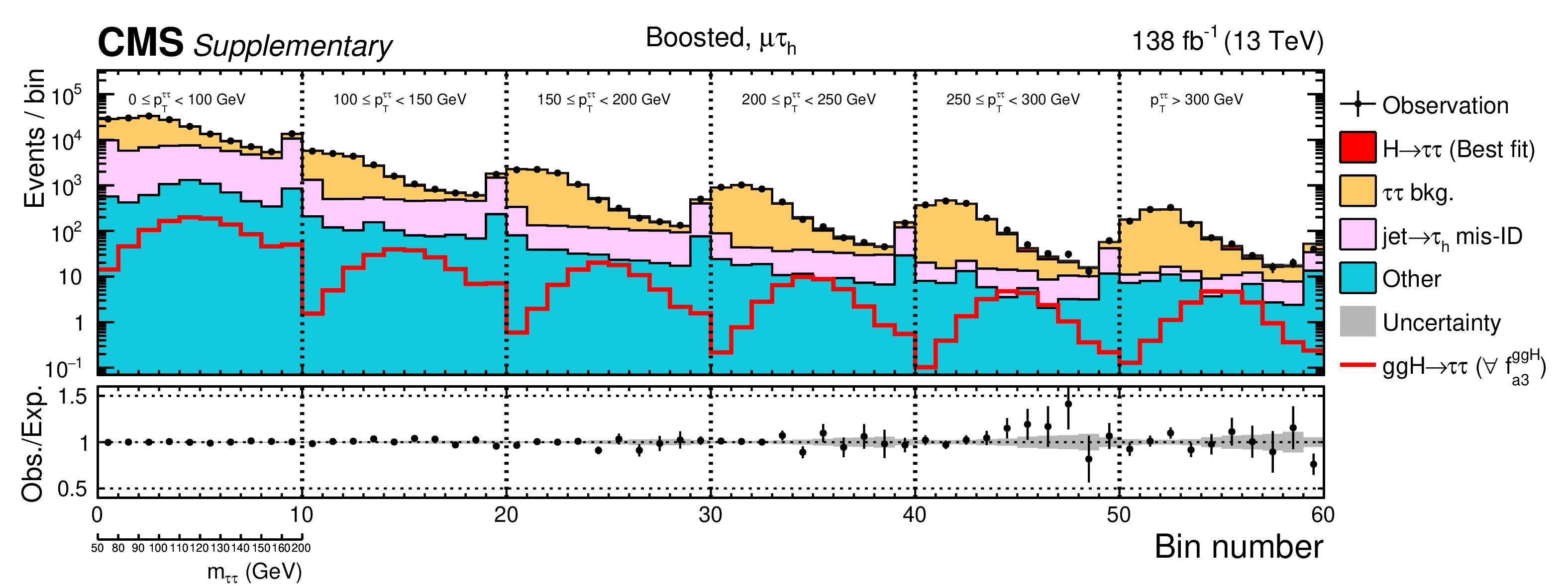
Observed and predicted 2D distributions after the fit to data to extract the ggH anomalous coupling parameters using the $\Delta \phi _{\mathrm {jj}}$ method for the boosted category in the $\mu {\tau _\mathrm {h}} $ channel. The uncertainty band accounts for all sources of systematic uncertainty on the signal and background predictions. The expectation in the ratio panel is the sum of the estimated backgrounds and the best fit signal. |
png pdf |
Additional Figure 17:
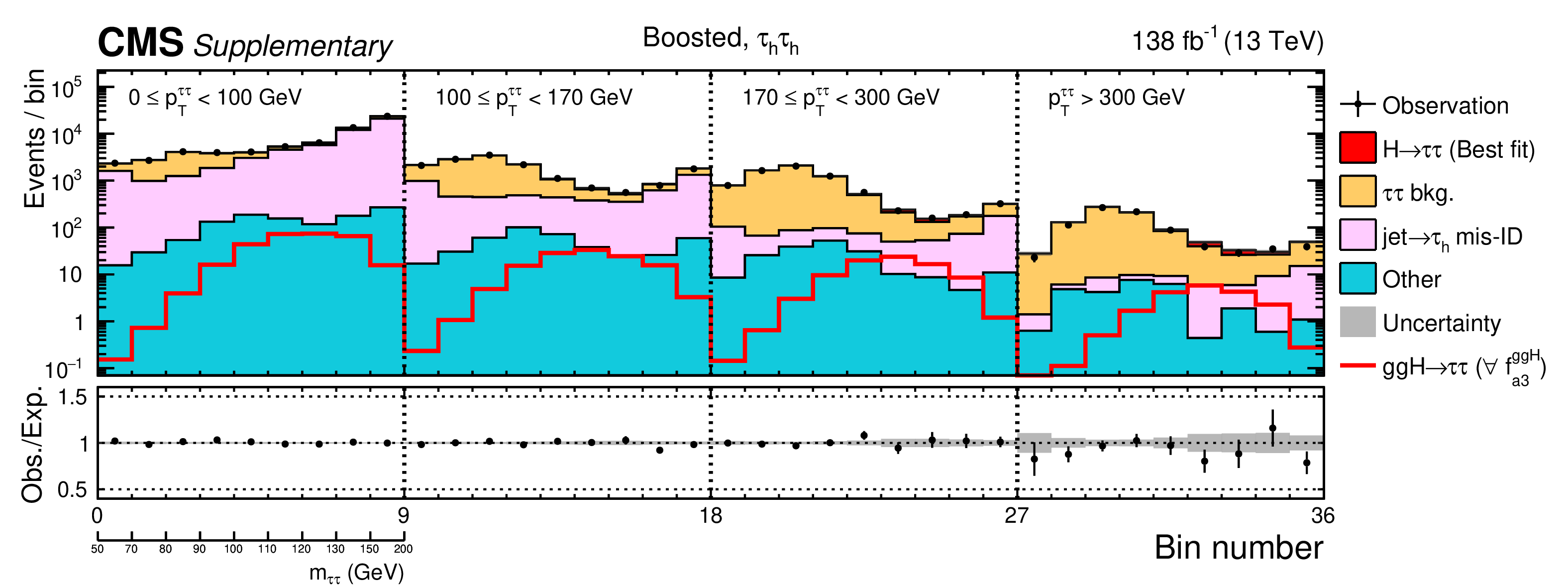
Observed and predicted 2D distributions after the fit to data to extract the ggH anomalous coupling parameters using the $\Delta \phi _{\mathrm {jj}}$ method for the boosted category in the $ {\tau _\mathrm {h}} {\tau _\mathrm {h}} $ channel. The uncertainty band accounts for all sources of systematic uncertainty on the signal and background predictions. The expectation in the ratio panel is the sum of the estimated backgrounds and the best fit signal. |
png pdf |
Additional Figure 18:
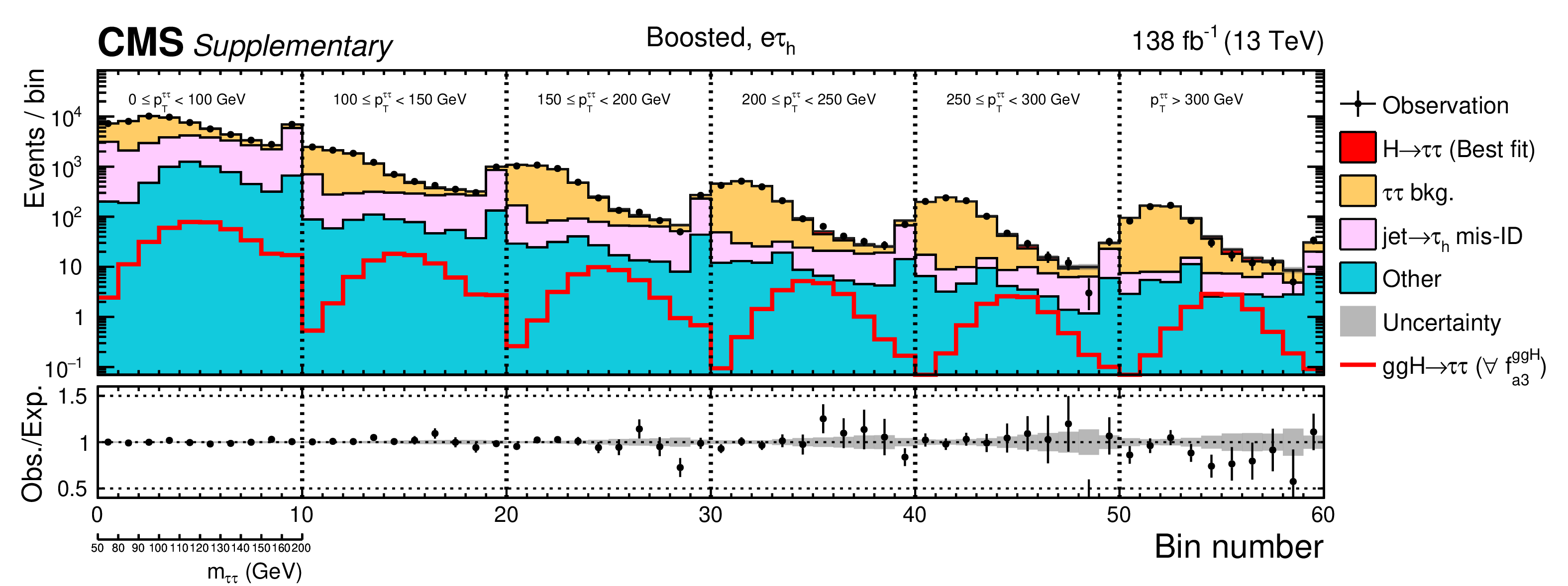
Observed and predicted 2D distributions after the fit to data to extract the ggH anomalous coupling parameters using the $\Delta \phi _{\mathrm {jj}}$ method for the boosted category in the e$ {\tau _\mathrm {h}} $ channel. The uncertainty band accounts for all sources of systematic uncertainty on the signal and background predictions. The expectation in the ratio panel is the sum of the estimated backgrounds and the best fit signal. |
png pdf |
Additional Figure 19:
Observed and predicted 2D distributions after the fit to data to extract the ggH anomalous coupling parameters using the $\Delta \phi _{\mathrm {jj}}$ method for the boosted category in the e$ \mu $ channel. The uncertainty band accounts for all sources of systematic uncertainty on the signal and background predictions. The expectation in the ratio panel is the sum of the estimated backgrounds and the best fit signal. |
png pdf |
Additional Figure 20:
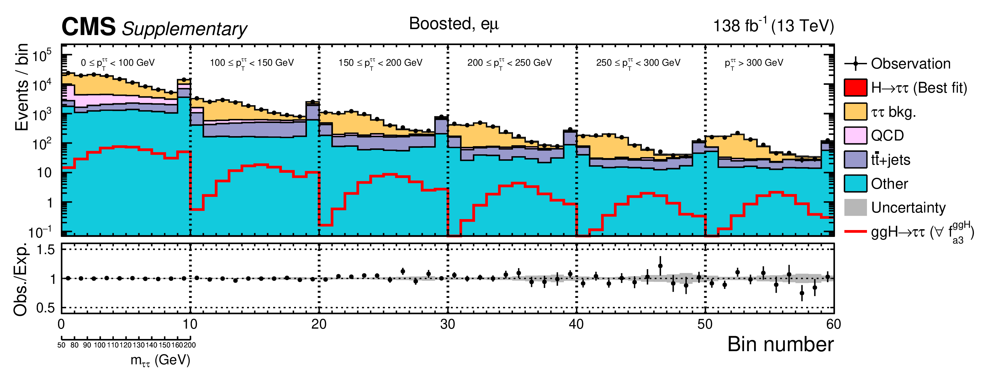
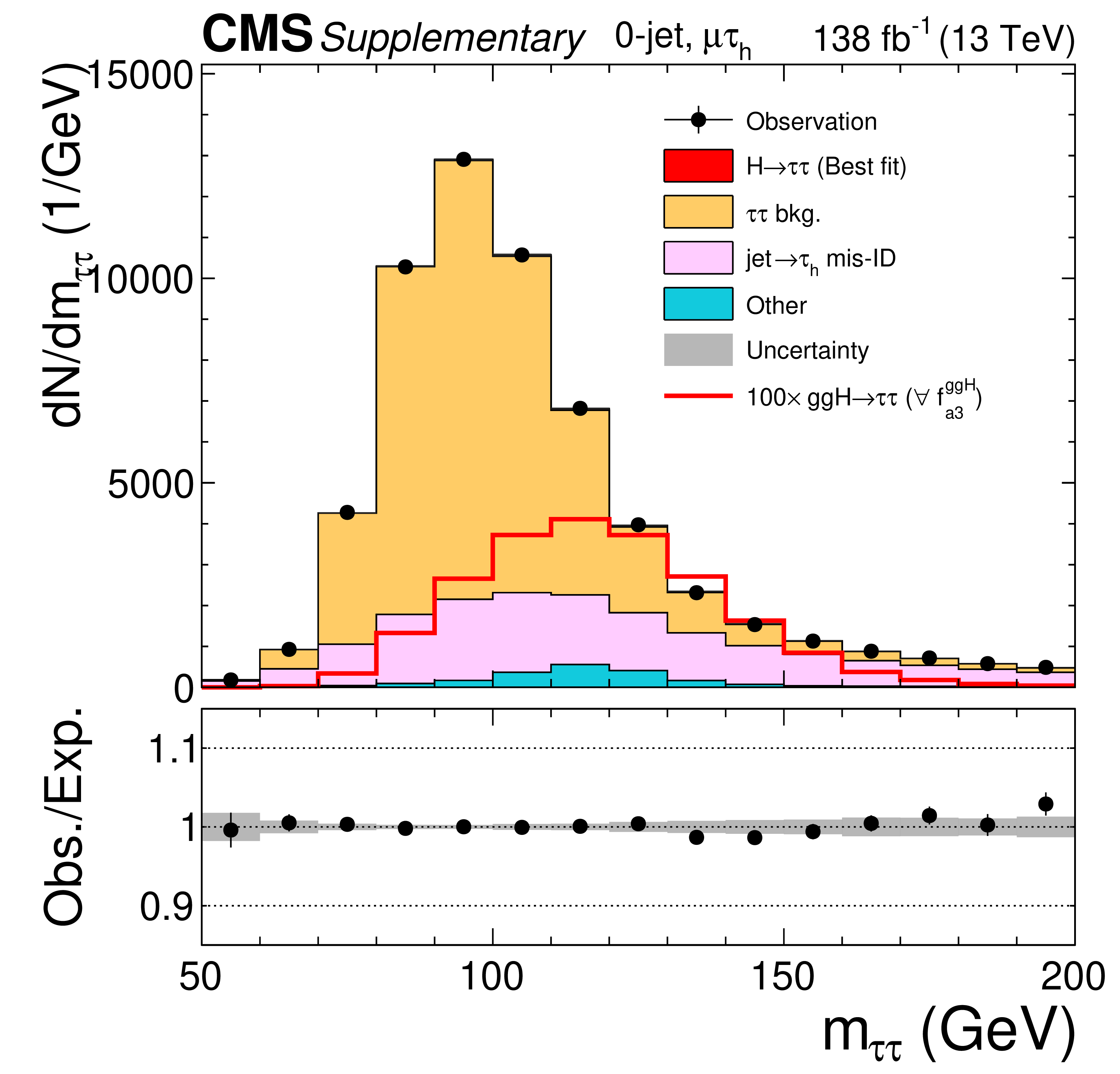
Observed and predicted $m_{\tau \tau}$ distributions after the fit to data to extract the ggH anomalous coupling parameters using the $\Delta \phi _{\mathrm {jj}}$ method for the 0-jet category in the $\mu {\tau _\mathrm {h}} $ channel. The uncertainty band accounts for all sources of systematic uncertainty on the signal and background predictions. The expectation in the ratio panel is the sum of the estimated backgrounds and the best fit signal. |
png pdf |
Additional Figure 21:
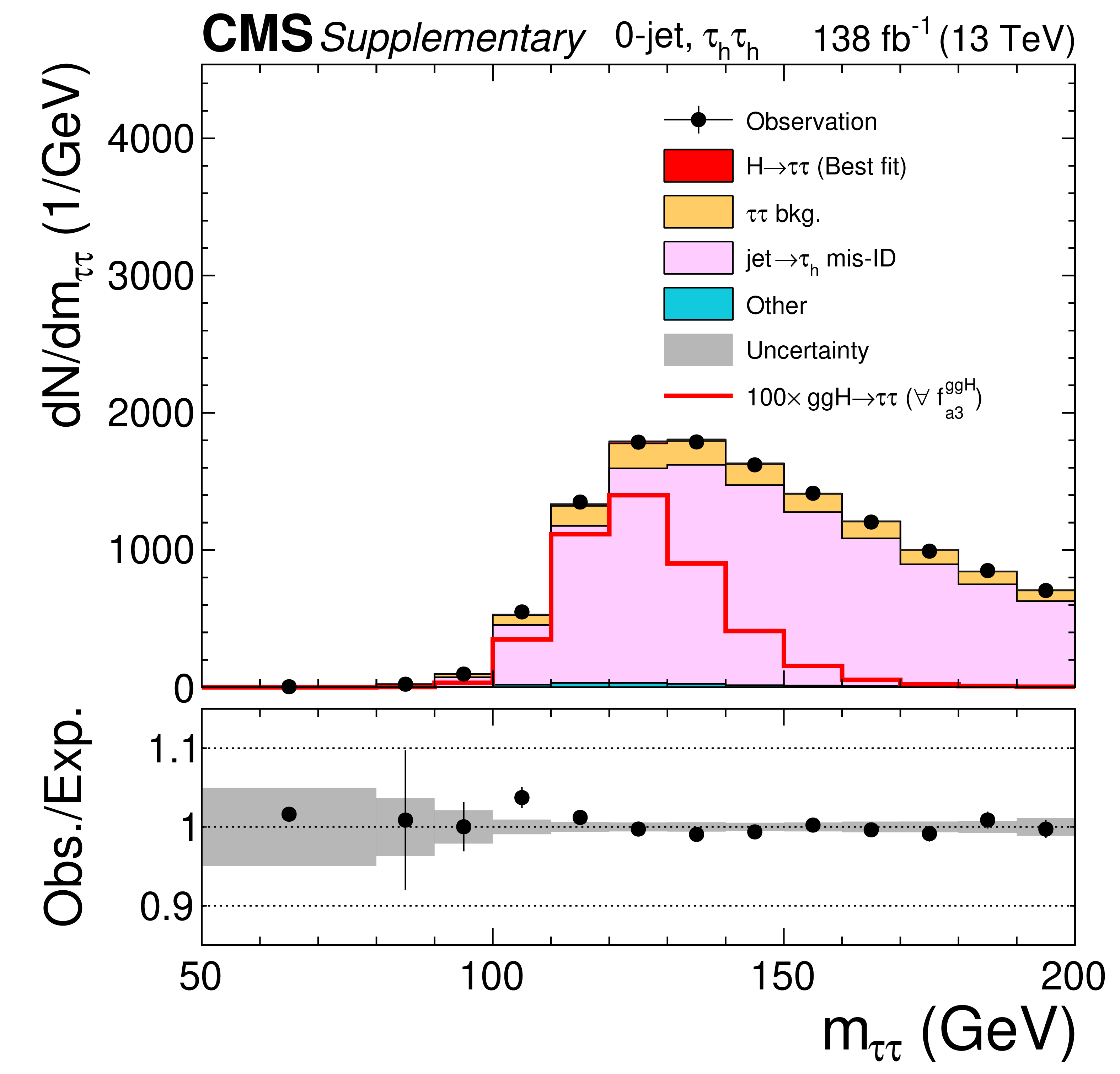
Observed and predicted $m_{\tau \tau}$ distributions after the fit to data to extract the ggH anomalous coupling parameters using the $\Delta \phi _{\mathrm {jj}}$ method for the 0-jet category in the $ {\tau _\mathrm {h}} {\tau _\mathrm {h}} $ channel. The uncertainty band accounts for all sources of systematic uncertainty on the signal and background predictions. The expectation in the ratio panel is the sum of the estimated backgrounds and the best fit signal. |
png pdf |
Additional Figure 22:
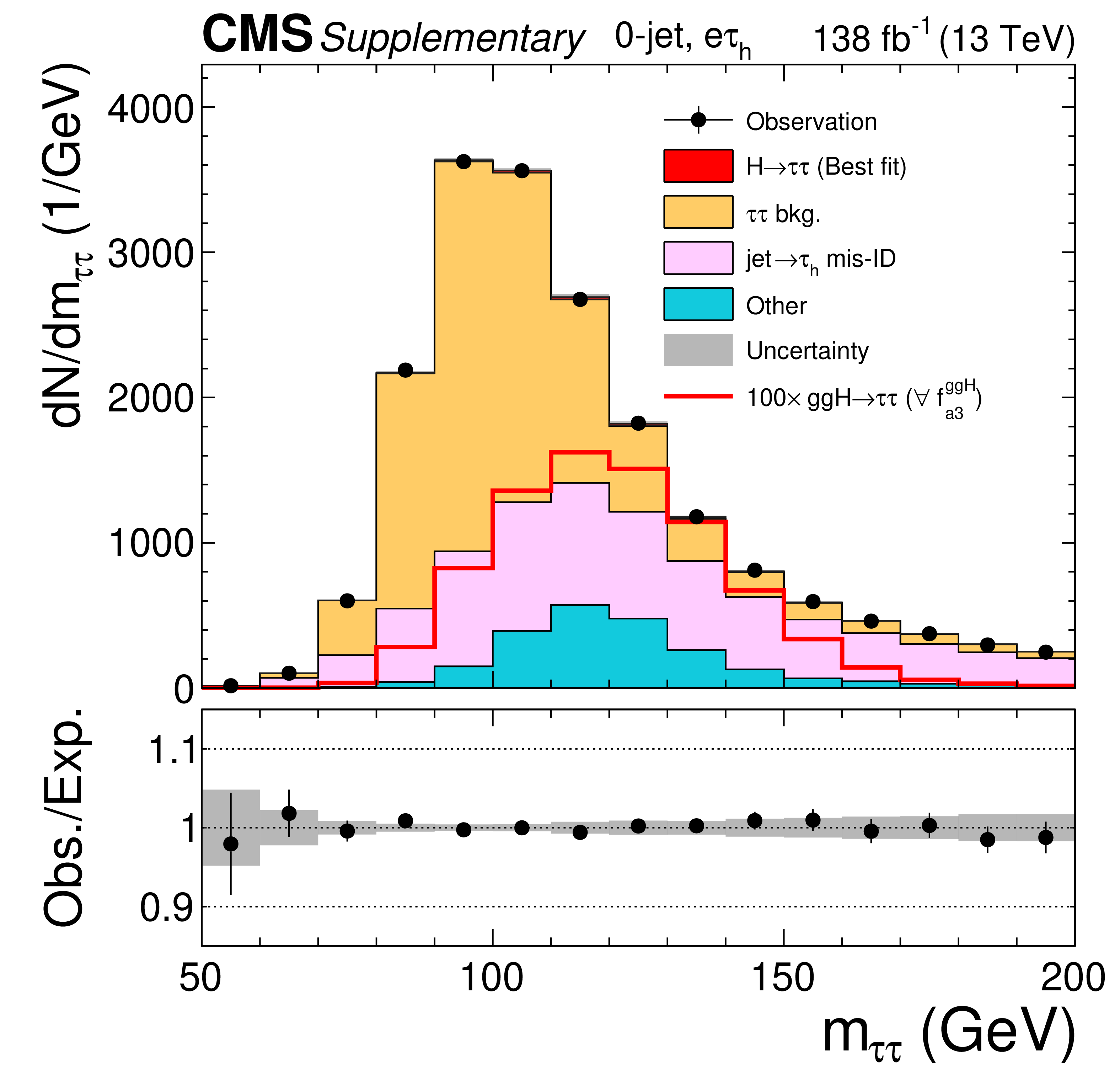
Observed and predicted $m_{\tau \tau}$ distributions after the fit to data to extract the ggH anomalous coupling parameters using the $\Delta \phi _{\mathrm {jj}}$ method for the 0-jet category in the e$ {\tau _\mathrm {h}} $ channel. The uncertainty band accounts for all sources of systematic uncertainty on the signal and background predictions. The expectation in the ratio panel is the sum of the estimated backgrounds and the best fit signal. |

png pdf |
Additional Figure 23:
Observed and predicted $m_{\tau \tau}$ distributions after the fit to data to extract the ggH anomalous coupling parameters using the $\Delta \phi _{\mathrm {jj}}$ method for the VBF 0-jet category in the e$ \mu $ channel. The uncertainty band accounts for all sources of systematic uncertainty on the signal and background predictions. The expectation in the ratio panel is the sum of the estimated backgrounds and the best fit signal. |
png pdf |
Additional Figure 24:
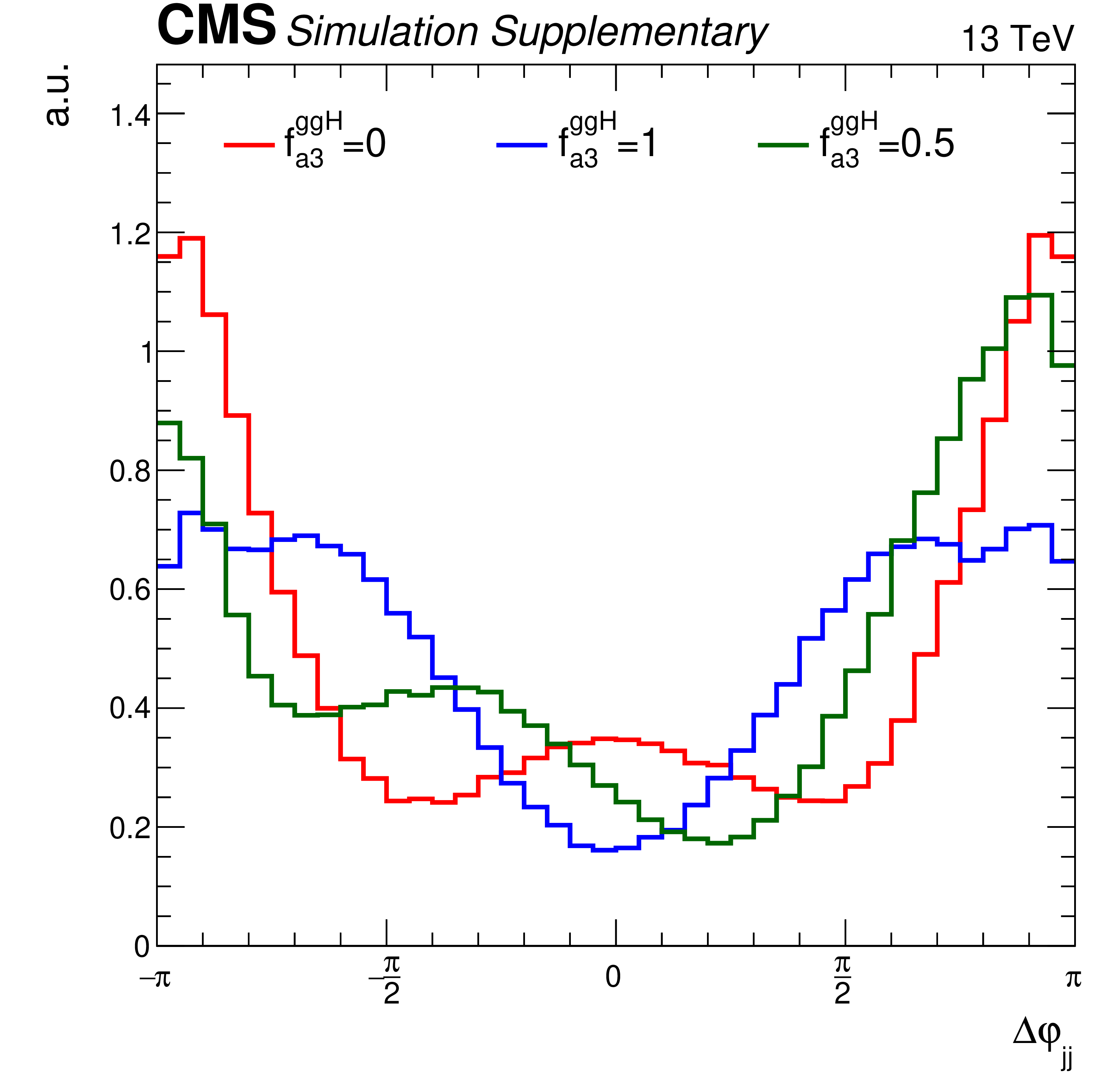
Generator-level $\Delta \phi _{\mathrm {jj}}$ distributions for ggH+2j events with $m_{\mathrm {jj}} > $ 500 GeV. The distributions are shown for a scalar Higgs ($f_{a3}^{\mathrm{g} \mathrm{g} \mathrm{H}}=$ 0) in red, a pseudoscalar Higgs ($f_{a3}^{\mathrm{g} \mathrm{g} \mathrm{H}}=$ 1) in blue, and for a CP-violating scenario with maximum-mixing between CP-even and CP-odd couplings ($f_{a3}^{\mathrm{g} \mathrm{g} \mathrm{H}}=$ 0.5) in green. |
png pdf |
Additional Figure 25:
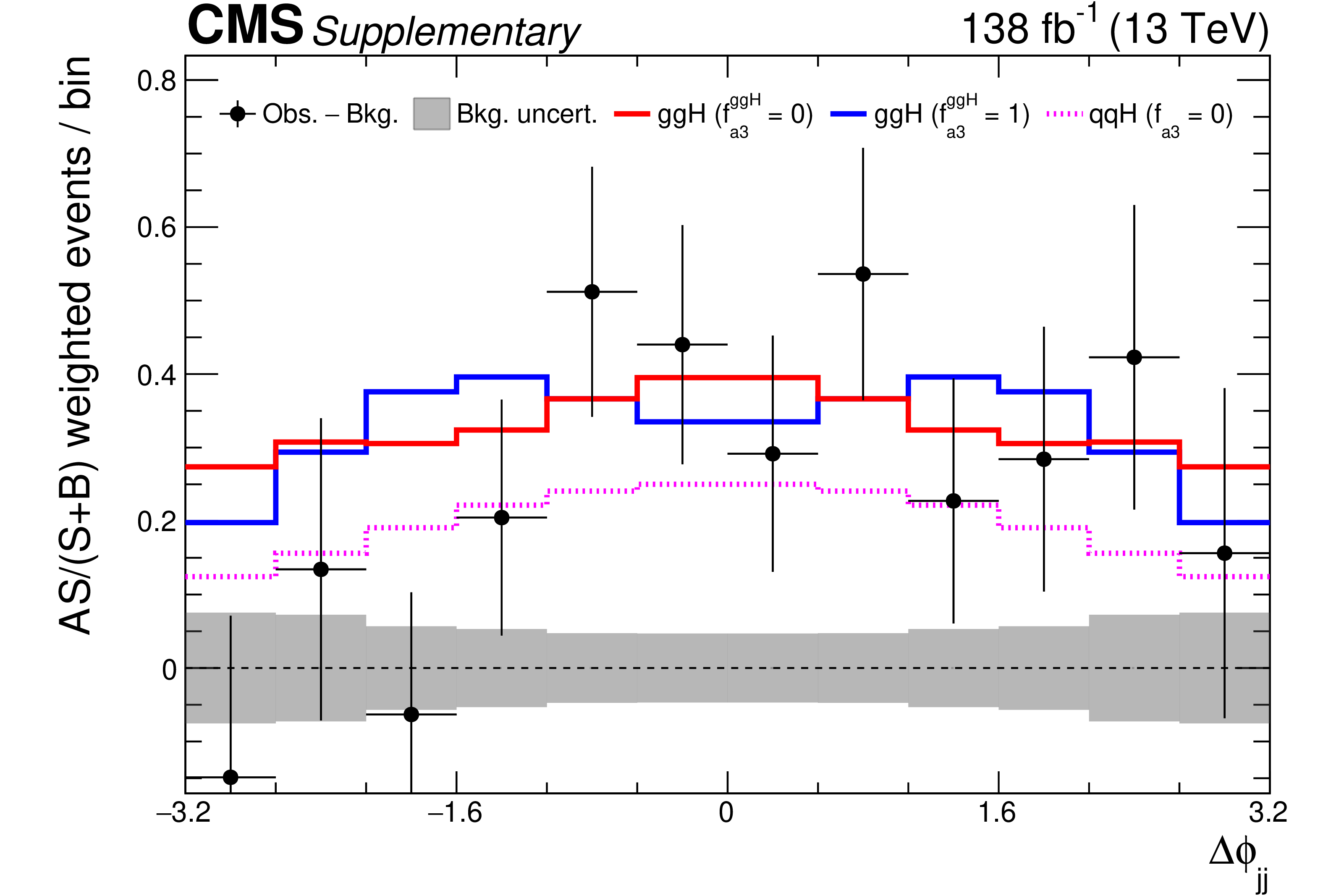
The $\Delta \phi _{\mathrm {jj}}$ distribution for all channels combined. Events were collected from all years and $m_{\tau \tau}$ bins in the four VBF signal categories. The non- $\mathrm{H} \rightarrow \tau \tau $ background is subtracted from the data. The events are reweighed by $A\,S/(S+B)$, in which $S$ and $B$ are the ggH signal and background rates, respectively, and $A$ is a measure for the average asymmetry between the scalar ($f_{a3}^{\mathrm{g} \mathrm{g} \mathrm{H}}=$ 0) and pseudoscalar ($f_{a3}^{\mathrm{g} \mathrm{g} \mathrm{H}}=$ 1) distributions. The definition of the value of $A$ per bin is $|N(f_{a3}^{\mathrm{g} \mathrm{g} \mathrm{H}}=0) - N(f_{a3}^{\mathrm{g} \mathrm{g} \mathrm{H}}=1)|/|N(f_{a3}^{\mathrm{g} \mathrm{g} \mathrm{H}}=0) + N(f_{a3}^{\mathrm{g} \mathrm{g} \mathrm{H}}=1)|$ where $N(f_{a3}^{\mathrm{g} \mathrm{g} \mathrm{H}}=0)$ and $N(f_{a3}^{\mathrm{g} \mathrm{g} \mathrm{H}}=1)$ are the expected scalar and pseudoscalar events per bin respectively, and $A$ is normalised to the total number of bins. The scalar ggH distribution is depicted in red, while the pseudoscalar ggH is displayed in blue; both are shown stacked on top of the scalar ($f_{a3}=$ 0) $\mathrm{q} \mathrm{q} \mathrm{H} $ (VBF+$\mathrm{V} \mathrm{H} $) distribution shown by the dashed magenta line. In the predictions, the rate parameters are taken from their best fit values. The grey uncertainty band indicates the uncertainty on the subtracted background component. In total 12 $\Delta \phi _{\mathrm {jj}}$ bins are used with boundaries that range from $-$3.2 to 3.2. Since the physical range of $\Delta \phi _{\mathrm {jj}}$ is between ${\pm} \pi $, the first and last bins actually only include events with 8/3 $ < |\Delta \phi _{\mathrm {jj}}| < \pi $, however, the bin range is extended to $ \pm $3.2 in the plot for visualisation. |
png pdf |
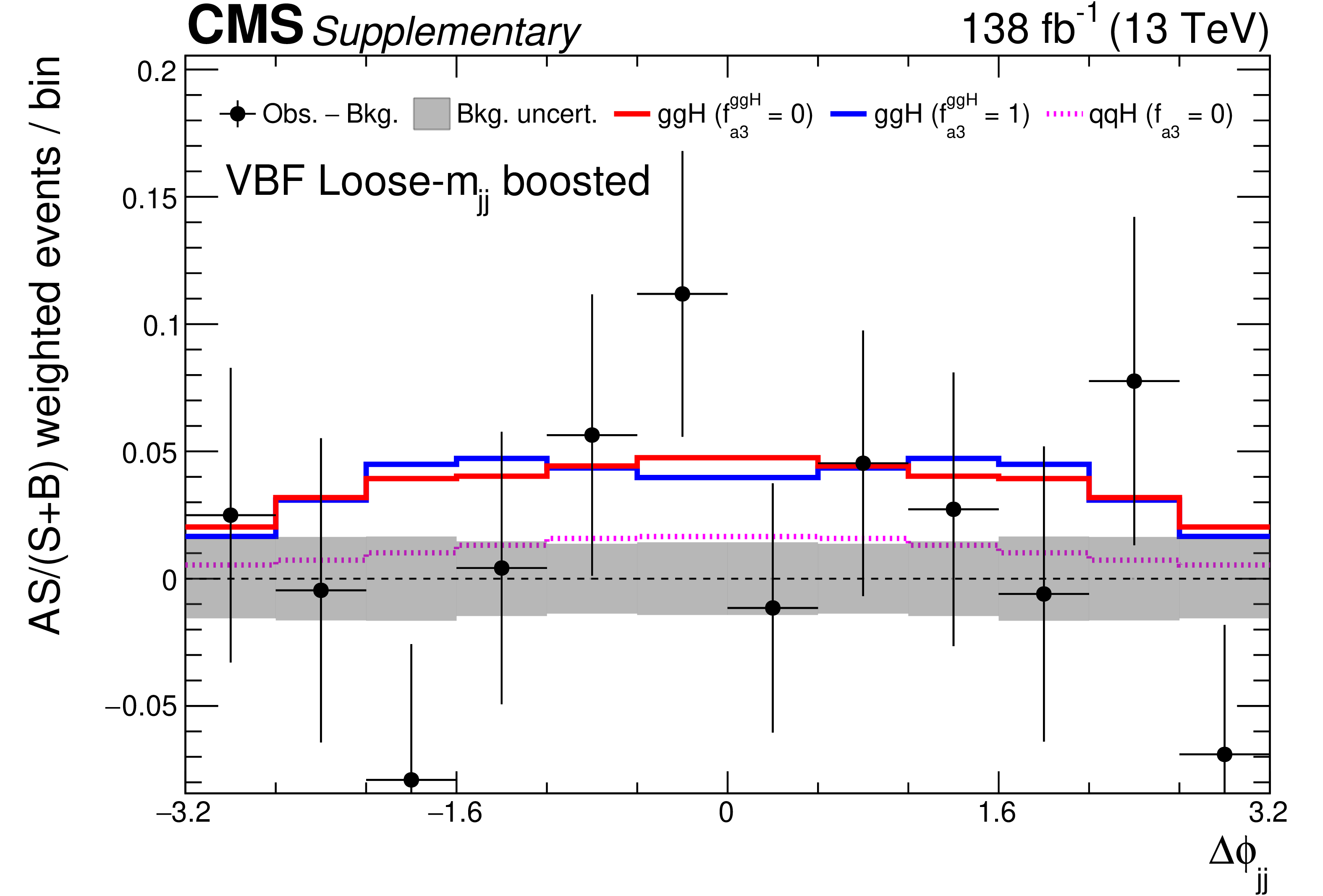
Additional Figure 26:
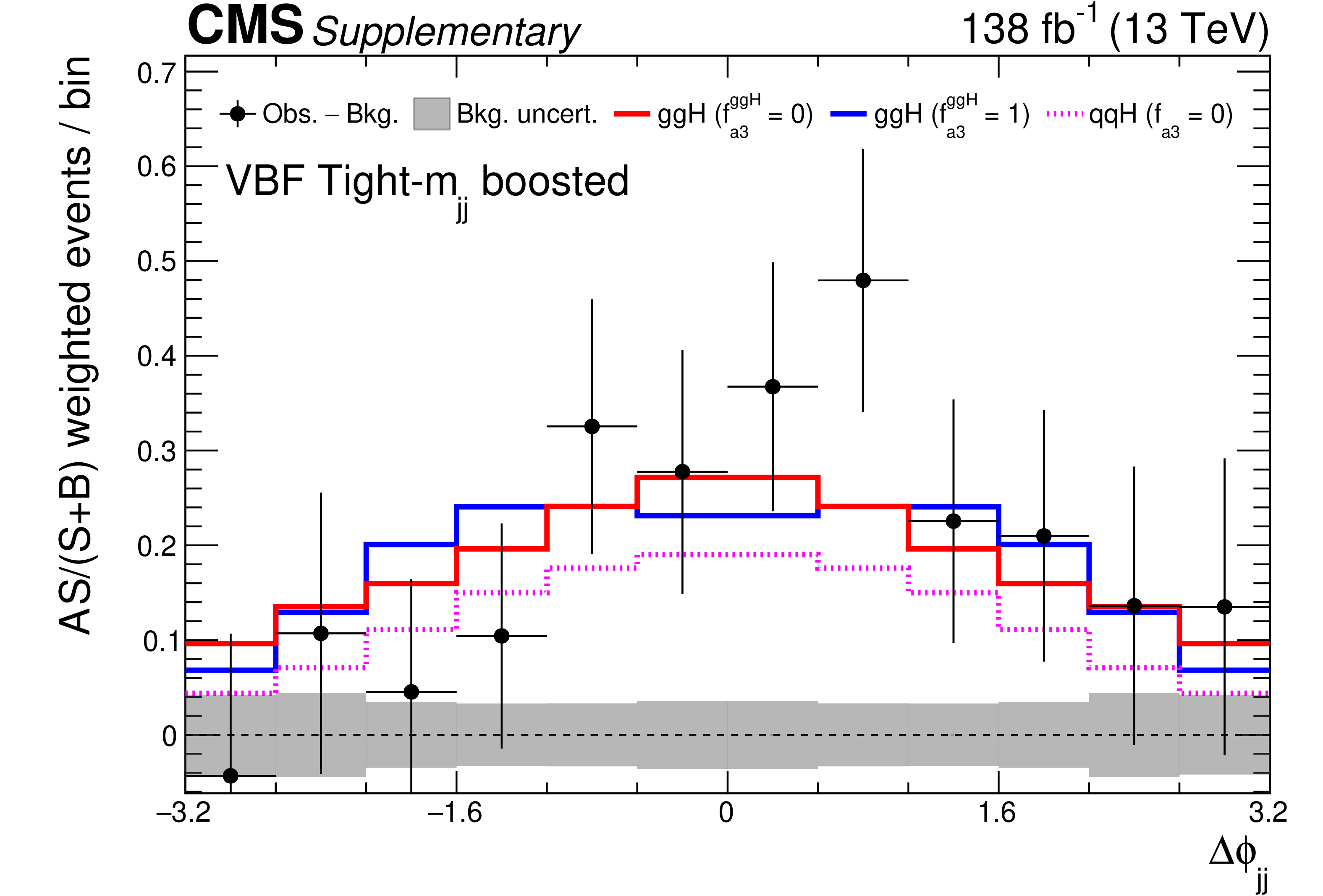
The $\Delta \phi _{\mathrm {jj}}$ distribution for all channels combined. Events were collected from all years and $m_{\tau \tau}$ bins in the VBF high-$m_{\mathrm {jj}}$ boosted category. The non- $\mathrm{H} \rightarrow \tau \tau $ background is subtracted from the data. The events are reweighed by $A\,S/(S+B)$, in which $S$ and $B$ are the ggH signal and background rates, respectively, and $A$ is a measure for the average asymmetry between the scalar ($f_{a3}^{\mathrm{g} \mathrm{g} \mathrm{H}}=$ 0) and pseudoscalar ($f_{a3}^{\mathrm{g} \mathrm{g} \mathrm{H}}=$ 1) distributions. The definition of the value of $A$ per bin is $|N(f_{a3}^{\mathrm{g} \mathrm{g} \mathrm{H}}=0) - N(f_{a3}^{\mathrm{g} \mathrm{g} \mathrm{H}}=1)|/|N(f_{a3}^{\mathrm{g} \mathrm{g} \mathrm{H}}=0) + N(f_{a3}^{\mathrm{g} \mathrm{g} \mathrm{H}}=1)|$ where $N(f_{a3}^{\mathrm{g} \mathrm{g} \mathrm{H}}=0)$ and $N(f_{a3}^{\mathrm{g} \mathrm{g} \mathrm{H}}=1)$ are the expected scalar and pseudoscalar events per bin respectively, and $A$ is normalised to the total number of bins. The scalar ggH distribution is depicted in red, while the pseudoscalar ggH is displayed in blue; both are shown stacked on top of the scalar ($f_{a3}=$ 0) $\mathrm{q} \mathrm{q} \mathrm{H} $ (VBF+$\mathrm{V} \mathrm{H} $) distribution shown by the dashed magenta line. In the predictions, the rate parameters are taken from their best fit values. The grey uncertainty band indicates the uncertainty on the subtracted background component. In total 12 $\Delta \phi _{\mathrm {jj}}$ bins are used with boundaries that range from $-$3.2 to 3.2. Since the physical range of $\Delta \phi _{\mathrm {jj}}$ is between ${\pm} \pi $, the first and last bins actually only include events with 8/3 $ < |\Delta \phi _{\mathrm {jj}}| < \pi $, however, the bin range is extended to $ \pm $3.2 in the plot for visualisation. |
png pdf |
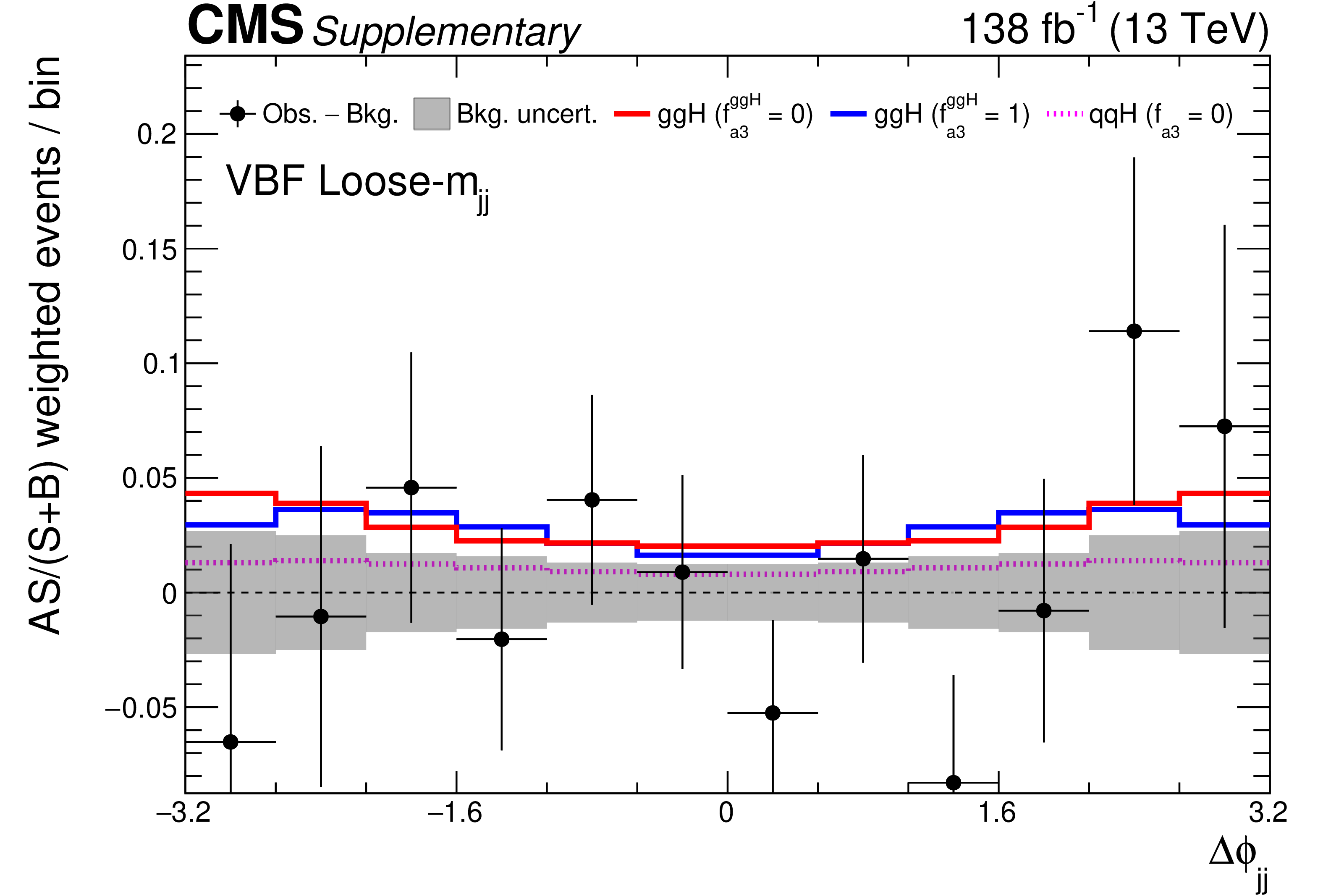
Additional Figure 27:
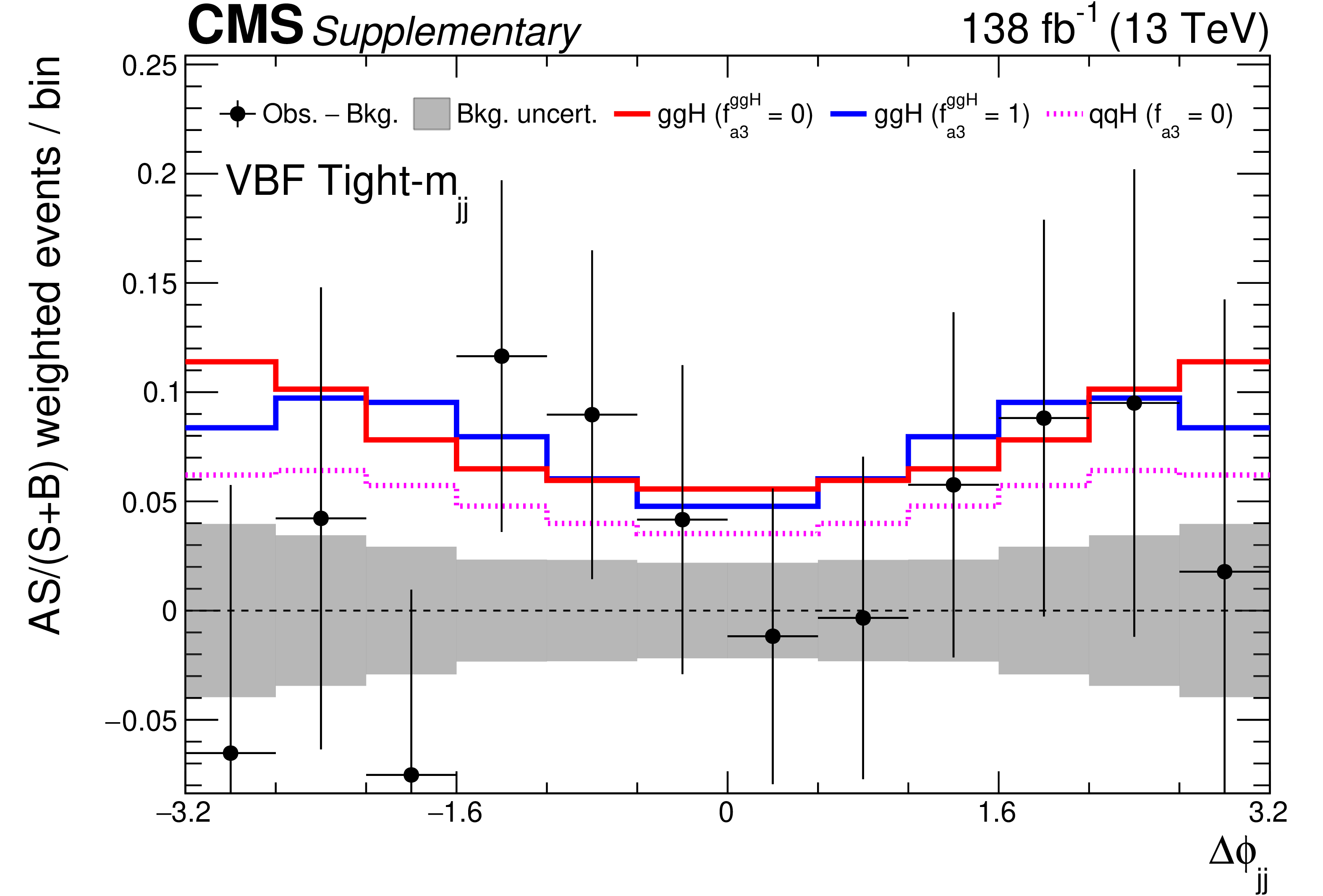
The $\Delta \phi _{\mathrm {jj}}$ distribution for all channels combined. Events were collected from all years and $m_{\tau \tau}$ bins in the VBF high-$m_{\mathrm {jj}}$ category. The non- $\mathrm{H} \rightarrow \tau \tau $ background is subtracted from the data. The events are reweighed by $A\,S/(S+B)$, in which $S$ and $B$ are the ggH signal and background rates, respectively, and $A$ is a measure for the average asymmetry between the scalar ($f_{a3}^{\mathrm{g} \mathrm{g} \mathrm{H}}=$ 0) and pseudoscalar ($f_{a3}^{\mathrm{g} \mathrm{g} \mathrm{H}}=$ 1) distributions. The definition of the value of $A$ per bin is $|N(f_{a3}^{\mathrm{g} \mathrm{g} \mathrm{H}}=0) - N(f_{a3}^{\mathrm{g} \mathrm{g} \mathrm{H}}=1)|/|N(f_{a3}^{\mathrm{g} \mathrm{g} \mathrm{H}}=0) + N(f_{a3}^{\mathrm{g} \mathrm{g} \mathrm{H}}=1)|$ where $N(f_{a3}^{\mathrm{g} \mathrm{g} \mathrm{H}}=0)$ and $N(f_{a3}^{\mathrm{g} \mathrm{g} \mathrm{H}}=1)$ are the expected scalar and pseudoscalar events per bin respectively, and $A$ is normalised to the total number of bins. The scalar ggH distribution is depicted in red, while the pseudoscalar ggH is displayed in blue; both are shown stacked on top of the scalar ($f_{a3}=$ 0) $\mathrm{q} \mathrm{q} \mathrm{H} $ (VBF+$\mathrm{V} \mathrm{H} $) distribution shown by the dashed magenta line. In the predictions, the rate parameters are taken from their best fit values. The grey uncertainty band indicates the uncertainty on the subtracted background component. In total 12 $\Delta \phi _{\mathrm {jj}}$ bins are used with boundaries that range from $-$3.2 to 3.2. Since the physical range of $\Delta \phi _{\mathrm {jj}}$ is between ${\pm} \pi $, the first and last bins actually only include events with 8/3 $ < |\Delta \phi _{\mathrm {jj}}| < \pi $, however, the bin range is extended to $ \pm $3.2 in the plot for visualisation. |
png pdf |
Additional Figure 28:
The $\Delta \phi _{\mathrm {jj}}$ distribution for all channels combined. Events were collected from all years and $m_{\tau \tau}$ bins in the VBF low-$m_{\mathrm {jj}}$ boosted category. The non- $\mathrm{H} \rightarrow \tau \tau $ background is subtracted from the data. The events are reweighed by $A\,S/(S+B)$, in which $S$ and $B$ are the ggH signal and background rates, respectively, and $A$ is a measure for the average asymmetry between the scalar ($f_{a3}^{\mathrm{g} \mathrm{g} \mathrm{H}}=$ 0) and pseudoscalar ($f_{a3}^{\mathrm{g} \mathrm{g} \mathrm{H}}=$ 1) distributions. The definition of the value of $A$ per bin is $|N(f_{a3}^{\mathrm{g} \mathrm{g} \mathrm{H}}=0) - N(f_{a3}^{\mathrm{g} \mathrm{g} \mathrm{H}}=1)|/|N(f_{a3}^{\mathrm{g} \mathrm{g} \mathrm{H}}=0) + N(f_{a3}^{\mathrm{g} \mathrm{g} \mathrm{H}}=1)|$ where $N(f_{a3}^{\mathrm{g} \mathrm{g} \mathrm{H}}=0)$ and $N(f_{a3}^{\mathrm{g} \mathrm{g} \mathrm{H}}=1)$ are the expected scalar and pseudoscalar events per bin respectively, and $A$ is normalised to the total number of bins. The scalar ggH distribution is depicted in red, while the pseudoscalar ggH is displayed in blue; both are shown stacked on top of the scalar ($f_{a3}=$ 0) $\mathrm{q} \mathrm{q} \mathrm{H} $ (VBF+$\mathrm{V} \mathrm{H} $) distribution shown by the dashed magenta line. In the predictions, the rate parameters are taken from their best fit values. The grey uncertainty band indicates the uncertainty on the subtracted background component. In total 12 $\Delta \phi _{\mathrm {jj}}$ bins are used with boundaries that range from $-$3.2 to 3.2. Since the physical range of $\Delta \phi _{\mathrm {jj}}$ is between ${\pm} \pi $, the first and last bins actually only include events with 8/3 $ < |\Delta \phi _{\mathrm {jj}}| < \pi $, however, the bin range is extended to $ \pm $3.2 in the plot for visualisation. |
png pdf |
Additional Figure 29:
The $\Delta \phi _{\mathrm {jj}}$ distribution for all channels combined. Events were collected from all years and $m_{\tau \tau}$ bins in the VBF low-$m_{\mathrm {jj}}$ category. The non- $\mathrm{H} \rightarrow \tau \tau $ background is subtracted from the data. The events are reweighed by $A\,S/(S+B)$, in which $S$ and $B$ are the ggH signal and background rates, respectively, and $A$ is a measure for the average asymmetry between the scalar ($f_{a3}^{\mathrm{g} \mathrm{g} \mathrm{H}}=$ 0) and pseudoscalar ($f_{a3}^{\mathrm{g} \mathrm{g} \mathrm{H}}=$ 1) distributions. The definition of the value of $A$ per bin is $|N(f_{a3}^{\mathrm{g} \mathrm{g} \mathrm{H}}=0) - N(f_{a3}^{\mathrm{g} \mathrm{g} \mathrm{H}}=1)|/|N(f_{a3}^{\mathrm{g} \mathrm{g} \mathrm{H}}=0) + N(f_{a3}^{\mathrm{g} \mathrm{g} \mathrm{H}}=1)|$ where $N(f_{a3}^{\mathrm{g} \mathrm{g} \mathrm{H}}=0)$ and $N(f_{a3}^{\mathrm{g} \mathrm{g} \mathrm{H}}=1)$ are the expected scalar and pseudoscalar events per bin respectively, and $A$ is normalised to the total number of bins. The scalar ggH distribution is depicted in red, while the pseudoscalar ggH is displayed in blue; both are shown stacked on top of the scalar ($f_{a3}=$ 0) $\mathrm{q} \mathrm{q} \mathrm{H} $ (VBF+$\mathrm{V} \mathrm{H} $) distribution shown by the dashed magenta line. In the predictions, the rate parameters are taken from their best fit values. The grey uncertainty band indicates the uncertainty on the subtracted background component. In total 12 $\Delta \phi _{\mathrm {jj}}$ bins are used with boundaries that range from $-$3.2 to 3.2. Since the physical range of $\Delta \phi _{\mathrm {jj}}$ is between ${\pm} \pi $, the first and last bins actually only include events with 8/3 $ < |\Delta \phi _{\mathrm {jj}}| < \pi $, however, the bin range is extended to $ \pm $3.2 in the plot for visualisation. |

png pdf |
Additional Figure 30:
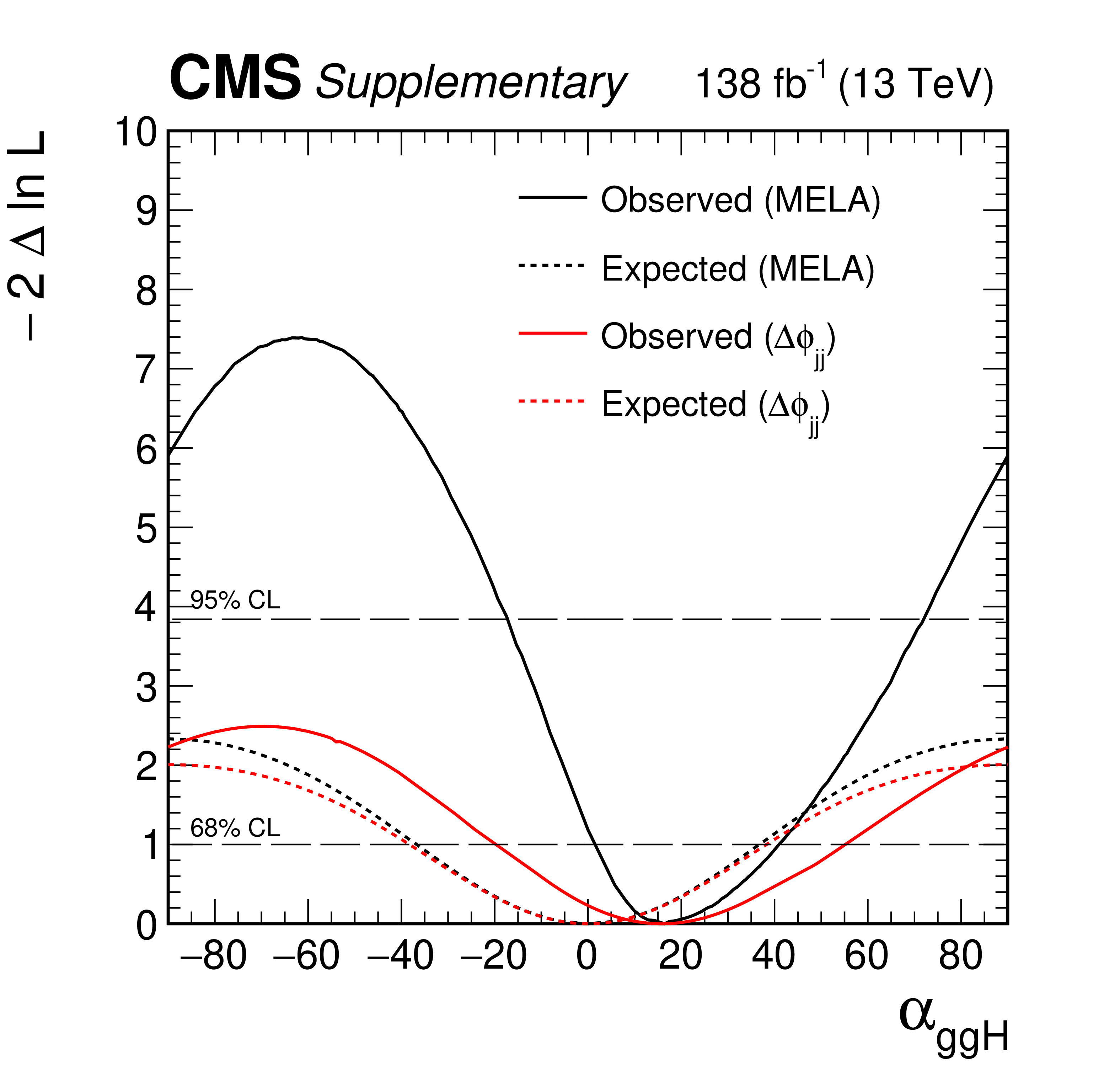
Observed (solid) and expected (dashed) likelihood scans of $\alpha _{\mathrm{g} \mathrm{g} \mathrm{H}}$ obtained with the MELA method. The $\alpha _{\mathrm{g} \mathrm{g} \mathrm{H}}$ parameter is defined as $\alpha _{\mathrm{g} \mathrm{g} \mathrm{H}}=\arctan(a_{3}^{\mathrm{g} \mathrm{g}}/a_{2}^{\mathrm{g} \mathrm{g}})$. |
png pdf |
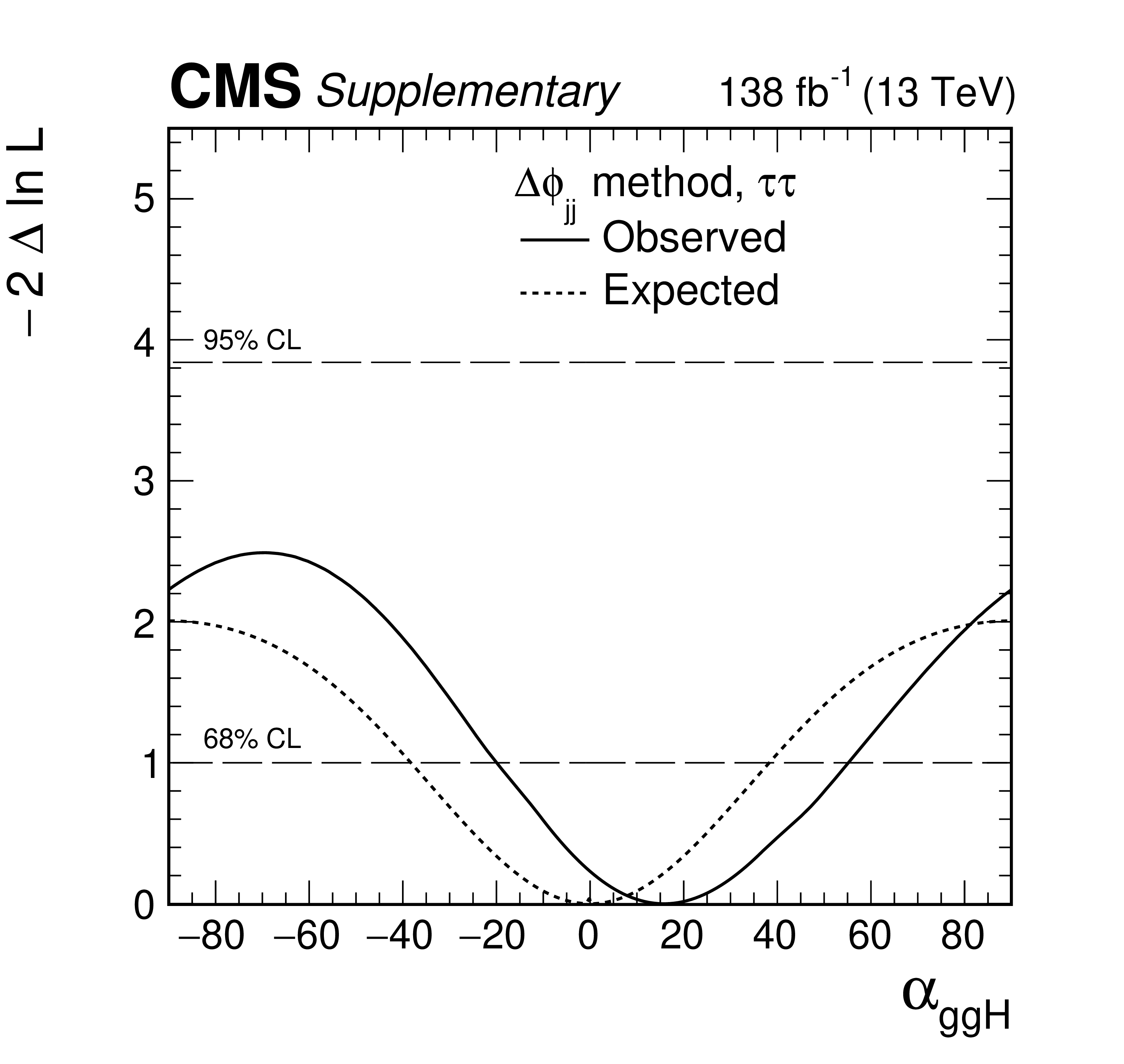
Additional Figure 31:
Observed (solid) and expected (dashed) likelihood scans of $\alpha _{\mathrm{g} \mathrm{g} \mathrm{H}}$ obtained with the $\Delta \phi _{\mathrm {jj}}$ method. The $\alpha _{\mathrm{g} \mathrm{g} \mathrm{H}}$ parameter is defined as $\alpha _{\mathrm{g} \mathrm{g} \mathrm{H}}=\arctan(a_{3}^{\mathrm{g} \mathrm{g}}/a_{2}^{\mathrm{g} \mathrm{g}})$. |

png pdf |
Additional Figure 32:
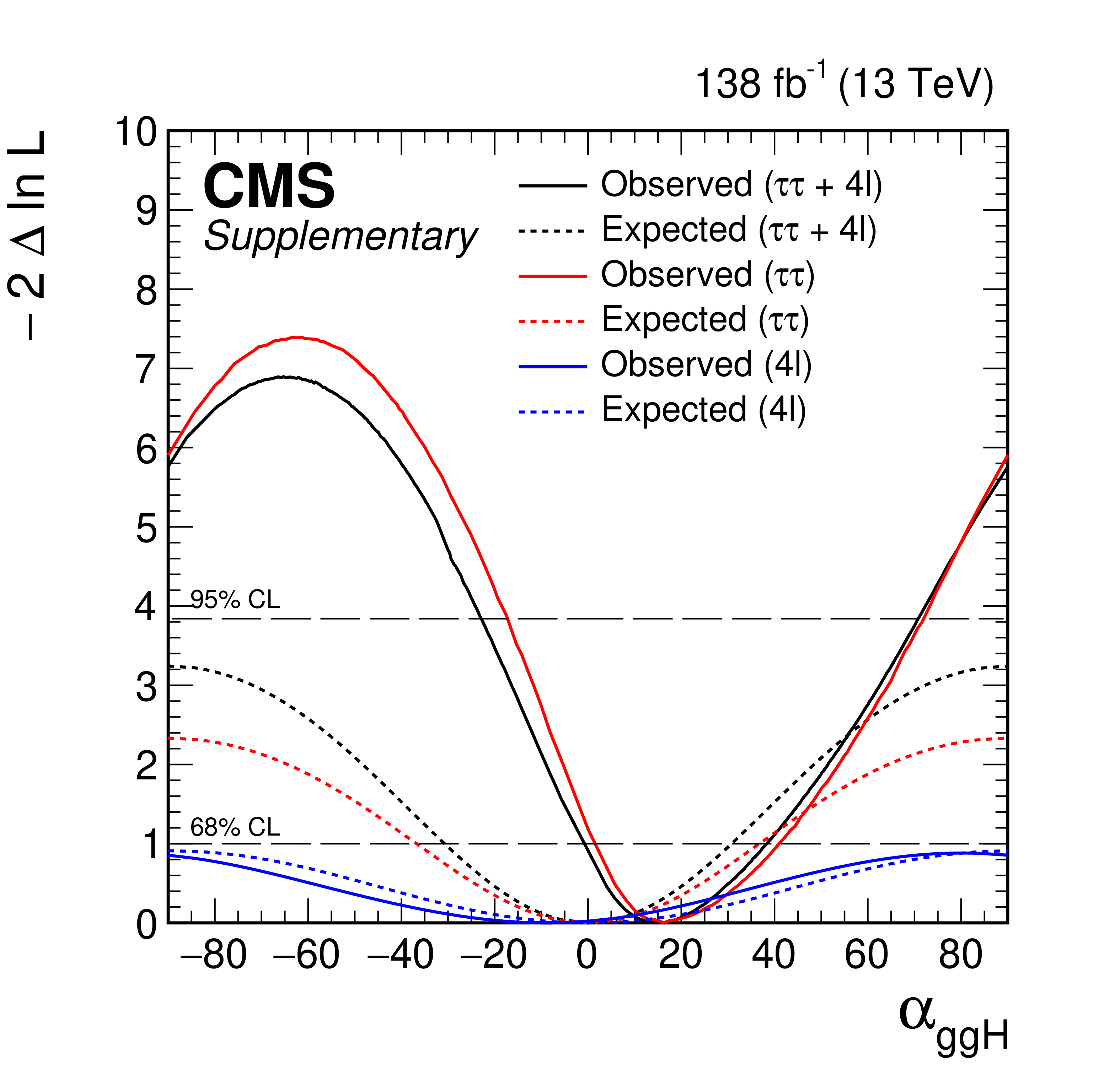
Observed (solid) and expected (dashed) likelihood scans of $\alpha _{\mathrm{g} \mathrm{g} \mathrm{H}}$ obtained with the combination of results using the $\mathrm{H} \to \tau \tau $ (obtained with the MELA method) and $\mathrm{H} \to 4\ell $ decay channels. |
png pdf |
Additional Figure 33:
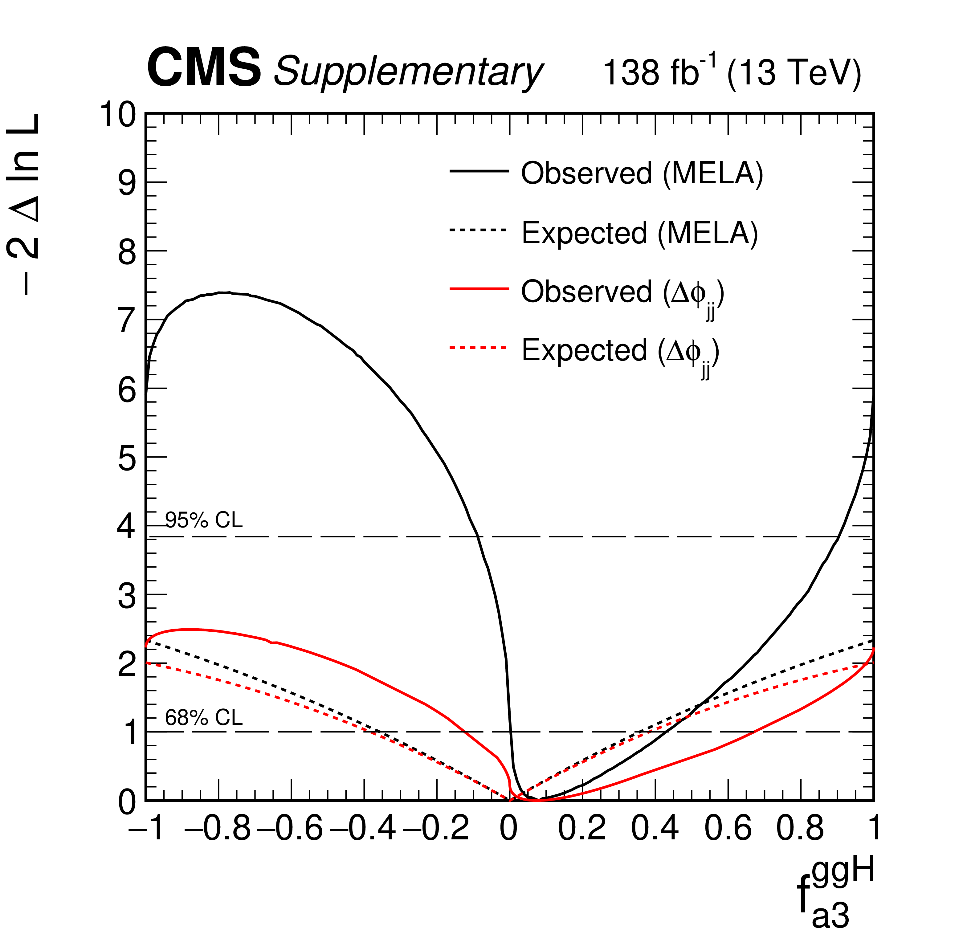
Observed (solid) and expected (dashed) likelihood scans of $f_{a3}^{\mathrm{g} \mathrm{g} \mathrm{H}}$ obtained with the MELA (black) and $\Delta \phi _{\mathrm {jj}}$ (red) methods. |
png pdf |
Additional Figure 34:
Observed (solid) and expected (dashed) likelihood scans of $\alpha ^{\mathrm{H} \mathrm {ff}}$ obtained with the MELA (black) and $\Delta \phi _{\mathrm {jj}}$ (red) methods. |
png pdf |
Additional Figure 35:
Observed (solid) and expected (dashed) likelihood scans of $\alpha _{\mathrm{g} \mathrm{g} \mathrm{H}}$ obtained with the MELA (black) and $\Delta \phi _{\mathrm {jj}}$ (red) methods. The $\alpha _{\mathrm{g} \mathrm{g} \mathrm{H}}$ parameter is defined as $\alpha _{\mathrm{g} \mathrm{g} \mathrm{H}}=\arctan(a_{3}^{\mathrm{g} \mathrm{g}}/a_{2}^{\mathrm{g} \mathrm{g}})$. |
png pdf |
Additional Figure 36:
Observed (solid) and expected (dashed) likelihood scans of $f_{a3}^{\mathrm{g} \mathrm{g} \mathrm{H}}$ obtained with the combination of results using the $\mathrm{H} \to \tau \tau $ (obtained with the MELA method) and $\mathrm{H} \to 4\ell $ decay channels. |

png pdf |
Additional Figure 37:
Observed (solid) and expected (dashed) likelihood scans of $\alpha ^{\mathrm{H} \mathrm {ff}}$ obtained with the combination of results using the $\mathrm{H} \to \tau \tau $ (obtained with the MELA method) and $\mathrm{H} \to 4\ell $ decay channels. |
png pdf |
Additional Figure 38:
Observed (solid) and expected (dashed) likelihood scans of $\alpha _{\mathrm{g} \mathrm{g} \mathrm{H}}$ obtained with the combination of results using the $\mathrm{H} \to \tau \tau $ (obtained with the MELA method) and $\mathrm{H} \to 4\ell $ decay channels. |
png pdf |
Additional Figure 39:
Observed (solid) and expected (dashed) likelihood scans of $f_{\textit {CP}}^{\mathrm{H} \mathrm{t} \mathrm{t}}$ obtained with the combination of results using the $\mathrm{H} \to \tau \tau $ (obtained with the MELA method), $\mathrm{H} \to 4\ell $, and $\mathrm{H} \to \gamma \gamma $ decay channels. |
png pdf |
Additional Figure 40:
Observed (solid) and expected (dashed) likelihood scans of $f_{a3}$ in Approach 1 obtained with the combination of results using the $\mathrm{H} \to \tau \tau $ and $\mathrm{H} \to 4\ell $ decay channels. |
png pdf |
Additional Figure 41:
Observed (solid) and expected (dashed) likelihood scans of $f_{a2}$ in Approach 1 obtained with the combination of results using the $\mathrm{H} \to \tau \tau $ and $\mathrm{H} \to 4\ell $ decay channels. |
png pdf |
Additional Figure 42:
Observed (solid) and expected (dashed) likelihood scans of $f_{\Lambda 1}$ in Approach 1 obtained with the combination of results using the $\mathrm{H} \to \tau \tau $ and $\mathrm{H} \to 4\ell $ decay channels. |
png pdf |
Additional Figure 43:
Observed (solid) and expected (dashed) likelihood scans of $f_{\Lambda 1}^{\mathrm{Z} \gamma}$ in Approach 1 obtained with the combination of results using the $\mathrm{H} \to \tau \tau $ and $\mathrm{H} \to 4\ell $ decay channels. |
png pdf |
Additional Figure 44:
Observed (solid) and expected (dashed) likelihood scans of $f_{a3}$ in Approach 2 obtained with the combination of results using the $\mathrm{H} \to \tau \tau $ and $\mathrm{H} \to 4\ell $ decay channels. |
png pdf |
Additional Figure 45:
Observed (solid) and expected (dashed) likelihood scans of $f_{a3}$ in Approach 1 obtained with the combination of results using the $\mathrm{H} \to \tau \tau $ and $\mathrm{H} \to 4\ell $ decay channels. |
png pdf |
Additional Figure 46:
Observed (solid) and expected (dashed) likelihood scans of $f_{a2}$ in Approach 1 obtained with the combination of results using the $\mathrm{H} \to \tau \tau $ and $\mathrm{H} \to 4\ell $ decay channels. |
png pdf |
Additional Figure 47:
Observed (solid) and expected (dashed) likelihood scans of $f_{\Lambda 1}$ in Approach 1 obtained with the combination of results using the $\mathrm{H} \to \tau \tau $ and $\mathrm{H} \to 4\ell $ decay channels. |

png pdf |
Additional Figure 48:
Observed (solid) and expected (dashed) likelihood scans of $f_{\Lambda 1}^{\mathrm{Z} \gamma}$ in Approach 1 obtained with the combination of results using the $\mathrm{H} \to \tau \tau $ and $\mathrm{H} \to 4\ell $ decay channels. |
png pdf |
Additional Figure 49:
Observed (solid) and expected (dashed) likelihood scans of $f_{a3}$ in Approach 2 obtained with the combination of results using the $\mathrm{H} \to \tau \tau $ and $\mathrm{H} \to 4\ell $ decay channels. |

png pdf |
Additional Figure 50:
A candidate ggH + 2 jet event in the $\mu {\tau _\mathrm {h}} $ final state, as seen in the $\rho $-$\phi $ plane. The $\mu $ candidate is shown in red, and the missing transverse momentum vector is indicated by the purple arrow. Three jets are visible as shown in yellow and cyan. The $ {\tau _\mathrm {h}} $ candidate corresponds to the cyan colored jet. The two other jets have a CP-even-like topology ($ {| \Delta \phi _{\mathrm {jj}} |}\approx \pi $). The dijet pair have $\Delta \phi _{\mathrm {jj}}=0.94\pi $, $ {| \Delta \eta _{jj} |}=3.23$, and $m_{\mathrm {jj}} = $ 510 GeV. The event was recorded during the 2018 data-taking period (event number, run, luminosity section = 366863438, 322356, 194). |
png pdf |
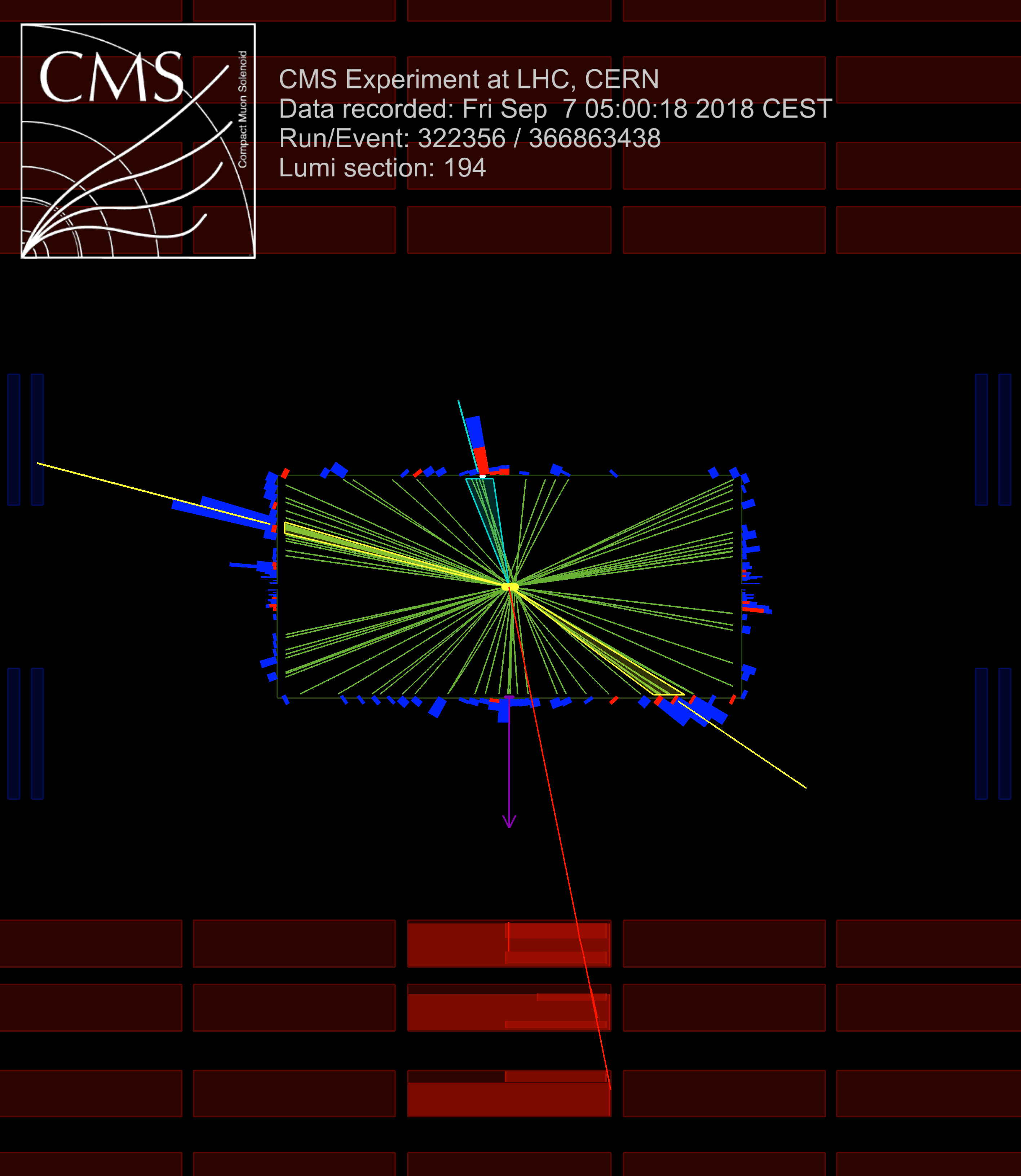
Additional Figure 51:
A candidate ggH + 2 jet event in the $\mu {\tau _\mathrm {h}} $ final state, as seen in the $\rho $-$z$ plane. The $\mu $ candidate is shown in red, and the missing transverse momentum vector is indicated by the purple arrow. Three jets are visible as shown in yellow and cyan. The $ {\tau _\mathrm {h}} $ candidate corresponds to the cyan colored jet. The two other jets have a CP-even-like topology ($ {| \Delta \phi _{\mathrm {jj}} |}\approx \pi $). The dijet pair have $\Delta \phi _{\mathrm {jj}}=0.94\pi $, $ {| \Delta \eta _{jj} |}=3.23$, and $m_{\mathrm {jj}} = $ 510 GeV. The event was recorded during the 2018 data-taking period (event number, run, luminosity section = 366863438, 322356, 194). |
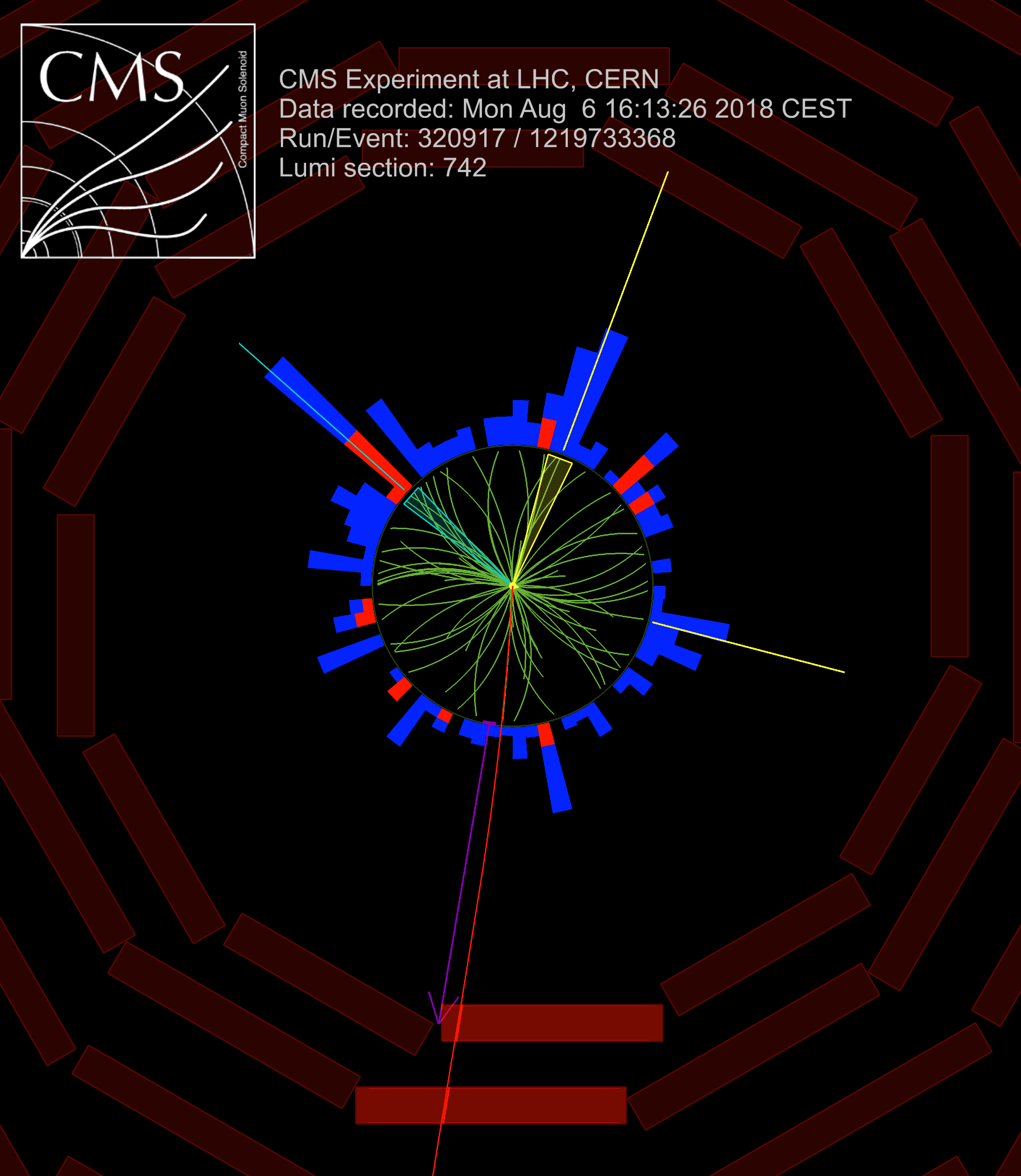
png pdf |
Additional Figure 52:
A candidate ggH + 2 jet event in the $\mu {\tau _\mathrm {h}} $ final state, as seen in the $\rho $-$\phi $ plane. The $\mu $ candidate is shown in red, and the missing transverse momentum vector is indicated by the purple arrow. Three jets are visible as shown in yellow and cyan. The $ {\tau _\mathrm {h}} $ candidate corresponds to the cyan colored jet. The two other jets have a CP-odd-like topology ($ {| \Delta \phi _{\mathrm {jj}} |}\approx \frac {\pi}{2}$). The dijet pair have $\Delta \phi _{\mathrm {jj}}=$ $-$0.47$\pi $, $ {| \Delta \eta _{jj} |}=$ 5.24, and $m_{\mathrm {jj}} = $ 582 GeV. The event was recorded during the 2018 data-taking period (event number, run, luminosity section = 1219733368, 320917, 742). |

png pdf |
Additional Figure 53:
A candidate ggH + 2 jet event in the $\mu {\tau _\mathrm {h}} $ final state, as seen in the $\rho $-$z$ plane. The $\mu $ candidate is shown in red, and the missing transverse momentum vector is indicated by the purple arrow. Three jets are visible as shown in yellow and cyan. The $ {\tau _\mathrm {h}} $ candidate corresponds to the cyan colored jet. The two other jets have a CP-odd-like topology ($ {| \Delta \phi _{\mathrm {jj}} |}\approx \frac {\pi}{2}$). The dijet pair have $\Delta \phi _{\mathrm {jj}}= $ $-$0.47$\pi $, $ {| \Delta \eta _{jj} |}=$ 5.24, and $m_{\mathrm {jj}} = $ 582 GeV. The event was recorded during the 2018 data-taking period (event number, run, luminosity section = 1219733368, 320917, 742). |
png pdf |
Additional Figure 54:
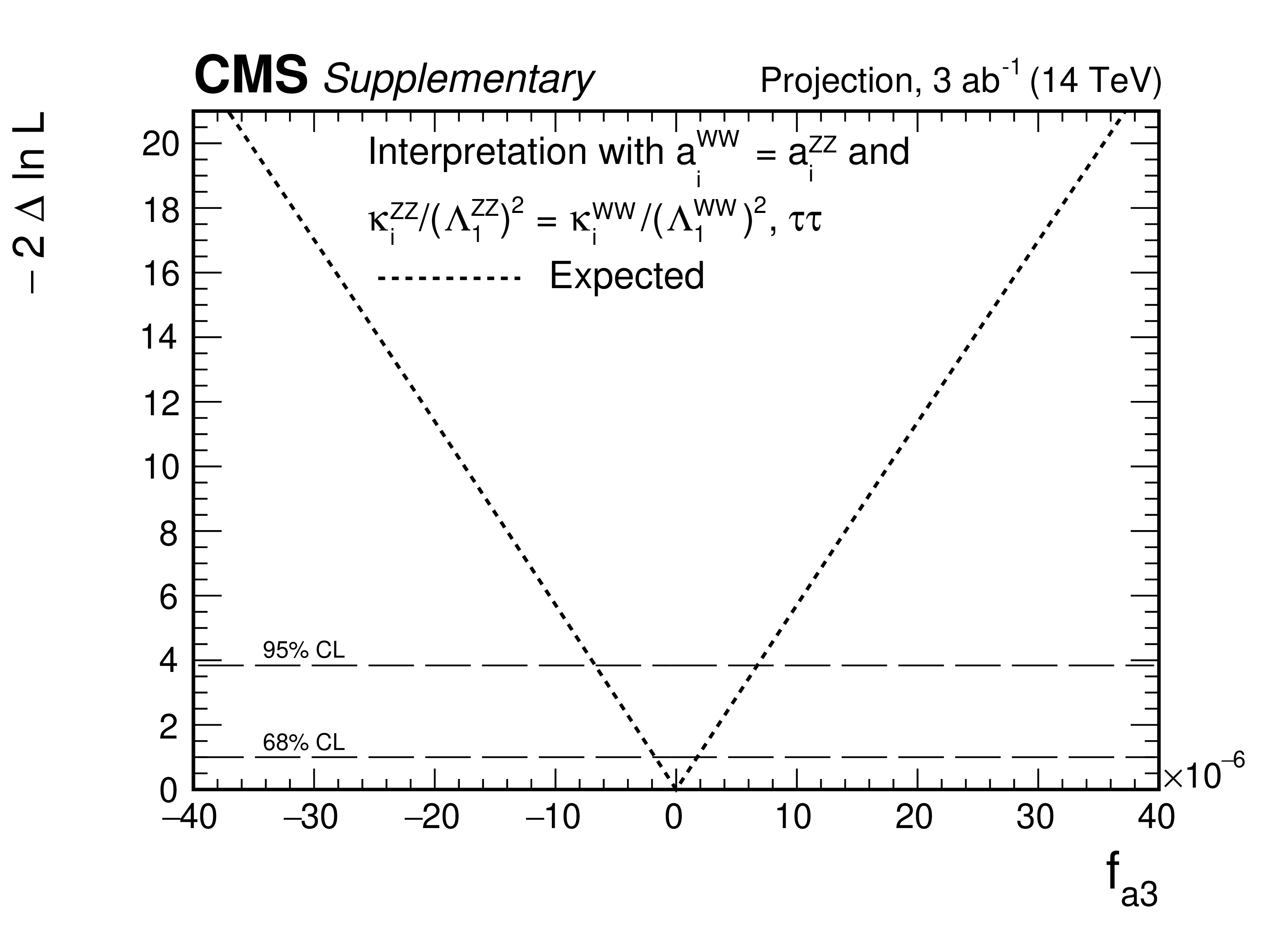
Projection of the expected likelihood scan of $f_{a3}$ based on the Run 2 analysis to an integrated luminosity of 3 ab$^{-1}$ at $\sqrt {s} = $ 14 TeV. "Bin-by-bin" systematic uncertainties are ignored in the extrapolation. The other systematic uncertainties are adjusted to the scheme used for the YR18 HL-LHC projections (arXiv:1902.00134). The relationship between the $a_i^{\mathrm{W} \mathrm{W}}$ and $a_i^{\mathrm{Z} \mathrm{Z}}$ couplings is assumed to satisfy ${a_i^{\mathrm{W} \mathrm{W}}=a_i^{\mathrm{Z} \mathrm{Z}}}$ and ${\kappa _i^{\mathrm{Z} \mathrm{Z}}/(\Lambda _{1}^{\mathrm{Z} \mathrm{Z}})^2}$ = ${\kappa _i^{\mathrm{W} \mathrm{W}}/(\Lambda _{1}^{\mathrm{W} \mathrm{W}})^2}$ (Approach 1). |
png pdf |
Additional Figure 55:
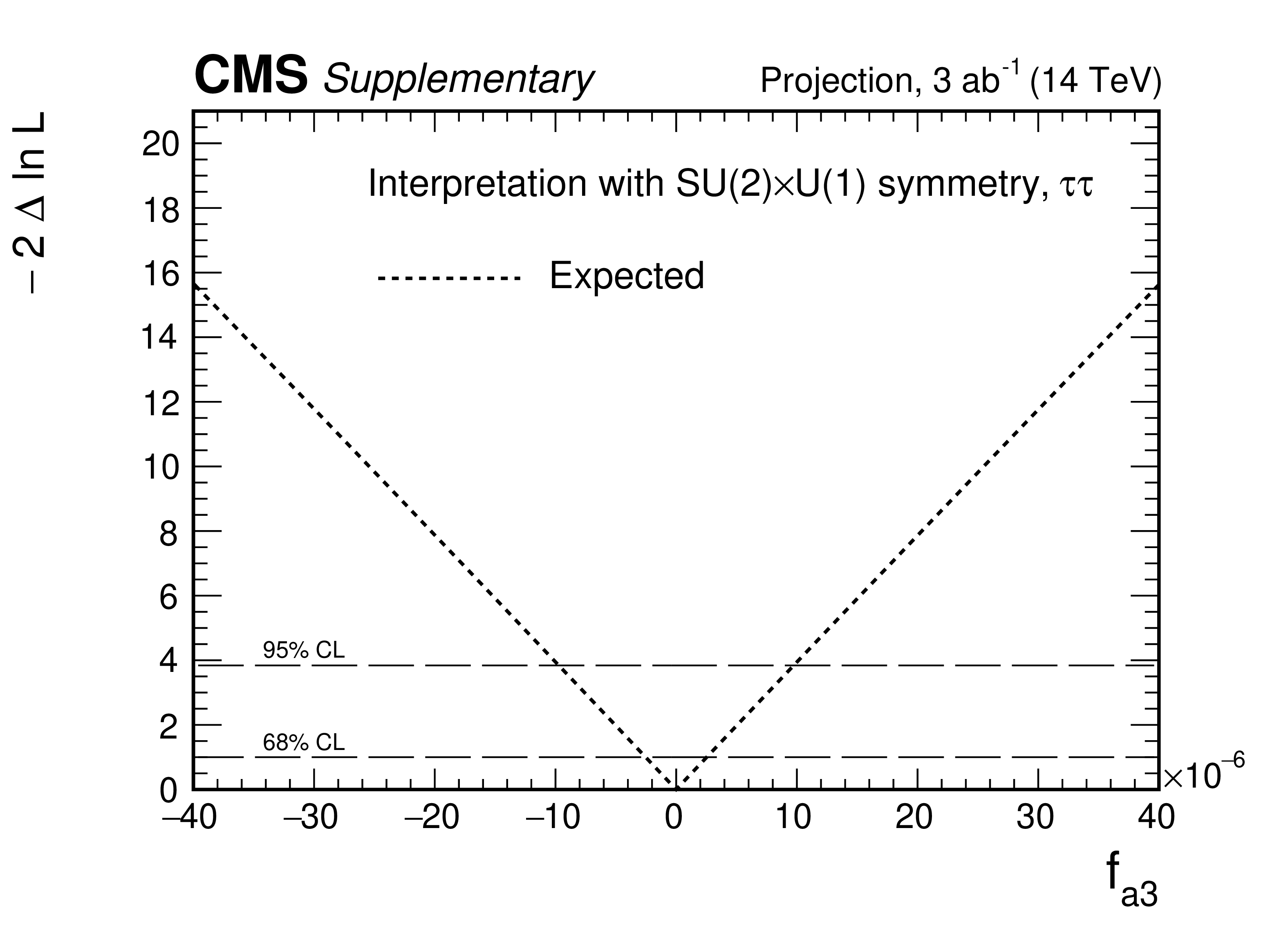
Projection of the expected likelihood scan of $f_{a3}$ based on the Run 2 analysis to an integrated luminosity of 3 ab$^{-1}$ at $\sqrt {s} = $ 14 TeV. "Bin-by-bin" systematic uncertainties are ignored in the extrapolation. The other systematic uncertainties are adjusted to the scheme used for the YR18 HL-LHC projections (arXiv:1902.00134). The expected likelihood scan of $f_{a3}$ is reinterpretetd with custodial and SU(2)$\times $U(1) symmetries in the relationships of anomalous couplings (Approach 2). |

png pdf |
Additional Figure 56:
Projection of the expected likelihood scan of $f_{a3}^{\mathrm{g} \mathrm{g} \mathrm{H}}$ based on the Run 2 analysis to an integrated luminosity of 3 ab$^{-1}$ at $\sqrt {s} = $ 14 TeV. "Bin-by-bin" systematic uncertainties are ignored in the extrapolation. The other systematic uncertainties are adjusted to the scheme used for the YR18 HL-LHC projections (arXiv:1902.00134). The extrapolation is performed on the result obtained with the MELA method. |
| Additional Tables | |
png pdf |
Additional Table 1:
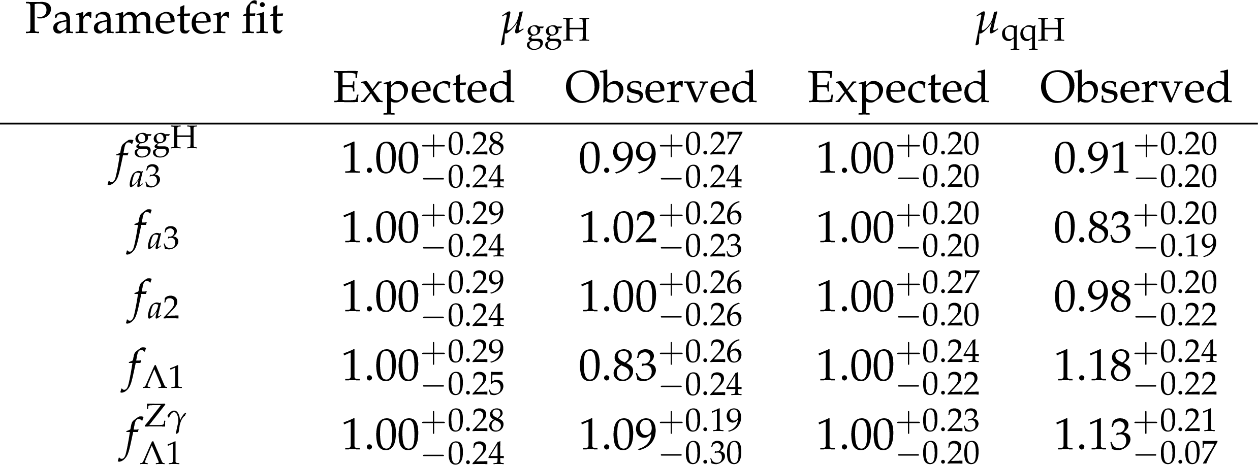
The expected and observed values of the signal strength modifiers that scale the ggH ($\mu _{\mathrm{g} \mathrm{g} \mathrm{H}}$) and VBF+$\mathrm{V} \mathrm{H} $ ($\mu _{\mathrm{q} \mathrm{q} \mathrm{H}}$) signals in the $\mathrm{H} \to \tau \tau $ final state. The best fit values are shown for each of the fits used to extract a given anomalous coupling parameter. |
png pdf |
Additional Table 2:
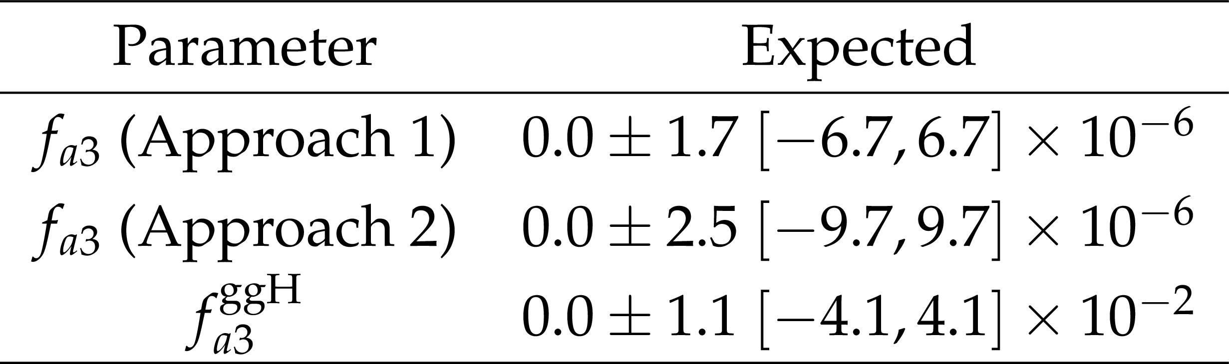
Projections of allowed 68% (central values with uncertainties) and 95% CL (in square brackets) intervals on $f_{a3}$ and $f_{a3}^{\gamma\gamma\mathrm{H}}$ based on the Run 2 analysis to an integrated luminosity of 3 ab$^{-1}$ at $\sqrt{s}=$ 14 TeV. "Bin-by-bin" systematic uncertainties are ignored in the extrapolation. The other systematic uncertainties are adjusted to the scheme used for the YR18 HL-LHC projections (arXiv:1902.00134). Two different approaches are adopted for $f_{a3}$ scans to set the relationship between the $a_i^{\mathrm{W}\mathrm{W}}$ and $a_i^{\mathrm{Z}\mathrm{Z}}$ couplings: assuming ${a_i^{\mathrm{W}\mathrm{W}}=a_i^{\mathrm{Z}\mathrm{Z}}}$ and ${\kappa_i^{\mathrm{Z}\mathrm{Z}}/(\Lambda_{1}^{\mathrm{Z}\mathrm{Z}})^2}$ = ${\kappa_i^{\mathrm{W}\mathrm{W}}/(\Lambda_{1}^{\mathrm{W}\mathrm{W}})^2}$ (Approach 1) or considering custodial and SU(2)$\times$U(1) symmetries in the relationships of anomalous couplings (Approach 2). |
| References | ||||
| 1 | ATLAS Collaboration | Observation of a new particle in the search for the standard model Higgs boson with the ATLAS detector at the LHC | PLB 716 (2012) 1 | 1207.7214 |
| 2 | CMS Collaboration | Observation of a new boson at a mass of 125 GeV with the CMS experiment at the LHC | PLB 716 (2012) 30 | CMS-HIG-12-028 1207.7235 |
| 3 | CMS Collaboration | Observation of a new boson with mass near 125 GeV in pp collisions at $ \sqrt{s} = $ 7 and 8 TeV | JHEP 06 (2013) 081 | CMS-HIG-12-036 1303.4571 |
| 4 | S. L. Glashow | Partial-symmetries of weak interactions | NP 22 (1961) 579 | |
| 5 | F. Englert and R. Brout | Broken symmetry and the mass of gauge vector mesons | PRL 13 (1964) 321 | |
| 6 | P. W. Higgs | Broken symmetries, massless particles and gauge fields | PL12 (1964) 132 | |
| 7 | P. W. Higgs | Broken symmetries and the masses of gauge bosons | PRL 13 (1964) 508 | |
| 8 | G. S. Guralnik, C. R. Hagen, and T. W. B. Kibble | Global conservation laws and massless particles | PRL 13 (1964) 585 | |
| 9 | S. Weinberg | A model of leptons | PRL 19 (1967) 1264 | |
| 10 | A. Salam | Weak and electromagnetic interactions | Conf. Proc. C 680519 (1968) 367 | |
| 11 | CMS Collaboration | Constraints on the spin-parity and anomalous HVV couplings of the Higgs boson in proton collisions at 7 and 8 TeV | PRD 92 (2015) 012004 | CMS-HIG-14-018 1411.3441 |
| 12 | ATLAS Collaboration | Study of the spin and parity of the Higgs boson in diboson decays with the ATLAS detector | EPJC 75 (2015) 476 | 1506.05669 |
| 13 | CMS Collaboration | Study of the mass and spin-parity of the Higgs boson candidate via its decays to Z boson pairs | PRL 110 (2013) 081803 | CMS-HIG-12-041 1212.6639 |
| 14 | CMS Collaboration | Measurement of the properties of a Higgs boson in the four-lepton final state | PRD 89 (2014) 092007 | CMS-HIG-13-002 1312.5353 |
| 15 | CMS Collaboration | Limits on the Higgs boson lifetime and width from its decay to four charged leptons | PRD 92 (2015) 072010 | CMS-HIG-14-036 1507.06656 |
| 16 | CMS Collaboration | Combined search for anomalous pseudoscalar HVV couplings in VH(H $ \to \text{b}\bar{\text{b}} $) production and H $ \to $ VV decay | PLB 759 (2016) 672 | CMS-HIG-14-035 1602.04305 |
| 17 | CMS Collaboration | Constraints on anomalous Higgs boson couplings using production and decay information in the four-lepton final state | PLB 775 (2017) 1 | CMS-HIG-17-011 1707.00541 |
| 18 | CMS Collaboration | Measurements of the Higgs boson width and anomalous HVV couplings from on-shell and off-shell production in the four-lepton final state | PRD 99 (2019) 112003 | CMS-HIG-18-002 1901.00174 |
| 19 | CMS Collaboration | Constraints on anomalous HVV couplings from the production of Higgs bosons decaying to $ \tau $ lepton pairs | PRD 100 (2019) 112002 | CMS-HIG-17-034 1903.06973 |
| 20 | CMS Collaboration | Measurements of $ \text{t}\bar{\text{t}}\mathrm{H} $ production and the CP structure of the Yukawa interaction between the Higgs boson and top quark in the diphoton decay channel | PRL 125 (2020) 061801 | CMS-HIG-19-013 2003.10866 |
| 21 | CMS Collaboration | Constraints on anomalous Higgs boson couplings to vector bosons and fermions in its production and decay using the four-lepton final state | PRD 104 (2021) 052004 | CMS-HIG-19-009 2104.12152 |
| 22 | CMS Collaboration | Analysis of the $ CP $ structure of the Yukawa coupling between the Higgs boson and $ \tau $ leptons in proton-proton collisions at $ \sqrt{s} = $ 13 TeV | Submitted to JHEP | CMS-HIG-20-006 2110.04836 |
| 23 | CMS Collaboration | First evidence for off-shell production of the Higgs boson and measurement of its width | Submitted to Nature Physics | CMS-HIG-21-013 2202.06923 |
| 24 | ATLAS Collaboration | Evidence for the spin-0 nature of the Higgs boson using ATLAS data | PLB 726 (2013) 120 | 1307.1432 |
| 25 | ATLAS Collaboration | Test of CP invariance in vector-boson fusion production of the Higgs boson using the optimal observable method in the ditau decay channel with the ATLAS detector | EPJC 76 (2016) 658 | 1602.04516 |
| 26 | ATLAS Collaboration | Measurement of inclusive and differential cross sections in the $ H \rightarrow ZZ^* \rightarrow 4\ell $ decay channel in pp collisions at $ \sqrt{s}= $ 13 TeV with the ATLAS detector | JHEP 10 (2017) 132 | 1708.02810 |
| 27 | ATLAS Collaboration | Measurement of the Higgs boson coupling properties in the $ H\rightarrow ZZ^{*} \rightarrow 4\ell $ decay channel at $ \sqrt{s} = $ 13 TeV with the ATLAS detector | JHEP 03 (2018) 095 | 1712.02304 |
| 28 | ATLAS Collaboration | Measurements of Higgs boson properties in the diphoton decay channel with 36 fb$ ^{-1} $ of pp collision data at $ \sqrt{s} = $ 13 TeV with the ATLAS detector | PRD 98 (2018) 052005 | 1802.04146 |
| 29 | ATLAS Collaboration | Test of CP invariance in vector-boson fusion production of the Higgs boson in the $ H\rightarrow\tau\tau $ channel in proton$ - $proton collisions at $ \sqrt{s} = $ 13 TeV with the ATLAS detector | PLB 805 (2020) 135426 | 2002.05315 |
| 30 | ATLAS Collaboration | CP properties of Higgs boson interactions with top quarks in the $ t\bar{t}H $ and $ tH $ processes using $ H \rightarrow \gamma\gamma $ with the ATLAS detector | PRL 125 (2020) 061802 | 2004.04545 |
| 31 | ATLAS Collaboration | Constraints on Higgs boson properties using $ \mathrm{W}\mathrm{W}^{*}(\rightarrow \mathrm{e}\nu\mu\nu) jj $ production in 36.1 fb$ ^{-1} $ of $ \sqrt{s} = $ 13 TeV pp collisions with the ATLAS detector | Submitted to EPJC | 2109.13808 |
| 32 | Y. Gao et al. | Spin determination of single-produced resonances at hadron colliders | PRD 81 (2010) 075022 | 1001.3396 |
| 33 | S. Bolognesi et al. | Spin and parity of a single-produced resonance at the LHC | PRD 86 (2012) 095031 | 1208.4018 |
| 34 | I. Anderson et al. | Constraining anomalous HVV interactions at proton and lepton colliders | PRD 89 (2014) 035007 | 1309.4819 |
| 35 | A. V. Gritsan, R. Rontsch, M. Schulze, and M. Xiao | Constraining anomalous Higgs boson couplings to the heavy flavor fermions using matrix element techniques | PRD 94 (2016) 055023 | 1606.03107 |
| 36 | CMS Collaboration | HEPData record for this analysis | link | |
| 37 | T. Plehn, D. L. Rainwater, and D. Zeppenfeld | Determining the structure of Higgs couplings at the LHC | PRL 88 (2002) 051801 | hep-ph/0105325 |
| 38 | V. Hankele, G. Klamke, D. Zeppenfeld, and T. Figy | Anomalous Higgs boson couplings in vector boson fusion at the CERN LHC | PRD 74 (2006) 095001 | hep-ph/0609075 |
| 39 | E. Accomando et al. | Workshop on CP studies and non-standard Higgs physics | hep-ph/0608079 | |
| 40 | K. Hagiwara, Q. Li, and K. Mawatari | Jet angular correlation in vector-boson fusion processes at hadron colliders | JHEP 07 (2009) 101 | 0905.4314 |
| 41 | A. De R\' ujula et al. | Higgs look-alikes at the LHC | PRD 82 (2010) 013003 | 1001.5300 |
| 42 | J. Ellis, D. S. Hwang, V. Sanz, and T. You | A fast track towards the `Higgs' spin and parity | JHEP 11 (2012) 134 | 1208.6002 |
| 43 | P. Artoisenet et al. | A framework for Higgs characterisation | JHEP 11 (2013) 043 | 1306.6464 |
| 44 | M. J. Dolan, P. Harris, M. Jankowiak, and M. Spannowsky | Constraining CP-violating Higgs sectors at the LHC using gluon fusion | PRD 90 (2014) 073008 | 1406.3322 |
| 45 | A. Greljo, G. Isidori, J. M. Lindert, and D. Marzocca | Pseudo-observables in electroweak Higgs production | EPJC 76 (2016) 158 | 1512.06135 |
| 46 | J. Davis et al. | Constraining anomalous Higgs boson couplings to virtual photons | 2109.13363 | |
| 47 | A. V. Gritsan et al. | New features in the JHU generator framework: constraining Higgs boson properties from on-shell and off-shell production | PRD 102 (2020) 056022 | 2002.09888 |
| 48 | LHC Higgs Cross Section Working Group | Handbook of LHC Higgs cross sections: 4. deciphering the nature of the Higgs sector | CERN (2016) | 1610.07922 |
| 49 | K. Hamilton, P. Nason, and G. Zanderighi | Finite quark-mass effects in the NNLOPS POWHEG+MiNLO Higgs generator | JHEP 05 (2015) 140 | 1501.04637 |
| 50 | G. Klamke and D. Zeppenfeld | Higgs plus two jet production via gluon fusion as a signal at the CERN LHC | JHEP 04 (2007) 052 | hep-ph/0703202 |
| 51 | V. Hankele, G. Klamke, and D. Zeppenfeld | Higgs + 2 jets as a probe for CP properties | hep-ph/0605117 | |
| 52 | CMS Collaboration | The CMS trigger system | JINST 12 (2017) P01020 | CMS-TRG-12-001 1609.02366 |
| 53 | CMS Collaboration | The CMS experiment at the CERN LHC | JINST 3 (2008) S08004 | CMS-00-001 |
| 54 | CMS Collaboration | Precision luminosity measurement in proton-proton collisions at $ \sqrt{s} = $ 13 TeV in 2015 and 2016 at CMS | EPJC 81 (2021) 800 | CMS-LUM-17-003 2104.01927 |
| 55 | CMS Collaboration | CMS luminosity measurement for the 2017 data-taking period at $ \sqrt{s} = $ 13 TeV | CMS-PAS-LUM-17-004 | CMS-PAS-LUM-17-004 |
| 56 | CMS Collaboration | CMS luminosity measurement for the 2018 data-taking period at $ \sqrt{s} = $ 13 TeV | CMS-PAS-LUM-18-002 | CMS-PAS-LUM-18-002 |
| 57 | T. Sjostrand et al. | An introduction to PYTHIA 8.2 | CPC 191 (2015) 159 | 1410.3012 |
| 58 | GEANT4 Collaboration | GEANT4--a simulation toolkit | NIMA 506 (2003) 250 | |
| 59 | P. Nason | A new method for combining NLO QCD with shower Monte Carlo algorithms | JHEP 11 (2004) 040 | hep-ph/0409146 |
| 60 | S. Frixione, P. Nason, and C. Oleari | Matching NLO QCD computations with parton shower simulations: the POWHEG method | JHEP 11 (2007) 070 | 0709.2092 |
| 61 | S. Alioli, P. Nason, C. Oleari, and E. Re | A general framework for implementing NLO calculations in shower Monte Carlo programs: the POWHEG BOX | JHEP 06 (2010) 043 | 1002.2581 |
| 62 | P. Nason and C. Oleari | NLO Higgs boson production via vector-boson fusion matched with shower in POWHEG | JHEP 02 (2010) 037 | 0911.5299 |
| 63 | T. Je\vzo and P. Nason | On the Treatment of Resonances in Next-to-Leading Order Calculations Matched to a Parton Shower | JHEP 12 (2015) 065 | 1509.09071 |
| 64 | F. Granata, J. M. Lindert, C. Oleari, and S. Pozzorini | NLO QCD+EW predictions for $ \mathrm{H}\mathrm{V} $ and $ \mathrm{H}\mathrm{V} $+jet production including parton-shower effects | JHEP 09 (2017) 012 | 1706.03522 |
| 65 | J. Alwall et al. | The automated computation of tree-level and next-to-leading order differential cross sections, and their matching to parton shower simulations | JHEP 07 (2014) 079 | 1405.0301 |
| 66 | R. Frederix and S. Frixione | Merging meets matching in MC@NLO | JHEP 12 (2012) 061 | 1209.6215 |
| 67 | F. Demartin et al. | Higgs characterisation at NLO in QCD: CP properties of the top-quark Yukawa interaction | EPJC 74 (2014) 3065 | 1407.5089 |
| 68 | K. Hamilton, P. Nason, E. Re, and G. Zanderighi | NNLOPS simulation of Higgs boson production | JHEP 10 (2013) 222 | 1309.0017 |
| 69 | S. Alioli, S.-O. Moch, and P. Uwer | Hadronic top-quark pair-production with one jet and parton showering | JHEP 01 (2012) 137 | 1110.5251 |
| 70 | R. Frederix, E. Re, and P. Torrielli | Single-top $ t $-channel hadroproduction in the four-flavour scheme with POWHEG and aMC@NLO | JHEP 09 (2012) 130 | 1207.5391 |
| 71 | E. Re | Single-top Wt-channel production matched with parton showers using the POWHEG method | EPJC 71 (2011) 1547 | 1009.2450 |
| 72 | J. Alwall et al. | Comparative study of various algorithms for the merging of parton showers and matrix elements in hadronic collisions | EPJC 53 (2008) 473 | 0706.2569 |
| 73 | CMS Collaboration | Event generator tunes obtained from underlying event and multiparton scattering measurements | EPJC 76 (2016) 155 | CMS-GEN-14-001 1512.00815 |
| 74 | CMS Collaboration | Investigations of the impact of the parton shower tuning in Pythia 8 in the modelling of $ \mathrm{t\overline{t}} $ at $ \sqrt{s}= $ 8 and 13 TeV | CDS | |
| 75 | CMS Collaboration | Extraction and validation of a new set of CMS PYTHIA8 tunes from underlying-event measurements | EPJC 80 (2020) 4 | CMS-GEN-17-001 1903.12179 |
| 76 | NNPDF Collaboration | Parton distributions for the LHC Run II | JHEP 04 (2015) 040 | 1410.8849 |
| 77 | NNPDF Collaboration | Parton distributions from high-precision collider data | EPJC 77 (2017) 663 | 1706.00428 |
| 78 | CMS Collaboration | Particle-flow reconstruction and global event description with the CMS detector | JINST 12 (2017) P10003 | CMS-PRF-14-001 1706.04965 |
| 79 | CMS Collaboration | Technical proposal for the Phase-II upgrade of the Compact Muon Solenoid | CMS-PAS-TDR-15-002 | CMS-PAS-TDR-15-002 |
| 80 | CMS Collaboration | Performance of electron reconstruction and selection with the CMS detector in proton-proton collisions at $ \sqrt{s} = $ 8 TeV | JINST 10 (2015) P06005 | CMS-EGM-13-001 1502.02701 |
| 81 | CMS Collaboration | Performance of the CMS muon detector and muon reconstruction with proton-proton collisons at $ \sqrt{s} = $ ~13 TeV | JINST 13 (2018) P06015 | CMS-MUO-16-001 1804.04528 |
| 82 | M. Cacciari, G. P. Salam, and G. Soyez | The anti-$ {k_{\mathrm{T}}} $ jet clustering algorithm | JHEP 04 (2008) 063 | 0802.1189 |
| 83 | M. Cacciari, G. P. Salam, and G. Soyez | FastJet user manual | EPJC 72 (2012) 1896 | 1111.6097 |
| 84 | CMS Collaboration | Jet energy scale and resolution in the CMS experiment in pp collisions at 8 TeV | JINST 12 (2017) P02014 | CMS-JME-13-004 1607.03663 |
| 85 | CMS Collaboration | Identification of heavy-flavour jets with the CMS detector in pp collisions at 13 TeV | JINST 13 (2018) P05011 | CMS-BTV-16-002 1712.07158 |
| 86 | CMS Collaboration | Reconstruction and identification of $ \tau $ lepton decays to hadrons and $ \nu_\tau $ at CMS | JINST 11 (2016) P01019 | CMS-TAU-14-001 1510.07488 |
| 87 | CMS Collaboration | Performance of reconstruction and identification of $ \tau $ leptons decaying to hadrons and $ \nu_\tau $ in pp collisions at $ \sqrt{s}= $ 13 TeV | JINST 13 (2018) P10005 | CMS-TAU-16-003 1809.02816 |
| 88 | CMS Collaboration | Identification of hadronic tau lepton decays using a deep neural network | Submitted to JINST | CMS-TAU-20-001 2201.08458 |
| 89 | CMS Collaboration | Performance of missing transverse momentum in pp collisions at $ \sqrt{s}= $ 13 TeV using the CMS detector | CDS | |
| 90 | L. Bianchini, J. Conway, E. K. Friis, and C. Veelken | Reconstruction of the Higgs mass in $ \mathrm{H}\to\tau\tau $ events by dynamical likelihood techniques | J. Phys. Conf. Ser. 513 (2014) 022035 | |
| 91 | D. Jang | Search for MSSM Higgs decaying to $\tau$ pairs in $\mathrm{\bar{p}p}$ collision at $\sqrt{s} =$ 1.96 TeV at CDF | PhD thesis, Rutgers U., Piscataway | |
| 92 | CMS Collaboration | Observation of the Higgs boson decay to a pair of $ \tau $ leptons with the CMS detector | PLB 779 (2018) 283 | CMS-HIG-16-043 1708.00373 |
| 93 | CMS Collaboration | An embedding technique to determine $ \tau\tau $ backgrounds in proton-proton collision data | JINST 14 (2019) P06032 | CMS-TAU-18-001 1903.01216 |
| 94 | CMS Collaboration | Measurement of the $ \mathrm{Z}\gamma^{*} \to \tau\tau $ cross section in pp collisions at $ \sqrt{s} = $ 13 TeV and validation of $ \tau $ lepton analysis techniques | EPJC 78 (2018) 708 | CMS-HIG-15-007 1801.03535 |
| 95 | CMS Collaboration | Measurement of the differential cross section for top quark pair production in pp collisions at $ \sqrt{s} = $ 8 TeV | EPJC 75 (2015) 542 | CMS-TOP-12-028 1505.04480 |
| 96 | CMS Collaboration | Performance of the CMS Level-1 trigger in proton-proton collisions at $ \sqrt{s} = $ 13 TeV | JINST 15 (2020) P10017 | CMS-TRG-17-001 2006.10165 |
| 97 | R. Barlow and C. Beeston | Fitting using finite Monte Carlo samples | CPC 77 (1993) 219 | |
| 98 | J. S. Conway | Incorporating nuisance parameters in likelihoods for multisource spectra | in PHYSTAT 2011, p. 115 2011 | 1103.0354 |
| 99 | G. Cowan, K. Cranmer, E. Gross, and O. Vitells | Asymptotic formulae for likelihood-based tests of new physics | EPJC 71 (2011) 1554 | 1007.1727 |
|
|
Compact Muon Solenoid LHC, CERN |
|

|

|

|

|

|