

Compact Muon Solenoid
LHC, CERN
| CMS-HIG-21-009 ; CERN-EP-2023-065 | ||
| Measurements of inclusive and differential cross sections for the Higgs boson production and decay to four-leptons in proton-proton collisions at $ \sqrt{s} = $ 13 TeV | ||
| CMS Collaboration | ||
| 12 May 2023 | ||
| JHEP 08 (2023) 040 | ||
| Abstract: Measurements of the inclusive and differential fiducial cross sections for the Higgs boson production in the H $\to$ ZZ $\to$ 4$\ell$ ($ \ell=$ e, $\mu $) decay channel are presented. The results are obtained from the analysis of proton-proton collision data recorded by the CMS experiment at the CERN LHC at a center-of-mass energy of 13 TeV, corresponding to an integrated luminosity of 138 fb$^{-1}$. The measured inclusive fiducial cross section is 2.73 $ \pm $ 0.26 fb, in agreement with the standard model expectation of 2.86 $ \pm $ 0.1 fb. Differential cross sections are measured as a function of several kinematic observables sensitive to the Higgs boson production and decay to four leptons. A set of double-differential measurements is also performed, yielding a comprehensive characterization of the four leptons final state. Constraints on the Higgs boson trilinear coupling and on the bottom and charm quark coupling modifiers are derived from its transverse momentum distribution. All results are consistent with theoretical predictions from the standard model. | ||
| Links: e-print arXiv:2305.07532 [hep-ex] (PDF) ; CDS record ; inSPIRE record ; HepData record ; CADI line (restricted) ; | ||
| Figures | |
png pdf |
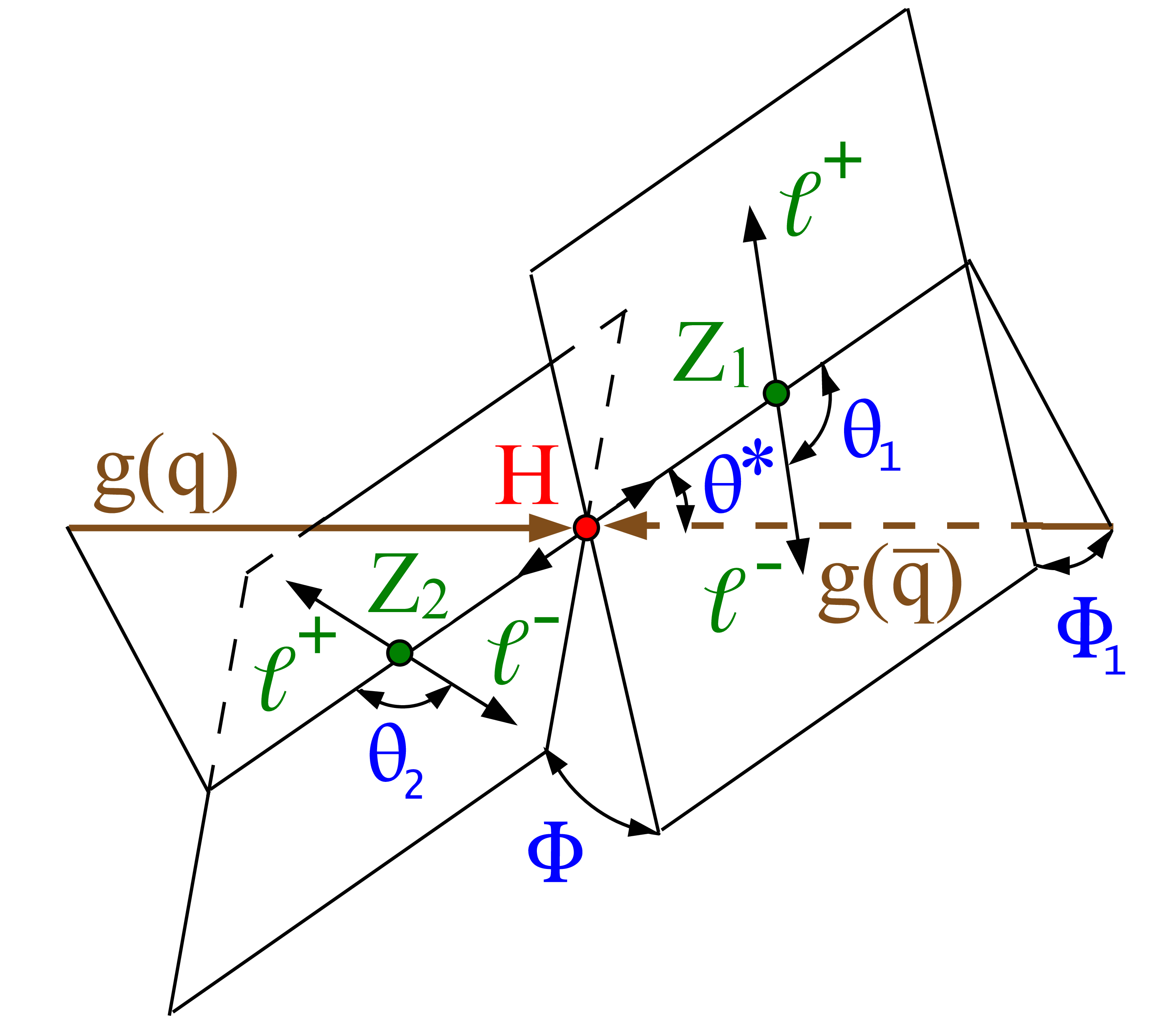
Figure 1:
Schematic representation of the $ \mathrm{g}\mathrm{g}/\mathrm{q}\bar{\mathrm{q}}\to \mathrm{H}\to ZZ\to 4\ell $ process. The five angles depicted in blue are considered in the differential analysis, as detailed in the text. |
png pdf |
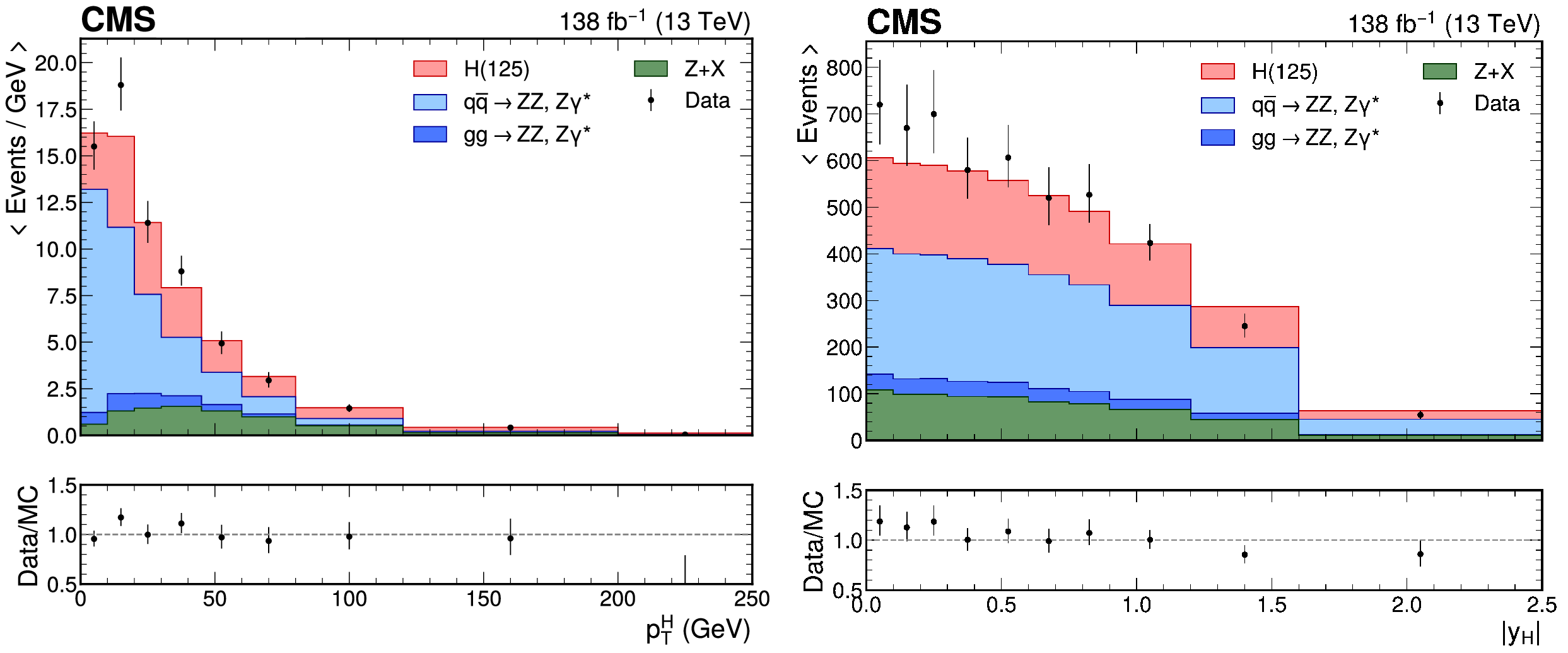
Figure 2:
Reconstructed transverse momentum (left) and rapidity (right) of the four-lepton system. Points with error bars represent the data, solid histograms the predictions from simulation. The $ y $ axes of the top panels have been rescaled to display the number of events per bin, divided by the width of each bin. The lower panels show the ratio of the measured values to the expectations from the simulation. |

png pdf |
Figure 2-a:
Reconstructed transverse momentum of the four-lepton system. Points with error bars represent the data, solid histograms the predictions from simulation. The $ y $ axes of the top panels have been rescaled to display the number of events per bin, divided by the width of each bin. The lower panel shows the ratio of the measured values to the expectations from the simulation. |
png pdf |
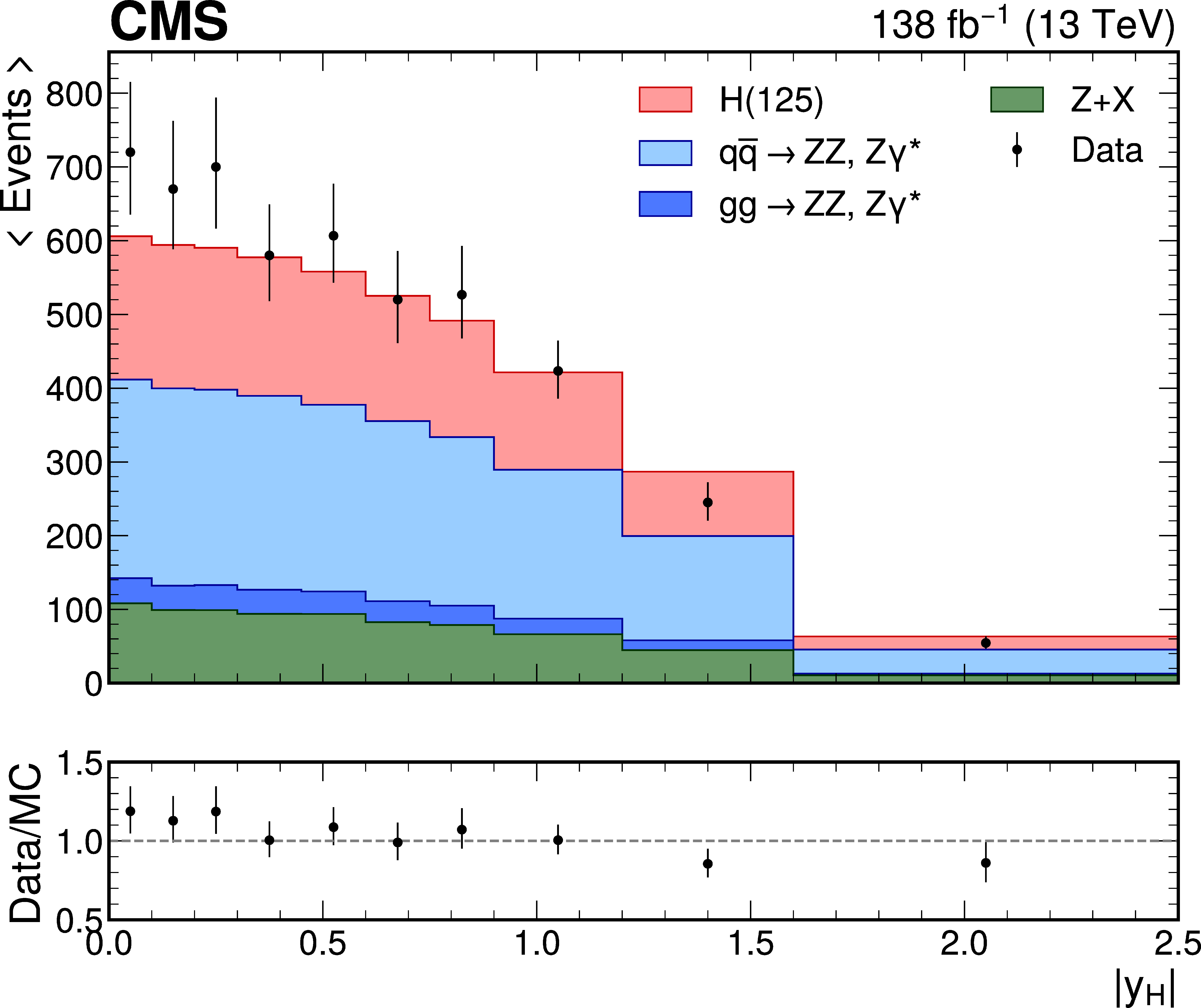
Figure 2-b:
Reconstructed rapidity of the four-lepton system. Points with error bars represent the data, solid histograms the predictions from simulation. The $ y $ axes of the top panels have been rescaled to display the number of events per bin, divided by the width of each bin. The lower panel shows the ratio of the measured values to the expectations from the simulation. |
png pdf |
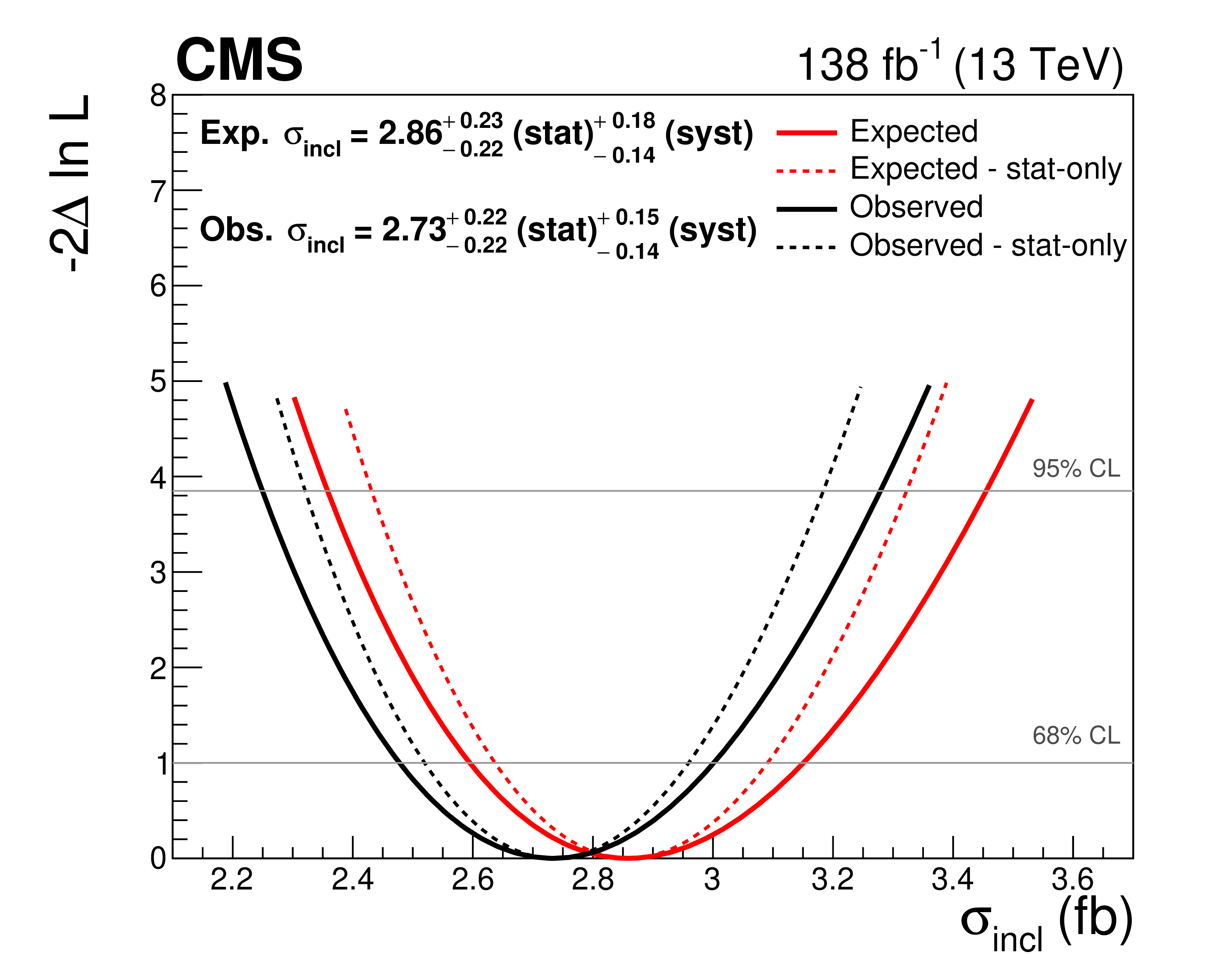
Figure 3:
Log-likelihood scan for the measured inclusive fiducial cross section. The scan is shown with (solid line) and without (dashed line) systematic uncertainties profiled in the fit. |

png pdf |
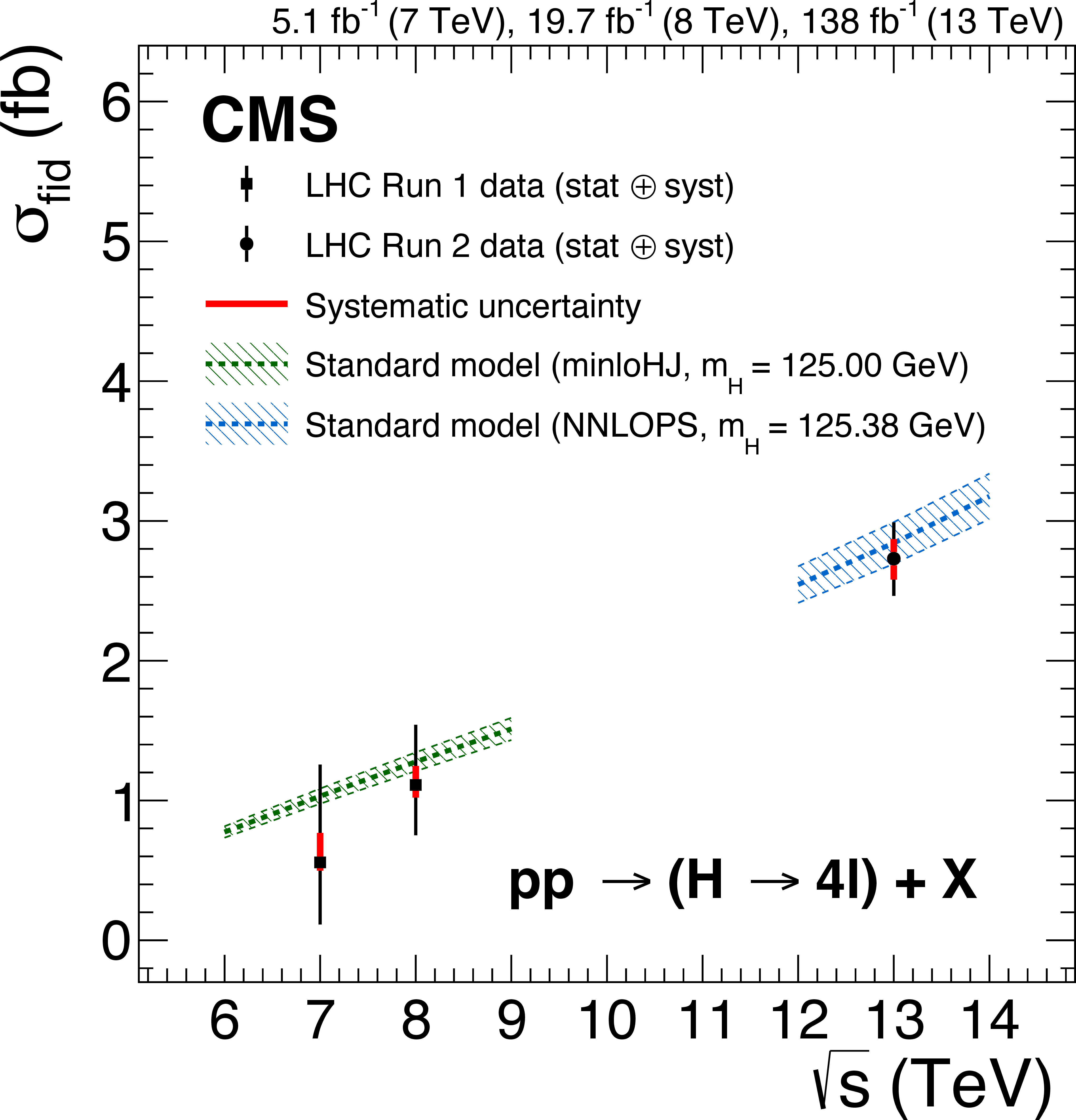
Figure 4:
Measured inclusive fiducial cross section for the various final states (left); and as a function of the center-of-mass energy $ \sqrt{s} $ (right). In the left panel the acceptance and theoretical uncertainties are calculated using POWHEG (blue), NNLOPS (orange), and MadGraph-5_aMC@NLO (pink). The subdominant component of the signal (VBF+VH+ttH) is denoted as XH and is fixed to the SM prediction. In the right panel the acceptance is calculated using POWHEG at $ \sqrt{s}= $ 13 TeV and HRES [127,135] at $ \sqrt{s}= $ 7 and 8 TeV. |

png pdf |
Figure 4-a:
Measured inclusive fiducial cross section for the various final states. The acceptance and theoretical uncertainties are calculated using POWHEG (blue), NNLOPS (orange), and MadGraph-5_aMC@NLO (pink). The subdominant component of the signal (VBF+VH+ttH) is denoted as XH and is fixed to the SM prediction. |
png pdf |
Figure 4-b:
Measured inclusive fiducial cross section as a function of the center-of-mass energy $ \sqrt{s} $. The acceptance is calculated using POWHEG at $ \sqrt{s}= $ 13 TeV and HRES [127,135] at $ \sqrt{s}= $ 7 and 8 TeV. |

png pdf |
Figure 5:
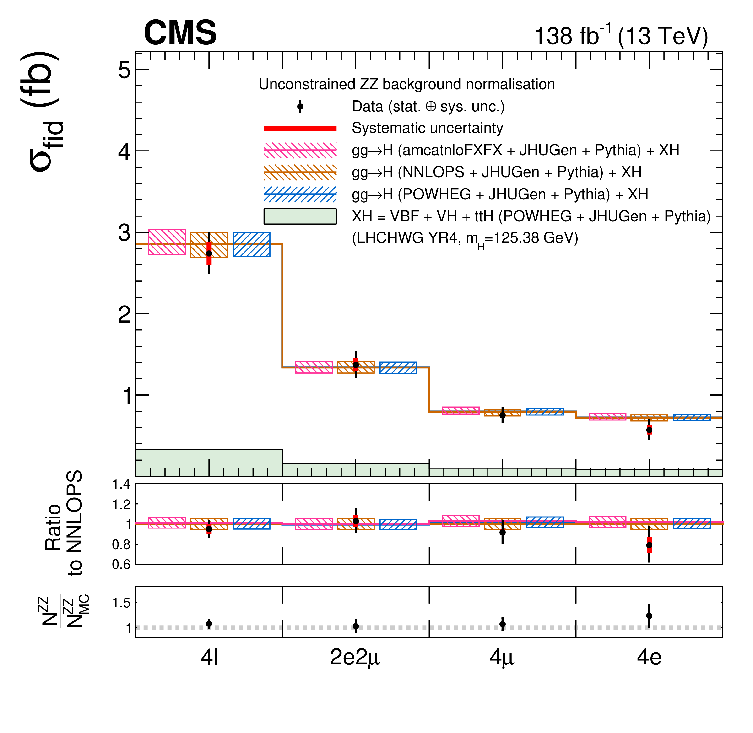
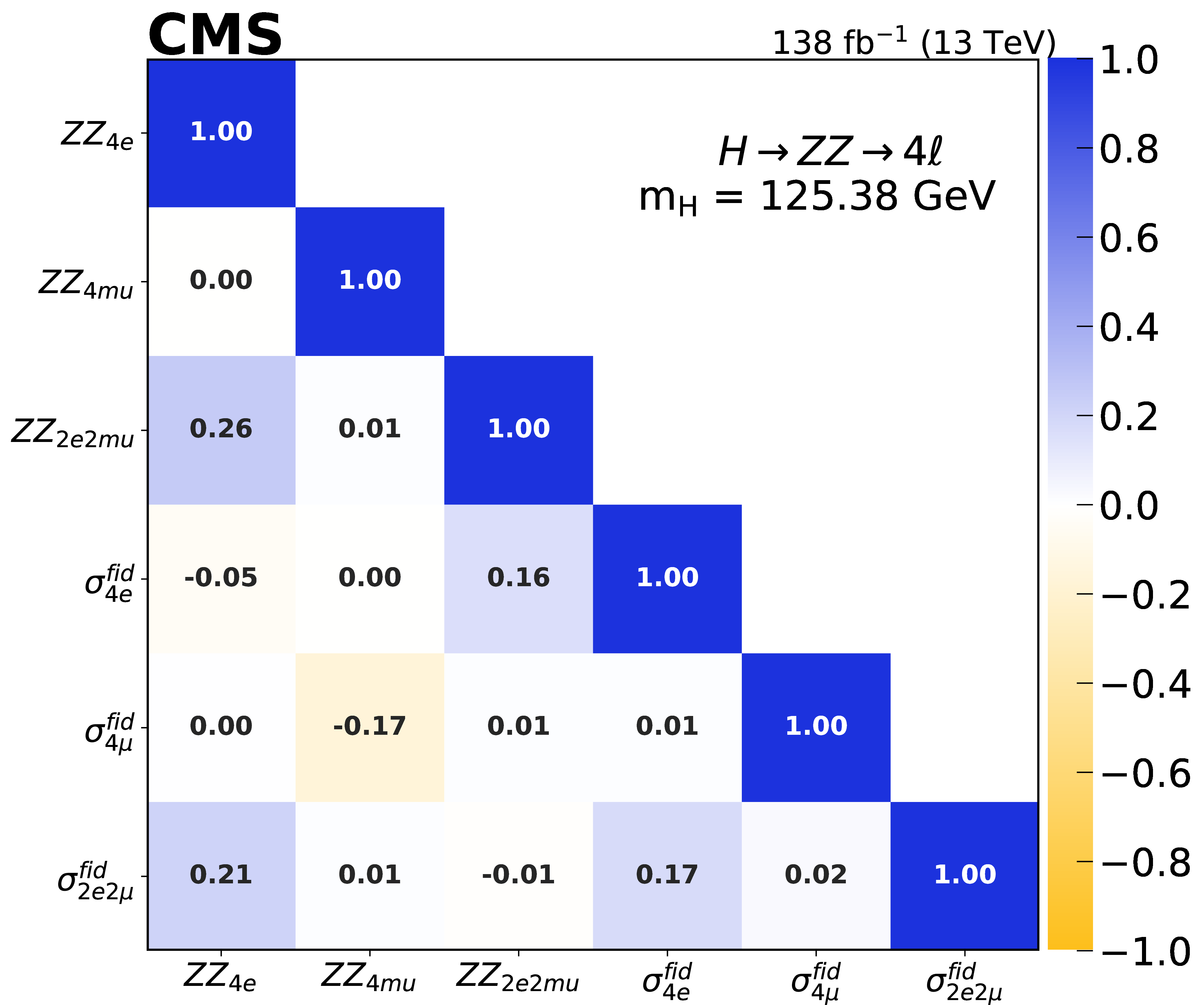
Inclusive fiducial cross section measured for the various final states with the irreducible backgrounds normalization ZZ unconstrained in the fit (left) and the corresponding correlation matrix (right). The acceptance and theoretical uncertainties in the differential bins are calculated using POWHEG (blue), NNLOPS (orange), and MadGraph-5_aMC@NLO (pink). The subdominant component of the signal (VBF+VH+ttH) is denoted as XH and it is fixed to the SM prediction. The ratio of the measured cross section to the theoretical prediction obtained from each generator is shown in the central panel, while the lower panel shows the ratio between the values derived from the measured ZZ normalization and the MC prediction. |
png pdf |
Figure 5-a:
Inclusive fiducial cross section measured for the various final states with the irreducible backgrounds normalization ZZ unconstrained in the fit.The acceptance and theoretical uncertainties in the differential bins are calculated using POWHEG (blue), NNLOPS (orange), and MadGraph-5_aMC@NLO (pink). The subdominant component of the signal (VBF+VH+ttH) is denoted as XH and it is fixed to the SM prediction. The ratio of the measured cross section to the theoretical prediction obtained from each generator is shown in the central panel, while the lower panel shows the ratio between the values derived from the measured ZZ normalization and the MC prediction. |
png pdf |
Figure 5-b:
Correlation matrix for the measurements of the inclusive fiducial cross sections in the various final states and the normalizations of the irreducible ZZ backgrounds, which are unconstrained in the fit. |

png pdf |
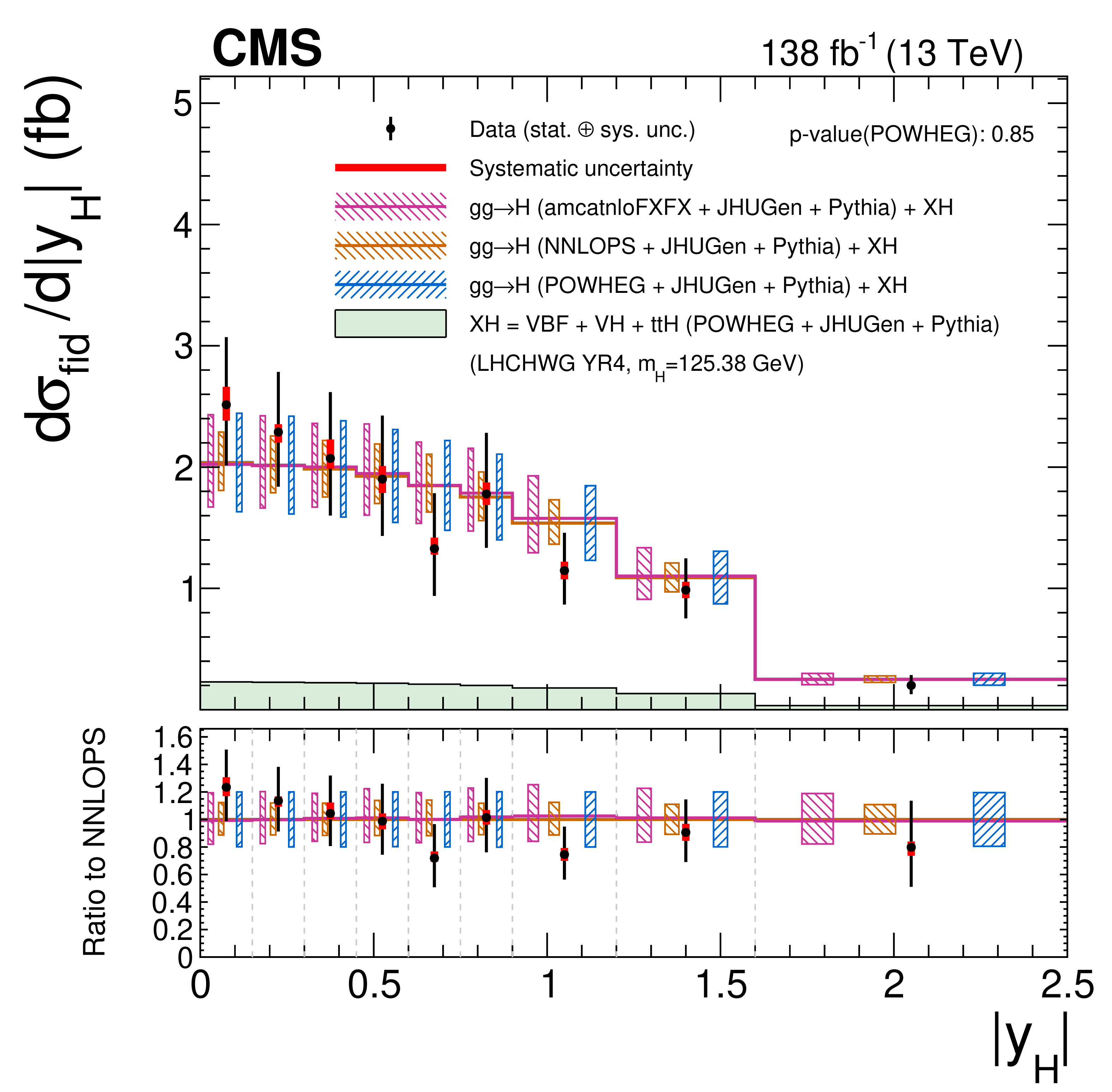
Figure 6:
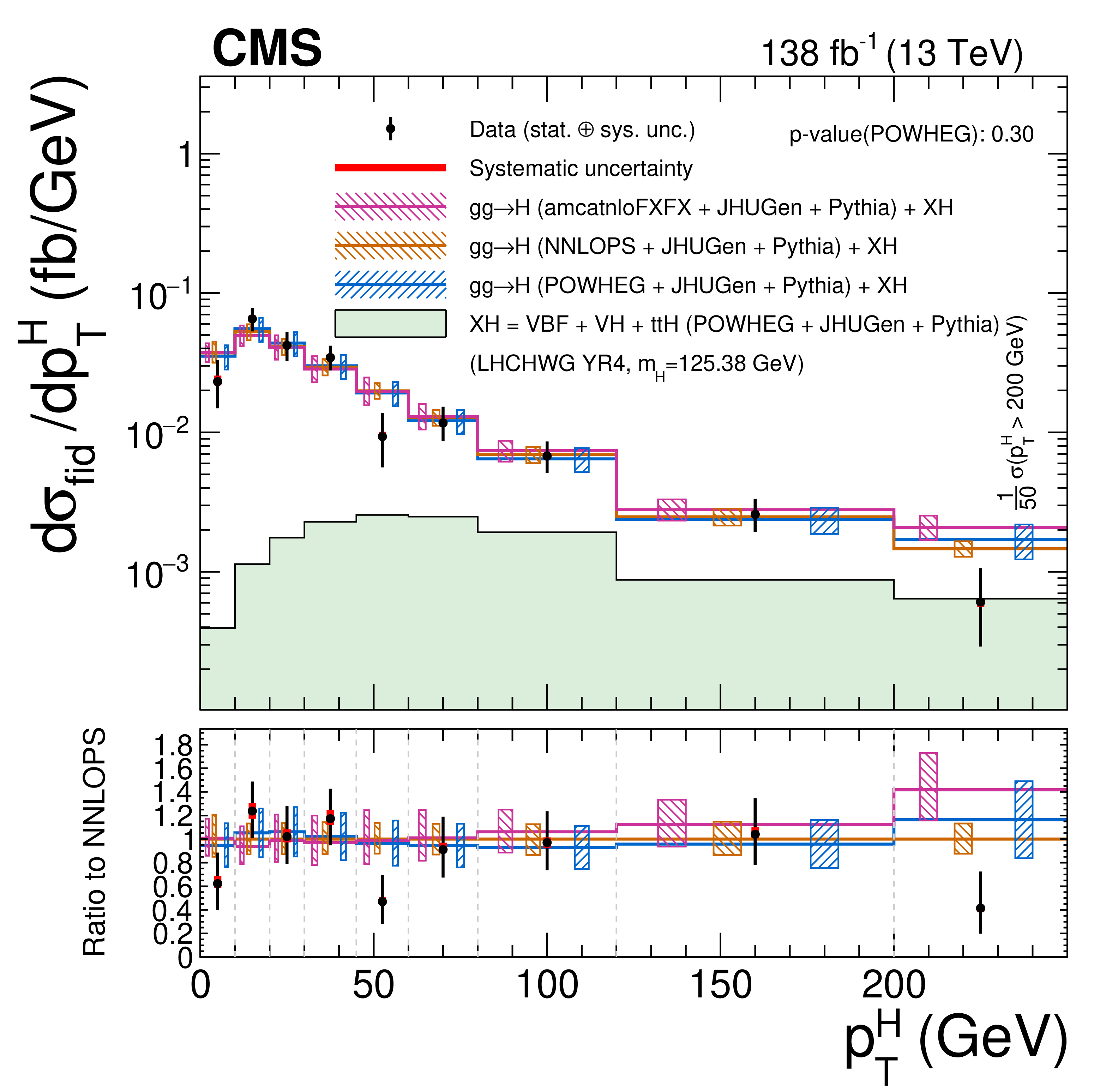
Differential cross sections as functions of the transverse momentum of the Higgs boson $ p_{\mathrm{T}}^{\mathrm{H}} $ (left) and of the rapidity of the Higgs boson $ |y_{\mathrm{H}}| $ (right). The fiducial cross section in the last bin (left) is measured for events with $ p_{\mathrm{T}}^{\mathrm{H}} > $ 200 GeV and normalized to a bin width of 50 GeV. The acceptance and theoretical uncertainties in the differential bins are calculated using the ggH predictions from the POWHEG generator (blue) normalized to next-to- next-to-next-to-leading order ($ \mathrm{N^3LO} $) [34]. The subdominant component of the signal (VBF+VH+ttH) is denoted as XH and is fixed to the SM prediction. The measured cross sections are also compared with the ggH predictions from NNLOPS (orange) and MadGraph-5_aMC@NLO (pink). The hatched areas correspond to the systematic uncertainties in the theoretical predictions. Black points represent the measured fiducial cross sections in each bin, black error bars the total uncertainty in each measurement, red boxes the systematic uncertainties. The lower panels display the ratios of the measured cross sections and of the predictions from POWHEG and MadGraph-5_aMC@NLO to the NNLOPS theoretical predictions. |
png pdf |
Figure 6-a:
Differential cross sections as a function of the transverse momentum of the Higgs boson $ p_{\mathrm{T}}^{\mathrm{H}} $. The fiducial cross section in the last bin is measured for events with $ p_{\mathrm{T}}^{\mathrm{H}} > $ 200 GeV and normalized to a bin width of 50 GeV. The acceptance and theoretical uncertainties in the differential bins are calculated using the ggH predictions from the POWHEG generator (blue) normalized to next-to- next-to-next-to-leading order ($ \mathrm{N^3LO} $) [34]. The subdominant component of the signal (VBF+VH+ttH) is denoted as XH and is fixed to the SM prediction. The measured cross sections are also compared with the ggH predictions from NNLOPS (orange) and MadGraph-5_aMC@NLO (pink). The hatched areas correspond to the systematic uncertainties in the theoretical predictions. Black points represent the measured fiducial cross sections in each bin, black error bars the total uncertainty in each measurement, red boxes the systematic uncertainties. The lower panel displays the ratios of the measured cross sections and of the predictions from POWHEG and MadGraph-5_aMC@NLO to the NNLOPS theoretical predictions. |
png pdf |
Figure 6-b:
Differential cross sections as a function of the rapidity of the Higgs boson $ |y_{\mathrm{H}}| $. The acceptance and theoretical uncertainties in the differential bins are calculated using the ggH predictions from the POWHEG generator (blue) normalized to next-to- next-to-next-to-leading order ($ \mathrm{N^3LO} $) [34]. The subdominant component of the signal (VBF+VH+ttH) is denoted as XH and is fixed to the SM prediction. The measured cross sections are also compared with the ggH predictions from NNLOPS (orange) and MadGraph-5_aMC@NLO (pink). The hatched areas correspond to the systematic uncertainties in the theoretical predictions. Black points represent the measured fiducial cross sections in each bin, black error bars the total uncertainty in each measurement, red boxes the systematic uncertainties. The lower panel displays the ratios of the measured cross sections and of the predictions from POWHEG and MadGraph-5_aMC@NLO to the NNLOPS theoretical predictions. |
png pdf |
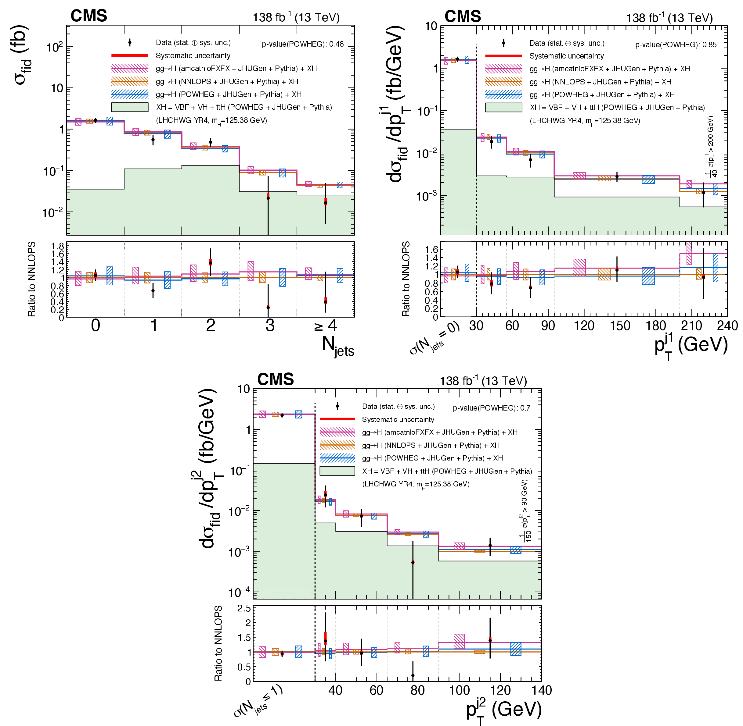
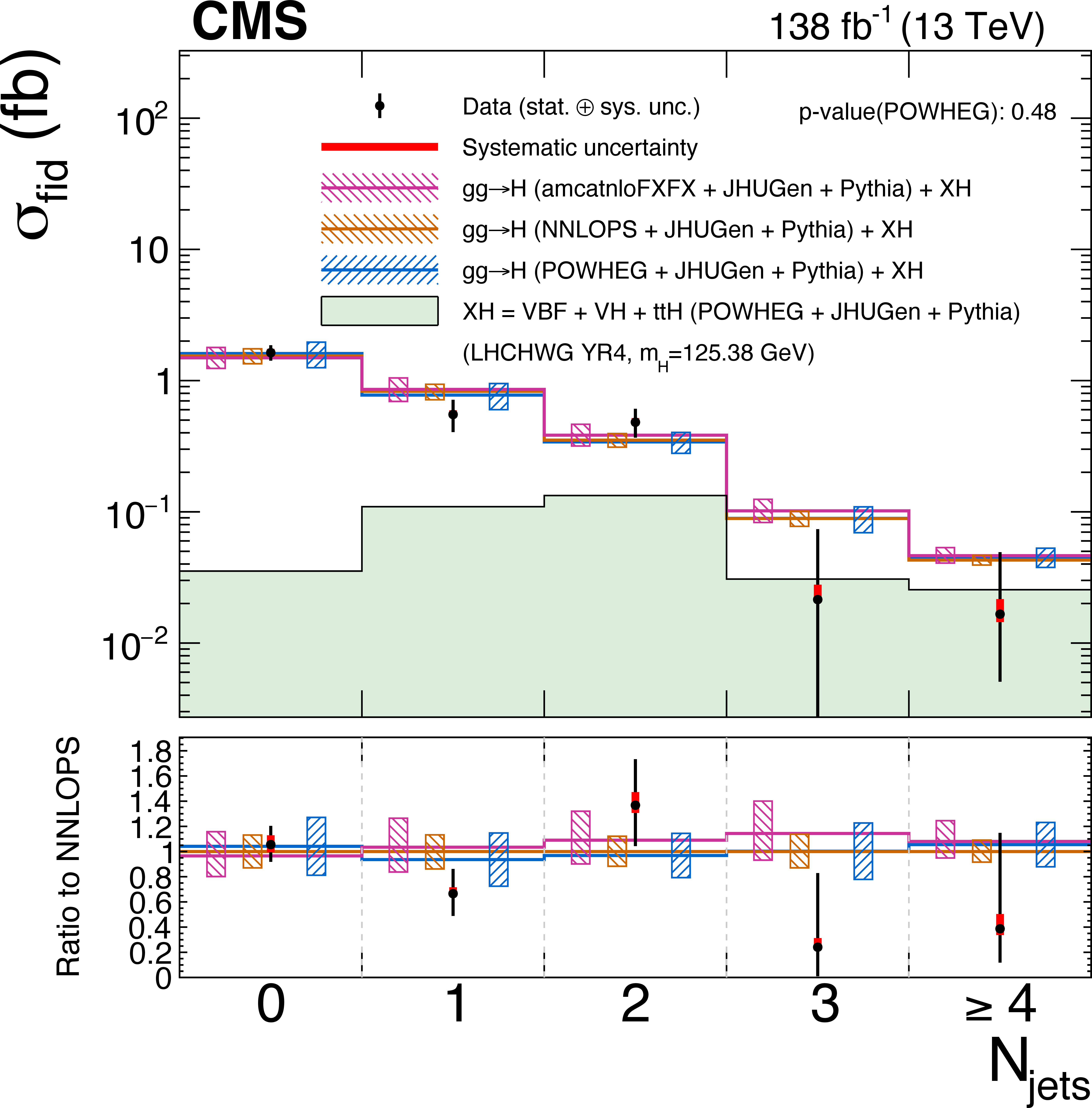
Figure 7:
Differential cross sections as functions of the number of jets in the event (upper left) and of the $ p_{\mathrm{T}} $ of the leading (upper right) and subleading (lower) jet. Upper right: the fiducial cross section in the last bin is measured for events with $ p_{\mathrm{T}}^{\text{j1}} > $ 200 GeV and normalized to a bin width of 40 GeV. The first bin comprises all events with less than one jet, for which $ p_{\mathrm{T}}^{\text{j1}} $ is undefined. Lower: the fiducial cross section in the last bin is measured for events with $ p_{\mathrm{T}}^{\text{j2}} > $ 90 GeV and normalized to a bin width of 150 GeV. The first bin comprises all events with less than two jet, for which $ p_{\mathrm{T}}^{\text{j2}} $ is undefined. The acceptance and theoretical uncertainties in the differential bins are calculated using the ggH predictions from the POWHEG generator (blue) normalized to $ \mathrm{N^3LO} $. The subdominant component of the signal (VBF+VH+ttH) is denoted as XH and is fixed to the SM prediction. The measured cross sections are also compared with the ggH predictions from NNLOPS (orange) and MadGraph-5_aMC@NLO (pink). The hatched areas correspond to the systematic uncertainties in the theoretical predictions. Black points represent the measured fiducial cross sections in each bin, black error bars the total uncertainty in each measurement, red boxes the systematic uncertainties. The lower panels display the ratios of the measured cross sections and of the predictions from POWHEG and MadGraph-5_aMC@NLO to the NNLOPS theoretical predictions. |
png pdf |
Figure 7-a:
Differential cross sections as a function of the number of jets in the event. The acceptance and theoretical uncertainties in the differential bins are calculated using the ggH predictions from the POWHEG generator (blue) normalized to $ \mathrm{N^3LO} $. The subdominant component of the signal (VBF+VH+ttH) is denoted as XH and is fixed to the SM prediction. The measured cross sections are also compared with the ggH predictions from NNLOPS (orange) and MadGraph-5_aMC@NLO (pink). The hatched areas correspond to the systematic uncertainties in the theoretical predictions. Black points represent the measured fiducial cross sections in each bin, black error bars the total uncertainty in each measurement, red boxes the systematic uncertainties. The lower panel displays the ratios of the measured cross sections and of the predictions from POWHEG and MadGraph-5_aMC@NLO to the NNLOPS theoretical predictions. |

png pdf |
Figure 7-b:
Differential cross sections as a function of the $ p_{\mathrm{T}} $ of the leading jet. The fiducial cross section in the last bin is measured for events with $ p_{\mathrm{T}}^{\text{j1}} > $ 200 GeV and normalized to a bin width of 40 GeV. The first bin comprises all events with less than one jet, for which $ p_{\mathrm{T}}^{\text{j1}} $ is undefined. The acceptance and theoretical uncertainties in the differential bins are calculated using the ggH predictions from the POWHEG generator (blue) normalized to $ \mathrm{N^3LO} $. The subdominant component of the signal (VBF+VH+ttH) is denoted as XH and is fixed to the SM prediction. The measured cross sections are also compared with the ggH predictions from NNLOPS (orange) and MadGraph-5_aMC@NLO (pink). The hatched areas correspond to the systematic uncertainties in the theoretical predictions. Black points represent the measured fiducial cross sections in each bin, black error bars the total uncertainty in each measurement, red boxes the systematic uncertainties. The lower panel displays the ratios of the measured cross sections and of the predictions from POWHEG and MadGraph-5_aMC@NLO to the NNLOPS theoretical predictions. |

png pdf |
Figure 7-c:
Differential cross sections as a function of the $ p_{\mathrm{T}} $ of the subleading jet. The fiducial cross section in the last bin is measured for events with $ p_{\mathrm{T}}^{\text{j2}} > $ 90 GeV and normalized to a bin width of 150 GeV. The first bin comprises all events with less than two jet, for which $ p_{\mathrm{T}}^{\text{j2}} $ is undefined. The acceptance and theoretical uncertainties in the differential bins are calculated using the ggH predictions from the POWHEG generator (blue) normalized to $ \mathrm{N^3LO} $. The subdominant component of the signal (VBF+VH+ttH) is denoted as XH and is fixed to the SM prediction. The measured cross sections are also compared with the ggH predictions from NNLOPS (orange) and MadGraph-5_aMC@NLO (pink). The hatched areas correspond to the systematic uncertainties in the theoretical predictions. Black points represent the measured fiducial cross sections in each bin, black error bars the total uncertainty in each measurement, red boxes the systematic uncertainties. The lower panel displays the ratios of the measured cross sections and of the predictions from POWHEG and MadGraph-5_aMC@NLO to the NNLOPS theoretical predictions. |
png pdf |
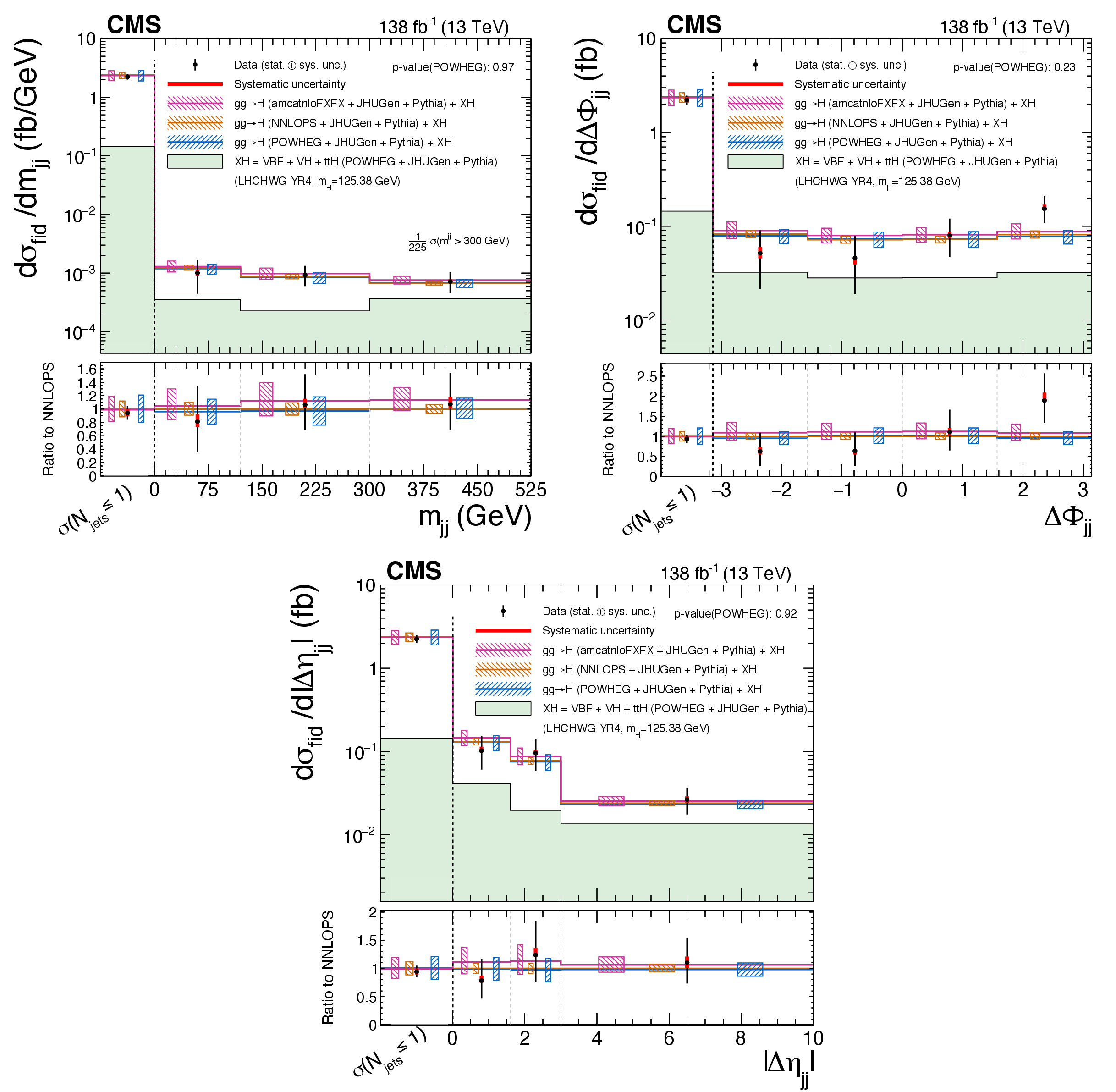
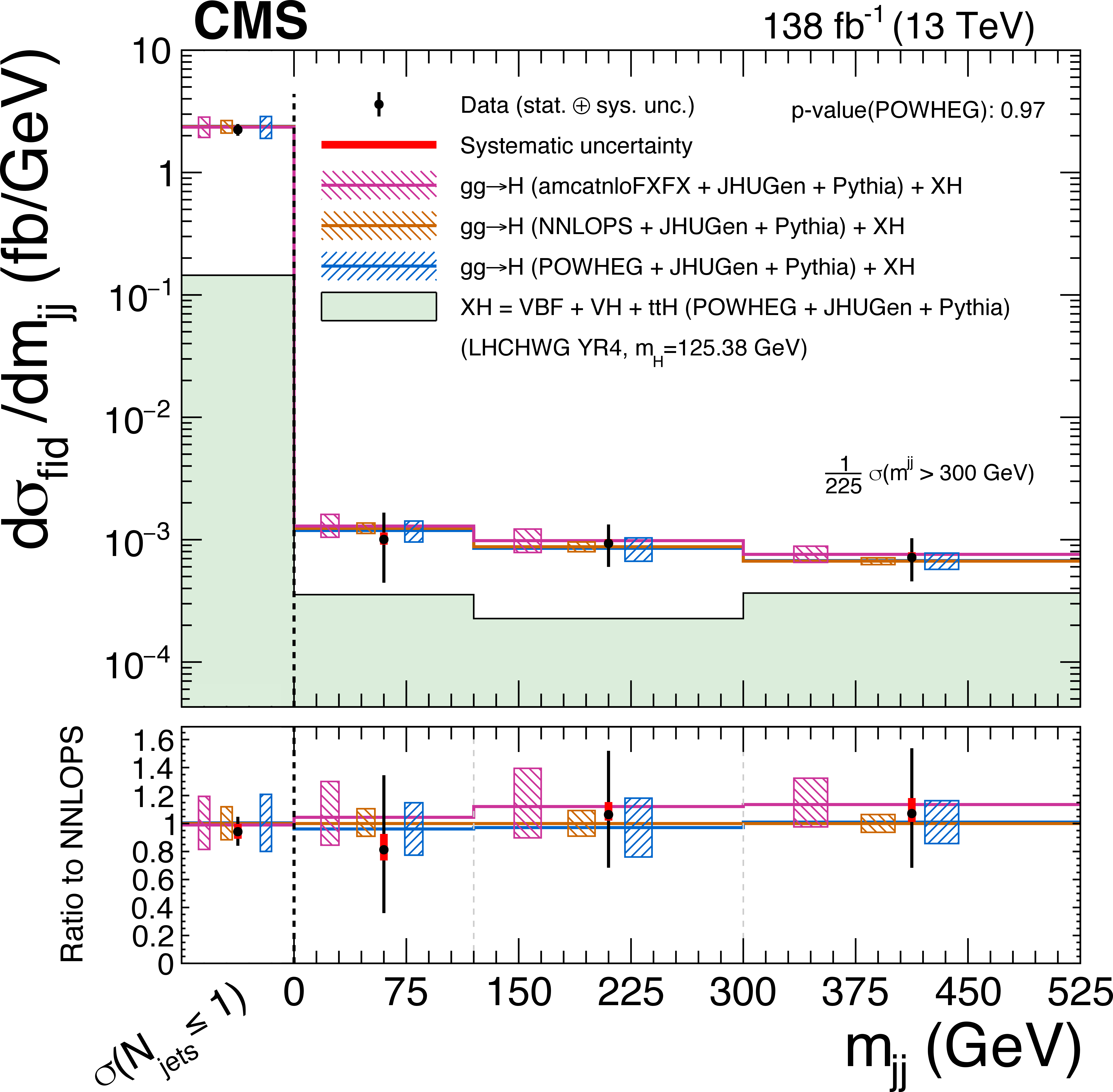
Figure 8:
Differential cross sections as functions of the invariant mass $ m_\text{jj} $ (upper left), the difference in azimuthal angle $ \Delta\phi_{\text{jj}} $ (upper right) the difference in pseudorapidity $ |\Delta\eta_\text{jj}| $ (lower) of the dijet system. Upper Left: the fiducial cross section in the last bin is measured for events with $ m_\text{jj} > $ 300 GeV and normalized to a bin width of 225 GeV. The first bin comprises all events with less than two jets, for which $ m_\text{jj} $ is undefined. Upper right: the first bin comprises all events with less than two jet, for which $ |\Delta\phi_\text{jj}| $ is undefined. Lower: the first bin comprises all events with less than two jet, for which $ |\Delta\eta_\text{jj}| $ is undefined. The acceptance and theoretical uncertainties in the differential bins are calculated using the ggH predictions from the POWHEG generator (blue) normalized to $ \mathrm{N^3LO} $. The subdominant component of the signal (VBF+VH+ttH) is denoted as XH and is fixed to the SM prediction. The measured cross sections are also compared with the ggH predictions from NNLOPS (orange) and MadGraph-5_aMC@NLO (pink). The hatched areas correspond to the systematic uncertainties in the theoretical predictions. Black points represent the measured fiducial cross sections in each bin, black error bars the total uncertainty in each measurement, red boxes the systematic uncertainties. The lower panels display the ratios of the measured cross sections and of the predictions from POWHEG and MadGraph-5_aMC@NLO to the NNLOPS theoretical predictions. |
png pdf |
Figure 8-a:
Differential cross sections as a function of the invariant mass $ m_\text{jj} $ of the dijet system. The fiducial cross section in the last bin is measured for events with $ m_\text{jj} > $ 300 GeV and normalized to a bin width of 225 GeV. The first bin comprises all events with less than two jets, for which $ m_\text{jj} $ is undefined. The acceptance and theoretical uncertainties in the differential bins are calculated using the ggH predictions from the POWHEG generator (blue) normalized to $ \mathrm{N^3LO} $. The subdominant component of the signal (VBF+VH+ttH) is denoted as XH and is fixed to the SM prediction. The measured cross sections are also compared with the ggH predictions from NNLOPS (orange) and MadGraph-5_aMC@NLO (pink). The hatched areas correspond to the systematic uncertainties in the theoretical predictions. Black points represent the measured fiducial cross sections in each bin, black error bars the total uncertainty in each measurement, red boxes the systematic uncertainties. The lower panel displays the ratios of the measured cross sections and of the predictions from POWHEG and MadGraph-5_aMC@NLO to the NNLOPS theoretical predictions. |

png pdf |
Figure 8-b:
Differential cross sections as a function of the difference in azimuthal angle $ \Delta\phi_{\text{jj}} $ of the dijet system. The first bin comprises all events with less than two jet, for which $ |\Delta\phi_\text{jj}| $ is undefined. The acceptance and theoretical uncertainties in the differential bins are calculated using the ggH predictions from the POWHEG generator (blue) normalized to $ \mathrm{N^3LO} $. The subdominant component of the signal (VBF+VH+ttH) is denoted as XH and is fixed to the SM prediction. The measured cross sections are also compared with the ggH predictions from NNLOPS (orange) and MadGraph-5_aMC@NLO (pink). The hatched areas correspond to the systematic uncertainties in the theoretical predictions. Black points represent the measured fiducial cross sections in each bin, black error bars the total uncertainty in each measurement, red boxes the systematic uncertainties. The lower panel displays the ratios of the measured cross sections and of the predictions from POWHEG and MadGraph-5_aMC@NLO to the NNLOPS theoretical predictions. |

png pdf |
Figure 8-c:
Differential cross sections as a function of the difference in pseudorapidity $ |\Delta\eta_\text{jj}| $ of the dijet system. The first bin comprises all events with less than two jet, for which $ |\Delta\eta_\text{jj}| $ is undefined. The acceptance and theoretical uncertainties in the differential bins are calculated using the ggH predictions from the POWHEG generator (blue) normalized to $ \mathrm{N^3LO} $. The subdominant component of the signal (VBF+VH+ttH) is denoted as XH and is fixed to the SM prediction. The measured cross sections are also compared with the ggH predictions from NNLOPS (orange) and MadGraph-5_aMC@NLO (pink). The hatched areas correspond to the systematic uncertainties in the theoretical predictions. Black points represent the measured fiducial cross sections in each bin, black error bars the total uncertainty in each measurement, red boxes the systematic uncertainties. The lower panel displays the ratios of the measured cross sections and of the predictions from POWHEG and MadGraph-5_aMC@NLO to the NNLOPS theoretical predictions. |

png pdf |
Figure 9:
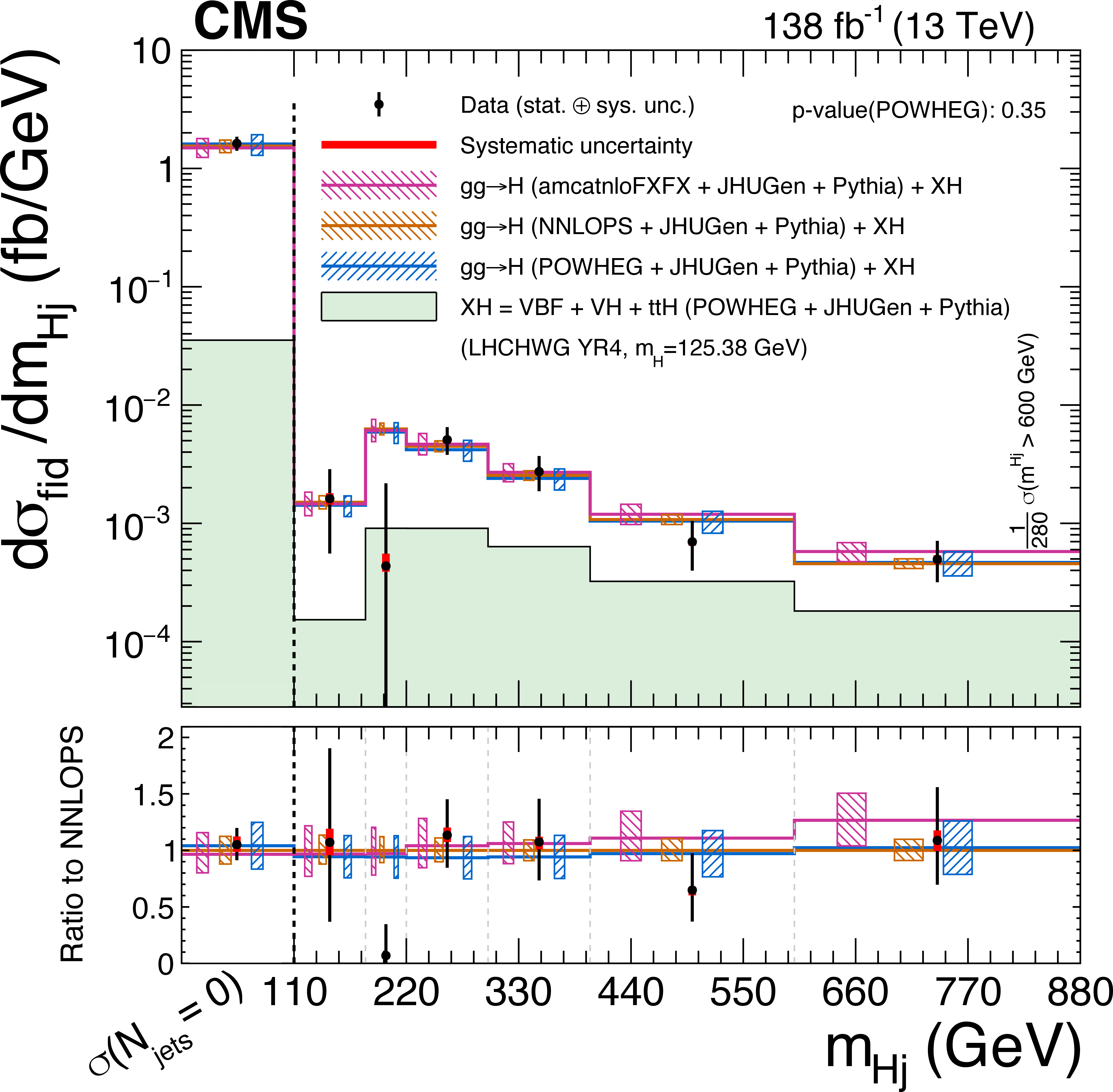
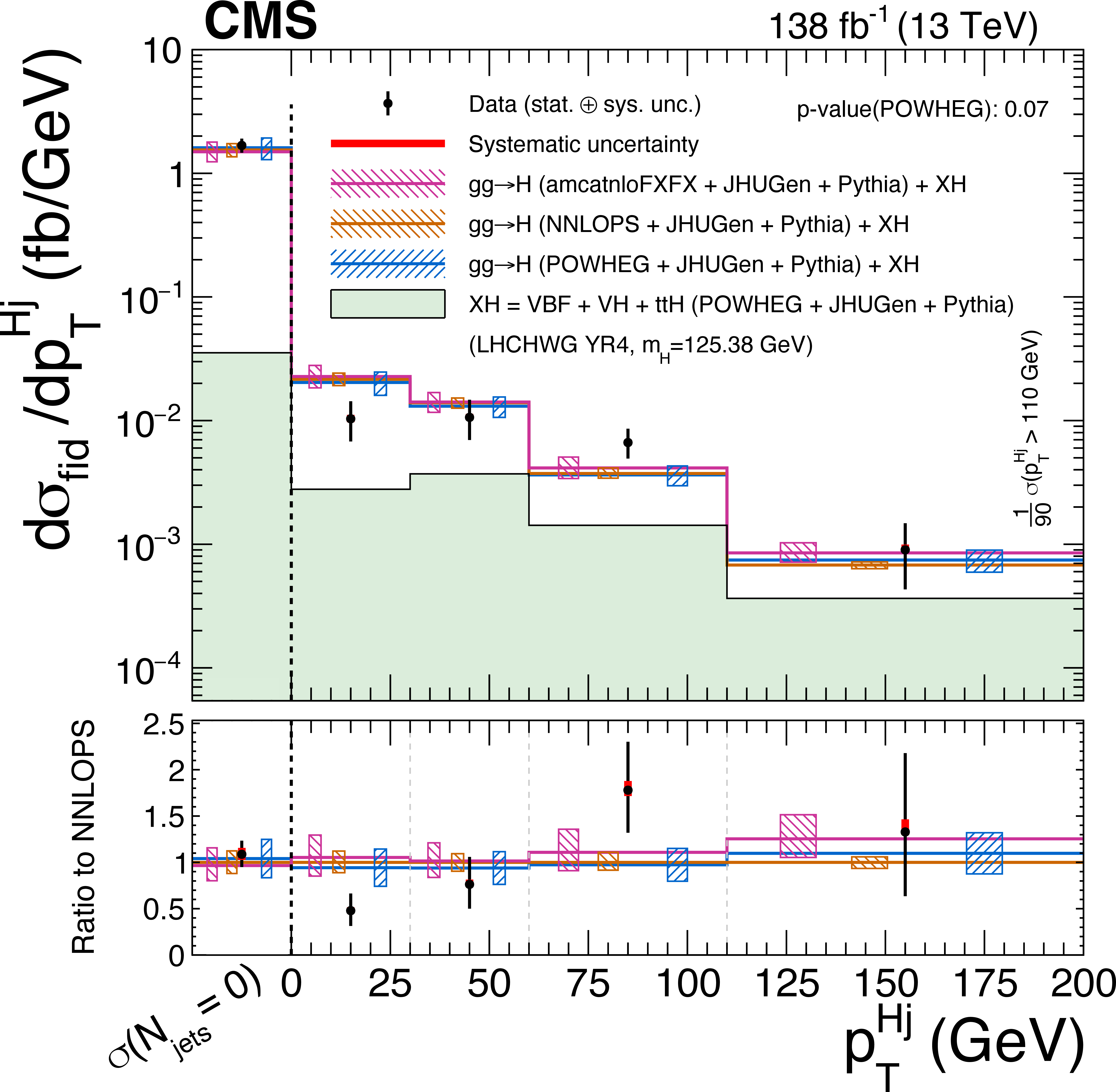
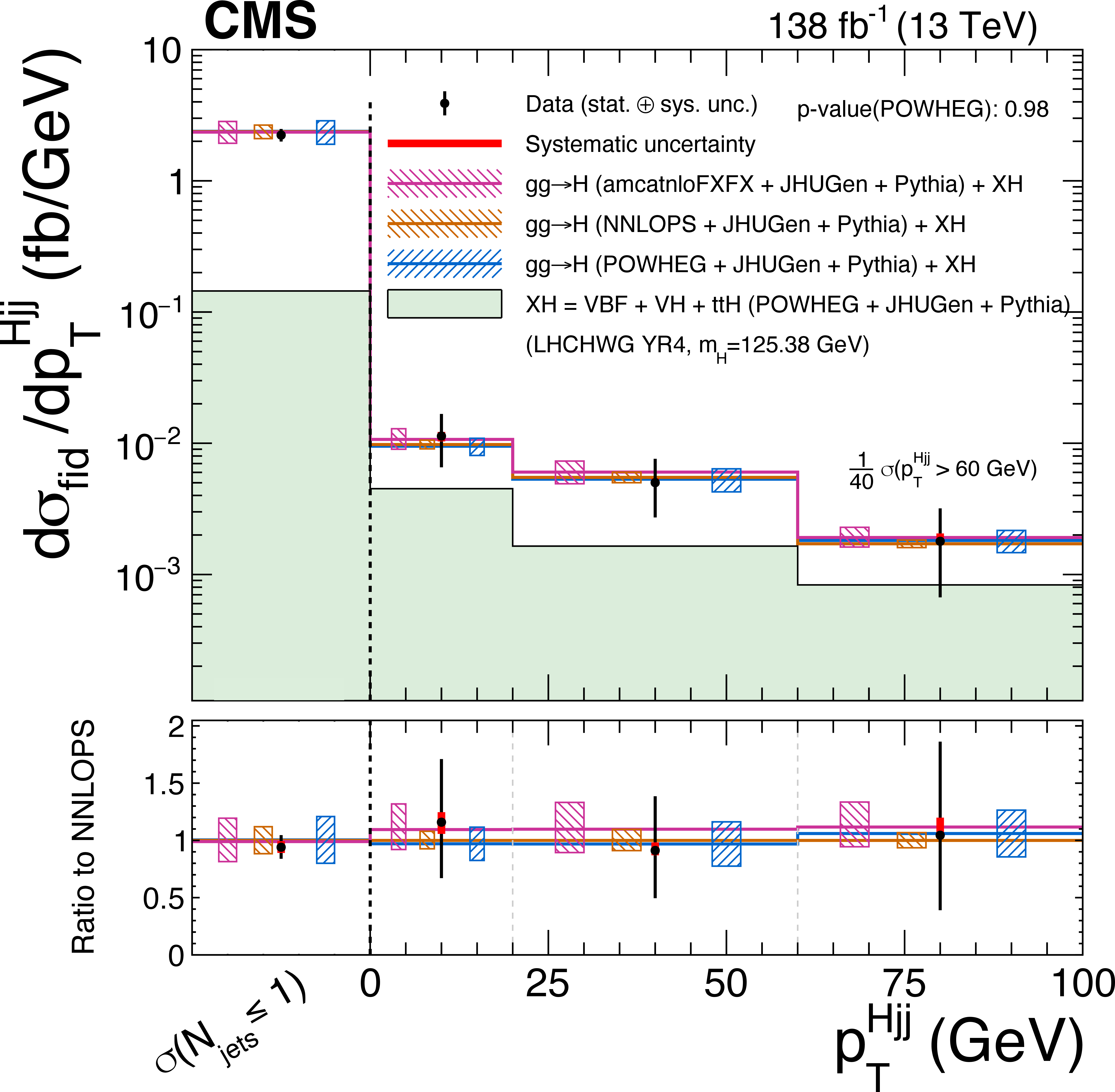
Upper left: differential cross sections as functions of the invariant mass of the $ \mathrm{H}+j $ system $ m_{\mathrm{H} j} $, where j is the leading jet in the event. The fiducial cross section in the last bin is measured for events with $ m_{\mathrm{H} j} > $ 600 GeV and normalized to a bin width of 280 GeV. The first bin comprises all events with less than one jet, for which $ m_{\mathrm{H} j} $ is undefined. Upper right: differential cross sections as functions of the transverse momentum of the $ \mathrm{H}+j $ system $ p_{\mathrm{T}}^{\mathrm{H} j} $. The fiducial cross section in the last bin is measured for events with $ p_{\mathrm{T}}^{\mathrm{H} j} > $ 110 GeV and normalized to a bin width of 90 GeV. The first bin comprises all events with less than one jet, for which $ p_{\mathrm{T}}^{\mathrm{H} j} $ is undefined. Lower: differential cross sections as functions of the transverse momentum of the $ \mathrm{H}+jj $ system $ p_{\mathrm{T}}^{\mathrm{H} jj} $. The fiducial cross section in the last bin is measured for events with $ p_{\mathrm{T}}^{\mathrm{H} jj} > $ 60 GeV and normalized to a bin width of 40 GeV. The first bin comprises all events with less than two jet, for which $ p_{\mathrm{T}}^{\mathrm{H} jj} $ is undefined. The acceptance and theoretical uncertainties in the differential bins are calculated using the ggH predictions from the POWHEG generator (blue) normalized to $ \mathrm{N^3LO} $. The subdominant component of the signal (VBF+VH+ttH) is denoted as XH and is fixed to the SM prediction. The measured cross sections are also compared with the ggH predictions from NNLOPS (orange) and MadGraph-5_aMC@NLO (pink). The hatched areas correspond to the systematic uncertainties in the theoretical predictions. Black points represent the measured fiducial cross sections in each bin, black error bars the total uncertainty in each measurement, red boxes the systematic uncertainties. The lower panels display the ratios of the measured cross sections and of the predictions from POWHEG and MadGraph-5_aMC@NLO to the NNLOPS theoretical predictions. |
png pdf |
Figure 9-a:
Differential cross sections as functions of the invariant mass of the $ \mathrm{H}+j $ system $ m_{\mathrm{H} j} $, where j is the leading jet in the event. The fiducial cross section in the last bin is measured for events with $ m_{\mathrm{H} j} > $ 600 GeV and normalized to a bin width of 280 GeV. The first bin comprises all events with less than one jet, for which $ m_{\mathrm{H} j} $ is undefined. The acceptance and theoretical uncertainties in the differential bins are calculated using the ggH predictions from the POWHEG generator (blue) normalized to $ \mathrm{N^3LO} $. The subdominant component of the signal (VBF+VH+ttH) is denoted as XH and is fixed to the SM prediction. The measured cross sections are also compared with the ggH predictions from NNLOPS (orange) and MadGraph-5_aMC@NLO (pink). The hatched areas correspond to the systematic uncertainties in the theoretical predictions. Black points represent the measured fiducial cross sections in each bin, black error bars the total uncertainty in each measurement, red boxes the systematic uncertainties. The lower panel displays the ratios of the measured cross sections and of the predictions from POWHEG and MadGraph-5_aMC@NLO to the NNLOPS theoretical predictions. |
png pdf |
Figure 9-b:
Differential cross sections as functions of the transverse momentum of the $ \mathrm{H}+j $ system $ p_{\mathrm{T}}^{\mathrm{H} j} $. The fiducial cross section in the last bin is measured for events with $ p_{\mathrm{T}}^{\mathrm{H} j} > $ 110 GeV and normalized to a bin width of 90 GeV. The first bin comprises all events with less than one jet, for which $ p_{\mathrm{T}}^{\mathrm{H} j} $ is undefined. The acceptance and theoretical uncertainties in the differential bins are calculated using the ggH predictions from the POWHEG generator (blue) normalized to $ \mathrm{N^3LO} $. The subdominant component of the signal (VBF+VH+ttH) is denoted as XH and is fixed to the SM prediction. The measured cross sections are also compared with the ggH predictions from NNLOPS (orange) and MadGraph-5_aMC@NLO (pink). The hatched areas correspond to the systematic uncertainties in the theoretical predictions. Black points represent the measured fiducial cross sections in each bin, black error bars the total uncertainty in each measurement, red boxes the systematic uncertainties. The lower panel displays the ratios of the measured cross sections and of the predictions from POWHEG and MadGraph-5_aMC@NLO to the NNLOPS theoretical predictions. |
png pdf |
Figure 9-c:
Differential cross sections as functions of the transverse momentum of the $ \mathrm{H}+jj $ system $ p_{\mathrm{T}}^{\mathrm{H} jj} $. The fiducial cross section in the last bin is measured for events with $ p_{\mathrm{T}}^{\mathrm{H} jj} > $ 60 GeV and normalized to a bin width of 40 GeV. The first bin comprises all events with less than two jet, for which $ p_{\mathrm{T}}^{\mathrm{H} jj} $ is undefined. The acceptance and theoretical uncertainties in the differential bins are calculated using the ggH predictions from the POWHEG generator (blue) normalized to $ \mathrm{N^3LO} $. The subdominant component of the signal (VBF+VH+ttH) is denoted as XH and is fixed to the SM prediction. The measured cross sections are also compared with the ggH predictions from NNLOPS (orange) and MadGraph-5_aMC@NLO (pink). The hatched areas correspond to the systematic uncertainties in the theoretical predictions. Black points represent the measured fiducial cross sections in each bin, black error bars the total uncertainty in each measurement, red boxes the systematic uncertainties. The lower panel displays the ratios of the measured cross sections and of the predictions from POWHEG and MadGraph-5_aMC@NLO to the NNLOPS theoretical predictions. |

png pdf |
Figure 10:
Left: differential cross sections as functions of the rapidity-weighed jet veto $ \mathcal{T}_{\text{C}}^{\text{max}} $. The fiducial cross section in the last bin is measured for events with $ \mathcal{T}_{\text{C}}^{\text{max}} > $ 80 GeV and normalized to a bin width of 70 GeV. The first bin comprises all events in the 0-jet phase space region redefined as a function of $ \mathcal{T}_{\text{C}}^{\text{max}} $, i.e.,, events with less than one jet, for which $ \mathcal{T}_{\text{C}}^{\text{max}} $ is undefined, and events with $ \mathcal{T}_{\text{C}}^{\text{max}} < $ 15 GeV. Right: differential cross sections as functions of the rapidity-weighed jet veto $ \mathcal{T}_{\text{B}}^{\text{max}} $. The fiducial cross section in the last bin is measured for events with $ \mathcal{T}_{\text{B}}^{\text{max}} > $ 150 GeV and normalized to a bin width of 150 GeV. The first bin comprises all events in the 0-jet phase space region redefined as a function of $ \mathcal{T}_{\text{B}}^{\text{max}} $, i.e.,, events with less than one jet, for which $ \mathcal{T}_{\text{B}}^{\text{max}} $ is undefined, and events with $ \mathcal{T}_{\text{B}}^{\text{max}} < $ 30 GeV. The acceptance and theoretical uncertainties in the differential bins are calculated using the ggH predictions from the POWHEG generator (blue) normalized to $ \mathrm{N^3LO} $. The subdominant component of the signal (VBF+VH+ttH) is denoted as XH and is fixed to the SM prediction. The measured cross sections are also compared with the ggH predictions from NNLOPS (orange) and MadGraph-5_aMC@NLO (pink). The hatched areas correspond to the systematic uncertainties in the theoretical predictions. Black points represent the measured fiducial cross sections in each bin, black error bars the total uncertainty in each measurement, red boxes the systematic uncertainties. The lower panels display the ratios of the measured cross sections and of the predictions from POWHEG and MadGraph-5_aMC@NLO to the NNLOPS theoretical predictions. |
png pdf |
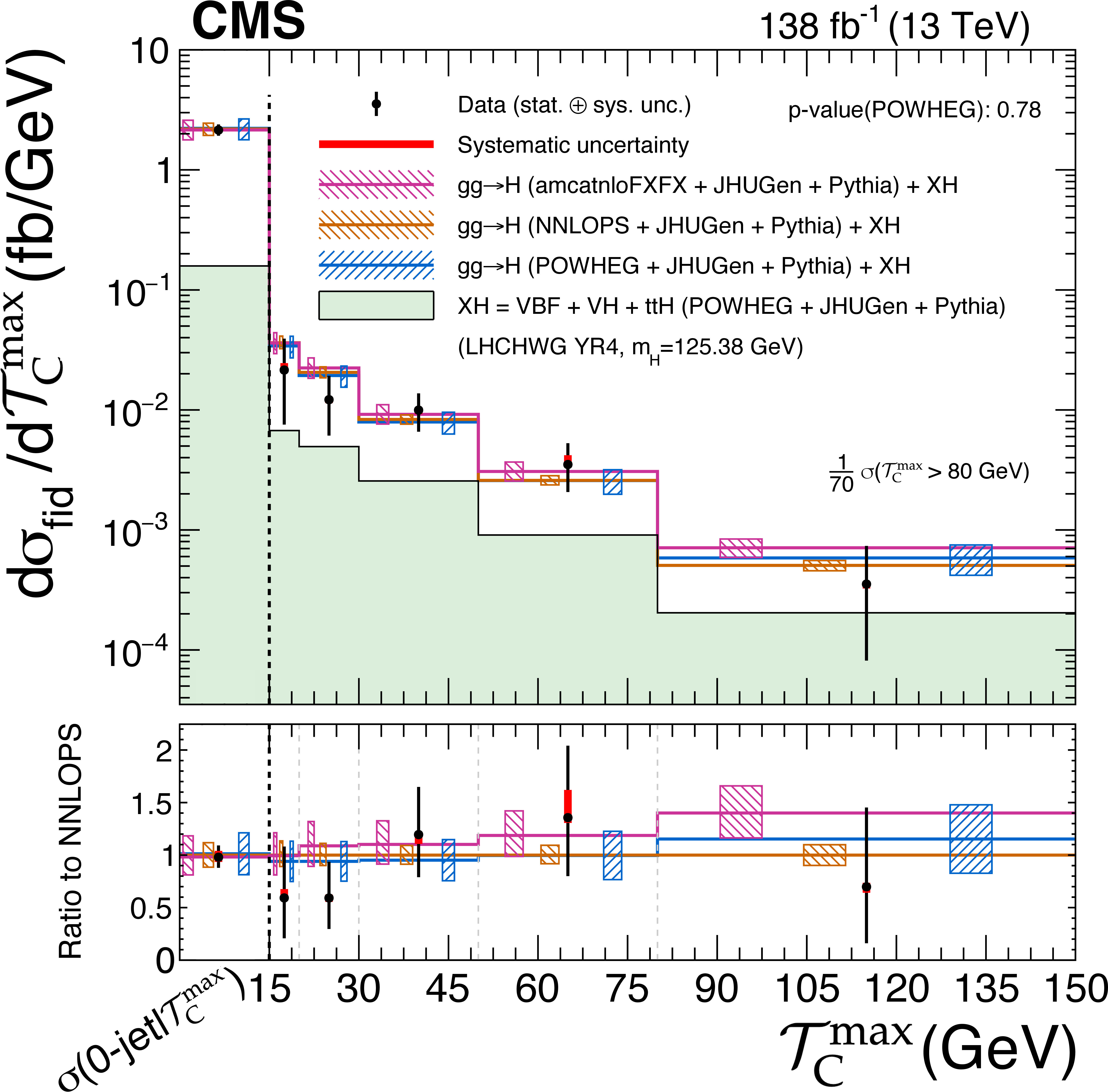
Figure 10-a:
Differential cross sections as functions of the rapidity-weighed jet veto $ \mathcal{T}_{\text{C}}^{\text{max}} $. The fiducial cross section in the last bin is measured for events with $ \mathcal{T}_{\text{C}}^{\text{max}} > $ 80 GeV and normalized to a bin width of 70 GeV. The first bin comprises all events in the 0-jet phase space region redefined as a function of $ \mathcal{T}_{\text{C}}^{\text{max}} $, i.e.,, events with less than one jet, for which $ \mathcal{T}_{\text{C}}^{\text{max}} $ is undefined, and events with $ \mathcal{T}_{\text{C}}^{\text{max}} < $ 15 GeV. The acceptance and theoretical uncertainties in the differential bins are calculated using the ggH predictions from the POWHEG generator (blue) normalized to $ \mathrm{N^3LO} $. The subdominant component of the signal (VBF+VH+ttH) is denoted as XH and is fixed to the SM prediction. The measured cross sections are also compared with the ggH predictions from NNLOPS (orange) and MadGraph-5_aMC@NLO (pink). The hatched areas correspond to the systematic uncertainties in the theoretical predictions. Black points represent the measured fiducial cross sections in each bin, black error bars the total uncertainty in each measurement, red boxes the systematic uncertainties. The lower panel displays the ratios of the measured cross sections and of the predictions from POWHEG and MadGraph-5_aMC@NLO to the NNLOPS theoretical predictions. |

png pdf |
Figure 10-b:
Differential cross sections as functions of the rapidity-weighed jet veto $ \mathcal{T}_{\text{B}}^{\text{max}} $. The fiducial cross section in the last bin is measured for events with $ \mathcal{T}_{\text{B}}^{\text{max}} > $ 150 GeV and normalized to a bin width of 150 GeV. The first bin comprises all events in the 0-jet phase space region redefined as a function of $ \mathcal{T}_{\text{B}}^{\text{max}} $, i.e.,, events with less than one jet, for which $ \mathcal{T}_{\text{B}}^{\text{max}} $ is undefined, and events with $ \mathcal{T}_{\text{B}}^{\text{max}} < $ 30 GeV. The acceptance and theoretical uncertainties in the differential bins are calculated using the ggH predictions from the POWHEG generator (blue) normalized to $ \mathrm{N^3LO} $. The subdominant component of the signal (VBF+VH+ttH) is denoted as XH and is fixed to the SM prediction. The measured cross sections are also compared with the ggH predictions from NNLOPS (orange) and MadGraph-5_aMC@NLO (pink). The hatched areas correspond to the systematic uncertainties in the theoretical predictions. Black points represent the measured fiducial cross sections in each bin, black error bars the total uncertainty in each measurement, red boxes the systematic uncertainties. The lower panel displays the ratios of the measured cross sections and of the predictions from POWHEG and MadGraph-5_aMC@NLO to the NNLOPS theoretical predictions. |

png pdf |
Figure 11:
Differential cross sections as functions of the invariant mass of the leading dilepton pair $ m_{\mathrm{Z}_{1}} $ in the 4$ \ell $ (upper) and in the same-flavor (lower left) and different-flavor (lower right) final states. The acceptance and theoretical uncertainties in the differential bins are calculated using the ggH predictions from the POWHEG generator (blue) normalized to $ \mathrm{N^3LO} $. The subdominant component of the signal (VBF+VH+ttH) is denoted as XH and is fixed to the SM prediction. The measured cross sections are also compared with the ggH predictions from NNLOPS (orange) and MadGraph-5_aMC@NLO (pink). The hatched areas correspond to the systematic uncertainties in the theoretical predictions. Black points represent the measured fiducial cross sections in each bin, black error bars the total uncertainty in each measurement, red boxes the systematic uncertainties. The lower panels display the ratios of the measured cross sections and of the predictions from POWHEG and MadGraph-5_aMC@NLO to the NNLOPS theoretical predictions. |

png pdf |
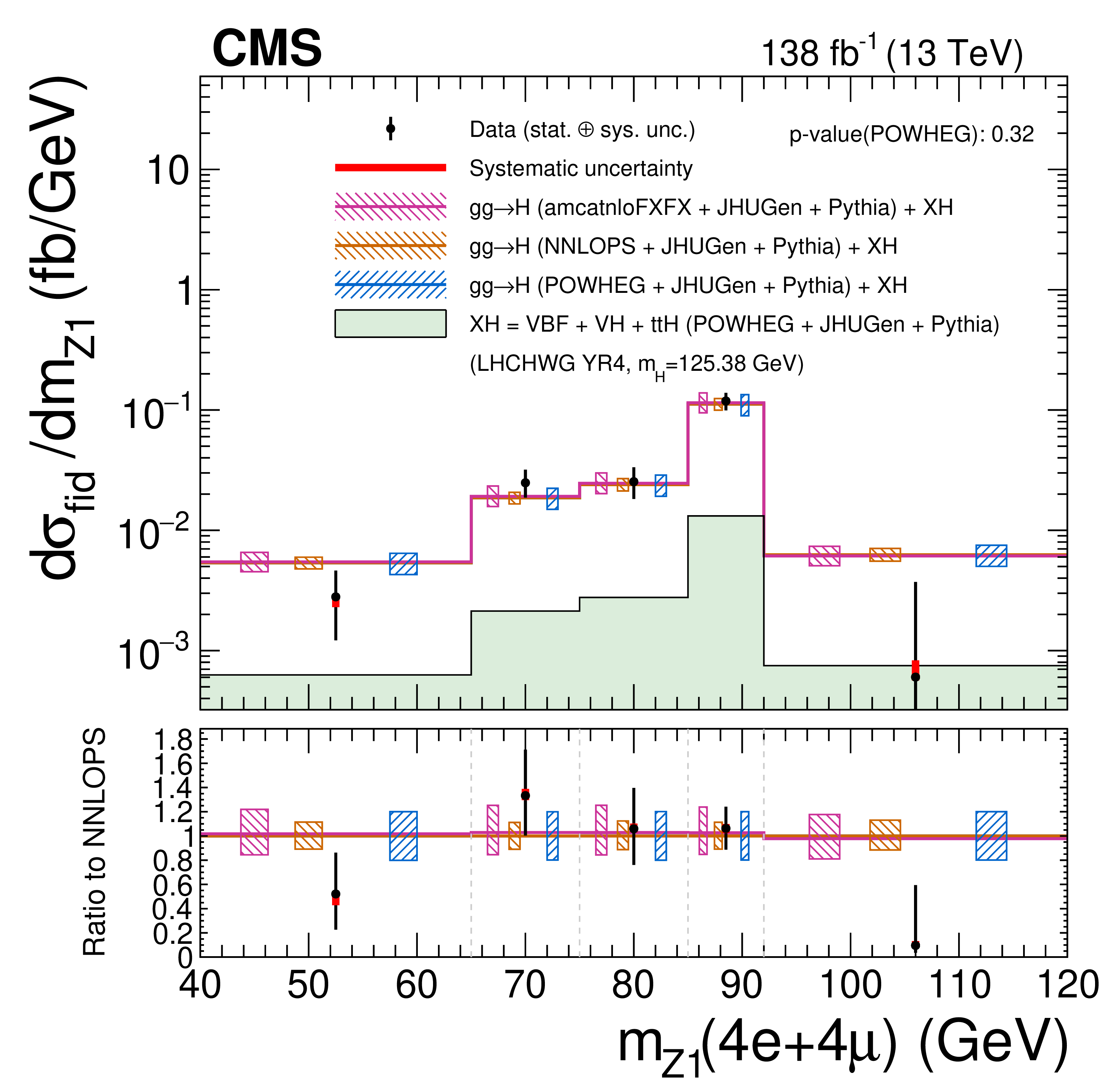
Figure 11-a:
Differential cross sections as functions of the invariant mass of the leading dilepton pair $ m_{\mathrm{Z}_{1}} $ in the 4$ \ell $ final states. The acceptance and theoretical uncertainties in the differential bins are calculated using the ggH predictions from the POWHEG generator (blue) normalized to $ \mathrm{N^3LO} $. The subdominant component of the signal (VBF+VH+ttH) is denoted as XH and is fixed to the SM prediction. The measured cross sections are also compared with the ggH predictions from NNLOPS (orange) and MadGraph-5_aMC@NLO (pink). The hatched areas correspond to the systematic uncertainties in the theoretical predictions. Black points represent the measured fiducial cross sections in each bin, black error bars the total uncertainty in each measurement, red boxes the systematic uncertainties. The lower panel displays the ratios of the measured cross sections and of the predictions from POWHEG and MadGraph-5_aMC@NLO to the NNLOPS theoretical predictions. |
png pdf |
Figure 11-b:
Differential cross sections as functions of the invariant mass of the leading dilepton pair $ m_{\mathrm{Z}_{1}} $ in the same-flavor final states. The acceptance and theoretical uncertainties in the differential bins are calculated using the ggH predictions from the POWHEG generator (blue) normalized to $ \mathrm{N^3LO} $. The subdominant component of the signal (VBF+VH+ttH) is denoted as XH and is fixed to the SM prediction. The measured cross sections are also compared with the ggH predictions from NNLOPS (orange) and MadGraph-5_aMC@NLO (pink). The hatched areas correspond to the systematic uncertainties in the theoretical predictions. Black points represent the measured fiducial cross sections in each bin, black error bars the total uncertainty in each measurement, red boxes the systematic uncertainties. The lower panel displays the ratios of the measured cross sections and of the predictions from POWHEG and MadGraph-5_aMC@NLO to the NNLOPS theoretical predictions. |

png pdf |
Figure 11-c:
Differential cross sections as functions of the invariant mass of the leading dilepton pair $ m_{\mathrm{Z}_{1}} $ in the different-flavor final states. The acceptance and theoretical uncertainties in the differential bins are calculated using the ggH predictions from the POWHEG generator (blue) normalized to $ \mathrm{N^3LO} $. The subdominant component of the signal (VBF+VH+ttH) is denoted as XH and is fixed to the SM prediction. The measured cross sections are also compared with the ggH predictions from NNLOPS (orange) and MadGraph-5_aMC@NLO (pink). The hatched areas correspond to the systematic uncertainties in the theoretical predictions. Black points represent the measured fiducial cross sections in each bin, black error bars the total uncertainty in each measurement, red boxes the systematic uncertainties. The lower panel displays the ratios of the measured cross sections and of the predictions from POWHEG and MadGraph-5_aMC@NLO to the NNLOPS theoretical predictions. |

png pdf |
Figure 12:
Differential cross sections as functions of the invariant mass of the subleading dilepton pair $ m_{\mathrm{Z}_{2}} $ in the 4$ \ell $ (upper) and in the same-flavor (lower left) and different-flavor (lower right) final states. The acceptance and theoretical uncertainties in the differential bins are calculated using the ggH predictions from the POWHEG generator (blue) normalized to $ \mathrm{N^3LO} $. The subdominant component of the signal (VBF+VH+ttH) is denoted as XH and is fixed to the SM prediction. The measured cross sections are also compared with the ggH predictions from NNLOPS (orange) and MadGraph-5_aMC@NLO (pink). The hatched areas correspond to the systematic uncertainties in the theoretical predictions. Black points represent the measured fiducial cross sections in each bin, black error bars the total uncertainty in each measurement, red boxes the systematic uncertainties. The lower panels display the ratios of the measured cross sections and of the predictions from POWHEG and MadGraph-5_aMC@NLO to the NNLOPS theoretical predictions. |
png pdf |
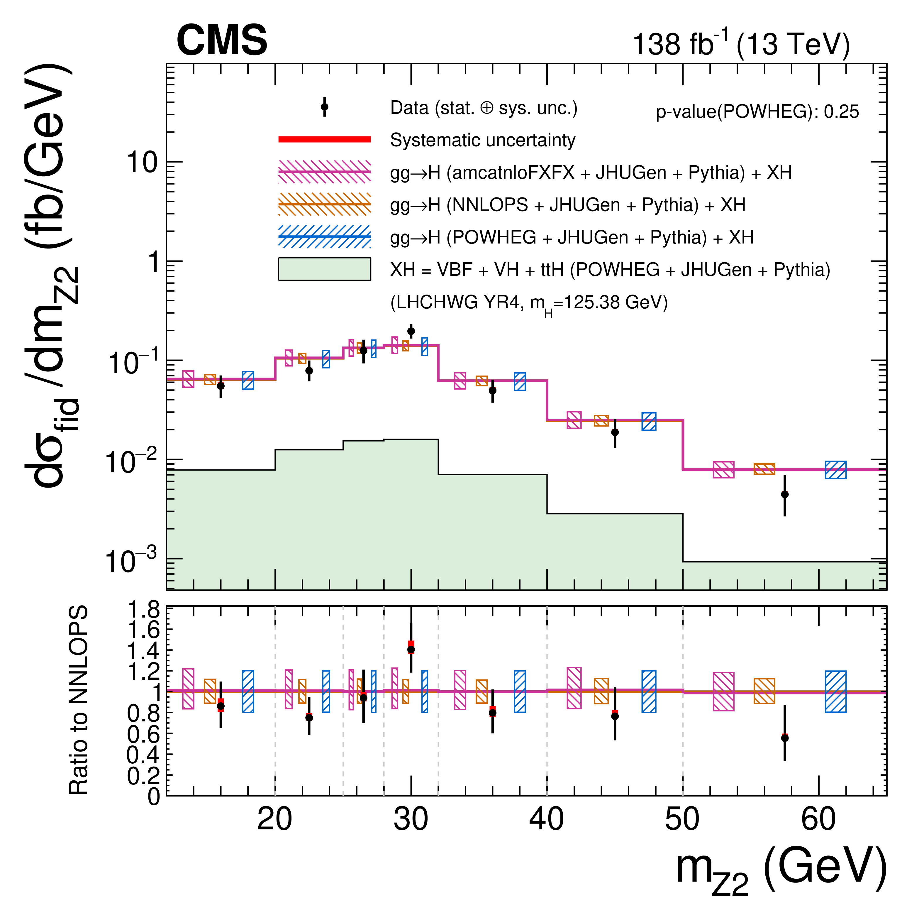
Figure 12-a:
Differential cross sections as functions of the invariant mass of the subleading dilepton pair $ m_{\mathrm{Z}_{2}} $ in the 4$ \ell $ final states. The acceptance and theoretical uncertainties in the differential bins are calculated using the ggH predictions from the POWHEG generator (blue) normalized to $ \mathrm{N^3LO} $. The subdominant component of the signal (VBF+VH+ttH) is denoted as XH and is fixed to the SM prediction. The measured cross sections are also compared with the ggH predictions from NNLOPS (orange) and MadGraph-5_aMC@NLO (pink). The hatched areas correspond to the systematic uncertainties in the theoretical predictions. Black points represent the measured fiducial cross sections in each bin, black error bars the total uncertainty in each measurement, red boxes the systematic uncertainties. The lower panel displays the ratios of the measured cross sections and of the predictions from POWHEG and MadGraph-5_aMC@NLO to the NNLOPS theoretical predictions. |

png pdf |
Figure 12-b:
Differential cross sections as functions of the invariant mass of the subleading dilepton pair $ m_{\mathrm{Z}_{2}} $ in the same-flavor final states. The acceptance and theoretical uncertainties in the differential bins are calculated using the ggH predictions from the POWHEG generator (blue) normalized to $ \mathrm{N^3LO} $. The subdominant component of the signal (VBF+VH+ttH) is denoted as XH and is fixed to the SM prediction. The measured cross sections are also compared with the ggH predictions from NNLOPS (orange) and MadGraph-5_aMC@NLO (pink). The hatched areas correspond to the systematic uncertainties in the theoretical predictions. Black points represent the measured fiducial cross sections in each bin, black error bars the total uncertainty in each measurement, red boxes the systematic uncertainties. The lower panel displays the ratios of the measured cross sections and of the predictions from POWHEG and MadGraph-5_aMC@NLO to the NNLOPS theoretical predictions. |

png pdf |
Figure 12-c:
Differential cross sections as functions of the invariant mass of the subleading dilepton pair $ m_{\mathrm{Z}_{2}} $ in the different-flavor final states. The acceptance and theoretical uncertainties in the differential bins are calculated using the ggH predictions from the POWHEG generator (blue) normalized to $ \mathrm{N^3LO} $. The subdominant component of the signal (VBF+VH+ttH) is denoted as XH and is fixed to the SM prediction. The measured cross sections are also compared with the ggH predictions from NNLOPS (orange) and MadGraph-5_aMC@NLO (pink). The hatched areas correspond to the systematic uncertainties in the theoretical predictions. Black points represent the measured fiducial cross sections in each bin, black error bars the total uncertainty in each measurement, red boxes the systematic uncertainties. The lower panel displays the ratios of the measured cross sections and of the predictions from POWHEG and MadGraph-5_aMC@NLO to the NNLOPS theoretical predictions. |

png pdf |
Figure 13:
Differential cross sections as functions of $ \cos \theta^* $ in the 4$ \ell $ (upper) and in the same-flavor (lower left) and different-flavor (lower right) final states. The acceptance and theoretical uncertainties in the differential bins are calculated using the ggH predictions from the POWHEG generator (blue) normalized to $ \mathrm{N^3LO} $. The subdominant component of the signal (VBF+VH+ttH) is denoted as XH and is fixed to the SM prediction. The measured cross sections are also compared with the ggH predictions from NNLOPS (orange) and MadGraph-5_aMC@NLO (pink). The hatched areas correspond to the systematic uncertainties in the theoretical predictions. Black points represent the measured fiducial cross sections in each bin, black error bars the total uncertainty in each measurement, red boxes the systematic uncertainties. The lower panels display the ratios of the measured cross sections and of the predictions from POWHEG and MadGraph-5_aMC@NLO to the NNLOPS theoretical predictions. |

png pdf |
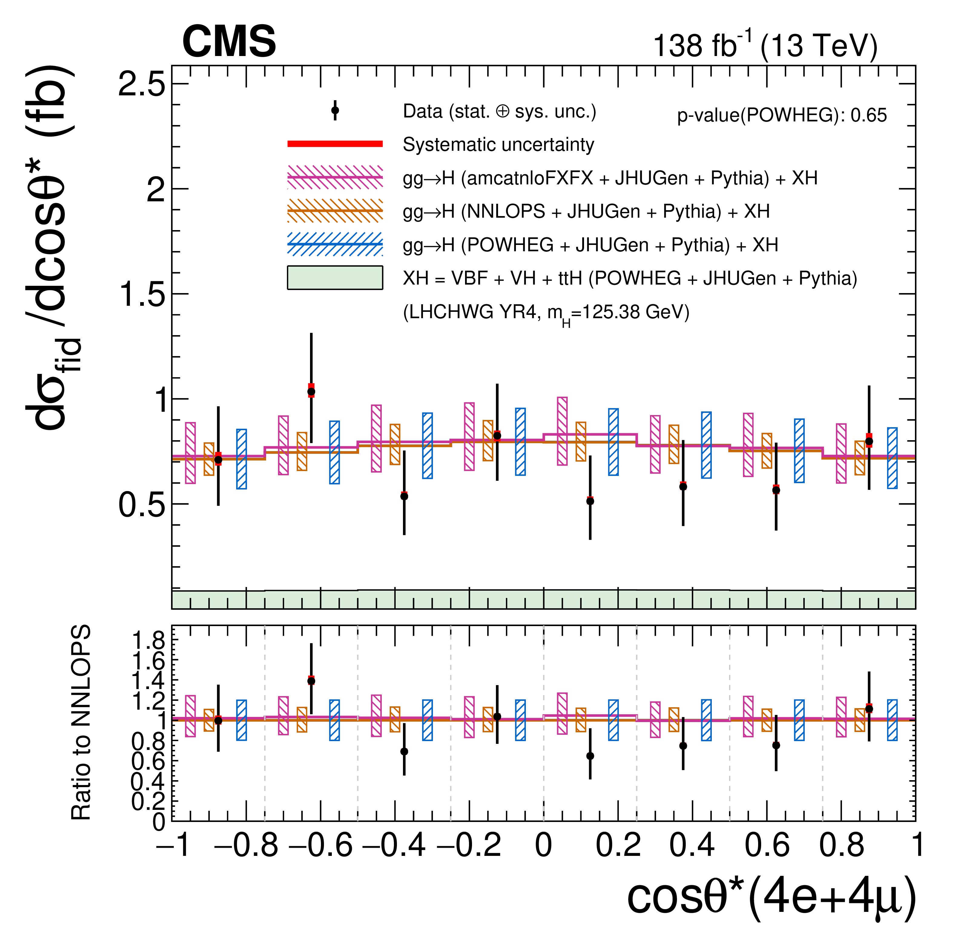
Figure 13-a:
Differential cross sections as functions of $ \cos \theta^* $ in the 4$ \ell $ final states. The acceptance and theoretical uncertainties in the differential bins are calculated using the ggH predictions from the POWHEG generator (blue) normalized to $ \mathrm{N^3LO} $. The subdominant component of the signal (VBF+VH+ttH) is denoted as XH and is fixed to the SM prediction. The measured cross sections are also compared with the ggH predictions from NNLOPS (orange) and MadGraph-5_aMC@NLO (pink). The hatched areas correspond to the systematic uncertainties in the theoretical predictions. Black points represent the measured fiducial cross sections in each bin, black error bars the total uncertainty in each measurement, red boxes the systematic uncertainties. The lower panel displays the ratios of the measured cross sections and of the predictions from POWHEG and MadGraph-5_aMC@NLO to the NNLOPS theoretical predictions. |
png pdf |
Figure 13-b:
Differential cross sections as functions of $ \cos \theta^* $ in the same-flavor final states. The acceptance and theoretical uncertainties in the differential bins are calculated using the ggH predictions from the POWHEG generator (blue) normalized to $ \mathrm{N^3LO} $. The subdominant component of the signal (VBF+VH+ttH) is denoted as XH and is fixed to the SM prediction. The measured cross sections are also compared with the ggH predictions from NNLOPS (orange) and MadGraph-5_aMC@NLO (pink). The hatched areas correspond to the systematic uncertainties in the theoretical predictions. Black points represent the measured fiducial cross sections in each bin, black error bars the total uncertainty in each measurement, red boxes the systematic uncertainties. The lower panel displays the ratios of the measured cross sections and of the predictions from POWHEG and MadGraph-5_aMC@NLO to the NNLOPS theoretical predictions. |
png pdf |
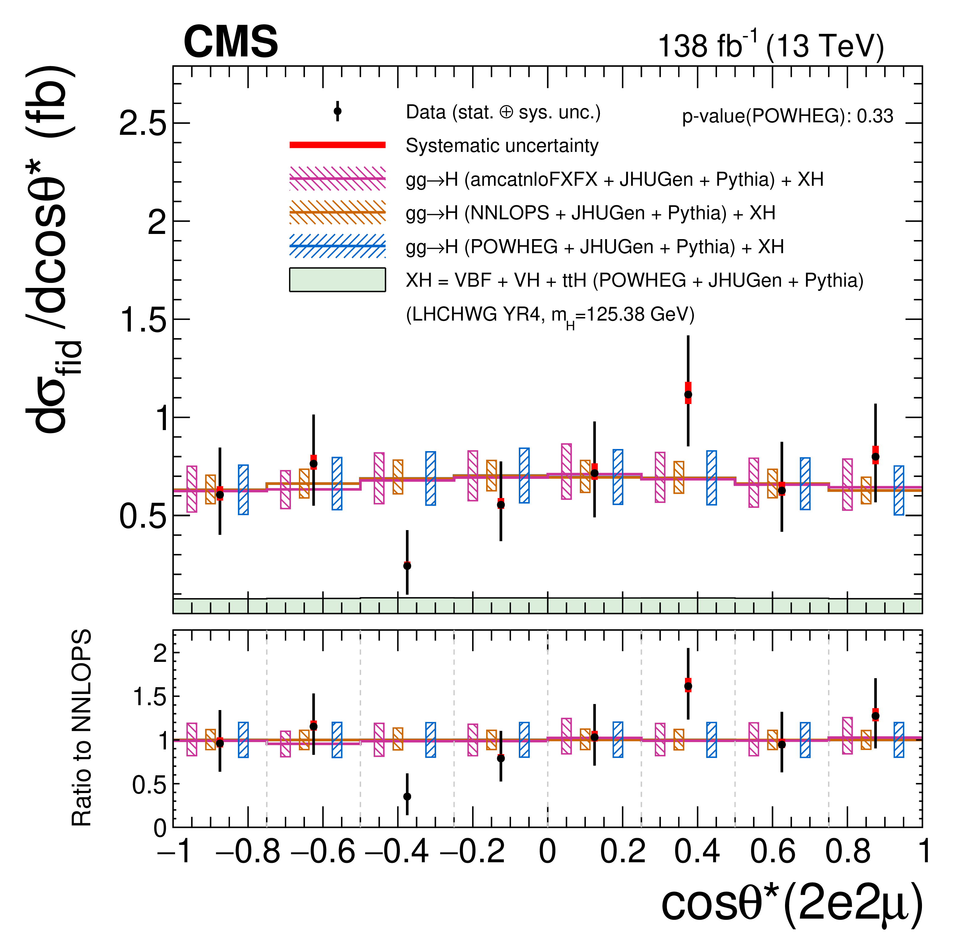
Figure 13-c:
Differential cross sections as functions of $ \cos \theta^* $ in the different-flavor final states. The acceptance and theoretical uncertainties in the differential bins are calculated using the ggH predictions from the POWHEG generator (blue) normalized to $ \mathrm{N^3LO} $. The subdominant component of the signal (VBF+VH+ttH) is denoted as XH and is fixed to the SM prediction. The measured cross sections are also compared with the ggH predictions from NNLOPS (orange) and MadGraph-5_aMC@NLO (pink). The hatched areas correspond to the systematic uncertainties in the theoretical predictions. Black points represent the measured fiducial cross sections in each bin, black error bars the total uncertainty in each measurement, red boxes the systematic uncertainties. The lower panel displays the ratios of the measured cross sections and of the predictions from POWHEG and MadGraph-5_aMC@NLO to the NNLOPS theoretical predictions. |
png pdf |
Figure 14:
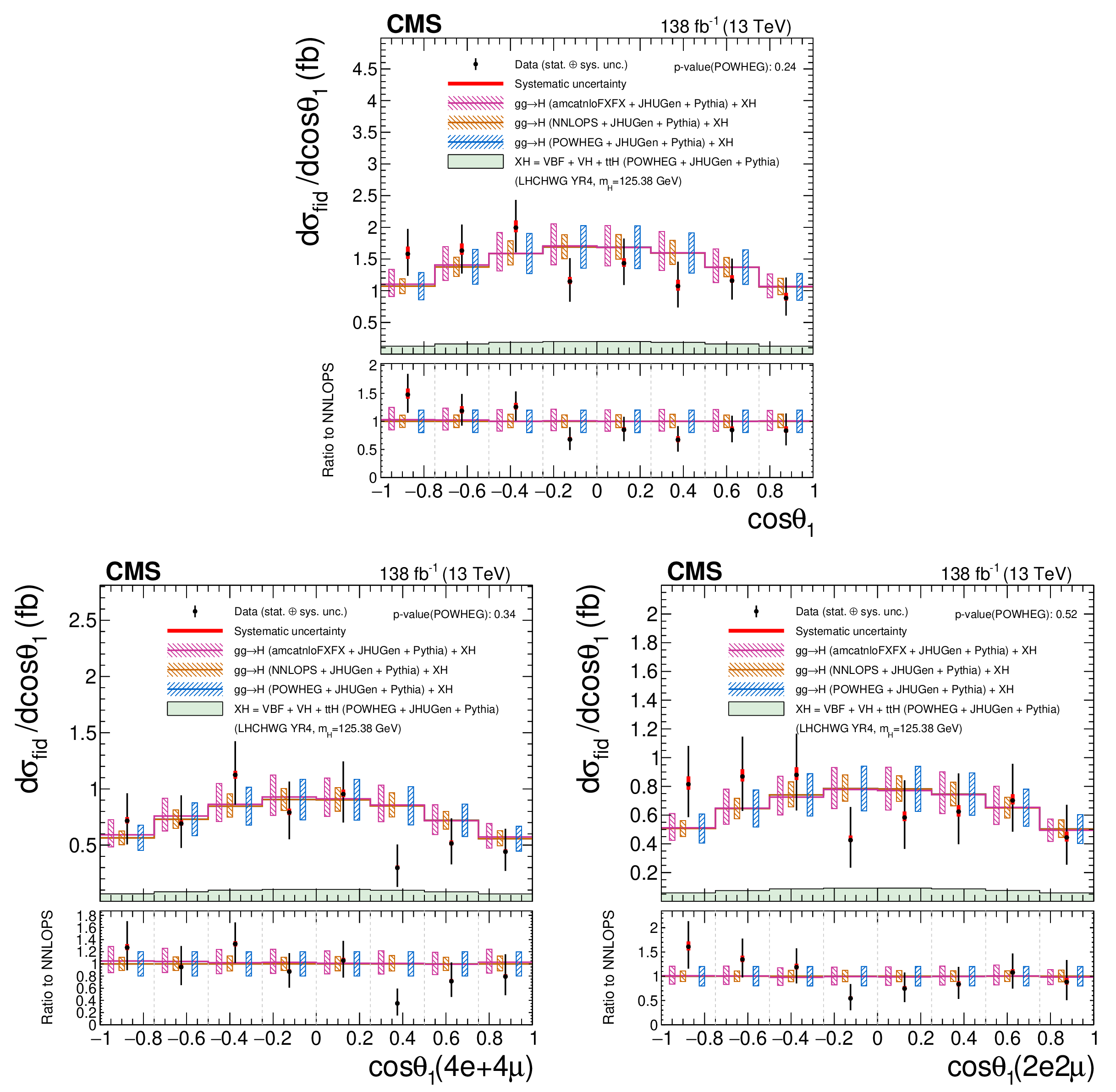
Differential cross sections as functions of $ \cos \theta_\text{1} $ in the 4$ \ell $ (upper) and in the same-flavor (lower left) and different-flavor (lower right) final states. The acceptance and theoretical uncertainties in the differential bins are calculated using the ggH predictions from the POWHEG generator (blue) normalized to $ \mathrm{N^3LO} $. The subdominant component of the signal (VBF+VH+ttH) is denoted as XH and is fixed to the SM prediction. The measured cross sections are also compared with the ggH predictions from NNLOPS (orange) and MadGraph-5_aMC@NLO (pink). The hatched areas correspond to the systematic uncertainties in the theoretical predictions. Black points represent the measured fiducial cross sections in each bin, black error bars the total uncertainty in each measurement, red boxes the systematic uncertainties. The lower panels display the ratios of the measured cross sections and of the predictions from POWHEG and MadGraph-5_aMC@NLO to the NNLOPS theoretical predictions. |
png pdf |
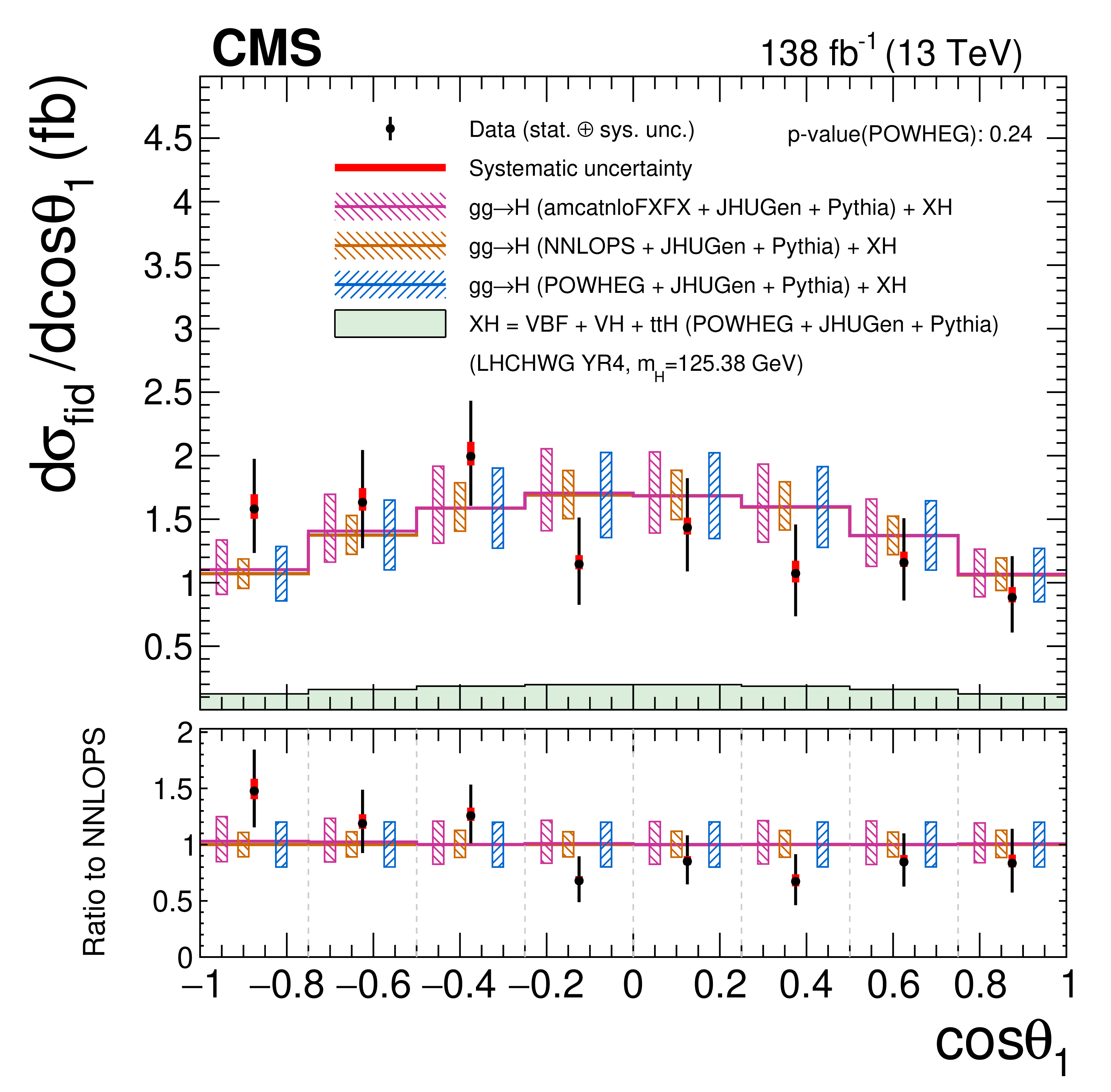
Figure 14-a:
Differential cross sections as functions of $ \cos \theta_\text{1} $ in the 4$ \ell $ final states. The acceptance and theoretical uncertainties in the differential bins are calculated using the ggH predictions from the POWHEG generator (blue) normalized to $ \mathrm{N^3LO} $. The subdominant component of the signal (VBF+VH+ttH) is denoted as XH and is fixed to the SM prediction. The measured cross sections are also compared with the ggH predictions from NNLOPS (orange) and MadGraph-5_aMC@NLO (pink). The hatched areas correspond to the systematic uncertainties in the theoretical predictions. Black points represent the measured fiducial cross sections in each bin, black error bars the total uncertainty in each measurement, red boxes the systematic uncertainties. The lower panel displays the ratios of the measured cross sections and of the predictions from POWHEG and MadGraph-5_aMC@NLO to the NNLOPS theoretical predictions. |

png pdf |
Figure 14-b:
Differential cross sections as functions of $ \cos \theta_\text{1} $ in the same-flavor final states. The acceptance and theoretical uncertainties in the differential bins are calculated using the ggH predictions from the POWHEG generator (blue) normalized to $ \mathrm{N^3LO} $. The subdominant component of the signal (VBF+VH+ttH) is denoted as XH and is fixed to the SM prediction. The measured cross sections are also compared with the ggH predictions from NNLOPS (orange) and MadGraph-5_aMC@NLO (pink). The hatched areas correspond to the systematic uncertainties in the theoretical predictions. Black points represent the measured fiducial cross sections in each bin, black error bars the total uncertainty in each measurement, red boxes the systematic uncertainties. The lower panel displays the ratios of the measured cross sections and of the predictions from POWHEG and MadGraph-5_aMC@NLO to the NNLOPS theoretical predictions. |
png pdf |
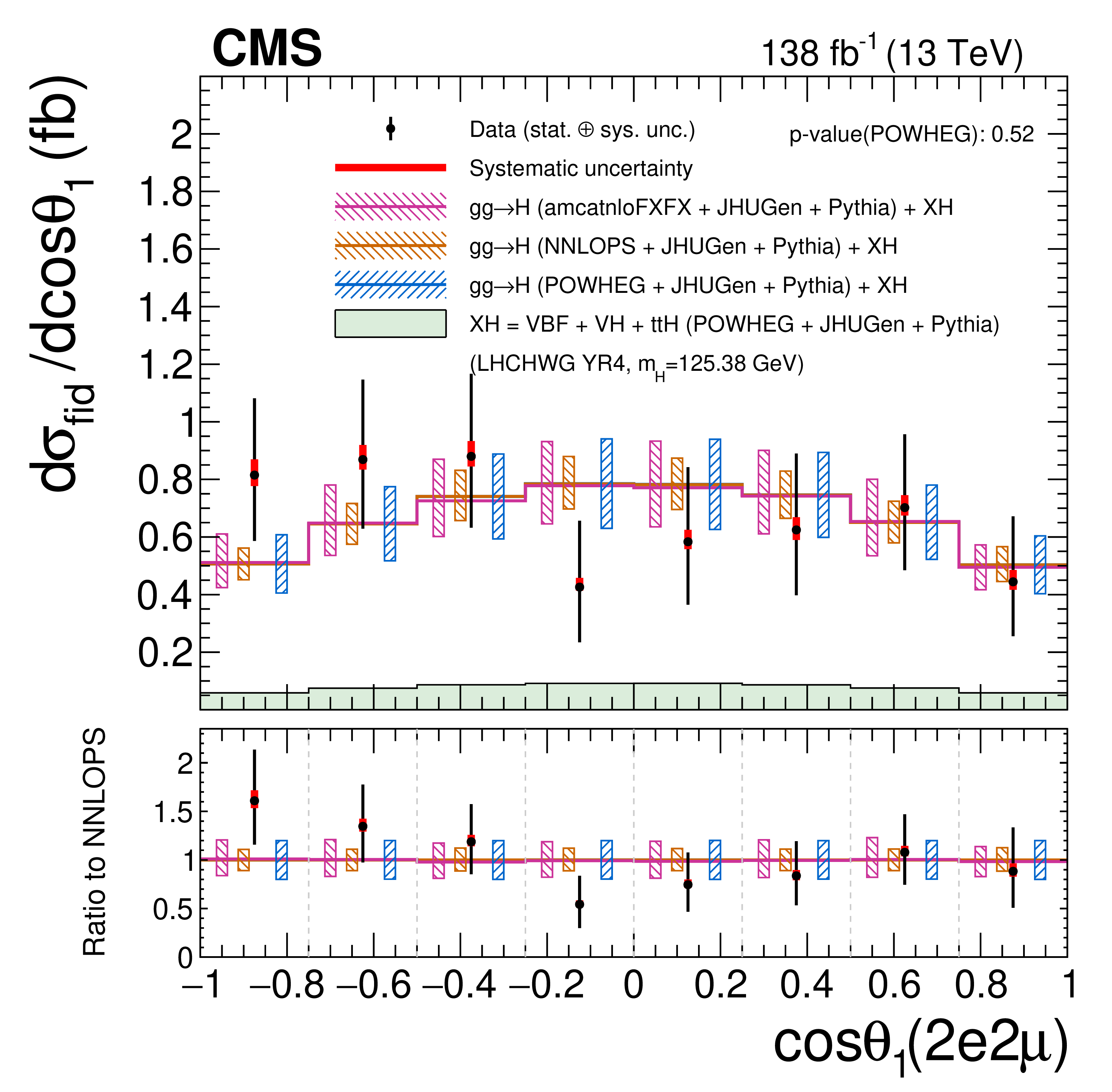
Figure 14-c:
Differential cross sections as functions of $ \cos \theta_\text{1} $ in the different-flavor final states. The acceptance and theoretical uncertainties in the differential bins are calculated using the ggH predictions from the POWHEG generator (blue) normalized to $ \mathrm{N^3LO} $. The subdominant component of the signal (VBF+VH+ttH) is denoted as XH and is fixed to the SM prediction. The measured cross sections are also compared with the ggH predictions from NNLOPS (orange) and MadGraph-5_aMC@NLO (pink). The hatched areas correspond to the systematic uncertainties in the theoretical predictions. Black points represent the measured fiducial cross sections in each bin, black error bars the total uncertainty in each measurement, red boxes the systematic uncertainties. The lower panel displays the ratios of the measured cross sections and of the predictions from POWHEG and MadGraph-5_aMC@NLO to the NNLOPS theoretical predictions. |
png pdf |
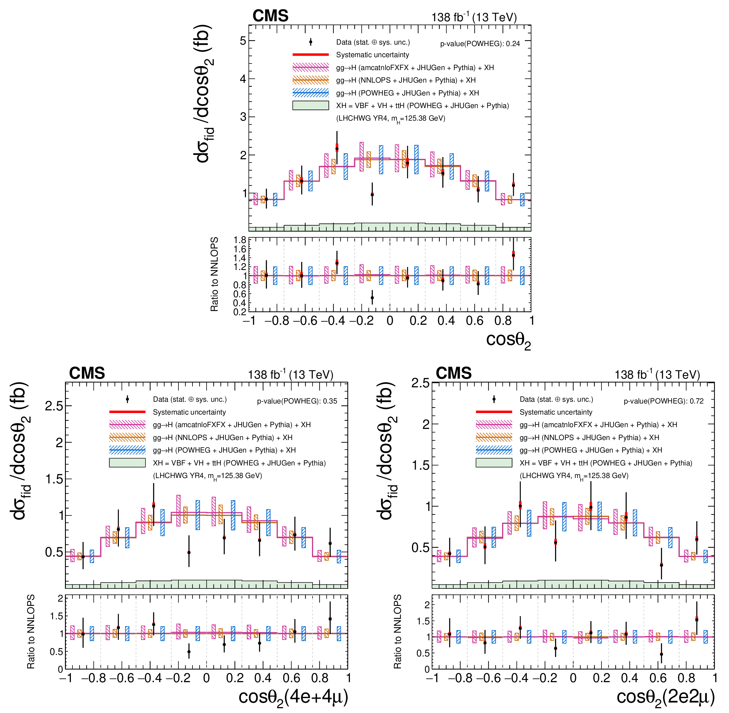
Figure 15:
Differential cross sections as functions of $ \cos \theta_\text{2} $ in the 4$ \ell $ (upper) and in the same-flavor (lower left) and different-flavor (lower right) final states. The acceptance and theoretical uncertainties in the differential bins are calculated using the ggH predictions from the POWHEG generator (blue) normalized to $ \mathrm{N^3LO} $. The subdominant component of the signal (VBF+VH+ttH) is denoted as XH and is fixed to the SM prediction. The measured cross sections are also compared with the ggH predictions from NNLOPS (orange) and MadGraph-5_aMC@NLO (pink). The hatched areas correspond to the systematic uncertainties in the theoretical predictions. Black points represent the measured fiducial cross sections in each bin, black error bars the total uncertainty in each measurement, red boxes the systematic uncertainties. The lower panels display the ratios of the measured cross sections and of the predictions from POWHEG and MadGraph-5_aMC@NLO to the NNLOPS theoretical predictions. |

png pdf |
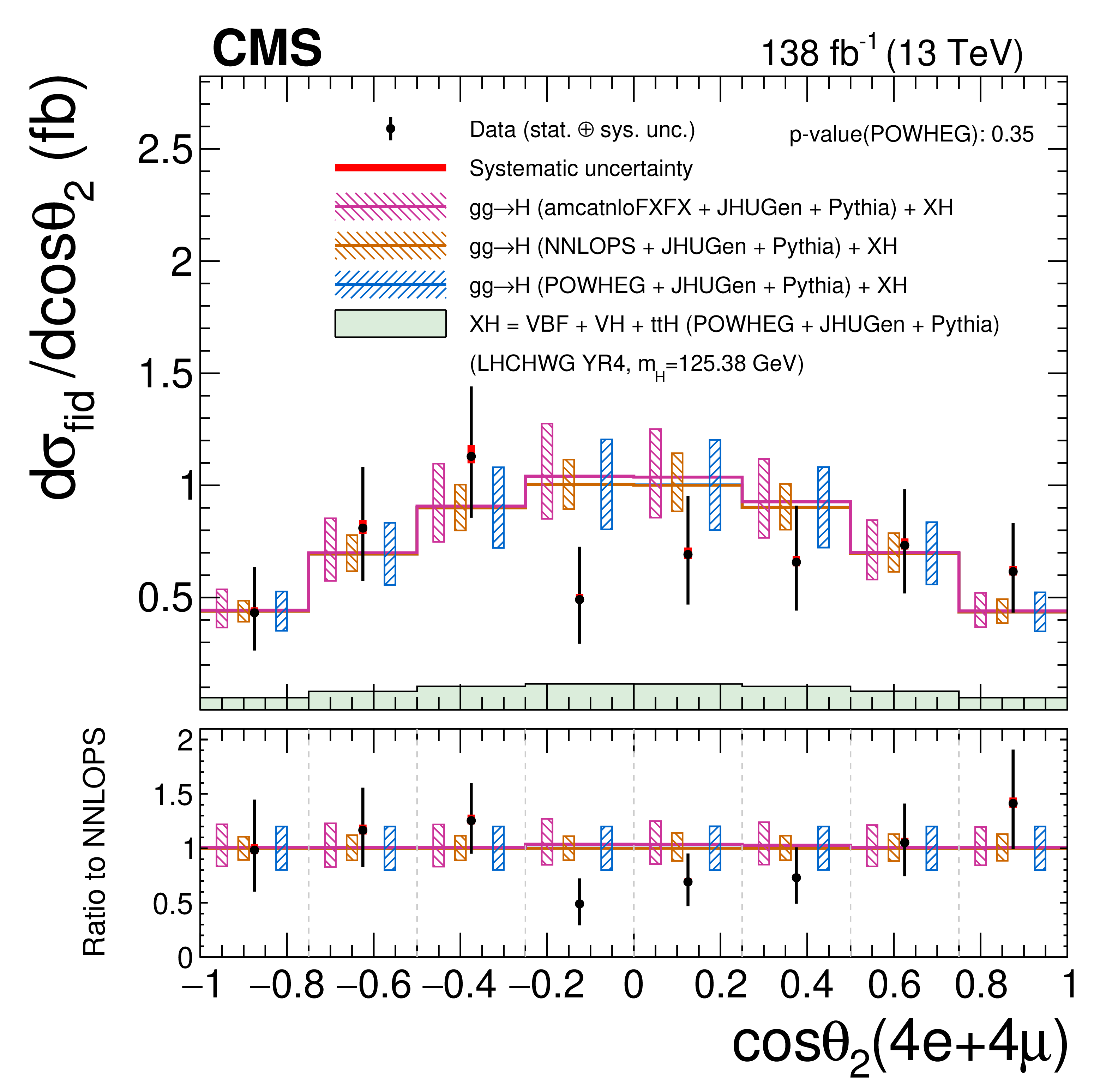
Figure 15-a:
Differential cross sections as functions of $ \cos \theta_\text{2} $ in the 4$ \ell $ final states. The acceptance and theoretical uncertainties in the differential bins are calculated using the ggH predictions from the POWHEG generator (blue) normalized to $ \mathrm{N^3LO} $. The subdominant component of the signal (VBF+VH+ttH) is denoted as XH and is fixed to the SM prediction. The measured cross sections are also compared with the ggH predictions from NNLOPS (orange) and MadGraph-5_aMC@NLO (pink). The hatched areas correspond to the systematic uncertainties in the theoretical predictions. Black points represent the measured fiducial cross sections in each bin, black error bars the total uncertainty in each measurement, red boxes the systematic uncertainties. The lower panel displays the ratios of the measured cross sections and of the predictions from POWHEG and MadGraph-5_aMC@NLO to the NNLOPS theoretical predictions. |
png pdf |
Figure 15-b:
Differential cross sections as functions of $ \cos \theta_\text{2} $ in the same-flavor final states. The acceptance and theoretical uncertainties in the differential bins are calculated using the ggH predictions from the POWHEG generator (blue) normalized to $ \mathrm{N^3LO} $. The subdominant component of the signal (VBF+VH+ttH) is denoted as XH and is fixed to the SM prediction. The measured cross sections are also compared with the ggH predictions from NNLOPS (orange) and MadGraph-5_aMC@NLO (pink). The hatched areas correspond to the systematic uncertainties in the theoretical predictions. Black points represent the measured fiducial cross sections in each bin, black error bars the total uncertainty in each measurement, red boxes the systematic uncertainties. The lower panel displays the ratios of the measured cross sections and of the predictions from POWHEG and MadGraph-5_aMC@NLO to the NNLOPS theoretical predictions. |

png pdf |
Figure 15-c:
Differential cross sections as functions of $ \cos \theta_\text{2} $ in the different-flavor final states. The acceptance and theoretical uncertainties in the differential bins are calculated using the ggH predictions from the POWHEG generator (blue) normalized to $ \mathrm{N^3LO} $. The subdominant component of the signal (VBF+VH+ttH) is denoted as XH and is fixed to the SM prediction. The measured cross sections are also compared with the ggH predictions from NNLOPS (orange) and MadGraph-5_aMC@NLO (pink). The hatched areas correspond to the systematic uncertainties in the theoretical predictions. Black points represent the measured fiducial cross sections in each bin, black error bars the total uncertainty in each measurement, red boxes the systematic uncertainties. The lower panel displays the ratios of the measured cross sections and of the predictions from POWHEG and MadGraph-5_aMC@NLO to the NNLOPS theoretical predictions. |
png pdf |
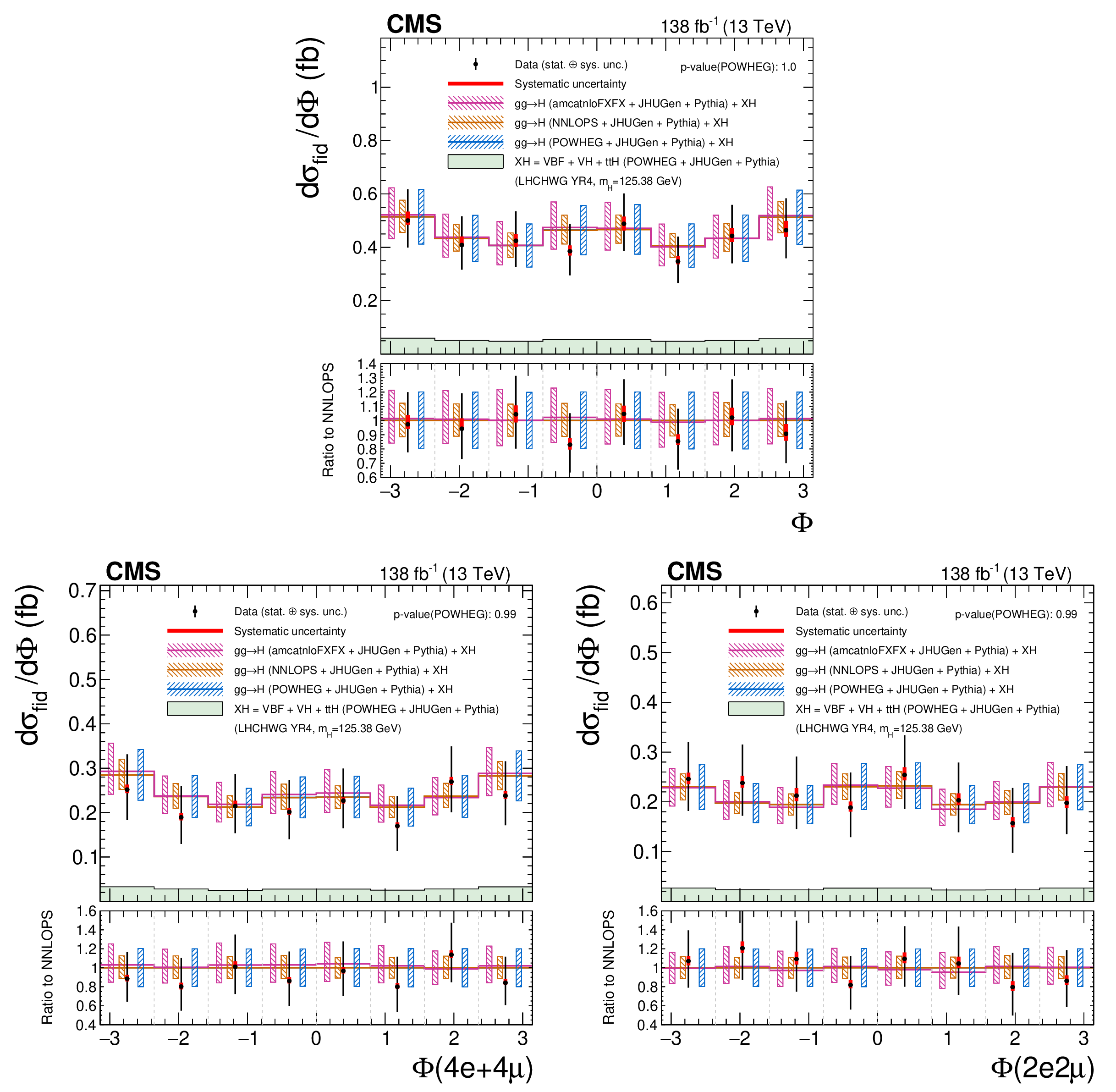
Figure 16:
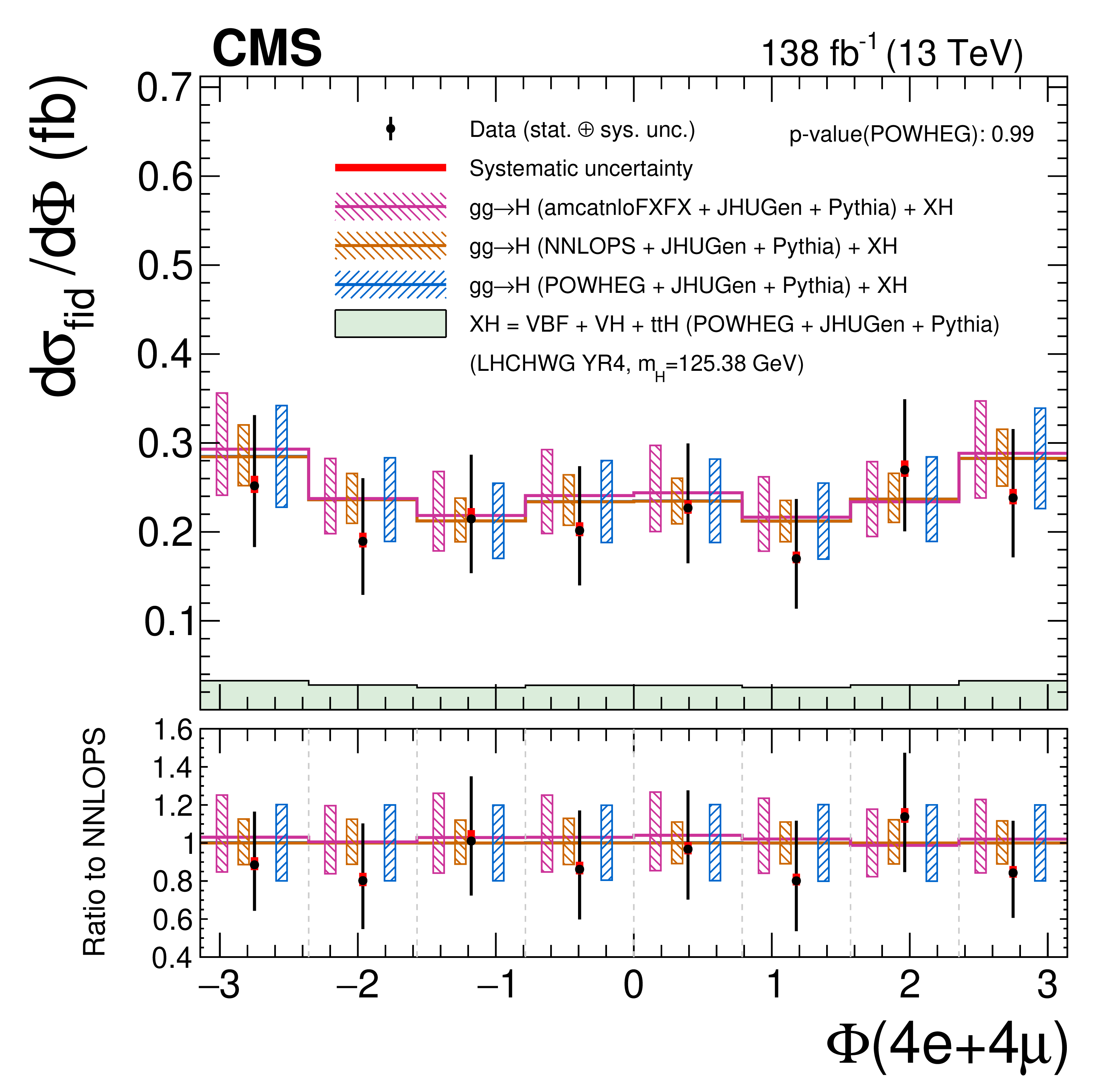
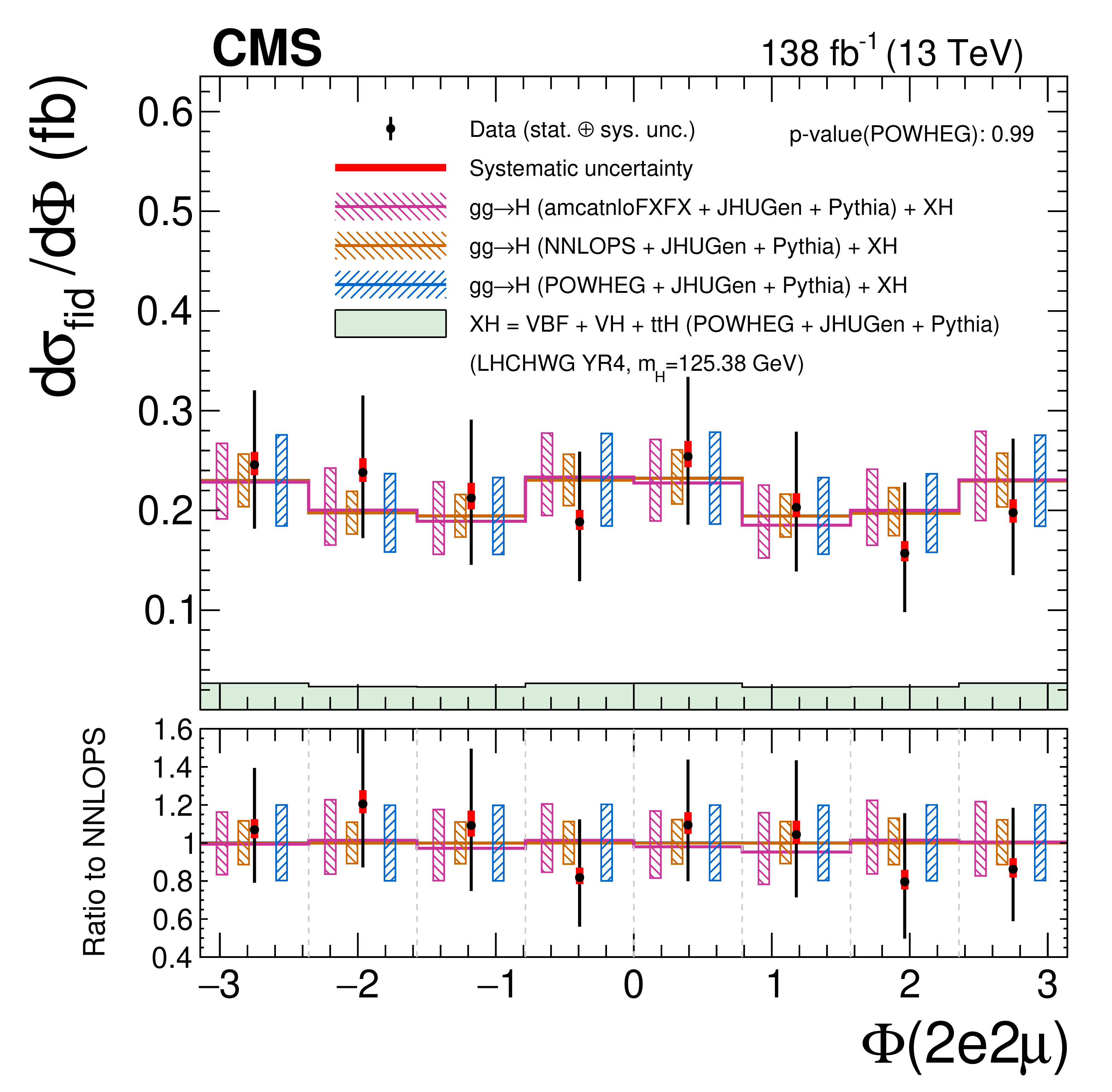
Differential cross sections as functions of the $ \Phi $ angle in the 4$ \ell $ (upper) and in the same-flavor (lower left) and different-flavor (lower right) final states. The acceptance and theoretical uncertainties in the differential bins are calculated using the ggH predictions from the POWHEG generator (blue) normalized to $ \mathrm{N^3LO} $. The subdominant component of the signal (VBF+VH+ttH) is denoted as XH and is fixed to the SM prediction. The measured cross sections are also compared with the ggH predictions from NNLOPS (orange) and MadGraph-5_aMC@NLO (pink). The hatched areas correspond to the systematic uncertainties in the theoretical predictions. Black points represent the measured fiducial cross sections in each bin, black error bars the total uncertainty in each measurement, red boxes the systematic uncertainties. The lower panels display the ratios of the measured cross sections and of the predictions from POWHEG and MadGraph-5_aMC@NLO to the NNLOPS theoretical predictions. |
png pdf |
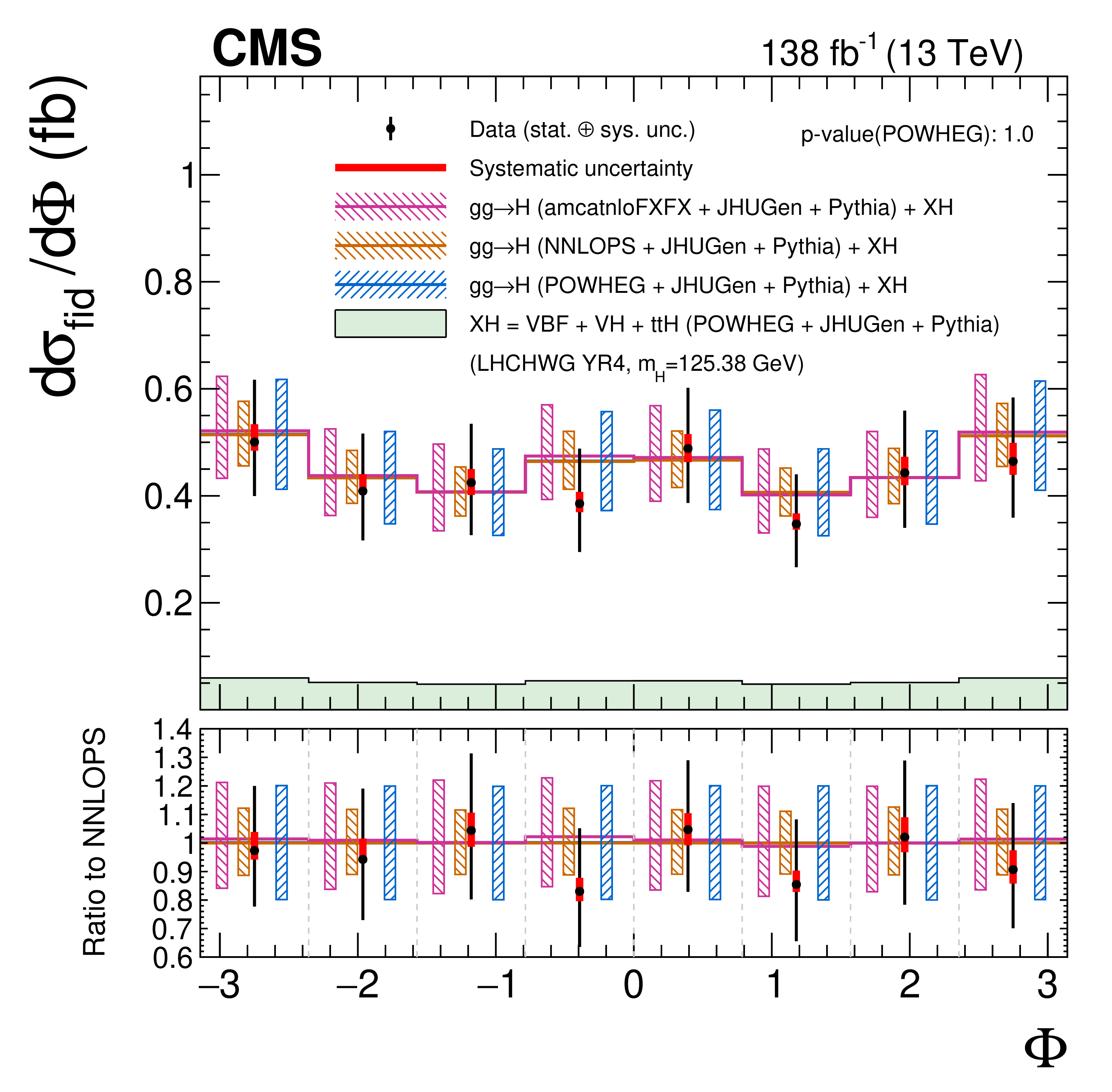
Figure 16-a:
Differential cross sections as functions of the $ \Phi $ angle in the 4$ \ell $ final states. The acceptance and theoretical uncertainties in the differential bins are calculated using the ggH predictions from the POWHEG generator (blue) normalized to $ \mathrm{N^3LO} $. The subdominant component of the signal (VBF+VH+ttH) is denoted as XH and is fixed to the SM prediction. The measured cross sections are also compared with the ggH predictions from NNLOPS (orange) and MadGraph-5_aMC@NLO (pink). The hatched areas correspond to the systematic uncertainties in the theoretical predictions. Black points represent the measured fiducial cross sections in each bin, black error bars the total uncertainty in each measurement, red boxes the systematic uncertainties. The lower panel displays the ratios of the measured cross sections and of the predictions from POWHEG and MadGraph-5_aMC@NLO to the NNLOPS theoretical predictions. |
png pdf |
Figure 16-b:
Differential cross sections as functions of the $ \Phi $ angle in the same-flavor final states. The acceptance and theoretical uncertainties in the differential bins are calculated using the ggH predictions from the POWHEG generator (blue) normalized to $ \mathrm{N^3LO} $. The subdominant component of the signal (VBF+VH+ttH) is denoted as XH and is fixed to the SM prediction. The measured cross sections are also compared with the ggH predictions from NNLOPS (orange) and MadGraph-5_aMC@NLO (pink). The hatched areas correspond to the systematic uncertainties in the theoretical predictions. Black points represent the measured fiducial cross sections in each bin, black error bars the total uncertainty in each measurement, red boxes the systematic uncertainties. The lower panel displays the ratios of the measured cross sections and of the predictions from POWHEG and MadGraph-5_aMC@NLO to the NNLOPS theoretical predictions. |
png pdf |
Figure 16-c:
Differential cross sections as functions of the $ \Phi $ angle in the different-flavor final states. The acceptance and theoretical uncertainties in the differential bins are calculated using the ggH predictions from the POWHEG generator (blue) normalized to $ \mathrm{N^3LO} $. The subdominant component of the signal (VBF+VH+ttH) is denoted as XH and is fixed to the SM prediction. The measured cross sections are also compared with the ggH predictions from NNLOPS (orange) and MadGraph-5_aMC@NLO (pink). The hatched areas correspond to the systematic uncertainties in the theoretical predictions. Black points represent the measured fiducial cross sections in each bin, black error bars the total uncertainty in each measurement, red boxes the systematic uncertainties. The lower panel displays the ratios of the measured cross sections and of the predictions from POWHEG and MadGraph-5_aMC@NLO to the NNLOPS theoretical predictions. |

png pdf |
Figure 17:
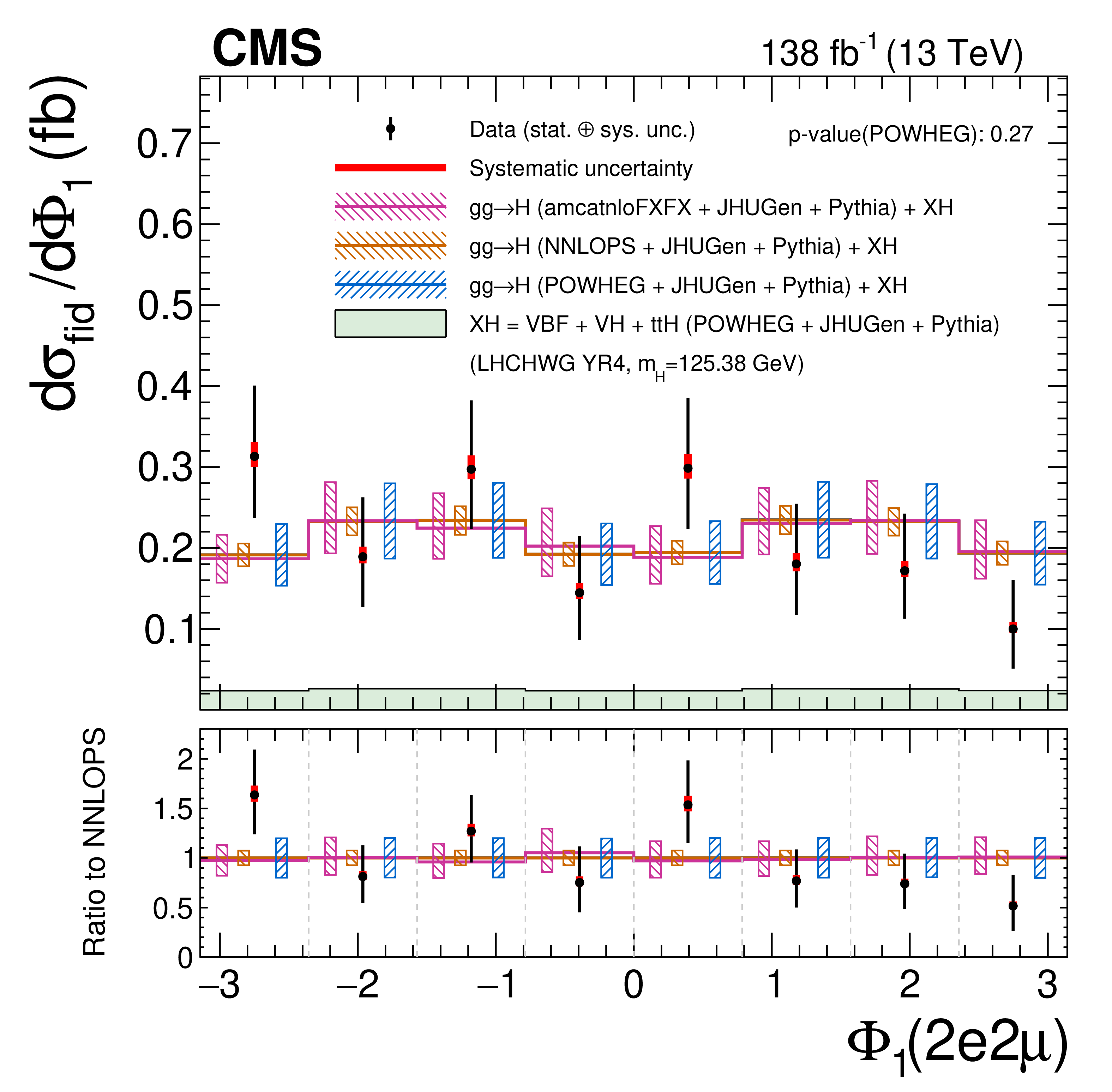
Differential cross sections as functions of the $ \Phi_\text{1} $ angle in the 4$ \ell $ (upper) and in the same-flavor (lower left) and different-flavor (lower right) final states. The acceptance and theoretical uncertainties in the differential bins are calculated using the ggH predictions from the POWHEG generator (blue) normalized to $ \mathrm{N^3LO} $. The subdominant component of the signal (VBF+VH+ttH) is denoted as XH and is fixed to the SM prediction. The measured cross sections are also compared with the ggH predictions from NNLOPS (orange) and MadGraph-5_aMC@NLO (pink). The hatched areas correspond to the systematic uncertainties in the theoretical predictions. Black points represent the measured fiducial cross sections in each bin, black error bars the total uncertainty in each measurement, red boxes the systematic uncertainties. The lower panels display the ratios of the measured cross sections and of the predictions from POWHEG and MadGraph-5_aMC@NLO to the NNLOPS theoretical predictions. |

png pdf |
Figure 17-a:
Differential cross sections as functions of the $ \Phi_\text{1} $ angle in the 4$ \ell $ final states. The acceptance and theoretical uncertainties in the differential bins are calculated using the ggH predictions from the POWHEG generator (blue) normalized to $ \mathrm{N^3LO} $. The subdominant component of the signal (VBF+VH+ttH) is denoted as XH and is fixed to the SM prediction. The measured cross sections are also compared with the ggH predictions from NNLOPS (orange) and MadGraph-5_aMC@NLO (pink). The hatched areas correspond to the systematic uncertainties in the theoretical predictions. Black points represent the measured fiducial cross sections in each bin, black error bars the total uncertainty in each measurement, red boxes the systematic uncertainties. The lower panel displays the ratios of the measured cross sections and of the predictions from POWHEG and MadGraph-5_aMC@NLO to the NNLOPS theoretical predictions. |

png pdf |
Figure 17-b:
Differential cross sections as functions of the $ \Phi_\text{1} $ angle in the same-flavor final states. The acceptance and theoretical uncertainties in the differential bins are calculated using the ggH predictions from the POWHEG generator (blue) normalized to $ \mathrm{N^3LO} $. The subdominant component of the signal (VBF+VH+ttH) is denoted as XH and is fixed to the SM prediction. The measured cross sections are also compared with the ggH predictions from NNLOPS (orange) and MadGraph-5_aMC@NLO (pink). The hatched areas correspond to the systematic uncertainties in the theoretical predictions. Black points represent the measured fiducial cross sections in each bin, black error bars the total uncertainty in each measurement, red boxes the systematic uncertainties. The lower panel displays the ratios of the measured cross sections and of the predictions from POWHEG and MadGraph-5_aMC@NLO to the NNLOPS theoretical predictions. |
png pdf |
Figure 17-c:
Differential cross sections as functions of the $ \Phi_\text{1} $ angle in the different-flavor final states. The acceptance and theoretical uncertainties in the differential bins are calculated using the ggH predictions from the POWHEG generator (blue) normalized to $ \mathrm{N^3LO} $. The subdominant component of the signal (VBF+VH+ttH) is denoted as XH and is fixed to the SM prediction. The measured cross sections are also compared with the ggH predictions from NNLOPS (orange) and MadGraph-5_aMC@NLO (pink). The hatched areas correspond to the systematic uncertainties in the theoretical predictions. Black points represent the measured fiducial cross sections in each bin, black error bars the total uncertainty in each measurement, red boxes the systematic uncertainties. The lower panel displays the ratios of the measured cross sections and of the predictions from POWHEG and MadGraph-5_aMC@NLO to the NNLOPS theoretical predictions. |
png pdf |
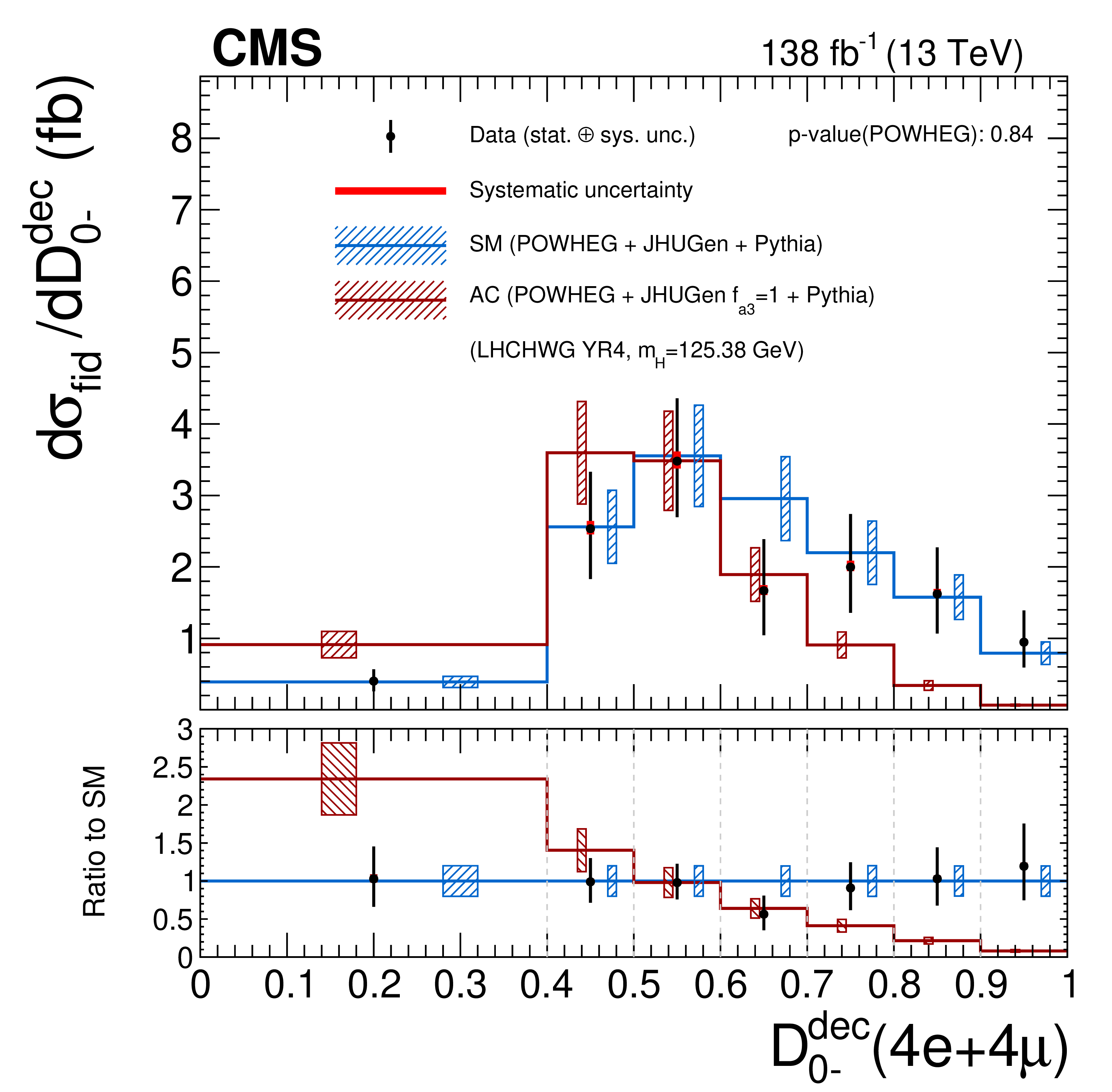
Figure 18:
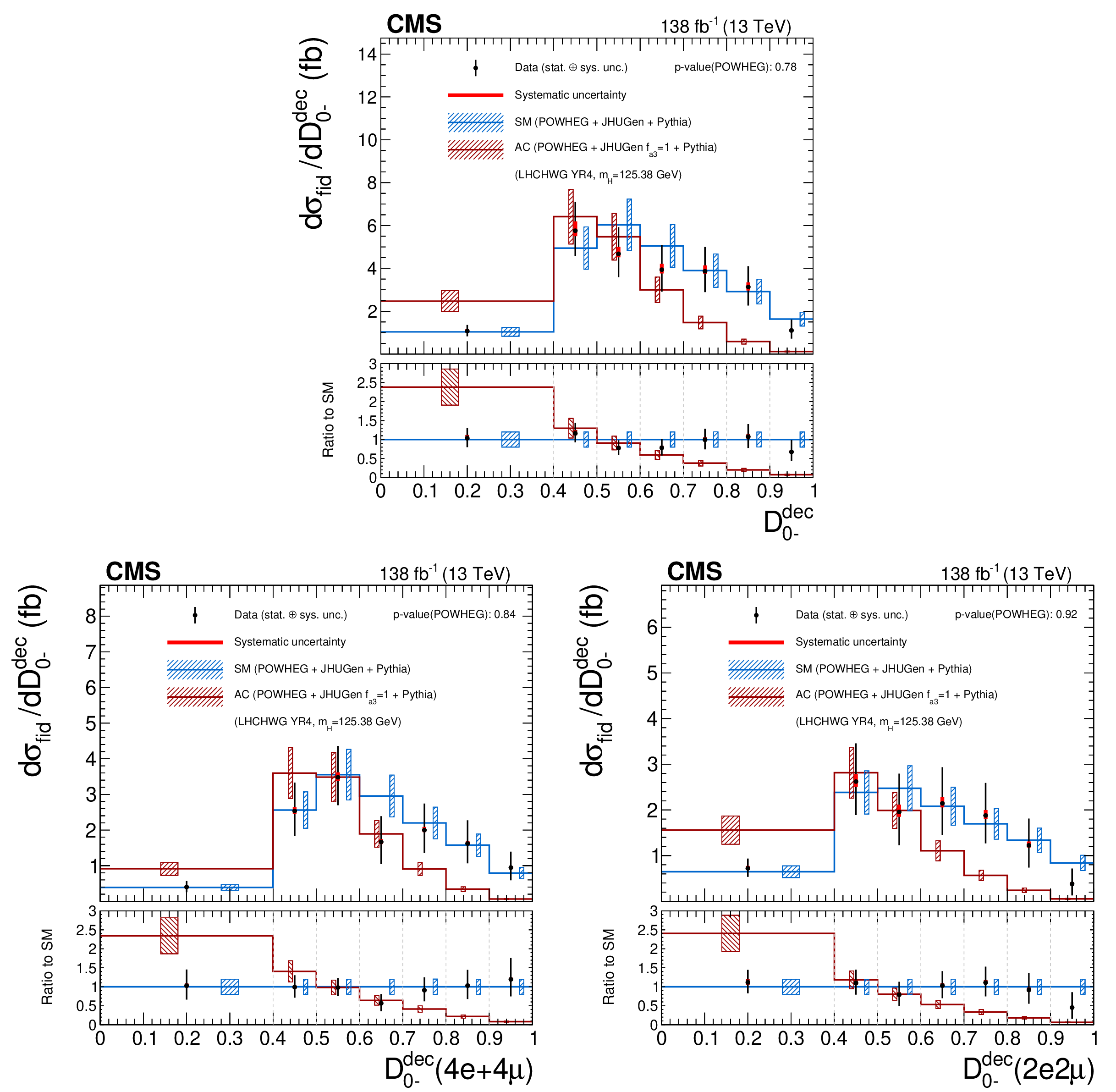
Differential cross sections as functions of the matrix element kinematic discriminant $ {\mathcal D}^{\text{dec}}_{\text{0-}} $ in the 4$ \ell $ (upper) and in the same-flavor (lower left) and different-flavor (lower right) final states. The brown histograms show the distribution of the matrix element discriminant for the HVV anomalous coupling scenario corresponding to $ f_{a3} = $ 1. The subdominant component of the signal (VBF+VH+ttH) is fixed to the SM prediction. The hatched areas correspond to the systematic uncertainties in the theoretical predictions. Black points represent the measured fiducial cross sections in each bin, black error bars the total uncertainty in each measurement, red boxes the systematic uncertainties. The lower panels display the ratios of the measured cross sections and of the predictions from POWHEG and MadGraph-5_aMC@NLO to the NNLOPS theoretical predictions. |

png pdf |
Figure 18-a:
Differential cross sections as functions of the matrix element kinematic discriminant $ {\mathcal D}^{\text{dec}}_{\text{0-}} $ in the 4$ \ell $ final states. The brown histograms show the distribution of the matrix element discriminant for the HVV anomalous coupling scenario corresponding to $ f_{a3} = $ 1. The subdominant component of the signal (VBF+VH+ttH) is fixed to the SM prediction. The hatched areas correspond to the systematic uncertainties in the theoretical predictions. Black points represent the measured fiducial cross sections in each bin, black error bars the total uncertainty in each measurement, red boxes the systematic uncertainties. The lower panel displays the ratios of the measured cross sections and of the predictions from POWHEG and MadGraph-5_aMC@NLO to the NNLOPS theoretical predictions. |
png pdf |
Figure 18-b:
Differential cross sections as functions of the matrix element kinematic discriminant $ {\mathcal D}^{\text{dec}}_{\text{0-}} $ in the same-flavor final states. The brown histograms show the distribution of the matrix element discriminant for the HVV anomalous coupling scenario corresponding to $ f_{a3} = $ 1. The subdominant component of the signal (VBF+VH+ttH) is fixed to the SM prediction. The hatched areas correspond to the systematic uncertainties in the theoretical predictions. Black points represent the measured fiducial cross sections in each bin, black error bars the total uncertainty in each measurement, red boxes the systematic uncertainties. The lower panel displays the ratios of the measured cross sections and of the predictions from POWHEG and MadGraph-5_aMC@NLO to the NNLOPS theoretical predictions. |
png pdf |
Figure 18-c:
Differential cross sections as functions of the matrix element kinematic discriminant $ {\mathcal D}^{\text{dec}}_{\text{0-}} $ in the different-flavor final states. The brown histograms show the distribution of the matrix element discriminant for the HVV anomalous coupling scenario corresponding to $ f_{a3} = $ 1. The subdominant component of the signal (VBF+VH+ttH) is fixed to the SM prediction. The hatched areas correspond to the systematic uncertainties in the theoretical predictions. Black points represent the measured fiducial cross sections in each bin, black error bars the total uncertainty in each measurement, red boxes the systematic uncertainties. The lower panel displays the ratios of the measured cross sections and of the predictions from POWHEG and MadGraph-5_aMC@NLO to the NNLOPS theoretical predictions. |
png pdf |
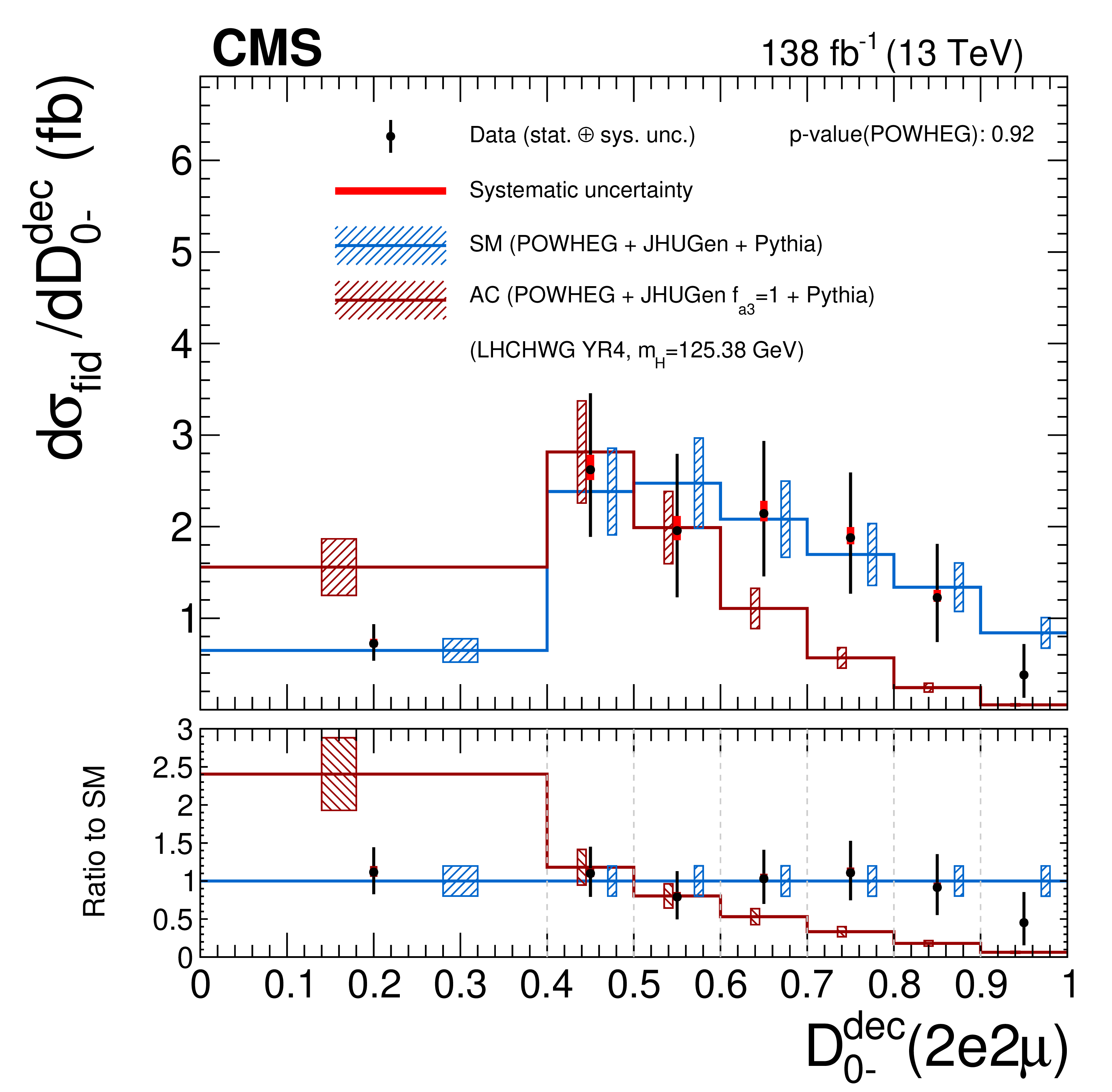
Figure 19:
Differential cross sections as functions of the matrix element kinematic discriminant $ {\mathcal D}^{\text{dec}}_{\text{0h+}} $ in the 4$ \ell $ (upper) and in the same-flavor (lower left) and different-flavor (lower right) final states. The brown histograms show the distribution of the matrix element discriminant for the HVV anomalous coupling scenario corresponding to $ f_{a2} = $ 1. The subdominant component of the signal (VBF+VH+ttH) is fixed to the SM prediction. The hatched areas correspond to the systematic uncertainties in the theoretical predictions. Black points represent the measured fiducial cross sections in each bin, black error bars the total uncertainty in each measurement, red boxes the systematic uncertainties. The lower panels display the ratios of the measured cross sections and of the predictions from POWHEG and MadGraph-5_aMC@NLO to the NNLOPS theoretical predictions. |

png pdf |
Figure 19-a:
Differential cross sections as functions of the matrix element kinematic discriminant $ {\mathcal D}^{\text{dec}}_{\text{0h+}} $ in the 4$ \ell $ final states. The brown histograms show the distribution of the matrix element discriminant for the HVV anomalous coupling scenario corresponding to $ f_{a2} = $ 1. The subdominant component of the signal (VBF+VH+ttH) is fixed to the SM prediction. The hatched areas correspond to the systematic uncertainties in the theoretical predictions. Black points represent the measured fiducial cross sections in each bin, black error bars the total uncertainty in each measurement, red boxes the systematic uncertainties. The lower panel displays the ratios of the measured cross sections and of the predictions from POWHEG and MadGraph-5_aMC@NLO to the NNLOPS theoretical predictions. |

png pdf |
Figure 19-b:
Differential cross sections as functions of the matrix element kinematic discriminant $ {\mathcal D}^{\text{dec}}_{\text{0h+}} $ in the same-flavor final states. The brown histograms show the distribution of the matrix element discriminant for the HVV anomalous coupling scenario corresponding to $ f_{a2} = $ 1. The subdominant component of the signal (VBF+VH+ttH) is fixed to the SM prediction. The hatched areas correspond to the systematic uncertainties in the theoretical predictions. Black points represent the measured fiducial cross sections in each bin, black error bars the total uncertainty in each measurement, red boxes the systematic uncertainties. The lower panel displays the ratios of the measured cross sections and of the predictions from POWHEG and MadGraph-5_aMC@NLO to the NNLOPS theoretical predictions. |

png pdf |
Figure 19-c:
Differential cross sections as functions of the matrix element kinematic discriminant $ {\mathcal D}^{\text{dec}}_{\text{0h+}} $ in the different-flavor final states. The brown histograms show the distribution of the matrix element discriminant for the HVV anomalous coupling scenario corresponding to $ f_{a2} = $ 1. The subdominant component of the signal (VBF+VH+ttH) is fixed to the SM prediction. The hatched areas correspond to the systematic uncertainties in the theoretical predictions. Black points represent the measured fiducial cross sections in each bin, black error bars the total uncertainty in each measurement, red boxes the systematic uncertainties. The lower panel displays the ratios of the measured cross sections and of the predictions from POWHEG and MadGraph-5_aMC@NLO to the NNLOPS theoretical predictions. |
png pdf |
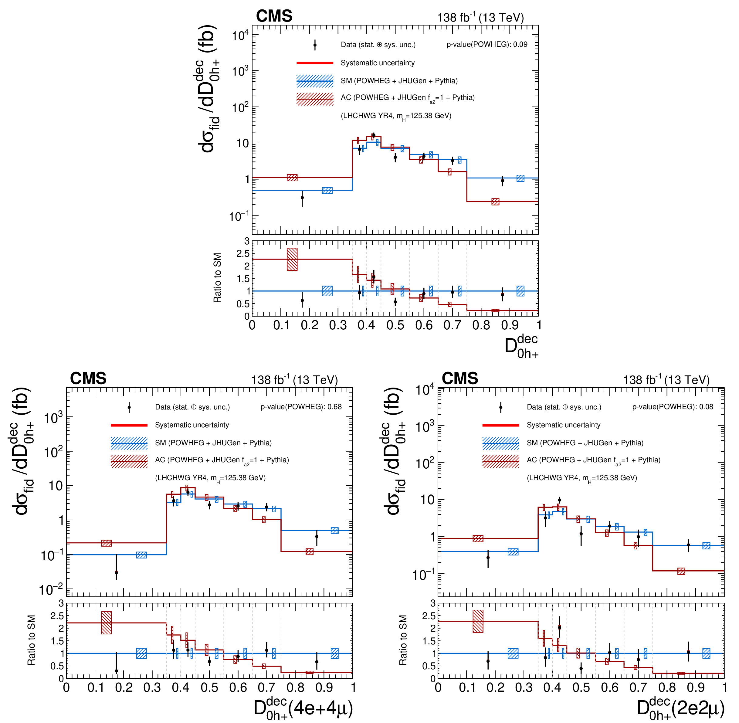
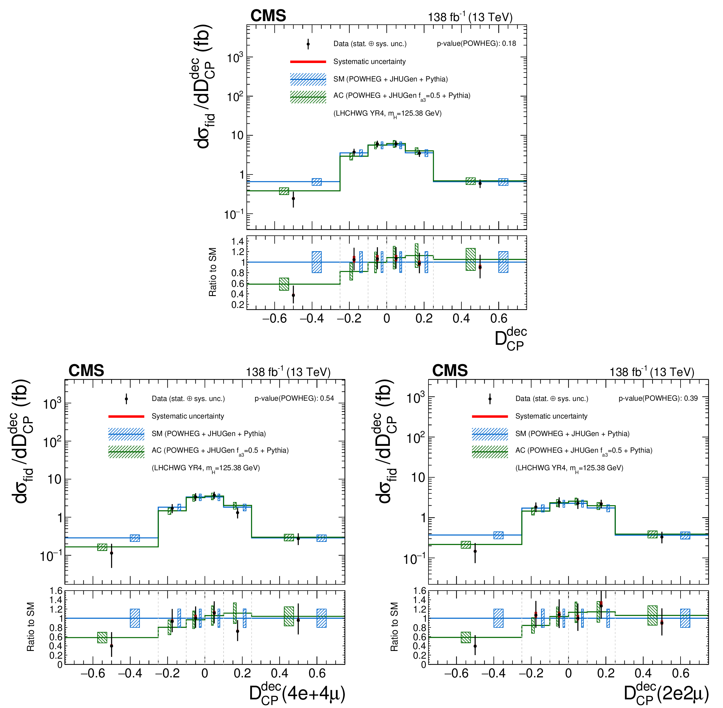
Figure 20:
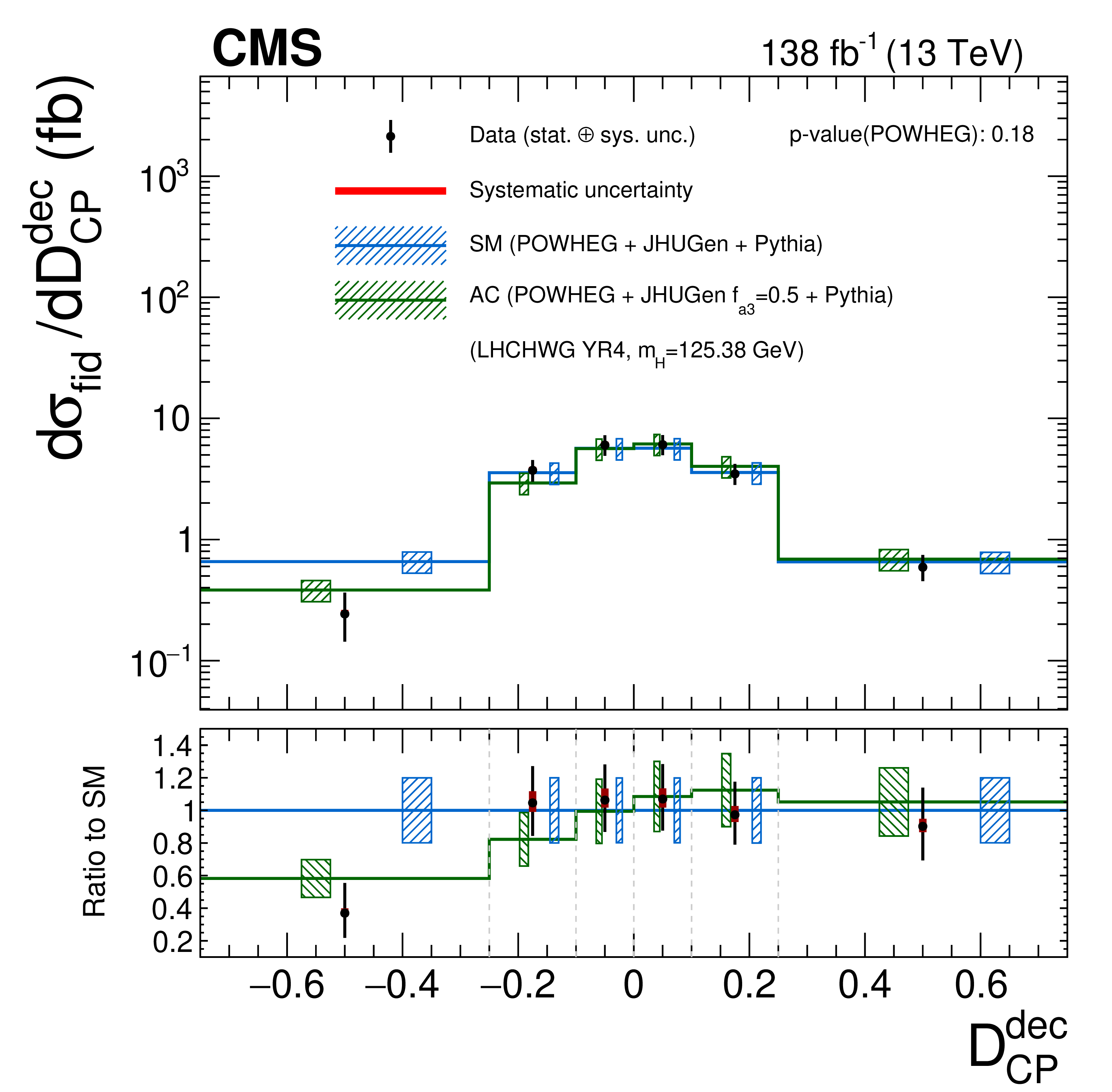
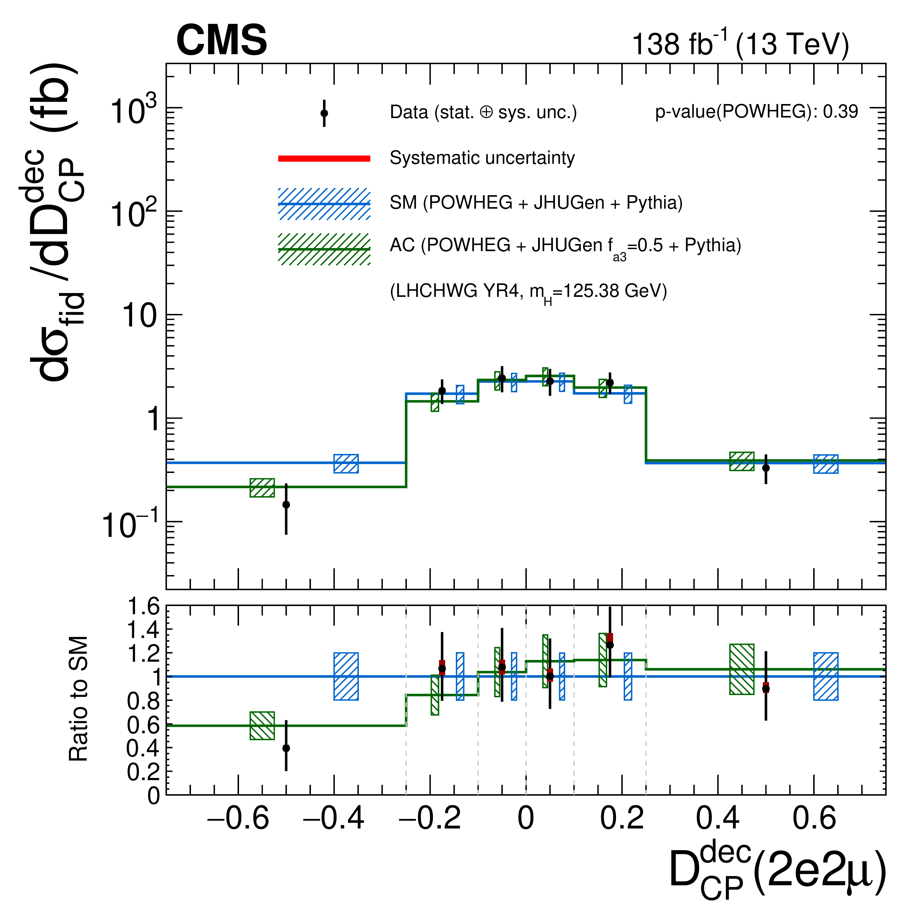
Differential cross sections as functions of the matrix element kinematic discriminant $ {\mathcal D}^{\text{dec}}_{\text{CP}} $ in the 4$ \ell $ (upper) and in the same-flavor (lower left) and different-flavor (lower right) final states. The green histogram shows the distribution of the discriminant for the HVV anomalous coupling scenario corresponding to $ f_{a3} = $ 0.5. The subdominant component of the signal (VBF+VH+ttH) is fixed to the SM prediction. The hatched areas correspond to the systematic uncertainties in the theoretical predictions. Black points represent the measured fiducial cross sections in each bin, black error bars the total uncertainty in each measurement, red boxes the systematic uncertainties. The lower panels display the ratios of the measured cross sections and of the predictions from POWHEG and MadGraph-5_aMC@NLO to the NNLOPS theoretical predictions. |
png pdf |
Figure 20-a:
Differential cross sections as functions of the matrix element kinematic discriminant $ {\mathcal D}^{\text{dec}}_{\text{CP}} $ in the 4$ \ell $ final states. The green histogram shows the distribution of the discriminant for the HVV anomalous coupling scenario corresponding to $ f_{a3} = $ 0.5. The subdominant component of the signal (VBF+VH+ttH) is fixed to the SM prediction. The hatched areas correspond to the systematic uncertainties in the theoretical predictions. Black points represent the measured fiducial cross sections in each bin, black error bars the total uncertainty in each measurement, red boxes the systematic uncertainties. The lower panel displays the ratios of the measured cross sections and of the predictions from POWHEG and MadGraph-5_aMC@NLO to the NNLOPS theoretical predictions. |
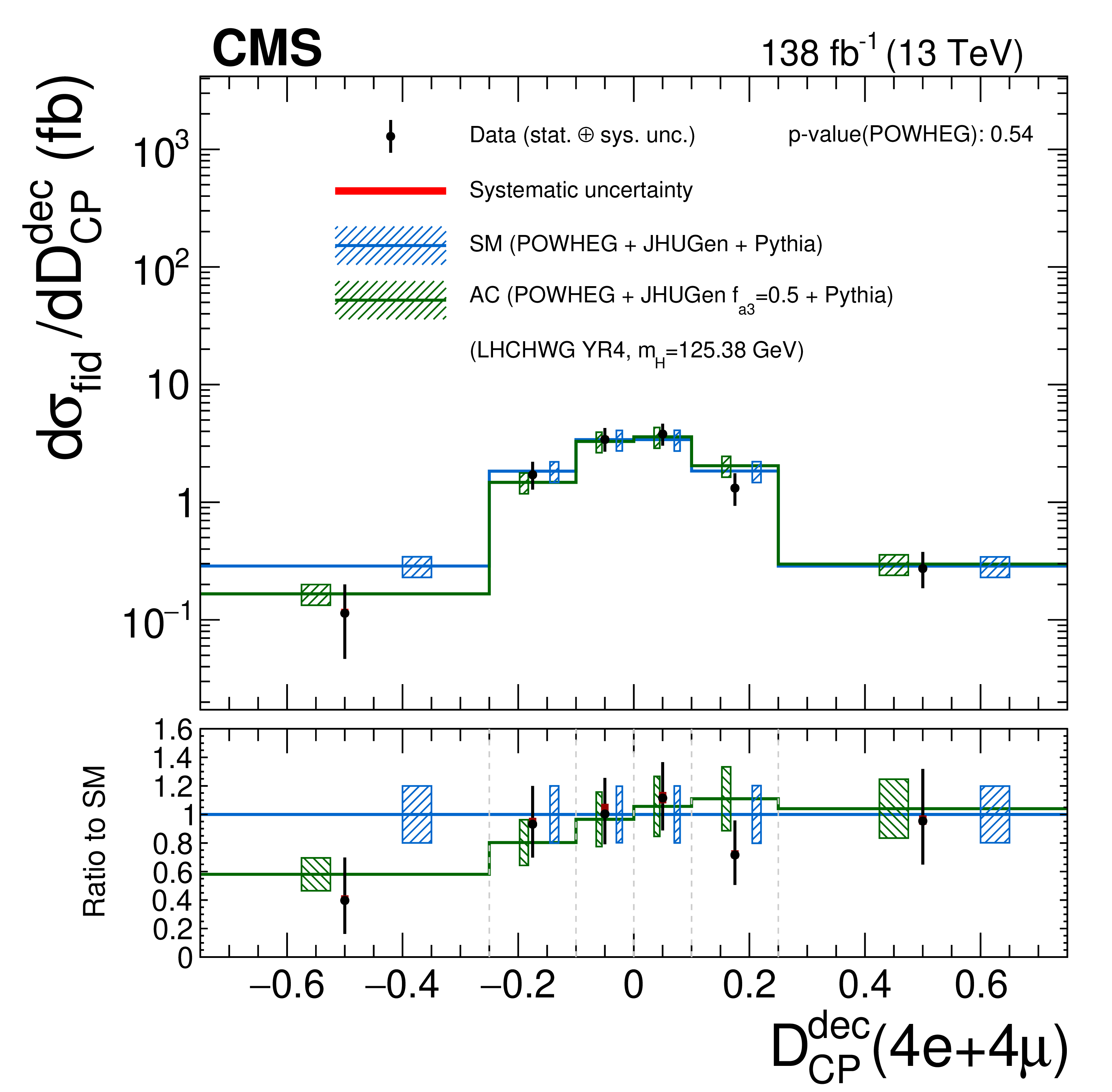
png pdf |
Figure 20-b:
Differential cross sections as functions of the matrix element kinematic discriminant $ {\mathcal D}^{\text{dec}}_{\text{CP}} $ in the same-flavor final states. The green histogram shows the distribution of the discriminant for the HVV anomalous coupling scenario corresponding to $ f_{a3} = $ 0.5. The subdominant component of the signal (VBF+VH+ttH) is fixed to the SM prediction. The hatched areas correspond to the systematic uncertainties in the theoretical predictions. Black points represent the measured fiducial cross sections in each bin, black error bars the total uncertainty in each measurement, red boxes the systematic uncertainties. The lower panel displays the ratios of the measured cross sections and of the predictions from POWHEG and MadGraph-5_aMC@NLO to the NNLOPS theoretical predictions. |
png pdf |
Figure 20-c:
Differential cross sections as functions of the matrix element kinematic discriminant $ {\mathcal D}^{\text{dec}}_{\text{CP}} $ in the different-flavor final states. The green histogram shows the distribution of the discriminant for the HVV anomalous coupling scenario corresponding to $ f_{a3} = $ 0.5. The subdominant component of the signal (VBF+VH+ttH) is fixed to the SM prediction. The hatched areas correspond to the systematic uncertainties in the theoretical predictions. Black points represent the measured fiducial cross sections in each bin, black error bars the total uncertainty in each measurement, red boxes the systematic uncertainties. The lower panel displays the ratios of the measured cross sections and of the predictions from POWHEG and MadGraph-5_aMC@NLO to the NNLOPS theoretical predictions. |
png pdf |
Figure 21:
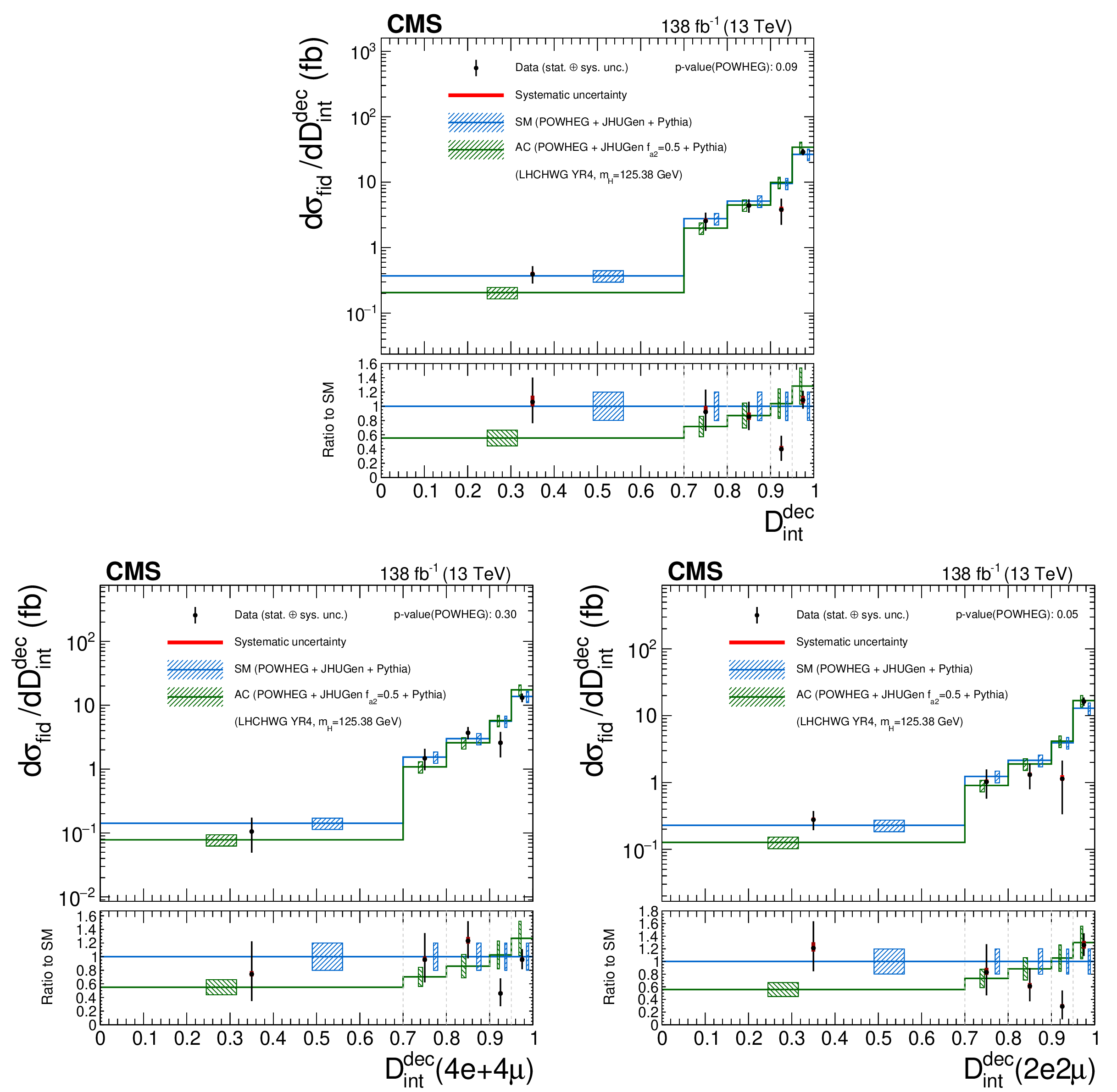
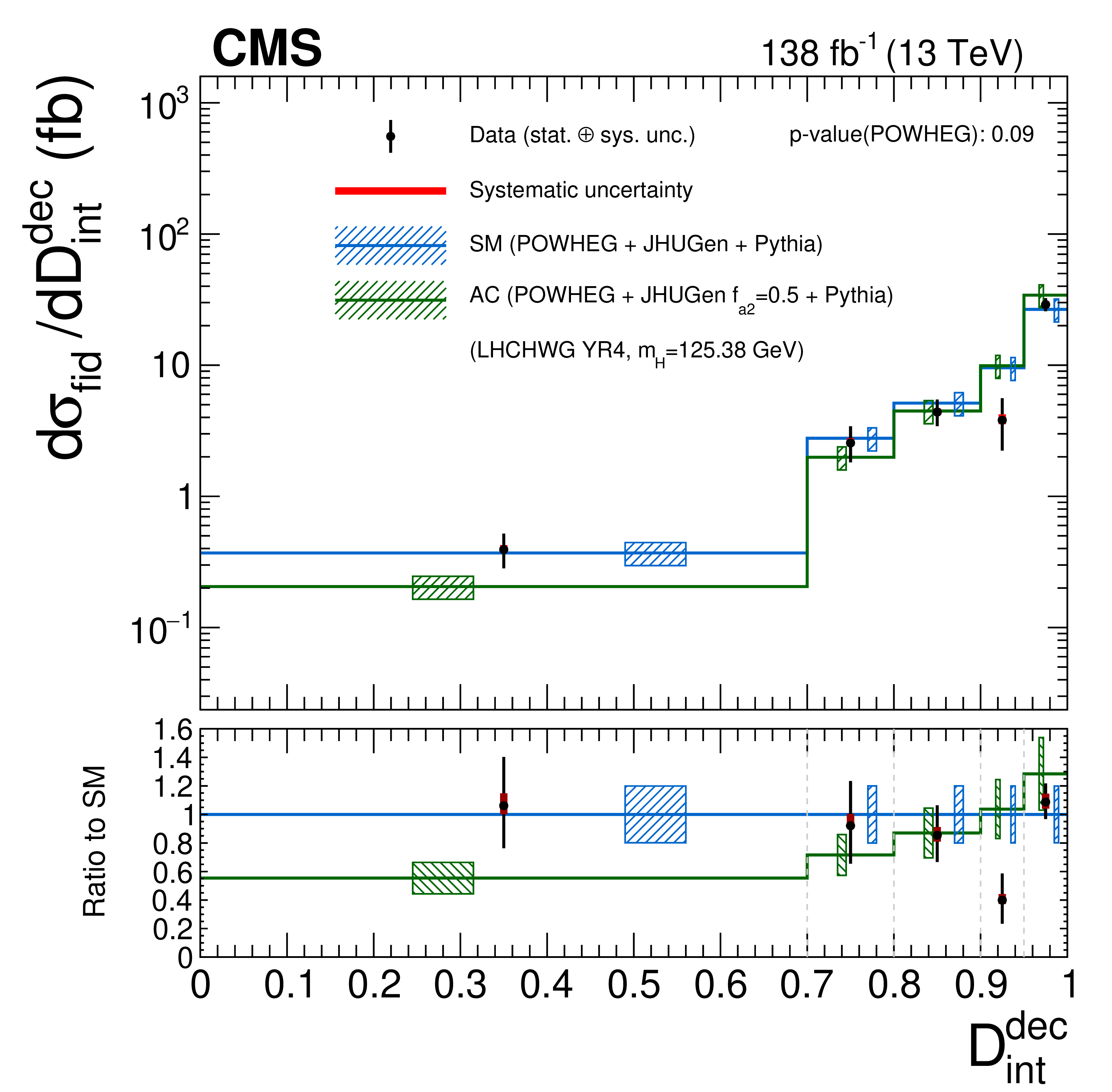
Differential cross sections as functions of the matrix element kinematic discriminant $ {\mathcal D}^{\text{dec}}_{\text{int}} $ in the 4$ \ell $ (upper) and in the same-flavor (lower left) and different-flavor (lower right) final states. The green histogram shows the distribution of the discriminant for the HVV anomalous coupling scenario corresponding to $ f_{a2} = $ 0.5. The subdominant component of the signal (VBF+VH+ttH) is fixed to the SM prediction. The hatched areas correspond to the systematic uncertainties in the theoretical predictions. Black points represent the measured fiducial cross sections in each bin, black error bars the total uncertainty in each measurement, red boxes the systematic uncertainties. The lower panels display the ratios of the measured cross sections and of the predictions from POWHEG and MadGraph-5_aMC@NLO to the NNLOPS theoretical predictions. |
png pdf |
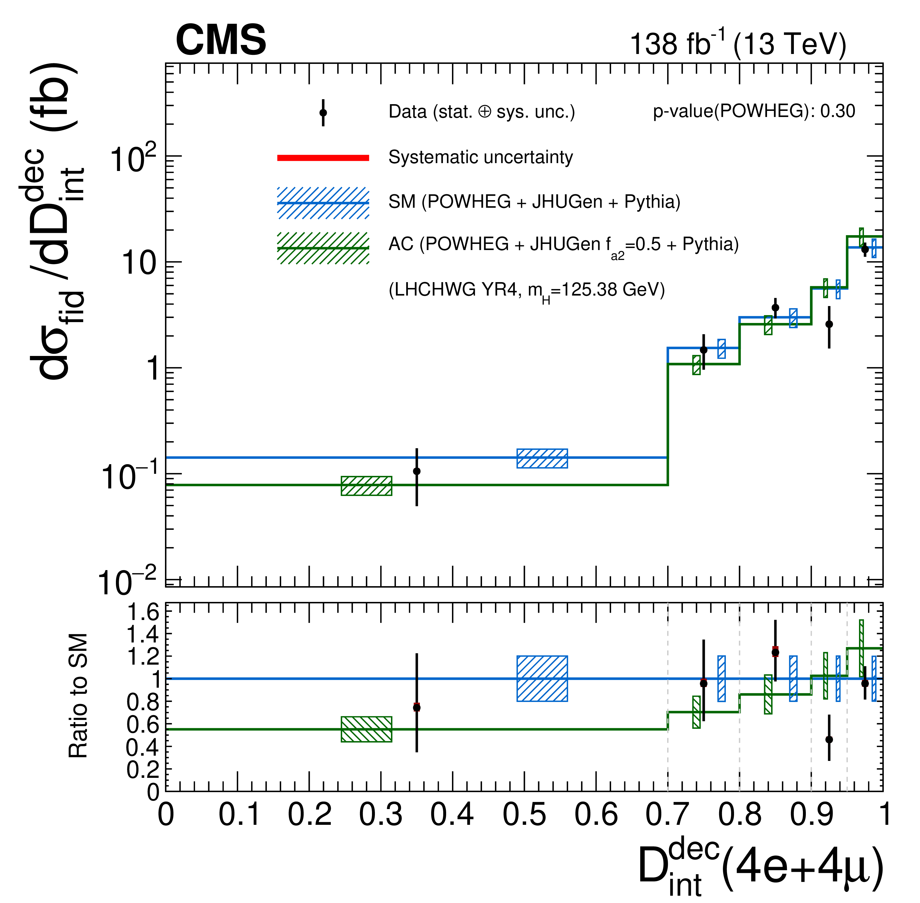
Figure 21-a:
Differential cross sections as functions of the matrix element kinematic discriminant $ {\mathcal D}^{\text{dec}}_{\text{int}} $ in the 4$ \ell $ final states. The green histogram shows the distribution of the discriminant for the HVV anomalous coupling scenario corresponding to $ f_{a2} = $ 0.5. The subdominant component of the signal (VBF+VH+ttH) is fixed to the SM prediction. The hatched areas correspond to the systematic uncertainties in the theoretical predictions. Black points represent the measured fiducial cross sections in each bin, black error bars the total uncertainty in each measurement, red boxes the systematic uncertainties. The lower panel displays the ratios of the measured cross sections and of the predictions from POWHEG and MadGraph-5_aMC@NLO to the NNLOPS theoretical predictions. |
png pdf |
Figure 21-b:
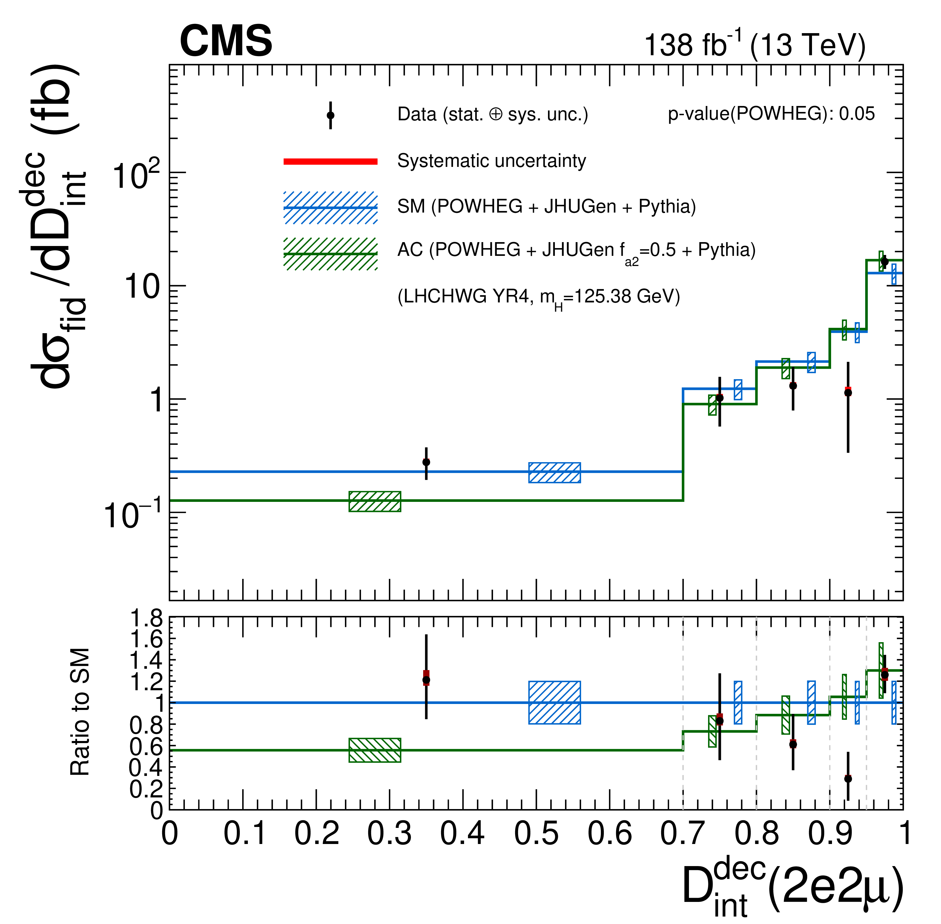
Differential cross sections as functions of the matrix element kinematic discriminant $ {\mathcal D}^{\text{dec}}_{\text{int}} $ in the same-flavor final states. The green histogram shows the distribution of the discriminant for the HVV anomalous coupling scenario corresponding to $ f_{a2} = $ 0.5. The subdominant component of the signal (VBF+VH+ttH) is fixed to the SM prediction. The hatched areas correspond to the systematic uncertainties in the theoretical predictions. Black points represent the measured fiducial cross sections in each bin, black error bars the total uncertainty in each measurement, red boxes the systematic uncertainties. The lower panel displays the ratios of the measured cross sections and of the predictions from POWHEG and MadGraph-5_aMC@NLO to the NNLOPS theoretical predictions. |
png pdf |
Figure 21-c:
Differential cross sections as functions of the matrix element kinematic discriminant $ {\mathcal D}^{\text{dec}}_{\text{int}} $ in the different-flavor final states. The green histogram shows the distribution of the discriminant for the HVV anomalous coupling scenario corresponding to $ f_{a2} = $ 0.5. The subdominant component of the signal (VBF+VH+ttH) is fixed to the SM prediction. The hatched areas correspond to the systematic uncertainties in the theoretical predictions. Black points represent the measured fiducial cross sections in each bin, black error bars the total uncertainty in each measurement, red boxes the systematic uncertainties. The lower panel displays the ratios of the measured cross sections and of the predictions from POWHEG and MadGraph-5_aMC@NLO to the NNLOPS theoretical predictions. |
png pdf |
Figure 22:
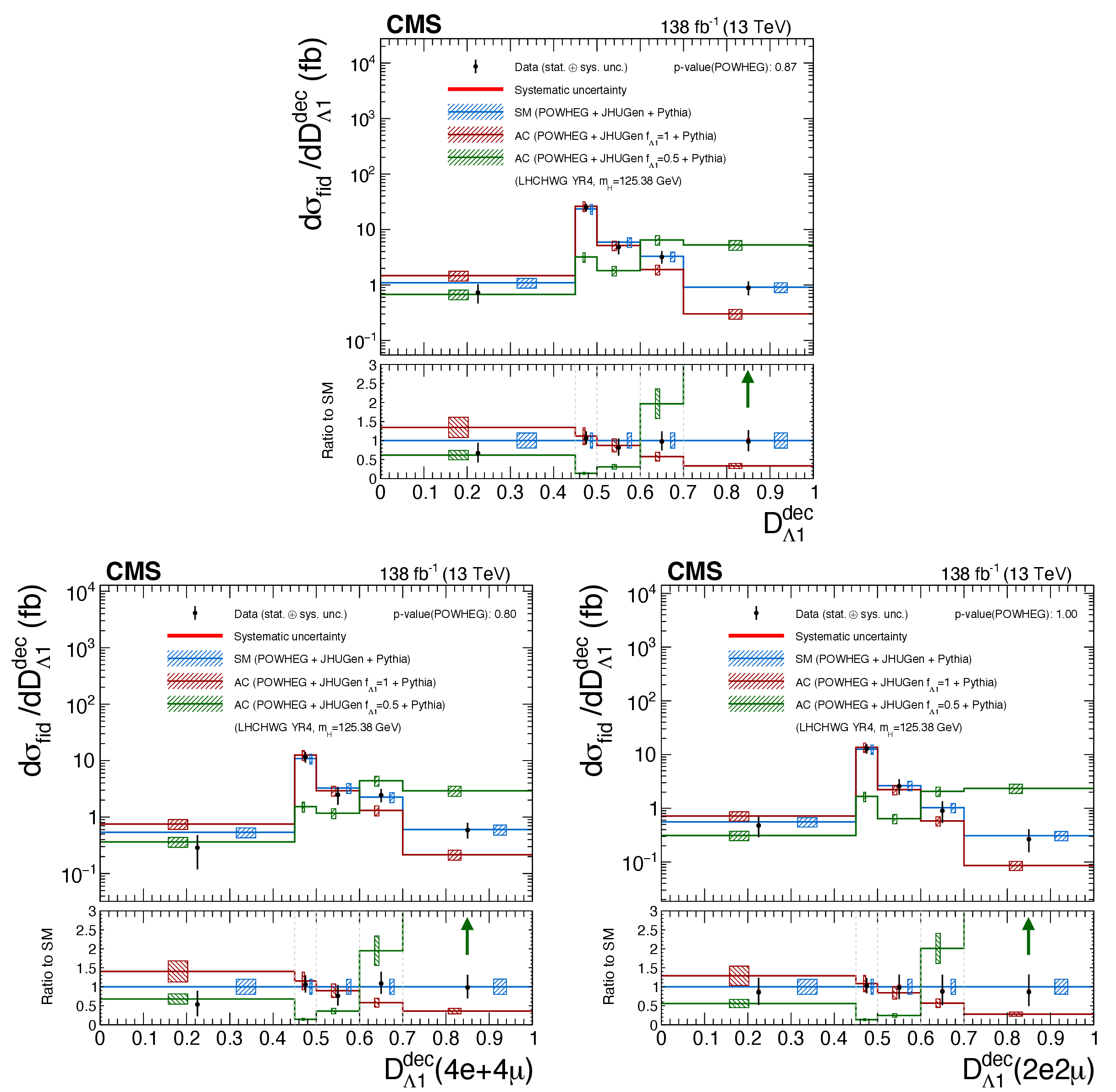
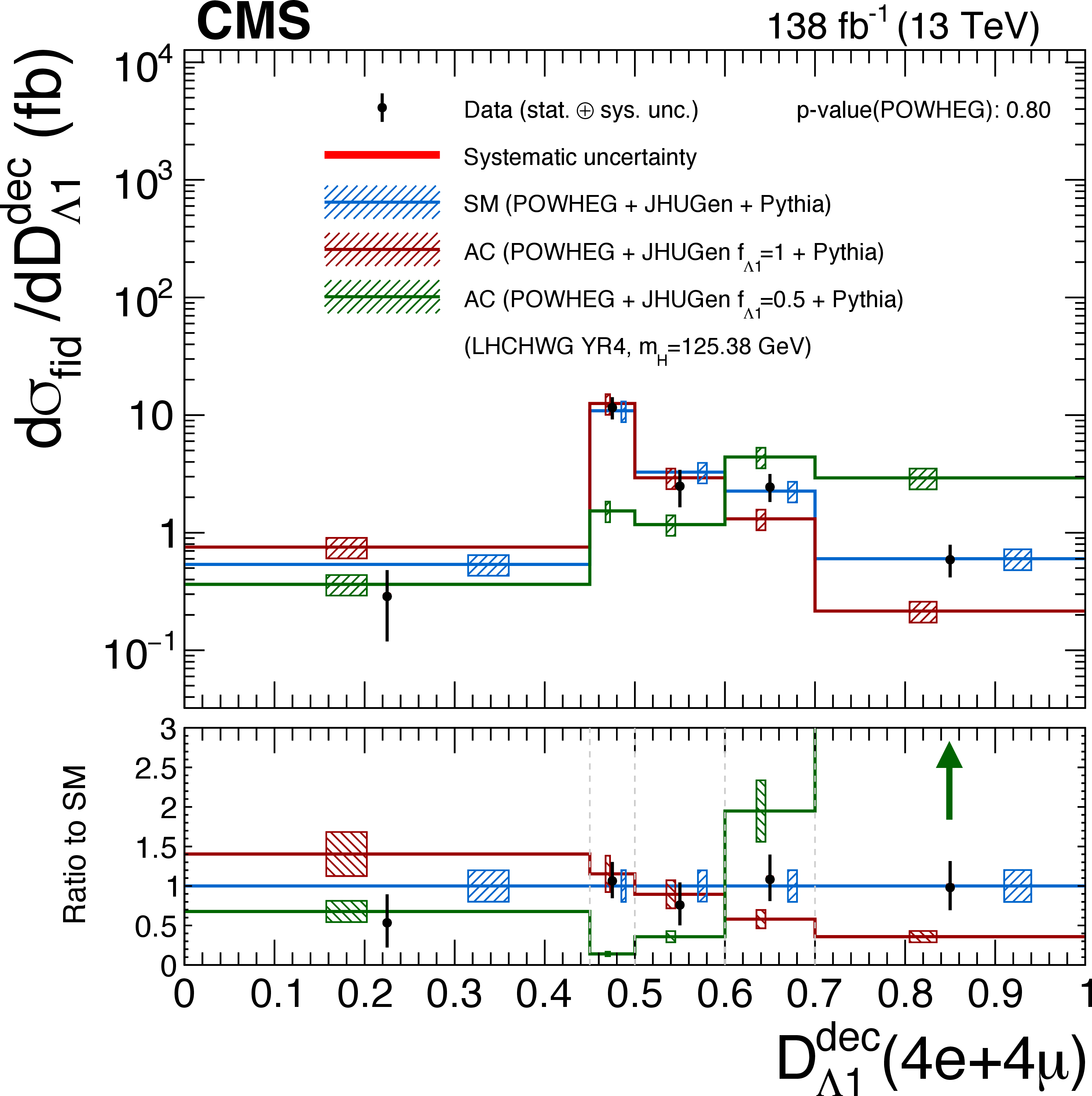
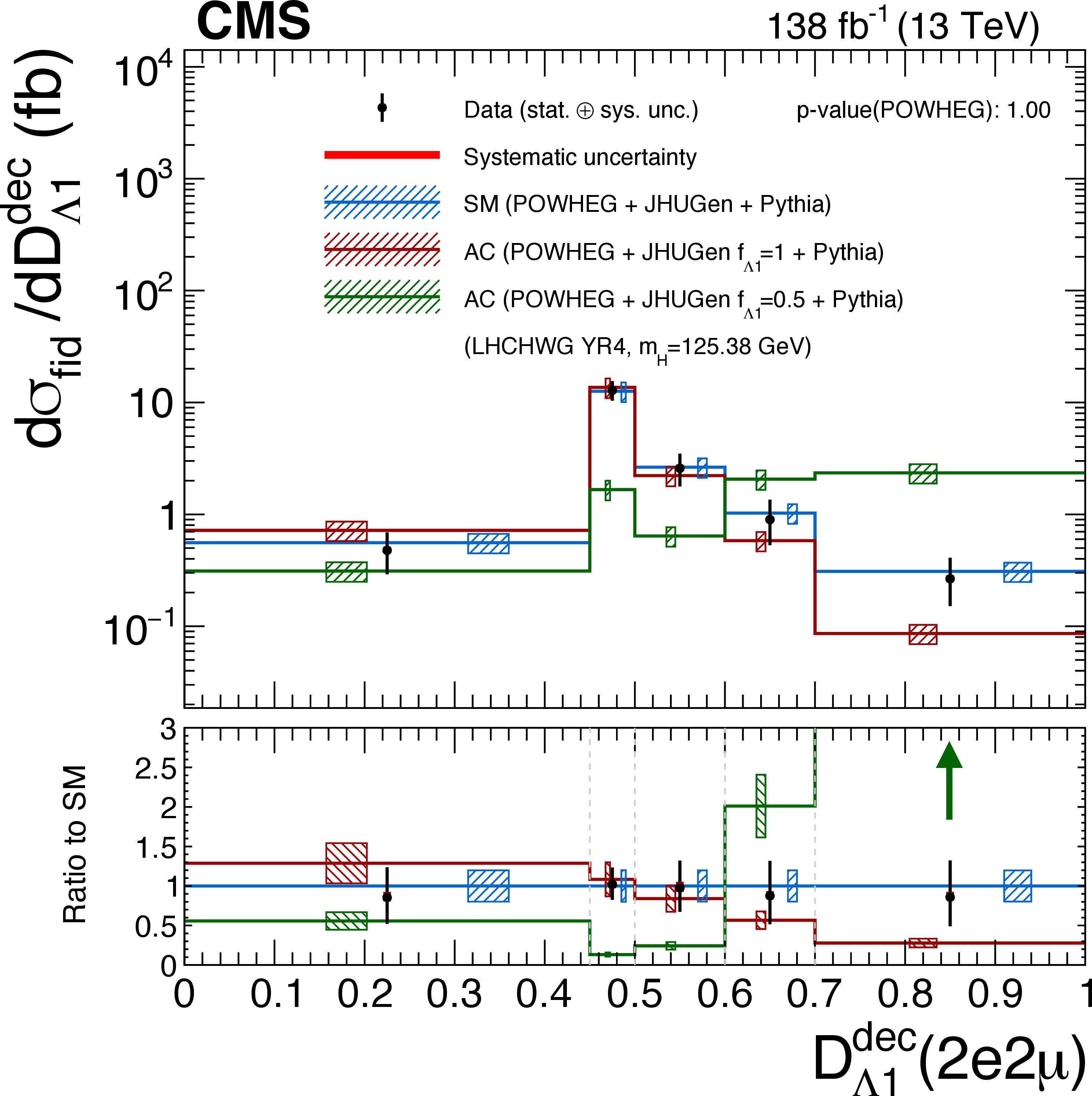
Differential cross sections as functions of the matrix element kinematic discriminant $ {\mathcal D}^{\text{dec}}_{\Lambda\text{1}} $ in the 4$ \ell $ (upper) and in the same-flavor (lower left) and different-flavor (lower right) final states. The brown and green histograms show the distributions of the discriminant for the HVV anomalous coupling scenarios corresponding to $ f_{\Lambda 1} = $ 1 and $ f_{\Lambda 1} = $ 0.5. The subdominant component of the signal (VBF+VH+ttH) is fixed to the SM prediction. The hatched areas correspond to the systematic uncertainties in the theoretical predictions. Black points represent the measured fiducial cross sections in each bin, black error bars the total uncertainty in each measurement, red boxes the systematic uncertainties. The lower panels display the ratio of the measured cross section and of the predictions from POWHEG and MadGraph-5_aMC@NLO to the NNLOPS theoretical expectation. |

png pdf |
Figure 22-a:
Differential cross sections as functions of the matrix element kinematic discriminant $ {\mathcal D}^{\text{dec}}_{\Lambda\text{1}} $ in the 4$ \ell $ final states. The brown and green histograms show the distributions of the discriminant for the HVV anomalous coupling scenarios corresponding to $ f_{\Lambda 1} = $ 1 and $ f_{\Lambda 1} = $ 0.5. The subdominant component of the signal (VBF+VH+ttH) is fixed to the SM prediction. The hatched areas correspond to the systematic uncertainties in the theoretical predictions. Black points represent the measured fiducial cross sections in each bin, black error bars the total uncertainty in each measurement, red boxes the systematic uncertainties. The lower panel displays the ratio of the measured cross section and of the predictions from POWHEG and MadGraph-5_aMC@NLO to the NNLOPS theoretical expectation. |
png pdf |
Figure 22-b:
Differential cross sections as functions of the matrix element kinematic discriminant $ {\mathcal D}^{\text{dec}}_{\Lambda\text{1}} $ in the same-flavor final states. The brown and green histograms show the distributions of the discriminant for the HVV anomalous coupling scenarios corresponding to $ f_{\Lambda 1} = $ 1 and $ f_{\Lambda 1} = $ 0.5. The subdominant component of the signal (VBF+VH+ttH) is fixed to the SM prediction. The hatched areas correspond to the systematic uncertainties in the theoretical predictions. Black points represent the measured fiducial cross sections in each bin, black error bars the total uncertainty in each measurement, red boxes the systematic uncertainties. The lower panel displays the ratio of the measured cross section and of the predictions from POWHEG and MadGraph-5_aMC@NLO to the NNLOPS theoretical expectation. |
png pdf |
Figure 22-c:
Differential cross sections as functions of the matrix element kinematic discriminant $ {\mathcal D}^{\text{dec}}_{\Lambda\text{1}} $ in the different-flavor final states. The brown and green histograms show the distributions of the discriminant for the HVV anomalous coupling scenarios corresponding to $ f_{\Lambda 1} = $ 1 and $ f_{\Lambda 1} = $ 0.5. The subdominant component of the signal (VBF+VH+ttH) is fixed to the SM prediction. The hatched areas correspond to the systematic uncertainties in the theoretical predictions. Black points represent the measured fiducial cross sections in each bin, black error bars the total uncertainty in each measurement, red boxes the systematic uncertainties. The lower panel displays the ratio of the measured cross section and of the predictions from POWHEG and MadGraph-5_aMC@NLO to the NNLOPS theoretical expectation. |

png pdf |
Figure 23:
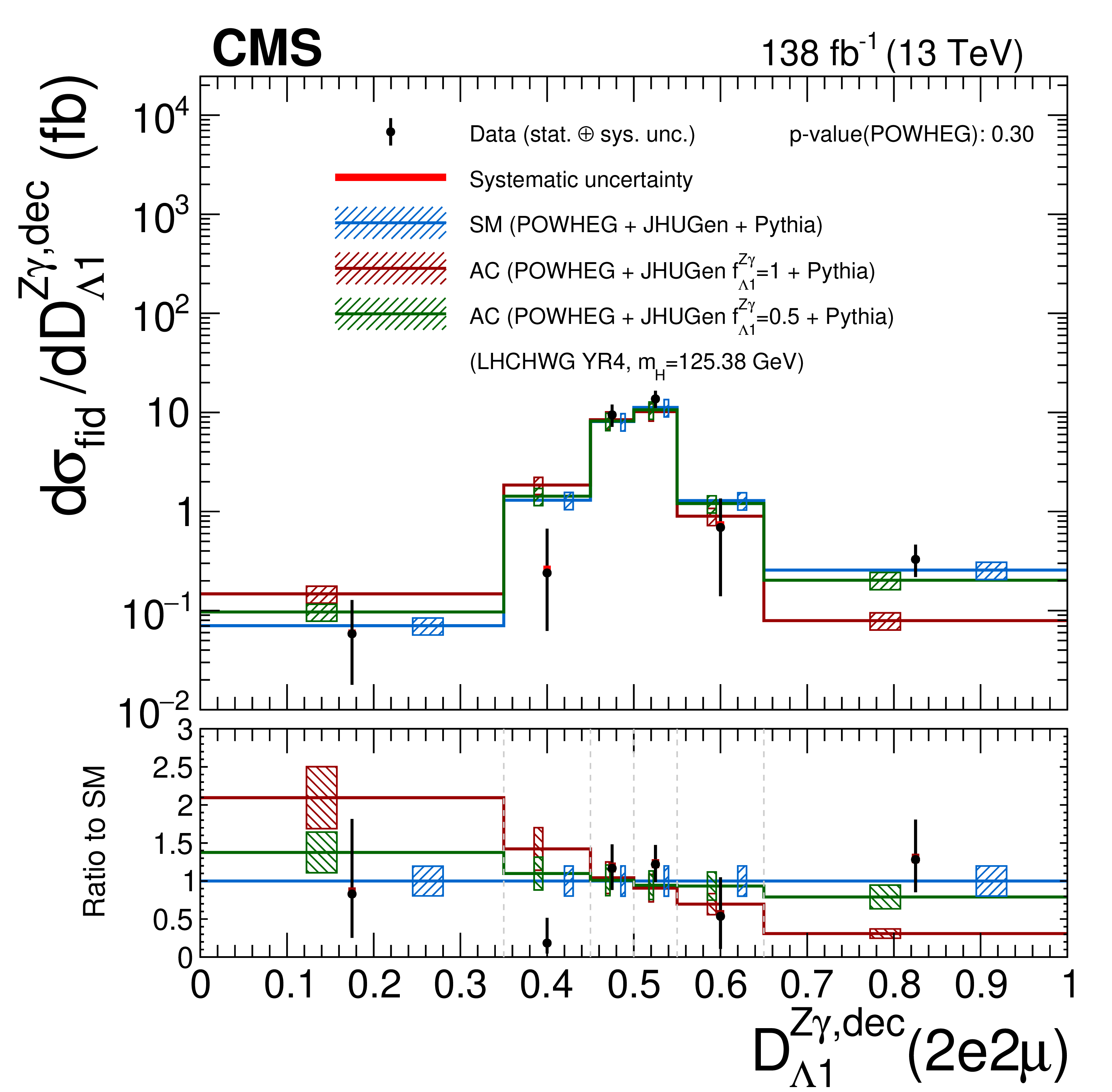
Differential cross sections as functions of the matrix element kinematic discriminant $ {\mathcal D}_{\Lambda\text{1}}^{\mathrm{Z}\gamma, \text{dec}} $ in the 4$ \ell $ (upper) and in the same-flavor (lower left) and different-flavor (lower right) final states. The brown and green histograms show the distributions of the discriminant for the HVV anomalous coupling scenarios corresponding to $ f_{\Lambda 1}^{\mathrm{Z}\gamma} = $ 1 and $ f_{\Lambda 1}^{\mathrm{Z}\gamma} = $ 0.5. The subdominant component of the signal (VBF+VH+ttH) is fixed to the SM prediction. The hatched areas correspond to the systematic uncertainties in the theoretical predictions. Black points represent the measured fiducial cross sections in each bin, black error bars the total uncertainty in each measurement, red boxes the systematic uncertainties. The lower panels display the ratios of the measured cross sections and of the predictions from POWHEG and MadGraph-5_aMC@NLO to the NNLOPS theoretical predictions. |

png pdf |
Figure 23-a:
Differential cross sections as functions of the matrix element kinematic discriminant $ {\mathcal D}_{\Lambda\text{1}}^{\mathrm{Z}\gamma, \text{dec}} $ in the 4$ \ell $ final states. The brown and green histograms show the distributions of the discriminant for the HVV anomalous coupling scenarios corresponding to $ f_{\Lambda 1}^{\mathrm{Z}\gamma} = $ 1 and $ f_{\Lambda 1}^{\mathrm{Z}\gamma} = $ 0.5. The subdominant component of the signal (VBF+VH+ttH) is fixed to the SM prediction. The hatched areas correspond to the systematic uncertainties in the theoretical predictions. Black points represent the measured fiducial cross sections in each bin, black error bars the total uncertainty in each measurement, red boxes the systematic uncertainties. The lower panel displays the ratios of the measured cross sections and of the predictions from POWHEG and MadGraph-5_aMC@NLO to the NNLOPS theoretical predictions. |

png pdf |
Figure 23-b:
Differential cross sections as functions of the matrix element kinematic discriminant $ {\mathcal D}_{\Lambda\text{1}}^{\mathrm{Z}\gamma, \text{dec}} $ in the same-flavor final states. The brown and green histograms show the distributions of the discriminant for the HVV anomalous coupling scenarios corresponding to $ f_{\Lambda 1}^{\mathrm{Z}\gamma} = $ 1 and $ f_{\Lambda 1}^{\mathrm{Z}\gamma} = $ 0.5. The subdominant component of the signal (VBF+VH+ttH) is fixed to the SM prediction. The hatched areas correspond to the systematic uncertainties in the theoretical predictions. Black points represent the measured fiducial cross sections in each bin, black error bars the total uncertainty in each measurement, red boxes the systematic uncertainties. The lower panel displays the ratios of the measured cross sections and of the predictions from POWHEG and MadGraph-5_aMC@NLO to the NNLOPS theoretical predictions. |
png pdf |
Figure 23-c:
Differential cross sections as functions of the matrix element kinematic discriminant $ {\mathcal D}_{\Lambda\text{1}}^{\mathrm{Z}\gamma, \text{dec}} $ in the different-flavor final states. The brown and green histograms show the distributions of the discriminant for the HVV anomalous coupling scenarios corresponding to $ f_{\Lambda 1}^{\mathrm{Z}\gamma} = $ 1 and $ f_{\Lambda 1}^{\mathrm{Z}\gamma} = $ 0.5. The subdominant component of the signal (VBF+VH+ttH) is fixed to the SM prediction. The hatched areas correspond to the systematic uncertainties in the theoretical predictions. Black points represent the measured fiducial cross sections in each bin, black error bars the total uncertainty in each measurement, red boxes the systematic uncertainties. The lower panel displays the ratios of the measured cross sections and of the predictions from POWHEG and MadGraph-5_aMC@NLO to the NNLOPS theoretical predictions. |

png pdf |
Figure 24:
Double differential cross sections in bins of $ |y_{\mathrm{H}}| $ vs. $ p_{\mathrm{T}}^{\mathrm{H}} $ (upper left), number of associated jets vs. $ p_{\mathrm{T}}^{\mathrm{H}} $ (upper right), and $ \mathcal{T}_{\text{C}}^{\text{max}} $ vs. $ p_{\mathrm{T}}^{\mathrm{H}} $ (lower). The binnings of the various measurements are reported in Table 6. The content of each plot is described in the caption of Fig. 6. |
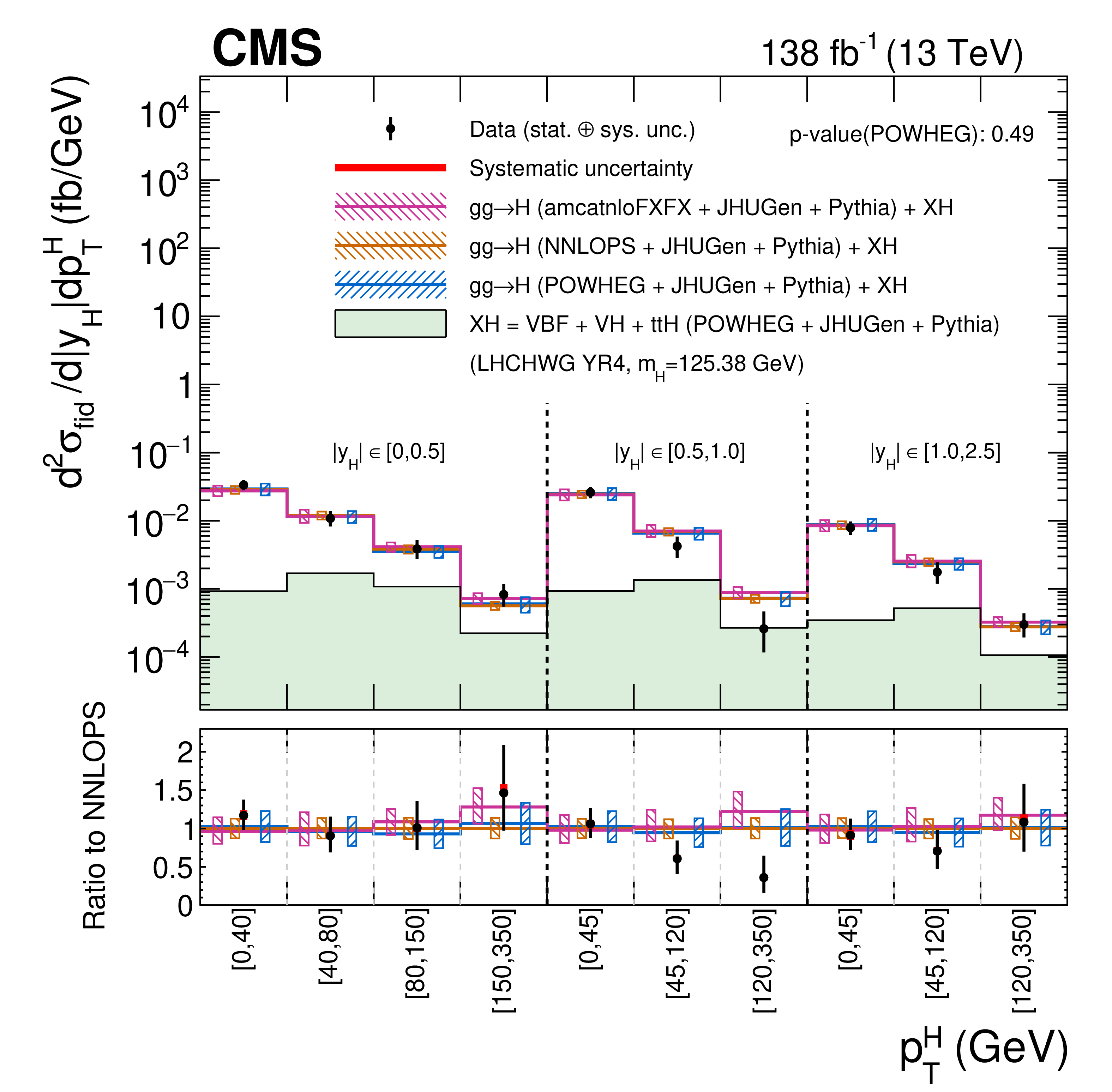
png pdf |
Figure 24-a:
Double differential cross sections in bins of $ |y_{\mathrm{H}}| $ vs. $ p_{\mathrm{T}}^{\mathrm{H}} $. The binnings of the measurements are reported in Table 6. The content of the plot is described in the caption of Fig. 6. |

png pdf |
Figure 24-b:
Double differential cross sections in bins of number of associated jets vs. $ p_{\mathrm{T}}^{\mathrm{H}} $. The binnings of the measurements are reported in Table 6. The content of the plot is described in the caption of Fig. 6. |
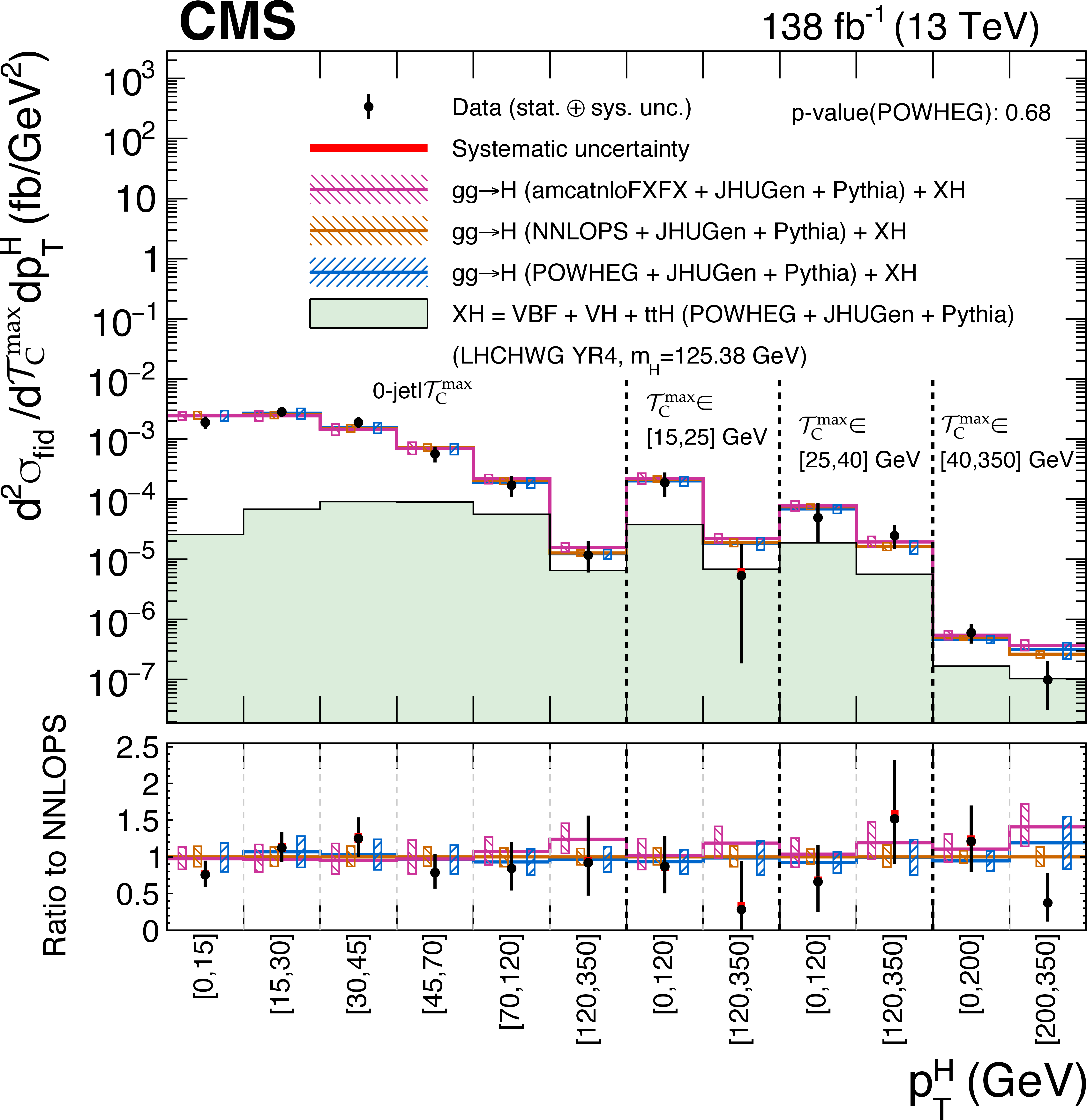
png pdf |
Figure 24-c:
Double differential cross sections in bins of $ \mathcal{T}_{\text{C}}^{\text{max}} $ vs. $ p_{\mathrm{T}}^{\mathrm{H}} $. The binnings of the measurements are reported in Table 6. The content of the plot is described in the caption of Fig. 6. |

png pdf |
Figure 25:
Double differential cross sections in bins of $ p_{\mathrm{T}}^{\mathrm{H} \text{j}} $ vs. $ p_{\mathrm{T}}^{\mathrm{H}} $ (upper left), $ m_{\mathrm{Z}_{1}} $ vs. $ m_{\mathrm{Z}_{2}} $ (upper right), and $ p_{\mathrm{T}} $ of the leading vs. subleading jet (lower). The binnings of the various measurements are reported in Table 6. The content of each plot is described in the caption of Fig. 6. |
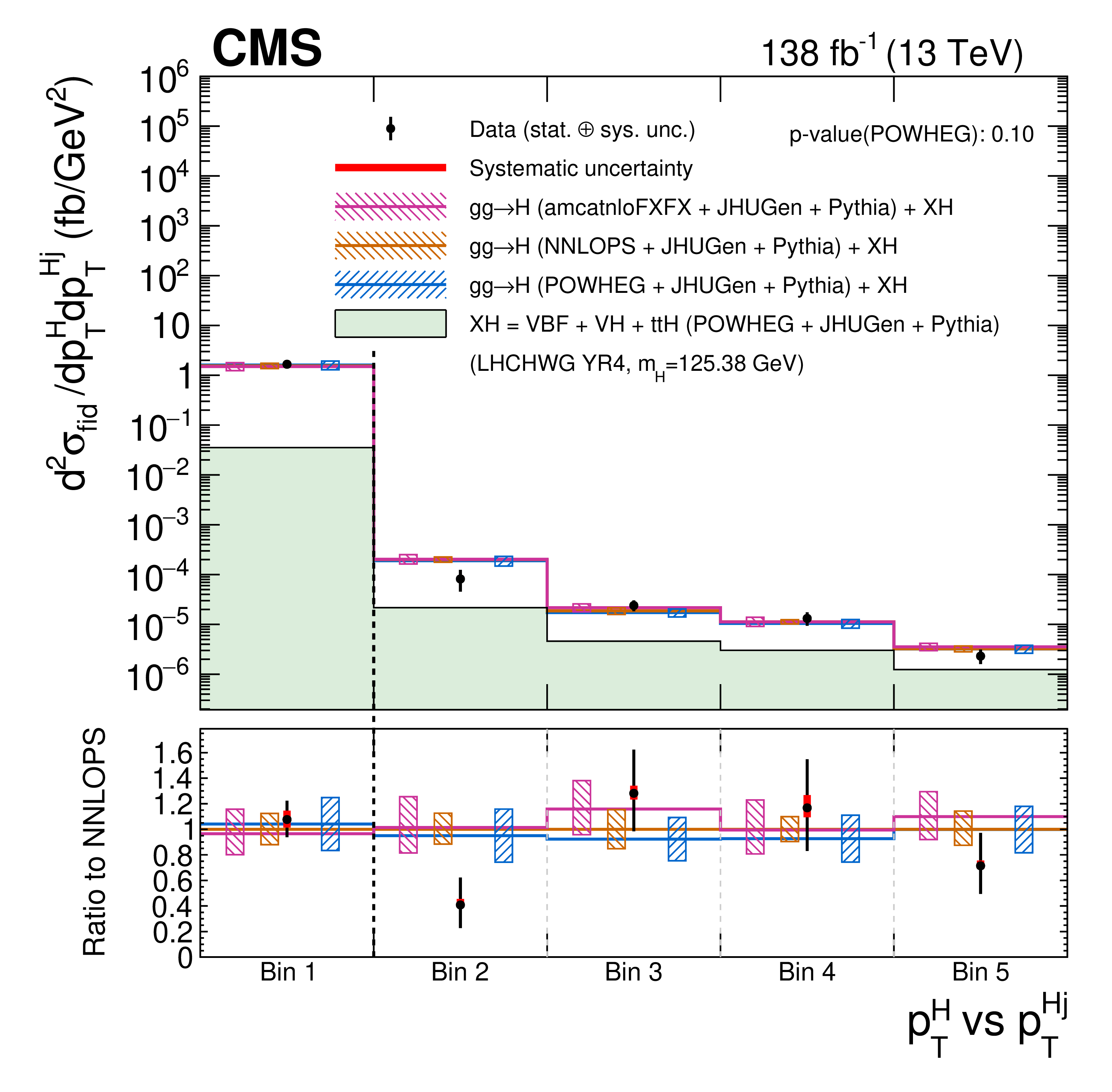
png pdf |
Figure 25-a:
Double differential cross sections in bins of $ p_{\mathrm{T}}^{\mathrm{H} \text{j}} $ vs. $ p_{\mathrm{T}}^{\mathrm{H}} $. The binnings of the measurements are reported in Table 6. The content of the plot is described in the caption of Fig. 6. |

png pdf |
Figure 25-b:
Double differential cross sections in bins of $ m_{\mathrm{Z}_{1}} $ vs. $ m_{\mathrm{Z}_{2}} $. The binnings of the measurements are reported in Table 6. The content of the plot is described in the caption of Fig. 6. |

png pdf |
Figure 25-c:
Double differential cross sections in bins of $ p_{\mathrm{T}} $ of the leading vs. subleading jet. The binnings of the measurements are reported in Table 6. The content of the plot is described in the caption of Fig. 6. |

png pdf |
Figure 26:
Likelihood scan as a function of $ \kappa_\lambda $. The scan is shown with (solid line) and without (dashed line) systematic uncertainties profiled in the fit. |
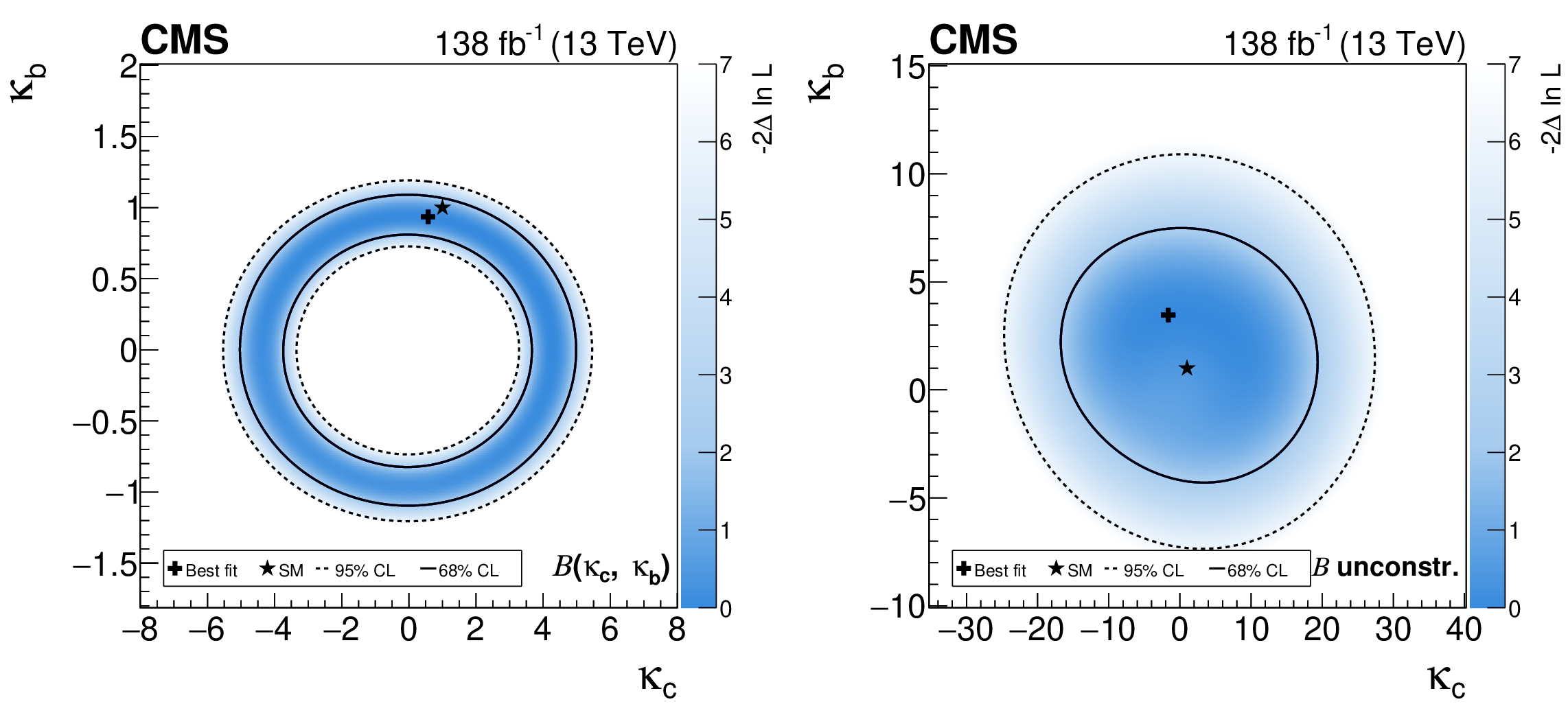
png pdf |
Figure 27:
Simultaneous fit of $ \kappa_\mathrm{b} $ and $ \kappa_\mathrm{c} $, assuming a coupling dependence of the branching fraction (left) and treating it as an unconstrained parameter in the fit (right). |

png pdf |
Figure 27-a:
Simultaneous fit of $ \kappa_\mathrm{b} $ and $ \kappa_\mathrm{c} $, assuming a coupling dependence of the branching fraction. |

png pdf |
Figure 27-b:
Simultaneous fit of $ \kappa_\mathrm{b} $ and $ \kappa_\mathrm{c} $, treating the branching fraction as an unconstrained parameter in the fit. |
| Tables | |

png pdf |
Table 1:
Thresholds applied on the $ p_{\mathrm{T}} $ of the leading/subleading leptons in each data-taking period for the main dielectron (e/e), dimuon ($ \mu $/$ \mu $), and electron-muon (e/$ \mu $, $ \mu $/e) HLT algorithms. |
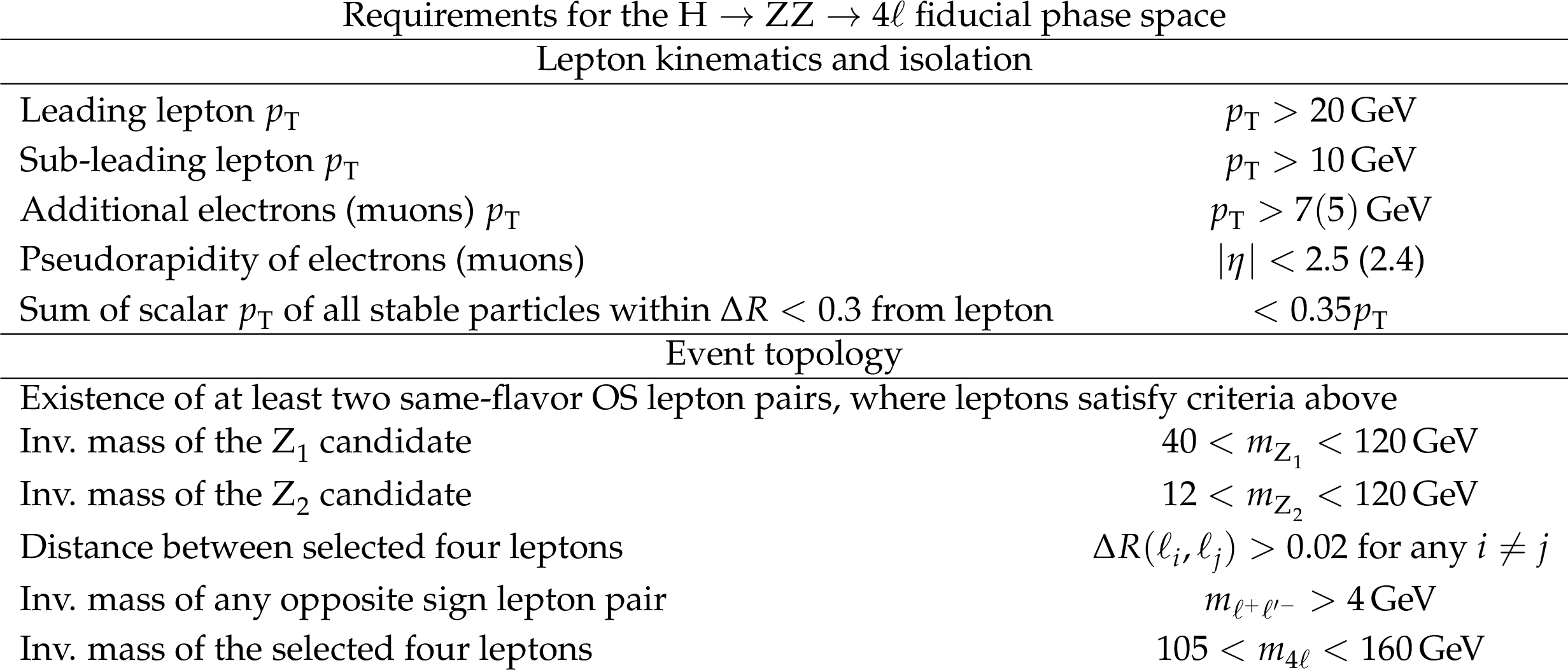
png pdf |
Table 2:
Summary of the requirements used in the definition of the fiducial phase space for the $ \mathrm{H}\to\mathrm{Z}\mathrm{Z}\to4\ell $ cross section measurements. |
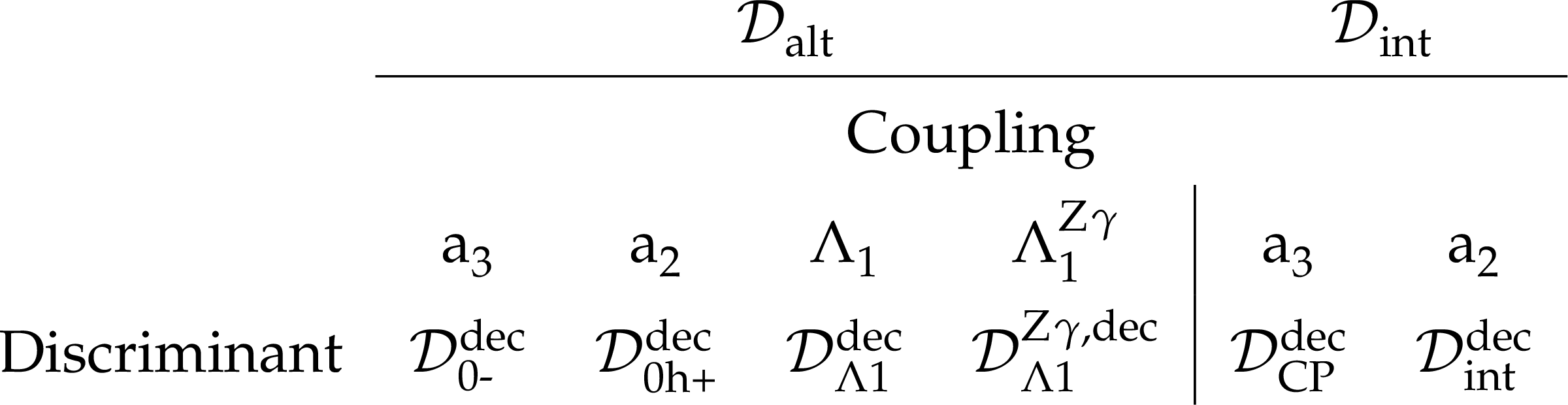
png pdf |
Table 3:
Matrix element kinematic discriminants considered in the analysis. Some discriminants have a special label to identify the targeted Higgs boson property rather than the name of the coupling. $ {\mathcal D}^{\text{dec}}_{\text{0-}} $ is sensitive to a CP-odd Higgs boson, $ {\mathcal D}^{\text{dec}}_{\text{CP}} $ is the observable sensitive to the CP-mixing, and $ {\mathcal D}^{\text{dec}}_{\text{0h+}} $ is sensitive to heavy CP-even Higgs boson. |
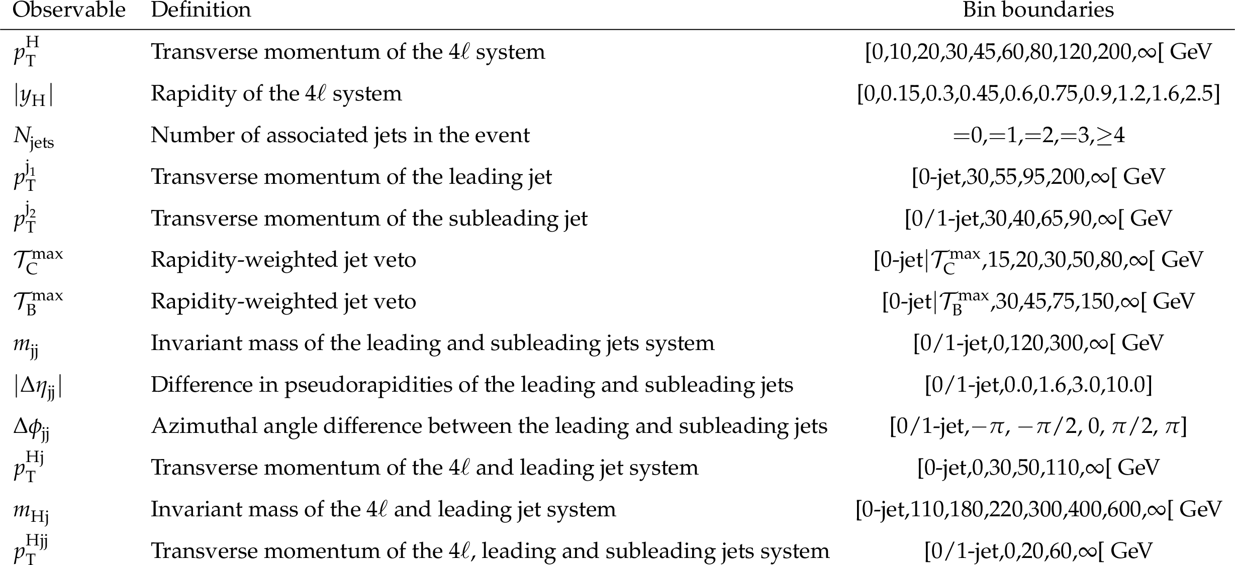
png pdf |
Table 4:
Bin boundaries for one-dimensional observables targeting the H boson production. |
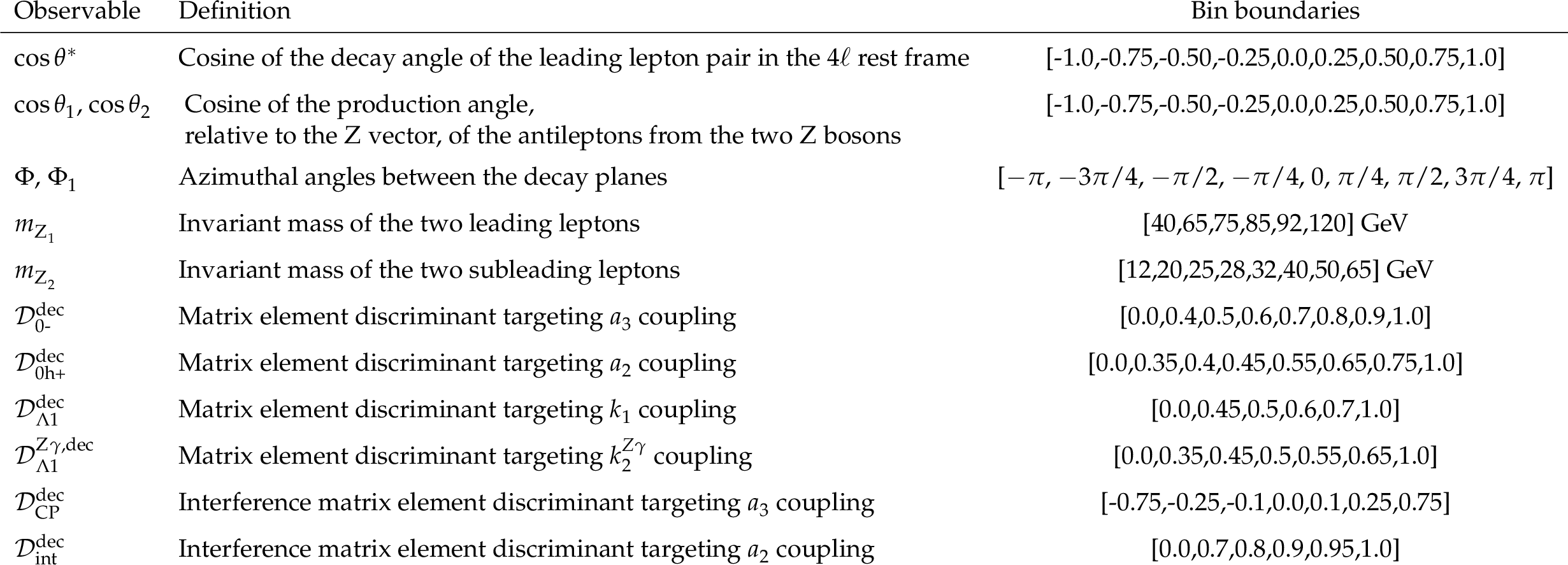
png pdf |
Table 5:
Bin boundaries for one-dimensional observables targeting the $ \mathrm{H}\to\mathrm{Z}\mathrm{Z}\to4\ell $ decay. |
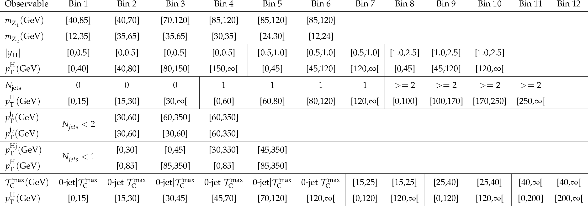
png pdf |
Table 6:
Double-differential observables with their corresponding bin boundaries. |
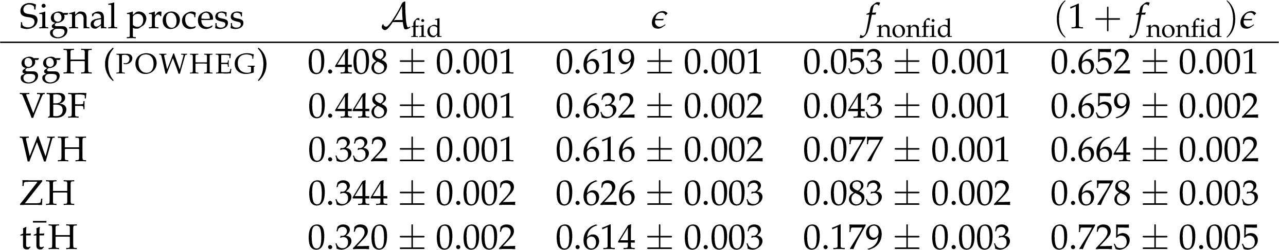
png pdf |
Table 7:
Summary of the inputs to the maximum likelihood based unfolding. The fraction of signal events within the fiducial phase space (acceptance $ \mathcal{A}_{\text{fid}} $), the reconstruction efficiency ($ \epsilon $) in the fiducial phase space, and the ratio of the number of reconstructed events outside the fiducial phase space to that of the ones inside the fiducial phase space ($ f_{\text{nonfid}} $) are quoted for each production mechanism for $ m_{\mathrm{H}}= $ 125.38 GeV. The last column shows the value of $ (1+f_{\text{nonfid}})\epsilon $, which regulates the signal yield for a given fiducial cross section. All values are shown with their statistical uncertainty. The values for the ggH production mode are obtained using the POWHEG generator. |
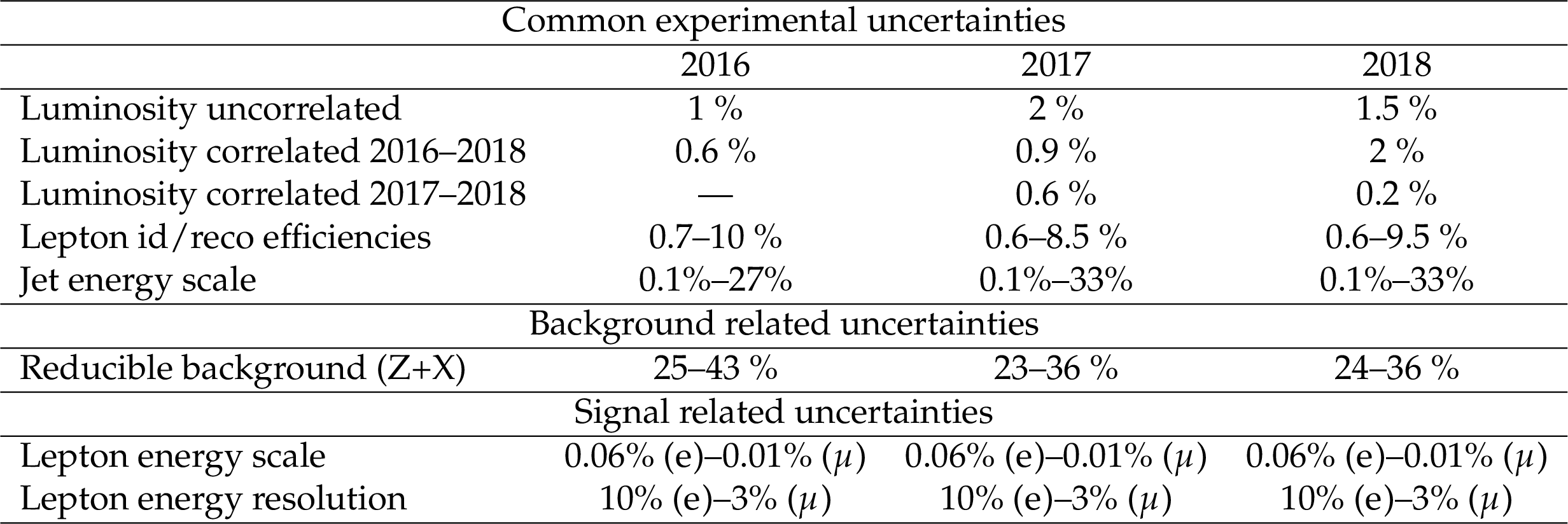
png pdf |
Table 8:
Summary of the experimental systematic uncertainties. |
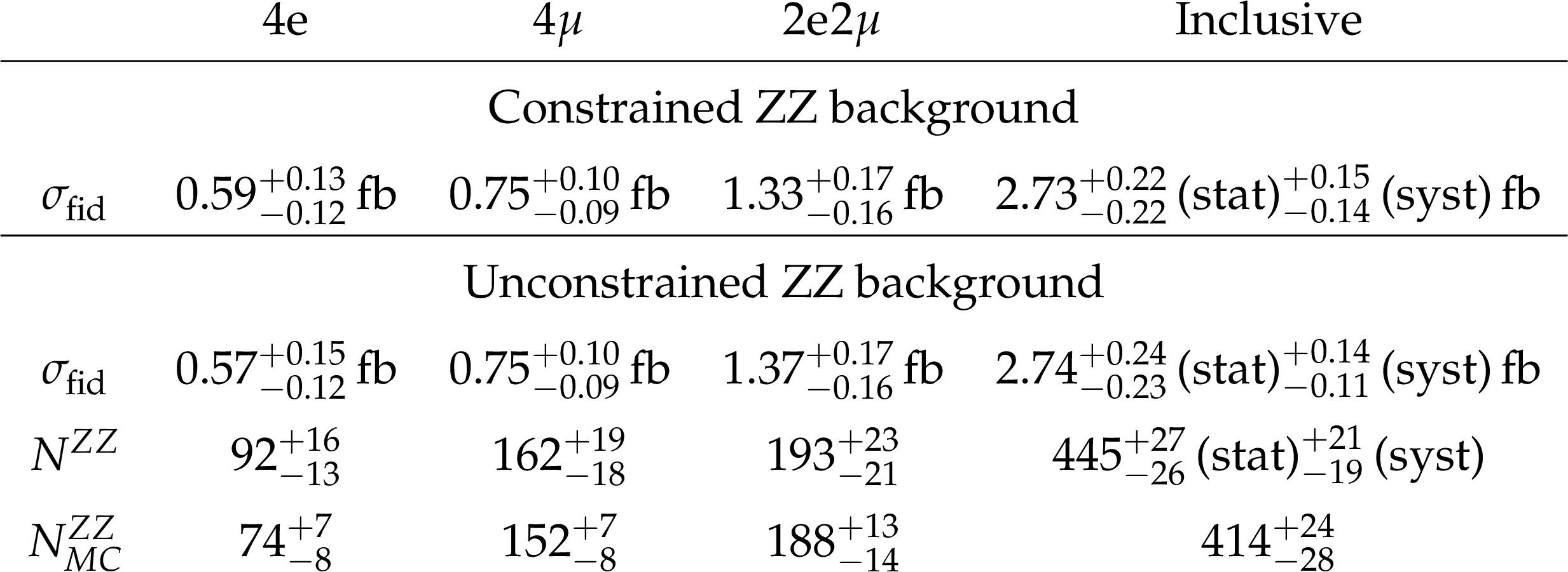
png pdf |
Table 9:
Measured inclusive fiducial cross section and $ \pm $ 1 standard deviation uncertainties for the various final states at $ m_{\mathrm{H}}= $ 125.38 GeV. The upper row summarizes the results obtained when the irreducible background normalization is constrained to the SM expectation and theoretical uncertainty, while the lower section present the results from a fit with the ZZ normalization treated as an unconstrained parameter. The first row presents the fiducial cross section, the middle row the ZZ background normalization extracted from the fit, and the bottom row the ZZ estimation from MC. The uncertainties on $ N^{ZZ}_{MC} $ are the pre-fit uncertainties summing the statistical and systematic uncertainty. |
| Summary |
| This paper presents a comprehensive characterization of the H $\to$ ZZ $\to$ 4$\ell$ decay channel via the measurement of fiducial differential cross sections as functions of several kinematic observables. The H boson production is characterized via measurements of differential cross sections in bins of $ p_{\mathrm{T}}^\mathrm{H} $ and $ |y_\text{\mathrm{H}}| $, the $ p_{\mathrm{T}} $ of the leading and subleading jets and observables of the dijet system, when associated with jets. For the first time, fiducial cross sections are measured in bins of the seven kinematic observables that completely define the four-lepton decay: the invariant mass of the two Z bosons and the five angles that describe the fermions kinematical properties and the production and decay planes. Differential cross sections are also measured for the first time in bins of six matrix element kinematic discriminants sensitive to various anomalous couplings of the H boson to vector bosons. The dynamical evolution of the renormalization and factorization scales, and resummation effects are probed by measuring cross sections in bins of rapidity-weighted jet vetoes, and in bins of observables of the H plus jets system. An extensive set of double-differential measurements is presented, providing a complete coverage of the phase space under study. The $ \mathrm{H}\to\mathrm{Z}\mathrm{Z}\to4\ell $ inclusive fiducial cross section is $ \sigma_{{\text{fid}}}= $ 2.73 $ \pm $ 0.26 fb $= $ 2.73 $ \pm $ 0.22 (stat) $ \pm $ 0.15 (syst) fb, in agreement with the SM expectation of 2.86 $ \pm $ 0.15 fb. The measurement of the fiducial cross section in differential bins of $ p_{\mathrm{T}}^\mathrm{H} $ is used to set constraints on the trilinear self-coupling of the H boson, with an observed (expected) limit of $ -$5.4 ($-$7.6) $ < \kappa_\lambda < $ 14.9 (17.7) at the 95% CL. Finally, constraints on the modifiers of H boson couplings to b and c quarks ($ \kappa_\mathrm{b} $ and $ \kappa_\mathrm{c} $) are also determined with an observed (expected) limit of $ -$1.1 ($-$1.3) $ < \kappa_\mathrm{b} < $ 1.1 (1.2) and $ -$5.3 ($-$5.7) $ < \kappa_\mathrm{c} < $ 5.2 (5.7) at the 95% CL. All results are consistent with the SM predictions for the $ \mathrm{H}\to\mathrm{Z}\mathrm{Z}\to4\ell $ decay channel in the considered fiducial phase space. |
| References | ||||
| 1 | ATLAS Collaboration | Observation of a new particle in the search for the standard model Higgs boson with the ATLAS detector at the LHC | PLB 716 (2012) 1 | 1207.7214 |
| 2 | CMS Collaboration | Observation of a new boson at a mass of 125 GeV with the CMS experiment at the LHC | PLB 716 (2012) 30 | CMS-HIG-12-028 1207.7235 |
| 3 | CMS Collaboration | Observation of a new boson with mass near 125 GeV in pp collisions at $ \sqrt{s} = $ 7 and 8 TeV | JHEP 06 (2013) 081 | CMS-HIG-12-036 1303.4571 |
| 4 | F. Englert and R. Brout | Broken symmetry and the mass of gauge vector mesons | PRL 13 (1964) 321 | |
| 5 | P. W. Higgs | Broken symmetries, massless particles and gauge fields | PL 12 (1964) 132 | |
| 6 | P. W. Higgs | Broken symmetries and the masses of gauge bosons | PRL 13 (1964) 508 | |
| 7 | G. S. Guralnik, C. R. Hagen, and T. W. B. Kibble | Global conservation laws and massless particles | PRL 13 (1964) 585 | |
| 8 | P. W. Higgs | Spontaneous symmetry breakdown without massless bosons | PR 145 (1966) 1156 | |
| 9 | T. W. B. Kibble | Symmetry breaking in nonabelian gauge theories | PR 155 (1967) 1554 | |
| 10 | ATLAS Collaboration | Measurements of the Higgs boson production and decay rates and coupling strengths using pp collision data at $ \sqrt{s}= $ 7 and 8 TeV in the ATLAS experiment | EPJC 76 (2016) 6 | 1507.04548 |
| 11 | CMS Collaboration | Precise determination of the mass of the Higgs boson and tests of compatibility of its couplings with the standard model predictions using proton collisions at 7 and 8 TeV | EPJC 75 (2015) 212 | CMS-HIG-14-009 1412.8662 |
| 12 | ATLAS and CMS Collaborations | Combined measurement of the Higgs boson mass in pp collisions at $ \sqrt{s}= $ 7 and 8 TeV with the ATLAS and CMS experiments | PRL 114 (2015) 191803 | 1503.07589 |
| 13 | ATLAS and CMS Collaborations | Measurements of the Higgs boson production and decay rates and constraints on its couplings from a combined ATLAS and CMS analysis of the LHC pp collision data at $ \sqrt{s}= $ 7 and 8 TeV | JHEP 08 (2016) 45 | 1606.02266 |
| 14 | ATLAS Collaboration | Measurements of Higgs boson production and couplings in the four-lepton channel in pp collisions at center-of-mass energies of 7 and 8 TeV with the ATLAS detector | PRD 91 (2015) 012006 | 1408.5191 |
| 15 | CMS Collaboration | Measurement of the properties of a Higgs boson in the four-lepton final state | PRD 89 (2014) 092007 | CMS-HIG-13-002 1312.5353 |
| 16 | CMS Collaboration | Study of the mass and spin-parity of the Higgs boson candidate via its decays to Z boson pairs | PRL 110 (2013) 081803 | CMS-HIG-12-041 1212.6639 |
| 17 | CMS Collaboration | Constraints on the spin-parity and anomalous HVV couplings of the Higgs boson in proton collisions at 7 and 8 TeV | PRD 92 (2015) 012004 | CMS-HIG-14-018 1411.3441 |
| 18 | CMS Collaboration | Measurements of properties of the Higgs boson decaying into the four-lepton final state in pp collisions at $ \sqrt{s}= $ 13 TeV | JHEP 11 (2017) 047 | CMS-HIG-16-041 1706.09936 |
| 19 | ATLAS Collaboration | Measurement of the Higgs boson coupling properties in the $ H\rightarrow ZZ^{*} \rightarrow 4\ell $ decay channel at $ \sqrt{s} = $ 13 TeV with the ATLAS detector | JHEP 03 (2018) 095 | 1712.02304 |
| 20 | CMS Collaboration | Constraints on the Higgs boson width from off-shell production and decay to Z-boson pairs | PLB 736 (2014) 64 | CMS-HIG-14-002 1405.3455 |
| 21 | CMS Collaboration | Limits on the Higgs boson lifetime and width from its decay to four charged leptons | PRD 92 (2015) 072010 | CMS-HIG-14-036 1507.06656 |
| 22 | ATLAS Collaboration | Constraints on the off-shell Higgs boson signal strength in the high-mass ZZ and WW final states with the ATLAS detector | EPJC 75 (2015) 335 | 1503.01060 |
| 23 | ATLAS Collaboration | Constraints on off-shell Higgs boson production and the Higgs boson total width in ZZ $\to$ 4$\ell $ and ZZ $\to$ 2$\ell$2$\nu $ final states with the ATLAS detector | PLB 786 (2018) 223 | 1808.01191 |
| 24 | ATLAS Collaboration | Fiducial and differential cross sections of Higgs boson production measured in the four-lepton decay channel in pp collisions at $ \sqrt{s}= $ 8 TeV with the ATLAS detector | PLB 738 (2014) 234 | 1408.3226 |
| 25 | CMS Collaboration | Measurement of differential and integrated fiducial cross sections for Higgs boson production in the four-lepton decay channel in pp collisions at $ \sqrt{s}= $ 7 and 8 TeV | JHEP 04 (2016) 005 | CMS-HIG-14-028 1512.08377 |
| 26 | ATLAS Collaboration | Measurement of inclusive and differential cross sections in the H $\rightarrow $ ZZ* $ \rightarrow $ 4$\ell $ decay channel in pp collisions at $ \sqrt{s}= $ 13 TeV with the ATLAS detector | JHEP 10 (2017) 132 | 1708.02810 |
| 27 | ATLAS Collaboration | Higgs boson production cross-section measurements and their EFT interpretation in the 4$ \ell $ decay channel at $ \sqrt{s}= $ 13 TeV with the ATLAS detector | EPJC 80 (2020) 957 | 2004.0344 |
| 28 | ATLAS Collaboration | Measurements of the Higgs boson inclusive and differential fiducial cross sections in the 4$ \ell $ decay channel at $ \sqrt{s}= $ 13 TeV | EPJC 80 (2020) 941 | 2004.03969 |
| 29 | CMS Collaboration | Constraints on anomalous Higgs boson couplings using production and decay information in the four-lepton final state | PLB 775 (2017) 1 | CMS-HIG-17-011 1707.00541 |
| 30 | CMS Collaboration | Measurements of the Higgs boson width and anomalous HVV couplings from on-shell and off-shell production in the four-lepton final state | PRD 99 (2019) 112003 | CMS-HIG-18-002 1901.00174 |
| 31 | CMS Collaboration | Constraints on anomalous Higgs boson couplings to vector bosons and fermions in its production and decay using the four-lepton final state | PRD 104 (2021) 052004 | CMS-HIG-19-009 2104.12152 |
| 32 | CMS Collaboration | A measurement of the Higgs boson mass in the diphoton decay channel | PLB 805 (2020) 135425 | CMS-HIG-19-004 2002.06398 |
| 33 | CMS Collaboration | Measurement of the Higgs boson width and evidence of its off-shell contributions to ZZ production | Nature Phys. 18 (2022) 1329 | CMS-HIG-21-013 2202.06923 |
| 34 | LHC Higgs Cross Section Working Group | Handbook of LHC Higgs Cross Sections: 4. Deciphering the Nature of the Higgs Sector | technical report, 2016 link |
1610.07922 |
| 35 | CMS Collaboration | Measurements of production cross sections of the Higgs boson in the four-lepton final state in proton-proton collisions at $ \sqrt{s} = $ 13 TeV | EPJC 81 (2021) 488 | CMS-HIG-19-001 2103.04956 |
| 36 | ATLAS Collaboration | Measurement of the properties of Higgs boson production at $ \sqrt{s} = $ 13 TeV in the $ H\to\gamma\gamma $ channel using 139 fb$ ^{-1} $ of pp collision data with the ATLAS experiment | Submitted to JHEP, 2022 | 2207.00348 |
| 37 | CMS Collaboration | Measurements of Higgs boson production cross sections and couplings in the diphoton decay channel at $ \sqrt{s} = $ 13 TeV | JHEP 07 (2021) 027 | CMS-HIG-19-015 2103.06956 |
| 38 | ATLAS Collaboration | Measurements of Higgs boson production by gluon-gluon fusion and vector-boson fusion using $ H\rightarrow W W^* \rightarrow e\nu \mu\nu $ decays in pp collisions at $ \sqrt{s}= $ 13 TeV with the ATLAS detector | Submitted to Phys. Rev. D, 2022 | 2207.00338 |
| 39 | CMS Collaboration | Measurements of the Higgs boson production cross section and couplings in the W boson pair decay channel in proton-proton collisions at $ \sqrt{s} = $ 13 TeV | Submitted to Eur. Phys. J. C, 2022 | CMS-HIG-20-013 2206.09466 |
| 40 | ATLAS Collaboration | Measurements of WH and ZH production in the H $ \rightarrow $b\bar{b} $ decay channel in pp collisions at 13 TeV with the ATLAS detector | EPJC 81 (2021) 178 | 2007.02873 |
| 41 | ATLAS Collaboration | Measurements of Higgs boson production cross-sections in the $ H\to\tau^{+}\tau^{-} $ decay channel in pp collisions at $ \sqrt{s}= $ 13 TeV with the ATLAS detector | JHEP 08 (2022) 175 | 2201.08269 |
| 42 | CMS Collaboration | Measurements of Higgs boson production in the decay channel with a pair of $ \tau $ leptons in proton-proton collisions at $ \sqrt{s}= $ 13 TeV | Submitted toEur. Phys. J. C, 2022 | CMS-HIG-19-010 2204.12957 |
| 43 | ATLAS Collaboration | A detailed map of Higgs boson interactions by the ATLAS experiment ten years after the discovery | Nature Phys. 607 (2022) 52 | 2207.00092 |
| 44 | CMS Collaboration | A portrait of the Higgs boson by the CMS experiment ten years after the discovery | Nature 607 (2022) 10 | CMS-HIG-22-001 2207.00043 |
| 45 | ATLAS Collaboration | Measurements of the Higgs boson inclusive and differential fiducial cross-sections in the diphoton decay channel with pp collisions at $ \sqrt{s} = $ 13 TeV with the ATLAS detector | JHEP 08 (2022) 027 | 2202.00487 |
| 46 | CMS Collaboration | Measurement of the Higgs boson inclusive and differential fiducial production cross sections in the diphoton decay channel with pp collisions at $ \sqrt{s}= $ 13 TeV | Submitted to JHEP, 2022 | CMS-HIG-19-016 2208.12279 |
| 47 | ATLAS Collaboration | Measurements of differential cross sections of Higgs boson production through gluon fusion in the H $\to$ WW* $\to$ e$\nu\mu\nu $ final state at $ \sqrt{s} = $ 13 TeV with the ATLAS detector | Submitted toEur. Phys. J. C, 2023 | 2301.06822 |
| 48 | ATLAS Collaboration | Fiducial and differential cross-section measurements for the vector-boson-fusion production of the Higgs boson in the H $ \rightarrow $ WW* $\rightarrow $ e$\nu\mu\nu $ decay channel at 13 TeV with the ATLAS detector | Submitted to Phys. Rev. D, 2023 | 2304.03053 |
| 49 | CMS Collaboration | Measurement of the inclusive and differential Higgs boson production cross sections in the leptonic WW decay mode at $ \sqrt{s} = $ 13 TeV | JHEP 03 (2021) 003 | CMS-HIG-19-002 2007.01984 |
| 50 | CMS Collaboration | Measurement of the inclusive and differential Higgs boson production cross sections in the decay mode to a pair of $ \tau $ leptons in pp collisions at $ \sqrt{s} = $ 13 TeV | PRL 128 (2022) 081805 | CMS-HIG-20-015 2107.11486 |
| 51 | ATLAS Collaboration | Measurement of the total and differential Higgs boson production cross-sections at $ \sqrt{s} = $ 13 TeV with the ATLAS detector by combining the H $\rightarrow $ ZZ* $ \rightarrow $ 4$\ell $ and H $ \rightarrow \gamma \gamma $ decay channels | Submitted to JHEP, 2022 | 2207.08615 |
| 52 | CMS Collaboration | Measurement and interpretation of differential cross sections for Higgs boson production at $ \sqrt{s} = $ 13 TeV | PLB 792 (2019) 369 | CMS-HIG-17-028 1812.06504 |
| 53 | CMS Collaboration | Performance of the CMS Level-1 trigger in proton-proton collisions at $ \sqrt{s} = $ 13 TeV | JINST 15 (2020) P10017 | CMS-TRG-17-001 2006.10165 |
| 54 | CMS Collaboration | The CMS trigger system | JINST 12 (2017) P01020 | CMS-TRG-12-001 1609.02366 |
| 55 | CMS Collaboration | Technical proposal for the phase-II upgrade of the compact muon solenoid | CMS Technical proposal CERN-LHCC-2015-010, CMS-TDR-15-02, 2015 CDS |
|
| 56 | CMS Collaboration | Electron and photon reconstruction and identification with the CMS experiment at the CERN LHC | JINST 16 (2021) P05014 | CMS-EGM-17-001 2012.06888 |
| 57 | CMS Collaboration | ECAL 2016 refined calibration and Run 2 summary plots | CMS Detector Performance Summary CMS-DP-2020-021, 2020 CDS |
|
| 58 | CMS Collaboration | Performance of the CMS muon detector and muon reconstruction with proton-proton collisions at $ \sqrt{s}= $ 13 TeV | JINST 13 (2018) P06015 | CMS-MUO-16-001 1804.04528 |
| 59 | CMS Collaboration | The CMS experiment at the CERN LHC | JINST 3 (2008) S08004 | |
| 60 | CMS Collaboration | Precision luminosity measurement in proton-proton collisions at $ \sqrt{s} = $ 13 TeV in 2015 and 2016 at CMS | EPJC 81 (2021) 800 | CMS-LUM-17-003 2104.01927 |
| 61 | CMS Collaboration | CMS luminosity measurement for the 2017 data-taking period at $ \sqrt{s} = $ 13 TeV | CMS Physics Analysis Summary, 2018 CMS-PAS-LUM-17-004 |
CMS-PAS-LUM-17-004 |
| 62 | CMS Collaboration | CMS luminosity measurement for the 2018 data-taking period at $ \sqrt{s} = $ 13 TeV | CMS Physics Analysis Summary, 2019 CMS-PAS-LUM-18-002 |
CMS-PAS-LUM-18-002 |
| 63 | CMS Collaboration | Measurement of the Inclusive W and Z Production Cross Sections in pp Collisions at $ \sqrt{s}= $ 7 TeV | JHEP 10 (2011) 132 | CMS-EWK-10-005 1107.4789 |
| 64 | P. Nason | A new method for combining NLO QCD with shower Monte Carlo algorithms | JHEP 11 (2004) 040 | hep-ph/0409146 |
| 65 | S. Frixione, P. Nason, and C. Oleari | Matching NLO QCD computations with parton shower simulations: the POWHEG method | JHEP 11 (2007) 070 | 0709.2092 |
| 66 | S. Alioli, P. Nason, C. Oleari, and E. Re | A general framework for implementing NLO calculations in shower Monte Carlo programs: the POWHEG BOX | JHEP 06 (2010) 043 | 1002.2581 |
| 67 | S. Alioli, P. Nason, C. Oleari, and E. Re | NLO Higgs boson production via gluon fusion matched with shower in POWHEG | JHEP 04 (2009) 002 | 0812.0578 |
| 68 | P. Nason and C. Oleari | NLO Higgs boson production via vector-boson fusion matched with shower in POWHEG | JHEP 02 (2010) 037 | 0911.5299 |
| 69 | G. Luisoni, P. Nason, C. Oleari, and F. Tramontano | HW$ ^{\pm} $/HZ + 0 and 1 jet at NLO with the POWHEG BOX interfaced to GoSam and their merging within MiNLO | JHEP 10 (2013) 1 | 1306.2542 |
| 70 | H. B. Hartanto, B. Jager, L. Reina, and D. Wackeroth | Higgs boson production in association with top quarks in the POWHEG BOX | PRD 91 (2015) 094003 | 1501.04498 |
| 71 | K. Hamilton, P. Nason, E. Re, and G. Zanderighi | NNLOPS simulation of Higgs boson production | JHEP 10 (2013) 222 | 1309.0017 |
| 72 | Y. Gao et al. | Spin determination of single-produced resonances at hadron colliders | PRD 81 (2010) 075022 | 1001.3396 |
| 73 | S. Bolognesi et al. | On the spin and parity of a single-produced resonance at the LHC | PRD 86 (2012) 095031 | 1208.4018 |
| 74 | I. Anderson et al. | Constraining anomalous HVV interactions at proton and lepton colliders | PRD 89 (2014) 035007 | 1309.4819 |
| 75 | A. V. Gritsan, R. Röntsch, M. Schulze, and M. Xiao | Constraining anomalous Higgs boson couplings to the heavy flavor fermions using matrix element techniques | PRD 94 (2016) 055023 | 1606.03107 |
| 76 | A. V. Gritsan et al. | New features in the JHU generator framework: constraining Higgs boson properties from on-shell and off-shell production | PRD 102 (2020) 056022 | 2002.09888 |
| 77 | M. Wiesemann et al. | Higgs production in association with bottom quarks | JHEP 02 (2015) 132 | 1409.5301 |
| 78 | C. Anastasiou et al. | Higgs boson gluon-fusion production in QCD at three loops | PRL 114 (2015) 212001 | 1503.06056 |
| 79 | C. Anastasiou et al. | High precision determination of the gluon fusion Higgs boson cross-section at the LHC | JHEP 05 (2016) 58 | 1602.00695 |
| 80 | M. Ciccolini, A. Denner, and S. Dittmaier | Strong and electroweak corrections to the production of a Higgs boson+2 jets via weak interactions at the Large Hadron Collider | PRL 99 (2007) 161803 | 0707.0381 |
| 81 | M. Ciccolini, A. Denner, and S. Dittmaier | Electroweak and QCD corrections to Higgs production via vector-boson fusion at the LHC | PRD 77 (2008) 013002 | 0710.4749 |
| 82 | P. Bolzoni, F. Maltoni, S.-O. Moch, and M. Zaro | Higgs production via vector-boson fusion at NNLO in QCD | PRL 105 (2010) 011801 | 1003.4451 |
| 83 | P. Bolzoni, F. Maltoni, S.-O. Moch, and M. Zaro | Vector boson fusion at next-to-next-to-leading order in QCD: Standard model Higgs boson and beyond | PRD 85 (2012) 035002 | 1109.3717 |
| 84 | O. Brein, A. Djouadi, and R. Harlander | NNLO QCD corrections to the Higgs-strahlung processes at hadron colliders | PLB 579 (2004) 149 | hep-ph/0307206 |
| 85 | M. L. Ciccolini, S. Dittmaier, and M. Kr ä mer | Electroweak radiative corrections to associated WH and ZH production at hadron colliders | PRD 68 (2003) 073003 | hep-ph/0306234 |
| 86 | W. Beenakker et al. | Higgs radiation off top quarks at the Tevatron and the LHC | PRL 87 (2001) 201805 | hep-ph/0107081 |
| 87 | W. Beenakker et al. | NLO QCD corrections to $ {\mathrm{t}\overline{\mathrm{t}}} $ H production in hadron collisions. | NPB 653 (2003) 151 | hep-ph/0211352 |
| 88 | S. Dawson, L. H. Orr, L. Reina, and D. Wackeroth | Associated top quark Higgs boson production at the LHC | PRD 67 (2003) 071503 | hep-ph/0211438 |
| 89 | S. Dawson et al. | Associated Higgs production with top quarks at the Large Hadron Collider: NLO QCD corrections | PRD 68 (2003) 034022 | hep-ph/0305087 |
| 90 | Z. Yu et al. | QCD NLO and EW NLO corrections to $ t\bar{t}H $ production with top quark decays at hadron collider | PLB 738 (2014) 1 | 1407.1110 |
| 91 | S. S. Frixione et al. | Weak corrections to Higgs hadroproduction in association with a top-quark pair | JHEP 09 (2014) 65 | 1407.0823 |
| 92 | F. Demartin, F. Maltoni, K. Mawatari, and M. Zaro | Higgs production in association with a single top quark at the LHC | EPJC 75 (2015) 267 | 1504.0611 |
| 93 | F. Demartin et al. | tWH associated production at the LHC | EPJC 77 (2017) 34 | 1607.05862 |
| 94 | A. Denner et al. | Standard model Higgs-boson branching ratios with uncertainties | EPJC 71 (2011) 1753 | 1107.5909 |
| 95 | A. Djouadi, J. Kalinowski, and M. Spira | HDECAY: A program for Higgs boson decays in the standard model and its supersymmetric extension | Comput. Phys. Commun. 108 (1998) 56 | hep-ph/9704448 |
| 96 | A. Djouadi, J. Kalinowski, M. Muhlleitner, and M. Spira | An update of the program HDECAY | in Les Houches workshop on TeV colliders 2009: The tools and Monte Carlo working group summary report (2010) | 1003.1643 |
| 97 | A. Bredenstein, A. Denner, S. Dittmaier, and M. M. Weber | Precise predictions for the Higgs-boson decay H $ \rightarrow $ WW/ZZ $ \rightarrow $ 4 leptons | PRD 74 (2006) 013004 | hep-ph/0604011 |
| 98 | A. Bredenstein, A. Denner, S. Dittmaier, and M. M. Weber | Radiative corrections to the semileptonic and hadronic Higgs-boson decays H $ \rightarrow $ WW/ZZ $ \rightarrow $ 4 fermions | JHEP 02 (2007) 80 | hep-ph/0611234 |
| 99 | S. Boselli et al. | Higgs boson decay into four leptons at NLOPS electroweak accuracy | JHEP 06 (2015) 23 | 1503.07394 |
| 100 | S. Actis, G. Passarino, C. Sturm, and S. Uccirati | NNLO computational techniques: the cases H $ \to \gamma \gamma $ and H $ \to$ gg | NPB 811 (2009) 182 | 0809.3667 |
| 101 | T. Melia, P. Nason, R. Rontsch, and G. Zanderighi | W$ ^{+} $W$ ^{-} $, WZ and ZZ production in the POWHEG BOX | JHEP 11 (2011) 078 | 1107.5051 |
| 102 | J. M. Campbell and R. K. Ellis | MCFM for the Tevatron and the LHC | Nucl. Phys. Proc. Suppl. 20 (2010) 5 | 1007.3492 |
| 103 | J. M. Campbell, R. K. Ellis, and C. Williams | Vector boson pair production at the LHC | JHEP 07 (2011) 018 | 1105.0020 |
| 104 | J. M. Campbell, R. K. Ellis, and C. Williams | Bounding the Higgs width at the LHC using full analytic results for $ \mathrm{g}\mathrm{g}\to \mathrm{e}^{-}\mathrm{e}^{+} \mu^{-} \mu^{+} $ | JHEP 04 (2014) 060 | 1311.3589 |
| 105 | J. M. Campbell and R. K. Ellis | Higgs constraints from vector boson fusion and scattering | JHEP 04 (2015) 030 | 1502.02990 |
| 106 | T. Sjöstrand et al. | An introduction to PYTHIA 8.2 | Comput. Phys. Commun. 191 (2015) 159 | 1410.3012 |
| 107 | CMS Collaboration | Event generator tunes obtained from underlying event and multiparton scattering measurements | EPJC 76 (2016) 155 | CMS-GEN-14-001 1512.00815 |
| 108 | CMS Collaboration | Extraction and validation of a new set of CMS PYTHIA8 tunes from underlying-event measurements | EPJC 80 (2020) 4 | CMS-GEN-17-001 1903.12179 |
| 109 | NNPDF Collaboration | Parton distributions for the LHC Run II | JHEP 04 (2015) 040 | 1410.8849 |
| 110 | GEANT 4 Collaboration | GEANT 4--a simulation toolkit | NIM A 506 (2003) 250 | |
| 111 | GEANT 4 Collaboration, J. Allison et al. | GEANT 4 developments and applications | IEEE Trans. Nucl. Sci. 53 (2006) 270 | |
| 112 | CMS Collaboration | Particle-flow reconstruction and global event description with the CMS detector | JINST 12 (2017) P10003 | CMS-PRF-14-001 1706.04965 |
| 113 | T. Chen and C. Guestrin | XGBoost: A scalable tree boosting system | technical report, 2016 link |
1603.02754 |
| 114 | CMS Collaboration | Pileup mitigation at CMS in 13 TeV data | JINST 15 (2020) P09018 | CMS-JME-18-001 2003.00503 |
| 115 | M. Cacciari, G. P. Salam, and G. Soyez | The anti-$ k_{\mathrm{T}} $ jet clustering algorithm | JHEP 04 (2008) 063 | 0802.1189 |
| 116 | M. Cacciari, G. P. Salam, and G. Soyez | FastJet user manual | EPJC 72 (2012) 1896 | 1111.6097 |
| 117 | CMS Collaboration | Jet energy scale and resolution in the CMS experiment in pp collisions at 8 TeV | JINST 12 (2017) P02014 | CMS-JME-13-004 1607.03663 |
| 118 | Particle Data Group, P. A. Zyla et al. | Review of particle physics | Prog. Theor. Exp. Phys. 2022 (2022) 083C01 | |
| 119 | S. Gangal, M. Stahlhofen, and F. J. Tackmann | Rapidity-Dependent Jet Vetoes | PRD 91 (2015) 054023 | 1412.4792 |
| 120 | M. Grazzini, S. Kallweit, and D. Rathlev | ZZ production at the LHC: Fiducial cross sections and distributions in NNLO QCD | PLB 750 (2015) 407 | 1507.06257 |
| 121 | A. Bierweiler, T. Kasprzik, and J. H. Kühn | Vector-boson pair production at the LHC to $ \mathcal{O}(\alpha^3) $ accuracy | JHEP 12 (2013) 071 | 1305.5402 |
| 122 | M. Bonvini et al. | Signal-background interference effects in gg $\to$ H $\to$ WW beyond leading order | PRD 88 (2013) 034032 | 1304.3053 |
| 123 | K. Melnikov and M. Dowling | Production of two Z-bosons in gluon fusion in the heavy top quark approximation | PLB 744 (2015) 43 | 1503.01274 |
| 124 | C. S. Li, H. T. Li, D. Y. Shao, and J. Wang | Soft gluon resummation in the signal-background interference process of gg($ \rightarrow $ h$ ^{*} $) $ \rightarrow $ ZZ | JHEP 08 (2015) 065 | 1504.02388 |
| 125 | G. Passarino | Higgs CAT | EPJC 74 (2014) 2866 | 1312.2397 |
| 126 | S. Catani and M. Grazzini | An NNLO subtraction formalism in hadron collisions and its application to Higgs boson production at the LHC | PRL 98 (2007) 222002 | hep-ph/0703012 |
| 127 | M. Grazzini | NNLO predictions for the Higgs boson signal in the H $ \to $ WW $\to \ell\nu\ell\nu $ and H $ \to $ ZZ $\to$ 4$\ell $ decay channels | JHEP 02 (2008) 043 | 0801.3232 |
| 128 | M. Grazzini and H. Sargsyan | Heavy-quark mass effects in Higgs boson production at the LHC | JHEP 09 (2013) 129 | 1306.4581 |
| 129 | T. Skwarnicki | A study of the radiative CASCADE transitions between the Upsilon-Prime and Upsilon resonances | PhD thesis, Cracow, INP, 1986 | |
| 130 | ATLAS Collaboration, CMS Collaboration, and LHC Higgs Combination Group | Procedure for the LHC Higgs boson search combination in Summer 2011 | Technical Report CMS-NOTE-2011-005, ATL-PHYS-PUB-2011-11, 2011 | |
| 131 | G. Cowan, K. Cranmer, E. Gross, and O. Vitells | Asymptotic formulae for likelihood-based tests of new physics | EPJC 71 (2011) 1554 | 1007.1727 |
| 132 | CMS Collaboration | Measurement of differential cross sections for Higgs boson production in the diphoton decay channel in pp collisions at $ \sqrt{s} =$ 8 TeV | EPJC 76 (2016) 13 | CMS-HIG-14-016 1508.07819 |
| 133 | J. Butterworth et al. | PDF4LHC recommendations for LHC Run II | JPG 43 (2016) 023001 | 1510.03865 |
| 134 | ATLAS Collaboration | Electron reconstruction and identification in the ATLAS experiment using the 2015 and 2016 LHC proton-proton collision data at $ \sqrt{s}= $ 13 TeV | EPJC 79 (2019) 639 | 1902.04655 |
| 135 | CMS Collaboration | HEPData record for this analysis | link | |
| 136 | D. de Florian, G. Ferrera, M. Grazzini, and D. Tommasini | Higgs boson production at the LHC: transverse momentum resummation effects in the H $\to \gamma \gamma $, H $\to$ WW \$to \ell\nu\ell\nu $ and H $\to$ ZZ $\to$ 4$\ell $ decay modes | JHEP 06 (2012) 132 | 1203.6321 |
| 137 | G. Degrassi, P. P. Giardino, F. Maltoni, and D. Pagani | Probing the Higgs self coupling via single Higgs production at the LHC | JHEP 12 (2016) 080 | 1607.04251 |
| 138 | F. Maltoni, D. Pagani, A. Shivaji, and X. Zhao | Trilinear Higgs coupling determination via single-Higgs differential measurements at the LHC | EPJC 77 (2017) 887 | 1709.08649 |
| 139 | S. Di Vita et al. | A global view on the Higgs self-coupling | JHEP 09 (2017) 069 | 1704.01953 |
| 140 | ATLAS Collaboration | Constraining the Higgs boson self-coupling from single- and double-Higgs production with the ATLAS detector using pp collisions at $ \sqrt{s}= $ 13 TeV | Submitted to PLB, 2022 | 2211.01216 |
| 141 | LHC Higgs Cross Section Working Group | Handbook of LHC Higgs Cross Sections: 3. Higgs Properties | CERN Report CERN-2013-004, 2013 link |
1307.1347 |
| 142 | F. Bishara, U. Haisch, P. F. Monni, and E. Re | Constraining Light-Quark Yukawa Couplings from Higgs Distributions | PRL 118 (2017) 121801 | 1606.09253 |
|
|
Compact Muon Solenoid LHC, CERN |
|

|

|

|

|

|