

Compact Muon Solenoid
LHC, CERN
| CMS-EXO-22-011 ; CERN-EP-2024-032 | ||
| Search for heavy neutral leptons in final states with electrons, muons, and hadronically decaying tau leptons in proton-proton collisions at $ \sqrt{s} = $ 13 TeV | ||
| CMS Collaboration | ||
| 29 February 2024 | ||
| Submitted to J. High Energy Phys. | ||
| Abstract: A search for heavy neutral leptons (HNLs) of Majorana or Dirac type using proton-proton collision data at $ \sqrt{s} = $ 13 TeV is presented. The data were collected by the CMS experiment at the CERN LHC and correspond to an integrated luminosity of 138 fb$ ^{-1} $. Events with three charged leptons (electrons, muons, and hadronically decaying tau leptons) are selected, corresponding to HNL production in association with a charged lepton and decay of the HNL to two charged leptons and a standard model (SM) neutrino. The search is performed for HNL masses between 10 GeV and 1.5 TeV. No evidence for an HNL signal is observed in data. Upper limits at 95% confidence level are found for the squared coupling strength of the HNL to SM neutrinos, considering exclusive coupling of the HNL to a single SM neutrino generation, for both Majorana and Dirac HNLs. The limits exceed previously achieved experimental constraints for a wide range of HNL masses, and the limits on tau neutrino coupling scenarios with HNL masses above the W boson mass are presented for the first time. | ||
| Links: e-print arXiv:2403.00100 [hep-ex] (PDF) ; CDS record ; inSPIRE record ; CADI line (restricted) ; | ||
| Figures | |

png pdf |
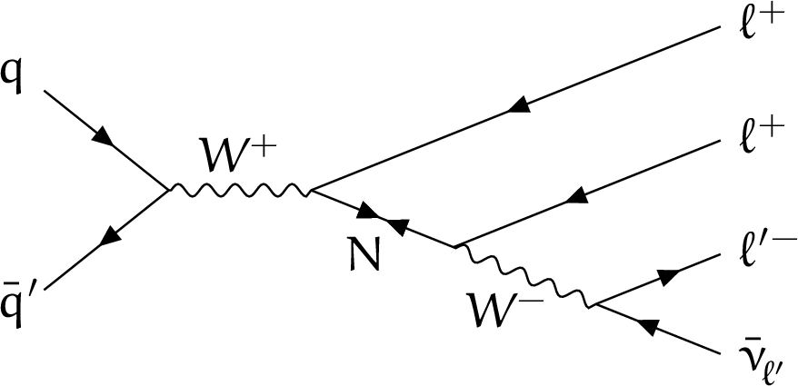
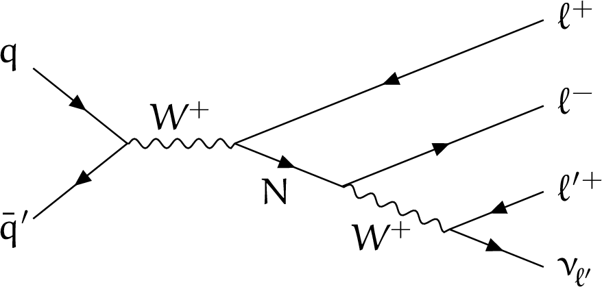
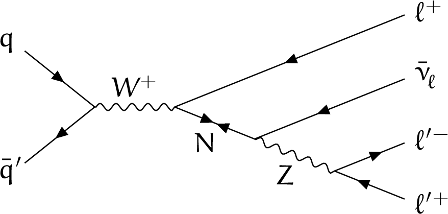
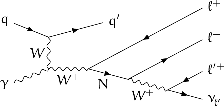
Figure 1:
Examples of Feynman diagrams for production and decay of an HNL (indicated with the symbol $ \mathrm{N} $) resulting in final states with three charged leptons. The production processes DY (upper row and lower left) and VBF (lower right) are shown, with decays mediated by a W boson (upper row and lower right) or a Z boson (lower left). In the left column, HNLs of Majorana type with an LNV decay are shown, whereas the right column has HNLs of Dirac type with an LNC decay. The leptons that couple directly to the HNL (indicated with the symbol $\ell$) are restricted to the SM generation that couples with the HNL, whereas the leptons from the W and Z boson decays (indicated with the symbol $ \ell^\prime $) can be from any SM generation. |
png pdf |
Figure 1-a:
Examples of Feynman diagrams for production and decay of an HNL (indicated with the symbol $ \mathrm{N} $) resulting in final states with three charged leptons. The production processes DY (upper row and lower left) and VBF (lower right) are shown, with decays mediated by a W boson (upper row and lower right) or a Z boson (lower left). In the left column, HNLs of Majorana type with an LNV decay are shown, whereas the right column has HNLs of Dirac type with an LNC decay. The leptons that couple directly to the HNL (indicated with the symbol $\ell$) are restricted to the SM generation that couples with the HNL, whereas the leptons from the W and Z boson decays (indicated with the symbol $ \ell^\prime $) can be from any SM generation. |
png pdf |
Figure 1-b:
Examples of Feynman diagrams for production and decay of an HNL (indicated with the symbol $ \mathrm{N} $) resulting in final states with three charged leptons. The production processes DY (upper row and lower left) and VBF (lower right) are shown, with decays mediated by a W boson (upper row and lower right) or a Z boson (lower left). In the left column, HNLs of Majorana type with an LNV decay are shown, whereas the right column has HNLs of Dirac type with an LNC decay. The leptons that couple directly to the HNL (indicated with the symbol $\ell$) are restricted to the SM generation that couples with the HNL, whereas the leptons from the W and Z boson decays (indicated with the symbol $ \ell^\prime $) can be from any SM generation. |
png pdf |
Figure 1-c:
Examples of Feynman diagrams for production and decay of an HNL (indicated with the symbol $ \mathrm{N} $) resulting in final states with three charged leptons. The production processes DY (upper row and lower left) and VBF (lower right) are shown, with decays mediated by a W boson (upper row and lower right) or a Z boson (lower left). In the left column, HNLs of Majorana type with an LNV decay are shown, whereas the right column has HNLs of Dirac type with an LNC decay. The leptons that couple directly to the HNL (indicated with the symbol $\ell$) are restricted to the SM generation that couples with the HNL, whereas the leptons from the W and Z boson decays (indicated with the symbol $ \ell^\prime $) can be from any SM generation. |
png pdf |
Figure 1-d:
Examples of Feynman diagrams for production and decay of an HNL (indicated with the symbol $ \mathrm{N} $) resulting in final states with three charged leptons. The production processes DY (upper row and lower left) and VBF (lower right) are shown, with decays mediated by a W boson (upper row and lower right) or a Z boson (lower left). In the left column, HNLs of Majorana type with an LNV decay are shown, whereas the right column has HNLs of Dirac type with an LNC decay. The leptons that couple directly to the HNL (indicated with the symbol $\ell$) are restricted to the SM generation that couples with the HNL, whereas the leptons from the W and Z boson decays (indicated with the symbol $ \ell^\prime $) can be from any SM generation. |

png pdf |
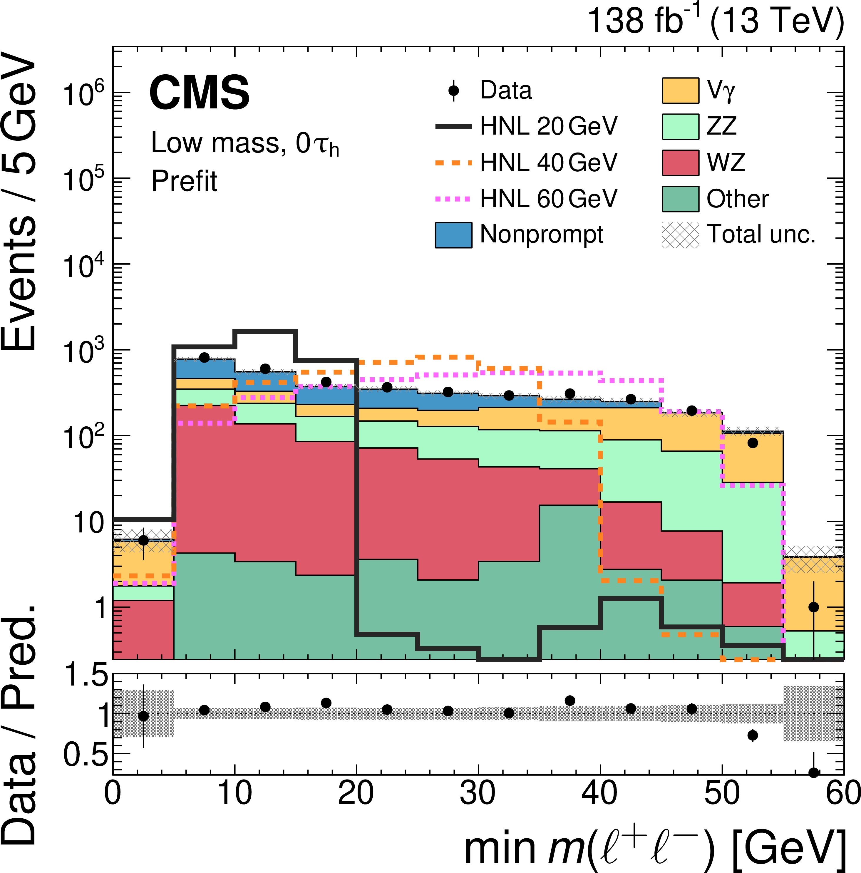
Figure 2:
Comparison of observed (points) and predicted (coloured histograms) distributions in the low-mass selection for the 0$ {\tau}{\mathrm{h}} $ categories combined. Important input variables to the BDT training are shown: $ \min m({\ell}^{+}{\ell}^{-}) $ (upper left), $ m_{\mathrm{T}} $ (upper right), $ \Delta R $ between the two leptons used for $ \min m({\ell}^{+}{\ell}^{-}) $ ($ \Delta R[\min m({\ell}^{+}{\ell}^{-})] $, lower left), $ m(3$\ell$) $ (lower right). The predicted background yields are shown before the fit to the data (``prefit''). The HNL predictions for three different $ m_{\mathrm{N}} $ values with exclusive coupling to tau neutrinos are shown with coloured lines, and are normalized to the total background yield. The vertical bars on the points represent the statistical uncertainties in the data, and the hatched bands the total uncertainties in the predictions. The last bins include the overflow contributions. In the lower panels, the ratios of the event yield in data to the overall sum of the predictions are shown. |
png pdf |
Figure 2-a:
Comparison of observed (points) and predicted (coloured histograms) distributions in the low-mass selection for the 0$ {\tau}{\mathrm{h}} $ categories combined. Important input variables to the BDT training are shown: $ \min m({\ell}^{+}{\ell}^{-}) $ (upper left), $ m_{\mathrm{T}} $ (upper right), $ \Delta R $ between the two leptons used for $ \min m({\ell}^{+}{\ell}^{-}) $ ($ \Delta R[\min m({\ell}^{+}{\ell}^{-})] $, lower left), $ m(3$\ell$) $ (lower right). The predicted background yields are shown before the fit to the data (``prefit''). The HNL predictions for three different $ m_{\mathrm{N}} $ values with exclusive coupling to tau neutrinos are shown with coloured lines, and are normalized to the total background yield. The vertical bars on the points represent the statistical uncertainties in the data, and the hatched bands the total uncertainties in the predictions. The last bins include the overflow contributions. In the lower panels, the ratios of the event yield in data to the overall sum of the predictions are shown. |
png pdf |
Figure 2-b:
Comparison of observed (points) and predicted (coloured histograms) distributions in the low-mass selection for the 0$ {\tau}{\mathrm{h}} $ categories combined. Important input variables to the BDT training are shown: $ \min m({\ell}^{+}{\ell}^{-}) $ (upper left), $ m_{\mathrm{T}} $ (upper right), $ \Delta R $ between the two leptons used for $ \min m({\ell}^{+}{\ell}^{-}) $ ($ \Delta R[\min m({\ell}^{+}{\ell}^{-})] $, lower left), $ m(3$\ell$) $ (lower right). The predicted background yields are shown before the fit to the data (``prefit''). The HNL predictions for three different $ m_{\mathrm{N}} $ values with exclusive coupling to tau neutrinos are shown with coloured lines, and are normalized to the total background yield. The vertical bars on the points represent the statistical uncertainties in the data, and the hatched bands the total uncertainties in the predictions. The last bins include the overflow contributions. In the lower panels, the ratios of the event yield in data to the overall sum of the predictions are shown. |
png pdf |
Figure 2-c:
Comparison of observed (points) and predicted (coloured histograms) distributions in the low-mass selection for the 0$ {\tau}{\mathrm{h}} $ categories combined. Important input variables to the BDT training are shown: $ \min m({\ell}^{+}{\ell}^{-}) $ (upper left), $ m_{\mathrm{T}} $ (upper right), $ \Delta R $ between the two leptons used for $ \min m({\ell}^{+}{\ell}^{-}) $ ($ \Delta R[\min m({\ell}^{+}{\ell}^{-})] $, lower left), $ m(3$\ell$) $ (lower right). The predicted background yields are shown before the fit to the data (``prefit''). The HNL predictions for three different $ m_{\mathrm{N}} $ values with exclusive coupling to tau neutrinos are shown with coloured lines, and are normalized to the total background yield. The vertical bars on the points represent the statistical uncertainties in the data, and the hatched bands the total uncertainties in the predictions. The last bins include the overflow contributions. In the lower panels, the ratios of the event yield in data to the overall sum of the predictions are shown. |
png pdf |
Figure 2-d:
Comparison of observed (points) and predicted (coloured histograms) distributions in the low-mass selection for the 0$ {\tau}{\mathrm{h}} $ categories combined. Important input variables to the BDT training are shown: $ \min m({\ell}^{+}{\ell}^{-}) $ (upper left), $ m_{\mathrm{T}} $ (upper right), $ \Delta R $ between the two leptons used for $ \min m({\ell}^{+}{\ell}^{-}) $ ($ \Delta R[\min m({\ell}^{+}{\ell}^{-})] $, lower left), $ m(3$\ell$) $ (lower right). The predicted background yields are shown before the fit to the data (``prefit''). The HNL predictions for three different $ m_{\mathrm{N}} $ values with exclusive coupling to tau neutrinos are shown with coloured lines, and are normalized to the total background yield. The vertical bars on the points represent the statistical uncertainties in the data, and the hatched bands the total uncertainties in the predictions. The last bins include the overflow contributions. In the lower panels, the ratios of the event yield in data to the overall sum of the predictions are shown. |
png pdf |
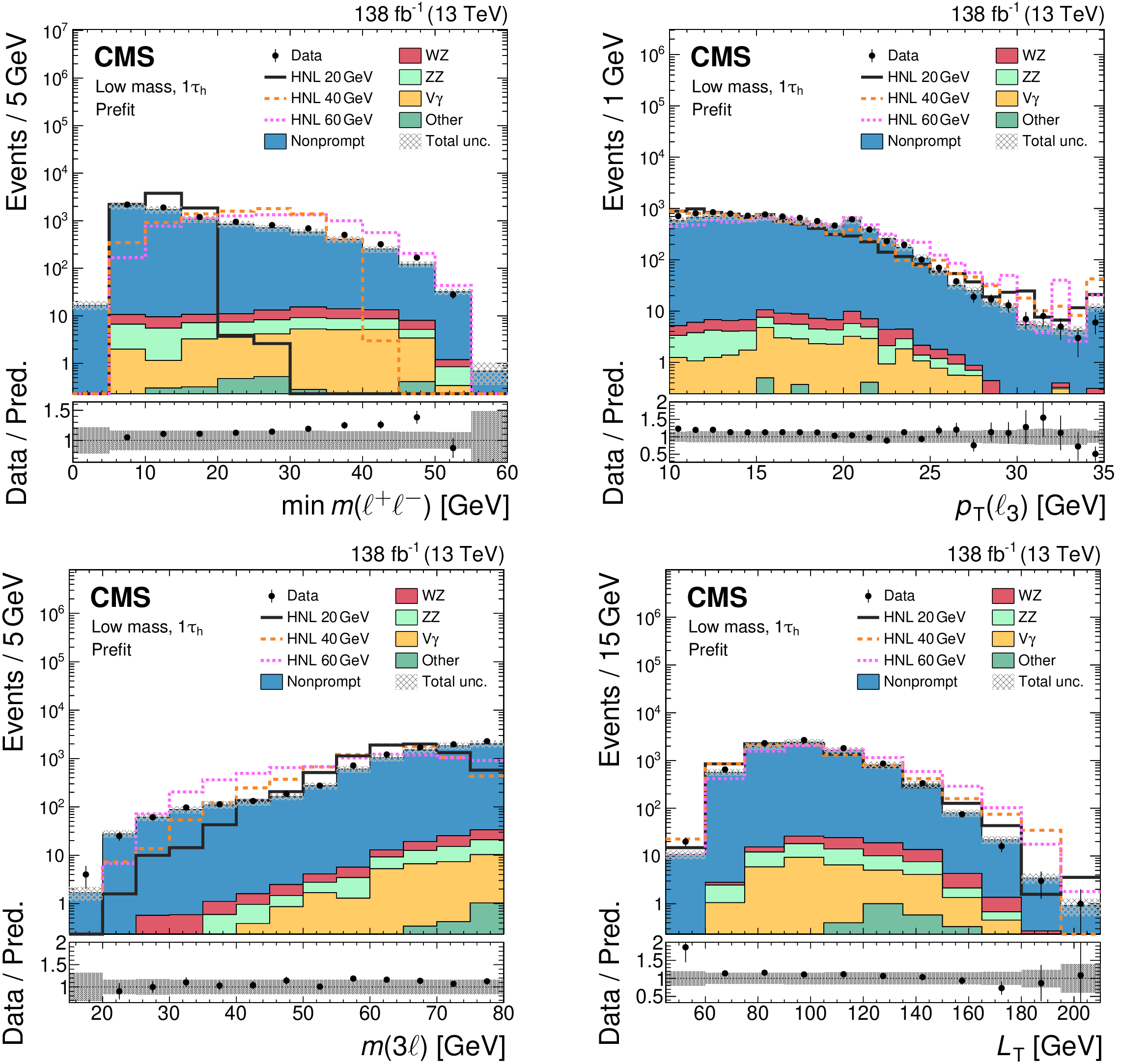
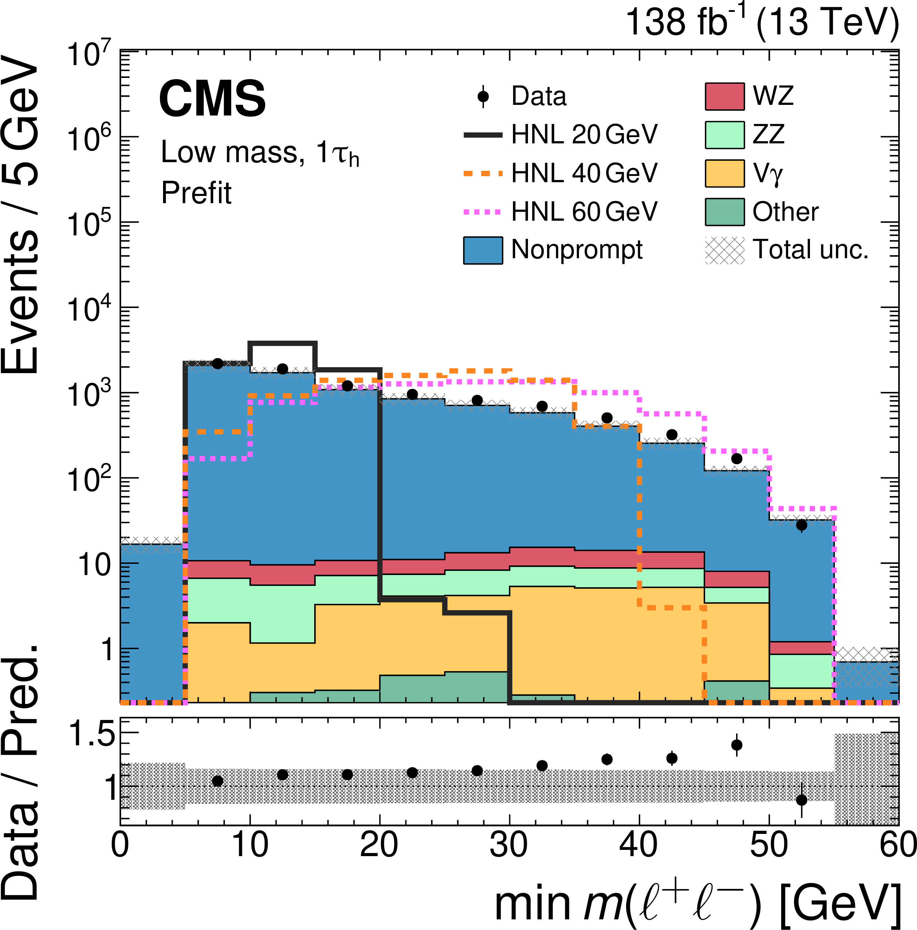
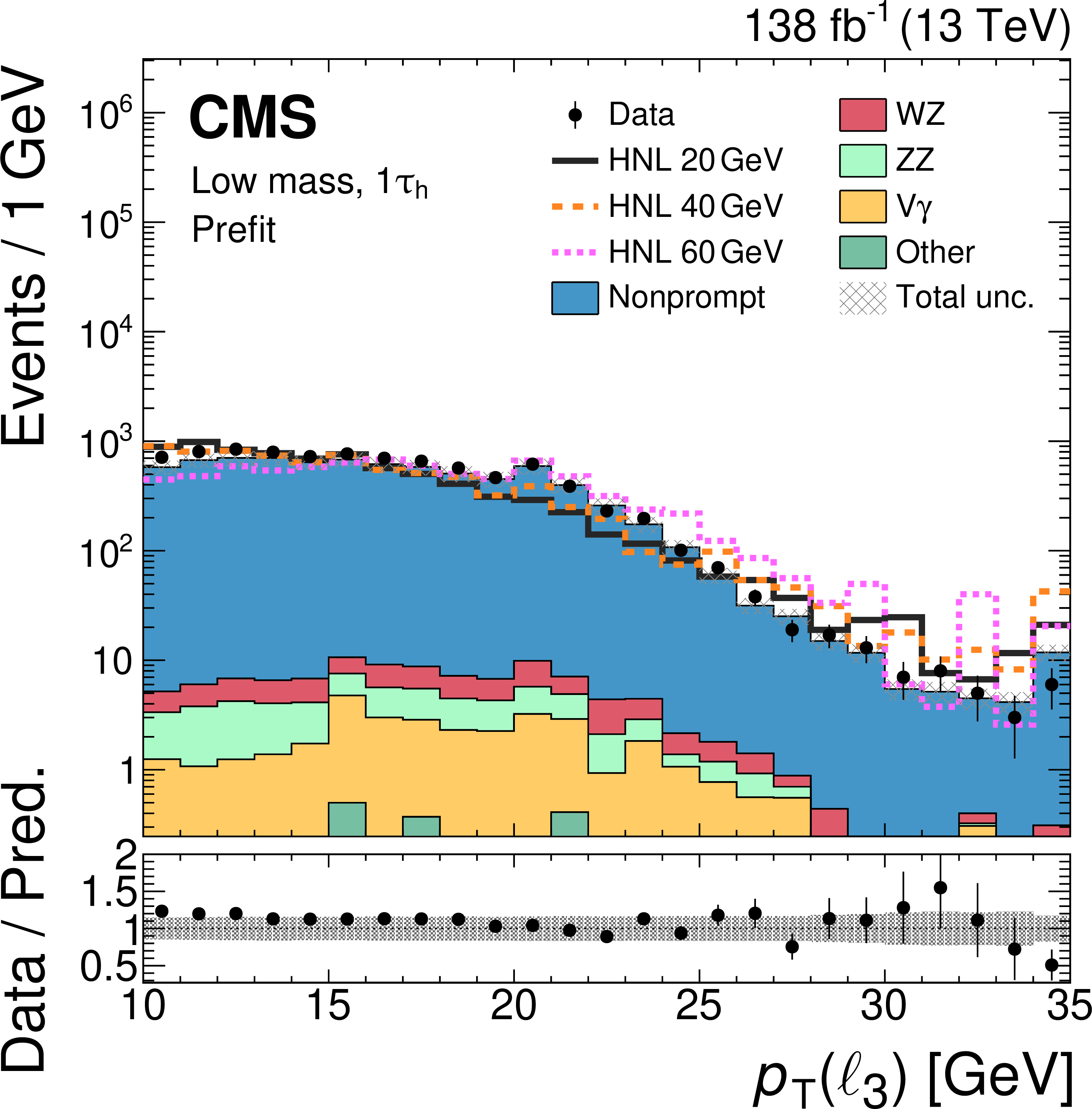
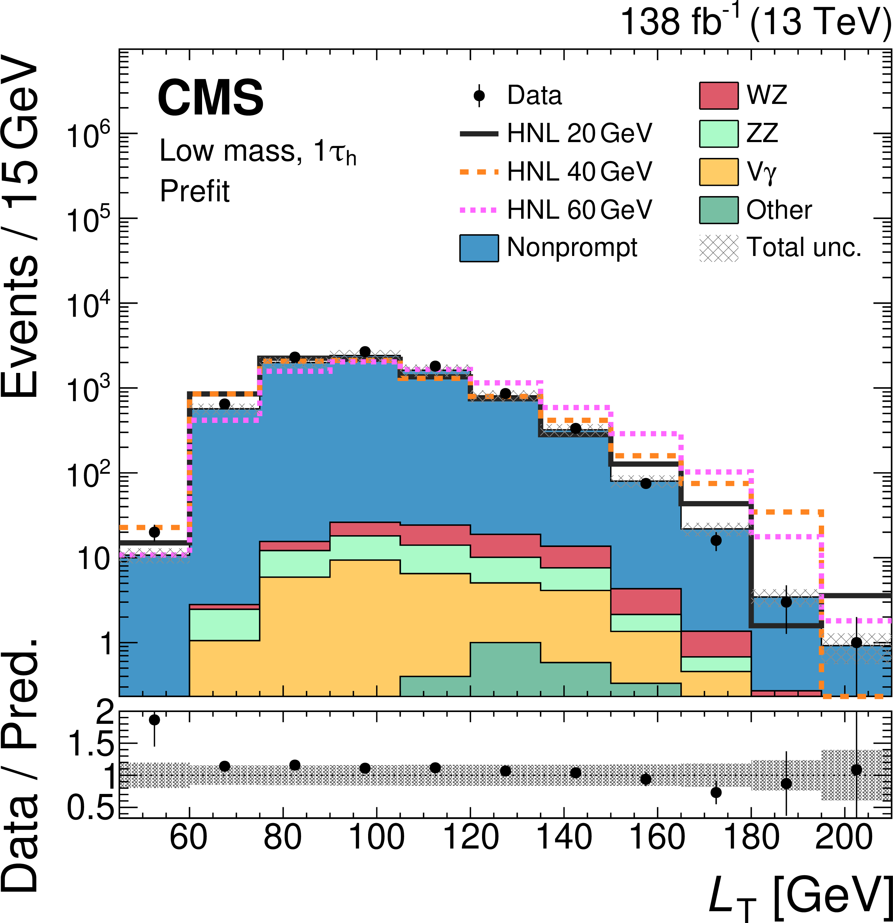
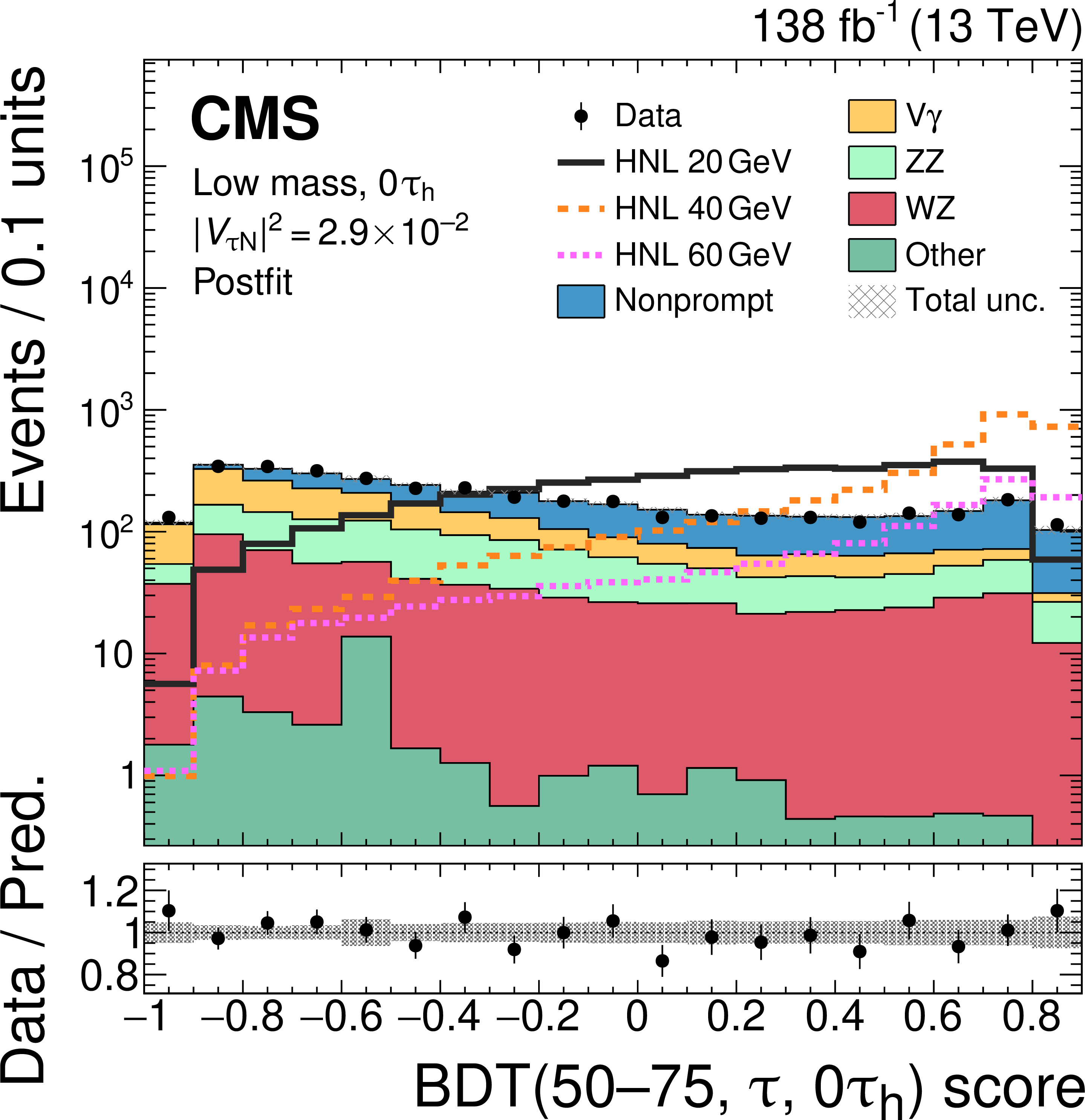
Figure 3:
Comparison of observed (points) and predicted (coloured histograms) distributions in the low-mass selection for the 1$ {\tau}{\mathrm{h}} $ categories combined. Important input variables to the BDT training are shown: $ \min m({\ell}^{+}{\ell}^{-}) $ (upper left), $p_{\mathrm{T}}(\ell_{3})$ (upper right), $ m(3$\ell$) $ (lower left), $ L_{\mathrm{T}} $ (lower right). The predicted background yields are shown before the fit to the data (``prefit''). The HNL predictions for three different $ m_{\mathrm{N}} $ values with exclusive coupling to tau neutrinos are shown with coloured lines, and are normalized to the total background yield. The vertical bars on the points represent the statistical uncertainties in the data, and the hatched bands the total uncertainties in the predictions. The last bins include the overflow contributions. In the lower panels, the ratios of the event yield in data to the overall sum of the predictions are shown. |
png pdf |
Figure 3-a:
Comparison of observed (points) and predicted (coloured histograms) distributions in the low-mass selection for the 1$ {\tau}{\mathrm{h}} $ categories combined. Important input variables to the BDT training are shown: $ \min m({\ell}^{+}{\ell}^{-}) $ (upper left), $p_{\mathrm{T}}(\ell_{3})$ (upper right), $ m(3$\ell$) $ (lower left), $ L_{\mathrm{T}} $ (lower right). The predicted background yields are shown before the fit to the data (``prefit''). The HNL predictions for three different $ m_{\mathrm{N}} $ values with exclusive coupling to tau neutrinos are shown with coloured lines, and are normalized to the total background yield. The vertical bars on the points represent the statistical uncertainties in the data, and the hatched bands the total uncertainties in the predictions. The last bins include the overflow contributions. In the lower panels, the ratios of the event yield in data to the overall sum of the predictions are shown. |
png pdf |
Figure 3-b:
Comparison of observed (points) and predicted (coloured histograms) distributions in the low-mass selection for the 1$ {\tau}{\mathrm{h}} $ categories combined. Important input variables to the BDT training are shown: $ \min m({\ell}^{+}{\ell}^{-}) $ (upper left), $p_{\mathrm{T}}(\ell_{3})$ (upper right), $ m(3$\ell$) $ (lower left), $ L_{\mathrm{T}} $ (lower right). The predicted background yields are shown before the fit to the data (``prefit''). The HNL predictions for three different $ m_{\mathrm{N}} $ values with exclusive coupling to tau neutrinos are shown with coloured lines, and are normalized to the total background yield. The vertical bars on the points represent the statistical uncertainties in the data, and the hatched bands the total uncertainties in the predictions. The last bins include the overflow contributions. In the lower panels, the ratios of the event yield in data to the overall sum of the predictions are shown. |

png pdf |
Figure 3-c:
Comparison of observed (points) and predicted (coloured histograms) distributions in the low-mass selection for the 1$ {\tau}{\mathrm{h}} $ categories combined. Important input variables to the BDT training are shown: $ \min m({\ell}^{+}{\ell}^{-}) $ (upper left), $p_{\mathrm{T}}(\ell_{3})$ (upper right), $ m(3$\ell$) $ (lower left), $ L_{\mathrm{T}} $ (lower right). The predicted background yields are shown before the fit to the data (``prefit''). The HNL predictions for three different $ m_{\mathrm{N}} $ values with exclusive coupling to tau neutrinos are shown with coloured lines, and are normalized to the total background yield. The vertical bars on the points represent the statistical uncertainties in the data, and the hatched bands the total uncertainties in the predictions. The last bins include the overflow contributions. In the lower panels, the ratios of the event yield in data to the overall sum of the predictions are shown. |
png pdf |
Figure 3-d:
Comparison of observed (points) and predicted (coloured histograms) distributions in the low-mass selection for the 1$ {\tau}{\mathrm{h}} $ categories combined. Important input variables to the BDT training are shown: $ \min m({\ell}^{+}{\ell}^{-}) $ (upper left), $p_{\mathrm{T}}(\ell_{3})$ (upper right), $ m(3$\ell$) $ (lower left), $ L_{\mathrm{T}} $ (lower right). The predicted background yields are shown before the fit to the data (``prefit''). The HNL predictions for three different $ m_{\mathrm{N}} $ values with exclusive coupling to tau neutrinos are shown with coloured lines, and are normalized to the total background yield. The vertical bars on the points represent the statistical uncertainties in the data, and the hatched bands the total uncertainties in the predictions. The last bins include the overflow contributions. In the lower panels, the ratios of the event yield in data to the overall sum of the predictions are shown. |
png pdf |
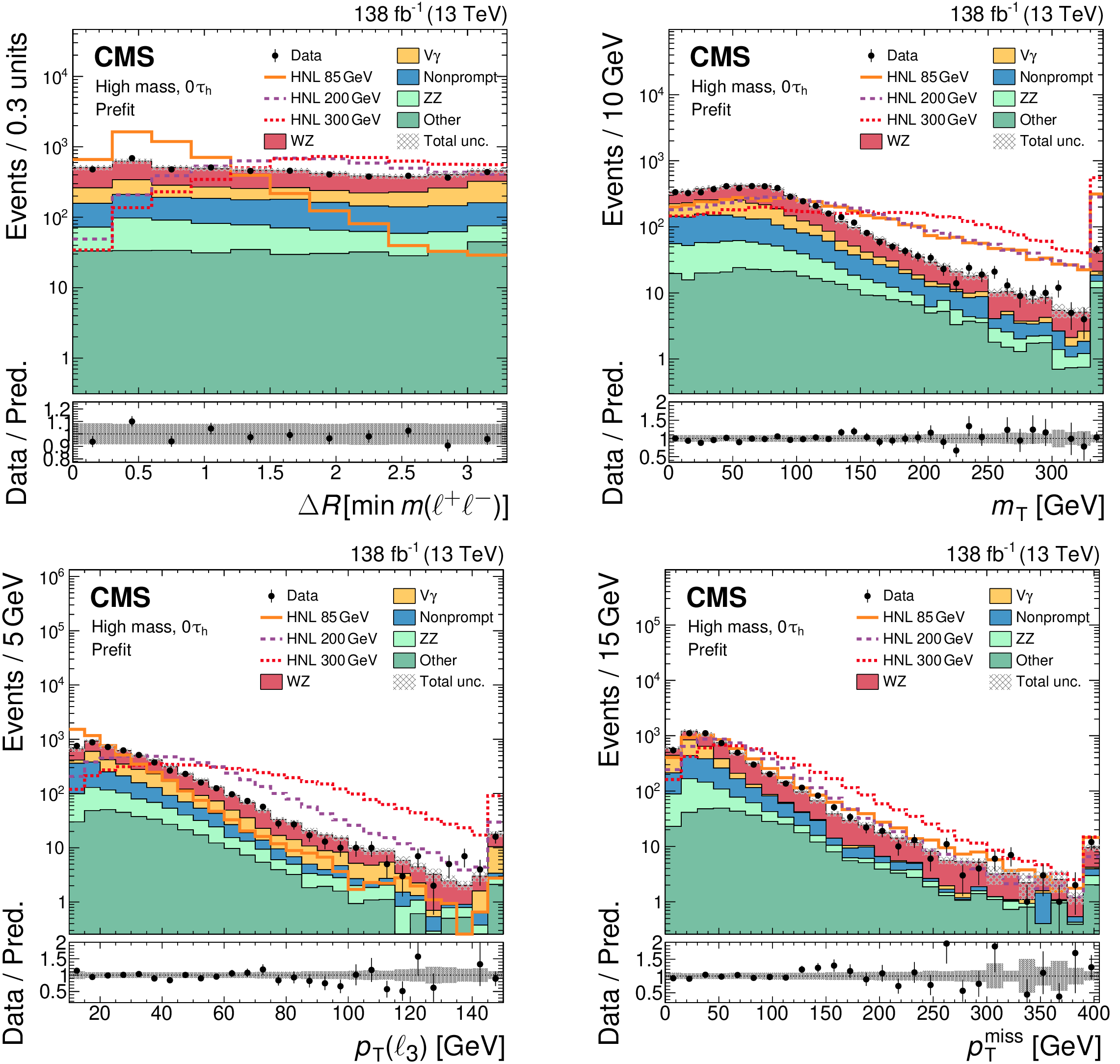
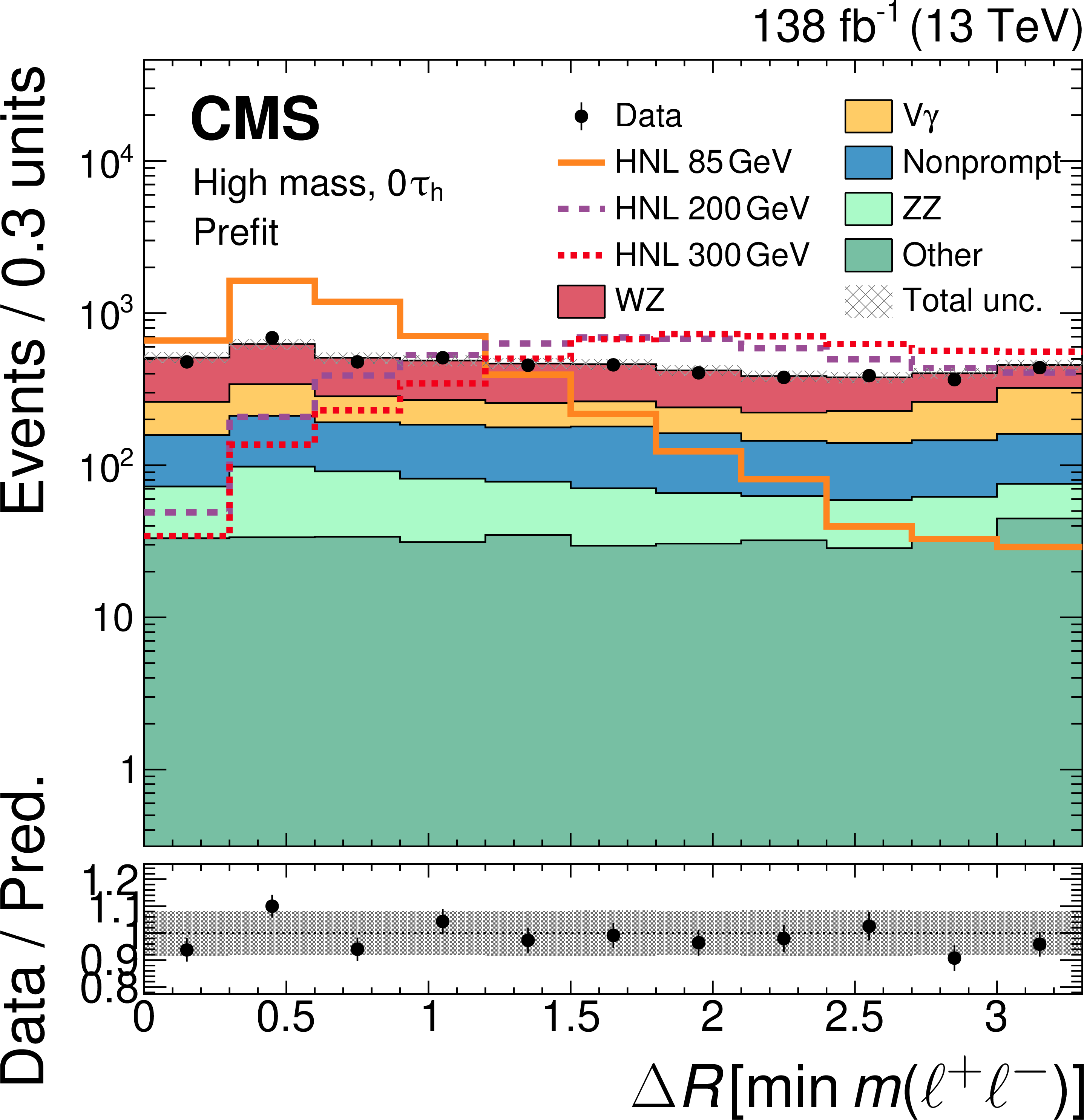
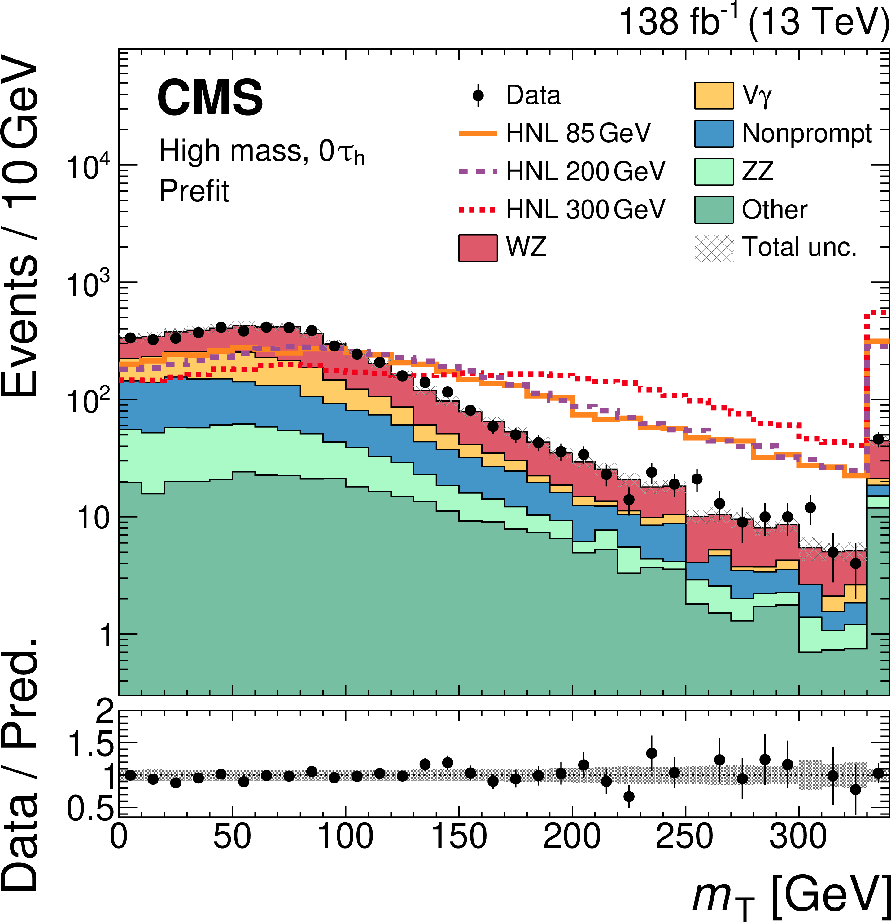
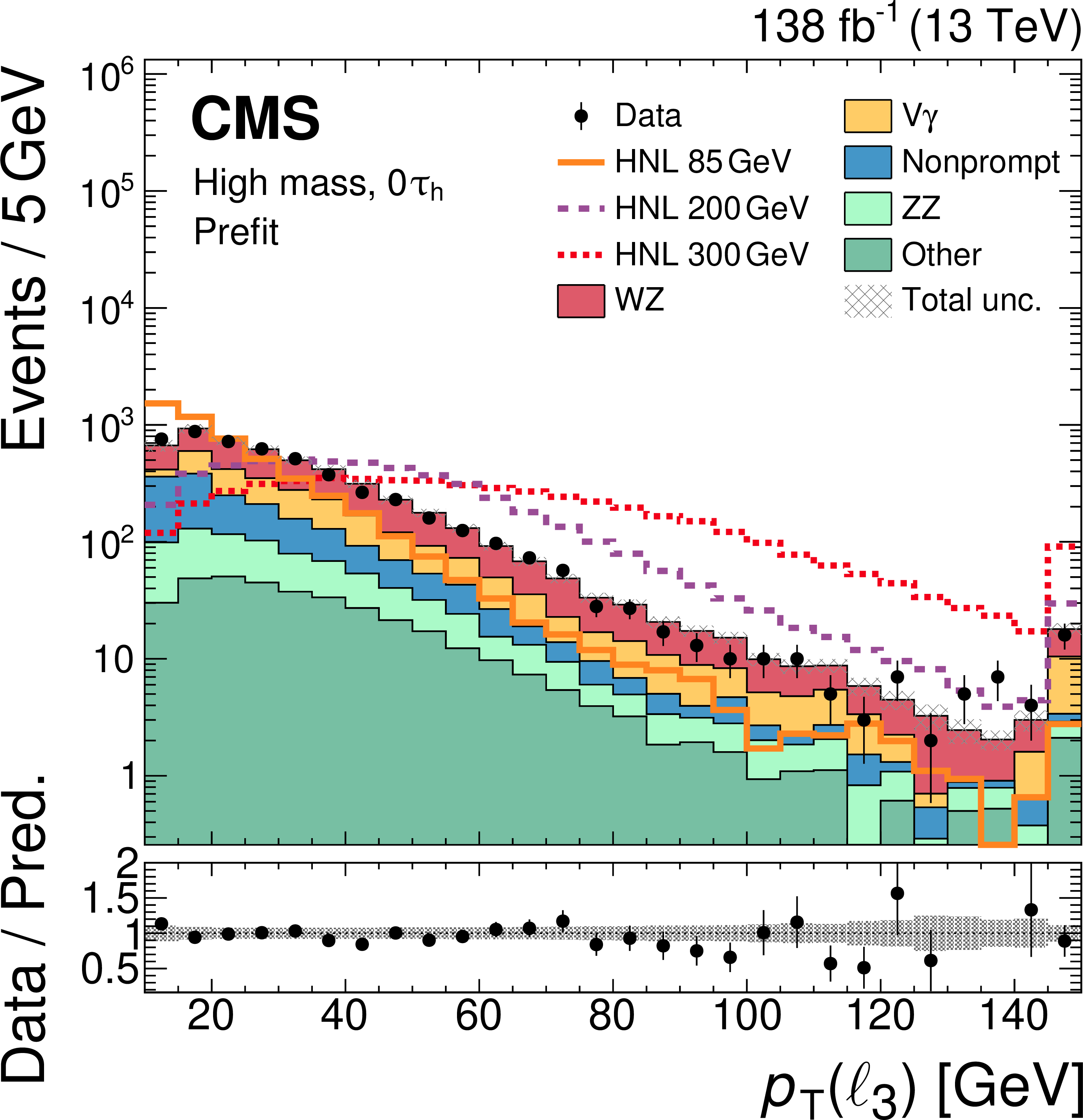
Figure 4:
Comparison of observed (points) and predicted (coloured histograms) distributions in the high-mass selection for the 0$ {\tau}{\mathrm{h}} $ categories combined. Important input variables to the BDT training are shown: $ \Delta R[\min m({\ell}^{+}{\ell}^{-})] $ (upper left), $ m_{\mathrm{T}} $ (upper right), $p_{\mathrm{T}}(\ell_{3})$ (lower left), $ p_{\mathrm{T}}^\text{miss} $ (lower right). The predicted background yields are shown before the fit to the data (``prefit''). The HNL predictions for three different $ m_{\mathrm{N}} $ values with exclusive coupling to tau neutrinos are shown with coloured lines, and are normalized to the total background yield. The vertical bars on the points represent the statistical uncertainties in the data, and the hatched bands the total uncertainties in the predictions. The last bins include the overflow contributions. In the lower panels, the ratios of the event yield in data to the overall sum of the predictions are shown. |
png pdf |
Figure 4-a:
Comparison of observed (points) and predicted (coloured histograms) distributions in the high-mass selection for the 0$ {\tau}{\mathrm{h}} $ categories combined. Important input variables to the BDT training are shown: $ \Delta R[\min m({\ell}^{+}{\ell}^{-})] $ (upper left), $ m_{\mathrm{T}} $ (upper right), $p_{\mathrm{T}}(\ell_{3})$ (lower left), $ p_{\mathrm{T}}^\text{miss} $ (lower right). The predicted background yields are shown before the fit to the data (``prefit''). The HNL predictions for three different $ m_{\mathrm{N}} $ values with exclusive coupling to tau neutrinos are shown with coloured lines, and are normalized to the total background yield. The vertical bars on the points represent the statistical uncertainties in the data, and the hatched bands the total uncertainties in the predictions. The last bins include the overflow contributions. In the lower panels, the ratios of the event yield in data to the overall sum of the predictions are shown. |
png pdf |
Figure 4-b:
Comparison of observed (points) and predicted (coloured histograms) distributions in the high-mass selection for the 0$ {\tau}{\mathrm{h}} $ categories combined. Important input variables to the BDT training are shown: $ \Delta R[\min m({\ell}^{+}{\ell}^{-})] $ (upper left), $ m_{\mathrm{T}} $ (upper right), $p_{\mathrm{T}}(\ell_{3})$ (lower left), $ p_{\mathrm{T}}^\text{miss} $ (lower right). The predicted background yields are shown before the fit to the data (``prefit''). The HNL predictions for three different $ m_{\mathrm{N}} $ values with exclusive coupling to tau neutrinos are shown with coloured lines, and are normalized to the total background yield. The vertical bars on the points represent the statistical uncertainties in the data, and the hatched bands the total uncertainties in the predictions. The last bins include the overflow contributions. In the lower panels, the ratios of the event yield in data to the overall sum of the predictions are shown. |
png pdf |
Figure 4-c:
Comparison of observed (points) and predicted (coloured histograms) distributions in the high-mass selection for the 0$ {\tau}{\mathrm{h}} $ categories combined. Important input variables to the BDT training are shown: $ \Delta R[\min m({\ell}^{+}{\ell}^{-})] $ (upper left), $ m_{\mathrm{T}} $ (upper right), $p_{\mathrm{T}}(\ell_{3})$ (lower left), $ p_{\mathrm{T}}^\text{miss} $ (lower right). The predicted background yields are shown before the fit to the data (``prefit''). The HNL predictions for three different $ m_{\mathrm{N}} $ values with exclusive coupling to tau neutrinos are shown with coloured lines, and are normalized to the total background yield. The vertical bars on the points represent the statistical uncertainties in the data, and the hatched bands the total uncertainties in the predictions. The last bins include the overflow contributions. In the lower panels, the ratios of the event yield in data to the overall sum of the predictions are shown. |

png pdf |
Figure 4-d:
Comparison of observed (points) and predicted (coloured histograms) distributions in the high-mass selection for the 0$ {\tau}{\mathrm{h}} $ categories combined. Important input variables to the BDT training are shown: $ \Delta R[\min m({\ell}^{+}{\ell}^{-})] $ (upper left), $ m_{\mathrm{T}} $ (upper right), $p_{\mathrm{T}}(\ell_{3})$ (lower left), $ p_{\mathrm{T}}^\text{miss} $ (lower right). The predicted background yields are shown before the fit to the data (``prefit''). The HNL predictions for three different $ m_{\mathrm{N}} $ values with exclusive coupling to tau neutrinos are shown with coloured lines, and are normalized to the total background yield. The vertical bars on the points represent the statistical uncertainties in the data, and the hatched bands the total uncertainties in the predictions. The last bins include the overflow contributions. In the lower panels, the ratios of the event yield in data to the overall sum of the predictions are shown. |
png pdf |
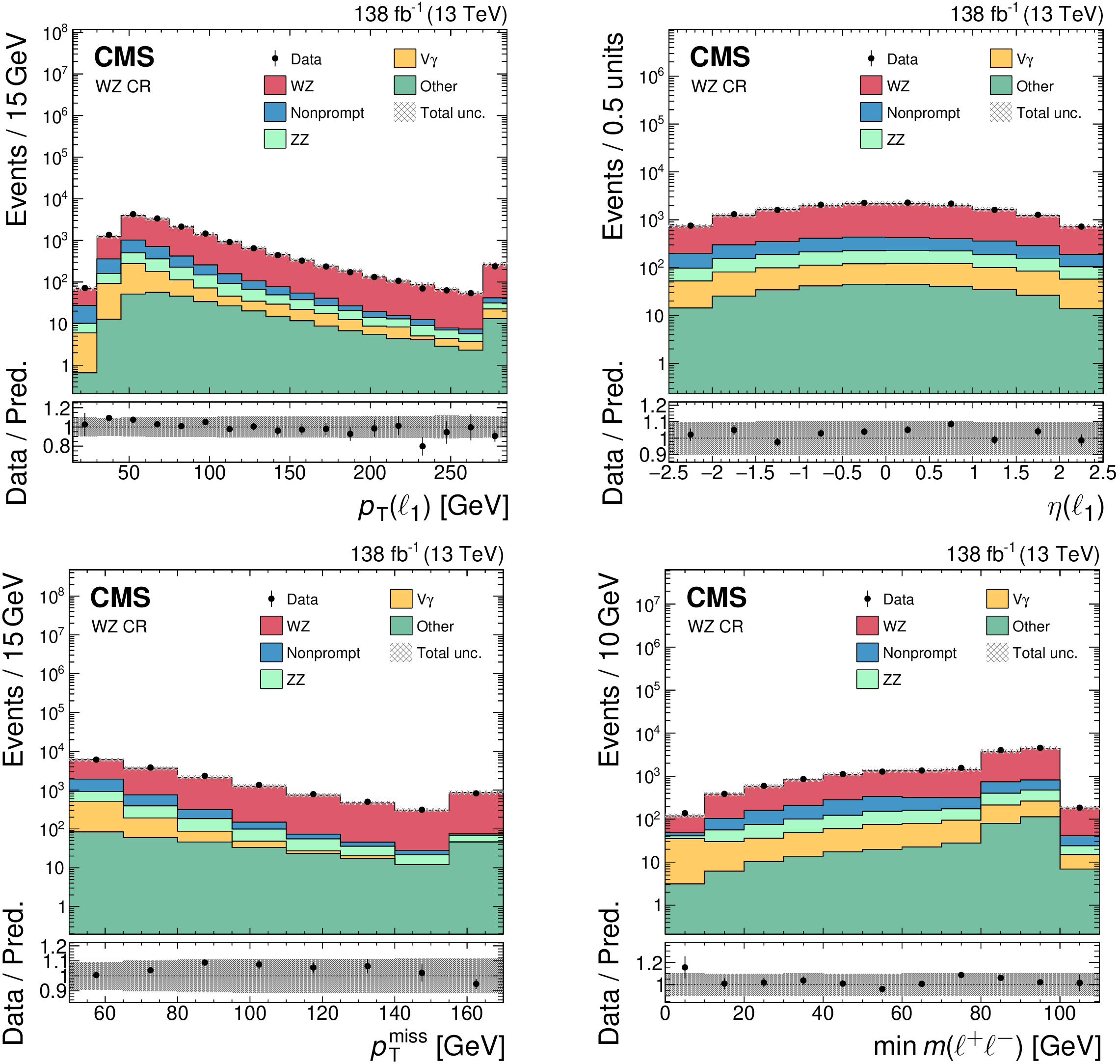
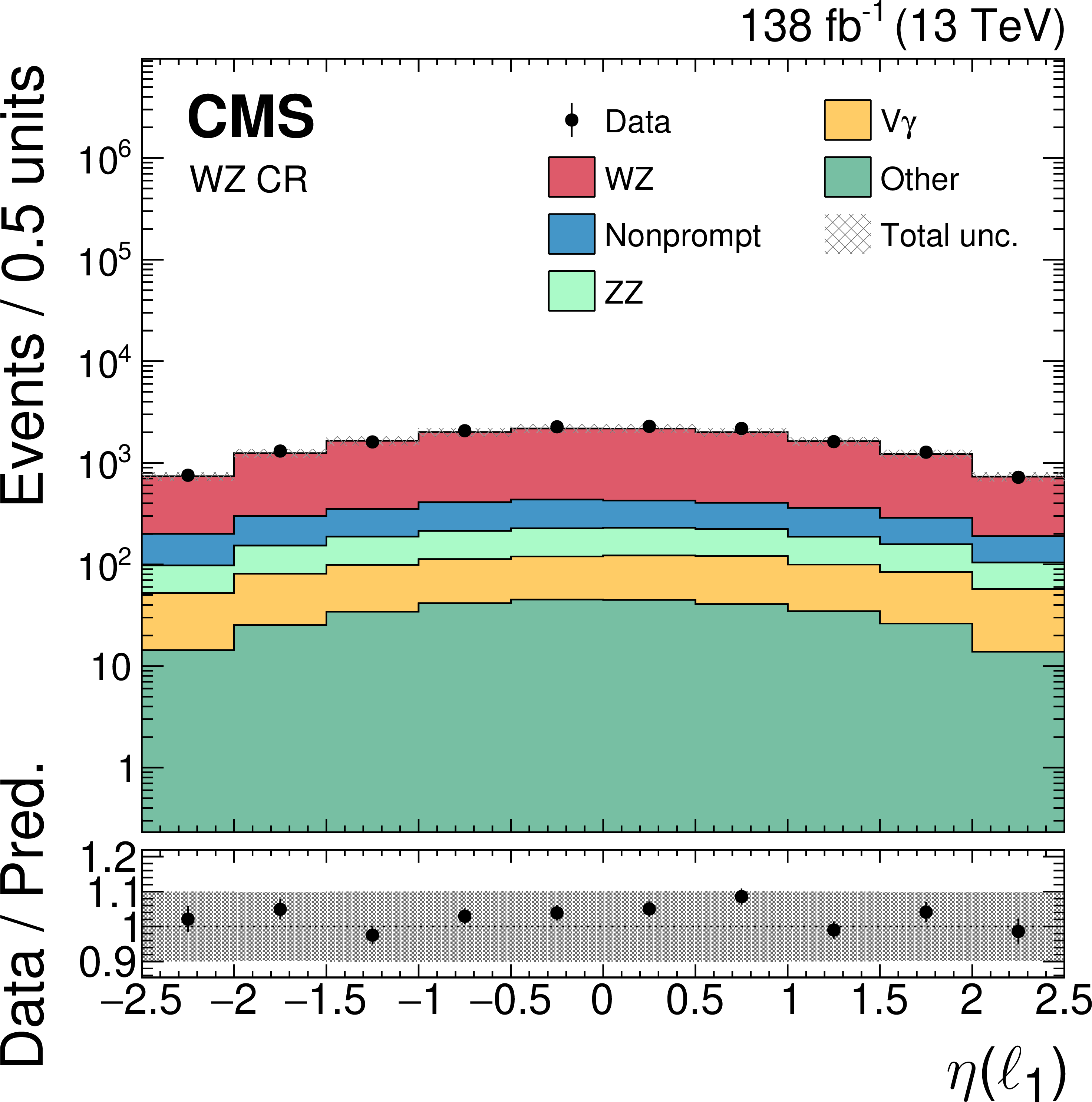
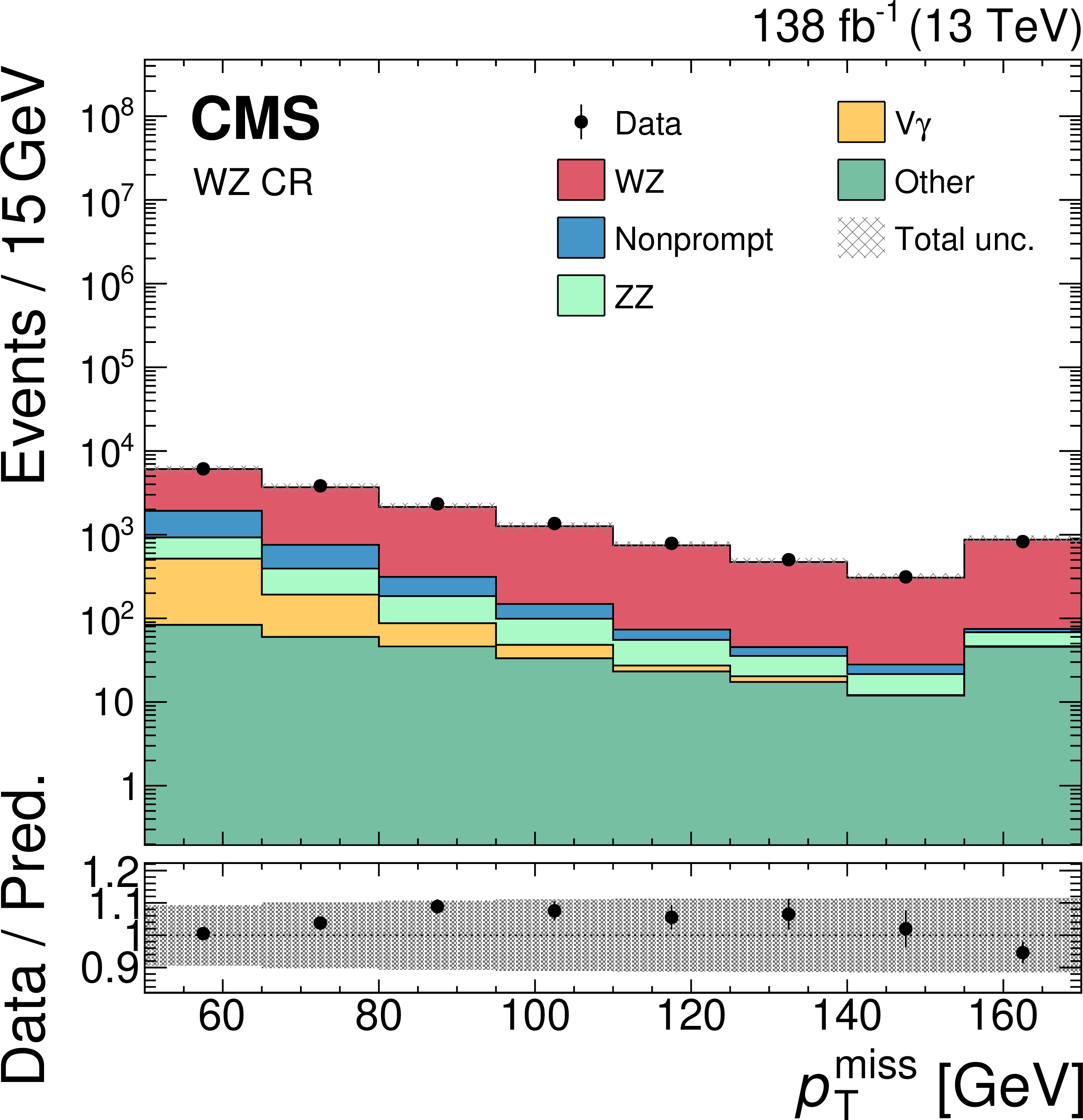
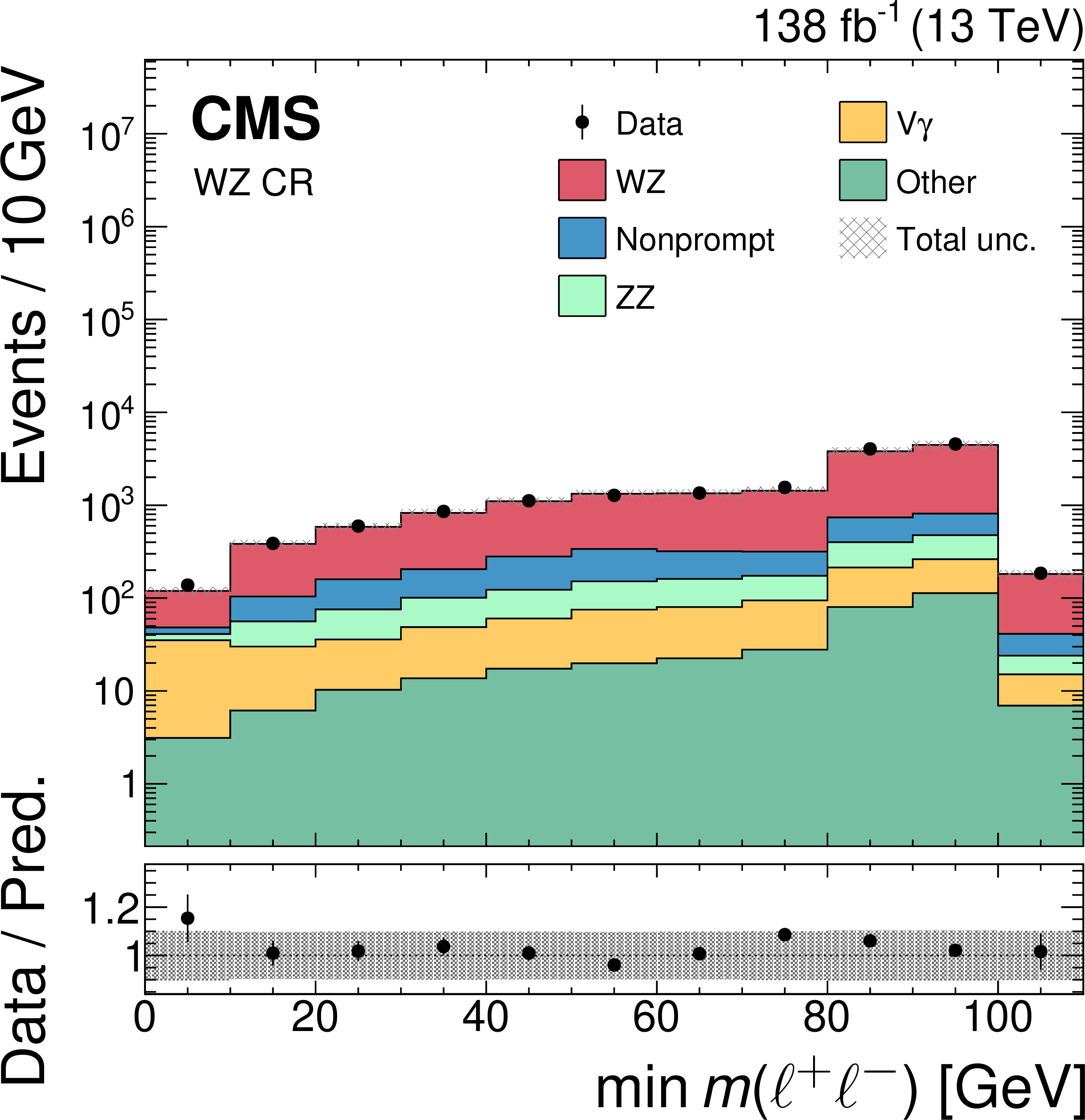
Figure 5:
Comparison of observed (points) and predicted (coloured histograms) distributions in the WZ CR. The leading lepton $ p_{\mathrm{T}} $ (upper left) and $ \eta $ (upper right), as well as $ p_{\mathrm{T}}^\text{miss} $ (lower left) and $ \min m({\ell}^{+}{\ell}^{-}) $ (lower right) are shown. The vertical bars on the points represent the statistical uncertainties in the data, and the hatched bands the total uncertainties in the predictions. The last bins include the overflow contributions. In the lower panels, the ratios of the event yield in data to the overall sum of the predictions are shown. |

png pdf |
Figure 5-a:
Comparison of observed (points) and predicted (coloured histograms) distributions in the WZ CR. The leading lepton $ p_{\mathrm{T}} $ (upper left) and $ \eta $ (upper right), as well as $ p_{\mathrm{T}}^\text{miss} $ (lower left) and $ \min m({\ell}^{+}{\ell}^{-}) $ (lower right) are shown. The vertical bars on the points represent the statistical uncertainties in the data, and the hatched bands the total uncertainties in the predictions. The last bins include the overflow contributions. In the lower panels, the ratios of the event yield in data to the overall sum of the predictions are shown. |
png pdf |
Figure 5-b:
Comparison of observed (points) and predicted (coloured histograms) distributions in the WZ CR. The leading lepton $ p_{\mathrm{T}} $ (upper left) and $ \eta $ (upper right), as well as $ p_{\mathrm{T}}^\text{miss} $ (lower left) and $ \min m({\ell}^{+}{\ell}^{-}) $ (lower right) are shown. The vertical bars on the points represent the statistical uncertainties in the data, and the hatched bands the total uncertainties in the predictions. The last bins include the overflow contributions. In the lower panels, the ratios of the event yield in data to the overall sum of the predictions are shown. |
png pdf |
Figure 5-c:
Comparison of observed (points) and predicted (coloured histograms) distributions in the WZ CR. The leading lepton $ p_{\mathrm{T}} $ (upper left) and $ \eta $ (upper right), as well as $ p_{\mathrm{T}}^\text{miss} $ (lower left) and $ \min m({\ell}^{+}{\ell}^{-}) $ (lower right) are shown. The vertical bars on the points represent the statistical uncertainties in the data, and the hatched bands the total uncertainties in the predictions. The last bins include the overflow contributions. In the lower panels, the ratios of the event yield in data to the overall sum of the predictions are shown. |
png pdf |
Figure 5-d:
Comparison of observed (points) and predicted (coloured histograms) distributions in the WZ CR. The leading lepton $ p_{\mathrm{T}} $ (upper left) and $ \eta $ (upper right), as well as $ p_{\mathrm{T}}^\text{miss} $ (lower left) and $ \min m({\ell}^{+}{\ell}^{-}) $ (lower right) are shown. The vertical bars on the points represent the statistical uncertainties in the data, and the hatched bands the total uncertainties in the predictions. The last bins include the overflow contributions. In the lower panels, the ratios of the event yield in data to the overall sum of the predictions are shown. |
png pdf |
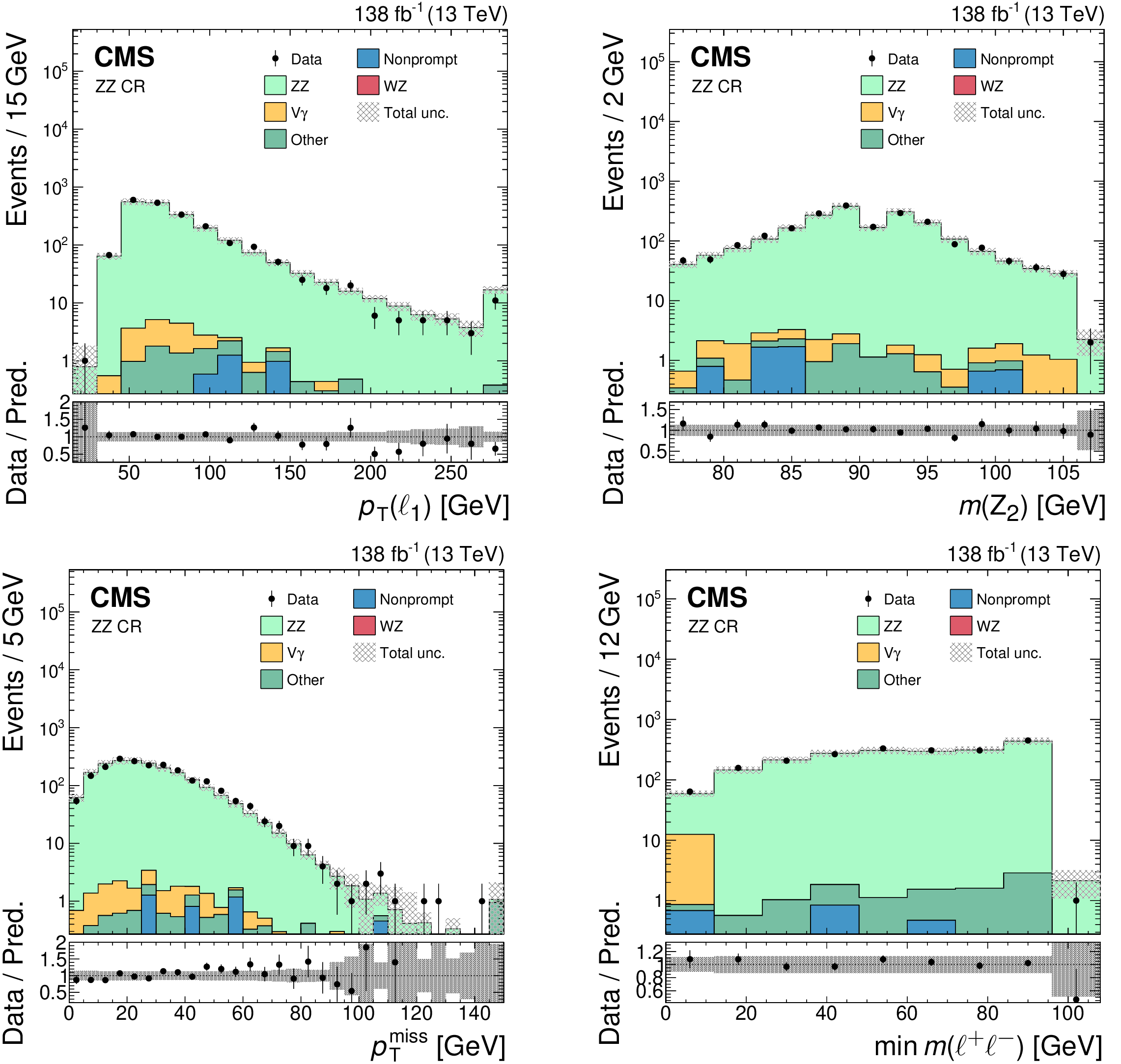
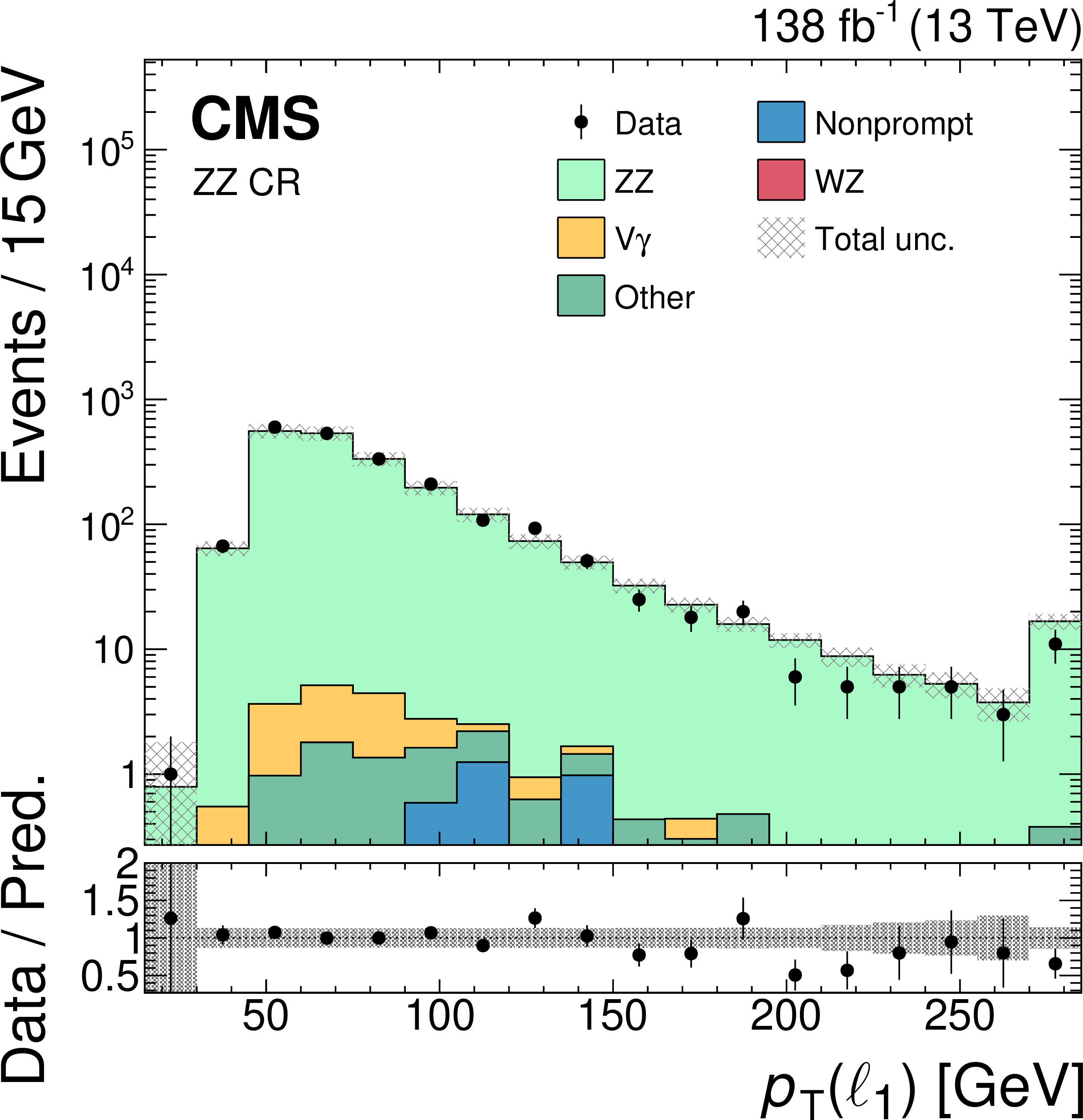
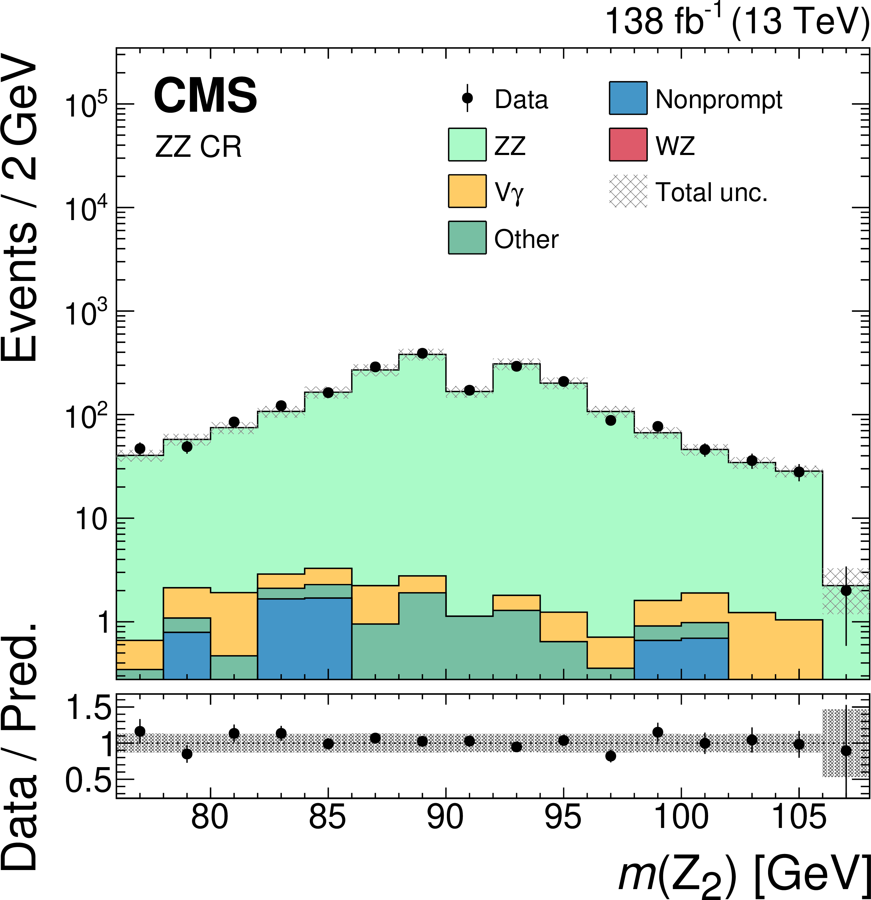
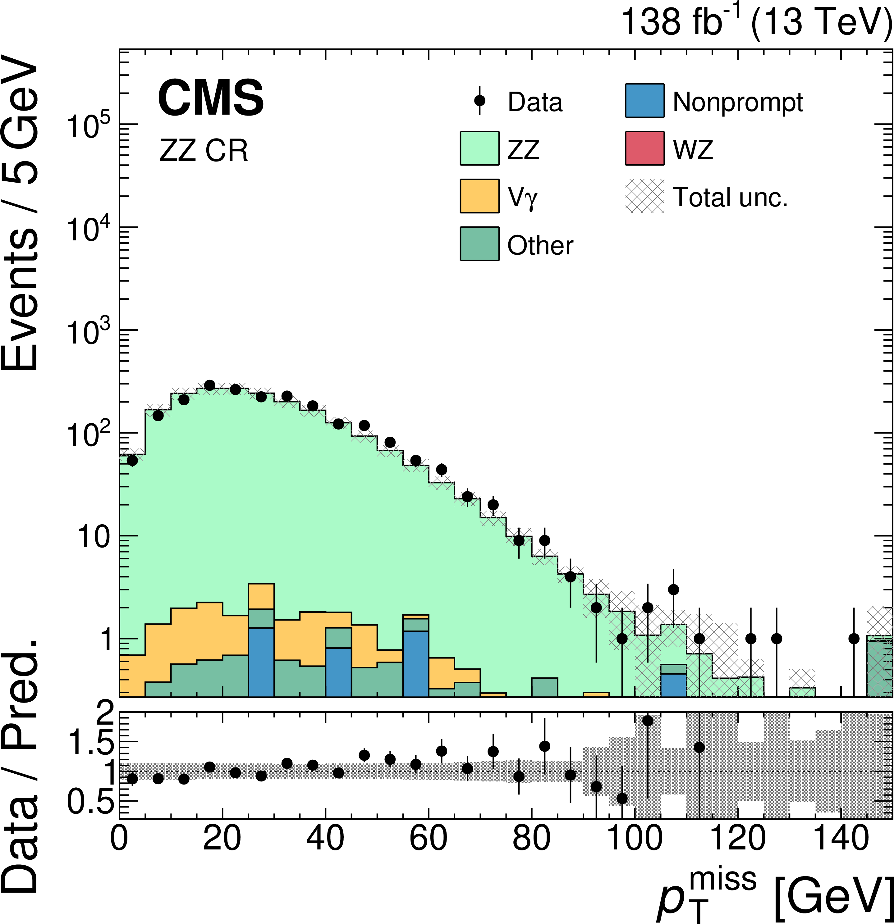
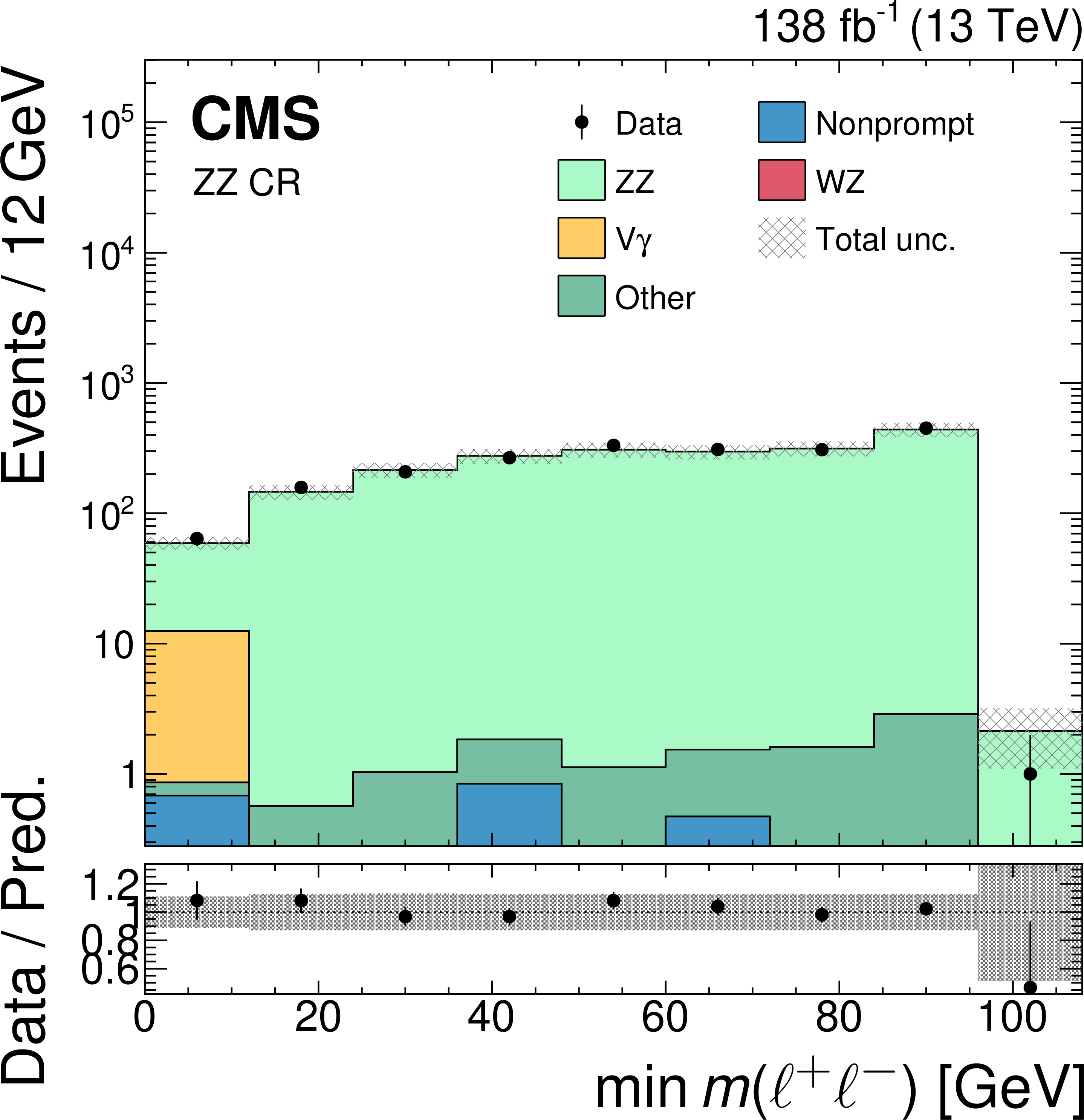
Figure 6:
Comparison of observed (points) and predicted (coloured histograms) distributions in the ZZ CR. The leading lepton $ p_{\mathrm{T}} $ (upper left), $ m({\ell}^{+}{\ell}^{-}) $ of $ \mathrm{Z}_2 $ ($ m(\mathrm{Z}_2) $, upper right), $ p_{\mathrm{T}}^\text{miss} $ (lower left), and $ \min m({\ell}^{+}{\ell}^{-}) $ (lower right) are shown. The ZZ prediction is scaled with a normalization factor of 1.12, as discussed in the text. The vertical bars on the points represent the statistical uncertainties in the data, and the hatched bands the total uncertainties in the predictions. The last bins include the overflow contributions. In the lower panels, the ratios of the event yield in data to the overall sum of the predictions are shown. |
png pdf |
Figure 6-a:
Comparison of observed (points) and predicted (coloured histograms) distributions in the ZZ CR. The leading lepton $ p_{\mathrm{T}} $ (upper left), $ m({\ell}^{+}{\ell}^{-}) $ of $ \mathrm{Z}_2 $ ($ m(\mathrm{Z}_2) $, upper right), $ p_{\mathrm{T}}^\text{miss} $ (lower left), and $ \min m({\ell}^{+}{\ell}^{-}) $ (lower right) are shown. The ZZ prediction is scaled with a normalization factor of 1.12, as discussed in the text. The vertical bars on the points represent the statistical uncertainties in the data, and the hatched bands the total uncertainties in the predictions. The last bins include the overflow contributions. In the lower panels, the ratios of the event yield in data to the overall sum of the predictions are shown. |
png pdf |
Figure 6-b:
Comparison of observed (points) and predicted (coloured histograms) distributions in the ZZ CR. The leading lepton $ p_{\mathrm{T}} $ (upper left), $ m({\ell}^{+}{\ell}^{-}) $ of $ \mathrm{Z}_2 $ ($ m(\mathrm{Z}_2) $, upper right), $ p_{\mathrm{T}}^\text{miss} $ (lower left), and $ \min m({\ell}^{+}{\ell}^{-}) $ (lower right) are shown. The ZZ prediction is scaled with a normalization factor of 1.12, as discussed in the text. The vertical bars on the points represent the statistical uncertainties in the data, and the hatched bands the total uncertainties in the predictions. The last bins include the overflow contributions. In the lower panels, the ratios of the event yield in data to the overall sum of the predictions are shown. |
png pdf |
Figure 6-c:
Comparison of observed (points) and predicted (coloured histograms) distributions in the ZZ CR. The leading lepton $ p_{\mathrm{T}} $ (upper left), $ m({\ell}^{+}{\ell}^{-}) $ of $ \mathrm{Z}_2 $ ($ m(\mathrm{Z}_2) $, upper right), $ p_{\mathrm{T}}^\text{miss} $ (lower left), and $ \min m({\ell}^{+}{\ell}^{-}) $ (lower right) are shown. The ZZ prediction is scaled with a normalization factor of 1.12, as discussed in the text. The vertical bars on the points represent the statistical uncertainties in the data, and the hatched bands the total uncertainties in the predictions. The last bins include the overflow contributions. In the lower panels, the ratios of the event yield in data to the overall sum of the predictions are shown. |
png pdf |
Figure 6-d:
Comparison of observed (points) and predicted (coloured histograms) distributions in the ZZ CR. The leading lepton $ p_{\mathrm{T}} $ (upper left), $ m({\ell}^{+}{\ell}^{-}) $ of $ \mathrm{Z}_2 $ ($ m(\mathrm{Z}_2) $, upper right), $ p_{\mathrm{T}}^\text{miss} $ (lower left), and $ \min m({\ell}^{+}{\ell}^{-}) $ (lower right) are shown. The ZZ prediction is scaled with a normalization factor of 1.12, as discussed in the text. The vertical bars on the points represent the statistical uncertainties in the data, and the hatched bands the total uncertainties in the predictions. The last bins include the overflow contributions. In the lower panels, the ratios of the event yield in data to the overall sum of the predictions are shown. |

png pdf |
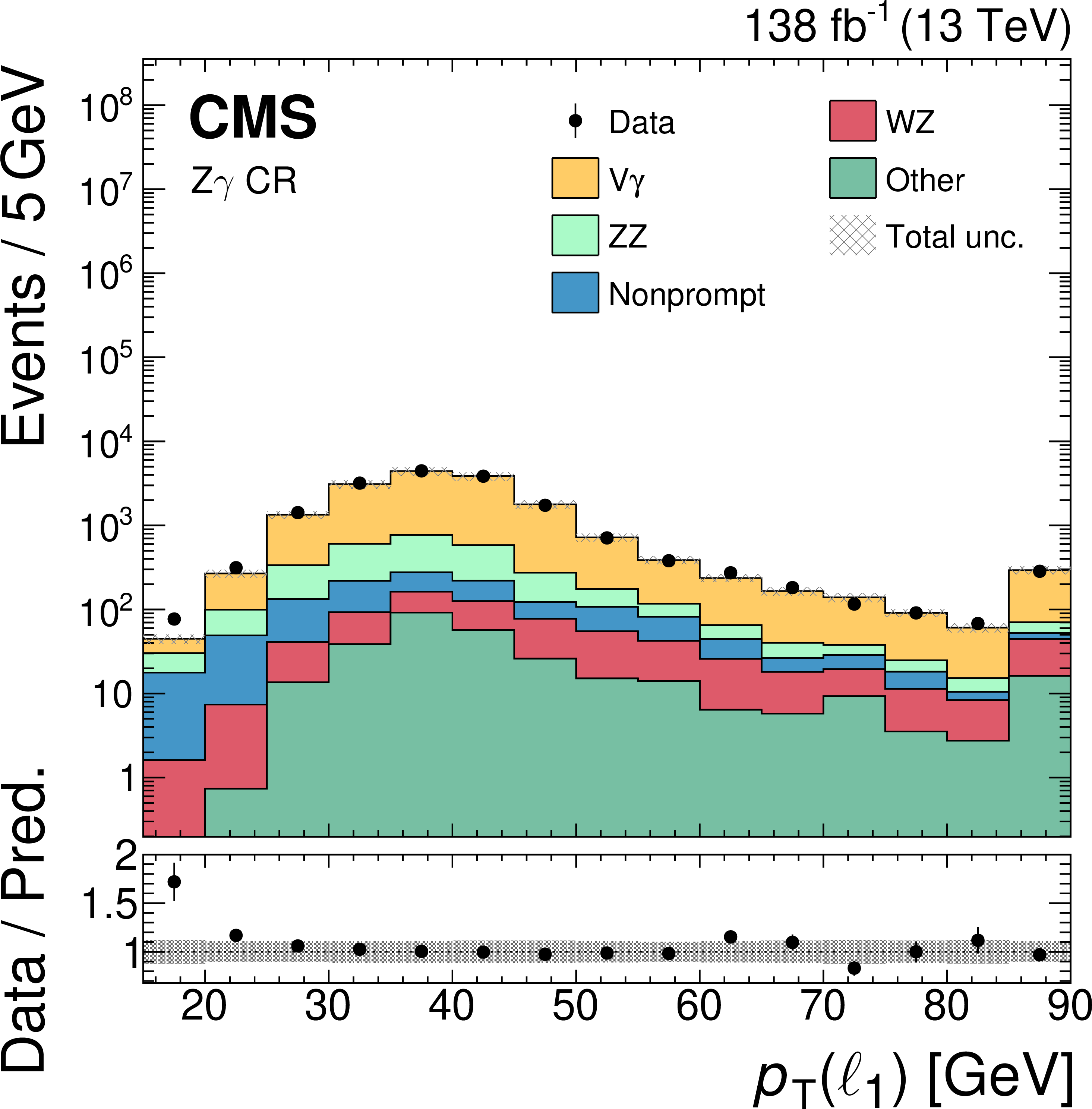
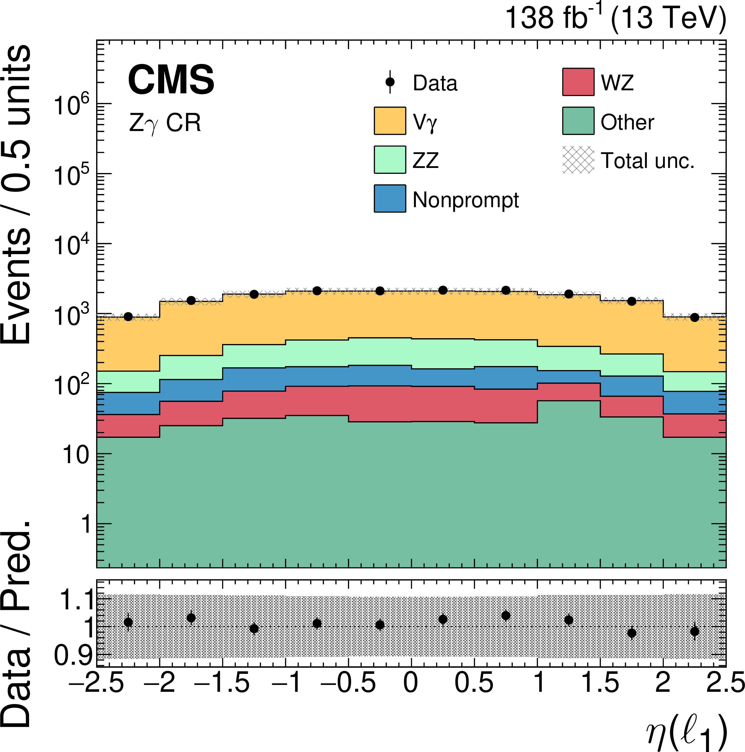
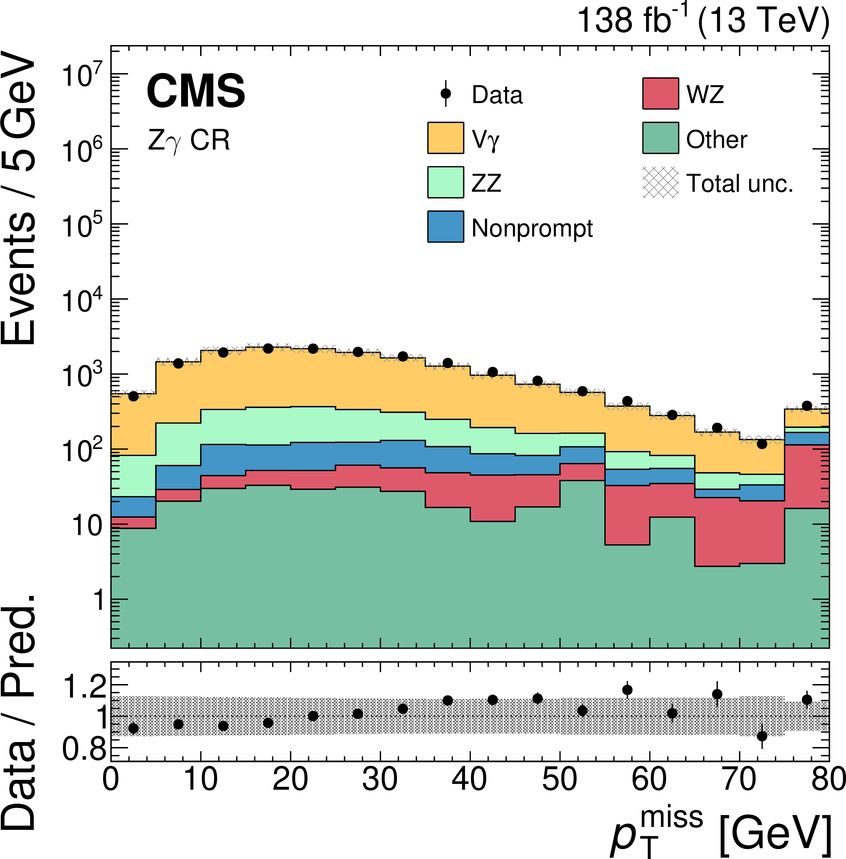
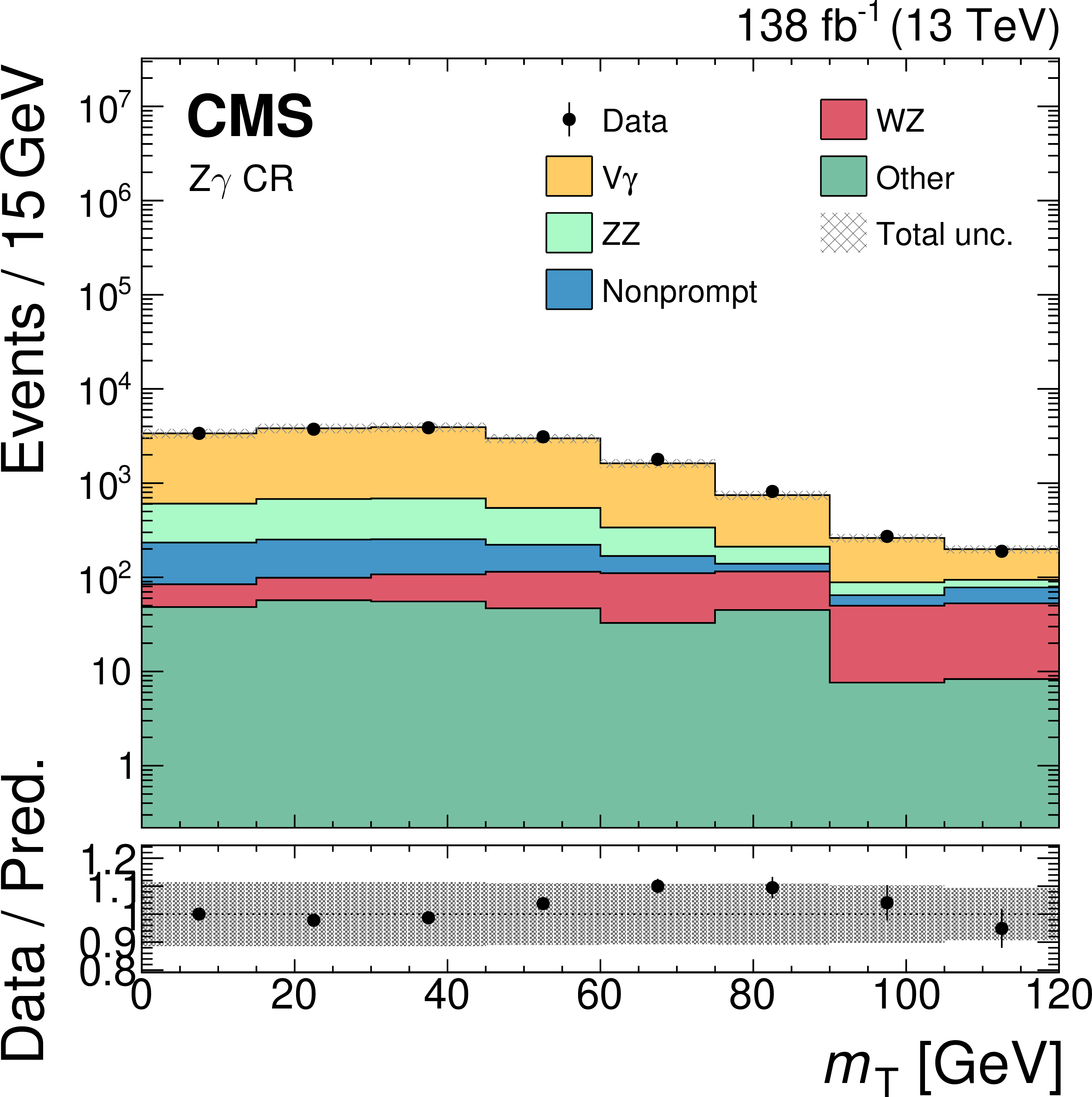
Figure 7:
Comparison of observed (points) and predicted (coloured histograms) distributions in the $ \mathrm{Z}\gamma $ CR. The leading lepton $ p_{\mathrm{T}} $ (upper left) and $ \eta $ (upper right), $ p_{\mathrm{T}}^\text{miss} $ (lower left), and $ m_{\mathrm{T}} $ (lower right) are shown. The $ \mathrm{Z}\gamma $ prediction is scaled with a normalization factor of 1.11, as discussed in the text. The vertical bars on the points represent the statistical uncertainties in the data, and the hatched bands the total uncertainties in the predictions. The last bins include the overflow contributions. In the lower panels, the ratios of the event yield in data to the overall sum of the predictions are shown. |
png pdf |
Figure 7-a:
Comparison of observed (points) and predicted (coloured histograms) distributions in the $ \mathrm{Z}\gamma $ CR. The leading lepton $ p_{\mathrm{T}} $ (upper left) and $ \eta $ (upper right), $ p_{\mathrm{T}}^\text{miss} $ (lower left), and $ m_{\mathrm{T}} $ (lower right) are shown. The $ \mathrm{Z}\gamma $ prediction is scaled with a normalization factor of 1.11, as discussed in the text. The vertical bars on the points represent the statistical uncertainties in the data, and the hatched bands the total uncertainties in the predictions. The last bins include the overflow contributions. In the lower panels, the ratios of the event yield in data to the overall sum of the predictions are shown. |
png pdf |
Figure 7-b:
Comparison of observed (points) and predicted (coloured histograms) distributions in the $ \mathrm{Z}\gamma $ CR. The leading lepton $ p_{\mathrm{T}} $ (upper left) and $ \eta $ (upper right), $ p_{\mathrm{T}}^\text{miss} $ (lower left), and $ m_{\mathrm{T}} $ (lower right) are shown. The $ \mathrm{Z}\gamma $ prediction is scaled with a normalization factor of 1.11, as discussed in the text. The vertical bars on the points represent the statistical uncertainties in the data, and the hatched bands the total uncertainties in the predictions. The last bins include the overflow contributions. In the lower panels, the ratios of the event yield in data to the overall sum of the predictions are shown. |
png pdf |
Figure 7-c:
Comparison of observed (points) and predicted (coloured histograms) distributions in the $ \mathrm{Z}\gamma $ CR. The leading lepton $ p_{\mathrm{T}} $ (upper left) and $ \eta $ (upper right), $ p_{\mathrm{T}}^\text{miss} $ (lower left), and $ m_{\mathrm{T}} $ (lower right) are shown. The $ \mathrm{Z}\gamma $ prediction is scaled with a normalization factor of 1.11, as discussed in the text. The vertical bars on the points represent the statistical uncertainties in the data, and the hatched bands the total uncertainties in the predictions. The last bins include the overflow contributions. In the lower panels, the ratios of the event yield in data to the overall sum of the predictions are shown. |
png pdf |
Figure 7-d:
Comparison of observed (points) and predicted (coloured histograms) distributions in the $ \mathrm{Z}\gamma $ CR. The leading lepton $ p_{\mathrm{T}} $ (upper left) and $ \eta $ (upper right), $ p_{\mathrm{T}}^\text{miss} $ (lower left), and $ m_{\mathrm{T}} $ (lower right) are shown. The $ \mathrm{Z}\gamma $ prediction is scaled with a normalization factor of 1.11, as discussed in the text. The vertical bars on the points represent the statistical uncertainties in the data, and the hatched bands the total uncertainties in the predictions. The last bins include the overflow contributions. In the lower panels, the ratios of the event yield in data to the overall sum of the predictions are shown. |
png pdf |
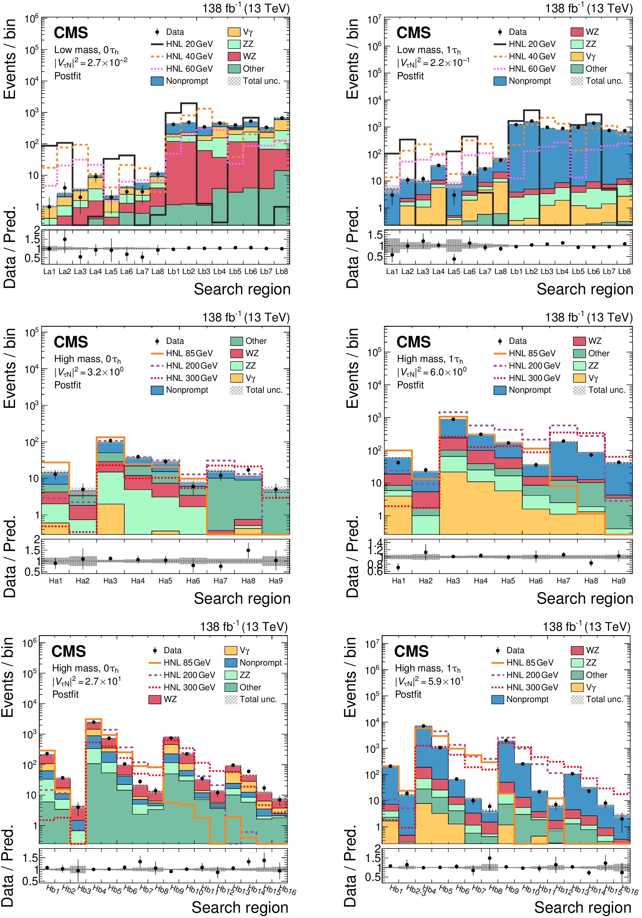
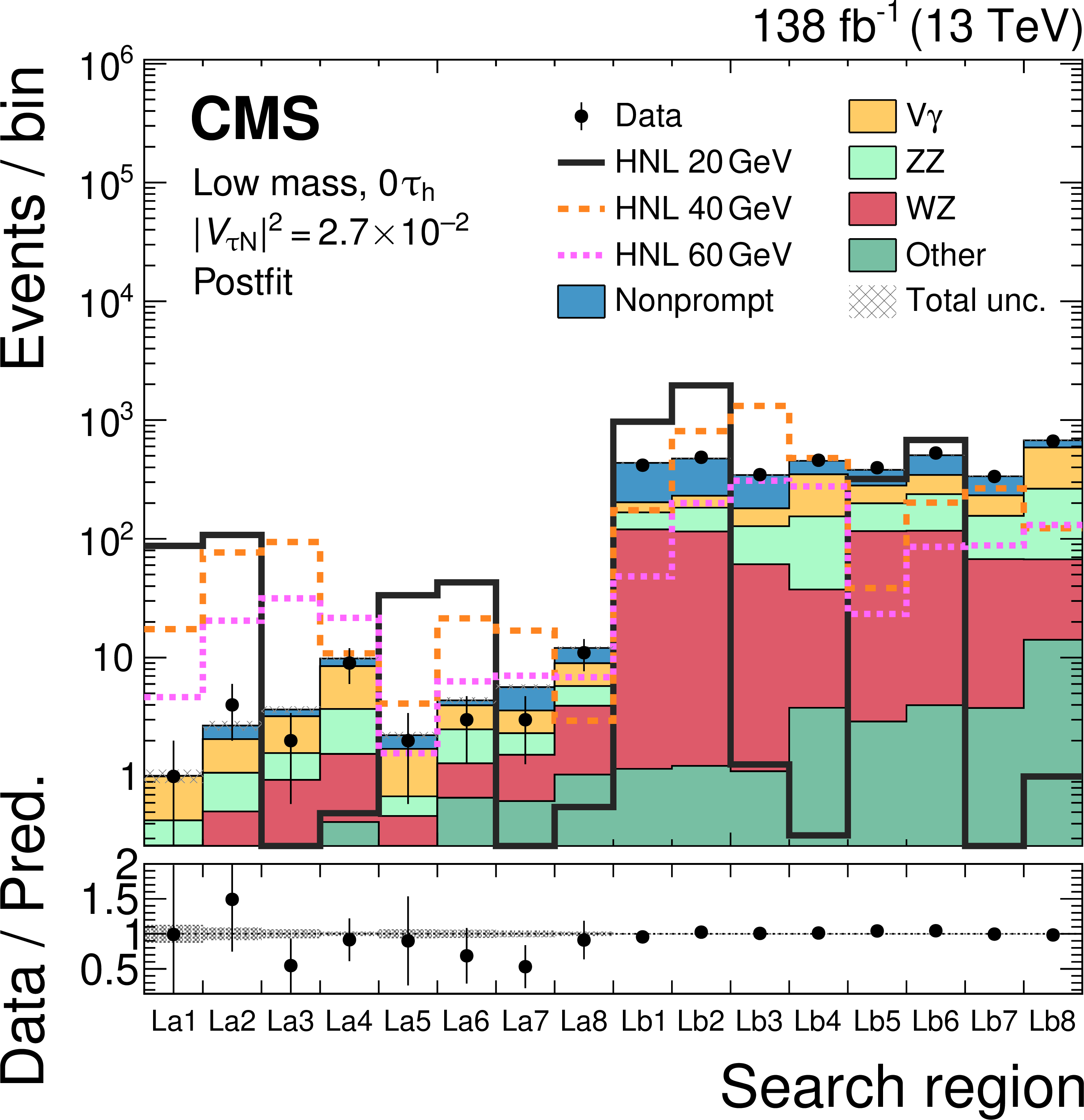
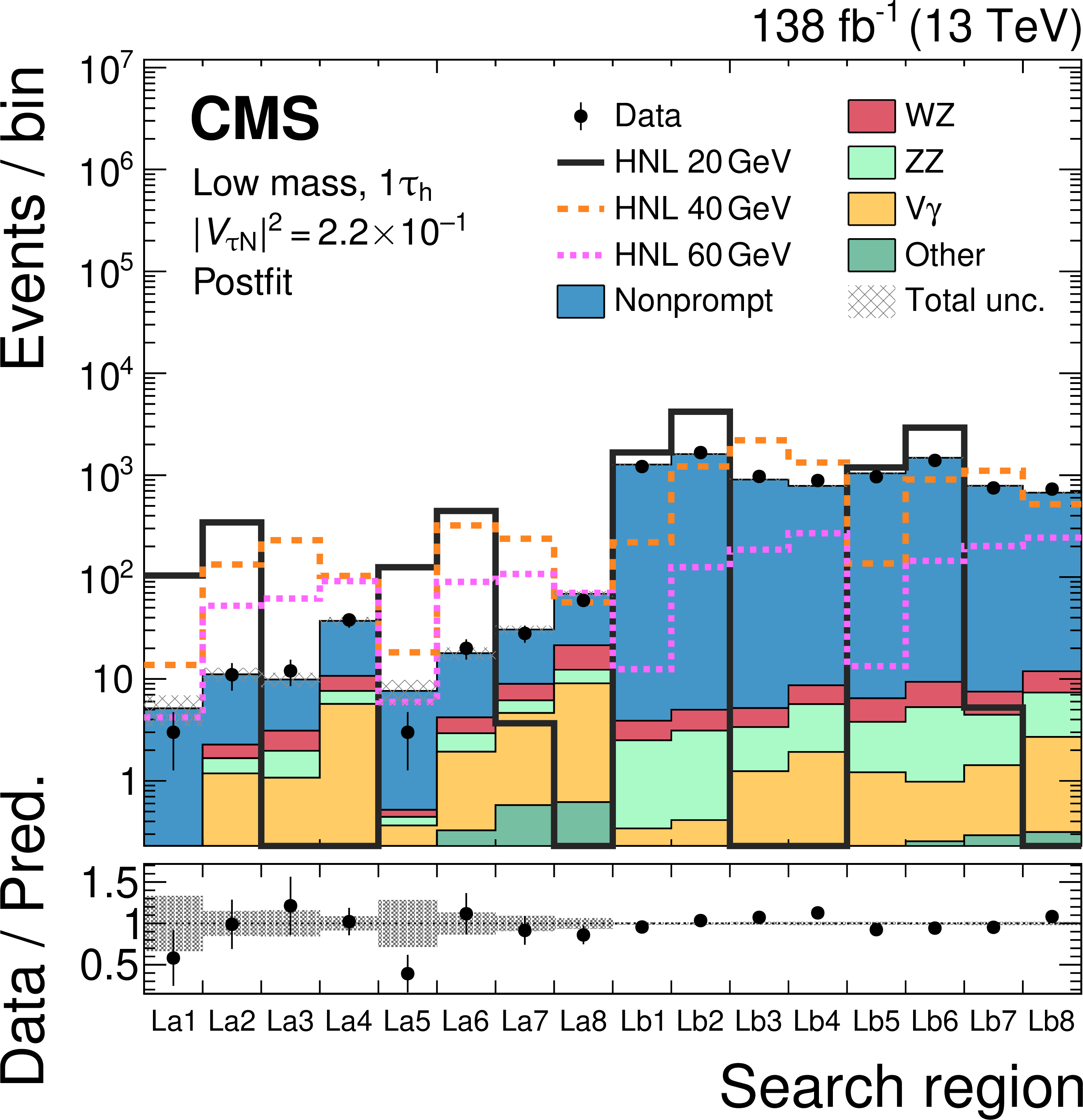
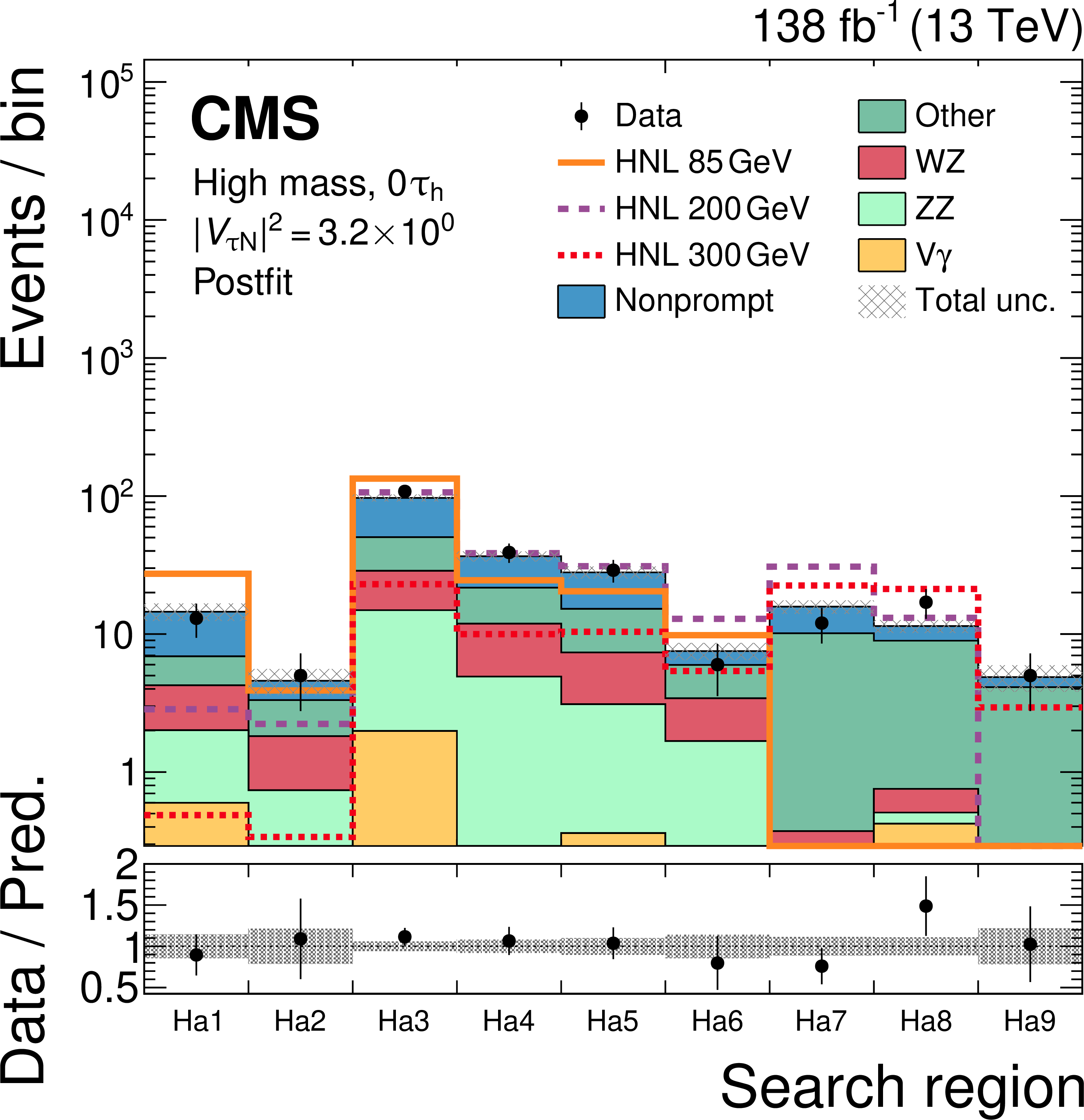
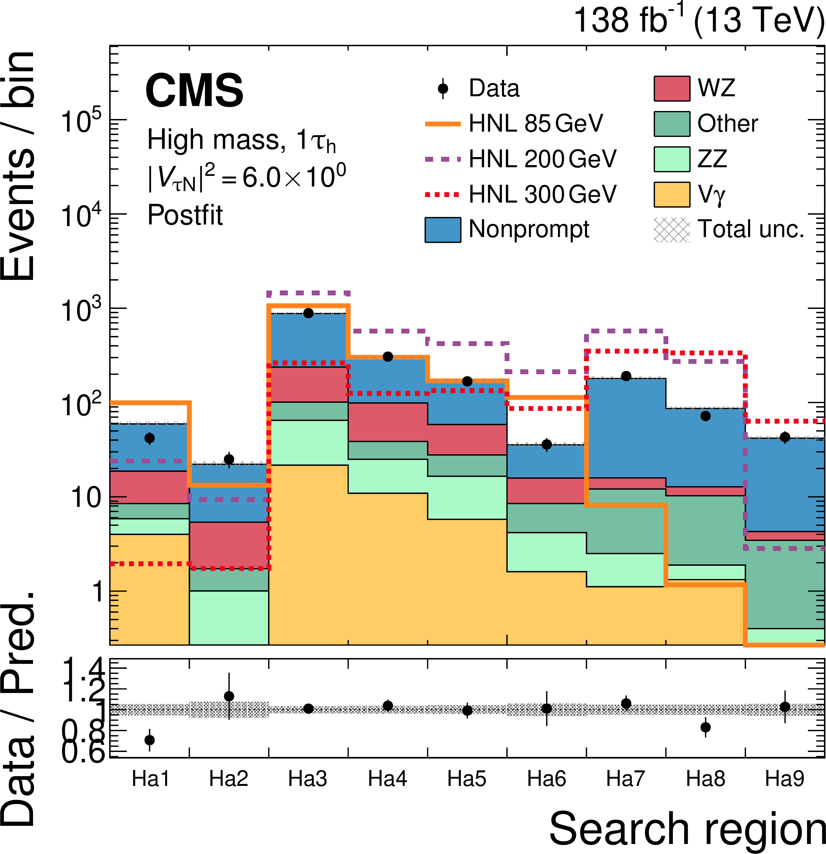
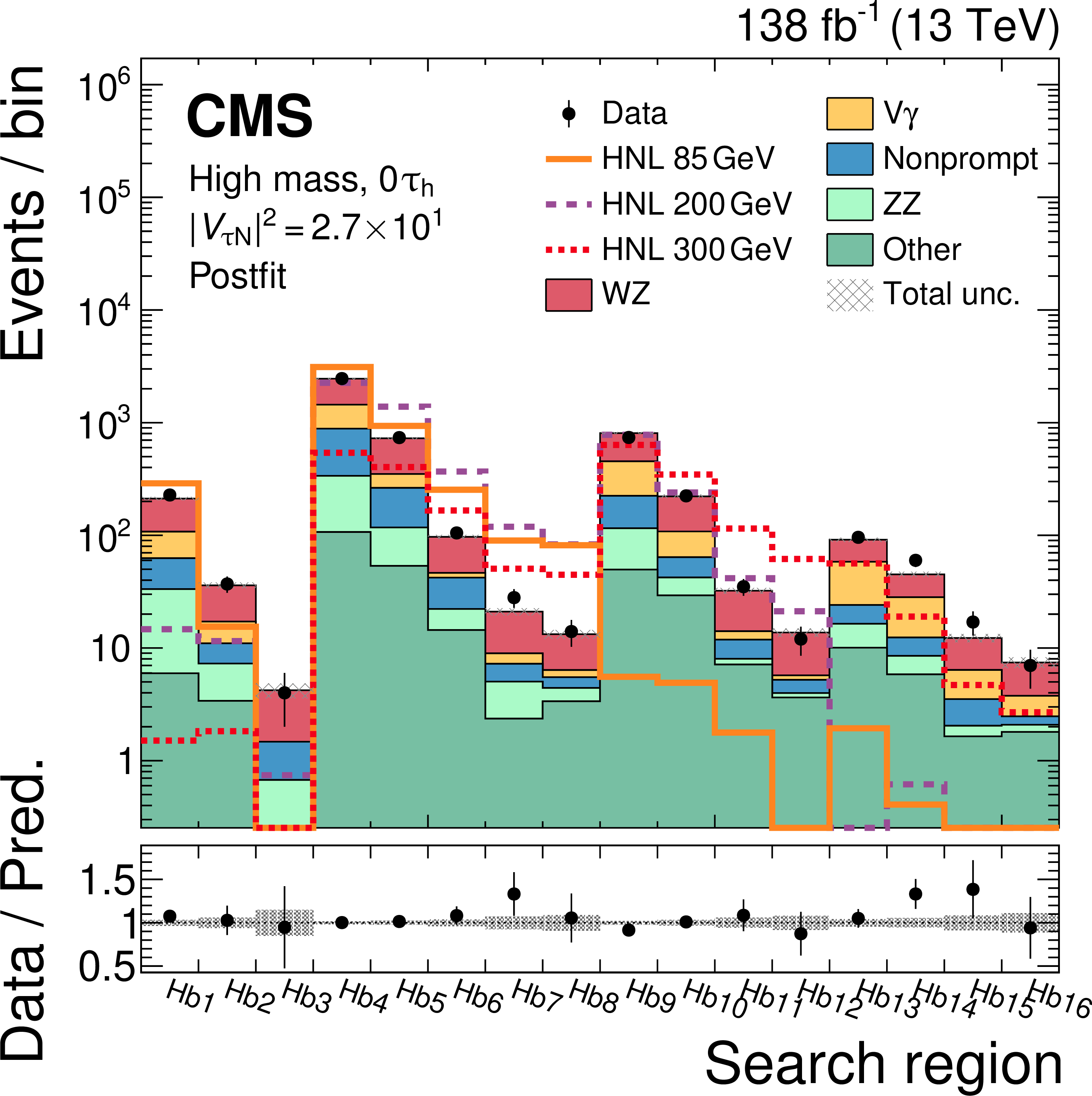
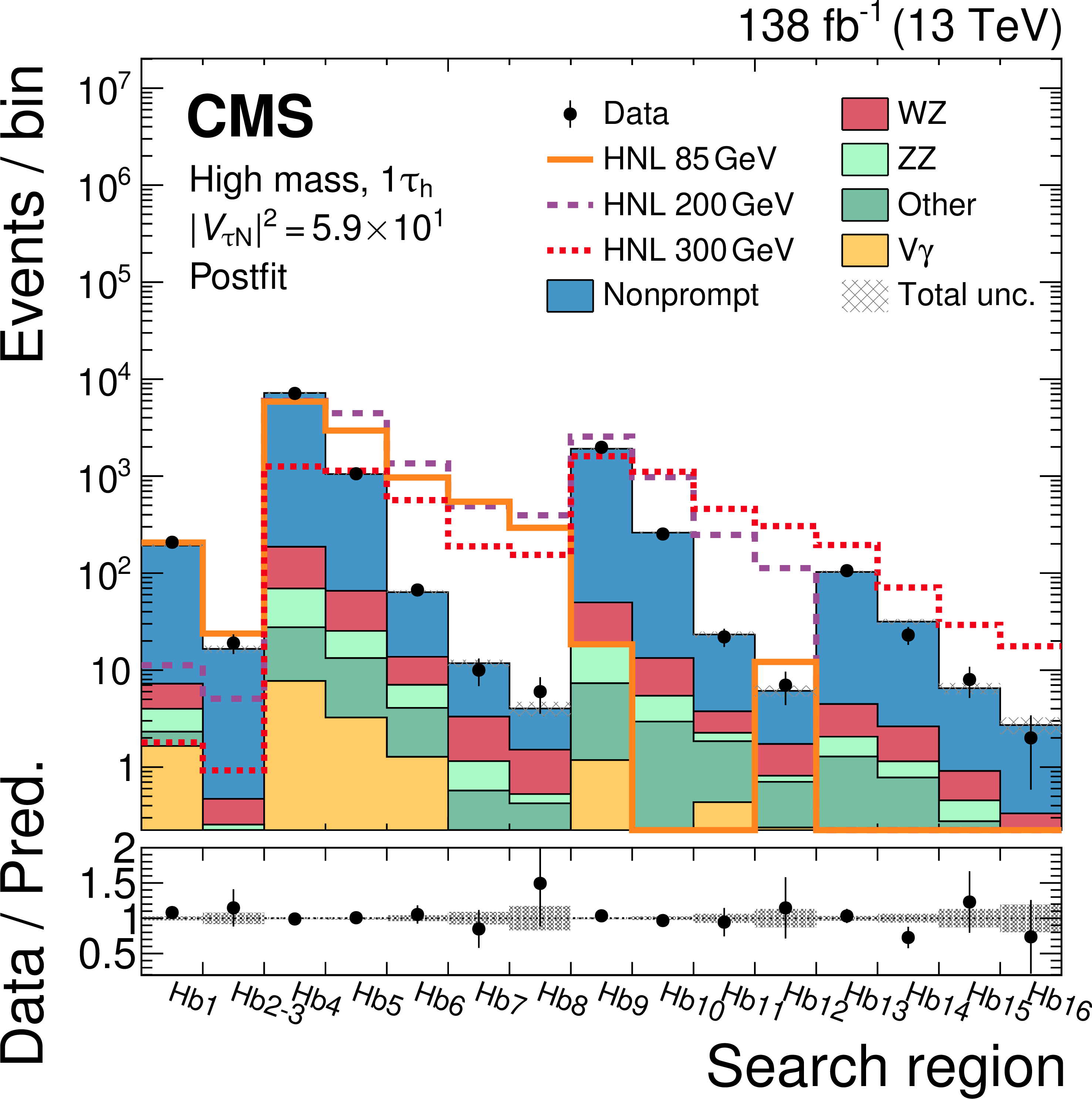
Figure 8:
Comparison of the number of observed (points) and predicted (coloured histograms) events in the SR bins, shown for the 0$ {\tau}{\mathrm{h}} $ (left column) and 1$ {\tau}{\mathrm{h}} $ (right column) categories combined. The La1-8 and Lb1-8 (upper row), Ha1-Ha9 (middle row), and Hb1-16 (lower row) are displayed. The predicted background yields are shown with the values of the normalizations and nuisance parameters obtained in background-only fits applied (``postfit''). The HNL predictions for three different $ m_{\mathrm{N}} $ values with exclusive coupling to tau neutrinos are shown with coloured lines. The vertical bars on the points represent the statistical uncertainties in the data, and the hatched bands the total uncertainties in the background predictions as obtained from the fits. In the lower panels, the ratios of the event yield in data to the overall sum of the background predictions are shown. |
png pdf |
Figure 8-a:
Comparison of the number of observed (points) and predicted (coloured histograms) events in the SR bins, shown for the 0$ {\tau}{\mathrm{h}} $ (left column) and 1$ {\tau}{\mathrm{h}} $ (right column) categories combined. The La1-8 and Lb1-8 (upper row), Ha1-Ha9 (middle row), and Hb1-16 (lower row) are displayed. The predicted background yields are shown with the values of the normalizations and nuisance parameters obtained in background-only fits applied (``postfit''). The HNL predictions for three different $ m_{\mathrm{N}} $ values with exclusive coupling to tau neutrinos are shown with coloured lines. The vertical bars on the points represent the statistical uncertainties in the data, and the hatched bands the total uncertainties in the background predictions as obtained from the fits. In the lower panels, the ratios of the event yield in data to the overall sum of the background predictions are shown. |
png pdf |
Figure 8-b:
Comparison of the number of observed (points) and predicted (coloured histograms) events in the SR bins, shown for the 0$ {\tau}{\mathrm{h}} $ (left column) and 1$ {\tau}{\mathrm{h}} $ (right column) categories combined. The La1-8 and Lb1-8 (upper row), Ha1-Ha9 (middle row), and Hb1-16 (lower row) are displayed. The predicted background yields are shown with the values of the normalizations and nuisance parameters obtained in background-only fits applied (``postfit''). The HNL predictions for three different $ m_{\mathrm{N}} $ values with exclusive coupling to tau neutrinos are shown with coloured lines. The vertical bars on the points represent the statistical uncertainties in the data, and the hatched bands the total uncertainties in the background predictions as obtained from the fits. In the lower panels, the ratios of the event yield in data to the overall sum of the background predictions are shown. |
png pdf |
Figure 8-c:
Comparison of the number of observed (points) and predicted (coloured histograms) events in the SR bins, shown for the 0$ {\tau}{\mathrm{h}} $ (left column) and 1$ {\tau}{\mathrm{h}} $ (right column) categories combined. The La1-8 and Lb1-8 (upper row), Ha1-Ha9 (middle row), and Hb1-16 (lower row) are displayed. The predicted background yields are shown with the values of the normalizations and nuisance parameters obtained in background-only fits applied (``postfit''). The HNL predictions for three different $ m_{\mathrm{N}} $ values with exclusive coupling to tau neutrinos are shown with coloured lines. The vertical bars on the points represent the statistical uncertainties in the data, and the hatched bands the total uncertainties in the background predictions as obtained from the fits. In the lower panels, the ratios of the event yield in data to the overall sum of the background predictions are shown. |
png pdf |
Figure 8-d:
Comparison of the number of observed (points) and predicted (coloured histograms) events in the SR bins, shown for the 0$ {\tau}{\mathrm{h}} $ (left column) and 1$ {\tau}{\mathrm{h}} $ (right column) categories combined. The La1-8 and Lb1-8 (upper row), Ha1-Ha9 (middle row), and Hb1-16 (lower row) are displayed. The predicted background yields are shown with the values of the normalizations and nuisance parameters obtained in background-only fits applied (``postfit''). The HNL predictions for three different $ m_{\mathrm{N}} $ values with exclusive coupling to tau neutrinos are shown with coloured lines. The vertical bars on the points represent the statistical uncertainties in the data, and the hatched bands the total uncertainties in the background predictions as obtained from the fits. In the lower panels, the ratios of the event yield in data to the overall sum of the background predictions are shown. |
png pdf |
Figure 8-e:
Comparison of the number of observed (points) and predicted (coloured histograms) events in the SR bins, shown for the 0$ {\tau}{\mathrm{h}} $ (left column) and 1$ {\tau}{\mathrm{h}} $ (right column) categories combined. The La1-8 and Lb1-8 (upper row), Ha1-Ha9 (middle row), and Hb1-16 (lower row) are displayed. The predicted background yields are shown with the values of the normalizations and nuisance parameters obtained in background-only fits applied (``postfit''). The HNL predictions for three different $ m_{\mathrm{N}} $ values with exclusive coupling to tau neutrinos are shown with coloured lines. The vertical bars on the points represent the statistical uncertainties in the data, and the hatched bands the total uncertainties in the background predictions as obtained from the fits. In the lower panels, the ratios of the event yield in data to the overall sum of the background predictions are shown. |
png pdf |
Figure 8-f:
Comparison of the number of observed (points) and predicted (coloured histograms) events in the SR bins, shown for the 0$ {\tau}{\mathrm{h}} $ (left column) and 1$ {\tau}{\mathrm{h}} $ (right column) categories combined. The La1-8 and Lb1-8 (upper row), Ha1-Ha9 (middle row), and Hb1-16 (lower row) are displayed. The predicted background yields are shown with the values of the normalizations and nuisance parameters obtained in background-only fits applied (``postfit''). The HNL predictions for three different $ m_{\mathrm{N}} $ values with exclusive coupling to tau neutrinos are shown with coloured lines. The vertical bars on the points represent the statistical uncertainties in the data, and the hatched bands the total uncertainties in the background predictions as obtained from the fits. In the lower panels, the ratios of the event yield in data to the overall sum of the background predictions are shown. |
png pdf |
Figure 9:
Comparison of the observed (points) and predicted (coloured histograms) BDT output distributions of the low-mass selection, shown for the $ \mathrm{e}\mathrm{e}\mathrm{e} $ and $ \mathrm{e}\mathrm{e}\mu $ channels combined (left column) and the $ \mathrm{e}\mu\mu $ and $ \mu\mu\mu $ channels combined (right column). The output scores BDT(10-40, e, 0$ {\tau}{\mathrm{h}} $) (upper left), BDT(10-40, $ \mu $, 0$ {\tau}{\mathrm{h}} $) (upper right), BDT(50-75, e, 0$ {\tau}{\mathrm{h}} $) (lower left), and BDT(50-75, $ \mu $, 0$ {\tau}{\mathrm{h}} $) (lower right) are displayed. The predicted background yields are shown with the values of the normalizations and nuisance parameters obtained in background-only fits applied (``postfit''). The HNL predictions for three different $ m_{\mathrm{N}} $ values with exclusive coupling to electron (left column) or muon (right column) neutrinos are shown with coloured lines. The vertical bars on the points represent the statistical uncertainties in the data, and the hatched bands the total uncertainties in the background predictions as obtained from the fits. In the lower panels, the ratios of the event yield in data to the overall sum of the background predictions are shown. |
png pdf |
Figure 9-a:
Comparison of the observed (points) and predicted (coloured histograms) BDT output distributions of the low-mass selection, shown for the $ \mathrm{e}\mathrm{e}\mathrm{e} $ and $ \mathrm{e}\mathrm{e}\mu $ channels combined (left column) and the $ \mathrm{e}\mu\mu $ and $ \mu\mu\mu $ channels combined (right column). The output scores BDT(10-40, e, 0$ {\tau}{\mathrm{h}} $) (upper left), BDT(10-40, $ \mu $, 0$ {\tau}{\mathrm{h}} $) (upper right), BDT(50-75, e, 0$ {\tau}{\mathrm{h}} $) (lower left), and BDT(50-75, $ \mu $, 0$ {\tau}{\mathrm{h}} $) (lower right) are displayed. The predicted background yields are shown with the values of the normalizations and nuisance parameters obtained in background-only fits applied (``postfit''). The HNL predictions for three different $ m_{\mathrm{N}} $ values with exclusive coupling to electron (left column) or muon (right column) neutrinos are shown with coloured lines. The vertical bars on the points represent the statistical uncertainties in the data, and the hatched bands the total uncertainties in the background predictions as obtained from the fits. In the lower panels, the ratios of the event yield in data to the overall sum of the background predictions are shown. |
png pdf |
Figure 9-b:
Comparison of the observed (points) and predicted (coloured histograms) BDT output distributions of the low-mass selection, shown for the $ \mathrm{e}\mathrm{e}\mathrm{e} $ and $ \mathrm{e}\mathrm{e}\mu $ channels combined (left column) and the $ \mathrm{e}\mu\mu $ and $ \mu\mu\mu $ channels combined (right column). The output scores BDT(10-40, e, 0$ {\tau}{\mathrm{h}} $) (upper left), BDT(10-40, $ \mu $, 0$ {\tau}{\mathrm{h}} $) (upper right), BDT(50-75, e, 0$ {\tau}{\mathrm{h}} $) (lower left), and BDT(50-75, $ \mu $, 0$ {\tau}{\mathrm{h}} $) (lower right) are displayed. The predicted background yields are shown with the values of the normalizations and nuisance parameters obtained in background-only fits applied (``postfit''). The HNL predictions for three different $ m_{\mathrm{N}} $ values with exclusive coupling to electron (left column) or muon (right column) neutrinos are shown with coloured lines. The vertical bars on the points represent the statistical uncertainties in the data, and the hatched bands the total uncertainties in the background predictions as obtained from the fits. In the lower panels, the ratios of the event yield in data to the overall sum of the background predictions are shown. |
png pdf |
Figure 9-c:
Comparison of the observed (points) and predicted (coloured histograms) BDT output distributions of the low-mass selection, shown for the $ \mathrm{e}\mathrm{e}\mathrm{e} $ and $ \mathrm{e}\mathrm{e}\mu $ channels combined (left column) and the $ \mathrm{e}\mu\mu $ and $ \mu\mu\mu $ channels combined (right column). The output scores BDT(10-40, e, 0$ {\tau}{\mathrm{h}} $) (upper left), BDT(10-40, $ \mu $, 0$ {\tau}{\mathrm{h}} $) (upper right), BDT(50-75, e, 0$ {\tau}{\mathrm{h}} $) (lower left), and BDT(50-75, $ \mu $, 0$ {\tau}{\mathrm{h}} $) (lower right) are displayed. The predicted background yields are shown with the values of the normalizations and nuisance parameters obtained in background-only fits applied (``postfit''). The HNL predictions for three different $ m_{\mathrm{N}} $ values with exclusive coupling to electron (left column) or muon (right column) neutrinos are shown with coloured lines. The vertical bars on the points represent the statistical uncertainties in the data, and the hatched bands the total uncertainties in the background predictions as obtained from the fits. In the lower panels, the ratios of the event yield in data to the overall sum of the background predictions are shown. |
png pdf |
Figure 9-d:
Comparison of the observed (points) and predicted (coloured histograms) BDT output distributions of the low-mass selection, shown for the $ \mathrm{e}\mathrm{e}\mathrm{e} $ and $ \mathrm{e}\mathrm{e}\mu $ channels combined (left column) and the $ \mathrm{e}\mu\mu $ and $ \mu\mu\mu $ channels combined (right column). The output scores BDT(10-40, e, 0$ {\tau}{\mathrm{h}} $) (upper left), BDT(10-40, $ \mu $, 0$ {\tau}{\mathrm{h}} $) (upper right), BDT(50-75, e, 0$ {\tau}{\mathrm{h}} $) (lower left), and BDT(50-75, $ \mu $, 0$ {\tau}{\mathrm{h}} $) (lower right) are displayed. The predicted background yields are shown with the values of the normalizations and nuisance parameters obtained in background-only fits applied (``postfit''). The HNL predictions for three different $ m_{\mathrm{N}} $ values with exclusive coupling to electron (left column) or muon (right column) neutrinos are shown with coloured lines. The vertical bars on the points represent the statistical uncertainties in the data, and the hatched bands the total uncertainties in the background predictions as obtained from the fits. In the lower panels, the ratios of the event yield in data to the overall sum of the background predictions are shown. |
png pdf |
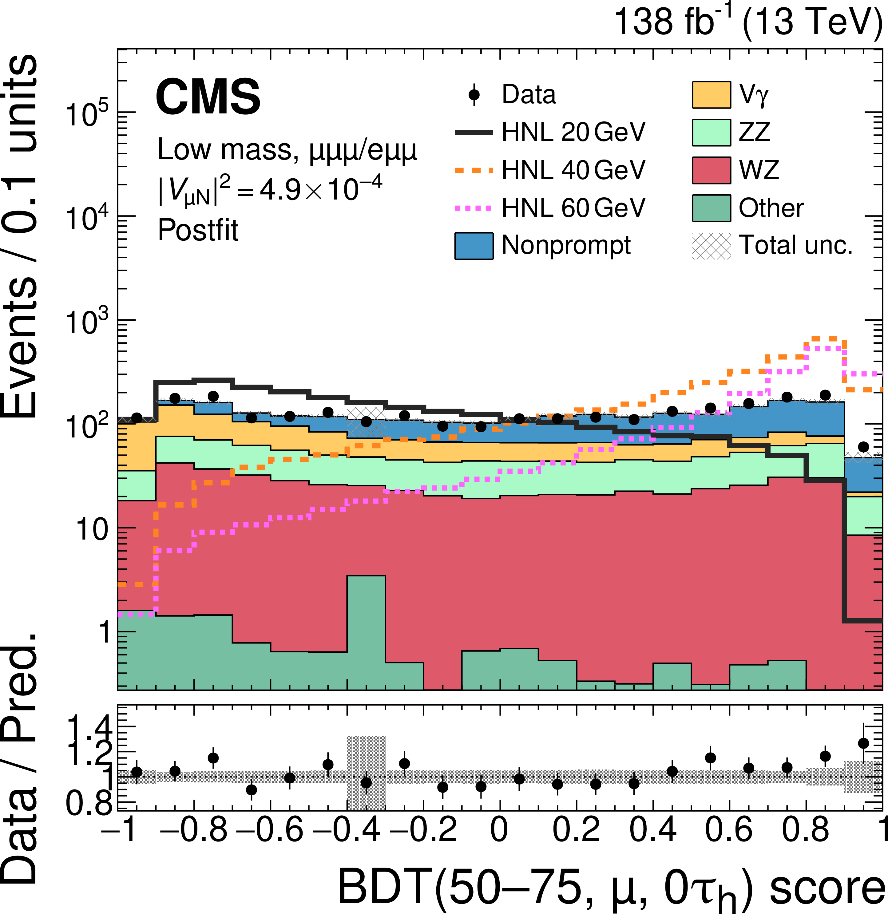
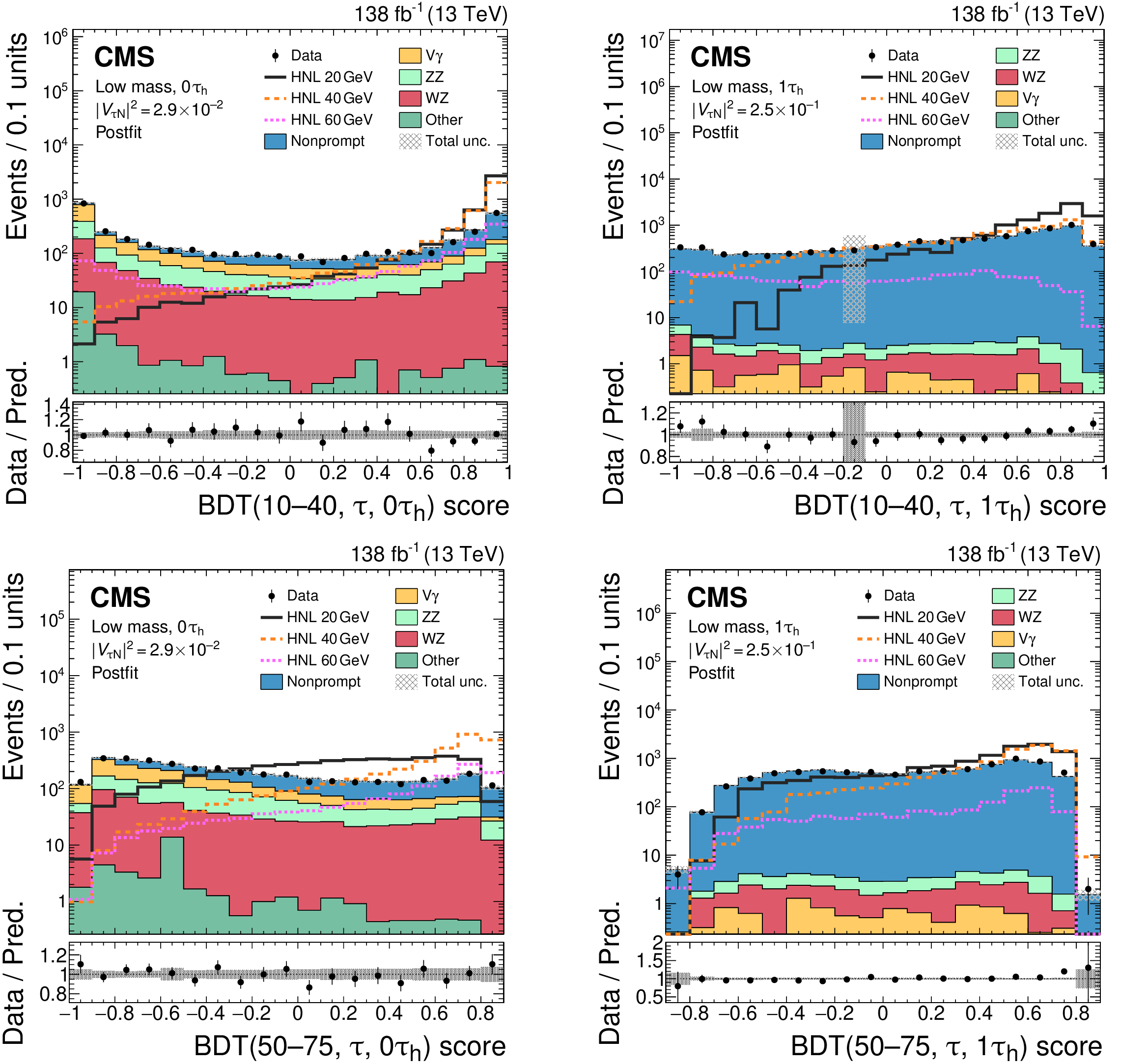
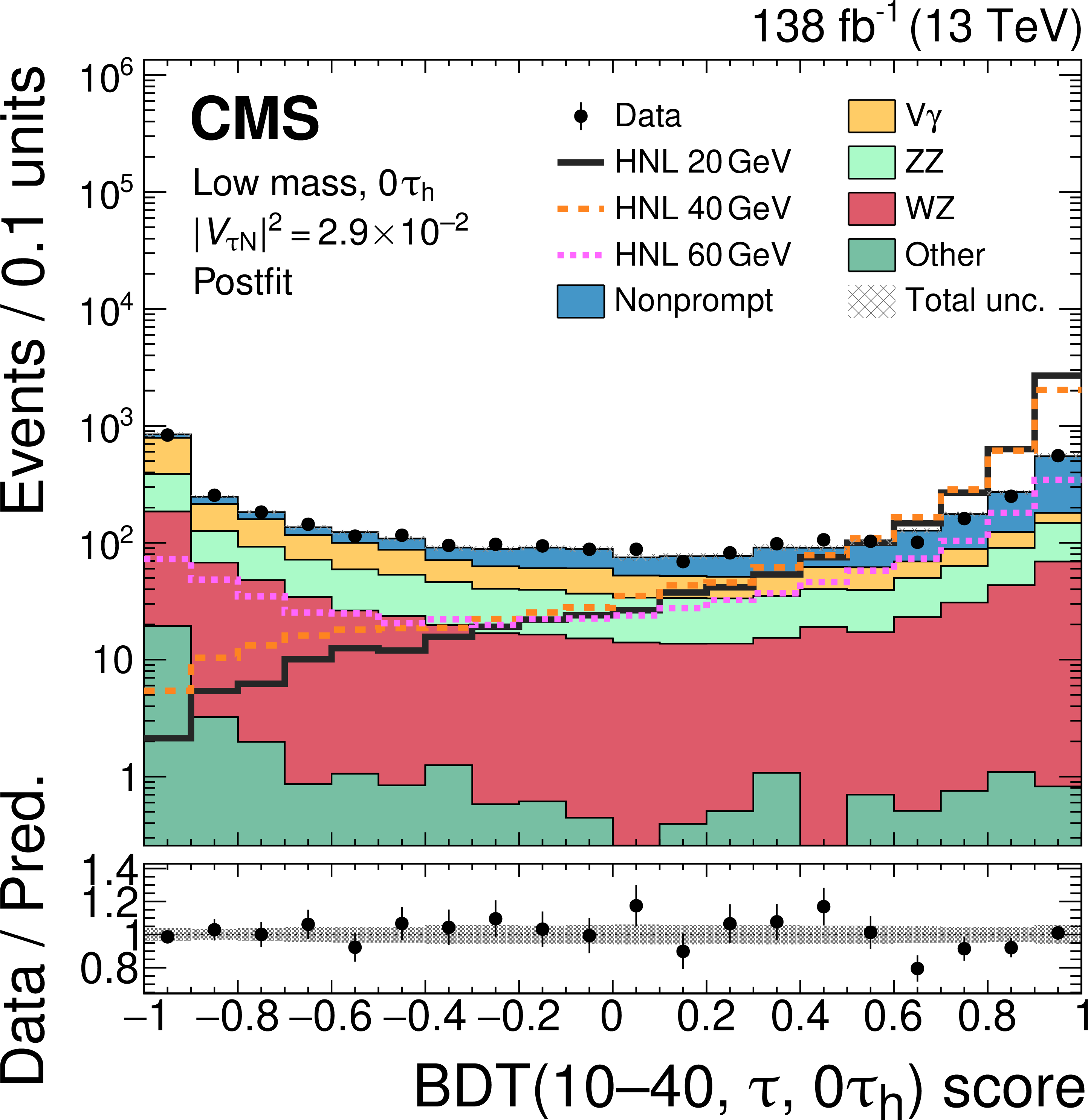
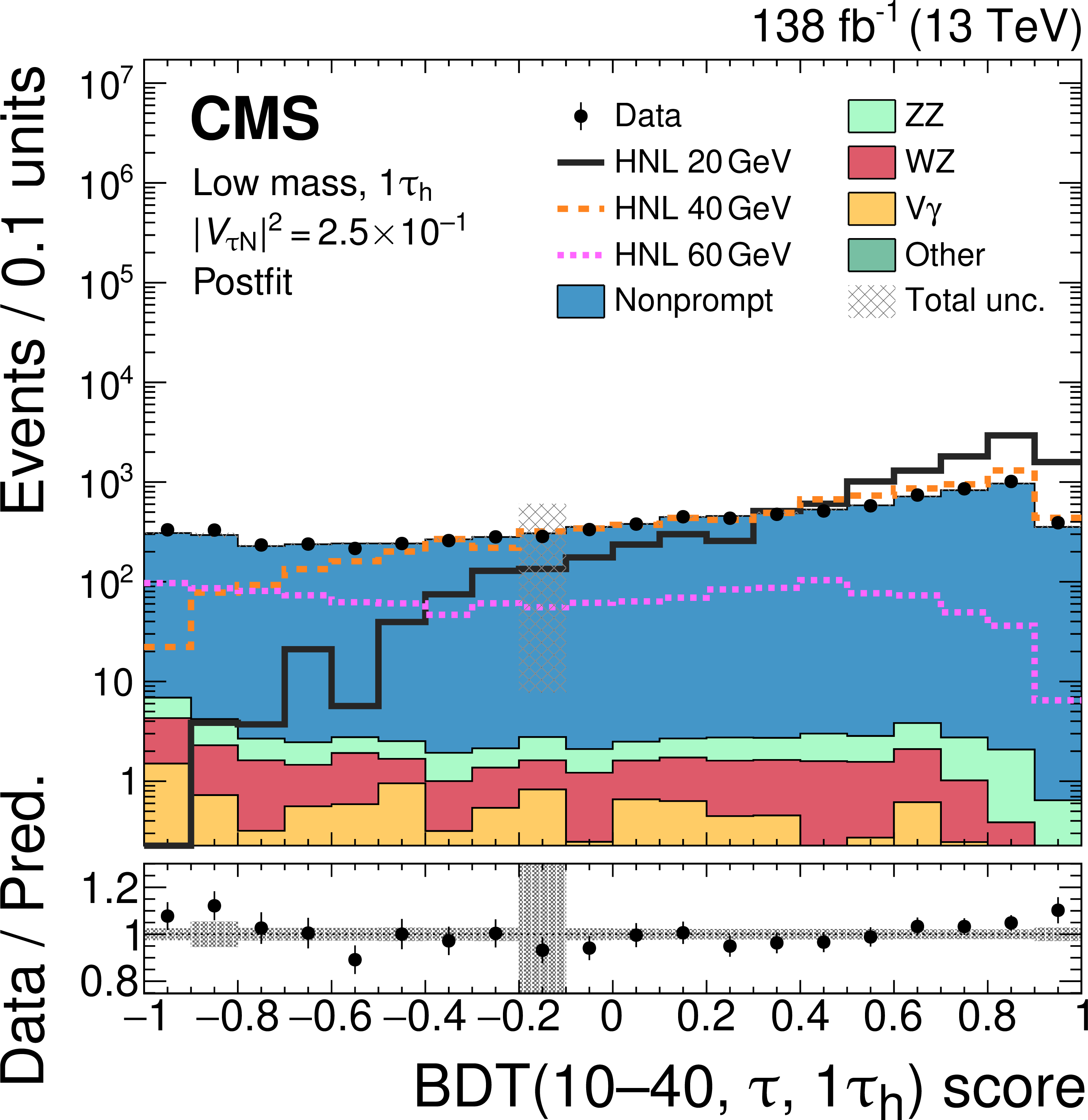
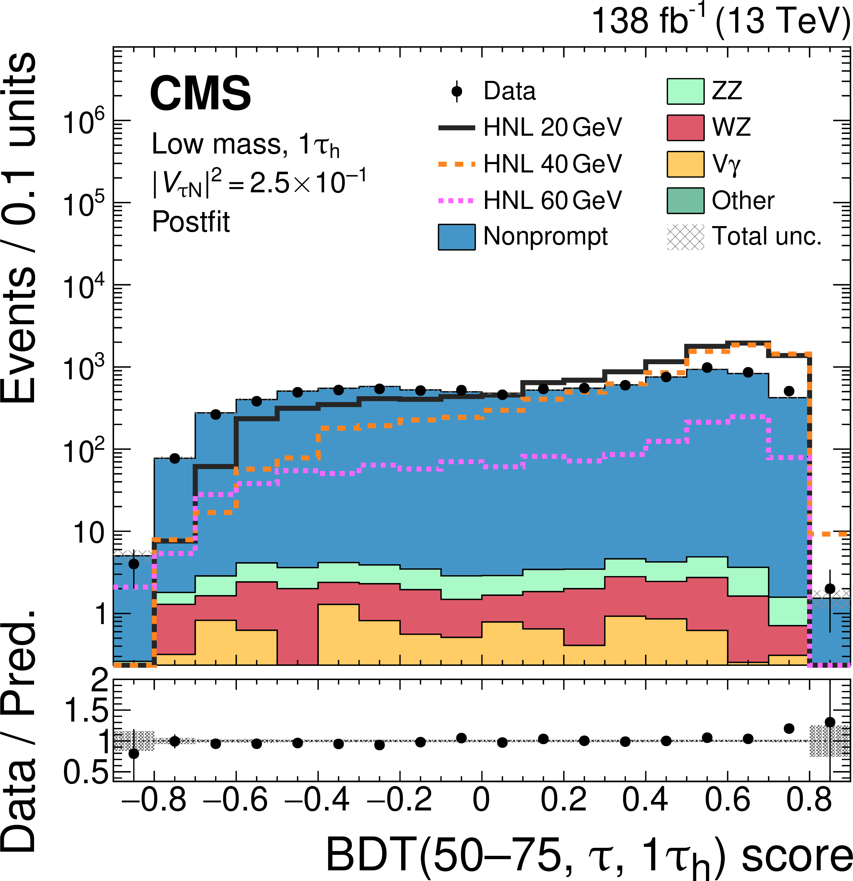
Figure 10:
Comparison of the observed (points) and predicted (coloured histograms) BDT output distributions of the low-mass selection, shown for the 0$ {\tau}{\mathrm{h}} $ channels combined (left column) and the 1$ {\tau}{\mathrm{h}} $ channels combined (right column). The output scores BDT(10-40, $ \tau $, 0$ {\tau}{\mathrm{h}} $) (upper left), BDT(10-40, $ \tau $, 1$ {\tau}{\mathrm{h}} $) (upper right), BDT(50-75, $ \tau $, 0$ {\tau}{\mathrm{h}} $) (lower left), and BDT(50-75, $ \tau $, 0$ {\tau}{\mathrm{h}} $) (lower right) are displayed. The predicted background yields are shown with the values of the normalizations and nuisance parameters obtained in background-only fits applied (``postfit''). The HNL predictions for three different $ m_{\mathrm{N}} $ values with exclusive coupling to tau neutrinos are shown with coloured lines. The vertical bars on the points represent the statistical uncertainties in the data, and the hatched bands the total uncertainties in the background predictions as obtained from the fits. In the lower panels, the ratios of the event yield in data to the overall sum of the background predictions are shown. |
png pdf |
Figure 10-a:
Comparison of the observed (points) and predicted (coloured histograms) BDT output distributions of the low-mass selection, shown for the 0$ {\tau}{\mathrm{h}} $ channels combined (left column) and the 1$ {\tau}{\mathrm{h}} $ channels combined (right column). The output scores BDT(10-40, $ \tau $, 0$ {\tau}{\mathrm{h}} $) (upper left), BDT(10-40, $ \tau $, 1$ {\tau}{\mathrm{h}} $) (upper right), BDT(50-75, $ \tau $, 0$ {\tau}{\mathrm{h}} $) (lower left), and BDT(50-75, $ \tau $, 0$ {\tau}{\mathrm{h}} $) (lower right) are displayed. The predicted background yields are shown with the values of the normalizations and nuisance parameters obtained in background-only fits applied (``postfit''). The HNL predictions for three different $ m_{\mathrm{N}} $ values with exclusive coupling to tau neutrinos are shown with coloured lines. The vertical bars on the points represent the statistical uncertainties in the data, and the hatched bands the total uncertainties in the background predictions as obtained from the fits. In the lower panels, the ratios of the event yield in data to the overall sum of the background predictions are shown. |
png pdf |
Figure 10-b:
Comparison of the observed (points) and predicted (coloured histograms) BDT output distributions of the low-mass selection, shown for the 0$ {\tau}{\mathrm{h}} $ channels combined (left column) and the 1$ {\tau}{\mathrm{h}} $ channels combined (right column). The output scores BDT(10-40, $ \tau $, 0$ {\tau}{\mathrm{h}} $) (upper left), BDT(10-40, $ \tau $, 1$ {\tau}{\mathrm{h}} $) (upper right), BDT(50-75, $ \tau $, 0$ {\tau}{\mathrm{h}} $) (lower left), and BDT(50-75, $ \tau $, 0$ {\tau}{\mathrm{h}} $) (lower right) are displayed. The predicted background yields are shown with the values of the normalizations and nuisance parameters obtained in background-only fits applied (``postfit''). The HNL predictions for three different $ m_{\mathrm{N}} $ values with exclusive coupling to tau neutrinos are shown with coloured lines. The vertical bars on the points represent the statistical uncertainties in the data, and the hatched bands the total uncertainties in the background predictions as obtained from the fits. In the lower panels, the ratios of the event yield in data to the overall sum of the background predictions are shown. |
png pdf |
Figure 10-c:
Comparison of the observed (points) and predicted (coloured histograms) BDT output distributions of the low-mass selection, shown for the 0$ {\tau}{\mathrm{h}} $ channels combined (left column) and the 1$ {\tau}{\mathrm{h}} $ channels combined (right column). The output scores BDT(10-40, $ \tau $, 0$ {\tau}{\mathrm{h}} $) (upper left), BDT(10-40, $ \tau $, 1$ {\tau}{\mathrm{h}} $) (upper right), BDT(50-75, $ \tau $, 0$ {\tau}{\mathrm{h}} $) (lower left), and BDT(50-75, $ \tau $, 0$ {\tau}{\mathrm{h}} $) (lower right) are displayed. The predicted background yields are shown with the values of the normalizations and nuisance parameters obtained in background-only fits applied (``postfit''). The HNL predictions for three different $ m_{\mathrm{N}} $ values with exclusive coupling to tau neutrinos are shown with coloured lines. The vertical bars on the points represent the statistical uncertainties in the data, and the hatched bands the total uncertainties in the background predictions as obtained from the fits. In the lower panels, the ratios of the event yield in data to the overall sum of the background predictions are shown. |
png pdf |
Figure 10-d:
Comparison of the observed (points) and predicted (coloured histograms) BDT output distributions of the low-mass selection, shown for the 0$ {\tau}{\mathrm{h}} $ channels combined (left column) and the 1$ {\tau}{\mathrm{h}} $ channels combined (right column). The output scores BDT(10-40, $ \tau $, 0$ {\tau}{\mathrm{h}} $) (upper left), BDT(10-40, $ \tau $, 1$ {\tau}{\mathrm{h}} $) (upper right), BDT(50-75, $ \tau $, 0$ {\tau}{\mathrm{h}} $) (lower left), and BDT(50-75, $ \tau $, 0$ {\tau}{\mathrm{h}} $) (lower right) are displayed. The predicted background yields are shown with the values of the normalizations and nuisance parameters obtained in background-only fits applied (``postfit''). The HNL predictions for three different $ m_{\mathrm{N}} $ values with exclusive coupling to tau neutrinos are shown with coloured lines. The vertical bars on the points represent the statistical uncertainties in the data, and the hatched bands the total uncertainties in the background predictions as obtained from the fits. In the lower panels, the ratios of the event yield in data to the overall sum of the background predictions are shown. |
png pdf |
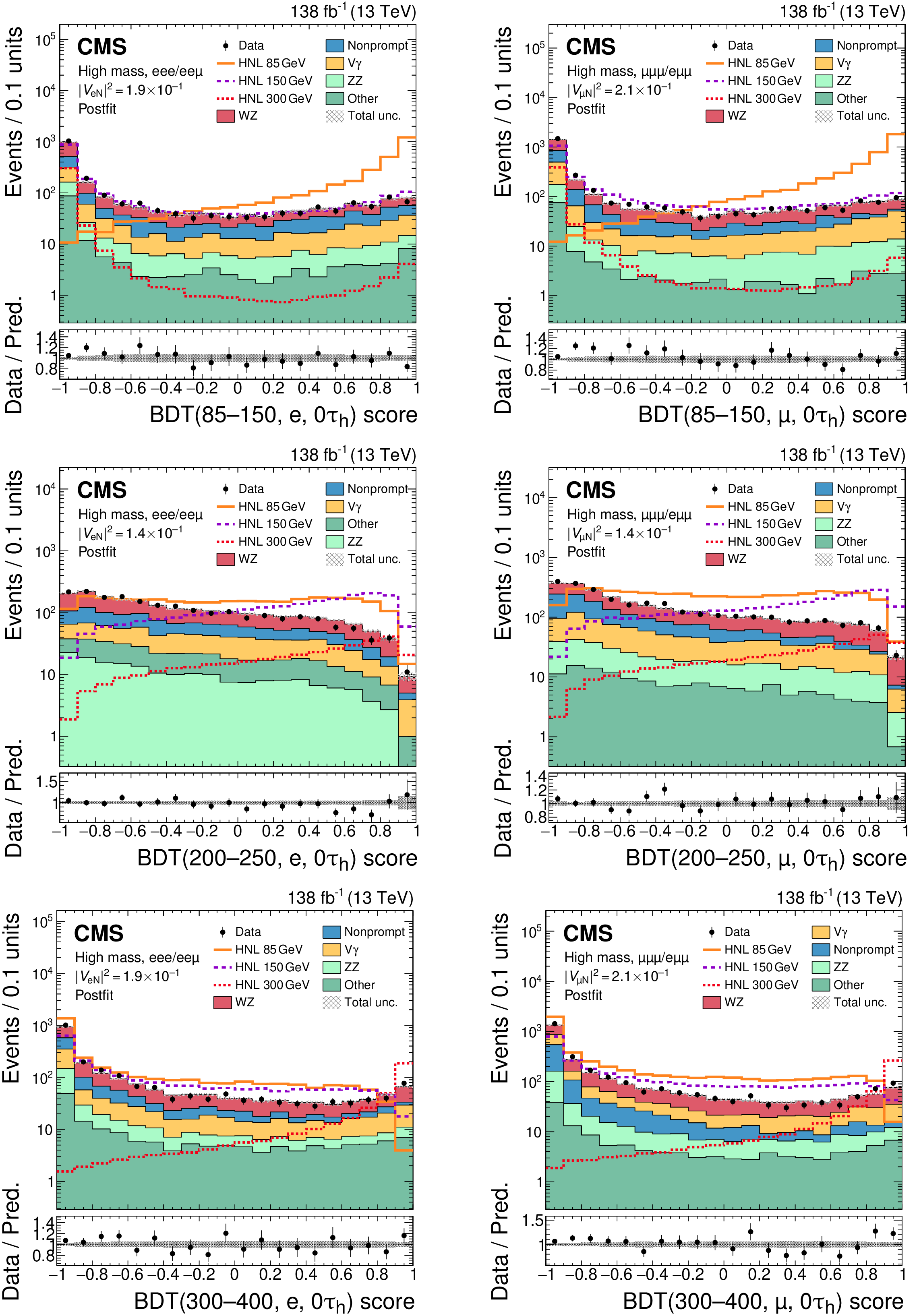
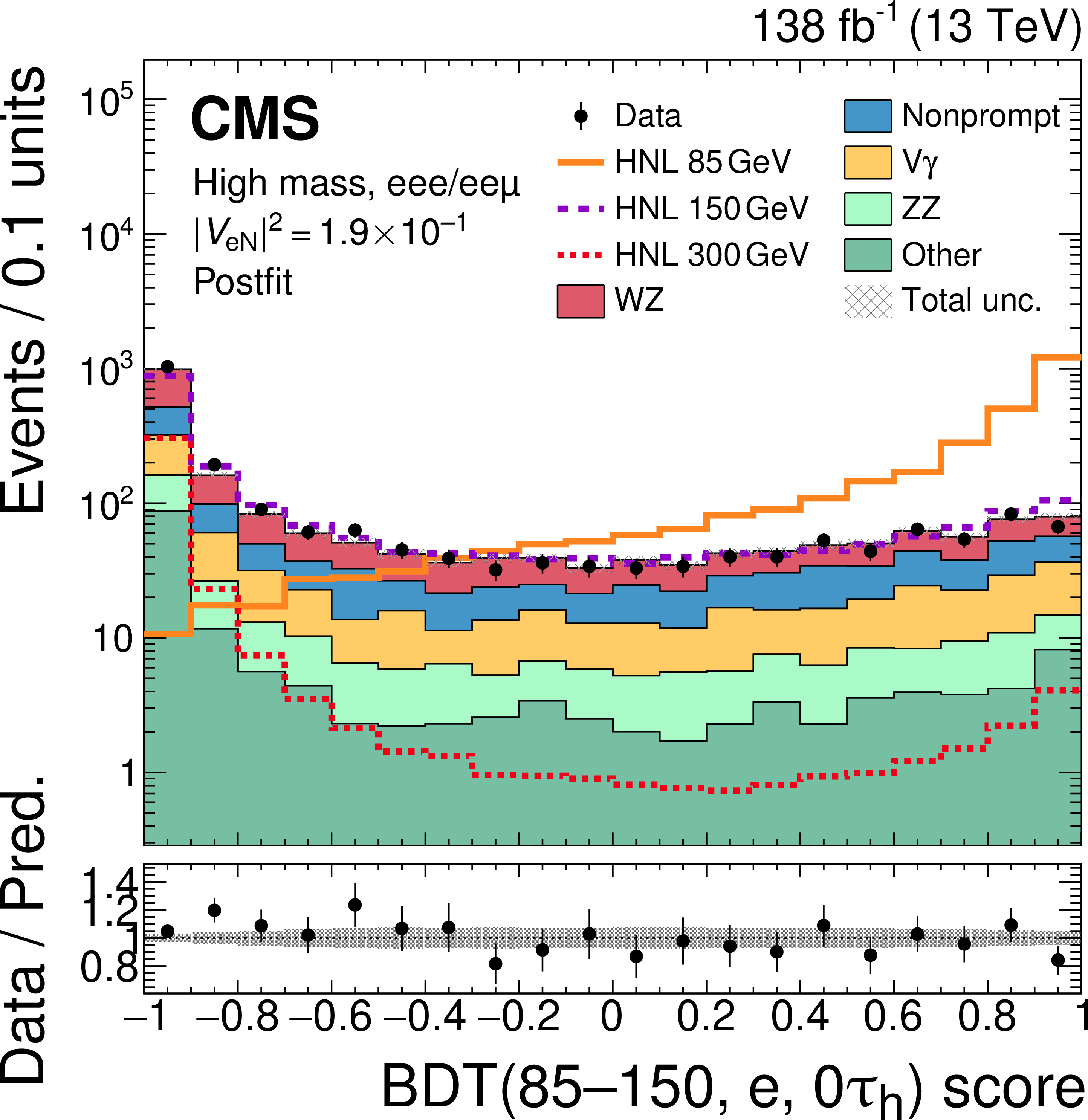
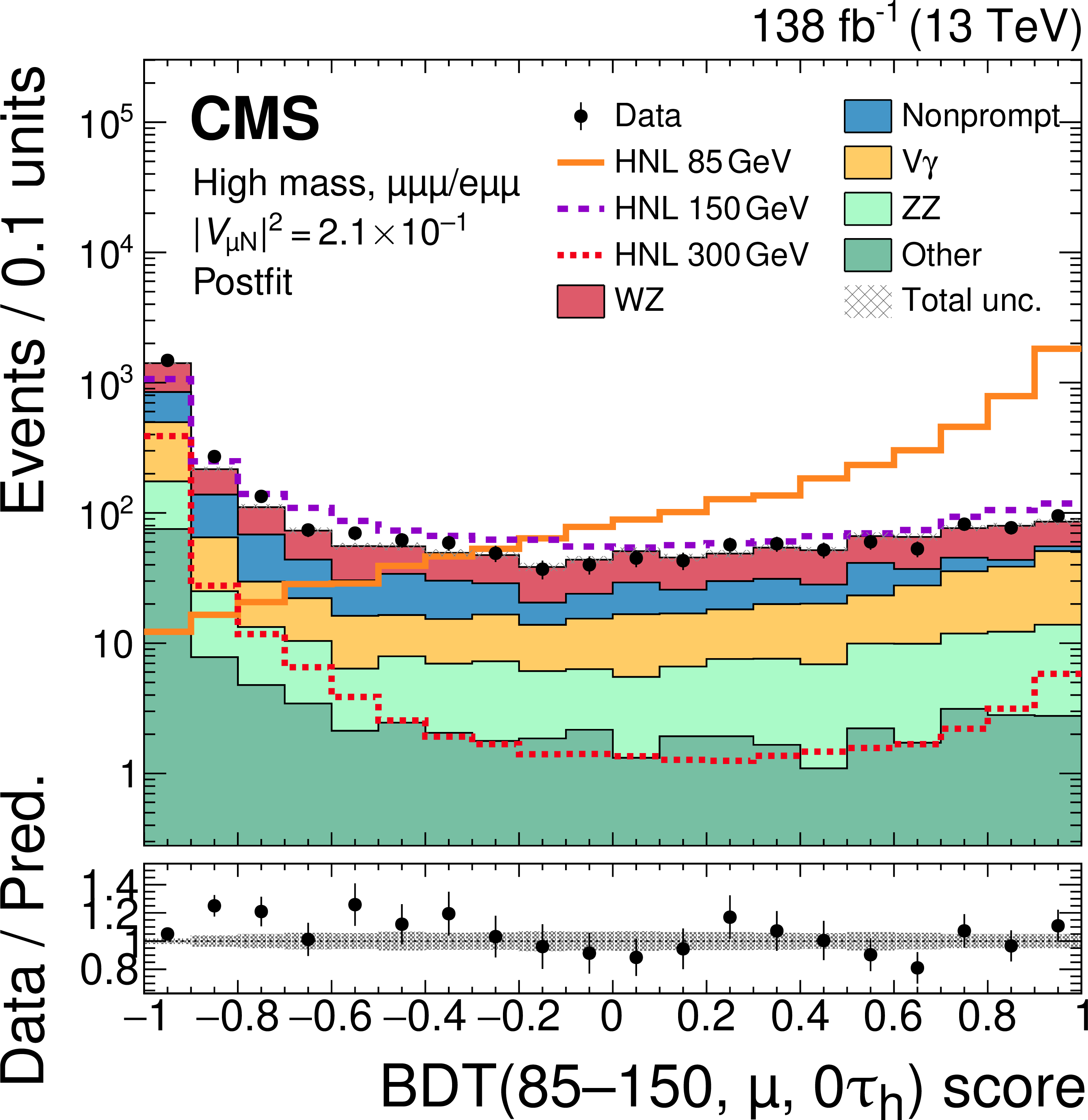
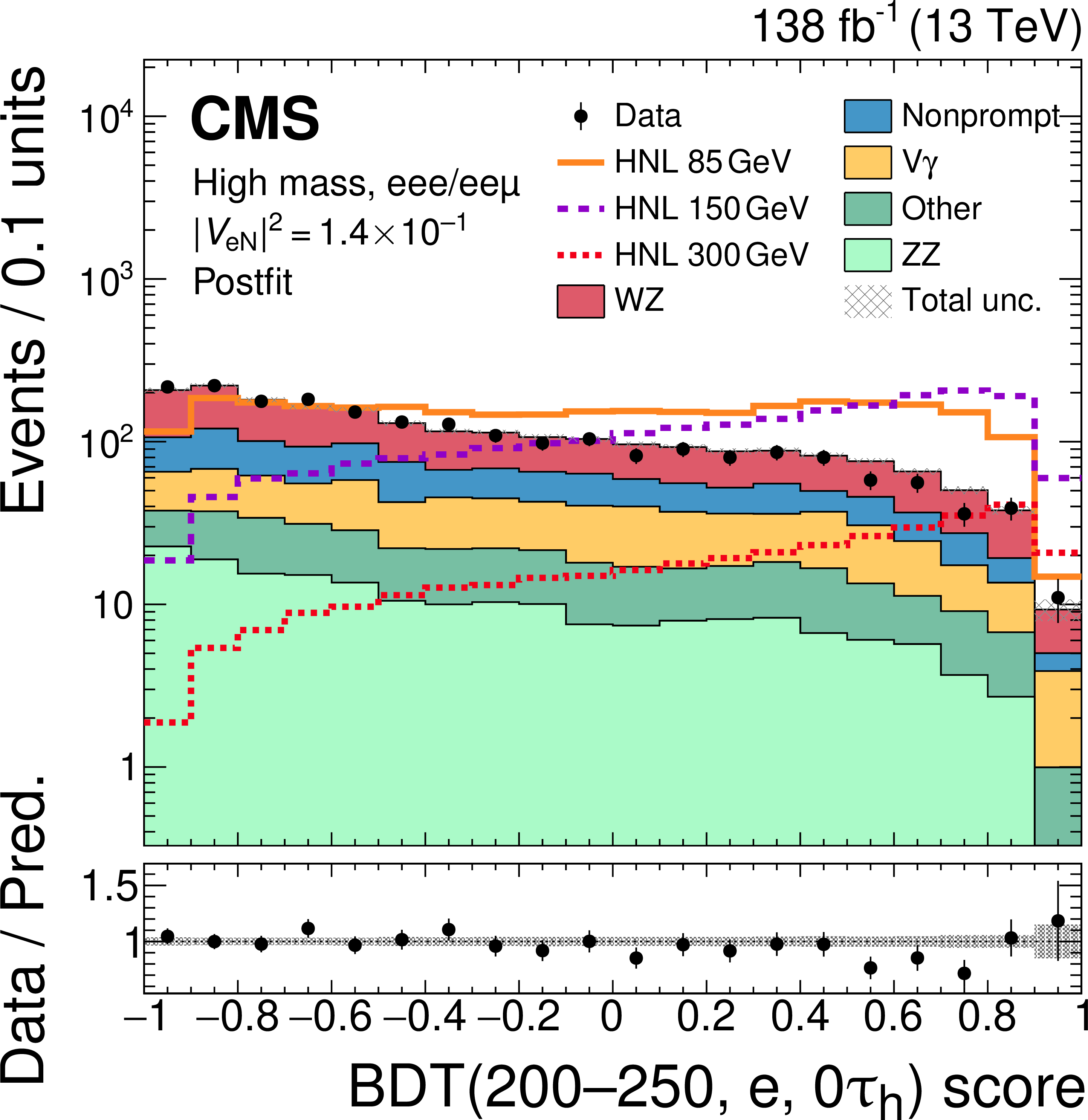
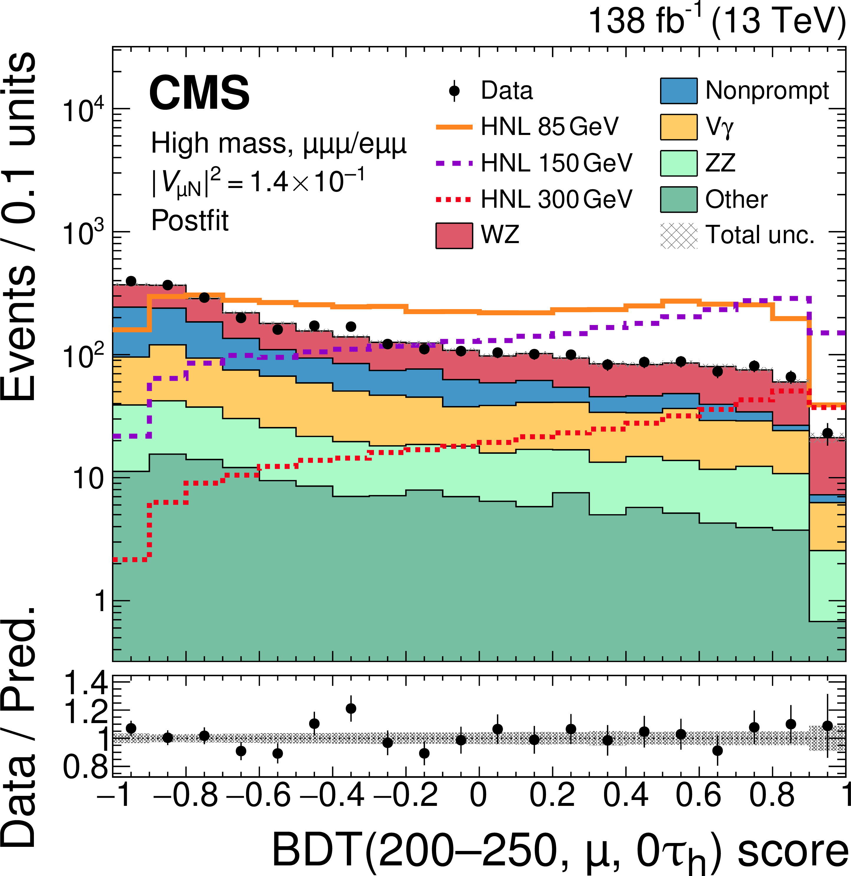
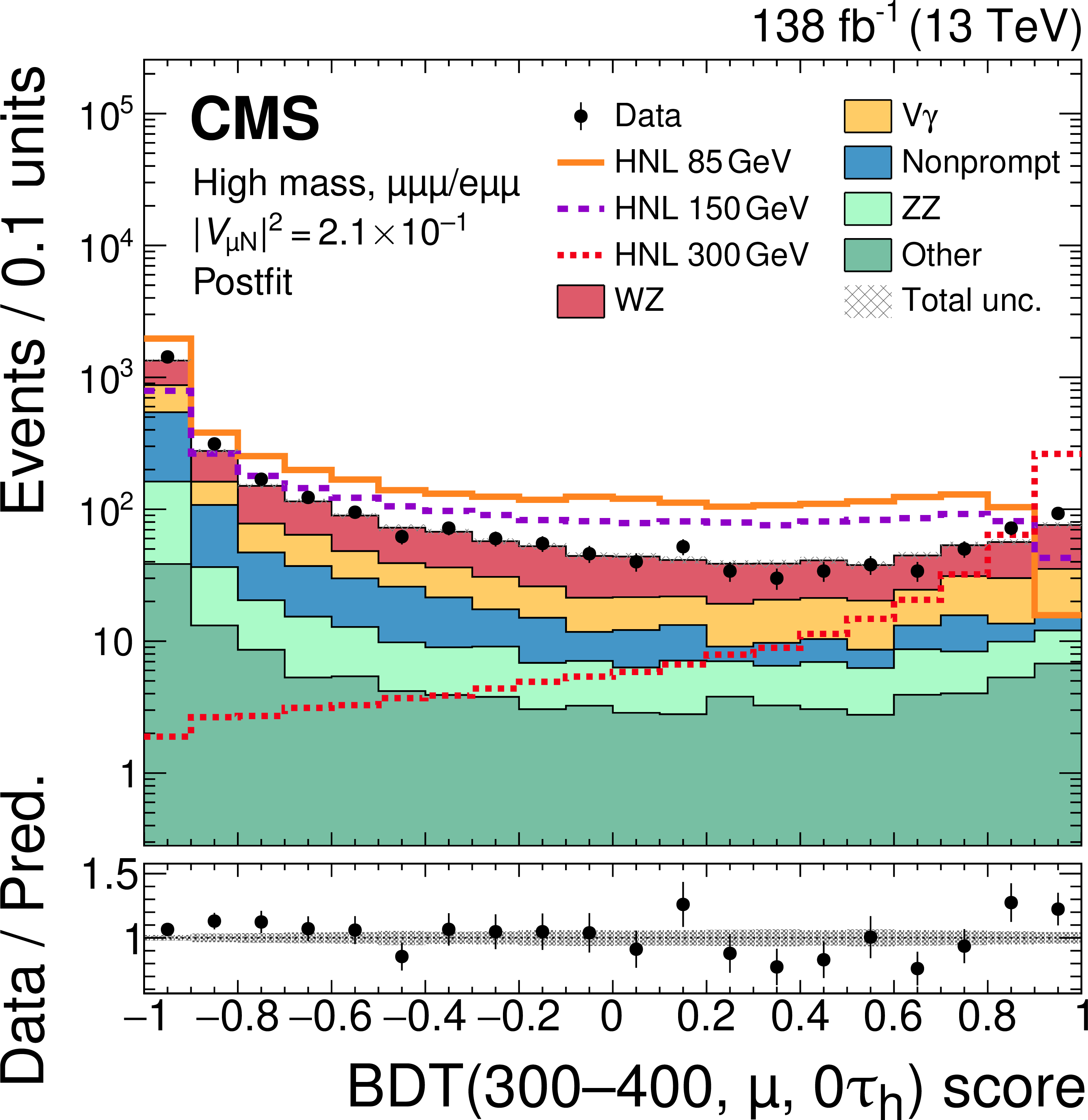
Figure 11:
Comparison of the observed (points) and predicted (coloured histograms) BDT output distributions of the high-mass selection, shown for the $ \mathrm{e}\mathrm{e}\mathrm{e} $ and $ \mathrm{e}\mathrm{e}\mu $ channels combined (left column) and the $ \mathrm{e}\mu\mu $ and $ \mu\mu\mu $ channels combined (right column). The output scores BDT(85-150, e, 0$ {\tau}{\mathrm{h}} $) (upper left), BDT(85-150, $ \mu $, 0$ {\tau}{\mathrm{h}} $) (upper right), BDT(200-250, e, 0$ {\tau}{\mathrm{h}} $) (middle left), BDT(200-250, $ \mu $, 0$ {\tau}{\mathrm{h}} $) (middle right), BDT(300-400, e, 0$ {\tau}{\mathrm{h}} $) (lower left), and BDT(300-400, $ \mu $, 0$ {\tau}{\mathrm{h}} $) (lower right) are displayed. Notations as in Fig. 9. |
png pdf |
Figure 11-a:
Comparison of the observed (points) and predicted (coloured histograms) BDT output distributions of the high-mass selection, shown for the $ \mathrm{e}\mathrm{e}\mathrm{e} $ and $ \mathrm{e}\mathrm{e}\mu $ channels combined (left column) and the $ \mathrm{e}\mu\mu $ and $ \mu\mu\mu $ channels combined (right column). The output scores BDT(85-150, e, 0$ {\tau}{\mathrm{h}} $) (upper left), BDT(85-150, $ \mu $, 0$ {\tau}{\mathrm{h}} $) (upper right), BDT(200-250, e, 0$ {\tau}{\mathrm{h}} $) (middle left), BDT(200-250, $ \mu $, 0$ {\tau}{\mathrm{h}} $) (middle right), BDT(300-400, e, 0$ {\tau}{\mathrm{h}} $) (lower left), and BDT(300-400, $ \mu $, 0$ {\tau}{\mathrm{h}} $) (lower right) are displayed. Notations as in Fig. 9. |
png pdf |
Figure 11-b:
Comparison of the observed (points) and predicted (coloured histograms) BDT output distributions of the high-mass selection, shown for the $ \mathrm{e}\mathrm{e}\mathrm{e} $ and $ \mathrm{e}\mathrm{e}\mu $ channels combined (left column) and the $ \mathrm{e}\mu\mu $ and $ \mu\mu\mu $ channels combined (right column). The output scores BDT(85-150, e, 0$ {\tau}{\mathrm{h}} $) (upper left), BDT(85-150, $ \mu $, 0$ {\tau}{\mathrm{h}} $) (upper right), BDT(200-250, e, 0$ {\tau}{\mathrm{h}} $) (middle left), BDT(200-250, $ \mu $, 0$ {\tau}{\mathrm{h}} $) (middle right), BDT(300-400, e, 0$ {\tau}{\mathrm{h}} $) (lower left), and BDT(300-400, $ \mu $, 0$ {\tau}{\mathrm{h}} $) (lower right) are displayed. Notations as in Fig. 9. |
png pdf |
Figure 11-c:
Comparison of the observed (points) and predicted (coloured histograms) BDT output distributions of the high-mass selection, shown for the $ \mathrm{e}\mathrm{e}\mathrm{e} $ and $ \mathrm{e}\mathrm{e}\mu $ channels combined (left column) and the $ \mathrm{e}\mu\mu $ and $ \mu\mu\mu $ channels combined (right column). The output scores BDT(85-150, e, 0$ {\tau}{\mathrm{h}} $) (upper left), BDT(85-150, $ \mu $, 0$ {\tau}{\mathrm{h}} $) (upper right), BDT(200-250, e, 0$ {\tau}{\mathrm{h}} $) (middle left), BDT(200-250, $ \mu $, 0$ {\tau}{\mathrm{h}} $) (middle right), BDT(300-400, e, 0$ {\tau}{\mathrm{h}} $) (lower left), and BDT(300-400, $ \mu $, 0$ {\tau}{\mathrm{h}} $) (lower right) are displayed. Notations as in Fig. 9. |
png pdf |
Figure 11-d:
Comparison of the observed (points) and predicted (coloured histograms) BDT output distributions of the high-mass selection, shown for the $ \mathrm{e}\mathrm{e}\mathrm{e} $ and $ \mathrm{e}\mathrm{e}\mu $ channels combined (left column) and the $ \mathrm{e}\mu\mu $ and $ \mu\mu\mu $ channels combined (right column). The output scores BDT(85-150, e, 0$ {\tau}{\mathrm{h}} $) (upper left), BDT(85-150, $ \mu $, 0$ {\tau}{\mathrm{h}} $) (upper right), BDT(200-250, e, 0$ {\tau}{\mathrm{h}} $) (middle left), BDT(200-250, $ \mu $, 0$ {\tau}{\mathrm{h}} $) (middle right), BDT(300-400, e, 0$ {\tau}{\mathrm{h}} $) (lower left), and BDT(300-400, $ \mu $, 0$ {\tau}{\mathrm{h}} $) (lower right) are displayed. Notations as in Fig. 9. |

png pdf |
Figure 11-e:
Comparison of the observed (points) and predicted (coloured histograms) BDT output distributions of the high-mass selection, shown for the $ \mathrm{e}\mathrm{e}\mathrm{e} $ and $ \mathrm{e}\mathrm{e}\mu $ channels combined (left column) and the $ \mathrm{e}\mu\mu $ and $ \mu\mu\mu $ channels combined (right column). The output scores BDT(85-150, e, 0$ {\tau}{\mathrm{h}} $) (upper left), BDT(85-150, $ \mu $, 0$ {\tau}{\mathrm{h}} $) (upper right), BDT(200-250, e, 0$ {\tau}{\mathrm{h}} $) (middle left), BDT(200-250, $ \mu $, 0$ {\tau}{\mathrm{h}} $) (middle right), BDT(300-400, e, 0$ {\tau}{\mathrm{h}} $) (lower left), and BDT(300-400, $ \mu $, 0$ {\tau}{\mathrm{h}} $) (lower right) are displayed. Notations as in Fig. 9. |
png pdf |
Figure 11-f:
Comparison of the observed (points) and predicted (coloured histograms) BDT output distributions of the high-mass selection, shown for the $ \mathrm{e}\mathrm{e}\mathrm{e} $ and $ \mathrm{e}\mathrm{e}\mu $ channels combined (left column) and the $ \mathrm{e}\mu\mu $ and $ \mu\mu\mu $ channels combined (right column). The output scores BDT(85-150, e, 0$ {\tau}{\mathrm{h}} $) (upper left), BDT(85-150, $ \mu $, 0$ {\tau}{\mathrm{h}} $) (upper right), BDT(200-250, e, 0$ {\tau}{\mathrm{h}} $) (middle left), BDT(200-250, $ \mu $, 0$ {\tau}{\mathrm{h}} $) (middle right), BDT(300-400, e, 0$ {\tau}{\mathrm{h}} $) (lower left), and BDT(300-400, $ \mu $, 0$ {\tau}{\mathrm{h}} $) (lower right) are displayed. Notations as in Fig. 9. |
png pdf |
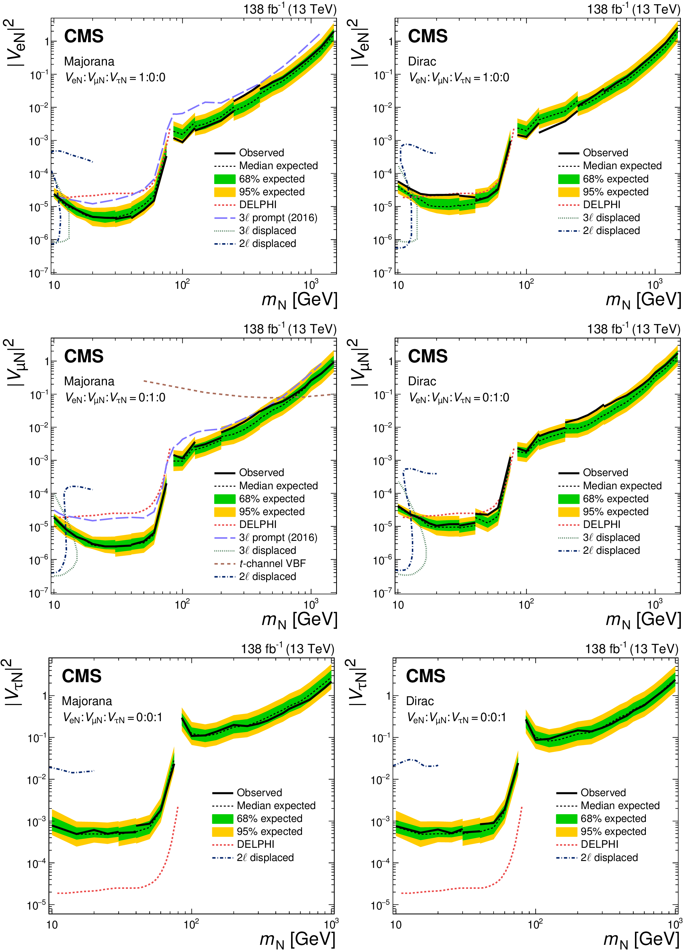
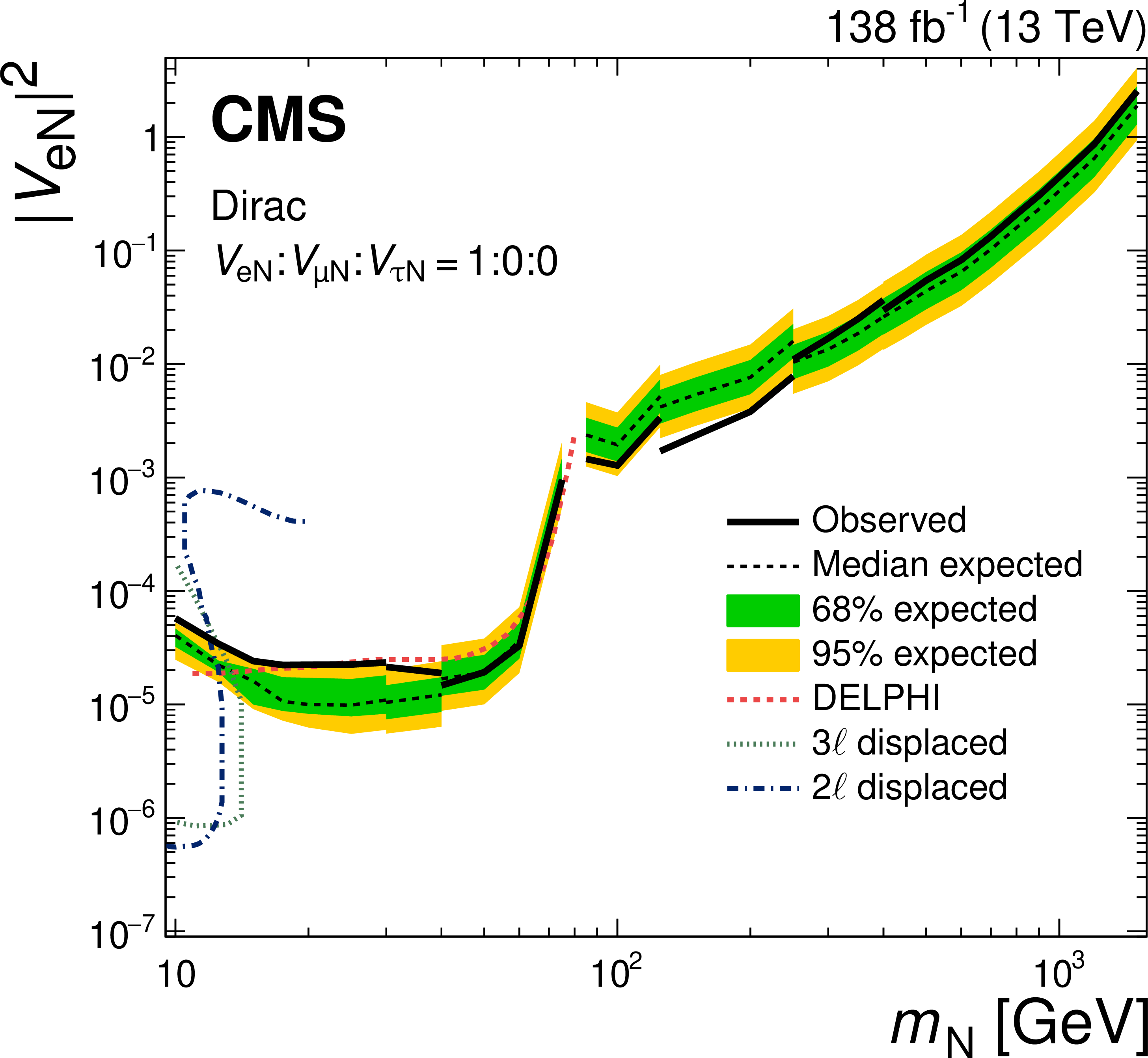
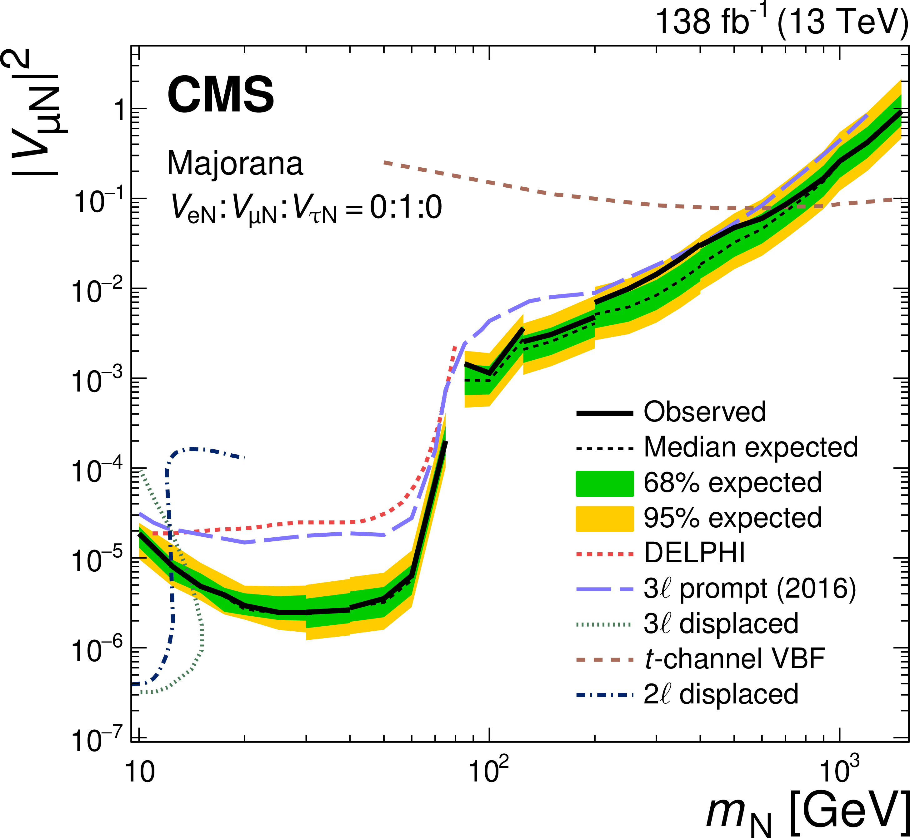
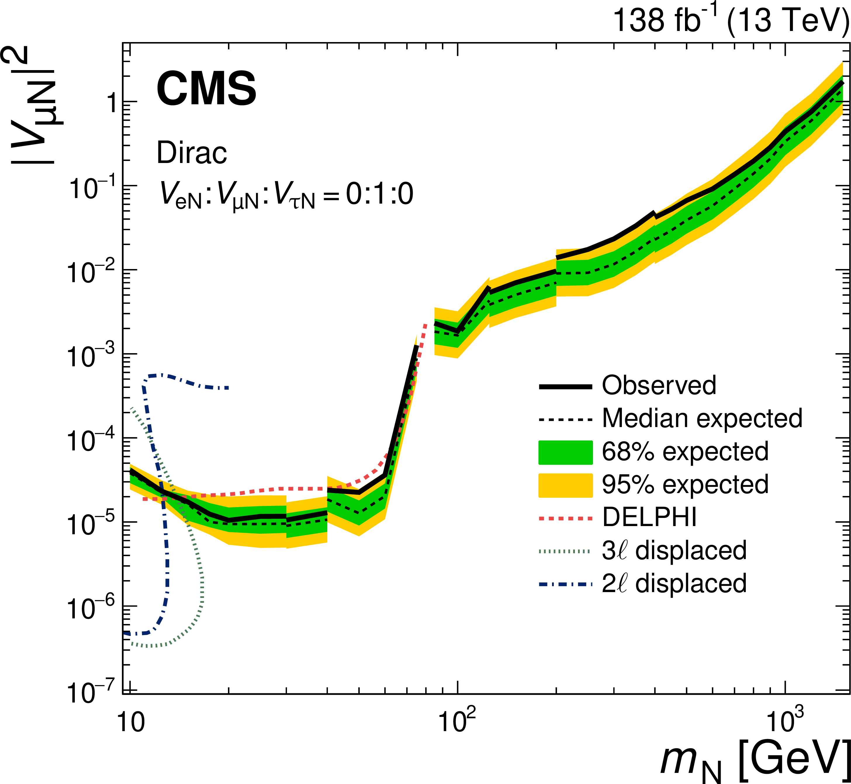
Figure 12:
The 95% CL limits on $ |V_{\mathrm{e}\mathrm{N}}|^2 $ (upper row), $ |V_{\mu\mathrm{N}}|^2 $ (middle row), and $ |V_{\tau\mathrm{N}}|^2 $ (lower row) as functions of $ m_{\mathrm{N}} $ for a Majorana (left) and Dirac (right) HNL. The area above the solid (dashed) black curve indicates the observed (expected) exclusion region. Previous results from the DELPHI Collaboration [134] are shown for reference. The previous CMS result ``3$\ell$ prompt (2016)'' [42] is shown to highlight the improvements achieved in our analysis, and the results ``3$\ell$ displaced'' [46], ``2$\ell$ displaced'' [48], and ``$ t $-channel VBF'' [135] are shown to highlight the complementarity to other search strategies. |

png pdf |
Figure 12-a:
The 95% CL limits on $ |V_{\mathrm{e}\mathrm{N}}|^2 $ (upper row), $ |V_{\mu\mathrm{N}}|^2 $ (middle row), and $ |V_{\tau\mathrm{N}}|^2 $ (lower row) as functions of $ m_{\mathrm{N}} $ for a Majorana (left) and Dirac (right) HNL. The area above the solid (dashed) black curve indicates the observed (expected) exclusion region. Previous results from the DELPHI Collaboration [134] are shown for reference. The previous CMS result ``3$\ell$ prompt (2016)'' [42] is shown to highlight the improvements achieved in our analysis, and the results ``3$\ell$ displaced'' [46], ``2$\ell$ displaced'' [48], and ``$ t $-channel VBF'' [135] are shown to highlight the complementarity to other search strategies. |
png pdf |
Figure 12-b:
The 95% CL limits on $ |V_{\mathrm{e}\mathrm{N}}|^2 $ (upper row), $ |V_{\mu\mathrm{N}}|^2 $ (middle row), and $ |V_{\tau\mathrm{N}}|^2 $ (lower row) as functions of $ m_{\mathrm{N}} $ for a Majorana (left) and Dirac (right) HNL. The area above the solid (dashed) black curve indicates the observed (expected) exclusion region. Previous results from the DELPHI Collaboration [134] are shown for reference. The previous CMS result ``3$\ell$ prompt (2016)'' [42] is shown to highlight the improvements achieved in our analysis, and the results ``3$\ell$ displaced'' [46], ``2$\ell$ displaced'' [48], and ``$ t $-channel VBF'' [135] are shown to highlight the complementarity to other search strategies. |
png pdf |
Figure 12-c:
The 95% CL limits on $ |V_{\mathrm{e}\mathrm{N}}|^2 $ (upper row), $ |V_{\mu\mathrm{N}}|^2 $ (middle row), and $ |V_{\tau\mathrm{N}}|^2 $ (lower row) as functions of $ m_{\mathrm{N}} $ for a Majorana (left) and Dirac (right) HNL. The area above the solid (dashed) black curve indicates the observed (expected) exclusion region. Previous results from the DELPHI Collaboration [134] are shown for reference. The previous CMS result ``3$\ell$ prompt (2016)'' [42] is shown to highlight the improvements achieved in our analysis, and the results ``3$\ell$ displaced'' [46], ``2$\ell$ displaced'' [48], and ``$ t $-channel VBF'' [135] are shown to highlight the complementarity to other search strategies. |
png pdf |
Figure 12-d:
The 95% CL limits on $ |V_{\mathrm{e}\mathrm{N}}|^2 $ (upper row), $ |V_{\mu\mathrm{N}}|^2 $ (middle row), and $ |V_{\tau\mathrm{N}}|^2 $ (lower row) as functions of $ m_{\mathrm{N}} $ for a Majorana (left) and Dirac (right) HNL. The area above the solid (dashed) black curve indicates the observed (expected) exclusion region. Previous results from the DELPHI Collaboration [134] are shown for reference. The previous CMS result ``3$\ell$ prompt (2016)'' [42] is shown to highlight the improvements achieved in our analysis, and the results ``3$\ell$ displaced'' [46], ``2$\ell$ displaced'' [48], and ``$ t $-channel VBF'' [135] are shown to highlight the complementarity to other search strategies. |
png pdf |
Figure 12-e:
The 95% CL limits on $ |V_{\mathrm{e}\mathrm{N}}|^2 $ (upper row), $ |V_{\mu\mathrm{N}}|^2 $ (middle row), and $ |V_{\tau\mathrm{N}}|^2 $ (lower row) as functions of $ m_{\mathrm{N}} $ for a Majorana (left) and Dirac (right) HNL. The area above the solid (dashed) black curve indicates the observed (expected) exclusion region. Previous results from the DELPHI Collaboration [134] are shown for reference. The previous CMS result ``3$\ell$ prompt (2016)'' [42] is shown to highlight the improvements achieved in our analysis, and the results ``3$\ell$ displaced'' [46], ``2$\ell$ displaced'' [48], and ``$ t $-channel VBF'' [135] are shown to highlight the complementarity to other search strategies. |
png pdf |
Figure 12-f:
The 95% CL limits on $ |V_{\mathrm{e}\mathrm{N}}|^2 $ (upper row), $ |V_{\mu\mathrm{N}}|^2 $ (middle row), and $ |V_{\tau\mathrm{N}}|^2 $ (lower row) as functions of $ m_{\mathrm{N}} $ for a Majorana (left) and Dirac (right) HNL. The area above the solid (dashed) black curve indicates the observed (expected) exclusion region. Previous results from the DELPHI Collaboration [134] are shown for reference. The previous CMS result ``3$\ell$ prompt (2016)'' [42] is shown to highlight the improvements achieved in our analysis, and the results ``3$\ell$ displaced'' [46], ``2$\ell$ displaced'' [48], and ``$ t $-channel VBF'' [135] are shown to highlight the complementarity to other search strategies. |
| Tables | |
png pdf |
Table 1:
Requirements on the light-lepton $ p_{\mathrm{T}} $ values in the online and offline selections. The first two columns give the numbers of electrons and muons in the event ($ N_{\mathrm{e}} $ and $ N_{\mu} $). The third column lists the $ p_{\mathrm{T}} $ thresholds on the reconstructed electrons and muons in the online trigger selection. The fourth column lists the offline event selection requirements applied in addition to the baseline requirements of $ \ptl1 > $ 15 GeV and $ \ptl{2,3} > $ 10 GeV. For the $ \mathrm{e}\mu $ trigger, the requirements are given for the highest and second-highest $ p_{\mathrm{T}} $ light lepton, referred to as $ \mathrm{l}_1 $ and $ \mathrm{l}_2 $. The values in parentheses give the thresholds applied in 2017 and 2018, where they are different from 2016. All events are required to pass the conditions of at least one of the rows. |
png pdf |
Table 2:
Definitions of the search regions (SRs) for events in the low-mass (upper part) and high-mass (lower part) selections. |
png pdf |
Table 3:
Relative impacts of the uncertainty sources in fits for six different fit models specified with $ m_{\mathrm{N}} $ value and coupling scenario, where the relative impact is defined as the ratio between the uncertainty from the respective source and the total uncertainty in the HNL signal strength. The symbol ``$ \text{--} $'' indicates that the corresponding uncertainty source is not applicable. |
png pdf |
Table 4:
Summary of the selections, categories, and distributions used in the maximum likelihood fits for the HNL signal points. |
| Summary |
| A search for heavy neutral leptons (HNLs) produced in proton-proton collisions at $ \sqrt{s} = $ 13 TeV has been presented. The data were collected with the CMS experiment at the LHC and correspond to an integrated luminosity of 138 fb$ ^{-1} $. Events with three charged leptons (electrons, muons, and hadronically decaying tau leptons) are selected, and dedicated identification criteria based on machine learning techniques are applied to reduce the contribution from nonprompt leptons not originating from the hard scattering process. Remaining standard model (SM) background contributions with nonprompt leptons are estimated from control samples in data, whereas other SM contributions that mostly stem from diboson production are estimated from Monte Carlo event simulations. A combination of categorization by kinematic properties and machine learning discriminants achieves optimal separation of the predicted signal and SM background contributions. No significant deviations from the SM predictions are observed. Exclusion limits at 95% confidence level are evaluated, assuming exclusive HNL couplings to a single generation of SM neutrinos in the mass range 10 GeV-1.5 TeV, for both Majorana and Dirac HNLs. These results exceed previous experimental constraints over large parts of the mass range. Constraints on tau neutrino couplings for HNL masses above the W boson mass are presented for the first time. |
| References | ||||
| 1 | Super-Kamiokande Collaboration | Evidence for oscillation of atmospheric neutrinos | PRL 81 (1998) 1562 | hep-ex/9807003 |
| 2 | SNO Collaboration | Direct evidence for neutrino flavor transformation from neutral-current interactions in the Sudbury Neutrino Observatory | PRL 89 (2002) 011301 | nucl-ex/0204008 |
| 3 | KamLAND Collaboration | First results from KamLAND: Evidence for reactor antineutrino disappearance | PRL 90 (2003) 021802 | hep-ex/0212021 |
| 4 | S. Bilenky | Neutrino oscillations: From a historical perspective to the present status | NPB 908 (2016) 2 | 1602.00170 |
| 5 | J. Formaggio, A. de Gouvêa, and R. Robertson | Direct measurements of neutrino mass | Phys. Rept. 914 (2021) 1 | 2102.00594 |
| 6 | KATRIN Collaboration | Direct neutrino-mass measurement with sub-electronvolt sensitivity | Nature Phys. 18 (2022) 160 | 2105.08533 |
| 7 | Planck Collaboration | Planck 2018 results. VI. cosmological parameters | Astron. Astrophys. 641 (2020) A6 | 1807.06209 |
| 8 | eBOSS Collaboration | Completed SDSS-IV extended baryon oscillation spectroscopic survey: Cosmological implications from two decades of spectroscopic surveys at the Apache Point Observatory | PRD 103 (2021) 083533 | 2007.08991 |
| 9 | Z. Sakr | A short review on the latest neutrinos mass and number constraints from cosmological observables | Universe 8 (2022) 284 | |
| 10 | P. Minkowski | $ {\mu\to\mathrm{e}\gamma} $ at a rate of one out of $ 10^9 $ muon decays? | PLB 67 (1977) 421 | |
| 11 | T. Yanagida | Horizontal gauge symmetry and masses of neutrinos | in Proc. Workshop on the Unified Theories and the Baryon Number in the Universe, Tsukuba, Japan, 1979 Conf. Proc. C 7902131 (1979) 95 |
|
| 12 | M. Gell-Mann, P. Ramond, and R. Slansky | Complex spinors and unified theories | in Supergravity, North Holland Publishing, 1979 | 1306.4669 |
| 13 | S. Glashow | The future of elementary particle physics | NATO Sci. Ser. B 61 (1980) 687 | |
| 14 | R. Mohapatra and G. Senjanović | Neutrino mass and spontaneous parity nonconservation | PRL 44 (1980) 912 | |
| 15 | J. Schechter and J. Valle | Neutrino masses in $ \mathrm{SU}(2)\otimes\mathrm{U}(1) $ theories | PRD 22 (1980) 2227 | |
| 16 | R. Shrock | General theory of weak leptonic and semileptonic decays. I. leptonic pseudoscalar meson decays, with associated tests for, and bounds on, neutrino masses and lepton mixing | PRD 24 (1981) 1232 | |
| 17 | Y. Cai, T. Han, T. Li, and R. Ruiz | Lepton number violation: Seesaw models and their collider tests | Front. Phys. 6 (2018) 40 | 1711.02180 |
| 18 | S. Dodelson and L. Widrow | Sterile neutrinos as dark matter | PRL 72 (1994) 17 | hep-ph/9303287 |
| 19 | A. Boyarsky et al. | Sterile neutrino dark matter | Prog. Part. Nucl. Phys. 104 (2019) 1 | 1807.07938 |
| 20 | M. Fukugita and T. Yanagida | Baryogenesis without grand unification | PLB 174 (1986) 45 | |
| 21 | E. Chun et al. | Probing leptogenesis | Int. J. Mod. Phys. A 33 (2018) 1842005 | 1711.02865 |
| 22 | M. Drewes, Y. Georis, and J. Klarić | Mapping the viable parameter space for testable leptogenesis | PRL 128 (2022) 051801 | 2106.16226 |
| 23 | J. Beacham et al. | Physics beyond colliders at CERN: Beyond the standard model working group report | JPG 47 (2020) 010501 | 1901.09966 |
| 24 | M. Drewes, J. Klarić , and J. López-Pavón | New benchmark models for heavy neutral lepton searches | EPJC 82 (2022) 1176 | 2207.02742 |
| 25 | F. del Aguila and J. Aguilar-Saavedra | Distinguishing seesaw models at LHC with multi-lepton signals | NPB 813 (2009) 22 | 0808.2468 |
| 26 | A. Atre, T. Han, S. Pascoli, and B. Zhang | The search for heavy Majorana neutrinos | JHEP 05 (2009) 030 | 0901.3589 |
| 27 | V. Tello et al. | Left-right symmetry: from LHC to neutrinoless double beta decay | PRL 106 (2011) 151801 | 1011.3522 |
| 28 | F. Deppisch, P. Bhupal Dev, and A. Pilaftsis | Neutrinos and collider physics | New J. Phys. 17 (2015) 075019 | 1502.06541 |
| 29 | S. Pascoli, R. Ruiz, and C. Weiland | Heavy neutrinos with dynamic jet vetoes: multilepton searches at $ \sqrt{s}= $ 14, 27, and 100 TeV | JHEP 06 (2019) 049 | 1812.08750 |
| 30 | A. Abdullahi et al. | The present and future status of heavy neutral leptons | JPG 50 (2023) 020501 | 2203.08039 |
| 31 | C. Antel et al. | Feebly interacting particles: FIPs 2022 workshop report | EPJC 83 (2023) 1122 | 2305.01715 |
| 32 | W.-Y. Keung and G. Senjanovic | Majorana neutrinos and the production of the right-handed charged gauge boson | PRL 50 (1983) 1427 | |
| 33 | S. Petcov | Possible signature for production of Majorana particles in $ \mathrm{e}^+ \mathrm{e}^- $ and $ {\mathrm{p}\overline{\mathrm{p}}} $ collisions | PLB 139 (1984) 421 | |
| 34 | A. Datta, M. Guchait, and A. Pilaftsis | Probing lepton number violation via Majorana neutrinos at hadron supercolliders | PRD 50 (1994) 3195 | hep-ph/9311257 |
| 35 | P. Bhupal Dev, A. Pilaftsis, and U.-k. Yang | New production mechanism for heavy neutrinos at the LHC | PRL 112 (2014) 081801 | 1308.2209 |
| 36 | D. Alva, T. Han, and R. Ruiz | Heavy Majorana neutrinos from $ {\mathrm{W}\gamma} $ fusion at hadron colliders | JHEP 02 (2015) 072 | 1411.7305 |
| 37 | C. Degrande, O. Mattelaer, R. Ruiz, and J. Turner | Fully-automated precision predictions for heavy neutrino production mechanisms at hadron colliders | PRD 94 (2016) 053002 | 1602.06957 |
| 38 | CMS Collaboration | Search for heavy Majorana neutrinos in $ {\mu^\pm\mu^\pm}+ $jets and $ {\mathrm{e}^\pm\mathrm{e}^\pm}+ $jets events in $ {\mathrm{p}\mathrm{p}} $ collisions at $ \sqrt{s}= $ 7 TeV | PLB 717 (2012) 109 | CMS-EXO-11-076 1207.6079 |
| 39 | CMS Collaboration | Search for heavy Majorana neutrinos in $ {\mu^\pm\mu^\pm}+ $jets events in proton-proton collisions at $ \sqrt{s}= $ 8 TeV | PLB 748 (2015) 144 | CMS-EXO-12-057 1501.05566 |
| 40 | ATLAS Collaboration | Search for heavy Majorana neutrinos with the ATLAS detector in $ {\mathrm{p}\mathrm{p}} $ collisions at $ \sqrt{s}= $ 8 TeV | JHEP 07 (2015) 162 | 1506.06020 |
| 41 | CMS Collaboration | Search for heavy Majorana neutrinos in $ {\mathrm{e}^\pm\mathrm{e}^\pm}+ $jets and $ {\mathrm{e}^\pm\mu^\pm}+ $jets events in proton-proton collisions at $ \sqrt{s}= $ 8 TeV | JHEP 04 (2016) 169 | CMS-EXO-14-014 1603.02248 |
| 42 | CMS Collaboration | Search for heavy neutral leptons in events with three charged leptons in proton-proton collisions at $ \sqrt{s}= $ 13 TeV | PRL 120 (2018) 221801 | CMS-EXO-17-012 1802.02965 |
| 43 | CMS Collaboration | Search for heavy Majorana neutrinos in same-sign dilepton channels in proton-proton collisions at $ \sqrt{s}= $ 13 TeV | JHEP 01 (2019) 122 | CMS-EXO-17-028 1806.10905 |
| 44 | ATLAS Collaboration | Search for heavy neutral leptons in decays of W bosons produced in 13 TeV $ {\mathrm{p}\mathrm{p}} $ collisions using prompt and displaced signatures with the ATLAS detector | JHEP 10 (2019) 265 | 1905.09787 |
| 45 | LHCb Collaboration | Search for heavy neutral leptons in $ {\mathrm{W^+}\to\mu^{+}\mu^\pm\,\text{jet}} $ decays | EPJC 81 (2021) 248 | 2011.05263 |
| 46 | CMS Collaboration | Search for long-lived heavy neutral leptons with displaced vertices in proton-proton collisions at $ \sqrt{s}= $ 13 TeV | JHEP 07 (2022) 081 | CMS-EXO-20-009 2201.05578 |
| 47 | ATLAS Collaboration | Search for heavy neutral leptons in decays of W bosons using a dilepton displaced vertex in $ \sqrt{s}= $ 13 TeV $ {\mathrm{p}\mathrm{p}} $ collisions with the ATLAS detector | PRL 131 (2023) 061803 | 2204.11988 |
| 48 | CMS Collaboration | Search for long-lived heavy neutral leptons with lepton flavour conserving or violating decays to a jet and a charged lepton | Submitted to JHEP, 2023 | CMS-EXO-21-013 2312.07484 |
| 49 | A. Abada, N. Bernal, M. Losada, and X. Marcano | Inclusive displaced vertex searches for heavy neutral leptons at the LHC | JHEP 01 (2019) 093 | 1807.10024 |
| 50 | J.-L. Tastet, O. Ruchayskiy, and I. Timiryasov | Reinterpreting the ATLAS bounds on heavy neutral leptons in a realistic neutrino oscillation model | JHEP 12 (2021) 182 | 2107.12980 |
| 51 | CMS Collaboration | HEPData record for this analysis | link | |
| 52 | T. Asaka, S. Blanchet, and M. Shaposhnikov | The \PGnMSM, dark matter and neutrino masses | PLB 631 (2005) 151 | hep-ph/0503065 |
| 53 | CMS Collaboration | The CMS experiment at the CERN LHC | JINST 3 (2008) S08004 | |
| 54 | CMS Collaboration | Development of the CMS detector for the CERN LHC Run 3 | Accepted by JINST, 2023 | CMS-PRF-21-001 2309.05466 |
| 55 | CMS Collaboration | Performance of the CMS Level-1 trigger in proton-proton collisions at $ \sqrt{s}= $ 13 TeV | JINST 15 (2020) P10017 | CMS-TRG-17-001 2006.10165 |
| 56 | CMS Collaboration | The CMS trigger system | JINST 12 (2017) P01020 | CMS-TRG-12-001 1609.02366 |
| 57 | CMS Collaboration | Particle-flow reconstruction and global event description with the CMS detector | JINST 12 (2017) P10003 | CMS-PRF-14-001 1706.04965 |
| 58 | CMS Collaboration | Technical proposal for the Phase-II upgrade of the Compact Muon Solenoid | CMS Technical Proposal CERN-LHCC-2015-010, CMS-TDR-15-02, 2015 CDS |
|
| 59 | M. Cacciari, G. P. Salam, and G. Soyez | The anti-$ k_{\mathrm{T}} $ jet clustering algorithm | JHEP 04 (2008) 063 | 0802.1189 |
| 60 | M. Cacciari, G. P. Salam, and G. Soyez | FASTJET user manual | EPJC 72 (2012) 1896 | 1111.6097 |
| 61 | CMS Collaboration | Jet energy scale and resolution in the CMS experiment in $ {\mathrm{p}\mathrm{p}} $ collisions at 8 TeV | JINST 12 (2017) P02014 | CMS-JME-13-004 1607.03663 |
| 62 | CMS Collaboration | Jet algorithms performance in 13 TeV data | CMS Physics Analysis Summary, 2017 CMS-PAS-JME-16-003 |
CMS-PAS-JME-16-003 |
| 63 | CMS Collaboration | Performance of missing transverse momentum reconstruction in proton-proton collisions at $ \sqrt{s}= $ 13 TeV using the CMS detector | JINST 14 (2019) P07004 | CMS-JME-17-001 1903.06078 |
| 64 | CMS Collaboration | Identification of heavy-flavour jets with the CMS detector in $ {\mathrm{p}\mathrm{p}} $ collisions at 13 TeV | JINST 13 (2018) P05011 | CMS-BTV-16-002 1712.07158 |
| 65 | E. Bols et al. | Jet flavour classification using DeepJet | JINST 15 (2020) P12012 | 2008.10519 |
| 66 | CMS Collaboration | Performance summary of AK4 jet b tagging with data from proton-proton collisions at 13 TeV with the CMS detector | CMS Detector Performance Note CMS-DP-2023-005, 2023 CDS |
|
| 67 | GEANT4 Collaboration | GEANT 4---a simulation toolkit | NIM A 506 (2003) 250 | |
| 68 | CMS Collaboration | Pileup mitigation at CMS in 13 TeV data | JINST 15 (2020) P09018 | CMS-JME-18-001 2003.00503 |
| 69 | J. Alwall et al. | The automated computation of tree-level and next-to-leading order differential cross sections, and their matching to parton shower simulations | JHEP 07 (2014) 079 | 1405.0301 |
| 70 | P. Artoisenet, R. Frederix, O. Mattelaer, and R. Rietkerk | Automatic spin-entangled decays of heavy resonances in Monte Carlo simulations | JHEP 03 (2013) 015 | 1212.3460 |
| 71 | NNPDF Collaboration | Parton distributions from high-precision collider data | EPJC 77 (2017) 663 | 1706.00428 |
| 72 | A. Manohar, P. Nason, G. P. Salam, and G. Zanderighi | How bright is the proton? A precise determination of the photon parton distribution function | PRL 117 (2016) 242002 | 1607.04266 |
| 73 | A. V. Manohar, P. Nason, G. P. Salam, and G. Zanderighi | The photon content of the proton | JHEP 12 (2017) 046 | 1708.01256 |
| 74 | NNPDF Collaboration | Illuminating the photon content of the proton within a global PDF analysis | SciPost Phys. 5 (2018) 008 | 1712.07053 |
| 75 | K. Bondarenko, A. Boyarsky, D. Gorbunov, and O. Ruchayskiy | Phenomenology of GeVns-scale heavy neutral leptons | JHEP 11 (2018) 032 | 1805.08567 |
| 76 | P. Nason | A new method for combining NLO QCD with shower Monte Carlo algorithms | JHEP 11 (2004) 040 | hep-ph/0409146 |
| 77 | S. Frixione, G. Ridolfi, and P. Nason | A positive-weight next-to-leading-order Monte Carlo for heavy flavour hadroproduction | JHEP 09 (2007) 126 | 0707.3088 |
| 78 | S. Frixione, P. Nason, and C. Oleari | Matching NLO QCD computations with parton shower simulations: the POWHEG method | JHEP 11 (2007) 070 | 0709.2092 |
| 79 | S. Alioli, P. Nason, C. Oleari, and E. Re | NLO single-top production matched with shower in POWHEG: $ s $- and $ t $-channel contributions | JHEP 09 (2009) 111 | 0907.4076 |
| 80 | P. Nason and C. Oleari | NLO Higgs boson production via vector-boson fusion matched with shower in POWHEG | JHEP 02 (2010) 037 | 0911.5299 |
| 81 | S. Alioli, P. Nason, C. Oleari, and E. Re | A general framework for implementing NLO calculations in shower Monte Carlo programs: the POWHEG \textscbox | JHEP 06 (2010) 043 | 1002.2581 |
| 82 | E. Re | Single-top $ {\mathrm{W}\mathrm{t}} $-channel production matched with parton showers using the POWHEG method | EPJC 71 (2011) 1547 | 1009.2450 |
| 83 | E. Bagnaschi, G. Degrassi, P. Slavich, and A. Vicini | Higgs production via gluon fusion in the POWHEG approach in the SM and in the MSSM | JHEP 02 (2012) 088 | 1111.2854 |
| 84 | P. Nason and G. Zanderighi | $ {\mathrm{W^+}\mathrm{W^-}} $, $ {\mathrm{W}\mathrm{Z}} $ and $ {\mathrm{Z}\mathrm{Z}} $ production in the POWHEG -\textscbox-v2 | EPJC 74 (2014) 2702 | 1311.1365 |
| 85 | J. M. Campbell and R. K. Ellis | An update on vector boson pair production at hadron colliders | PRD 60 (1999) 113006 | hep-ph/9905386 |
| 86 | J. M. Campbell, R. K. Ellis, and C. Williams | Vector boson pair production at the LHC | JHEP 07 (2011) 018 | 1105.0020 |
| 87 | J. M. Campbell, R. K. Ellis, and W. T. Giele | A multi-threaded version of MCFM | EPJC 75 (2015) 246 | 1503.06182 |
| 88 | T. Sjöstrand et al. | An introduction to PYTHIA8.2 | Comput. Phys. Commun. 191 (2015) 159 | 1410.3012 |
| 89 | CMS Collaboration | Extraction and validation of a new set of CMS PYTHIA8 tunes from underlying-event measurements | EPJC 80 (2020) 4 | CMS-GEN-17-001 1903.12179 |
| 90 | J. Alwall et al. | Comparative study of various algorithms for the merging of parton showers and matrix elements in hadronic collisions | EPJC 53 (2008) 473 | 0706.2569 |
| 91 | R. Frederix and S. Frixione | Merging meets matching in MC@NLO | JHEP 12 (2012) 061 | 1209.6215 |
| 92 | S. Bolognesi et al. | On the spin and parity of a single-produced resonance at the LHC | PRD 86 (2012) 095031 | 1208.4018 |
| 93 | CMS Collaboration | Electron and photon reconstruction and identification with the CMS experiment at the CERN LHC | JINST 16 (2021) P05014 | CMS-EGM-17-001 2012.06888 |
| 94 | CMS Collaboration | ECAL 2016 refined calibration and Run2 summary plots | CMS Detector Performance Note CMS-DP-2020-021, 2020 CDS |
|
| 95 | CMS Collaboration | Performance of the CMS muon detector and muon reconstruction with proton-proton collisions at $ \sqrt{s}= $ 13 TeV | JINST 13 (2018) P06015 | CMS-MUO-16-001 1804.04528 |
| 96 | K. Rehermann and B. Tweedie | Efficient identification of boosted semileptonic top quarks at the LHC | JHEP 03 (2011) 059 | 1007.2221 |
| 97 | CMS Collaboration | Observation of four top quark production in proton-proton collisions at $ \sqrt{s}= $ 13 TeV | PLB 847 (2023) 138290 | CMS-TOP-22-013 2305.13439 |
| 98 | CMS Collaboration | Evidence for associated production of a Higgs boson with a top quark pair in final states with electrons, muons, and hadronically decaying $ \tau $ leptons at $ \sqrt{s}= $ 13 TeV | JHEP 08 (2018) 066 | CMS-HIG-17-018 1803.05485 |
| 99 | CMS Collaboration | Observation of single top quark production in association with a Z boson in proton-proton collisions at $ \sqrt{s}= $ 13 TeV | PRL 122 (2019) 132003 | CMS-TOP-18-008 1812.05900 |
| 100 | CMS Collaboration | Measurement of the Higgs boson production rate in association with top quarks in final states with electrons, muons, and hadronically decaying tau leptons at $ \sqrt{s}= $ 13 TeV | EPJC 81 (2021) 378 | CMS-HIG-19-008 2011.03652 |
| 101 | CMS Collaboration | Search for electroweak production of charginos and neutralinos in proton-proton collisions at $ \sqrt{s}= $ 13 TeV | JHEP 04 (2022) 147 | CMS-SUS-19-012 2106.14246 |
| 102 | CMS Collaboration | Measurements of the electroweak diboson production cross sections in proton-proton collisions at $ \sqrt{s}= $ 5.02 TeV using leptonic decays | PRL 127 (2021) 191801 | CMS-SMP-20-012 2107.01137 |
| 103 | CMS Collaboration | Inclusive and differential cross section measurements of single top quark production in association with a Z boson in proton-proton collisions at $ \sqrt{s}= $ 13 TeV | JHEP 02 (2022) 107 | CMS-TOP-20-010 2111.02860 |
| 104 | CMS Collaboration | Muon identification using multivariate techniques in the CMS experiment in proton-proton collisions at $ \sqrt{s}= $ 13 TeV | Accepted by JINST, 2023 | CMS-MUO-22-001 2310.03844 |
| 105 | CMS Collaboration | Performance of reconstruction and identification of $ \tau $ leptons decaying to hadrons and $ \nu_{\!\tau} $ in $ {\mathrm{p}\mathrm{p}} $ collisions at $ \sqrt{s}= $ 13 TeV | JINST 13 (2018) P10005 | CMS-TAU-16-003 1809.02816 |
| 106 | CMS Collaboration | Identification of hadronic tau lepton decays using a deep neural network | JINST 17 (2022) P07023 | CMS-TAU-20-001 2201.08458 |
| 107 | Particle Data Group , R. L. Workman et al. | Review of particle physics | Prog. Theor. Exp. Phys. 2022 (2022) 083C01 | |
| 108 | CMS Collaboration | Performance of electron reconstruction and selection with the CMS detector in proton-proton collisions at $ \sqrt{s}= $ 8 TeV | JINST 10 (2015) P06005 | CMS-EGM-13-001 1502.02701 |
| 109 | CMS Collaboration | Performance of CMS muon reconstruction in cosmic-ray events | JINST 5 (2010) T03022 | CMS-CFT-09-014 0911.4994 |
| 110 | CMS Collaboration | Performance of the reconstruction and identification of high-momentum muons in proton-proton collisions at $ \sqrt{s}= $ 13 TeV | JINST 15 (2020) P02027 | CMS-MUO-17-001 1912.03516 |
| 111 | H. Voss, A. Höcker, J. Stelzer, and F. Tegenfeldt | TMVA, the toolkit for multivariate data analysis with ROOT | in Proc. 11th Int. Workshop on Advanced Computing and Analysis Techniques in Phys. Research (ACAT ): Amsterdam, The Netherlands, 2017 [PoS (ACAT2017) 040] |
physics/0703039 |
| 112 | CMS Collaboration | Search for new physics in same-sign dilepton events in proton-proton collisions at $ \sqrt{s}= $ 13 TeV | EPJC 76 (2016) 439 | CMS-SUS-15-008 1605.03171 |
| 113 | CMS Collaboration | Measurement of the cross section of top quark-antiquark pair production in association with a W boson in proton-proton collisions at $ \sqrt{s}= $ 13 TeV | JHEP 07 (2023) 219 | CMS-TOP-21-011 2208.06485 |
| 114 | CMS Collaboration | Precision luminosity measurement in proton-proton collisions at $ \sqrt{s}= $ 13 TeV in 2015 and 2016 at CMS | EPJC 81 (2021) 800 | CMS-LUM-17-003 2104.01927 |
| 115 | CMS Collaboration | CMS luminosity measurement for the 2017 data-taking period at $ \sqrt{s}= $ 13 TeV | CMS Physics Analysis Summary, 2018 CMS-PAS-LUM-17-004 |
CMS-PAS-LUM-17-004 |
| 116 | CMS Collaboration | CMS luminosity measurement for the 2018 data-taking period at $ \sqrt{s}= $ 13 TeV | CMS Physics Analysis Summary, 2019 CMS-PAS-LUM-18-002 |
CMS-PAS-LUM-18-002 |
| 117 | CMS Collaboration | Measurements of inclusive W and Z cross sections in $ {\mathrm{p}\mathrm{p}} $ collisions at $ \sqrt{s}= $ 7 TeV | JHEP 01 (2011) 080 | CMS-EWK-10-002 1012.2466 |
| 118 | A. Lazopoulos, K. Melnikov, and F. Petriello | QCD corrections to tri-boson production | PRD 76 (2007) 014001 | hep-ph/0703273 |
| 119 | T. Binoth, G. Ossola, C. G. Papadopoulos, and R. Pittau | NLO QCD corrections to tri-boson production | JHEP 06 (2008) 082 | 0804.0350 |
| 120 | V. Hankele and D. Zeppenfeld | QCD corrections to hadronic $ {\mathrm{W}\mathrm{W}\mathrm{Z}} $ production with leptonic decays | PLB 661 (2008) 103 | 0712.3544 |
| 121 | F. Campanario et al. | QCD corrections to charged triple vector boson production with leptonic decay | PRD 78 (2008) 094012 | 0809.0790 |
| 122 | S. Dittmaier, A. Huss, and G. Knippen | Next-to-leading-order QCD and electroweak corrections to $ {\mathrm{W}\mathrm{W}\mathrm{W}} $ production at proton-proton colliders | JHEP 09 (2017) 034 | 1705.03722 |
| 123 | CMS Collaboration | A portrait of the Higgs boson by the CMS experiment ten years after the discovery | Nature 607 (2022) 60 | CMS-HIG-22-001 2207.00043 |
| 124 | K. Melnikov and F. Petriello | Electroweak gauge boson production at hadron colliders through $ \mathcal{O}({\alpha_\mathrm{S}^2}) $ | PRD 74 (2006) 114017 | hep-ph/0609070 |
| 125 | R. Gavin, Y. Li, F. Petriello, and S. Quackenbush | FEWZ 2.0: A code for hadronic Z production at next-to-next-to-leading order | Comput. Phys. Commun. 182 (2011) 2388 | 1011.3540 |
| 126 | R. Gavin, Y. Li, F. Petriello, and S. Quackenbush | W physics at the LHC with FEWZ 2.1 | Comput. Phys. Commun. 184 (2013) 208 | 1201.5896 |
| 127 | Y. Li and F. Petriello | Combining QCD and electroweak corrections to dilepton production in FEWZ | PRD 86 (2012) 094034 | 1208.5967 |
| 128 | ATLAS and CMS Collaborations, and LHC Higgs Combination Group | Procedure for the LHC Higgs boson search combination in Summer 2011 | Technical Report CMS-NOTE-2011-005, ATL-PHYS-PUB-2011-11, 2011 | |
| 129 | R. Barlow and C. Beeston | Fitting using finite Monte Carlo samples | Comput. Phys. Commun. 77 (1993) 219 | |
| 130 | J. S. Conway | Incorporating nuisance parameters in likelihoods for multisource spectra | in Proc. 2011 Workshop on Statistical Issues Related to Discovery Claims in Search Experiments and Unfolding (PHYSTAT ): Geneva, Switzerland, 2011 link |
1103.0354 |
| 131 | T. Junk | Confidence level computation for combining searches with small statistics | NIM A 434 (1999) 435 | hep-ex/9902006 |
| 132 | A. L. Read | Presentation of search results: The $ \text{CL}_\text{s} $ technique | JPG 28 (2002) 2693 | |
| 133 | G. Cowan, K. Cranmer, E. Gross, and O. Vitells | Asymptotic formulae for likelihood-based tests of new physics | EPJC 71 (2011) 1554 | 1007.1727 |
| 134 | DELPHI Collaboration | Search for neutral heavy leptons produced in Z decays | Z. Phys. C 74 (1997) 57 | |
| 135 | CMS Collaboration | Probing heavy Majorana neutrinos and the Weinberg operator through vector boson fusion processes in proton-proton collisions at $ \sqrt{s}= $ 13 TeV | PRL 131 (2023) 011803 | CMS-EXO-21-003 2206.08956 |
| 136 | BaBar Collaboration | Search for heavy neutral leptons using tau lepton decays at BaBaR | PRD 107 (2023) 052009 | 2207.09575 |
|
|
Compact Muon Solenoid LHC, CERN |
|

|

|

|

|

|