

Compact Muon Solenoid
LHC, CERN
| CMS-SUS-21-002 ; CERN-EP-2022-031 | ||
| Search for electroweak production of charginos and neutralinos at $\sqrt{s} = $ 13 TeV in final states containing hadronic decays of WW, WZ, or WH and missing transverse momentum | ||
| CMS Collaboration | ||
| 19 May 2022 | ||
| Phys. Lett. B 842 (2023) 137460 | ||
| Abstract: This Letter presents a search for direct production of charginos and neutralinos via electroweak interactions. The results are based on data from proton-proton collisions at a center-of-mass energy of 13 TeV collected with the CMS detector at the LHC, corresponding to an integrated luminosity of 137 fb$^{-1}$. The search considers final states with large missing transverse momentum and pairs of hadronically decaying bosons WW, WZ, and WH, where H is the Higgs boson. These bosons are identified using novel algorithms. No significant excess of events is observed relative to the expectations from the standard model. Limits at the 95% confidence level are placed on the cross section for production of mass-degenerate wino-like supersymmetric particles $\tilde{\chi}^{\pm}_1$ and $\tilde{\chi}^{0}_2$, and mass-degenerate higgsino-like supersymmetric particles $\tilde{\chi}^{\pm}_1$, $\tilde{\chi}^{0}_2$, and $\tilde{\chi}^{0}_3$. In the limit of a nearly-massless lightest supersymmetric particle $\tilde{\chi}^0_1$, wino-like particles with masses up to 870 and 960 GeV are excluded in the cases of $\tilde{\chi}^{0}_2\to\mathrm{Z}\tilde{\chi}^0_1$ and $\tilde{\chi}^{0}_2\to\mathrm{H}\tilde{\chi}^0_1$, respectively, and higgsino-like particles are excluded between 300 and 650 GeV. | ||
| Links: e-print arXiv:2205.09597 [hep-ex] (PDF) ; CDS record ; inSPIRE record ; HepData record ; CADI line (restricted) ; | ||
| Figures & Tables | Summary | Additional Figures & Tables | References | CMS Publications |
|---|
| Figures | |
png pdf |
Figure 1:
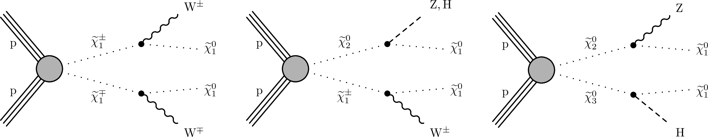
Diagram for the production of $ \tilde\chi_1^\pm \tilde\chi_1^\mp $ with the $ \tilde\chi_1^\pm $ decaying to a W boson and $ \tilde\chi_1^0 $ (left). In the $ \tilde\chi_1^\pm\tilde\chi_2^0 $ production diagram (middle) the $ \tilde\chi_1^\pm $ decays to a W boson and the $ \tilde\chi_2^0 $ decays to either a Z boson or a Higgs boson and $ \tilde\chi_1^0 $. In the case of $ \tilde\chi_2^0\tilde\chi_3^0 $ prduction (right) the $ \tilde\chi_2^0 $ and $ \tilde\chi_3^0 $ decay to a Z boson and Higgs boson, respectively, along with a $ \tilde\chi_1^0 $ each. |
png pdf |
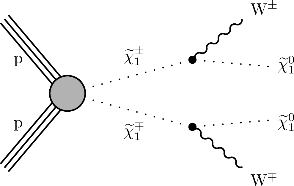
Figure 1-a:
Diagram for the production of $ \tilde\chi_1^\pm \tilde\chi_1^\mp $ with the $ \tilde\chi_1^\pm $ decaying to a W boson and $ \tilde\chi_1^0 $. |
png pdf |
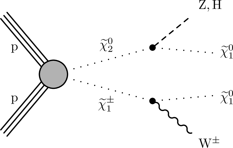
Figure 1-b:
In the $ \tilde\chi_1^\pm\tilde\chi_2^0 $ production diagram the $ \tilde\chi_1^\pm $ decays to a W boson and the $ \tilde\chi_2^0 $ decays to either a Z boson or a Higgs boson and $ \tilde\chi_1^0 $. |

png pdf |
Figure 1-c:
In the case of $ \tilde\chi_2^0\tilde\chi_3^0 $ production the $ \tilde\chi_2^0 $ and $ \tilde\chi_3^0 $ decay to a Z boson and Higgs boson, respectively, along with a $ \tilde\chi_1^0 $ each. |
png pdf |
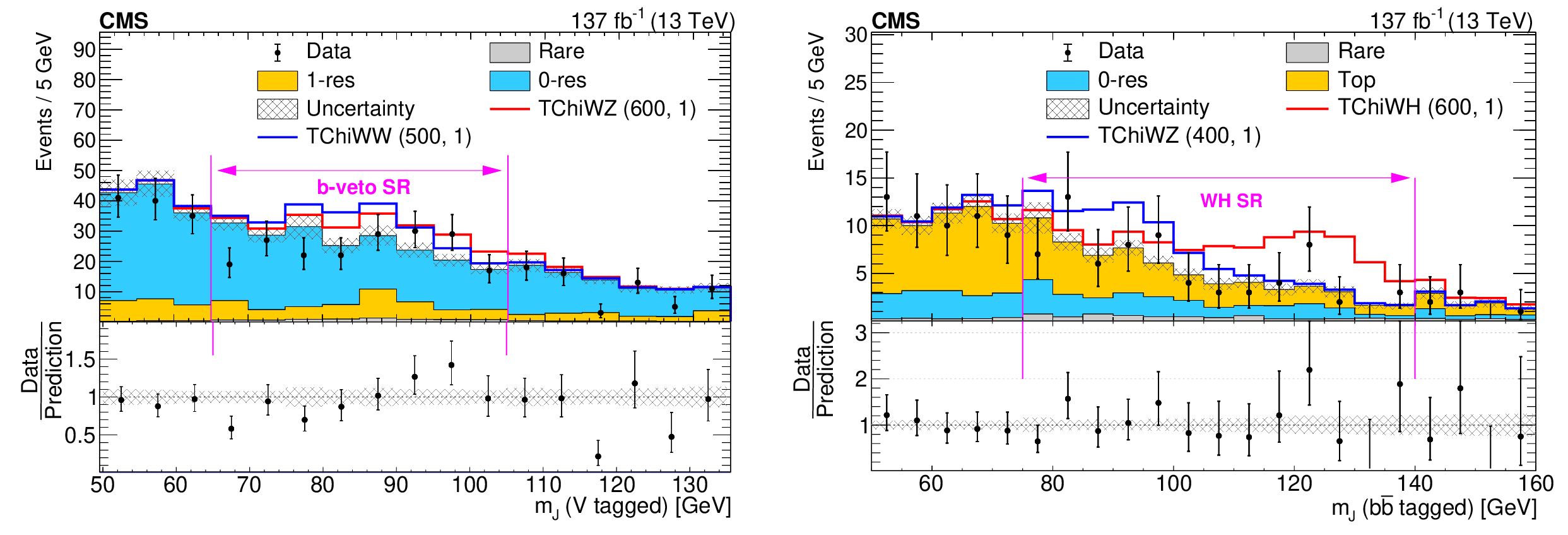
Figure 2:
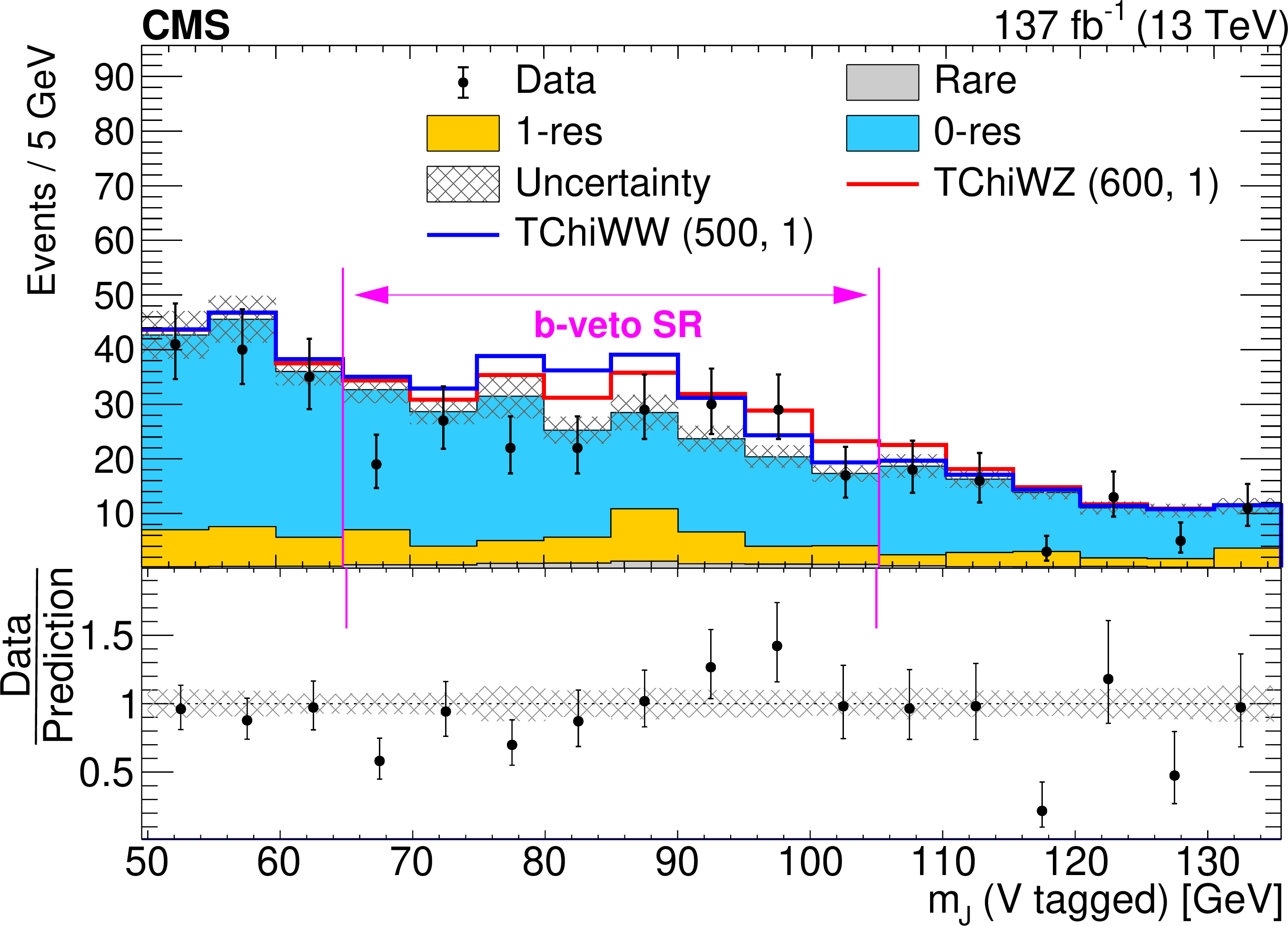
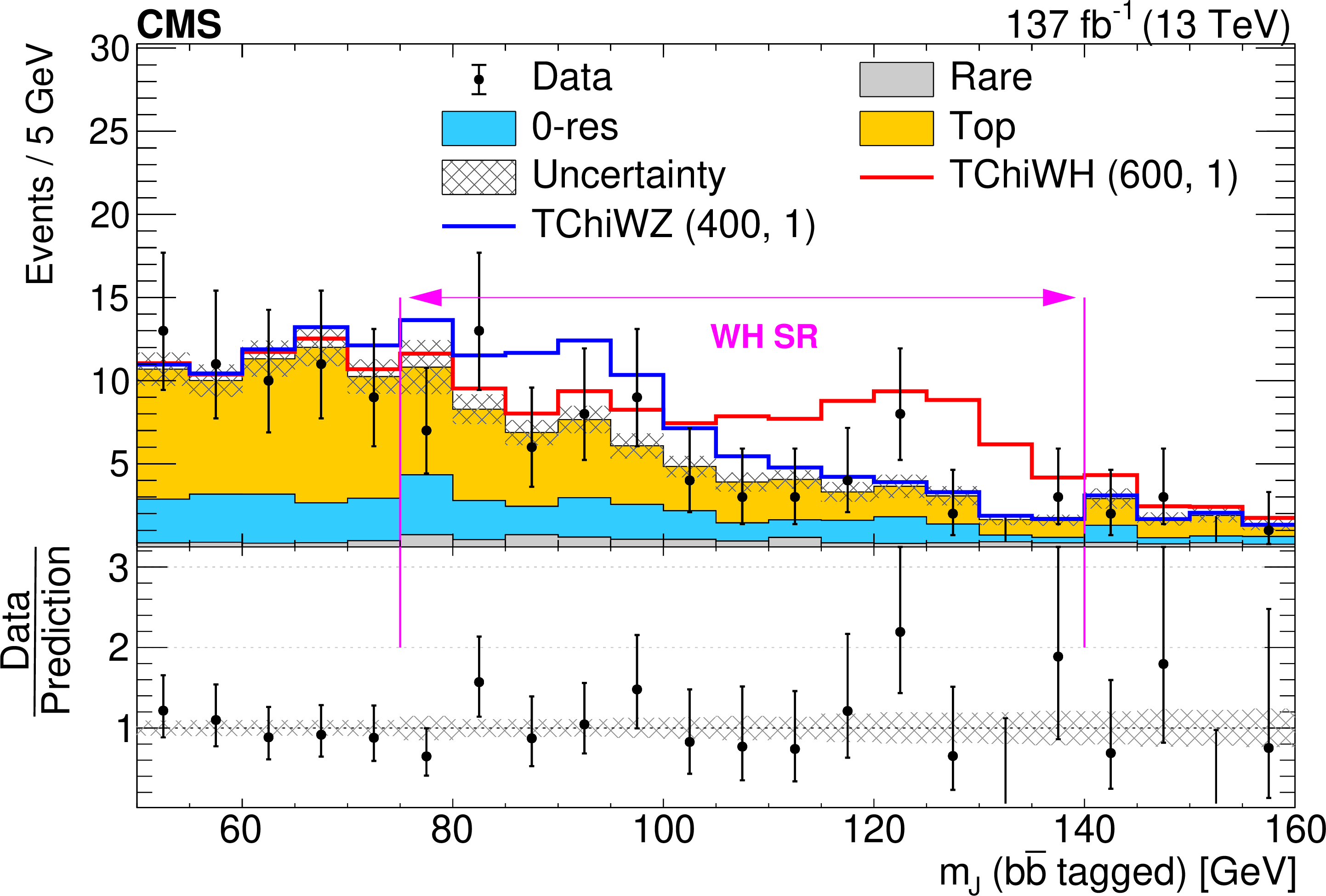
Distributions of the jet mass for V-tagged AK8 jets in the b-veto SR (left) and ${\mathrm{b} \mathrm{\bar{b}}} $-tagged AK8 jets in the WH SR (right). The jet mass requirements for the V and ${\mathrm{b} \mathrm{\bar{b}}}$ taggers have been loosened in these figures. The filled histograms show the SM background simulation, scaled such that the yield within the SR matches the total SM background predictions. The open histograms show the sum of the scaled SM background simulations and of the expectations for selected signal models, which are denoted in the legend by the name of the model followed by the assumed masses of the NLSP and LSP in GeV. The observed event yields are indicated by black markers. The hatched gray bands correspond to the statistical uncertainties in the SM predictions, but no systematic uncertainties are included. |
png pdf |
Figure 2-a:
Distribution of the jet mass for V-tagged AK8 jets in the b-veto SR. The jet mass requirements have been loosened in the figure. The filled histograms show the SM background simulation, scaled such that the yield within the SR matches the total SM background predictions. The open histograms show the sum of the scaled SM background simulations and of the expectations for selected signal models, which are denoted in the legend by the name of the model followed by the assumed masses of the NLSP and LSP in GeV. The observed event yields are indicated by black markers. The hatched gray bands correspond to the statistical uncertainties in the SM predictions, but no systematic uncertainties are included. |
png pdf |
Figure 2-b:
Distribution of the jet mass for ${\mathrm{b} \mathrm{\bar{b}}} $-tagged AK8 jets in the WH SR. The jet mass requirements have been loosened in the figure. The filled histograms show the SM background simulation, scaled such that the yield within the SR matches the total SM background predictions. The open histograms show the sum of the scaled SM background simulations and of the expectations for selected signal models, which are denoted in the legend by the name of the model followed by the assumed masses of the NLSP and LSP in GeV. The observed event yields are indicated by black markers. The hatched gray bands correspond to the statistical uncertainties in the SM predictions, but no systematic uncertainties are included. |
png pdf |
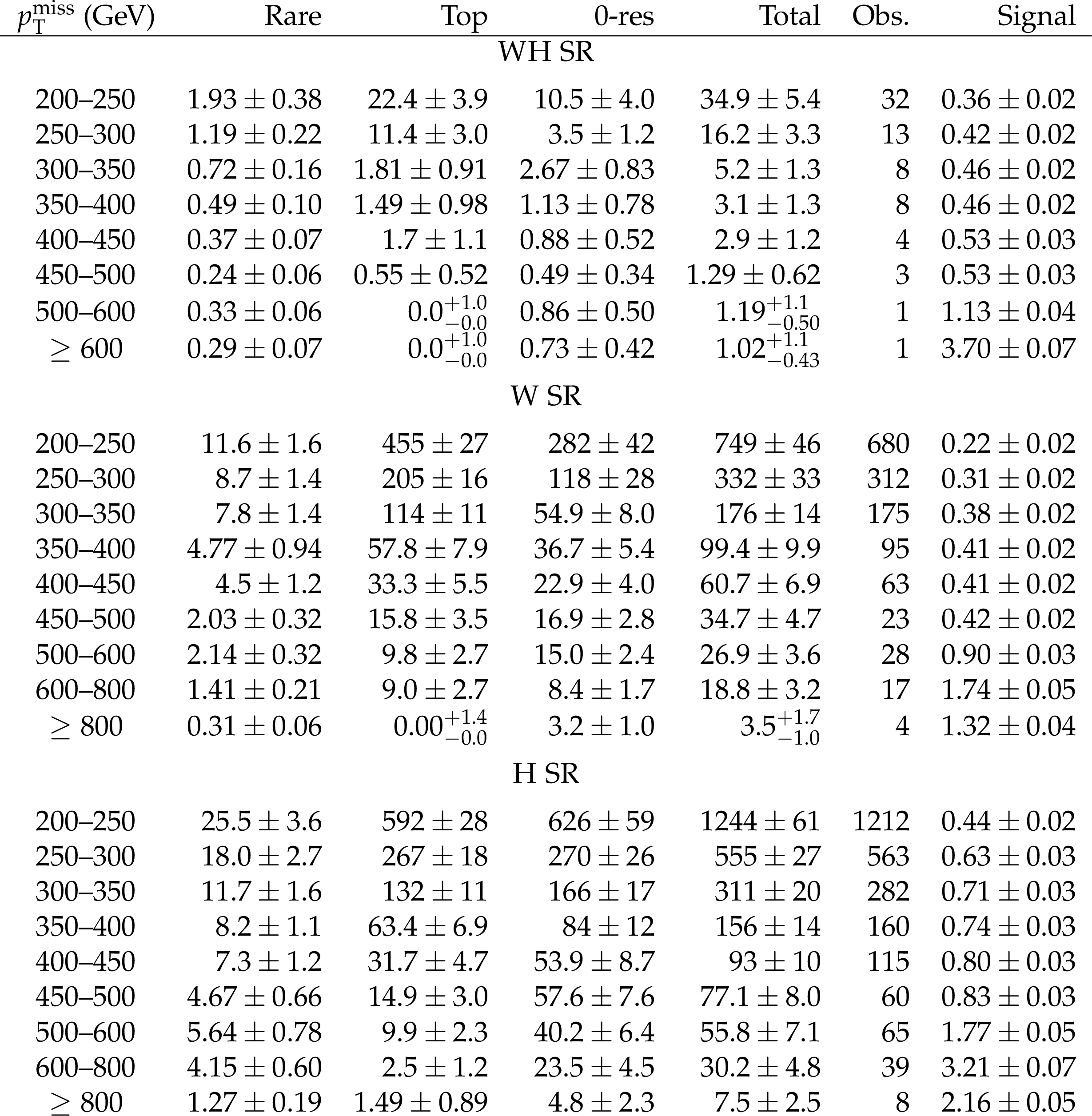
Figure 3:
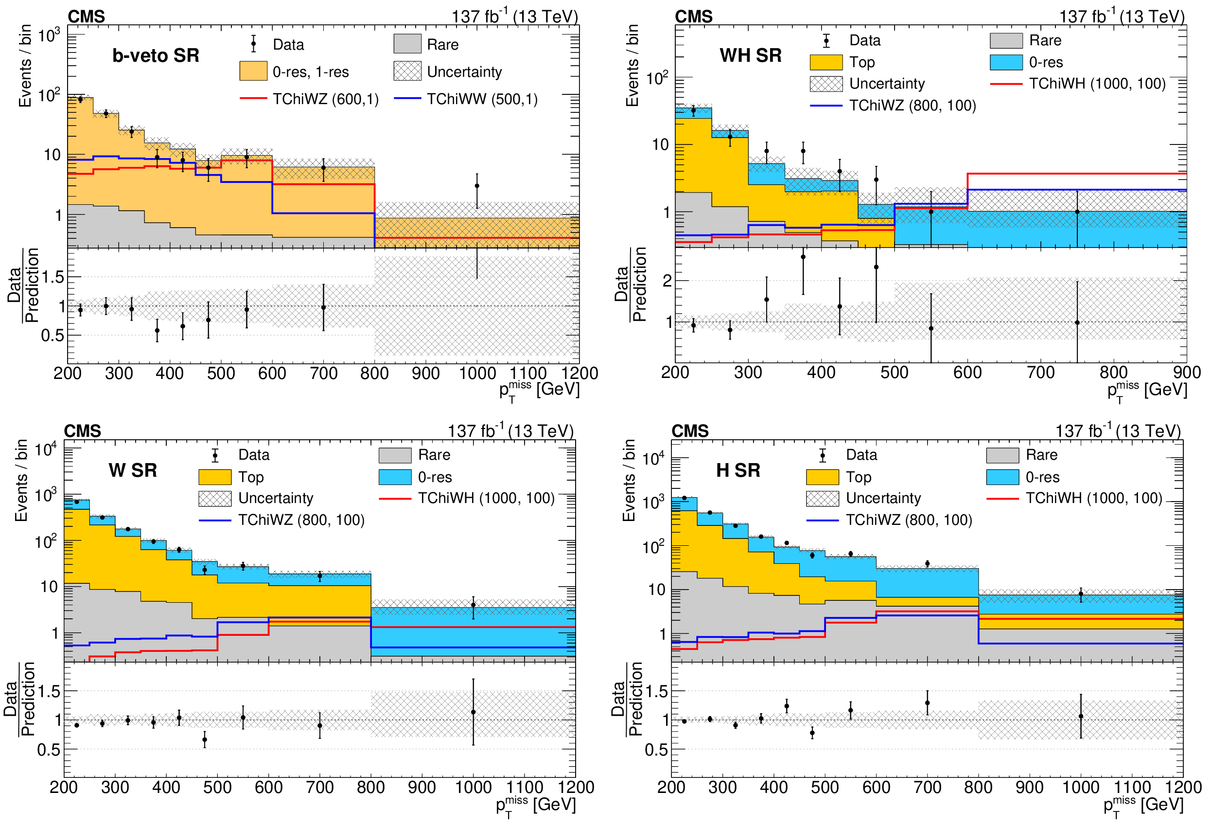
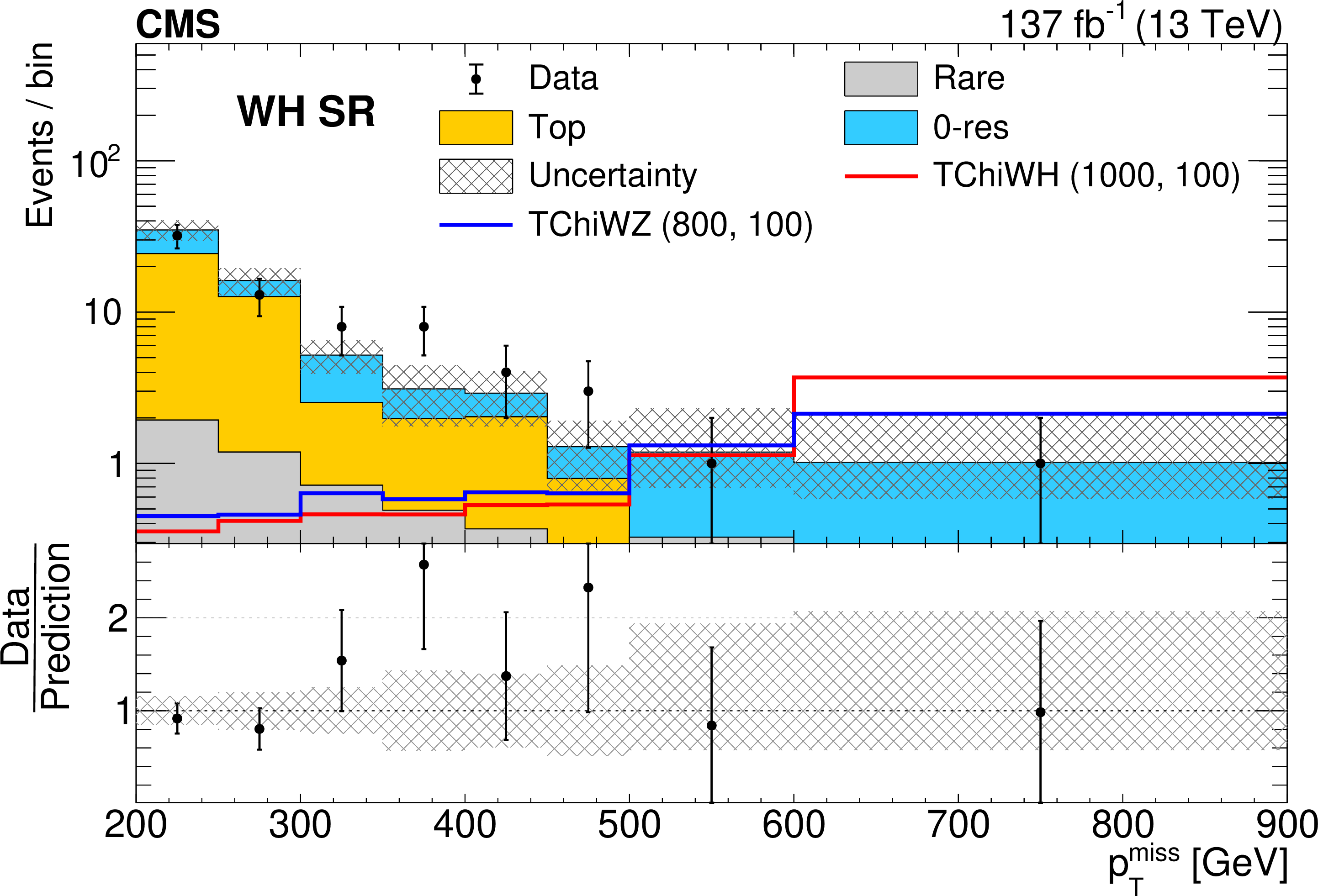
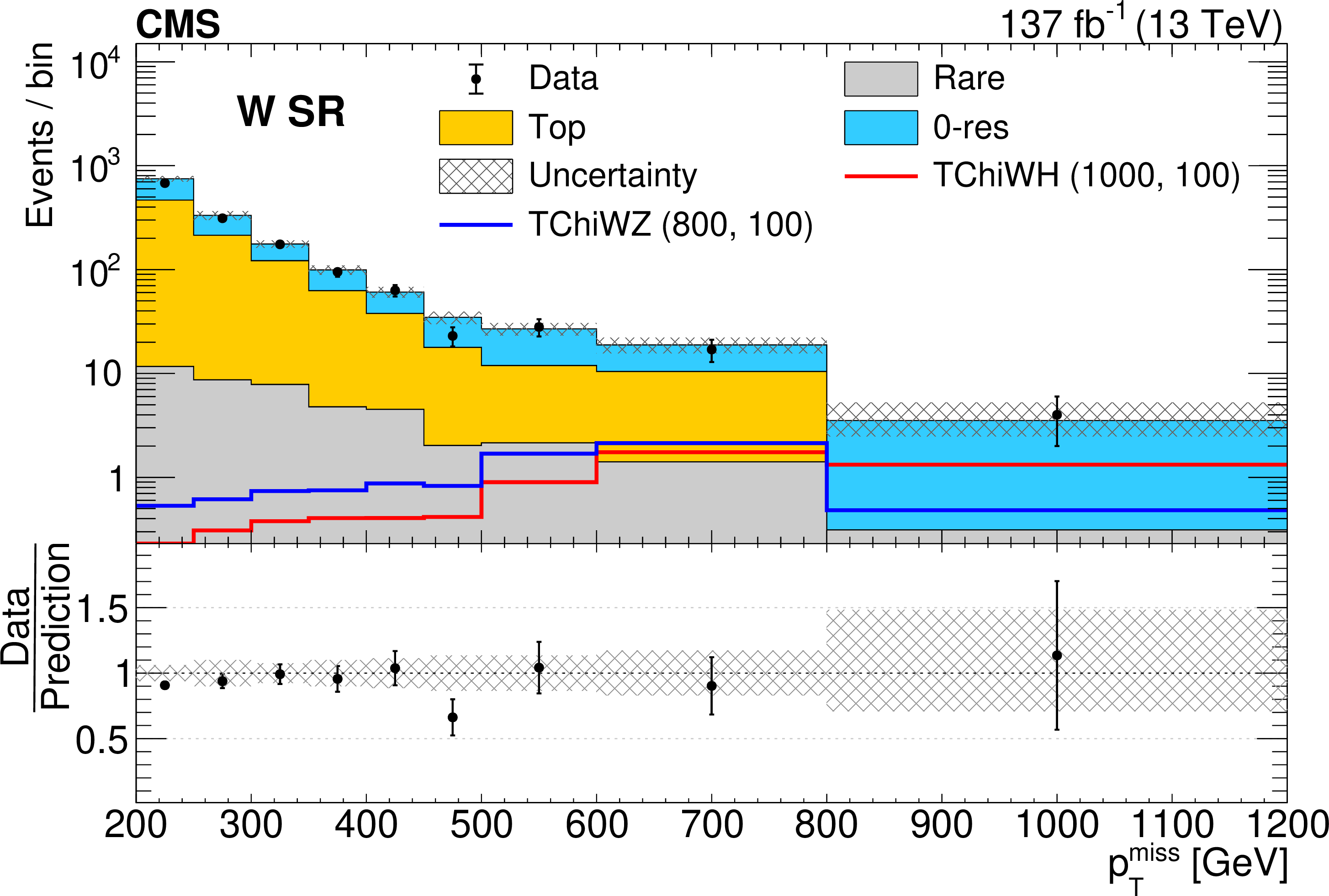
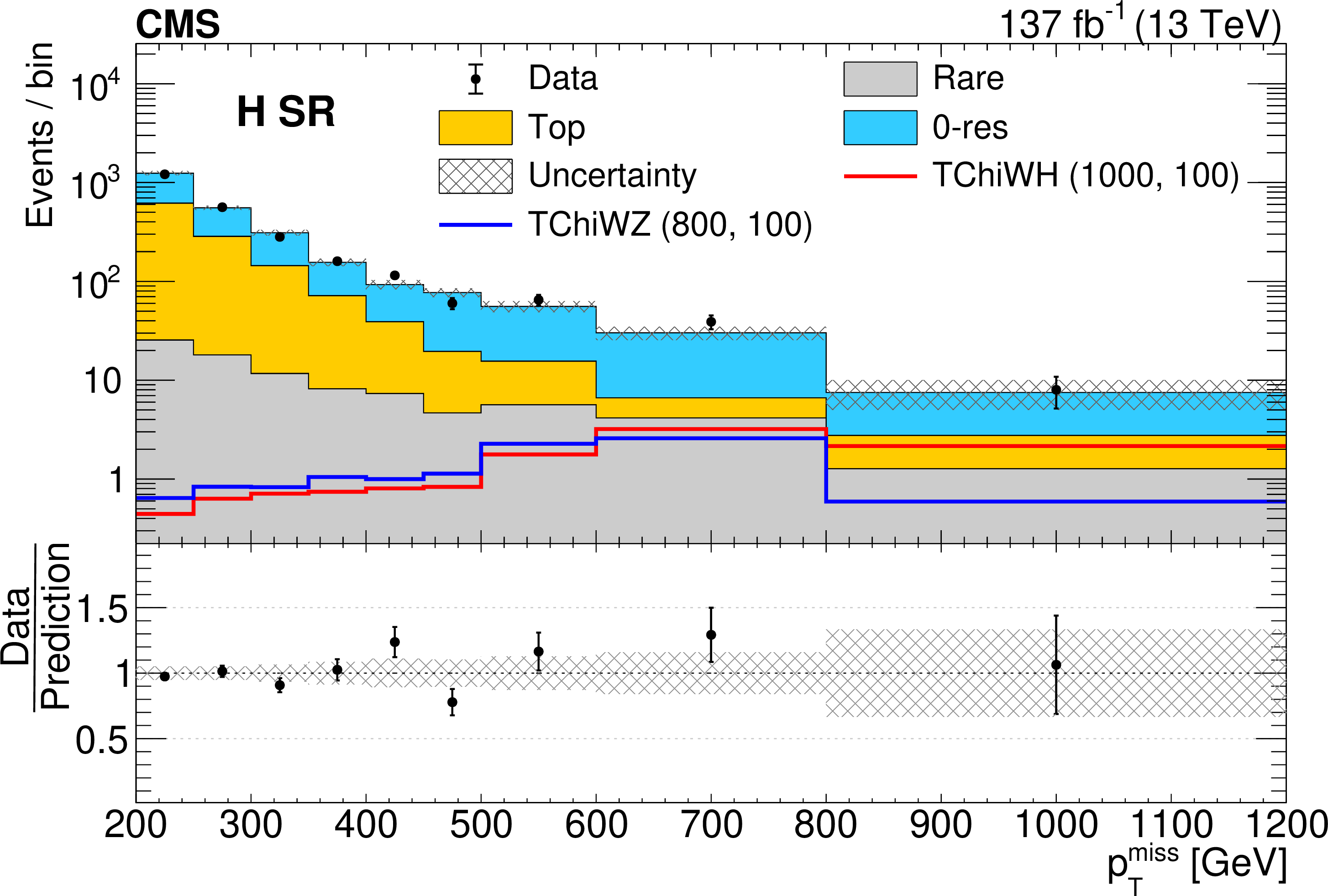
SM background prediction vs. observation in the b-veto SR (upper left), the WH SR (upper right), the W SR (lower left), and the H SR (lower right). The filled stacked histograms show the SM background predictions from the fit to the data in the CRs under the background-only hypothesis. The superimposed open histograms show the expectations for selected signal models, which are denoted in the legend by the name of the model followed by the assumed masses of the NLSP and LSP in GeV. The observed event yields are indicated by black markers. The hatched gray band corresponds to the total uncertainty in the prediction. |

png pdf |
Figure 3-a:
SM background prediction vs. observation in the b-veto SR. The filled stacked histograms show the SM background predictions from the fit to the data in the CRs under the background-only hypothesis. The superimposed open histograms show the expectations for selected signal models, which are denoted in the legend by the name of the model followed by the assumed masses of the NLSP and LSP in GeV. The observed event yields are indicated by black markers. The hatched gray band corresponds to the total uncertainty in the prediction. |
png pdf |
Figure 3-b:
SM background prediction vs. observation in the WH SR. The filled stacked histograms show the SM background predictions from the fit to the data in the CRs under the background-only hypothesis. The superimposed open histograms show the expectations for selected signal models, which are denoted in the legend by the name of the model followed by the assumed masses of the NLSP and LSP in GeV. The observed event yields are indicated by black markers. The hatched gray band corresponds to the total uncertainty in the prediction. |
png pdf |
Figure 3-c:
SM background prediction vs. observation in the W SR. The filled stacked histograms show the SM background predictions from the fit to the data in the CRs under the background-only hypothesis. The superimposed open histograms show the expectations for selected signal models, which are denoted in the legend by the name of the model followed by the assumed masses of the NLSP and LSP in GeV. The observed event yields are indicated by black markers. The hatched gray band corresponds to the total uncertainty in the prediction. |
png pdf |
Figure 3-d:
SM background prediction vs. observation in the H SR. The filled stacked histograms show the SM background predictions from the fit to the data in the CRs under the background-only hypothesis. The superimposed open histograms show the expectations for selected signal models, which are denoted in the legend by the name of the model followed by the assumed masses of the NLSP and LSP in GeV. The observed event yields are indicated by black markers. The hatched gray band corresponds to the total uncertainty in the prediction. |
png pdf |
Figure 4:
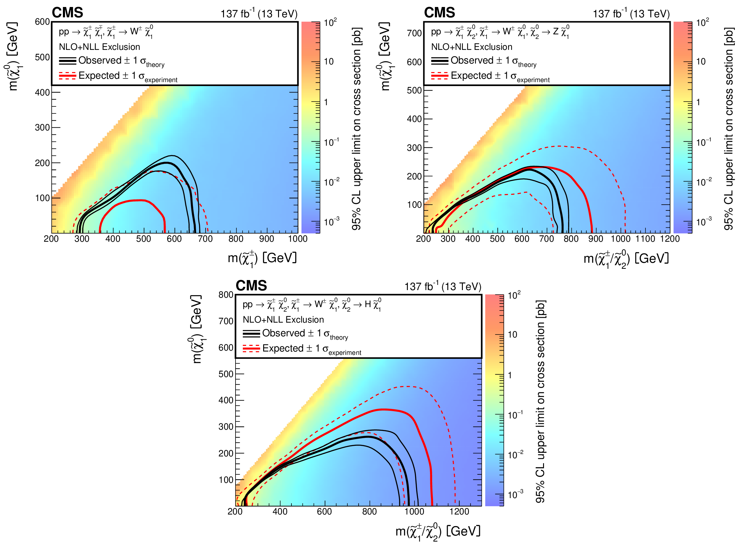
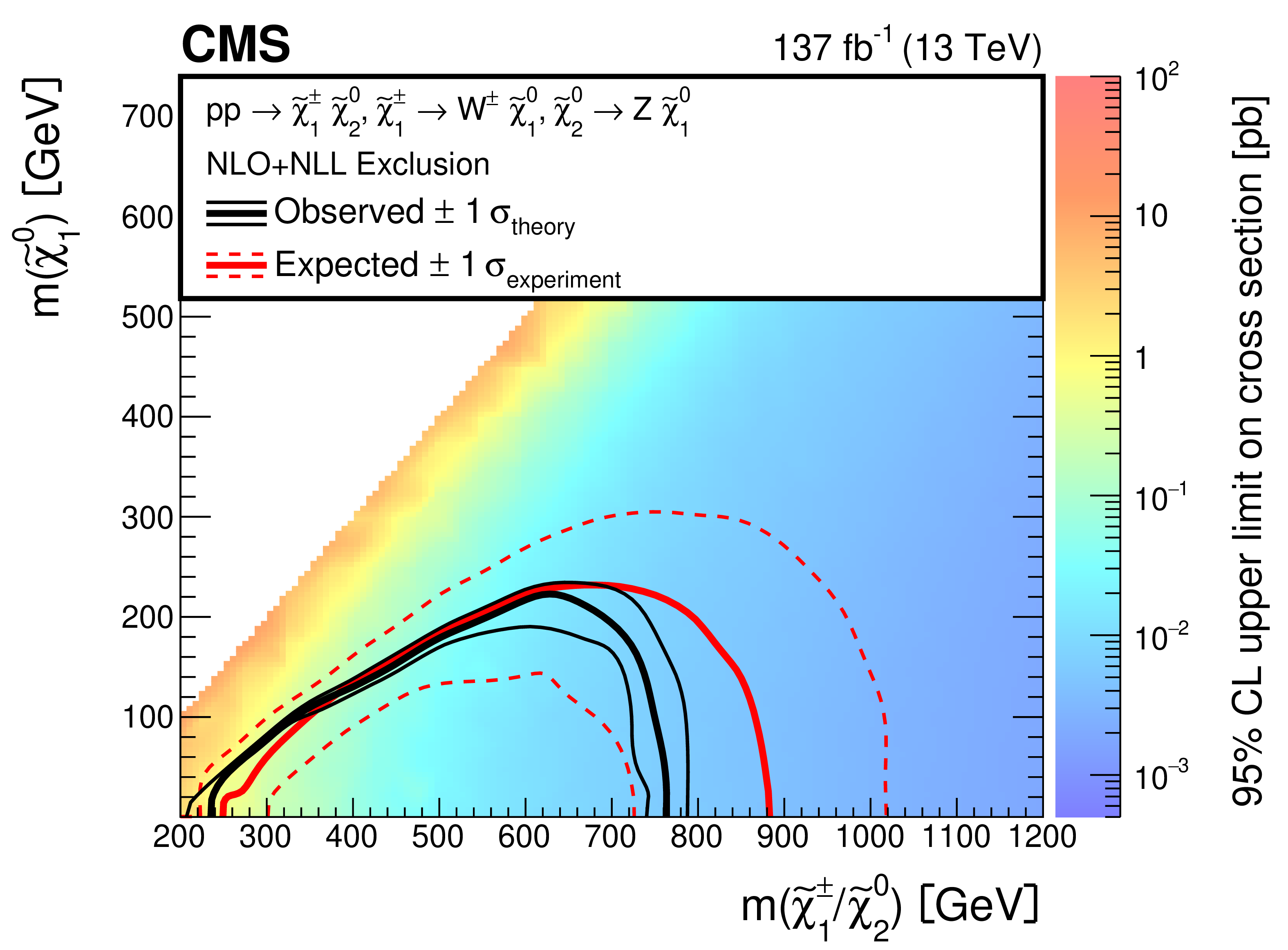
The 95% CL upper limits on the production cross sections for ${\tilde{\chi}^{\pm}_1 \tilde{\chi}^{\mp}_1}$ assuming that each $\tilde{\chi}^{\pm}_1$ decays to a W boson and $\tilde{\chi}^0_1$ (upper left, the TChiWW model) and ${\tilde{\chi}^{\pm}_1 \tilde{\chi}^{0}_2}$ production assuming that the $\tilde{\chi}^{\pm}_1$ decays to a W boson and $\tilde{\chi}^0_1$ and that the $\tilde{\chi}^{0}_2$ decays to a Z boson and $\tilde{\chi}^0_1$ (upper right, the TChiWZ model) or that the $\tilde{\chi}^{0}_2$ decays to a Higgs boson and $\tilde{\chi}^0_1$ (lower, the TChiWH model). The black curves represent the observed exclusion contour and the change in this contour due to variation of these cross sections within their theoretical uncertainties ($\sigma _{\text {theory}}$). The red curves indicate the mean expected exclusion contour and the region containing 68% ($ \pm $1$\sigma _{\text {experiment}}$) of the expected exclusion limits under the background-only hypothesis. The mass exclusion limits are computed assuming wino-like cross sections. |

png pdf root |
Figure 4-a:
The 95% CL upper limits on the production cross sections for ${\tilde{\chi}^{\pm}_1 \tilde{\chi}^{\mp}_1}$ assuming that each $\tilde{\chi}^{\pm}_1$ decays to a W boson and $\tilde{\chi}^0_1$ (TChiWW model). The black curves represent the observed exclusion contour and the change in this contour due to variation of these cross sections within their theoretical uncertainties ($\sigma _{\text {theory}}$). The red curves indicate the mean expected exclusion contour and the region containing 68% ($ \pm $1$\sigma _{\text {experiment}}$) of the expected exclusion limits under the background-only hypothesis. The mass exclusion limits are computed assuming wino-like cross sections. |
png pdf root |
Figure 4-b:
The 95% CL upper limits on the production cross sections for ${\tilde{\chi}^{\pm}_1 \tilde{\chi}^{0}_2}$ assuming that the $\tilde{\chi}^{\pm}_1$ decays to a W boson and $\tilde{\chi}^0_1$ and that the $\tilde{\chi}^{0}_2$ decays to a Z boson and $\tilde{\chi}^0_1$ (TChiWZ model). The black curves represent the observed exclusion contour and the change in this contour due to variation of these cross sections within their theoretical uncertainties ($\sigma _{\text {theory}}$). The red curves indicate the mean expected exclusion contour and the region containing 68% ($ \pm $1$\sigma _{\text {experiment}}$) of the expected exclusion limits under the background-only hypothesis. The mass exclusion limits are computed assuming wino-like cross sections. |

png pdf root |
Figure 4-c:
The 95% CL upper limits on the production cross sections for ${\tilde{\chi}^{\pm}_1 \tilde{\chi}^{0}_2}$ assuming that the $\tilde{\chi}^{\pm}_1$ decays to a W boson and $\tilde{\chi}^0_1$ and that the $\tilde{\chi}^{0}_2$ decays to a Higgs boson and $\tilde{\chi}^0_1$ (TChiWH model). The black curves represent the observed exclusion contour and the change in this contour due to variation of these cross sections within their theoretical uncertainties ($\sigma _{\text {theory}}$). The red curves indicate the mean expected exclusion contour and the region containing 68% ($ \pm $1$\sigma _{\text {experiment}}$) of the expected exclusion limits under the background-only hypothesis. The mass exclusion limits are computed assuming wino-like cross sections. |
png pdf |
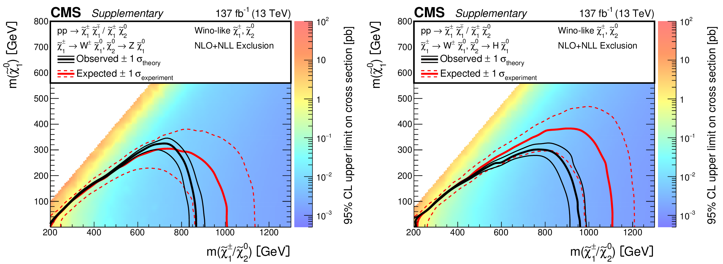
Figure 5:
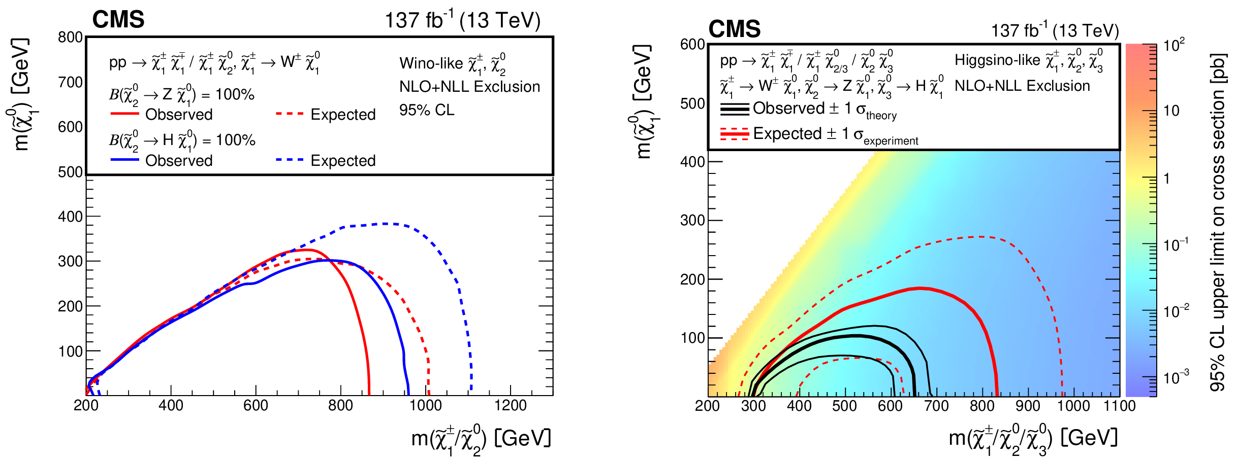
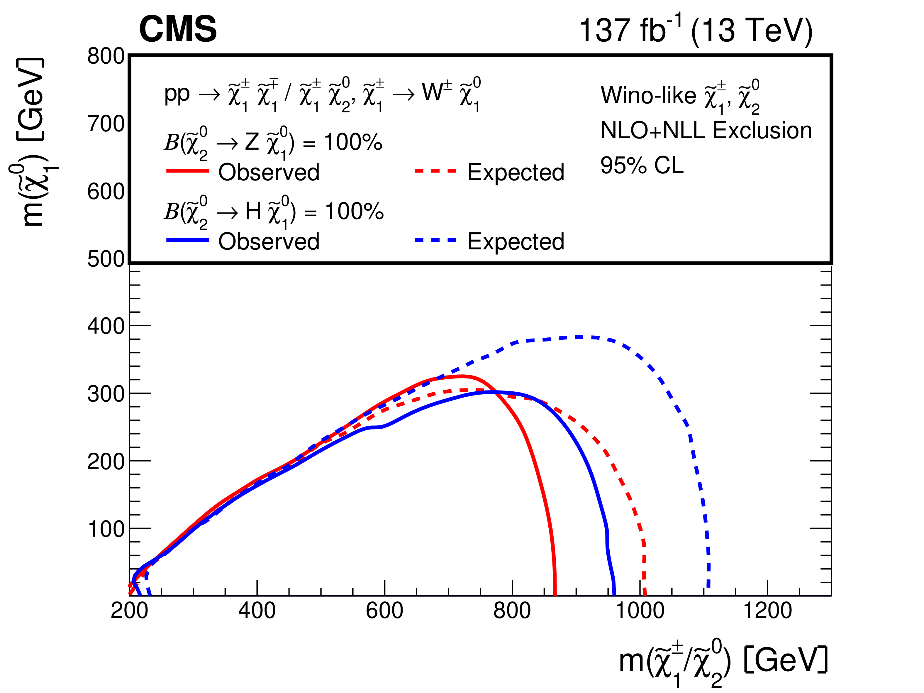
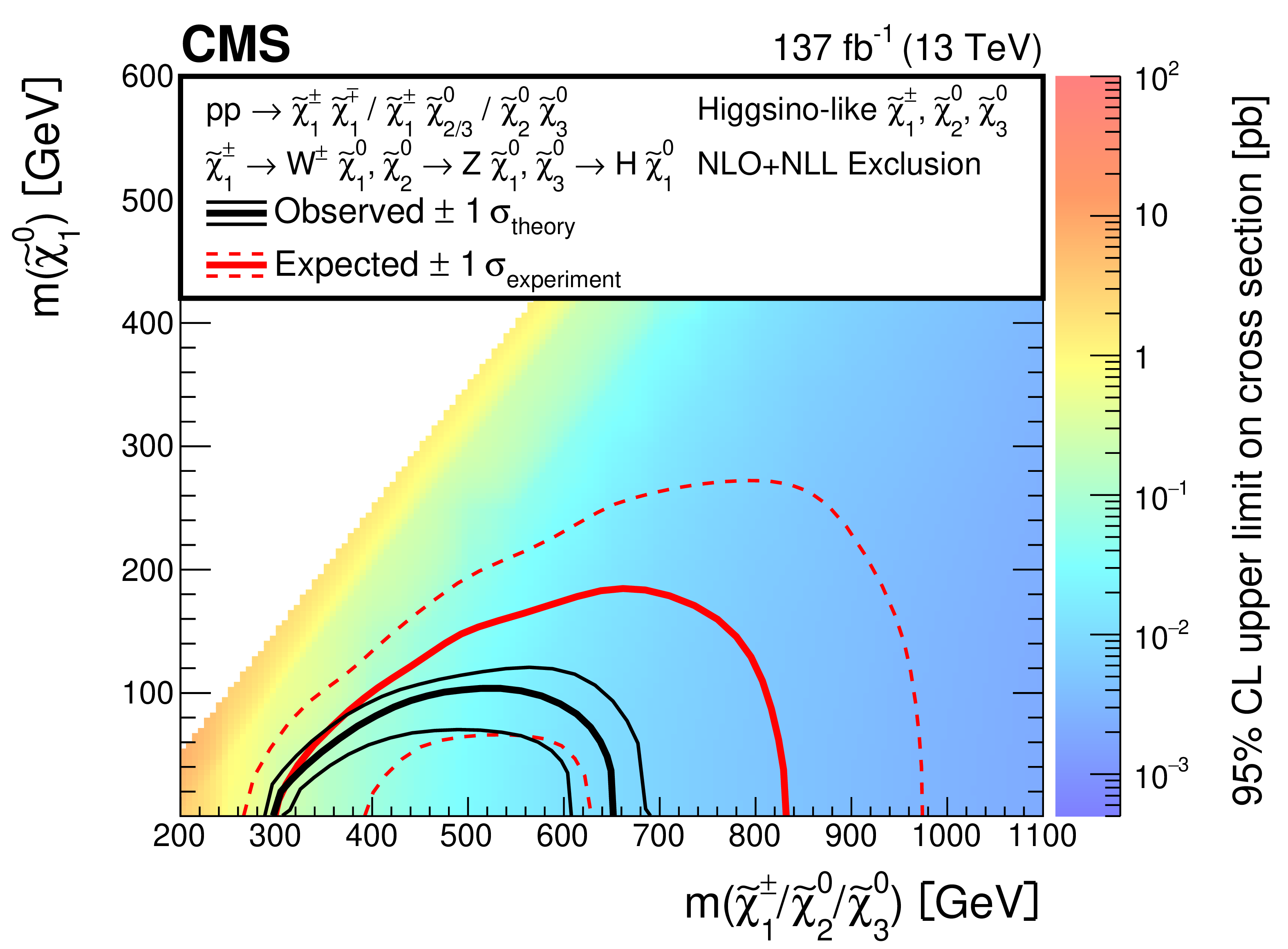
Expected and observed 95% CL exclusion for mass-degenerate wino-like ${\tilde{\chi}^{\pm}_1 \tilde{\chi}^{\mp}_1}$ and ${\tilde{\chi}^{\pm}_1 \tilde{\chi}^{0}_2}$ production (left) and higgsino-like ${\tilde{\chi}^{\pm}_1 \tilde{\chi}^{\mp}_1}$, ${\tilde{\chi}^{\pm}_1 \tilde{\chi}^{0}_2}$, ${\tilde{\chi}^{\pm}_1 \tilde{\chi}^{0}_3}$, and ${\tilde{\chi}^{0}_2 \tilde{\chi}^{0}_3}$ production (right) as functions of the NLSP and LSP masses. The $\tilde{\chi}^{\pm}_1$, $\tilde{\chi}^{0}_2$, and $\tilde{\chi}^{0}_3$ are considered to be mass degenerate. For the higgsino-like case (right), the 95% CL upper limits on the production cross sections are also shown, but they are not shown for the wino-like case (left) because there are two distinct sets of limits depending on the chargino decay mode. |
png pdf root |
Figure 5-a:
Expected and observed 95% CL exclusion for mass-degenerate wino-like ${\tilde{\chi}^{\pm}_1 \tilde{\chi}^{\mp}_1}$ and ${\tilde{\chi}^{\pm}_1 \tilde{\chi}^{0}_2}$ production as functions of the NLSP and LSP masses. The $\tilde{\chi}^{\pm}_1$, $\tilde{\chi}^{0}_2$, and $\tilde{\chi}^{0}_3$ are considered to be mass degenerate. The 95% CL upper limits on the production cross sections are not shown because there are two distinct sets of limits depending on the chargino decay mode. |
png pdf root |
Figure 5-b:
Expected and observed 95% CL exclusion for mass-degenerate higgsino-like ${\tilde{\chi}^{\pm}_1 \tilde{\chi}^{\mp}_1}$, ${\tilde{\chi}^{\pm}_1 \tilde{\chi}^{0}_2}$, ${\tilde{\chi}^{\pm}_1 \tilde{\chi}^{0}_3}$, and ${\tilde{\chi}^{0}_2 \tilde{\chi}^{0}_3}$ production as functions of the NLSP and LSP masses. The $\tilde{\chi}^{\pm}_1$, $\tilde{\chi}^{0}_2$, and $\tilde{\chi}^{0}_3$ are considered to be mass degenerate. The 95% CL upper limits on the production cross sections are also shown. |
| Tables | |

png pdf |
Table 1:
Summary of tagging requirements for the b-veto SR and CRs. Each of these regions includes the baseline selection described in Section 4 and requires zero b-tagged AK4 jets and at least two AK8 jets satisfying 65 $ < {m_{\text {J}}} < $ 105 GeV. The SR and CRs are described in detail in Sections 4.1 and 5.1, respectively. The W and V taggers are described in Section 3. |
png pdf |
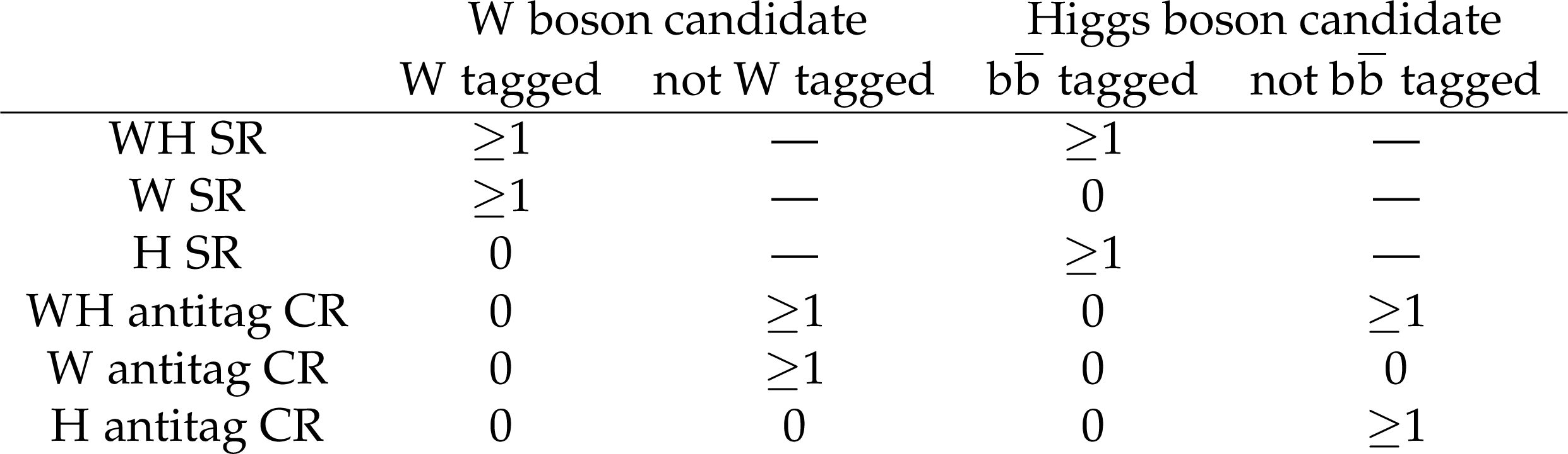
Table 2:
Summary of tagging requirements for the b-tag SRs and CRs. Each of these regions includes the baseline requirements described in Section 4 and requires at least one b-tagged AK4 jet and at least two AK8 jets. The SRs and CRs are described in detail in Sections 4.2 and 5.2, respectively. The ${\mathrm{b} \mathrm{\bar{b}}}$ and W taggers are described in Section 3, and the definitions of W and Higgs boson candidates are given in Section 4.2. In addition to the six regions described in this table, the b-tag predictions also use six single-lepton CRs that are identical except that exactly one charged lepton is required. A dash (--) indicates that no requirement is imposed. |
png pdf |
Table 3:
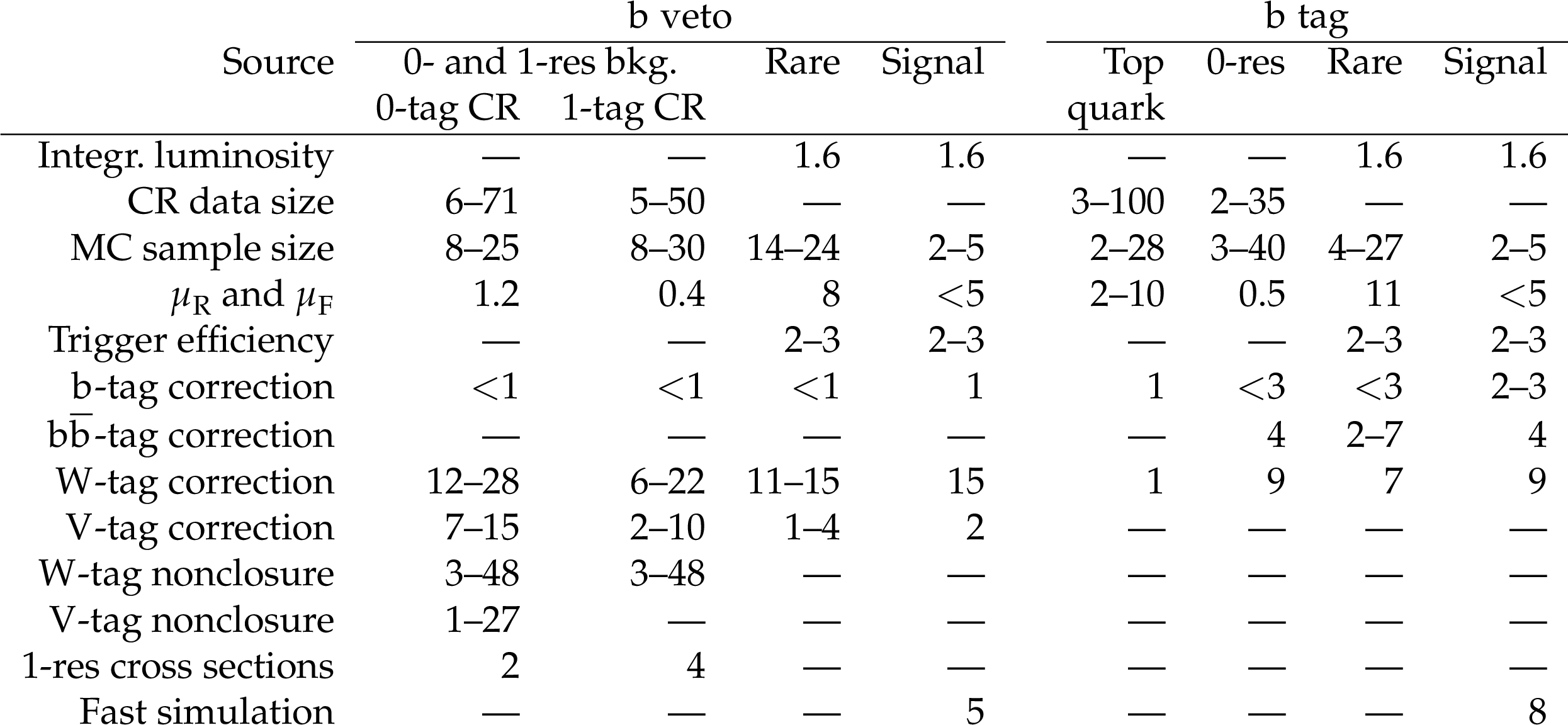
The dominant systematic uncertainties and their effects on event yields (in %) in various SRs. For the 0- and 1-res backgrounds in the b-veto SR, uncertainties are presented separately depending on the CR region used for the estimation. A dash (--) indicates that the source of uncertainty is not applicable. |
| Summary |
|
A search is presented for signatures of electroweak production of charginos and neutralinos in fully hadronic final states. The charginos are assumed to decay to the W boson and the lightest neutralino $\tilde{\chi}^0_1$, and the heavier neutralinos ($\tilde{\chi}^{0}_2$ and $\tilde{\chi}^{0}_3$) are assumed to decay to either the Z or Higgs boson (H) and $\tilde{\chi}^0_1$. The decay products of W, Z, or Higgs bosons are clustered into large-radius jets. These jets are categorized based on their mass and a collection of novel jet-tagging algorithms based on deep neural networks. Four search regions, three that require b tags and one that excludes b tags, are constructed to look for chargino- and neutralino-mediated production of a pair of bosons, WW, WZ, or WH, together with a large transverse momentum imbalance. We consider simplified models in which the charginos $\tilde{\chi}^{\pm}_1$ and the next-to-lightest neutralino $\tilde{\chi}^{0}_2$ are assumed to be the mass-degenerate next-to-lightest supersymmetric particles (NLSPs). The lightest neutralino $\tilde{\chi}^0_1$ is assumed to be bino-like and to be the lightest supersymmetric particle (LSP). No statistically significant excess of events is observed in the data with respect to the expectation from the standard model. Using wino-like pair production cross sections, 95% confidence level mass exclusions are derived. For signals with WW, WZ, or WH boson pairs, the NLSP mass exclusion limit for low-mass LSPs extends up to 670, 760, and 970 GeV, respectively. When we consider models including both wino-like NLSP ${\tilde{\chi}^{\pm}_1\tilde{\chi}^{0}_2}$ and $\tilde{\chi}^{\pm}_1$ pair production under the assumption that either $\tilde{\chi}^{0}_2\to\mathrm{Z}\tilde{\chi}^0_1$ or $\tilde{\chi}^{0}_2\to\mathrm{H}\tilde{\chi}^0_1$, the NLSP mass exclusion extends up to 870 and 960 GeV, respectively. Alternatively, with higgsino-like NLSPs $\tilde{\chi}^{\pm}_1$, $\tilde{\chi}^{0}_2$, and $\tilde{\chi}^{0}_3$, the higgsino masses from 300 to 650 GeV are excluded for low-mass LSPs. These mass exclusions significantly improve on those achieved by searches using leptonic probes of SUSY for high NLSP masses. |
| Additional Figures | |
png pdf |
Additional Figure 1:
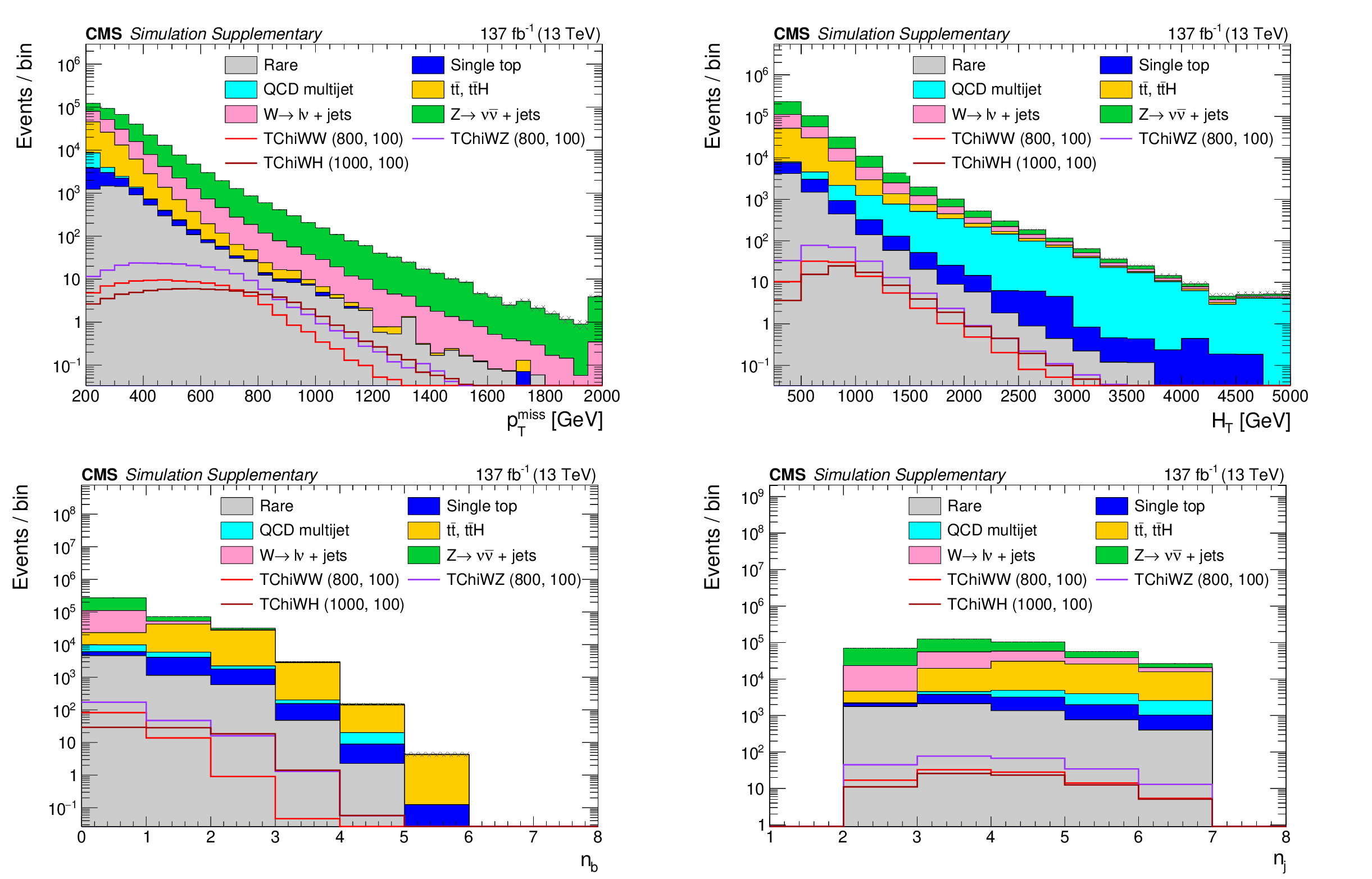
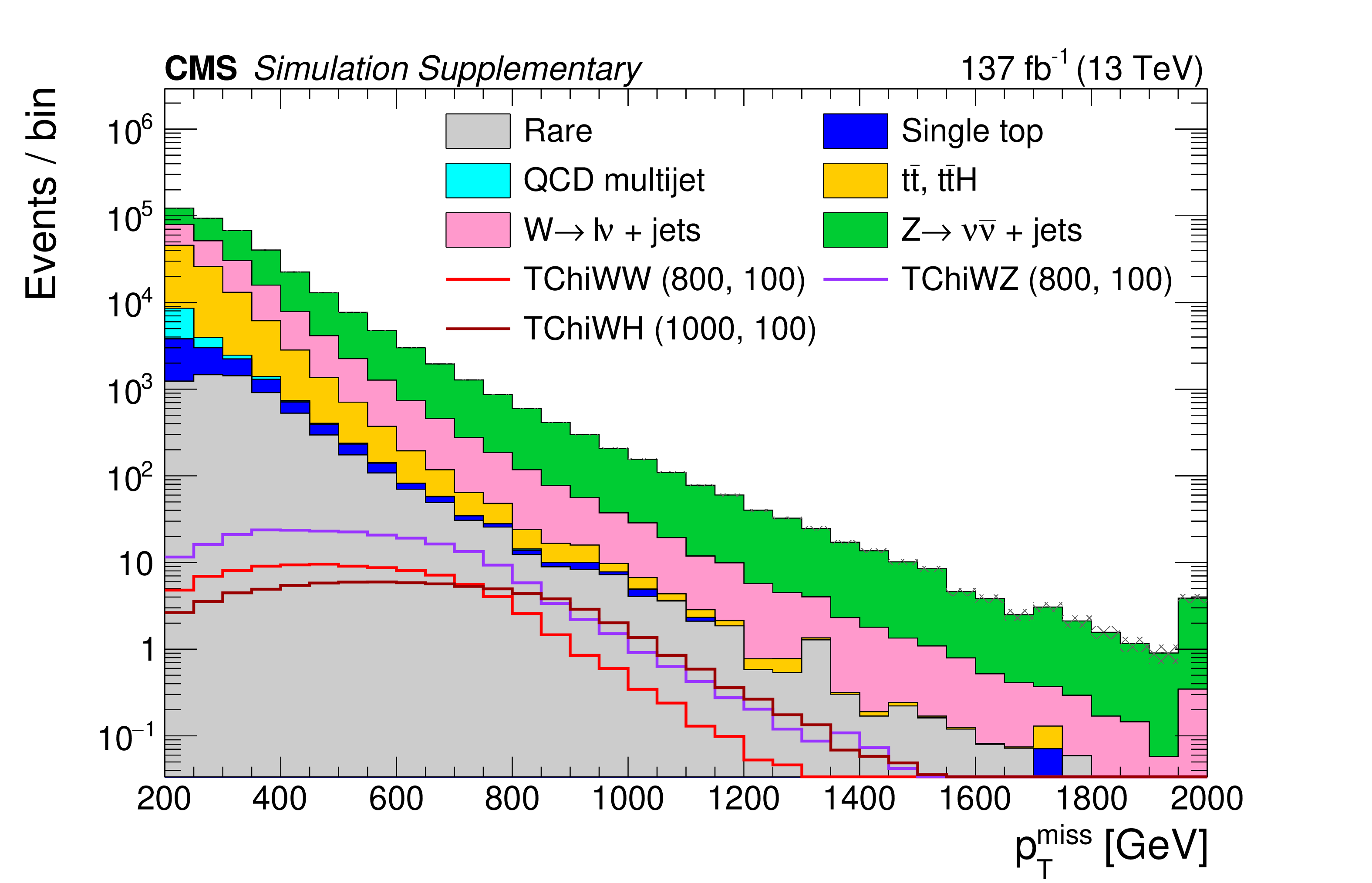
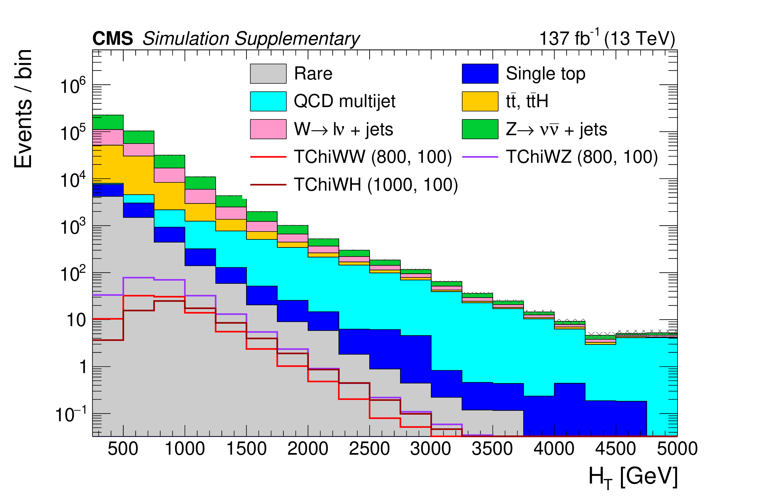
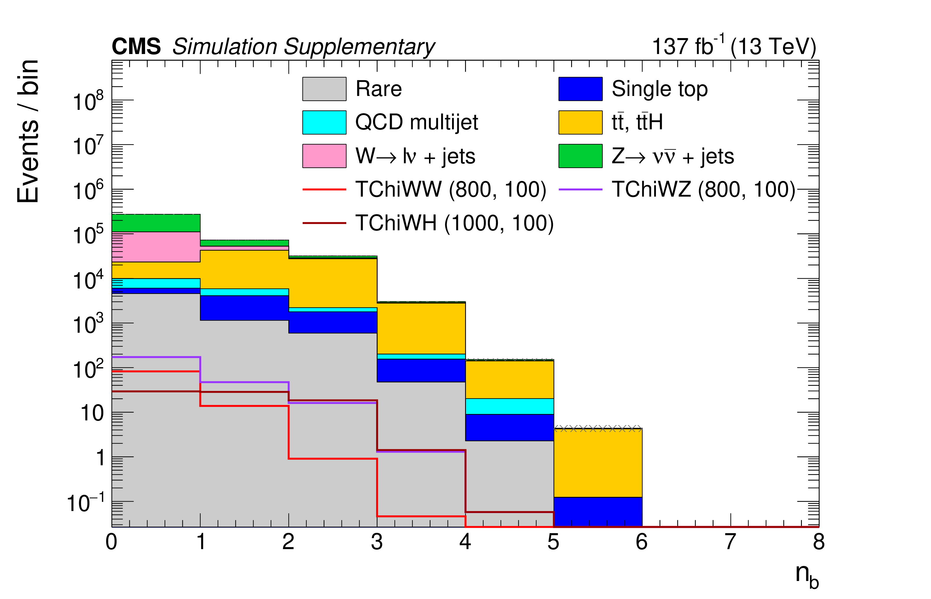
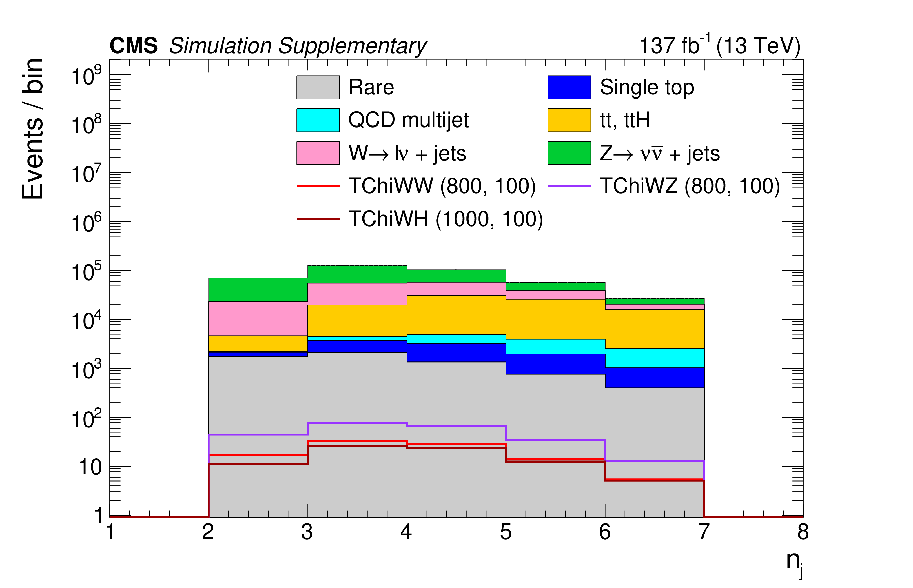
Distributions of $ p_{\mathrm{T}}^\text{miss} $ (a), $ H_{\mathrm{T}} $ (b), the number of b tags (c), and the number of AK4 jets (d) with the baseline selection. The filled histograms show the SM predictions based on simulation, and the open histograms show the expectations for selected signal models, which are denoted in the legend by the name of the model followed by the assumed masses of the NLSP and LSP. |
png pdf |
Additional Figure 1-a:
Distributions of $ p_{\mathrm{T}}^\text{miss} $ (a), $ H_{\mathrm{T}} $ (b), the number of b tags (c), and the number of AK4 jets (d) with the baseline selection. The filled histograms show the SM predictions based on simulation, and the open histograms show the expectations for selected signal models, which are denoted in the legend by the name of the model followed by the assumed masses of the NLSP and LSP. |
png pdf |
Additional Figure 1-b:
Distributions of $ p_{\mathrm{T}}^\text{miss} $ (a), $ H_{\mathrm{T}} $ (b), the number of b tags (c), and the number of AK4 jets (d) with the baseline selection. The filled histograms show the SM predictions based on simulation, and the open histograms show the expectations for selected signal models, which are denoted in the legend by the name of the model followed by the assumed masses of the NLSP and LSP. |
png pdf |
Additional Figure 1-c:
Distributions of $ p_{\mathrm{T}}^\text{miss} $ (a), $ H_{\mathrm{T}} $ (b), the number of b tags (c), and the number of AK4 jets (d) with the baseline selection. The filled histograms show the SM predictions based on simulation, and the open histograms show the expectations for selected signal models, which are denoted in the legend by the name of the model followed by the assumed masses of the NLSP and LSP. |
png pdf |
Additional Figure 1-d:
Distributions of $ p_{\mathrm{T}}^\text{miss} $ (a), $ H_{\mathrm{T}} $ (b), the number of b tags (c), and the number of AK4 jets (d) with the baseline selection. The filled histograms show the SM predictions based on simulation, and the open histograms show the expectations for selected signal models, which are denoted in the legend by the name of the model followed by the assumed masses of the NLSP and LSP. |
png pdf |
Additional Figure 2:
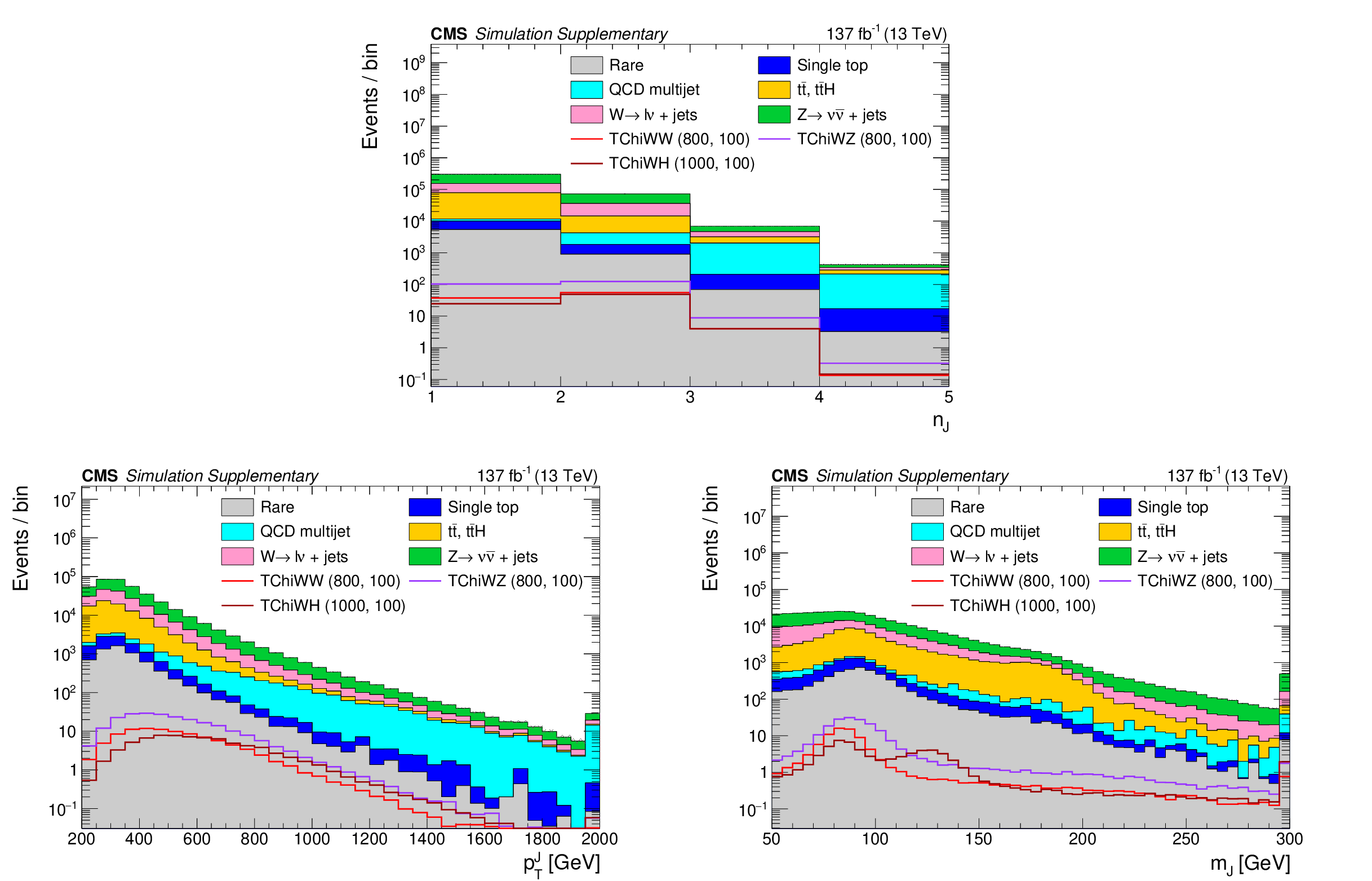
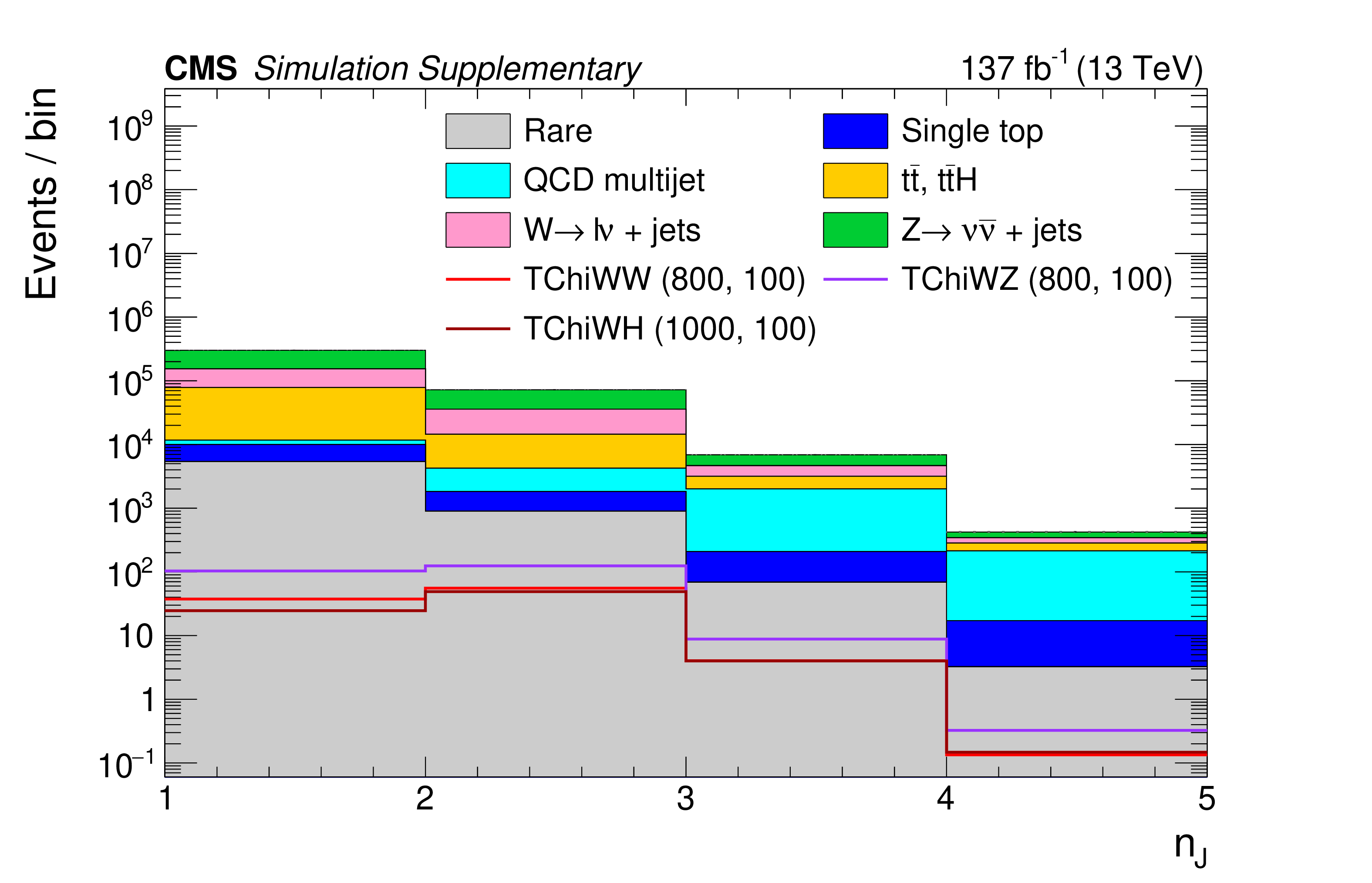
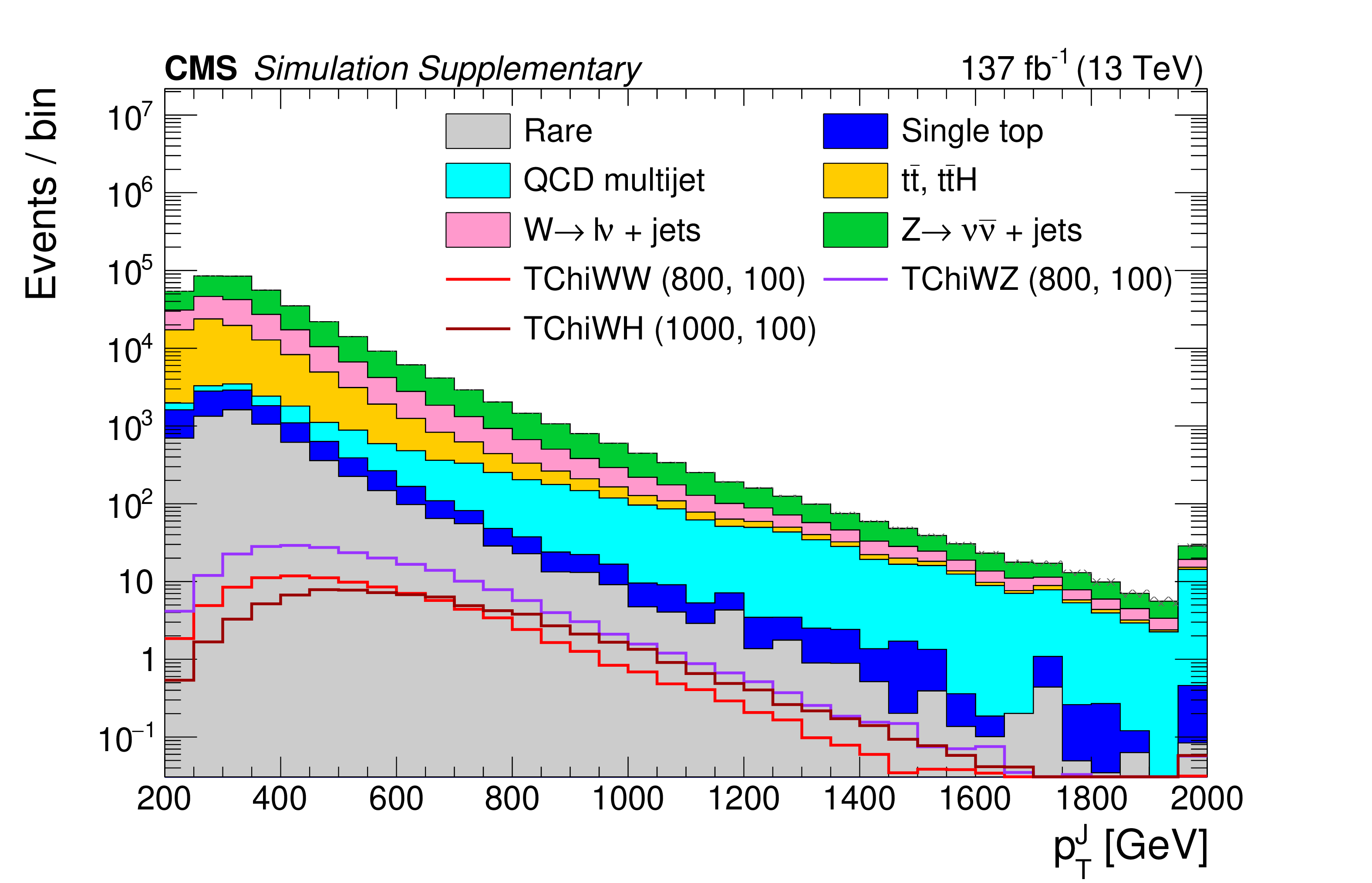
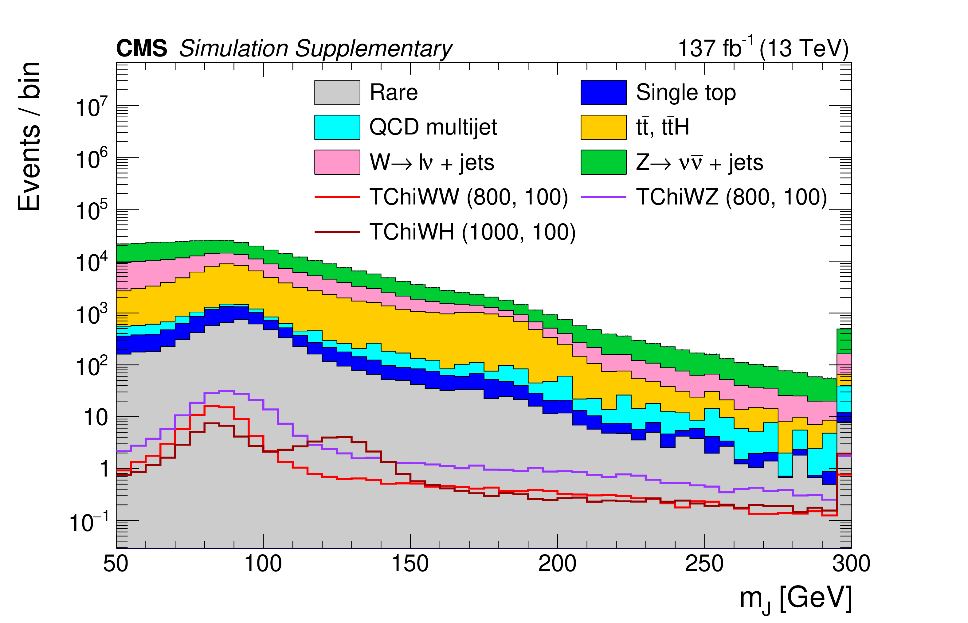
Distributions of the number of AK8 jets (a), the leading AK8 jet $ p_{\mathrm{T}} $ (b), and the soft-drop mass of the leading AK8 jet (c) with the baseline selection. The filled histograms show the SM predictions based on simulation, and the open histograms show the expectations for selected signal models, which are denoted in the legend by the name of the model followed by the assumed masses of the NLSP and LSP. |
png pdf |
Additional Figure 2-a:
Distributions of the number of AK8 jets (a), the leading AK8 jet $ p_{\mathrm{T}} $ (b), and the soft-drop mass of the leading AK8 jet (c) with the baseline selection. The filled histograms show the SM predictions based on simulation, and the open histograms show the expectations for selected signal models, which are denoted in the legend by the name of the model followed by the assumed masses of the NLSP and LSP. |
png pdf |
Additional Figure 2-b:
Distributions of the number of AK8 jets (a), the leading AK8 jet $ p_{\mathrm{T}} $ (b), and the soft-drop mass of the leading AK8 jet (c) with the baseline selection. The filled histograms show the SM predictions based on simulation, and the open histograms show the expectations for selected signal models, which are denoted in the legend by the name of the model followed by the assumed masses of the NLSP and LSP. |
png pdf |
Additional Figure 2-c:
Distributions of the number of AK8 jets (a), the leading AK8 jet $ p_{\mathrm{T}} $ (b), and the soft-drop mass of the leading AK8 jet (c) with the baseline selection. The filled histograms show the SM predictions based on simulation, and the open histograms show the expectations for selected signal models, which are denoted in the legend by the name of the model followed by the assumed masses of the NLSP and LSP. |

png pdf |
Additional Figure 3:
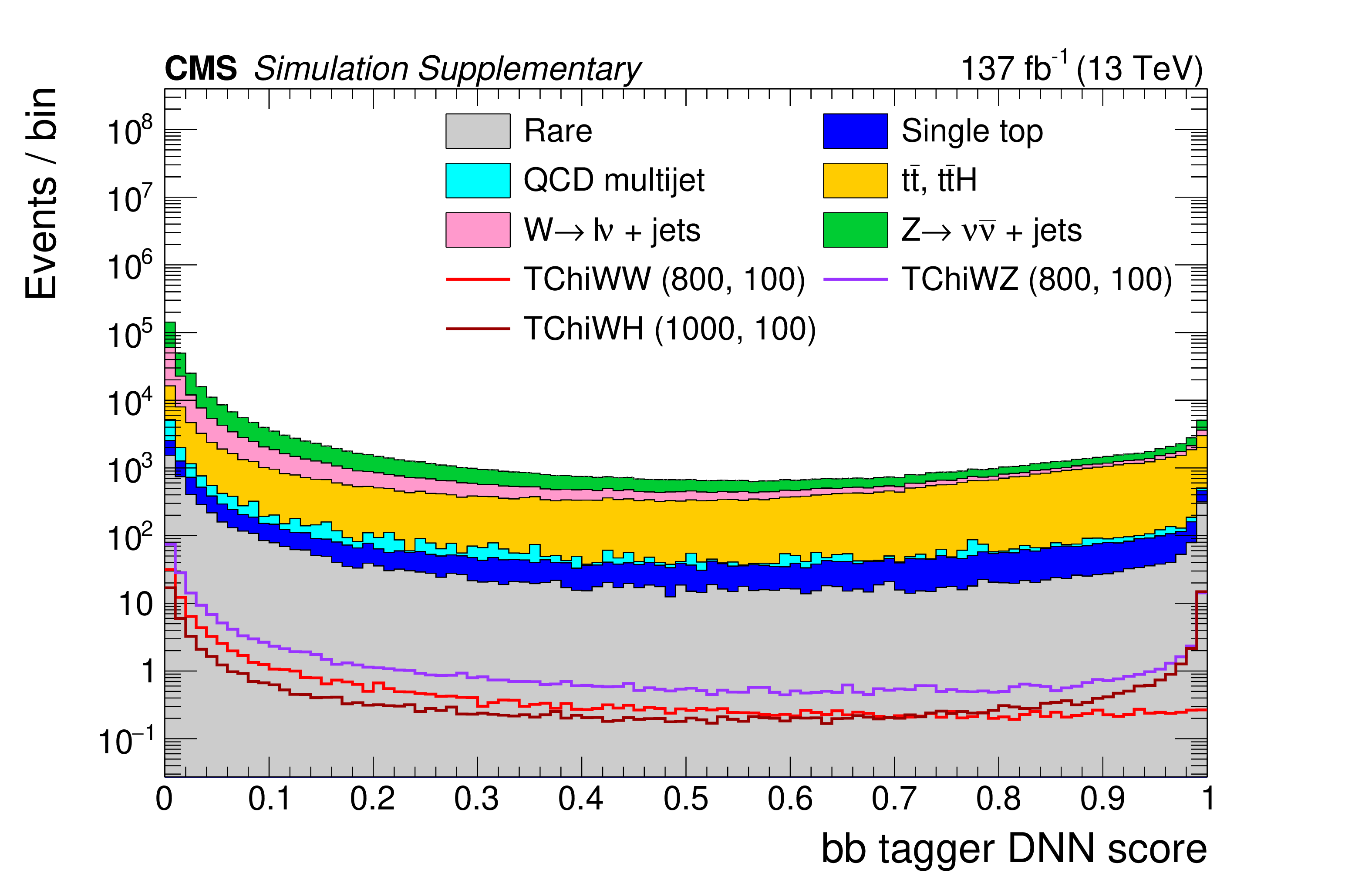
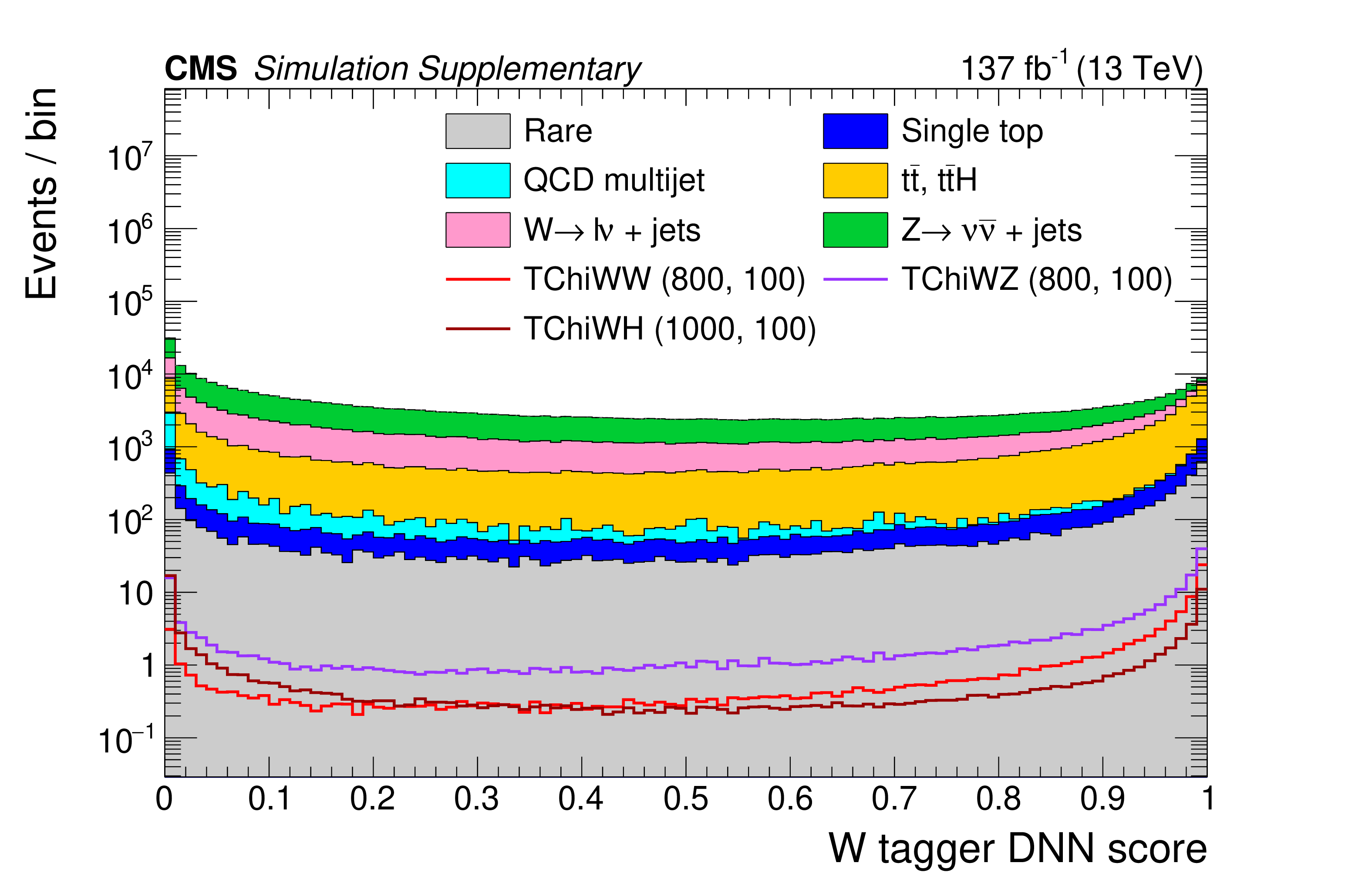
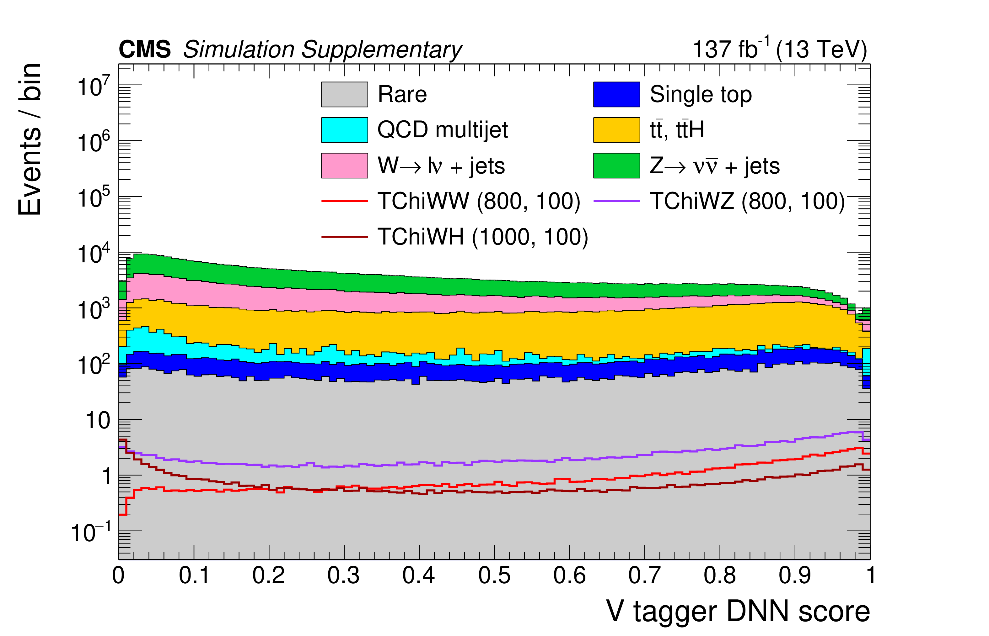
Distributions of the leading AK8 jet's DNN scores for the $ \mathrm{b} \overline{\mathrm{b}} $ tagger (a), the W tagger (b), and the V tagger (c) with the baseline selection. The filled histograms show the SM predictions based on simulation, and the open histograms show the expectations for selected signal models, which are denoted in the legend by the name of the model followed by the assumed masses of the NLSP and LSP. |
png pdf |
Additional Figure 3-a:
Distributions of the leading AK8 jet's DNN scores for the $ \mathrm{b} \overline{\mathrm{b}} $ tagger (a), the W tagger (b), and the V tagger (c) with the baseline selection. The filled histograms show the SM predictions based on simulation, and the open histograms show the expectations for selected signal models, which are denoted in the legend by the name of the model followed by the assumed masses of the NLSP and LSP. |
png pdf |
Additional Figure 3-b:
Distributions of the leading AK8 jet's DNN scores for the $ \mathrm{b} \overline{\mathrm{b}} $ tagger (a), the W tagger (b), and the V tagger (c) with the baseline selection. The filled histograms show the SM predictions based on simulation, and the open histograms show the expectations for selected signal models, which are denoted in the legend by the name of the model followed by the assumed masses of the NLSP and LSP. |
png pdf |
Additional Figure 3-c:
Distributions of the leading AK8 jet's DNN scores for the $ \mathrm{b} \overline{\mathrm{b}} $ tagger (a), the W tagger (b), and the V tagger (c) with the baseline selection. The filled histograms show the SM predictions based on simulation, and the open histograms show the expectations for selected signal models, which are denoted in the legend by the name of the model followed by the assumed masses of the NLSP and LSP. |
png pdf |
Additional Figure 4:
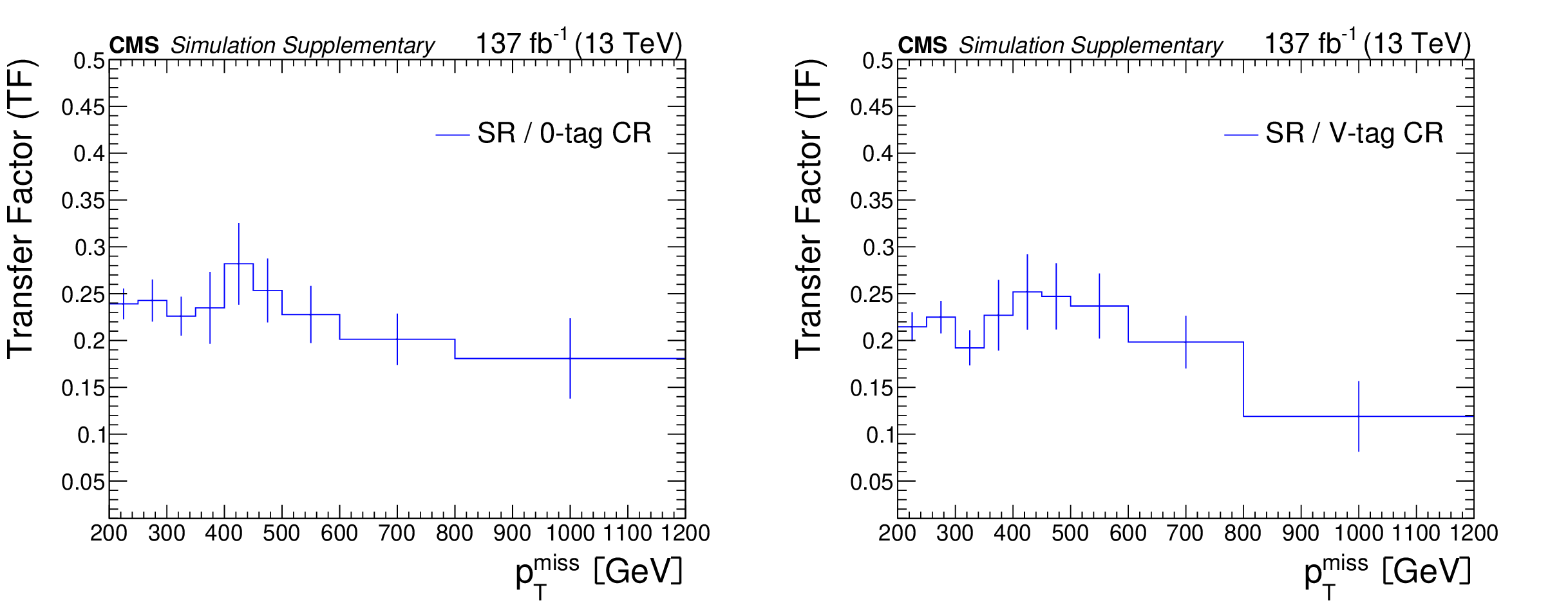
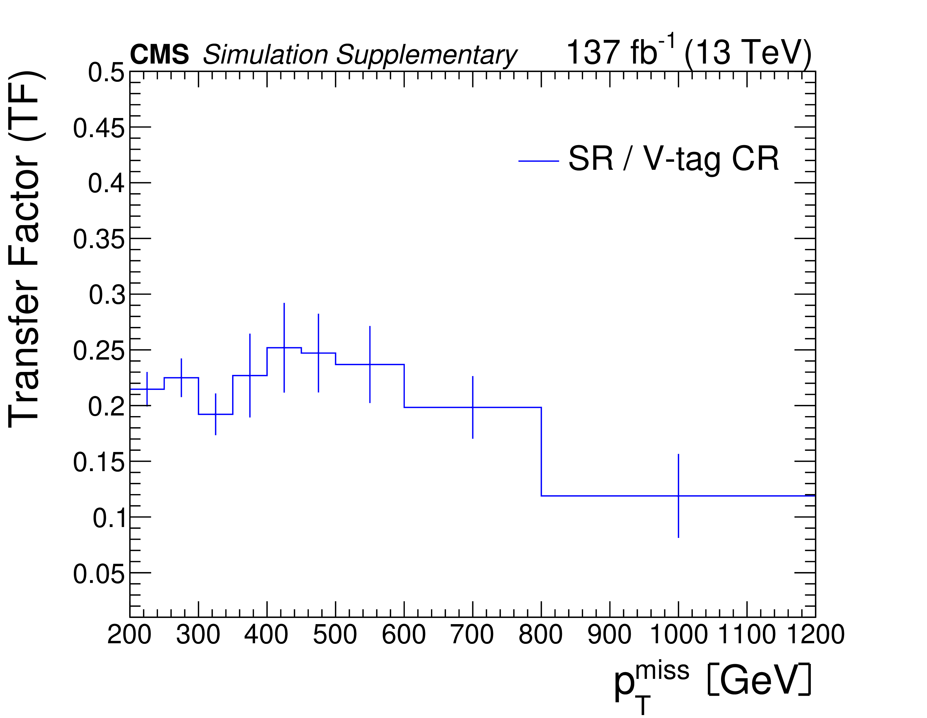
Transfer factors in the b-veto regions, i.e.,, the ratios of the expected yields of the 0- and 1-res backgrounds in different regions: the SR to 0-tag CR ratio (a) and the SR to V-tag CR ratio (b). The vertical error bars indicate the statistical uncertainty in the simulation. |

png pdf |
Additional Figure 4-a:
Transfer factors in the b-veto regions, i.e.,, the ratios of the expected yields of the 0- and 1-res backgrounds in different regions: the SR to 0-tag CR ratio (a) and the SR to V-tag CR ratio (b). The vertical error bars indicate the statistical uncertainty in the simulation. |
png pdf |
Additional Figure 4-b:
Transfer factors in the b-veto regions, i.e.,, the ratios of the expected yields of the 0- and 1-res backgrounds in different regions: the SR to 0-tag CR ratio (a) and the SR to V-tag CR ratio (b). The vertical error bars indicate the statistical uncertainty in the simulation. |
png pdf |
Additional Figure 5:
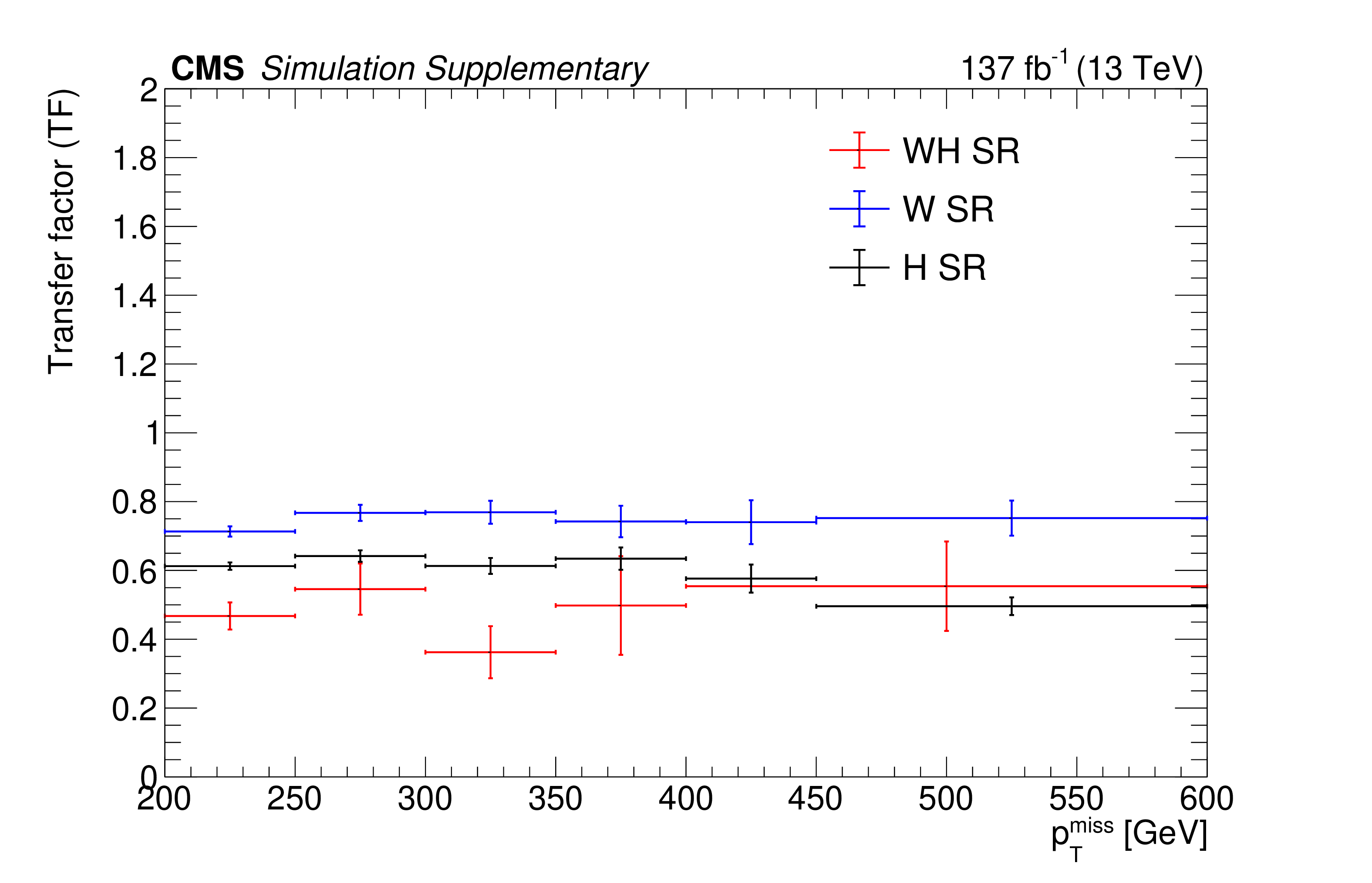
Transfer factors, for extrapolating from 1 $ \ell $ to 0 $ \ell $ regions, as functions of $ p_{\mathrm{T}}^\text{miss} $ in each of the three b-tag SRs. These are computed using simulated events containing top quarks. The vertical error bars indicate the statistical uncertainty in the simulation. |
png pdf |
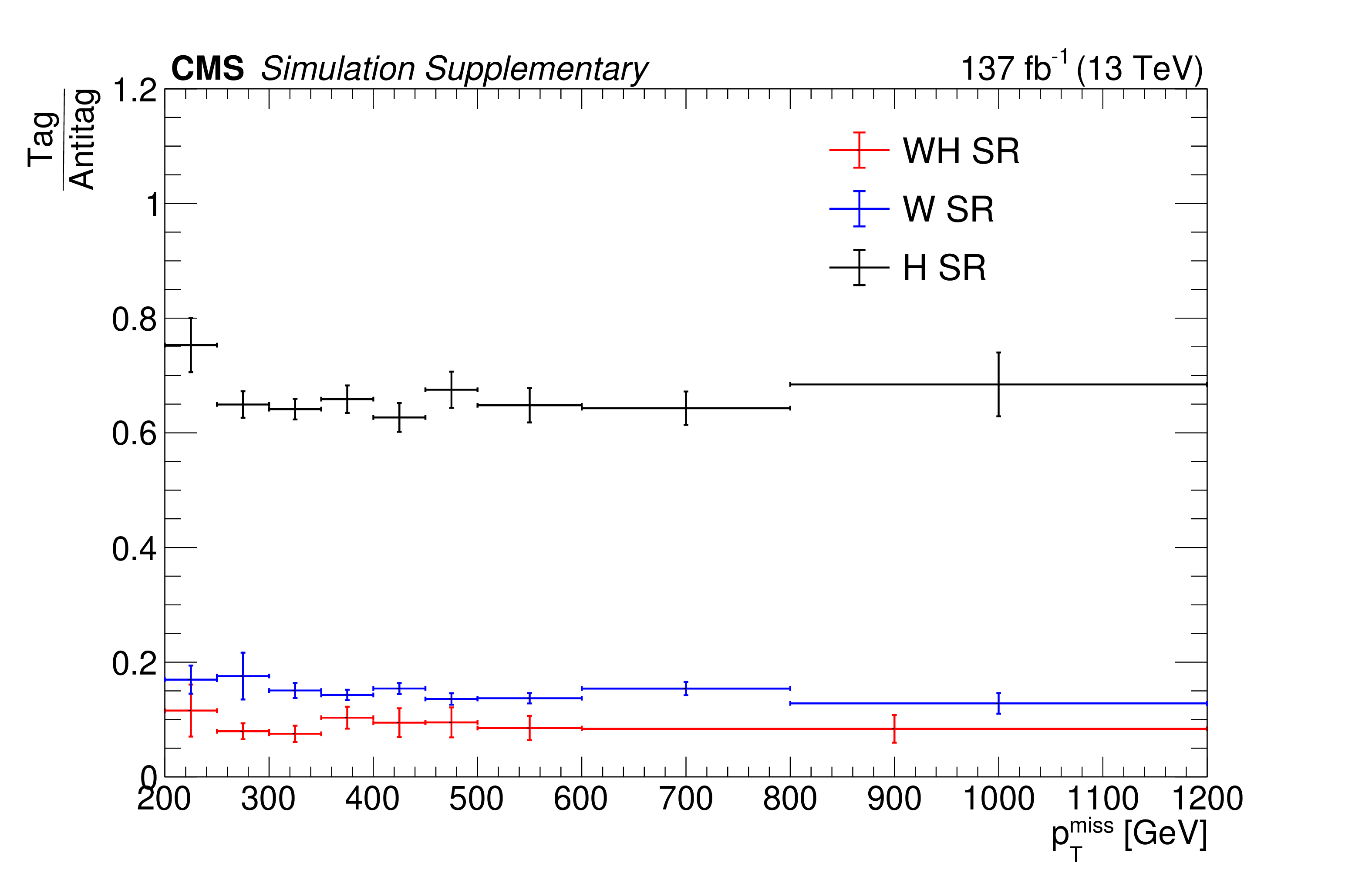
Additional Figure 6:
Tag to antitag ratio as computed from 0-res simulation samples for each of the b-tag SRs and each $ p_{\mathrm{T}}^\text{miss} $ bin. The vertical error bars indicate the statistical uncertainty in the simulation. |

png pdf |
Additional Figure 7:
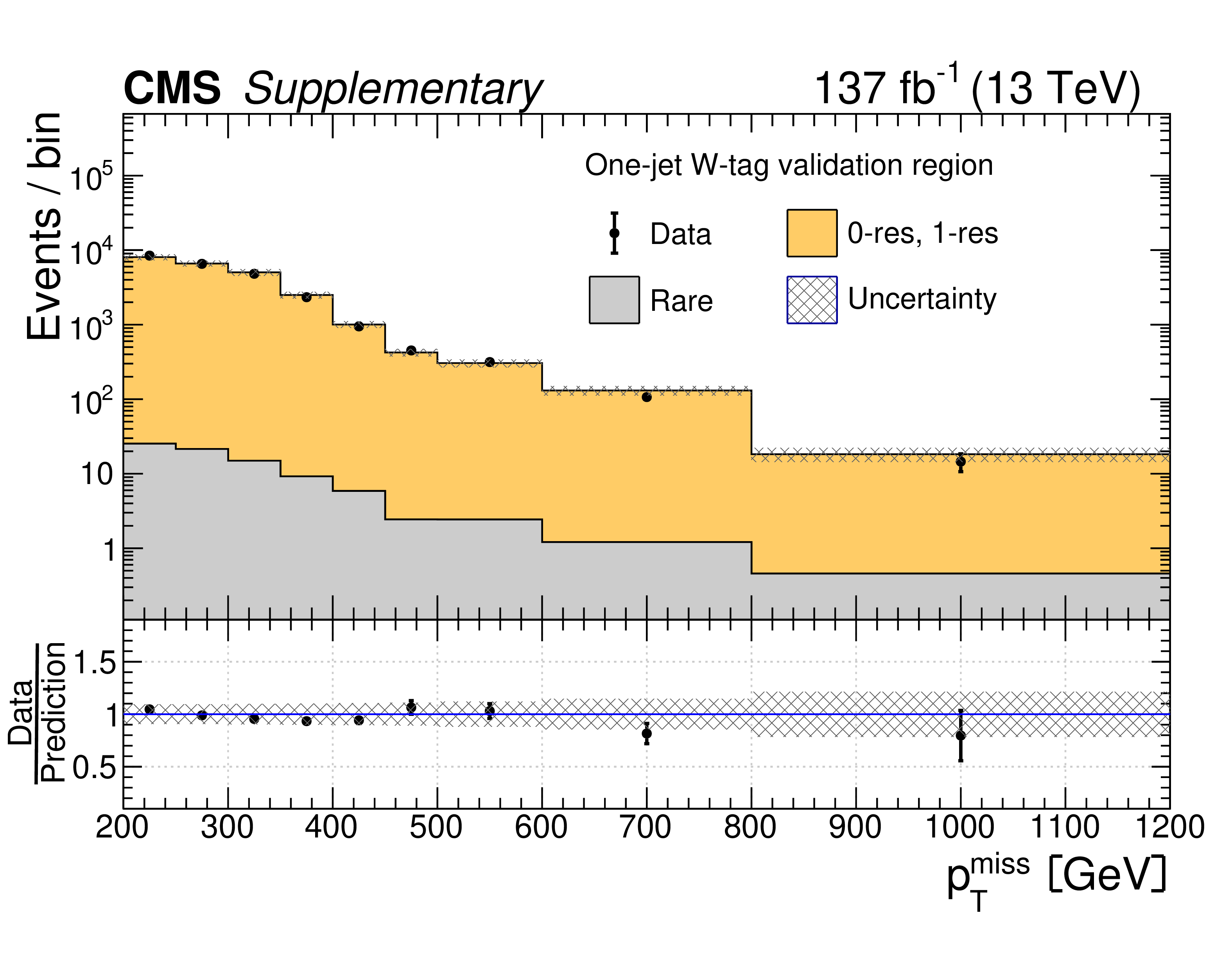
Data yields in the 1-jet W-tag (a) and V-tag (b) validation regions compared to the predicted SM backgrounds as functions of $ p_{\mathrm{T}}^\text{miss} $. In these validation regions, events are required to pass the baseline selection except for the second AK8 jet requirement, and to have only one AK8 jet, which is W or V tagged. The predicted SM 0-res and 1-res backgrounds in each validation region are based on an extrapolation from control regions defined by the inversion of the DNN requirement for the W or V tag. The rare background is taken directly from simulation. The hatched gray bands correspond to the total uncertainty in the prediction. |
png pdf |
Additional Figure 7-a:
Data yields in the 1-jet W-tag (a) and V-tag (b) validation regions compared to the predicted SM backgrounds as functions of $ p_{\mathrm{T}}^\text{miss} $. In these validation regions, events are required to pass the baseline selection except for the second AK8 jet requirement, and to have only one AK8 jet, which is W or V tagged. The predicted SM 0-res and 1-res backgrounds in each validation region are based on an extrapolation from control regions defined by the inversion of the DNN requirement for the W or V tag. The rare background is taken directly from simulation. The hatched gray bands correspond to the total uncertainty in the prediction. |

png pdf |
Additional Figure 7-b:
Data yields in the 1-jet W-tag (a) and V-tag (b) validation regions compared to the predicted SM backgrounds as functions of $ p_{\mathrm{T}}^\text{miss} $. In these validation regions, events are required to pass the baseline selection except for the second AK8 jet requirement, and to have only one AK8 jet, which is W or V tagged. The predicted SM 0-res and 1-res backgrounds in each validation region are based on an extrapolation from control regions defined by the inversion of the DNN requirement for the W or V tag. The rare background is taken directly from simulation. The hatched gray bands correspond to the total uncertainty in the prediction. |
png pdf |
Additional Figure 8:
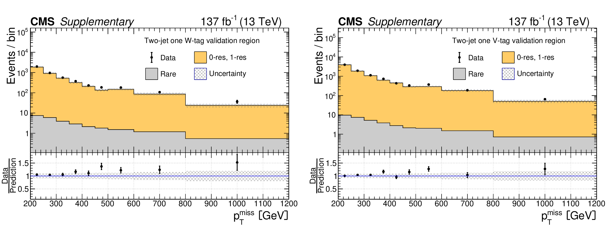
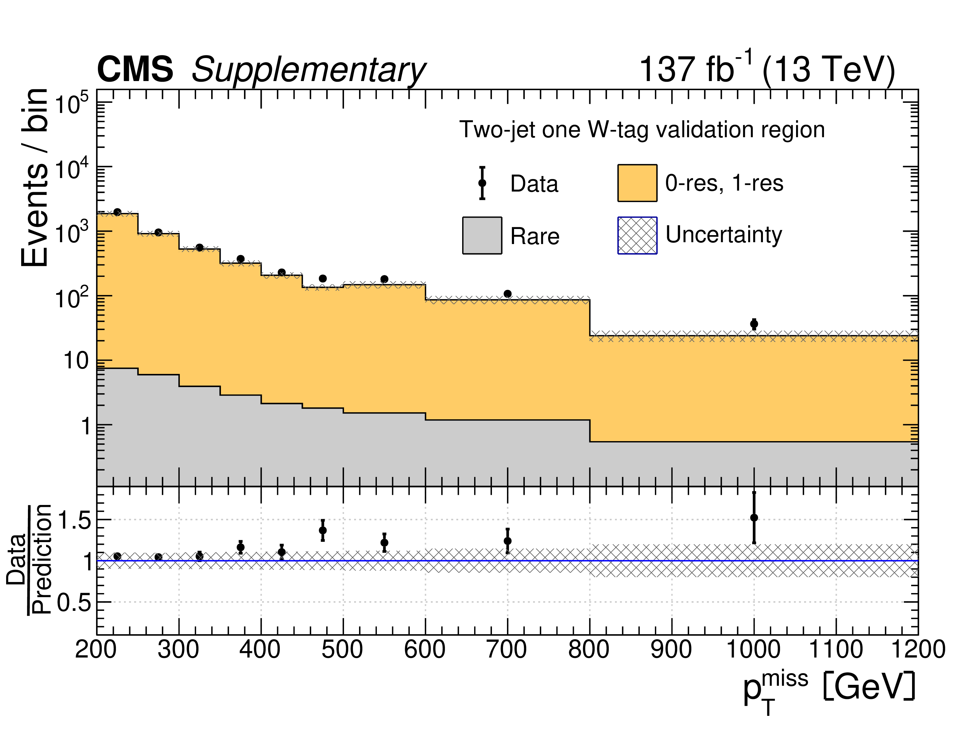
Data yields in the 2-jet, 1-tag validation regions, the W-tag region (a) and the V-tag region (b), compared to the predicted SM backgrounds as functions of $ p_{\mathrm{T}}^\text{miss} $. In these validation regions, events are required to pass the baseline selection including the requirement of having at least two AK8 jets, but only one AK8 jet may pass the WZ mass requirement of 65 $ < m_{\text{J}} < $ 105 GeV, and only one AK8 jet is permitted to be W or V tagged. The predicted SM 0-res and 1-res backgrounds in each validation region are based on an extrapolation from control regions defined by the inversion of the DNN requirement for the W or V tag. The rare background is taken directly from simulation. The deviation from unity of the ratio of the data yields to the SM predictions in each of these validation regions is used to extract the non-closure corrections for the W and V taggers as discussed in the main text, and the full size of the correction is assigned as its uncertainty. The hatched gray bands correspond to the total uncertainty in the prediction. |
png pdf |
Additional Figure 8-a:
Data yields in the 2-jet, 1-tag validation regions, the W-tag region (a) and the V-tag region (b), compared to the predicted SM backgrounds as functions of $ p_{\mathrm{T}}^\text{miss} $. In these validation regions, events are required to pass the baseline selection including the requirement of having at least two AK8 jets, but only one AK8 jet may pass the WZ mass requirement of 65 $ < m_{\text{J}} < $ 105 GeV, and only one AK8 jet is permitted to be W or V tagged. The predicted SM 0-res and 1-res backgrounds in each validation region are based on an extrapolation from control regions defined by the inversion of the DNN requirement for the W or V tag. The rare background is taken directly from simulation. The deviation from unity of the ratio of the data yields to the SM predictions in each of these validation regions is used to extract the non-closure corrections for the W and V taggers as discussed in the main text, and the full size of the correction is assigned as its uncertainty. The hatched gray bands correspond to the total uncertainty in the prediction. |

png pdf |
Additional Figure 8-b:
Data yields in the 2-jet, 1-tag validation regions, the W-tag region (a) and the V-tag region (b), compared to the predicted SM backgrounds as functions of $ p_{\mathrm{T}}^\text{miss} $. In these validation regions, events are required to pass the baseline selection including the requirement of having at least two AK8 jets, but only one AK8 jet may pass the WZ mass requirement of 65 $ < m_{\text{J}} < $ 105 GeV, and only one AK8 jet is permitted to be W or V tagged. The predicted SM 0-res and 1-res backgrounds in each validation region are based on an extrapolation from control regions defined by the inversion of the DNN requirement for the W or V tag. The rare background is taken directly from simulation. The deviation from unity of the ratio of the data yields to the SM predictions in each of these validation regions is used to extract the non-closure corrections for the W and V taggers as discussed in the main text, and the full size of the correction is assigned as its uncertainty. The hatched gray bands correspond to the total uncertainty in the prediction. |
png pdf |
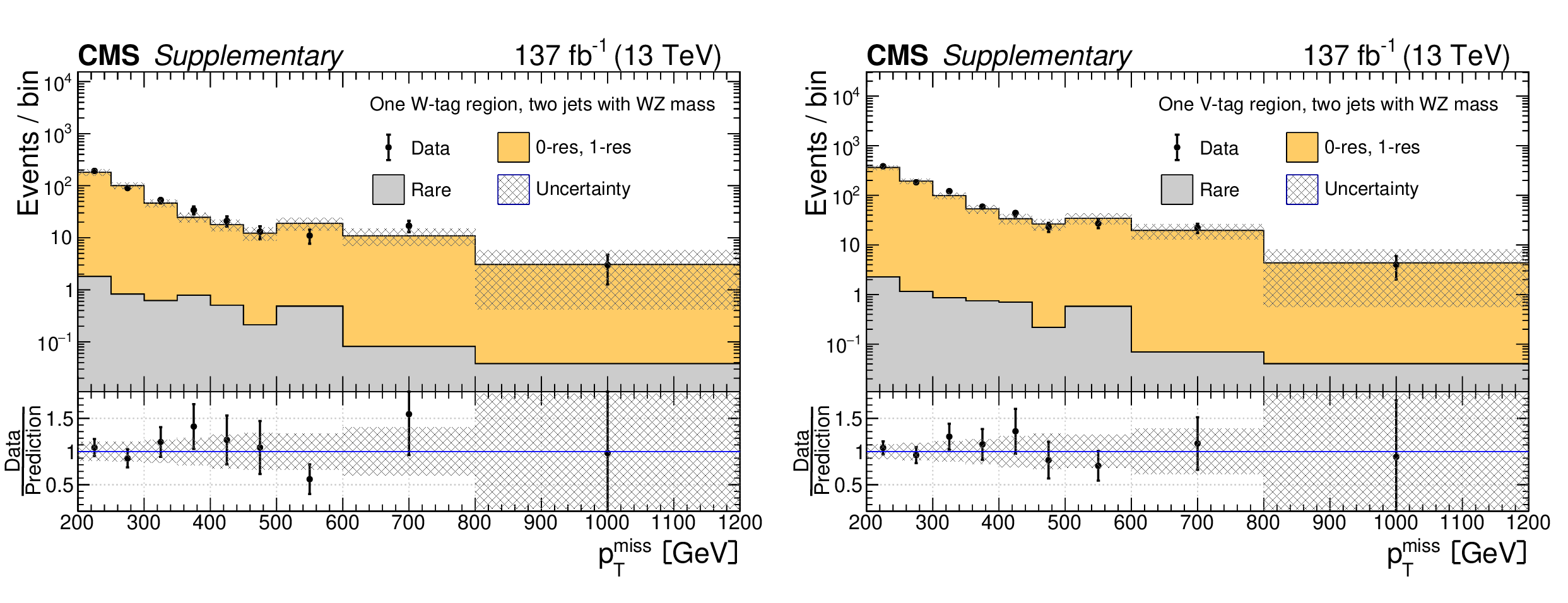
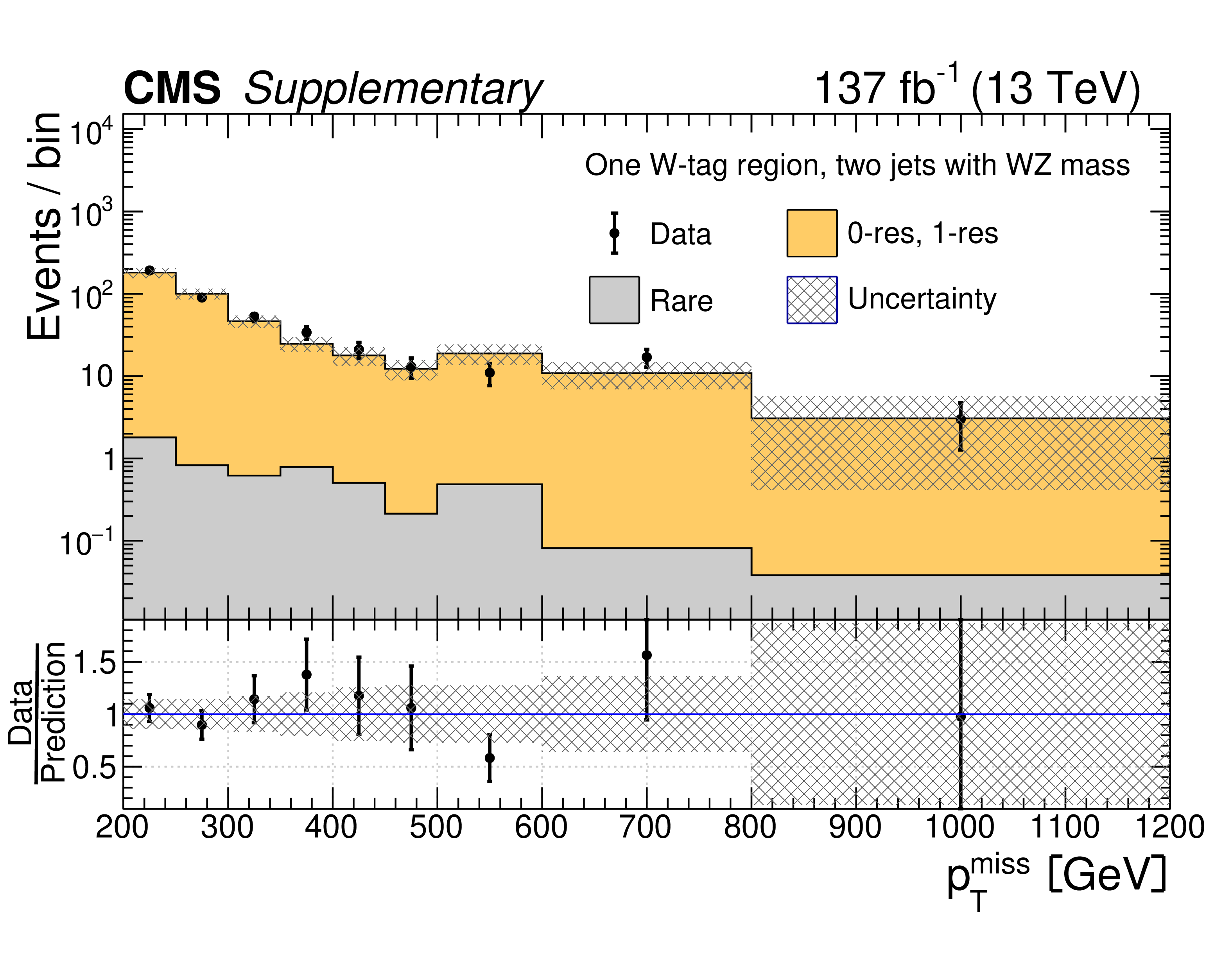
Additional Figure 9:
Data yields in the one W-tag region (a) and one V-tag region (b) compared to the predicted SM backgrounds as functions of $ p_{\mathrm{T}}^\text{miss} $. In these regions, events are required to pass the baseline selection including the requirement of having at least two AK8 jets, at least two AK8 jets must pass the WZ mass requirement of 65 $ < m_{\text{J}} < $ 105 GeV, but only one AK8 jet is permitted to be W or V tagged. The predicted SM 0-res and 1-res backgrounds in each validation region are based on an extrapolation from the 0-tag control region, in which events have at least two AK8 jets passing the WZ mass requirement of 65 $ < m_{\text{J}} < $ 105 GeV but none of them pass the DNN requirements for the W or V taggers. The rare background is taken directly from simulation. The hatched gray bands correspond to the total uncertainty in the prediction. |
png pdf |
Additional Figure 9-a:
Data yields in the one W-tag region (a) and one V-tag region (b) compared to the predicted SM backgrounds as functions of $ p_{\mathrm{T}}^\text{miss} $. In these regions, events are required to pass the baseline selection including the requirement of having at least two AK8 jets, at least two AK8 jets must pass the WZ mass requirement of 65 $ < m_{\text{J}} < $ 105 GeV, but only one AK8 jet is permitted to be W or V tagged. The predicted SM 0-res and 1-res backgrounds in each validation region are based on an extrapolation from the 0-tag control region, in which events have at least two AK8 jets passing the WZ mass requirement of 65 $ < m_{\text{J}} < $ 105 GeV but none of them pass the DNN requirements for the W or V taggers. The rare background is taken directly from simulation. The hatched gray bands correspond to the total uncertainty in the prediction. |

png pdf |
Additional Figure 9-b:
Data yields in the one W-tag region (a) and one V-tag region (b) compared to the predicted SM backgrounds as functions of $ p_{\mathrm{T}}^\text{miss} $. In these regions, events are required to pass the baseline selection including the requirement of having at least two AK8 jets, at least two AK8 jets must pass the WZ mass requirement of 65 $ < m_{\text{J}} < $ 105 GeV, but only one AK8 jet is permitted to be W or V tagged. The predicted SM 0-res and 1-res backgrounds in each validation region are based on an extrapolation from the 0-tag control region, in which events have at least two AK8 jets passing the WZ mass requirement of 65 $ < m_{\text{J}} < $ 105 GeV but none of them pass the DNN requirements for the W or V taggers. The rare background is taken directly from simulation. The hatched gray bands correspond to the total uncertainty in the prediction. |

png pdf |
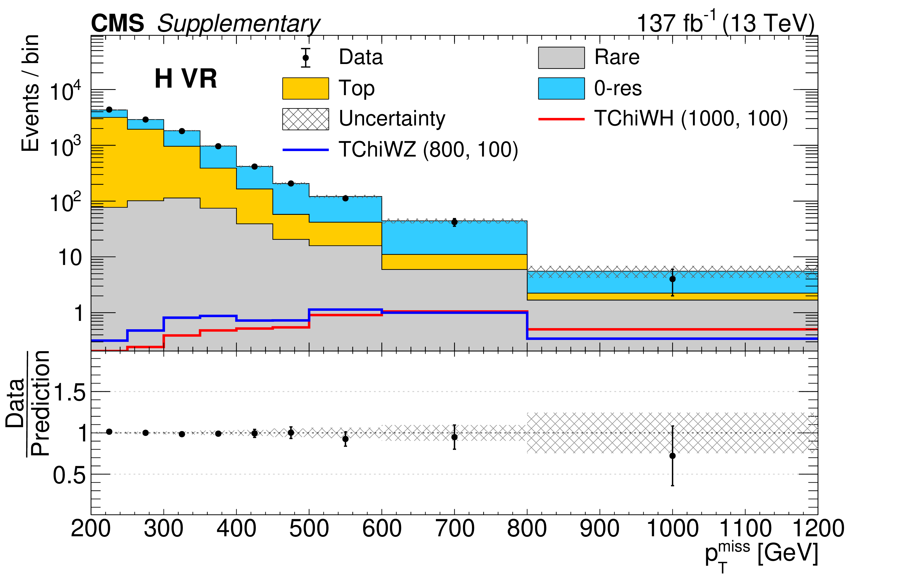
Additional Figure 10:
Data yields in the W (a) and H (b) b-tag validation regions compared to the predicted SM backgrounds as functions of $ p_{\mathrm{T}}^\text{miss} $. In these regions, events are required to pass the baseline selection except for the second AK8 jet requirement. Events are required to contain exactly one AK8 jet and at least one b-tagged AK4 jet. The hatched gray bands correspond to the total uncertainty in the prediction. The open histograms show the expectations from selected signal models, which are denoted in the legend by the name of the model followed by the assumed masses of the NLSP and LSP. |

png pdf |
Additional Figure 10-a:
Data yields in the W (a) and H (b) b-tag validation regions compared to the predicted SM backgrounds as functions of $ p_{\mathrm{T}}^\text{miss} $. In these regions, events are required to pass the baseline selection except for the second AK8 jet requirement. Events are required to contain exactly one AK8 jet and at least one b-tagged AK4 jet. The hatched gray bands correspond to the total uncertainty in the prediction. The open histograms show the expectations from selected signal models, which are denoted in the legend by the name of the model followed by the assumed masses of the NLSP and LSP. |
png pdf |
Additional Figure 10-b:
Data yields in the W (a) and H (b) b-tag validation regions compared to the predicted SM backgrounds as functions of $ p_{\mathrm{T}}^\text{miss} $. In these regions, events are required to pass the baseline selection except for the second AK8 jet requirement. Events are required to contain exactly one AK8 jet and at least one b-tagged AK4 jet. The hatched gray bands correspond to the total uncertainty in the prediction. The open histograms show the expectations from selected signal models, which are denoted in the legend by the name of the model followed by the assumed masses of the NLSP and LSP. |
png pdf |
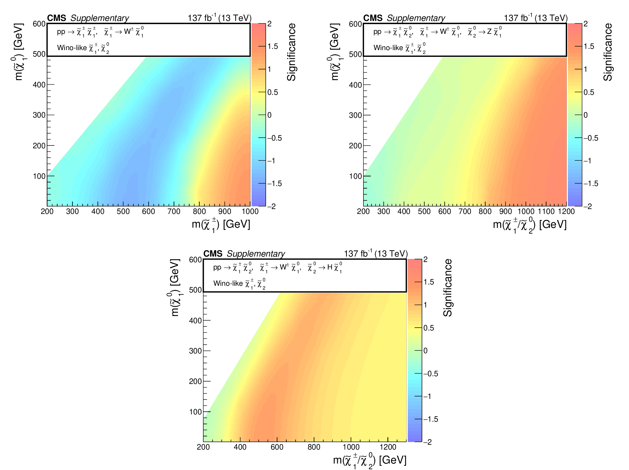
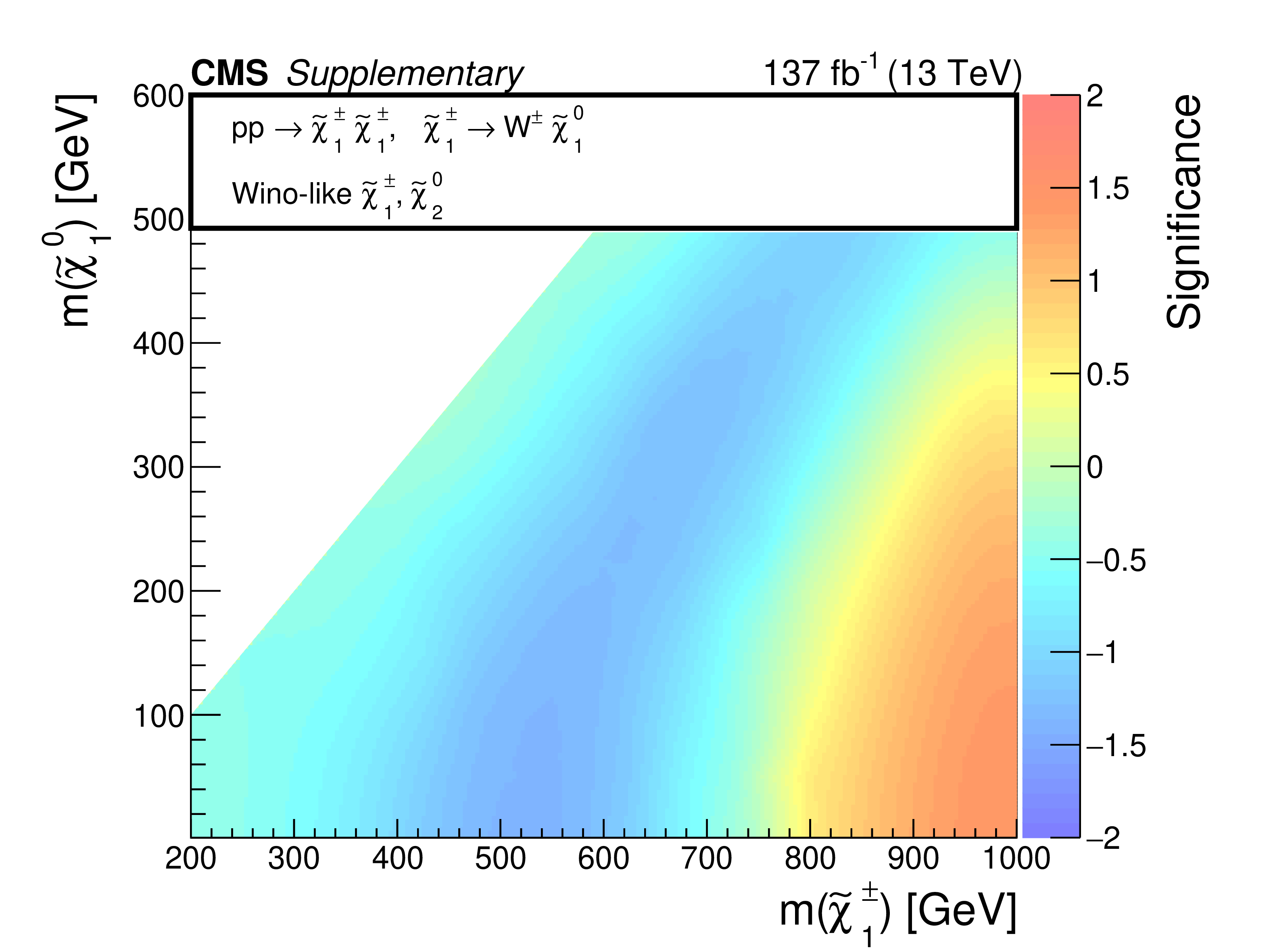
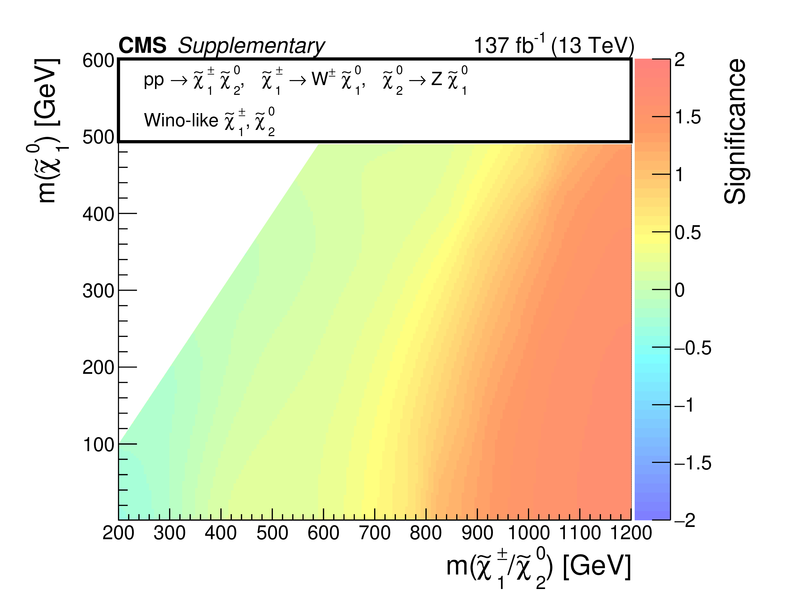
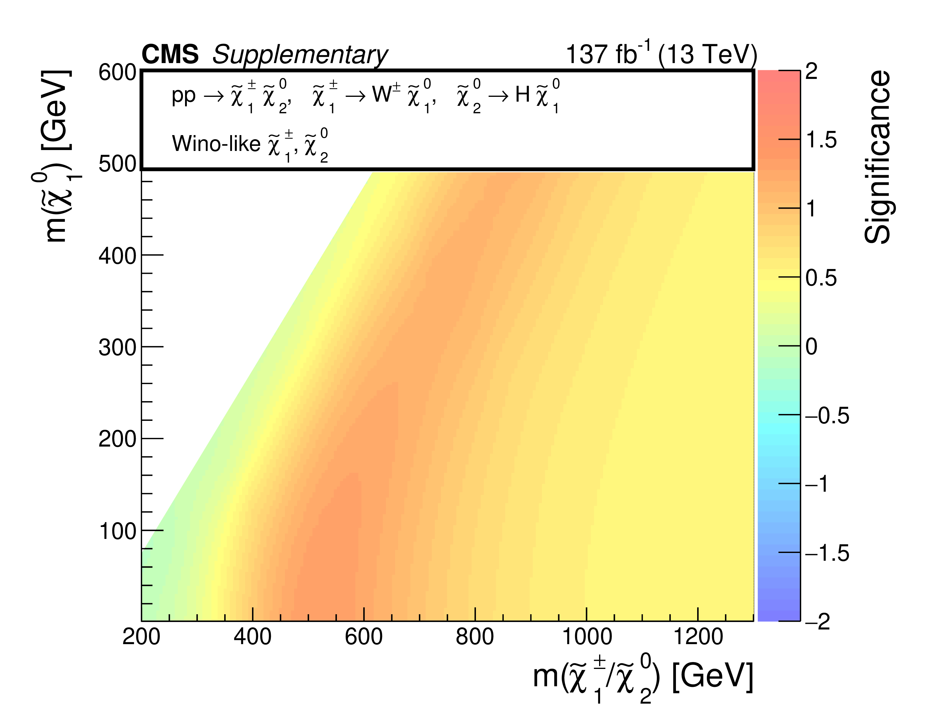
Additional Figure 11:
Observed significance of any excess in the data above the expected backgrounds, interpreted in the context of mass-degenerate wino-like $ \tilde{\chi}_{1}^{\pm}{\tilde{\chi}}{1}{\mp} $ production assuming $ \mathcal{B}(\tilde{\chi}_{1}^{\pm} \to \mathrm{W} \tilde{\chi}_{1}^{0})=100% $ for each $ \tilde{\chi}_{1}^{\pm} $ (a), as well as mass-degenerate wino-like $ \tilde{\chi}_{1}^{\pm}\tilde{\chi}_{2}^{0} $ production assuming $ \mathcal{B}(\tilde{\chi}_{1}^{\pm} \to \mathrm{W} \tilde{\chi}_{1}^{0})=100% $ and $ \mathcal{B}(\tilde{\chi}_{2}^{0} \to \mathrm{Z} \tilde{\chi}_{1}^{0})=100% $ (b) or $ \mathcal{B}(\tilde{\chi}_{2}^{0} \to \mathrm{H} \tilde{\chi}_{1}^{0})=100% $ (c). A negative significance indicates a data deficit below the expected backgrounds. |
png pdf |
Additional Figure 11-a:
Observed significance of any excess in the data above the expected backgrounds, interpreted in the context of mass-degenerate wino-like $ \tilde{\chi}_{1}^{\pm}{\tilde{\chi}}{1}{\mp} $ production assuming $ \mathcal{B}(\tilde{\chi}_{1}^{\pm} \to \mathrm{W} \tilde{\chi}_{1}^{0})=100% $ for each $ \tilde{\chi}_{1}^{\pm} $ (a), as well as mass-degenerate wino-like $ \tilde{\chi}_{1}^{\pm}\tilde{\chi}_{2}^{0} $ production assuming $ \mathcal{B}(\tilde{\chi}_{1}^{\pm} \to \mathrm{W} \tilde{\chi}_{1}^{0})=100% $ and $ \mathcal{B}(\tilde{\chi}_{2}^{0} \to \mathrm{Z} \tilde{\chi}_{1}^{0})=100% $ (b) or $ \mathcal{B}(\tilde{\chi}_{2}^{0} \to \mathrm{H} \tilde{\chi}_{1}^{0})=100% $ (c). A negative significance indicates a data deficit below the expected backgrounds. |
png pdf |
Additional Figure 11-b:
Observed significance of any excess in the data above the expected backgrounds, interpreted in the context of mass-degenerate wino-like $ \tilde{\chi}_{1}^{\pm}{\tilde{\chi}}{1}{\mp} $ production assuming $ \mathcal{B}(\tilde{\chi}_{1}^{\pm} \to \mathrm{W} \tilde{\chi}_{1}^{0})=100% $ for each $ \tilde{\chi}_{1}^{\pm} $ (a), as well as mass-degenerate wino-like $ \tilde{\chi}_{1}^{\pm}\tilde{\chi}_{2}^{0} $ production assuming $ \mathcal{B}(\tilde{\chi}_{1}^{\pm} \to \mathrm{W} \tilde{\chi}_{1}^{0})=100% $ and $ \mathcal{B}(\tilde{\chi}_{2}^{0} \to \mathrm{Z} \tilde{\chi}_{1}^{0})=100% $ (b) or $ \mathcal{B}(\tilde{\chi}_{2}^{0} \to \mathrm{H} \tilde{\chi}_{1}^{0})=100% $ (c). A negative significance indicates a data deficit below the expected backgrounds. |
png pdf |
Additional Figure 11-c:
Observed significance of any excess in the data above the expected backgrounds, interpreted in the context of mass-degenerate wino-like $ \tilde{\chi}_{1}^{\pm}{\tilde{\chi}}{1}{\mp} $ production assuming $ \mathcal{B}(\tilde{\chi}_{1}^{\pm} \to \mathrm{W} \tilde{\chi}_{1}^{0})=100% $ for each $ \tilde{\chi}_{1}^{\pm} $ (a), as well as mass-degenerate wino-like $ \tilde{\chi}_{1}^{\pm}\tilde{\chi}_{2}^{0} $ production assuming $ \mathcal{B}(\tilde{\chi}_{1}^{\pm} \to \mathrm{W} \tilde{\chi}_{1}^{0})=100% $ and $ \mathcal{B}(\tilde{\chi}_{2}^{0} \to \mathrm{Z} \tilde{\chi}_{1}^{0})=100% $ (b) or $ \mathcal{B}(\tilde{\chi}_{2}^{0} \to \mathrm{H} \tilde{\chi}_{1}^{0})=100% $ (c). A negative significance indicates a data deficit below the expected backgrounds. |
png pdf |
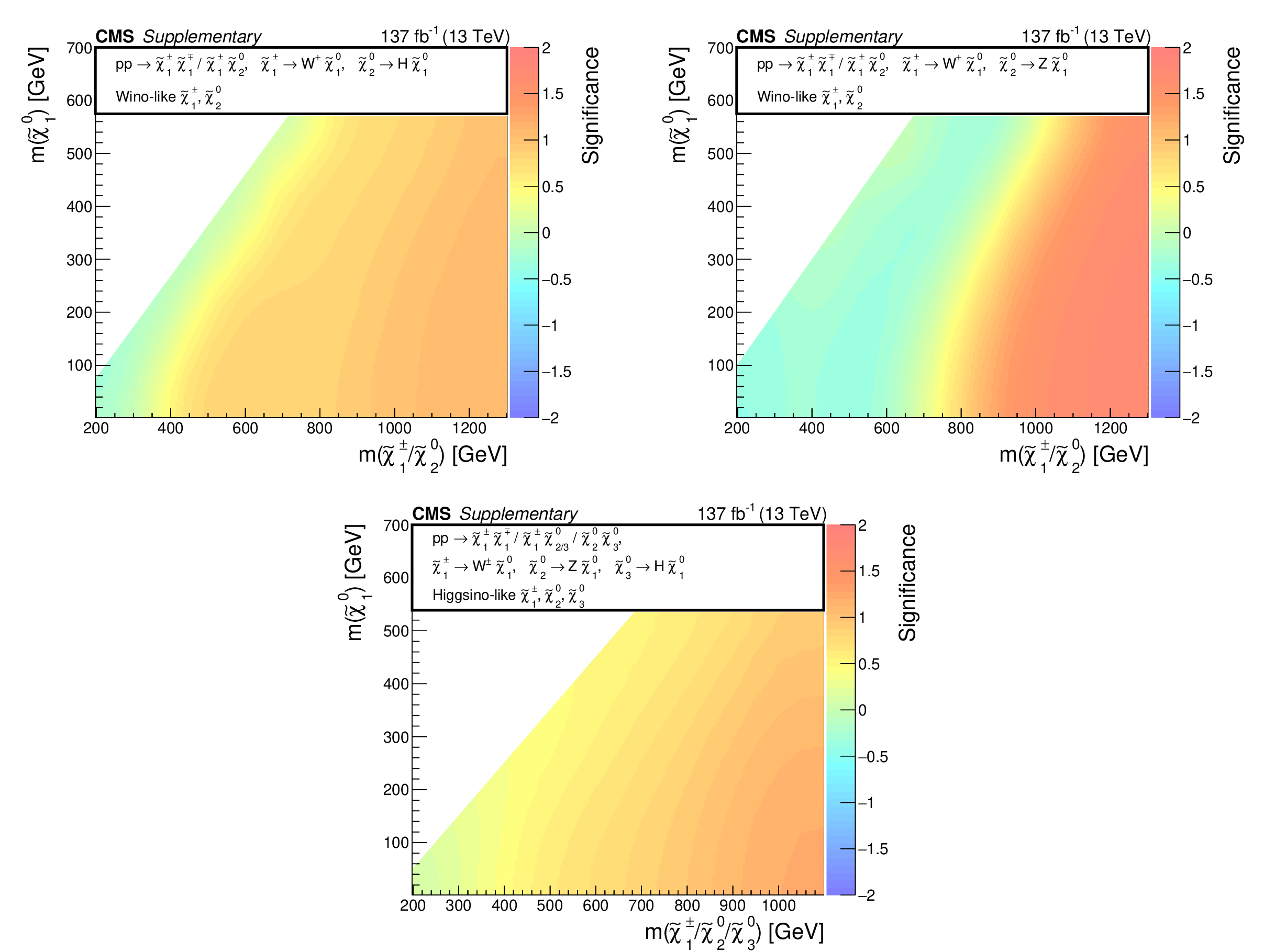
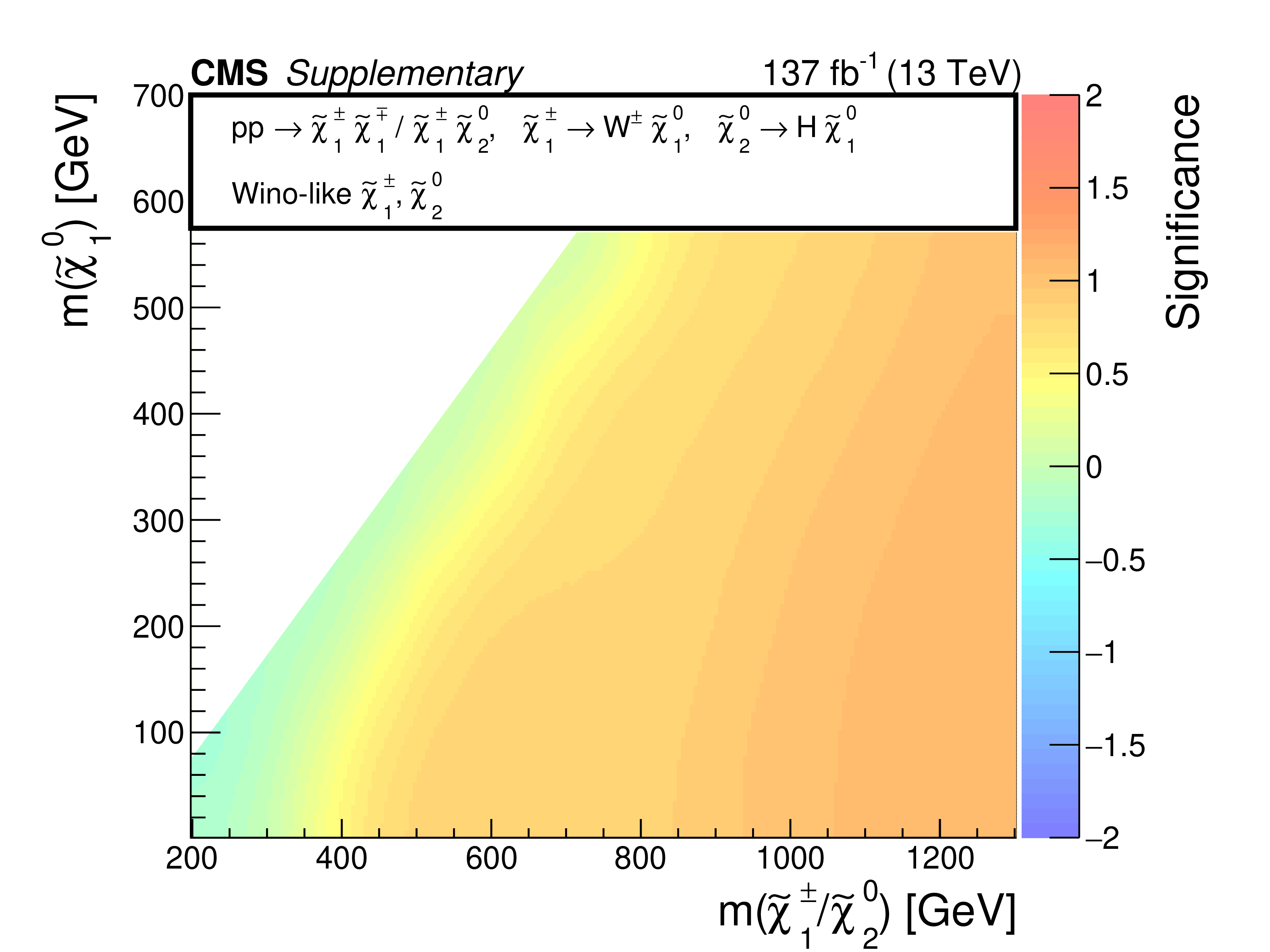
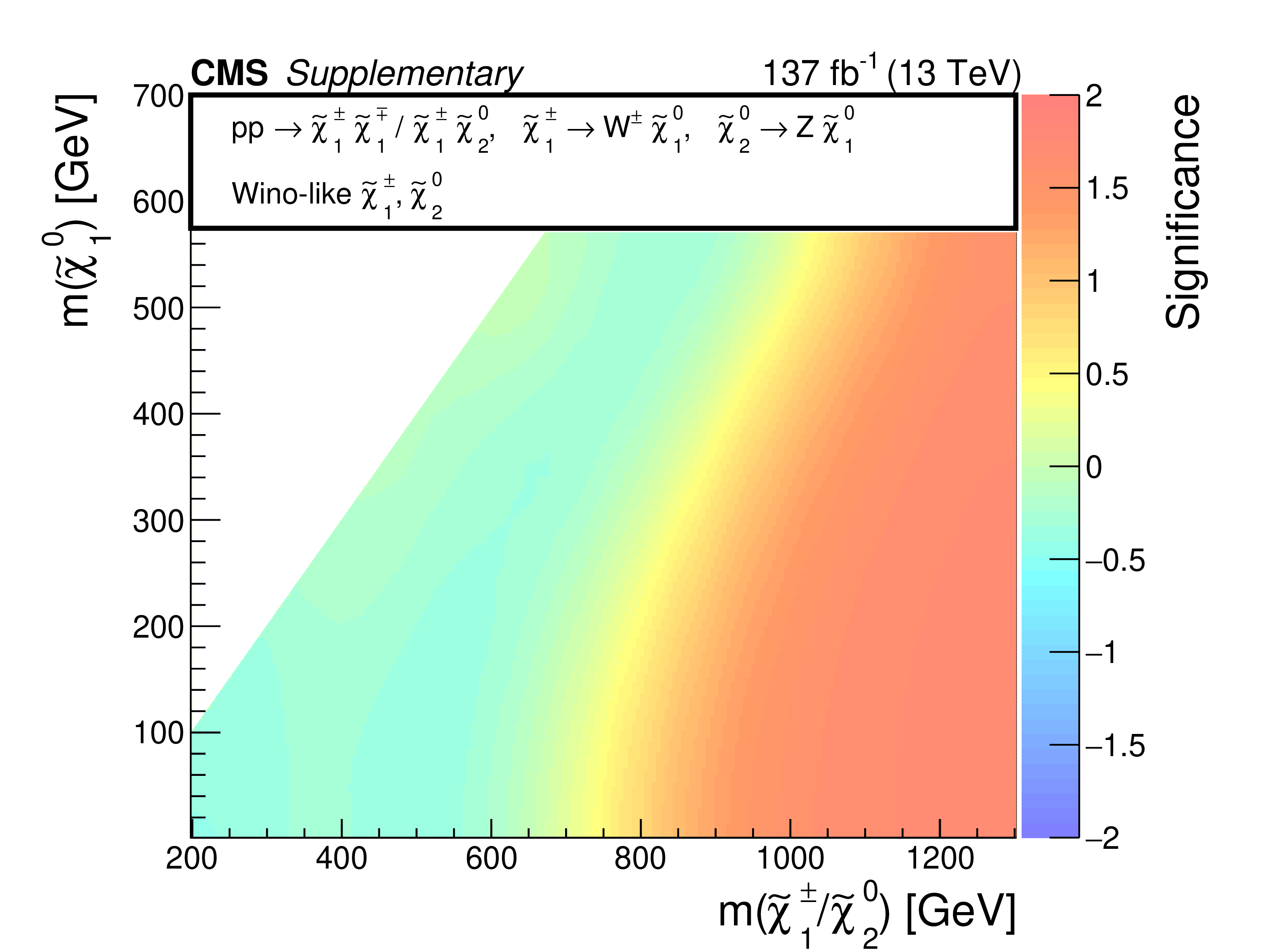
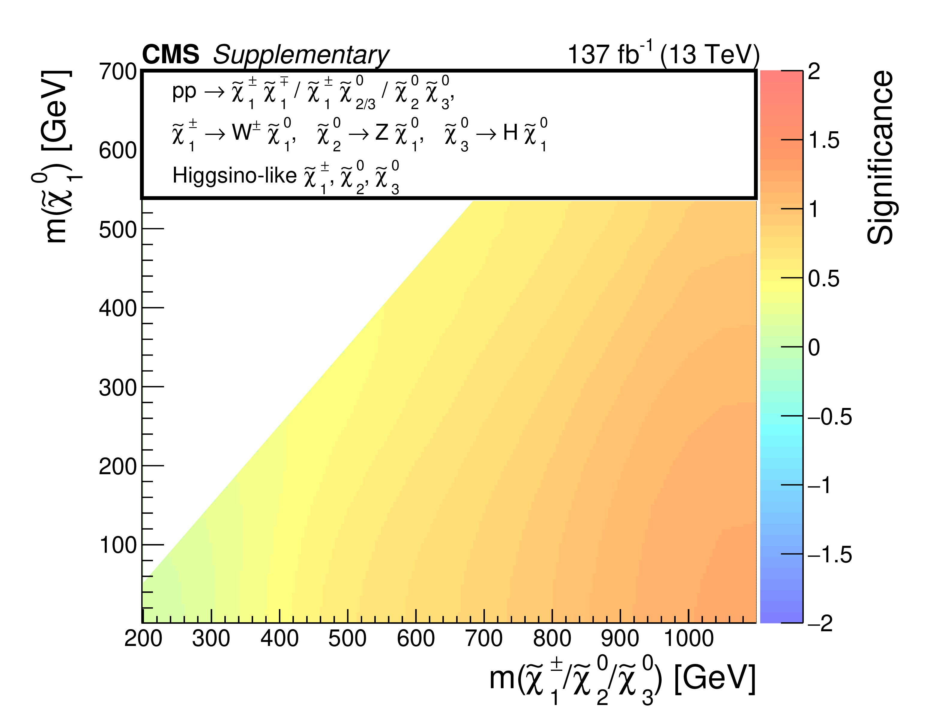
Additional Figure 12:
Observed significance of any excess in the data above the expected backgrounds, interpreted in the context of mass-degenerate wino-like $ \tilde{\chi}_{1}^{\pm}{\tilde{\chi}}{1}{\mp} $ and $ \tilde{\chi}_{1}^{\pm}\tilde{\chi}_{2}^{0} $ production assuming $ \mathcal{B}(\tilde{\chi}_{1}^{\pm} \to \mathrm{W} \tilde{\chi}_{1}^{0})=100% $ and $ \mathcal{B}(\tilde{\chi}_{2}^{0} \to \mathrm{H} \tilde{\chi}_{1}^{0})=100% $ (a) or $ \mathcal{B}(\tilde{\chi}_{2}^{0} \to \mathrm{Z} \tilde{\chi}_{1}^{0})=100% $ (b) and higgsino-like $ \tilde{\chi}_{1}^{\pm}\tilde{\chi}_{2}^{0} $, $ \tilde{\chi}_{1}^{\pm}\tilde{\chi}_{3}^{0} $, $ \tilde{\chi}_{1}^{\pm}{\tilde{\chi}}{1}{\mp} $, and $ \tilde{\chi}_{2}^{0}\tilde{\chi}_{3}^{0} $ production assuming $ \mathcal{B}(\tilde{\chi}_{1}^{\pm} \to \mathrm{W} \tilde{\chi}_{1}^{0})=100% $, $ \mathcal{B}(\tilde{\chi}_{2}^{0} \to \mathrm{Z} \tilde{\chi}_{1}^{0})=100% $, and $ \mathcal{B}(\tilde{\chi}_{3}^{0} \to \mathrm{H} \tilde{\chi}_{1}^{0})=100% $ (c) as functions of the NLSP and LSP masses. A negative significance indicates a data deficit below the expected backgrounds. |
png pdf |
Additional Figure 12-a:
Observed significance of any excess in the data above the expected backgrounds, interpreted in the context of mass-degenerate wino-like $ \tilde{\chi}_{1}^{\pm}{\tilde{\chi}}{1}{\mp} $ and $ \tilde{\chi}_{1}^{\pm}\tilde{\chi}_{2}^{0} $ production assuming $ \mathcal{B}(\tilde{\chi}_{1}^{\pm} \to \mathrm{W} \tilde{\chi}_{1}^{0})=100% $ and $ \mathcal{B}(\tilde{\chi}_{2}^{0} \to \mathrm{H} \tilde{\chi}_{1}^{0})=100% $ (a) or $ \mathcal{B}(\tilde{\chi}_{2}^{0} \to \mathrm{Z} \tilde{\chi}_{1}^{0})=100% $ (b) and higgsino-like $ \tilde{\chi}_{1}^{\pm}\tilde{\chi}_{2}^{0} $, $ \tilde{\chi}_{1}^{\pm}\tilde{\chi}_{3}^{0} $, $ \tilde{\chi}_{1}^{\pm}{\tilde{\chi}}{1}{\mp} $, and $ \tilde{\chi}_{2}^{0}\tilde{\chi}_{3}^{0} $ production assuming $ \mathcal{B}(\tilde{\chi}_{1}^{\pm} \to \mathrm{W} \tilde{\chi}_{1}^{0})=100% $, $ \mathcal{B}(\tilde{\chi}_{2}^{0} \to \mathrm{Z} \tilde{\chi}_{1}^{0})=100% $, and $ \mathcal{B}(\tilde{\chi}_{3}^{0} \to \mathrm{H} \tilde{\chi}_{1}^{0})=100% $ (c) as functions of the NLSP and LSP masses. A negative significance indicates a data deficit below the expected backgrounds. |
png pdf |
Additional Figure 12-b:
Observed significance of any excess in the data above the expected backgrounds, interpreted in the context of mass-degenerate wino-like $ \tilde{\chi}_{1}^{\pm}{\tilde{\chi}}{1}{\mp} $ and $ \tilde{\chi}_{1}^{\pm}\tilde{\chi}_{2}^{0} $ production assuming $ \mathcal{B}(\tilde{\chi}_{1}^{\pm} \to \mathrm{W} \tilde{\chi}_{1}^{0})=100% $ and $ \mathcal{B}(\tilde{\chi}_{2}^{0} \to \mathrm{H} \tilde{\chi}_{1}^{0})=100% $ (a) or $ \mathcal{B}(\tilde{\chi}_{2}^{0} \to \mathrm{Z} \tilde{\chi}_{1}^{0})=100% $ (b) and higgsino-like $ \tilde{\chi}_{1}^{\pm}\tilde{\chi}_{2}^{0} $, $ \tilde{\chi}_{1}^{\pm}\tilde{\chi}_{3}^{0} $, $ \tilde{\chi}_{1}^{\pm}{\tilde{\chi}}{1}{\mp} $, and $ \tilde{\chi}_{2}^{0}\tilde{\chi}_{3}^{0} $ production assuming $ \mathcal{B}(\tilde{\chi}_{1}^{\pm} \to \mathrm{W} \tilde{\chi}_{1}^{0})=100% $, $ \mathcal{B}(\tilde{\chi}_{2}^{0} \to \mathrm{Z} \tilde{\chi}_{1}^{0})=100% $, and $ \mathcal{B}(\tilde{\chi}_{3}^{0} \to \mathrm{H} \tilde{\chi}_{1}^{0})=100% $ (c) as functions of the NLSP and LSP masses. A negative significance indicates a data deficit below the expected backgrounds. |
png pdf |
Additional Figure 12-c:
Observed significance of any excess in the data above the expected backgrounds, interpreted in the context of mass-degenerate wino-like $ \tilde{\chi}_{1}^{\pm}{\tilde{\chi}}{1}{\mp} $ and $ \tilde{\chi}_{1}^{\pm}\tilde{\chi}_{2}^{0} $ production assuming $ \mathcal{B}(\tilde{\chi}_{1}^{\pm} \to \mathrm{W} \tilde{\chi}_{1}^{0})=100% $ and $ \mathcal{B}(\tilde{\chi}_{2}^{0} \to \mathrm{H} \tilde{\chi}_{1}^{0})=100% $ (a) or $ \mathcal{B}(\tilde{\chi}_{2}^{0} \to \mathrm{Z} \tilde{\chi}_{1}^{0})=100% $ (b) and higgsino-like $ \tilde{\chi}_{1}^{\pm}\tilde{\chi}_{2}^{0} $, $ \tilde{\chi}_{1}^{\pm}\tilde{\chi}_{3}^{0} $, $ \tilde{\chi}_{1}^{\pm}{\tilde{\chi}}{1}{\mp} $, and $ \tilde{\chi}_{2}^{0}\tilde{\chi}_{3}^{0} $ production assuming $ \mathcal{B}(\tilde{\chi}_{1}^{\pm} \to \mathrm{W} \tilde{\chi}_{1}^{0})=100% $, $ \mathcal{B}(\tilde{\chi}_{2}^{0} \to \mathrm{Z} \tilde{\chi}_{1}^{0})=100% $, and $ \mathcal{B}(\tilde{\chi}_{3}^{0} \to \mathrm{H} \tilde{\chi}_{1}^{0})=100% $ (c) as functions of the NLSP and LSP masses. A negative significance indicates a data deficit below the expected backgrounds. |

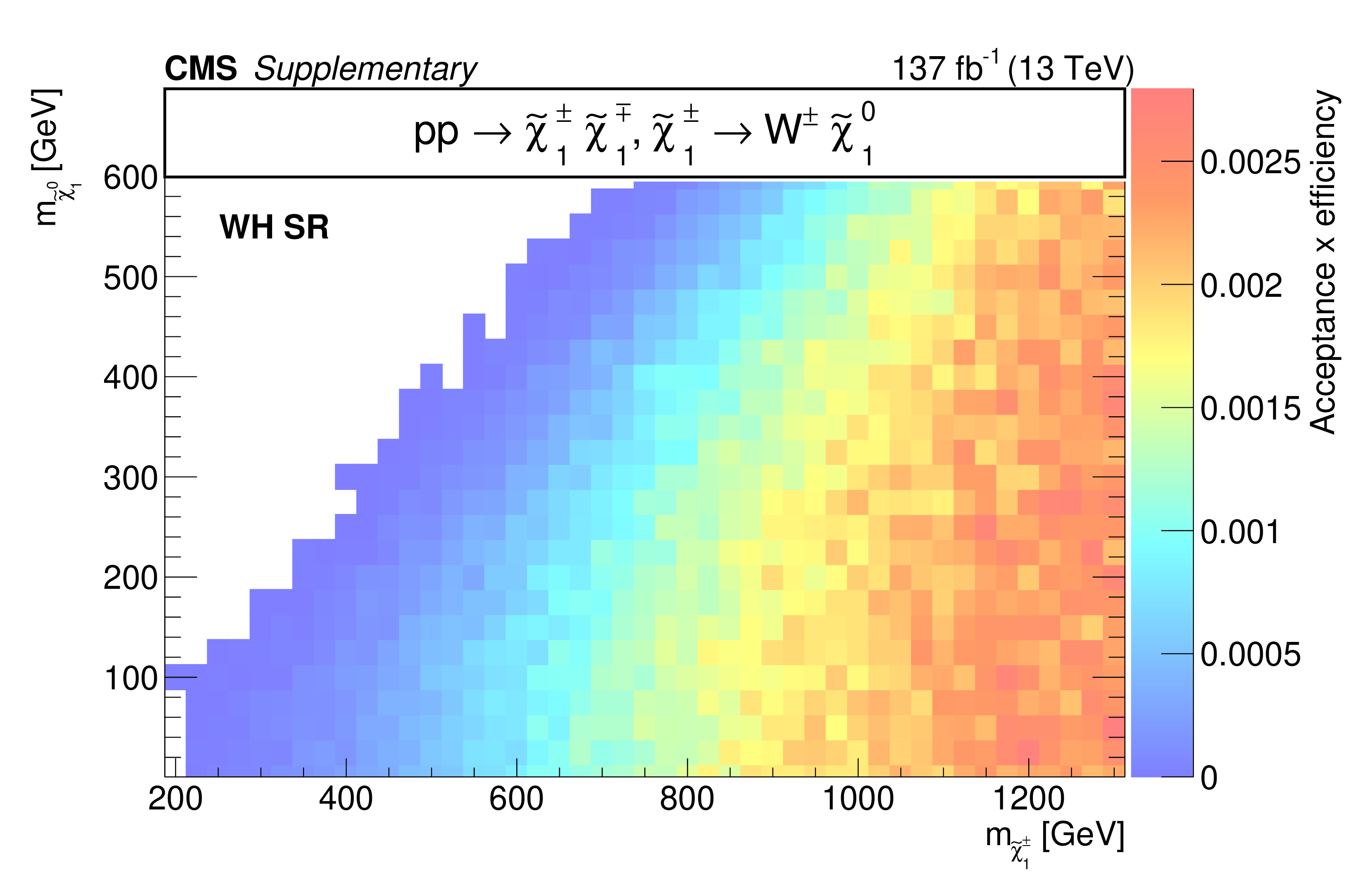
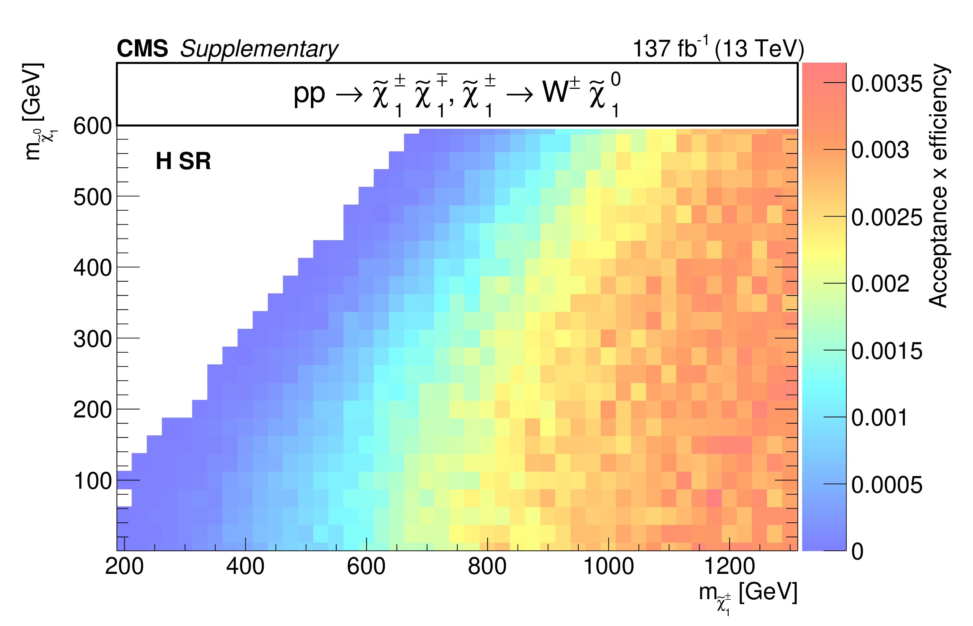
png pdf root |
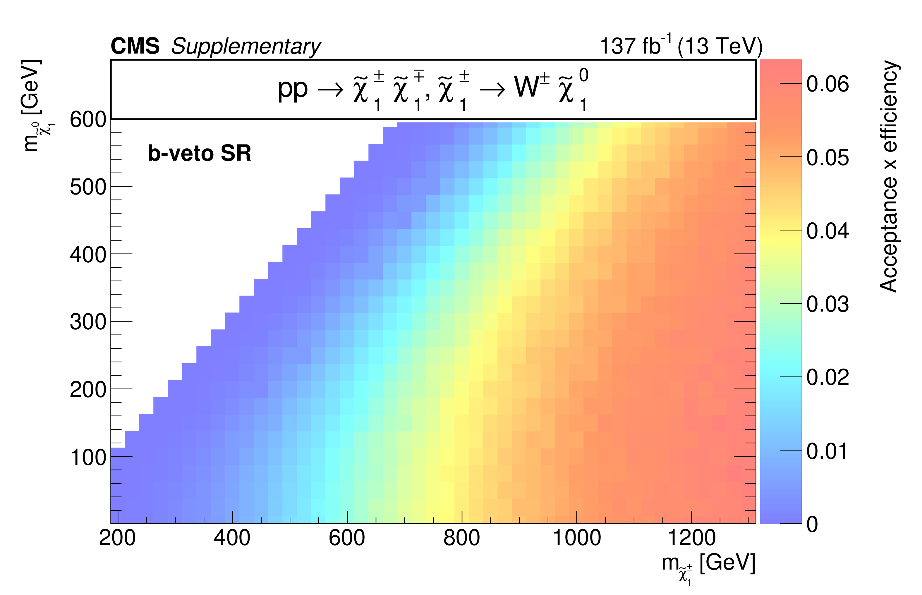
Additional Figure 13:
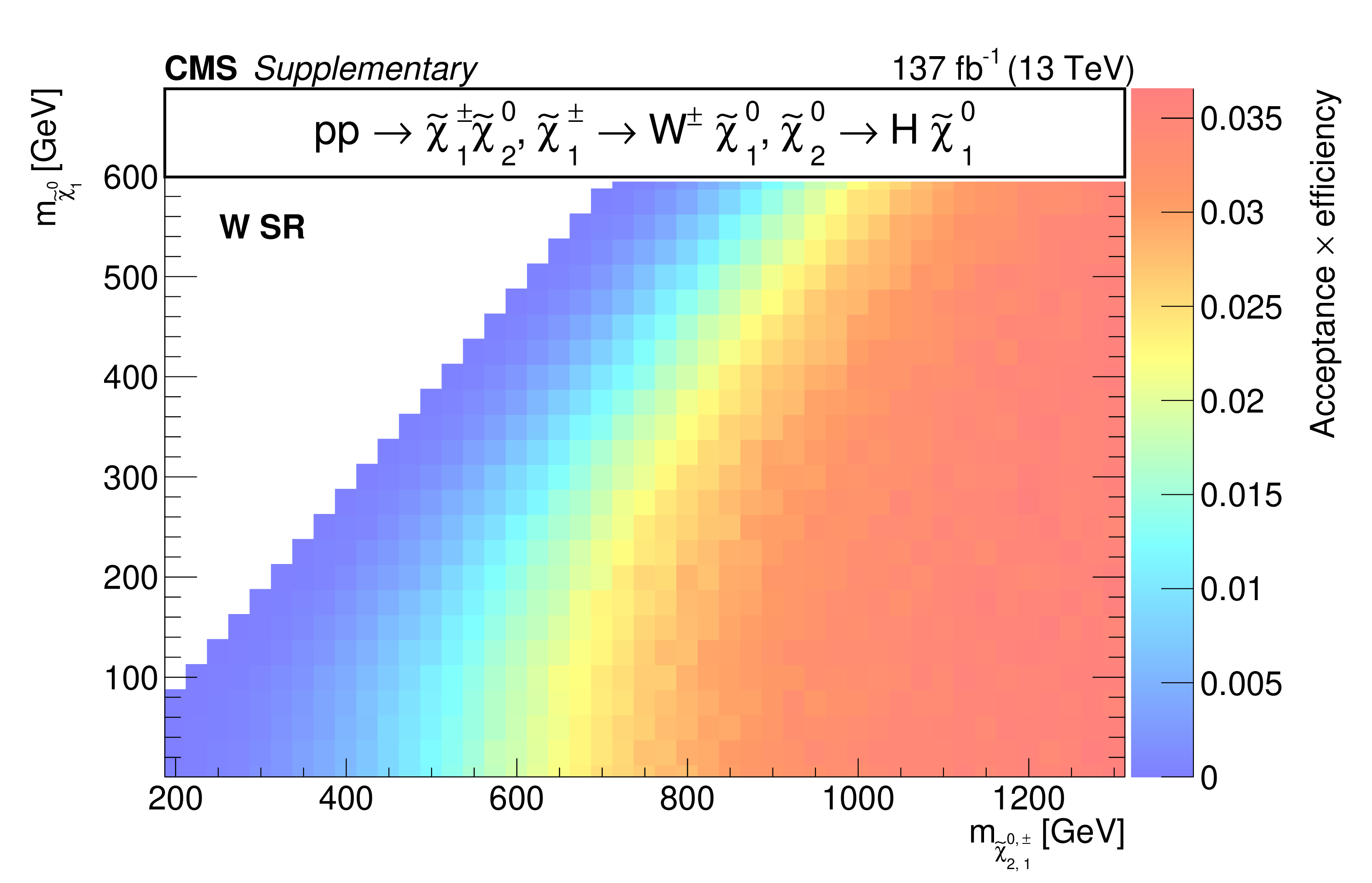
Acceptance times efficiency ($ A\epsilon $) for the TChiWW model in the b-veto SR (a), WH SR (b), W SR (c), and H SR (d). |
png pdf root |
Additional Figure 13-a:
Acceptance times efficiency ($ A\epsilon $) for the TChiWW model in the b-veto SR (a), WH SR (b), W SR (c), and H SR (d). |
png pdf root |
Additional Figure 13-b:
Acceptance times efficiency ($ A\epsilon $) for the TChiWW model in the b-veto SR (a), WH SR (b), W SR (c), and H SR (d). |

png pdf root |
Additional Figure 13-c:
Acceptance times efficiency ($ A\epsilon $) for the TChiWW model in the b-veto SR (a), WH SR (b), W SR (c), and H SR (d). |
png pdf root |
Additional Figure 13-d:
Acceptance times efficiency ($ A\epsilon $) for the TChiWW model in the b-veto SR (a), WH SR (b), W SR (c), and H SR (d). |
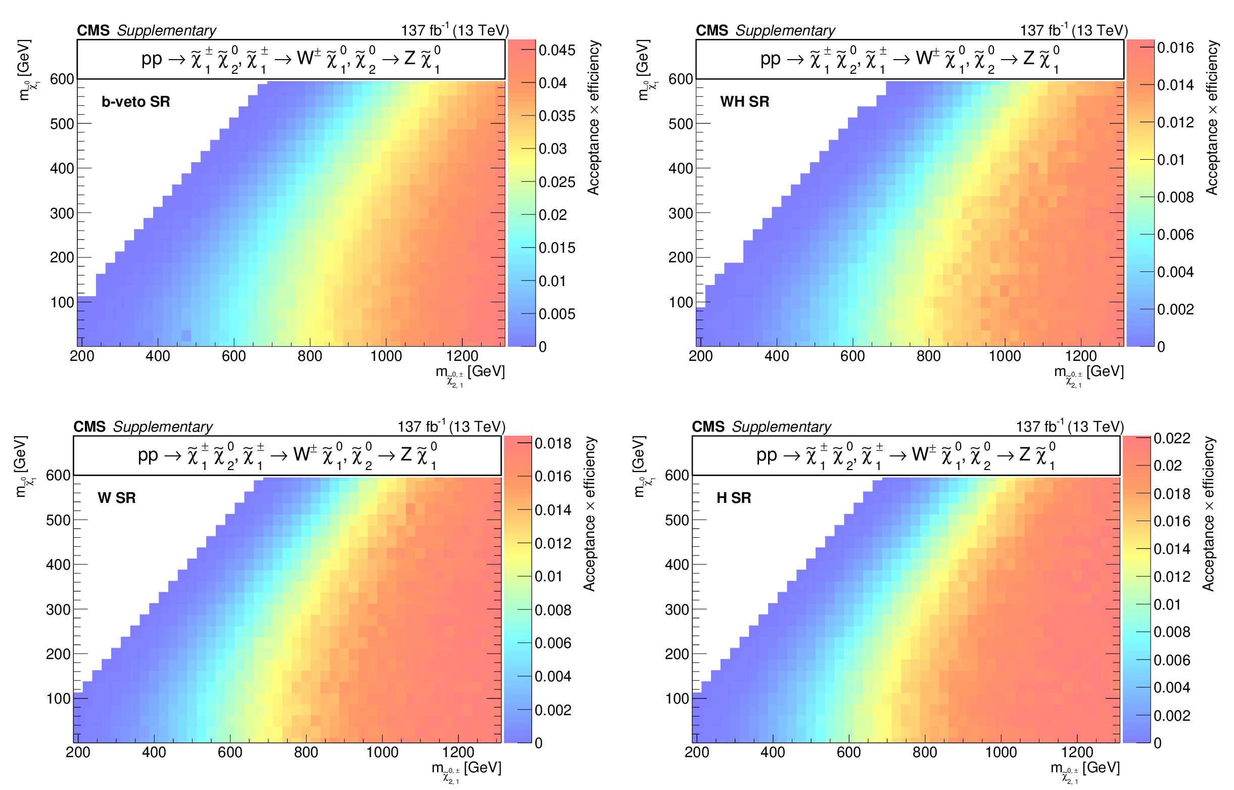
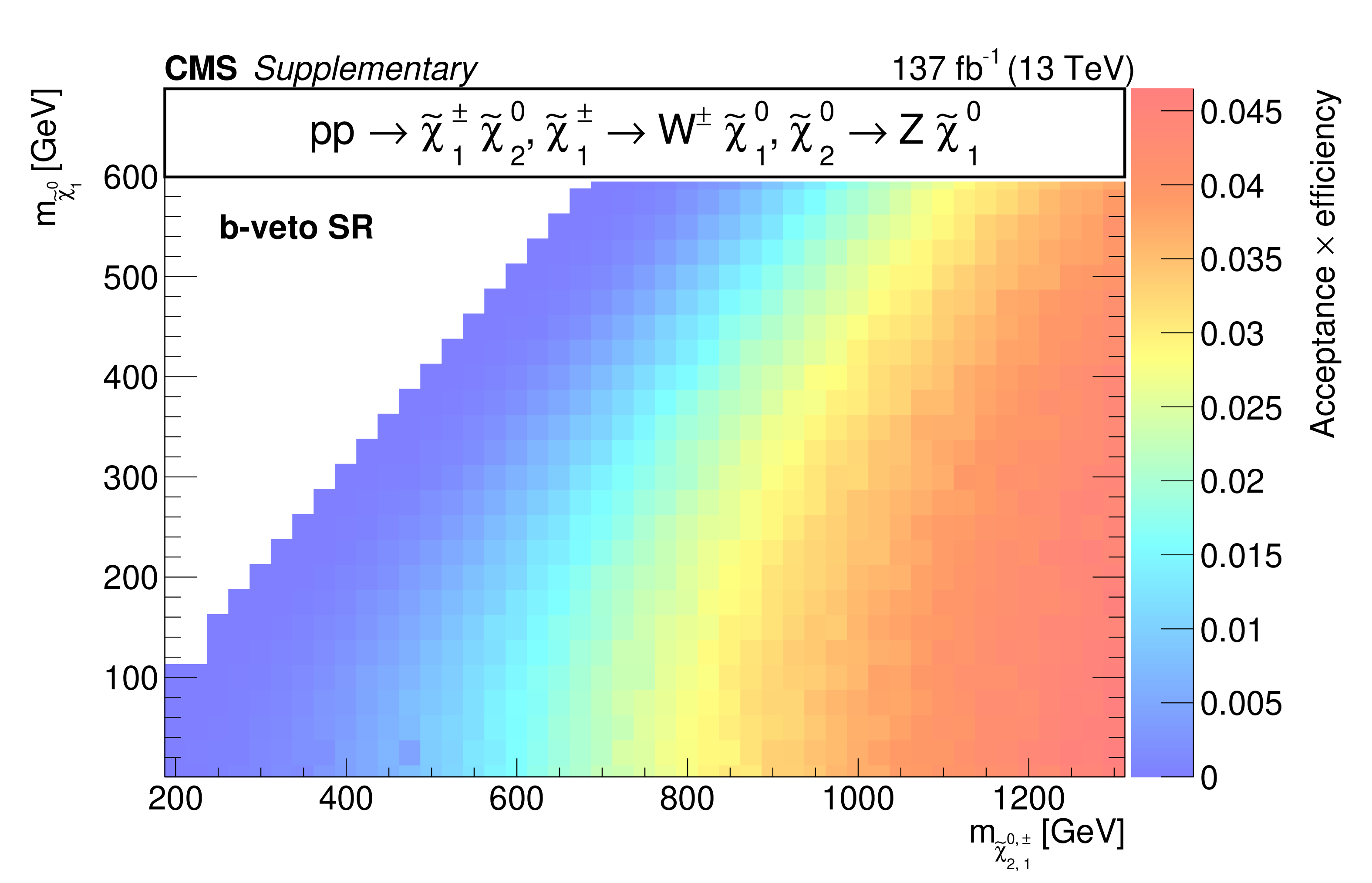
png pdf root |
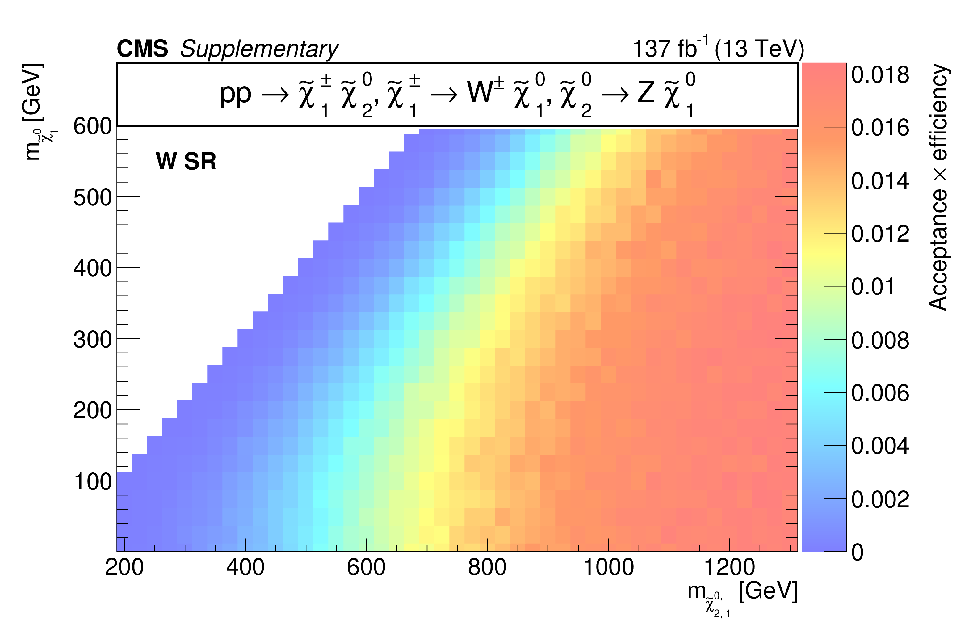
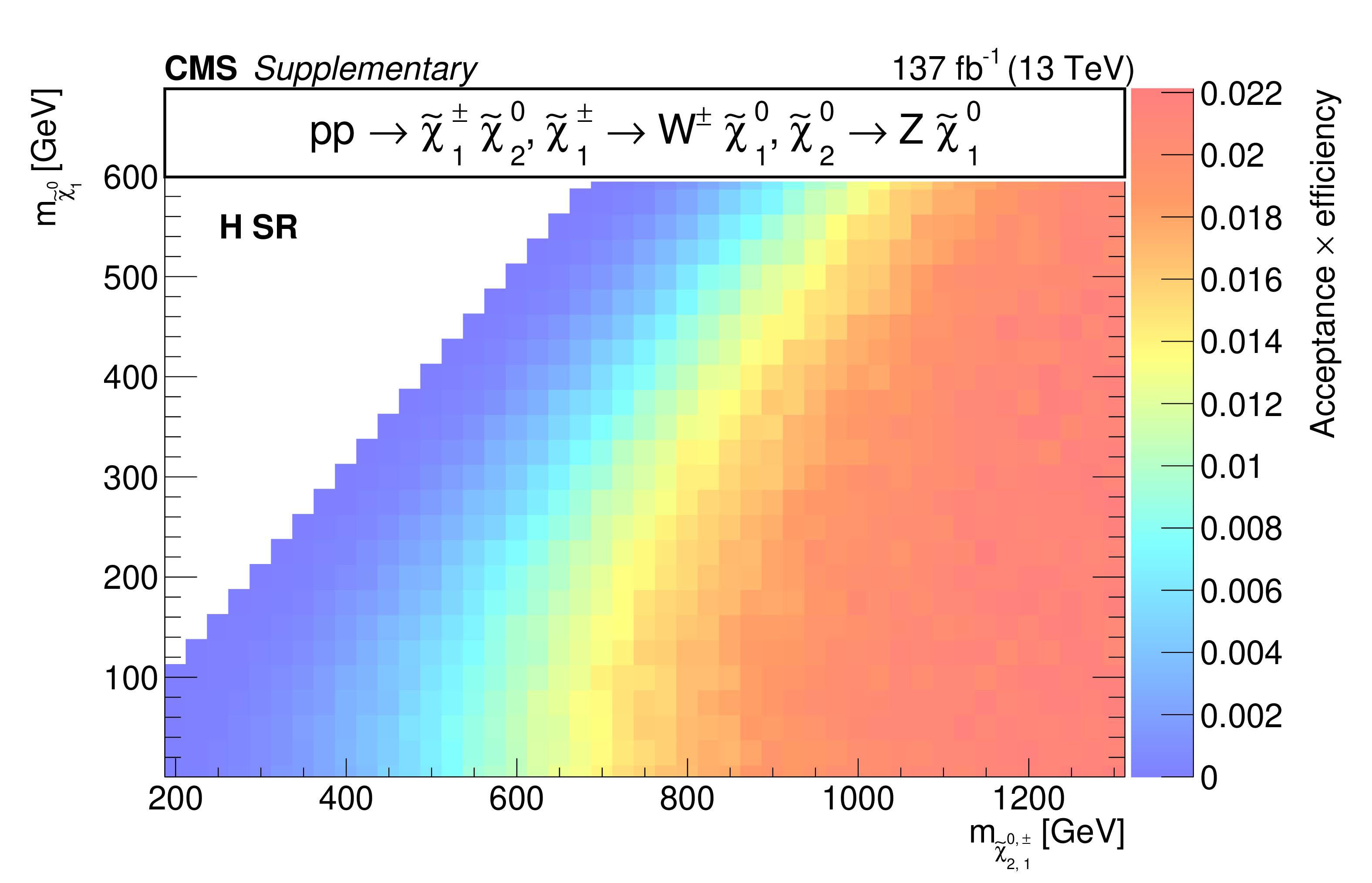
Additional Figure 14:
Acceptance times efficiency ($ A\epsilon $) for the TChiWZ model in the b-veto SR (a), WH SR (b), W SR (c), and H SR (d). |
png pdf root |
Additional Figure 14-a:
Acceptance times efficiency ($ A\epsilon $) for the TChiWZ model in the b-veto SR (a), WH SR (b), W SR (c), and H SR (d). |

png pdf root |
Additional Figure 14-b:
Acceptance times efficiency ($ A\epsilon $) for the TChiWZ model in the b-veto SR (a), WH SR (b), W SR (c), and H SR (d). |
png pdf root |
Additional Figure 14-c:
Acceptance times efficiency ($ A\epsilon $) for the TChiWZ model in the b-veto SR (a), WH SR (b), W SR (c), and H SR (d). |
png pdf root |
Additional Figure 14-d:
Acceptance times efficiency ($ A\epsilon $) for the TChiWZ model in the b-veto SR (a), WH SR (b), W SR (c), and H SR (d). |
png pdf root |
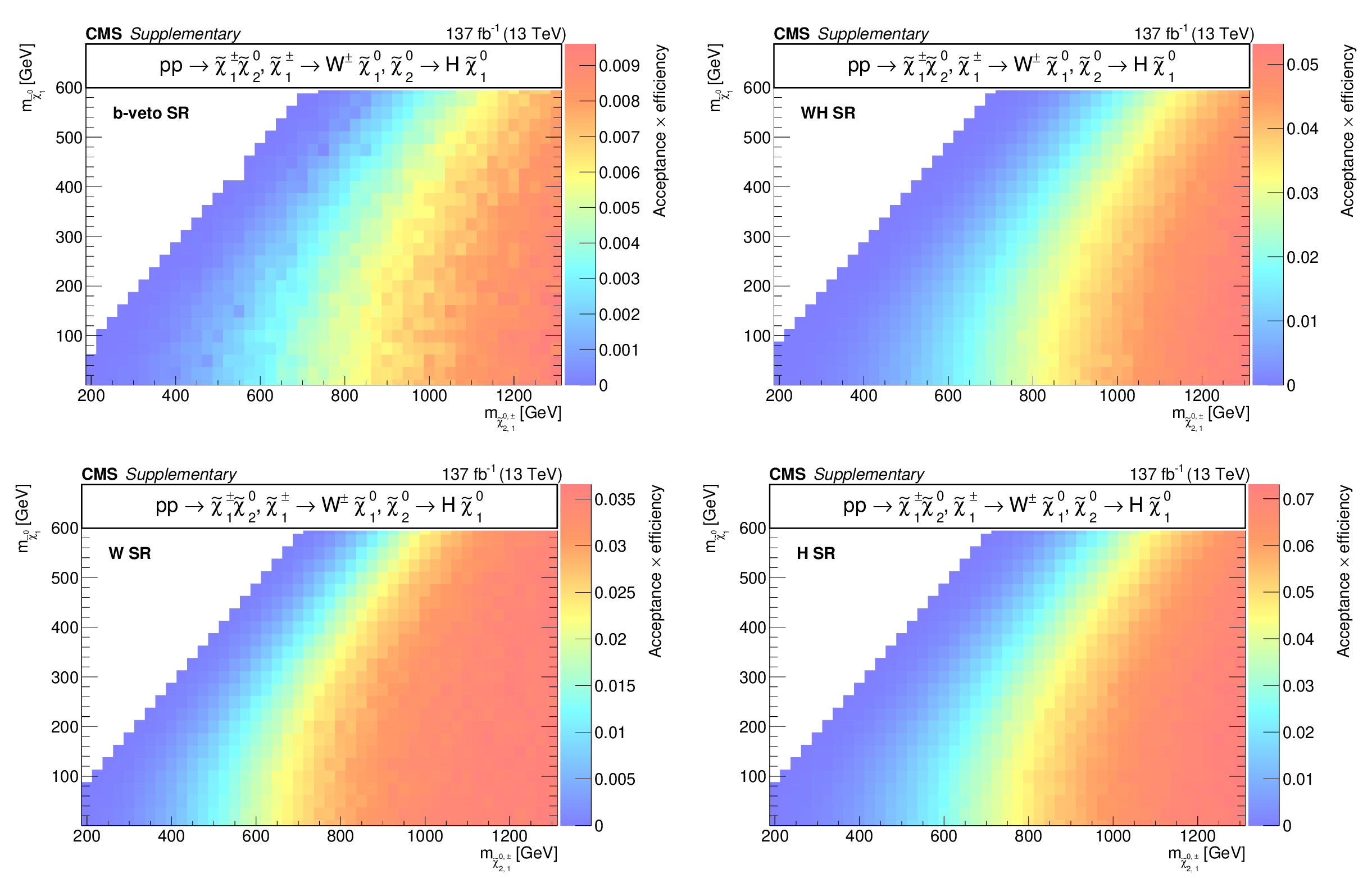
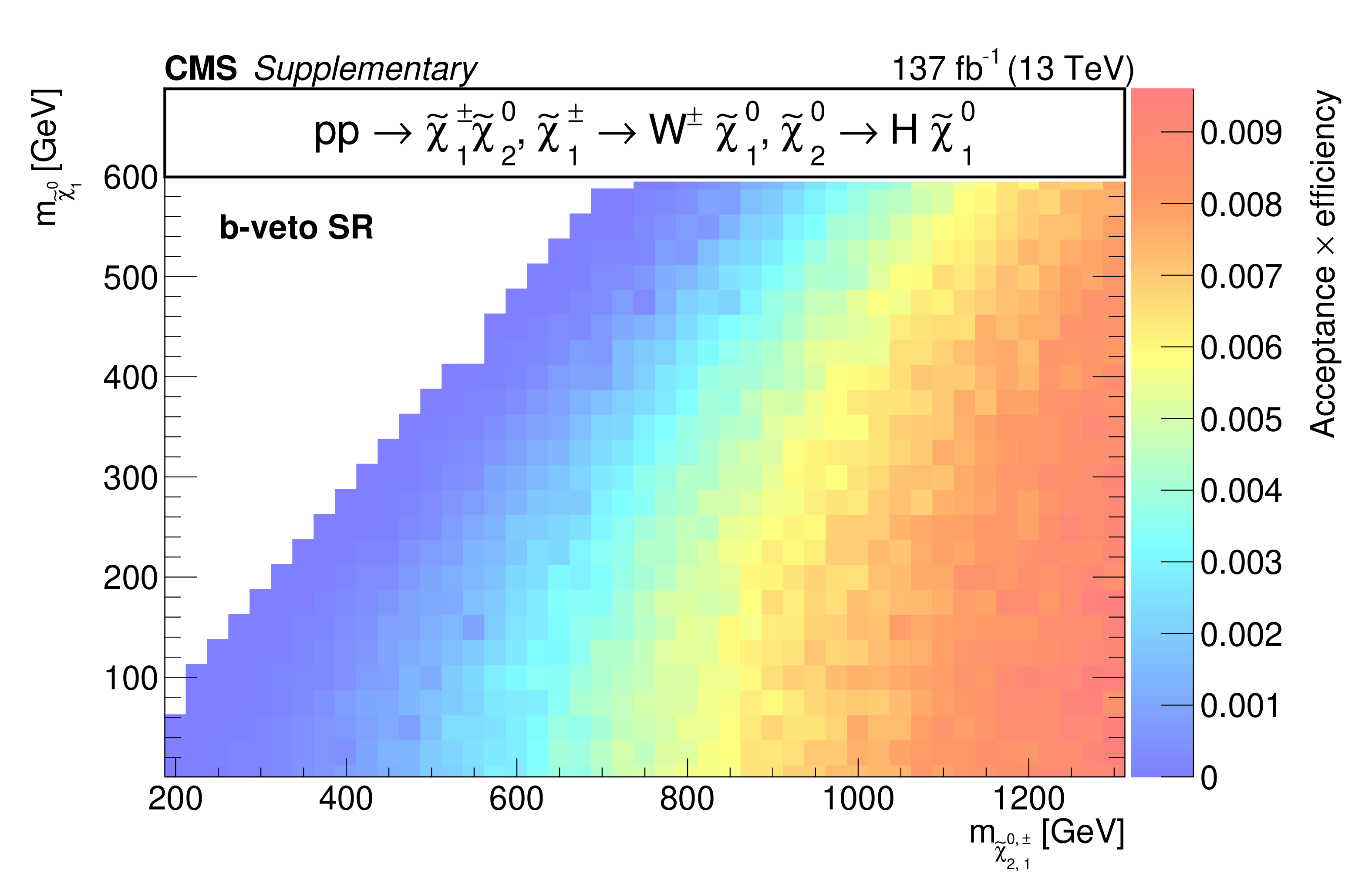
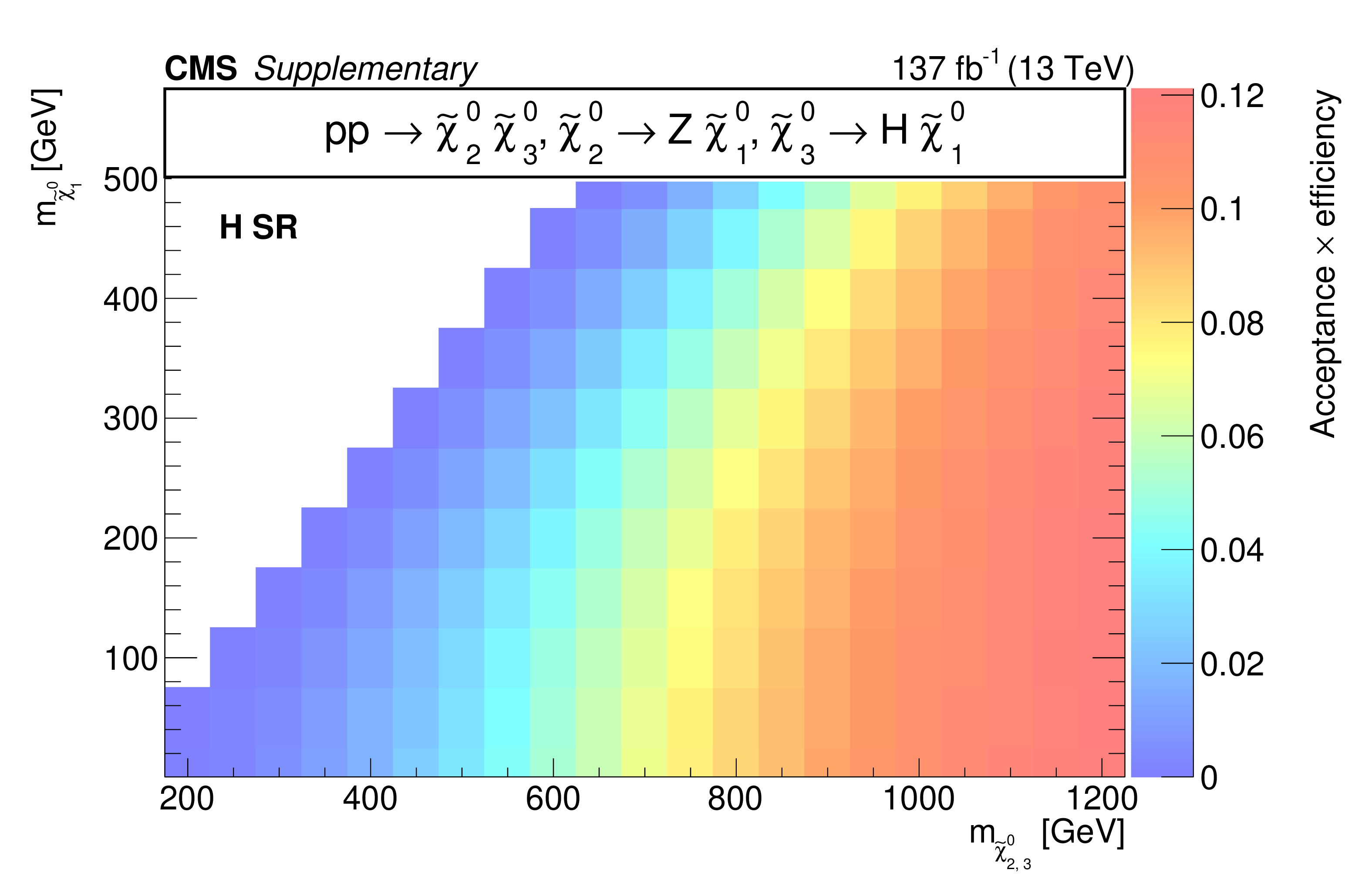
Additional Figure 15:
Acceptance times efficiency ($ A\epsilon $) for the TChiWH model in the b-veto SR (a), WH SR (b), W SR (c), and H SR (d). |
png pdf root |
Additional Figure 15-a:
Acceptance times efficiency ($ A\epsilon $) for the TChiWH model in the b-veto SR (a), WH SR (b), W SR (c), and H SR (d). |

png pdf root |
Additional Figure 15-b:
Acceptance times efficiency ($ A\epsilon $) for the TChiWH model in the b-veto SR (a), WH SR (b), W SR (c), and H SR (d). |
png pdf root |
Additional Figure 15-c:
Acceptance times efficiency ($ A\epsilon $) for the TChiWH model in the b-veto SR (a), WH SR (b), W SR (c), and H SR (d). |

png pdf root |
Additional Figure 15-d:
Acceptance times efficiency ($ A\epsilon $) for the TChiWH model in the b-veto SR (a), WH SR (b), W SR (c), and H SR (d). |
png pdf root |
Additional Figure 16:
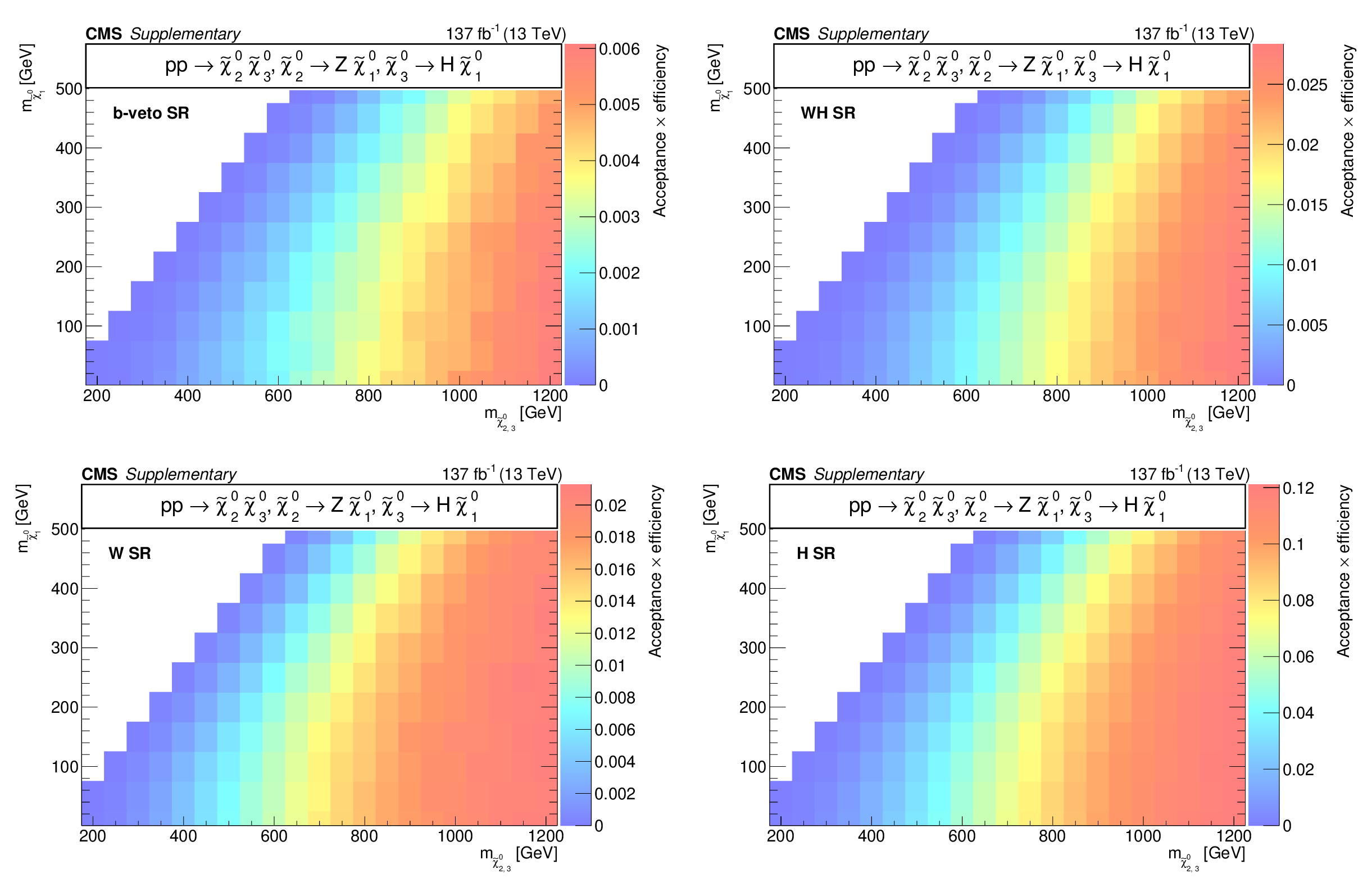
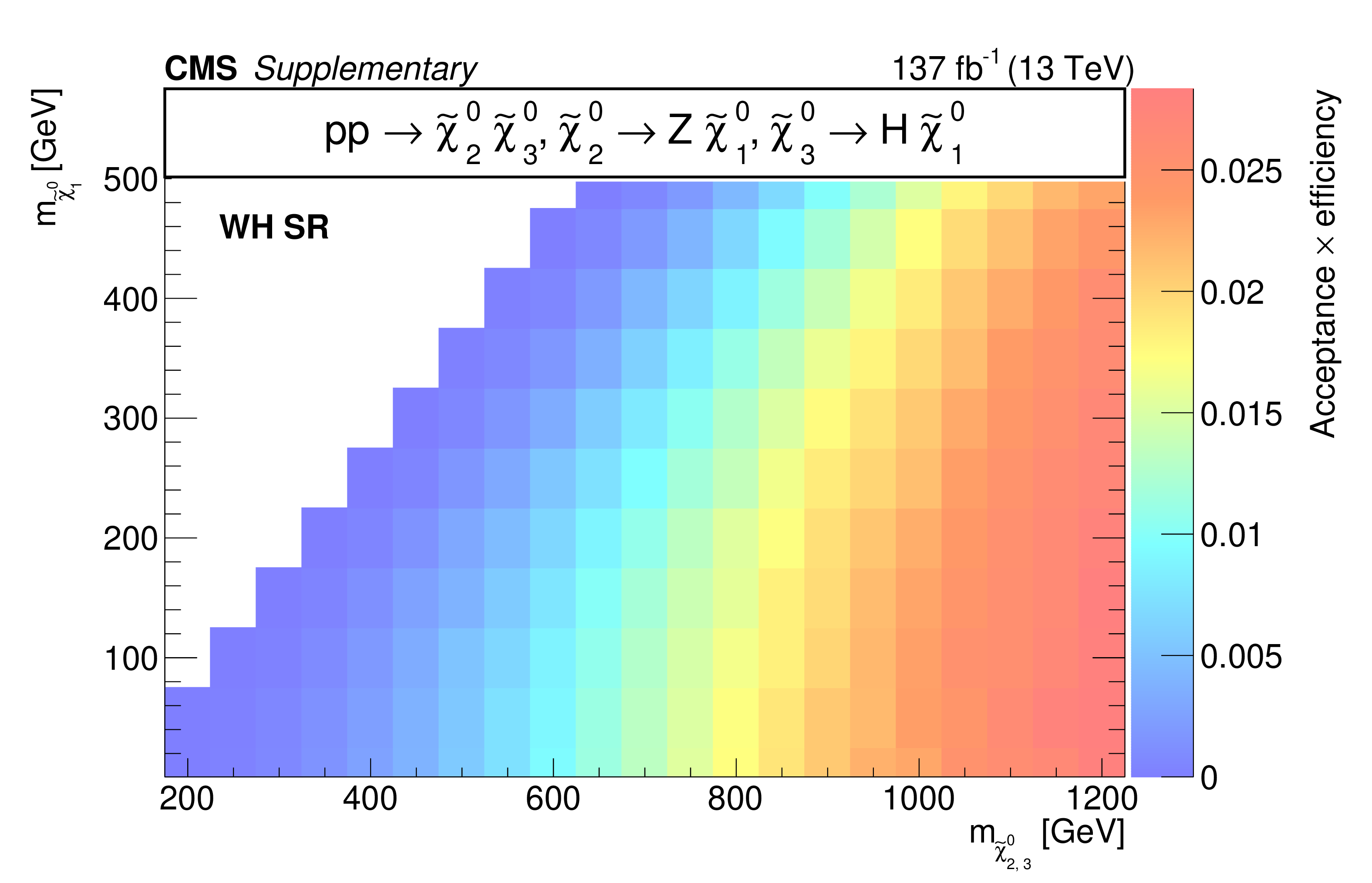
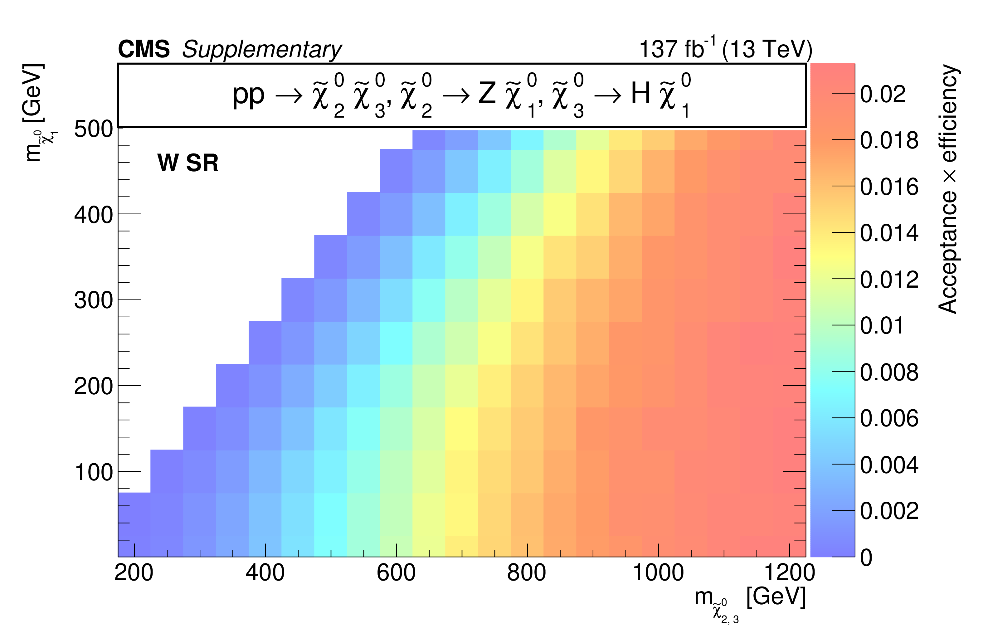
Acceptance times efficiency ($ A\epsilon $) for the TChiHZ model in the b-veto SR (a), WH SR (b), W SR (c), and H SR (d). |

png pdf root |
Additional Figure 16-a:
Acceptance times efficiency ($ A\epsilon $) for the TChiHZ model in the b-veto SR (a), WH SR (b), W SR (c), and H SR (d). |
png pdf root |
Additional Figure 16-b:
Acceptance times efficiency ($ A\epsilon $) for the TChiHZ model in the b-veto SR (a), WH SR (b), W SR (c), and H SR (d). |
png pdf root |
Additional Figure 16-c:
Acceptance times efficiency ($ A\epsilon $) for the TChiHZ model in the b-veto SR (a), WH SR (b), W SR (c), and H SR (d). |
png pdf root |
Additional Figure 16-d:
Acceptance times efficiency ($ A\epsilon $) for the TChiHZ model in the b-veto SR (a), WH SR (b), W SR (c), and H SR (d). |
png pdf |
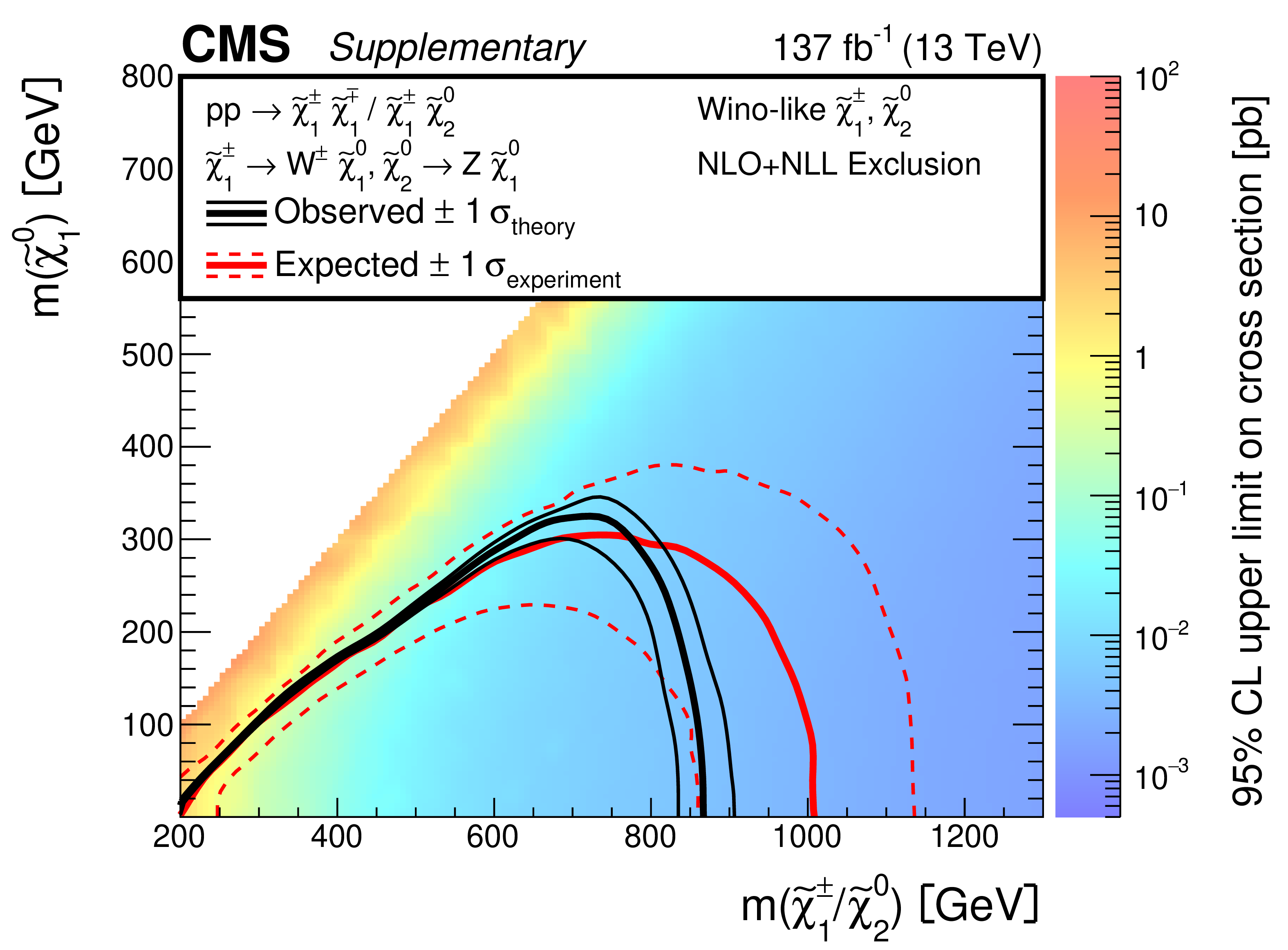
Additional Figure 17:
Expected and observed 95% CL upper limits on mass-degenerate wino-like $ \tilde{\chi}_{1}^{\pm}{\tilde{\chi}}{1}{\mp} $ and $ \tilde{\chi}_{1}^{\pm}\tilde{\chi}_{2}^{0} $ production, assuming $ \mathcal{B}(\tilde{\chi}_{1}^{\pm}\to\mathrm{W}\tilde{\chi}_{1}^{0}) = 100% $, and either $ \mathcal{B}(\tilde{\chi}_{2}^{0}\to\mathrm{Z}\tilde{\chi}_{1}^{0}) = 100% $ (a) or $ \mathcal{B}(\tilde{\chi}_{2}^{0}\to\mathrm{H}\tilde{\chi}_{1}^{0}) = 100% $ (b). In each of these two plots, the red (black) contours represent the expected (observed) mass exclusion limits. Mass exclusion limits are computed assuming wino-like cross sections. |
png pdf root |
Additional Figure 17-a:
Expected and observed 95% CL upper limits on mass-degenerate wino-like $ \tilde{\chi}_{1}^{\pm}{\tilde{\chi}}{1}{\mp} $ and $ \tilde{\chi}_{1}^{\pm}\tilde{\chi}_{2}^{0} $ production, assuming $ \mathcal{B}(\tilde{\chi}_{1}^{\pm}\to\mathrm{W}\tilde{\chi}_{1}^{0}) = 100% $, and either $ \mathcal{B}(\tilde{\chi}_{2}^{0}\to\mathrm{Z}\tilde{\chi}_{1}^{0}) = 100% $ (a) or $ \mathcal{B}(\tilde{\chi}_{2}^{0}\to\mathrm{H}\tilde{\chi}_{1}^{0}) = 100% $ (b). In each of these two plots, the red (black) contours represent the expected (observed) mass exclusion limits. Mass exclusion limits are computed assuming wino-like cross sections. |
png pdf root |
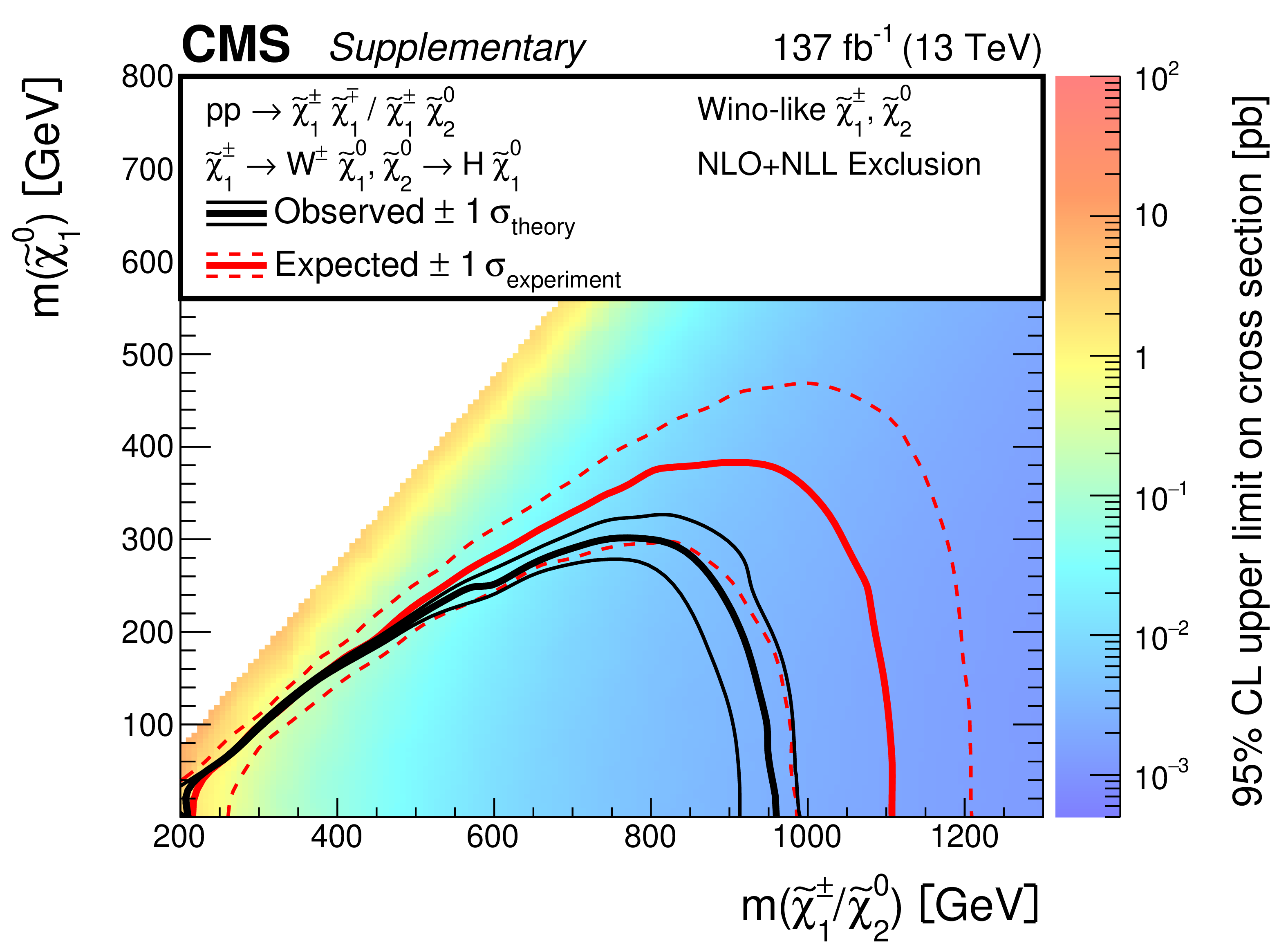
Additional Figure 17-b:
Expected and observed 95% CL upper limits on mass-degenerate wino-like $ \tilde{\chi}_{1}^{\pm}{\tilde{\chi}}{1}{\mp} $ and $ \tilde{\chi}_{1}^{\pm}\tilde{\chi}_{2}^{0} $ production, assuming $ \mathcal{B}(\tilde{\chi}_{1}^{\pm}\to\mathrm{W}\tilde{\chi}_{1}^{0}) = 100% $, and either $ \mathcal{B}(\tilde{\chi}_{2}^{0}\to\mathrm{Z}\tilde{\chi}_{1}^{0}) = 100% $ (a) or $ \mathcal{B}(\tilde{\chi}_{2}^{0}\to\mathrm{H}\tilde{\chi}_{1}^{0}) = 100% $ (b). In each of these two plots, the red (black) contours represent the expected (observed) mass exclusion limits. Mass exclusion limits are computed assuming wino-like cross sections. |
png pdf root |
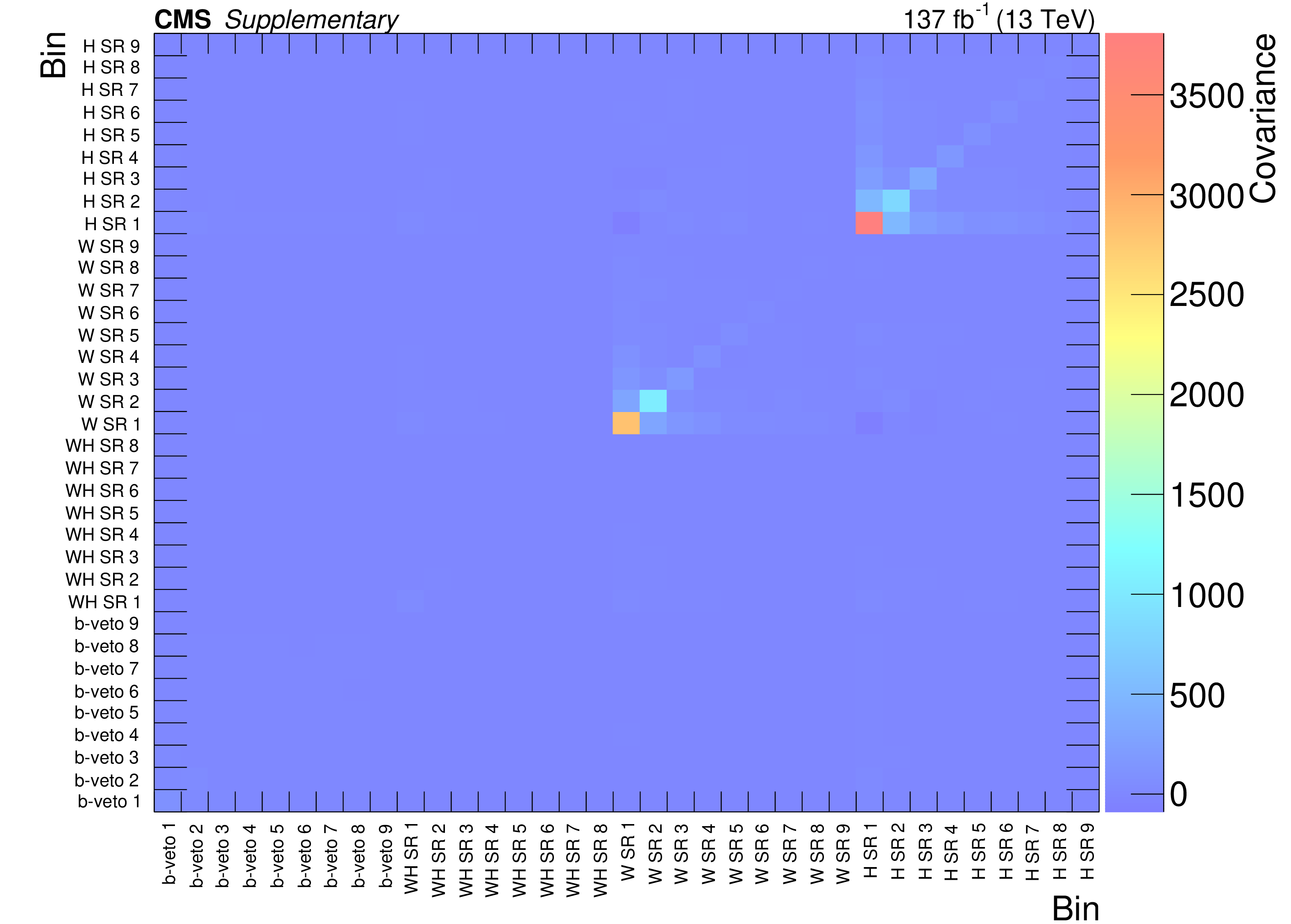
Additional Figure 18:
Covariance matrix for the signal regions, derived from a fit to the control regions only under the background-only hypothesis. |
png pdf root |
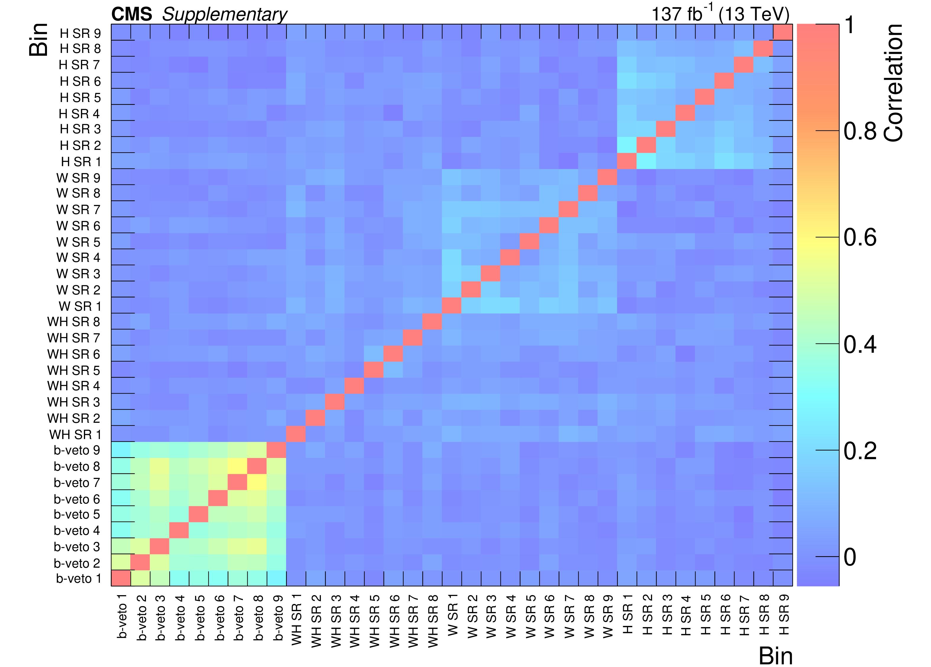
Additional Figure 19:
Correlation matrix for the signal regions, derived from a fit to the control regions only under the background-only hypothesis. |
png pdf |
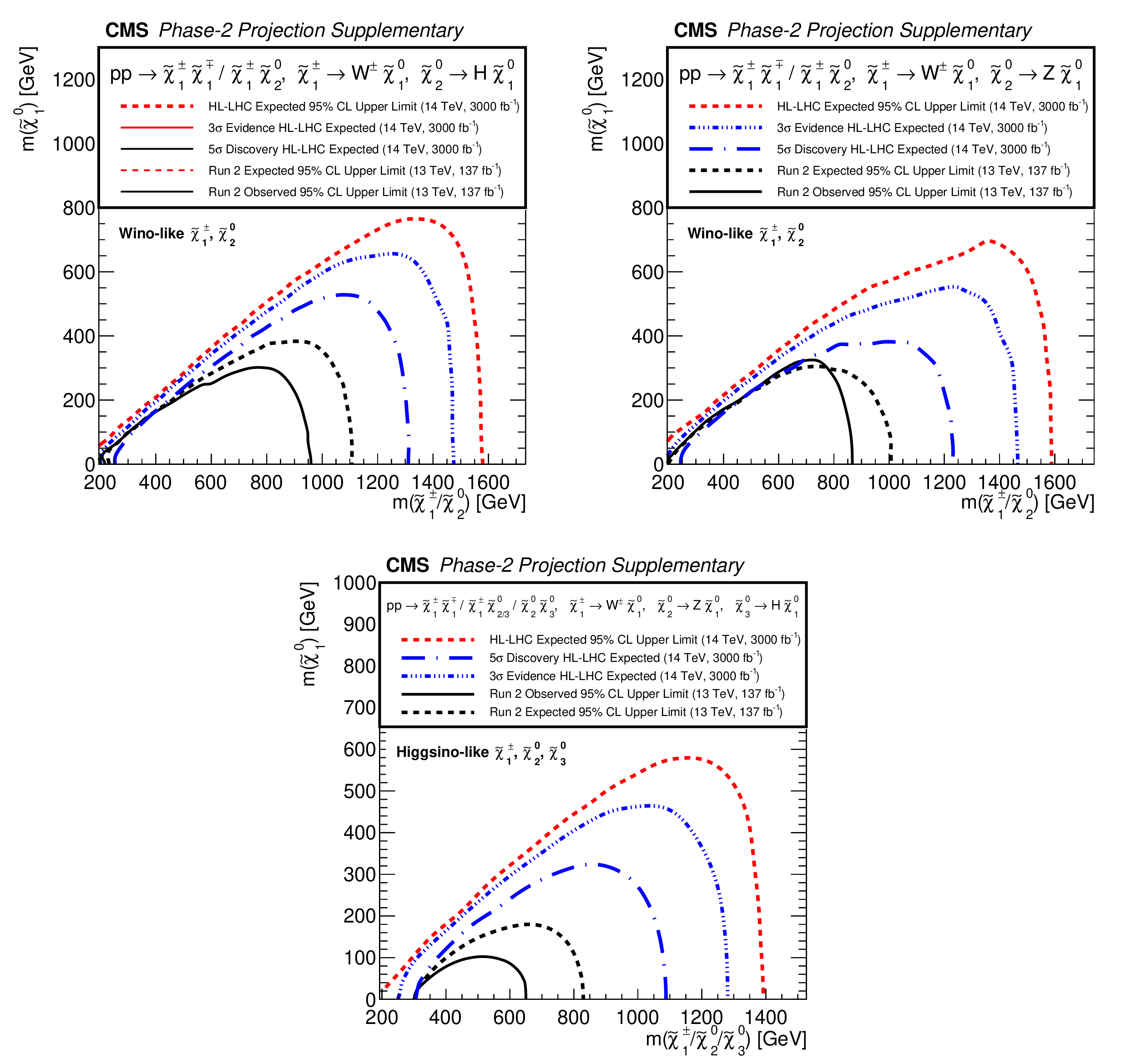
Additional Figure 20:
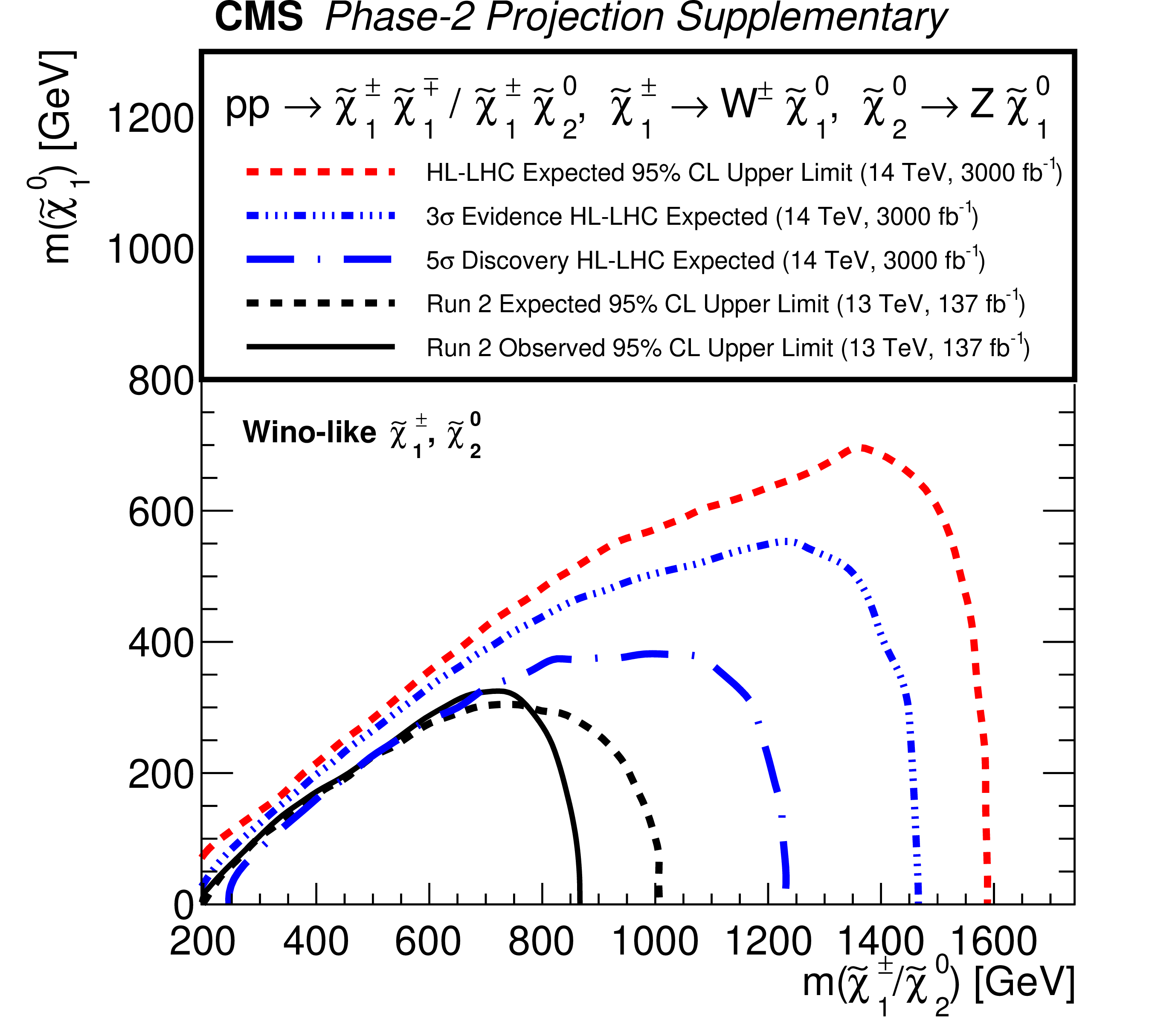
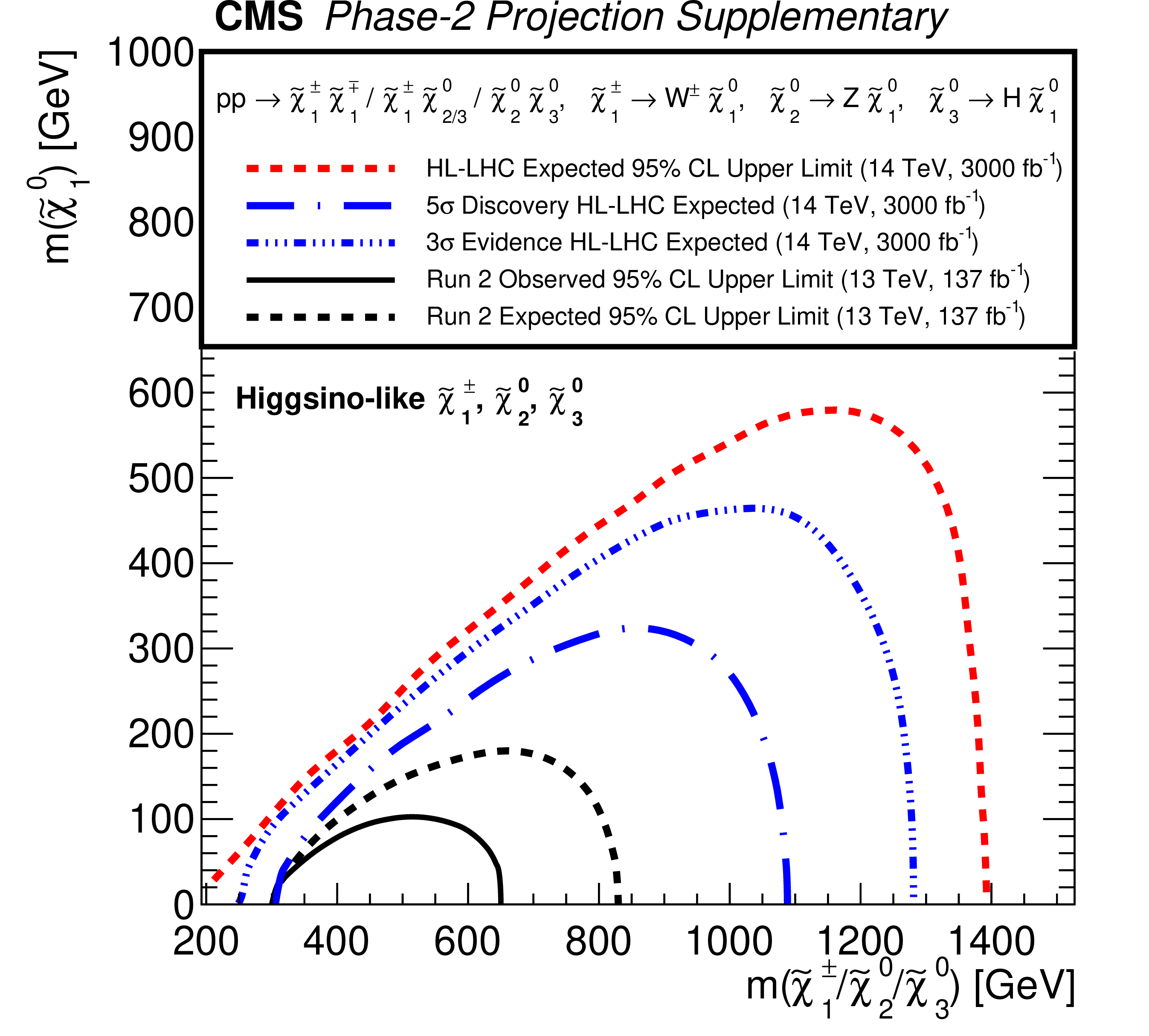
Projected 95% CL exclusion for 3$\,\text{ab}^{-1}$ (red) for mass-degenerate wino-like $ \tilde{\chi}_{1}^{\pm}{\tilde{\chi}}{1}{\mp} $ and $ \tilde{\chi}_{1}^{\pm}\tilde{\chi}_{2}^{0} $ production assuming $ \mathcal{B}(\tilde{\chi}_{2}^{0} \to \mathrm{H} \tilde{\chi}_{1}^{0}) = 100% $ (a) or $ \mathcal{B}(\tilde{\chi}_{2}^{0} \to \mathrm{Z} \tilde{\chi}_{1}^{0}) = 100% $ (b) and higgsino-like $ \tilde{\chi}_{1}^{\pm}\tilde{\chi}_{2}^{0} $, $ \tilde{\chi}_{1}^{\pm}\tilde{\chi}_{3}^{0} $, $ \tilde{\chi}_{1}^{\pm}{\tilde{\chi}}{1}{\mp} $, and $ \tilde{\chi}_{2}^{0}\tilde{\chi}_{3}^{0} $ production (c) as functions of the NLSP and LSP masses. Projections are compared to results from LHC Run 2 with 137 fb$ ^{-1} $ (black). Projected 5 $ \sigma $ and 3 $ \sigma $ expected significance curves (blue) are also included. |
png pdf |
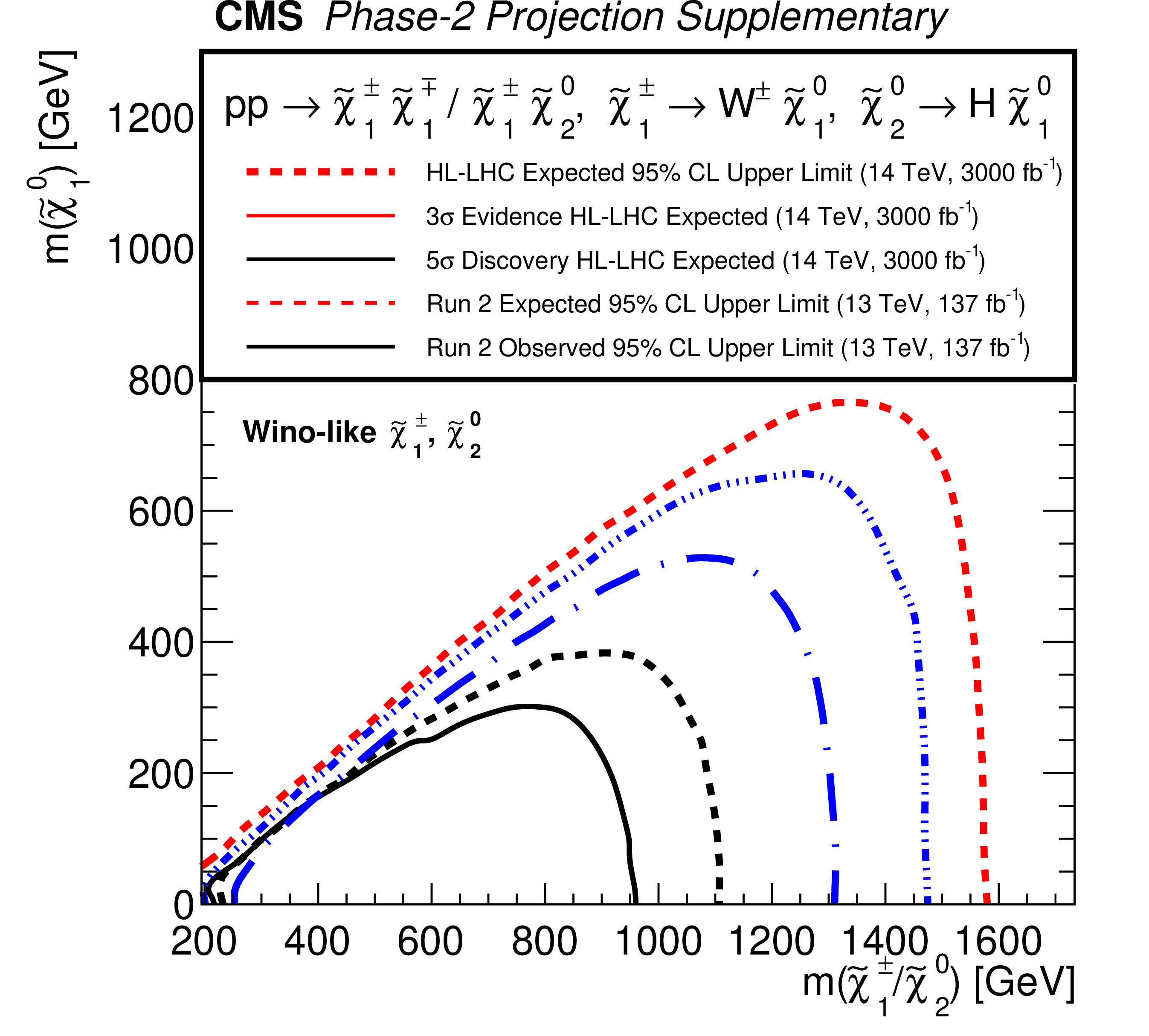
Additional Figure 20-a:
Projected 95% CL exclusion for 3$\,\text{ab}^{-1}$ (red) for mass-degenerate wino-like $ \tilde{\chi}_{1}^{\pm}{\tilde{\chi}}{1}{\mp} $ and $ \tilde{\chi}_{1}^{\pm}\tilde{\chi}_{2}^{0} $ production assuming $ \mathcal{B}(\tilde{\chi}_{2}^{0} \to \mathrm{H} \tilde{\chi}_{1}^{0}) = 100% $ (a) or $ \mathcal{B}(\tilde{\chi}_{2}^{0} \to \mathrm{Z} \tilde{\chi}_{1}^{0}) = 100% $ (b) and higgsino-like $ \tilde{\chi}_{1}^{\pm}\tilde{\chi}_{2}^{0} $, $ \tilde{\chi}_{1}^{\pm}\tilde{\chi}_{3}^{0} $, $ \tilde{\chi}_{1}^{\pm}{\tilde{\chi}}{1}{\mp} $, and $ \tilde{\chi}_{2}^{0}\tilde{\chi}_{3}^{0} $ production (c) as functions of the NLSP and LSP masses. Projections are compared to results from LHC Run 2 with 137 fb$ ^{-1} $ (black). Projected 5 $ \sigma $ and 3 $ \sigma $ expected significance curves (blue) are also included. |
png pdf |
Additional Figure 20-b:
Projected 95% CL exclusion for 3$\,\text{ab}^{-1}$ (red) for mass-degenerate wino-like $ \tilde{\chi}_{1}^{\pm}{\tilde{\chi}}{1}{\mp} $ and $ \tilde{\chi}_{1}^{\pm}\tilde{\chi}_{2}^{0} $ production assuming $ \mathcal{B}(\tilde{\chi}_{2}^{0} \to \mathrm{H} \tilde{\chi}_{1}^{0}) = 100% $ (a) or $ \mathcal{B}(\tilde{\chi}_{2}^{0} \to \mathrm{Z} \tilde{\chi}_{1}^{0}) = 100% $ (b) and higgsino-like $ \tilde{\chi}_{1}^{\pm}\tilde{\chi}_{2}^{0} $, $ \tilde{\chi}_{1}^{\pm}\tilde{\chi}_{3}^{0} $, $ \tilde{\chi}_{1}^{\pm}{\tilde{\chi}}{1}{\mp} $, and $ \tilde{\chi}_{2}^{0}\tilde{\chi}_{3}^{0} $ production (c) as functions of the NLSP and LSP masses. Projections are compared to results from LHC Run 2 with 137 fb$ ^{-1} $ (black). Projected 5 $ \sigma $ and 3 $ \sigma $ expected significance curves (blue) are also included. |
png pdf |
Additional Figure 20-c:
Projected 95% CL exclusion for 3$\,\text{ab}^{-1}$ (red) for mass-degenerate wino-like $ \tilde{\chi}_{1}^{\pm}{\tilde{\chi}}{1}{\mp} $ and $ \tilde{\chi}_{1}^{\pm}\tilde{\chi}_{2}^{0} $ production assuming $ \mathcal{B}(\tilde{\chi}_{2}^{0} \to \mathrm{H} \tilde{\chi}_{1}^{0}) = 100% $ (a) or $ \mathcal{B}(\tilde{\chi}_{2}^{0} \to \mathrm{Z} \tilde{\chi}_{1}^{0}) = 100% $ (b) and higgsino-like $ \tilde{\chi}_{1}^{\pm}\tilde{\chi}_{2}^{0} $, $ \tilde{\chi}_{1}^{\pm}\tilde{\chi}_{3}^{0} $, $ \tilde{\chi}_{1}^{\pm}{\tilde{\chi}}{1}{\mp} $, and $ \tilde{\chi}_{2}^{0}\tilde{\chi}_{3}^{0} $ production (c) as functions of the NLSP and LSP masses. Projections are compared to results from LHC Run 2 with 137 fb$ ^{-1} $ (black). Projected 5 $ \sigma $ and 3 $ \sigma $ expected significance curves (blue) are also included. |
png pdf root |
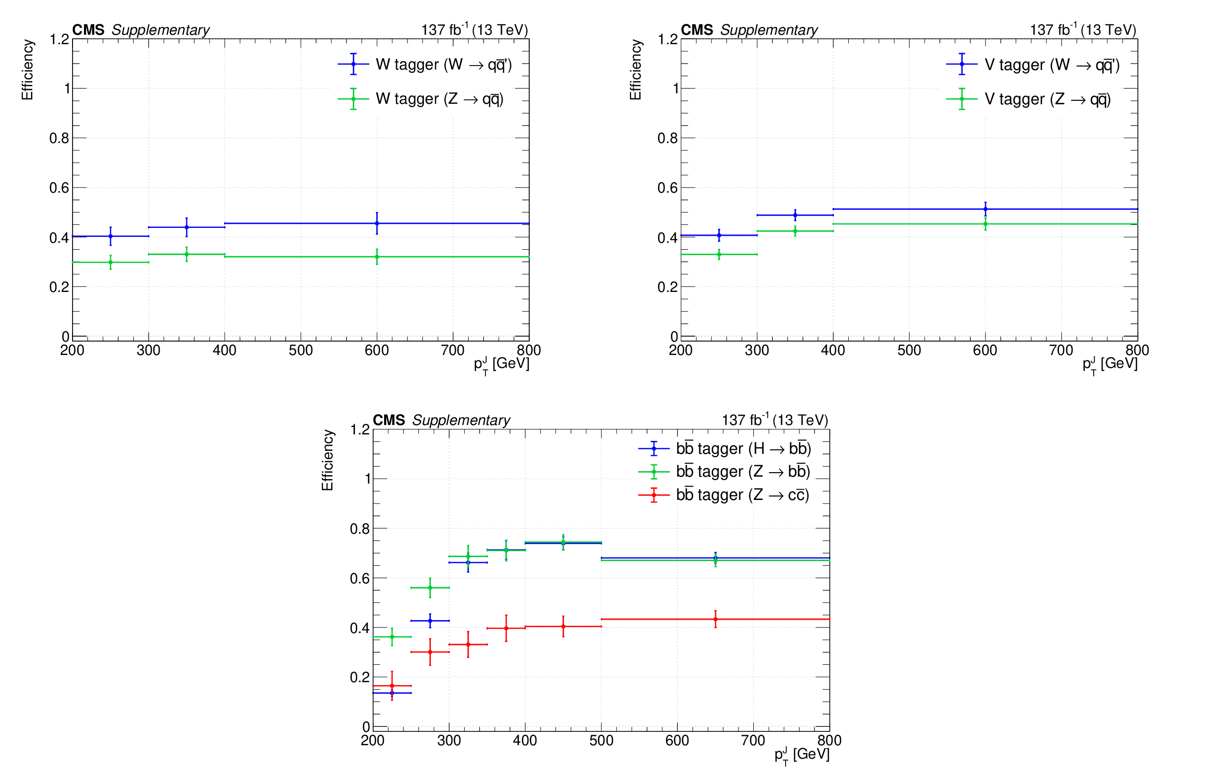
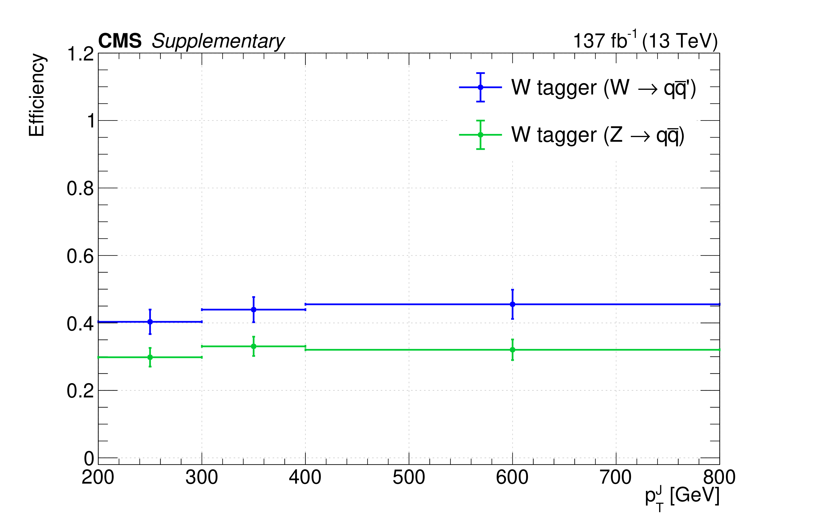
Additional Figure 21:
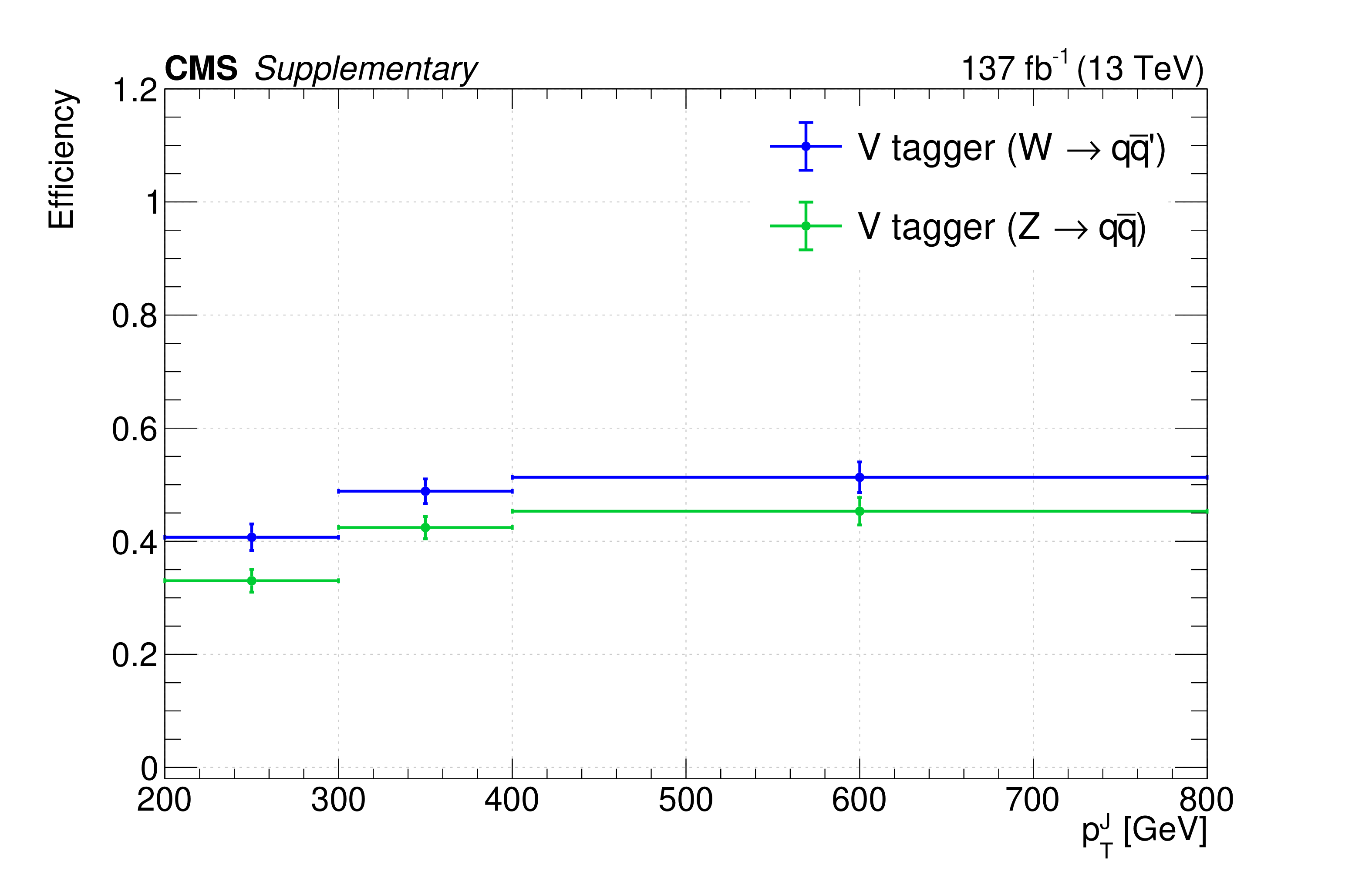
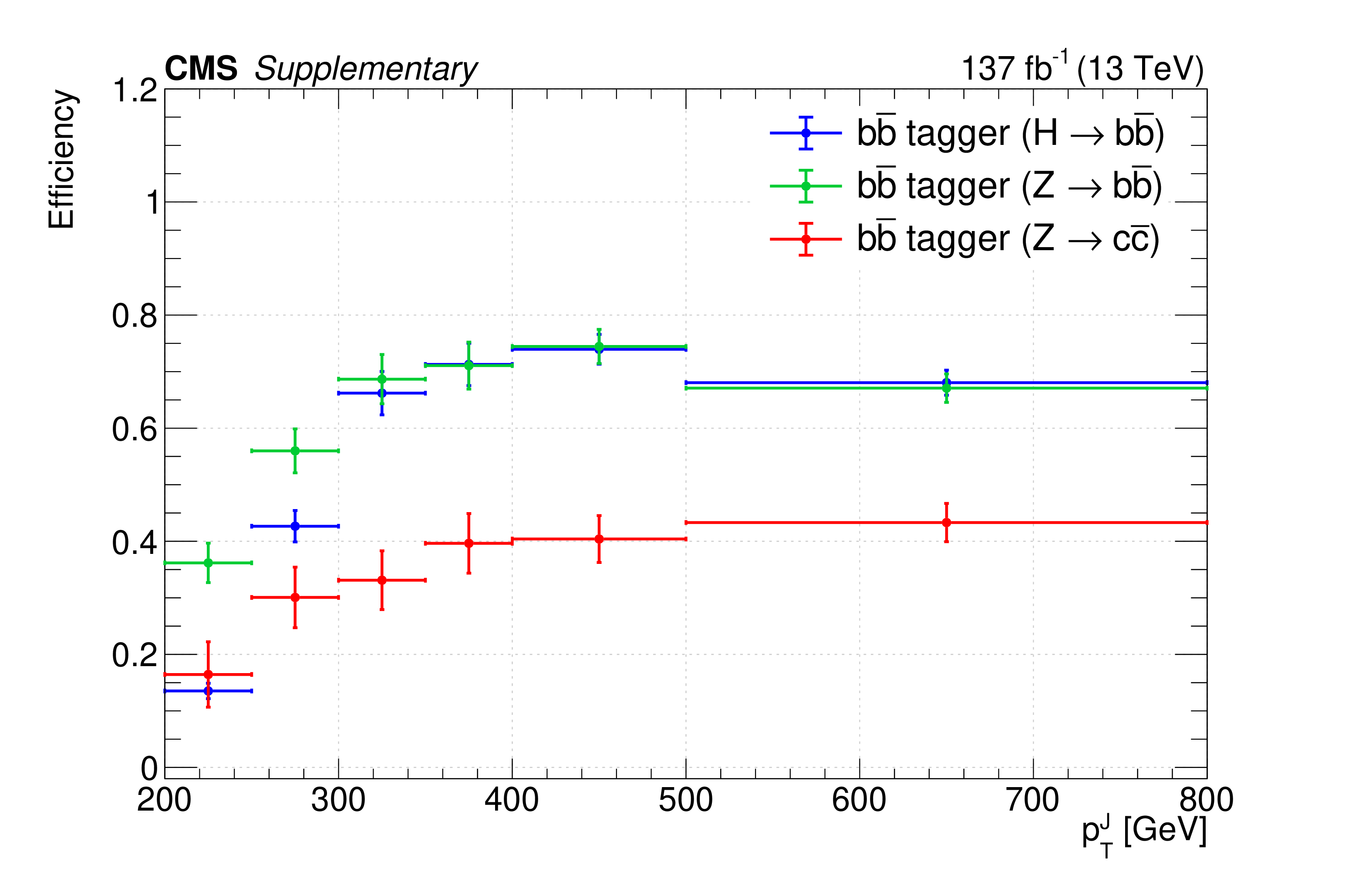
Efficiencies of the W tagger (a), V tagger (b) and $ \mathrm{b} \overline{\mathrm{b}} $ tagger (c) for tagging hadronic decays of W, Z, and H bosons. The uncertainty in each tagging efficiency is dominated by the difference between data and simulation and is considered to be correlated across $ p_{\mathrm{T}} $ bins. The efficiencies are derived with baseline selections and require the reconstructed AK8 jets to be within $ \Delta R < $ 0.6 of the generated bosons. Additionally, $ \mathrm{b} \overline{\mathrm{b}} $-tagged AK8 jets are required to be near at least one b-tagged AK4 jet that satisfies $ \Delta R(\mathrm{b}\text{ jet}, \text{AK8 jet}) < $ 0.8; W- and V-tagged AK8 jets are required to be away ($ \Delta R > $ 0.8) from all the b-tagged AK4 jets. The correlation between the W and V taggers is found to be about 80%. When the W tagger tags $ \mathrm{Z}(\mathrm{q}\overline{\mathrm{q}}) $ decays, we assign half the difference between the $ \mathrm{W}(\mathrm{q}{\overline{\mathrm{q}}}{\prime}) $ and $ \mathrm{Z}(\mathrm{q}\overline{\mathrm{q}}) $ efficiencies (blue vs.\ green in (a)) as the uncertainty, correlated across all $ p_{\mathrm{T}} $ ranges. The W- and V-tagging efficiencies are not applicable to vector bosons arising from H boson decays. |
png pdf root |
Additional Figure 21-a:
Efficiencies of the W tagger (a), V tagger (b) and $ \mathrm{b} \overline{\mathrm{b}} $ tagger (c) for tagging hadronic decays of W, Z, and H bosons. The uncertainty in each tagging efficiency is dominated by the difference between data and simulation and is considered to be correlated across $ p_{\mathrm{T}} $ bins. The efficiencies are derived with baseline selections and require the reconstructed AK8 jets to be within $ \Delta R < $ 0.6 of the generated bosons. Additionally, $ \mathrm{b} \overline{\mathrm{b}} $-tagged AK8 jets are required to be near at least one b-tagged AK4 jet that satisfies $ \Delta R(\mathrm{b}\text{ jet}, \text{AK8 jet}) < $ 0.8; W- and V-tagged AK8 jets are required to be away ($ \Delta R > $ 0.8) from all the b-tagged AK4 jets. The correlation between the W and V taggers is found to be about 80%. When the W tagger tags $ \mathrm{Z}(\mathrm{q}\overline{\mathrm{q}}) $ decays, we assign half the difference between the $ \mathrm{W}(\mathrm{q}{\overline{\mathrm{q}}}{\prime}) $ and $ \mathrm{Z}(\mathrm{q}\overline{\mathrm{q}}) $ efficiencies (blue vs.\ green in (a)) as the uncertainty, correlated across all $ p_{\mathrm{T}} $ ranges. The W- and V-tagging efficiencies are not applicable to vector bosons arising from H boson decays. |
png pdf root |
Additional Figure 21-b:
Efficiencies of the W tagger (a), V tagger (b) and $ \mathrm{b} \overline{\mathrm{b}} $ tagger (c) for tagging hadronic decays of W, Z, and H bosons. The uncertainty in each tagging efficiency is dominated by the difference between data and simulation and is considered to be correlated across $ p_{\mathrm{T}} $ bins. The efficiencies are derived with baseline selections and require the reconstructed AK8 jets to be within $ \Delta R < $ 0.6 of the generated bosons. Additionally, $ \mathrm{b} \overline{\mathrm{b}} $-tagged AK8 jets are required to be near at least one b-tagged AK4 jet that satisfies $ \Delta R(\mathrm{b}\text{ jet}, \text{AK8 jet}) < $ 0.8; W- and V-tagged AK8 jets are required to be away ($ \Delta R > $ 0.8) from all the b-tagged AK4 jets. The correlation between the W and V taggers is found to be about 80%. When the W tagger tags $ \mathrm{Z}(\mathrm{q}\overline{\mathrm{q}}) $ decays, we assign half the difference between the $ \mathrm{W}(\mathrm{q}{\overline{\mathrm{q}}}{\prime}) $ and $ \mathrm{Z}(\mathrm{q}\overline{\mathrm{q}}) $ efficiencies (blue vs.\ green in (a)) as the uncertainty, correlated across all $ p_{\mathrm{T}} $ ranges. The W- and V-tagging efficiencies are not applicable to vector bosons arising from H boson decays. |
png pdf root |
Additional Figure 21-c:
Efficiencies of the W tagger (a), V tagger (b) and $ \mathrm{b} \overline{\mathrm{b}} $ tagger (c) for tagging hadronic decays of W, Z, and H bosons. The uncertainty in each tagging efficiency is dominated by the difference between data and simulation and is considered to be correlated across $ p_{\mathrm{T}} $ bins. The efficiencies are derived with baseline selections and require the reconstructed AK8 jets to be within $ \Delta R < $ 0.6 of the generated bosons. Additionally, $ \mathrm{b} \overline{\mathrm{b}} $-tagged AK8 jets are required to be near at least one b-tagged AK4 jet that satisfies $ \Delta R(\mathrm{b}\text{ jet}, \text{AK8 jet}) < $ 0.8; W- and V-tagged AK8 jets are required to be away ($ \Delta R > $ 0.8) from all the b-tagged AK4 jets. The correlation between the W and V taggers is found to be about 80%. When the W tagger tags $ \mathrm{Z}(\mathrm{q}\overline{\mathrm{q}}) $ decays, we assign half the difference between the $ \mathrm{W}(\mathrm{q}{\overline{\mathrm{q}}}{\prime}) $ and $ \mathrm{Z}(\mathrm{q}\overline{\mathrm{q}}) $ efficiencies (blue vs.\ green in (a)) as the uncertainty, correlated across all $ p_{\mathrm{T}} $ ranges. The W- and V-tagging efficiencies are not applicable to vector bosons arising from H boson decays. |
| Additional Tables | |
png pdf |
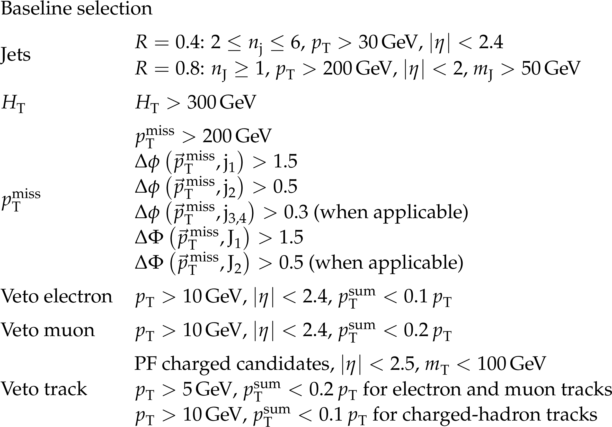
Additional Table 1:
Summary of the baseline selection requirements imposed on the reconstructed physics objects for this search. Here $ R $ is the distance parameter of the anti-$ k_{\mathrm{T}} $ algorithm. Electron and muon candidates as well as $ \tau_\mathrm{h} $ candidates and isolated tracks are as defined in the main body of the text. The $ \mathrm{i} $-th highest-$ p_{\mathrm{T}} $ jets reconstructed by the anti-$ k_{\mathrm{T}} $ algorithm with $ R = $ 0.4 and 0.8 are denoted by ${\mathrm {j}_{\mathrm {i}}}$ and ${\mathrm {J}_{\mathrm {i}}}$, respectively. Similarly, $ n_\text{j} $ and $ n_\text{J} $ indicate the number of selected jets with $ R = $ 0.4 and 0.8, respectively. |
png pdf |
Additional Table 2:
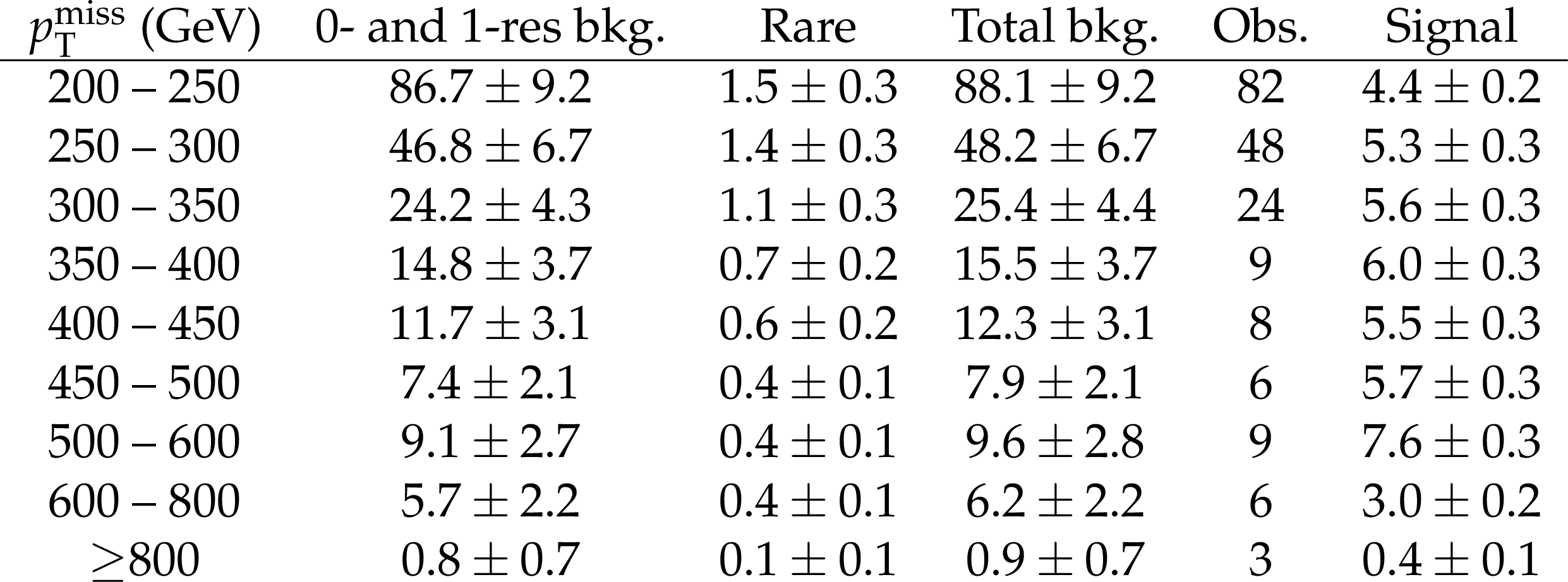
Observations and SM background predictions derived from the fit to the data in the CRs in the b-veto SR. The column labeled ``Signal'' provides the expected signal yields from the TChiWZ model with an NLSP mass of 600 GeV and an LSP mass of 100 GeV. The uncertainties in the SM background predictions include both statistical and systematic uncertainties. For the signal, only the statistical uncertainties from simulation are listed. |
png pdf |
Additional Table 3:
Observations and SM background predictions derived from the fit to the data in the CRs in each of the b-tag SRs. The column labeled ``Signal'' provides the expected signal yields from the TChiWH model with an NLSP mass of 1000 GeV and an LSP mass of 100 GeV. The uncertainties in the SM background predictions include both statistical and systematic uncertainties. For the signal, only the statistical uncertainties from simulation are listed. |
png pdf |
Additional Table 4:
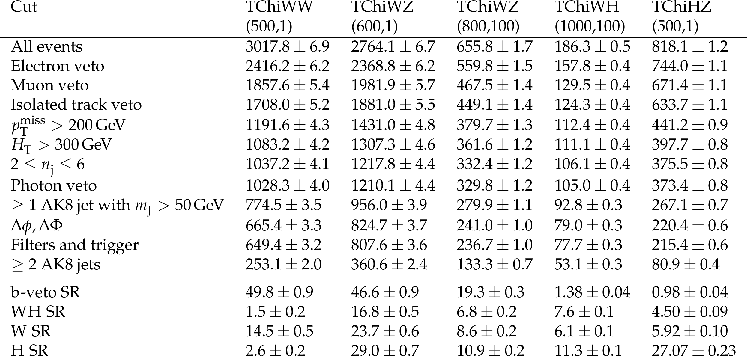
Cut flow table for selected signal samples, which are denoted in the top row by the name of the model followed by the assumed masses of the NLSP and LSP. The event yields are scaled to 137 fb$^{-1}$. The last four rows correspond to the total yield in different search region categories and they are not sequential. All the uncertainties are statistical uncertainties. The event yields are based on higgsino-like NLSPs for the TChiHZ model and wino-like NLSPs for others. |
| References | ||||
| 1 | P. Ramond | Dual theory for free fermions | PRD 3 (1971) 2415 | |
| 2 | Y. A. Golfand and E. P. Likhtman | Extension of the algebra of Poincaré group generators and violation of P invariance | JETP Lett. 13 (1971) 323 | |
| 3 | A. Neveu and J. H. Schwarz | Factorizable dual model of pions | NPB 31 (1971) 86 | |
| 4 | D. V. Volkov and V. P. Akulov | Possible universal neutrino interaction | JETP Lett. 16 (1972) 438 | |
| 5 | J. Wess and B. Zumino | A Lagrangian model invariant under supergauge transformations | PLB 49 (1974) 52 | |
| 6 | J. Wess and B. Zumino | Supergauge transformations in four dimensions | NPB 70 (1974) 39 | |
| 7 | P. Fayet | Supergauge invariant extension of the Higgs mechanism and a model for the electron and its neutrino | NPB 90 (1975) 104 | |
| 8 | P. Fayet and S. Ferrara | Supersymmetry | Phys. Rept. 32 (1977) 249 | |
| 9 | H. P. Nilles | Supersymmetry, supergravity and particle physics | Phys. Rept. 110 (1984) 1 | |
| 10 | S. P. Martin | A supersymmetry primer | Adv. Ser. Direct. High Energy Phys. 21 (2010) 1 | hep-ph/9709356 |
| 11 | M. Papucci, J. T. Ruderman, and A. Weiler | Natural SUSY endures | JHEP 09 (2012) 035 | 1110.6926 |
| 12 | H. Baer et al. | Natural SUSY with a bino- or wino-like LSP | PRD 91 (2015) 075005 | 1501.06357 |
| 13 | H. Baer, V. Barger, N. Nagata, and M. Savoy | Phenomenological profile of top squarks from natural supersymmetry at the LHC | PRD 95 (2017) 055012 | 1611.08511 |
| 14 | ATLAS Collaboration | Search for bottom-squark pair production with the ATLAS detector in final states containing Higgs bosons, $ b $-jets and missing transverse momentum | JHEP 12 (2019) 060 | 1908.03122 |
| 15 | ATLAS Collaboration | Search for a scalar partner of the top quark in the all-hadronic $ t\bar{t} $ plus missing transverse momentum final state at $ \sqrt{s}=$ 13 TeV with the ATLAS detector | EPJC 80 (2020) 737 | 2004.14060 |
| 16 | ATLAS Collaboration | Search for squarks and gluinos in final states with jets and missing transverse momentum using 139 fb $ ^-1 $ of $ \sqrt{s} =$ 13 TeV pp collision data with the ATLAS detector | JHEP 02 (2021) 143 | 2010.14293 |
| 17 | ATLAS Collaboration | Search for new phenomena with top quark pairs in final states with one lepton, jets, and missing transverse momentum in pp collisions at $ \sqrt{s}=$ 13 TeV with the ATLAS detector | JHEP 04 (2021) 174 | 2012.03799 |
| 18 | ATLAS Collaboration | Search for squarks and gluinos in final states with one isolated lepton, jets, and missing transverse momentum at $ \sqrt{s}=$ 13 TeV with the ATLAS detector | EPJC 81 (2021) 600 | 2101.01629 |
| 19 | ATLAS Collaboration | Search for new phenomena in final states with $ b $-jets and missing transverse momentum in $ \sqrt{s}=$ 13 TeV pp collisions with the ATLAS detector | JHEP 05 (2021) 093 | 2101.12527 |
| 20 | ATLAS Collaboration | Search for new phenomena in events with two opposite-charge leptons, jets and missing transverse momentum in pp collisions at $ \sqrt{s}=$ 13 TeV with the ATLAS detector | JHEP 04 (2021) 165 | 2102.01444 |
| 21 | ATLAS Collaboration | Search for bottom-squark pair production in pp collision events at $ \sqrt{s} = $ 13 TeV with hadronically decaying $ \tau $-leptons, $ b $-jets and missing transverse momentum using the ATLAS detector | PRD 104 (2021) 032014 | 2103.08189 |
| 22 | CMS Collaboration | Search for supersymmetry in proton-proton collisions at 13 TeV in final states with jets and missing transverse momentum | JHEP 10 (2019) 244 | CMS-SUS-19-006 1908.04722 |
| 23 | CMS Collaboration | Searches for physics beyond the standard model with the $ M_\mathrm{T2} $ variable in hadronic final states with and without disappearing tracks in proton-proton collisions at $ \sqrt{s}= $ 13 TeV | EPJC 80 (2020) 3 | CMS-SUS-19-005 1909.03460 |
| 24 | CMS Collaboration | Search for supersymmetry in pp collisions at $ \sqrt{s}= $ 13 TeV with 137 fb $ ^-1 $ in final states with a single lepton using the sum of masses of large-radius jets | PRD 101 (2020) 052010 | CMS-SUS-19-007 1911.07558 |
| 25 | CMS Collaboration | Search for direct top squark pair production in events with one lepton, jets, and missing transverse momentum at 13 TeV with the CMS experiment | JHEP 05 (2020) 032 | CMS-SUS-19-009 1912.08887 |
| 26 | CMS Collaboration | Search for top squark pair production using dilepton final states in $ \text p\text p $ collision data collected at $ \sqrt{s}=$ 13 TeV | EPJC 81 (2021) 3 | CMS-SUS-19-011 2008.05936 |
| 27 | CMS Collaboration | Search for top squark production in fully hadronic final states in proton-proton collisions at $ \sqrt{s} = $ 13 TeV | PRD 104 (2021) 052001 | CMS-SUS-19-010 2103.01290 |
| 28 | CMS Collaboration | Combined searches for the production of supersymmetric top quark partners in proton-proton collisions at $ \sqrt{s} = $ 13 TeV | EPJC 81 (2021) 970 | CMS-SUS-20-002 2107.10892 |
| 29 | G. R. Farrar and P. Fayet | Phenomenology of the production, decay, and detection of new hadronic states associated with supersymmetry | PLB 76 (1978) 575 | |
| 30 | ATLAS Collaboration | Search for electroweak production of supersymmetric particles in final states with two or three leptons at $ \sqrt{s}=$ 13 TeV with the ATLAS detector | EPJC 78 (2018) 995 | 1803.02762 |
| 31 | ATLAS Collaboration | Search for chargino-neutralino production using recursive jigsaw reconstruction in final states with two or three charged leptons in proton-proton collisions at $ \sqrt{s}=$ 13 TeV with the ATLAS detector | PRD 98 (2018) 092012 | 1806.02293 |
| 32 | ATLAS Collaboration | Search for chargino and neutralino production in final states with a Higgs boson and missing transverse momentum at $ \sqrt{s} = $ 13 TeV with the ATLAS detector | PRD 100 (2019) 012006 | 1812.09432 |
| 33 | ATLAS Collaboration | Search for electroweak production of charginos and sleptons decaying into final states with two leptons and missing transverse momentum in $ \sqrt{s}=$ 13 TeV pp collisions using the ATLAS detector | EPJC 80 (2020) 123 | 1908.08215 |
| 34 | ATLAS Collaboration | Search for direct production of electroweakinos in final states with one lepton, missing transverse momentum and a Higgs boson decaying into two $ b $-jets in pp collisions at $ \sqrt{s}=$ 13 TeV with the ATLAS detector | EPJC 80 (2020) 691 | 1909.09226 |
| 35 | ATLAS Collaboration | Search for chargino-neutralino production with mass splittings near the electroweak scale in three-lepton final states in $ \sqrt{s}=$ 13 TeV pp collisions with the ATLAS detector | PRD 101 (2020) 072001 | 1912.08479 |
| 36 | ATLAS Collaboration | Search for chargino--neutralino pair production in final states with three leptons and missing transverse momentum in $ \sqrt{s} = $ 13 TeV pp collisions with the ATLAS detector | EPJC 81 (2021) 1118 | 2106.01676 |
| 37 | ATLAS Collaboration | Search for charginos and neutralinos in final states with two boosted hadronically decaying bosons and missing transverse momentum in pp collisions at $ \sqrt{s}=$ 13 TeV with the ATLAS detector | PRD 104 (2021) 112010 | 2108.07586 |
| 38 | ATLAS Collaboration | Searches for new phenomena in events with two leptons, jets, and missing transverse momentum in 139 fb$^{-1}$ of $ \sqrt{s}=$ 13 TeV pp collisions with the ATLAS detector | Submitted to Eur. Phys. J. C, 2022 | 2204.13072 |
| 39 | CMS Collaboration | Search for electroweak production of charginos and neutralinos in WH events in proton-proton collisions at $ \sqrt{s}=$ 13 TeV | JHEP 11 (2017) 029 | CMS-SUS-16-043 1706.09933 |
| 40 | CMS Collaboration | Search for electroweak production of charginos and neutralinos in multilepton final states in proton-proton collisions at $ \sqrt{s}=$ 13 TeV | JHEP 03 (2018) 166 | CMS-SUS-16-039 1709.05406 |
| 41 | CMS Collaboration | Combined search for electroweak production of charginos and neutralinos in proton-proton collisions at $ \sqrt{s}=$ 13 TeV | JHEP 03 (2018) 160 | CMS-SUS-17-004 1801.03957 |
| 42 | CMS Collaboration | Searches for pair production of charginos and top squarks in final states with two oppositely charged leptons in proton-proton collisions at $ \sqrt{s}= $ 13 TeV | JHEP 11 (2018) 079 | CMS-SUS-17-010 1807.07799 |
| 43 | CMS Collaboration | Search for supersymmetry in final states with two oppositely charged same-flavor leptons and missing transverse momentum in proton-proton collisions at $ \sqrt{s} = $ 13 TeV | JHEP 04 (2021) 123 | CMS-SUS-20-001 2012.08600 |
| 44 | CMS Collaboration | Search for electroweak production of charginos and neutralinos in proton-proton collisions at $ \sqrt{s} = $ 13 TeV | JHEP 04 (2022) 147 | CMS-SUS-19-012 2106.14246 |
| 45 | CMS Collaboration | Search for chargino-neutralino production in events with Higgs and W bosons using 137 fb $ ^-1 $ of proton-proton collisions at $ \sqrt{s} = $ 13 TeV | JHEP 10 (2021) 045 | CMS-SUS-20-003 2107.12553 |
| 46 | ATLAS Collaboration | Search for pair production of higgsinos in final states with at least three $ b $-tagged jets in $ \sqrt{s} = $ 13 TeV pp collisions using the ATLAS detector | PRD 98 (2018) 092002 | 1806.04030 |
| 47 | CMS Collaboration | Searches for electroweak neutralino and chargino production in channels with Higgs, Z, and W bosons in pp collisions at 8 TeV | PRD 90 (2014) 092007 | CMS-SUS-14-002 1409.3168 |
| 48 | CMS Collaboration | Search for higgsino pair production in pp collisions at $ \sqrt{s} $ = 13 TeV in final states with large missing transverse momentum and two Higgs bosons decaying via $ H \to b \bar b $ | PRD 97 (2018) 032007 | CMS-SUS-16-044 1709.04896 |
| 49 | CMS Collaboration | Identification of heavy, energetic, hadronically decaying particles using machine-learning techniques | JINST 15 (2020) P06005 | CMS-JME-18-002 2004.08262 |
| 50 | CMS Collaboration | HEPData record for this analysis | link | |
| 51 | J. Alwall et al. | The automated computation of tree-level and next-to-leading order differential cross sections, and their matching to parton shower simulations | JHEP 07 (2014) 079 | 1405.0301 |
| 52 | P. Nason | A new method for combining NLO QCD with shower Monte Carlo algorithms | JHEP 11 (2004) 040 | hep-ph/0409146 |
| 53 | S. Frixione, P. Nason, and C. Oleari | Matching NLO QCD computations with parton shower simulations: the POWHEG method | JHEP 11 (2007) 070 | 0709.2092 |
| 54 | S. Alioli, P. Nason, C. Oleari, and E. Re | A general framework for implementing NLO calculations in shower Monte Carlo programs: the POWHEG BOX | JHEP 06 (2010) 043 | 1002.2581 |
| 55 | S. Alioli, P. Nason, C. Oleari, and E. Re | NLO single-top production matched with shower in POWHEG: $ s $- and $ t $-channel contributions | JHEP 09 (2009) 111 | 0907.4076 |
| 56 | E. Re | Single-top Wt-channel production matched with parton showers using the POWHEG method | EPJC 71 (2011) 1547 | 1009.2450 |
| 57 | T. Melia, P. Nason, R. Röntsch, and G. Zanderighi | $W^+W^- $, $WZ$ and $ZZ$ production in the POWHEG BOX | JHEP 11 (2011) 078 | 1107.5051 |
| 58 | P. Nason and G. Zanderighi | $W^+W^- $, $ WZ $ and $ ZZ $ production in the POWHEG-BOX-V2 | EPJC 74 (2014) 2702 | 1311.1365 |
| 59 | H. B. Hartanto, B. Jäger, L. Reina, and D. Wackeroth | Higgs boson production in association with top quarks in the POWHEG BOX | PRD 91 (2015) 094003 | 1501.04498 |
| 60 | NNPDF Collaboration | Parton distributions for the LHC run II | JHEP 04 (2015) 040 | 1410.8849 |
| 61 | NNPDF Collaboration | Parton distributions from high-precision collider data | EPJC 77 (2017) 663 | 1706.00428 |
| 62 | T. Sjöstrand et al. | An introduction to PYTHIA 8.2 | Comput. Phys. Commun. 191 (2015) 159 | 1410.3012 |
| 63 | CMS Collaboration | Event generator tunes obtained from underlying event and multiparton scattering measurements | EPJC 76 (2016) 155 | CMS-GEN-14-001 1512.00815 |
| 64 | CMS Collaboration | Extraction and validation of a new set of CMS PYTHIA 8 tunes from underlying-event measurements | EPJC 80 (2020) 4 | CMS-GEN-17-001 1903.12179 |
| 65 | GEANT4 Collaboration | GEANT4 --- a simulation toolkit | NIM A 506 (2003) 250 | |
| 66 | S. Quackenbush, R. Gavin, Y. Li, and F. Petriello | W physics at the LHC with FEWZ 2.1 | Comput. Phys. Commun. 184 (2013) 209 | 1201.5896 |
| 67 | R. Gavin, Y. Li, F. Petriello, and S. Quackenbush | FEWZ 2.0: a code for hadronic Z production at next-to-next-to-leading order | Comput. Phys. Commun. 182 (2011) 2388 | 1011.3540 |
| 68 | Y. Li and F. Petriello | Combining QCD and electroweak corrections to dilepton production in FEWZ | PRD 86 (2012) 094034 | 1208.5967 |
| 69 | T. Gehrmann et al. | $W^+W^- $ production at hadron colliders in next to next to leading order QCD | PRL 113 (2014) 212001 | 1408.5243 |
| 70 | J. M. Campbell, R. K. Ellis, and C. Williams | Vector boson pair production at the LHC | JHEP 07 (2011) 018 | 1105.0020 |
| 71 | M. Beneke, P. Falgari, S. Klein, and C. Schwinn | Hadronic top-quark pair production with NNLL threshold resummation | NPB 855 (2012) 695 | 1109.1536 |
| 72 | M. Cacciari et al. | Top-pair production at hadron colliders with next-to-next-to-leading logarithmic soft-gluon resummation | PLB 710 (2012) 612 | 1111.5869 |
| 73 | P. Bärnreuther, M. Czakon, and A. Mitov | Percent-level-precision physics at the Tevatron: next-to-next-to-leading order QCD corrections to $ \mathrm{q}\overline{\mathrm{q}} \to {\mathrm{t}\overline{\mathrm{t}}}$+X | PRL 109 (2012) 132001 | 1204.5201 |
| 74 | M. Czakon and A. Mitov | NNLO corrections to top-pair production at hadron colliders: the all-fermionic scattering channels | JHEP 12 (2012) 054 | 1207.0236 |
| 75 | M. Czakon and A. Mitov | NNLO corrections to top pair production at hadron colliders: the quark-gluon reaction | JHEP 01 (2013) 080 | 1210.6832 |
| 76 | M. Czakon, P. Fiedler, and A. Mitov | Total top-quark pair-production cross section at hadron colliders through $ O(\alpha_\mathrm{S}^4) $ | PRL 110 (2013) 252004 | 1303.6254 |
| 77 | M. Czakon and A. Mitov | Top++: a program for the calculation of the top-pair cross-section at hadron colliders | Comput. Phys. Commun. 185 (2014) 2930 | 1112.5675 |
| 78 | A. Kulesza et al. | Associated production of a top quark pair with a heavy electroweak gauge boson at NLO+NNLL accuracy | EPJC 79 (2019) 249 | 1812.08622 |
| 79 | LHC Higgs Cross Section Working Group | Handbook of LHC Higgs cross sections: 4. Deciphering the nature of the Higgs sector | CERN Report CERN-2017-002-M, 2016 link |
1610.07922 |
| 80 | R. Frederix and S. Frixione | Merging meets matching in MC@NLO | JHEP 12 (2012) 061 | 1209.6215 |
| 81 | J. Alwall et al. | Comparative study of various algorithms for the merging of parton showers and matrix elements in hadronic collisions | EPJC 53 (2008) 473 | 0706.2569 |
| 82 | S. Abdullin et al. | The fast simulation of the CMS detector at LHC | J. Phys. Conf. Ser. 331 (2011) 032049 | |
| 83 | A. Giammanco | The fast simulation of the CMS experiment | J. Phys. Conf. Ser. 513 (2014) 022012 | |
| 84 | W. Beenakker et al. | Production of charginos, neutralinos, and sleptons at hadron colliders | PRL 83 (1999) 3780 | hep-ph/9906298 |
| 85 | J. Debove, B. Fuks, and M. Klasen | Threshold resummation for gaugino pair production at hadron colliders | NPB 842 (2011) 51 | 1005.2909 |
| 86 | B. Fuks, M. Klasen, D. R. Lamprea, and M. Rothering | Gaugino production in proton-proton collisions at a center-of-mass energy of 8 TeV | JHEP 10 (2012) 081 | 1207.2159 |
| 87 | B. Fuks, M. Klasen, D. R. Lamprea, and M. Rothering | Precision predictions for electroweak superpartner production at hadron colliders with Resummino | EPJC 73 (2013) 2480 | 1304.0790 |
| 88 | J. Fiaschi and M. Klasen | Neutralino-chargino pair production at NLO+NLL with resummation-improved parton density functions for LHC Run II | PRD 98 (2018) 055014 | 1805.11322 |
| 89 | N. Arkani-Hamed et al. | MARMOSET: the path from LHC data to the new standard model via on-shell effective theories | , 2007 | hep-ph/0703088 |
| 90 | J. Alwall, P. C. Schuster, and N. Toro | Simplified models for a first characterization of new physics at the LHC | PRD 79 (2009) 075020 | 0810.3921 |
| 91 | J. Alwall, M.-P. Le, M. Lisanti, and J. G. Wacker | Model-independent jets plus missing energy searches | PRD 79 (2009) 015005 | 0809.3264 |
| 92 | D. Alves et al. | Simplified models for LHC new physics searches | JPG 39 (2012) 105005 | 1105.2838 |
| 93 | CMS Collaboration | Interpretation of searches for supersymmetry with simplified models | PRD 88 (2013) 052017 | CMS-SUS-11-016 1301.2175 |
| 94 | T. Han, S. Padhi, and S. Su | Electroweakinos in the light of the Higgs boson | PRD 88 (2013) 115010 | 1309.5966 |
| 95 | P. Agrawal, J. Fan, M. Reece, and W. Xue | Deciphering the MSSM Higgs mass at future hadron colliders | JHEP 06 (2017) 027 | 1702.05484 |
| 96 | CMS Collaboration | The CMS experiment at the CERN LHC | JINST 3 (2008) S08004 | |
| 97 | CMS Collaboration | Particle-flow reconstruction and global event description with the CMS detector | JINST 12 (2017) P10003 | CMS-PRF-14-001 1706.04965 |
| 98 | M. Cacciari, G. P. Salam, and G. Soyez | The anti-$ k_\mathrm{T}$ jet clustering algorithm | JHEP 04 (2008) 063 | 0802.1189 |
| 99 | M. Cacciari, G. P. Salam, and G. Soyez | FastJet user manual | EPJC 72 (2012) 1896 | 1111.6097 |
| 100 | CMS Collaboration | Pileup mitigation at CMS in 13 TeV data | JINST 15 (2020) P09018 | CMS-JME-18-001 2003.00503 |
| 101 | D. Bertolini, P. Harris, M. Low, and N. Tran | Pileup per particle identification | JHEP 10 (2014) 059 | 1407.6013 |
| 102 | CMS Collaboration | Jet energy scale and resolution in the CMS experiment in pp collisions at 8 TeV | JINST 12 (2017) P02014 | CMS-JME-13-004 1607.03663 |
| 103 | A. J. Larkoski, S. Marzani, G. Soyez, and J. Thaler | Soft drop | JHEP 05 (2014) 146 | 1402.2657 |
| 104 | CMS Collaboration | Performance of missing transverse momentum reconstruction in proton-proton collisions at $ \sqrt{s} = $ 13 TeV using the CMS detector | JINST 14 (2019) P07004 | CMS-JME-17-001 1903.06078 |
| 105 | CMS Collaboration | Identification of heavy-flavour jets with the CMS detector in pp collisions at 13 TeV | JINST 13 (2018) P05011 | CMS-BTV-16-002 1712.07158 |
| 106 | CMS Collaboration | Performance of electron reconstruction and selection with the CMS detector in proton-proton collisions at $ \sqrt{s} = $ 8 TeV | JINST 10 (2015) P06005 | CMS-EGM-13-001 1502.02701 |
| 107 | CMS Collaboration | Performance of the CMS muon detector and muon reconstruction with proton-proton collisions at $ \sqrt{s}= $ 13 TeV | JINST 13 (2018) P06015 | CMS-MUO-16-001 1804.04528 |
| 108 | CMS Collaboration | Search for supersymmetry in pp collisions at $ \sqrt{s}=$ 13 TeV in the single-lepton final state using the sum of masses of large-radius jets | JHEP 08 (2016) 122 | CMS-SUS-15-007 1605.04608 |
| 109 | CMS Collaboration | Performance of photon reconstruction and identification with the CMS detector in proton-proton collisions at $ \sqrt{s} = $ 8 TeV | JINST 10 (2015) P08010 | CMS-EGM-14-001 1502.02702 |
| 110 | G. Louppe, M. Kagan, and K. Cranmer | Learning to pivot with adversarial networks | in Advances in Neural Information Processing Systems, volume~30, 2017 link |
1611.01046 |
| 111 | CMS Collaboration | The CMS trigger system | JINST 12 (2017) P01020 | CMS-TRG-12-001 1609.02366 |
| 112 | CMS Collaboration | Description and performance of track and primary-vertex reconstruction with the CMS tracker | JINST 9 (2014) P10009 | CMS-TRK-11-001 1405.6569 |
| 113 | CMS Collaboration | Precision luminosity measurement in proton-proton collisions at $ \sqrt{s} = $ 13 TeV in 2015 and 2016 at CMS | EPJC 81 (2021) 800 | CMS-LUM-17-003 2104.01927 |
| 114 | CMS Collaboration | CMS luminosity measurement for the 2017 data-taking period at $ \sqrt{s} = $ 13 TeV | CMS Physics Analysis Summary, 2018 CMS-PAS-LUM-17-004 |
CMS-PAS-LUM-17-004 |
| 115 | CMS Collaboration | CMS luminosity measurement for the 2018 data-taking period at $ \sqrt{s} = $ 13 TeV | CMS Physics Analysis Summary, 2019 CMS-PAS-LUM-18-002 |
CMS-PAS-LUM-18-002 |
| 116 | CMS Collaboration | Measurement of differential $ t \bar t $ production cross sections in the full kinematic range using lepton+jets events from proton-proton collisions at $ \sqrt s $ = 13 TeV | PRD 104 (2021) 092013 | CMS-TOP-20-001 2108.02803 |
| 117 | ATLAS Collaboration | Measurements of $ t\bar{t} $ differential cross-sections of highly boosted top quarks decaying to all-hadronic final states in pp collisions at $ \sqrt{s}=$ 13 TeV using the ATLAS detector | PRD 98 (2018) 012003 | 1801.02052 |
| 118 | CMS Collaboration | Measurement of the production cross section for single top quarks in association with W bosons in proton-proton collisions at $ \sqrt{s}=$ 13 TeV | JHEP 10 (2018) 117 | CMS-TOP-17-018 1805.07399 |
| 119 | CMS Collaboration | Measurements of the pp $ \to $ WZ inclusive and differential production cross section and constraints on charged anomalous triple gauge couplings at $ \sqrt{s} = $ 13 TeV | JHEP 04 (2019) 122 | CMS-SMP-18-002 1901.03428 |
| 120 | CMS Collaboration | Measurements of $ \mathrm{p} \mathrm{p} \rightarrow \mathrm{Z} \mathrm{Z} $ production cross sections and constraints on anomalous triple gauge couplings at $ \sqrt{s} = $ 13 TeV | EPJC 81 (2021) 200 | CMS-SMP-19-001 2009.01186 |
| 121 | CMS Collaboration | W $ ^+ $W $ ^- $ boson pair production in proton-proton collisions at $ \sqrt{s} = $ 13 TeV | PRD 102 (2020) 092001 | CMS-SMP-18-004 2009.00119 |
| 122 | J. S. Conway | Incorporating nuisance parameters in likelihoods for multisource spectra | in PHYSTAT, 2011 link |
1103.0354 |
| 123 | R. Barlow and C. Beeston | Fitting using finite Monte Carlo samples | Comput. Phys. Commun. 77 (1993) 219 | |
| 124 | A. L. Read | Presentation of search results: the CL $ _\text{S} $ technique | JPG 28 (2002) 2693 | |
| 125 | T. Junk | Confidence level computation for combining searches with small statistics | NIM A 434 (1999) 435 | hep-ex/9902006 |
| 126 | ATLAS Collaboration , CMS Collaboration , and LHC Higgs Combination Group | Procedure for the LHC Higgs boson search combination in Summer 2011 | Technical Report CMS-NOTE-2011-005, ATL-PHYS-PUB-2011-11, 2011 | |
| 127 | G. Cowan, K. Cranmer, E. Gross, and O. Vitells | Asymptotic formulae for likelihood-based tests of new physics | EPJC 71 (2011) 1554 | 1007.1727 |
|
|
Compact Muon Solenoid LHC, CERN |
|

|

|

|

|

|