

Compact Muon Solenoid
LHC, CERN
| CMS-HIG-22-008 ; CERN-EP-2024-035 | ||
| Constraints on anomalous Higgs boson couplings from its production and decay using the WW channel in proton-proton collisions at $ \sqrt{s} = $ 13 TeV | ||
| CMS Collaboration | ||
| 1 March 2024 | ||
| Submitted to Eur. Phys. J. C | ||
| Abstract: A study of the anomalous couplings of the Higgs boson to vector bosons, including CP-violation effects, has been conducted using its production and decay in the WW channel. This analysis is performed on proton-proton collision data collected with the CMS detector at the CERN LHC during 2016-2018 at a center-of-mass energy of 13 TeV, and corresponds to an integrated luminosity of 138 fb$ ^{-1} $. The different-flavor dilepton ($ \mathrm{e}\mu $) final state is analyzed, with dedicated categories targeting gluon fusion, electroweak vector boson fusion, and associated production with a W or Z boson. Kinematic information from associated jets is combined using matrix element techniques to increase the sensitivity to anomalous effects at the production vertex. A simultaneous measurement of four Higgs boson couplings to electroweak vector bosons is performed in the framework of a standard model effective field theory. All measurements are consistent with the expectations for the standard model Higgs boson and constraints are set on the fractional contribution of the anomalous couplings to the Higgs boson production cross section. | ||
| Links: e-print arXiv:2403.00657 [hep-ex] (PDF) ; CDS record ; inSPIRE record ; HepData record ; CADI line (restricted) ; | ||
| Figures | |
png pdf |
Figure 1:
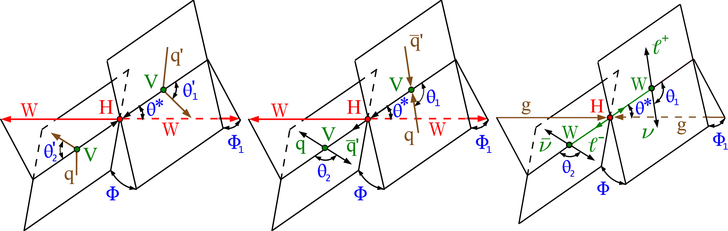
Topologies of the Higgs boson production and decay for vector boson fusion $ \mathrm{q}{\mathrm{q}^\prime}\to \mathrm{q}{\mathrm{q}^\prime} \mathrm{H} $ (left), $ \mathrm{q}\bar{\mathrm{q}}^\prime\to \mathrm{V}\mathrm{H} $ (center), and gluon fusion with decay $ \mathrm{g}\mathrm{g} \to \mathrm{H} \to 2 \ell 2\nu $ (right). For the electroweak production topologies, the intermediate vector bosons and their decays are shown in green and the $ \mathrm{H} \to \mathrm{W}\mathrm{W} $ decay is marked in red. For the $ \mathrm{g}\mathrm{g} \to \mathrm{H} \to 2 \ell 2\nu $ topology, the W boson leptonic decays are shown in green. In all cases, the incoming particles are depicted in brown and the angles characterizing kinematic distributions are marked in blue. Five angles fully characterize the orientation of the production and decay chain and are defined in the suitable rest frames. |

png pdf |
Figure 1-a:
Topologies of the Higgs boson production and decay for vector boson fusion $ \mathrm{q}{\mathrm{q}^\prime}\to \mathrm{q}{\mathrm{q}^\prime} \mathrm{H} $ (left), $ \mathrm{q}\bar{\mathrm{q}}^\prime\to \mathrm{V}\mathrm{H} $ (center), and gluon fusion with decay $ \mathrm{g}\mathrm{g} \to \mathrm{H} \to 2 \ell 2\nu $ (right). For the electroweak production topologies, the intermediate vector bosons and their decays are shown in green and the $ \mathrm{H} \to \mathrm{W}\mathrm{W} $ decay is marked in red. For the $ \mathrm{g}\mathrm{g} \to \mathrm{H} \to 2 \ell 2\nu $ topology, the W boson leptonic decays are shown in green. In all cases, the incoming particles are depicted in brown and the angles characterizing kinematic distributions are marked in blue. Five angles fully characterize the orientation of the production and decay chain and are defined in the suitable rest frames. |
png pdf |
Figure 1-b:
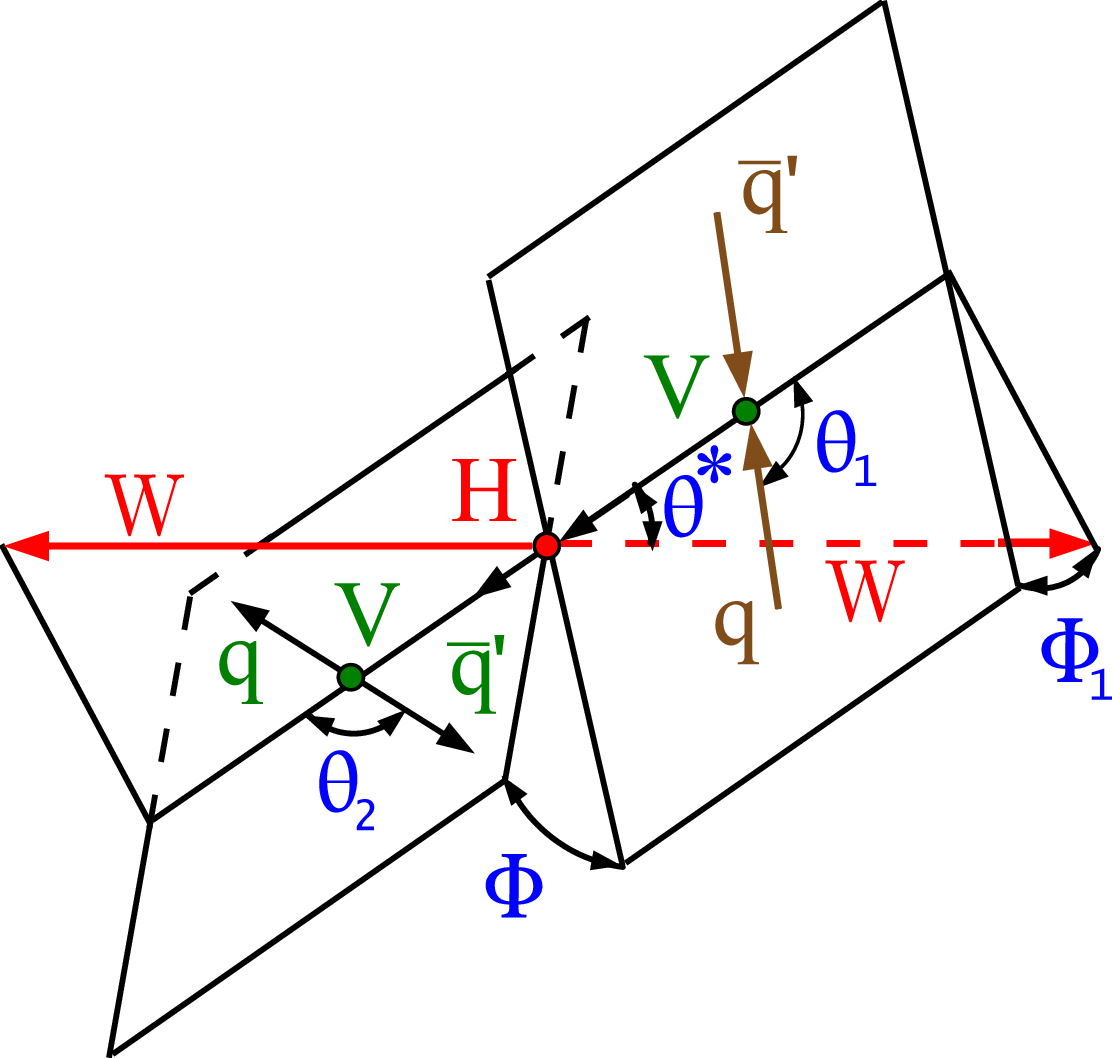
Topologies of the Higgs boson production and decay for vector boson fusion $ \mathrm{q}{\mathrm{q}^\prime}\to \mathrm{q}{\mathrm{q}^\prime} \mathrm{H} $ (left), $ \mathrm{q}\bar{\mathrm{q}}^\prime\to \mathrm{V}\mathrm{H} $ (center), and gluon fusion with decay $ \mathrm{g}\mathrm{g} \to \mathrm{H} \to 2 \ell 2\nu $ (right). For the electroweak production topologies, the intermediate vector bosons and their decays are shown in green and the $ \mathrm{H} \to \mathrm{W}\mathrm{W} $ decay is marked in red. For the $ \mathrm{g}\mathrm{g} \to \mathrm{H} \to 2 \ell 2\nu $ topology, the W boson leptonic decays are shown in green. In all cases, the incoming particles are depicted in brown and the angles characterizing kinematic distributions are marked in blue. Five angles fully characterize the orientation of the production and decay chain and are defined in the suitable rest frames. |
png pdf |
Figure 1-c:
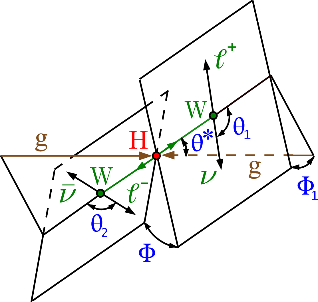
Topologies of the Higgs boson production and decay for vector boson fusion $ \mathrm{q}{\mathrm{q}^\prime}\to \mathrm{q}{\mathrm{q}^\prime} \mathrm{H} $ (left), $ \mathrm{q}\bar{\mathrm{q}}^\prime\to \mathrm{V}\mathrm{H} $ (center), and gluon fusion with decay $ \mathrm{g}\mathrm{g} \to \mathrm{H} \to 2 \ell 2\nu $ (right). For the electroweak production topologies, the intermediate vector bosons and their decays are shown in green and the $ \mathrm{H} \to \mathrm{W}\mathrm{W} $ decay is marked in red. For the $ \mathrm{g}\mathrm{g} \to \mathrm{H} \to 2 \ell 2\nu $ topology, the W boson leptonic decays are shown in green. In all cases, the incoming particles are depicted in brown and the angles characterizing kinematic distributions are marked in blue. Five angles fully characterize the orientation of the production and decay chain and are defined in the suitable rest frames. |
png pdf |
Figure 2:
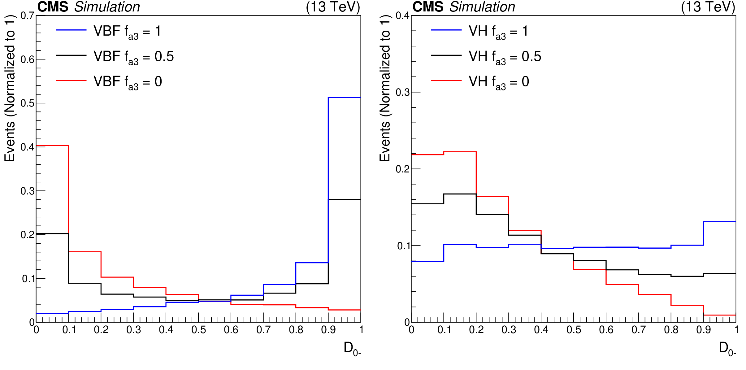
The $ \mathcal{D}_{0-} $ discriminant in the VBF (left) and Resolved VH (right) production channels for a number of VBF (left) and VH (right) signal hypotheses. Pure $ a_1 $ ($ f_{a3} = $ 0) and $ a_3 $ ($ f_{a3} = $ 1) HVV signal hypotheses are shown along with a mixed coupling hypothesis ($ f_{a3} = $ 0.5). All distributions are normalized to unity. |

png pdf |
Figure 2-a:
The $ \mathcal{D}_{0-} $ discriminant in the VBF (left) and Resolved VH (right) production channels for a number of VBF (left) and VH (right) signal hypotheses. Pure $ a_1 $ ($ f_{a3} = $ 0) and $ a_3 $ ($ f_{a3} = $ 1) HVV signal hypotheses are shown along with a mixed coupling hypothesis ($ f_{a3} = $ 0.5). All distributions are normalized to unity. |

png pdf |
Figure 2-b:
The $ \mathcal{D}_{0-} $ discriminant in the VBF (left) and Resolved VH (right) production channels for a number of VBF (left) and VH (right) signal hypotheses. Pure $ a_1 $ ($ f_{a3} = $ 0) and $ a_3 $ ($ f_{a3} = $ 1) HVV signal hypotheses are shown along with a mixed coupling hypothesis ($ f_{a3} = $ 0.5). All distributions are normalized to unity. |
png pdf |
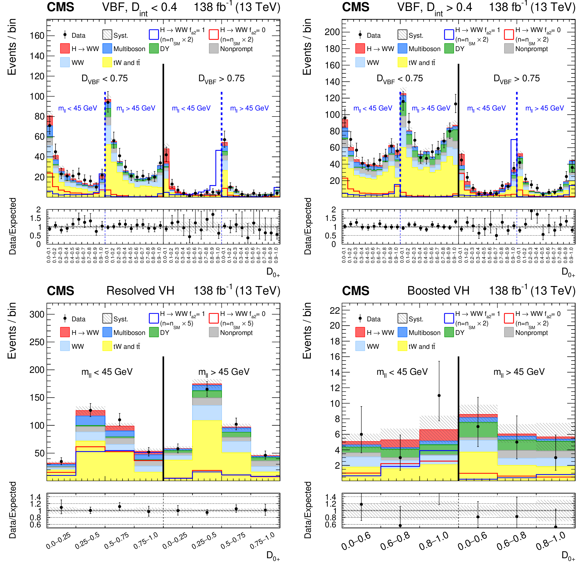
Figure 3:
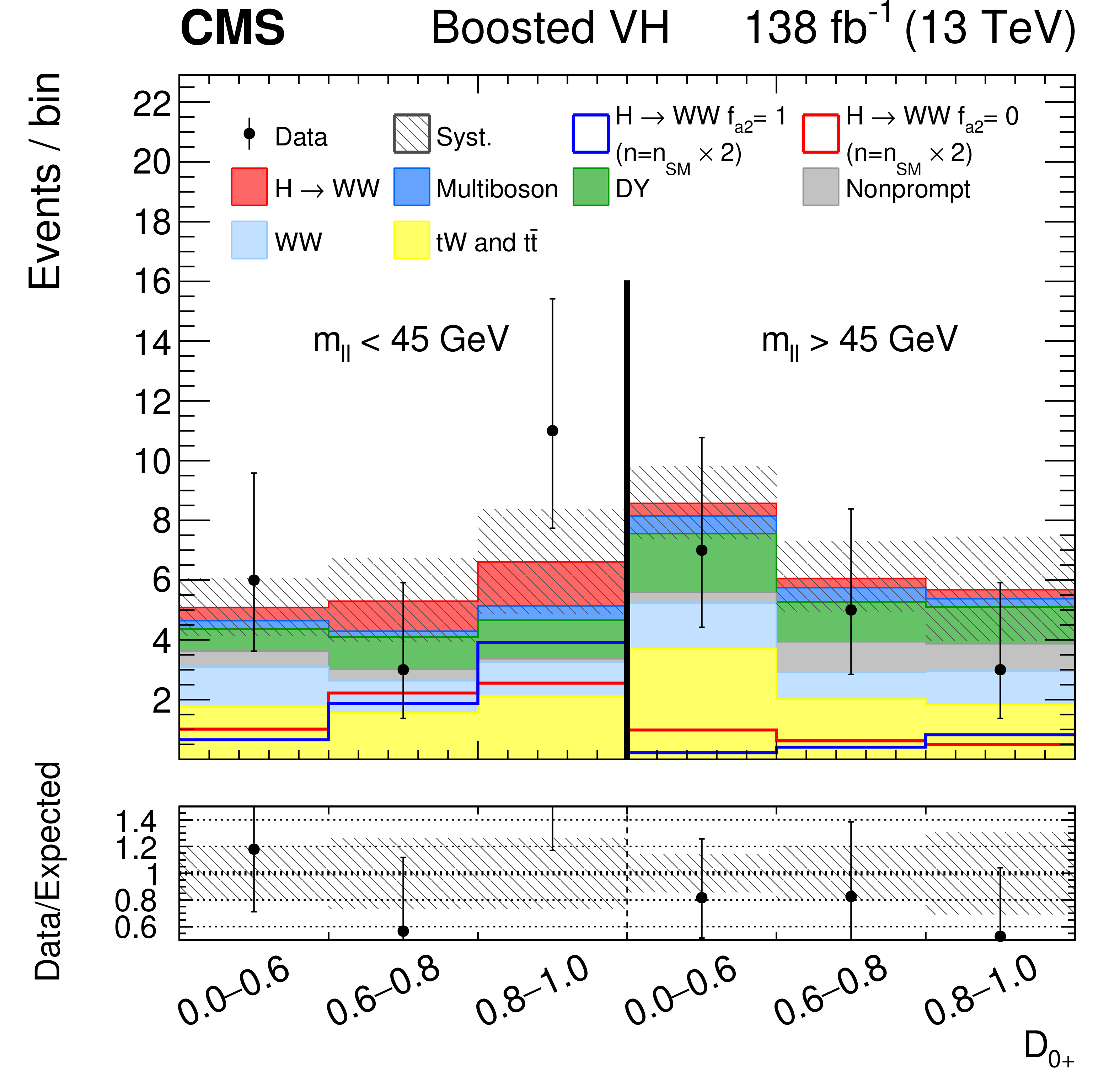
Observed and predicted distributions after fitting the data for $ [\mathcal{D}_\text{VBF}, m_{\ell\ell}, \mathcal{D}_{0+}] $ in the VBF channel (upper), and for $ [m_{\ell\ell}, \mathcal{D}_{0+}] $ in the Resolved VH (lower left) and Boosted VH (lower right) channels. For the VBF channel, the $ \mathcal{D}_{\text{int}} < $ 0.4 (left) and $ \mathcal{D}_{\text{int}} > $ 0.4 (right) categories are shown. The predicted Higgs boson signal is shown stacked on top of the background distributions. For the fit, the $ a_{1} $ and $ a_2 $ HVV coupling contributions are included. The corresponding pure $ a_{1} $ ($ f_{a2} = $ 0) and $ a_2 $ ($ f_{a2} = $ 1) signal hypotheses are also shown superimposed, their yields correspond to the predicted number of SM signal events scaled by an arbitrary factor to improve visibility. The uncertainty band corresponds to the total systematic uncertainty. The lower panel in each figure shows the ratio of the number of events observed to the total prediction. |
png pdf |
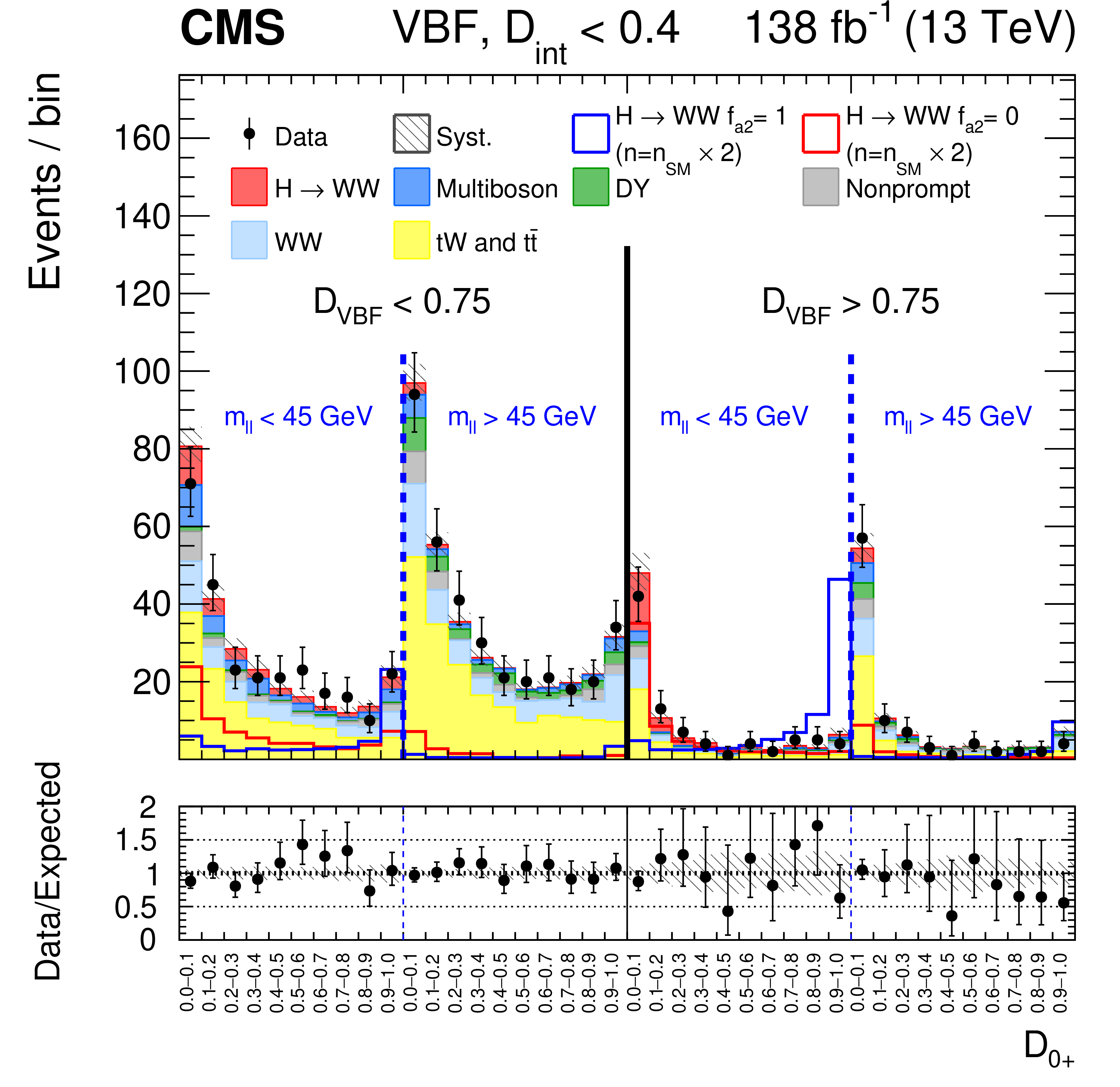
Figure 3-a:
Observed and predicted distributions after fitting the data for $ [\mathcal{D}_\text{VBF}, m_{\ell\ell}, \mathcal{D}_{0+}] $ in the VBF channel (upper), and for $ [m_{\ell\ell}, \mathcal{D}_{0+}] $ in the Resolved VH (lower left) and Boosted VH (lower right) channels. For the VBF channel, the $ \mathcal{D}_{\text{int}} < $ 0.4 (left) and $ \mathcal{D}_{\text{int}} > $ 0.4 (right) categories are shown. The predicted Higgs boson signal is shown stacked on top of the background distributions. For the fit, the $ a_{1} $ and $ a_2 $ HVV coupling contributions are included. The corresponding pure $ a_{1} $ ($ f_{a2} = $ 0) and $ a_2 $ ($ f_{a2} = $ 1) signal hypotheses are also shown superimposed, their yields correspond to the predicted number of SM signal events scaled by an arbitrary factor to improve visibility. The uncertainty band corresponds to the total systematic uncertainty. The lower panel in each figure shows the ratio of the number of events observed to the total prediction. |
png pdf |
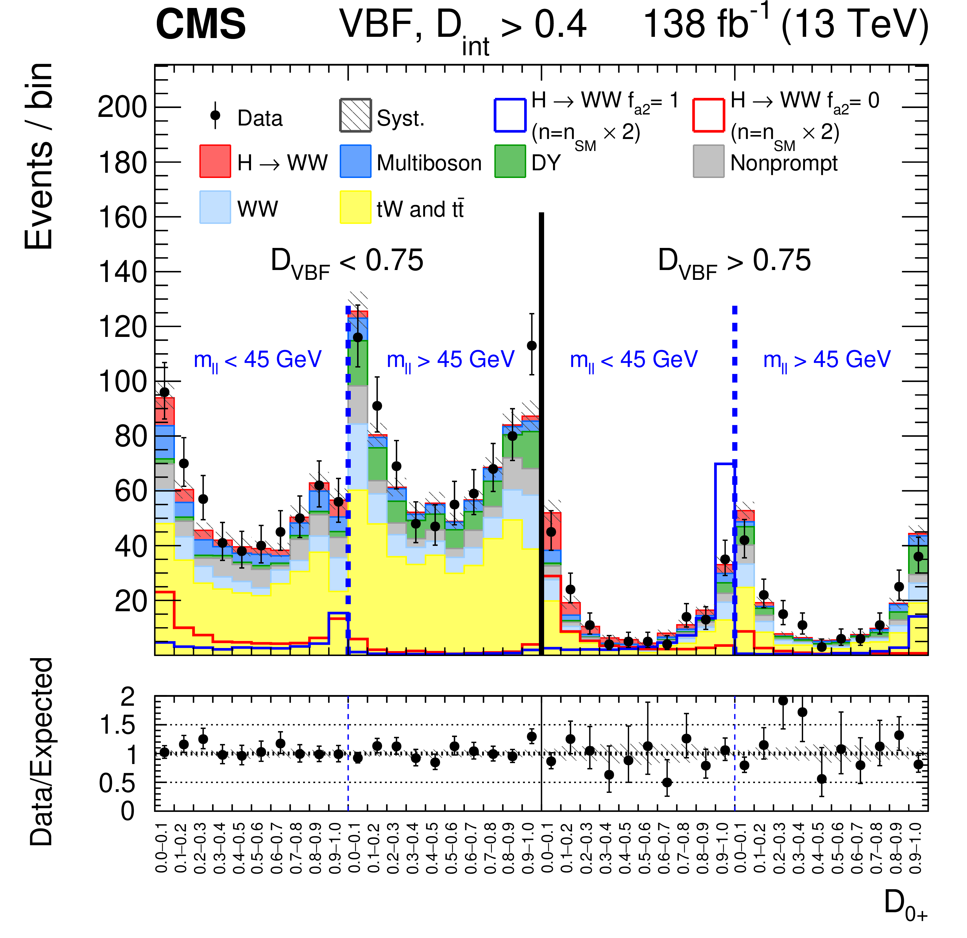
Figure 3-b:
Observed and predicted distributions after fitting the data for $ [\mathcal{D}_\text{VBF}, m_{\ell\ell}, \mathcal{D}_{0+}] $ in the VBF channel (upper), and for $ [m_{\ell\ell}, \mathcal{D}_{0+}] $ in the Resolved VH (lower left) and Boosted VH (lower right) channels. For the VBF channel, the $ \mathcal{D}_{\text{int}} < $ 0.4 (left) and $ \mathcal{D}_{\text{int}} > $ 0.4 (right) categories are shown. The predicted Higgs boson signal is shown stacked on top of the background distributions. For the fit, the $ a_{1} $ and $ a_2 $ HVV coupling contributions are included. The corresponding pure $ a_{1} $ ($ f_{a2} = $ 0) and $ a_2 $ ($ f_{a2} = $ 1) signal hypotheses are also shown superimposed, their yields correspond to the predicted number of SM signal events scaled by an arbitrary factor to improve visibility. The uncertainty band corresponds to the total systematic uncertainty. The lower panel in each figure shows the ratio of the number of events observed to the total prediction. |
png pdf |
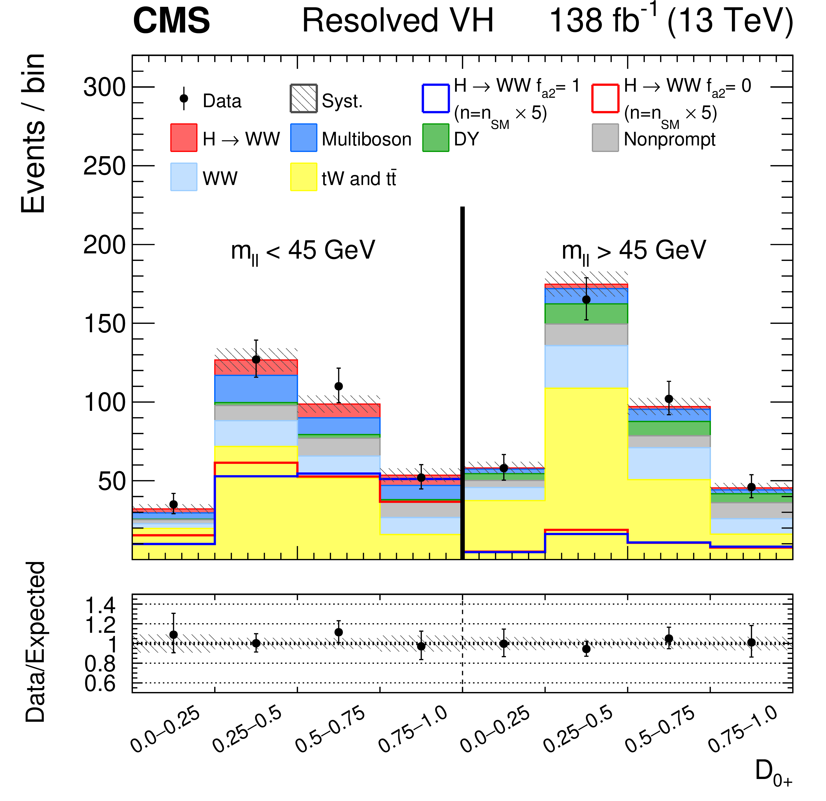
Figure 3-c:
Observed and predicted distributions after fitting the data for $ [\mathcal{D}_\text{VBF}, m_{\ell\ell}, \mathcal{D}_{0+}] $ in the VBF channel (upper), and for $ [m_{\ell\ell}, \mathcal{D}_{0+}] $ in the Resolved VH (lower left) and Boosted VH (lower right) channels. For the VBF channel, the $ \mathcal{D}_{\text{int}} < $ 0.4 (left) and $ \mathcal{D}_{\text{int}} > $ 0.4 (right) categories are shown. The predicted Higgs boson signal is shown stacked on top of the background distributions. For the fit, the $ a_{1} $ and $ a_2 $ HVV coupling contributions are included. The corresponding pure $ a_{1} $ ($ f_{a2} = $ 0) and $ a_2 $ ($ f_{a2} = $ 1) signal hypotheses are also shown superimposed, their yields correspond to the predicted number of SM signal events scaled by an arbitrary factor to improve visibility. The uncertainty band corresponds to the total systematic uncertainty. The lower panel in each figure shows the ratio of the number of events observed to the total prediction. |
png pdf |
Figure 3-d:
Observed and predicted distributions after fitting the data for $ [\mathcal{D}_\text{VBF}, m_{\ell\ell}, \mathcal{D}_{0+}] $ in the VBF channel (upper), and for $ [m_{\ell\ell}, \mathcal{D}_{0+}] $ in the Resolved VH (lower left) and Boosted VH (lower right) channels. For the VBF channel, the $ \mathcal{D}_{\text{int}} < $ 0.4 (left) and $ \mathcal{D}_{\text{int}} > $ 0.4 (right) categories are shown. The predicted Higgs boson signal is shown stacked on top of the background distributions. For the fit, the $ a_{1} $ and $ a_2 $ HVV coupling contributions are included. The corresponding pure $ a_{1} $ ($ f_{a2} = $ 0) and $ a_2 $ ($ f_{a2} = $ 1) signal hypotheses are also shown superimposed, their yields correspond to the predicted number of SM signal events scaled by an arbitrary factor to improve visibility. The uncertainty band corresponds to the total systematic uncertainty. The lower panel in each figure shows the ratio of the number of events observed to the total prediction. |
png pdf |
Figure 4:
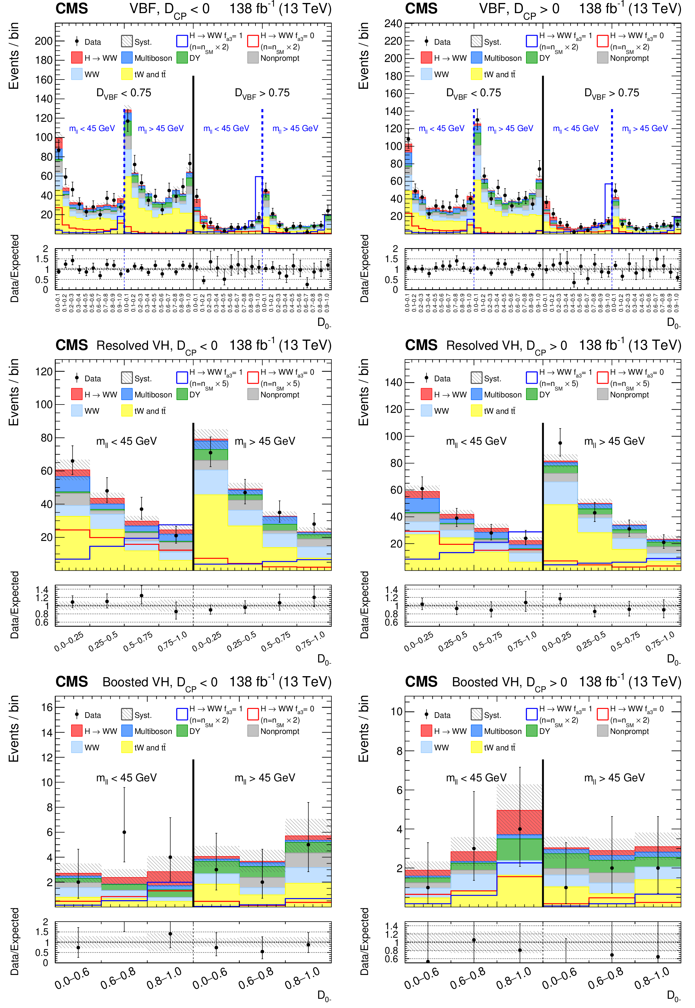
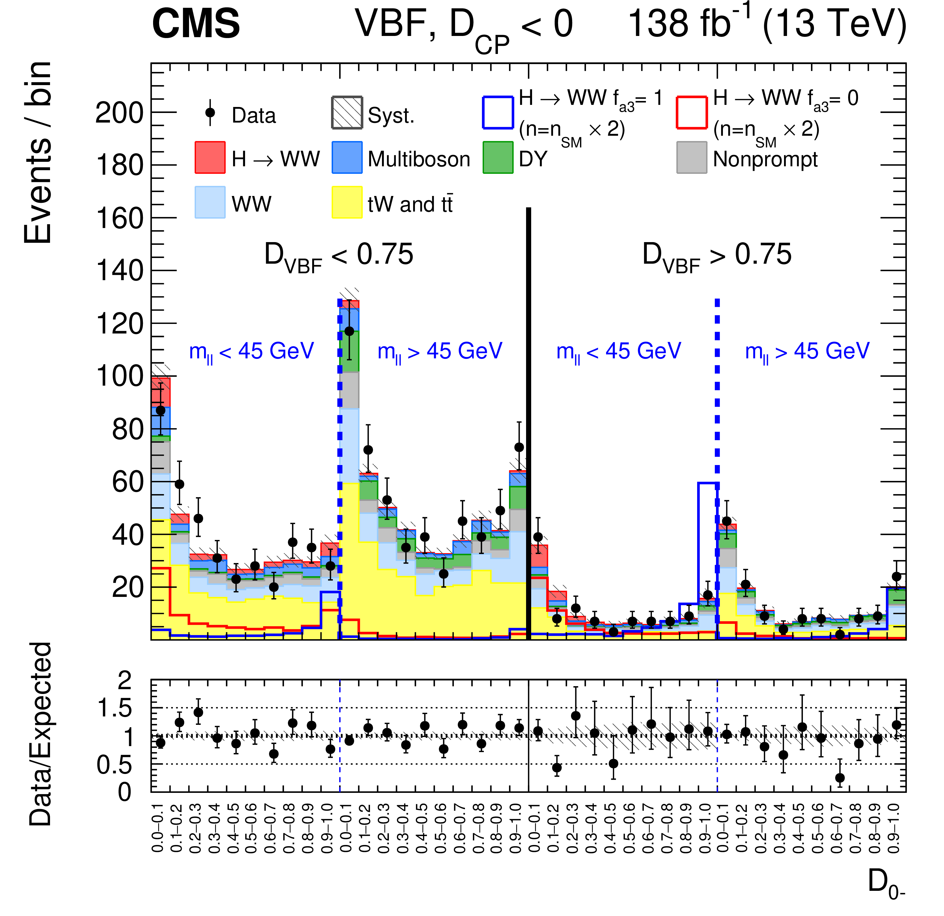
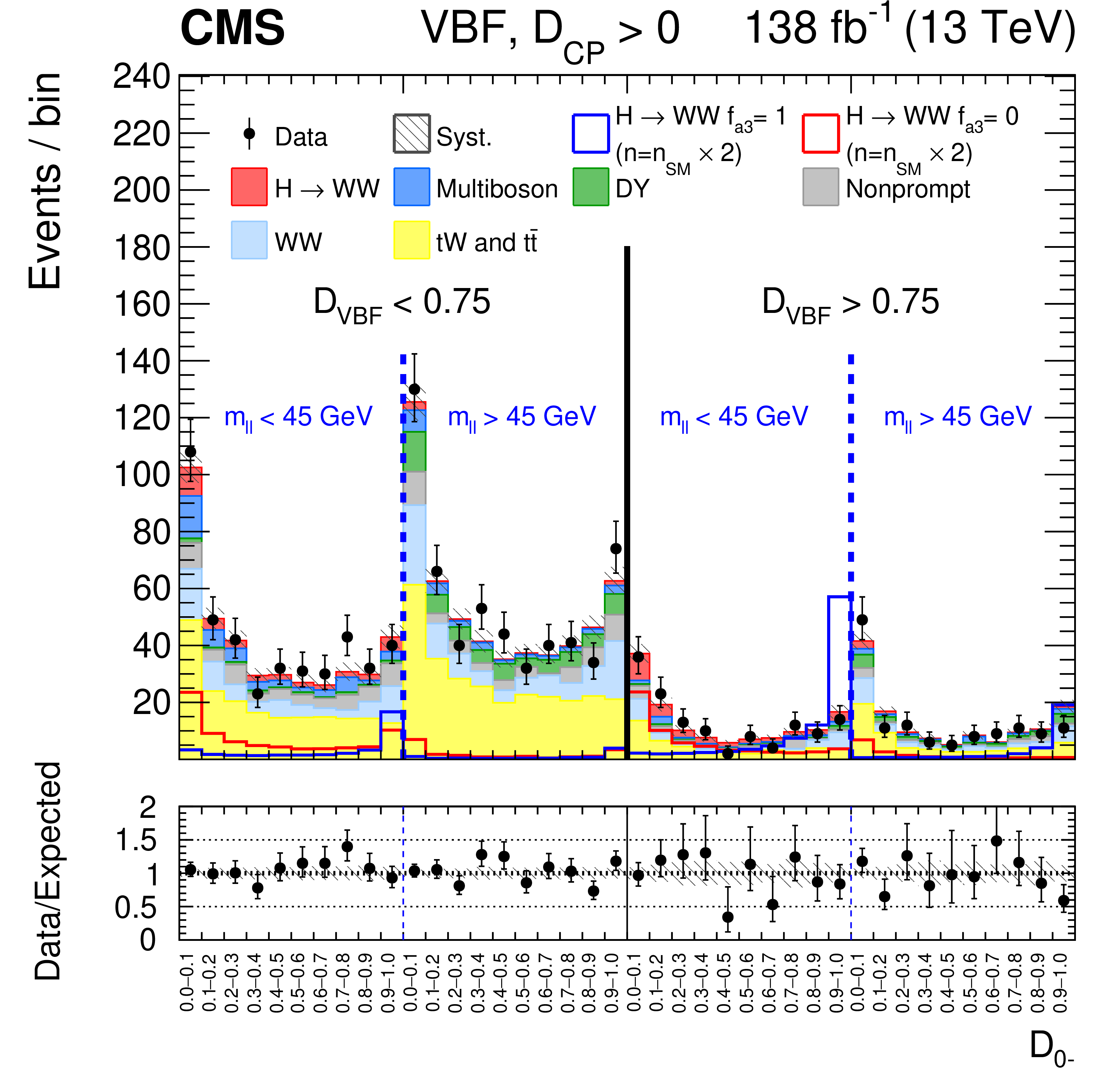
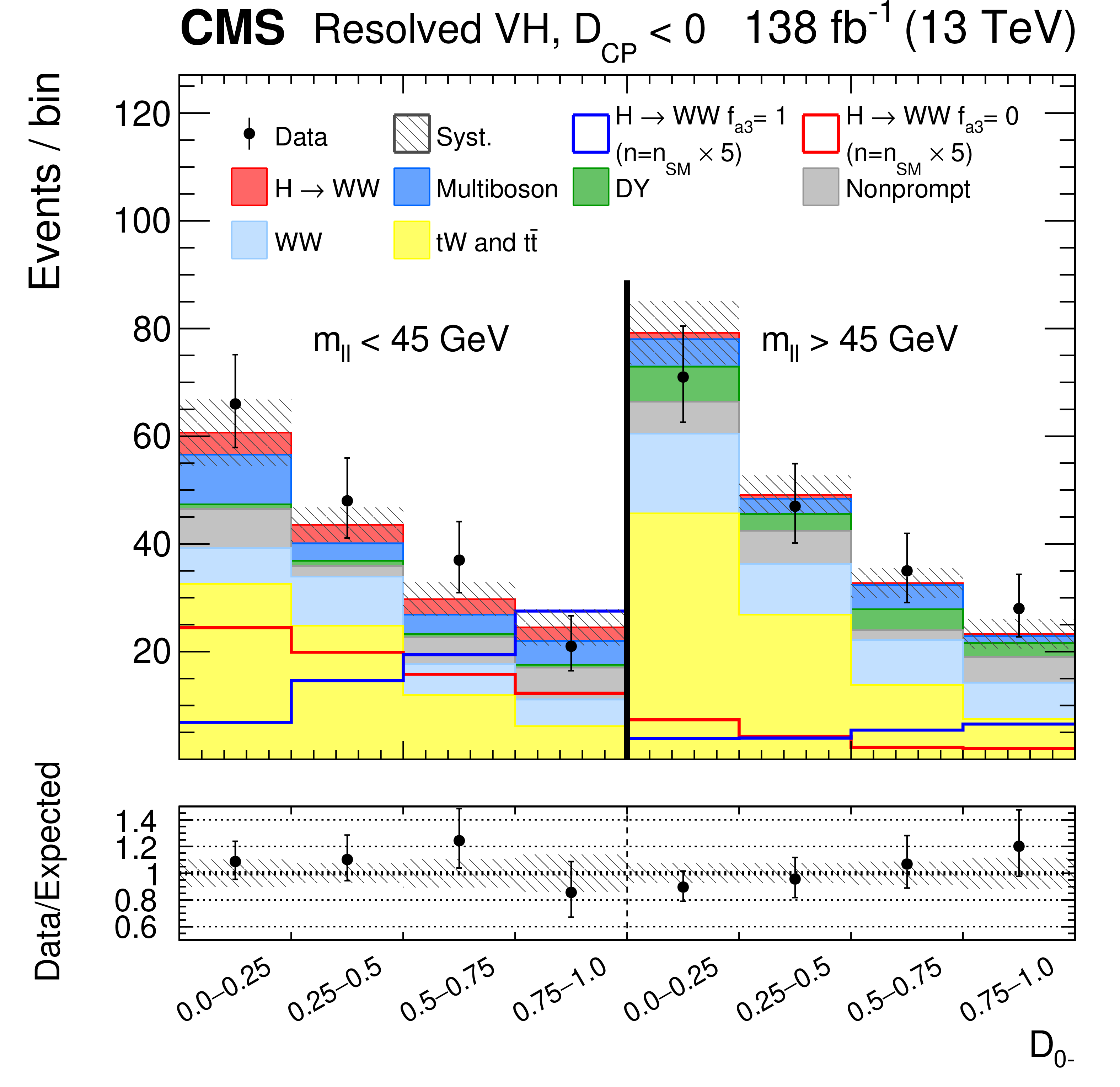
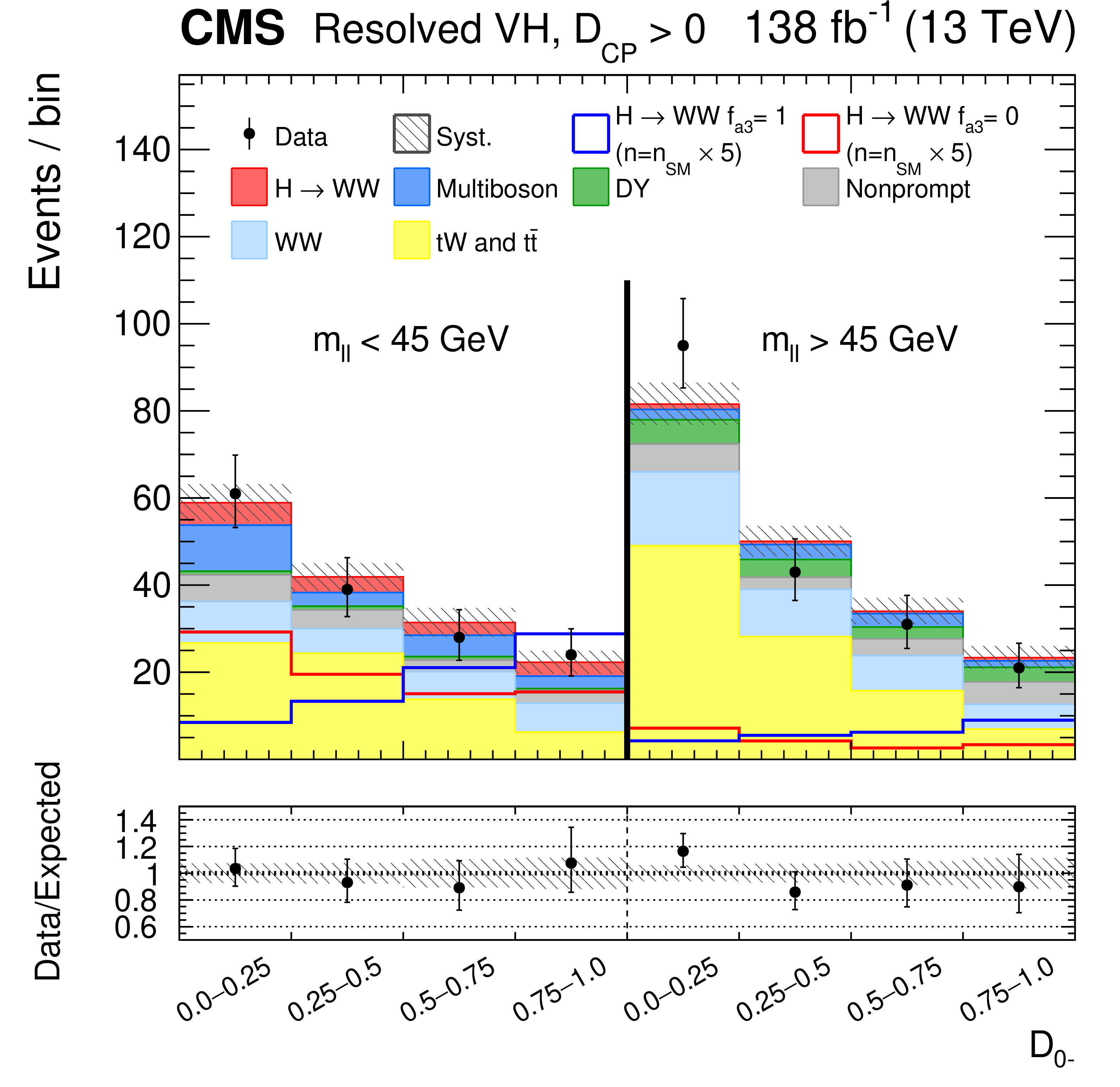
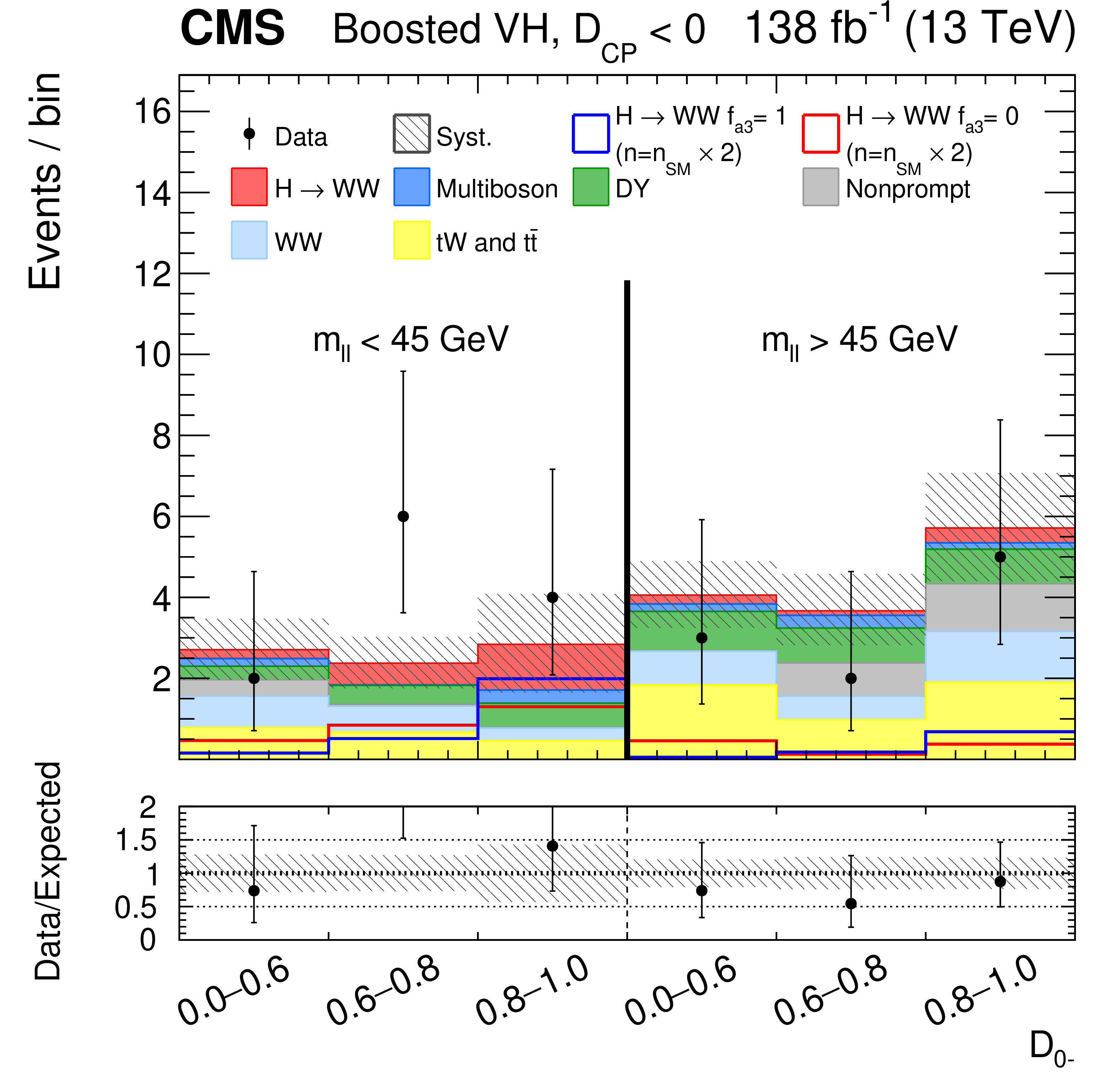
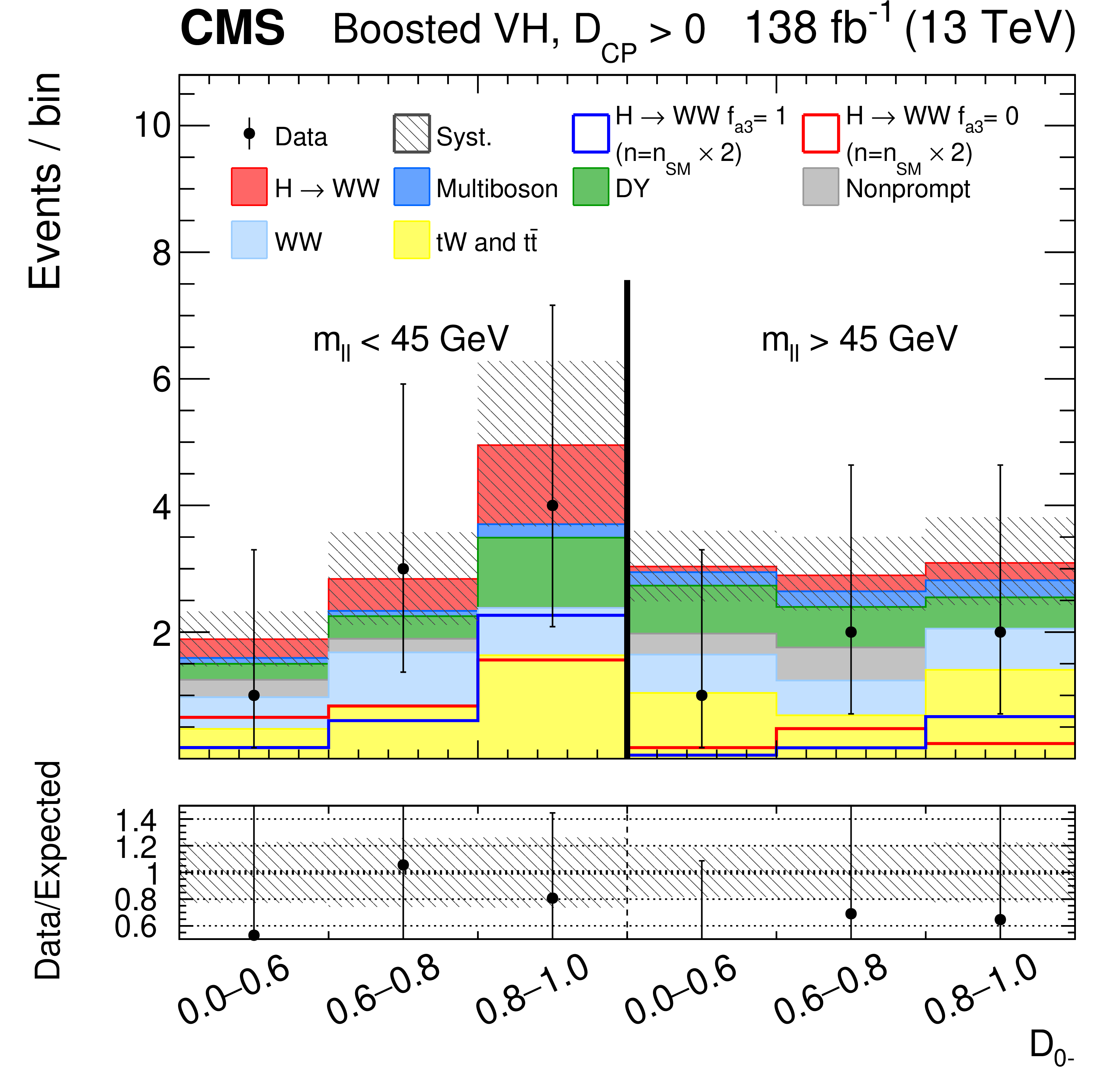
Observed and predicted distributions after fitting the data for $ [\mathcal{D}_\text{VBF}, m_{\ell\ell}, \mathcal{D}_{0-}] $ in the VBF channel (upper), and for $ [m_{\ell\ell}, \mathcal{D}_{0-}] $ in the Resolved VH (middle) and Boosted VH (lower) channels. For each channel, the $ \mathcal{D}_{CP} < $ 0 (left) and $ \mathcal{D}_{CP} > $ 0 (right) categories are shown. For the fit, the $ a_{1} $ and $ a_3 $ HVV coupling contributions are included. More details are given in the caption of Fig. 3. |
png pdf |
Figure 4-a:
Observed and predicted distributions after fitting the data for $ [\mathcal{D}_\text{VBF}, m_{\ell\ell}, \mathcal{D}_{0-}] $ in the VBF channel (upper), and for $ [m_{\ell\ell}, \mathcal{D}_{0-}] $ in the Resolved VH (middle) and Boosted VH (lower) channels. For each channel, the $ \mathcal{D}_{CP} < $ 0 (left) and $ \mathcal{D}_{CP} > $ 0 (right) categories are shown. For the fit, the $ a_{1} $ and $ a_3 $ HVV coupling contributions are included. More details are given in the caption of Fig. 3. |
png pdf |
Figure 4-b:
Observed and predicted distributions after fitting the data for $ [\mathcal{D}_\text{VBF}, m_{\ell\ell}, \mathcal{D}_{0-}] $ in the VBF channel (upper), and for $ [m_{\ell\ell}, \mathcal{D}_{0-}] $ in the Resolved VH (middle) and Boosted VH (lower) channels. For each channel, the $ \mathcal{D}_{CP} < $ 0 (left) and $ \mathcal{D}_{CP} > $ 0 (right) categories are shown. For the fit, the $ a_{1} $ and $ a_3 $ HVV coupling contributions are included. More details are given in the caption of Fig. 3. |
png pdf |
Figure 4-c:
Observed and predicted distributions after fitting the data for $ [\mathcal{D}_\text{VBF}, m_{\ell\ell}, \mathcal{D}_{0-}] $ in the VBF channel (upper), and for $ [m_{\ell\ell}, \mathcal{D}_{0-}] $ in the Resolved VH (middle) and Boosted VH (lower) channels. For each channel, the $ \mathcal{D}_{CP} < $ 0 (left) and $ \mathcal{D}_{CP} > $ 0 (right) categories are shown. For the fit, the $ a_{1} $ and $ a_3 $ HVV coupling contributions are included. More details are given in the caption of Fig. 3. |
png pdf |
Figure 4-d:
Observed and predicted distributions after fitting the data for $ [\mathcal{D}_\text{VBF}, m_{\ell\ell}, \mathcal{D}_{0-}] $ in the VBF channel (upper), and for $ [m_{\ell\ell}, \mathcal{D}_{0-}] $ in the Resolved VH (middle) and Boosted VH (lower) channels. For each channel, the $ \mathcal{D}_{CP} < $ 0 (left) and $ \mathcal{D}_{CP} > $ 0 (right) categories are shown. For the fit, the $ a_{1} $ and $ a_3 $ HVV coupling contributions are included. More details are given in the caption of Fig. 3. |
png pdf |
Figure 4-e:
Observed and predicted distributions after fitting the data for $ [\mathcal{D}_\text{VBF}, m_{\ell\ell}, \mathcal{D}_{0-}] $ in the VBF channel (upper), and for $ [m_{\ell\ell}, \mathcal{D}_{0-}] $ in the Resolved VH (middle) and Boosted VH (lower) channels. For each channel, the $ \mathcal{D}_{CP} < $ 0 (left) and $ \mathcal{D}_{CP} > $ 0 (right) categories are shown. For the fit, the $ a_{1} $ and $ a_3 $ HVV coupling contributions are included. More details are given in the caption of Fig. 3. |
png pdf |
Figure 4-f:
Observed and predicted distributions after fitting the data for $ [\mathcal{D}_\text{VBF}, m_{\ell\ell}, \mathcal{D}_{0-}] $ in the VBF channel (upper), and for $ [m_{\ell\ell}, \mathcal{D}_{0-}] $ in the Resolved VH (middle) and Boosted VH (lower) channels. For each channel, the $ \mathcal{D}_{CP} < $ 0 (left) and $ \mathcal{D}_{CP} > $ 0 (right) categories are shown. For the fit, the $ a_{1} $ and $ a_3 $ HVV coupling contributions are included. More details are given in the caption of Fig. 3. |
png pdf |
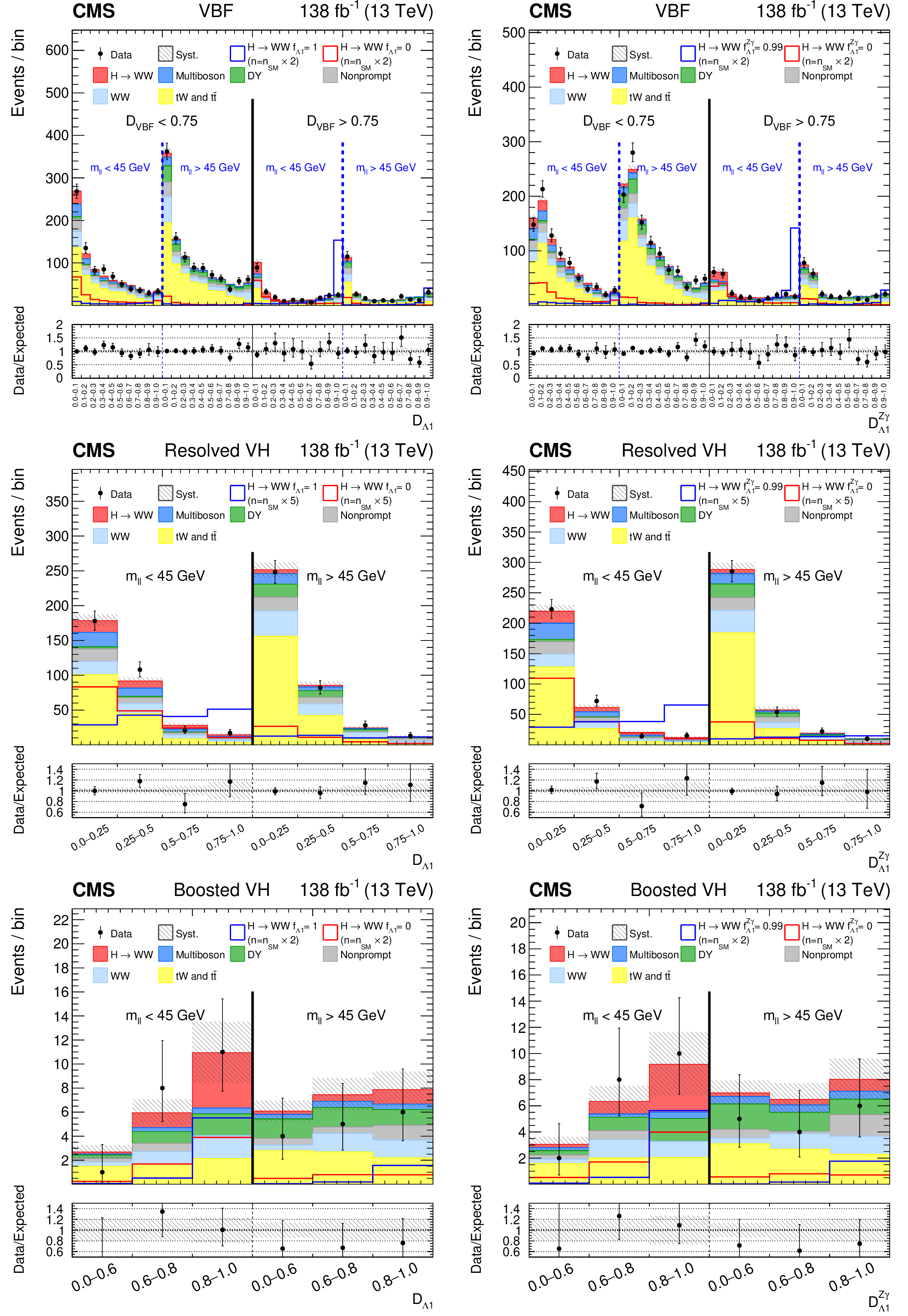
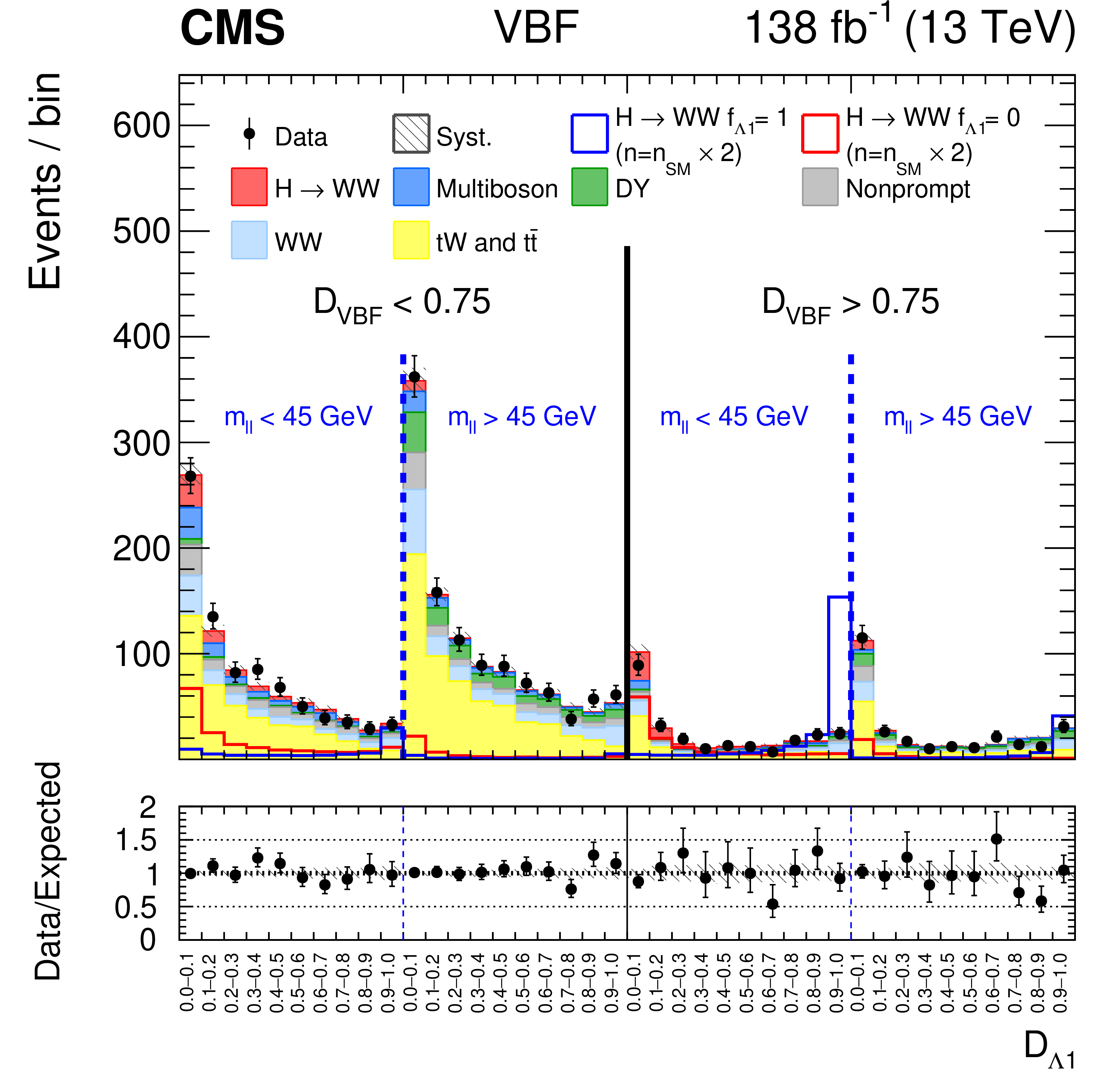
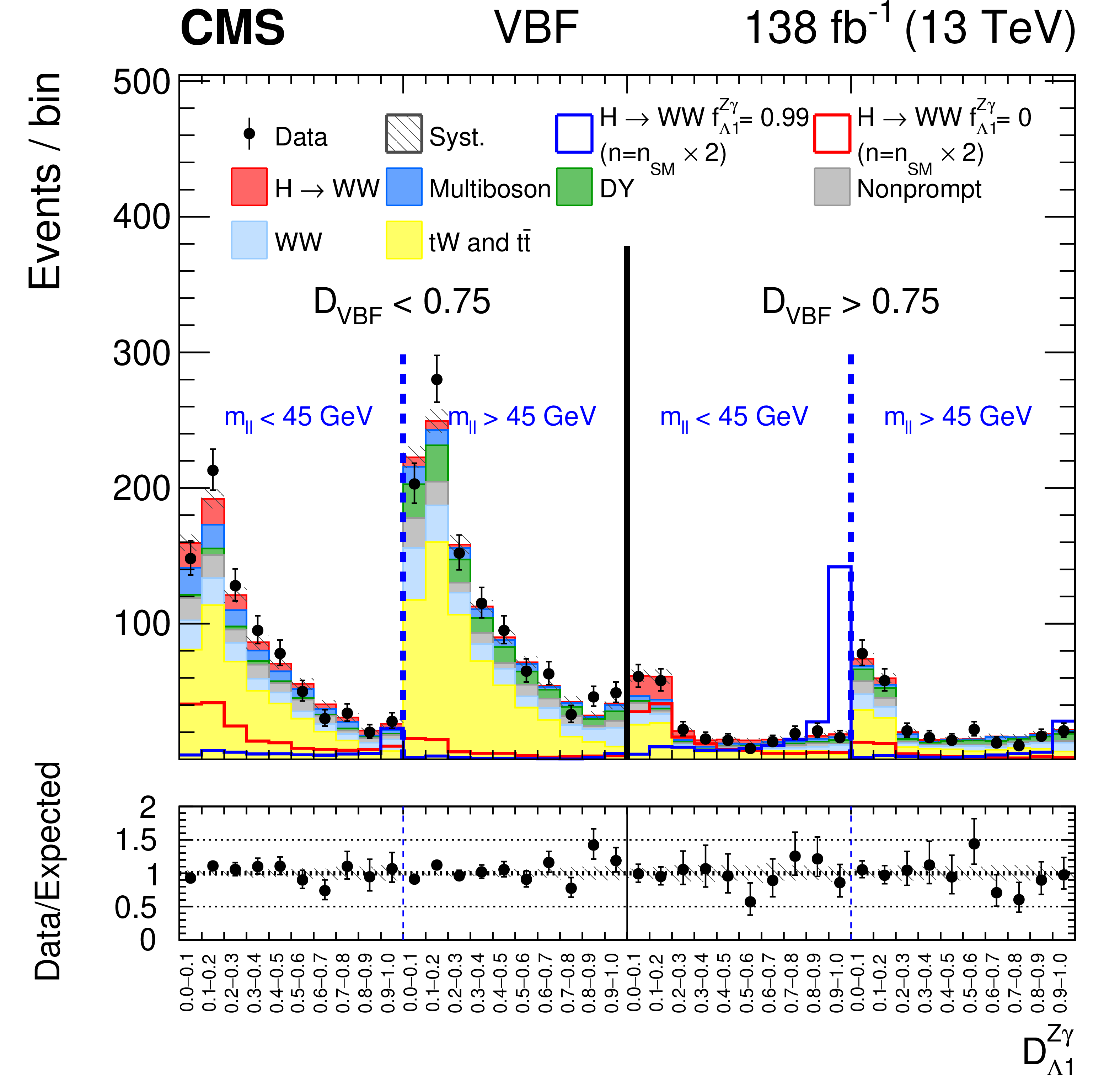
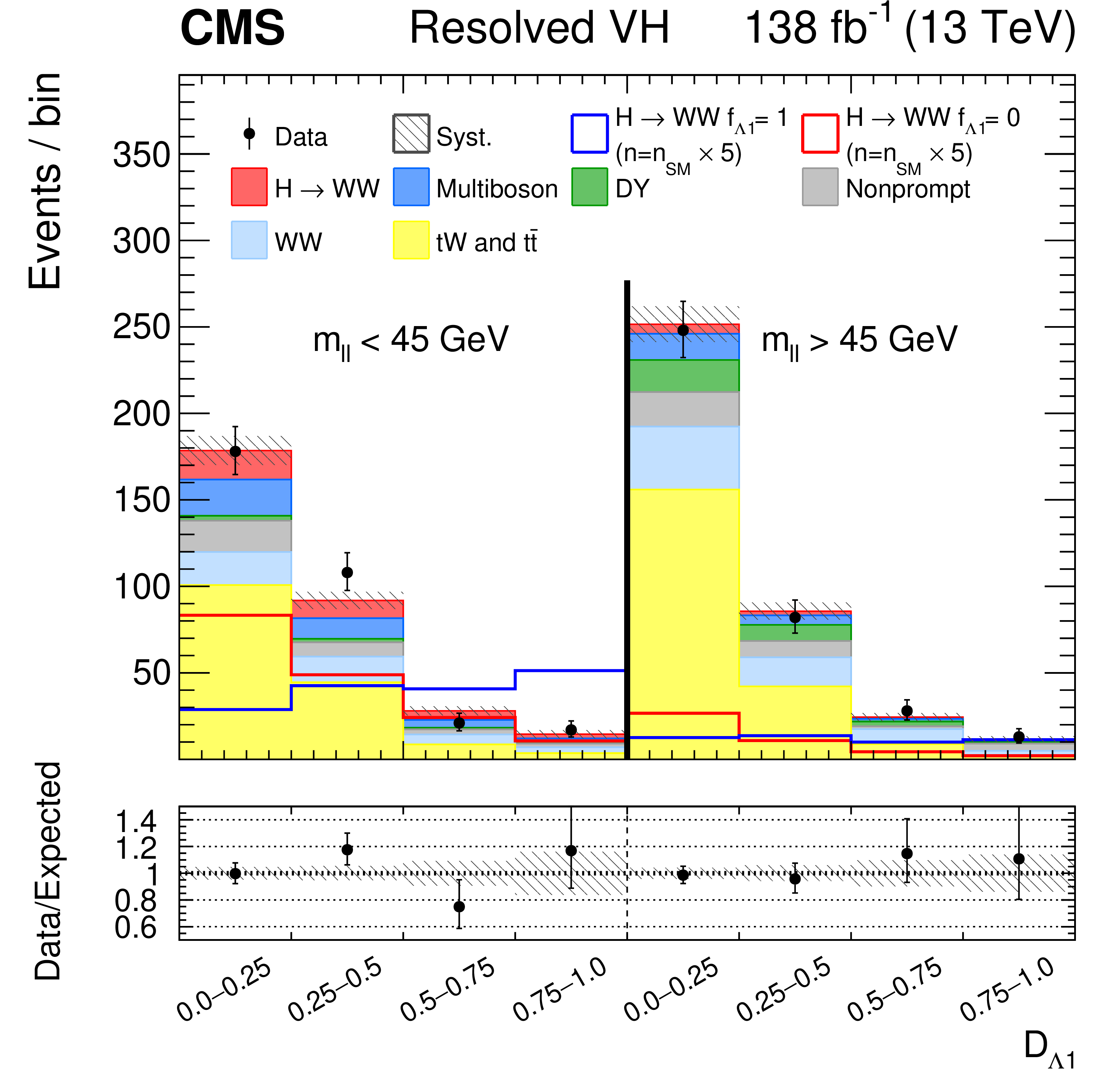
Figure 5:
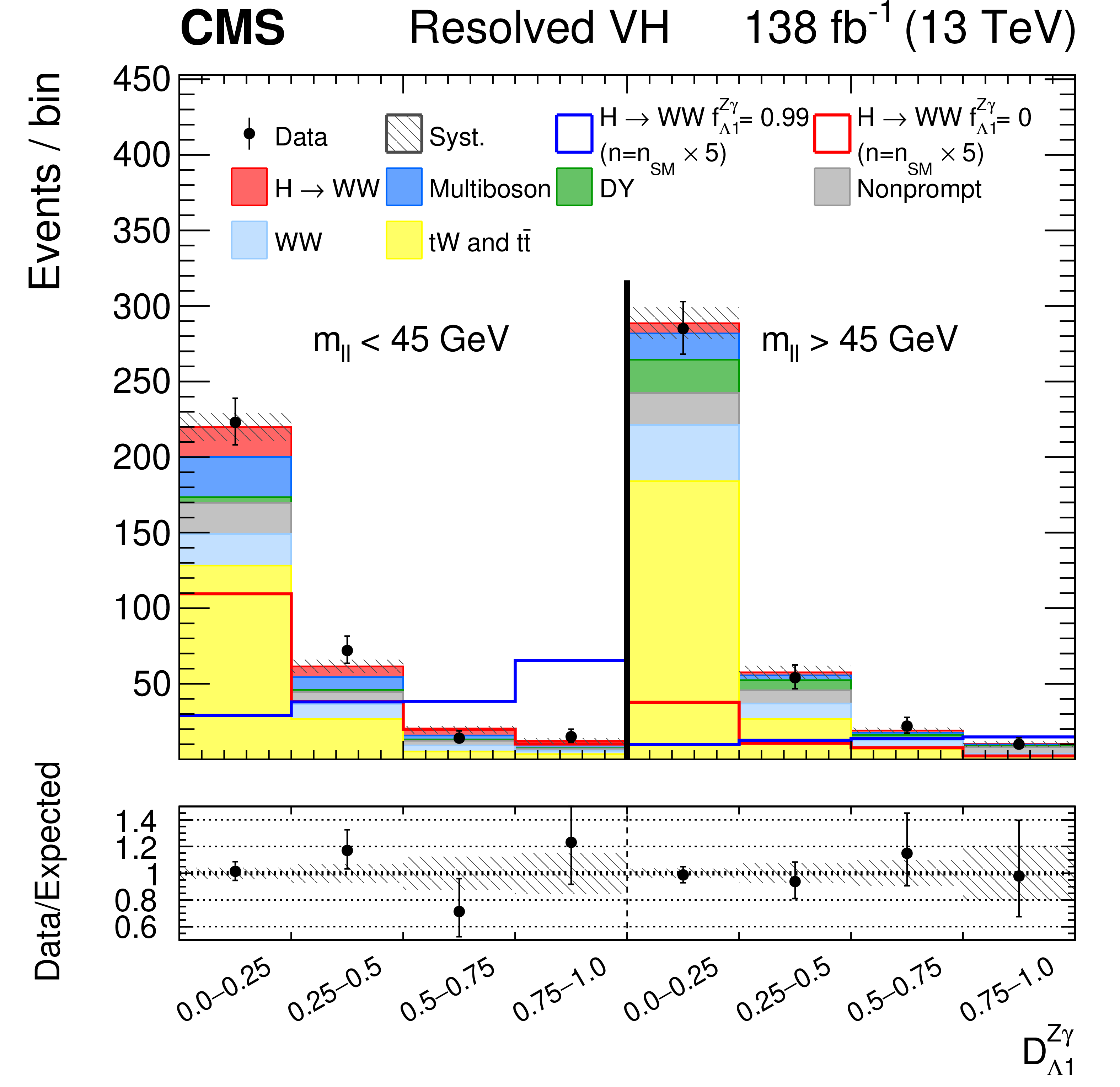
Observed and predicted distributions after fitting the data for $ [\mathcal{D}_\text{VBF}, m_{\ell\ell}, \mathcal{D}_{\Lambda 1}] $ (upper left) and $ [\mathcal{D}_\text{VBF}, m_{\ell\ell}, \mathcal{D}_{\Lambda 1}^{\mathrm{Z}\gamma}] $ (upper right) in the VBF channel, and for $ [m_{\ell\ell}, \mathcal{D}_{\Lambda 1}] $ (left) and $ [m_{\ell\ell}, \mathcal{D}_{\Lambda 1}^{\mathrm{Z}\gamma}] $ (right) in the Resolved VH (middle) and Boosted VH (lower) channels. For the fits, the $ a_{1} $ and $ \kappa_1/(\Lambda_1)^2 $ (left) or $ a_{1} $ and $ \kappa_2^{\mathrm{Z}\gamma}/(\Lambda_1^{\mathrm{Z}\gamma})^2 $ (right) HVV coupling contributions are included. More details are given in the caption of Fig. 3. |
png pdf |
Figure 5-a:
Observed and predicted distributions after fitting the data for $ [\mathcal{D}_\text{VBF}, m_{\ell\ell}, \mathcal{D}_{\Lambda 1}] $ (upper left) and $ [\mathcal{D}_\text{VBF}, m_{\ell\ell}, \mathcal{D}_{\Lambda 1}^{\mathrm{Z}\gamma}] $ (upper right) in the VBF channel, and for $ [m_{\ell\ell}, \mathcal{D}_{\Lambda 1}] $ (left) and $ [m_{\ell\ell}, \mathcal{D}_{\Lambda 1}^{\mathrm{Z}\gamma}] $ (right) in the Resolved VH (middle) and Boosted VH (lower) channels. For the fits, the $ a_{1} $ and $ \kappa_1/(\Lambda_1)^2 $ (left) or $ a_{1} $ and $ \kappa_2^{\mathrm{Z}\gamma}/(\Lambda_1^{\mathrm{Z}\gamma})^2 $ (right) HVV coupling contributions are included. More details are given in the caption of Fig. 3. |
png pdf |
Figure 5-b:
Observed and predicted distributions after fitting the data for $ [\mathcal{D}_\text{VBF}, m_{\ell\ell}, \mathcal{D}_{\Lambda 1}] $ (upper left) and $ [\mathcal{D}_\text{VBF}, m_{\ell\ell}, \mathcal{D}_{\Lambda 1}^{\mathrm{Z}\gamma}] $ (upper right) in the VBF channel, and for $ [m_{\ell\ell}, \mathcal{D}_{\Lambda 1}] $ (left) and $ [m_{\ell\ell}, \mathcal{D}_{\Lambda 1}^{\mathrm{Z}\gamma}] $ (right) in the Resolved VH (middle) and Boosted VH (lower) channels. For the fits, the $ a_{1} $ and $ \kappa_1/(\Lambda_1)^2 $ (left) or $ a_{1} $ and $ \kappa_2^{\mathrm{Z}\gamma}/(\Lambda_1^{\mathrm{Z}\gamma})^2 $ (right) HVV coupling contributions are included. More details are given in the caption of Fig. 3. |
png pdf |
Figure 5-c:
Observed and predicted distributions after fitting the data for $ [\mathcal{D}_\text{VBF}, m_{\ell\ell}, \mathcal{D}_{\Lambda 1}] $ (upper left) and $ [\mathcal{D}_\text{VBF}, m_{\ell\ell}, \mathcal{D}_{\Lambda 1}^{\mathrm{Z}\gamma}] $ (upper right) in the VBF channel, and for $ [m_{\ell\ell}, \mathcal{D}_{\Lambda 1}] $ (left) and $ [m_{\ell\ell}, \mathcal{D}_{\Lambda 1}^{\mathrm{Z}\gamma}] $ (right) in the Resolved VH (middle) and Boosted VH (lower) channels. For the fits, the $ a_{1} $ and $ \kappa_1/(\Lambda_1)^2 $ (left) or $ a_{1} $ and $ \kappa_2^{\mathrm{Z}\gamma}/(\Lambda_1^{\mathrm{Z}\gamma})^2 $ (right) HVV coupling contributions are included. More details are given in the caption of Fig. 3. |
png pdf |
Figure 5-d:
Observed and predicted distributions after fitting the data for $ [\mathcal{D}_\text{VBF}, m_{\ell\ell}, \mathcal{D}_{\Lambda 1}] $ (upper left) and $ [\mathcal{D}_\text{VBF}, m_{\ell\ell}, \mathcal{D}_{\Lambda 1}^{\mathrm{Z}\gamma}] $ (upper right) in the VBF channel, and for $ [m_{\ell\ell}, \mathcal{D}_{\Lambda 1}] $ (left) and $ [m_{\ell\ell}, \mathcal{D}_{\Lambda 1}^{\mathrm{Z}\gamma}] $ (right) in the Resolved VH (middle) and Boosted VH (lower) channels. For the fits, the $ a_{1} $ and $ \kappa_1/(\Lambda_1)^2 $ (left) or $ a_{1} $ and $ \kappa_2^{\mathrm{Z}\gamma}/(\Lambda_1^{\mathrm{Z}\gamma})^2 $ (right) HVV coupling contributions are included. More details are given in the caption of Fig. 3. |

png pdf |
Figure 5-e:
Observed and predicted distributions after fitting the data for $ [\mathcal{D}_\text{VBF}, m_{\ell\ell}, \mathcal{D}_{\Lambda 1}] $ (upper left) and $ [\mathcal{D}_\text{VBF}, m_{\ell\ell}, \mathcal{D}_{\Lambda 1}^{\mathrm{Z}\gamma}] $ (upper right) in the VBF channel, and for $ [m_{\ell\ell}, \mathcal{D}_{\Lambda 1}] $ (left) and $ [m_{\ell\ell}, \mathcal{D}_{\Lambda 1}^{\mathrm{Z}\gamma}] $ (right) in the Resolved VH (middle) and Boosted VH (lower) channels. For the fits, the $ a_{1} $ and $ \kappa_1/(\Lambda_1)^2 $ (left) or $ a_{1} $ and $ \kappa_2^{\mathrm{Z}\gamma}/(\Lambda_1^{\mathrm{Z}\gamma})^2 $ (right) HVV coupling contributions are included. More details are given in the caption of Fig. 3. |
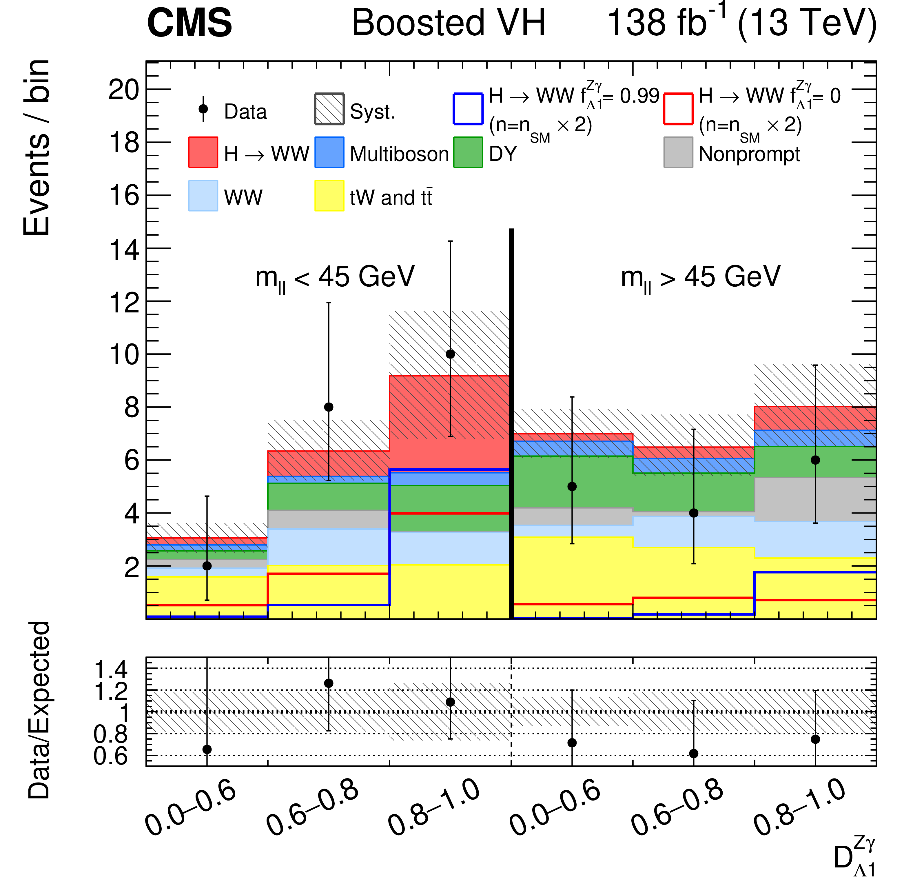
png pdf |
Figure 5-f:
Observed and predicted distributions after fitting the data for $ [\mathcal{D}_\text{VBF}, m_{\ell\ell}, \mathcal{D}_{\Lambda 1}] $ (upper left) and $ [\mathcal{D}_\text{VBF}, m_{\ell\ell}, \mathcal{D}_{\Lambda 1}^{\mathrm{Z}\gamma}] $ (upper right) in the VBF channel, and for $ [m_{\ell\ell}, \mathcal{D}_{\Lambda 1}] $ (left) and $ [m_{\ell\ell}, \mathcal{D}_{\Lambda 1}^{\mathrm{Z}\gamma}] $ (right) in the Resolved VH (middle) and Boosted VH (lower) channels. For the fits, the $ a_{1} $ and $ \kappa_1/(\Lambda_1)^2 $ (left) or $ a_{1} $ and $ \kappa_2^{\mathrm{Z}\gamma}/(\Lambda_1^{\mathrm{Z}\gamma})^2 $ (right) HVV coupling contributions are included. More details are given in the caption of Fig. 3. |
png pdf |
Figure 6:
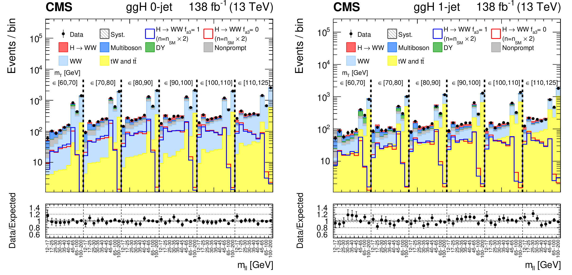
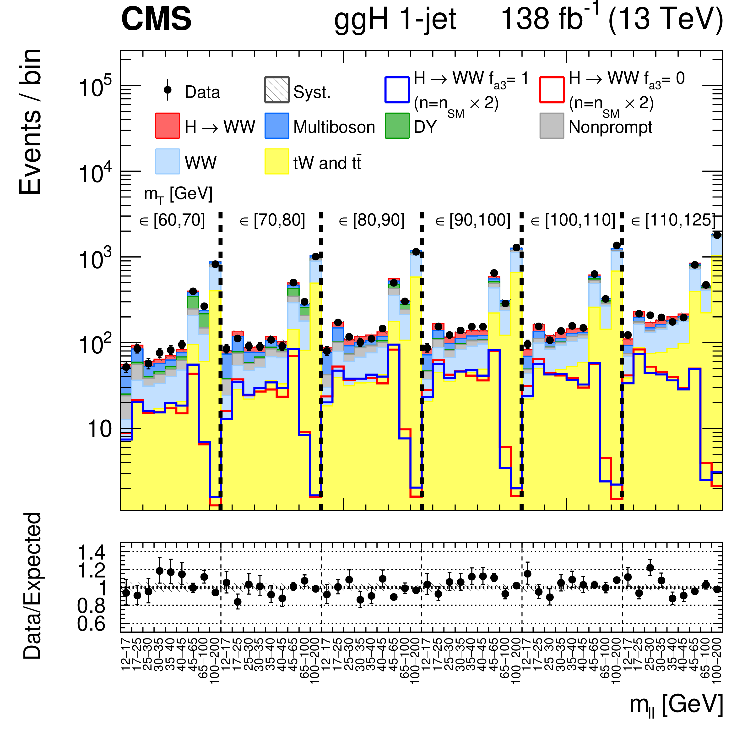
Observed and predicted distributions after fitting the data for $ [m_{\mathrm{T}}, m_{\ell\ell}] $ in the 0- (left) and 1-jet (right) ggH channels. For the fit, the $ a_{1} $ and $ a_3 \mathrm{H}\mathrm{V}\mathrm{V} $ coupling contributions are included. More details are given in the caption of Fig. 3. |

png pdf |
Figure 6-a:
Observed and predicted distributions after fitting the data for $ [m_{\mathrm{T}}, m_{\ell\ell}] $ in the 0- (left) and 1-jet (right) ggH channels. For the fit, the $ a_{1} $ and $ a_3 \mathrm{H}\mathrm{V}\mathrm{V} $ coupling contributions are included. More details are given in the caption of Fig. 3. |
png pdf |
Figure 6-b:
Observed and predicted distributions after fitting the data for $ [m_{\mathrm{T}}, m_{\ell\ell}] $ in the 0- (left) and 1-jet (right) ggH channels. For the fit, the $ a_{1} $ and $ a_3 \mathrm{H}\mathrm{V}\mathrm{V} $ coupling contributions are included. More details are given in the caption of Fig. 3. |
png pdf |
Figure 7:
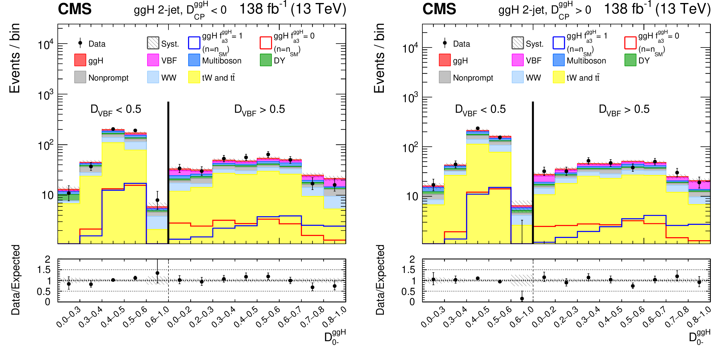
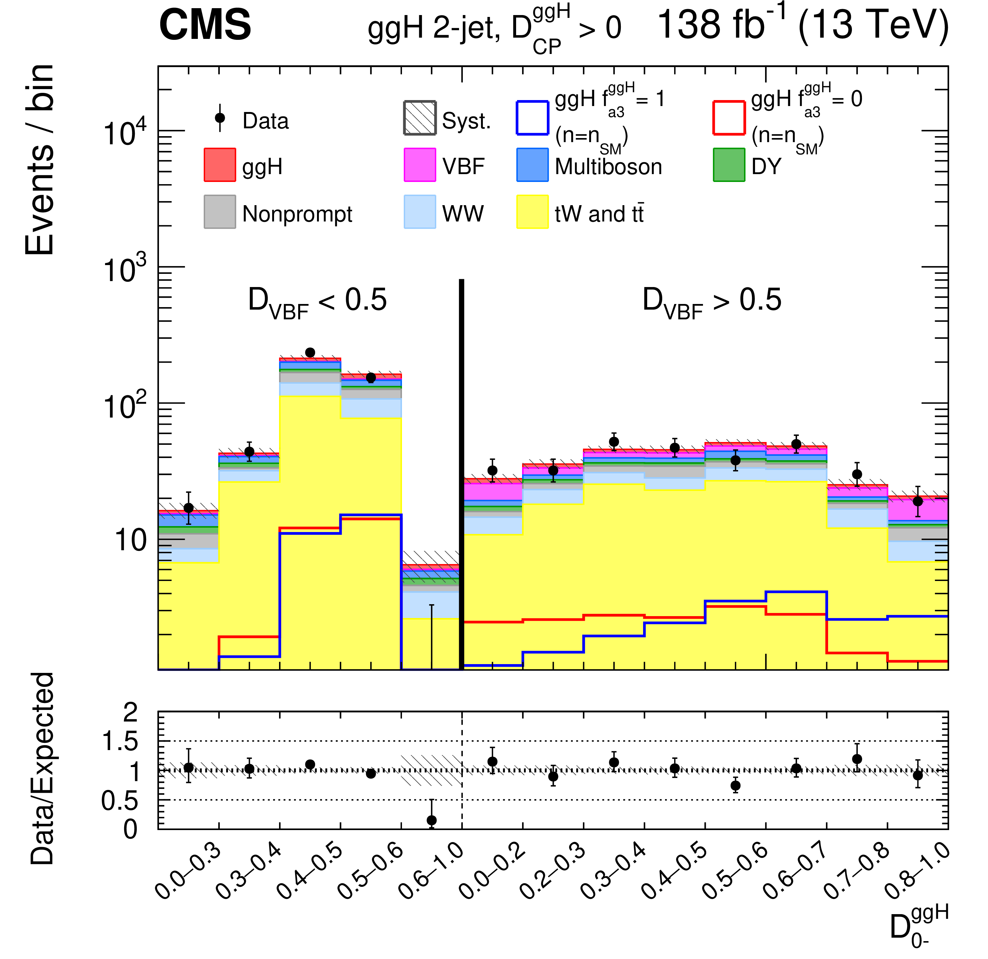
Observed and predicted distributions after fitting the data for $ [\mathcal{D}_\text{VBF} $, $ \mathcal{D}^{\mathrm{g}\mathrm{g}\mathrm{H}}_{0-}] $ in the 2-jet ggH channel. Both the $ \mathcal{D}^{\mathrm{g}\mathrm{g}\mathrm{H}}_{\text{CP}} < $ 0 (left) and $ \mathcal{D}^{\mathrm{g}\mathrm{g}\mathrm{H}}_{\text{CP}} > $ 0 (right) categories are shown. In this case, the VBF and ggH signals are shown separately. For the fit, the $ a_2^{\mathrm{g}\mathrm{g}} $ and $ a_3^{\mathrm{g}\mathrm{g}} $ coupling contributions are included. The corresponding pure $ a_2^{\mathrm{g}\mathrm{g}} $ ($ f_{a3}^{\mathrm{g}\mathrm{g}\mathrm{H}} = $ 0) and $ a_3^{\mathrm{g}\mathrm{g}} $ ($ f_{a3}^{\mathrm{g}\mathrm{g}\mathrm{H}} = $ 1) signal hypotheses are also shown superimposed, their yields correspond to the predicted number of SM signal events. More details are given in the caption of Fig. 3. |

png pdf |
Figure 7-a:
Observed and predicted distributions after fitting the data for $ [\mathcal{D}_\text{VBF} $, $ \mathcal{D}^{\mathrm{g}\mathrm{g}\mathrm{H}}_{0-}] $ in the 2-jet ggH channel. Both the $ \mathcal{D}^{\mathrm{g}\mathrm{g}\mathrm{H}}_{\text{CP}} < $ 0 (left) and $ \mathcal{D}^{\mathrm{g}\mathrm{g}\mathrm{H}}_{\text{CP}} > $ 0 (right) categories are shown. In this case, the VBF and ggH signals are shown separately. For the fit, the $ a_2^{\mathrm{g}\mathrm{g}} $ and $ a_3^{\mathrm{g}\mathrm{g}} $ coupling contributions are included. The corresponding pure $ a_2^{\mathrm{g}\mathrm{g}} $ ($ f_{a3}^{\mathrm{g}\mathrm{g}\mathrm{H}} = $ 0) and $ a_3^{\mathrm{g}\mathrm{g}} $ ($ f_{a3}^{\mathrm{g}\mathrm{g}\mathrm{H}} = $ 1) signal hypotheses are also shown superimposed, their yields correspond to the predicted number of SM signal events. More details are given in the caption of Fig. 3. |
png pdf |
Figure 7-b:
Observed and predicted distributions after fitting the data for $ [\mathcal{D}_\text{VBF} $, $ \mathcal{D}^{\mathrm{g}\mathrm{g}\mathrm{H}}_{0-}] $ in the 2-jet ggH channel. Both the $ \mathcal{D}^{\mathrm{g}\mathrm{g}\mathrm{H}}_{\text{CP}} < $ 0 (left) and $ \mathcal{D}^{\mathrm{g}\mathrm{g}\mathrm{H}}_{\text{CP}} > $ 0 (right) categories are shown. In this case, the VBF and ggH signals are shown separately. For the fit, the $ a_2^{\mathrm{g}\mathrm{g}} $ and $ a_3^{\mathrm{g}\mathrm{g}} $ coupling contributions are included. The corresponding pure $ a_2^{\mathrm{g}\mathrm{g}} $ ($ f_{a3}^{\mathrm{g}\mathrm{g}\mathrm{H}} = $ 0) and $ a_3^{\mathrm{g}\mathrm{g}} $ ($ f_{a3}^{\mathrm{g}\mathrm{g}\mathrm{H}} = $ 1) signal hypotheses are also shown superimposed, their yields correspond to the predicted number of SM signal events. More details are given in the caption of Fig. 3. |
png pdf |
Figure 8:
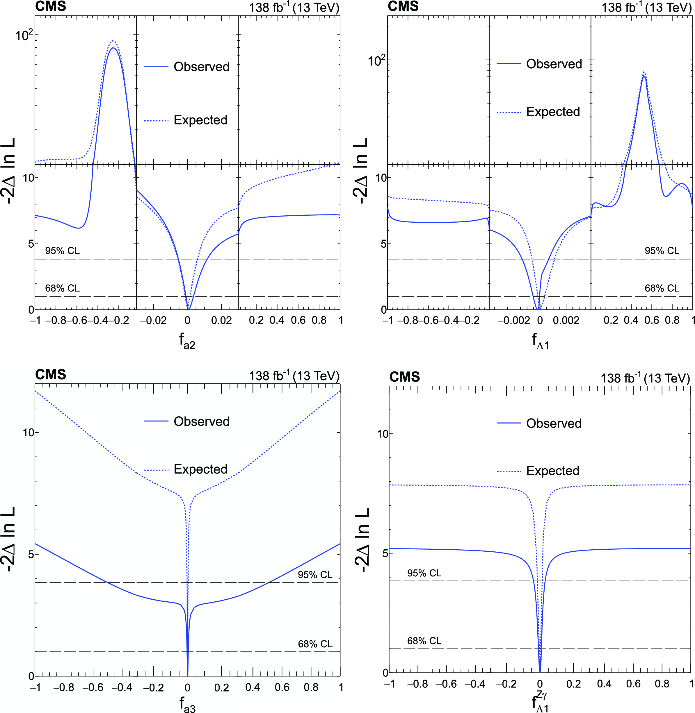
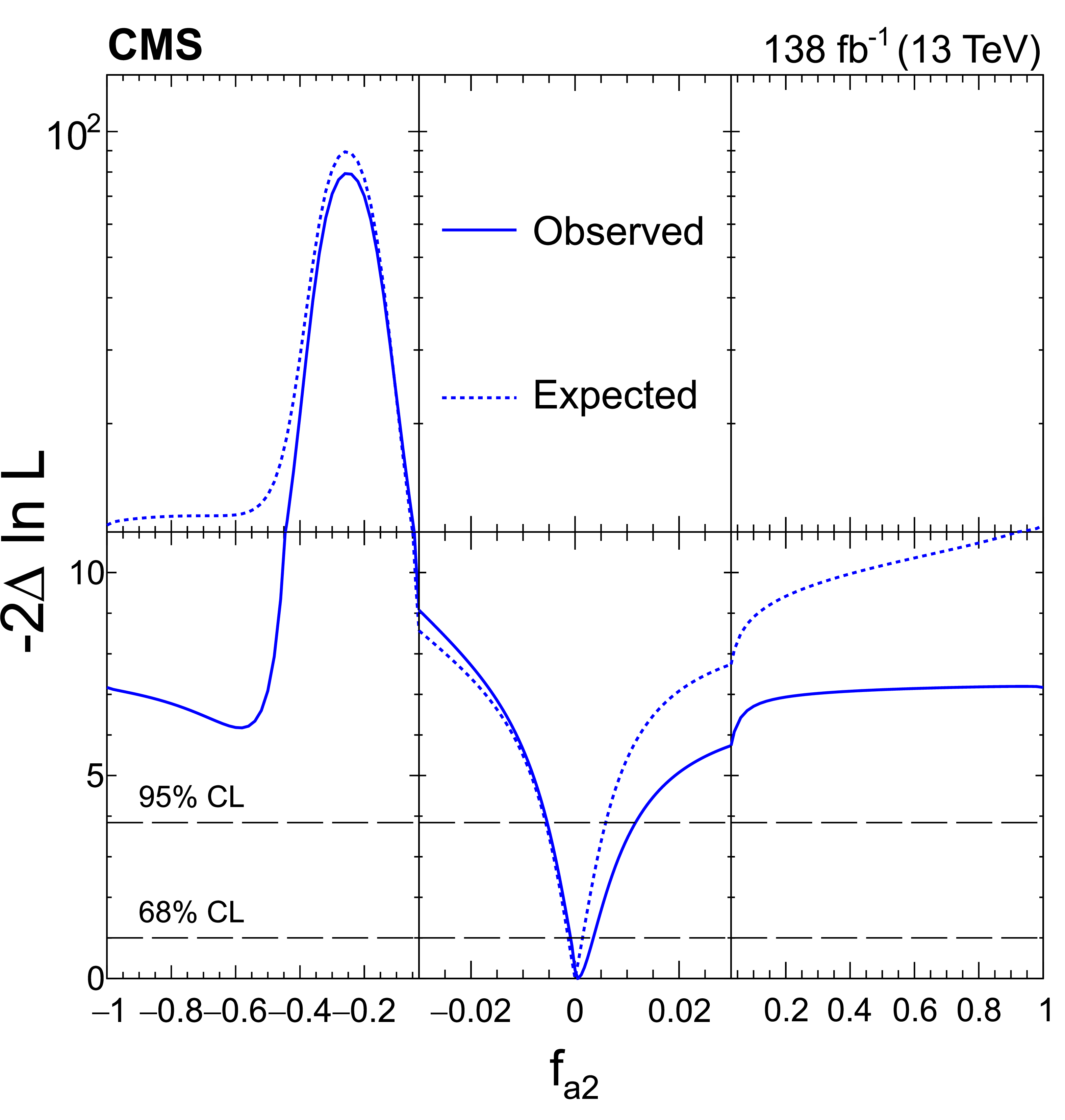
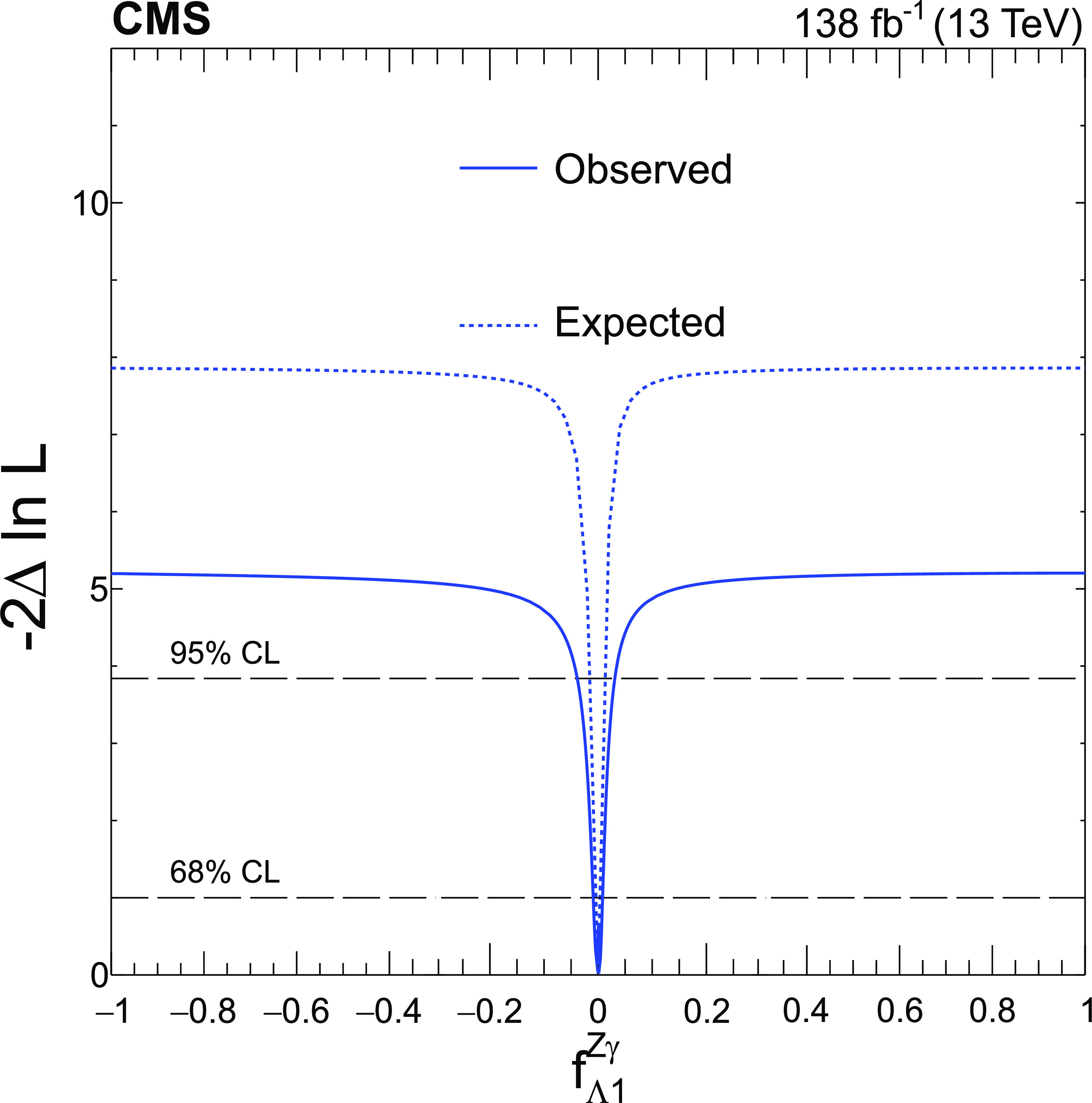
Expected (dashed) and observed (solid) profiled likelihood on $ f_{a2} $ (upper left), $ f_{\Lambda 1} $ (upper right), $ f_{a3} $ (lower left), and $ f_{\Lambda 1}^{\mathrm{Z}\gamma} $ (lower right) using Approach 1. In each case, the signal strength modifiers are treated as free parameters. The dashed horizontal lines show the 68 and 95% CL regions. Axis scales are varied for $ f_{a2} $ and $ f_{\Lambda 1} $ to improve the visibility of important features. |
png pdf |
Figure 8-a:
Expected (dashed) and observed (solid) profiled likelihood on $ f_{a2} $ (upper left), $ f_{\Lambda 1} $ (upper right), $ f_{a3} $ (lower left), and $ f_{\Lambda 1}^{\mathrm{Z}\gamma} $ (lower right) using Approach 1. In each case, the signal strength modifiers are treated as free parameters. The dashed horizontal lines show the 68 and 95% CL regions. Axis scales are varied for $ f_{a2} $ and $ f_{\Lambda 1} $ to improve the visibility of important features. |

png pdf |
Figure 8-b:
Expected (dashed) and observed (solid) profiled likelihood on $ f_{a2} $ (upper left), $ f_{\Lambda 1} $ (upper right), $ f_{a3} $ (lower left), and $ f_{\Lambda 1}^{\mathrm{Z}\gamma} $ (lower right) using Approach 1. In each case, the signal strength modifiers are treated as free parameters. The dashed horizontal lines show the 68 and 95% CL regions. Axis scales are varied for $ f_{a2} $ and $ f_{\Lambda 1} $ to improve the visibility of important features. |

png pdf |
Figure 8-c:
Expected (dashed) and observed (solid) profiled likelihood on $ f_{a2} $ (upper left), $ f_{\Lambda 1} $ (upper right), $ f_{a3} $ (lower left), and $ f_{\Lambda 1}^{\mathrm{Z}\gamma} $ (lower right) using Approach 1. In each case, the signal strength modifiers are treated as free parameters. The dashed horizontal lines show the 68 and 95% CL regions. Axis scales are varied for $ f_{a2} $ and $ f_{\Lambda 1} $ to improve the visibility of important features. |
png pdf |
Figure 8-d:
Expected (dashed) and observed (solid) profiled likelihood on $ f_{a2} $ (upper left), $ f_{\Lambda 1} $ (upper right), $ f_{a3} $ (lower left), and $ f_{\Lambda 1}^{\mathrm{Z}\gamma} $ (lower right) using Approach 1. In each case, the signal strength modifiers are treated as free parameters. The dashed horizontal lines show the 68 and 95% CL regions. Axis scales are varied for $ f_{a2} $ and $ f_{\Lambda 1} $ to improve the visibility of important features. |

png pdf |
Figure 9:
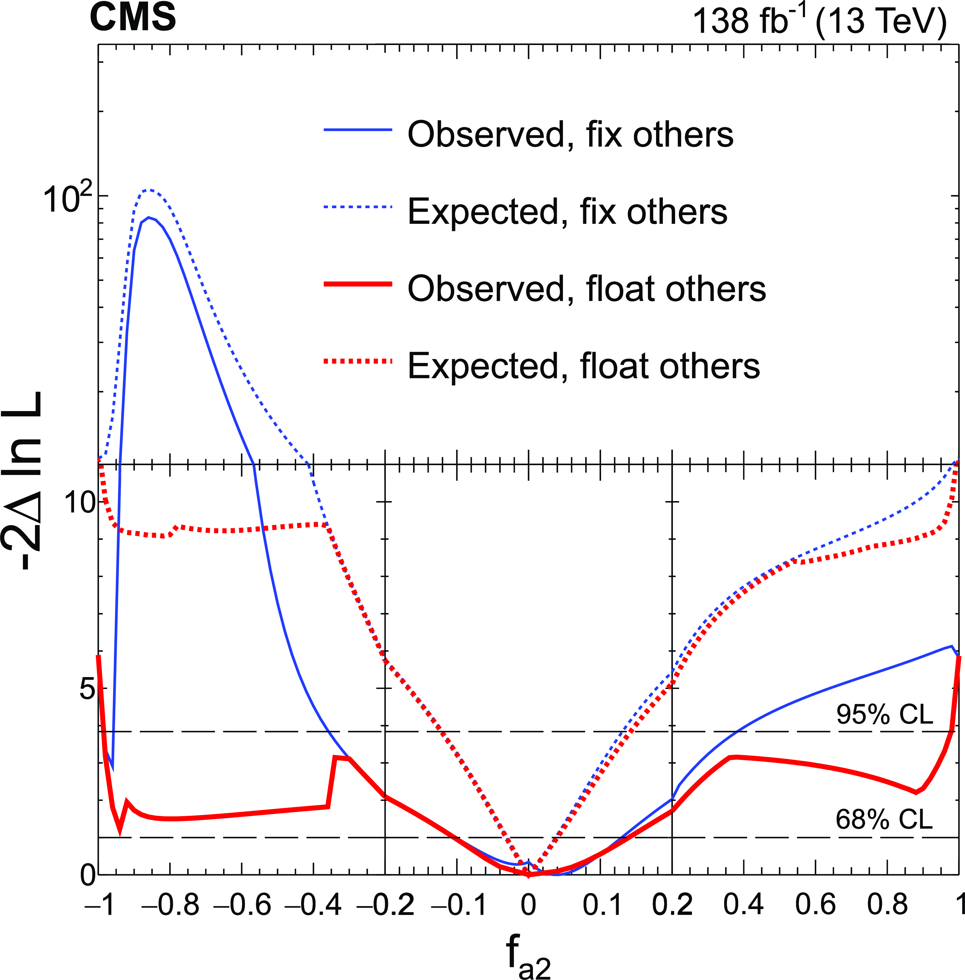
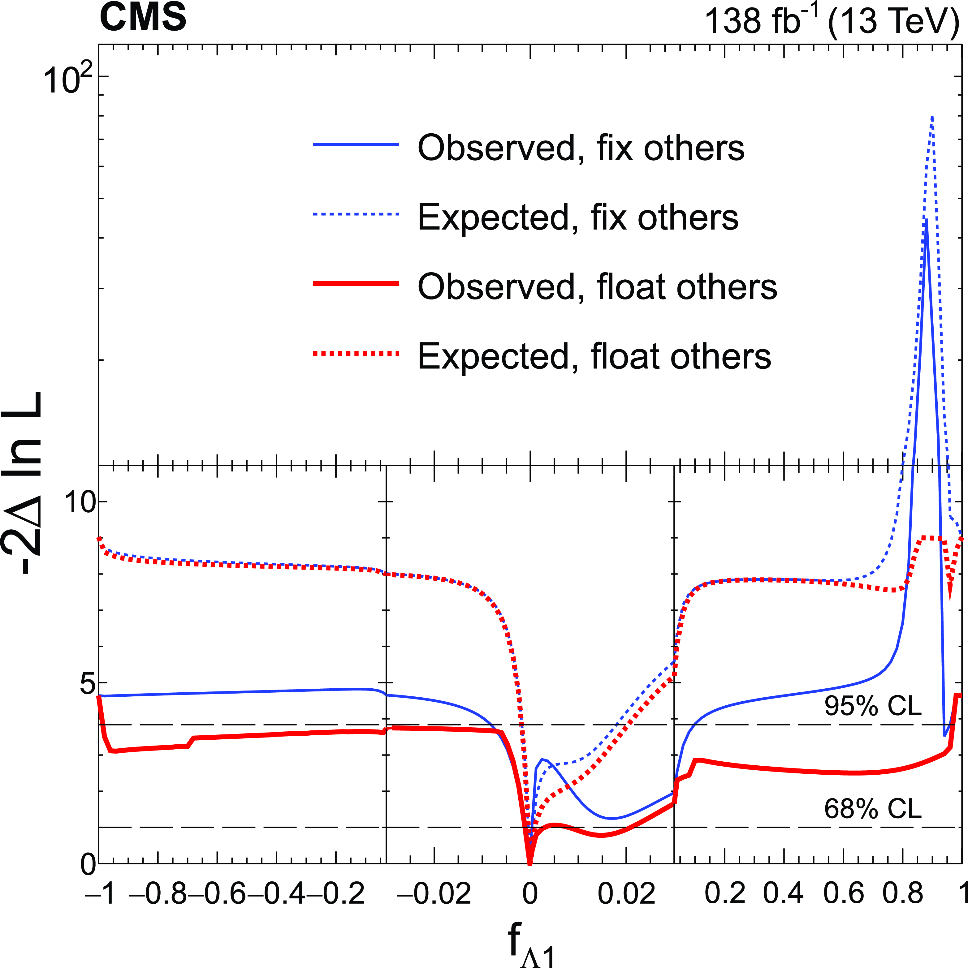
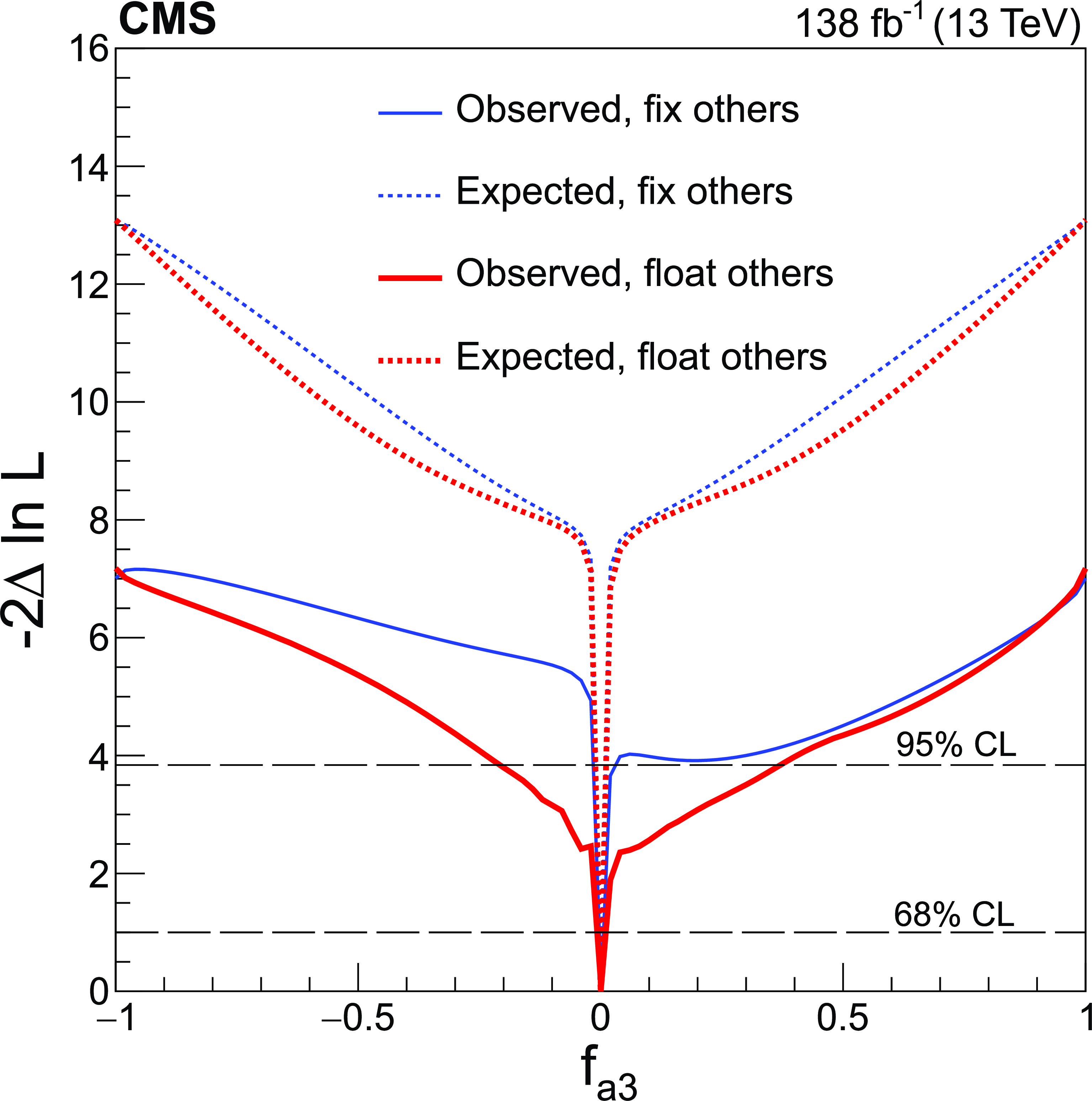
Expected (dashed) and observed (solid) profiled likelihood on $ f_{a2} $ (upper left), $ f_{\Lambda 1} $ (upper right) and $ f_{a3} $ (bottom) using Approach 2. The other two anomalous coupling cross section fractions are either fixed to zero (blue) or left floating in the fit (red). In each case, the signal strength modifiers are treated as free parameters. The dashed horizontal lines show the 68 and 95% CL regions. Axis scales are varied for $ f_{a2} $ and $ f_{\Lambda 1} $ to improve the visibility of important features. |
png pdf |
Figure 9-a:
Expected (dashed) and observed (solid) profiled likelihood on $ f_{a2} $ (upper left), $ f_{\Lambda 1} $ (upper right) and $ f_{a3} $ (bottom) using Approach 2. The other two anomalous coupling cross section fractions are either fixed to zero (blue) or left floating in the fit (red). In each case, the signal strength modifiers are treated as free parameters. The dashed horizontal lines show the 68 and 95% CL regions. Axis scales are varied for $ f_{a2} $ and $ f_{\Lambda 1} $ to improve the visibility of important features. |
png pdf |
Figure 9-b:
Expected (dashed) and observed (solid) profiled likelihood on $ f_{a2} $ (upper left), $ f_{\Lambda 1} $ (upper right) and $ f_{a3} $ (bottom) using Approach 2. The other two anomalous coupling cross section fractions are either fixed to zero (blue) or left floating in the fit (red). In each case, the signal strength modifiers are treated as free parameters. The dashed horizontal lines show the 68 and 95% CL regions. Axis scales are varied for $ f_{a2} $ and $ f_{\Lambda 1} $ to improve the visibility of important features. |
png pdf |
Figure 9-c:
Expected (dashed) and observed (solid) profiled likelihood on $ f_{a2} $ (upper left), $ f_{\Lambda 1} $ (upper right) and $ f_{a3} $ (bottom) using Approach 2. The other two anomalous coupling cross section fractions are either fixed to zero (blue) or left floating in the fit (red). In each case, the signal strength modifiers are treated as free parameters. The dashed horizontal lines show the 68 and 95% CL regions. Axis scales are varied for $ f_{a2} $ and $ f_{\Lambda 1} $ to improve the visibility of important features. |
png pdf |
Figure 10:
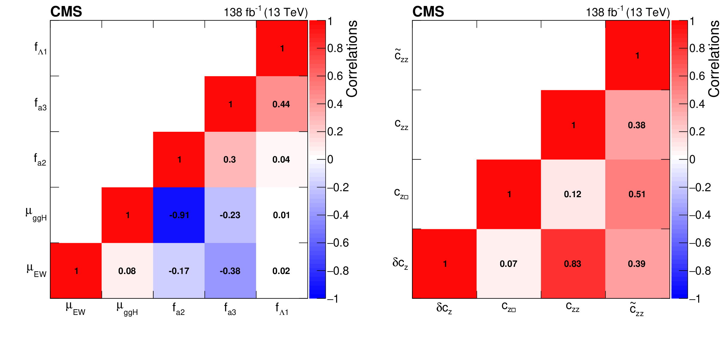
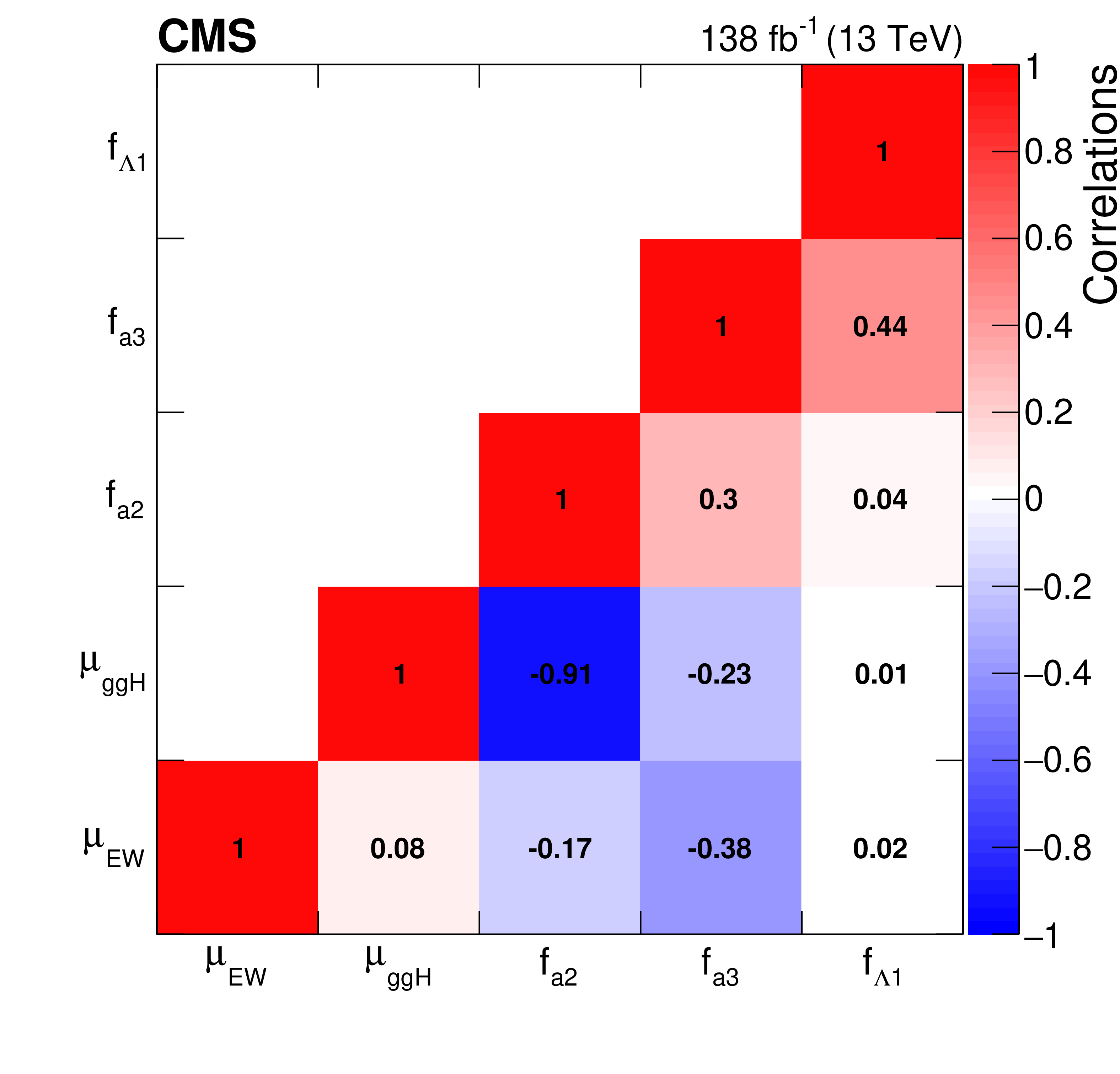
The observed correlation coefficients between HVV anomalous coupling cross section fractions and signal strength modifiers (left) and between SMEFT Higgs basis coupling parameters (right). |
png pdf |
Figure 10-a:
The observed correlation coefficients between HVV anomalous coupling cross section fractions and signal strength modifiers (left) and between SMEFT Higgs basis coupling parameters (right). |

png pdf |
Figure 10-b:
The observed correlation coefficients between HVV anomalous coupling cross section fractions and signal strength modifiers (left) and between SMEFT Higgs basis coupling parameters (right). |
png pdf |
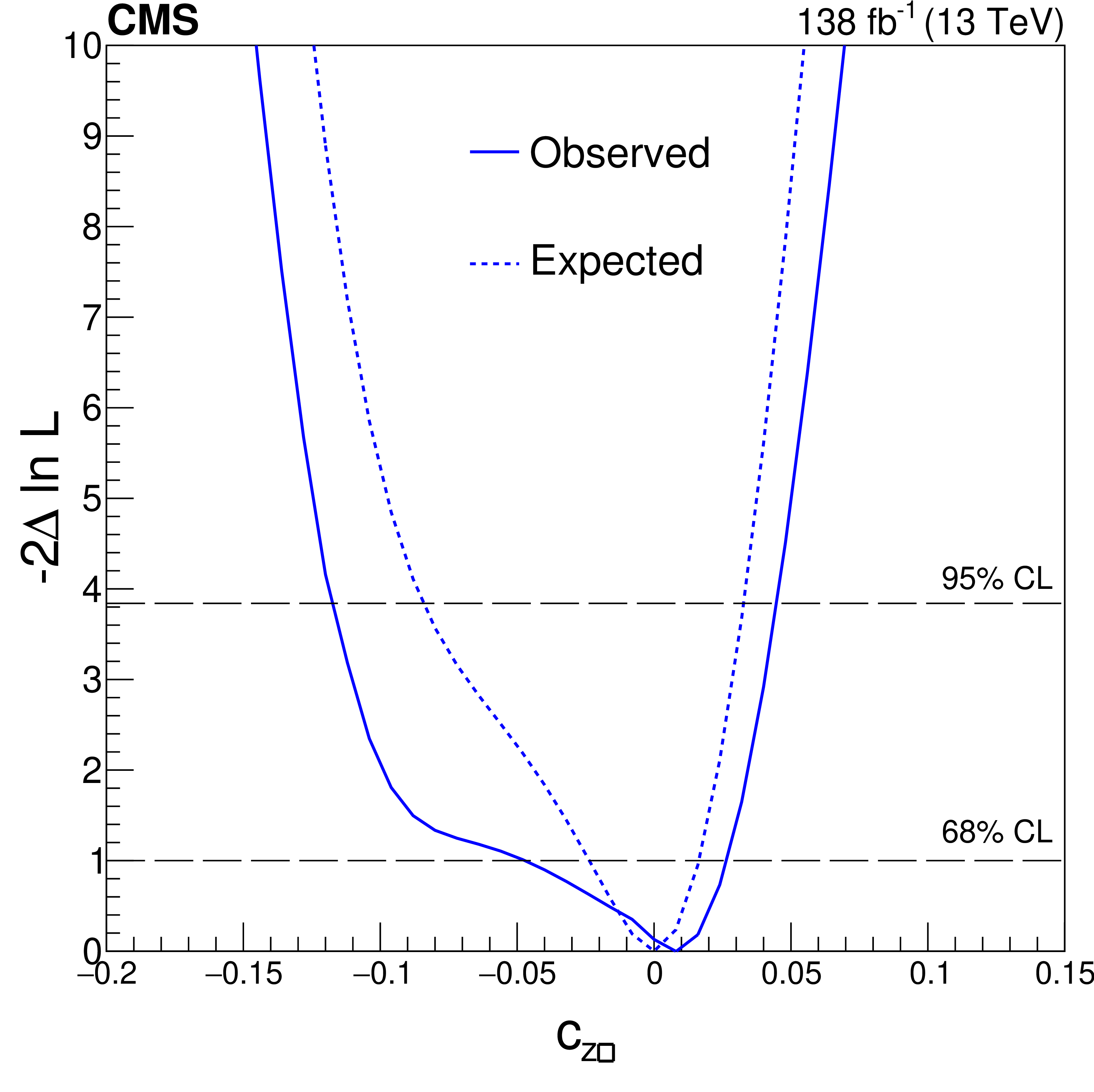
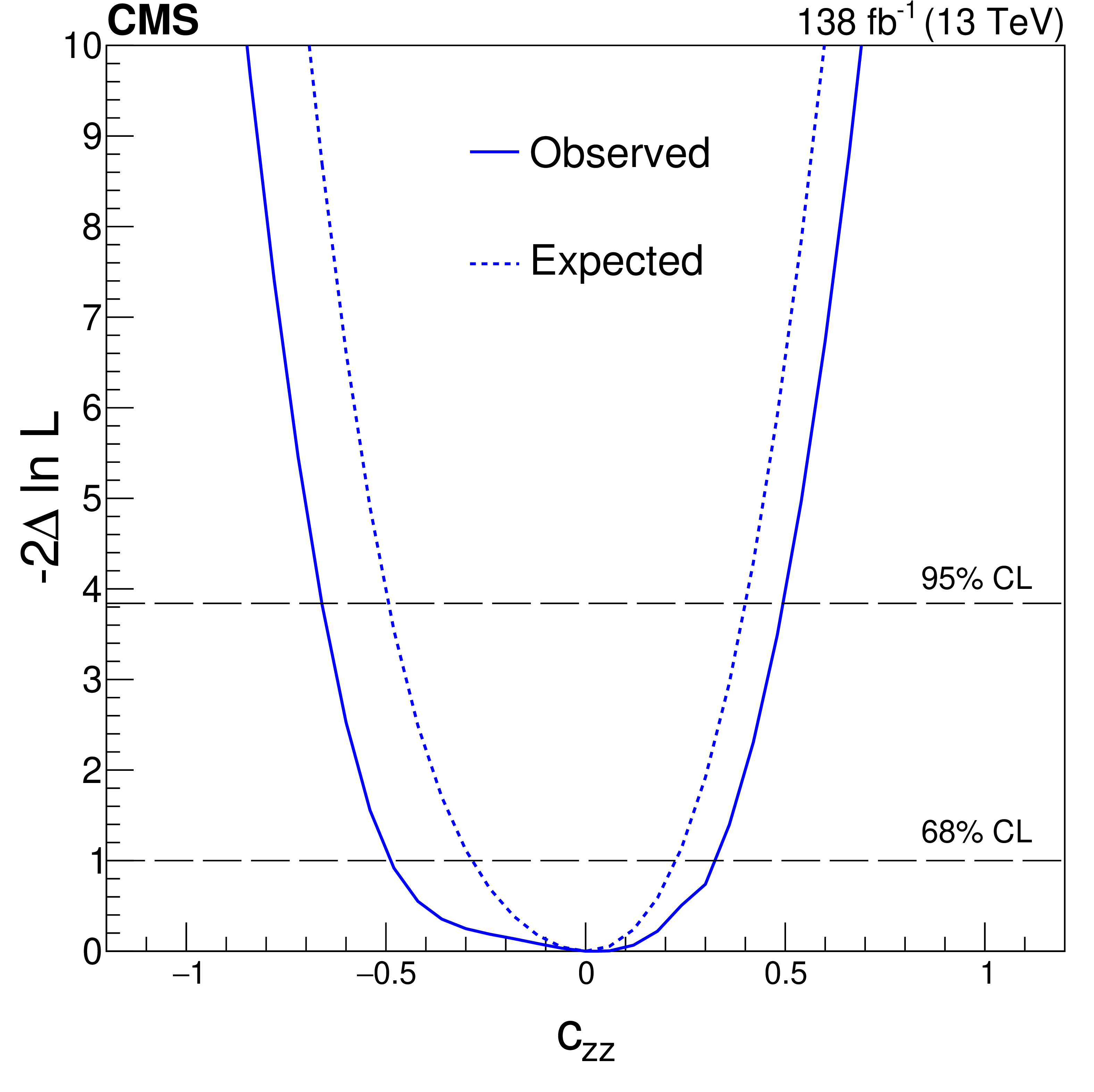
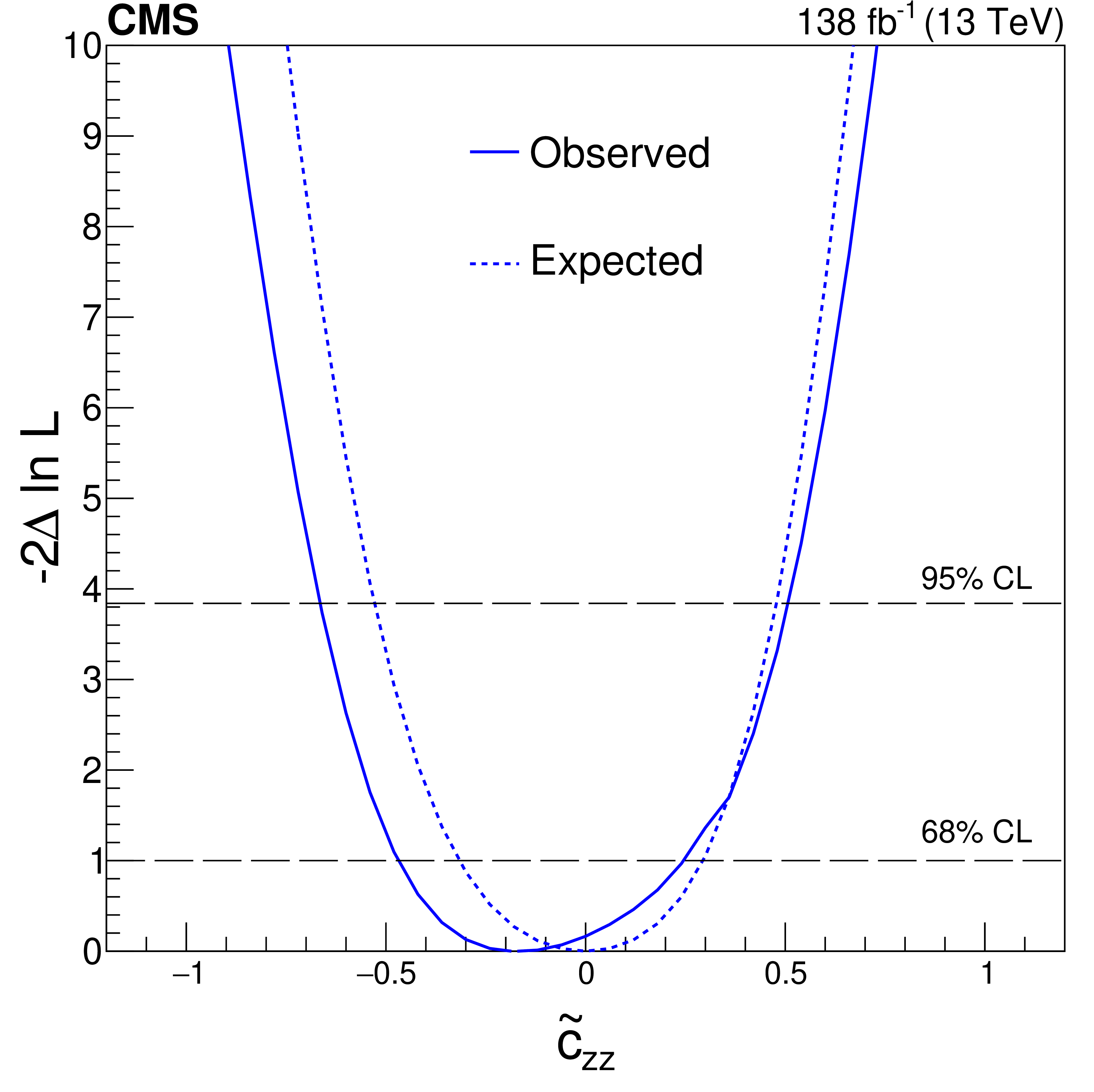
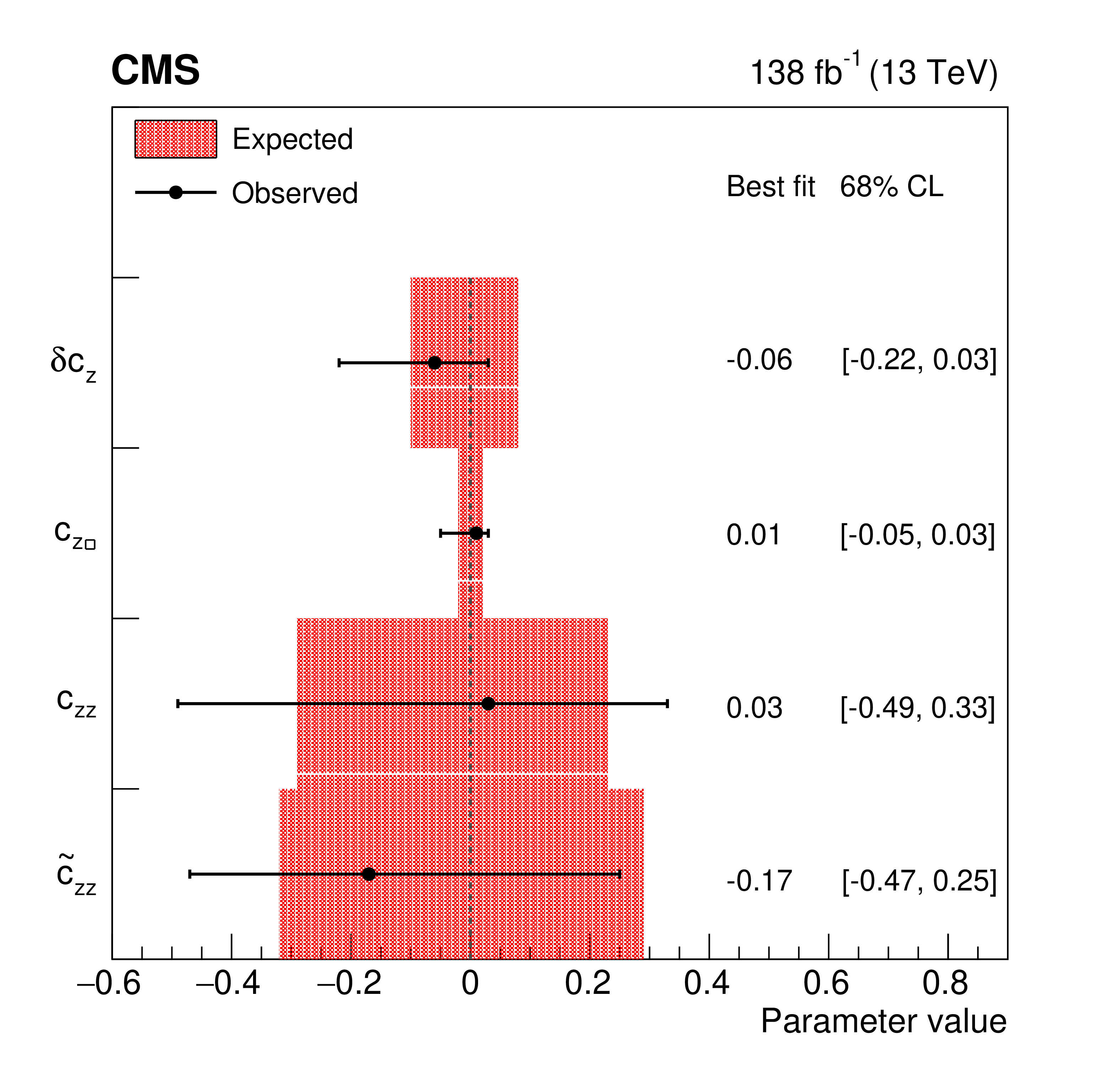
Figure 11:
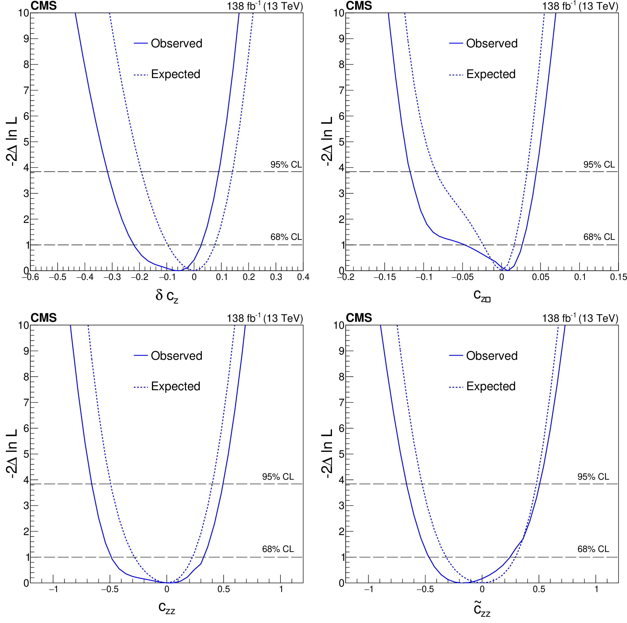
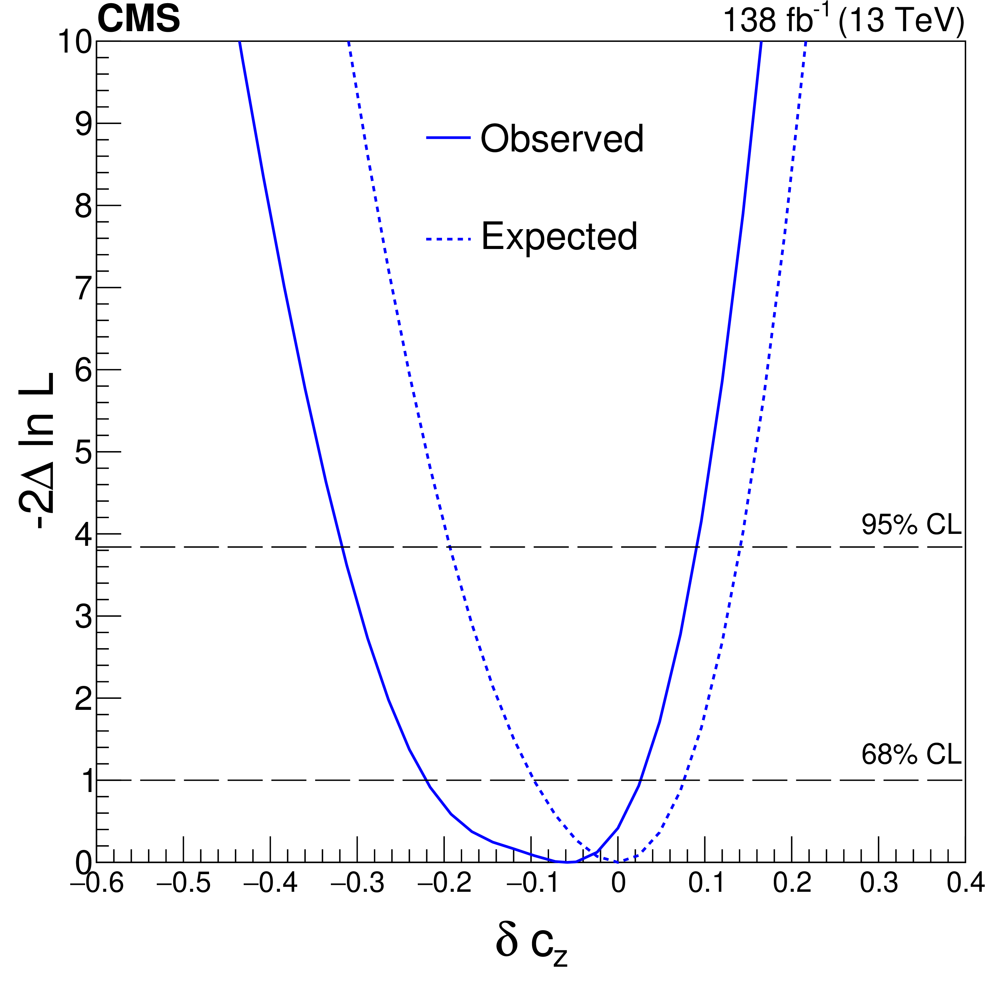
Expected (dashed) and observed (solid) profiled likelihood on the $ \delta c_\text{z} $ (upper left), $ c_{\text{z}\Box} $ (upper right), $ c_\text{zz} $ (lower left), and $ \tilde{c}_\text{zz} $ (lower right) couplings of the SMEFT Higgs basis. All four couplings are studied simultaneously. The dashed horizontal lines show the 68 and 95% CL regions. |
png pdf |
Figure 11-a:
Expected (dashed) and observed (solid) profiled likelihood on the $ \delta c_\text{z} $ (upper left), $ c_{\text{z}\Box} $ (upper right), $ c_\text{zz} $ (lower left), and $ \tilde{c}_\text{zz} $ (lower right) couplings of the SMEFT Higgs basis. All four couplings are studied simultaneously. The dashed horizontal lines show the 68 and 95% CL regions. |
png pdf |
Figure 11-b:
Expected (dashed) and observed (solid) profiled likelihood on the $ \delta c_\text{z} $ (upper left), $ c_{\text{z}\Box} $ (upper right), $ c_\text{zz} $ (lower left), and $ \tilde{c}_\text{zz} $ (lower right) couplings of the SMEFT Higgs basis. All four couplings are studied simultaneously. The dashed horizontal lines show the 68 and 95% CL regions. |
png pdf |
Figure 11-c:
Expected (dashed) and observed (solid) profiled likelihood on the $ \delta c_\text{z} $ (upper left), $ c_{\text{z}\Box} $ (upper right), $ c_\text{zz} $ (lower left), and $ \tilde{c}_\text{zz} $ (lower right) couplings of the SMEFT Higgs basis. All four couplings are studied simultaneously. The dashed horizontal lines show the 68 and 95% CL regions. |
png pdf |
Figure 11-d:
Expected (dashed) and observed (solid) profiled likelihood on the $ \delta c_\text{z} $ (upper left), $ c_{\text{z}\Box} $ (upper right), $ c_\text{zz} $ (lower left), and $ \tilde{c}_\text{zz} $ (lower right) couplings of the SMEFT Higgs basis. All four couplings are studied simultaneously. The dashed horizontal lines show the 68 and 95% CL regions. |
png pdf |
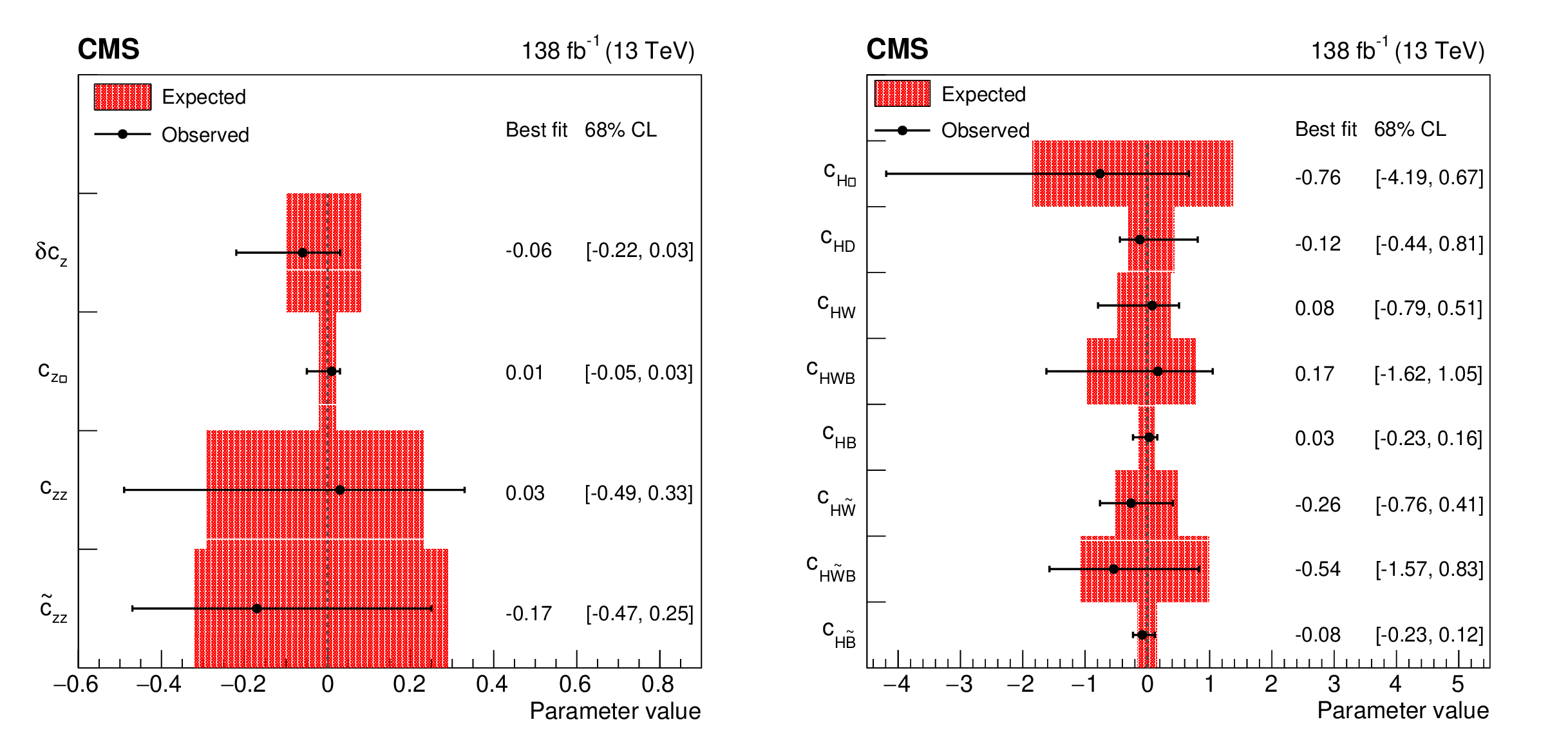
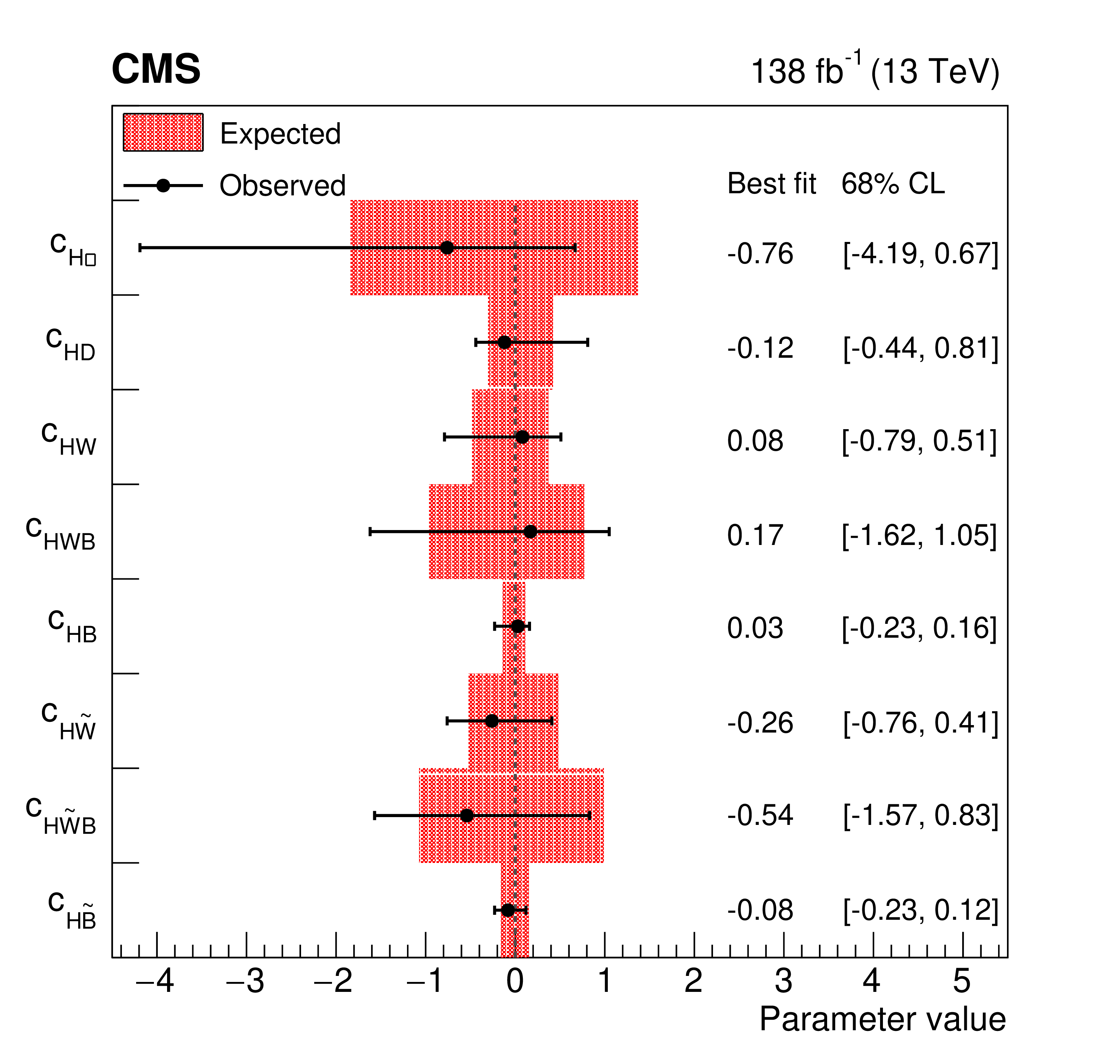
Figure 12:
Summary of constraints on the SMEFT Higgs (left) and Warsaw (right) basis coupling parameters with the best fit values and 68% CL uncertainties. For the Warsaw basis, only one of $ c_\text{HW} $, $ c_\text{HWB} $, and $ c_\text{HB} $ is independent, the same is also true for $ c_{\text{H}\tilde{\text{W}}} $, $ c_{\text{H}\tilde{\text{W}}\text{B}} $, and $ c_{\text{H}\tilde{\text{B}}} $. |
png pdf |
Figure 12-a:
Summary of constraints on the SMEFT Higgs (left) and Warsaw (right) basis coupling parameters with the best fit values and 68% CL uncertainties. For the Warsaw basis, only one of $ c_\text{HW} $, $ c_\text{HWB} $, and $ c_\text{HB} $ is independent, the same is also true for $ c_{\text{H}\tilde{\text{W}}} $, $ c_{\text{H}\tilde{\text{W}}\text{B}} $, and $ c_{\text{H}\tilde{\text{B}}} $. |
png pdf |
Figure 12-b:
Summary of constraints on the SMEFT Higgs (left) and Warsaw (right) basis coupling parameters with the best fit values and 68% CL uncertainties. For the Warsaw basis, only one of $ c_\text{HW} $, $ c_\text{HWB} $, and $ c_\text{HB} $ is independent, the same is also true for $ c_{\text{H}\tilde{\text{W}}} $, $ c_{\text{H}\tilde{\text{W}}\text{B}} $, and $ c_{\text{H}\tilde{\text{B}}} $. |
png pdf |
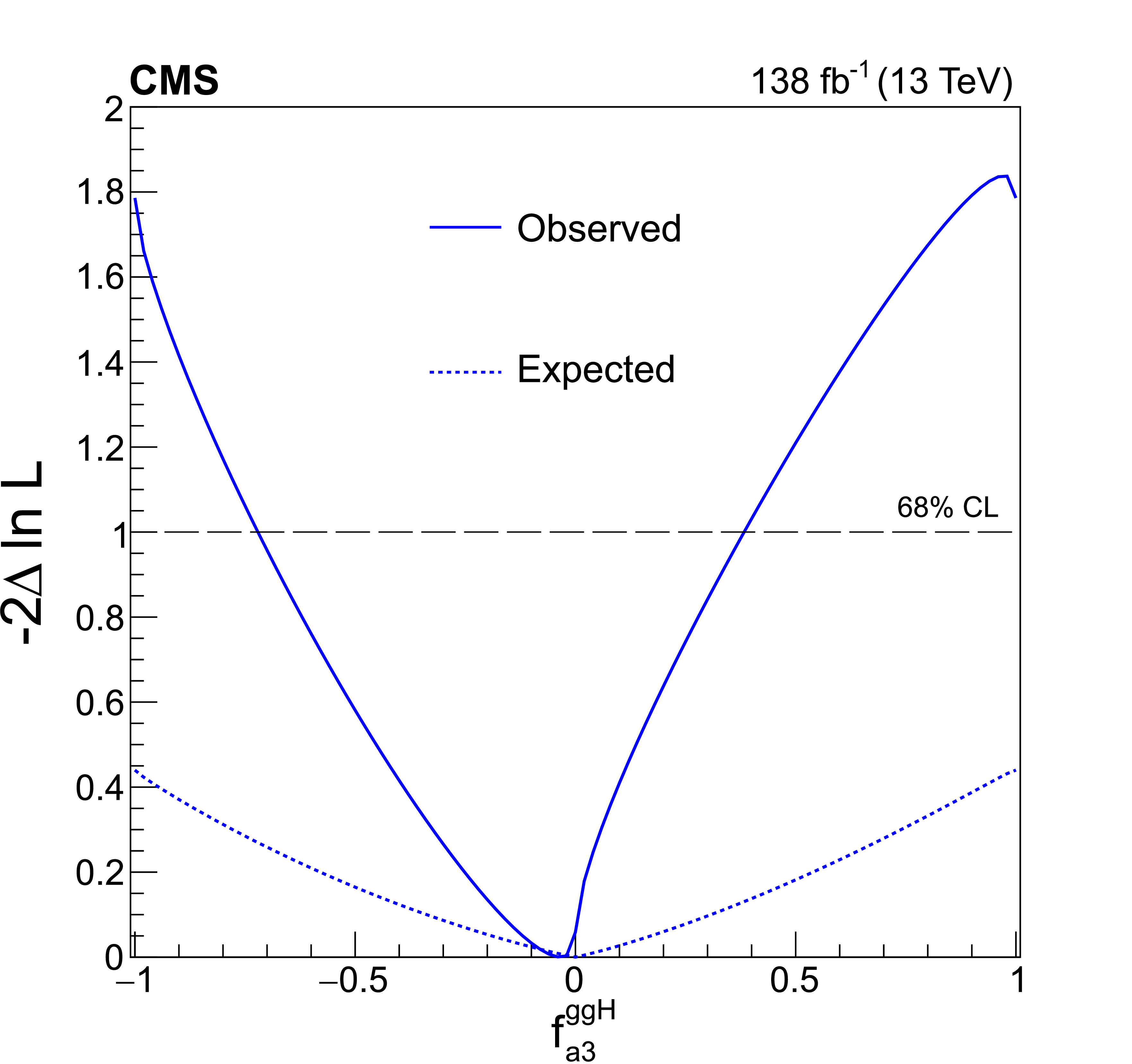
Figure 13:
Expected (dashed) and observed (solid) profiled likelihood on $ f_{a3}^{\mathrm{g}\mathrm{g}\mathrm{H}} $. The signal strength modifiers and the CP-odd HVV anomalous coupling cross section fraction are treated as free parameters. The crossing of the observed likelihood with the dashed horizontal line shows the observed 68% CL region. |
| Tables | |
png pdf |
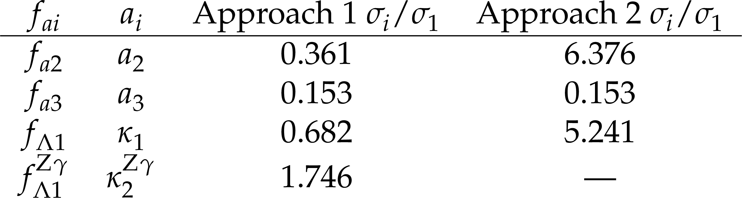
Table 1:
The cross sections ($ \sigma_i $) of the anomalous contributions ($ a_i $) relative to the SM value ($ \sigma_1 $) used to define the fractional cross sections $ f_{ai} $ for the Approach 1 and 2 coupling relationships. For the $ \kappa_{1} $ and $ \kappa_{2}^{\mathrm{Z}\gamma} $ couplings, the numerical values $ \Lambda_1 = \Lambda_1^{\mathrm{Z}\gamma} = $ 100 GeV are chosen to keep all coefficients of similar order of magnitude. |
png pdf |
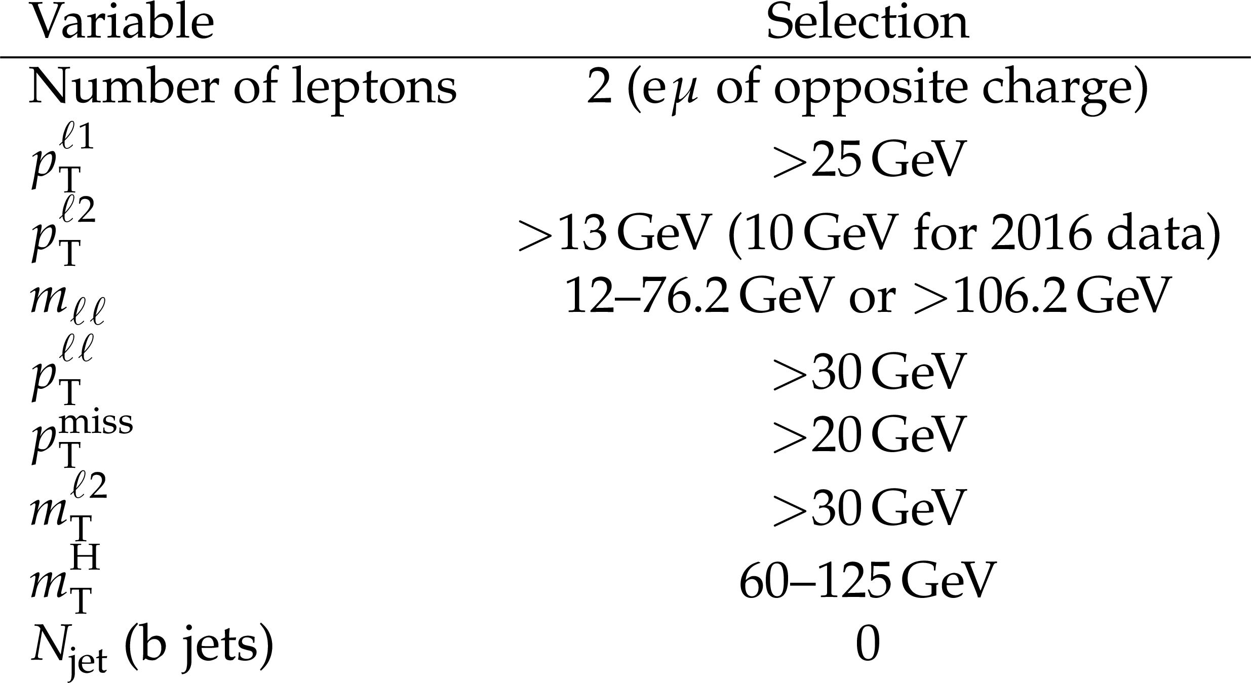
Table 2:
Summary of the base selection criteria. |
png pdf |
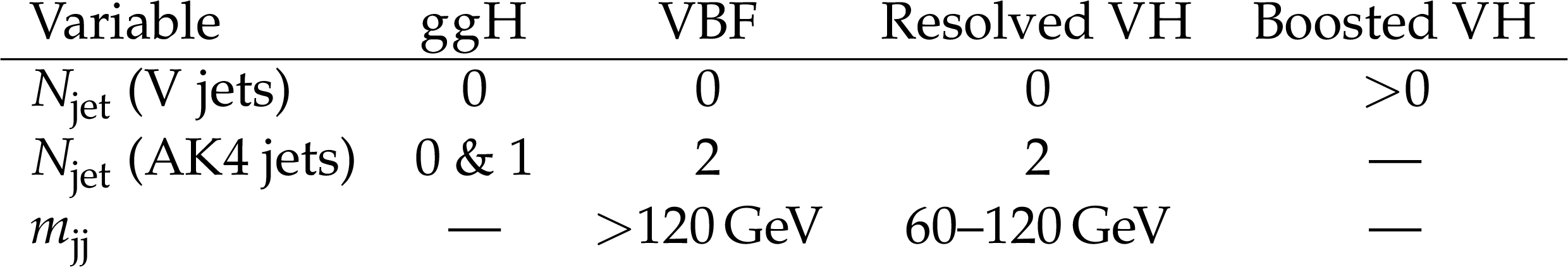
Table 3:
Summary of the ggH, VBF, and VH production channels used for the HVV coupling study. |
png pdf |
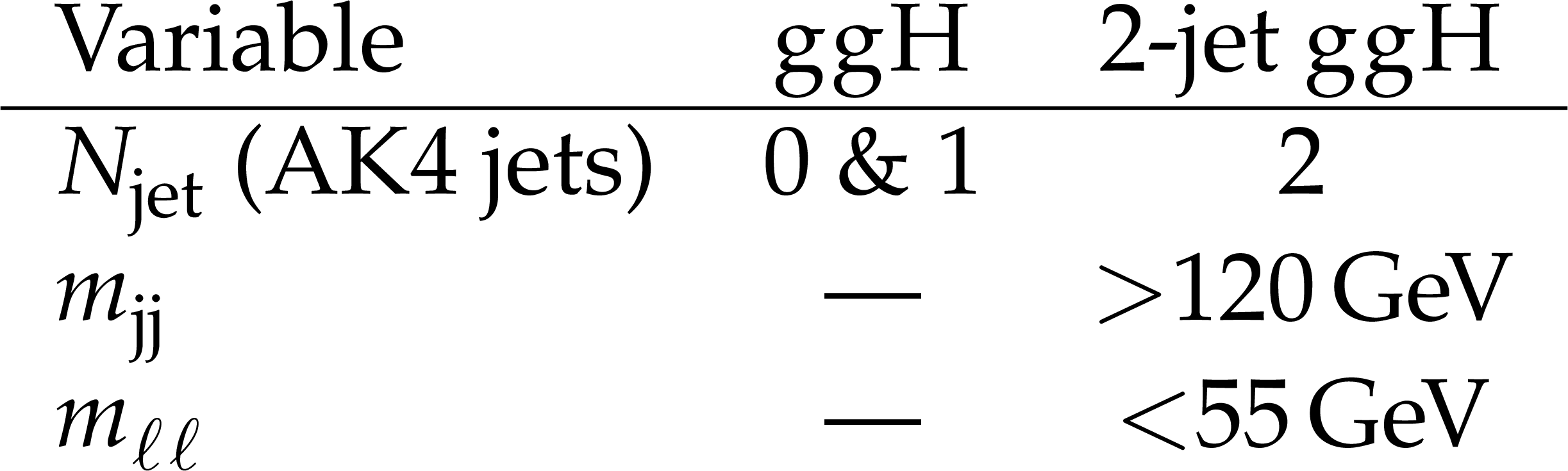
Table 4:
Summary of ggH channel selections used for the Hgg coupling study. |
png pdf |
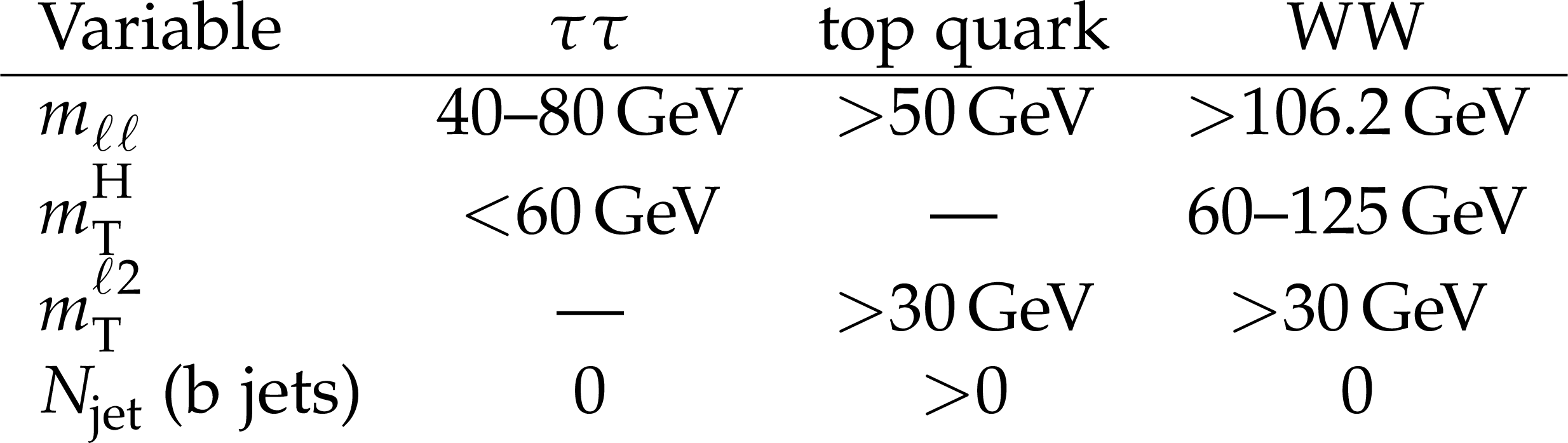
Table 5:
Summary of the $ \tau\tau $, top quark, and WW control region requirements. |

png pdf |
Table 6:
The kinematic observables used for the interference based categorization and for the final discriminants used in the fits to data to study the HVV and Hgg couplings. For each of the anomalous HVV couplings in Approach 1, we have a dedicated analysis in the VBF and VH channels. In Approach 2, we use one analysis to target all anomalous HVV couplings simultaneously. |

png pdf |
Table 7:
Summary of constraints on the anomalous HVV and Hgg coupling parameters with the best fit values and allowed 68 and 95% CL (in square brackets) intervals. For Approach 1, each $ f_{ai} $ is studied independently. For Approach 2, each $ f_{ai} $ is shown separately with the other two cross section fractions either fixed to zero or left floating in the fit. In each case, the signal strength modifiers are treated as free parameters. |
png pdf |
Table 8:
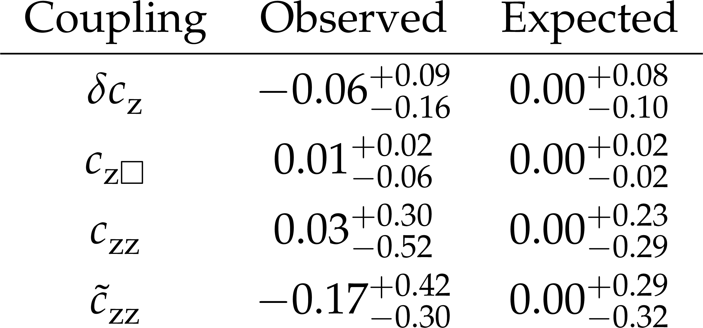
Summary of constraints on the SMEFT Higgs basis coupling parameters with the best fit values and 68% CL uncertainties. All four couplings are studied simultaneously. |
png pdf |
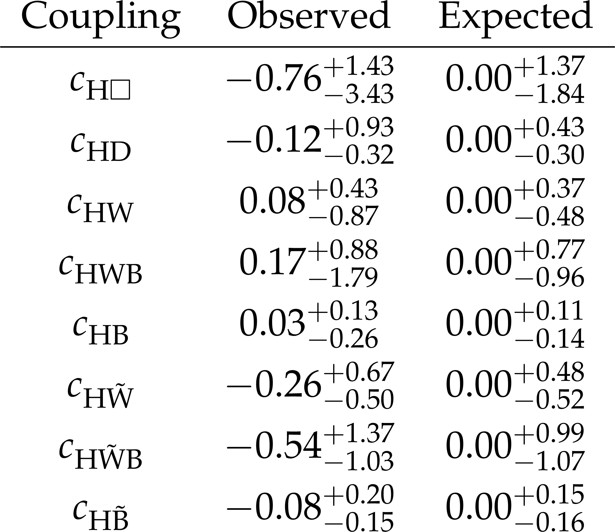
Table 9:
Summary of constraints on the SMEFT Warsaw basis coupling parameters with the best fit values and 68% CL uncertainties. Only one of $ c_\text{HW} $, $ c_\text{HWB} $, and $ c_\text{HB} $ is independent, the same is also true for $ c_{\text{H}\tilde{\text{W}}} $, $ c_{\text{H}\tilde{\text{W}}\text{B}} $, and $ c_{\text{H}\tilde{\text{B}}} $. Three independent fits to the data were performed with a different choice of four independent couplings in each. |
| Summary |
| This paper presents a study of the anomalous couplings of the Higgs boson (H) with vector bosons, including CP violating effects, using its associated production with hadronic jets in gluon fusion, electroweak vector boson fusion, and associated production with a W or Z boson, and its subsequent decay to a pair of W bosons. The results are based on the proton-proton collision data set collected by the CMS detector at the LHC during 2016-2018, corresponding to an integrated luminosity of 138 fb$ ^{-1} $ at a center-of-mass energy of 13 TeV. The analysis targets the different-flavor dilepton ($ \mathrm{e}\mu $) final state, with kinematic information from associated jets combined using matrix element techniques to increase sensitivity to anomalous effects at the production vertex. Dedicated Monte Carlo simulation and matrix element reweighting provide modeling of all kinematic features in the production and decay of the Higgs boson with full simulation of detector effects. A simultaneous measurement of four Higgs boson couplings to electroweak vector bosons has been performed in the framework of a standard model effective field theory. All measurements are consistent with the expectations for the standard model Higgs boson and constraints are set on the fractional contribution of the anomalous couplings to the Higgs boson cross section. The most stringent constraints on the HVV anomalous coupling cross section fractions are at the per mille level. These results are in agreement with those obtained in the $ \mathrm{H}\to\mathrm{Z}\mathrm{Z} $ and $ \mathrm{H}\to\tau\tau $ channels, and also significantly surpass those of the previous $ \mathrm{H}\to\mathrm{W}\mathrm{W} $ anomalous coupling analysis from the CMS experiment in both scope and precision. |
| References | ||||
| 1 | ATLAS Collaboration | Observation of a new particle in the search for the standard model Higgs boson with the ATLAS detector at the LHC | PLB 716 (2012) 1 | 1207.7214 |
| 2 | CMS Collaboration | Observation of a new boson at a mass of 125 GeV with the CMS experiment at the LHC | PLB 716 (2012) 30 | CMS-HIG-12-028 1207.7235 |
| 3 | CMS Collaboration | Observation of a new boson with mass near 125 GeV in pp collisions at $ \sqrt{s}= $ 7 and 8 TeV | JHEP 06 (2013) 081 | CMS-HIG-12-036 1303.4571 |
| 4 | CMS Collaboration | On the mass and spin-parity of the Higgs boson candidate via its decays to Z boson pairs | PRL 110 (2013) 081803 | CMS-HIG-12-041 1212.6639 |
| 5 | CMS Collaboration | Measurement of the properties of a Higgs boson in the four-lepton final state | PRD 89 (2014) 092007 | CMS-HIG-13-002 1312.5353 |
| 6 | CMS Collaboration | Constraints on the spin-parity and anomalous HVV couplings of the Higgs boson in proton collisions at 7 and 8 TeV | PRD 92 (2015) 012004 | CMS-HIG-14-018 1411.3441 |
| 7 | CMS Collaboration | Limits on the Higgs boson lifetime and width from its decay to four charged leptons | PRD 92 (2015) 072010 | CMS-HIG-14-036 1507.06656 |
| 8 | CMS Collaboration | Combined search for anomalous pseudoscalar HVV couplings in VH production and $ \mathrm{H}\to \mathrm{V}\mathrm{V} $ decay | PLB 759 (2016) 672 | CMS-HIG-14-035 1602.04305 |
| 9 | CMS Collaboration | Constraints on anomalous Higgs boson couplings using production and decay information in the four-lepton final state | PLB 775 (2017) 1 | CMS-HIG-17-011 1707.00541 |
| 10 | CMS Collaboration | Measurements of the Higgs boson width and anomalous HVV couplings from on-shell and off-shell production in the four-lepton final state | PRD 99 (2019) 112003 | CMS-HIG-18-002 1901.00174 |
| 11 | CMS Collaboration | Constraints on anomalous $ \mathrm{H}\mathrm{V}\mathrm{V} $ couplings from the production of Higgs bosons decaying to $ \tau $ lepton pairs | PRD 100 (2019) 112002 | CMS-HIG-17-034 1903.06973 |
| 12 | ATLAS Collaboration | Evidence for the spin-0 nature of the Higgs boson using ATLAS data | PLB 726 (2013) 120 | 1307.1432 |
| 13 | ATLAS Collaboration | Study of the spin and parity of the Higgs boson in diboson decays with the ATLAS detector | EPJC 75 (2015) 476 | 1506.05669 |
| 14 | ATLAS Collaboration | Test of $ CP $ invariance in vector-boson fusion production of the Higgs boson using the Optimal Observable method in the ditau decay channel with the ATLAS detector | EPJC 76 (2016) 658 | 1602.04516 |
| 15 | ATLAS Collaboration | Measurement of inclusive and differential cross sections in the $ \mathrm{H} \rightarrow \mathrm{Z}\mathrm{Z}^{*} \rightarrow 4\ell $ decay channel in pp collisions at $ \sqrt{s}= $ 13 TeV with the ATLAS detector | JHEP 10 (2017) 132 | 1708.02810 |
| 16 | ATLAS Collaboration | Measurement of the Higgs boson coupling properties in the $ \mathrm{H} \rightarrow \mathrm{Z}\mathrm{Z}^{*} \rightarrow 4\ell $ decay channel at $ \sqrt{s} $ = 13 TeV with the ATLAS detector | JHEP 03 (2018) 095 | 1712.02304 |
| 17 | ATLAS Collaboration | Measurements of Higgs boson properties in the diphoton decay channel with 36 fb$ ^{-1} $ of pp collision data at $ \sqrt{s} = $ 13 TeV with the ATLAS detector | PRD 98 (2018) 052005 | 1802.04146 |
| 18 | ATLAS Collaboration | Test of $ CP $ invariance in vector-boson fusion production of the Higgs boson in the $ \mathrm {H}\rightarrow\tau\tau $ channel in proton-proton collisions at $ \sqrt{s} $ = 13 TeV with the ATLAS detector | PLB 805 (2020) 135426 | 2002.05315 |
| 19 | LHC Higgs Cross Section Working Group | Handbook of LHC Higgs cross sections: 4. Deciphering the nature of the Higgs sector | CERN Report CERN-2017-002-M, 2016 link |
1610.07922 |
| 20 | Y. Gao et al. | Spin determination of single-produced resonances at hadron colliders | PRD 81 (2010) 075022 | 1001.3396 |
| 21 | S. Bolognesi et al. | On the spin and parity of a single-produced resonance at the LHC | PRD 86 (2012) 095031 | 1208.4018 |
| 22 | I. Anderson et al. | Constraining anomalous HVV interactions at proton and lepton colliders | PRD 89 (2014) 035007 | 1309.4819 |
| 23 | A. V. Gritsan, R. Röntsch, M. Schulze, and M. Xiao | Constraining anomalous Higgs boson couplings to the heavy flavor fermions using matrix element techniques | PRD 94 (2016) 055023 | 1606.03107 |
| 24 | A. V. Gritsan et al. | New features in the JHU generator framework: constraining Higgs boson properties from on-shell and off-shell production | PRD 102 (2020) 056022 | 2002.09888 |
| 25 | CMS Collaboration | Measurements of the Higgs boson production cross section and couplings in the W boson pair decay channel in proton-proton collisions at $ \sqrt{s} $ = 13 TeV | EPJC 83 (2023) 667 | CMS-HIG-20-013 2206.09466 |
| 26 | LHC Higgs Cross Section Working Group | Handbook of LHC Higgs cross sections: 3. Higgs Properties: Report of the LHC Higgs Cross Section Working Group | CERN Report CERN-2013-004, 2013 link |
1307.1347 |
| 27 | CMS Collaboration | Measurements of $ {\mathrm{t}\overline{\mathrm{t}}} \mathrm{H} $ production and the $ CP $ structure of the Yukawa interaction between the Higgs boson and top quark in the diphoton decay channel | PRL 125 (2020) 061801 | CMS-HIG-19-013 2003.10866 |
| 28 | CMS Collaboration | Constraints on anomalous Higgs boson couplings to vector bosons and fermions in its production and decay using the four-lepton final state | PRD 104 (2021) 052004 | CMS-HIG-19-009 2104.12152 |
| 29 | CMS Collaboration | HEPData record for this analysis | link | |
| 30 | B. Grzadkowski, M. Iskrzy \' n ski, M. Misiak, and J. Rosiek | Dimension-six terms in the standard model lagrangian | JHEP 10 (2010) 085 | 1008.4884 |
| 31 | J. Davis et al. | Constraining anomalous Higgs boson couplings to virtual photons | PRD 105 (2022) 096027 | 2109.13363 |
| 32 | A. V. Gritsan et al. | New features in the JHU generator framework: Constraining Higgs boson properties from on-shell and off-shell production | PRD 102 (2020) | |
| 33 | CMS Collaboration | The CMS experiment at the CERN LHC | JINST 3 (2008) S08004 | |
| 34 | CMS Collaboration | Performance of electron reconstruction and selection with the CMS detector in proton-proton collisions at $ \sqrt{s} = $ 8 TeV | JINST 10 (2015) P06005 | CMS-EGM-13-001 1502.02701 |
| 35 | CMS Collaboration | Performance of the CMS muon detector and muon reconstruction with proton-proton collisions at $ \sqrt{s}= $ 13 TeV | JINST 13 (2018) P06015 | CMS-MUO-16-001 1804.04528 |
| 36 | CMS Collaboration | Performance of photon reconstruction and identification with the CMS detector in proton-proton collisions at sqrt(s) = 8 TeV | JINST 10 (2015) P08010 | CMS-EGM-14-001 1502.02702 |
| 37 | CMS Collaboration | Description and performance of track and primary-vertex reconstruction with the CMS tracker | JINST 9 (2014) P10009 | CMS-TRK-11-001 1405.6569 |
| 38 | CMS Collaboration | Particle-flow reconstruction and global event description with the CMS detector | JINST 12 (2017) P10003 | CMS-PRF-14-001 1706.04965 |
| 39 | CMS Collaboration | Performance of reconstruction and identification of $ \tau $ leptons decaying to hadrons and $ \nu_\tau $ in pp collisions at $ \sqrt{s}= $ 13 TeV | JINST 13 (2018) P10005 | CMS-TAU-16-003 1809.02816 |
| 40 | CMS Collaboration | Jet energy scale and resolution in the CMS experiment in pp collisions at 8 TeV | JINST 12 (2017) P02014 | CMS-JME-13-004 1607.03663 |
| 41 | CMS Collaboration | Performance of missing transverse momentum reconstruction in proton-proton collisions at $ \sqrt{s} = $ 13\,TeV using the CMS detector | JINST 14 (2019) P07004 | CMS-JME-17-001 1903.06078 |
| 42 | CMS Collaboration | Performance of the CMS Level-1 trigger in proton-proton collisions at $ \sqrt{s} = $ 13\,TeV | JINST 15 (2020) P10017 | CMS-TRG-17-001 2006.10165 |
| 43 | CMS Collaboration | The CMS trigger system | JINST 12 (2017) P01020 | CMS-TRG-12-001 1609.02366 |
| 44 | CMS Collaboration | Precision luminosity measurement in proton-proton collisions at $ \sqrt{s}= $ 13 TeV in 2015 and 2016 at CMS | EPJC 800 (2021) 81 | CMS-LUM-17-003 2104.01927 |
| 45 | CMS Collaboration | CMS luminosity measurement for the 2017 data-taking period at $ \sqrt{s} = $ 13 TeV | CMS Physics Analysis Summary, 2017 CMS-PAS-LUM-17-004 |
CMS-PAS-LUM-17-004 |
| 46 | CMS Collaboration | CMS luminosity measurement for the 2018 data-taking period at $ \sqrt{s} = $ 13 TeV | CMS Physics Analysis Summary, 2019 CMS-PAS-LUM-18-002 |
CMS-PAS-LUM-18-002 |
| 47 | NNPDF Collaboration | Parton distributions with QED corrections | NPB 877 (2013) 290 | 1308.0598 |
| 48 | NNPDF Collaboration | Unbiased global determination of parton distributions and their uncertainties at NNLO and at LO | NPB 855 (2012) 153 | 1107.2652 |
| 49 | NNPDF Collaboration | Parton distributions from high-precision collider data | EPJC 77 (2017) 663 | 1706.00428 |
| 50 | CMS Collaboration | Event generator tunes obtained from underlying event and multiparton scattering measurements | EPJC 76 (2016) 155 | CMS-GEN-14-001 1512.00815 |
| 51 | CMS Collaboration | Extraction and validation of a new set of CMS \textscPYTHIA8 tunes from underlying-event measurements | EPJC 80 (2020) 4 | CMS-GEN-17-001 1903.12179 |
| 52 | T. Sjöstrand et al. | An introduction to PYTHIA 8.2 | Comput. Phys. Commun. 191 (2015) 159 | 1410.3012 |
| 53 | P. Nason | A new method for combining NLO QCD with shower Monte Carlo algorithms | JHEP 11 (2004) 040 | hep-ph/0409146 |
| 54 | S. Frixione, P. Nason, and C. Oleari | Matching NLO QCD computations with parton shower simulations: the POWHEG method | JHEP 11 (2007) 070 | 0709.2092 |
| 55 | S. Alioli, P. Nason, C. Oleari, and E. Re | A general framework for implementing NLO calculations in shower Monte Carlo programs: the POWHEG BOX | JHEP 06 (2010) 043 | 1002.2581 |
| 56 | E. Bagnaschi, G. Degrassi, P. Slavich, and A. Vicini | Higgs production via gluon fusion in the POWHEG approach in the SM and in the MSSM | JHEP 02 (2012) 088 | 1111.2854 |
| 57 | P. Nason and C. Oleari | NLO Higgs boson production via vector-boson fusion matched with shower in POWHEG | JHEP 02 (2010) 037 | 0911.5299 |
| 58 | G. Luisoni, P. Nason, C. Oleari, and F. Tramontano | $ \mathrm{HW^{\pm}} $/HZ + 0 and 1 jet at NLO with the POWHEG BOX interfaced to GoSam and their merging within MiNLO | JHEP 10 (2013) 083 | 1306.2542 |
| 59 | H. B. Hartanto, B. Jager, L. Reina, and D. Wackeroth | Higgs boson production in association with top quarks in the POWHEG BOX | PRD 91 (2015) 094003 | 1501.04498 |
| 60 | K. Hamilton, P. Nason, E. Re, and G. Zanderighi | NNLOPS simulation of Higgs boson production | JHEP 10 (2013) 222 | 1309.0017 |
| 61 | K. Hamilton, P. Nason, and G. Zanderighi | Finite quark-mass effects in the NNLOPS POWHEG+MiNLO Higgs generator | JHEP 05 (2015) 140 | 1501.04637 |
| 62 | N. Berger et al. | Simplified template cross sections --- stage 1.1 | 1906.02754 | |
| 63 | R. Frederix and K. Hamilton | Extending the MINLO method | JHEP 05 (2016) 042 | 1512.02663 |
| 64 | J. Alwall et al. | The automated computation of tree-level and next-to-leading order differential cross sections, and their matching to parton shower simulations | JHEP 07 (2014) 079 | 1405.0301 |
| 65 | CMS Collaboration | A measurement of the Higgs boson mass in the diphoton decay channel | PLB 805 (2020) 135425 | CMS-HIG-19-004 2002.06398 |
| 66 | P. Nason, C. Oleari, M. Rocco, and M. Zaro | An interface between the POWHEG BOX and MadGraph5\_aMC@NLO | EPJC 80 (2020) 10 | 2008.06364 |
| 67 | P. Nason and G. Zanderighi | $ W^+ W^- $, $ W Z $ and $ Z Z $ production in the POWHEG-BOX-V2 | EPJC 74 (2014) 2702 | 1311.1365 |
| 68 | P. Meade, H. Ramani, and M. Zeng | Transverse momentum resummation effects in $ \mathrm{W}^+\mathrm{W}^- $ measurements | PRD 90 (2014) 114006 | 1407.4481 |
| 69 | P. Jaiswal and T. Okui | Explanation of the $ \mathrm{W}\mathrm{W} $ excess at the LHC by jet-veto resummation | PRD 90 (2014) 073009 | 1407.4537 |
| 70 | J. M. Campbell and R. K. Ellis | An update on vector boson pair production at hadron colliders | PRD 60 (1999) 113006 | hep-ph/9905386 |
| 71 | J. M. Campbell, R. K. Ellis, and C. Williams | Vector boson pair production at the LHC | JHEP 07 (2011) 018 | 1105.0020 |
| 72 | J. M. Campbell, R. K. Ellis, and W. T. Giele | A multi-threaded version of MCFM | EPJC 75 (2015) 246 | 1503.06182 |
| 73 | F. Caola et al. | QCD corrections to vector boson pair production in gluon fusion including interference effects with off-shell Higgs at the LHC | JHEP 07 (2016) 087 | 1605.04610 |
| 74 | Alwall, J. and others | Comparative study of various algorithms for the merging of parton showers and matrix elements in hadronic collisions | EPJC 53 (2008) 473 | 0706.2569 |
| 75 | S. Frixione, P. Nason, and G. Ridolfi | A positive-weight next-to-leading-order Monte Carlo for heavy flavour hadroproduction | JHEP 09 (2007) 126 | 0707.3088 |
| 76 | S. Alioli, P. Nason, C. Oleari, and E. Re | NLO single-top production matched with shower in POWHEG: $ s $- and $ t $-channel contributions | JHEP 09 (2009) 111 | 0907.4076 |
| 77 | E. Re | Single-top Wt-channel production matched with parton showers using the POWHEG method | EPJC 71 (2011) 1547 | 1009.2450 |
| 78 | M. Czakon et al. | Top-pair production at the LHC through NNLO QCD and NLO EW | JHEP 10 (2017) 186 | 1705.04105 |
| 79 | R. Frederix and S. Frixione | Merging meets matching in MC@NLO | JHEP 12 (2012) 061 | 1209.6215 |
| 80 | GEANT4 Collaboration | GEANT 4 --- a simulation toolkit | NIM A 506 (2003) 250 | |
| 81 | CMS Collaboration | Muon identification using multivariate techniques in the CMS experiment in proton-proton collisions at $ \sqrt{s} $ = 13 TeV | Submitted to JINST, 2023 | CMS-MUO-22-001 2310.03844 |
| 82 | W. Waltenberger, R. Fr \"u hwirth, and P. Vanlaer | Adaptive vertex fitting | JPG 34 (2007) N343 | |
| 83 | CMS Collaboration | Technical proposal for the Phase-II upgrade of the Compact Muon Solenoid | CMS Technical Proposal CERN-LHCC-2015-010, CMS-TDR-15-02, 2015 CDS |
|
| 84 | CMS Collaboration | Pileup mitigation at CMS in 13 TeV data | JINST 15 (2020) P09018 | CMS-JME-18-001 2003.00503 |
| 85 | D. Bertolini, P. Harris, M. Low, and N. Tran | Pileup per particle identification | JHEP 10 (2014) 059 | 1407.6013 |
| 86 | J. Thaler and K. Van Tilburg | Identifying boosted objects with $ N $-subjettiness | JHEP 03 (2011) 015 | 1011.2268 |
| 87 | M. Dasgupta, A. Fregoso, S. Marzani, and G. P. Salam | Towards an understanding of jet substructure | JHEP 09 (2013) 029 | 1307.0007 |
| 88 | J. M. Butterworth, A. R. Davison, M. Rubin, and G. P. Salam | Jet substructure as a new Higgs search channel at the LHC | PRL 100 (2008) 242001 | 0802.2470 |
| 89 | A. J. Larkoski, S. Marzani, G. Soyez, and J. Thaler | Soft Drop | JHEP 05 (2014) 146 | 1402.2657 |
| 90 | CMS Collaboration | Identification of heavy-flavour jets with the CMS detector in pp collisions at 13 TeV | JINST 13 (2018) P05011 | CMS-BTV-16-002 1712.07158 |
| 91 | CMS Collaboration | CMS Phase 1 heavy flavour identification performance and developments | CMS Detector Performance Summary CMS-DP-2020-019, 2017 CDS |
|
| 92 | CMS Collaboration | Measurements of properties of the Higgs boson decaying to a W boson pair in pp collisions at $ \sqrt{s}= $ 13 TeV | PLB 791 (2019) 96 | CMS-HIG-16-042 1806.05246 |
| 93 | CMS Collaboration | Measurements of inclusive W and Z cross sections in pp collisions at $ \sqrt{s}= $ 7 TeV | JHEP 01 (2011) 080 | CMS-EWK-10-002 1012.2466 |
| 94 | CMS Collaboration | An embedding technique to determine $ \tau\tau $ backgrounds in proton-proton collision data | JINST 14 (2019) P06032 | CMS-TAU-18-001 1903.01216 |
| 95 | CMS Collaboration | Identification techniques for highly boosted W bosons that decay into hadrons | JHEP 12 (2014) 017 | CMS-JME-13-006 1410.4227 |
| 96 | R. Barlow and C. Beeston | Fitting using finite Monte Carlo samples | Comput. Phys. Commun. 77 (1993) 219 | |
| 97 | ATLAS Collaboration | Measurement of the inelastic proton-proton cross section at $ \sqrt{s}=13\text{ }\text{ }\mathrm{TeV} $ with the ATLAS detector at the LHC | PRL 117 (2016) 182002 | 1606.02625 |
| 98 | CMS Collaboration | Measurement of the inelastic proton-proton cross section at $ \sqrt{s}= $ 13 TeV | JHEP 07 (2018) 161 | CMS-FSQ-15-005 1802.02613 |
| 99 | G. Passarino | Higgs CAT | EPJC 74 (2014) 2866 | 1312.2397 |
| 100 | CMS Collaboration | Measurement of Higgs boson production and properties in the WW decay channel with leptonic final states | JHEP 01 (2014) 096 | CMS-HIG-13-023 1312.1129 |
| 101 | The ATLAS Collaboration, The CMS Collaboration, The LHC Higgs Combination Group | Procedure for the LHC Higgs boson search combination in Summer 2011 | Technical Report ATL-PHYS--11, CMS NOTE /005, 2011 PUB 201 (2011) 1 |
|
| 102 | CMS Collaboration | Combined measurements of Higgs boson couplings in proton-proton collisions at $ \sqrt{s} = $ 13 TeV | EPJC 79 (2019) 421 | CMS-HIG-17-031 1809.10733 |
| 103 | S. S. Wilks | The large-sample distribution of the likelihood ratio for testing composite hypotheses | Annals Math. Statist. 9 (1938) 60 | |
| 104 | G. Cowan, K. Cranmer, E. Gross, and O. Vitells | Asymptotic formulae for likelihood-based tests of new physics | EPJC 71 (2011) 1554 | 1007.1727 |
|
|
Compact Muon Solenoid LHC, CERN |
|

|

|

|

|

|