CMS-B2G-23-002

CMS-B2G-23-002 ; CERN-EP-2024-062
Searches for Higgs boson production through decays of heavy resonances
CMS Collaboration
24 March 2024
To be submitted
Abstract: The discovery of the Higgs boson has led to new possible signatures for heavy resonance searches at the LHC. Since then, search channels including at least one Higgs boson plus another particle have formed an important part of the program of new physics searches. In this report, the status of these searches by the CMS Collaboration is reviewed. Searches are discussed for resonances decaying to two Higgs bosons, a Higgs and a vector boson, or a Higgs boson and another new resonance, with proton-proton collision data collected at $ \sqrt{s}= $ 13 TeV in the years 2016-2018. A combination of the results of these searches is presented together with constraints on different beyond-the-standard model scenarios, including scenarios with extended Higgs sectors, heavy vector bosons and extra dimensions. Studies are shown for the first time by CMS on the validity of the narrow-width approximation in searches for the resonant production of a pair of Higgs bosons. The potential for a discovery at the High Luminosity LHC is also discussed.
Links: e-print arXiv:2403.16926 [hep-ex] (PDF) ; CDS record ; inSPIRE record ; HepData record ; CADI line (restricted) ;

Figures & Tables	Summary	Additional Figures	References	CMS Publications

Figures
png pdf	Figure 1: Higgs boson production cross sections in the SM as a function of the collider centre-of-mass energy (left), and Higgs boson branching fractions in the SM as a function of the Higgs boson mass (right). Both figures are taken from Ref. [35].
png pdf	Figure 1-a: Higgs boson production cross sections in the SM as a function of the collider centre-of-mass energy (left), and Higgs boson branching fractions in the SM as a function of the Higgs boson mass (right). Both figures are taken from Ref. [35].
png pdf	Figure 1-b: Higgs boson production cross sections in the SM as a function of the collider centre-of-mass energy (left), and Higgs boson branching fractions in the SM as a function of the Higgs boson mass (right). Both figures are taken from Ref. [35].
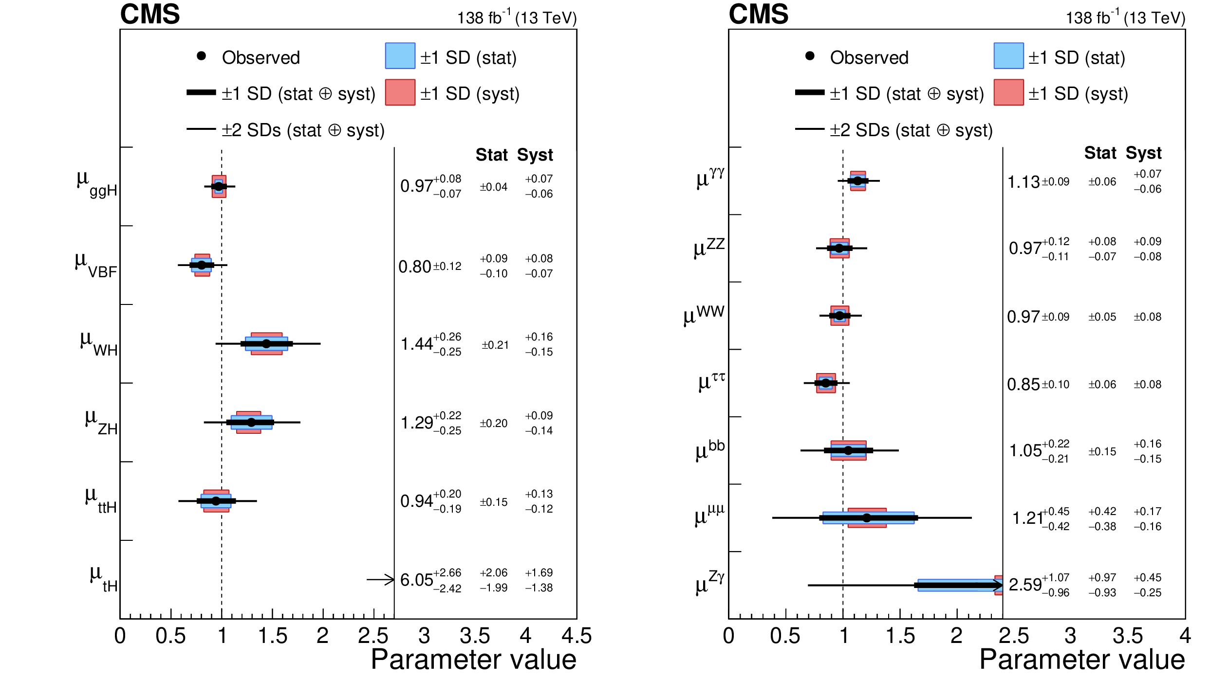
png pdf	Figure 2: Signal strength parameters extracted for various production modes $ \mu_i $, assuming the branching fractions $ \mathcal{B}^f = \mathcal{B}^\text{f}_\text{SM} $ (left), and decay channels $ \mu^\text{f} $, assuming the production cross sections as predicted by the SM (right). The thick and thin black lines indicate the one and two s.d. confidence intervals (labelled by SD in the figures), with the systematic and statistical components of the former indicated by the red and blue bands, respectively. The vertical dashed line at unity represents the values of $ \mu_i $ (resp. $ \mu^\text{f} $) in the SM. Taken from Ref [4].
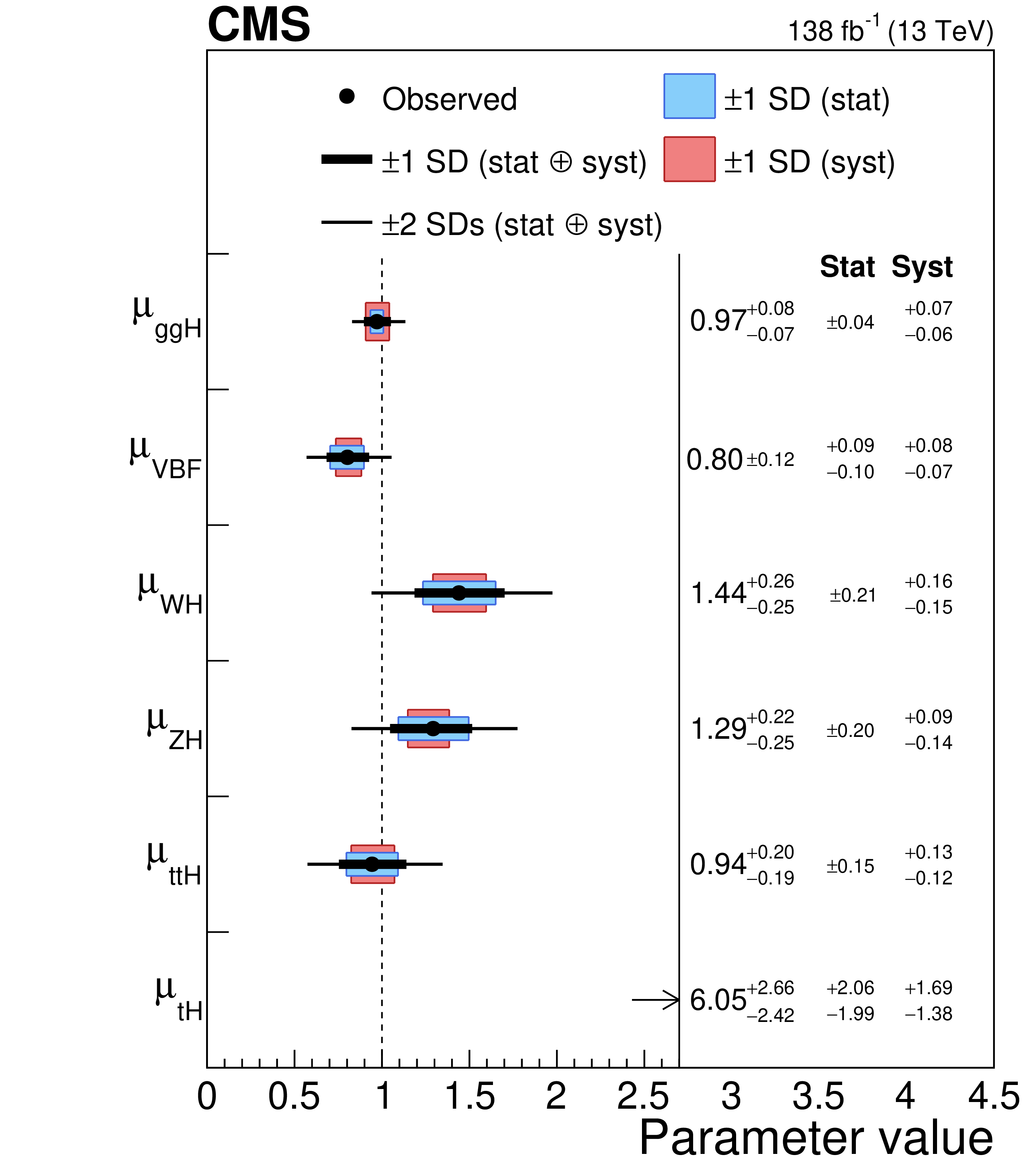
png pdf	Figure 2-a: Signal strength parameters extracted for various production modes $ \mu_i $, assuming the branching fractions $ \mathcal{B}^f = \mathcal{B}^\text{f}_\text{SM} $ (left), and decay channels $ \mu^\text{f} $, assuming the production cross sections as predicted by the SM (right). The thick and thin black lines indicate the one and two s.d. confidence intervals (labelled by SD in the figures), with the systematic and statistical components of the former indicated by the red and blue bands, respectively. The vertical dashed line at unity represents the values of $ \mu_i $ (resp. $ \mu^\text{f} $) in the SM. Taken from Ref [4].
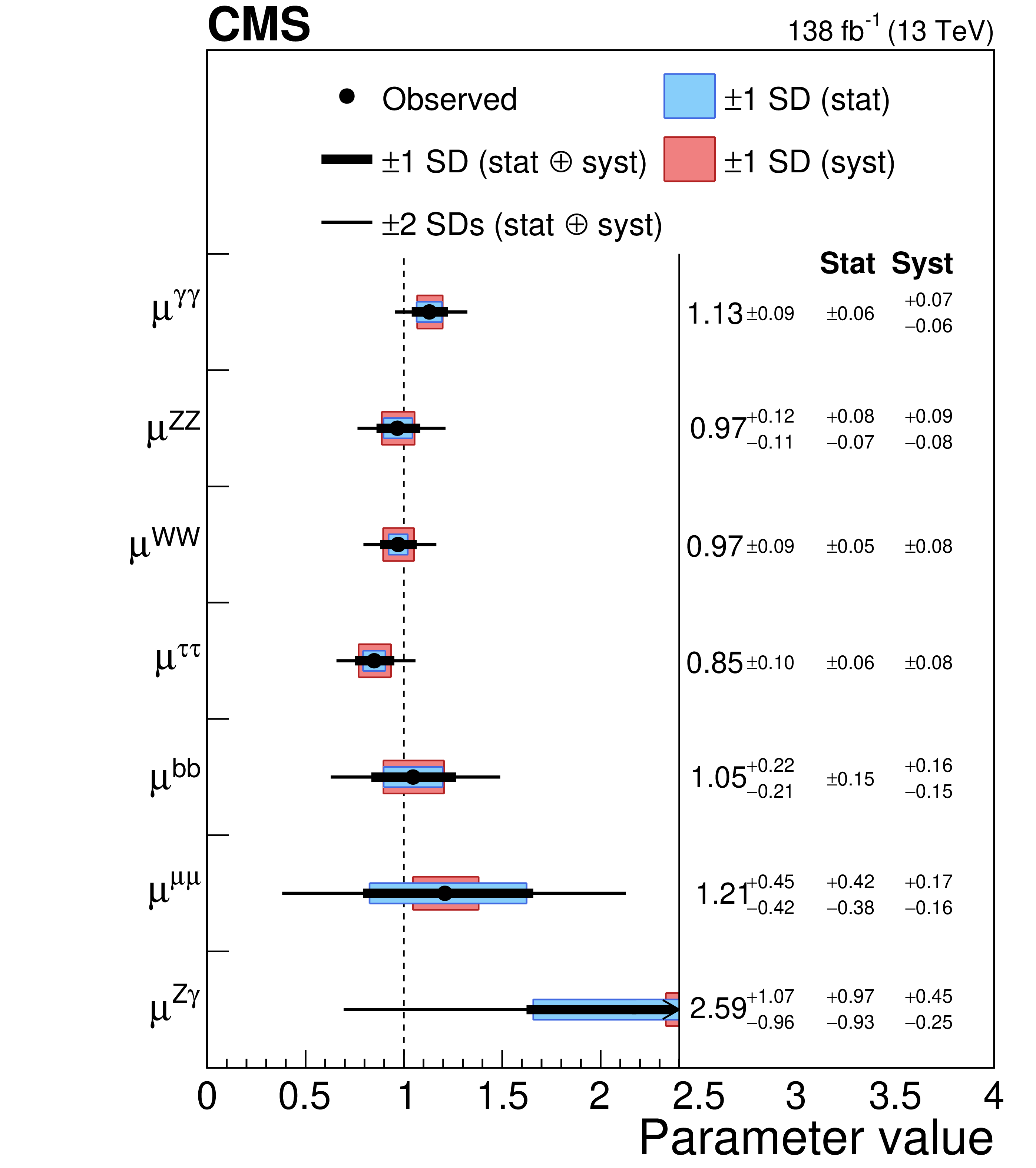
png pdf	Figure 2-b: Signal strength parameters extracted for various production modes $ \mu_i $, assuming the branching fractions $ \mathcal{B}^f = \mathcal{B}^\text{f}_\text{SM} $ (left), and decay channels $ \mu^\text{f} $, assuming the production cross sections as predicted by the SM (right). The thick and thin black lines indicate the one and two s.d. confidence intervals (labelled by SD in the figures), with the systematic and statistical components of the former indicated by the red and blue bands, respectively. The vertical dashed line at unity represents the values of $ \mu_i $ (resp. $ \mu^\text{f} $) in the SM. Taken from Ref [4].
png pdf	Figure 3: Measurements of the coupling modifiers $ \kappa_{i} $, allowing both invisible and undetected decay modes, with the SM value used as an upper bound on both $ \kappa_\mathrm{W} $ and $ \kappa_\mathrm{Z} $. The thick and thin black lines indicate the $ \pm $1 and $ \pm $2 s.d. confidence intervals, respectively, with the systematic and statistical components of the $ \pm $1 s.d. interval indicated by the red and blue bands. The resulting branching fractions for invisible and undetected decay modes are also displayed. Taken from Ref. [4].
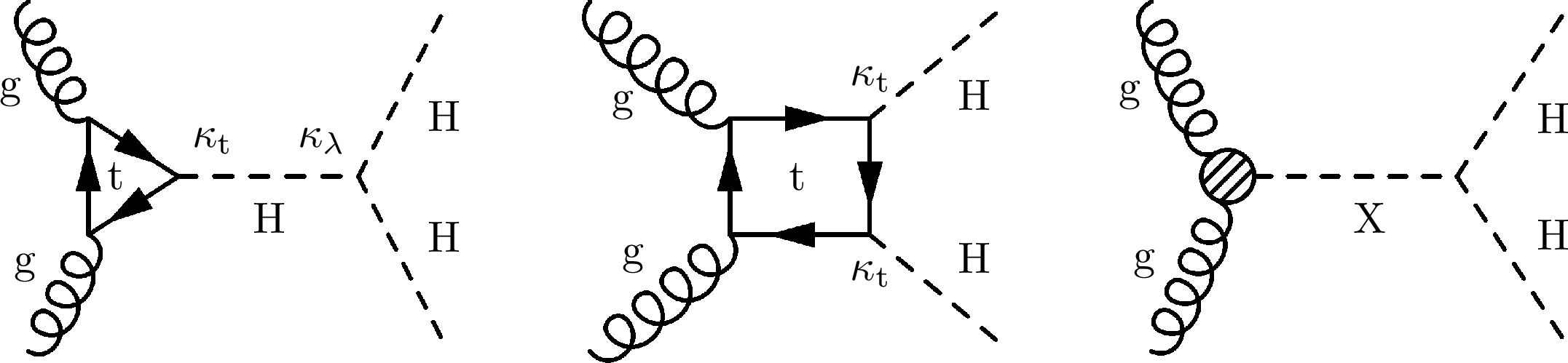
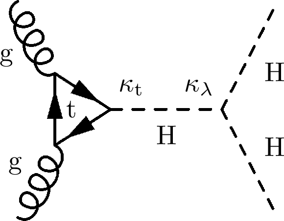
png pdf	Figure 4: Leading order Feynman diagrams of Higgs boson pair production via gluon fusion. The left and middle parts of the figure show the ``triangle'' and ``box'' diagrams, respectively for nonresonant H production, as expected from the SM. The right part of the figure shows a diagram for H boson production through a new resonance of labeled as X.
png pdf	Figure 4-a: Leading order Feynman diagrams of Higgs boson pair production via gluon fusion. The left and middle parts of the figure show the ``triangle'' and ``box'' diagrams, respectively for nonresonant H production, as expected from the SM. The right part of the figure shows a diagram for H boson production through a new resonance of labeled as X.
png pdf	Figure 4-b: Leading order Feynman diagrams of Higgs boson pair production via gluon fusion. The left and middle parts of the figure show the ``triangle'' and ``box'' diagrams, respectively for nonresonant H production, as expected from the SM. The right part of the figure shows a diagram for H boson production through a new resonance of labeled as X.
png pdf	Figure 4-c: Leading order Feynman diagrams of Higgs boson pair production via gluon fusion. The left and middle parts of the figure show the ``triangle'' and ``box'' diagrams, respectively for nonresonant H production, as expected from the SM. The right part of the figure shows a diagram for H boson production through a new resonance of labeled as X.
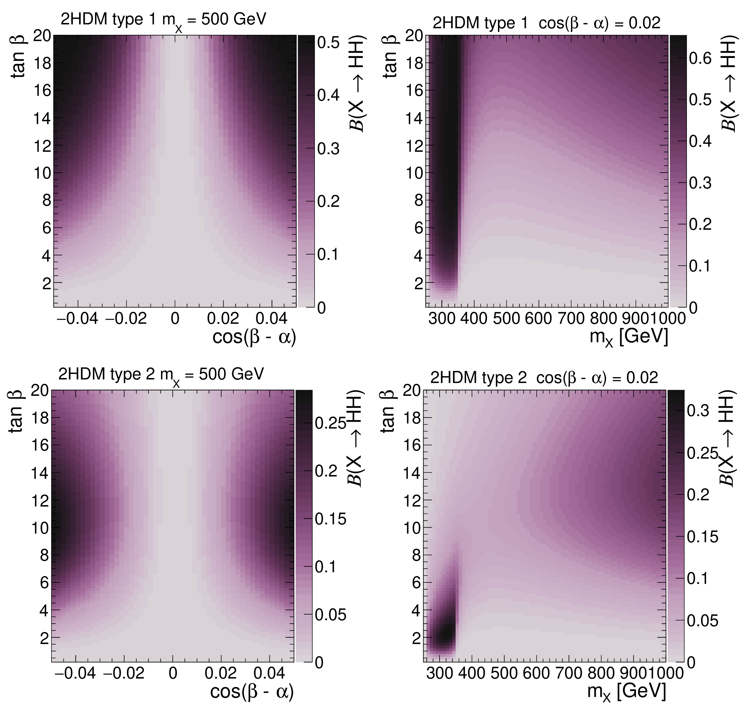
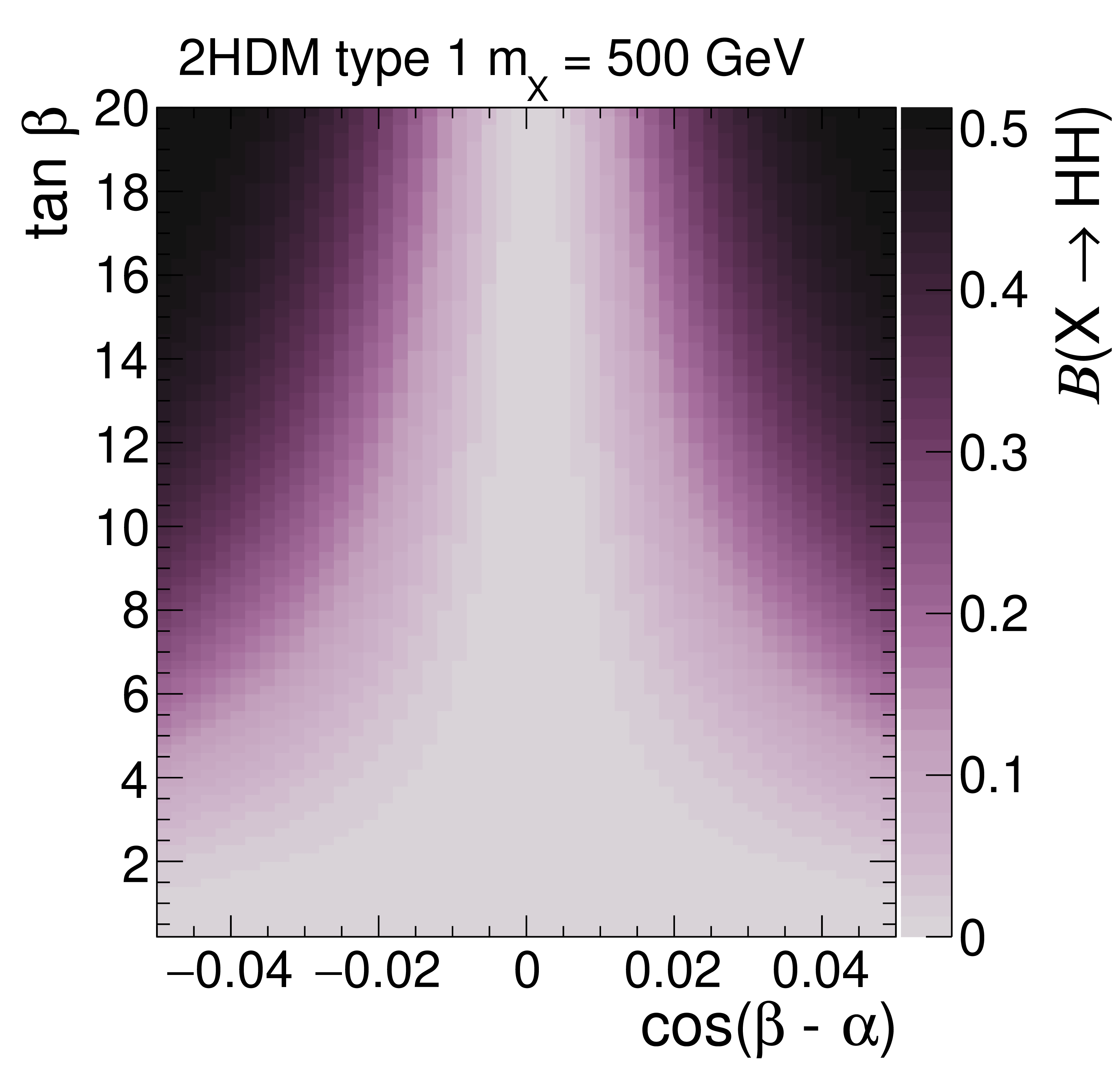
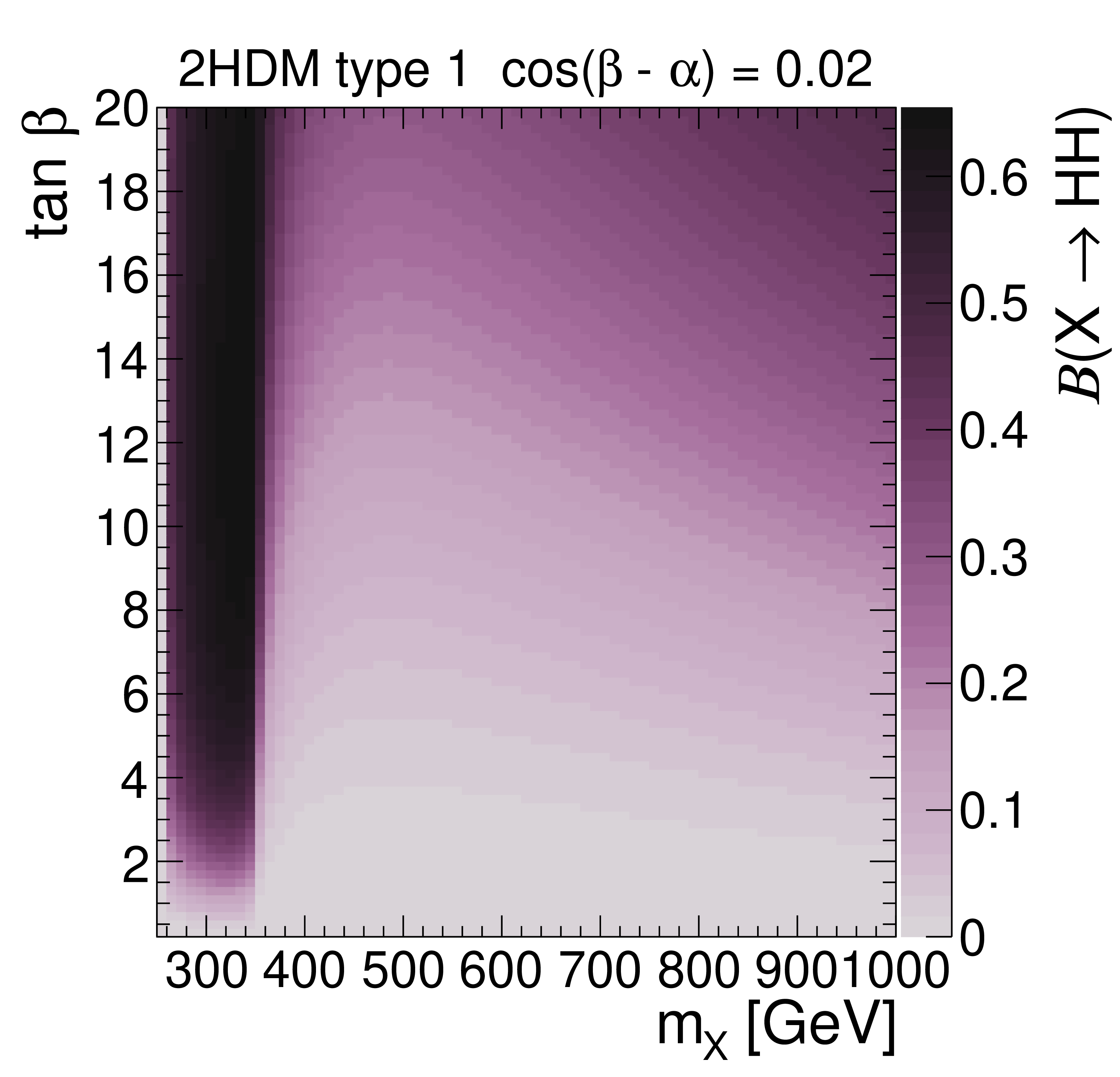
png pdf	Figure 5: Branching fractions of $ \mathrm{X}\to{\mathrm{H}\mathrm{H}} $ decays in 2HDMs of Type I (upper) and Type II (lower) in the $ \cos(\beta - \alpha) $-$ \tan\beta $ plane for $ m_{\mathrm{X}} = $ 500 GeV (left) and in the $ m_{\mathrm{X}} $-$ \tan\beta $ plane for $ \cos(\beta - \alpha) = $ 0.02 (right). The masses of all non-SM-like Higgs bosons are set to be the same, $ m_{\mathrm{X}} = m_{ {\mathrm{A}}} $, and $ m_{12}^2 = m_{{\mathrm{A}}}^2 \tan\beta/(1 + \tan^2\beta) $. The branching fractions have been calculated with 2HDMC v1.8.0 [55, 56].
png pdf	Figure 5-a: Branching fractions of $ \mathrm{X}\to{\mathrm{H}\mathrm{H}} $ decays in 2HDMs of Type I (upper) and Type II (lower) in the $ \cos(\beta - \alpha) $-$ \tan\beta $ plane for $ m_{\mathrm{X}} = $ 500 GeV (left) and in the $ m_{\mathrm{X}} $-$ \tan\beta $ plane for $ \cos(\beta - \alpha) = $ 0.02 (right). The masses of all non-SM-like Higgs bosons are set to be the same, $ m_{\mathrm{X}} = m_{ {\mathrm{A}}} $, and $ m_{12}^2 = m_{{\mathrm{A}}}^2 \tan\beta/(1 + \tan^2\beta) $. The branching fractions have been calculated with 2HDMC v1.8.0 [55, 56].
png pdf	Figure 5-b: Branching fractions of $ \mathrm{X}\to{\mathrm{H}\mathrm{H}} $ decays in 2HDMs of Type I (upper) and Type II (lower) in the $ \cos(\beta - \alpha) $-$ \tan\beta $ plane for $ m_{\mathrm{X}} = $ 500 GeV (left) and in the $ m_{\mathrm{X}} $-$ \tan\beta $ plane for $ \cos(\beta - \alpha) = $ 0.02 (right). The masses of all non-SM-like Higgs bosons are set to be the same, $ m_{\mathrm{X}} = m_{ {\mathrm{A}}} $, and $ m_{12}^2 = m_{{\mathrm{A}}}^2 \tan\beta/(1 + \tan^2\beta) $. The branching fractions have been calculated with 2HDMC v1.8.0 [55, 56].
png pdf	Figure 5-c: Branching fractions of $ \mathrm{X}\to{\mathrm{H}\mathrm{H}} $ decays in 2HDMs of Type I (upper) and Type II (lower) in the $ \cos(\beta - \alpha) $-$ \tan\beta $ plane for $ m_{\mathrm{X}} = $ 500 GeV (left) and in the $ m_{\mathrm{X}} $-$ \tan\beta $ plane for $ \cos(\beta - \alpha) = $ 0.02 (right). The masses of all non-SM-like Higgs bosons are set to be the same, $ m_{\mathrm{X}} = m_{ {\mathrm{A}}} $, and $ m_{12}^2 = m_{{\mathrm{A}}}^2 \tan\beta/(1 + \tan^2\beta) $. The branching fractions have been calculated with 2HDMC v1.8.0 [55, 56].
png pdf	Figure 5-d: Branching fractions of $ \mathrm{X}\to{\mathrm{H}\mathrm{H}} $ decays in 2HDMs of Type I (upper) and Type II (lower) in the $ \cos(\beta - \alpha) $-$ \tan\beta $ plane for $ m_{\mathrm{X}} = $ 500 GeV (left) and in the $ m_{\mathrm{X}} $-$ \tan\beta $ plane for $ \cos(\beta - \alpha) = $ 0.02 (right). The masses of all non-SM-like Higgs bosons are set to be the same, $ m_{\mathrm{X}} = m_{ {\mathrm{A}}} $, and $ m_{12}^2 = m_{{\mathrm{A}}}^2 \tan\beta/(1 + \tan^2\beta) $. The branching fractions have been calculated with 2HDMC v1.8.0 [55, 56].
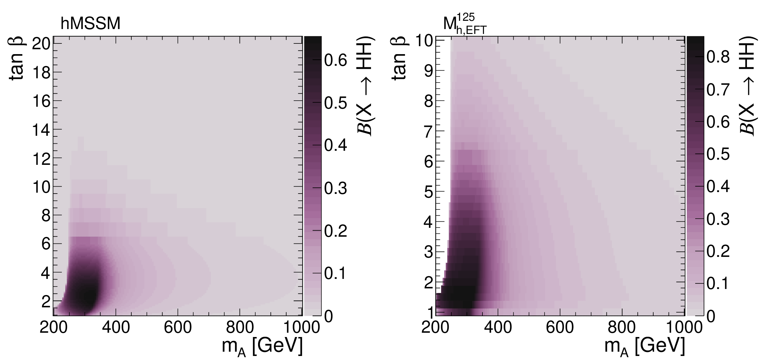
png pdf	Figure 6: Branching fraction of $ \mathrm{X}\to{\mathrm{H}\mathrm{H}} $ decays in the MSSM, for the hMSSM [57,58,59] (left) and the $ M^{125}_{\text{h,EFT}} $ [60] benchmarks, in the $ m_{{\mathrm{A}}} $-$ \tan \beta $ plane. The branching fractions are taken from benchmark files produced by the MSSM subgroup of the LHC Higgs Working Group [61,62].
png pdf	Figure 6-a: Branching fraction of $ \mathrm{X}\to{\mathrm{H}\mathrm{H}} $ decays in the MSSM, for the hMSSM [57,58,59] (left) and the $ M^{125}_{\text{h,EFT}} $ [60] benchmarks, in the $ m_{{\mathrm{A}}} $-$ \tan \beta $ plane. The branching fractions are taken from benchmark files produced by the MSSM subgroup of the LHC Higgs Working Group [61,62].
png pdf	Figure 6-b: Branching fraction of $ \mathrm{X}\to{\mathrm{H}\mathrm{H}} $ decays in the MSSM, for the hMSSM [57,58,59] (left) and the $ M^{125}_{\text{h,EFT}} $ [60] benchmarks, in the $ m_{{\mathrm{A}}} $-$ \tan \beta $ plane. The branching fractions are taken from benchmark files produced by the MSSM subgroup of the LHC Higgs Working Group [61,62].
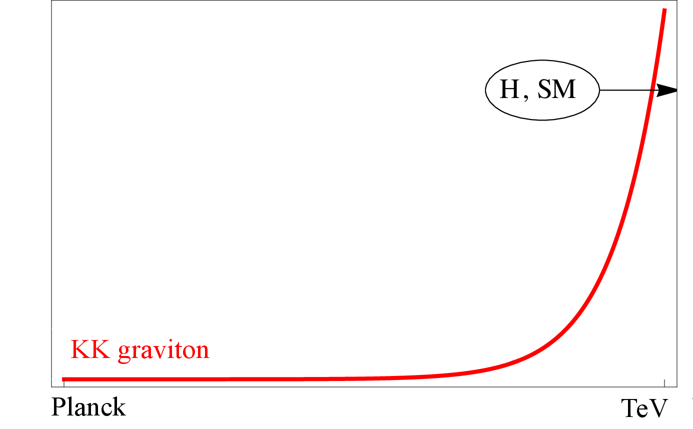
png pdf	Figure 7: Localization of fields on the branes, in different types of the Randall-Sundrum (RS) model: RS1 (left) and bulk-RS (right). The $ x $-axis represents the 5th dimension with the Planck brane on the left and the TeV brane on the right. The $ y $-axis is the probability density. Adapted from Ref. [28].
png pdf	Figure 7-a: Localization of fields on the branes, in different types of the Randall-Sundrum (RS) model: RS1 (left) and bulk-RS (right). The $ x $-axis represents the 5th dimension with the Planck brane on the left and the TeV brane on the right. The $ y $-axis is the probability density. Adapted from Ref. [28].
png pdf	Figure 7-b: Localization of fields on the branes, in different types of the Randall-Sundrum (RS) model: RS1 (left) and bulk-RS (right). The $ x $-axis represents the 5th dimension with the Planck brane on the left and the TeV brane on the right. The $ y $-axis is the probability density. Adapted from Ref. [28].
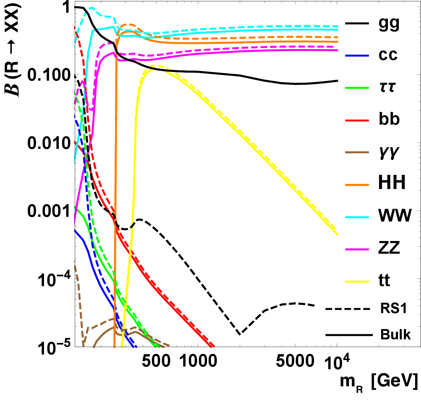
png pdf	Figure 8: The decay branching fractions of an RS1 graviton (top left), bulk graviton (upper right), and radion (lower). Solid lines assume a fully elementary top quark, while the dashed lines ignore the coupling of the graviton to top quarks. Adapted from Ref. [28].
png pdf	Figure 8-a: The decay branching fractions of an RS1 graviton (top left), bulk graviton (upper right), and radion (lower). Solid lines assume a fully elementary top quark, while the dashed lines ignore the coupling of the graviton to top quarks. Adapted from Ref. [28].
png pdf	Figure 8-b: The decay branching fractions of an RS1 graviton (top left), bulk graviton (upper right), and radion (lower). Solid lines assume a fully elementary top quark, while the dashed lines ignore the coupling of the graviton to top quarks. Adapted from Ref. [28].
png pdf	Figure 8-c: The decay branching fractions of an RS1 graviton (top left), bulk graviton (upper right), and radion (lower). Solid lines assume a fully elementary top quark, while the dashed lines ignore the coupling of the graviton to top quarks. Adapted from Ref. [28].
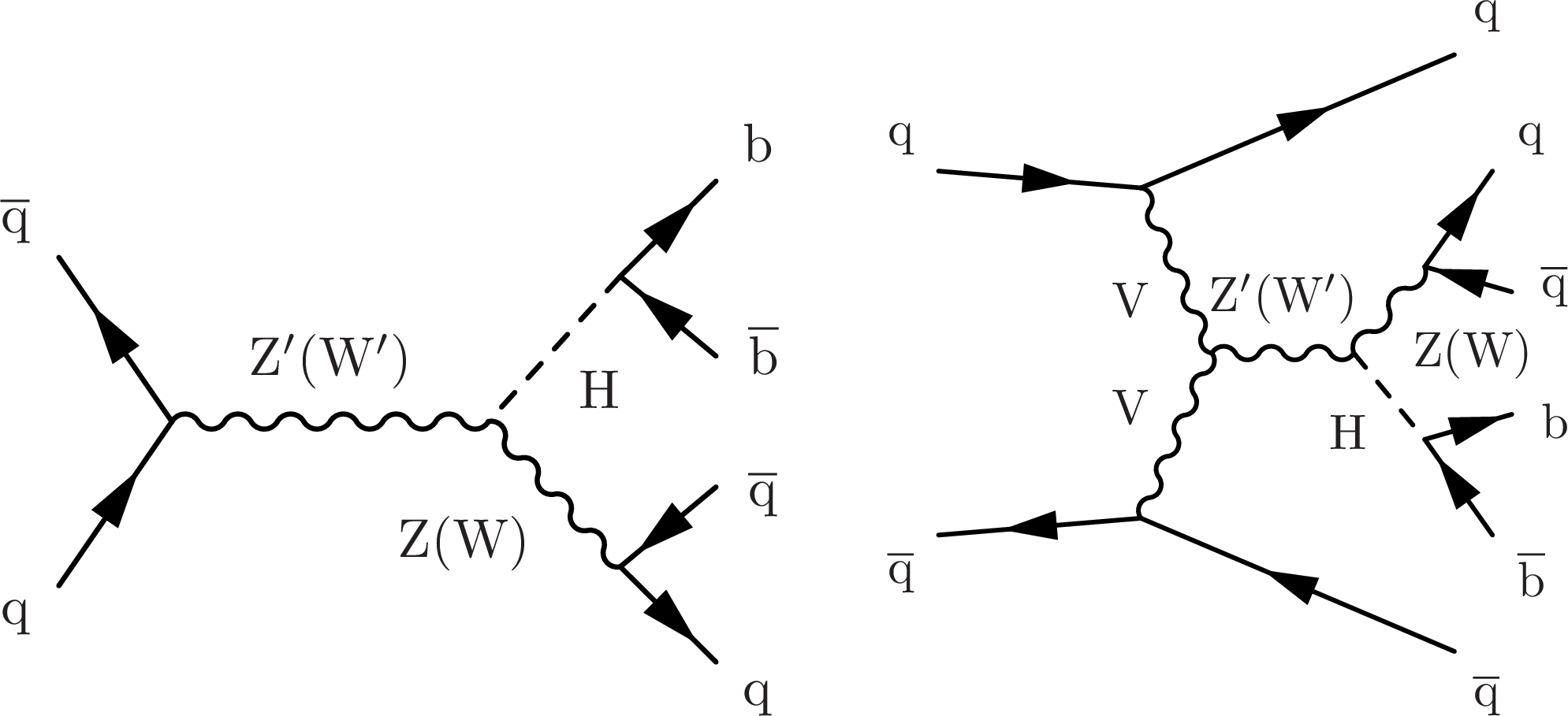
png pdf	Figure 9: Feynman diagrams for the production of Z' and W' bosons produced through the (left) Drell-Yan and (right) vector boson fusion process. The Z' (resp. W') boson subsequently decays into ZH and WH, respectively.
png pdf	Figure 9-a: Feynman diagrams for the production of Z' and W' bosons produced through the (left) Drell-Yan and (right) vector boson fusion process. The Z' (resp. W') boson subsequently decays into ZH and WH, respectively.
png pdf	Figure 9-b: Feynman diagrams for the production of Z' and W' bosons produced through the (left) Drell-Yan and (right) vector boson fusion process. The Z' (resp. W') boson subsequently decays into ZH and WH, respectively.
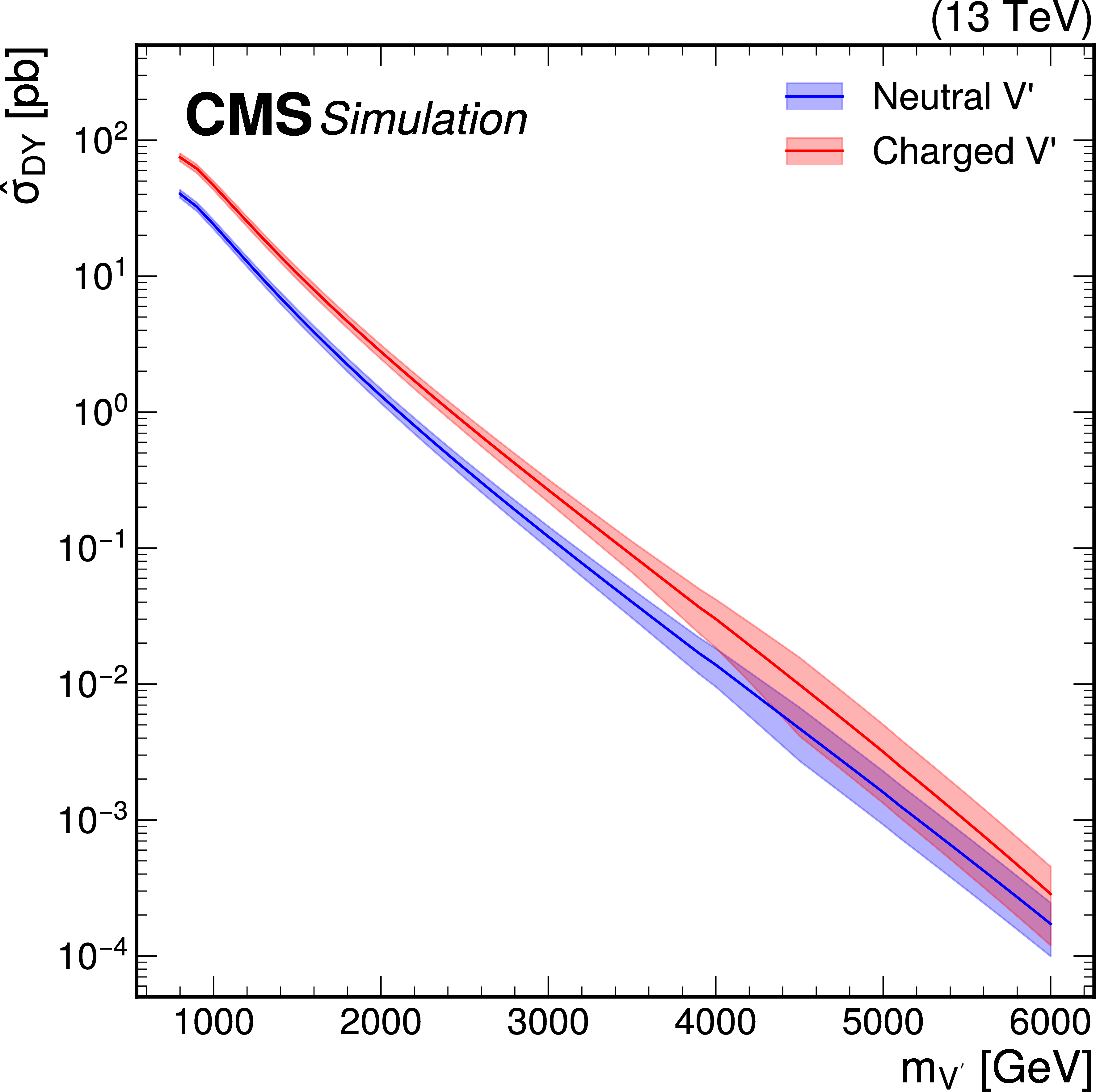
png pdf	Figure 10: Cross sections for (left) Drell-Yan production ($ \hat{\sigma}_{\mathrm{DY}} $) and (right) production through vector boson fusion ($ \hat{\sigma}_{\mathrm{ VBF}} $), as defined in Eqs. \eqrefeq:DY_HVT and \eqrefeq:VBF_HVT, for Z' and W' bosons in the heavy vector triplet (HVT) model B at $ \sqrt{s} = $ 13 TeV. Calculations are based on the work of Ref. [30].
png pdf	Figure 10-a: Cross sections for (left) Drell-Yan production ($ \hat{\sigma}_{\mathrm{DY}} $) and (right) production through vector boson fusion ($ \hat{\sigma}_{\mathrm{ VBF}} $), as defined in Eqs. \eqrefeq:DY_HVT and \eqrefeq:VBF_HVT, for Z' and W' bosons in the heavy vector triplet (HVT) model B at $ \sqrt{s} = $ 13 TeV. Calculations are based on the work of Ref. [30].
png pdf	Figure 10-b: Cross sections for (left) Drell-Yan production ($ \hat{\sigma}_{\mathrm{DY}} $) and (right) production through vector boson fusion ($ \hat{\sigma}_{\mathrm{ VBF}} $), as defined in Eqs. \eqrefeq:DY_HVT and \eqrefeq:VBF_HVT, for Z' and W' bosons in the heavy vector triplet (HVT) model B at $ \sqrt{s} = $ 13 TeV. Calculations are based on the work of Ref. [30].
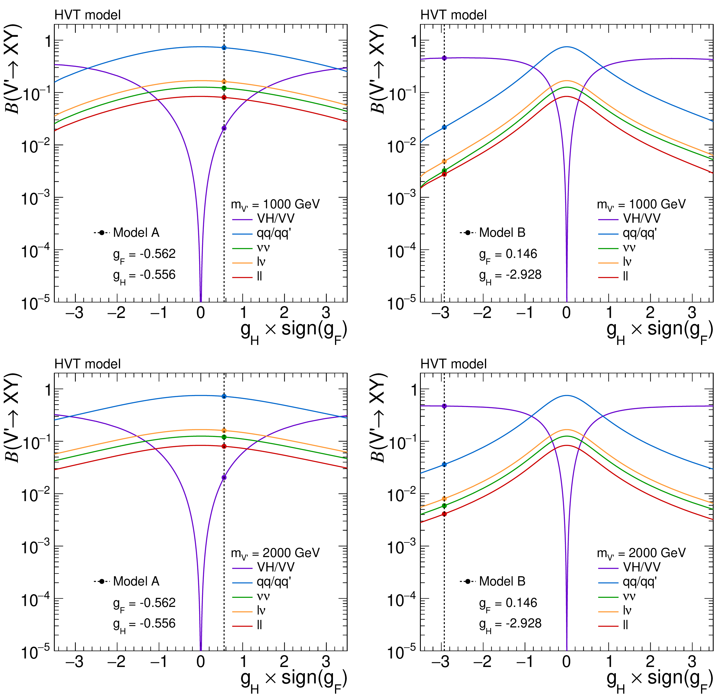
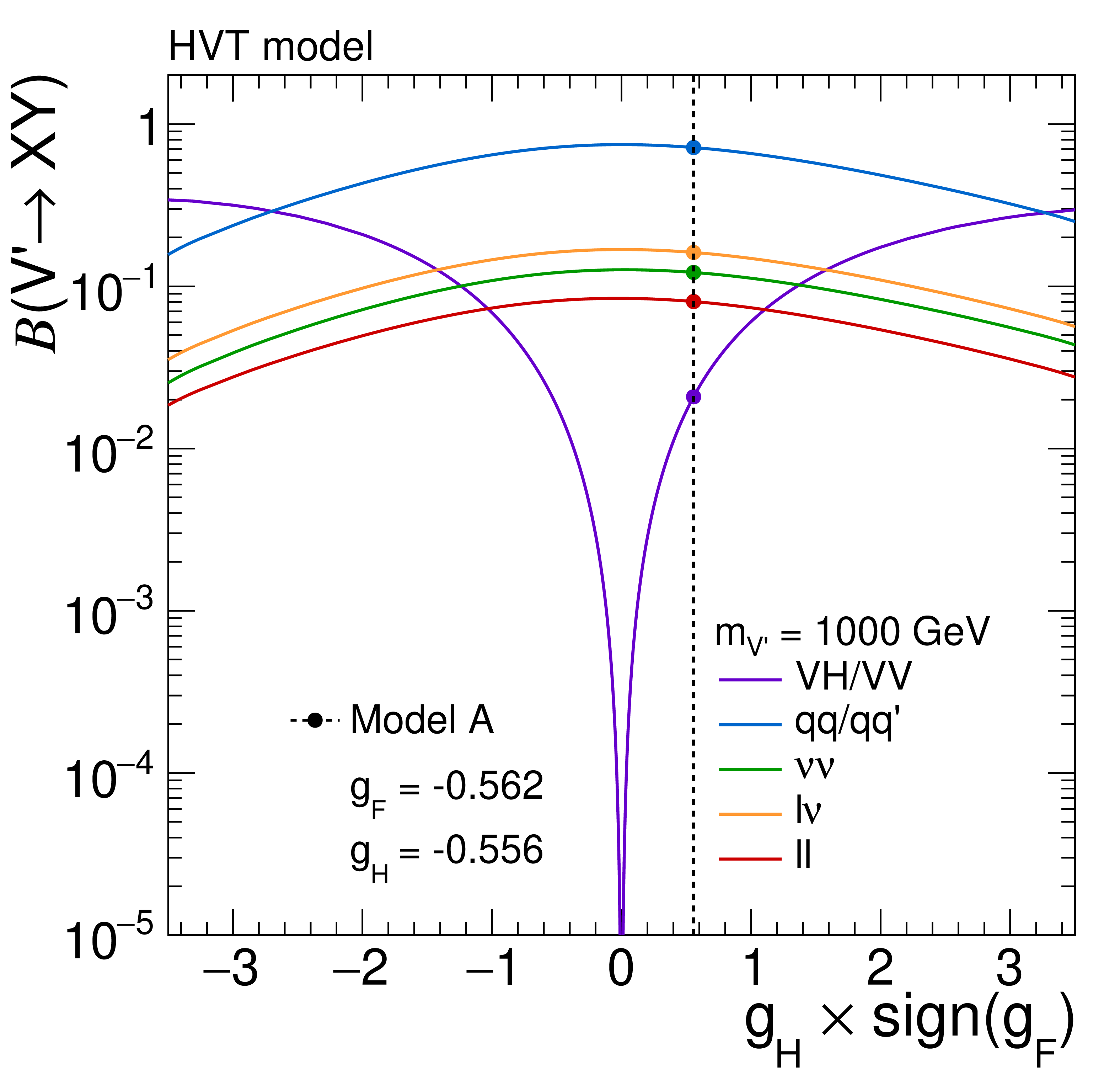
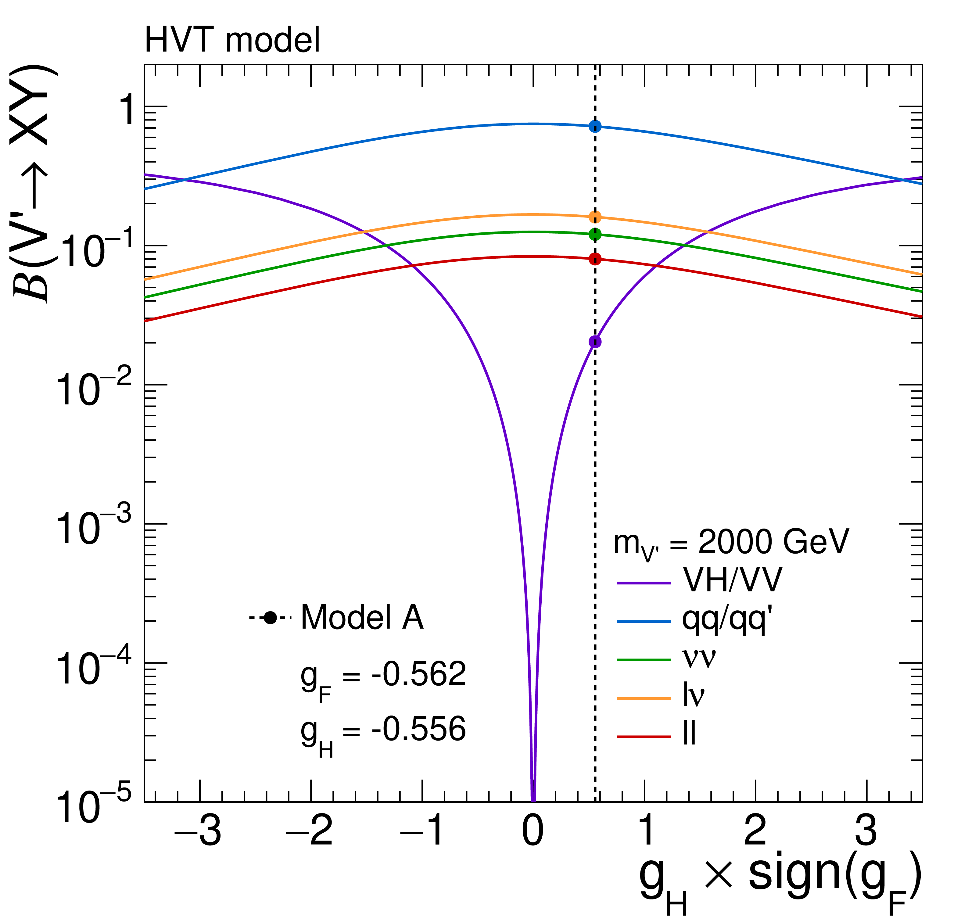
png pdf	Figure 11: Branching fractions for heavy vector triplet (HVT) bosons with masses of (upper) 1 and (lower) 2 TeV for values of the parameter $ g_\mathrm{F} $ corresponding to models (left) A and (right) B. The exact branching fractions of each model are indicated by the crossing points of the individual curves with the dashed vertical lines. Calculations are based on the work of Ref. [30].
png pdf	Figure 11-a: Branching fractions for heavy vector triplet (HVT) bosons with masses of (upper) 1 and (lower) 2 TeV for values of the parameter $ g_\mathrm{F} $ corresponding to models (left) A and (right) B. The exact branching fractions of each model are indicated by the crossing points of the individual curves with the dashed vertical lines. Calculations are based on the work of Ref. [30].
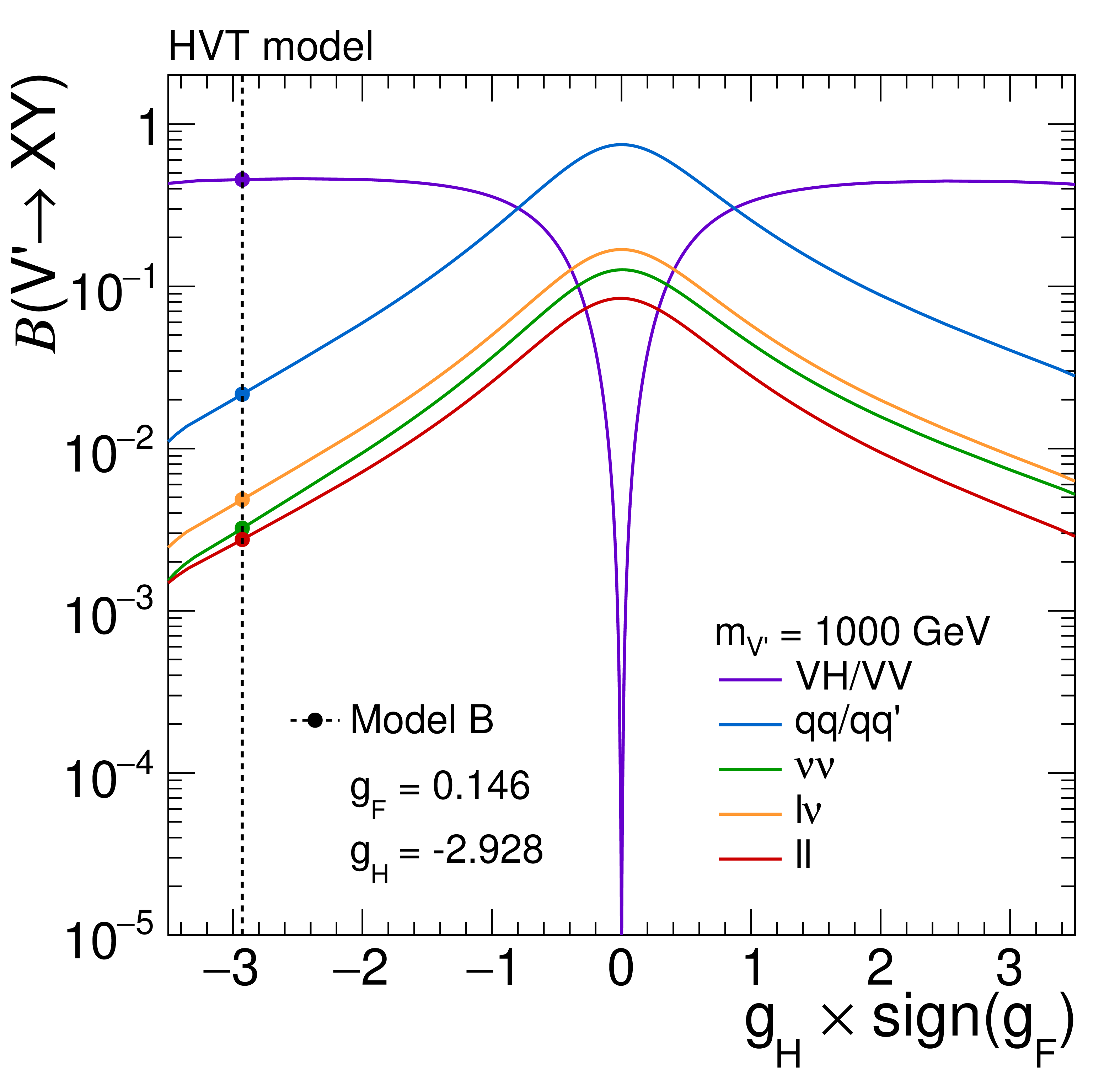
png pdf	Figure 11-b: Branching fractions for heavy vector triplet (HVT) bosons with masses of (upper) 1 and (lower) 2 TeV for values of the parameter $ g_\mathrm{F} $ corresponding to models (left) A and (right) B. The exact branching fractions of each model are indicated by the crossing points of the individual curves with the dashed vertical lines. Calculations are based on the work of Ref. [30].
png pdf	Figure 11-c: Branching fractions for heavy vector triplet (HVT) bosons with masses of (upper) 1 and (lower) 2 TeV for values of the parameter $ g_\mathrm{F} $ corresponding to models (left) A and (right) B. The exact branching fractions of each model are indicated by the crossing points of the individual curves with the dashed vertical lines. Calculations are based on the work of Ref. [30].
png pdf	Figure 11-d: Branching fractions for heavy vector triplet (HVT) bosons with masses of (upper) 1 and (lower) 2 TeV for values of the parameter $ g_\mathrm{F} $ corresponding to models (left) A and (right) B. The exact branching fractions of each model are indicated by the crossing points of the individual curves with the dashed vertical lines. Calculations are based on the work of Ref. [30].
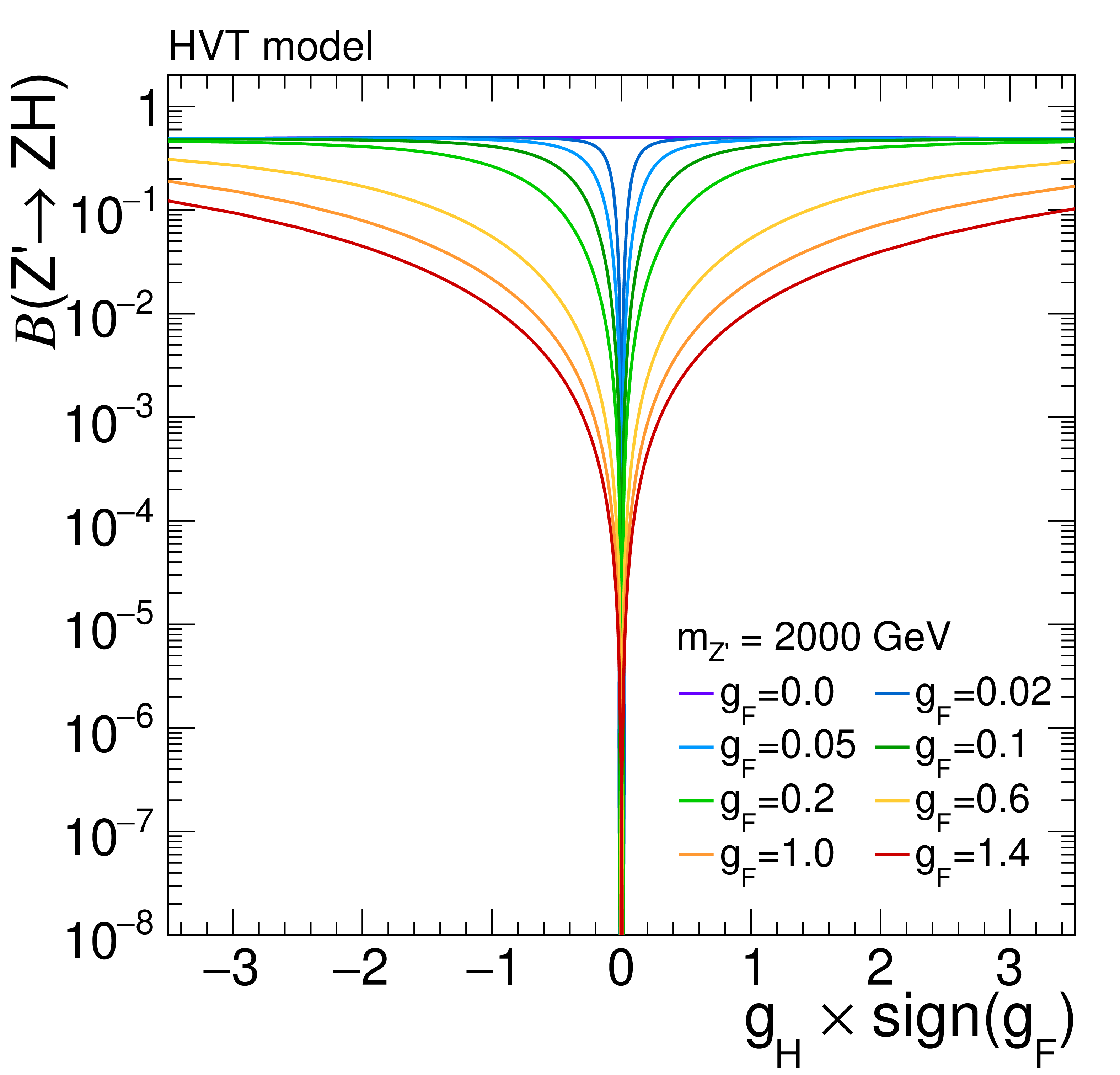
png pdf	Figure 12: (left) Branching fraction for the decay $ \mathrm{Z}^{'}\to\mathrm{Z}\mathrm{H} $, and (right) total width of the Z' boson, for a resonance with 2 TeV mass, for different values of the parameter $ g_\mathrm{F} $. Calculations are based the work of Ref. [30].
png pdf	Figure 12-a: (left) Branching fraction for the decay $ \mathrm{Z}^{'}\to\mathrm{Z}\mathrm{H} $, and (right) total width of the Z' boson, for a resonance with 2 TeV mass, for different values of the parameter $ g_\mathrm{F} $. Calculations are based the work of Ref. [30].
png pdf	Figure 12-b: (left) Branching fraction for the decay $ \mathrm{Z}^{'}\to\mathrm{Z}\mathrm{H} $, and (right) total width of the Z' boson, for a resonance with 2 TeV mass, for different values of the parameter $ g_\mathrm{F} $. Calculations are based the work of Ref. [30].
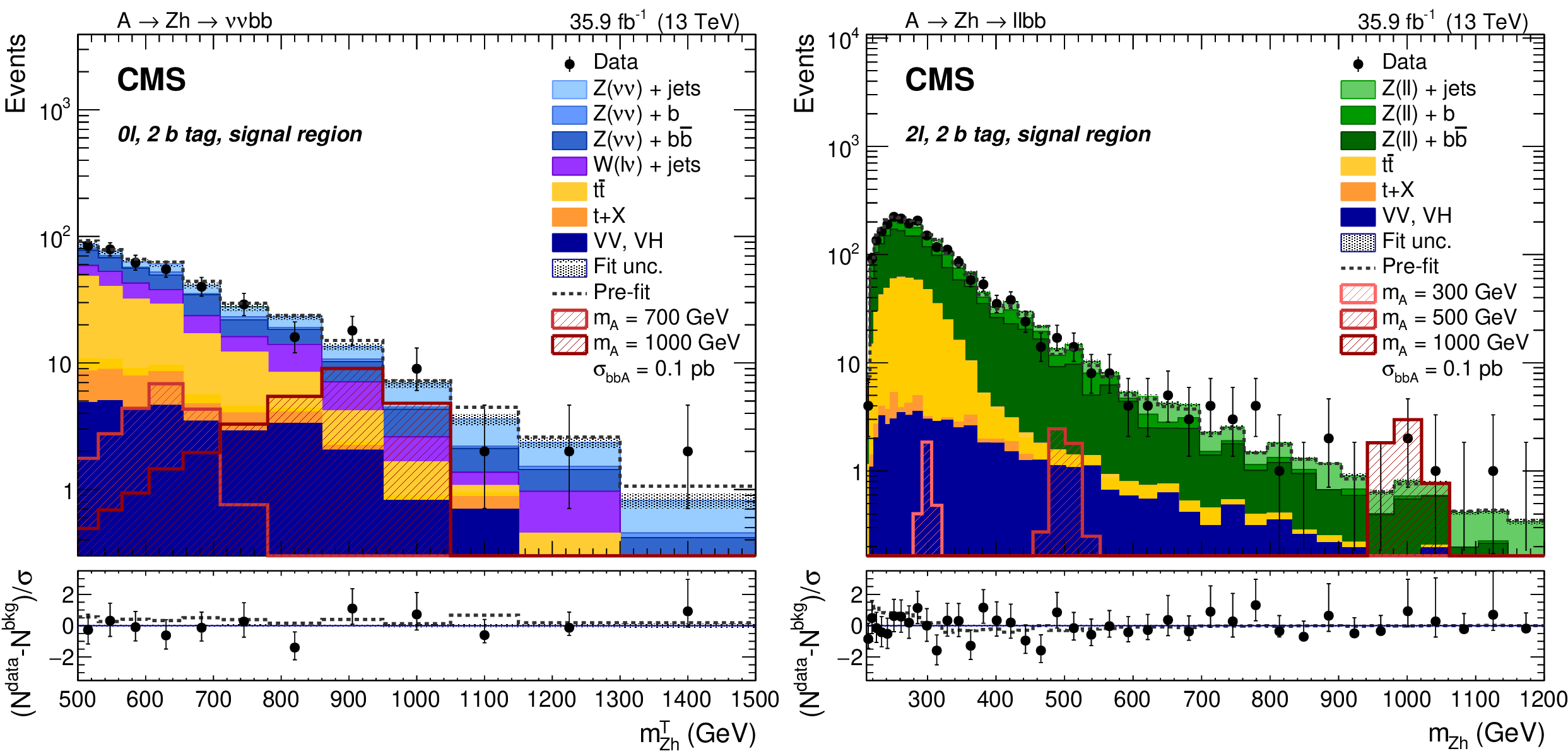
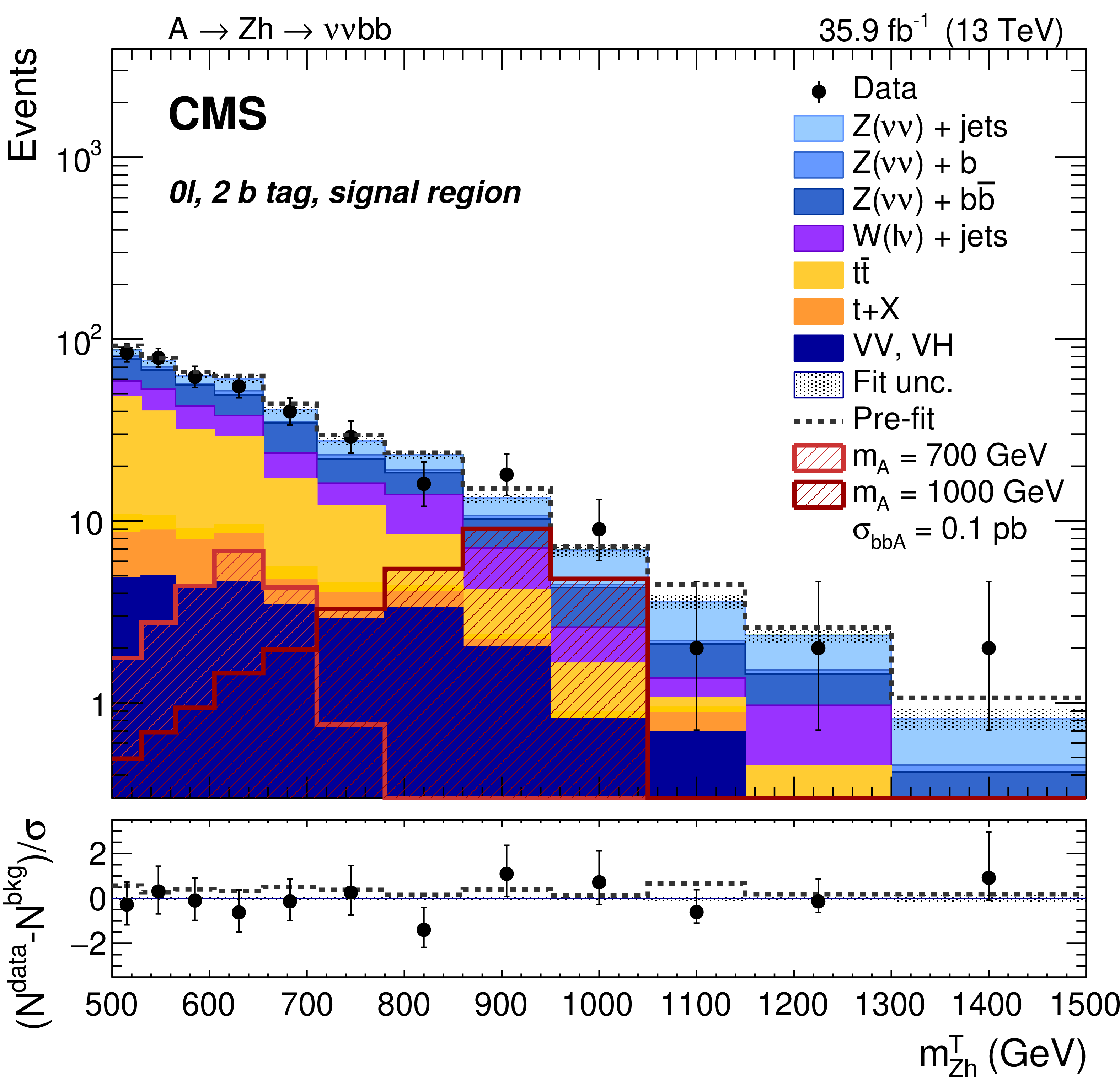
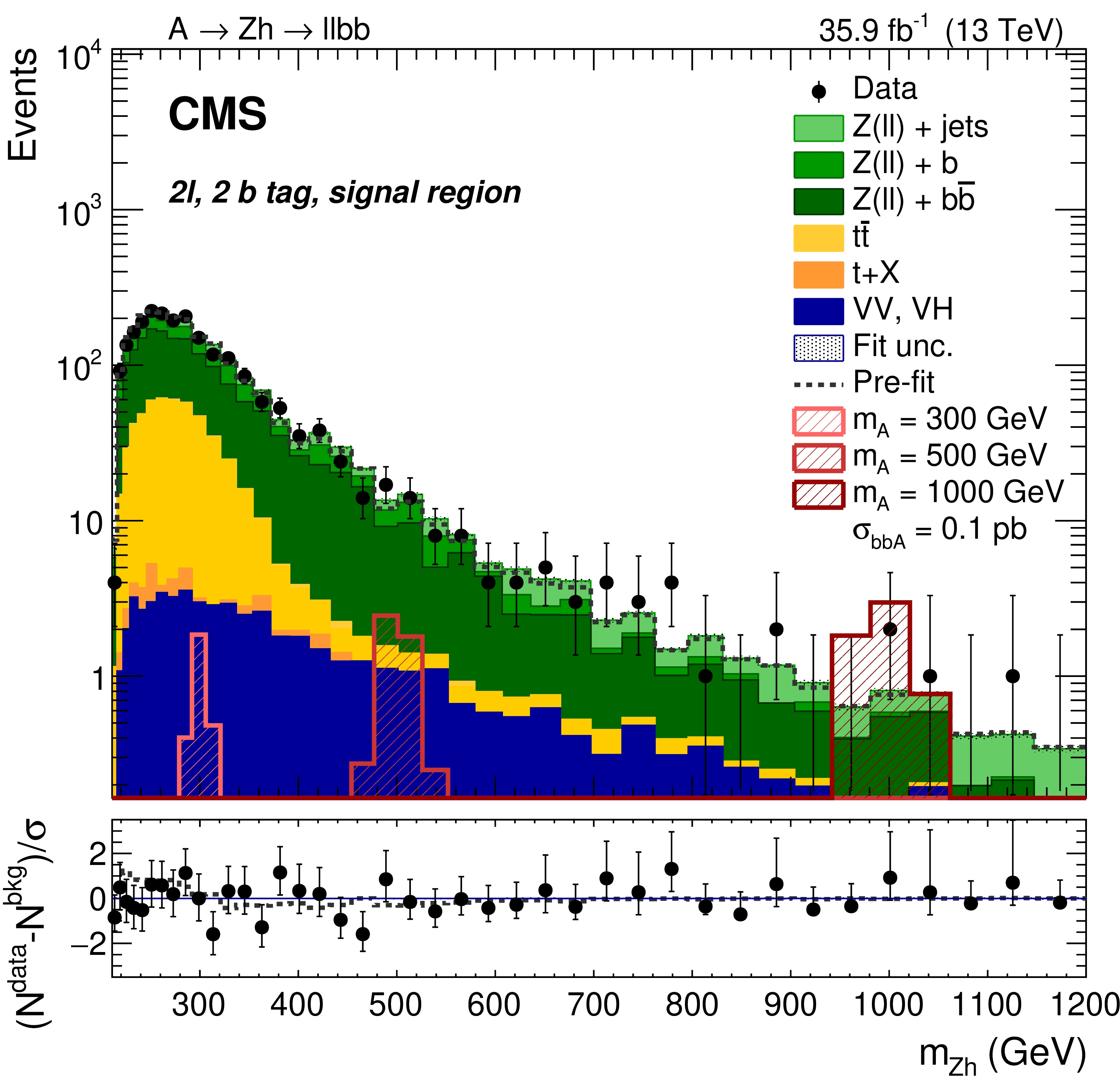
png pdf	Figure 13: Search for $ \mathrm{X}\to\mathrm{V}\mathrm{H}(\mathrm{b}\mathrm{b}) $: Distributions of the $ m_{\mathrm{Z}\mathrm{H}}^{\text{T}} $ and $ m_{\mathrm{Z}\mathrm{H}} $ variables, as introduced in the text, in the (left) 0 $ \ell $ and (right) 2 $ \ell $ categories, in the 2 b tag signal region of the $ {\mathrm{A}} \to\mathrm{Z}\mathrm{H}(\mathrm{b}\mathrm{b}) $ analysis [108]. In the 2 $ \ell $ categories, the contributions of the 2 e and 2 $ \mu $ channels have been summed. The gray dotted line represents the sum of all background processes before the fit to data; the shaded area represents the post-fit uncertainty. The hatched red histograms represent signal hypotheses for b quark associated X production corresponding to $ \sigma_{{\mathrm{A}} }\mathcal{B}({\mathrm{A}} \to\mathrm{Z}\mathrm{H}) \mathcal{B}(\mathrm{H}\to\mathrm{b}\mathrm{b})= $ 0.1 pb. The lower panels depict $ (N^\text{ data}-N^\text{bkg})/\sigma $ in each bin, where $ \sigma $ refers to the statistical uncertainty in the given bin. Figure from Ref. [108].
png pdf	Figure 13-a: Search for $ \mathrm{X}\to\mathrm{V}\mathrm{H}(\mathrm{b}\mathrm{b}) $: Distributions of the $ m_{\mathrm{Z}\mathrm{H}}^{\text{T}} $ and $ m_{\mathrm{Z}\mathrm{H}} $ variables, as introduced in the text, in the (left) 0 $ \ell $ and (right) 2 $ \ell $ categories, in the 2 b tag signal region of the $ {\mathrm{A}} \to\mathrm{Z}\mathrm{H}(\mathrm{b}\mathrm{b}) $ analysis [108]. In the 2 $ \ell $ categories, the contributions of the 2 e and 2 $ \mu $ channels have been summed. The gray dotted line represents the sum of all background processes before the fit to data; the shaded area represents the post-fit uncertainty. The hatched red histograms represent signal hypotheses for b quark associated X production corresponding to $ \sigma_{{\mathrm{A}} }\mathcal{B}({\mathrm{A}} \to\mathrm{Z}\mathrm{H}) \mathcal{B}(\mathrm{H}\to\mathrm{b}\mathrm{b})= $ 0.1 pb. The lower panels depict $ (N^\text{ data}-N^\text{bkg})/\sigma $ in each bin, where $ \sigma $ refers to the statistical uncertainty in the given bin. Figure from Ref. [108].
png pdf	Figure 13-b: Search for $ \mathrm{X}\to\mathrm{V}\mathrm{H}(\mathrm{b}\mathrm{b}) $: Distributions of the $ m_{\mathrm{Z}\mathrm{H}}^{\text{T}} $ and $ m_{\mathrm{Z}\mathrm{H}} $ variables, as introduced in the text, in the (left) 0 $ \ell $ and (right) 2 $ \ell $ categories, in the 2 b tag signal region of the $ {\mathrm{A}} \to\mathrm{Z}\mathrm{H}(\mathrm{b}\mathrm{b}) $ analysis [108]. In the 2 $ \ell $ categories, the contributions of the 2 e and 2 $ \mu $ channels have been summed. The gray dotted line represents the sum of all background processes before the fit to data; the shaded area represents the post-fit uncertainty. The hatched red histograms represent signal hypotheses for b quark associated X production corresponding to $ \sigma_{{\mathrm{A}} }\mathcal{B}({\mathrm{A}} \to\mathrm{Z}\mathrm{H}) \mathcal{B}(\mathrm{H}\to\mathrm{b}\mathrm{b})= $ 0.1 pb. The lower panels depict $ (N^\text{ data}-N^\text{bkg})/\sigma $ in each bin, where $ \sigma $ refers to the statistical uncertainty in the given bin. Figure from Ref. [108].
png pdf	Figure 14: Search for $ \mathrm{X}\to\mathrm{V}\mathrm{H}(\tau\tau) $: Distribution of the $ m_{\ell\ell\tau\tau}^{\mathrm{c}} $ variable, as introduced in the text, of the $ {\mathrm{A}} \to\mathrm{Z}\mathrm{H}(\tau\tau) $ analysis [107], after a fit of the background-only hypothesis in all eight final states. While the fit is based on corresponding distributions, for each final state individually, these have been combined into a single distribution, for visualization purposes for this figure. Uncertainties include both statistical and systematic components. The expected contribution from the $ {\mathrm{A}}\to\mathrm{Z}\mathrm{H} $ signal process is shown for a pseudoscalar Higgs boson with $ m_{{\mathrm{A}}} = $ 300 GeV with the product of the cross section and branching fraction of 20 fb. Figure from Ref. [107].
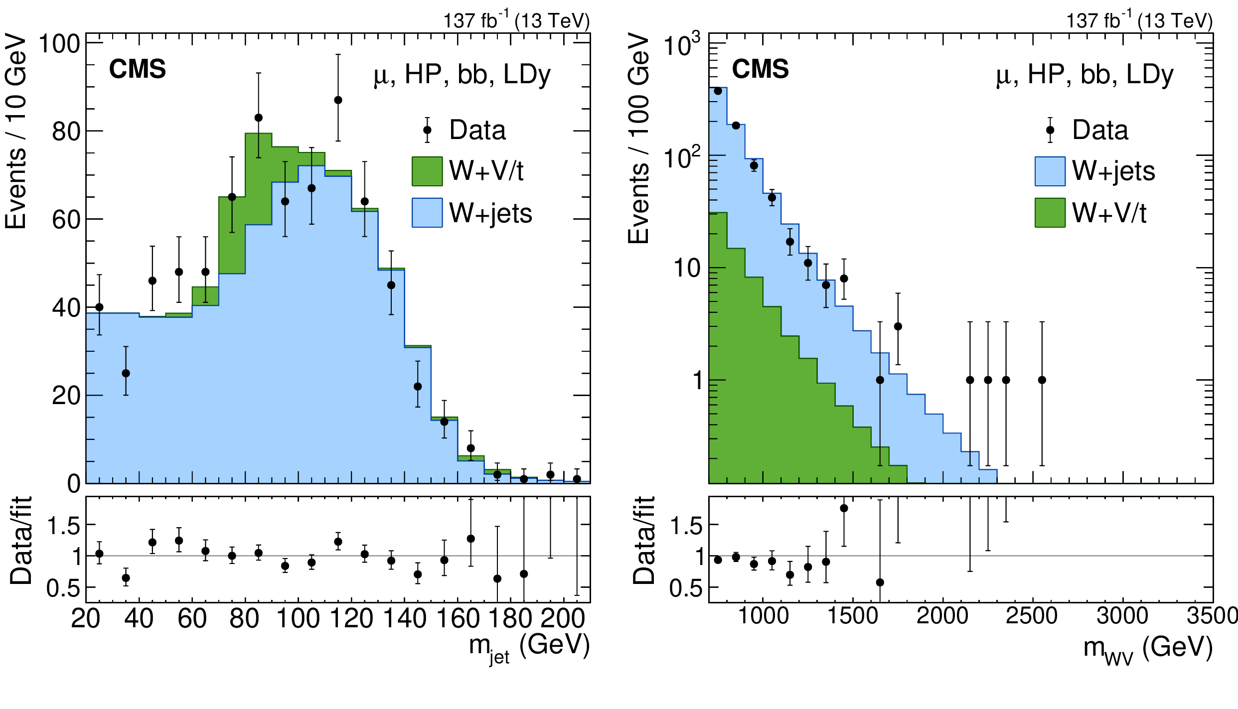
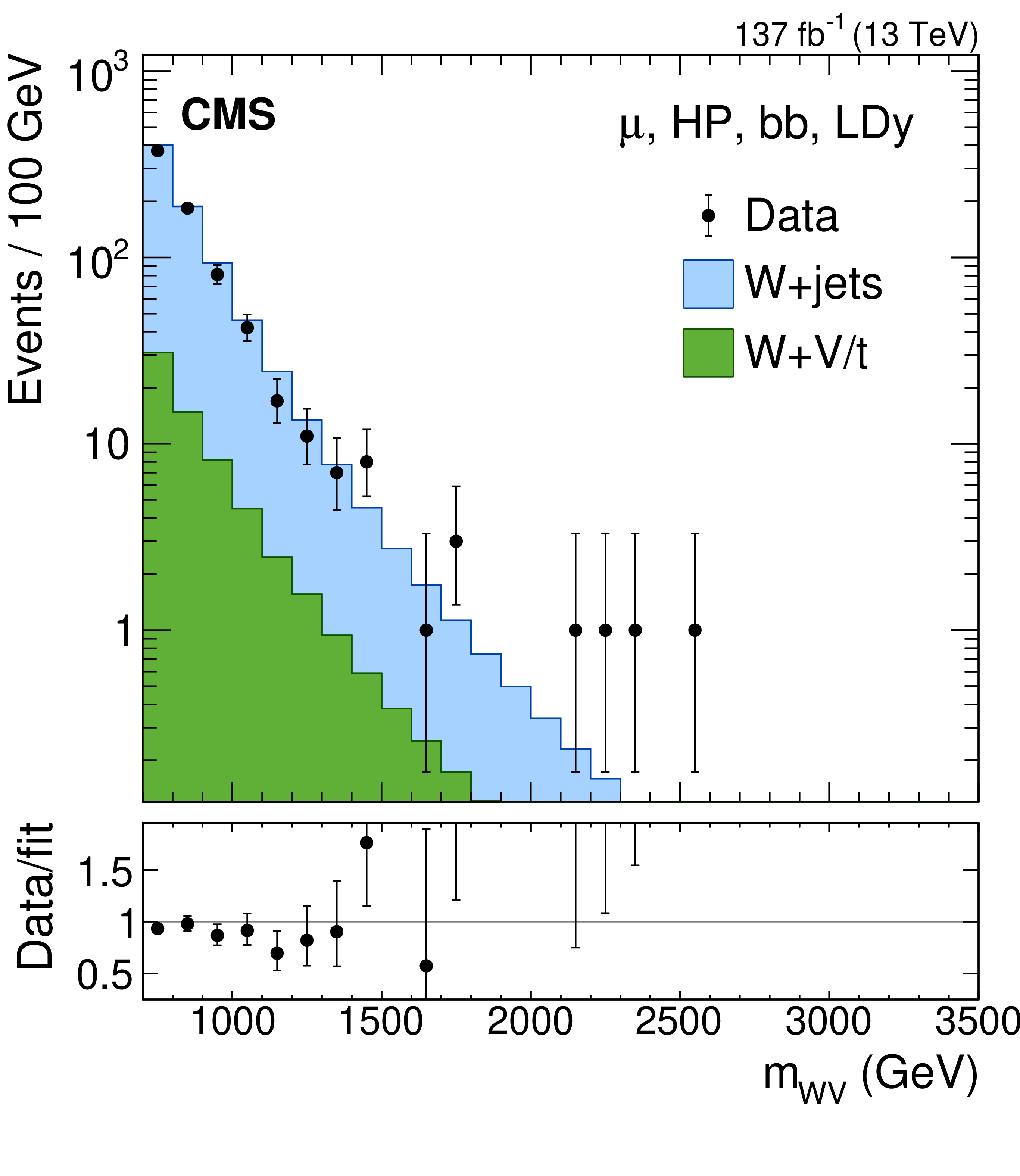
png pdf	Figure 15: Search for $ \mathrm{X}\to\mathrm{V}\mathrm{H}(\mathrm{b}\mathrm{b}) $: Distributions of (left) the jet soft drop mass of a boosted Higgs boson candidate, labeled $ m_{\mathrm{jet}} $, and (right) the mass of the X resonance candidate, labeled $ m_{\mathrm{WV}} $ in the $ \mathrm{W}(\ell\nu)\mathrm{H}(\mathrm{b}\mathrm{b}) $ channel. The notation $ m_{\mathrm{WV}} $ is used as a shorthand since the analysis also searches for resonances in the WW and WZ final states. Figures from Ref. [109].
png pdf	Figure 15-a: Search for $ \mathrm{X}\to\mathrm{V}\mathrm{H}(\mathrm{b}\mathrm{b}) $: Distributions of (left) the jet soft drop mass of a boosted Higgs boson candidate, labeled $ m_{\mathrm{jet}} $, and (right) the mass of the X resonance candidate, labeled $ m_{\mathrm{WV}} $ in the $ \mathrm{W}(\ell\nu)\mathrm{H}(\mathrm{b}\mathrm{b}) $ channel. The notation $ m_{\mathrm{WV}} $ is used as a shorthand since the analysis also searches for resonances in the WW and WZ final states. Figures from Ref. [109].
png pdf	Figure 15-b: Search for $ \mathrm{X}\to\mathrm{V}\mathrm{H}(\mathrm{b}\mathrm{b}) $: Distributions of (left) the jet soft drop mass of a boosted Higgs boson candidate, labeled $ m_{\mathrm{jet}} $, and (right) the mass of the X resonance candidate, labeled $ m_{\mathrm{WV}} $ in the $ \mathrm{W}(\ell\nu)\mathrm{H}(\mathrm{b}\mathrm{b}) $ channel. The notation $ m_{\mathrm{WV}} $ is used as a shorthand since the analysis also searches for resonances in the WW and WZ final states. Figures from Ref. [109].
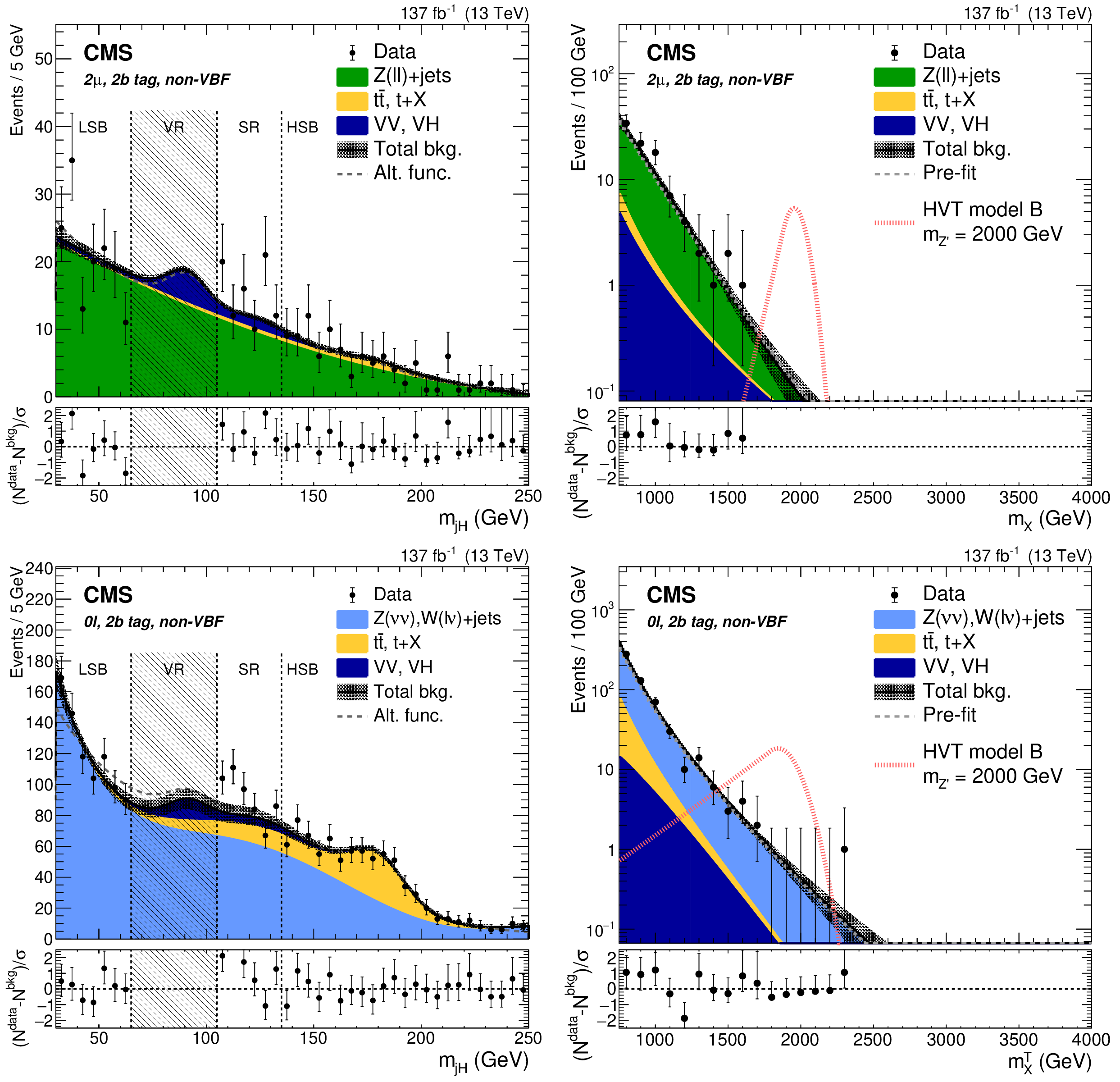
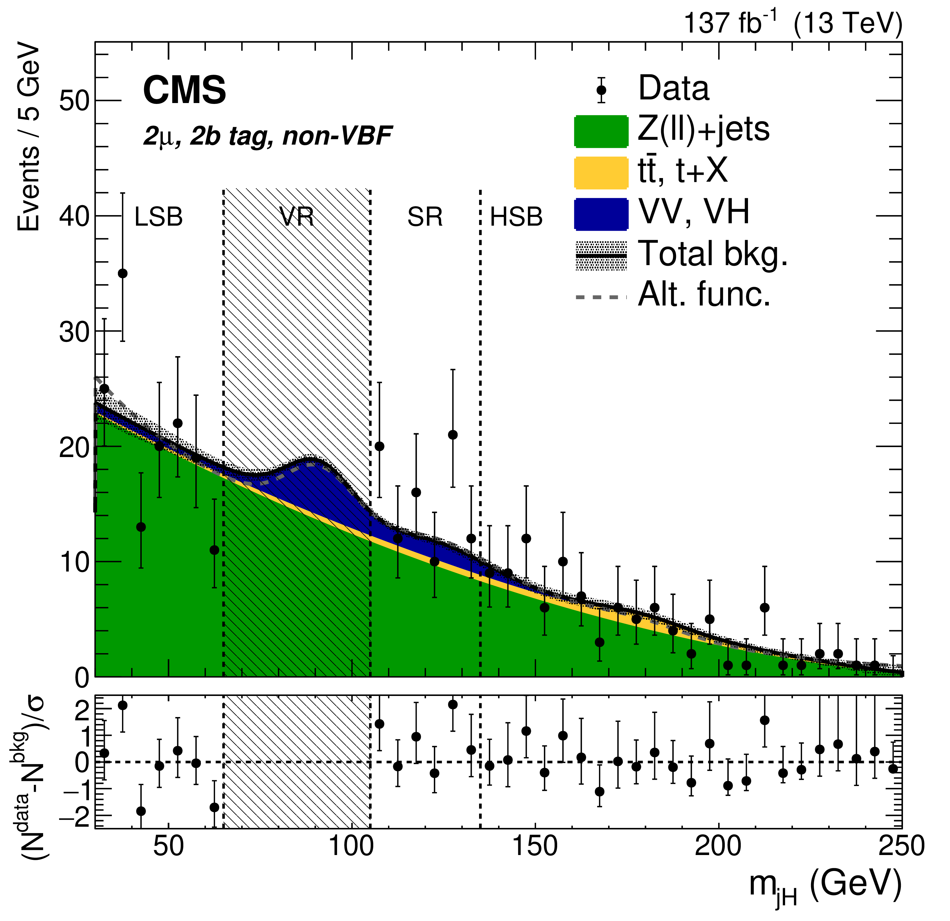
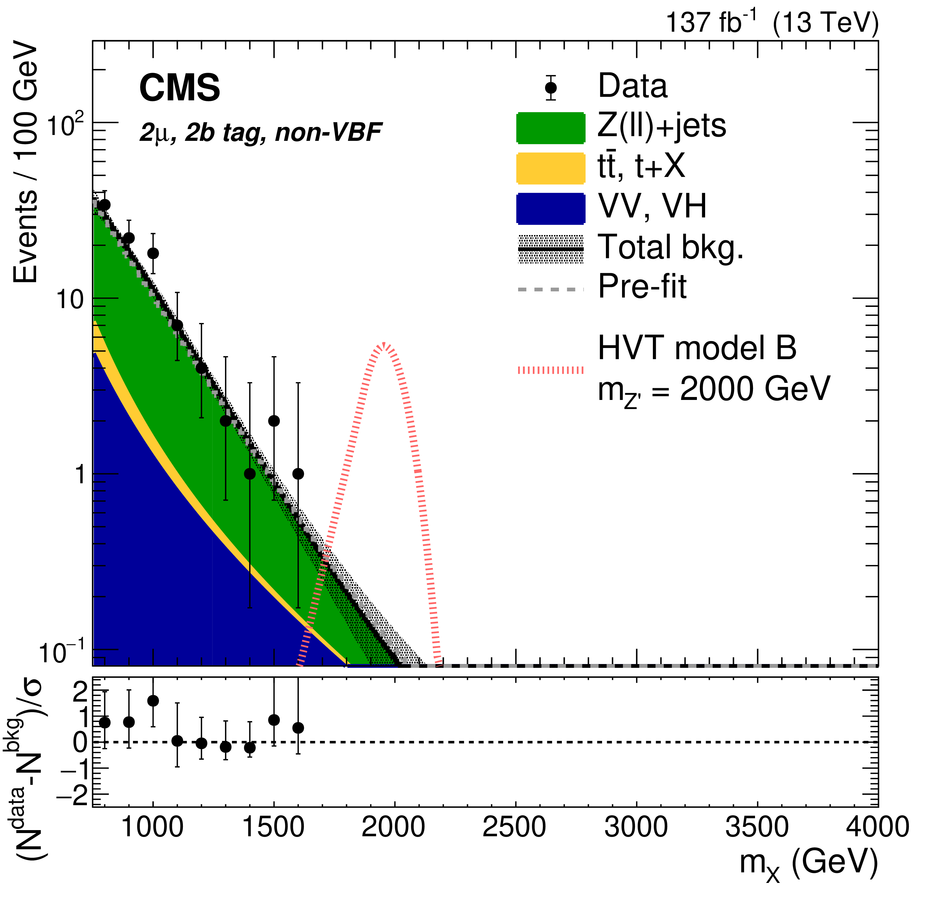
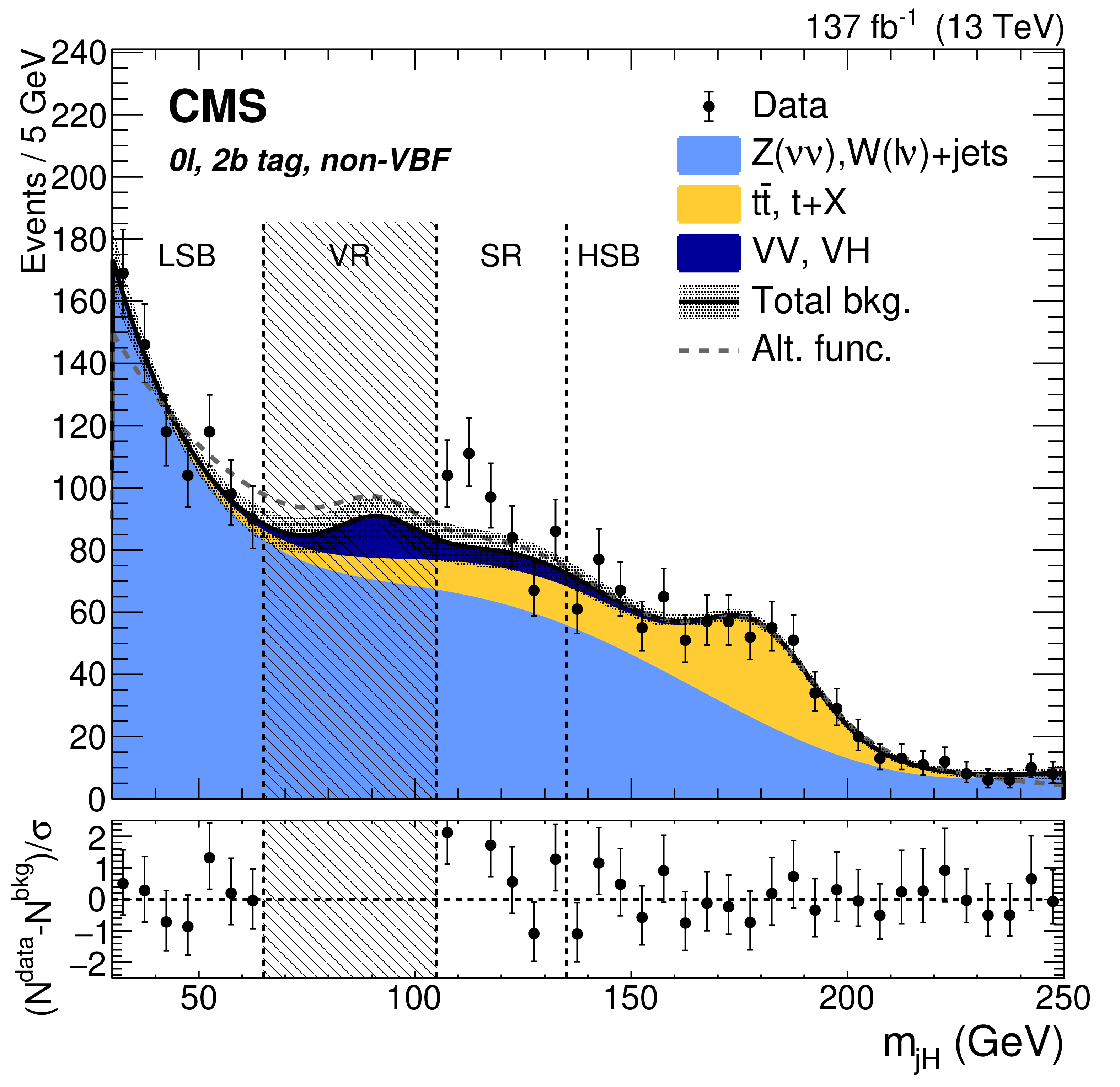
png pdf	Figure 16: Search for $ \mathrm{X}\to\mathrm{V}\mathrm{H}(\mathrm{b}\mathrm{b}) $: Distributions of (left) the jet soft drop mass of a boosted Higgs boson candidate, labeled $ m_{\text{j}\mathrm{H}} $, and (right) the mass or transverse mass of the X resonance candidate, labeled $ m_{\mathrm{X}} $ and $ m_{\mathrm{X}}^{\mathrm{T}} $, respectively, in the $ \mathrm{Z}(\ell\ell)\mathrm{H}(\mathrm{b}\mathrm{b}) $ (upper) and $ \mathrm{Z}(\nu\nu)\mathrm{H}(\mathrm{b}\mathrm{b}) $ channels (lower). The shaded area depicts a veto region excluded from the analysis to minimize the event overlap with dedicated searches in the VV decay channel. Figures from Ref. [110].
png pdf	Figure 16-a: Search for $ \mathrm{X}\to\mathrm{V}\mathrm{H}(\mathrm{b}\mathrm{b}) $: Distributions of (left) the jet soft drop mass of a boosted Higgs boson candidate, labeled $ m_{\text{j}\mathrm{H}} $, and (right) the mass or transverse mass of the X resonance candidate, labeled $ m_{\mathrm{X}} $ and $ m_{\mathrm{X}}^{\mathrm{T}} $, respectively, in the $ \mathrm{Z}(\ell\ell)\mathrm{H}(\mathrm{b}\mathrm{b}) $ (upper) and $ \mathrm{Z}(\nu\nu)\mathrm{H}(\mathrm{b}\mathrm{b}) $ channels (lower). The shaded area depicts a veto region excluded from the analysis to minimize the event overlap with dedicated searches in the VV decay channel. Figures from Ref. [110].
png pdf	Figure 16-b: Search for $ \mathrm{X}\to\mathrm{V}\mathrm{H}(\mathrm{b}\mathrm{b}) $: Distributions of (left) the jet soft drop mass of a boosted Higgs boson candidate, labeled $ m_{\text{j}\mathrm{H}} $, and (right) the mass or transverse mass of the X resonance candidate, labeled $ m_{\mathrm{X}} $ and $ m_{\mathrm{X}}^{\mathrm{T}} $, respectively, in the $ \mathrm{Z}(\ell\ell)\mathrm{H}(\mathrm{b}\mathrm{b}) $ (upper) and $ \mathrm{Z}(\nu\nu)\mathrm{H}(\mathrm{b}\mathrm{b}) $ channels (lower). The shaded area depicts a veto region excluded from the analysis to minimize the event overlap with dedicated searches in the VV decay channel. Figures from Ref. [110].
png pdf	Figure 16-c: Search for $ \mathrm{X}\to\mathrm{V}\mathrm{H}(\mathrm{b}\mathrm{b}) $: Distributions of (left) the jet soft drop mass of a boosted Higgs boson candidate, labeled $ m_{\text{j}\mathrm{H}} $, and (right) the mass or transverse mass of the X resonance candidate, labeled $ m_{\mathrm{X}} $ and $ m_{\mathrm{X}}^{\mathrm{T}} $, respectively, in the $ \mathrm{Z}(\ell\ell)\mathrm{H}(\mathrm{b}\mathrm{b}) $ (upper) and $ \mathrm{Z}(\nu\nu)\mathrm{H}(\mathrm{b}\mathrm{b}) $ channels (lower). The shaded area depicts a veto region excluded from the analysis to minimize the event overlap with dedicated searches in the VV decay channel. Figures from Ref. [110].
png pdf	Figure 16-d: Search for $ \mathrm{X}\to\mathrm{V}\mathrm{H}(\mathrm{b}\mathrm{b}) $: Distributions of (left) the jet soft drop mass of a boosted Higgs boson candidate, labeled $ m_{\text{j}\mathrm{H}} $, and (right) the mass or transverse mass of the X resonance candidate, labeled $ m_{\mathrm{X}} $ and $ m_{\mathrm{X}}^{\mathrm{T}} $, respectively, in the $ \mathrm{Z}(\ell\ell)\mathrm{H}(\mathrm{b}\mathrm{b}) $ (upper) and $ \mathrm{Z}(\nu\nu)\mathrm{H}(\mathrm{b}\mathrm{b}) $ channels (lower). The shaded area depicts a veto region excluded from the analysis to minimize the event overlap with dedicated searches in the VV decay channel. Figures from Ref. [110].
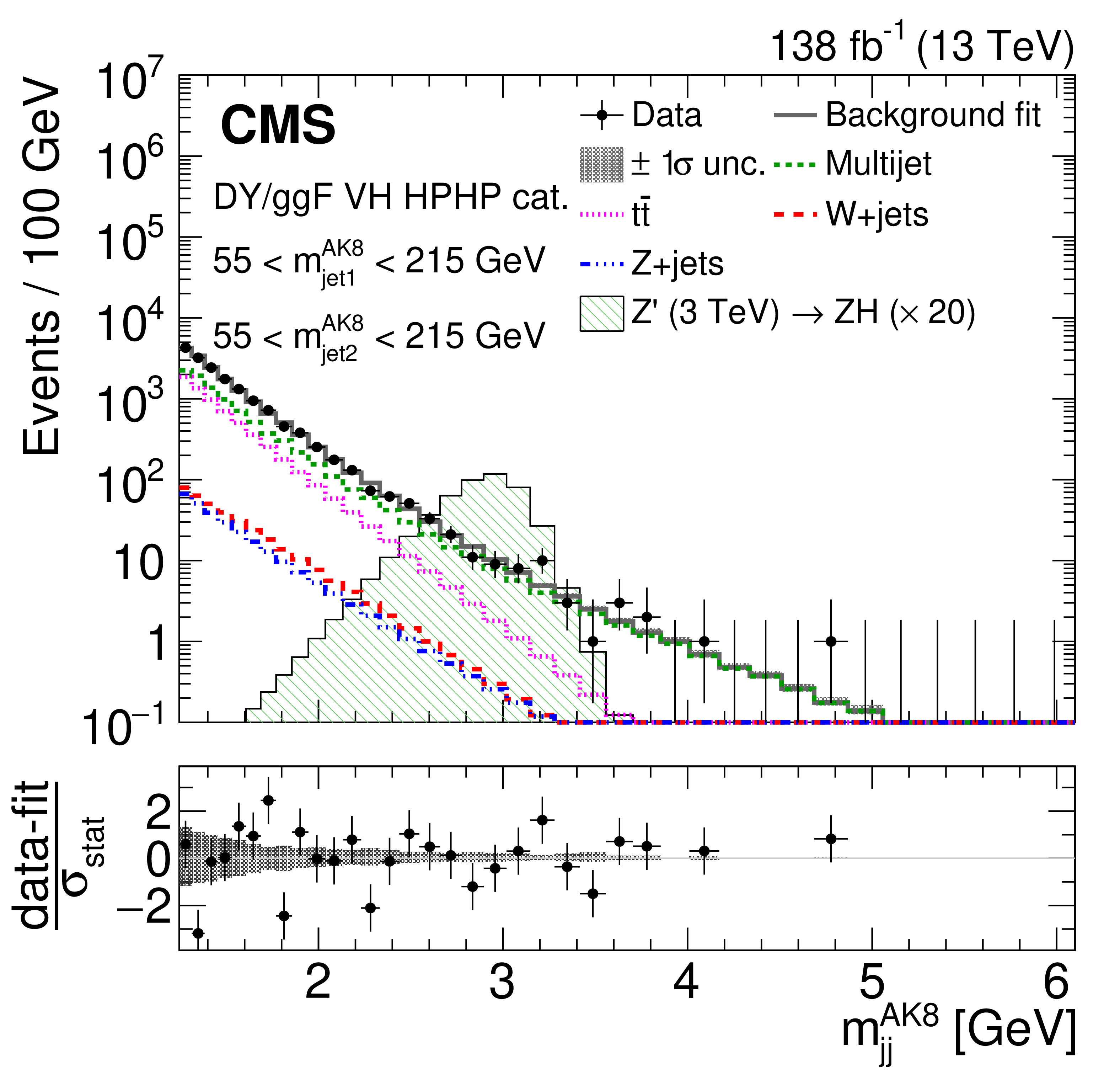
png pdf	Figure 17: Search for $ \mathrm{X}\to\mathrm{V} $ (qq) $ \mathrm{H}(\mathrm{b}\mathrm{b}) $: Distributions of (left) the soft drop mass $ m_{\mathrm{SD}} $ variable, labelled as $ m_{\text{jet1}}^{\text{AK8}} $, and (right) the dijet mass $ m_{\mathrm{jj}}^{\mathrm{AK8}} $ in the $ \mathrm{V}(\mathrm{q}\mathrm{q})\mathrm{H}(\mathrm{b}\mathrm{b}) $ channel [111]. The individual contributions of the background model are shown by open histograms with different colours and line styles. The signal of a Z' boson with a mass of 3 TeV decaying via $ \mathrm{Z}\to\text{qq} $ and $ \mathrm{H}\to\mathrm{b}\mathrm{b} $ is also shown, by a green filled histogram. Figure from Ref. [111].
png pdf	Figure 17-a: Search for $ \mathrm{X}\to\mathrm{V} $ (qq) $ \mathrm{H}(\mathrm{b}\mathrm{b}) $: Distributions of (left) the soft drop mass $ m_{\mathrm{SD}} $ variable, labelled as $ m_{\text{jet1}}^{\text{AK8}} $, and (right) the dijet mass $ m_{\mathrm{jj}}^{\mathrm{AK8}} $ in the $ \mathrm{V}(\mathrm{q}\mathrm{q})\mathrm{H}(\mathrm{b}\mathrm{b}) $ channel [111]. The individual contributions of the background model are shown by open histograms with different colours and line styles. The signal of a Z' boson with a mass of 3 TeV decaying via $ \mathrm{Z}\to\text{qq} $ and $ \mathrm{H}\to\mathrm{b}\mathrm{b} $ is also shown, by a green filled histogram. Figure from Ref. [111].
png pdf	Figure 17-b: Search for $ \mathrm{X}\to\mathrm{V} $ (qq) $ \mathrm{H}(\mathrm{b}\mathrm{b}) $: Distributions of (left) the soft drop mass $ m_{\mathrm{SD}} $ variable, labelled as $ m_{\text{jet1}}^{\text{AK8}} $, and (right) the dijet mass $ m_{\mathrm{jj}}^{\mathrm{AK8}} $ in the $ \mathrm{V}(\mathrm{q}\mathrm{q})\mathrm{H}(\mathrm{b}\mathrm{b}) $ channel [111]. The individual contributions of the background model are shown by open histograms with different colours and line styles. The signal of a Z' boson with a mass of 3 TeV decaying via $ \mathrm{Z}\to\text{qq} $ and $ \mathrm{H}\to\mathrm{b}\mathrm{b} $ is also shown, by a green filled histogram. Figure from Ref. [111].
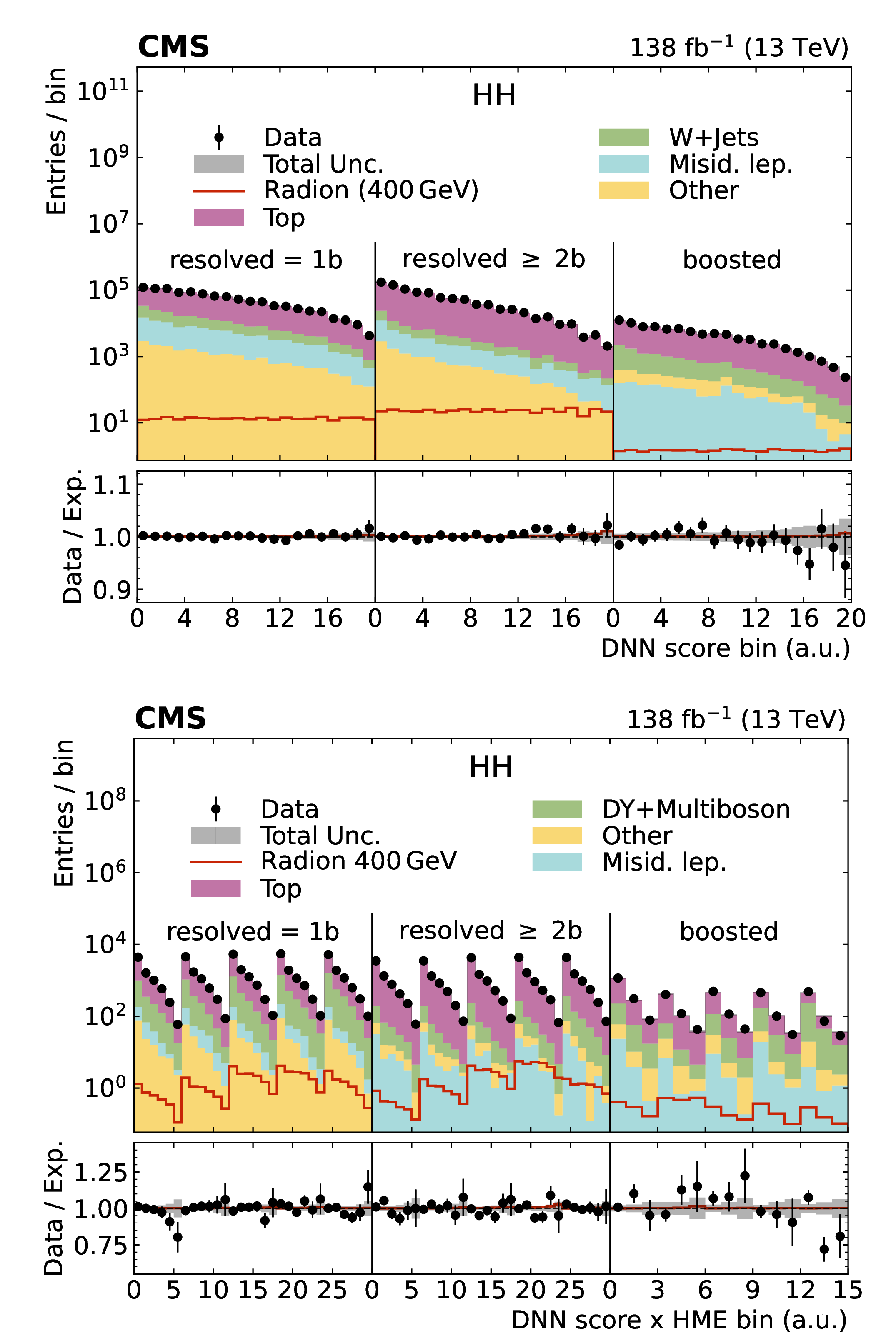
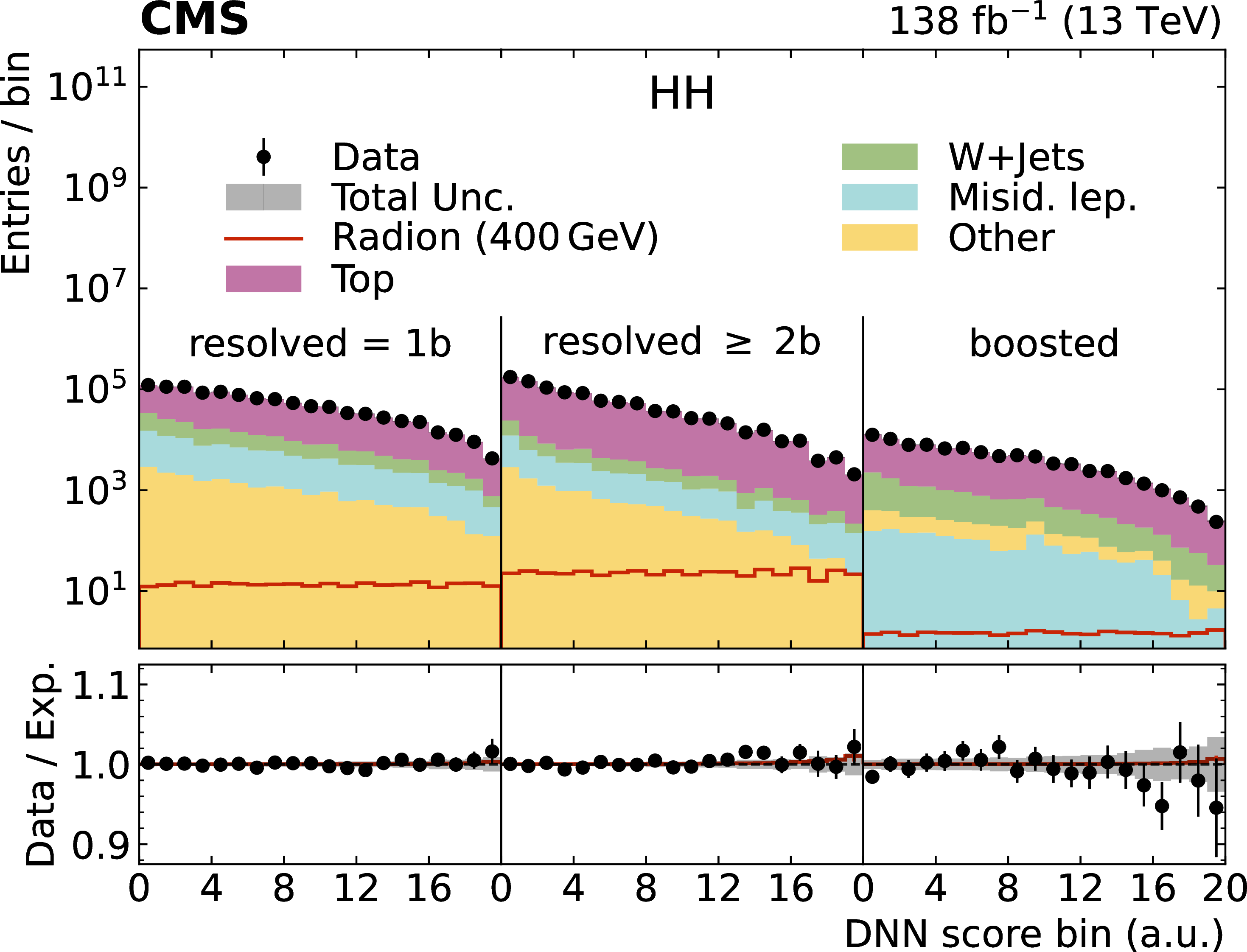
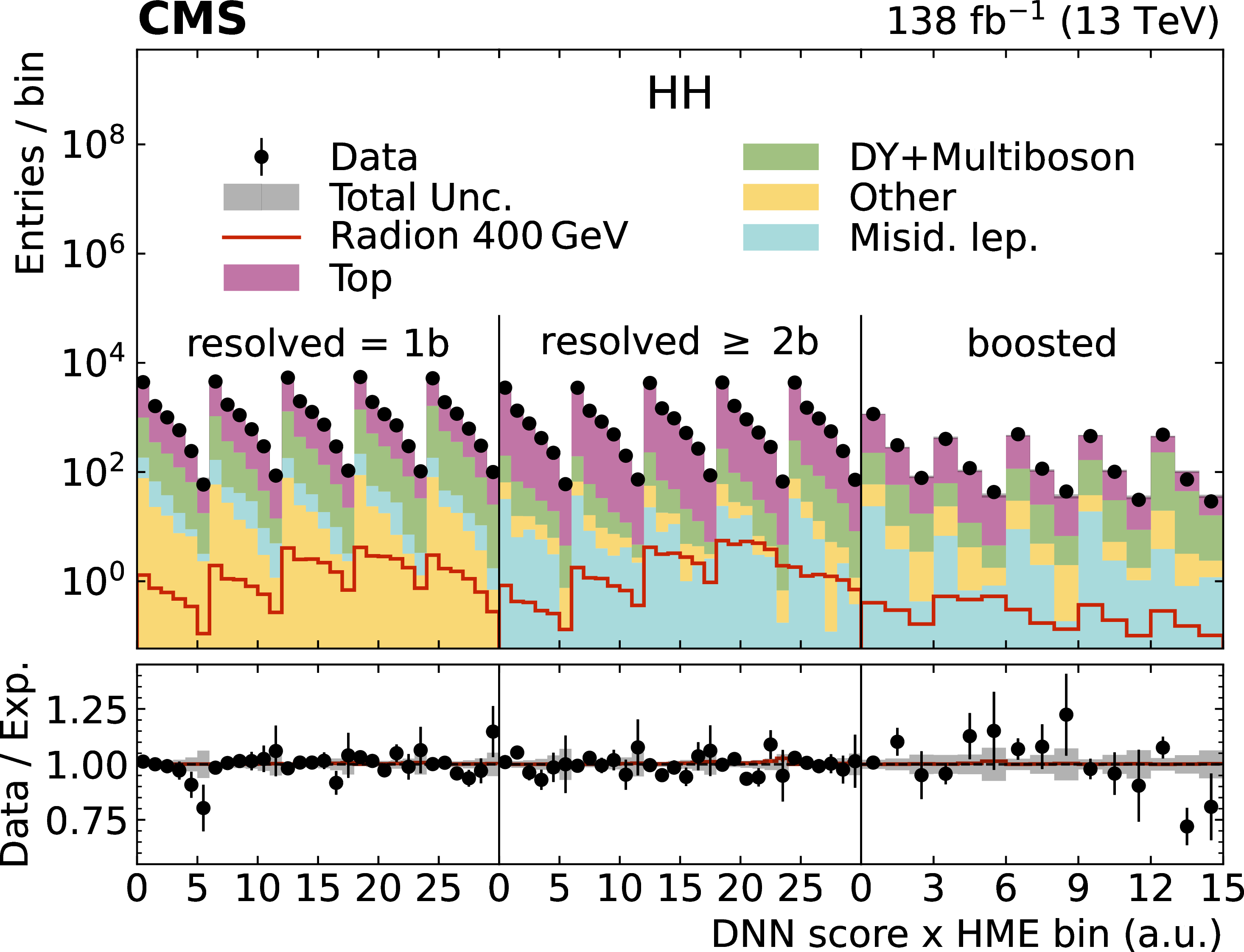
png pdf	Figure 18: Search for $ \mathrm{X}\to\mathrm{H}(\mathrm{b}\mathrm{b})\mathrm{H}(\mathrm{W}\mathrm{W}) $: Distributions of the DNN output for events in the signal nodes of the (upper) SL and (lower) DL categories of the $ \mathrm{H}(\mathrm{b}\mathrm{b})\mathrm{H}(\mathrm{W} \mathrm{W}) $ analysis based on merged and resolved jets [112]. The distributions for a signal of a resonant radion with a mass of 400 GeV is also shown, by an open red histogram. Figure from Ref. [112].
png pdf	Figure 18-a: Search for $ \mathrm{X}\to\mathrm{H}(\mathrm{b}\mathrm{b})\mathrm{H}(\mathrm{W}\mathrm{W}) $: Distributions of the DNN output for events in the signal nodes of the (upper) SL and (lower) DL categories of the $ \mathrm{H}(\mathrm{b}\mathrm{b})\mathrm{H}(\mathrm{W} \mathrm{W}) $ analysis based on merged and resolved jets [112]. The distributions for a signal of a resonant radion with a mass of 400 GeV is also shown, by an open red histogram. Figure from Ref. [112].
png pdf	Figure 18-b: Search for $ \mathrm{X}\to\mathrm{H}(\mathrm{b}\mathrm{b})\mathrm{H}(\mathrm{W}\mathrm{W}) $: Distributions of the DNN output for events in the signal nodes of the (upper) SL and (lower) DL categories of the $ \mathrm{H}(\mathrm{b}\mathrm{b})\mathrm{H}(\mathrm{W} \mathrm{W}) $ analysis based on merged and resolved jets [112]. The distributions for a signal of a resonant radion with a mass of 400 GeV is also shown, by an open red histogram. Figure from Ref. [112].
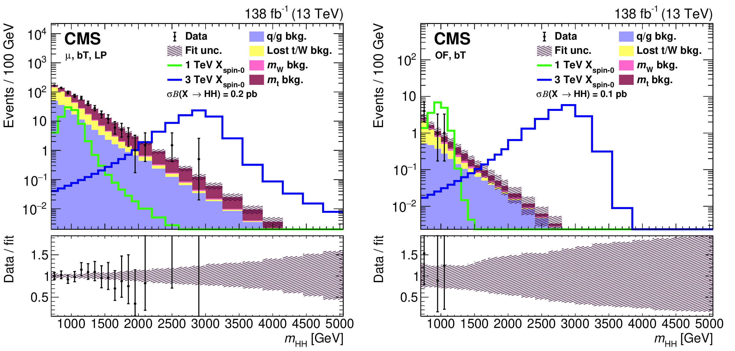
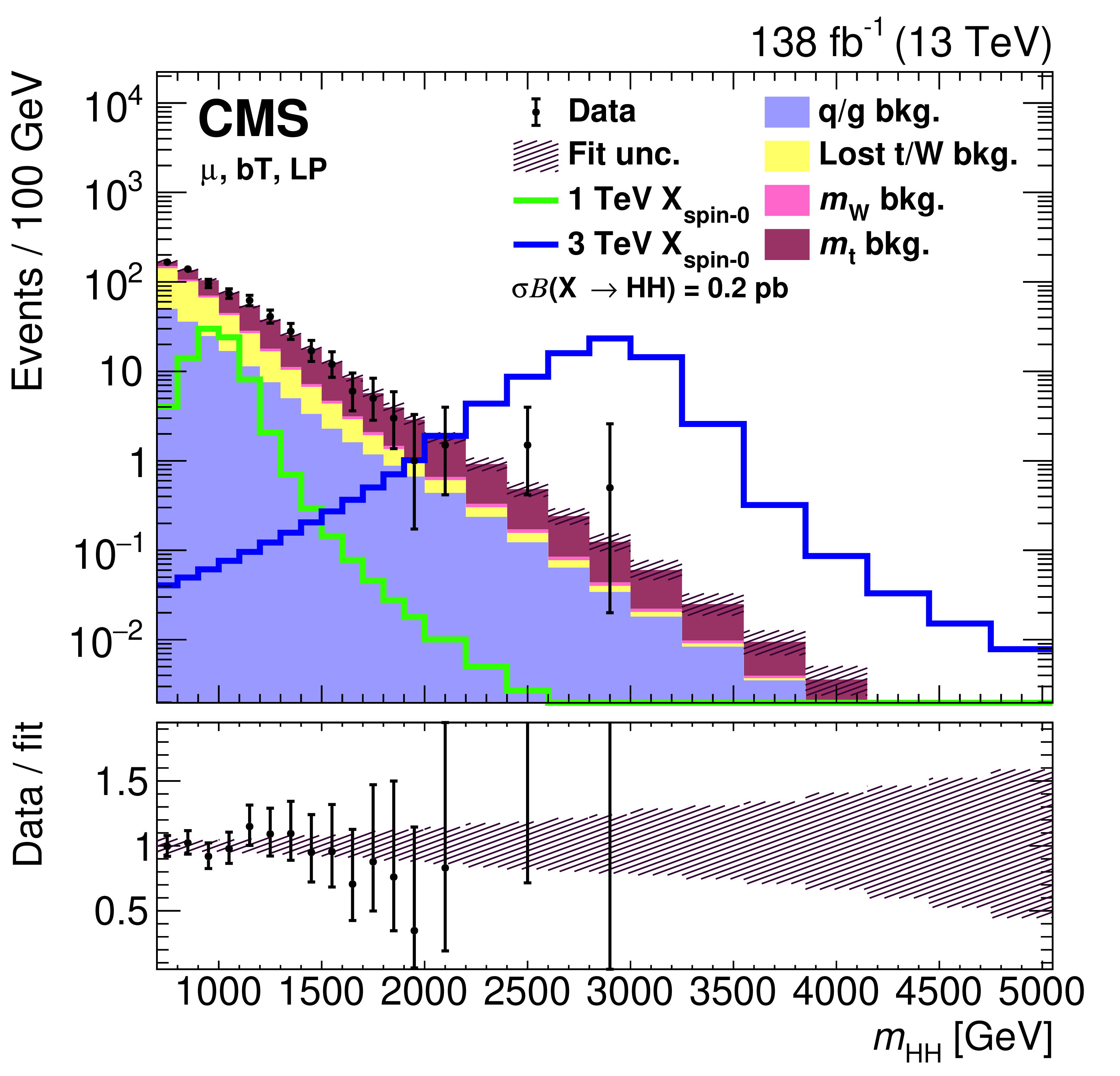
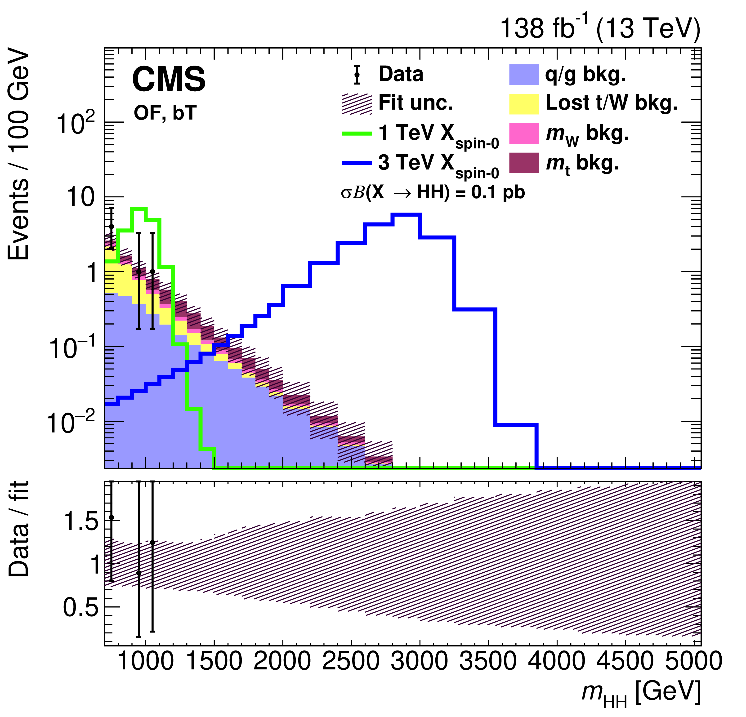
png pdf	Figure 19: Search for $ \mathrm{X}\to\mathrm{H}(\mathrm{b}\mathrm{b})\mathrm{H}(\mathrm{W}\mathrm{W}) $: Distributions of the $ m_{{\mathrm{H}\mathrm{H}}} $ variable, in the (left) SL and (right) DL categories of the $ \mathrm{H}(\mathrm{b}\mathrm{b})\mathrm{H}(\mathrm{W}\mathrm{W}) $ analysis with merged jets [113]. Expected signal distributions from a spin-0 resonance with a mass of 1 or 3 TeV are also shown, by the open green and blue histograms. Figure from Ref. [113].
png pdf	Figure 19-a: Search for $ \mathrm{X}\to\mathrm{H}(\mathrm{b}\mathrm{b})\mathrm{H}(\mathrm{W}\mathrm{W}) $: Distributions of the $ m_{{\mathrm{H}\mathrm{H}}} $ variable, in the (left) SL and (right) DL categories of the $ \mathrm{H}(\mathrm{b}\mathrm{b})\mathrm{H}(\mathrm{W}\mathrm{W}) $ analysis with merged jets [113]. Expected signal distributions from a spin-0 resonance with a mass of 1 or 3 TeV are also shown, by the open green and blue histograms. Figure from Ref. [113].
png pdf	Figure 19-b: Search for $ \mathrm{X}\to\mathrm{H}(\mathrm{b}\mathrm{b})\mathrm{H}(\mathrm{W}\mathrm{W}) $: Distributions of the $ m_{{\mathrm{H}\mathrm{H}}} $ variable, in the (left) SL and (right) DL categories of the $ \mathrm{H}(\mathrm{b}\mathrm{b})\mathrm{H}(\mathrm{W}\mathrm{W}) $ analysis with merged jets [113]. Expected signal distributions from a spin-0 resonance with a mass of 1 or 3 TeV are also shown, by the open green and blue histograms. Figure from Ref. [113].
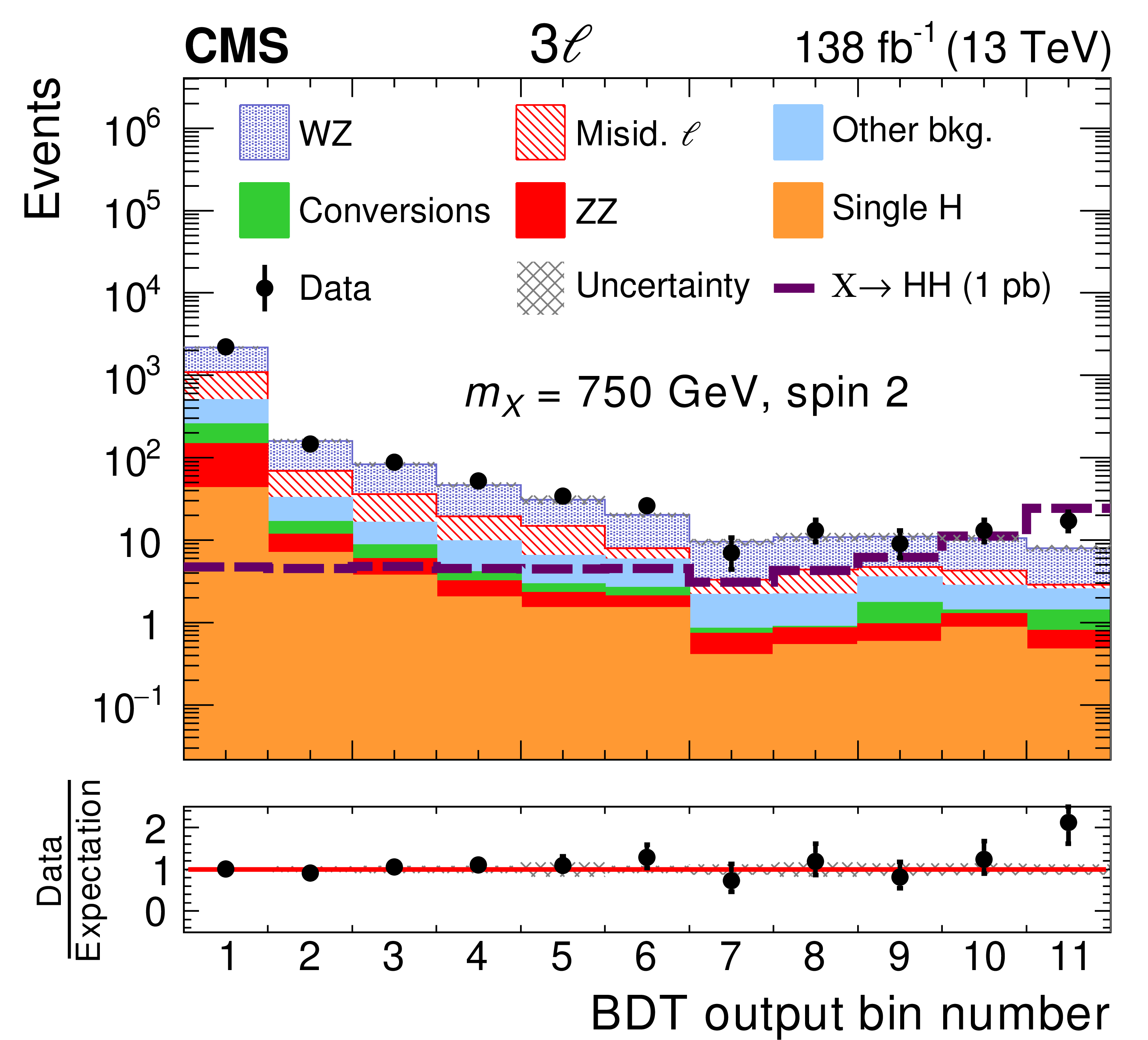
png pdf	Figure 20: Search for $ \mathrm{X}\to\mathrm{H}\mathrm{H} $ in multi-lepton final states: Distributions of the BDT classifier output for events in the (left) 2 $ \ell\text{ss} $ and (right) 3 $ \ell $ categories of the $ \mathrm{H}(\mathrm{W}\mathrm{W}+\tau\tau)\mathrm{H}(\mathrm{W}\mathrm{W}+\tau\tau) $ analysis in multilepton final states [114]. The expected signal for a spin-2 resonance with a mass of 750 GeV resonant HH signal is shown, by the open dashed histogram. The signal is normalized to a a cross section of 1\unitpb. The distributions of the estimated background processes and corresponding uncertainties are shown after a fit of the signal plus background hypothesis to the data. Figure from Ref. [114].
png pdf	Figure 20-a: Search for $ \mathrm{X}\to\mathrm{H}\mathrm{H} $ in multi-lepton final states: Distributions of the BDT classifier output for events in the (left) 2 $ \ell\text{ss} $ and (right) 3 $ \ell $ categories of the $ \mathrm{H}(\mathrm{W}\mathrm{W}+\tau\tau)\mathrm{H}(\mathrm{W}\mathrm{W}+\tau\tau) $ analysis in multilepton final states [114]. The expected signal for a spin-2 resonance with a mass of 750 GeV resonant HH signal is shown, by the open dashed histogram. The signal is normalized to a a cross section of 1\unitpb. The distributions of the estimated background processes and corresponding uncertainties are shown after a fit of the signal plus background hypothesis to the data. Figure from Ref. [114].
png pdf	Figure 20-b: Search for $ \mathrm{X}\to\mathrm{H}\mathrm{H} $ in multi-lepton final states: Distributions of the BDT classifier output for events in the (left) 2 $ \ell\text{ss} $ and (right) 3 $ \ell $ categories of the $ \mathrm{H}(\mathrm{W}\mathrm{W}+\tau\tau)\mathrm{H}(\mathrm{W}\mathrm{W}+\tau\tau) $ analysis in multilepton final states [114]. The expected signal for a spin-2 resonance with a mass of 750 GeV resonant HH signal is shown, by the open dashed histogram. The signal is normalized to a a cross section of 1\unitpb. The distributions of the estimated background processes and corresponding uncertainties are shown after a fit of the signal plus background hypothesis to the data. Figure from Ref. [114].
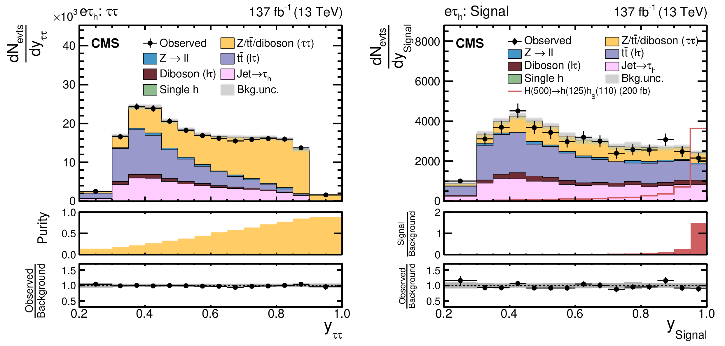
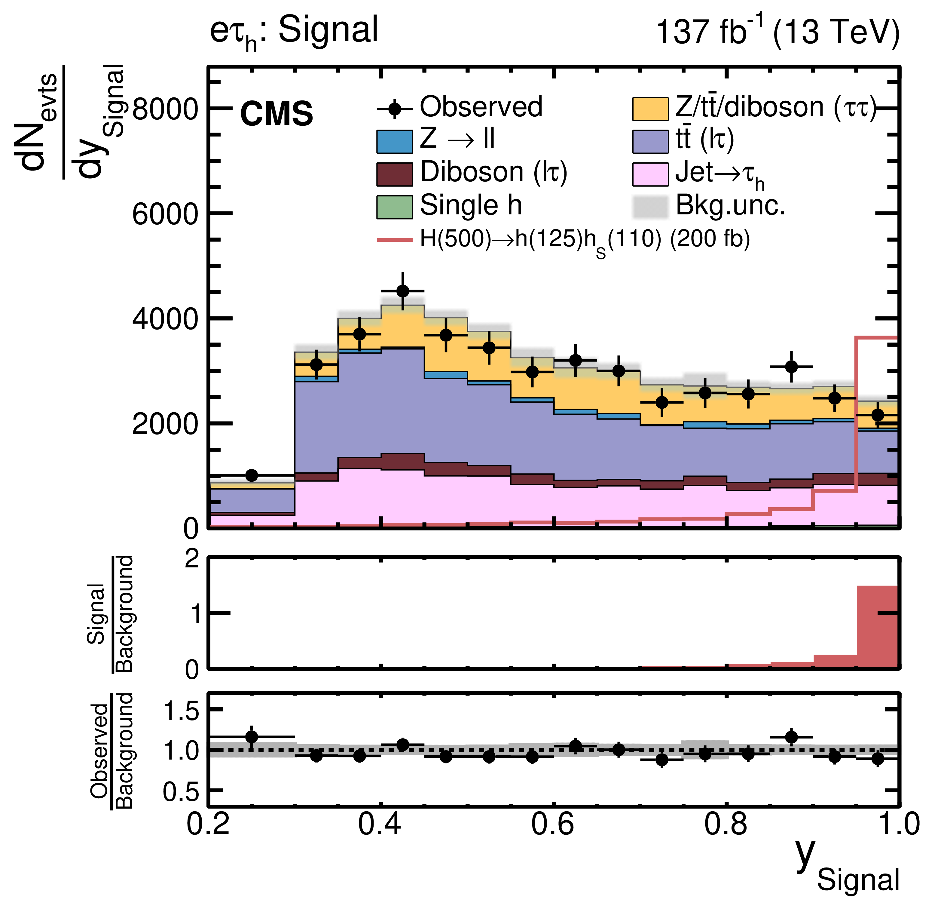
png pdf	Figure 21: Search for $ \mathrm{X}\to{\mathrm{Y}}(\mathrm{b}\mathrm{b})\mathrm{H}(\tau\tau) $: Distributions of the NN output scores $ y_{i} $, in different event categories after NN classification, based on a training for a resonance X with $ m_{\mathrm{X}}= $ 500 GeV and a resonance Y with 100 $ \leq m_{{\mathrm{Y}}} < $ 150 GeV in the $ \mathrm{e}\tau_\mathrm{h} $ final state of the $ \mathrm{H}(\tau\tau){\mathrm{Y}}(\mathrm{b}\mathrm{b}) $ analysis [115]. Shown are the (left) $ \tau\tau $ and (right) signal categories. For these figures, the data of all years have been combined. The uncertainty bands correspond to the combination of statistical and systematic uncertainties after the fit of the signal plus background hypothesis for $ m_{\mathrm{X}}= $ 500 GeV and $ m_{{\mathrm{Y}}}= $ 110 GeV to the data. In the lower panels of the figures the (left) purity and (right) fraction of the expected signal over background yields for a signal with a cross section of 200 fb, as well as the ratio of the obtained yields in data over the expectation based on only the background model, are shown. Figure from Ref. [115].
png pdf	Figure 21-a: Search for $ \mathrm{X}\to{\mathrm{Y}}(\mathrm{b}\mathrm{b})\mathrm{H}(\tau\tau) $: Distributions of the NN output scores $ y_{i} $, in different event categories after NN classification, based on a training for a resonance X with $ m_{\mathrm{X}}= $ 500 GeV and a resonance Y with 100 $ \leq m_{{\mathrm{Y}}} < $ 150 GeV in the $ \mathrm{e}\tau_\mathrm{h} $ final state of the $ \mathrm{H}(\tau\tau){\mathrm{Y}}(\mathrm{b}\mathrm{b}) $ analysis [115]. Shown are the (left) $ \tau\tau $ and (right) signal categories. For these figures, the data of all years have been combined. The uncertainty bands correspond to the combination of statistical and systematic uncertainties after the fit of the signal plus background hypothesis for $ m_{\mathrm{X}}= $ 500 GeV and $ m_{{\mathrm{Y}}}= $ 110 GeV to the data. In the lower panels of the figures the (left) purity and (right) fraction of the expected signal over background yields for a signal with a cross section of 200 fb, as well as the ratio of the obtained yields in data over the expectation based on only the background model, are shown. Figure from Ref. [115].
png pdf	Figure 21-b: Search for $ \mathrm{X}\to{\mathrm{Y}}(\mathrm{b}\mathrm{b})\mathrm{H}(\tau\tau) $: Distributions of the NN output scores $ y_{i} $, in different event categories after NN classification, based on a training for a resonance X with $ m_{\mathrm{X}}= $ 500 GeV and a resonance Y with 100 $ \leq m_{{\mathrm{Y}}} < $ 150 GeV in the $ \mathrm{e}\tau_\mathrm{h} $ final state of the $ \mathrm{H}(\tau\tau){\mathrm{Y}}(\mathrm{b}\mathrm{b}) $ analysis [115]. Shown are the (left) $ \tau\tau $ and (right) signal categories. For these figures, the data of all years have been combined. The uncertainty bands correspond to the combination of statistical and systematic uncertainties after the fit of the signal plus background hypothesis for $ m_{\mathrm{X}}= $ 500 GeV and $ m_{{\mathrm{Y}}}= $ 110 GeV to the data. In the lower panels of the figures the (left) purity and (right) fraction of the expected signal over background yields for a signal with a cross section of 200 fb, as well as the ratio of the obtained yields in data over the expectation based on only the background model, are shown. Figure from Ref. [115].
png pdf	Figure 22: Search for $ \mathrm{X}\to{\mathrm{Y}} $ (bb) $ \mathrm{H}(\gamma\gamma) $: Marginal distributions of the (left) $ m_{\gamma\gamma} $ and (right) $ m_{\mathrm{jj}} $ variables, in the high-purity SR (labeled ``CAT 0'') of the $ {\mathrm{Y}}(\mathrm{b}\mathrm{b})\mathrm{H}(\gamma\gamma) $ analysis [116]. The figure is shown, for a hypothesis of $ m_{\mathrm{X}}= $ 650 GeV and $ m_{{\mathrm{Y}}}= $ 90 GeV, for which the largest excess of events over the background model is observed. In the lower panels, the numbers of background-subtracted events are shown after the fit of the background model to the data. Figure from Ref. [116].
png pdf	Figure 22-a: Search for $ \mathrm{X}\to{\mathrm{Y}} $ (bb) $ \mathrm{H}(\gamma\gamma) $: Marginal distributions of the (left) $ m_{\gamma\gamma} $ and (right) $ m_{\mathrm{jj}} $ variables, in the high-purity SR (labeled ``CAT 0'') of the $ {\mathrm{Y}}(\mathrm{b}\mathrm{b})\mathrm{H}(\gamma\gamma) $ analysis [116]. The figure is shown, for a hypothesis of $ m_{\mathrm{X}}= $ 650 GeV and $ m_{{\mathrm{Y}}}= $ 90 GeV, for which the largest excess of events over the background model is observed. In the lower panels, the numbers of background-subtracted events are shown after the fit of the background model to the data. Figure from Ref. [116].
png pdf	Figure 22-b: Search for $ \mathrm{X}\to{\mathrm{Y}} $ (bb) $ \mathrm{H}(\gamma\gamma) $: Marginal distributions of the (left) $ m_{\gamma\gamma} $ and (right) $ m_{\mathrm{jj}} $ variables, in the high-purity SR (labeled ``CAT 0'') of the $ {\mathrm{Y}}(\mathrm{b}\mathrm{b})\mathrm{H}(\gamma\gamma) $ analysis [116]. The figure is shown, for a hypothesis of $ m_{\mathrm{X}}= $ 650 GeV and $ m_{{\mathrm{Y}}}= $ 90 GeV, for which the largest excess of events over the background model is observed. In the lower panels, the numbers of background-subtracted events are shown after the fit of the background model to the data. Figure from Ref. [116].
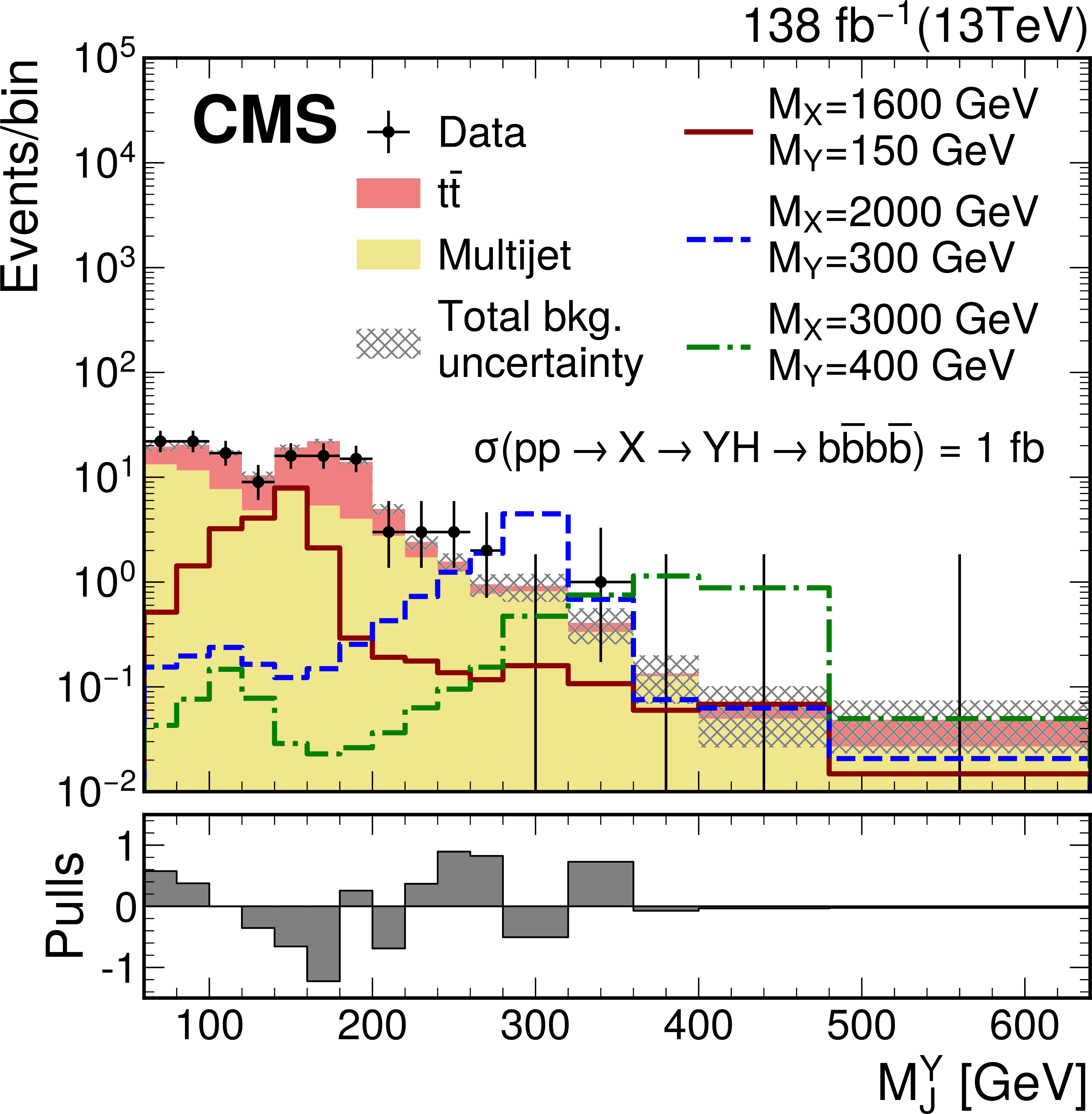
png pdf	Figure 23: Search for $ \mathrm{X}\to{\mathrm{Y}}(\mathrm{b}\mathrm{b})\mathrm{H}(\mathrm{b}\mathrm{b}) $: Distributions of the (left) soft-drop mass of the boosted Y candidate, labeled $ M^{\mathrm{Y}}_\text{J} $, and (right) the dijet mass of the Y and H candidates, $ M_\text{JJ} $, in the high-purity SR of the $ {\mathrm{Y}}(\mathrm{b}\mathrm{b})\mathrm{H}(\mathrm{b}\mathrm{b}) $ analysis with two merged $ \mathrm{b}\mathrm{b} $ jets [117]. The distributions as expected for signals with three different values of $ m_{\mathrm{X}} $ and $ m_{{\mathrm{Y}}} $ (labeled $ M^\mathrm{X} $ and $ M^{\mathrm{Y}} $) are also shown. In the lower panels the statistical pull in each bin is displayed. Figure from Ref. [117].
png pdf	Figure 23-a: Search for $ \mathrm{X}\to{\mathrm{Y}}(\mathrm{b}\mathrm{b})\mathrm{H}(\mathrm{b}\mathrm{b}) $: Distributions of the (left) soft-drop mass of the boosted Y candidate, labeled $ M^{\mathrm{Y}}_\text{J} $, and (right) the dijet mass of the Y and H candidates, $ M_\text{JJ} $, in the high-purity SR of the $ {\mathrm{Y}}(\mathrm{b}\mathrm{b})\mathrm{H}(\mathrm{b}\mathrm{b}) $ analysis with two merged $ \mathrm{b}\mathrm{b} $ jets [117]. The distributions as expected for signals with three different values of $ m_{\mathrm{X}} $ and $ m_{{\mathrm{Y}}} $ (labeled $ M^\mathrm{X} $ and $ M^{\mathrm{Y}} $) are also shown. In the lower panels the statistical pull in each bin is displayed. Figure from Ref. [117].
png pdf	Figure 23-b: Search for $ \mathrm{X}\to{\mathrm{Y}}(\mathrm{b}\mathrm{b})\mathrm{H}(\mathrm{b}\mathrm{b}) $: Distributions of the (left) soft-drop mass of the boosted Y candidate, labeled $ M^{\mathrm{Y}}_\text{J} $, and (right) the dijet mass of the Y and H candidates, $ M_\text{JJ} $, in the high-purity SR of the $ {\mathrm{Y}}(\mathrm{b}\mathrm{b})\mathrm{H}(\mathrm{b}\mathrm{b}) $ analysis with two merged $ \mathrm{b}\mathrm{b} $ jets [117]. The distributions as expected for signals with three different values of $ m_{\mathrm{X}} $ and $ m_{{\mathrm{Y}}} $ (labeled $ M^\mathrm{X} $ and $ M^{\mathrm{Y}} $) are also shown. In the lower panels the statistical pull in each bin is displayed. Figure from Ref. [117].
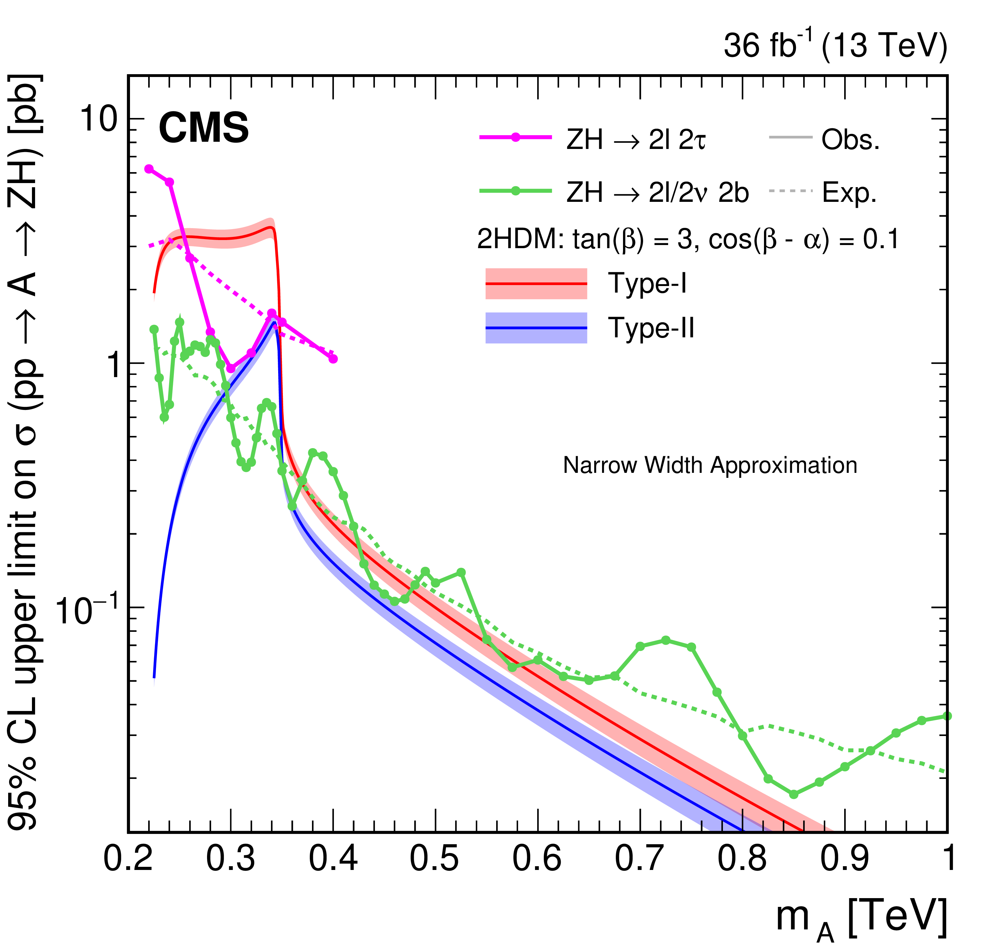
png pdf	Figure 24: Search for $ \mathrm{X}\to\mathrm{Z}\mathrm{H} $: Observed and expected 95% CL upper limits on the product of the cross section $ \sigma $ for the production of an $ {\mathrm{A}} $ boson, via gluon-gluon fusion and the branching fraction $ \mathcal{B} $ for the $ {\mathrm{A}}\to\mathrm{Z}\mathrm{H} $ decay. The limits are given in \unitpb as functions of $ m_{{\mathrm{A}}} $. The markers connected with solid lines (dashed lines) indicate the observed (expected) limits. The green (magenta) lines refer to the $ \mathrm{Z}(\ell\ell+\nu\nu)\mathrm{H}(\mathrm{b}\mathrm{b}) $ [108] ($ \mathrm{Z}(\ell\ell)\mathrm{H}(\tau\tau ) $ [107]) analysis. The red and blue solid lines indicate the product $ \sigma\mathcal{B} $ as expected by the 2HDM Type I and Type II models, respectively, for the parameters $ \tan\beta= $ 3 and $ \cos(\beta-\alpha)= $ 0.1. The shaded areas associated with these predictions indicate the corresponding model uncertainties. The results and model predictions have been adapted from Refs. [108,107].
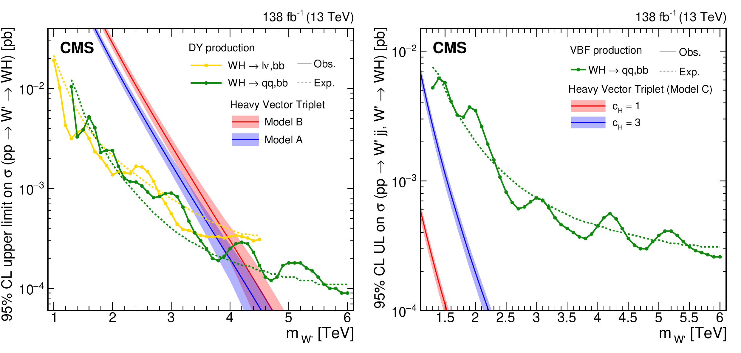
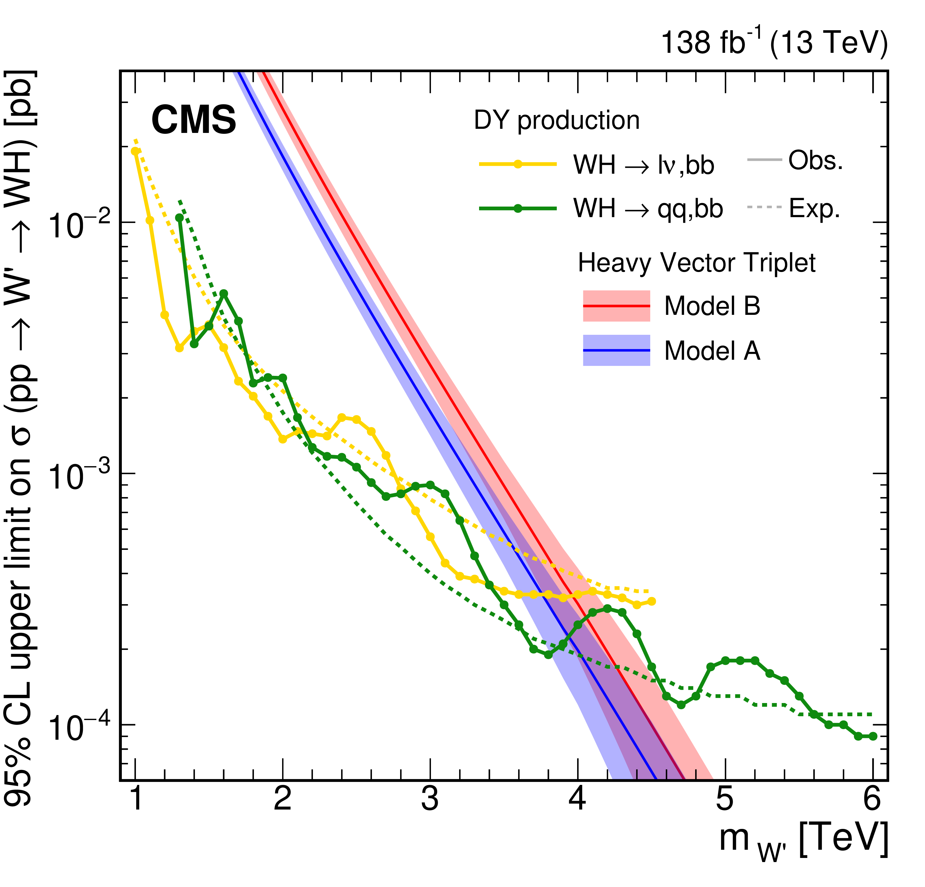
png pdf	Figure 25: Search for $ \mathrm{X}\to\mathrm{W}\mathrm{H} $: Observed and expected 95% CL upper limits on the product of the cross section $ \sigma $ for the production of a W' spin-1 resonance, via (left) DY production or (right) vector boson fusion and the branching fraction $ \mathcal{B} $ for the $ \mathrm{W^{'}}\to\mathrm{W}\mathrm{H} $ decay. The solid lines represent the observed and the dotted lines the expected limits. The theory predictions from the heavy vector triplet models A, B, and C are also shown.
png pdf	Figure 25-a: Search for $ \mathrm{X}\to\mathrm{W}\mathrm{H} $: Observed and expected 95% CL upper limits on the product of the cross section $ \sigma $ for the production of a W' spin-1 resonance, via (left) DY production or (right) vector boson fusion and the branching fraction $ \mathcal{B} $ for the $ \mathrm{W^{'}}\to\mathrm{W}\mathrm{H} $ decay. The solid lines represent the observed and the dotted lines the expected limits. The theory predictions from the heavy vector triplet models A, B, and C are also shown.
png pdf	Figure 25-b: Search for $ \mathrm{X}\to\mathrm{W}\mathrm{H} $: Observed and expected 95% CL upper limits on the product of the cross section $ \sigma $ for the production of a W' spin-1 resonance, via (left) DY production or (right) vector boson fusion and the branching fraction $ \mathcal{B} $ for the $ \mathrm{W^{'}}\to\mathrm{W}\mathrm{H} $ decay. The solid lines represent the observed and the dotted lines the expected limits. The theory predictions from the heavy vector triplet models A, B, and C are also shown.
png pdf	Figure 26: Search for $ \mathrm{X}\to\mathrm{Z}\mathrm{H} $: Observed and expected 95% CL upper limits on the product of the cross section $ \sigma $ for the production of a Z' spin-1 resonance, via (left) DY production or (right) vector boson fusion and the branching fraction $ \mathcal{B} $ for the $ \mathrm{Z}^{'}\to\mathrm{Z}\mathrm{H} $ decay. The solid lines represent the observed and the dotted lines the expected limits. The theory predictions from the heavy vector triplet models A, B and C are also shown.
png pdf	Figure 26-a: Search for $ \mathrm{X}\to\mathrm{Z}\mathrm{H} $: Observed and expected 95% CL upper limits on the product of the cross section $ \sigma $ for the production of a Z' spin-1 resonance, via (left) DY production or (right) vector boson fusion and the branching fraction $ \mathcal{B} $ for the $ \mathrm{Z}^{'}\to\mathrm{Z}\mathrm{H} $ decay. The solid lines represent the observed and the dotted lines the expected limits. The theory predictions from the heavy vector triplet models A, B and C are also shown.
png pdf	Figure 26-b: Search for $ \mathrm{X}\to\mathrm{Z}\mathrm{H} $: Observed and expected 95% CL upper limits on the product of the cross section $ \sigma $ for the production of a Z' spin-1 resonance, via (left) DY production or (right) vector boson fusion and the branching fraction $ \mathcal{B} $ for the $ \mathrm{Z}^{'}\to\mathrm{Z}\mathrm{H} $ decay. The solid lines represent the observed and the dotted lines the expected limits. The theory predictions from the heavy vector triplet models A, B and C are also shown.
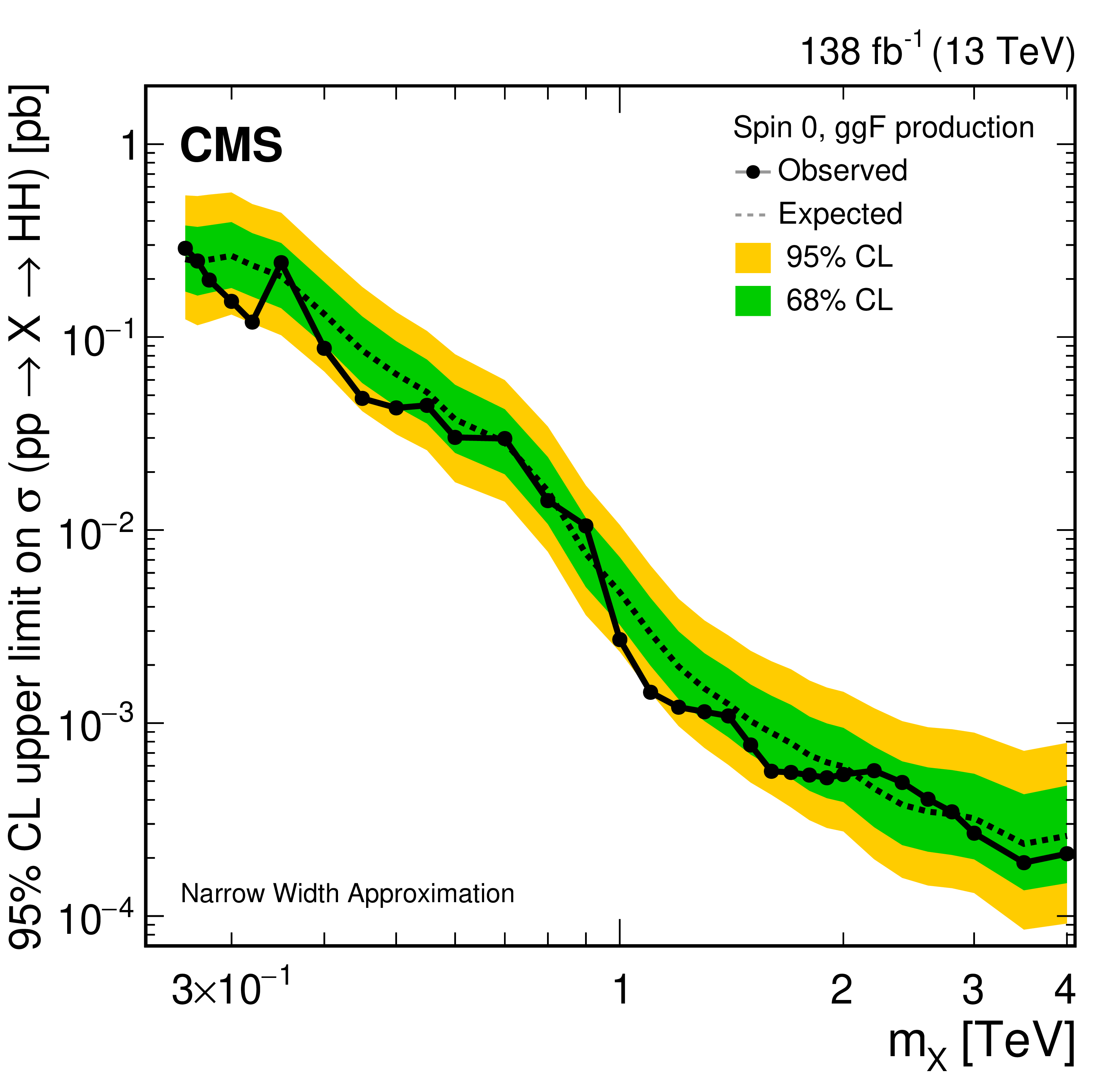
png pdf	Figure 27: Search for $ \mathrm{X}\to\mathrm{H}\mathrm{H} $/$ {\mathrm{G}} \to\mathrm{H}\mathrm{H} $: Observed and expected 95% CL upper limits on the product of the cross section $ \sigma $ for the production of a (left) spin-0 resonance X and (right) a spin-2 resonance G, via gluon-gluon fusion and the branching fraction $ \mathcal{B} $ for the corresponding HH decay. The results of the individual analyses presented in this report and the result of their combined likelihood analysis are shown. The observed limits are indicated by markers connected with solid lines and the expected limits by dashed lines.
png pdf	Figure 27-a: Search for $ \mathrm{X}\to\mathrm{H}\mathrm{H} $/$ {\mathrm{G}} \to\mathrm{H}\mathrm{H} $: Observed and expected 95% CL upper limits on the product of the cross section $ \sigma $ for the production of a (left) spin-0 resonance X and (right) a spin-2 resonance G, via gluon-gluon fusion and the branching fraction $ \mathcal{B} $ for the corresponding HH decay. The results of the individual analyses presented in this report and the result of their combined likelihood analysis are shown. The observed limits are indicated by markers connected with solid lines and the expected limits by dashed lines.
png pdf	Figure 27-b: Search for $ \mathrm{X}\to\mathrm{H}\mathrm{H} $/$ {\mathrm{G}} \to\mathrm{H}\mathrm{H} $: Observed and expected 95% CL upper limits on the product of the cross section $ \sigma $ for the production of a (left) spin-0 resonance X and (right) a spin-2 resonance G, via gluon-gluon fusion and the branching fraction $ \mathcal{B} $ for the corresponding HH decay. The results of the individual analyses presented in this report and the result of their combined likelihood analysis are shown. The observed limits are indicated by markers connected with solid lines and the expected limits by dashed lines.
png pdf	Figure 28: Search for $ \mathrm{X}\to\mathrm{H}\mathrm{H} $/$ {\mathrm{G}} \to\mathrm{H}\mathrm{H} $: Observed and expected 95% CL upper limits on the product of the cross section $ \sigma $ for the production of a (left) spin-0 resonance X and (right) a spin-2 resonance G, via gluon-gluon fusion, and the branching fraction $ \mathcal{B} $ for the corresponding HH decay, as obtained from the combined likelihood analysis of all contributing individual analyses presented in this report and shown in Fig. 27. In addition to the limit from the combined likelihood analysis the 68 and 95% central intervals for the expected upper limits in the absence of a signal are shown as coloured bands.
png pdf	Figure 28-a: Search for $ \mathrm{X}\to\mathrm{H}\mathrm{H} $/$ {\mathrm{G}} \to\mathrm{H}\mathrm{H} $: Observed and expected 95% CL upper limits on the product of the cross section $ \sigma $ for the production of a (left) spin-0 resonance X and (right) a spin-2 resonance G, via gluon-gluon fusion, and the branching fraction $ \mathcal{B} $ for the corresponding HH decay, as obtained from the combined likelihood analysis of all contributing individual analyses presented in this report and shown in Fig. 27. In addition to the limit from the combined likelihood analysis the 68 and 95% central intervals for the expected upper limits in the absence of a signal are shown as coloured bands.
png pdf	Figure 28-b: Search for $ \mathrm{X}\to\mathrm{H}\mathrm{H} $/$ {\mathrm{G}} \to\mathrm{H}\mathrm{H} $: Observed and expected 95% CL upper limits on the product of the cross section $ \sigma $ for the production of a (left) spin-0 resonance X and (right) a spin-2 resonance G, via gluon-gluon fusion, and the branching fraction $ \mathcal{B} $ for the corresponding HH decay, as obtained from the combined likelihood analysis of all contributing individual analyses presented in this report and shown in Fig. 27. In addition to the limit from the combined likelihood analysis the 68 and 95% central intervals for the expected upper limits in the absence of a signal are shown as coloured bands.
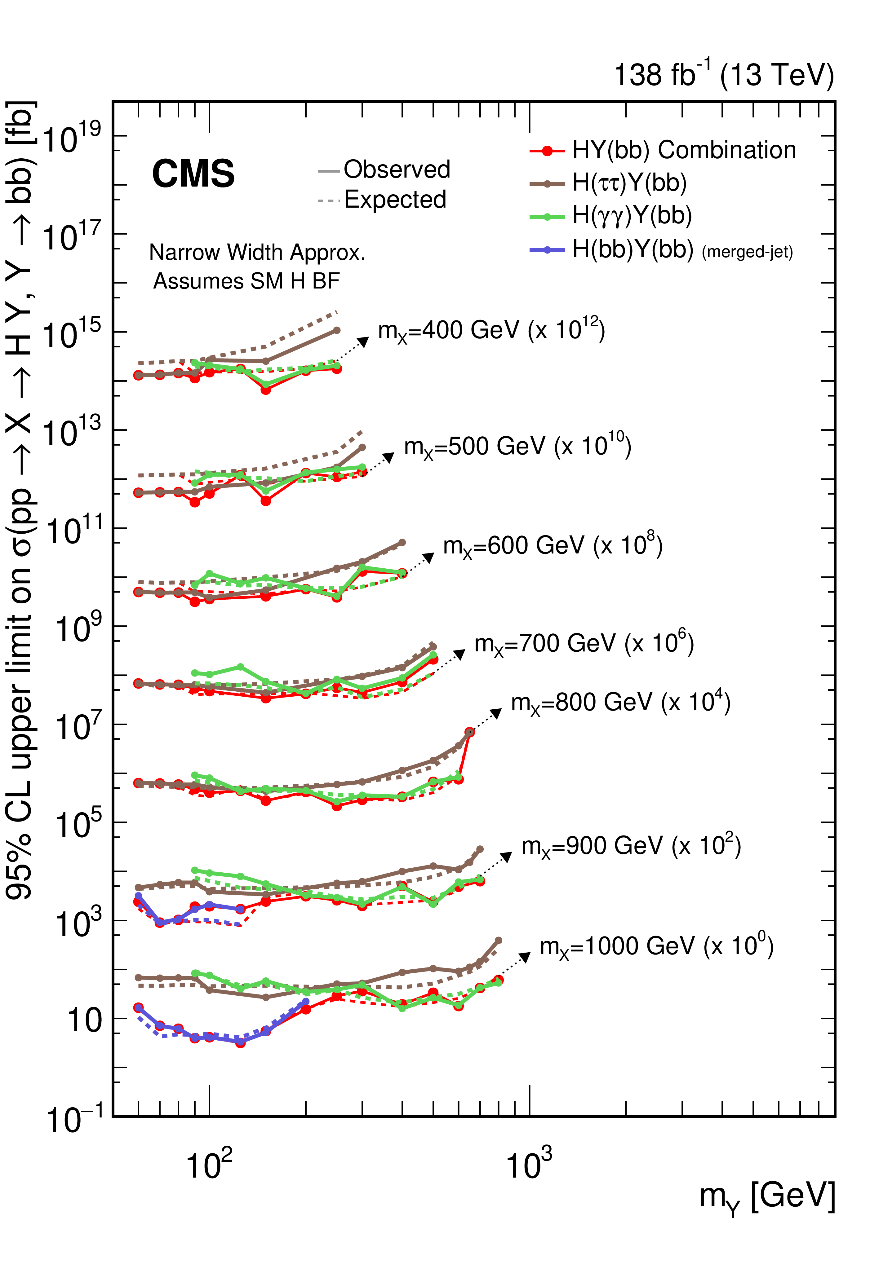
png pdf	Figure 29: Search for $ \mathrm{X}\to{\mathrm{Y}}\mathrm{H} $: Observed and expected upper limits, at 95% CL, on the product of the cross section $ \sigma $ for the production of a resonance X via gluon-gluon fusion and the branching fraction $ \mathcal{B} $ for the $ \mathrm{X}\to{\mathrm{Y}}(\mathrm{b}\mathrm{b}) \mathrm{H} $ decay. For the branching fractions of the $ \mathrm{H}\to\tau\tau $, $ \mathrm{H}\to\gamma\gamma $ and $ \mathrm{H}\to\mathrm{b}\mathrm{b} $ decays, the SM values are assumed. The results derived from the individual analyses presented in this report and the result of their combined likelihood analysis are shown as functions of $ m_{{\mathrm{Y}}} $ and $ m_{\mathrm{X}} $ for $ m_{\mathrm{X}}\le $ 1 TeV. Observed limits are indicated by markers connected with solid lines, expected limits by dashed lines. For presentation purposes, the limits have been scaled in successive steps by two orders of magnitude, each. For each set of graphs, a black arrow points to the $ m_{\mathrm{X}} $ related legend.
png pdf	Figure 30: Search for $ \mathrm{X}\to{\mathrm{Y}}\mathrm{H} $: Observed and expected upper limits, at 95% CL, on the product of the cross section $ \sigma $ for the production of a resonance X via gluon-gluon fusion and the branching fraction $ \mathcal{B} $ for the $ \mathrm{X}\to{\mathrm{Y}}(\mathrm{b}\mathrm{b}) \mathrm{H} $ decay. For the branching fractions of the $ \mathrm{H}\to\tau\tau $ and $ \mathrm{H}\to\mathrm{b}\mathrm{b} $ decays, the SM values are assumed. The results derived from the individual analyses presented in this report and the result of their combined likelihood analysis are shown as functions of $ m_{{\mathrm{Y}}} $ and $ m_{\mathrm{X}} $ for $ m_{\mathrm{X}}\ge $ 1.2 TeV. Observed limits are indicated by markers connected with solid lines, expected limits by dashed lines. For presentation purposes, the limits have been scaled in successive steps by four orders of magnitude, each. For each set of graphs, a black arrow points to the $ m_{\mathrm{X}} $ related legend.
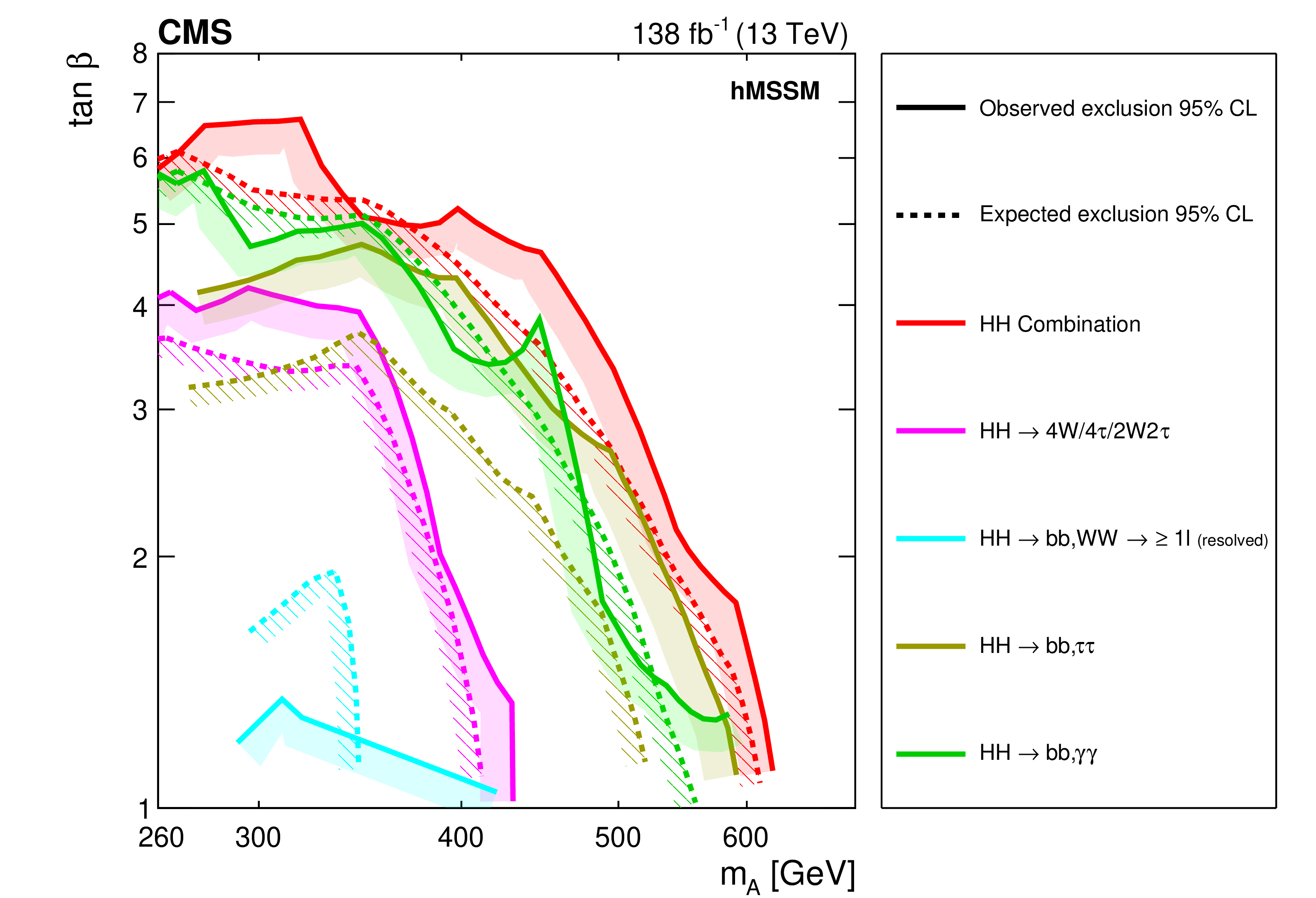
png pdf	Figure 31: Interpretation of the results from the searches for the $ \mathrm{X}\to{\mathrm{H}\mathrm{H}} $ decay, in the hMSSM model. In the upper part of the figure, the observed and expected exclusion contours at 95% CL, in the ($ m_{{\mathrm{A}}} $, $ \tan\beta $) plane, from the individual HH analyses presented in this report and their combined likelihood analysis are shown. In the lower part of the figure, a comparison of the region excluded by the combined likelihood analysis shown in the upper part of the figure with selected results from other searches for the production of heavy scalar bosons in the hMSSM, in $ \tau\tau $ [64], $ \mathrm{t} \overline{\mathrm{t}} $ [169] and WW [170] decays is shown. Also shown, are the results from one representative search for $ {\mathrm{A}}\to\mathrm{Z}\mathrm{H} $ [107] and indirect constraints obtained from measurements of the coupling strength of the observed H boson [47]. Results not marked by a club symbol are based on an integrated luminosity of 35.9 fb$^{-1}$.
png pdf	Figure 31-a: Interpretation of the results from the searches for the $ \mathrm{X}\to{\mathrm{H}\mathrm{H}} $ decay, in the hMSSM model. In the upper part of the figure, the observed and expected exclusion contours at 95% CL, in the ($ m_{{\mathrm{A}}} $, $ \tan\beta $) plane, from the individual HH analyses presented in this report and their combined likelihood analysis are shown. In the lower part of the figure, a comparison of the region excluded by the combined likelihood analysis shown in the upper part of the figure with selected results from other searches for the production of heavy scalar bosons in the hMSSM, in $ \tau\tau $ [64], $ \mathrm{t} \overline{\mathrm{t}} $ [169] and WW [170] decays is shown. Also shown, are the results from one representative search for $ {\mathrm{A}}\to\mathrm{Z}\mathrm{H} $ [107] and indirect constraints obtained from measurements of the coupling strength of the observed H boson [47]. Results not marked by a club symbol are based on an integrated luminosity of 35.9 fb$^{-1}$.
png pdf	Figure 31-b: Interpretation of the results from the searches for the $ \mathrm{X}\to{\mathrm{H}\mathrm{H}} $ decay, in the hMSSM model. In the upper part of the figure, the observed and expected exclusion contours at 95% CL, in the ($ m_{{\mathrm{A}}} $, $ \tan\beta $) plane, from the individual HH analyses presented in this report and their combined likelihood analysis are shown. In the lower part of the figure, a comparison of the region excluded by the combined likelihood analysis shown in the upper part of the figure with selected results from other searches for the production of heavy scalar bosons in the hMSSM, in $ \tau\tau $ [64], $ \mathrm{t} \overline{\mathrm{t}} $ [169] and WW [170] decays is shown. Also shown, are the results from one representative search for $ {\mathrm{A}}\to\mathrm{Z}\mathrm{H} $ [107] and indirect constraints obtained from measurements of the coupling strength of the observed H boson [47]. Results not marked by a club symbol are based on an integrated luminosity of 35.9 fb$^{-1}$.
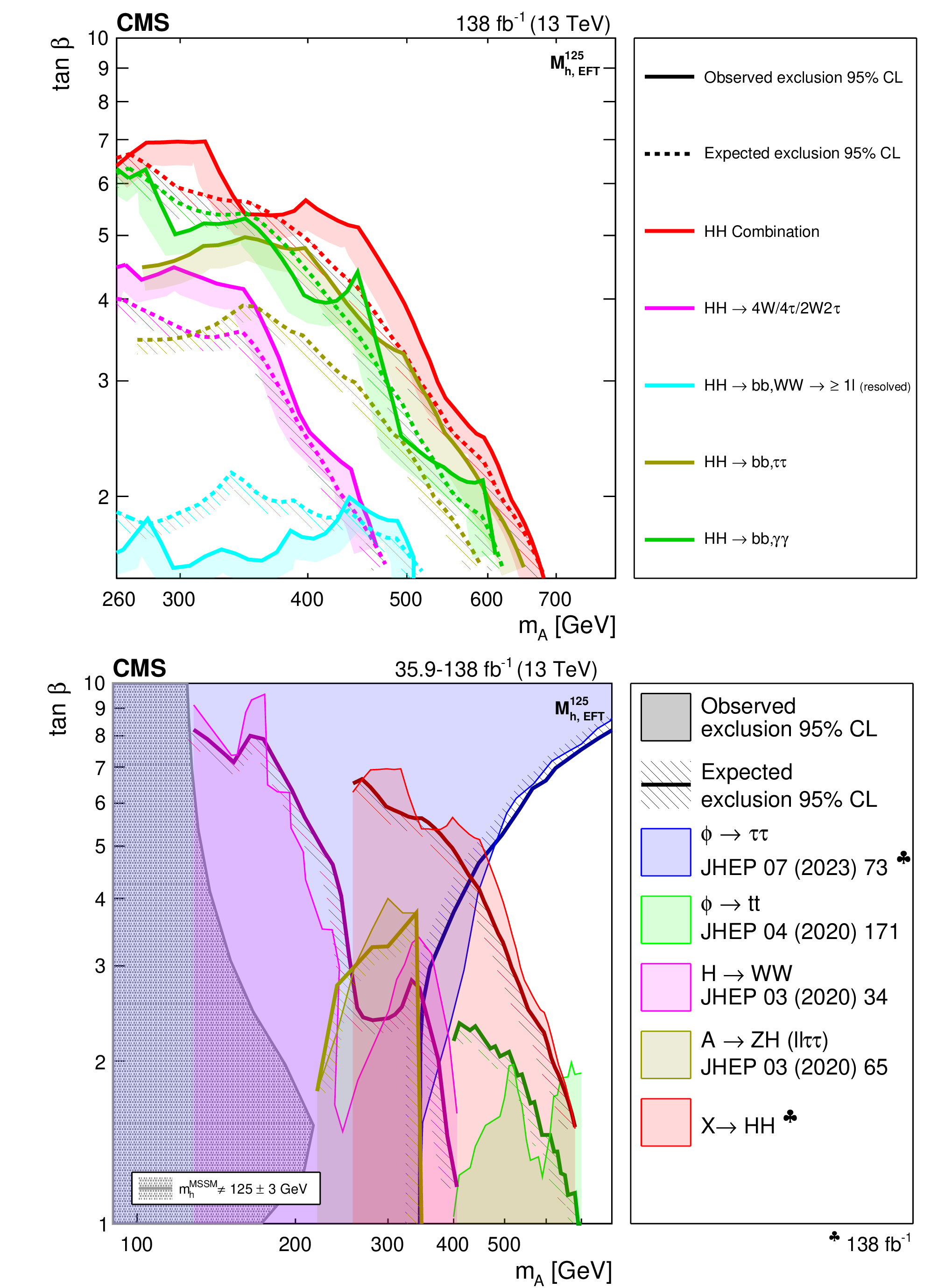
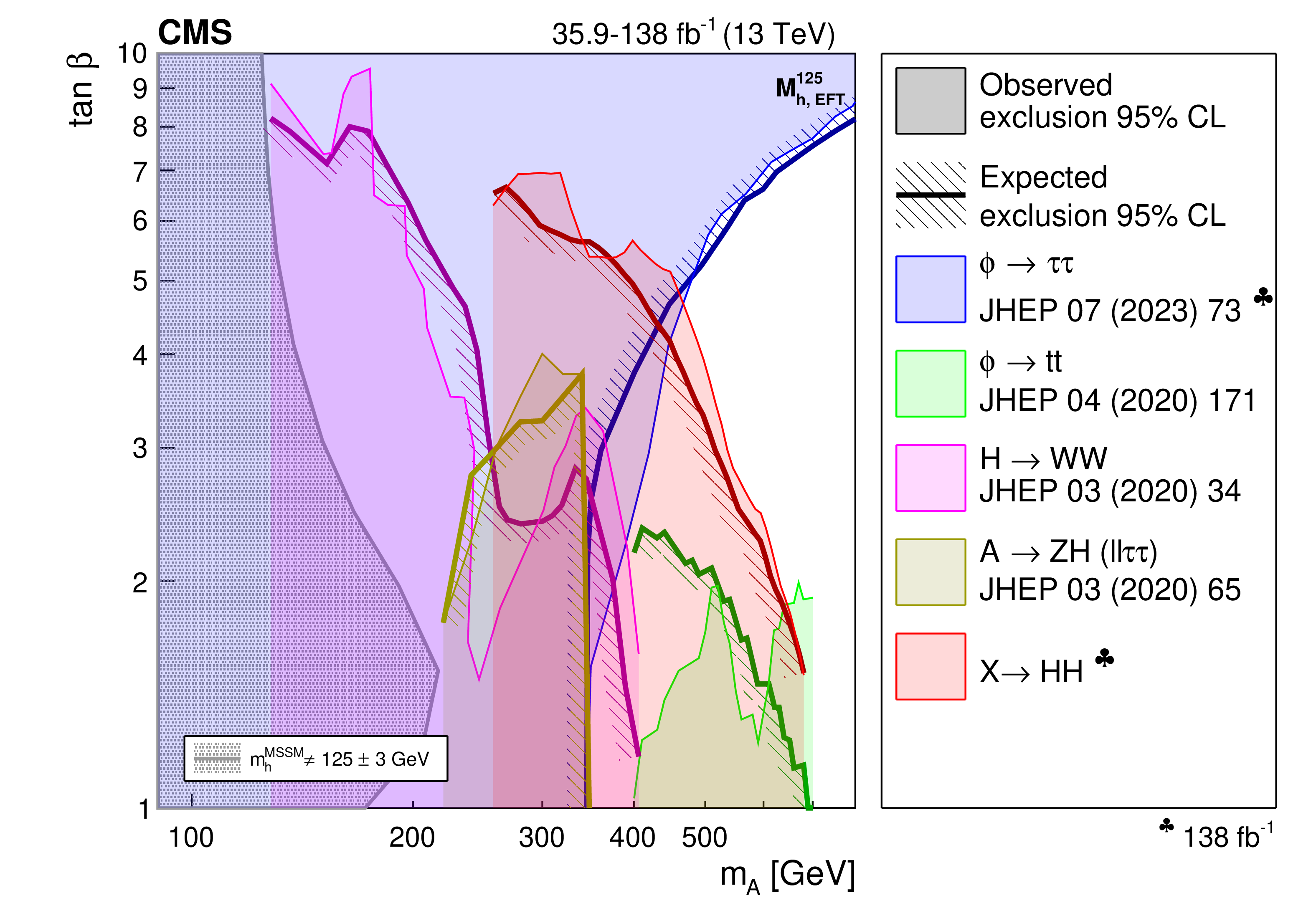
png pdf	Figure 32: Interpretation of the results from the searches for the $ \mathrm{X}\to{\mathrm{H}\mathrm{H}} $ decay, in the $ M^{125}_{\text{h,EFT}} $ benchmark scenario. In the upper part of the figure, the observed and expected exclusion contours at 95% CL are shown, in the ($ m_{{\mathrm{A}}} $, $ \tan\beta $) plane from the individual HH analyses presented in this report and their combined likelihood analysis. In the lower part of the figure, a comparison of the region excluded by the combined likelihood analysis shown in the upper part of the figure with selected results from other searches for the production of heavy scalar bosons in the $ M^{125}_{\text{h,EFT}} $ scenario, in $ \tau\tau $ [64], $ \mathrm{t} \overline{\mathrm{t}} $ [169] and WW [170] decays is shown. Also shown, are the results from one representative search for $ {\mathrm{A}}\to\mathrm{Z}\mathrm{H} $ [107]. The parameter region in which the mass of the lightest MSSM Higgs boson does not coincide with 125 GeV within a 3 GeV margin is indicated by the dark hatched area. Results not marked by a club symbol are based on an integrated luminosity of 35.9 fb$^{-1}$.
png pdf	Figure 32-a: Interpretation of the results from the searches for the $ \mathrm{X}\to{\mathrm{H}\mathrm{H}} $ decay, in the $ M^{125}_{\text{h,EFT}} $ benchmark scenario. In the upper part of the figure, the observed and expected exclusion contours at 95% CL are shown, in the ($ m_{{\mathrm{A}}} $, $ \tan\beta $) plane from the individual HH analyses presented in this report and their combined likelihood analysis. In the lower part of the figure, a comparison of the region excluded by the combined likelihood analysis shown in the upper part of the figure with selected results from other searches for the production of heavy scalar bosons in the $ M^{125}_{\text{h,EFT}} $ scenario, in $ \tau\tau $ [64], $ \mathrm{t} \overline{\mathrm{t}} $ [169] and WW [170] decays is shown. Also shown, are the results from one representative search for $ {\mathrm{A}}\to\mathrm{Z}\mathrm{H} $ [107]. The parameter region in which the mass of the lightest MSSM Higgs boson does not coincide with 125 GeV within a 3 GeV margin is indicated by the dark hatched area. Results not marked by a club symbol are based on an integrated luminosity of 35.9 fb$^{-1}$.
png pdf	Figure 32-b: Interpretation of the results from the searches for the $ \mathrm{X}\to{\mathrm{H}\mathrm{H}} $ decay, in the $ M^{125}_{\text{h,EFT}} $ benchmark scenario. In the upper part of the figure, the observed and expected exclusion contours at 95% CL are shown, in the ($ m_{{\mathrm{A}}} $, $ \tan\beta $) plane from the individual HH analyses presented in this report and their combined likelihood analysis. In the lower part of the figure, a comparison of the region excluded by the combined likelihood analysis shown in the upper part of the figure with selected results from other searches for the production of heavy scalar bosons in the $ M^{125}_{\text{h,EFT}} $ scenario, in $ \tau\tau $ [64], $ \mathrm{t} \overline{\mathrm{t}} $ [169] and WW [170] decays is shown. Also shown, are the results from one representative search for $ {\mathrm{A}}\to\mathrm{Z}\mathrm{H} $ [107]. The parameter region in which the mass of the lightest MSSM Higgs boson does not coincide with 125 GeV within a 3 GeV margin is indicated by the dark hatched area. Results not marked by a club symbol are based on an integrated luminosity of 35.9 fb$^{-1}$.
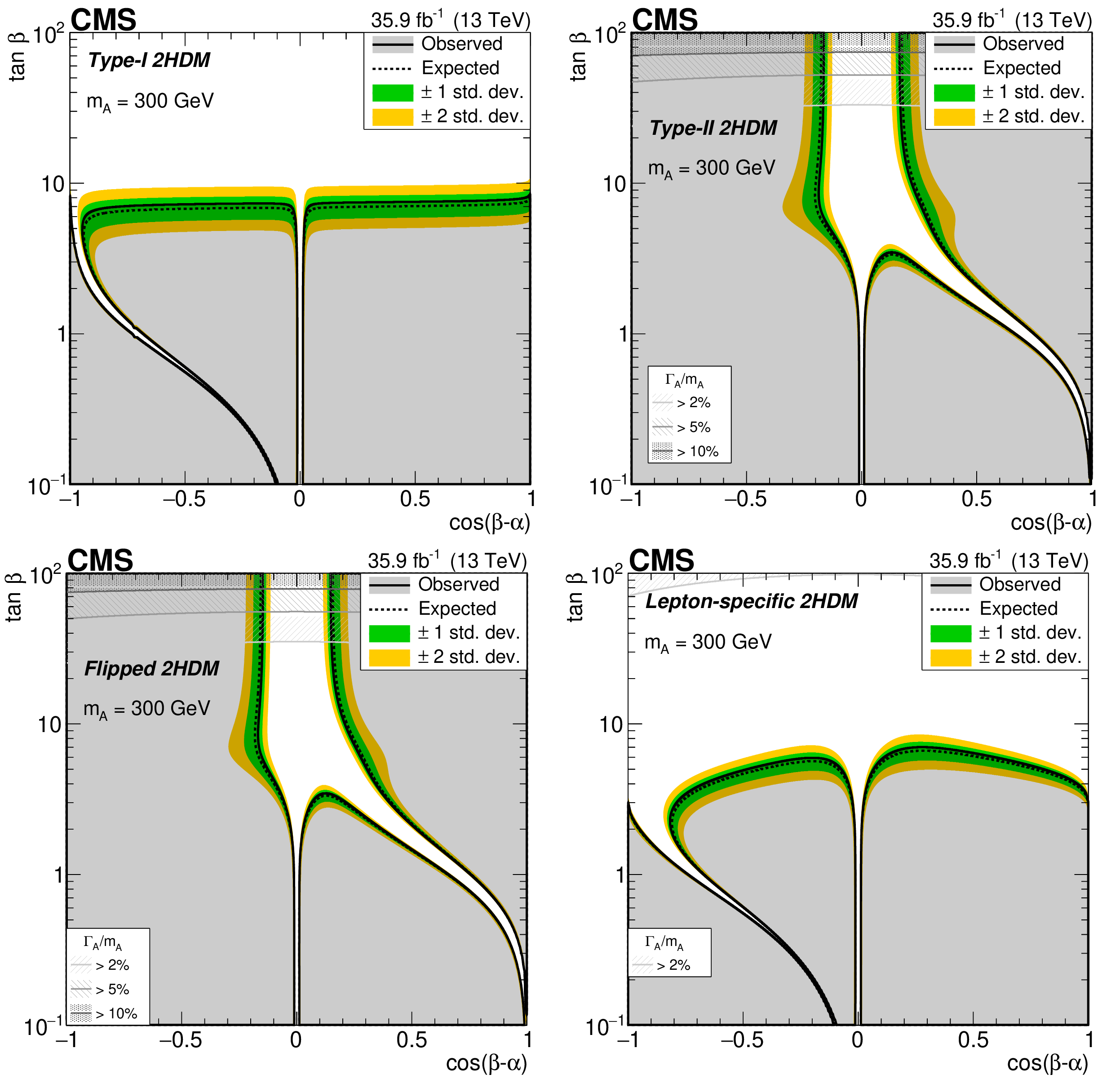
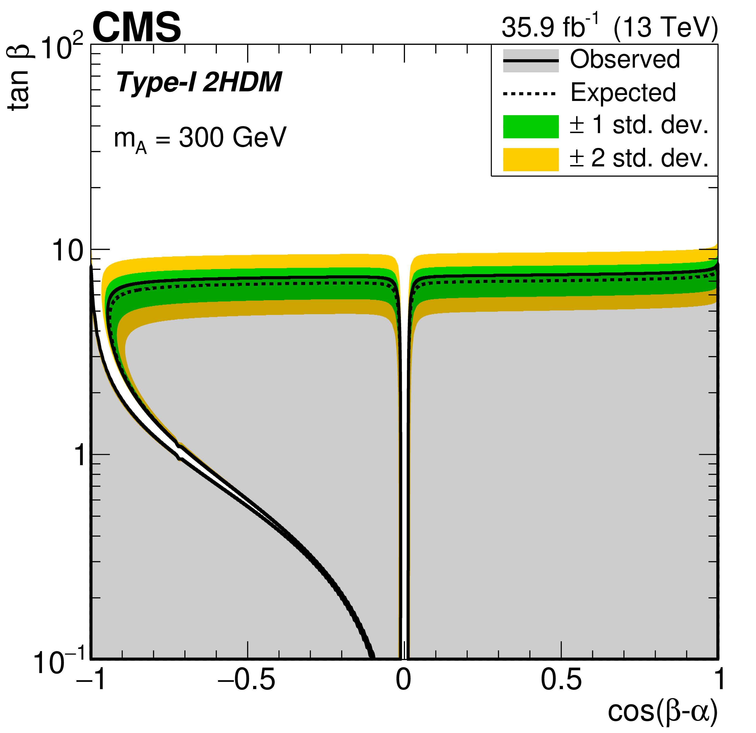
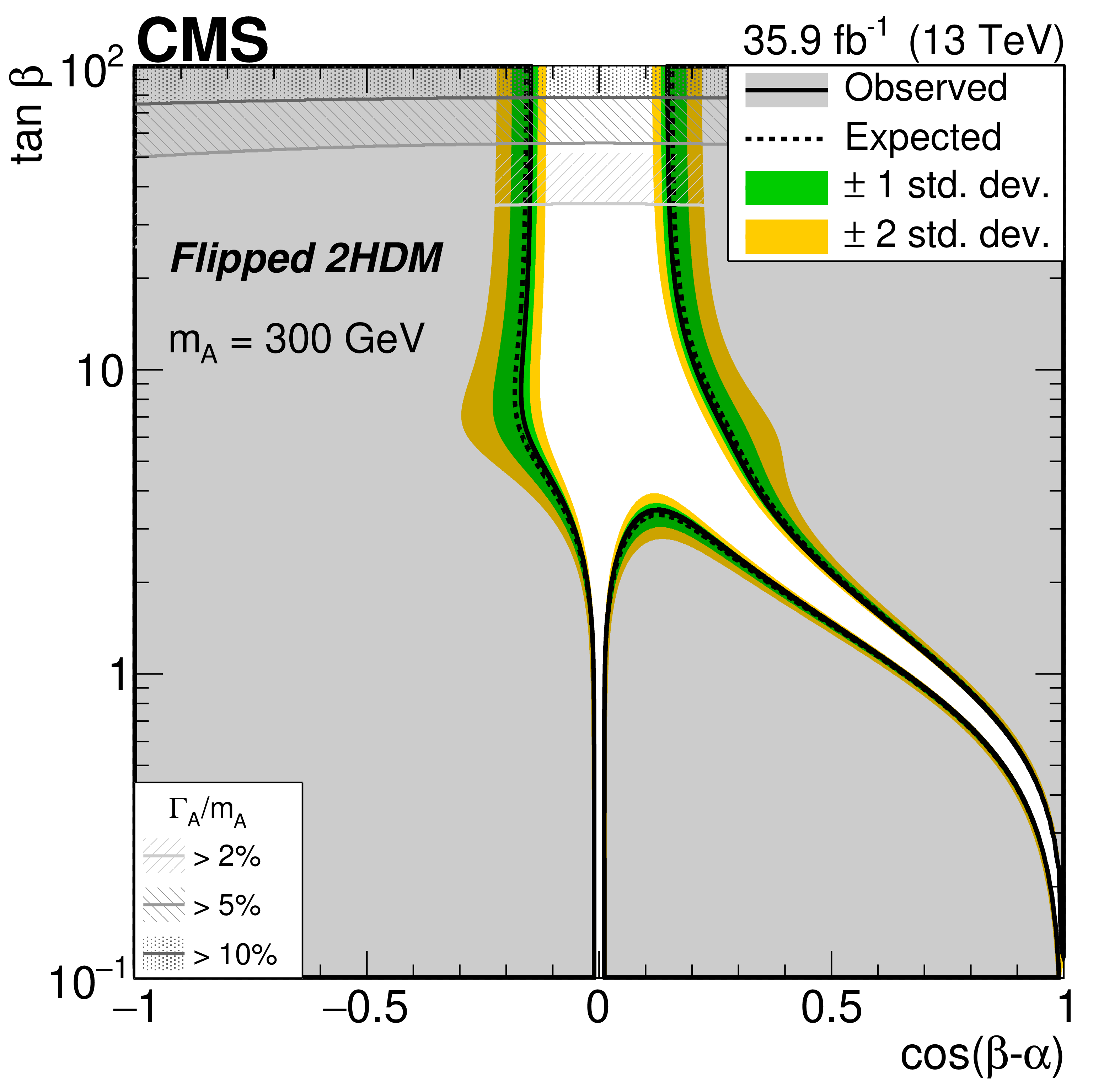
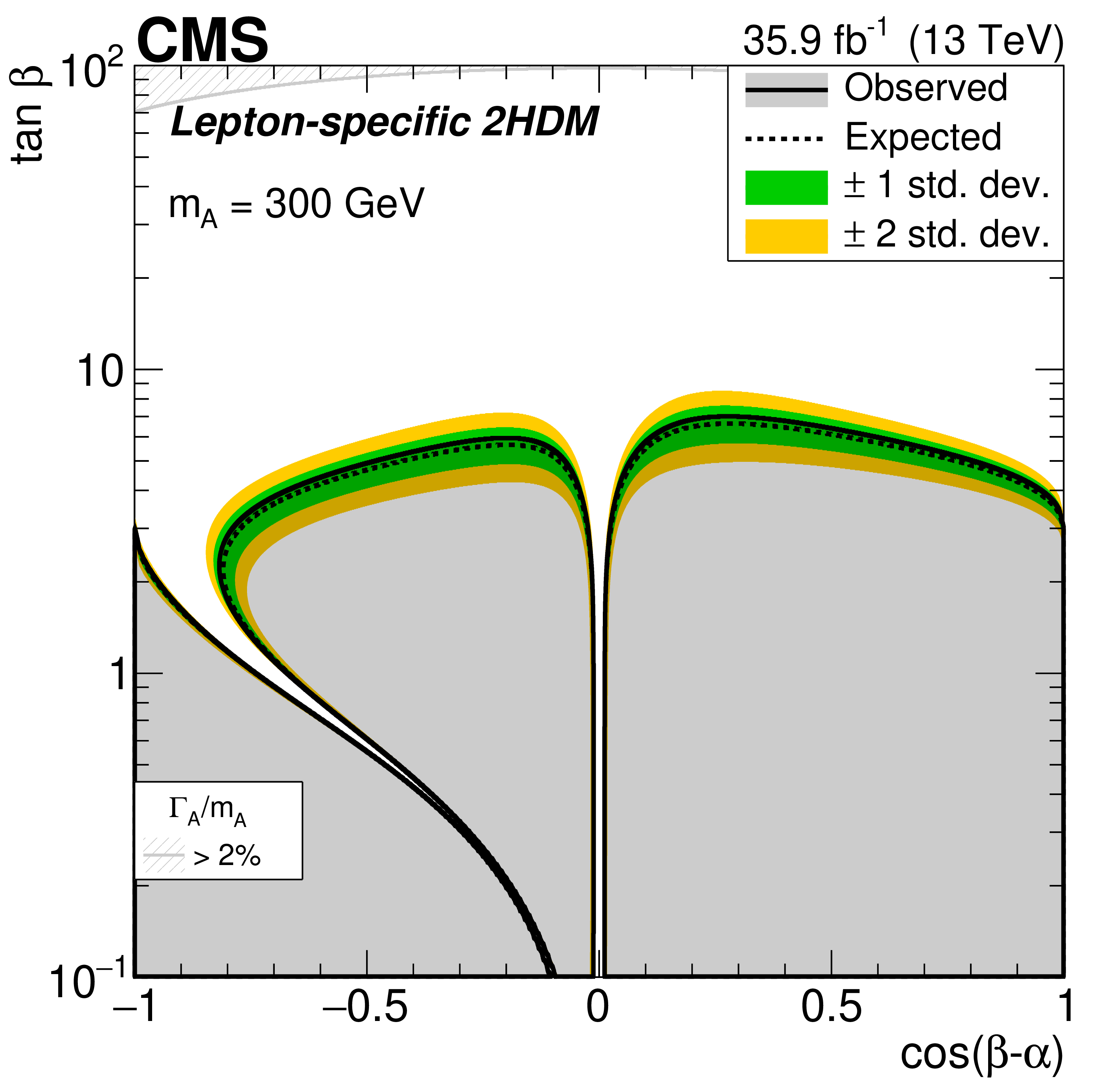
png pdf	Figure 33: Interpretation of the results of the $ {\mathrm{A}}\to\mathrm{Z}\mathrm{H}(\mathrm{b}\mathrm{b}) $ analysis [108], in the (upper left) Type I, (upper right) Type II, (lower left) flipped, and (lower right) lepton-specific 2HDM models. In each case observed and expected exclusion contours at 95% CL, in the plane defined by $ \cos(\beta-\alpha) $ and $ \tan\beta $, are shown. The excluded regions are represented by the shaded gray areas. The 68 and 95% central intervals of the expected exclusion contours in the absence of a signal are indicated by the green and yellow bands. Contours are derived from the projection on the corresponding 2HDM parameter space for $ m_{{\mathrm{A}}} = $ 300 GeV. The regions of parameter space where the natural width of the $ {\mathrm{A}} $ boson $ \Gamma_{\mathrm{A}} $ is comparable to or larger than the experimental resolution and thus the narrow-width approximation is not valid are represented by hatched gray areas. Figure from Ref. [108].
png pdf	Figure 33-a: Interpretation of the results of the $ {\mathrm{A}}\to\mathrm{Z}\mathrm{H}(\mathrm{b}\mathrm{b}) $ analysis [108], in the (upper left) Type I, (upper right) Type II, (lower left) flipped, and (lower right) lepton-specific 2HDM models. In each case observed and expected exclusion contours at 95% CL, in the plane defined by $ \cos(\beta-\alpha) $ and $ \tan\beta $, are shown. The excluded regions are represented by the shaded gray areas. The 68 and 95% central intervals of the expected exclusion contours in the absence of a signal are indicated by the green and yellow bands. Contours are derived from the projection on the corresponding 2HDM parameter space for $ m_{{\mathrm{A}}} = $ 300 GeV. The regions of parameter space where the natural width of the $ {\mathrm{A}} $ boson $ \Gamma_{\mathrm{A}} $ is comparable to or larger than the experimental resolution and thus the narrow-width approximation is not valid are represented by hatched gray areas. Figure from Ref. [108].
png pdf	Figure 33-b: Interpretation of the results of the $ {\mathrm{A}}\to\mathrm{Z}\mathrm{H}(\mathrm{b}\mathrm{b}) $ analysis [108], in the (upper left) Type I, (upper right) Type II, (lower left) flipped, and (lower right) lepton-specific 2HDM models. In each case observed and expected exclusion contours at 95% CL, in the plane defined by $ \cos(\beta-\alpha) $ and $ \tan\beta $, are shown. The excluded regions are represented by the shaded gray areas. The 68 and 95% central intervals of the expected exclusion contours in the absence of a signal are indicated by the green and yellow bands. Contours are derived from the projection on the corresponding 2HDM parameter space for $ m_{{\mathrm{A}}} = $ 300 GeV. The regions of parameter space where the natural width of the $ {\mathrm{A}} $ boson $ \Gamma_{\mathrm{A}} $ is comparable to or larger than the experimental resolution and thus the narrow-width approximation is not valid are represented by hatched gray areas. Figure from Ref. [108].
png pdf	Figure 33-c: Interpretation of the results of the $ {\mathrm{A}}\to\mathrm{Z}\mathrm{H}(\mathrm{b}\mathrm{b}) $ analysis [108], in the (upper left) Type I, (upper right) Type II, (lower left) flipped, and (lower right) lepton-specific 2HDM models. In each case observed and expected exclusion contours at 95% CL, in the plane defined by $ \cos(\beta-\alpha) $ and $ \tan\beta $, are shown. The excluded regions are represented by the shaded gray areas. The 68 and 95% central intervals of the expected exclusion contours in the absence of a signal are indicated by the green and yellow bands. Contours are derived from the projection on the corresponding 2HDM parameter space for $ m_{{\mathrm{A}}} = $ 300 GeV. The regions of parameter space where the natural width of the $ {\mathrm{A}} $ boson $ \Gamma_{\mathrm{A}} $ is comparable to or larger than the experimental resolution and thus the narrow-width approximation is not valid are represented by hatched gray areas. Figure from Ref. [108].
png pdf	Figure 33-d: Interpretation of the results of the $ {\mathrm{A}}\to\mathrm{Z}\mathrm{H}(\mathrm{b}\mathrm{b}) $ analysis [108], in the (upper left) Type I, (upper right) Type II, (lower left) flipped, and (lower right) lepton-specific 2HDM models. In each case observed and expected exclusion contours at 95% CL, in the plane defined by $ \cos(\beta-\alpha) $ and $ \tan\beta $, are shown. The excluded regions are represented by the shaded gray areas. The 68 and 95% central intervals of the expected exclusion contours in the absence of a signal are indicated by the green and yellow bands. Contours are derived from the projection on the corresponding 2HDM parameter space for $ m_{{\mathrm{A}}} = $ 300 GeV. The regions of parameter space where the natural width of the $ {\mathrm{A}} $ boson $ \Gamma_{\mathrm{A}} $ is comparable to or larger than the experimental resolution and thus the narrow-width approximation is not valid are represented by hatched gray areas. Figure from Ref. [108].
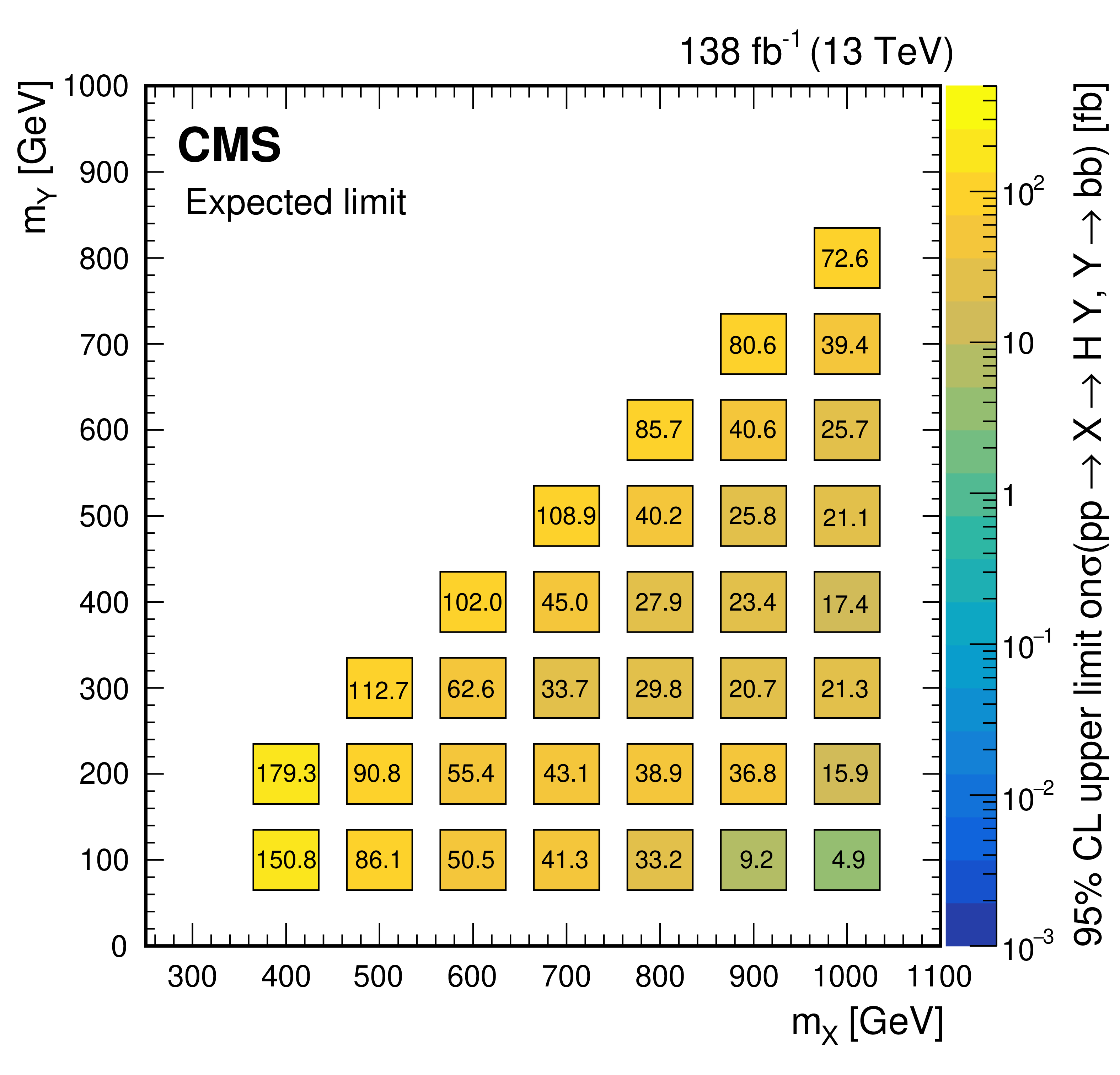
png pdf	Figure 34: (Upper left) Observed and (upper right) expected upper limits at 95% CL, on the product of the cross section $ \sigma $ for the production of a resonance X via gluon-gluon fusion and the branching fraction $ \mathcal{B} $ for the $ \mathrm{X}\to{\mathrm{Y}}(\mathrm{b}\mathrm{b})\mathrm{H} $ decay, as obtained from a combined likelihood analysis of the individual analyses presented in this report and shown in Fig. 29. The results are presented in a plane defined by $ m_{\mathrm{X}} $ and $ m_{{\mathrm{Y}}} $. The limits have been evaluated in discrete steps corresponding to the centers of the boxes. The numbers in the boxes are given in fb. The corresponding maximally allowed values of $ \sigma\mathcal{B} $ in the NMSSM are also shown for comparison (lower plot), as adapted from Ref. [193].
png pdf	Figure 34-a: (Upper left) Observed and (upper right) expected upper limits at 95% CL, on the product of the cross section $ \sigma $ for the production of a resonance X via gluon-gluon fusion and the branching fraction $ \mathcal{B} $ for the $ \mathrm{X}\to{\mathrm{Y}}(\mathrm{b}\mathrm{b})\mathrm{H} $ decay, as obtained from a combined likelihood analysis of the individual analyses presented in this report and shown in Fig. 29. The results are presented in a plane defined by $ m_{\mathrm{X}} $ and $ m_{{\mathrm{Y}}} $. The limits have been evaluated in discrete steps corresponding to the centers of the boxes. The numbers in the boxes are given in fb. The corresponding maximally allowed values of $ \sigma\mathcal{B} $ in the NMSSM are also shown for comparison (lower plot), as adapted from Ref. [193].
png pdf	Figure 34-b: (Upper left) Observed and (upper right) expected upper limits at 95% CL, on the product of the cross section $ \sigma $ for the production of a resonance X via gluon-gluon fusion and the branching fraction $ \mathcal{B} $ for the $ \mathrm{X}\to{\mathrm{Y}}(\mathrm{b}\mathrm{b})\mathrm{H} $ decay, as obtained from a combined likelihood analysis of the individual analyses presented in this report and shown in Fig. 29. The results are presented in a plane defined by $ m_{\mathrm{X}} $ and $ m_{{\mathrm{Y}}} $. The limits have been evaluated in discrete steps corresponding to the centers of the boxes. The numbers in the boxes are given in fb. The corresponding maximally allowed values of $ \sigma\mathcal{B} $ in the NMSSM are also shown for comparison (lower plot), as adapted from Ref. [193].
png pdf	Figure 34-c: (Upper left) Observed and (upper right) expected upper limits at 95% CL, on the product of the cross section $ \sigma $ for the production of a resonance X via gluon-gluon fusion and the branching fraction $ \mathcal{B} $ for the $ \mathrm{X}\to{\mathrm{Y}}(\mathrm{b}\mathrm{b})\mathrm{H} $ decay, as obtained from a combined likelihood analysis of the individual analyses presented in this report and shown in Fig. 29. The results are presented in a plane defined by $ m_{\mathrm{X}} $ and $ m_{{\mathrm{Y}}} $. The limits have been evaluated in discrete steps corresponding to the centers of the boxes. The numbers in the boxes are given in fb. The corresponding maximally allowed values of $ \sigma\mathcal{B} $ in the NMSSM are also shown for comparison (lower plot), as adapted from Ref. [193].
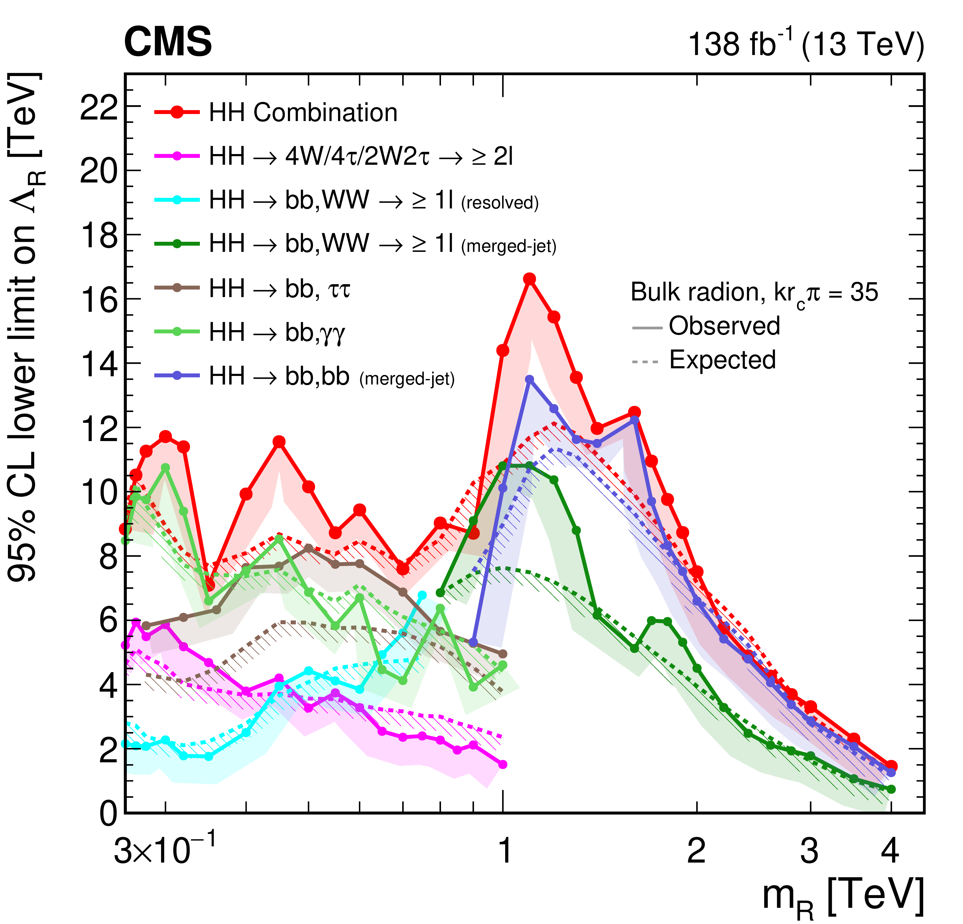
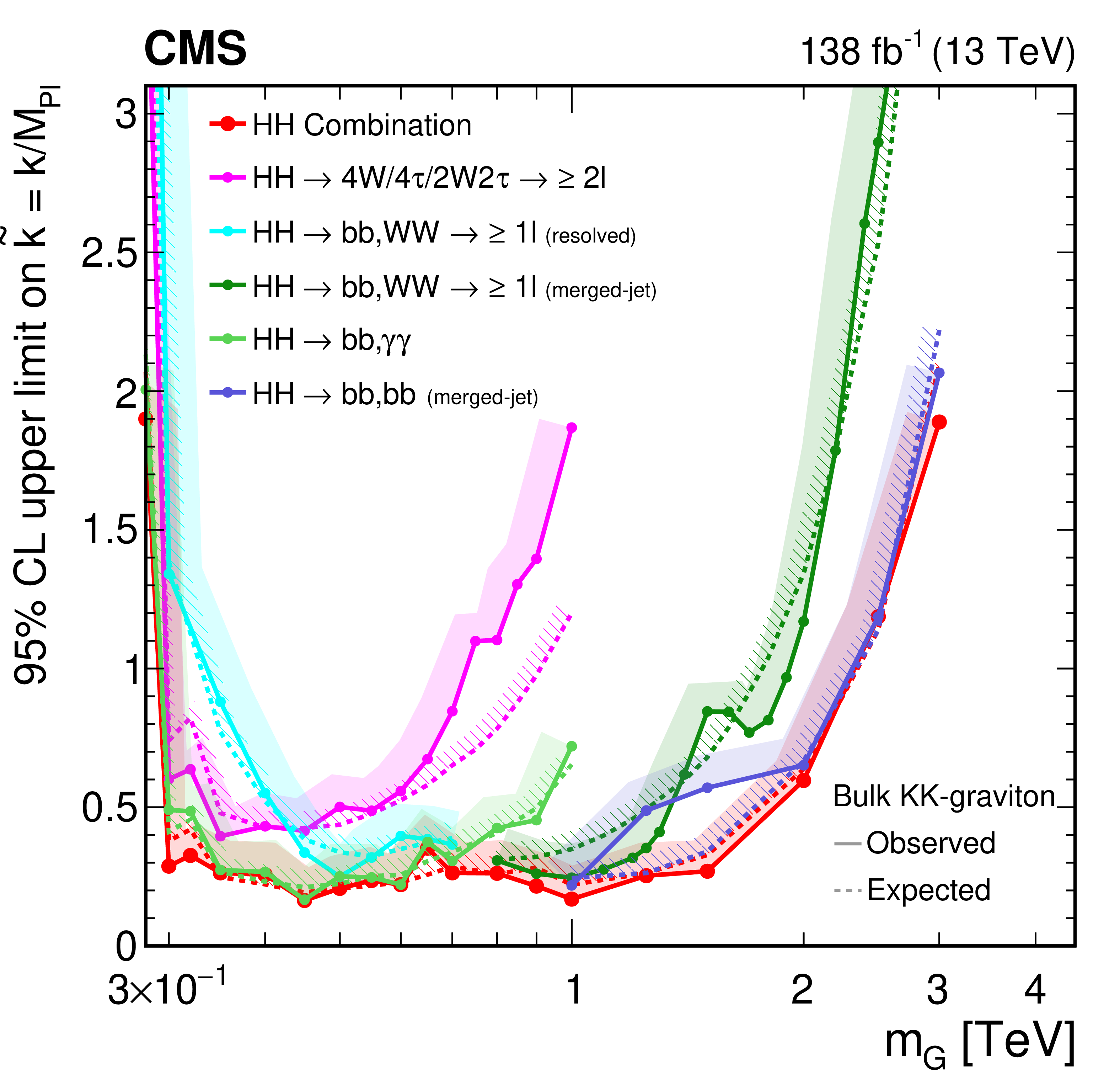
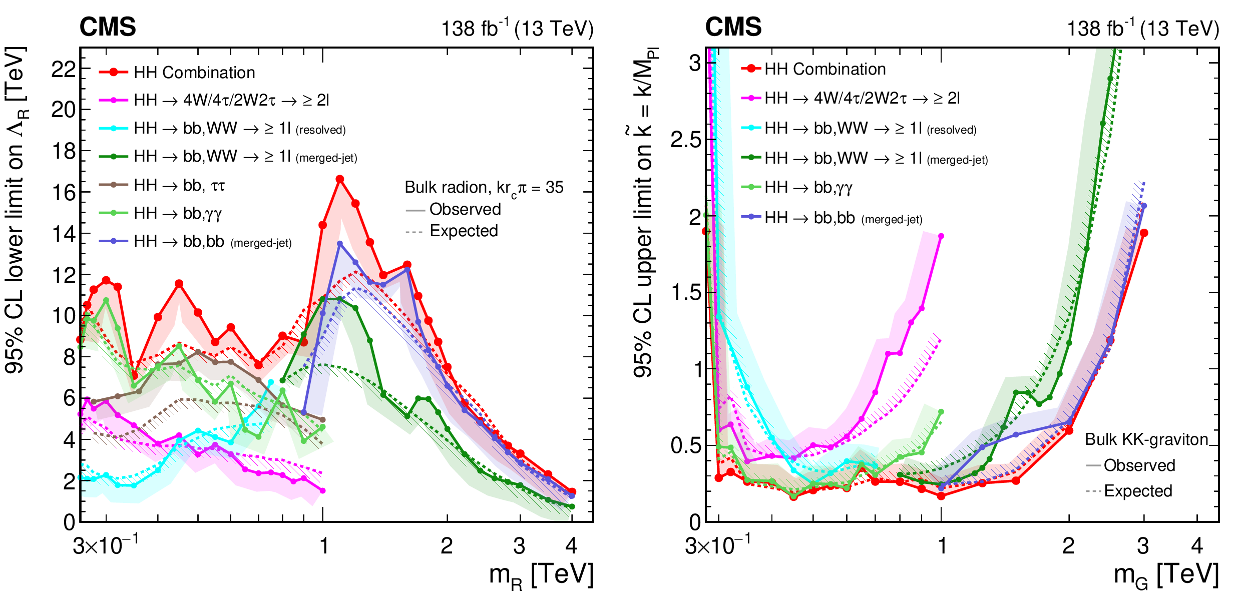
png pdf	Figure 35: Observed and expected limits, at 95% CL, on the parameters of models with warped extra dimensions, as obtained from the $ \mathrm{X}\to\mathrm{H}\mathrm{H} $ analyses presented in this report and their combined likelihood analysis. Shown are lower limits (left) on the bulk radion ultraviolet cutoff parameter $ \Lambda_{\mathrm{R}} $, as a function of the radion mass $ m_{{\mathrm{R}} } $, and upper limits (right) on the parameter $ \tilde{k} $ of the spin-2 bulk graviton G, as a function of $ m_{{\mathrm{G}} } $. Excluded areas are indicated by the direction of the hatching along the exclusion contours.
png pdf	Figure 35-a: Observed and expected limits, at 95% CL, on the parameters of models with warped extra dimensions, as obtained from the $ \mathrm{X}\to\mathrm{H}\mathrm{H} $ analyses presented in this report and their combined likelihood analysis. Shown are lower limits (left) on the bulk radion ultraviolet cutoff parameter $ \Lambda_{\mathrm{R}} $, as a function of the radion mass $ m_{{\mathrm{R}} } $, and upper limits (right) on the parameter $ \tilde{k} $ of the spin-2 bulk graviton G, as a function of $ m_{{\mathrm{G}} } $. Excluded areas are indicated by the direction of the hatching along the exclusion contours.
png pdf	Figure 35-b: Observed and expected limits, at 95% CL, on the parameters of models with warped extra dimensions, as obtained from the $ \mathrm{X}\to\mathrm{H}\mathrm{H} $ analyses presented in this report and their combined likelihood analysis. Shown are lower limits (left) on the bulk radion ultraviolet cutoff parameter $ \Lambda_{\mathrm{R}} $, as a function of the radion mass $ m_{{\mathrm{R}} } $, and upper limits (right) on the parameter $ \tilde{k} $ of the spin-2 bulk graviton G, as a function of $ m_{{\mathrm{G}} } $. Excluded areas are indicated by the direction of the hatching along the exclusion contours.
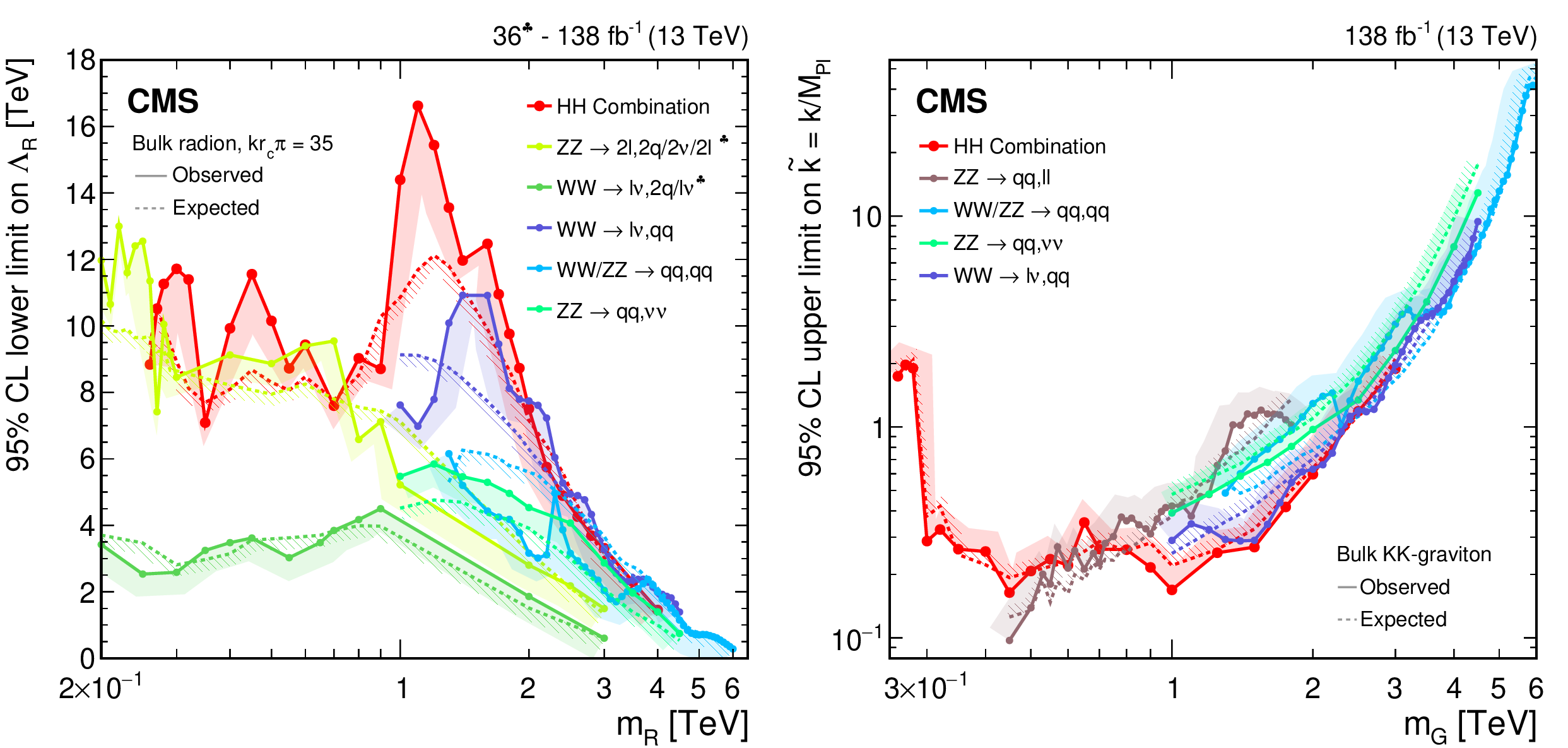
png pdf	Figure 36: Observed and expected limits, at 95% CL, on the parameters of models with warped extra dimensions, as obtained from the combined likelihood analysis of the individual $ \mathrm{X}\to\mathrm{H}\mathrm{H} $ analyses presented in this report and shown in Fig. 35. The exclusion contours obtained from the combined likelihood analysis are compared to similar exclusions obtained from individual searches in the decays $ \mathrm{Z}(\ell\ell)\mathrm{Z}(\mathrm{q}\mathrm{q}/\nu\nu/\ell\ell) $ [195], $ \mathrm{W}(\ell\nu)\mathrm{W}(\ell\nu/\mathrm{q}\mathrm{q}) $ [170], $ \mathrm{W}(\ell\nu)\mathrm{W}(\mathrm{q}\mathrm{q}) $ [109], $ \mathrm{V}(\mathrm{q}\mathrm{q})\mathrm{V}(\mathrm{q}\mathrm{q}) $ [111], and $ \mathrm{Z}(\nu\nu)\mathrm{Z}(\mathrm{q}\mathrm{q}) $ [196], in case of the radion interpretation, and from individual searches in the decays $ \mathrm{Z}(\mathrm{q}\mathrm{q})\mathrm{Z}(\ell\ell) $ [197], $ \mathrm{V}(\mathrm{q}\mathrm{q})\mathrm{V}(\mathrm{q}\mathrm{q}) $ [111], $ \mathrm{Z}(\nu\nu)\mathrm{Z}(\mathrm{q}\mathrm{q}) $ [196], and $ \mathrm{W}(\ell\nu)\mathrm{W}(\mathrm{q}\mathrm{q}) $ [109], in the case of the graviton interpretation. Excluded areas are indicated by the direction of the hatching along the exclusion contours.
png pdf	Figure 36-a: Observed and expected limits, at 95% CL, on the parameters of models with warped extra dimensions, as obtained from the combined likelihood analysis of the individual $ \mathrm{X}\to\mathrm{H}\mathrm{H} $ analyses presented in this report and shown in Fig. 35. The exclusion contours obtained from the combined likelihood analysis are compared to similar exclusions obtained from individual searches in the decays $ \mathrm{Z}(\ell\ell)\mathrm{Z}(\mathrm{q}\mathrm{q}/\nu\nu/\ell\ell) $ [195], $ \mathrm{W}(\ell\nu)\mathrm{W}(\ell\nu/\mathrm{q}\mathrm{q}) $ [170], $ \mathrm{W}(\ell\nu)\mathrm{W}(\mathrm{q}\mathrm{q}) $ [109], $ \mathrm{V}(\mathrm{q}\mathrm{q})\mathrm{V}(\mathrm{q}\mathrm{q}) $ [111], and $ \mathrm{Z}(\nu\nu)\mathrm{Z}(\mathrm{q}\mathrm{q}) $ [196], in case of the radion interpretation, and from individual searches in the decays $ \mathrm{Z}(\mathrm{q}\mathrm{q})\mathrm{Z}(\ell\ell) $ [197], $ \mathrm{V}(\mathrm{q}\mathrm{q})\mathrm{V}(\mathrm{q}\mathrm{q}) $ [111], $ \mathrm{Z}(\nu\nu)\mathrm{Z}(\mathrm{q}\mathrm{q}) $ [196], and $ \mathrm{W}(\ell\nu)\mathrm{W}(\mathrm{q}\mathrm{q}) $ [109], in the case of the graviton interpretation. Excluded areas are indicated by the direction of the hatching along the exclusion contours.
png pdf	Figure 36-b: Observed and expected limits, at 95% CL, on the parameters of models with warped extra dimensions, as obtained from the combined likelihood analysis of the individual $ \mathrm{X}\to\mathrm{H}\mathrm{H} $ analyses presented in this report and shown in Fig. 35. The exclusion contours obtained from the combined likelihood analysis are compared to similar exclusions obtained from individual searches in the decays $ \mathrm{Z}(\ell\ell)\mathrm{Z}(\mathrm{q}\mathrm{q}/\nu\nu/\ell\ell) $ [195], $ \mathrm{W}(\ell\nu)\mathrm{W}(\ell\nu/\mathrm{q}\mathrm{q}) $ [170], $ \mathrm{W}(\ell\nu)\mathrm{W}(\mathrm{q}\mathrm{q}) $ [109], $ \mathrm{V}(\mathrm{q}\mathrm{q})\mathrm{V}(\mathrm{q}\mathrm{q}) $ [111], and $ \mathrm{Z}(\nu\nu)\mathrm{Z}(\mathrm{q}\mathrm{q}) $ [196], in case of the radion interpretation, and from individual searches in the decays $ \mathrm{Z}(\mathrm{q}\mathrm{q})\mathrm{Z}(\ell\ell) $ [197], $ \mathrm{V}(\mathrm{q}\mathrm{q})\mathrm{V}(\mathrm{q}\mathrm{q}) $ [111], $ \mathrm{Z}(\nu\nu)\mathrm{Z}(\mathrm{q}\mathrm{q}) $ [196], and $ \mathrm{W}(\ell\nu)\mathrm{W}(\mathrm{q}\mathrm{q}) $ [109], in the case of the graviton interpretation. Excluded areas are indicated by the direction of the hatching along the exclusion contours.
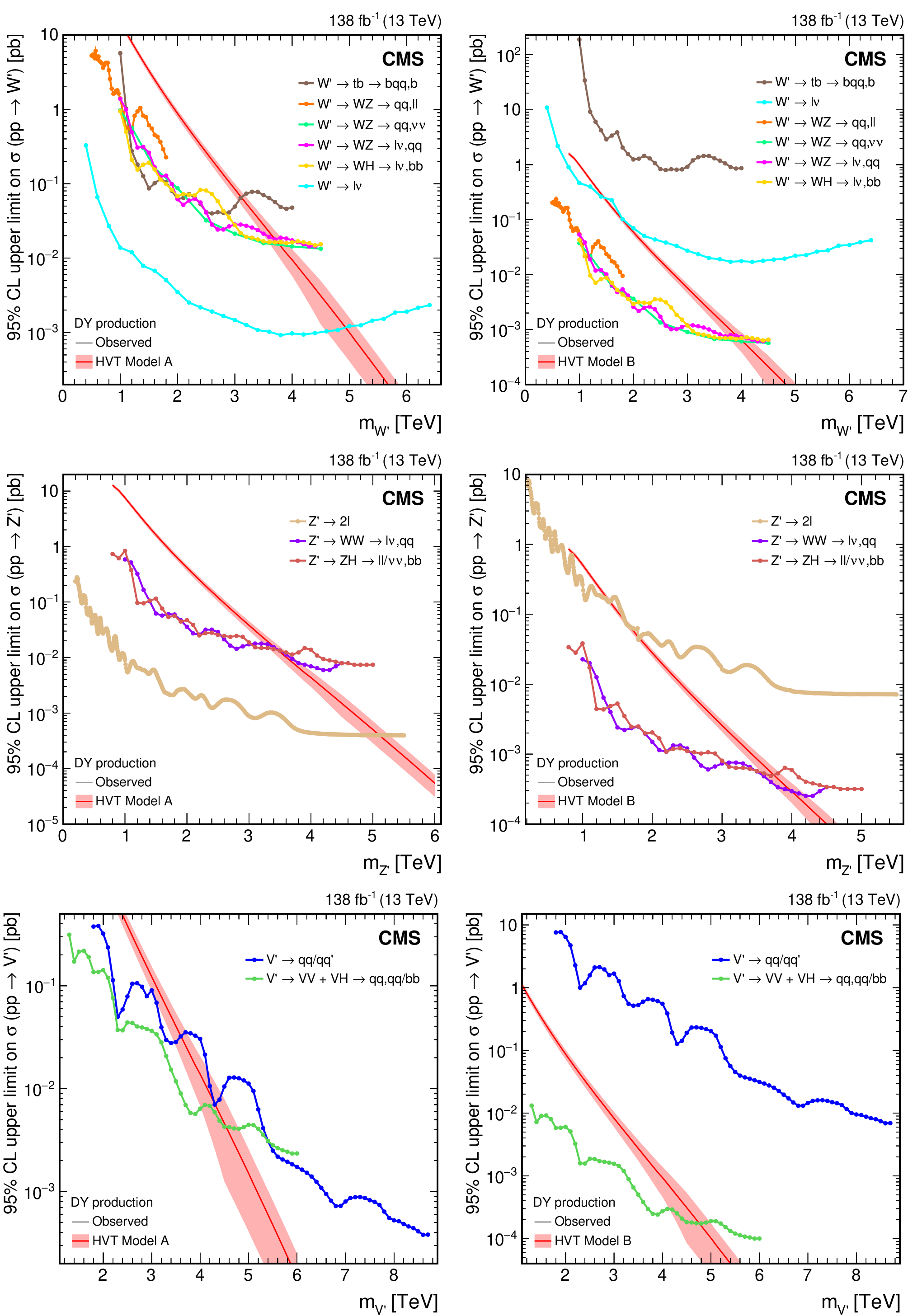
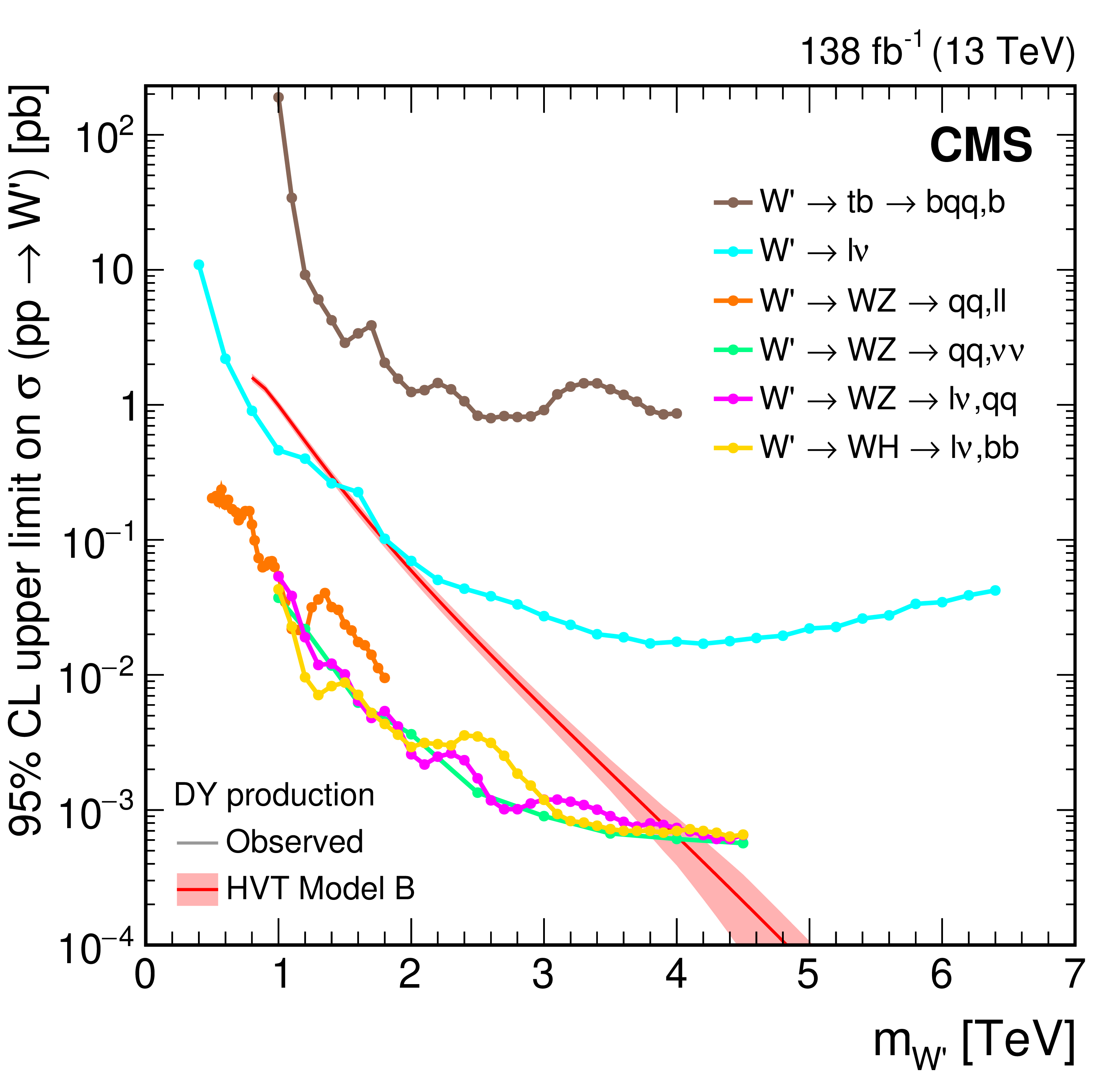
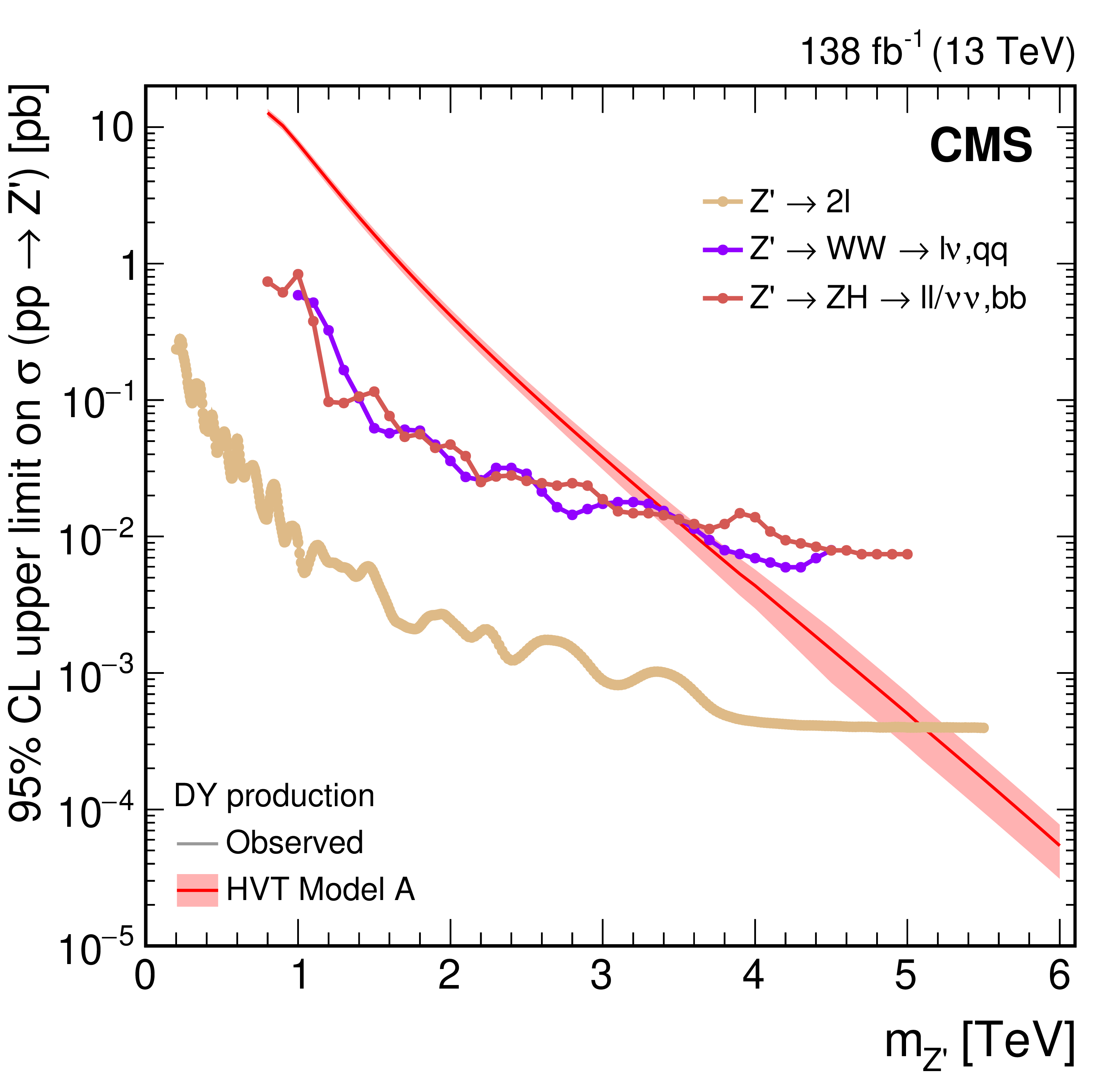
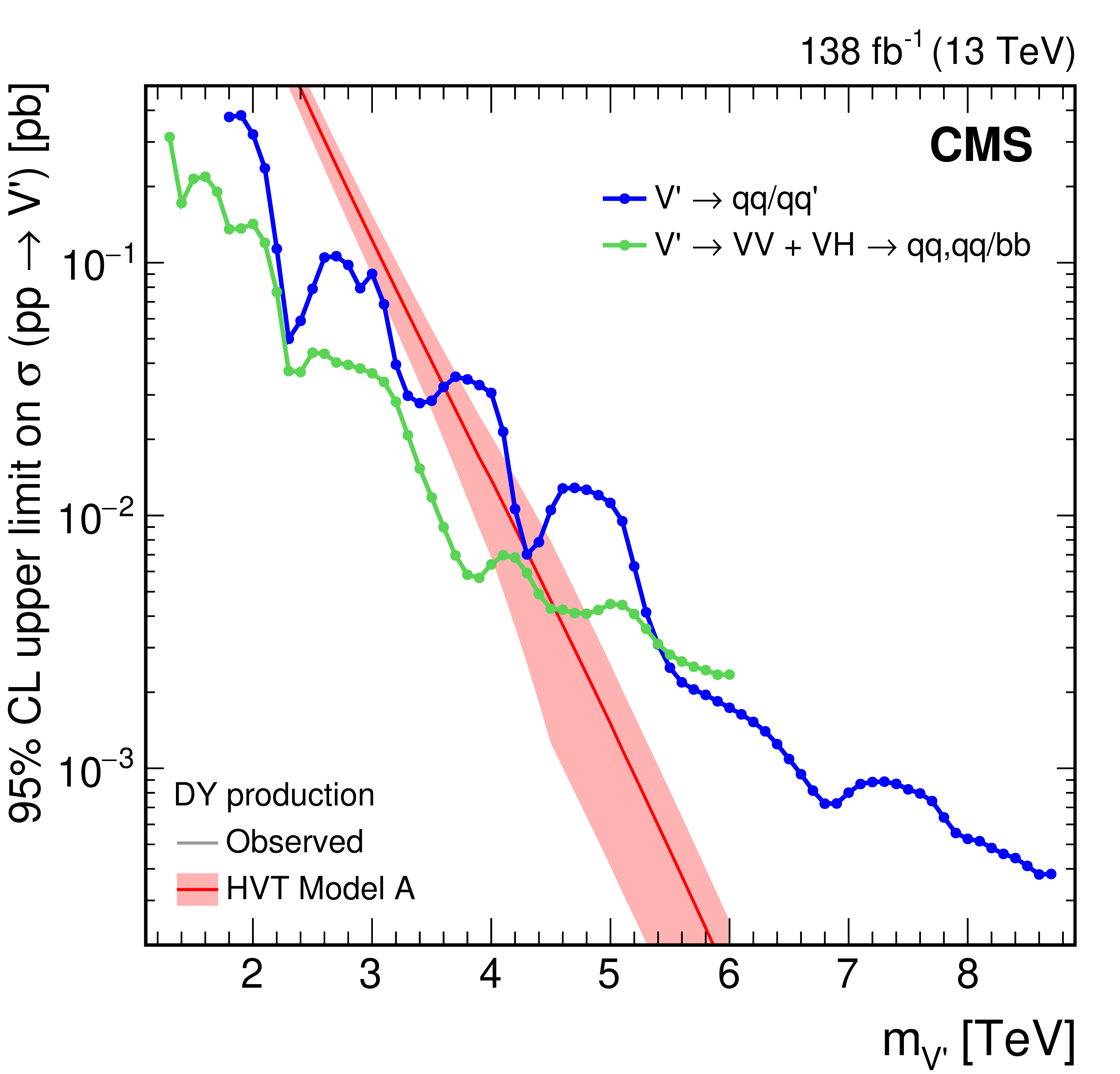
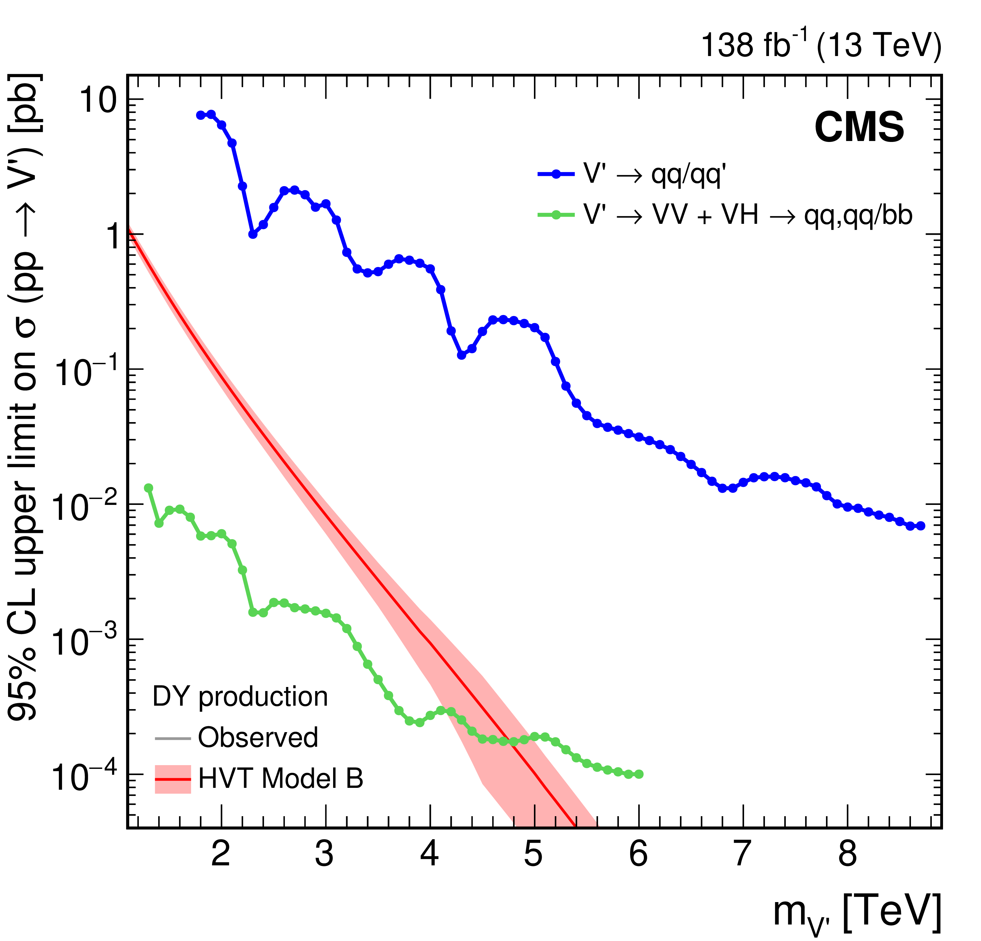
png pdf	Figure 37: Observed upper limits, at 95% CL, on the Drell-Yan production cross section of (upper) W', (middle) Z', and (lower) combined $ \mathrm{V}^{\prime} $ spin-1 resonances assuming branching fractions of the heavy vector triplet models (left) A and (right) B. The theory predictions from these models are also shown. Results from the VH [109,110,111] and VV channels [109,111,197,196], as well as results from dijet [201], $ \mathrm{t}\mathrm{b} $ [199], $ \ell\ell $ [198], and $ \ell\nu $ [200] final states are also shown, for comparison.
png pdf	Figure 37-a: Observed upper limits, at 95% CL, on the Drell-Yan production cross section of (upper) W', (middle) Z', and (lower) combined $ \mathrm{V}^{\prime} $ spin-1 resonances assuming branching fractions of the heavy vector triplet models (left) A and (right) B. The theory predictions from these models are also shown. Results from the VH [109,110,111] and VV channels [109,111,197,196], as well as results from dijet [201], $ \mathrm{t}\mathrm{b} $ [199], $ \ell\ell $ [198], and $ \ell\nu $ [200] final states are also shown, for comparison.
png pdf	Figure 37-b: Observed upper limits, at 95% CL, on the Drell-Yan production cross section of (upper) W', (middle) Z', and (lower) combined $ \mathrm{V}^{\prime} $ spin-1 resonances assuming branching fractions of the heavy vector triplet models (left) A and (right) B. The theory predictions from these models are also shown. Results from the VH [109,110,111] and VV channels [109,111,197,196], as well as results from dijet [201], $ \mathrm{t}\mathrm{b} $ [199], $ \ell\ell $ [198], and $ \ell\nu $ [200] final states are also shown, for comparison.
png pdf	Figure 37-c: Observed upper limits, at 95% CL, on the Drell-Yan production cross section of (upper) W', (middle) Z', and (lower) combined $ \mathrm{V}^{\prime} $ spin-1 resonances assuming branching fractions of the heavy vector triplet models (left) A and (right) B. The theory predictions from these models are also shown. Results from the VH [109,110,111] and VV channels [109,111,197,196], as well as results from dijet [201], $ \mathrm{t}\mathrm{b} $ [199], $ \ell\ell $ [198], and $ \ell\nu $ [200] final states are also shown, for comparison.
png pdf	Figure 37-d: Observed upper limits, at 95% CL, on the Drell-Yan production cross section of (upper) W', (middle) Z', and (lower) combined $ \mathrm{V}^{\prime} $ spin-1 resonances assuming branching fractions of the heavy vector triplet models (left) A and (right) B. The theory predictions from these models are also shown. Results from the VH [109,110,111] and VV channels [109,111,197,196], as well as results from dijet [201], $ \mathrm{t}\mathrm{b} $ [199], $ \ell\ell $ [198], and $ \ell\nu $ [200] final states are also shown, for comparison.
png pdf	Figure 37-e: Observed upper limits, at 95% CL, on the Drell-Yan production cross section of (upper) W', (middle) Z', and (lower) combined $ \mathrm{V}^{\prime} $ spin-1 resonances assuming branching fractions of the heavy vector triplet models (left) A and (right) B. The theory predictions from these models are also shown. Results from the VH [109,110,111] and VV channels [109,111,197,196], as well as results from dijet [201], $ \mathrm{t}\mathrm{b} $ [199], $ \ell\ell $ [198], and $ \ell\nu $ [200] final states are also shown, for comparison.
png pdf	Figure 37-f: Observed upper limits, at 95% CL, on the Drell-Yan production cross section of (upper) W', (middle) Z', and (lower) combined $ \mathrm{V}^{\prime} $ spin-1 resonances assuming branching fractions of the heavy vector triplet models (left) A and (right) B. The theory predictions from these models are also shown. Results from the VH [109,110,111] and VV channels [109,111,197,196], as well as results from dijet [201], $ \mathrm{t}\mathrm{b} $ [199], $ \ell\ell $ [198], and $ \ell\nu $ [200] final states are also shown, for comparison.
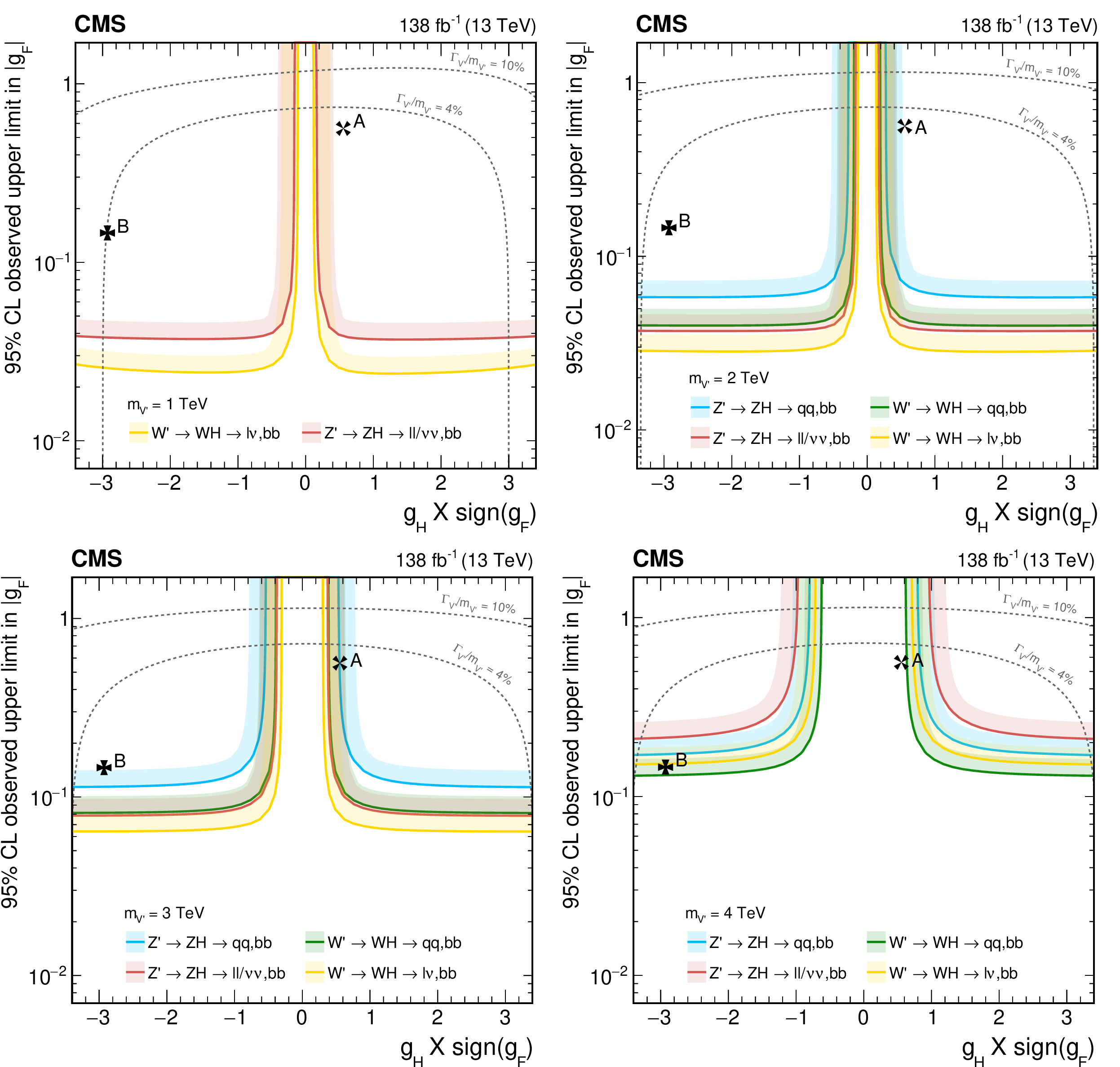
png pdf	Figure 38: Observed upper limits, at 95% CL, on the $ \mathrm{V}^{\prime} $ couplings $ g_\mathrm{F} $ and $ g_{\mathrm{H}} $ within the HVT model for $ \mathrm{V}^{\prime} $ masses of (upper left) 1, (upper right) 2, (lower left) 3, and (lower right) 4 TeV, from DY production, derived from VH channels of Refs. [109,110,111] discussed in this report. Excluded areas are indicated by the direction of the shading along the exclusion contours. The dotted lines denote coupling values above which the relative width of the resonance, $ \Gamma_{\mathrm{V}^{\prime}} /m_{V^{\prime}} $, exceeds 4 and 10%, respectively, implying that the narrow width approximation no longer applies. The couplings corresponding to the heavy vector triplet models A and B are indicated by cross markers.
png pdf	Figure 38-a: Observed upper limits, at 95% CL, on the $ \mathrm{V}^{\prime} $ couplings $ g_\mathrm{F} $ and $ g_{\mathrm{H}} $ within the HVT model for $ \mathrm{V}^{\prime} $ masses of (upper left) 1, (upper right) 2, (lower left) 3, and (lower right) 4 TeV, from DY production, derived from VH channels of Refs. [109,110,111] discussed in this report. Excluded areas are indicated by the direction of the shading along the exclusion contours. The dotted lines denote coupling values above which the relative width of the resonance, $ \Gamma_{\mathrm{V}^{\prime}} /m_{V^{\prime}} $, exceeds 4 and 10%, respectively, implying that the narrow width approximation no longer applies. The couplings corresponding to the heavy vector triplet models A and B are indicated by cross markers.
png pdf	Figure 38-b: Observed upper limits, at 95% CL, on the $ \mathrm{V}^{\prime} $ couplings $ g_\mathrm{F} $ and $ g_{\mathrm{H}} $ within the HVT model for $ \mathrm{V}^{\prime} $ masses of (upper left) 1, (upper right) 2, (lower left) 3, and (lower right) 4 TeV, from DY production, derived from VH channels of Refs. [109,110,111] discussed in this report. Excluded areas are indicated by the direction of the shading along the exclusion contours. The dotted lines denote coupling values above which the relative width of the resonance, $ \Gamma_{\mathrm{V}^{\prime}} /m_{V^{\prime}} $, exceeds 4 and 10%, respectively, implying that the narrow width approximation no longer applies. The couplings corresponding to the heavy vector triplet models A and B are indicated by cross markers.
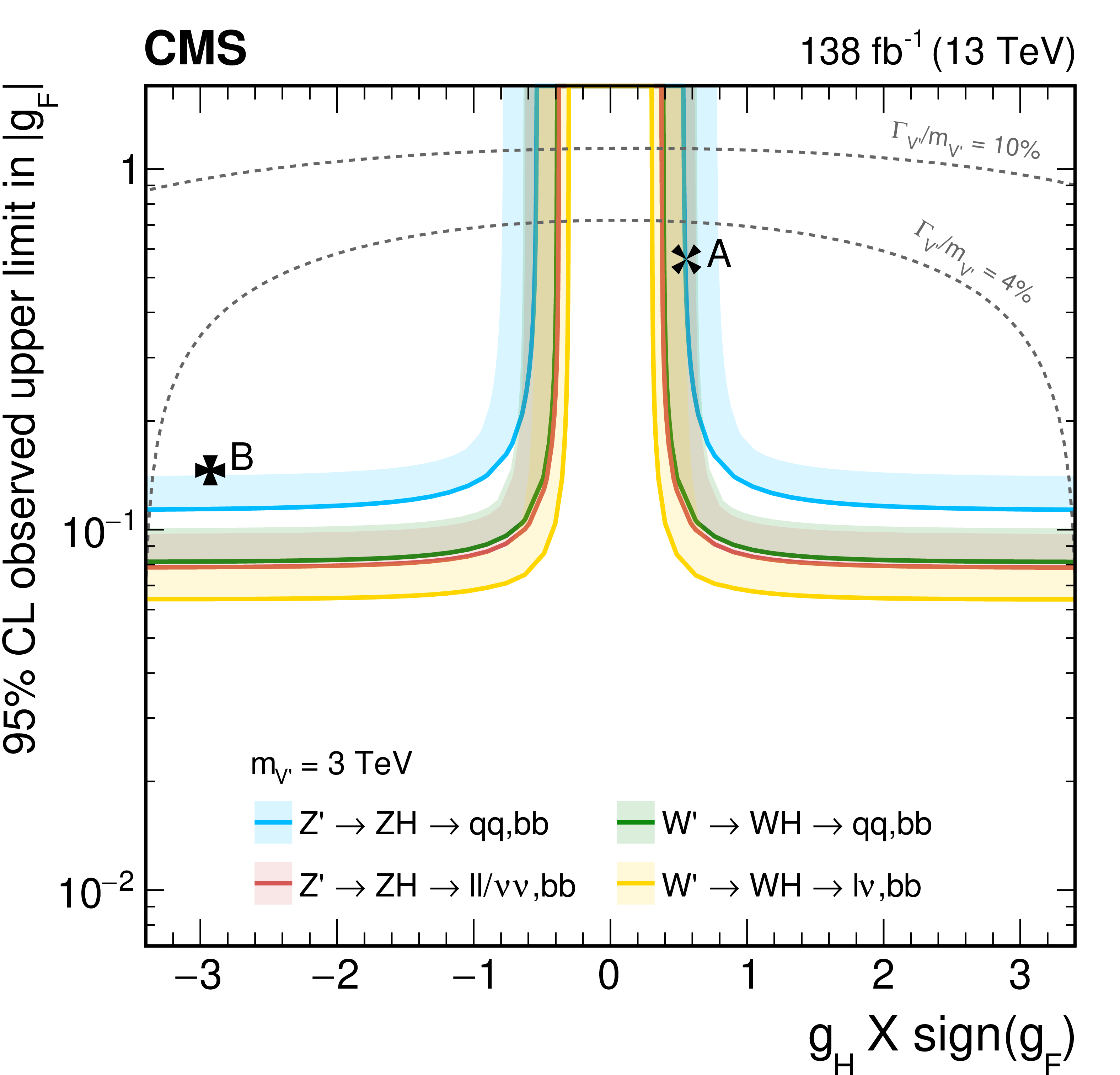
png pdf	Figure 38-c: Observed upper limits, at 95% CL, on the $ \mathrm{V}^{\prime} $ couplings $ g_\mathrm{F} $ and $ g_{\mathrm{H}} $ within the HVT model for $ \mathrm{V}^{\prime} $ masses of (upper left) 1, (upper right) 2, (lower left) 3, and (lower right) 4 TeV, from DY production, derived from VH channels of Refs. [109,110,111] discussed in this report. Excluded areas are indicated by the direction of the shading along the exclusion contours. The dotted lines denote coupling values above which the relative width of the resonance, $ \Gamma_{\mathrm{V}^{\prime}} /m_{V^{\prime}} $, exceeds 4 and 10%, respectively, implying that the narrow width approximation no longer applies. The couplings corresponding to the heavy vector triplet models A and B are indicated by cross markers.
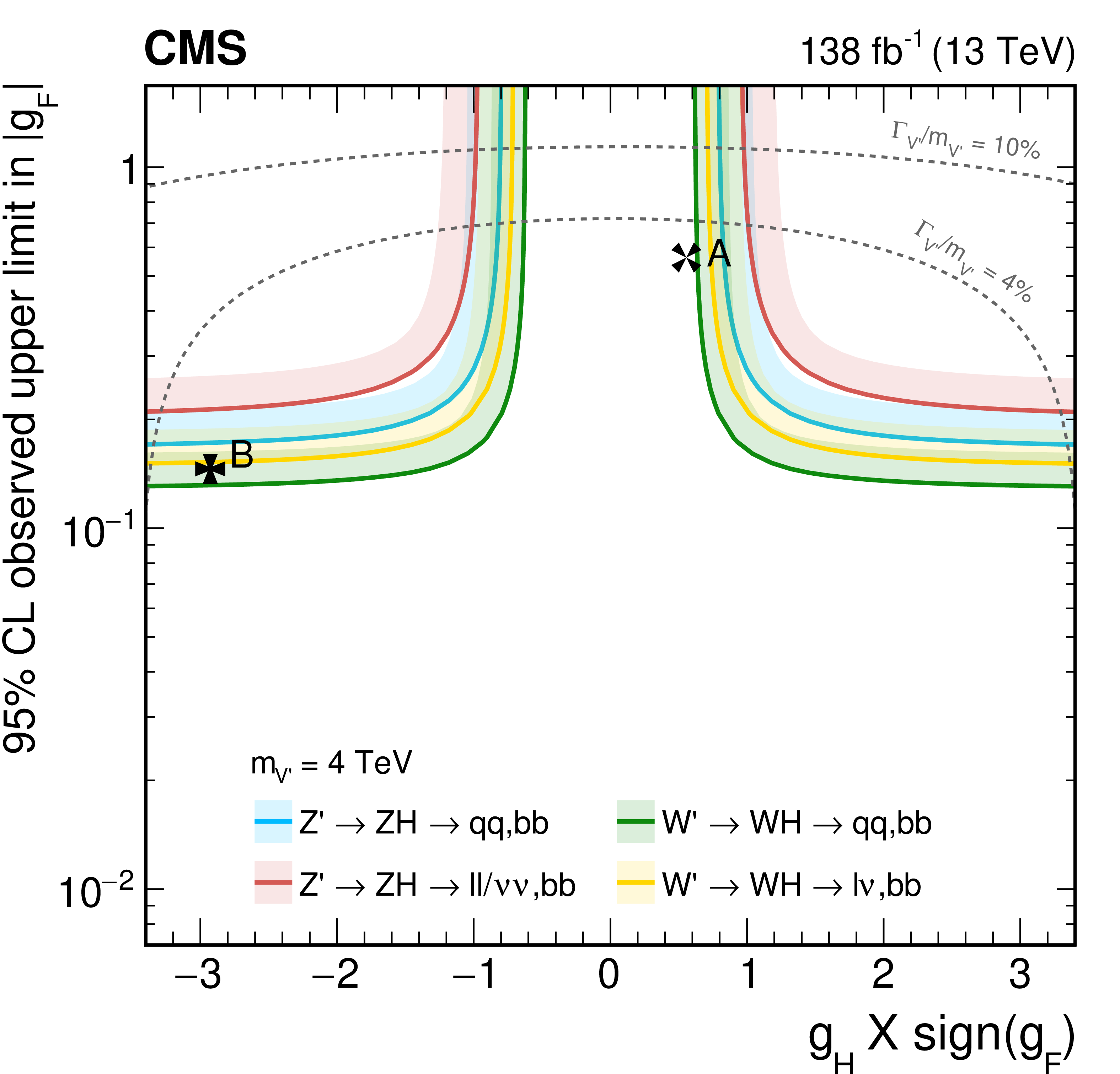
png pdf	Figure 38-d: Observed upper limits, at 95% CL, on the $ \mathrm{V}^{\prime} $ couplings $ g_\mathrm{F} $ and $ g_{\mathrm{H}} $ within the HVT model for $ \mathrm{V}^{\prime} $ masses of (upper left) 1, (upper right) 2, (lower left) 3, and (lower right) 4 TeV, from DY production, derived from VH channels of Refs. [109,110,111] discussed in this report. Excluded areas are indicated by the direction of the shading along the exclusion contours. The dotted lines denote coupling values above which the relative width of the resonance, $ \Gamma_{\mathrm{V}^{\prime}} /m_{V^{\prime}} $, exceeds 4 and 10%, respectively, implying that the narrow width approximation no longer applies. The couplings corresponding to the heavy vector triplet models A and B are indicated by cross markers.
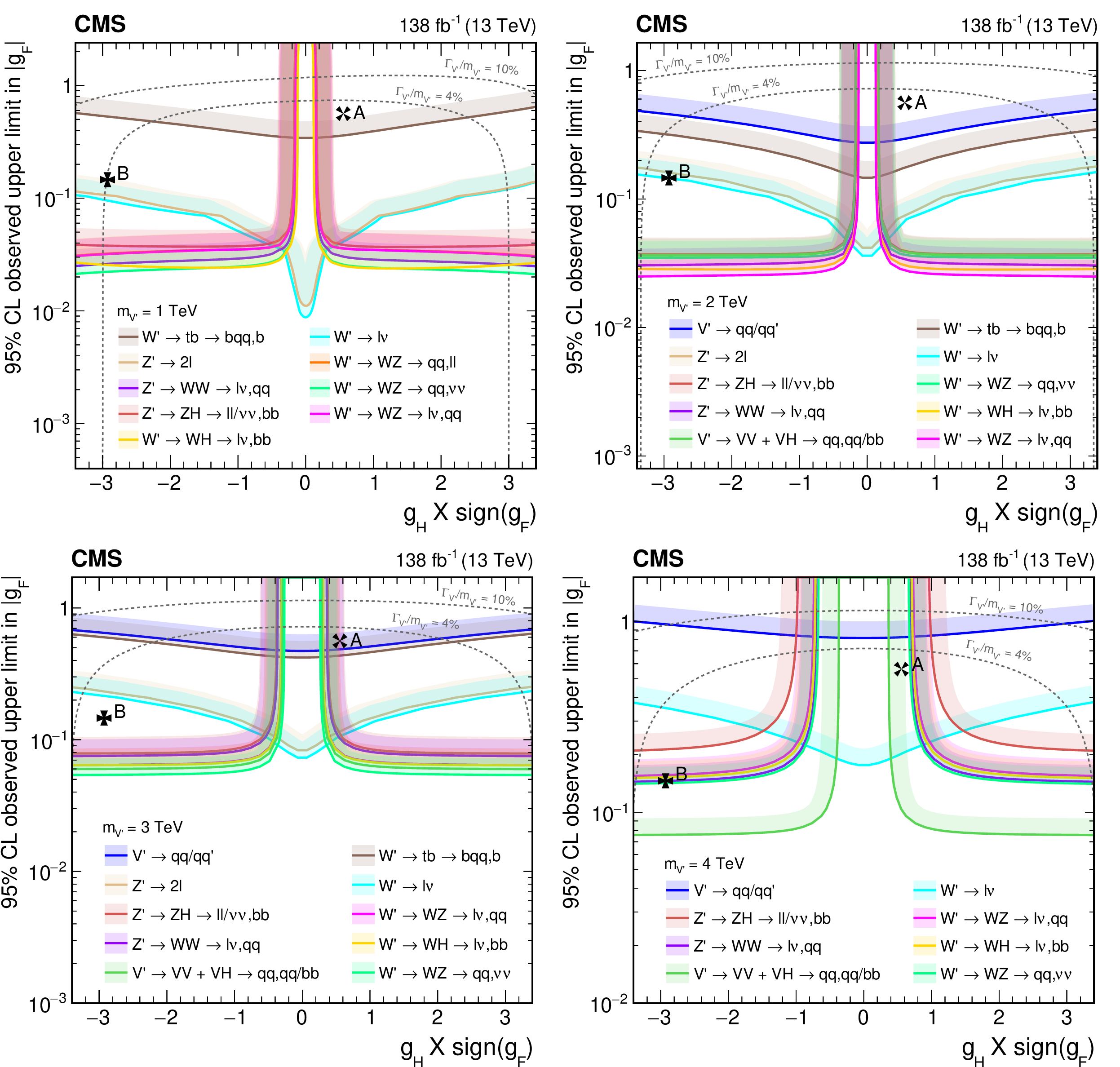
png pdf	Figure 39: Observed upper limits, at 95% CL, on the $ \mathrm{V}^{\prime} $ couplings $ g_\mathrm{F} $ and $ g_{\mathrm{H}} $ within the HVT model for $ \mathrm{V}^{\prime} $ masses of (upper left) 1, (upper right) 2, (lower left) 3, and (lower right) 4 TeV, from DY production, derived from VH channels of Refs. [109,110,111] discussed in this report and the VV channels of Refs.[109,111,197,196], as well as results from dijet [201], $ \mathrm{t}\mathrm{b} $ [199], as well as results from dijet [201], $ \mathrm{t}\mathrm{b} $ [199], $ \ell\ell $ [198] and $ \ell\nu $ [200] final states. Excluded areas are indicated by the direction of the shading along the exclusion contours. The dotted lines denote coupling values above which the relative width of the resonance, $ \Gamma_{\mathrm{V}^{\prime}}/m_{V^{\prime}} $, exceeds 4 and 10%, respectively, implying that the narrow width approximation no longer applies. The couplings corresponding to the heavy vector triplet models A and B are indicated by cross markers.
png pdf	Figure 39-a: Observed upper limits, at 95% CL, on the $ \mathrm{V}^{\prime} $ couplings $ g_\mathrm{F} $ and $ g_{\mathrm{H}} $ within the HVT model for $ \mathrm{V}^{\prime} $ masses of (upper left) 1, (upper right) 2, (lower left) 3, and (lower right) 4 TeV, from DY production, derived from VH channels of Refs. [109,110,111] discussed in this report and the VV channels of Refs.[109,111,197,196], as well as results from dijet [201], $ \mathrm{t}\mathrm{b} $ [199], as well as results from dijet [201], $ \mathrm{t}\mathrm{b} $ [199], $ \ell\ell $ [198] and $ \ell\nu $ [200] final states. Excluded areas are indicated by the direction of the shading along the exclusion contours. The dotted lines denote coupling values above which the relative width of the resonance, $ \Gamma_{\mathrm{V}^{\prime}}/m_{V^{\prime}} $, exceeds 4 and 10%, respectively, implying that the narrow width approximation no longer applies. The couplings corresponding to the heavy vector triplet models A and B are indicated by cross markers.
png pdf	Figure 39-b: Observed upper limits, at 95% CL, on the $ \mathrm{V}^{\prime} $ couplings $ g_\mathrm{F} $ and $ g_{\mathrm{H}} $ within the HVT model for $ \mathrm{V}^{\prime} $ masses of (upper left) 1, (upper right) 2, (lower left) 3, and (lower right) 4 TeV, from DY production, derived from VH channels of Refs. [109,110,111] discussed in this report and the VV channels of Refs.[109,111,197,196], as well as results from dijet [201], $ \mathrm{t}\mathrm{b} $ [199], as well as results from dijet [201], $ \mathrm{t}\mathrm{b} $ [199], $ \ell\ell $ [198] and $ \ell\nu $ [200] final states. Excluded areas are indicated by the direction of the shading along the exclusion contours. The dotted lines denote coupling values above which the relative width of the resonance, $ \Gamma_{\mathrm{V}^{\prime}}/m_{V^{\prime}} $, exceeds 4 and 10%, respectively, implying that the narrow width approximation no longer applies. The couplings corresponding to the heavy vector triplet models A and B are indicated by cross markers.
png pdf	Figure 39-c: Observed upper limits, at 95% CL, on the $ \mathrm{V}^{\prime} $ couplings $ g_\mathrm{F} $ and $ g_{\mathrm{H}} $ within the HVT model for $ \mathrm{V}^{\prime} $ masses of (upper left) 1, (upper right) 2, (lower left) 3, and (lower right) 4 TeV, from DY production, derived from VH channels of Refs. [109,110,111] discussed in this report and the VV channels of Refs.[109,111,197,196], as well as results from dijet [201], $ \mathrm{t}\mathrm{b} $ [199], as well as results from dijet [201], $ \mathrm{t}\mathrm{b} $ [199], $ \ell\ell $ [198] and $ \ell\nu $ [200] final states. Excluded areas are indicated by the direction of the shading along the exclusion contours. The dotted lines denote coupling values above which the relative width of the resonance, $ \Gamma_{\mathrm{V}^{\prime}}/m_{V^{\prime}} $, exceeds 4 and 10%, respectively, implying that the narrow width approximation no longer applies. The couplings corresponding to the heavy vector triplet models A and B are indicated by cross markers.
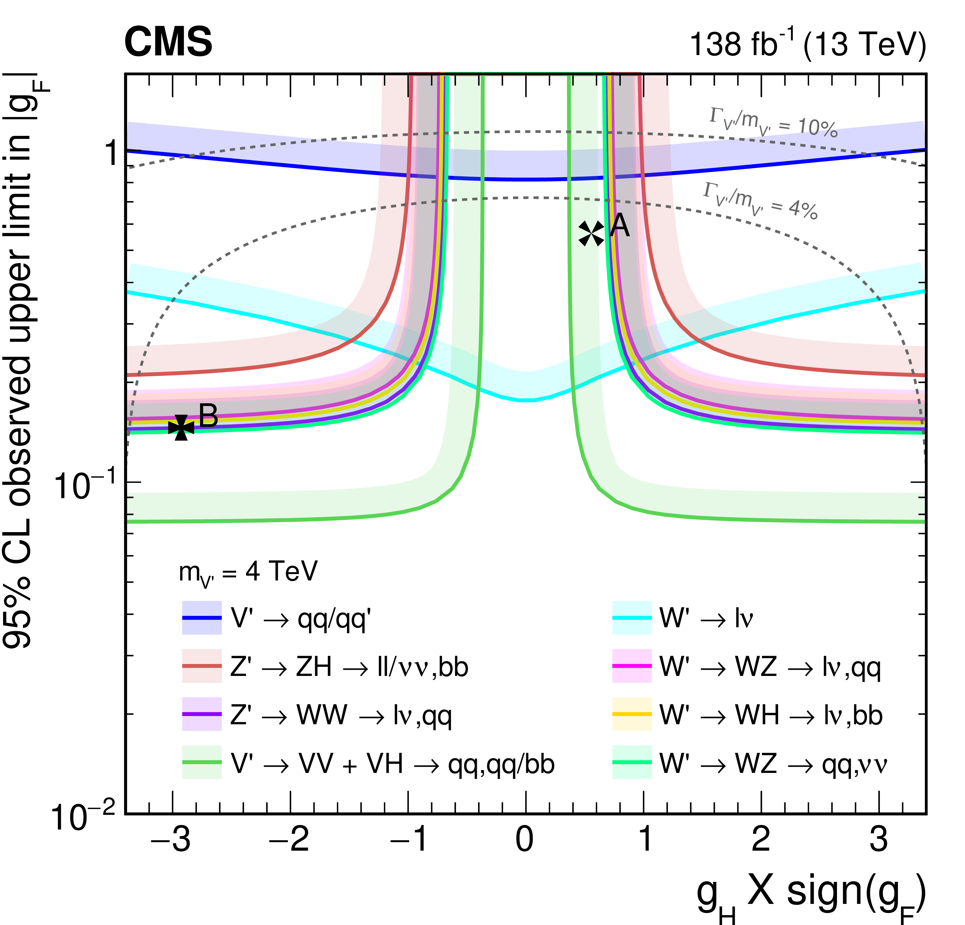
png pdf	Figure 39-d: Observed upper limits, at 95% CL, on the $ \mathrm{V}^{\prime} $ couplings $ g_\mathrm{F} $ and $ g_{\mathrm{H}} $ within the HVT model for $ \mathrm{V}^{\prime} $ masses of (upper left) 1, (upper right) 2, (lower left) 3, and (lower right) 4 TeV, from DY production, derived from VH channels of Refs. [109,110,111] discussed in this report and the VV channels of Refs.[109,111,197,196], as well as results from dijet [201], $ \mathrm{t}\mathrm{b} $ [199], as well as results from dijet [201], $ \mathrm{t}\mathrm{b} $ [199], $ \ell\ell $ [198] and $ \ell\nu $ [200] final states. Excluded areas are indicated by the direction of the shading along the exclusion contours. The dotted lines denote coupling values above which the relative width of the resonance, $ \Gamma_{\mathrm{V}^{\prime}}/m_{V^{\prime}} $, exceeds 4 and 10%, respectively, implying that the narrow width approximation no longer applies. The couplings corresponding to the heavy vector triplet models A and B are indicated by cross markers.
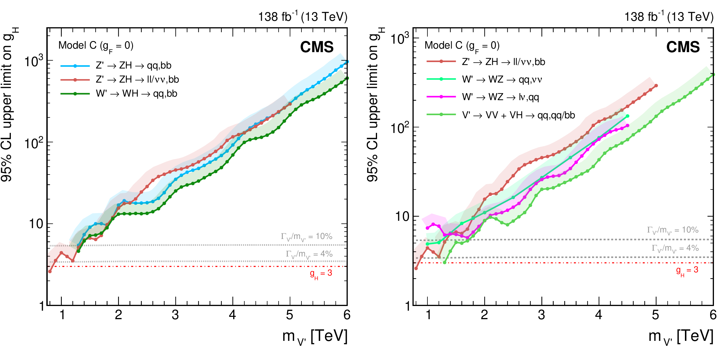
png pdf	Figure 40: Obseved upper limits, at 95% CL, on the coupling $ g_{\mathrm{H}} $ within the heavy vector triplet model, as a function of the $ \mathrm{V}^{\prime} $ mass. The limits are shown for the vecotr boson fusion production mode in the context of model C, in which $ g_\mathrm{F} = $ 0. The results are shown (left) for the WH and ZH analyses of Refs. [109,110,111], individually, and for a combination with the WZ final states of Refs. [196,111,109] (right), where the WH and ZH results from all-hadronic final states have been combined with the corresponding VV channels. The dotted lines denote coupling values above which the relative width of the resonance, $ \Gamma_{\mathrm{V}^{\prime}}/m_{V^{\prime}} $, exceeds 4 and 10%, respectively, implying the narrow width approximation no longer applies.
png pdf	Figure 40-a: Obseved upper limits, at 95% CL, on the coupling $ g_{\mathrm{H}} $ within the heavy vector triplet model, as a function of the $ \mathrm{V}^{\prime} $ mass. The limits are shown for the vecotr boson fusion production mode in the context of model C, in which $ g_\mathrm{F} = $ 0. The results are shown (left) for the WH and ZH analyses of Refs. [109,110,111], individually, and for a combination with the WZ final states of Refs. [196,111,109] (right), where the WH and ZH results from all-hadronic final states have been combined with the corresponding VV channels. The dotted lines denote coupling values above which the relative width of the resonance, $ \Gamma_{\mathrm{V}^{\prime}}/m_{V^{\prime}} $, exceeds 4 and 10%, respectively, implying the narrow width approximation no longer applies.
png pdf	Figure 40-b: Obseved upper limits, at 95% CL, on the coupling $ g_{\mathrm{H}} $ within the heavy vector triplet model, as a function of the $ \mathrm{V}^{\prime} $ mass. The limits are shown for the vecotr boson fusion production mode in the context of model C, in which $ g_\mathrm{F} = $ 0. The results are shown (left) for the WH and ZH analyses of Refs. [109,110,111], individually, and for a combination with the WZ final states of Refs. [196,111,109] (right), where the WH and ZH results from all-hadronic final states have been combined with the corresponding VV channels. The dotted lines denote coupling values above which the relative width of the resonance, $ \Gamma_{\mathrm{V}^{\prime}}/m_{V^{\prime}} $, exceeds 4 and 10%, respectively, implying the narrow width approximation no longer applies.
png pdf	Figure 41: Contours of the variable $ R_{\text{int}} $ as defined in Eq. (13) and discussed in the text, in the ($ \sin\alpha $, $ \lambda_{\mathrm{H}\mathrm{H}\mathrm{X}} $) plane for the singlet model with $ k_{\lambda} = $ 1 and different resonance masses $ m_{\mathrm{X}} $ between (upper left) 280 and (lower right) 800 GeV. Contours are shown for $ R_{\text{int}} $ values of (dashed blue) $-$0.2, (solid blue) $-$0.1, (solid green) $ + $0.1, and (dashed green) $ + $0.2. Regions that are excluded, at 95% CL, from the combined likelihood analysis of the HH analyses presented in this report are indicated by red filled areas. Dashed black lines indicate constant relative widths of 5, 10, and 20%.
png pdf	Figure 42: Expected differential cross sections for HH production, as a function of $ m_{{\mathrm{H}\mathrm{H}}} $, for the real-singlet model with $ m_{\mathrm{X}} = $ 280 GeV and $ \Gamma_{\mathrm{X}}/m_{\mathrm{X}} = 5% $. The parameters $ \sin\alpha $ and $ \lambda_{\mathrm{H}\mathrm{H}\mathrm{X}} $ have been chosen such that (upper row) $ R_{\text{int}}=\pm 10% $ and (lower row) $ R_{\text{int}}=\pm 20% $, for (left) negative and (right) positive values of $ R_{\text{int}} $. The total cross section for HH production $ \sigma^{\text{full}} $ (red line, labelled as $ \sigma_{\text{full}} $) is compared to the cross sections $ \sigma^{\text{ resonant-only}} $ (blue line, labelled as $ \sigma_{\text{res}} $) and $ \sigma^{ \text{nonresonant}} $ (green line, labelled as $ \sigma_{\text{nores}} $) considering only resonant and nonresonant production. In the lower panels the ratio of $ \sigma^{\text{full}} $ over $ (\sigma^{\text{resonant-only}}+\sigma^{ \text{nonresonant}}) $ is shown.
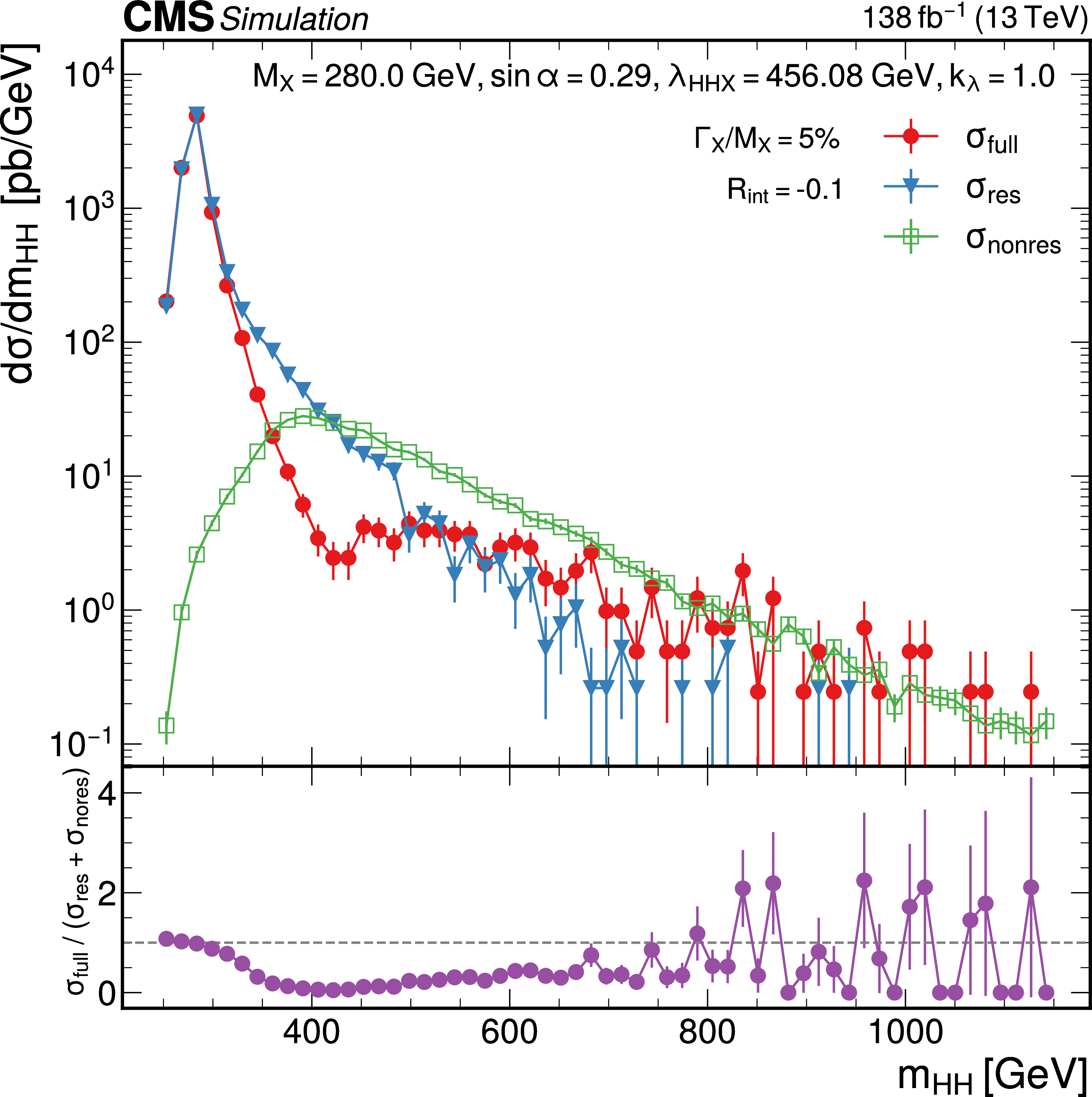
png pdf	Figure 42-a: Expected differential cross sections for HH production, as a function of $ m_{{\mathrm{H}\mathrm{H}}} $, for the real-singlet model with $ m_{\mathrm{X}} = $ 280 GeV and $ \Gamma_{\mathrm{X}}/m_{\mathrm{X}} = 5% $. The parameters $ \sin\alpha $ and $ \lambda_{\mathrm{H}\mathrm{H}\mathrm{X}} $ have been chosen such that (upper row) $ R_{\text{int}}=\pm 10% $ and (lower row) $ R_{\text{int}}=\pm 20% $, for (left) negative and (right) positive values of $ R_{\text{int}} $. The total cross section for HH production $ \sigma^{\text{full}} $ (red line, labelled as $ \sigma_{\text{full}} $) is compared to the cross sections $ \sigma^{\text{ resonant-only}} $ (blue line, labelled as $ \sigma_{\text{res}} $) and $ \sigma^{ \text{nonresonant}} $ (green line, labelled as $ \sigma_{\text{nores}} $) considering only resonant and nonresonant production. In the lower panels the ratio of $ \sigma^{\text{full}} $ over $ (\sigma^{\text{resonant-only}}+\sigma^{ \text{nonresonant}}) $ is shown.
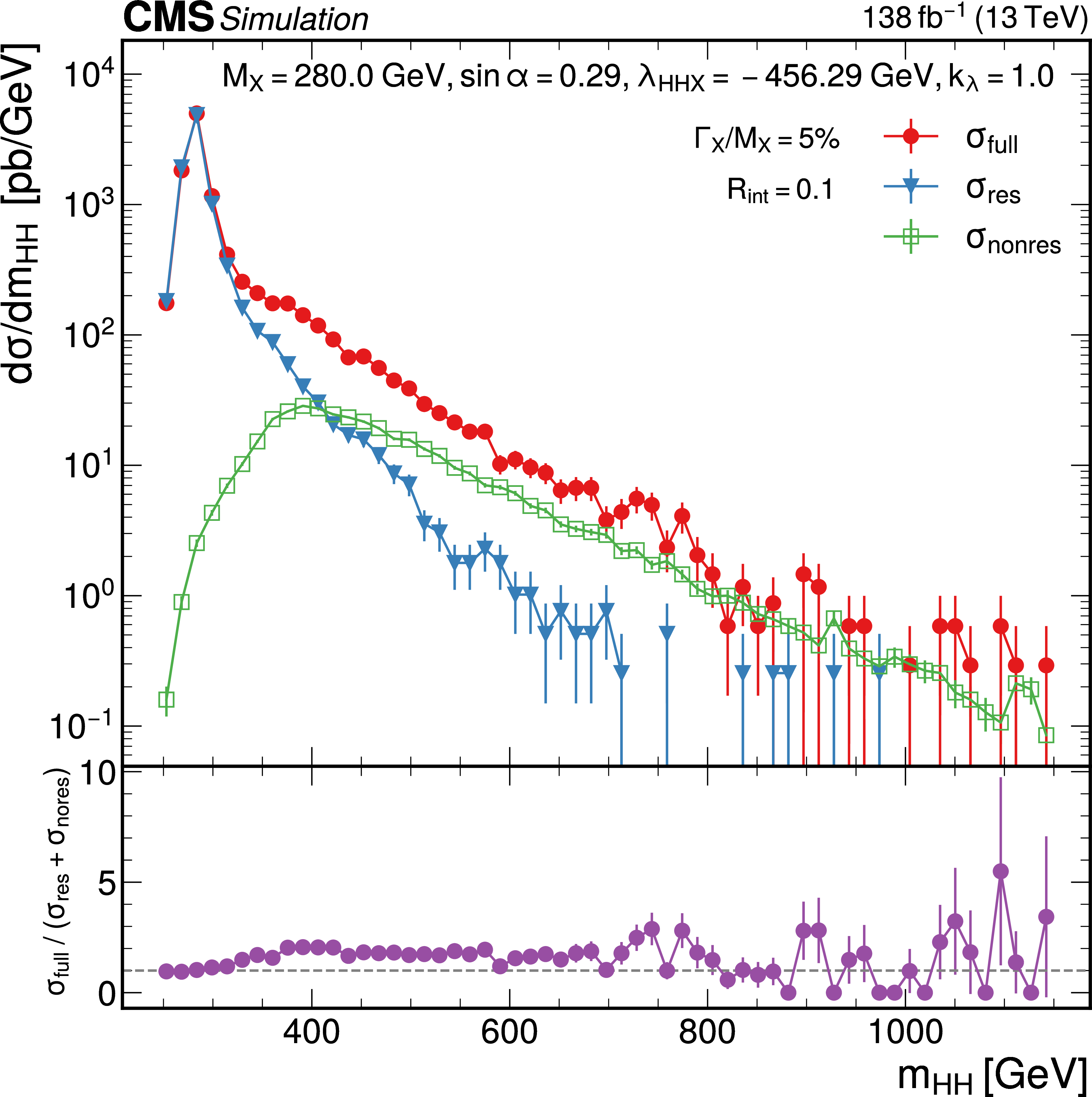
png pdf	Figure 42-b: Expected differential cross sections for HH production, as a function of $ m_{{\mathrm{H}\mathrm{H}}} $, for the real-singlet model with $ m_{\mathrm{X}} = $ 280 GeV and $ \Gamma_{\mathrm{X}}/m_{\mathrm{X}} = 5% $. The parameters $ \sin\alpha $ and $ \lambda_{\mathrm{H}\mathrm{H}\mathrm{X}} $ have been chosen such that (upper row) $ R_{\text{int}}=\pm 10% $ and (lower row) $ R_{\text{int}}=\pm 20% $, for (left) negative and (right) positive values of $ R_{\text{int}} $. The total cross section for HH production $ \sigma^{\text{full}} $ (red line, labelled as $ \sigma_{\text{full}} $) is compared to the cross sections $ \sigma^{\text{ resonant-only}} $ (blue line, labelled as $ \sigma_{\text{res}} $) and $ \sigma^{ \text{nonresonant}} $ (green line, labelled as $ \sigma_{\text{nores}} $) considering only resonant and nonresonant production. In the lower panels the ratio of $ \sigma^{\text{full}} $ over $ (\sigma^{\text{resonant-only}}+\sigma^{ \text{nonresonant}}) $ is shown.
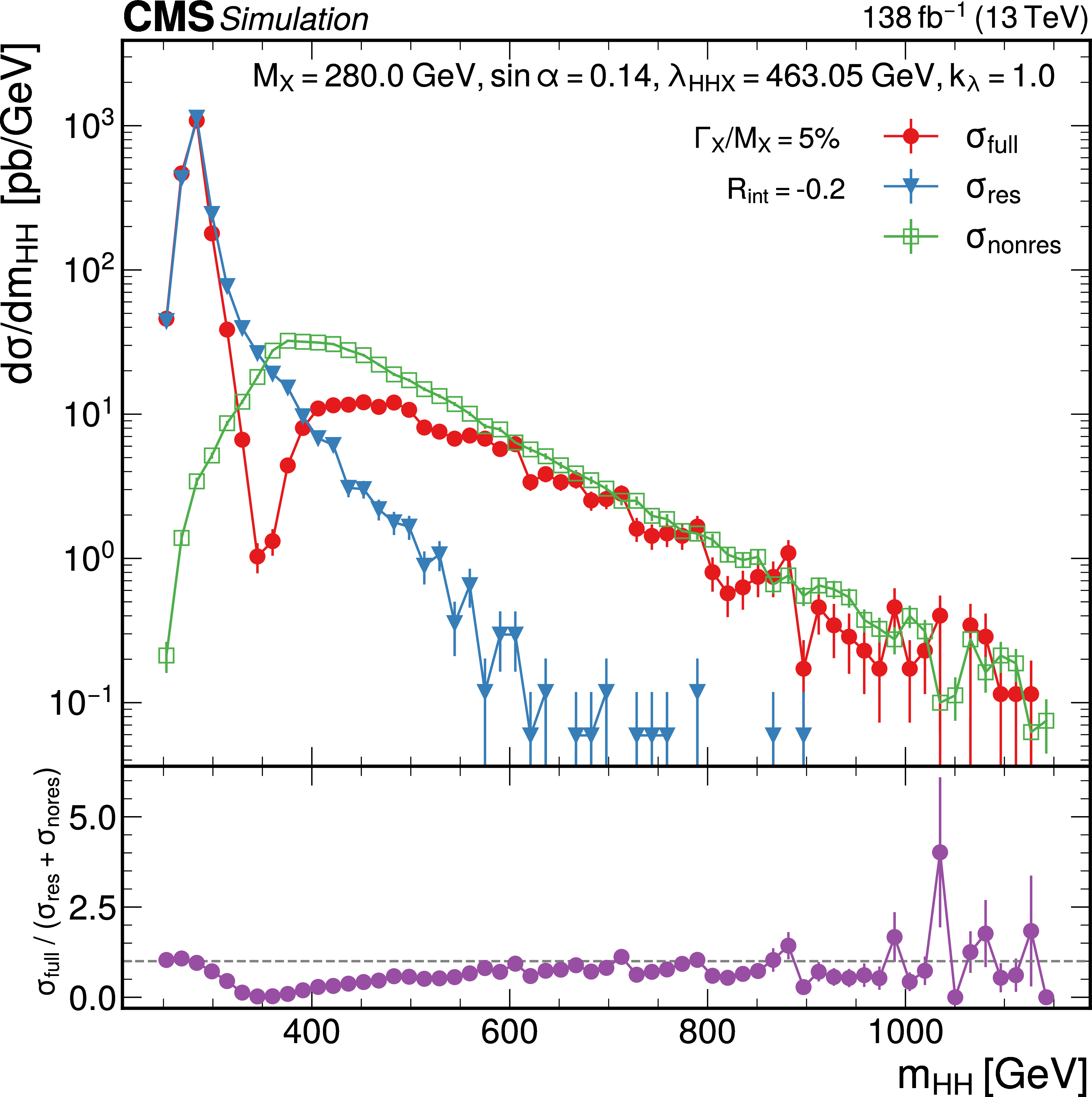
png pdf	Figure 42-c: Expected differential cross sections for HH production, as a function of $ m_{{\mathrm{H}\mathrm{H}}} $, for the real-singlet model with $ m_{\mathrm{X}} = $ 280 GeV and $ \Gamma_{\mathrm{X}}/m_{\mathrm{X}} = 5% $. The parameters $ \sin\alpha $ and $ \lambda_{\mathrm{H}\mathrm{H}\mathrm{X}} $ have been chosen such that (upper row) $ R_{\text{int}}=\pm 10% $ and (lower row) $ R_{\text{int}}=\pm 20% $, for (left) negative and (right) positive values of $ R_{\text{int}} $. The total cross section for HH production $ \sigma^{\text{full}} $ (red line, labelled as $ \sigma_{\text{full}} $) is compared to the cross sections $ \sigma^{\text{ resonant-only}} $ (blue line, labelled as $ \sigma_{\text{res}} $) and $ \sigma^{ \text{nonresonant}} $ (green line, labelled as $ \sigma_{\text{nores}} $) considering only resonant and nonresonant production. In the lower panels the ratio of $ \sigma^{\text{full}} $ over $ (\sigma^{\text{resonant-only}}+\sigma^{ \text{nonresonant}}) $ is shown.
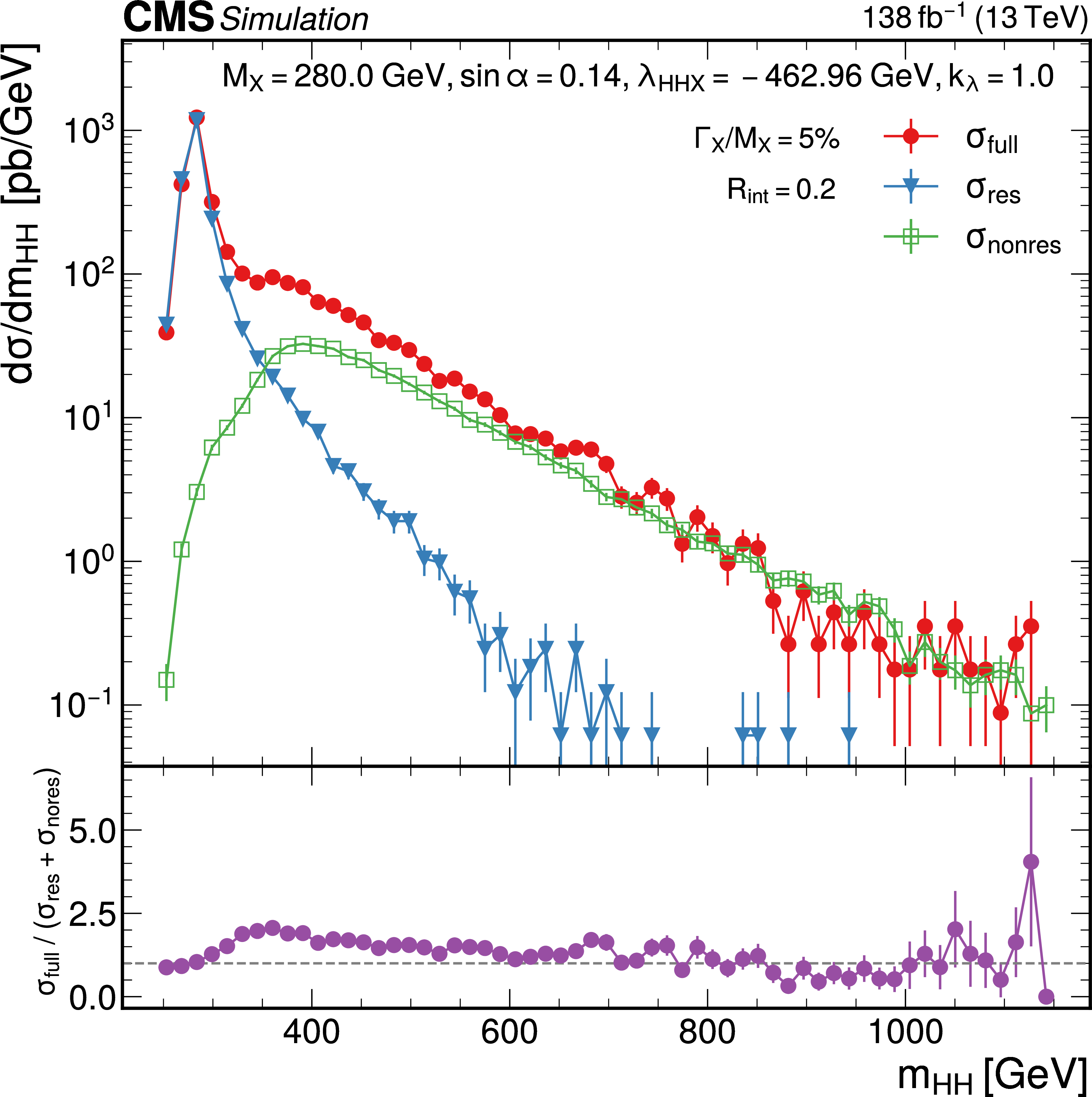
png pdf	Figure 42-d: Expected differential cross sections for HH production, as a function of $ m_{{\mathrm{H}\mathrm{H}}} $, for the real-singlet model with $ m_{\mathrm{X}} = $ 280 GeV and $ \Gamma_{\mathrm{X}}/m_{\mathrm{X}} = 5% $. The parameters $ \sin\alpha $ and $ \lambda_{\mathrm{H}\mathrm{H}\mathrm{X}} $ have been chosen such that (upper row) $ R_{\text{int}}=\pm 10% $ and (lower row) $ R_{\text{int}}=\pm 20% $, for (left) negative and (right) positive values of $ R_{\text{int}} $. The total cross section for HH production $ \sigma^{\text{full}} $ (red line, labelled as $ \sigma_{\text{full}} $) is compared to the cross sections $ \sigma^{\text{ resonant-only}} $ (blue line, labelled as $ \sigma_{\text{res}} $) and $ \sigma^{ \text{nonresonant}} $ (green line, labelled as $ \sigma_{\text{nores}} $) considering only resonant and nonresonant production. In the lower panels the ratio of $ \sigma^{\text{full}} $ over $ (\sigma^{\text{resonant-only}}+\sigma^{ \text{nonresonant}}) $ is shown.
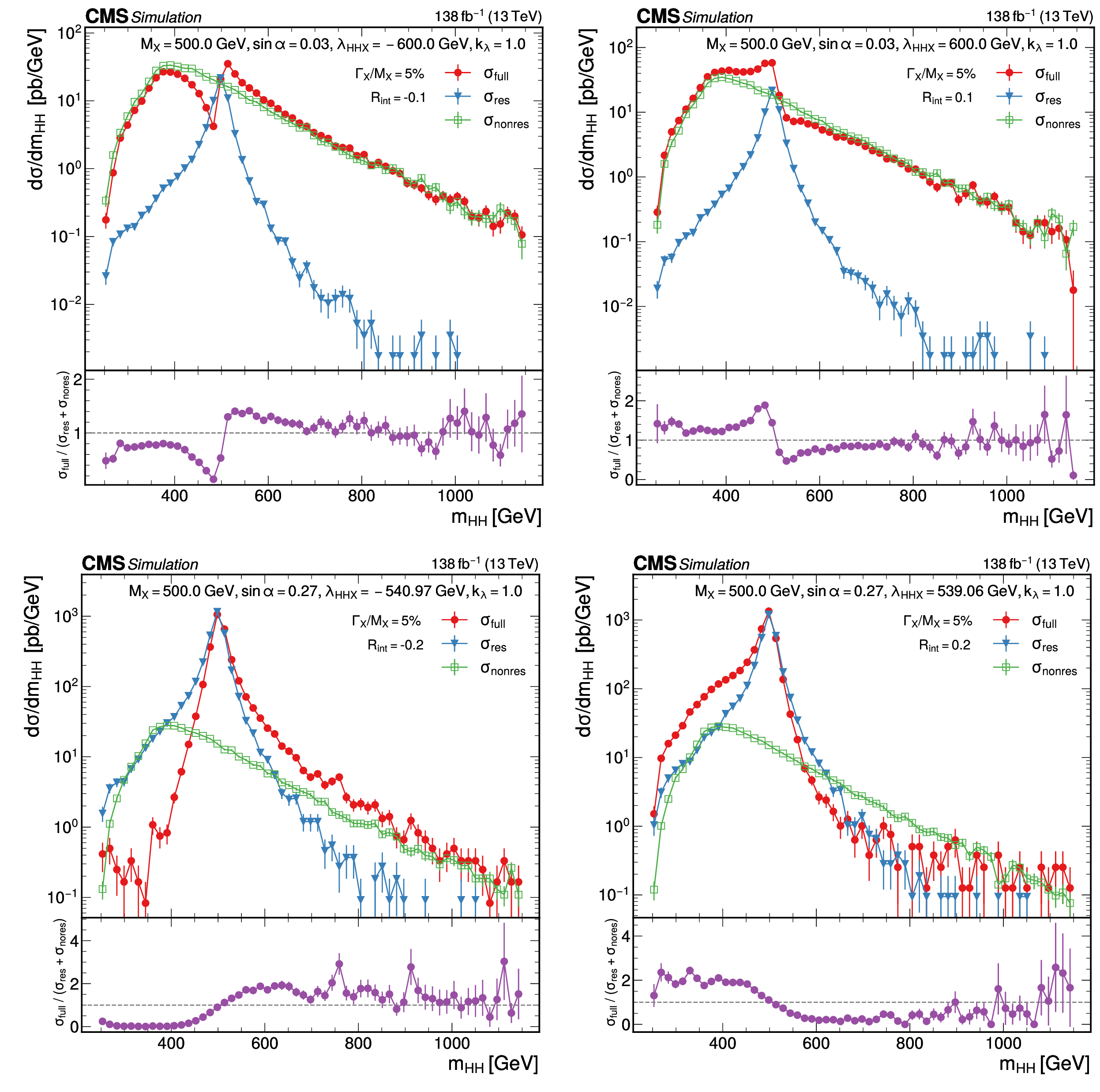
png pdf	Figure 43: Expected differential cross sections for HH production, as a function of $ m_{{\mathrm{H}\mathrm{H}}} $ for the real-singlet model with $ m_{\mathrm{X}} = $ 500 GeV and $ \Gamma_{\mathrm{X}}/m_{\mathrm{X}} = 5% $. The parameters $ \sin\alpha $ and $ \lambda_{\mathrm{H}\mathrm{H}\mathrm{X}} $ have been chosen such that (upper row) $ R_{\text{int}}=\pm 10% $ and (lower row) $ R_{\text{int}}=\pm 20% $, for (left) negative and (right) positive values of $ R_{\text{int}} $. The total cross section for HH production $ \sigma^{\text{full}} $ (red line, labelled as $ \sigma_{\text{full}} $) is compared to the cross sections $ \sigma^{\text{ resonant-only}} $ (blue line, labelled as $ \sigma_{\text{res}} $) and $ \sigma^{ \text{nonresonant}} $ (green line, labelled as $ \sigma_{\text{nores}} $) considering only resonant and nonresonant production. In the lower panels the ratio of $ \sigma^{\text{full}} $ over $ (\sigma^{\text{resonant-only}}+\sigma^{ \text{nonresonant}}) $ is shown.
png pdf	Figure 43-a: Expected differential cross sections for HH production, as a function of $ m_{{\mathrm{H}\mathrm{H}}} $ for the real-singlet model with $ m_{\mathrm{X}} = $ 500 GeV and $ \Gamma_{\mathrm{X}}/m_{\mathrm{X}} = 5% $. The parameters $ \sin\alpha $ and $ \lambda_{\mathrm{H}\mathrm{H}\mathrm{X}} $ have been chosen such that (upper row) $ R_{\text{int}}=\pm 10% $ and (lower row) $ R_{\text{int}}=\pm 20% $, for (left) negative and (right) positive values of $ R_{\text{int}} $. The total cross section for HH production $ \sigma^{\text{full}} $ (red line, labelled as $ \sigma_{\text{full}} $) is compared to the cross sections $ \sigma^{\text{ resonant-only}} $ (blue line, labelled as $ \sigma_{\text{res}} $) and $ \sigma^{ \text{nonresonant}} $ (green line, labelled as $ \sigma_{\text{nores}} $) considering only resonant and nonresonant production. In the lower panels the ratio of $ \sigma^{\text{full}} $ over $ (\sigma^{\text{resonant-only}}+\sigma^{ \text{nonresonant}}) $ is shown.
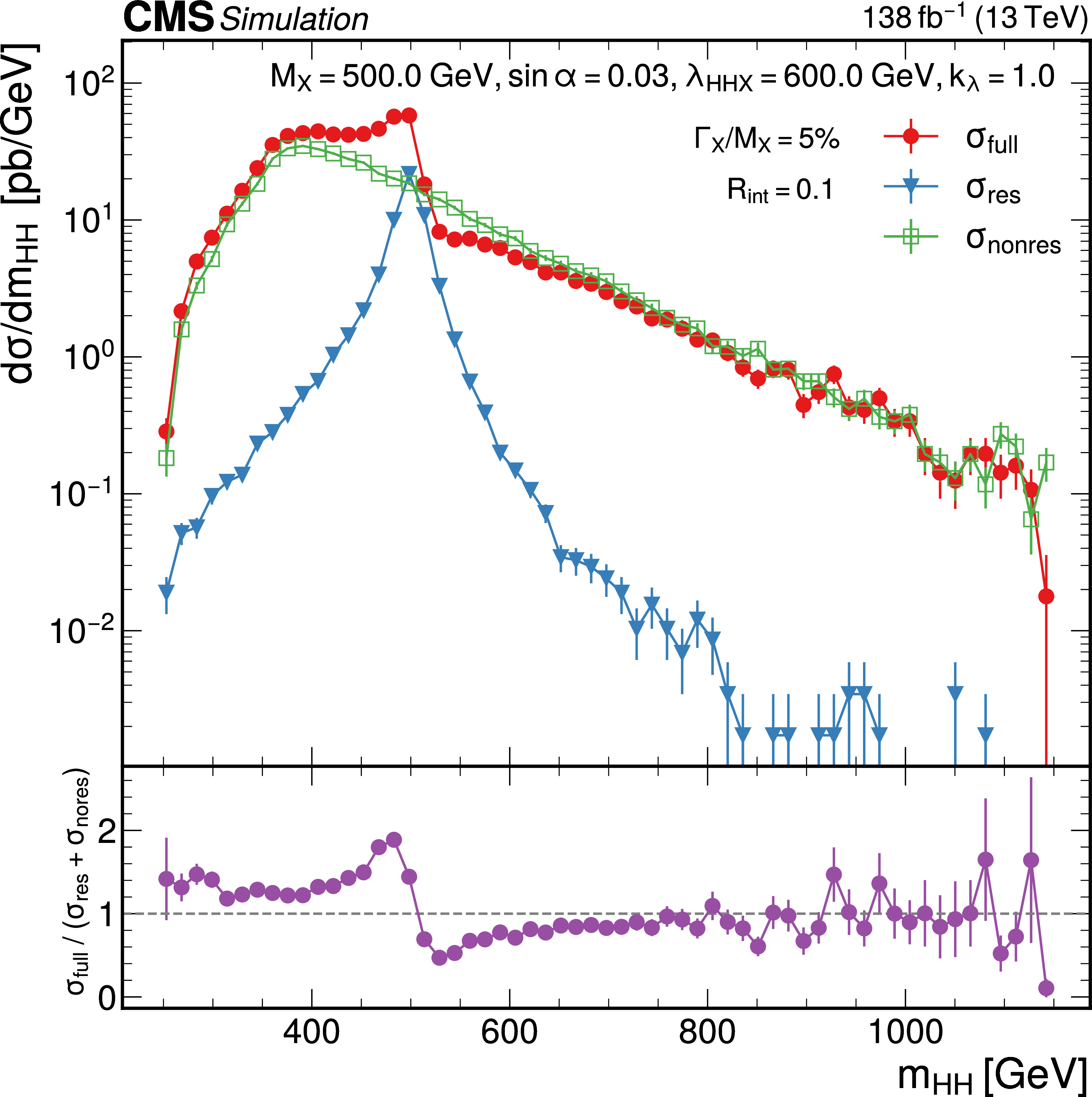
png pdf	Figure 43-b: Expected differential cross sections for HH production, as a function of $ m_{{\mathrm{H}\mathrm{H}}} $ for the real-singlet model with $ m_{\mathrm{X}} = $ 500 GeV and $ \Gamma_{\mathrm{X}}/m_{\mathrm{X}} = 5% $. The parameters $ \sin\alpha $ and $ \lambda_{\mathrm{H}\mathrm{H}\mathrm{X}} $ have been chosen such that (upper row) $ R_{\text{int}}=\pm 10% $ and (lower row) $ R_{\text{int}}=\pm 20% $, for (left) negative and (right) positive values of $ R_{\text{int}} $. The total cross section for HH production $ \sigma^{\text{full}} $ (red line, labelled as $ \sigma_{\text{full}} $) is compared to the cross sections $ \sigma^{\text{ resonant-only}} $ (blue line, labelled as $ \sigma_{\text{res}} $) and $ \sigma^{ \text{nonresonant}} $ (green line, labelled as $ \sigma_{\text{nores}} $) considering only resonant and nonresonant production. In the lower panels the ratio of $ \sigma^{\text{full}} $ over $ (\sigma^{\text{resonant-only}}+\sigma^{ \text{nonresonant}}) $ is shown.
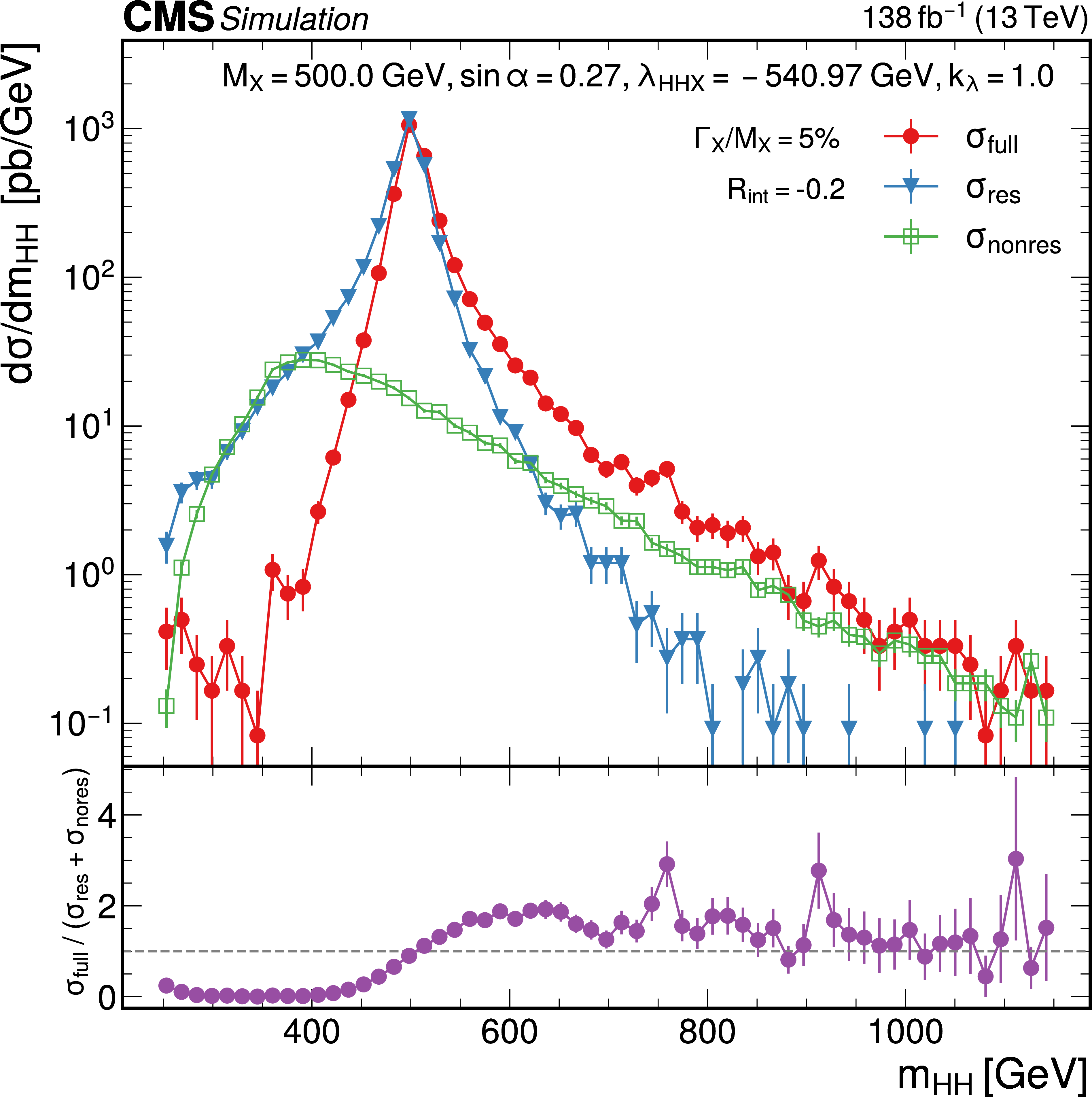
png pdf	Figure 43-c: Expected differential cross sections for HH production, as a function of $ m_{{\mathrm{H}\mathrm{H}}} $ for the real-singlet model with $ m_{\mathrm{X}} = $ 500 GeV and $ \Gamma_{\mathrm{X}}/m_{\mathrm{X}} = 5% $. The parameters $ \sin\alpha $ and $ \lambda_{\mathrm{H}\mathrm{H}\mathrm{X}} $ have been chosen such that (upper row) $ R_{\text{int}}=\pm 10% $ and (lower row) $ R_{\text{int}}=\pm 20% $, for (left) negative and (right) positive values of $ R_{\text{int}} $. The total cross section for HH production $ \sigma^{\text{full}} $ (red line, labelled as $ \sigma_{\text{full}} $) is compared to the cross sections $ \sigma^{\text{ resonant-only}} $ (blue line, labelled as $ \sigma_{\text{res}} $) and $ \sigma^{ \text{nonresonant}} $ (green line, labelled as $ \sigma_{\text{nores}} $) considering only resonant and nonresonant production. In the lower panels the ratio of $ \sigma^{\text{full}} $ over $ (\sigma^{\text{resonant-only}}+\sigma^{ \text{nonresonant}}) $ is shown.
png pdf	Figure 43-d: Expected differential cross sections for HH production, as a function of $ m_{{\mathrm{H}\mathrm{H}}} $ for the real-singlet model with $ m_{\mathrm{X}} = $ 500 GeV and $ \Gamma_{\mathrm{X}}/m_{\mathrm{X}} = 5% $. The parameters $ \sin\alpha $ and $ \lambda_{\mathrm{H}\mathrm{H}\mathrm{X}} $ have been chosen such that (upper row) $ R_{\text{int}}=\pm 10% $ and (lower row) $ R_{\text{int}}=\pm 20% $, for (left) negative and (right) positive values of $ R_{\text{int}} $. The total cross section for HH production $ \sigma^{\text{full}} $ (red line, labelled as $ \sigma_{\text{full}} $) is compared to the cross sections $ \sigma^{\text{ resonant-only}} $ (blue line, labelled as $ \sigma_{\text{res}} $) and $ \sigma^{ \text{nonresonant}} $ (green line, labelled as $ \sigma_{\text{nores}} $) considering only resonant and nonresonant production. In the lower panels the ratio of $ \sigma^{\text{full}} $ over $ (\sigma^{\text{resonant-only}}+\sigma^{ \text{nonresonant}}) $ is shown.
png pdf	Figure 44: Expected upper limits at 95% CL, on the product of the cross section for the production of a spin-0 resonance X and the branching fraction $ \mathcal{B}(\mathrm{X} \to\mathrm{H}\mathrm{H}) $, as functions of $ m_{\mathrm{X}} $ from the (upper left) $ \mathrm{b}\mathrm{b}\tau\tau $ [115], (upper right) $ \mathrm{b}\mathrm{b}\gamma\gamma $ [116], and (lower) $ \mathrm{b}\mathrm{b}\mathrm{b}\mathrm{b} $ with two merged $ \mathrm{b}\mathrm{b} $ jets [117] analyses discussed in this report, projected to an integrated luminosity of 3000 fb$ ^{-1} $ under the assumption of different systematic uncertainty scenarios, as discussed in the text. All estimates include the anticipated statistical uncertainties.
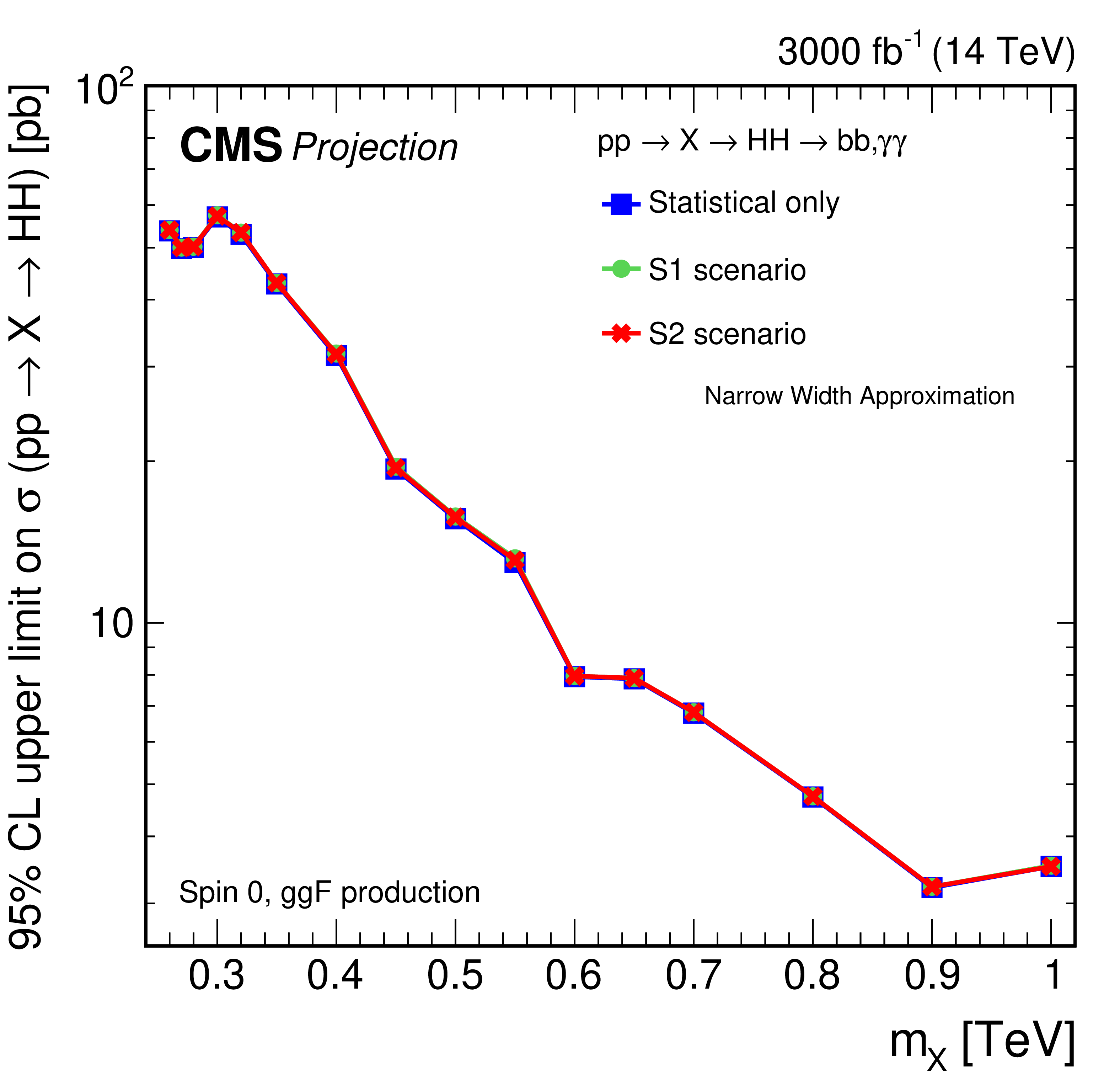
png pdf	Figure 44-a: Expected upper limits at 95% CL, on the product of the cross section for the production of a spin-0 resonance X and the branching fraction $ \mathcal{B}(\mathrm{X} \to\mathrm{H}\mathrm{H}) $, as functions of $ m_{\mathrm{X}} $ from the (upper left) $ \mathrm{b}\mathrm{b}\tau\tau $ [115], (upper right) $ \mathrm{b}\mathrm{b}\gamma\gamma $ [116], and (lower) $ \mathrm{b}\mathrm{b}\mathrm{b}\mathrm{b} $ with two merged $ \mathrm{b}\mathrm{b} $ jets [117] analyses discussed in this report, projected to an integrated luminosity of 3000 fb$ ^{-1} $ under the assumption of different systematic uncertainty scenarios, as discussed in the text. All estimates include the anticipated statistical uncertainties.
png pdf	Figure 44-b: Expected upper limits at 95% CL, on the product of the cross section for the production of a spin-0 resonance X and the branching fraction $ \mathcal{B}(\mathrm{X} \to\mathrm{H}\mathrm{H}) $, as functions of $ m_{\mathrm{X}} $ from the (upper left) $ \mathrm{b}\mathrm{b}\tau\tau $ [115], (upper right) $ \mathrm{b}\mathrm{b}\gamma\gamma $ [116], and (lower) $ \mathrm{b}\mathrm{b}\mathrm{b}\mathrm{b} $ with two merged $ \mathrm{b}\mathrm{b} $ jets [117] analyses discussed in this report, projected to an integrated luminosity of 3000 fb$ ^{-1} $ under the assumption of different systematic uncertainty scenarios, as discussed in the text. All estimates include the anticipated statistical uncertainties.
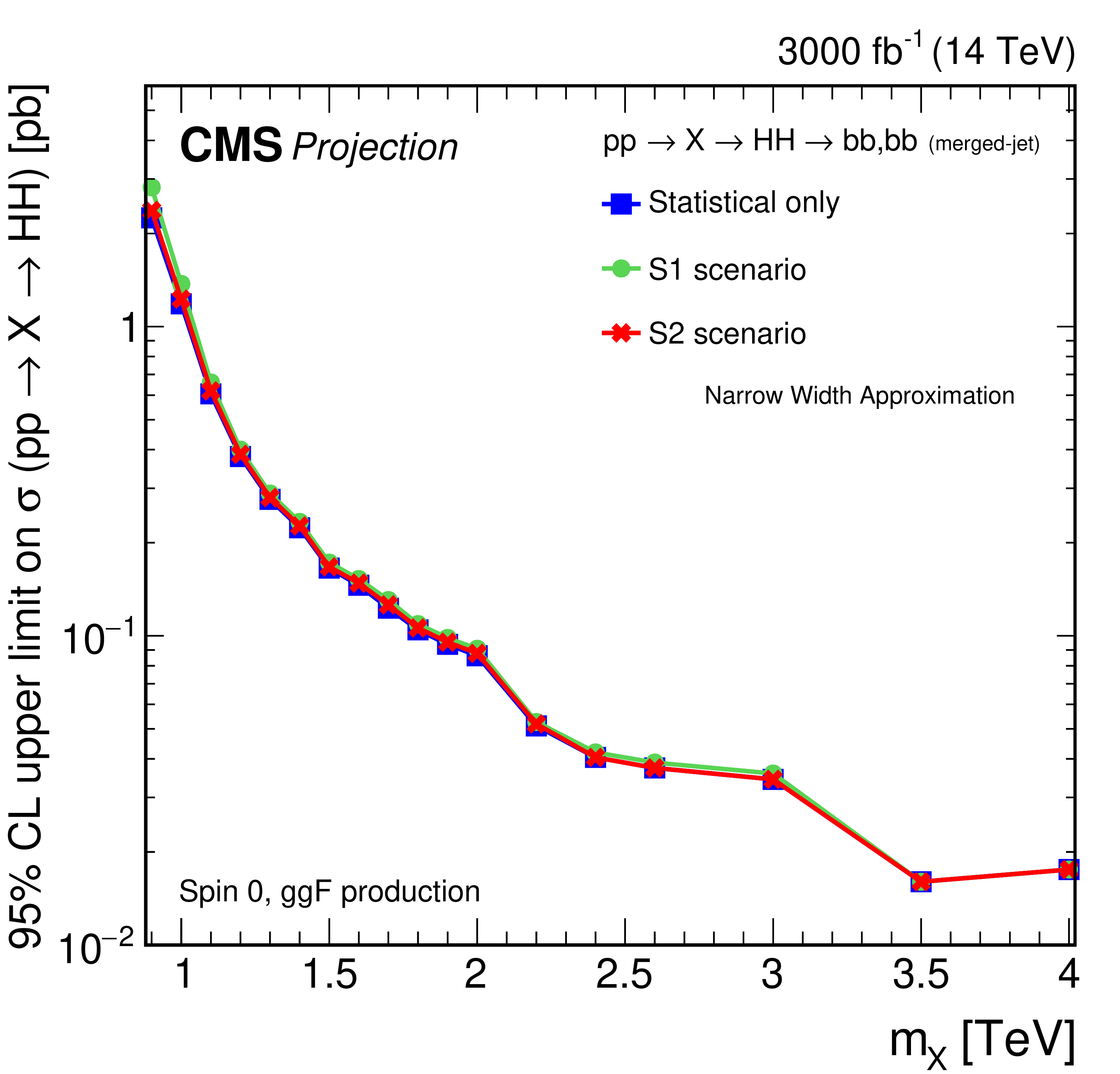
png pdf	Figure 44-c: Expected upper limits at 95% CL, on the product of the cross section for the production of a spin-0 resonance X and the branching fraction $ \mathcal{B}(\mathrm{X} \to\mathrm{H}\mathrm{H}) $, as functions of $ m_{\mathrm{X}} $ from the (upper left) $ \mathrm{b}\mathrm{b}\tau\tau $ [115], (upper right) $ \mathrm{b}\mathrm{b}\gamma\gamma $ [116], and (lower) $ \mathrm{b}\mathrm{b}\mathrm{b}\mathrm{b} $ with two merged $ \mathrm{b}\mathrm{b} $ jets [117] analyses discussed in this report, projected to an integrated luminosity of 3000 fb$ ^{-1} $ under the assumption of different systematic uncertainty scenarios, as discussed in the text. All estimates include the anticipated statistical uncertainties.
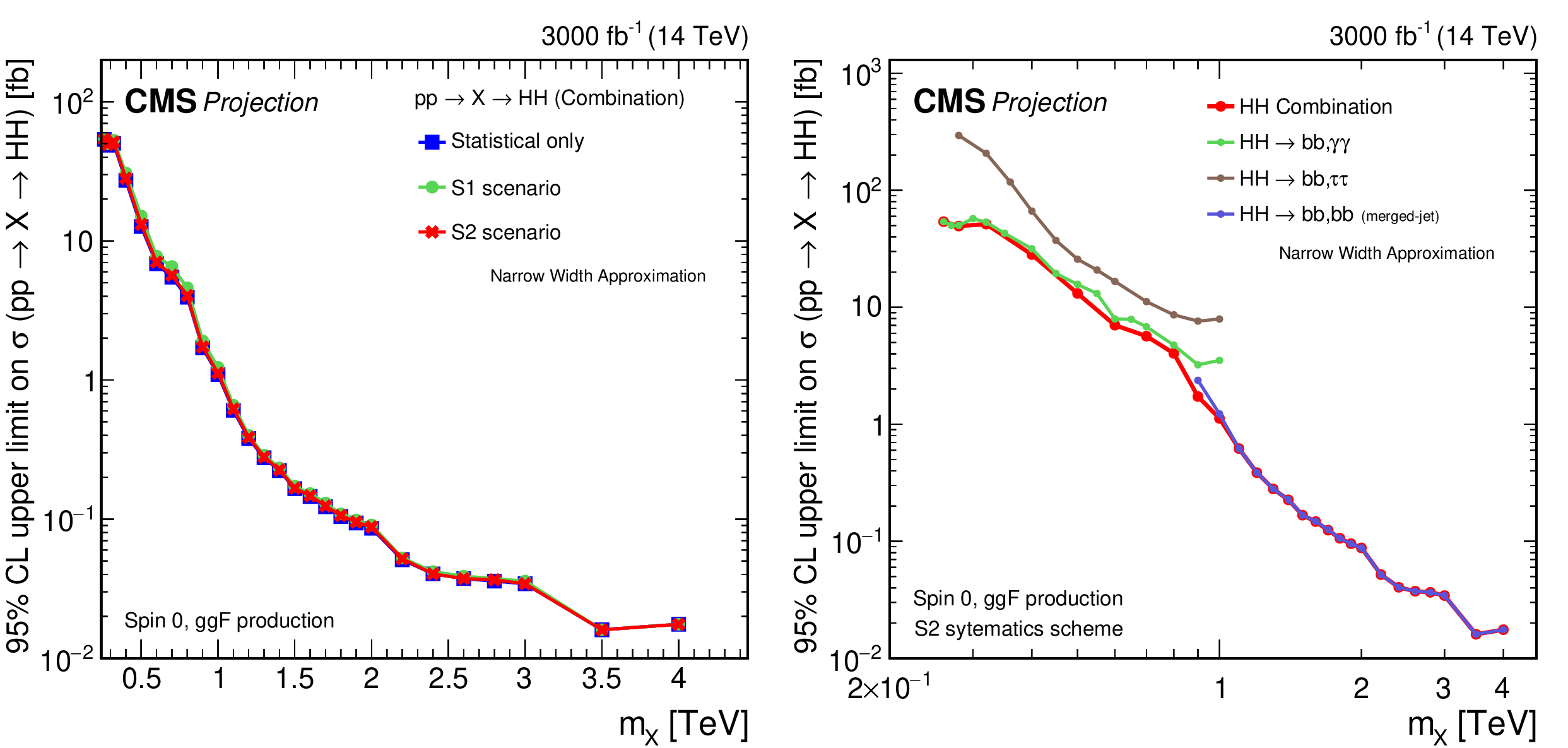
png pdf	Figure 45: Expected upper limits at 95% CL, on the product of the cross section for the production of a spin-0 resonance X and the branching fraction $ \mathcal{B}(\mathrm{X} \to\mathrm{H}\mathrm{H}) $, as a function of $ m_{\mathrm{X}} $, for an integrated luminosity of 3000 fb$ ^{-1} $ and the combination of the three analyses shown in Fig. 44. Shown are the effects of the different systematic uncertainty scenarios (left), and the reach of the individual analyses for the S2 systematic scenario (right). All estimates include the anticipated statistical uncertainties.
png pdf	Figure 45-a: Expected upper limits at 95% CL, on the product of the cross section for the production of a spin-0 resonance X and the branching fraction $ \mathcal{B}(\mathrm{X} \to\mathrm{H}\mathrm{H}) $, as a function of $ m_{\mathrm{X}} $, for an integrated luminosity of 3000 fb$ ^{-1} $ and the combination of the three analyses shown in Fig. 44. Shown are the effects of the different systematic uncertainty scenarios (left), and the reach of the individual analyses for the S2 systematic scenario (right). All estimates include the anticipated statistical uncertainties.
png pdf	Figure 45-b: Expected upper limits at 95% CL, on the product of the cross section for the production of a spin-0 resonance X and the branching fraction $ \mathcal{B}(\mathrm{X} \to\mathrm{H}\mathrm{H}) $, as a function of $ m_{\mathrm{X}} $, for an integrated luminosity of 3000 fb$ ^{-1} $ and the combination of the three analyses shown in Fig. 44. Shown are the effects of the different systematic uncertainty scenarios (left), and the reach of the individual analyses for the S2 systematic scenario (right). All estimates include the anticipated statistical uncertainties.
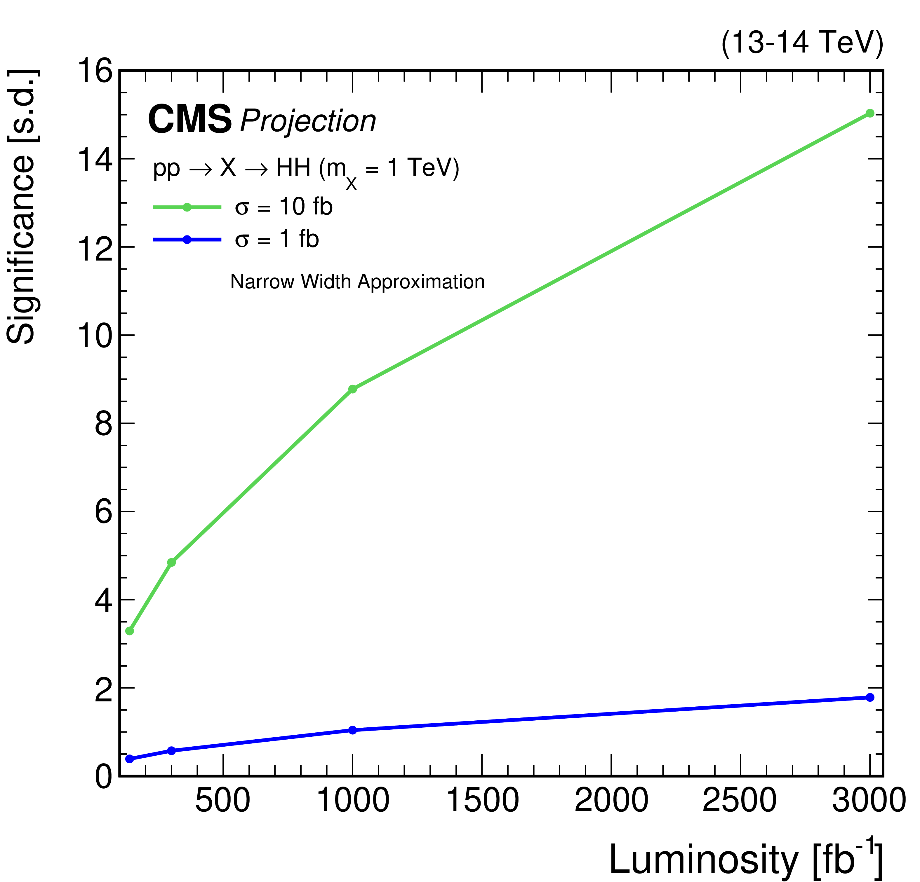
png pdf	Figure 46: Expected discovery significance for a spin-0 resonance X with $ m_{\mathrm{X}}= $ 1 TeV and cross sections of 1 and 10 fb, obtained for the combined likelihood analysis of the resonant HH searches as discussed in Section 5 and shown in Figs. 44 and 45, shown as function of the integrated luminosity.
png pdf	Figure 47: Expected exclusion contours at 95% CL, in the ($ \tan\beta $, $ m_{{\mathrm{A}}} $) plane of the (left) hMSSM and (right) $ M^{125}_{\text{h,EFT}} $ scenarios obtained from the combined likelihood analysis of the HH searches discussed in Section 4.1 and shown in Figs. 31 and 32, for different integrated luminosities and compared to the Run 2 result obtained at $ \sqrt{s}= $ 13 TeV. The projections assume $ \sqrt{s}= $ 14 TeV.
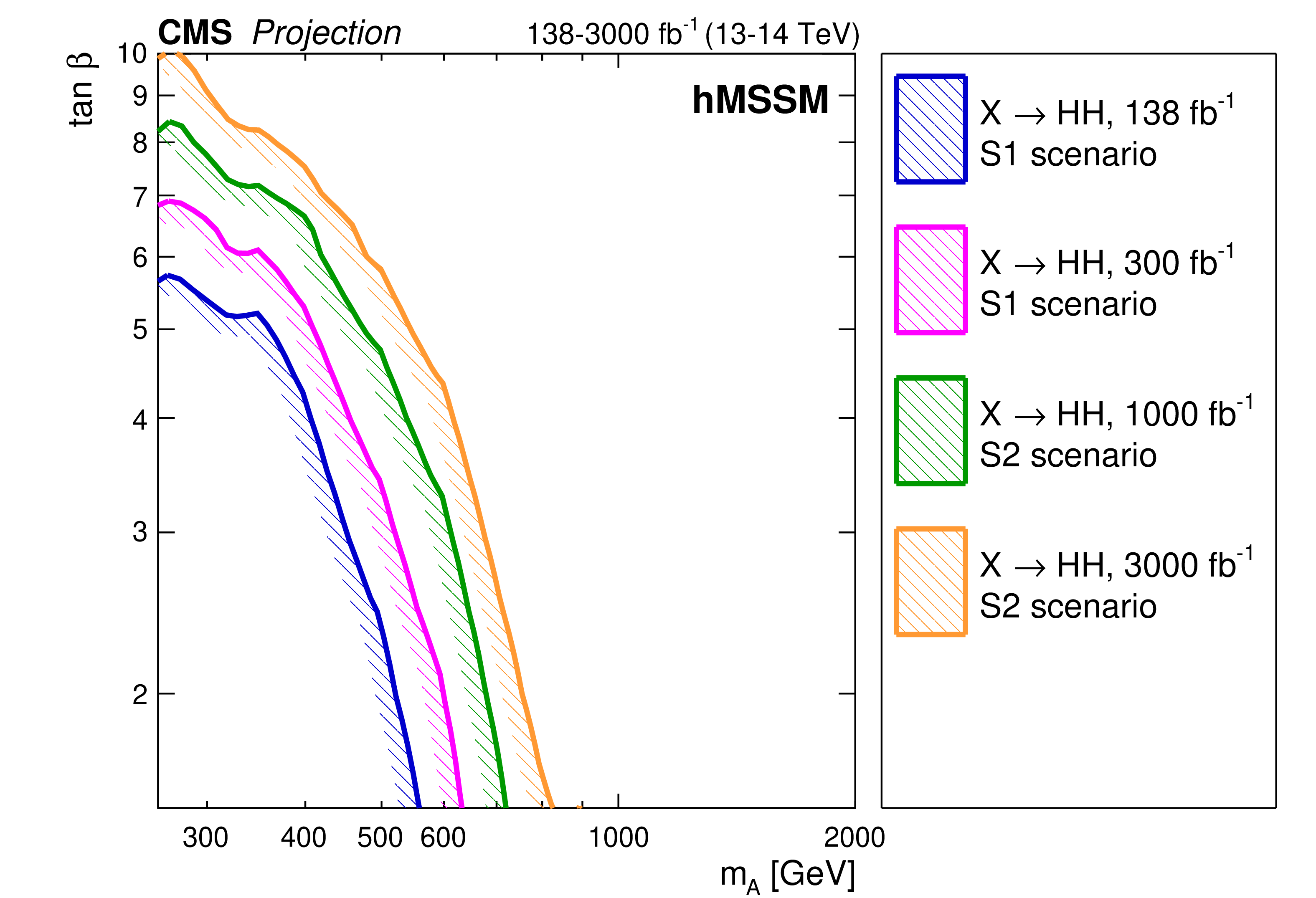
png pdf	Figure 47-a: Expected exclusion contours at 95% CL, in the ($ \tan\beta $, $ m_{{\mathrm{A}}} $) plane of the (left) hMSSM and (right) $ M^{125}_{\text{h,EFT}} $ scenarios obtained from the combined likelihood analysis of the HH searches discussed in Section 4.1 and shown in Figs. 31 and 32, for different integrated luminosities and compared to the Run 2 result obtained at $ \sqrt{s}= $ 13 TeV. The projections assume $ \sqrt{s}= $ 14 TeV.
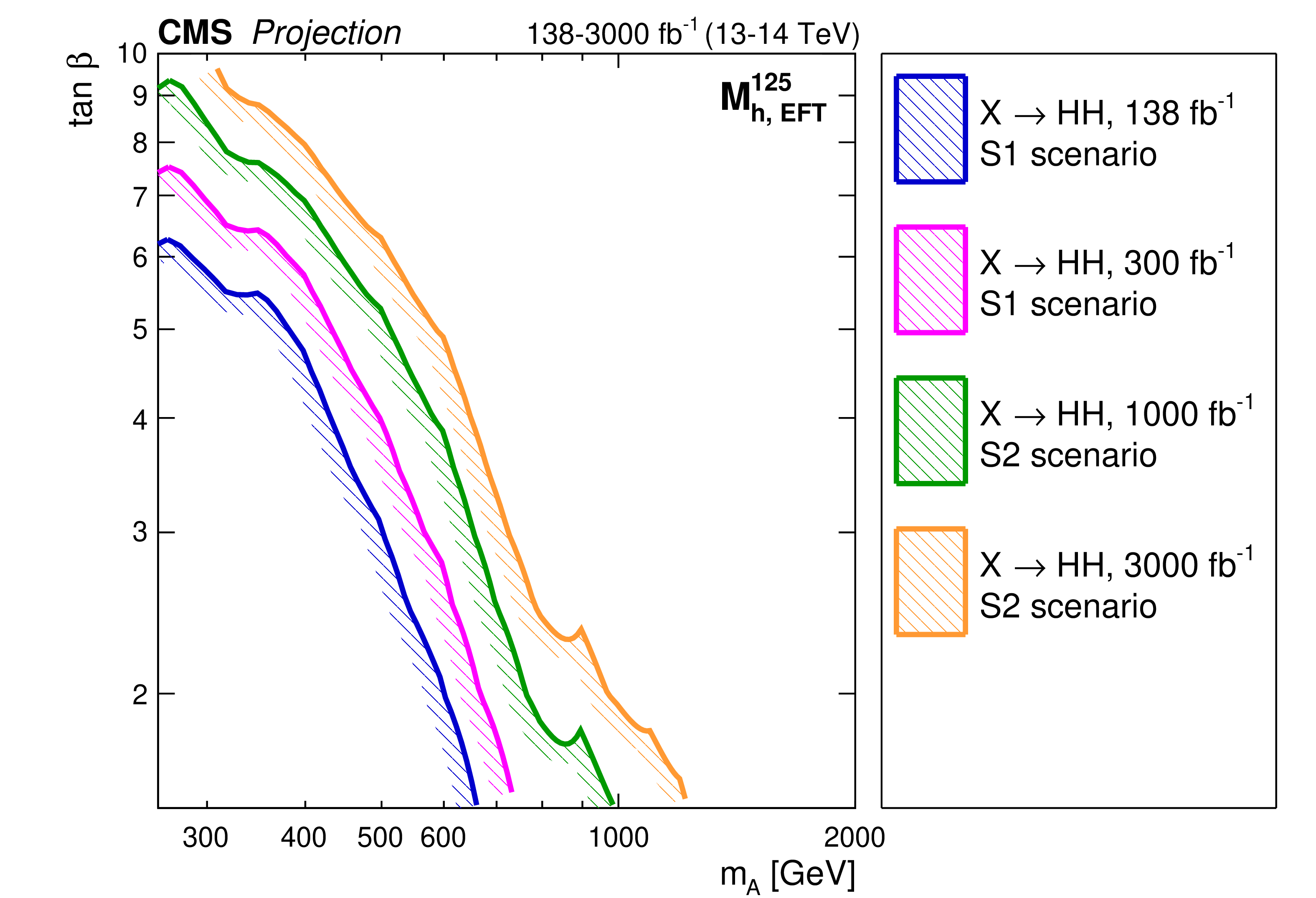
png pdf	Figure 47-b: Expected exclusion contours at 95% CL, in the ($ \tan\beta $, $ m_{{\mathrm{A}}} $) plane of the (left) hMSSM and (right) $ M^{125}_{\text{h,EFT}} $ scenarios obtained from the combined likelihood analysis of the HH searches discussed in Section 4.1 and shown in Figs. 31 and 32, for different integrated luminosities and compared to the Run 2 result obtained at $ \sqrt{s}= $ 13 TeV. The projections assume $ \sqrt{s}= $ 14 TeV.
png pdf	Figure 48: Expected lower limit at 95% CL, on $ \Lambda_{\mathrm{R}} $ in the warped extra dimensions bulk scenario for the production of a radion R, as a function of $ m_{{\mathrm{R}} } $. The limits are derived from the combined likelihood analysis of the HH searches discussed in Section 4.2 and shown in Fig. 35, for different values of the integrated luminosity. Excluded areas are indicated by the direction of the hatching along the exclusion contours.
png pdf	Figure 49: Exclusion contours at 95% CL, in the ($ \sin\alpha $, $ \lambda_{\mathrm{H}\mathrm{H}\mathrm{X}} $) plane for $ k_{\lambda} = $ 1 in the real-singlet model. These contours are obtained from the combined likelihood analysis of the HH searches discussed in Section 4.1 for (upper left to lower right) $ m_{\mathrm{X}} = $ 280, 400, 500, 600, 700, and 1000 GeV. The expected limits from the Run 2 dataset have been projected to integrated luminosities of 300, 1000, and 3000 fb$ ^{-1} $. Excluded areas are indicated by the direction of the hatching along the exclusion contours.
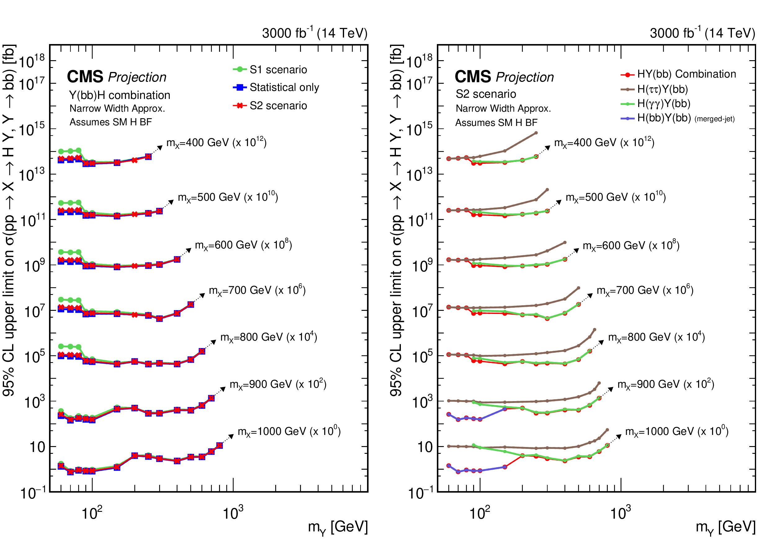
png pdf	Figure 50: Expected upper limits at 95% CL, on the product of the cross section $ \sigma $ for the production of a resonance X via gluon-gluon fusion and the branching fraction $ \mathcal{B} $ for the $ \mathrm{X}\to{\mathrm{Y}}(\mathrm{b}\mathrm{b})\mathrm{H} $ decay, as functions of $ m_{{\mathrm{Y}}} $, for $ m_{\mathrm{X}}\leq $ 1 TeV. For the branching fractions of the $ \mathrm{H}\to\tau\tau $, $ \mathrm{H}\to\gamma\gamma $ and $ \mathrm{H}\to\mathrm{b}\mathrm{b} $ decays, the SM values are assumed. The limits are obtained from the combined likelihood analysis of all analyses discussed in Section 3.3 and shown in Fig. 29, projected to an integrated luminosity of 3000 fb$ ^{-1} $. Shown are the projections for the combined likelihood analysis for different systematic uncertainty scenarios (left), and the projections for the combined likelihood analysis and the individual contributing analyses assuming the S2 scenario (right). For presentation purposes, the limits have been scaled in successive steps by two orders of magnitude. For each set of graphs, a black arrow points to the $ m_{\mathrm{X}} $ related legend.
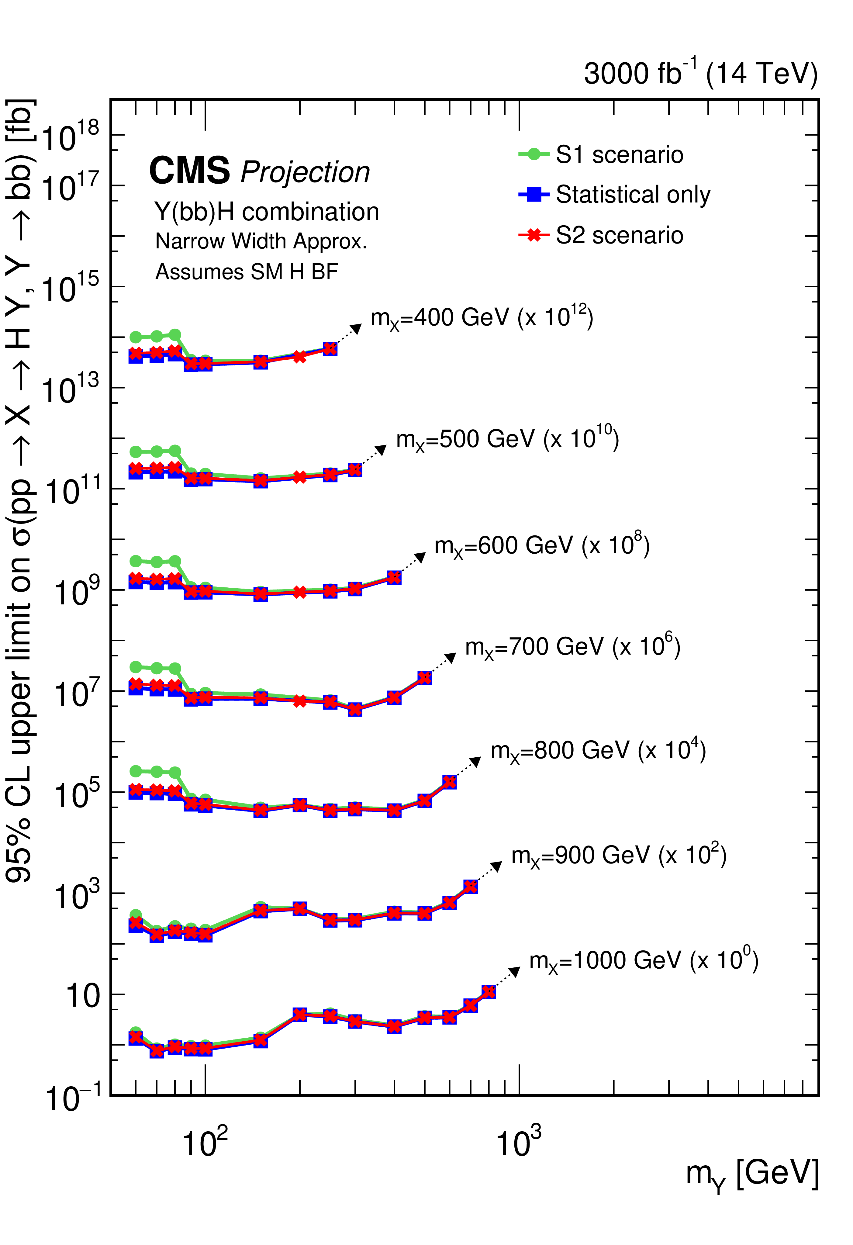
png pdf	Figure 50-a: Expected upper limits at 95% CL, on the product of the cross section $ \sigma $ for the production of a resonance X via gluon-gluon fusion and the branching fraction $ \mathcal{B} $ for the $ \mathrm{X}\to{\mathrm{Y}}(\mathrm{b}\mathrm{b})\mathrm{H} $ decay, as functions of $ m_{{\mathrm{Y}}} $, for $ m_{\mathrm{X}}\leq $ 1 TeV. For the branching fractions of the $ \mathrm{H}\to\tau\tau $, $ \mathrm{H}\to\gamma\gamma $ and $ \mathrm{H}\to\mathrm{b}\mathrm{b} $ decays, the SM values are assumed. The limits are obtained from the combined likelihood analysis of all analyses discussed in Section 3.3 and shown in Fig. 29, projected to an integrated luminosity of 3000 fb$ ^{-1} $. Shown are the projections for the combined likelihood analysis for different systematic uncertainty scenarios (left), and the projections for the combined likelihood analysis and the individual contributing analyses assuming the S2 scenario (right). For presentation purposes, the limits have been scaled in successive steps by two orders of magnitude. For each set of graphs, a black arrow points to the $ m_{\mathrm{X}} $ related legend.
png pdf	Figure 50-b: Expected upper limits at 95% CL, on the product of the cross section $ \sigma $ for the production of a resonance X via gluon-gluon fusion and the branching fraction $ \mathcal{B} $ for the $ \mathrm{X}\to{\mathrm{Y}}(\mathrm{b}\mathrm{b})\mathrm{H} $ decay, as functions of $ m_{{\mathrm{Y}}} $, for $ m_{\mathrm{X}}\leq $ 1 TeV. For the branching fractions of the $ \mathrm{H}\to\tau\tau $, $ \mathrm{H}\to\gamma\gamma $ and $ \mathrm{H}\to\mathrm{b}\mathrm{b} $ decays, the SM values are assumed. The limits are obtained from the combined likelihood analysis of all analyses discussed in Section 3.3 and shown in Fig. 29, projected to an integrated luminosity of 3000 fb$ ^{-1} $. Shown are the projections for the combined likelihood analysis for different systematic uncertainty scenarios (left), and the projections for the combined likelihood analysis and the individual contributing analyses assuming the S2 scenario (right). For presentation purposes, the limits have been scaled in successive steps by two orders of magnitude. For each set of graphs, a black arrow points to the $ m_{\mathrm{X}} $ related legend.
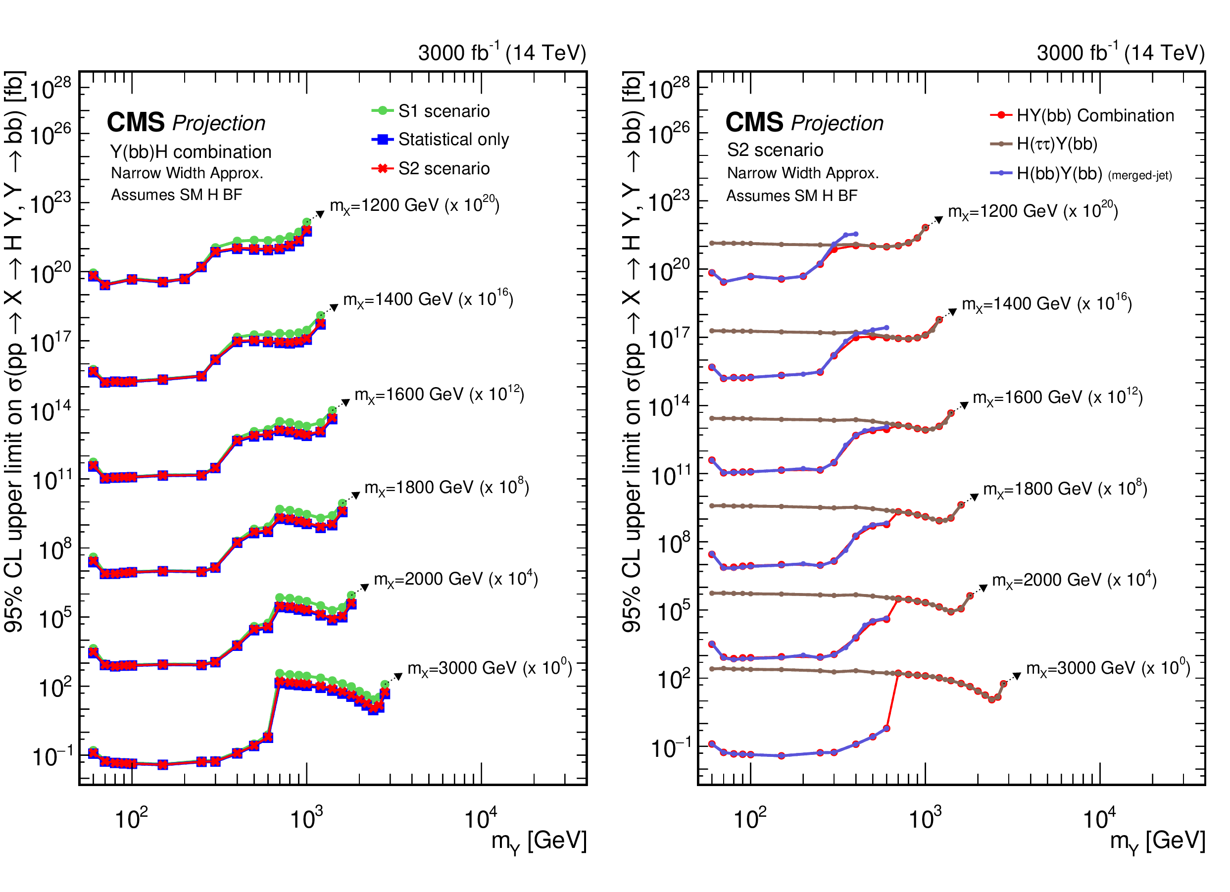
png pdf	Figure 51: Expected upper limits at 95% CL, on the product of the cross section $ \sigma $ for the production of a resonance X via gluon-gluon fusion and the branching fraction $ \mathcal{B} $ for the $ \mathrm{X}\to{\mathrm{Y}}(\mathrm{b}\mathrm{b})\mathrm{H} $ decay, as functions of $ m_{{\mathrm{Y}}} $, for $ m_{\mathrm{X}}\geq $ 1.2 TeV. For the branching fractions of the $ \mathrm{H}\to\tau\tau $ and $ \mathrm{H}\to\mathrm{b}\mathrm{b} $ decays, the SM values are assumed. The limits are obtained from the combined likelihood analysis of all analyses discussed in Section 3.3 and shown in Fig. 30, projected to an integrated luminosity of 3000 fb$ ^{-1} $. Shown are the projections for the combined likelihood analysis for different systematic uncertainty scenarios (left), and the projections for the combined likelihood analysis and the individual contributing analyses assuming the S2 scenario (right). For presentation purposes, the limits have been scaled in successive steps by four orders of magnitude. For each set of graphs, a black arrow points to the $ m_{\mathrm{X}} $ related legend.
png pdf	Figure 51-a: Expected upper limits at 95% CL, on the product of the cross section $ \sigma $ for the production of a resonance X via gluon-gluon fusion and the branching fraction $ \mathcal{B} $ for the $ \mathrm{X}\to{\mathrm{Y}}(\mathrm{b}\mathrm{b})\mathrm{H} $ decay, as functions of $ m_{{\mathrm{Y}}} $, for $ m_{\mathrm{X}}\geq $ 1.2 TeV. For the branching fractions of the $ \mathrm{H}\to\tau\tau $ and $ \mathrm{H}\to\mathrm{b}\mathrm{b} $ decays, the SM values are assumed. The limits are obtained from the combined likelihood analysis of all analyses discussed in Section 3.3 and shown in Fig. 30, projected to an integrated luminosity of 3000 fb$ ^{-1} $. Shown are the projections for the combined likelihood analysis for different systematic uncertainty scenarios (left), and the projections for the combined likelihood analysis and the individual contributing analyses assuming the S2 scenario (right). For presentation purposes, the limits have been scaled in successive steps by four orders of magnitude. For each set of graphs, a black arrow points to the $ m_{\mathrm{X}} $ related legend.
png pdf	Figure 51-b: Expected upper limits at 95% CL, on the product of the cross section $ \sigma $ for the production of a resonance X via gluon-gluon fusion and the branching fraction $ \mathcal{B} $ for the $ \mathrm{X}\to{\mathrm{Y}}(\mathrm{b}\mathrm{b})\mathrm{H} $ decay, as functions of $ m_{{\mathrm{Y}}} $, for $ m_{\mathrm{X}}\geq $ 1.2 TeV. For the branching fractions of the $ \mathrm{H}\to\tau\tau $ and $ \mathrm{H}\to\mathrm{b}\mathrm{b} $ decays, the SM values are assumed. The limits are obtained from the combined likelihood analysis of all analyses discussed in Section 3.3 and shown in Fig. 30, projected to an integrated luminosity of 3000 fb$ ^{-1} $. Shown are the projections for the combined likelihood analysis for different systematic uncertainty scenarios (left), and the projections for the combined likelihood analysis and the individual contributing analyses assuming the S2 scenario (right). For presentation purposes, the limits have been scaled in successive steps by four orders of magnitude. For each set of graphs, a black arrow points to the $ m_{\mathrm{X}} $ related legend.
png pdf	Figure 52: Expected upper limits at 95 % CL on the product of the cross section $ \sigma $ for the production of a resonance X via gluon-gluon fusion and the branching fraction $ \mathcal{B} $ for the $ \mathrm{X}\to{\mathrm{Y}}(\mathrm{b}\mathrm{b})\mathrm{H} $ decay, as obtained from the combined likelihood analysis of the individual analyses presented in Section 3.3 and Figure 29. The results are shown in the plane spanned by $ m_{{\mathrm{Y}}} $ and $ m_{\mathrm{X}} $ for $ m_{\mathrm{X}}\le $ 1 TeV, and projected to an integrated luminosity of 3000 fb$ ^{-1} $, assuming the S2 systematic uncertainty scenario. The numbers in the boxes are given in fb.
png pdf	Figure 53: Interpretation of the upper limits at 95% CL, on the product of the cross section $ \sigma $ for the production of a resonance X via gluon-gluon fusion and the branching fraction $ \mathcal{B} $ for the $ \mathrm{X}\to{\mathrm{Y}}(\mathrm{b}\mathrm{b})\mathrm{H} $ decay, obtained from the projections to an integrated luminosity of 3000 fb$ ^{-1} $ of the (upper left) $ {\mathrm{Y}}(\mathrm{b}\mathrm{b})\mathrm{H}(\gamma\gamma) $ [116], (upper right) $ {\mathrm{Y}}(\mathrm{b}\mathrm{b})\mathrm{H}(\tau\tau) $ [115], and (lower row) $ {\mathrm{Y}}(\mathrm{b}\mathrm{b})\mathrm{H}(\mathrm{b}\mathrm{b}) $ [117] analyses, assuming the S2 systematic uncertainty scenario. The projected limits are mapped onto the ($ m_{\mathrm{X}} $, $ m_{{\mathrm{Y}}} $) plane, and compared with the maximally allowed cross sections of the NMSSM (left and upper right), and TRSM models (lower right) discussed in Section 4.1.3. The points indicate the available theory predictions. The mass dependences of both the projected experimental limits and the maximally allowed theory cross sections have been interpolated to obtain approximate exclusion contours. The NMSSM predictions based on NMSSMTOOLS version 5.6.2 are adapted from Ref. [193], whereas the TRSM is described in Ref. [12]. In both cases, the model predictions have been scaled to $ \sqrt{s}= $ 14 TeV.
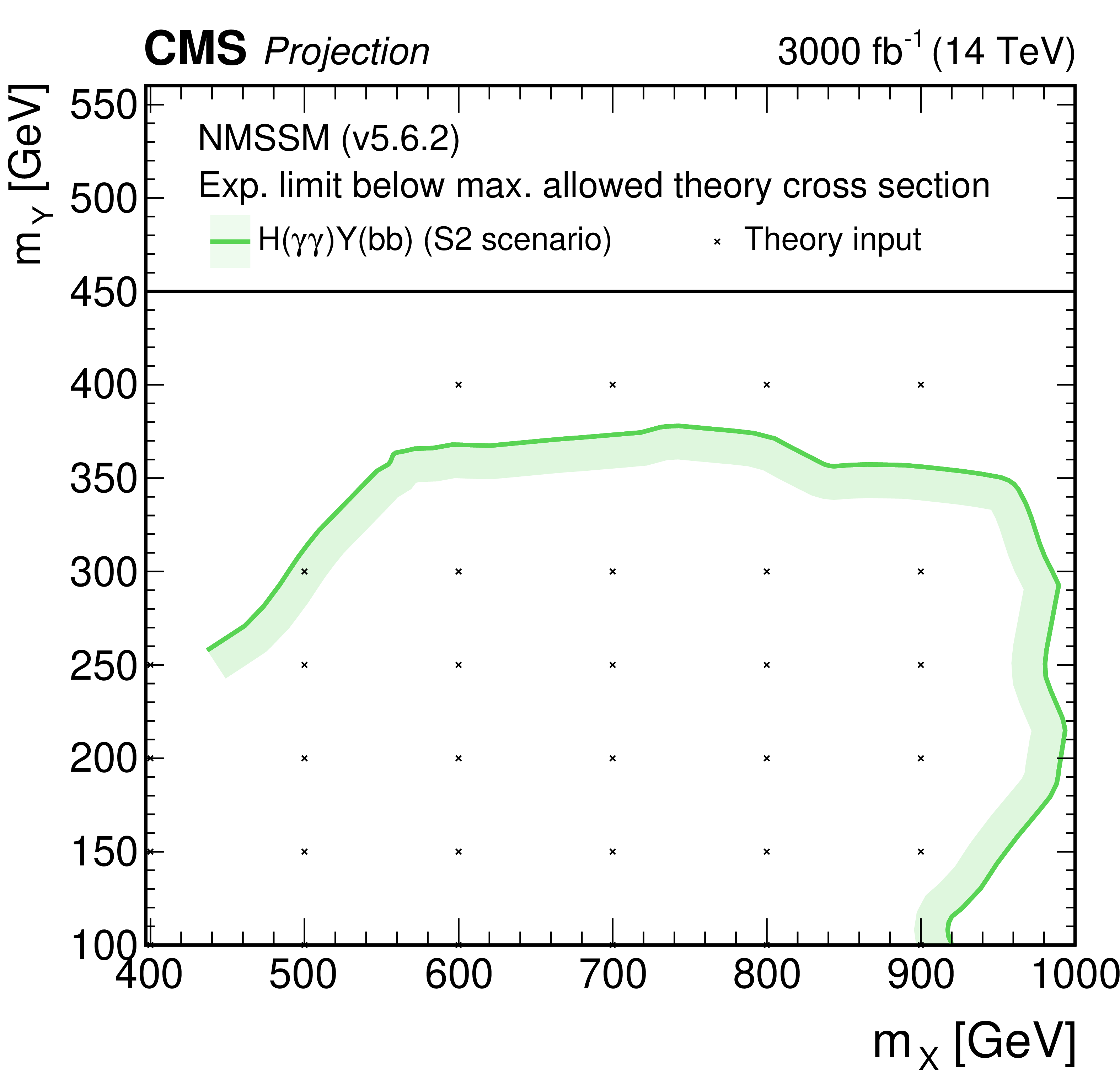
png pdf	Figure 53-a: Interpretation of the upper limits at 95% CL, on the product of the cross section $ \sigma $ for the production of a resonance X via gluon-gluon fusion and the branching fraction $ \mathcal{B} $ for the $ \mathrm{X}\to{\mathrm{Y}}(\mathrm{b}\mathrm{b})\mathrm{H} $ decay, obtained from the projections to an integrated luminosity of 3000 fb$ ^{-1} $ of the (upper left) $ {\mathrm{Y}}(\mathrm{b}\mathrm{b})\mathrm{H}(\gamma\gamma) $ [116], (upper right) $ {\mathrm{Y}}(\mathrm{b}\mathrm{b})\mathrm{H}(\tau\tau) $ [115], and (lower row) $ {\mathrm{Y}}(\mathrm{b}\mathrm{b})\mathrm{H}(\mathrm{b}\mathrm{b}) $ [117] analyses, assuming the S2 systematic uncertainty scenario. The projected limits are mapped onto the ($ m_{\mathrm{X}} $, $ m_{{\mathrm{Y}}} $) plane, and compared with the maximally allowed cross sections of the NMSSM (left and upper right), and TRSM models (lower right) discussed in Section 4.1.3. The points indicate the available theory predictions. The mass dependences of both the projected experimental limits and the maximally allowed theory cross sections have been interpolated to obtain approximate exclusion contours. The NMSSM predictions based on NMSSMTOOLS version 5.6.2 are adapted from Ref. [193], whereas the TRSM is described in Ref. [12]. In both cases, the model predictions have been scaled to $ \sqrt{s}= $ 14 TeV.
png pdf	Figure 53-b: Interpretation of the upper limits at 95% CL, on the product of the cross section $ \sigma $ for the production of a resonance X via gluon-gluon fusion and the branching fraction $ \mathcal{B} $ for the $ \mathrm{X}\to{\mathrm{Y}}(\mathrm{b}\mathrm{b})\mathrm{H} $ decay, obtained from the projections to an integrated luminosity of 3000 fb$ ^{-1} $ of the (upper left) $ {\mathrm{Y}}(\mathrm{b}\mathrm{b})\mathrm{H}(\gamma\gamma) $ [116], (upper right) $ {\mathrm{Y}}(\mathrm{b}\mathrm{b})\mathrm{H}(\tau\tau) $ [115], and (lower row) $ {\mathrm{Y}}(\mathrm{b}\mathrm{b})\mathrm{H}(\mathrm{b}\mathrm{b}) $ [117] analyses, assuming the S2 systematic uncertainty scenario. The projected limits are mapped onto the ($ m_{\mathrm{X}} $, $ m_{{\mathrm{Y}}} $) plane, and compared with the maximally allowed cross sections of the NMSSM (left and upper right), and TRSM models (lower right) discussed in Section 4.1.3. The points indicate the available theory predictions. The mass dependences of both the projected experimental limits and the maximally allowed theory cross sections have been interpolated to obtain approximate exclusion contours. The NMSSM predictions based on NMSSMTOOLS version 5.6.2 are adapted from Ref. [193], whereas the TRSM is described in Ref. [12]. In both cases, the model predictions have been scaled to $ \sqrt{s}= $ 14 TeV.
png pdf	Figure 53-c: Interpretation of the upper limits at 95% CL, on the product of the cross section $ \sigma $ for the production of a resonance X via gluon-gluon fusion and the branching fraction $ \mathcal{B} $ for the $ \mathrm{X}\to{\mathrm{Y}}(\mathrm{b}\mathrm{b})\mathrm{H} $ decay, obtained from the projections to an integrated luminosity of 3000 fb$ ^{-1} $ of the (upper left) $ {\mathrm{Y}}(\mathrm{b}\mathrm{b})\mathrm{H}(\gamma\gamma) $ [116], (upper right) $ {\mathrm{Y}}(\mathrm{b}\mathrm{b})\mathrm{H}(\tau\tau) $ [115], and (lower row) $ {\mathrm{Y}}(\mathrm{b}\mathrm{b})\mathrm{H}(\mathrm{b}\mathrm{b}) $ [117] analyses, assuming the S2 systematic uncertainty scenario. The projected limits are mapped onto the ($ m_{\mathrm{X}} $, $ m_{{\mathrm{Y}}} $) plane, and compared with the maximally allowed cross sections of the NMSSM (left and upper right), and TRSM models (lower right) discussed in Section 4.1.3. The points indicate the available theory predictions. The mass dependences of both the projected experimental limits and the maximally allowed theory cross sections have been interpolated to obtain approximate exclusion contours. The NMSSM predictions based on NMSSMTOOLS version 5.6.2 are adapted from Ref. [193], whereas the TRSM is described in Ref. [12]. In both cases, the model predictions have been scaled to $ \sqrt{s}= $ 14 TeV.
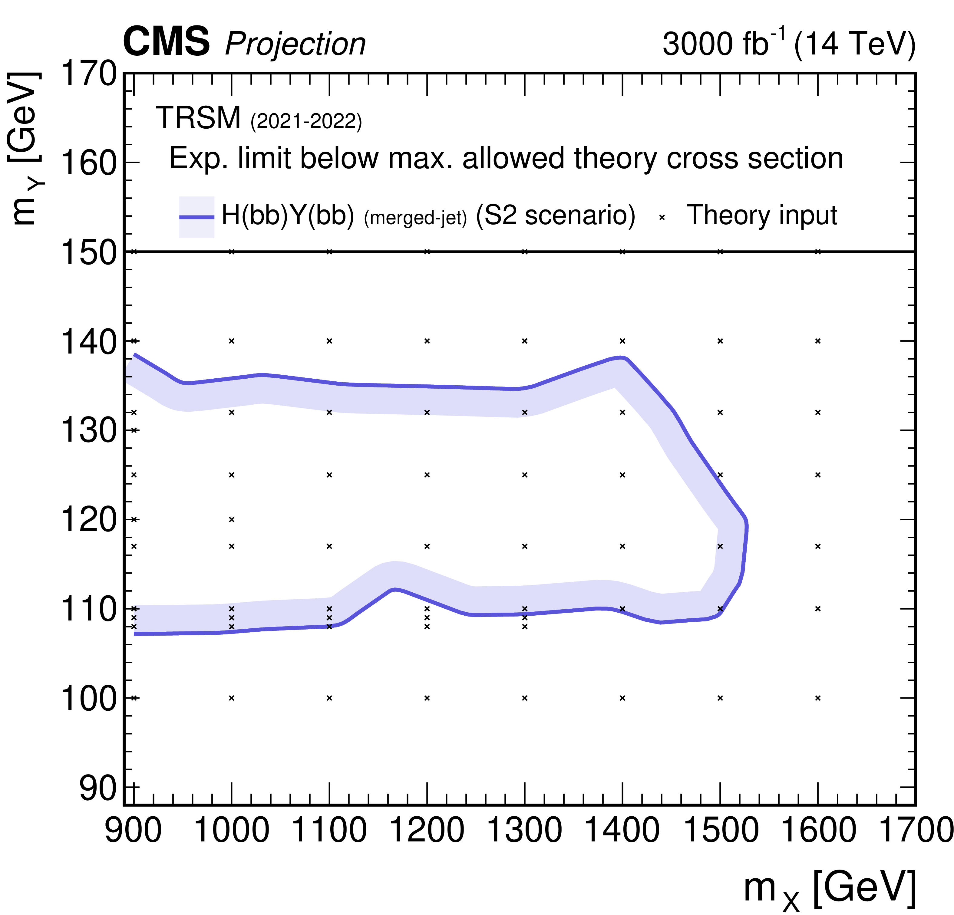
png pdf	Figure 53-d: Interpretation of the upper limits at 95% CL, on the product of the cross section $ \sigma $ for the production of a resonance X via gluon-gluon fusion and the branching fraction $ \mathcal{B} $ for the $ \mathrm{X}\to{\mathrm{Y}}(\mathrm{b}\mathrm{b})\mathrm{H} $ decay, obtained from the projections to an integrated luminosity of 3000 fb$ ^{-1} $ of the (upper left) $ {\mathrm{Y}}(\mathrm{b}\mathrm{b})\mathrm{H}(\gamma\gamma) $ [116], (upper right) $ {\mathrm{Y}}(\mathrm{b}\mathrm{b})\mathrm{H}(\tau\tau) $ [115], and (lower row) $ {\mathrm{Y}}(\mathrm{b}\mathrm{b})\mathrm{H}(\mathrm{b}\mathrm{b}) $ [117] analyses, assuming the S2 systematic uncertainty scenario. The projected limits are mapped onto the ($ m_{\mathrm{X}} $, $ m_{{\mathrm{Y}}} $) plane, and compared with the maximally allowed cross sections of the NMSSM (left and upper right), and TRSM models (lower right) discussed in Section 4.1.3. The points indicate the available theory predictions. The mass dependences of both the projected experimental limits and the maximally allowed theory cross sections have been interpolated to obtain approximate exclusion contours. The NMSSM predictions based on NMSSMTOOLS version 5.6.2 are adapted from Ref. [193], whereas the TRSM is described in Ref. [12]. In both cases, the model predictions have been scaled to $ \sqrt{s}= $ 14 TeV.

Tables
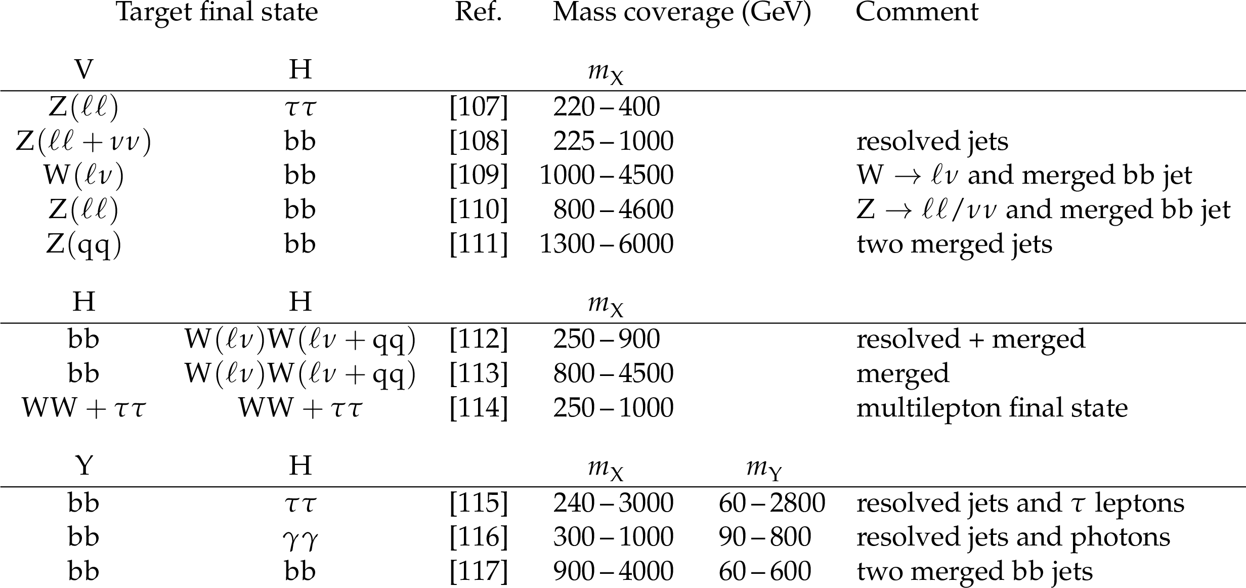
png pdf	Table 1: Summary of all analyses discussed in Section 2. Note that the list of sub-channels is not exhaustive in all cases. All analyses listed under YH also contribute to the HH measurements.
png pdf	Table 2: Searches for resonant HH and YH production considered for the projection study.

Summary

The analyses searching for the production of the Higgs (H) boson through decays of heavy resonances, performed by the CMS Collaboration using the Run 2 data set, are reviewed. This review covers final states with two bosons with at least one an H boson, namely an H boson and a vector boson (VH), a pair of H bosons (HH), and an H boson joined by a new boson Y (YH), where V represents a W or a Z boson. The analyses cover a wide range of H boson decay modes, in particular, decays into photons, b quarks, $ \tau $ leptons, and W bosons. The Y boson is exclusively searched for in b quark final states. Topologies involving both resolved and merged jet objects are used to cover a wide range of the phase space. Multivariate methods are employed in various ways to improve the performance. The results are presented as summary plots which show the sensitivity of all channels in direct comparison. For the HH and YH final states, the results obtained by combining all decay channels are presented for the first time. The results are interpreted in the context of relevant beyond-the-standard model scenarios for resonances decaying into VH, HH and YH final states. These include various extended Higgs sector models, warped extra-dimension models, and heavy vector triplet models. The results from resonant H boson production searches are compared with results from searches in other channels. While all presented analyses assume the validity of the narrow-width approximation, a dedicated study of the impact of finite width and interference is performed for the first time in CMS for the real singlet extension of the standard model. This study shows the modification of the HH cross section and line shape in regions of the parameter space where the narrow-width approximation is not valid anymore. The expected sensitivity of the analyses in the HH and YH final states is estimated for future data sets with integrated luminosities of 300, 1000, and 3000 fb$ ^{-1} $, the last number corresponding to the baseline scenario of the High-Luminosity LHC (HL-LHC) over its full lifetime. The expected upper limits for resonant HH production for the HL-LHC scenario range from about 50 fb at a resonance mass of 300 GeV to nearly 0.01 fb for masses of 3 TeV and above. The exclusions in terms of $ \tan\beta $ in the hMSSM and $ M^{125}_{\text{h,EFT}} $ scenarios are expanded by almost a factor of two compared to the Run 2 data set. This review shows how the specific strengths of many different experimental signatures can be combined to chart very thoroughly the territory where resonant Higgs boson production might reveal beyond the standard model physics, and gives a promising outlook towards the achievement potential of future measurements in this sector.

Additional Figures
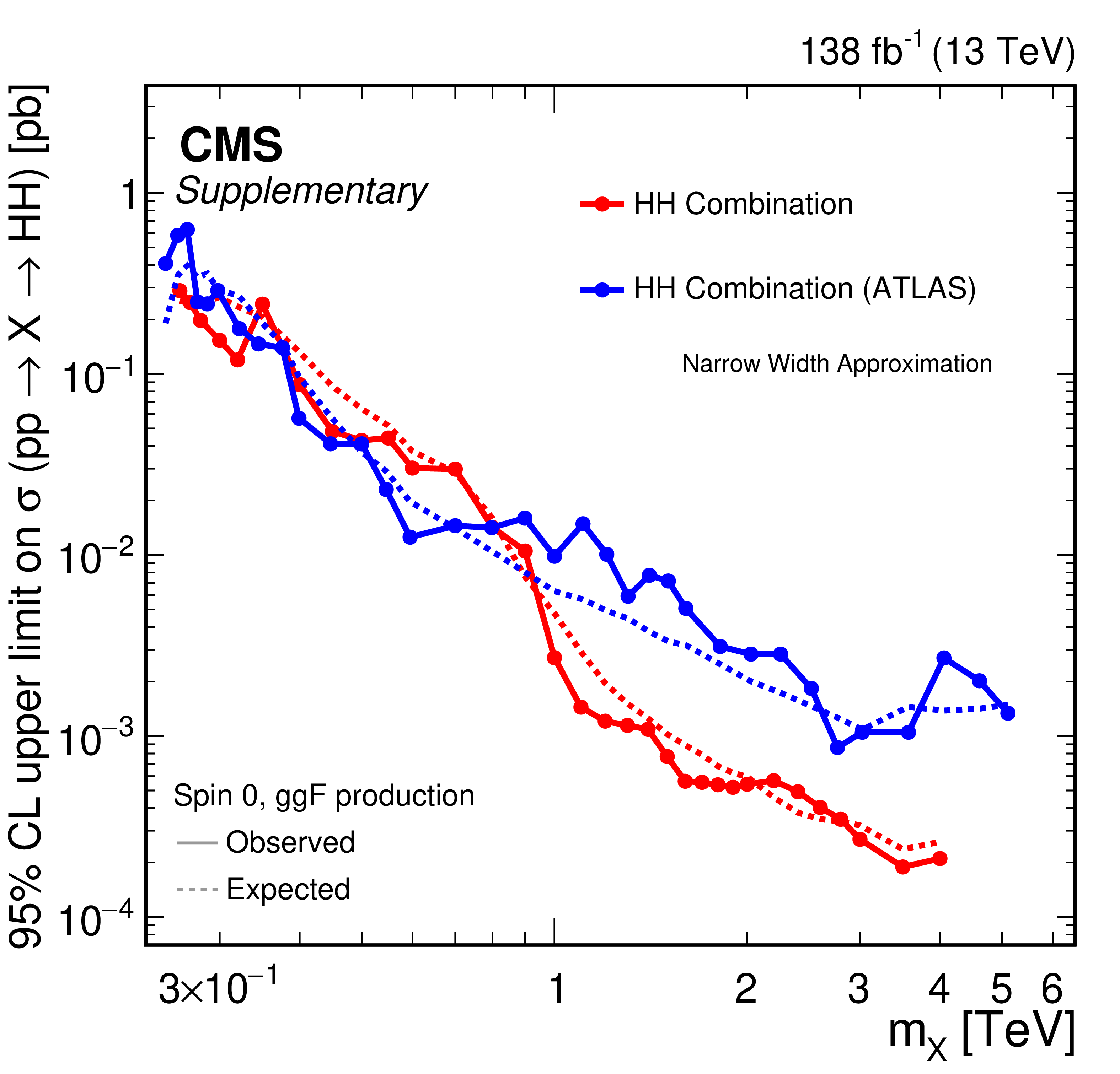
png pdf	Additional Figure 1: Observed and expected 95% CL upper limits on the product of the cross section $ \sigma $ for the production of a spin-0 resonance X, via gluon-gluon fusion and the branching fraction $ \mathcal{B} $ for the decay into a pair of H bosons. The combined results of the CMS analyses are shown in red, while the combination from ATLAS [168] is shown in blue. The observed limits are indicated by markers connected with solid lines and the expected limits by dashed lines.
png pdf	Additional Figure 2: Observed and expected upper limits at 95% CL, on the product of the cross section $ \sigma $ for the production of a resonance X via gluon-gluon fusion and the branching fraction $ \mathcal{B} $ for the $ \mathrm{X}\to{\mathrm{Y}}(\mathrm{b}\mathrm{b})\mathrm{H} $ decay, as obtained from a combined likelihood analysis of several individual channels. The results are presented as a function of $ m_{\mathrm{X}} $ for six values of $ m_{{\mathrm{Y}}} $. The corresponding maximally allowed values of $ \sigma\mathcal{B} $ in the NMSSM are also shown for comparison, as adapted from Ref. [193], which accounts for experimental constraints as defined in version 5.6.2 of the program NMSSMTOOLS.

References
1	ATLAS Collaboration	Observation of a new particle in the search for the standard model Higgs boson with the ATLAS detector at the LHC	PLB 716 (2012) 1	1207.7214
2	CMS Collaboration	Observation of a new boson at a mass of 125 GeV with the CMS experiment at the LHC	PLB 716 (2012) 30	CMS-HIG-12-028 1207.7235
3	CMS Collaboration	Observation of a new boson with mass near 125 GeV in pp collisions at $ \sqrt{s} = $ 7 and 8 TeV	JHEP 06 (2013) 081	CMS-HIG-12-036 1303.4571
4	CMS Collaboration	A portrait of the Higgs boson by the CMS experiment ten years after the discovery	Nature 607 (2022) 60	CMS-HIG-22-001 2207.00043
5	T. D. Lee	A theory of spontaneous $ T $ violation	PRD 8 (1973) 1226
6	G. C. Branco et al.	Theory and phenomenology of two-Higgs-doublet models	Phys. Rept. 516 (2012) 1	1106.0034
7	H. E. Haber and O. St \aa l	New LHC benchmarks for the $ \mathcal{CP} $-conserving two-Higgs-doublet model	EPJC 75 (2015) 491	1507.04281
8	F. Kling, J. M. No, and S. Su	Anatomy of exotic Higgs decays in 2HDM	JHEP 09 (2016) 093	1604.01406
9	G. Chalons and F. Domingo	Analysis of the Higgs potentials for two doublets and a singlet	PRD 86 (2012) 115024	1209.6235
10	C.-Y. Chen, M. Freid, and M. Sher	Next-to-minimal two Higgs doublet model	PRD 89 (2014) 075009	1312.3949
11	M. Mühlleitner, M. O. P. Sampaio, R. Santos, and J. Wittbrodt	The N2HDM under theoretical and experimental scrutiny	JHEP 03 (2017) 094	1612.01309
12	T. Robens, T. Stefaniak, and J. Wittbrodt	Two-real-scalar-singlet extension of the SM: LHC phenomenology and benchmark scenarios	EPJC 80 (2020) 151	1908.08554
13	J. F. Gunion and H. E. Haber	Higgs bosons in supersymmetric models (1)	NPB 272 (1986) 1
14	J. F. Gunion and H. E. Haber	Higgs bosons in supersymmetric models (II). Implications for phenomenology	NPB 278 (1986) 449
15	G. Degrassi et al.	Towards high precision predictions for the MSSM Higgs sector	EPJC 28 (2003) 133	hep-ph/0212020
16	A. Djouadi	The anatomy of electroweak symmetry breaking Tome II: The Higgs bosons in the minimal supersymmetric model	Phys. Rept. 459 (2008) 1	hep-ph/0503173
17	M. Maniatis	The next-to-minimal supersymmetric extension of the standard model reviewed	Int. J. Mod. Phys. A 25 (2010) 3505	0906.0777
18	U. Ellwanger, C. Hugonie, and A. M. Teixeira	The next-to-minimal supersymmetric standard model	Phys. Rept. 496 (2010) 1	0910.1785
19	S. F. King, M. Mühlleitner, and R. Nevzorov	NMSSM Higgs benchmarks near 125 GeV	Nucl. Phys. B. 860 (2012) 207	1201.2671
20	L. Randall and R. Sundrum	Large mass hierarchy from a small extra dimension	PRL 83 (1999) 3370	hep-ph/9905221
21	W. D. Goldberger and M. B. Wise	Modulus stabilization with bulk fields	PRL 83 (1999) 4922	hep-ph/9907447
22	O. DeWolfe, D. Z. Freedman, S. S. Gubser, and A. Karch	Modeling the fifth dimension with scalars and gravity	PRD 62 (2000) 046008	hep-th/9909134
23	C. Csàki, M. Graesser, L. Randall, and J. Terning	Cosmology of brane models with radion stabilization	PRD 62 (2000) 045015	hep-ph/9911406
24	H. Davoudiasl, J. L. Hewett, and T. G. Rizzo	Phenomenology of the Randall--Sundrum gauge hierarchy model	PRL 84 (2000) 2080	hep-ph/9909255
25	C. Csaki, M. L. Graesser, and G. D. Kribs	Radion dynamics and electroweak physics	PRD 63 (2001) 065002	hep-th/0008151
26	K. Agashe, H. Davoudiasl, G. Perez, and A. Soni	Warped gravitons at the CERN LHC and beyond	PRD 76 (2007) 036006	hep-ph/0701186
27	A. L. Fitzpatrick, J. Kaplan, L. Randall, and L.-T. Wang	Searching for the Kaluza-Klein graviton in bulk RS models	JHEP 09 (2007) 013	hep-ph/0701150
28	A. Oliveira	Gravity particles from warped extra dimensions, predictions for LHC		1404.0102
29	G. F. Giudice, R. Rattazzi, and J. D. Wells	Graviscalars from higher-dimensional metrics and curvature-Higgs mixing	NPB 595 (2001) 250	hep-ph/0002178
30	D. Pappadopulo, A. Thamm, R. Torre, and A. Wulzer	Heavy vector triplets: Bridging theory and data	JHEP 09 (2014) 060	1402.4431
31	CMS Collaboration	HEPData record for this analysis	link
32	P. W. Higgs	Broken symmetries, massless particles and gauge fields	PL 12 (1964) 132
33	P. W. Higgs	Spontaneous symmetry breakdown without massless bosons	PR 145 (1966) 1156
34	F. Englert and R. Brout	Broken symmetry and the mass of gauge vector mesons	PRL 13 (1964) 321
35	M. Cepeda et al.	Handbook of LHC Higgs cross sections: 4. Deciphering the nature of the Higgs sector	CERN Report CERN-2017-002-M, 2016 link	1610.07922
36	ATLAS Collaboration	Measurement of the Higgs boson mass with $ \mathrm{H}\to\gamma\gamma $ decays in 140 fb$ ^{-1} $ of $ \sqrt{s}= $13\,TeV pp collisions with the ATLAS detector	PLB 847 (2023) 138315	2308.07216
37	CMS Collaboration	Measurement of the Higgs boson width and evidence of its off-shell contributions to ZZ production	Nature Phys. 18 (2022) 1329	CMS-HIG-21-013 2202.06923
38	LHC Higgs Cross Section Working Group	Handbook of LHC Higgs Cross Sections: 3. Higgs Properties: Report of the LHC Higgs Cross Section Working Group	in CERN Yellow Reports: Monographs, 2013 CERN-2013-004
39	F. Bezrukov and M. Shaposhnikov	Inflation, LHC and the Higgs boson	C. R. Phys. 16 (2015) 994
40	F. L. Bezrukov and M. Shaposhnikov	The standard model Higgs boson as the inflaton	PLB 659 (2008) 703	0710.3755
41	Y. Hamada and M. Yamada	Baryogenesis in false vacuum	EPJC 77 (2017) 643	1605.06897
42	I. P. Ivanov	Building and testing models with extended Higgs sectors	Prog. Part. Nucl. Phys. 95 (2017) 160	1702.03776
43	S. Dawson, C. Englert, and T. Plehn	Higgs Physics: It ain't over till it's over	Phys. Rept. 816 (2019) 1	1808.01324
44	J. Steggemann	Extended scalar sectors	Ann. Rev. Nucl. Part. Sci. 70 (2020) 197
45	Particle Data Group	Review of particle physics	Prog. Theor. Exp. Phys. 2022 (2022) 083C01
46	C. Englert et al.	Precision measurements of Higgs couplings: Implications for new physics scales	JPG 41 (2014) 113001	1403.7191
47	CMS Collaboration	Combined measurements of Higgs boson couplings in proton-proton collisions at $ \sqrt{s}=$ 13 TeV	EPJC 79 (2019) 421	CMS-HIG-17-031 1809.10733
48	ATLAS Collaboration	Combined measurements of Higgs boson production and decay using up to 80 fb$ ^{-1} $ of proton-proton collision data at $ \sqrt{s}= $ 13 TeV collected with the ATLAS experiment	PRD 101 (2020) 012002	1909.02845
49	ATLAS Collaboration	A detailed map of Higgs boson interactions by the ATLAS experiment ten years after the discovery	Nature 607 (2022) 52	2207.00092
50	A. Datta and A. Raychaudhuri	Next-to-minimal Higgs: Mass bounds and search prospects	PRD 57 (1998) 2940	hep-ph/9708444
51	V. Barger et al.	Complex singlet extension of the standard model	PRD 79 (2009) 015018	0811.0393
52	R. Costa, M. Mühlleitner, M. O. P. Sampaio, and R. Santos	Singlet extensions of the standard model at LHC Run 2: Benchmarks and comparison with the NMSSM	JHEP 06 (2016) 034	1512.05355
53	T. Robens and T. Stefaniak	Status of the Higgs singlet extension of the standard model after LHC Run 1	EPJC 75 (2015) 104	1501.02234
54	J. Haller et al.	Update of the global electroweak fit and constraints on two-Higgs-doublet models	EPJC 78 (2018) 675	1803.01853
55	D. Eriksson, J. Rathsman, and O. Stal	2HDMC: Two-Higgs-doublet model calculator physics and manual	Comput. Phys. Commun. 181 (2010) 189	0902.0851
56	R. Harlander et al.	Interim recommendations for the evaluation of Higgs production cross sections and branching ratios at the LHC in the two-Higgs-doublet model		1312.5571
57	A. Djouadi and J. Quevillon	The MSSM Higgs sector at a high $ M_{\text{SUSY}} $: Reopening the low $ \tan\beta $ regime and heavy Higgs searches	JHEP 10 (2013) 028	1304.1787
58	A. Djouadi et al.	The post-Higgs MSSM scenario: Habemus MSSM?	EPJC 73 (2013) 2650	1307.5205
59	A. Djouadi et al.	Fully covering the MSSM Higgs sector at the LHC	JHEP 06 (2015) 168	1502.05653
60	H. Bahl, S. Liebler, and T. Stefaniak	MSSM Higgs benchmark scenarios for Run 2 and beyond: The low $ \tan\beta $ region	EPJC 79 (2019) 279	1901.05933
61	E. A. Bagnaschi et al.	Benchmark scenarios for MSSM Higgs boson searches at the LHC	Technical Report LHCHWG-2021-001, 2021 link
62	LHC Higgs Working Group -- MSSM subgroup	LHCHWG MSSM ROOT files
63	E. Bagnaschi et al.	MSSM Higgs boson searches at the LHC: Benchmark scenarios for Run 2 and beyond	EPJC 79 (2019) 617	1808.07542
64	CMS Collaboration	Searches for additional Higgs bosons and for vector leptoquarks in $ \tau\tau $ final states in proton-proton collisions at $ \sqrt{s} = $ 13 TeV	JHEP 07 (2023) 073	CMS-HIG-21-001 2208.02717
65	I. Engeln, M. Mühlleitner, and J. Wittbrodt	N2HDECAY: Higgs boson decays in the different phases of the N2HDM	Comput. Phys. Commun. 234 (2019) 256	1805.00966
66	H. Abouabid et al.	Benchmarking di-Higgs production in various extended Higgs sector models	JHEP 09 (2022) 011	2112.12515
67	S. Baum and N. R. Shah	Two Higgs doublets and a complex singlet: Disentangling the decay topologies and associated phenomenology	JHEP 12 (2018) 044	1808.02667
68	U. Ellwanger and M. Rodriguez-Vazquez	Simultaneous search for extra light and heavy Higgs bosons via cascade decays	JHEP 11 (2017) 008	1707.08522
69	S. Baum, N. R. Shah, and K. Freese	The NMSSM is within reach of the LHC: Mass correlations \& decay signatures	JHEP 04 (2019) 011	1901.02332
70	D. Dominici, B. Grzadkowski, J. F. Gunion, and M. Toharia	The scalar sector of the Randall--Sundrum model	NPB 671 (2003) 243	hep-ph/0206192
71	I. Antoniadis and R. Sturani	Higgs graviscalar mixing in type I string theory	NPB 631 (2002) 66	hep-th/0201166
72	N. Desai, U. Maitra, and B. Mukhopadhyaya	An updated analysis of radion-Higgs mixing in the light of LHC data	JHEP 10 (2013) 093	1307.3765
73	A. Oliveira and R. Rosenfeld	Graviscalars from higher-dimensional metrics and curvature-Higgs mixing	PLB 702 (2011) 201	1009.4497
74	CMS Collaboration	Search for high-mass resonances in dilepton final states in proton-proton collisions at $ \sqrt{s}= $ 13 TeV	JHEP 06 (2018) 120	CMS-EXO-16-047 1803.06292
75	C. Grojean, E. Salvioni, and R. Torre	A weakly constrained $ \mathrm{W^{'}} $ at the early LHC	JHEP 07 (2011) 002	1103.2761
76	E. Salvioni, G. Villadoro, and F. Zwirner	Minimal $ \mathrm{Z}^{'} $ models: Present bounds and early LHC reach	JHEP 11 (2009) 068	0909.1320
77	G. Altarelli, B. Mele, and M. Ruiz-Altaba	Searching for new heavy vector bosons in $ \mathrm{p}\overline{\mathrm{p}} $ colliders	Z. Phys. C 45 (1989) 109
78	M. Schmaltz and D. Tucker-Smith	Little Higgs review	Ann. Rev. Nucl. Part. Sci. 55 (2005) 229	hep-ph/0502182
79	N. Arkani-Hamed, A. G. Cohen, E. Katz, and A. E. Nelson	The littlest Higgs	JHEP 07 (2002) 034	hep-ph/0206021
80	B. Bellazzini, C. Csàki, and J. Serra	Composite Higgses	EPJC 74 (2014) 2766	1401.2457
81	R. Contino, D. Marzocca, D. Pappadopulo, and R. Rattazzi	On the effect of resonances in composite Higgs phenomenology	JHEP 10 (2011) 081	1109.1570
82	D. Marzocca, M. Serone, and J. Shu	General composite Higgs models	JHEP 08 (2012) 013	1205.0770
83	D. Greco and D. Liu	Hunting composite vector resonances at the LHC: Naturalness facing data	JHEP 12 (2014) 126	1410.2883
84	K. Lane and L. Pritchett	The light composite Higgs boson in strong extended technicolor	JHEP 06 (2017) 140	1604.07085
85	V. D. Barger, W.-Y. Keung, and E. Ma	A gauge model with light W and Z bosons	PRD 22 (1980) 727
86	CMS Collaboration	Search for heavy resonances decaying into two Higgs bosons or into a Higgs boson and a W or Z boson in proton-proton collisions at 13 TeV	JHEP 01 (2019) 051	1808.01365
87	CMS Collaboration	Search for heavy resonances decaying into a vector boson and a Higgs boson in final states with charged leptons, neutrinos and b quarks at $ \sqrt{s}= $ 13 TeV	JHEP 11 (2018) 172	1807.02826
88	CMS Collaboration	Search for heavy resonances that decay into a vector boson and a Higgs boson in hadronic final states at $ \sqrt{s}= $ 13 TeV	EPJC 77 (2017) 636	1707.01303
89	CMS Collaboration	Search for heavy resonances decaying into a vector boson and a Higgs boson in final states with charged leptons, neutrinos, and b quarks	PLB 768 (2017) 137	1610.08066
90	CMS Collaboration	Search for massive $ {\mathrm{W}\mathrm{H}} $ resonances decaying into the $ {\ell\nu\mathrm{b}\overline{\mathrm{b}}} $ final state at $ \sqrt{s}= $ 8 TeV	EPJC 76 (2016) 237	CMS-EXO-14-010 1601.06431
91	CMS Collaboration	Search for a massive resonance decaying into a Higgs boson and a W or Z boson in hadronic final states in proton-proton collisions at $ \sqrt{s}= $ 8 TeV	JHEP 02 (2016) 145	CMS-EXO-14-009 1506.01443
92	CMS Collaboration	Search for narrow high-mass resonances in proton-proton collisions at $ \sqrt{s}= $ 8 TeV decaying to a Z and a Higgs boson	PLB 748 (2015) 255	CMS-EXO-13-007 1502.04994
93	ATLAS Collaboration	Search for heavy resonances decaying into a Z or W boson and a Higgs boson in final states with leptons and b jets in 139 $ $fb$ ^{-1} $ of pp collisions at $ \sqrt{s}=13 $TeV with the ATLAS detector	JHEP 06 (2023) 016	2207.00230
94	ATLAS Collaboration	Search for resonances decaying into a weak vector boson and a Higgs boson in the fully hadronic final state produced in proton-proton collisions at $ \sqrt{s} = $ 13 TeV with the ATLAS detector	PRD 102 (2020) 112008	2007.05293
95	ATLAS Collaboration	Combination of searches for heavy resonances decaying into bosonic and leptonic final states using 36 fb$ ^{-1} $ of proton-proton collision data at $ \sqrt{s} = $ 13 TeV with the ATLAS detector	PRD 98 (2018) 052008	1808.02380
96	ATLAS Collaboration	Search for heavy resonances decaying to a photon and a hadronically decaying $ \mathrm{Z}/\mathrm{W}/\mathrm{H} $ boson in pp collisions at $ \sqrt{s}= $ 13 TeV with the ATLAS detector	PRD 98 (2018) 032015	1805.01908
97	ATLAS Collaboration	Search for heavy resonances decaying into a W or Z boson and a Higgs boson in final states with leptons and b-jets in 36 fb$ ^{-1} $ of $ \sqrt{s} = $ 13 TeV pp collisions with the ATLAS detector	JHEP 03 (2018) 174	1712.06518
98	ATLAS Collaboration	Search for a new resonance decaying to a W or Z boson and a Higgs boson in the $ {\ell\ell/\ell\nu/\nu\nu}+\mathrm{b}\overline{\mathrm{b}} $ final states with the ATLAS detector	EPJC 75 (2015) 263	1503.08089
99	ATLAS Collaboration	Search for new resonances decaying to a W or Z boson and a Higgs boson in the $ \ell^+ \ell^- b\bar b $, $ \ell \nu b\bar b $, and $ \nu\bar{\nu} b\bar b $ channels with pp collisions at $ \sqrt s = $ 13 TeV with the ATLAS detector	PLB 765 (2017) 32	1607.05621
100	ATLAS Collaboration	Search for high-mass diboson resonances with boson-tagged jets in proton-proton collisions at $ \sqrt{s}= $ 8 TeV with the ATLAS detector	JHEP 12 (2015) 055	1506.00962
101	ATLAS Collaboration	Search for a heavy Higgs boson decaying into a Z boson and another heavy Higgs boson in the $ \ell \ell bb $ and $ \ell \ell WW $ final states in pp collisions at $ \sqrt{s}= $ 13 $ \text {TeV} $ with the ATLAS detector	EPJC 81 (2021) 396	2011.05639
102	ATLAS Collaboration	Search for Higgs boson pair production in the two bottom quarks plus two photons final state in pp collisions at $ \sqrt{s}= $ 13 TeV with the ATLAS detector	PRD 106 (2022) 052001	2112.11876
103	ATLAS Collaboration	Search for resonant and non-resonant Higgs boson pair production in the $ \mathrm{b}\overline{\mathrm{b}}{\tau}^{+}{\tau}^{-} $ decay channel using 13 TeV pp collision data from the ATLAS detector	JHEP 07 (2023) 040	2209.10910
104	ATLAS Collaboration	Search for resonant pair production of Higgs bosons in the $ \mathrm{b}\overline{\mathrm{b}}\mathrm{b}\overline{\mathrm{b}} $ final state using pp collisions at $ \sqrt{s} = $ 13 TeV with the ATLAS detector	PRD 105 (2022) 092002	2202.07288
105	ATLAS Collaboration	Search for a new heavy scalar particle decaying into a Higgs boson and a new scalar singlet in final states with one or two light leptons and a pair of $\tau$-leptons with the ATLAS detector	JHEP 10 (2023) 009	2307.11120
106	ATLAS Collaboration	Anomaly detection search for new resonances decaying into a Higgs boson and a generic new particle $ X $ in hadronic final states using $ \sqrt{s} = $ 13 TeV pp collisions with the ATLAS detector	PRD 108 (2023) 052009	2306.03637
107	CMS Collaboration	Search for a heavy pseudoscalar Higgs boson decaying into a 125 GeV Higgs boson and a Z boson in final states with two tau and two light leptons at $ \sqrt{s}= $ 13 TeV	JHEP 03 (2020) 065	CMS-HIG-18-023 1910.11634
108	CMS Collaboration	Search for a heavy pseudoscalar boson decaying to a Z and a Higgs boson at $ \sqrt{s} = $ 13 TeV	EPJC 79 (2019) 564	CMS-HIG-18-005 1903.00941
109	CMS Collaboration	Search for heavy resonances decaying to $ {\mathrm{W}\mathrm{W}} $, $ {\mathrm{W}\mathrm{Z}} $, or $ {\mathrm{W}\mathrm{H}} $ boson pairs in the lepton plus merged jet final state in proton-proton collisions at $ \sqrt{s} = $ 13 TeV	PRD 105 (2022) 032008	2109.06055
110	CMS Collaboration	Search for a heavy vector resonance decaying to a Z boson and a Higgs boson in proton-proton collisions at $ \sqrt{s} =$ 13 TeV	EPJC 81 (2021) 688	2102.08198
111	CMS Collaboration	Search for new heavy resonances decaying to WW, WZ, ZZ, WH, or ZH boson pairs in the all-jets final state in proton-proton collisions at $ \sqrt{s}= $ 13 TeV	PLB 844 (2023) 137813	2210.00043
112	CMS Collaboration	Search for Higgs boson pair production in the bbWW decay mode in proton-proton collisions at $ \sqrt{s} = $ 13 TeV	Submitted to JHEP, 2024	CMS-HIG-21-005 2403.09430
113	CMS Collaboration	Search for heavy resonances decaying to a pair of Lorentz-boosted higgs bosons in final states with leptons and a bottom quark pair at $ \sqrt{s} = $ 13 TeV	JHEP 05 (2022) 005	2112.03161
114	CMS Collaboration	Search for Higgs boson pairs decaying to $ \mathrm{W}\mathrm{W}\mathrm{W}\mathrm{W} $, $ \mathrm{W}\mathrm{W}\tau\tau $, and $ \tau\tau\tau\tau $ in proton-proton collisions at $ \sqrt{s} = $ 13 TeV	JHEP 07 (2023) 095	CMS-HIG-21-002 2206.10268
115	CMS Collaboration	Search for a heavy Higgs boson decaying into two lighter Higgs bosons in the $ \tau\tau $bb final state at 13 TeV	JHEP 11 (2021) 057	CMS-HIG-20-014 2106.10361
116	CMS Collaboration	Search for a new resonance decaying into two spin-0 bosons in a final state with two photons and two bottom quarks in proton-proton collisions at $ \sqrt{s} = $ 13 TeV	submitted to JHEP	CMS-HIG-21-011 2310.01643
117	CMS Collaboration	Search for a massive scalar resonance decaying to a light scalar and a Higgs boson in the four b quarks final state with boosted topology	PLB 842 (2023) 137392	2204.12413
118	M. Gouzevitch et al.	Scale-invariant resonance tagging in multijet events and new physics in Higgs pair production	JHEP 07 (2013) 148	1303.6636
119	A. J. Larkoski, I. Moult, and B. Nachman	Jet substructure at the Large Hadron Collider: A review of recent advances in theory and machine learning	Phys. Rept. 841 (2020) 1	1709.04464
120	R. Kogler, B. Nachman, A. Schmidt (editors) et al.	Jet substructure at the Large Hadron Collider	Rev. Mod. Phys. 91 (2019) 045003	1803.06991
121	R. Kogler	Advances in jet substructure at the LHC: Algorithms, measurements and searches for new physical phenomena	volume 284 of Springer Tracts Mod. Phys. Springer, ISBN~978-3-030-72857-1, 978-3-030-72858-8, 2021 link
122	CMS Collaboration	The CMS experiment at the CERN LHC	JINST 3 (2008) S08004
123	CMS Collaboration	Performance of the CMS Level-1 trigger in proton-proton collisions at $ \sqrt{s} = $ 13 TeV	JINST 15 (2020) P10017	CMS-TRG-17-001 2006.10165
124	CMS Collaboration	The CMS trigger system	JINST 12 (2017) P01020	CMS-TRG-12-001 1609.02366
125	CMS Collaboration	Particle-flow reconstruction and global event description with the CMS detector	JINST 12 (2017) P10003	CMS-PRF-14-001 1706.04965
126	CMS Collaboration	Technical proposal for the Phase-II upgrade of the Compact Muon Solenoid	CMS Technical Proposal CMS-TDR-15-02, 2015 CDS
127	M. Cacciari, G. P. Salam, and G. Soyez	The anti-$ k_{\mathrm{T}} $ jet clustering algorithm	JHEP 04 (2008) 063	0802.1189
128	M. Cacciari, G. P. Salam, and G. Soyez	FastJet user manual	EPJC 72 (2012) 1896	1111.6097
129	CMS Collaboration	Jet energy scale and resolution in the CMS experiment in pp collisions at 8 TeV	JINST 12 (2017) P02014	CMS-JME-13-004 1607.03663
130	D. Bertolini, P. Harris, M. Low, and N. Tran	Pileup per particle identification	JHEP 10 (2014) 59	1407.6013
131	CMS Collaboration	Pileup mitigation at CMS in 13 TeV data	JINST 15 (2020) P09018	CMS-JME-18-001 2003.00503
132	CMS Collaboration	Performance of missing transverse momentum reconstruction in proton-proton collisions at $ \sqrt{s} = $ 13 TeV using the CMS detector	JINST 14 (2019) P07004	CMS-JME-17-001 1903.06078
133	CMS Collaboration	Jet algorithms performance in 13 TeV data	CMS Physics Analysis Summary, 2017 CMS-PAS-JME-16-003	CMS-PAS-JME-16-003
134	A. J. Larkoski, S. Marzani, G. Soyez, and J. Thaler	Soft drop	JHEP 05 (2014) 146	1402.2657
135	M. Dasgupta, A. Fregoso, S. Marzani, and G. P. Salam	Towards an understanding of jet substructure	JHEP 09 (2013) 029	1307.0007
136	J. M. Butterworth, A. R. Davison, M. Rubin, and G. P. Salam	Jet substructure as a new Higgs search channel at the LHC	PRL 100 (2008) 242001	0802.2470
137	CMS Collaboration	Identification of heavy-flavour jets with the CMS detector in pp collisions at 13 TeV	JINST 13 (2018) P05011	CMS-BTV-16-002 1712.07158
138	E. Bols et al.	Jet flavour classification using DeepJet	JINST 15 (2020) P12012	2008.10519
139	Y. L. Dokshitzer, G. D. Leder, S. Moretti, and B. R. Webber	Better jet clustering algorithms	JHEP 08 (1997) 001	hep-ph/9707323
140	M. Wobisch and T. Wengler	Hadronization corrections to jet cross-sections in deep inelastic scattering	in Workshop on Monte Carlo Generators for HERA Physics, 1998	hep-ph/9907280
141	CMS Collaboration	Identification of heavy, energetic, hadronically decaying particles using machine-learning techniques	JINST 15 (2020) P06005	CMS-JME-18-002 2004.08262
142	H. Qu and L. Gouskos	ParticleNet: Jet tagging via particle clouds	PRD 101 (2020) 056019	1902.08570
143	CMS Collaboration	Performance of the DeepJet b tagging algorithm using 41.9 fb$ ^{-1} $ of data from proton-proton collisions at 13 TeV with Phase 1 CMS detector	Detector performance note CMS-DP-2018-058, 2018 CDS
144	J. Thaler and K. Van Tilburg	Identifying boosted objects with N-subjettiness	JHEP 03 (2011) 015	1011.2268
145	J. Dolen et al.	Thinking outside the ROCs: Designing decorrelated taggers (DDT) for jet substructure	JHEP 05 (2016) 156	1603.00027
146	CMS Collaboration	Performance of electron reconstruction and selection with the CMS detector in proton-proton collisions at $ \sqrt{s} = $ 8 TeV	JINST 10 (2015) P06005	CMS-EGM-13-001 1502.02701
147	CMS Collaboration	Electron and photon reconstruction and identification with the CMS experiment at the CERN LHC	JINST 16 (2021) P05014	CMS-EGM-17-001 2012.06888
148	CMS Collaboration	Performance of CMS muon reconstruction in pp collision events at $ \sqrt{s}= $ 7 TeV	JINST 7 (2012) P10002	CMS-MUO-10-004 1206.4071
149	CMS Collaboration	Performance of the CMS muon detector and muon reconstruction with proton-proton collisions at $ \sqrt{s}= $ 13 TeV	JINST 13 (2018) P06015	CMS-MUO-16-001 1804.04528
150	CMS Collaboration	Performance of reconstruction and identification of $ \tau $ leptons decaying to hadrons and $ \nu_\tau $ in pp collisions at $ \sqrt{s}= $ 13 TeV	JINST 13 (2018) P10005	CMS-TAU-16-003 1809.02816
151	CMS Collaboration	Identification of hadronic tau lepton decays using a deep neural network	JINST 17 (2022) P07023	CMS-TAU-20-001 2201.08458
152	L. Bianchini et al.	Reconstruction of the Higgs mass in events with Higgs bosons decaying into a pair of $ \tau $ leptons using matrix element techniques	NIM A 862 (2017) 54	1603.05910
153	CMS Collaboration	Combination of CMS searches for heavy resonances decaying to pairs of bosons or leptons	PLB 798 (2019) 134952	1906.00057
154	CMS Collaboration	Search for a heavy resonance decaying into a Z boson and a vector boson in the $ \nu \overline{\nu}\mathrm{q}\overline{\mathrm{q}} $ final state	JHEP 07 (2018) 075	1803.03838
155	CMS Collaboration	Search for a heavy resonance decaying into a Z boson and a Z or W boson in 2$\ell$2q final states at $ \sqrt{s}= $ 13 TeV	JHEP 09 (2018) 101	1803.10093
156	CMS Collaboration	A multi-dimensional search for new heavy resonances decaying to boosted WW, WZ, or ZZ boson pairs in the dijet final state at 13 TeV	EPJC 80 (2020) 237	1906.05977
157	M. Erdmann, E. Geiser, Y. Rath, and M. Rieger	Lorentz boost networks: Autonomous physics-inspired feature engineering	JINST 14 (2019) P06006	1812.09722
158	CMS Collaboration	Evidence for associated production of a Higgs boson with a top quark pair in final states with electrons, muons, and hadronically decaying $ \tau $ leptons at $ \sqrt{s} = $ 13 TeV	JHEP 08 (2018) 066	CMS-HIG-17-018 1803.05485
159	T. Huang et al.	Resonant di-Higgs boson production in the $ \mathrm{b}\overline{\mathrm{b}}\mathrm{W}\mathrm{W} $ channel: Probing the electroweak phase transition at the LHC	PRD 96 (2017) 035007	1701.04442
160	CMS Collaboration	Measurements of Higgs boson production in the decay channel with a pair of $ \tau $ leptons in proton-proton collisions at $ \sqrt{s} = $ 13 TeV	EPJC 83 (2023) 562	CMS-HIG-19-010 2204.12957
161	CMS Collaboration	A deep neural network for simultaneous estimation of b jet energy and resolution	Comput. Softw. Big Sci. 4 (2020) 10	CMS-HIG-18-027 1912.06046
162	S. Wunsch, R. Friese, R. Wolf, and G. Quast	Identifying the relevant dependencies of the neural network response on characteristics of the input space	Comput. Softw. Big Sci. 2 (2018) 5	1803.08782
163	CMS Collaboration	Observation of the diphoton decay of the Higgs boson and measurement of its properties	EPJC 74 (2014) 3076	CMS-HIG-13-001 1407.0558
164	CMS Collaboration	Search for nonresonant Higgs boson pair production in final states with two bottom quarks and two photons in proton-proton collisions at $ \sqrt{s} = $ 13 TeV	JHEP 03 (2021) 257	CMS-HIG-19-018 2011.12373
165	T. Junk	Confidence level computation for combining searches with small statistics	NIM A 434 (1999) 435	hep-ex/9902006
166	A. L. Read	Presentation of search results: The $ \text{CL}_\text{s} $ technique	JPG 28 (2002) 2693
167	G. Cowan, K. Cranmer, E. Gross, and O. Vitells	Asymptotic formulae for likelihood-based tests of new physics	EPJC 71 (2011) 1554	1007.1727
168	ATLAS Collaboration	Combination of searches for resonant Higgs boson pair production using pp collisions at $ \sqrt{s}= $ 13 TeV with the ATLAS detector		2311.15956
169	CMS Collaboration	Search for heavy Higgs bosons decaying to a top quark pair in proton-proton collisions at $ \sqrt{s} = $ 13 TeV	JHEP 04 (2020) 171	CMS-HIG-17-027 1908.01115
170	CMS Collaboration	Search for a heavy Higgs boson decaying to a pair of W bosons in proton-proton collisions at $ \sqrt{s} = $ 13 TeV	JHEP 03 (2020) 034	CMS-HIG-17-033 1912.01594
171	A. Djouadi, J. Kalinowski, and M. Spira	HDECAY: A Program for Higgs boson decays in the standard model and its supersymmetric extension	Comput. Phys. Commun. 108 (1998) 56	hep-ph/9704448
172	A. Djouadi, J. Kalinowski, M. Mühlleitner, and M. Spira	HDECAY: Twenty$ {++} $ years after	Comput. Phys. Commun. 238 (2019) 214	1801.09506
173	R. V. Harlander, S. Liebler, and H. Mantler	SusHi: A program for the calculation of Higgs production in gluon fusion and bottom-quark annihilation in the standard model and the MSSM	Comput. Phys. Commun. 184 (2013) 1605	1212.3249
174	R. V. Harlander, S. Liebler, and H. Mantler	SusHi bento: Beyond NNLO and the heavy-top limit	Comput. Phys. Commun. 212 (2017) 239	1605.03190
175	M. Spira, A. Djouadi, D. Graudenz, and P. M. Zerwas	Higgs boson production at the LHC	NPB 453 (1995) 17	hep-ph/9504378
176	R. Harlander and P. Kant	Higgs production and decay: Analytic results at next-to-leading order QCD	JHEP 12 (2005) 015	hep-ph/0509189
177	R. V. Harlander and W. B. Kilgore	Next-to-next-to-leading order Higgs production at hadron colliders	PRL 88 (2002) 201801	hep-ph/0201206
178	C. Anastasiou and K. Melnikov	Higgs boson production at hadron colliders in NNLO QCD	NPB 646 (2002) 220	hep-ph/0207004
179	V. Ravindran, J. Smith, and W. L. van Neerven	NNLO corrections to the total cross-section for Higgs boson production in hadron hadron collisions	NPB 665 (2003) 325	hep-ph/0302135
180	R. V. Harlander and W. B. Kilgore	Production of a pseudoscalar Higgs boson at hadron colliders at next-to-next-to leading order	JHEP 10 (2002) 017	hep-ph/0208096
181	C. Anastasiou and K. Melnikov	Pseudoscalar Higgs boson production at hadron colliders in NNLO QCD	PRD 67 (2003) 037501	hep-ph/0208115
182	U. Aglietti, R. Bonciani, G. Degrassi, and A. Vicini	Two loop light fermion contribution to Higgs production and decays	PLB 595 (2004) 432	hep-ph/0404071
183	R. Bonciani, G. Degrassi, and A. Vicini	On the generalized harmonic polylogarithms of one complex variable	Comput. Phys. Commun. 182 (2011) 1253	1007.1891
184	S. Heinemeyer, W. Hollik, and G. Weiglein	FeynHiggs: A program for the calculation of the masses of the neutral CP even Higgs bosons in the MSSM	Comput. Phys. Commun. 124 (2000) 76	hep-ph/9812320
185	S. Heinemeyer, W. Hollik, and G. Weiglein	The masses of the neutral CP-even Higgs bosons in the MSSM: Accurate analysis at the two loop level	EPJC 9 (1999) 343	hep-ph/9812472
186	M. Frank et al.	The Higgs boson masses and mixings of the complex MSSM in the Feynman-diagrammatic approach	JHEP 02 (2007) 047	hep-ph/0611326
187	T. Hahn et al.	High-precision predictions for the light CP-even Higgs boson mass of the minimal supersymmetric standard model	PRL 112 (2014) 141801	1312.4937
188	H. Bahl and W. Hollik	Precise prediction for the light MSSM Higgs boson mass combining effective field theory and fixed-order calculations	EPJC 76 (2016) 499	1608.01880
189	H. Bahl, S. Heinemeyer, W. Hollik, and G. Weiglein	Reconciling EFT and hybrid calculations of the light MSSM Higgs-boson mass	EPJC 78 (2018) 57	1706.00346
190	H. Bahl et al.	Precision calculations in the MSSM Higgs-boson sector with FeynHiggs 2.14	Comput. Phys. Commun. 249 (2020) 107099	1811.09073
191	A. Bredenstein, A. Denner, S. Dittmaier, and M. M. Weber	Precise predictions for the Higgs-boson decay $ \mathrm{H}\to \mathrm{W}\mathrm{W}/\mathrm{Z}\mathrm{Z} \to $ 4 leptons	PRD 74 (2006) 013004	hep-ph/0604011
192	A. Bredenstein, A. Denner, S. Dittmaier, and M. M. Weber	Radiative corrections to the semileptonic and hadronic Higgs-boson decays $ \mathrm{H}\to \mathrm{W}\mathrm{W}/\mathrm{Z}\mathrm{Z} \to $ 4 fermions	JHEP 02 (2007) 080	hep-ph/0611234
193	U. Ellwanger and C. Hugonie	Benchmark planes for Higgs-to-Higgs decays in the NMSSM	EPJC 82 (2022) 406	2203.05049
194	T. Robens	TRSM benchmark planes -- EPS-HEP2023 update	in European Physical Society Conference on High Energy Physics, 2023	2310.18045
195	CMS Collaboration	Search for a new scalar resonance decaying to a pair of Z bosons in proton-proton collisions at $ \sqrt{s}= $ 13 TeV	JHEP 06 (2018) 127	CMS-HIG-17-012 1804.01939
196	CMS Collaboration	Search for heavy resonances decaying to $ \mathrm{Z}(\nu\bar{\nu})\mathrm{V}(\mathrm{q}\overline{\mathrm{q}}^{\prime}) $ in proton-proton collisions at $ \sqrt{s} = $ 13 TeV	PRD 106 (2022) 012004	2109.08268
197	CMS Collaboration	Search for heavy resonances decaying to ZZ or ZW and axion-like particles mediating nonresonant ZZ or ZH production at $ \sqrt{s} = $ 13 TeV	JHEP 04 (2022) 087	2111.13669
198	CMS Collaboration	Search for resonant and nonresonant new phenomena in high-mass dilepton final states at $ \sqrt{s} = $ 13 TeV	JHEP 07 (2021) 208	CMS-EXO-19-019 2103.02708
199	CMS Collaboration	Search for W' bosons decaying to a top and a bottom quark at $ \sqrt{s}= $ 13 TeV in the hadronic final state	PLB 820 (2021) 136535	2104.04831
200	CMS Collaboration	Search for new physics in the lepton plus missing transverse momentum final state in proton-proton collisions at $ \sqrt{s} = $ 13 TeV	JHEP 07 (2022) 067	CMS-EXO-19-017 2202.06075
201	CMS Collaboration	Search for high mass dijet resonances with a new background prediction method in proton-proton collisions at $ \sqrt{s} = $ 13 TeV	JHEP 05 (2020) 033	CMS-EXO-19-012 1911.03947
202	M. Carena, Z. Liu, and M. Riembau	Probing the electroweak phase transition via enhanced di-Higgs boson production	PRD 97 (2018)
203	R. Grober, M. Mühlleitner, and M. Spira	Higgs pair production at NLO QCD for CP-violating Higgs sectors	NPB 925 (2017) 1	1705.05314
204	D. O'Connell, M. J. Ramsey-Musolf, and M. B. Wise	Minimal Extension of the Standard Model Scalar Sector	PRD 75 (2007) 037701	hep-ph/0611014
205	A. Papaefstathiou and G. White	The electro-weak phase transition at colliders: confronting theoretical uncertainties and complementary channels	JHEP 05 (2021) 099	2010.00597
206	A. Papaefstathiou and G. White	The Electro-Weak Phase Transition at Colliders: Discovery Post-Mortem	JHEP 02 (2022) 185	2108.11394
207	J. Alwall et al.	The automated computation of tree-level and next-to-leading order differential cross sections, and their matching to parton shower simulations	JHEP 07 (2014)	1405.0301
208	A. Alloul et al.	FeynRules 2.0 -- A complete toolbox for tree-level phenomenology	Comput. Phys. Commun. 185 (2014) 2250	1310.1921
209	R. Grober, M. Mühlleitner, M. Spira, and J. Streicher	NLO QCD corrections to Higgs pair production including dimension-6 operators	JHEP 09 (2015) 092	1504.06577
210	M. Cepeda et al.	Report from Working Group 2: Higgs physics at the HL-LHC and HE-LHC	CERN Yellow Rep. Monogr. 7 (2019) 221	1902.00134
211	I. Zurbano Fernandez et al.	High-Luminosity Large Hadron Collider (HL-LHC): Technical design report	technical report, 2020 link
212	A. Dainese et al., eds.	Report on the Physics at the HL-LHC, and Perspectives for the HE-LHC	volume 7/ of CERN Yellow Reports: Monographs, ISBN~978-92-9083-549-3, 2019 link