Compact Muon Solenoid
LHC, CERN

Visit us: CMS Public Website, CMS Physics ; Contact us: CMS Publications Committee

CMS-SUS-20-004 ; CERN-EP-2021-214

Search for higgsinos decaying to two Higgs bosons and missing transverse momentum in proton-proton collisions at $\sqrt{s} = $ 13 TeV

CMS Collaboration

12 January 2022

JHEP 05 (2022) 014

Abstract: Results are presented from a search for physics beyond the standard model in proton-proton collisions at $\sqrt{s} = $ 13 TeV in channels with two Higgs bosons, each decaying via the process H $\to\mathrm{b\bar{b}}$, and large missing transverse momentum. The search uses a data sample corresponding to an integrated luminosity of 137 fb$^{-1}$ collected by the CMS experiment at the CERN LHC. The search is motivated by models of supersymmetry that predict the production of neutralinos, the neutral partners of the electroweak gauge and Higgs bosons. The observed event yields in the signal regions are found to be consistent with the standard model background expectations. The results are interpreted using simplified models of supersymmetry. For the electroweak production of nearly mass-degenerate higgsinos, each of whose decay chains yields a neutralino ($\tilde{\chi}^0_1$) that in turn decays to a massless goldstino and a Higgs boson, $\tilde{\chi}^0_1$ masses in the range 175 to 1025 GeV are excluded at 95% confidence level. For the strong production of gluino pairs decaying via a slightly lighter $\tilde{\chi}^0_2$ to H and a light $\tilde{\chi}^0_1$, gluino masses below 2330 GeV are excluded.

Links: e-print arXiv:2201.04206 [hep-ex] (PDF) ; CDS record ; inSPIRE record ; HepData record ; CADI line (restricted) ;

Additional information on efficiencies needed for reinterpretation of these results are available here Additional technical material for CMS speakers can be found here.

Figures
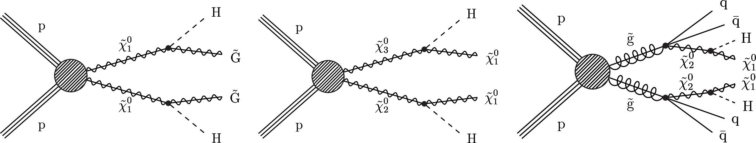
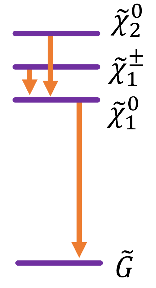
png pdf	Figure 1: Diagrams for (left) the TChiHH-G signal model, $\tilde{\chi}^0_1 \tilde{\chi}^0_1 \to \mathrm{H} \mathrm{H} \tilde{\mathrm{G}} \tilde{\mathrm{G}} $, in which the $\tilde{\chi}^0_1$ NLSPs are produced indirectly through the cascade decays of several combinations of neutralinos and charginos, as described in the text; (center) TChiHH, in which the electroweak production of two neutralinos leads to two Higgs bosons and two neutralinos ($\tilde{\chi}^0_1 $); (right) T5HH, the strong production of a pair of gluinos, each of which decays via a three-body process to quarks and a neutralino, with the neutralino subsequently decaying to a Higgs boson and a $\tilde{\chi}^0_1$ LSP. In each diagram, the hatched circle represents the sum of processes that can lead to the SUSY particles shown.
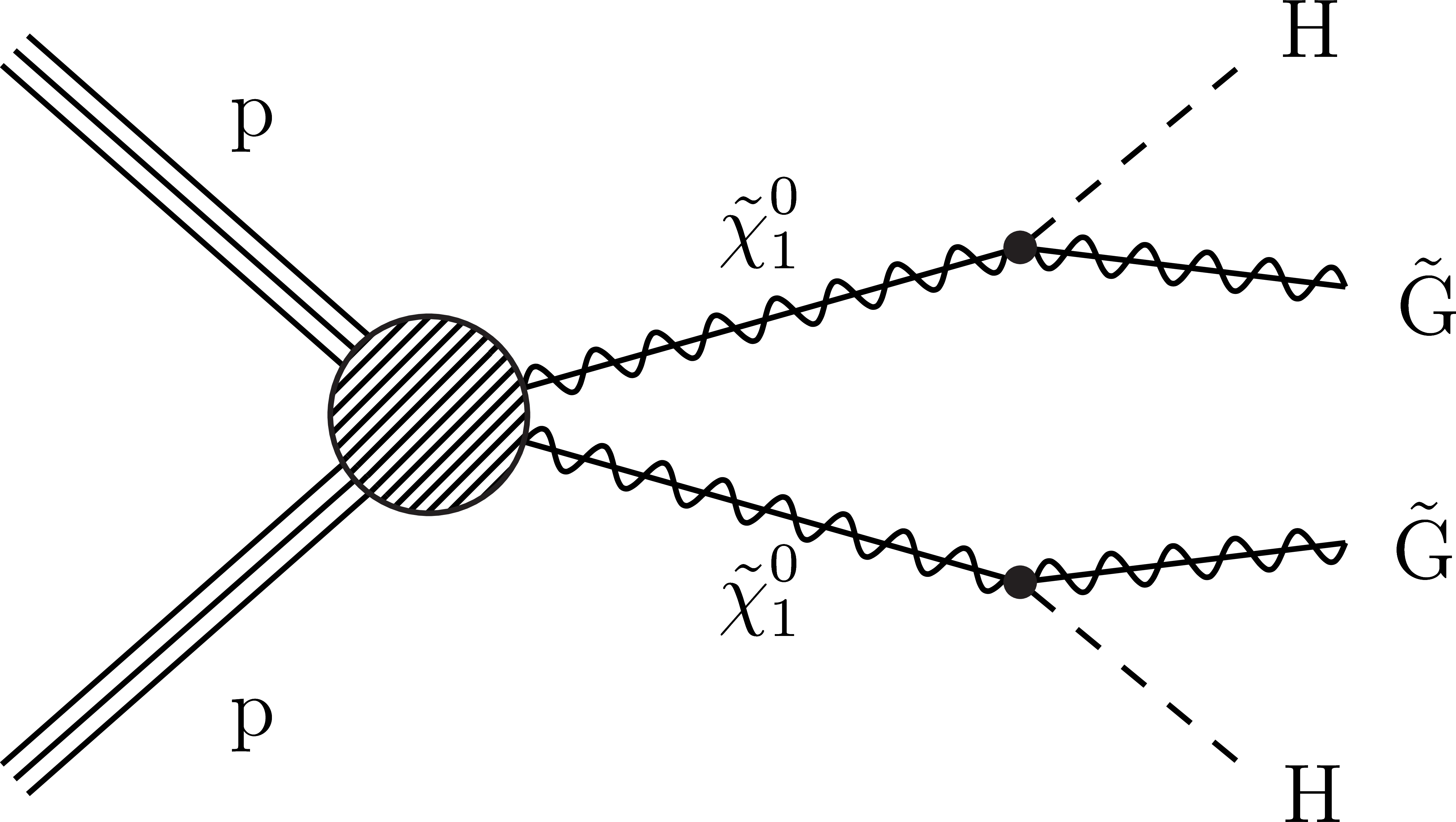
png pdf	Figure 1-a: Diagram for the TChiHH-G signal model, $\tilde{\chi}^0_1 \tilde{\chi}^0_1 \to \mathrm{H} \mathrm{H} \tilde{\mathrm{G}} \tilde{\mathrm{G}} $, in which the $\tilde{\chi}^0_1$ NLSPs are produced indirectly through the cascade decays of several combinations of neutralinos and charginos, as described in the text. The hatched circle represents the sum of processes that can lead to the SUSY particles shown.
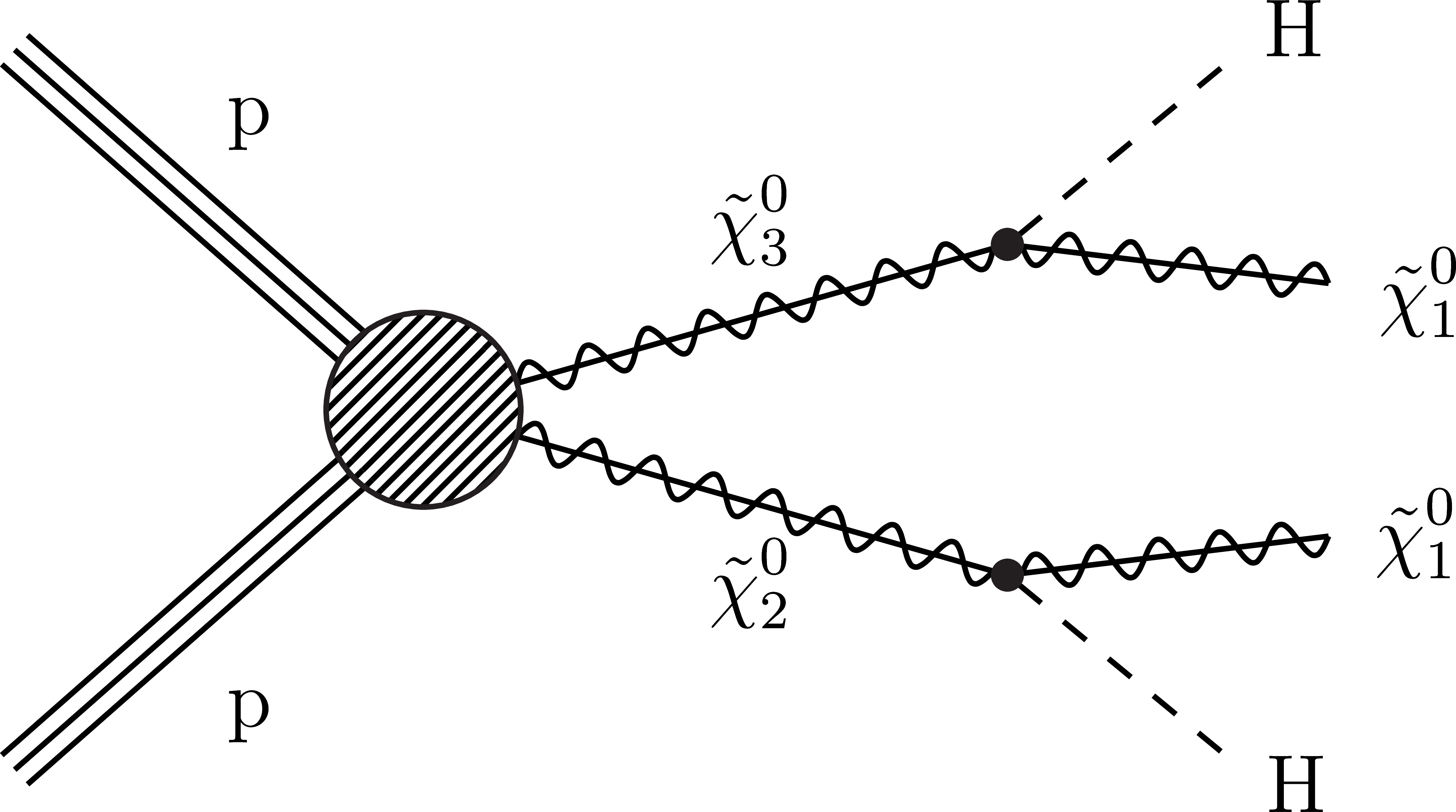
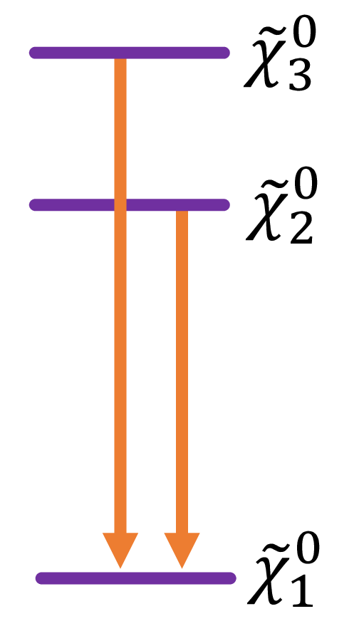
png pdf	Figure 1-b: Diagram for TChiHH, in which the electroweak production of two neutralinos leads to two Higgs bosons and two neutralinos ($\tilde{\chi}^0_1 $). The hatched circle represents the sum of processes that can lead to the SUSY particles shown.
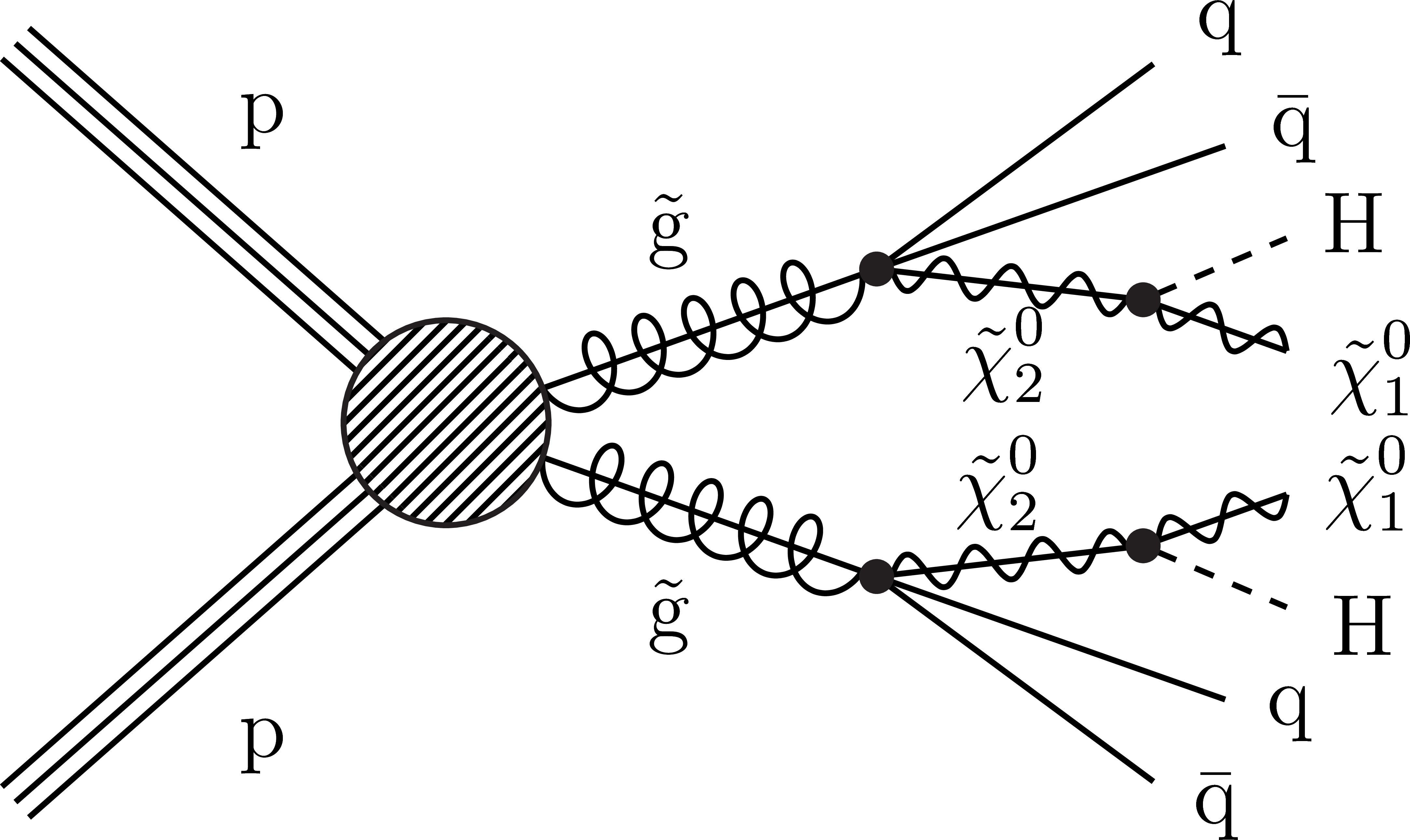
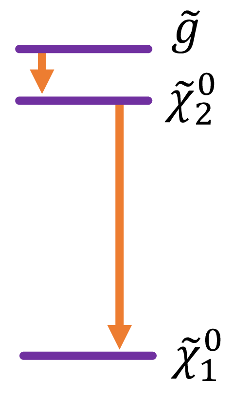
png pdf	Figure 1-c: Diagram for T5HH, the strong production of a pair of gluinos, each of which decays via a three-body process to quarks and a neutralino, with the neutralino subsequently decaying to a Higgs boson and a $\tilde{\chi}^0_1$ LSP. The hatched circle represents the sum of processes that can lead to the SUSY particles shown.
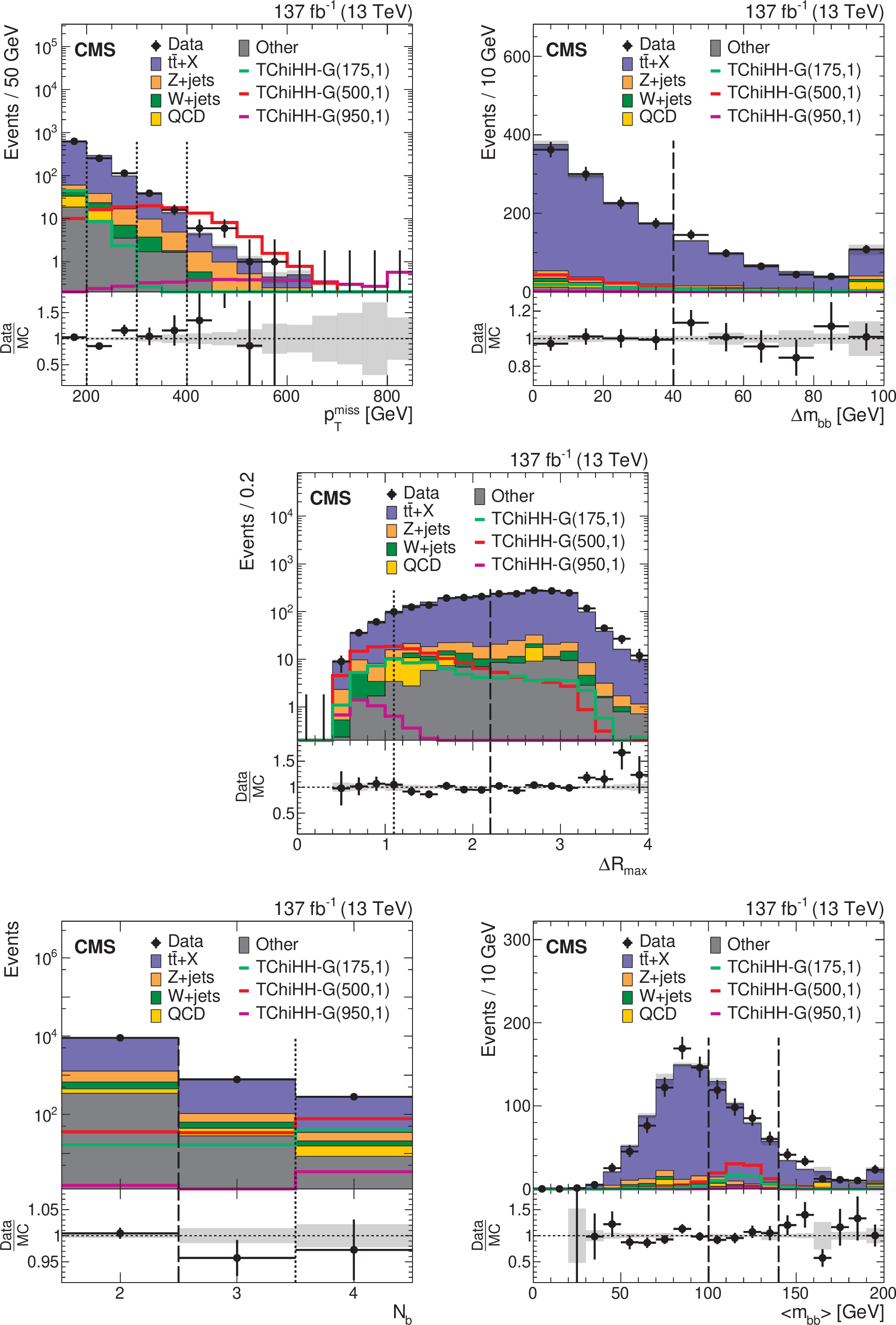
png pdf	Figure 2: Distributions in key analysis variables of the resolved signature for events satisfying the baseline requirements and $ {N_\mathrm{b}} =$ 3 or 4, except for those on the variable plotted: (upper left) ${{p_{\mathrm {T}}} ^\text {miss}}$, (upper right) ${\Delta m_{\mathrm{b} \mathrm{b}}}$, (middle) ${\Delta R_{\text {max}}}$, (lower left) ${N_\mathrm{b}}$, and (lower right) ${< m_{\mathrm{b} \mathrm{b}}>}$. The rightmost bins include the overflow entries. The data are shown as black markers with error bars, simulated SM backgrounds by the stacked histograms (scaled by factors of 0.93-0.97 to match the total data yield in each plot), and simulations of signals TChiHH-G($m(\tilde{\chi}^0_1),m(\tilde{\mathrm{G}}$) [GeV]) by the open colored histograms. Gray shading represents the statistical uncertainties of the simulation. Vertical lines indicate the boundaries for signal region selection (dashed), or for the signal region binning (dotted). The lower panels show the ratio of data to (scaled) simulation.
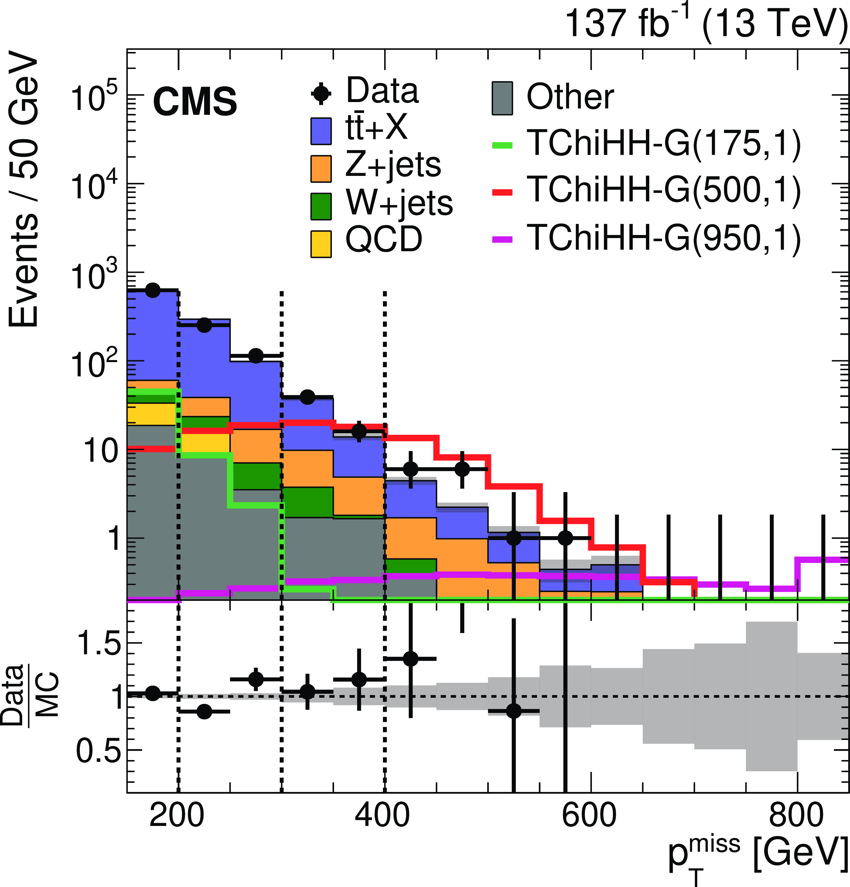
png pdf	Figure 2-a: Distribution of ${{p_{\mathrm {T}}} ^\text {miss}}$ for events satisfying the baseline requirements and $ {N_\mathrm{b}} =$ 3 or 4. The rightmost bins includes the overflow entries. The data are shown as black markers with error bars, simulated SM backgrounds by the stacked histograms (scaled by a factor to match the total data yield), and simulations of signals TChiHH-G($m(\tilde{\chi}^0_1),m(\tilde{\mathrm{G}}$) [GeV]) by the open colored histograms. Gray shading represents the statistical uncertainties of the simulation. Vertical lines indicate the boundaries for signal region selection (dashed), or for the signal region binning (dotted). The lower panel shows the ratio of data to (scaled) simulation.
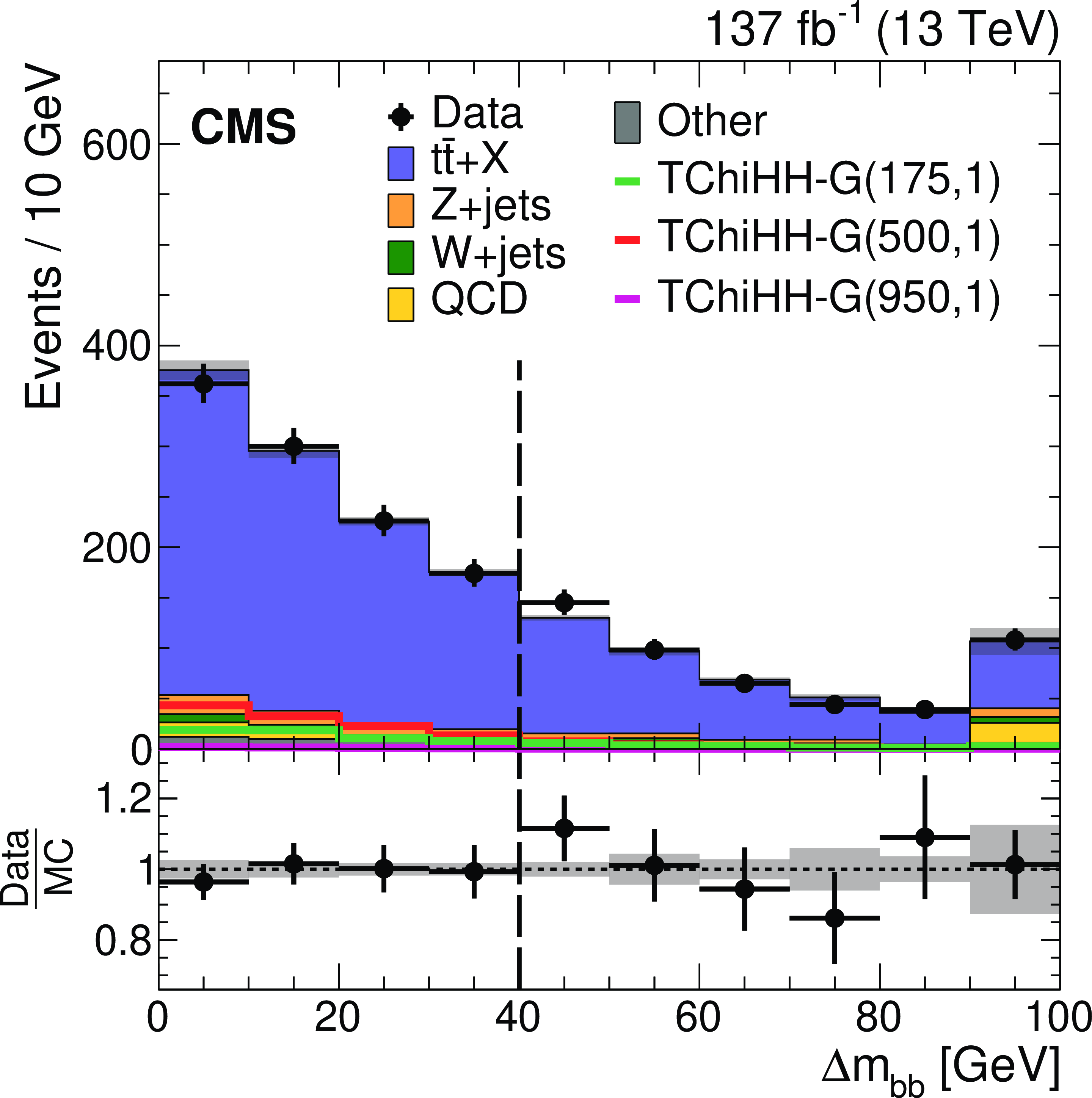
png pdf	Figure 2-b: Distribution of ${\Delta m_{\mathrm{b} \mathrm{b}}}$ for events satisfying the baseline requirements and $ {N_\mathrm{b}} =$ 3 or 4. The rightmost bins includes the overflow entries. The data are shown as black markers with error bars, simulated SM backgrounds by the stacked histograms (scaled by a factor to match the total data yield), and simulations of signals TChiHH-G($m(\tilde{\chi}^0_1),m(\tilde{\mathrm{G}}$) [GeV]) by the open colored histograms. Gray shading represents the statistical uncertainties of the simulation. Vertical lines indicate the boundaries for signal region selection (dashed), or for the signal region binning (dotted). The lower panel shows the ratio of data to (scaled) simulation.
png pdf	Figure 2-c: Distribution of ${\Delta R_{\text {max}}}$ for events satisfying the baseline requirements and $ {N_\mathrm{b}} =$ 3 or 4. The rightmost bins includes the overflow entries. The data are shown as black markers with error bars, simulated SM backgrounds by the stacked histograms (scaled by a factor to match the total data yield), and simulations of signals TChiHH-G($m(\tilde{\chi}^0_1),m(\tilde{\mathrm{G}}$) [GeV]) by the open colored histograms. Gray shading represents the statistical uncertainties of the simulation. Vertical lines indicate the boundaries for signal region selection (dashed), or for the signal region binning (dotted). The lower panel shows the ratio of data to (scaled) simulation.
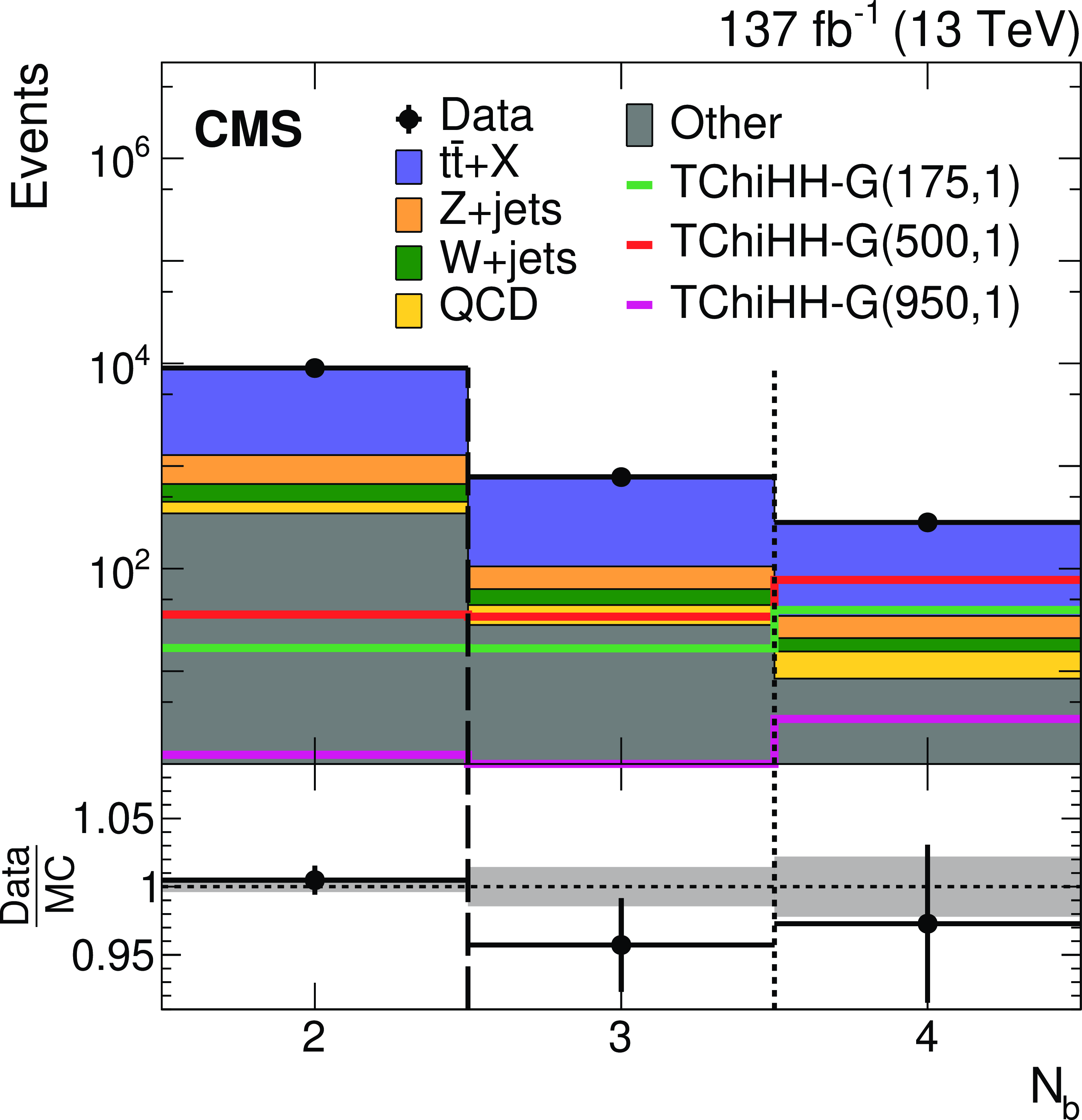
png pdf	Figure 2-d: Distribution of ${N_\mathrm{b}}$ for events satisfying the baseline requirements and $ {N_\mathrm{b}} =$ 3 or 4. The rightmost bins includes the overflow entries. The data are shown as black markers with error bars, simulated SM backgrounds by the stacked histograms (scaled by a factor to match the total data yield), and simulations of signals TChiHH-G($m(\tilde{\chi}^0_1),m(\tilde{\mathrm{G}}$) [GeV]) by the open colored histograms. Gray shading represents the statistical uncertainties of the simulation. Vertical lines indicate the boundaries for signal region selection (dashed), or for the signal region binning (dotted). The lower panel shows the ratio of data to (scaled) simulation.
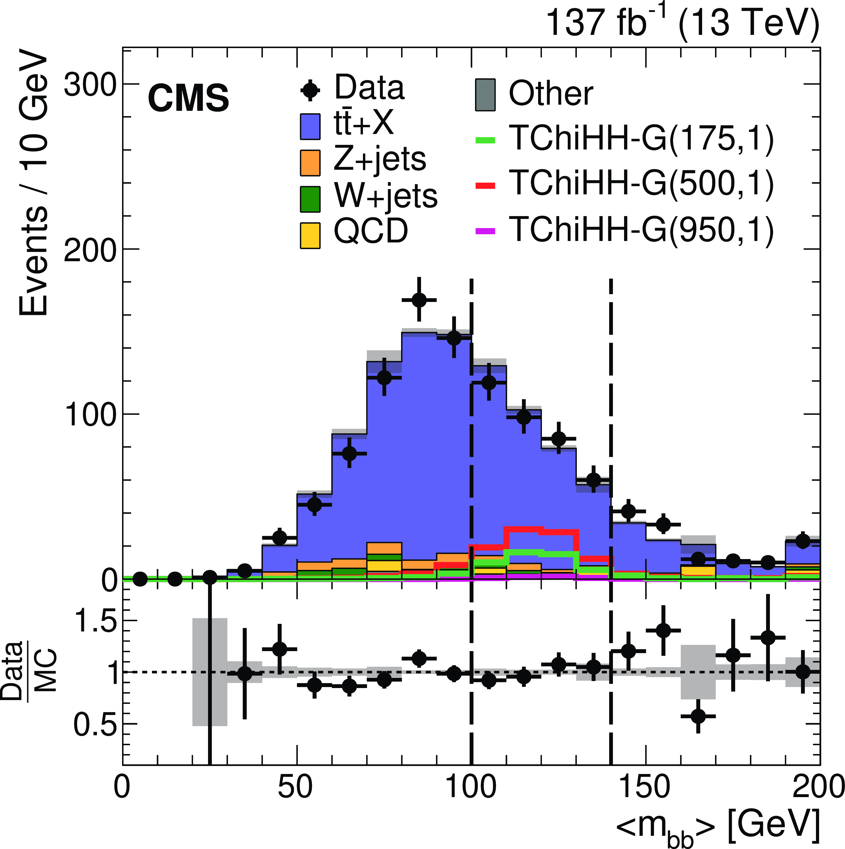
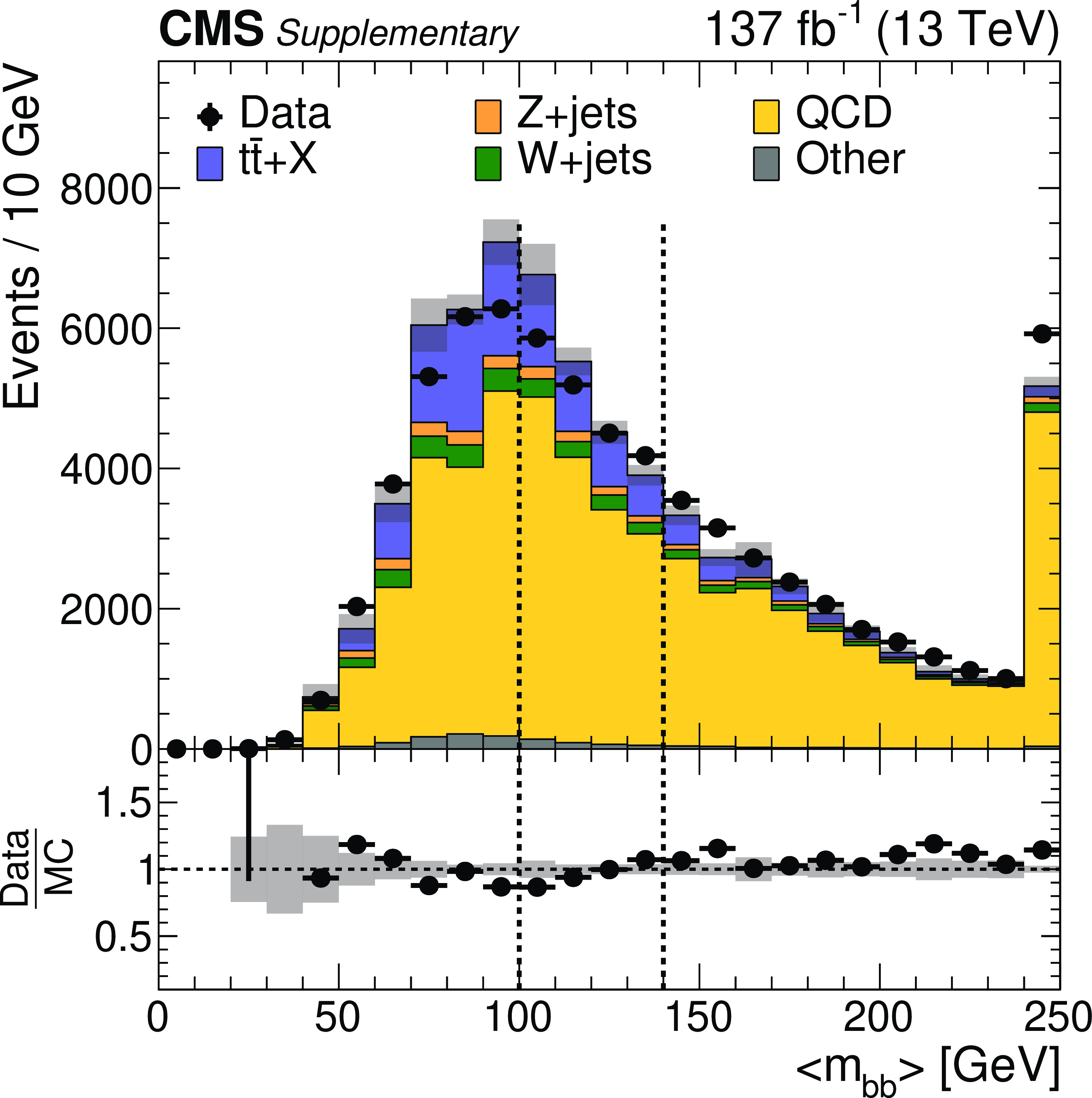
png pdf	Figure 2-e: Distributions of ${< m_{\mathrm{b} \mathrm{b}}>}$ for events satisfying the baseline requirements and $ {N_\mathrm{b}} =$ 3 or 4. The rightmost bins includes the overflow entries. The data are shown as black markers with error bars, simulated SM backgrounds by the stacked histograms (scaled by a factor to match the total data yield), and simulations of signals TChiHH-G($m(\tilde{\chi}^0_1),m(\tilde{\mathrm{G}}$) [GeV]) by the open colored histograms. Gray shading represents the statistical uncertainties of the simulation. Vertical lines indicate the boundaries for signal region selection (dashed), or for the signal region binning (dotted). The lower panel shows the ratio of data to (scaled) simulation.
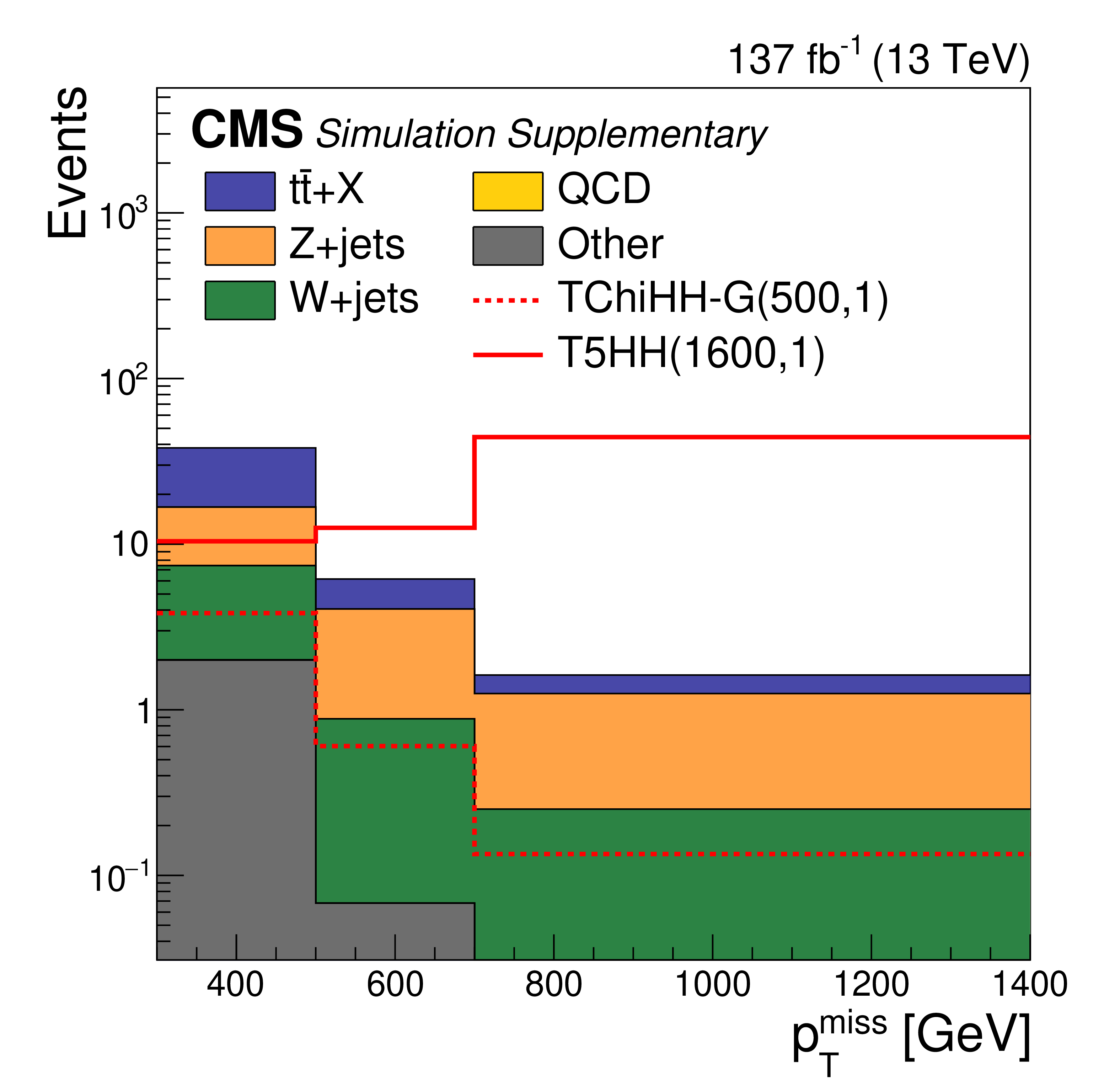
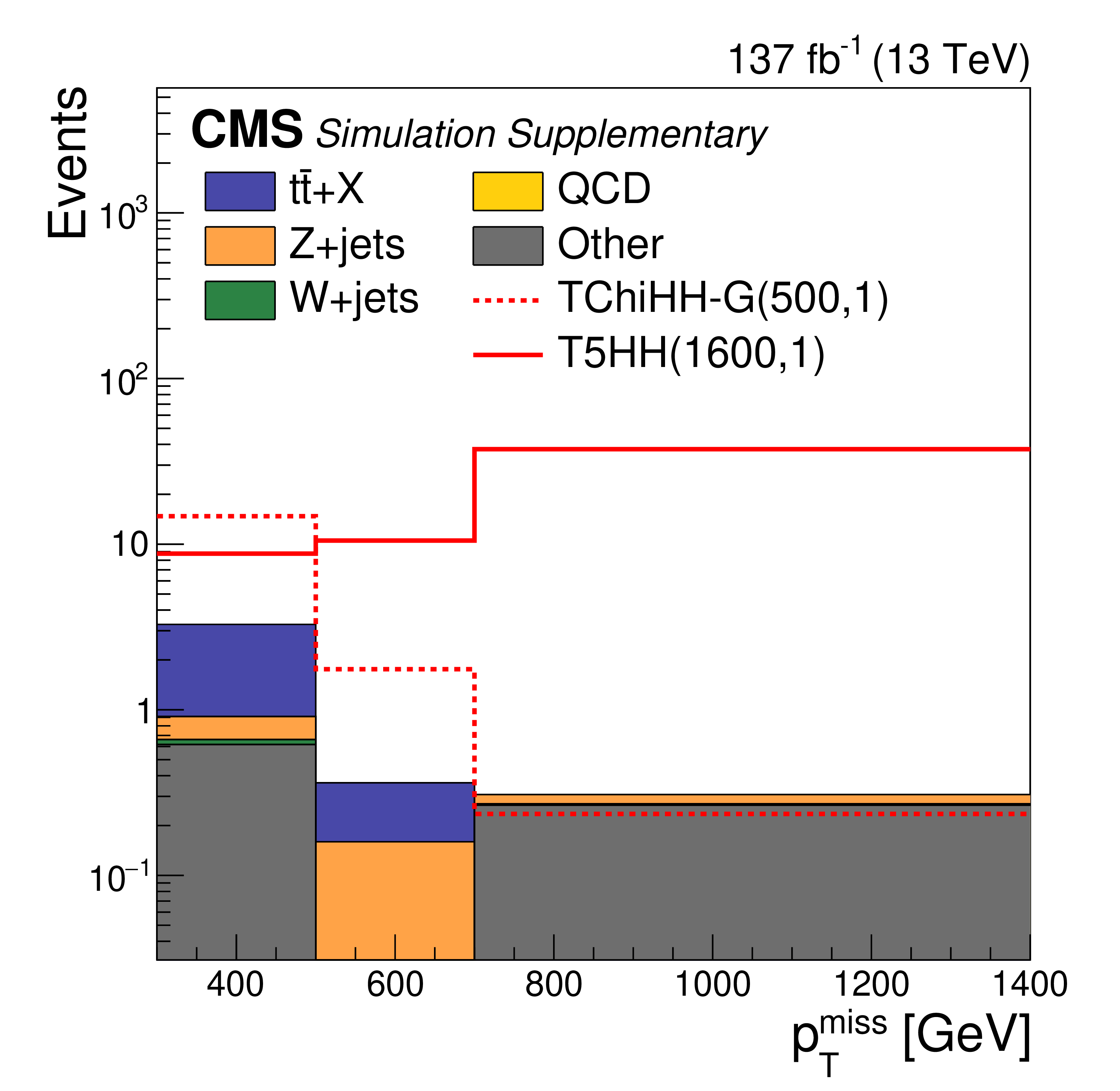
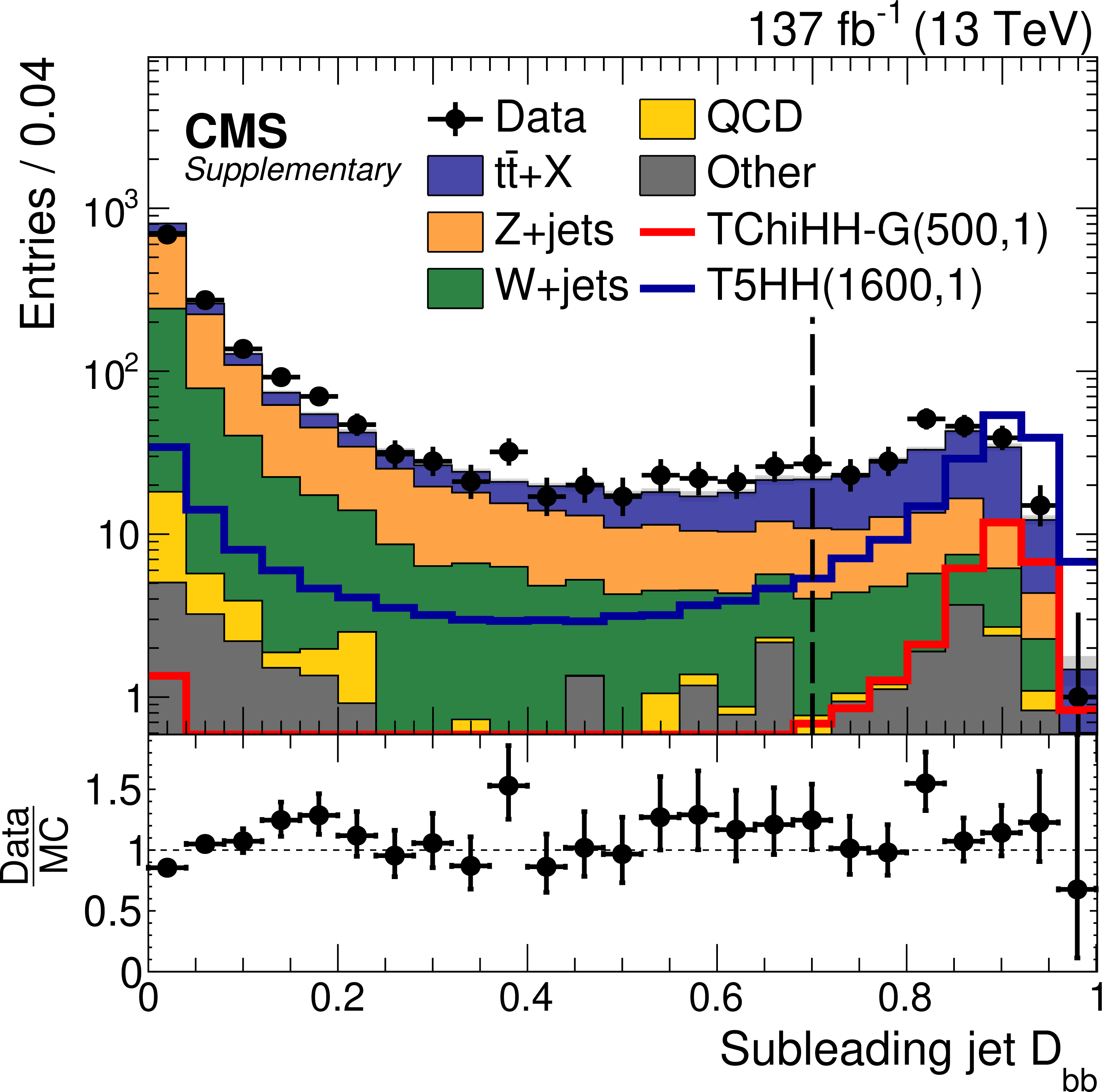
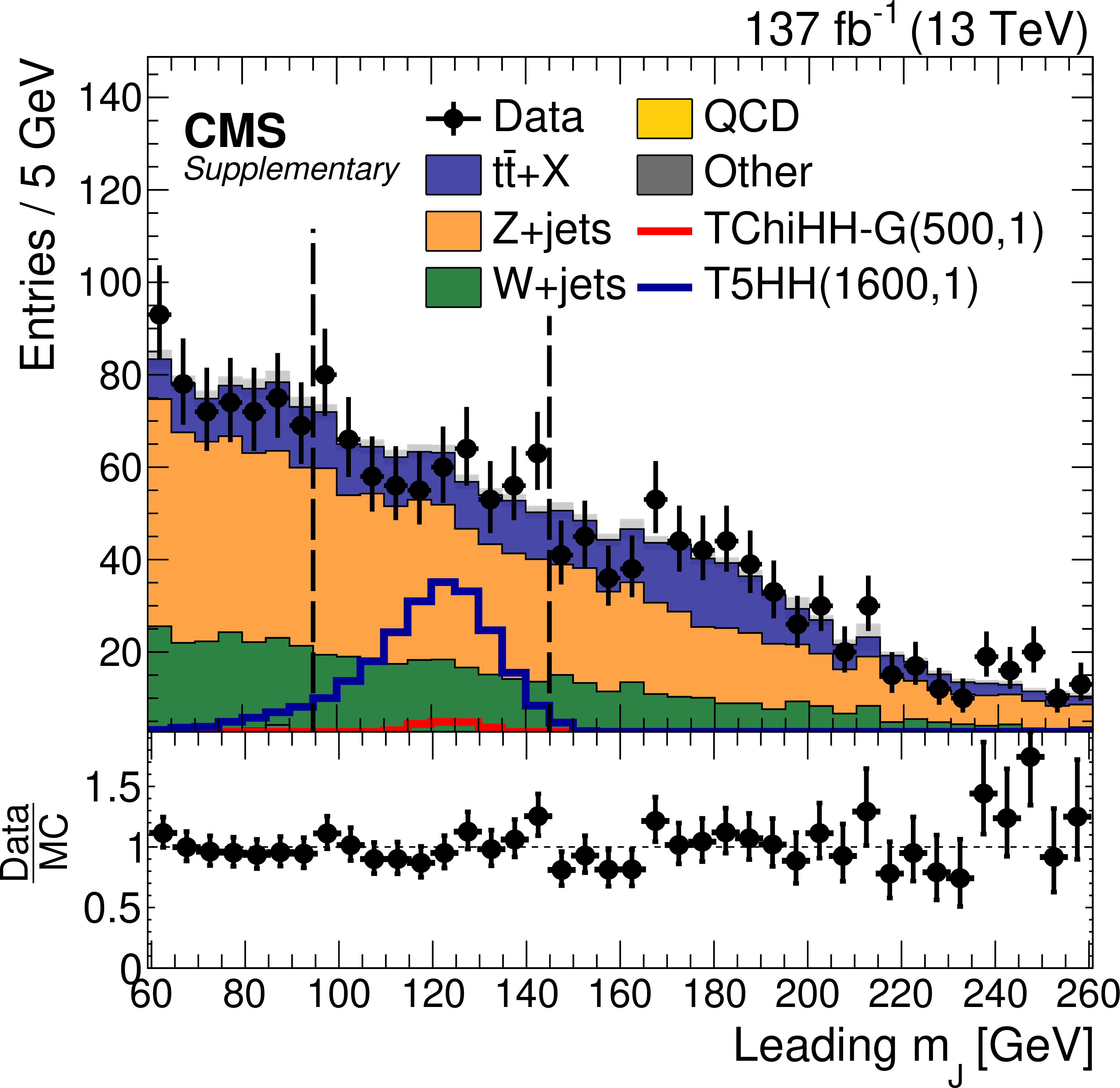
png pdf	Figure 3: Distributions in key analysis variables after the baseline requirements for the boosted signature, except for those on the variable plotted: (upper left) ${{p_{\mathrm {T}}} ^\text {miss}}$, (upper right) jet ${p_{\mathrm {T}}}$, (lower left) ${D_{ {\mathrm{b} \mathrm{b}}}}$, and (lower right) ${m_{\mathrm {J}}}$. Except for the ${{p_{\mathrm {T}}} ^\text {miss}}$ distribution, each plot contains two entries per event, for each of the two ${p_{\mathrm {T}}}$-leading AK8 jets. The data are shown by the black markers with error bars, and SM backgrounds from simulation (scaled by 86% to match the data integral) by the filled histograms. Open colored histograms show simulations of the signals TChiHH-G($m(\tilde{\chi}^0_1)$, $m(\tilde{\mathrm{G}})$) or T5HH($m({\mathrm{\widetilde{g}}})$, $m(\tilde{\chi}^0_1$)[GeV]). The vertical dashed lines show boundaries for the event classifications defined in Section 7: (upper left) the ${{p_{\mathrm {T}}} ^\text {miss}}$ binning; (lower left) the ${D_{ {\mathrm{b} \mathrm{b}}}}$ threshold for identification of a jet as an ${\mathrm{H} \to \mathrm{b} \mathrm{\bar{b}}}$ candidate; (lower right) the boundaries of the H boson mass window. The lower panel in each plot shows the ratio of observed to (scaled) simulated yields.
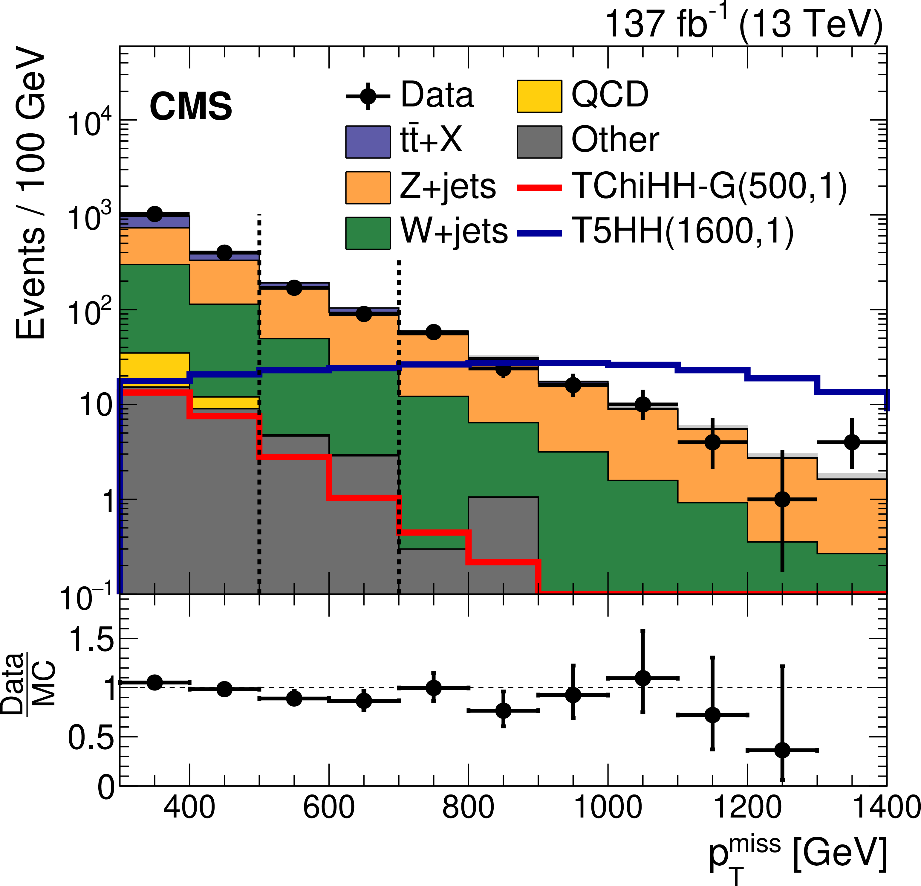
png pdf	Figure 3-a: Distribution of ${{p_{\mathrm {T}}} ^\text {miss}}$ after the baseline requirements for the boosted signature. The data are shown by the black markers with error bars, and SM backgrounds from simulation (scaled by 86% to match the data integral) by the filled histograms. Open colored histograms show simulations of the signals TChiHH-G($m(\tilde{\chi}^0_1)$, $m(\tilde{\mathrm{G}})$) or T5HH($m({\mathrm{\widetilde{g}}})$, $m(\tilde{\chi}^0_1$)[GeV]). The vertical dashed lines show the ${{p_{\mathrm {T}}} ^\text {miss}}$ binning. The lower panel shows the ratio of observed to (scaled) simulated yields.
png pdf	Figure 3-b: Distribution of jet ${p_{\mathrm {T}}}$ after the baseline requirements for the boosted signature, except for those on the variable plotted. The plot contains two entries per event, for each of the two ${p_{\mathrm {T}}}$-leading AK8 jets. The data are shown by the black markers with error bars, and SM backgrounds from simulation (scaled by 86% to match the data integral) by the filled histograms. Open colored histograms show simulations of the signals TChiHH-G($m(\tilde{\chi}^0_1)$, $m(\tilde{\mathrm{G}})$) or T5HH($m({\mathrm{\widetilde{g}}})$, $m(\tilde{\chi}^0_1$)[GeV]). The lower panel shows the ratio of observed to (scaled) simulated yields.
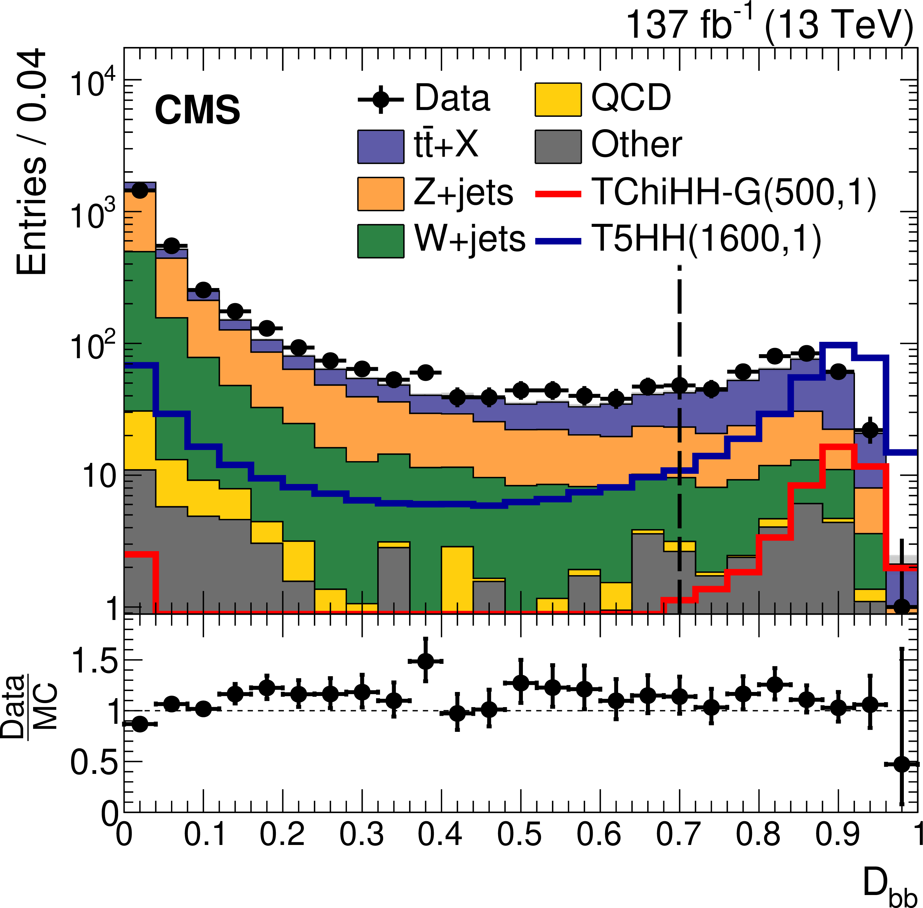
png pdf	Figure 3-c: Distribution of ${D_{ {\mathrm{b} \mathrm{b}}}}$ after the baseline requirements for the boosted signature. The plot contains two entries per event, for each of the two ${p_{\mathrm {T}}}$-leading AK8 jets. The data are shown by the black markers with error bars, and SM backgrounds from simulation (scaled by 86% to match the data integral) by the filled histograms. Open colored histograms show simulations of the signals TChiHH-G($m(\tilde{\chi}^0_1)$, $m(\tilde{\mathrm{G}})$) or T5HH($m({\mathrm{\widetilde{g}}})$, $m(\tilde{\chi}^0_1$)[GeV]). The vertical dashed line shows the ${D_{ {\mathrm{b} \mathrm{b}}}}$ threshold for identification of a jet as an ${\mathrm{H} \to \mathrm{b} \mathrm{\bar{b}}}$ candidate. The lower panel shows the ratio of observed to (scaled) simulated yields.
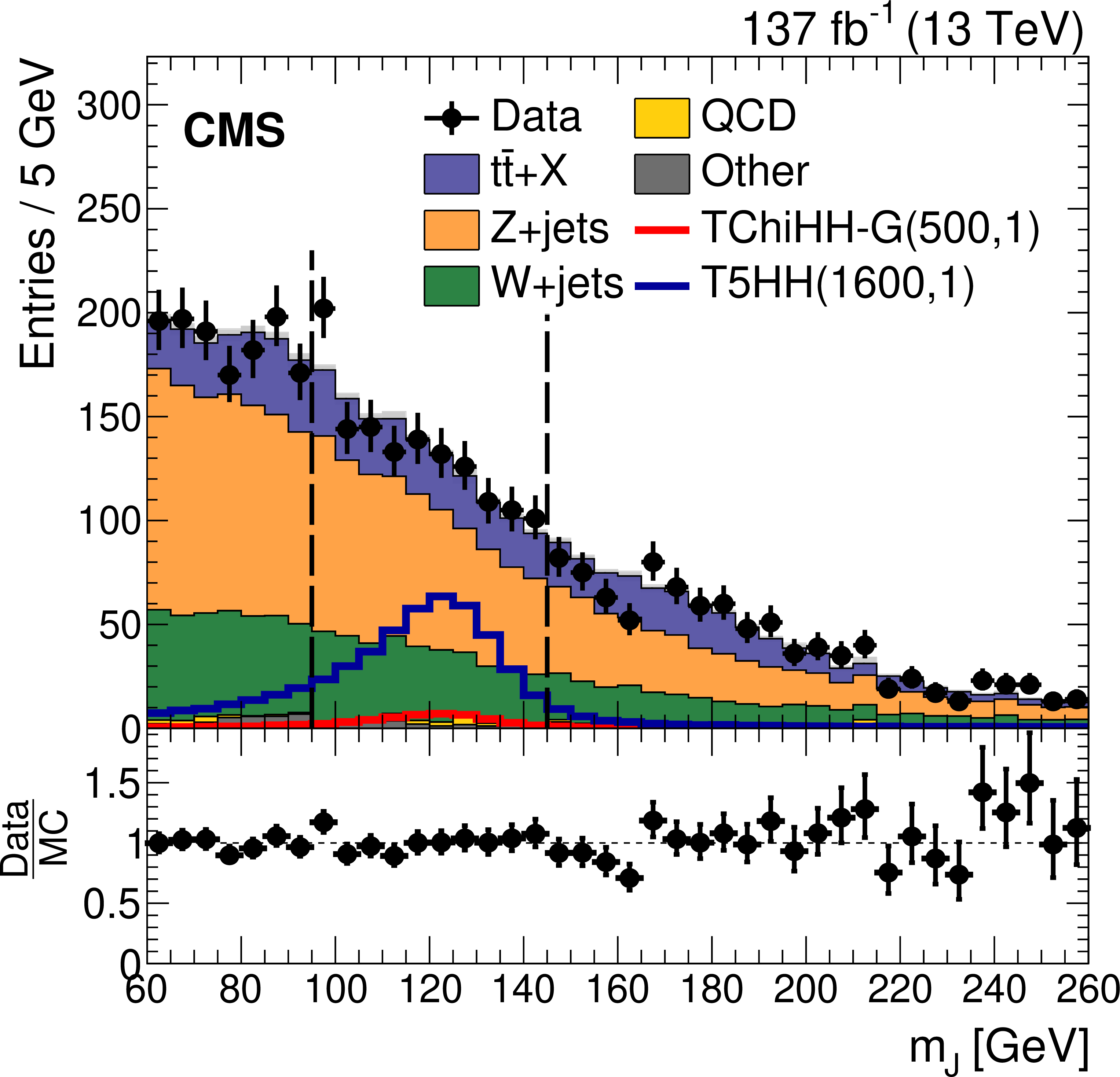
png pdf	Figure 3-d: Distribution of ${m_{\mathrm {J}}}$ after the baseline requirements for the boosted signature. The plot contains two entries per event, for each of the two ${p_{\mathrm {T}}}$-leading AK8 jets. The data are shown by the black markers with error bars, and SM backgrounds from simulation (scaled by 86% to match the data integral) by the filled histograms. Open colored histograms show simulations of the signals TChiHH-G($m(\tilde{\chi}^0_1)$, $m(\tilde{\mathrm{G}})$) or T5HH($m({\mathrm{\widetilde{g}}})$, $m(\tilde{\chi}^0_1$)[GeV]). The vertical dashed lines show the boundaries of the H boson mass window. The lower panel shows the ratio of observed to (scaled) simulated yields.
png pdf	Figure 4: Configuration of the signal and control regions for the (left) resolved and (right) boosted signatures. The patterns shown are repeated in each of several bins in kinematic or topological variables for improved sensitivity, as discussed in the text.
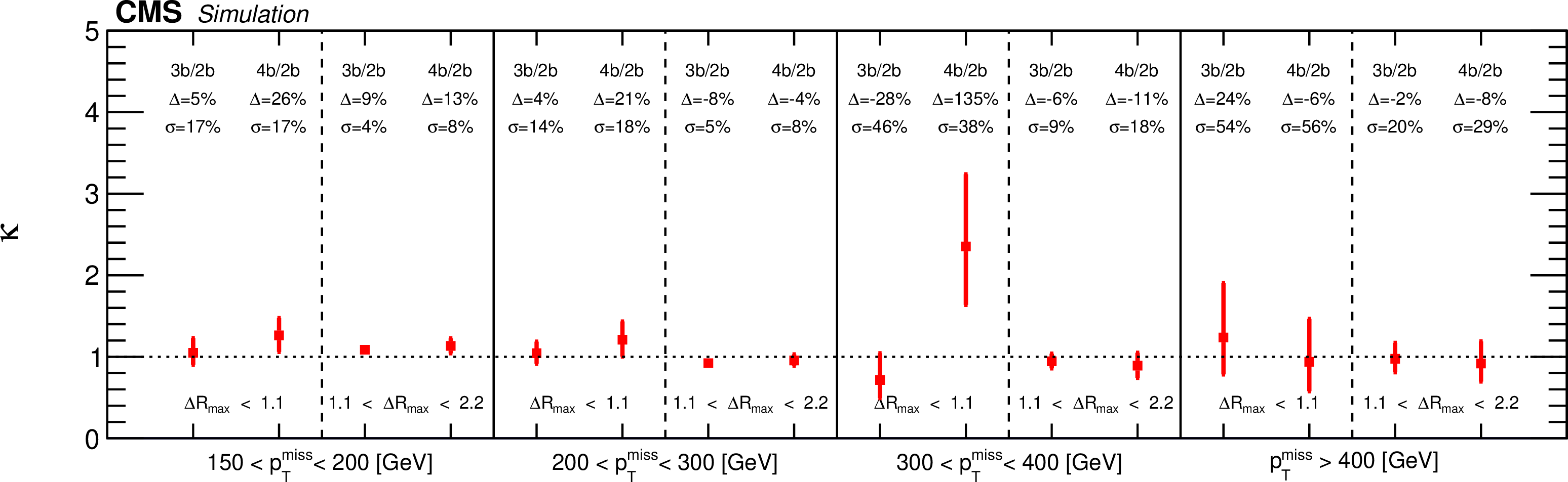
png pdf	Figure 5: The double ratio $\kappa = ({N_{\text {SR}}} / {N_{\text {SB}}})/({N_{\text {CSR}}} / {N_{\text {CSB}}})$ from the SM simulation for the $ {N_\mathrm{b}} =$ 3 and $ {N_\mathrm{b}} =$ 4 search samples for each $({{p_{\mathrm {T}}} ^\text {miss}}$, ${\Delta R_{\text {max}}})$ bin of the resolved signature. The value $\Delta $ gives the deviation of ${\kappa}$ from unity, and $\sigma $ its relative statistical uncertainty.
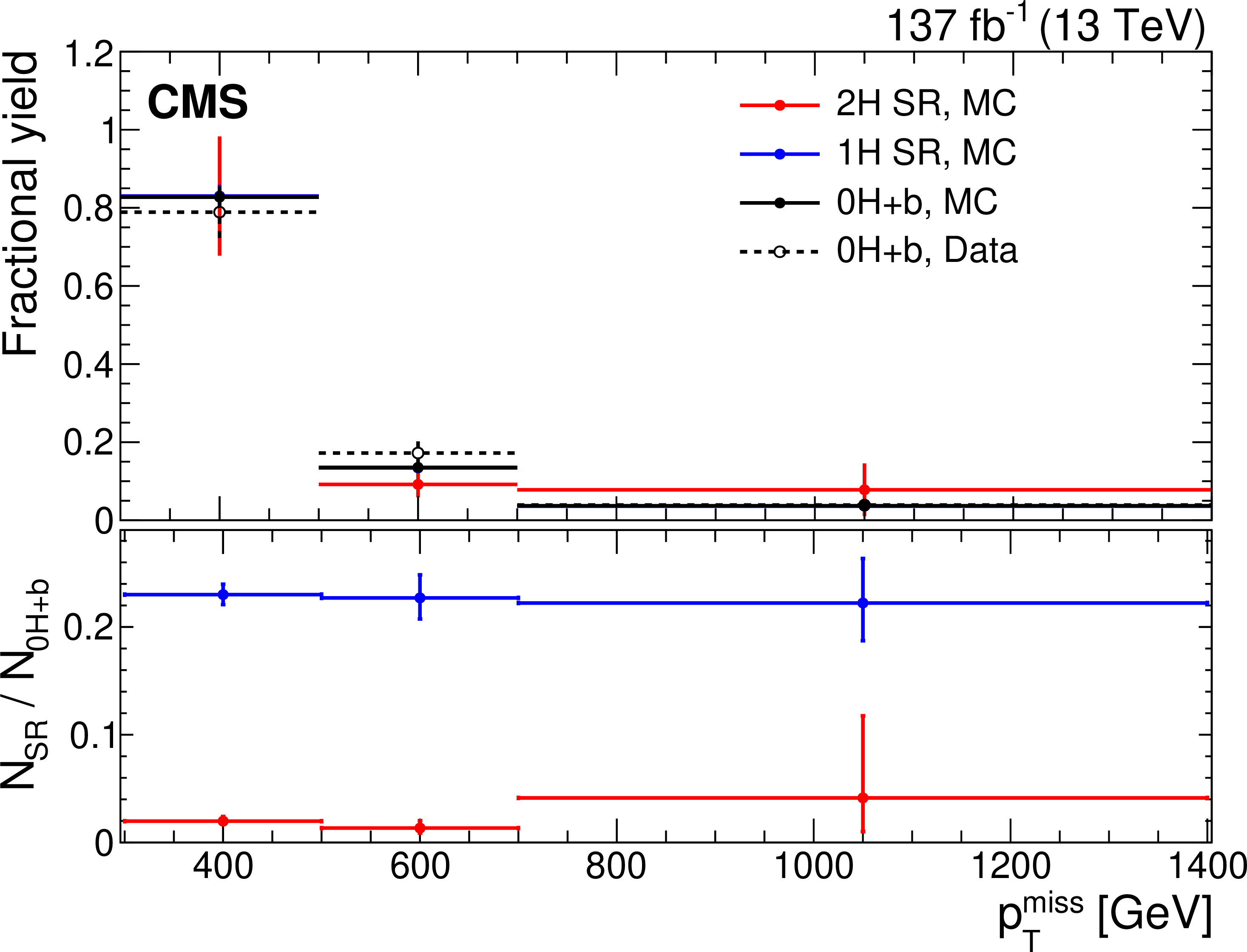
png pdf	Figure 6: (left) The yield ratios $ {N_{\text {CSR}}} / {N_{\text {CSB}}} $ for the 0H region, and $ {N_{\text {SR}}} / {N_{\text {SB}}} $ for 1H and 2H regions of the boosted signature, from the SM simulation. (right) The $ {{p_{\mathrm {T}}} ^\text {miss}} $ distributions of the 2H and 1H SR yields and the 0H+b control region yields, for SM simulation (MC, solid points), and for the control region in data (open black points). In the right-hand plot the upper panel shows the distributions normalized to unit area. The blue points, and in one bin the open point, are hidden under the solid black points. The lower panel shows the (unnormalized) ratios to the 0H+b yields of the 1H (blue) and 2H (red) SR yields, for the simulation. The error bars show the statistical uncertainties.
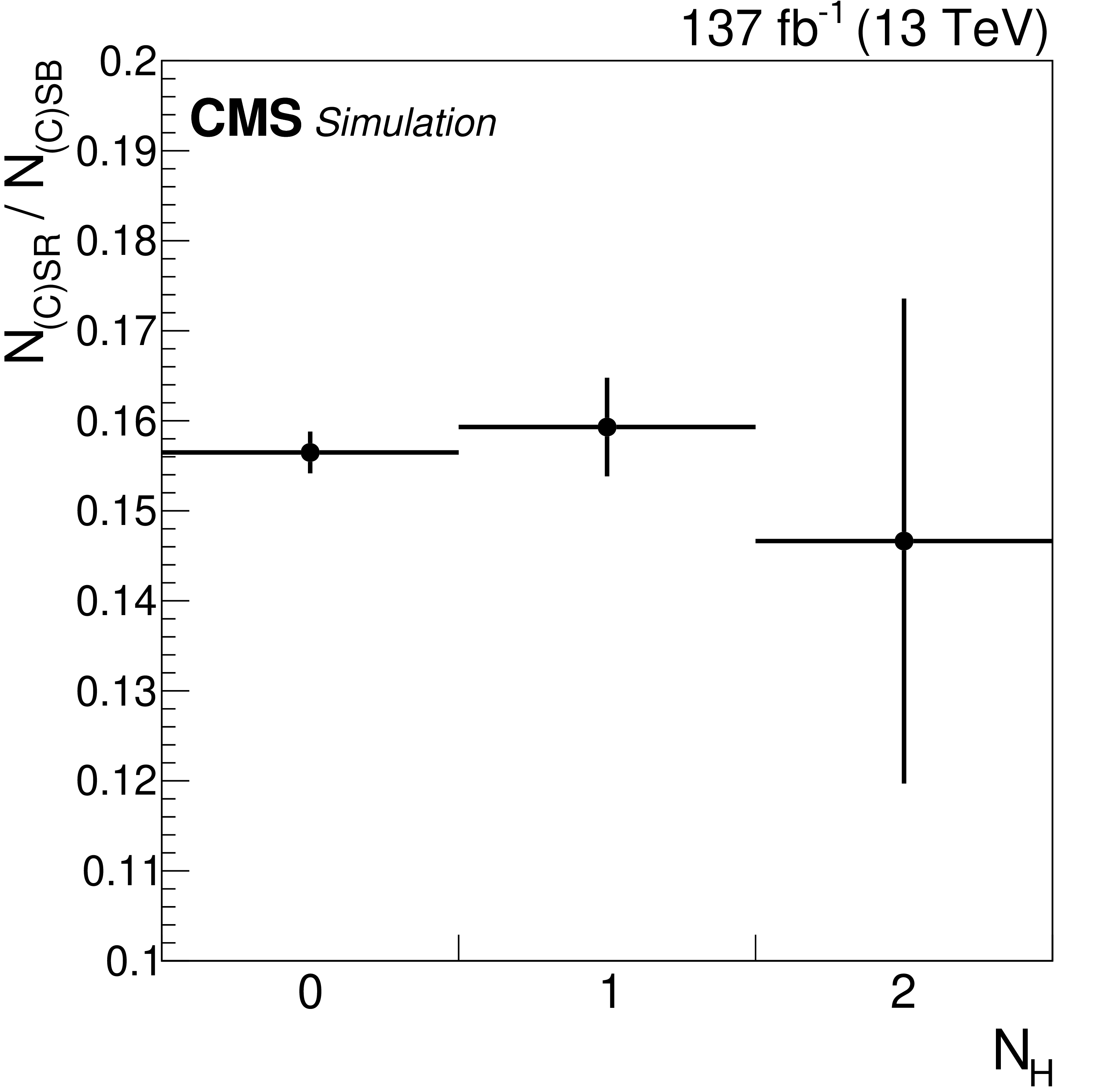
png pdf	Figure 6-a: The yield ratios $ {N_{\text {CSR}}} / {N_{\text {CSB}}} $ for the 0H region, and $ {N_{\text {SR}}} / {N_{\text {SB}}} $ for 1H and 2H regions of the boosted signature, from the SM simulation.
png pdf	Figure 6-b: The $ {{p_{\mathrm {T}}} ^\text {miss}} $ distributions of the 2H and 1H SR yields and the 0H+b control region yields, for SM simulation (MC, solid points), and for the control region in data (open black points). In the right-hand plot the upper panel shows the distributions normalized to unit area. The blue points, and in one bin the open point, are hidden under the solid black points. The lower panel shows the (unnormalized) ratios to the 0H+b yields of the 1H (blue) and 2H (red) SR yields, for the simulation. The error bars show the statistical uncertainties.
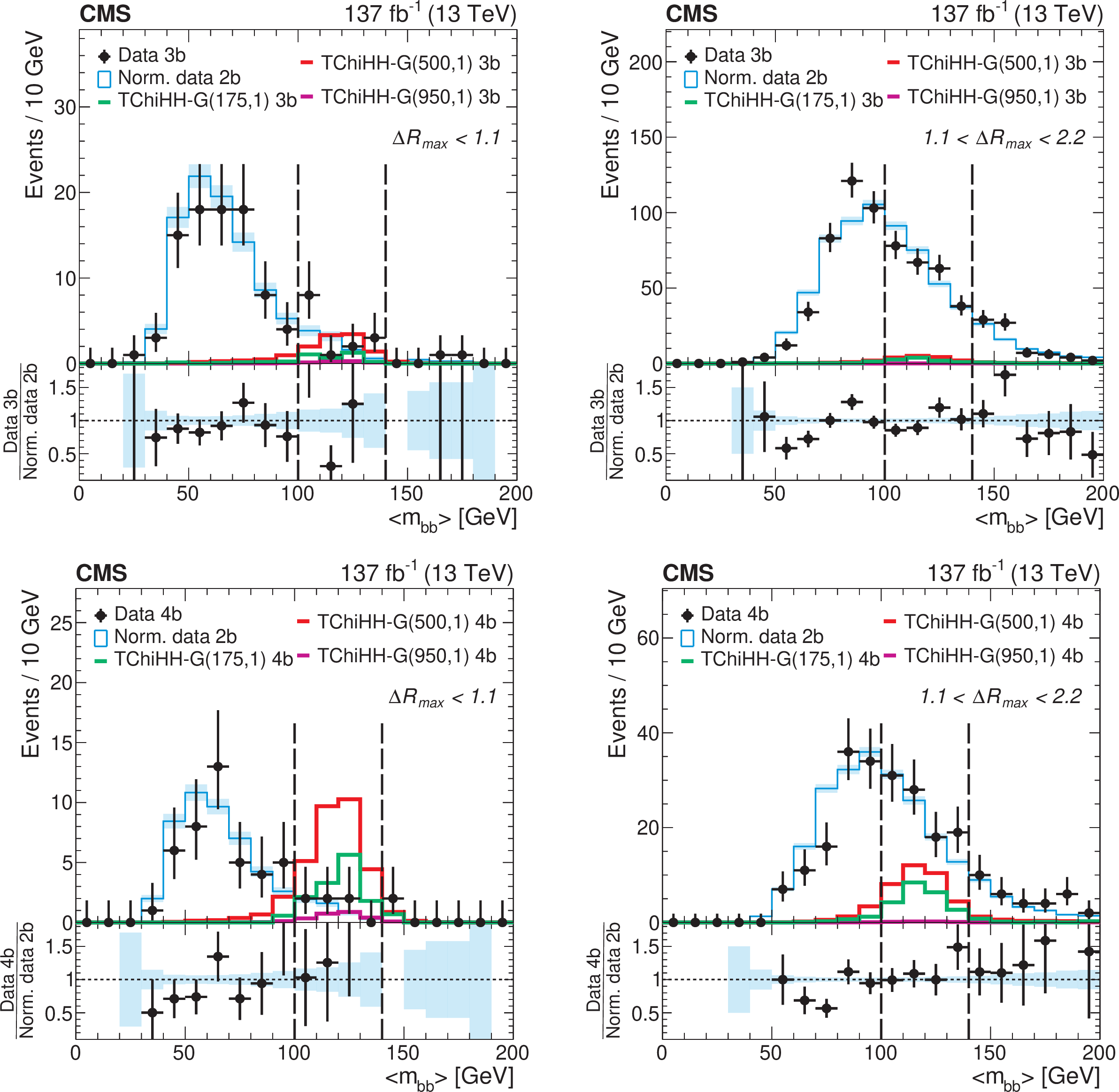
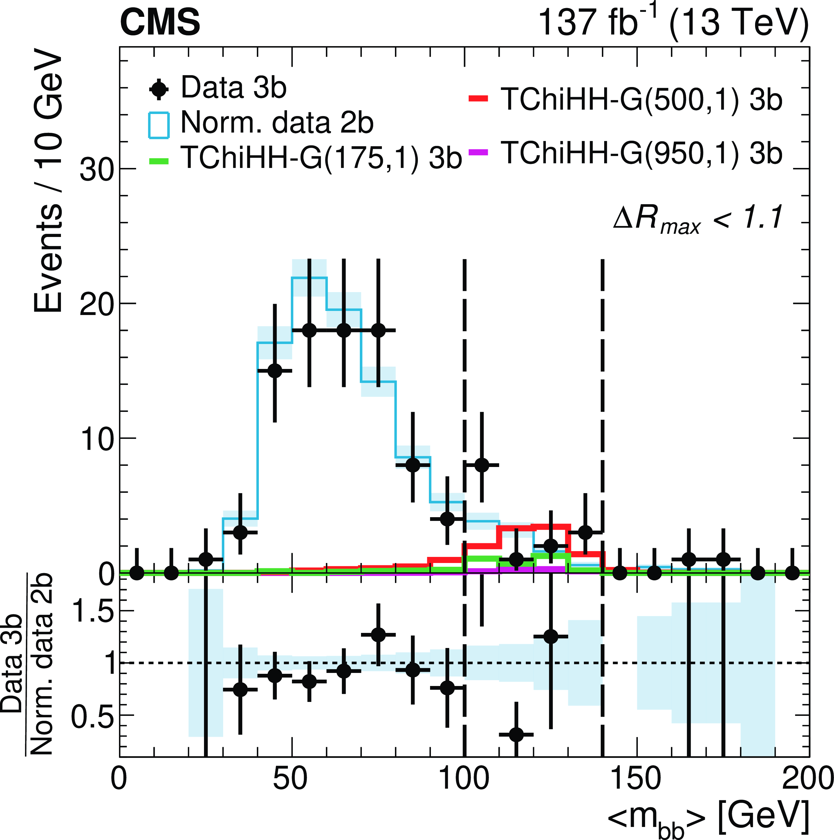
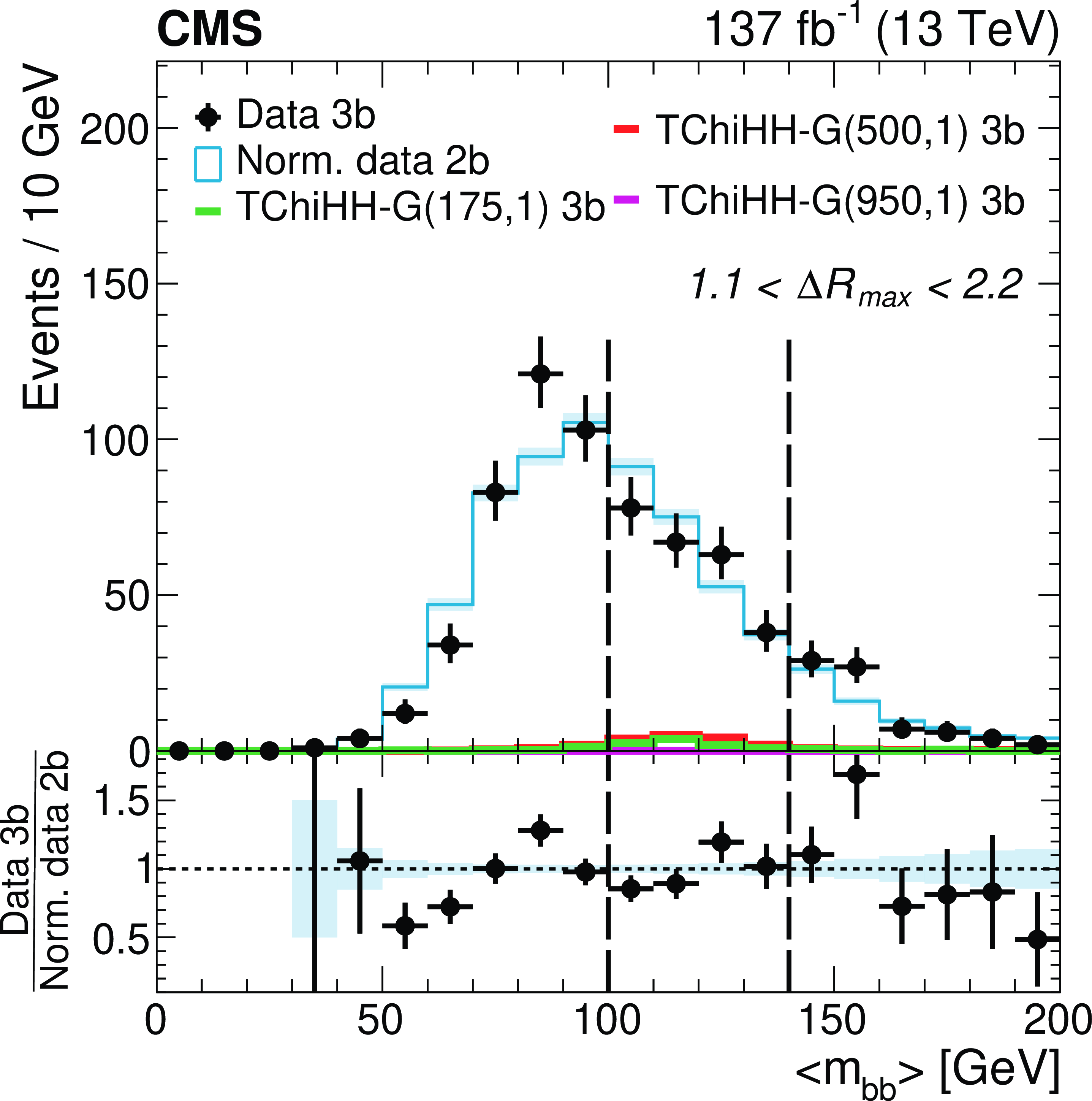
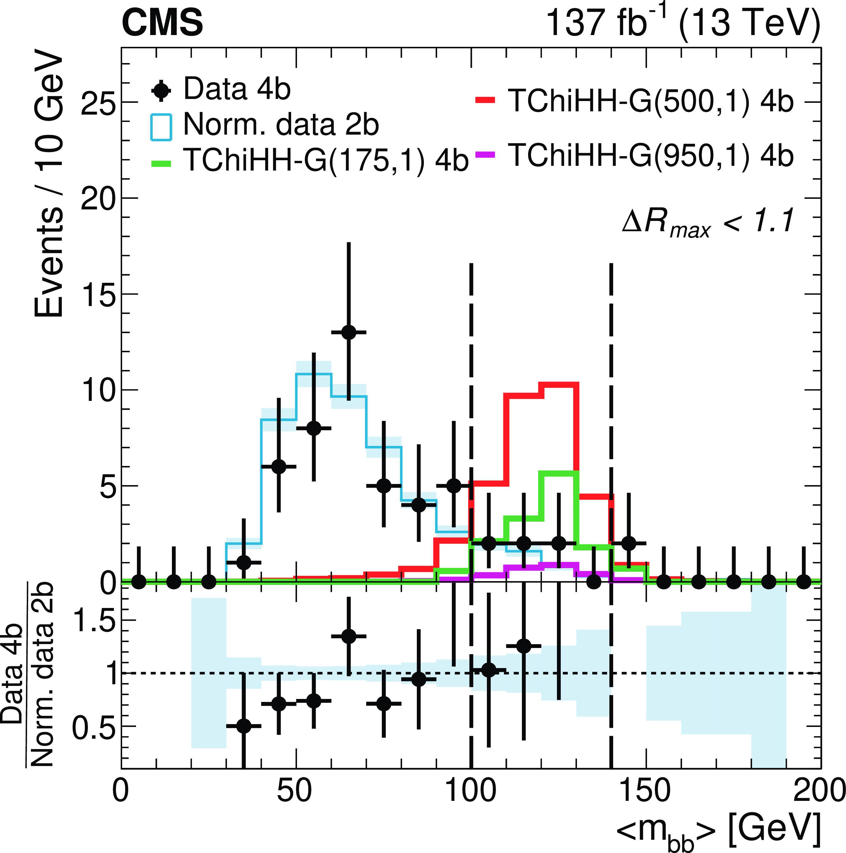
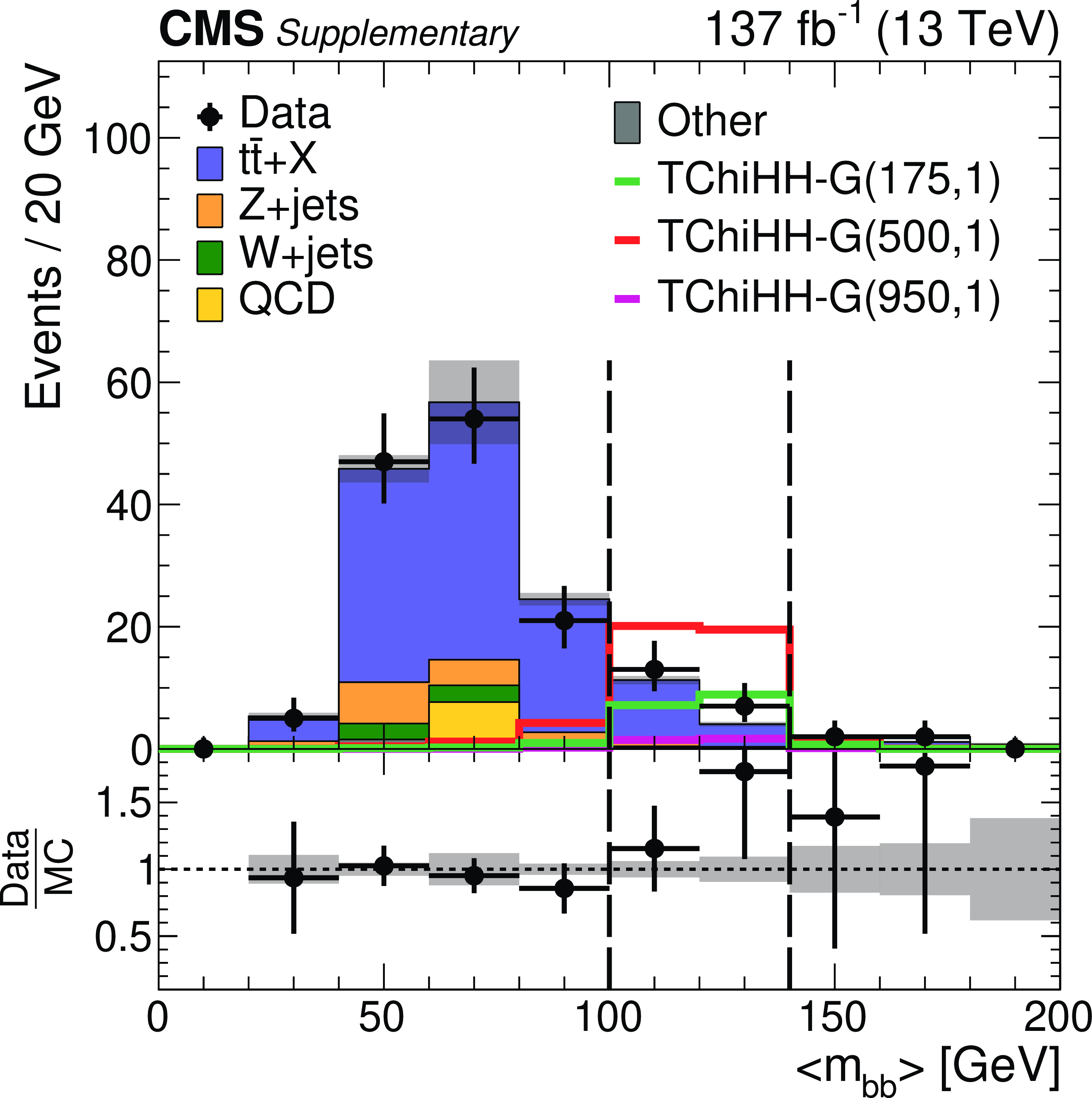
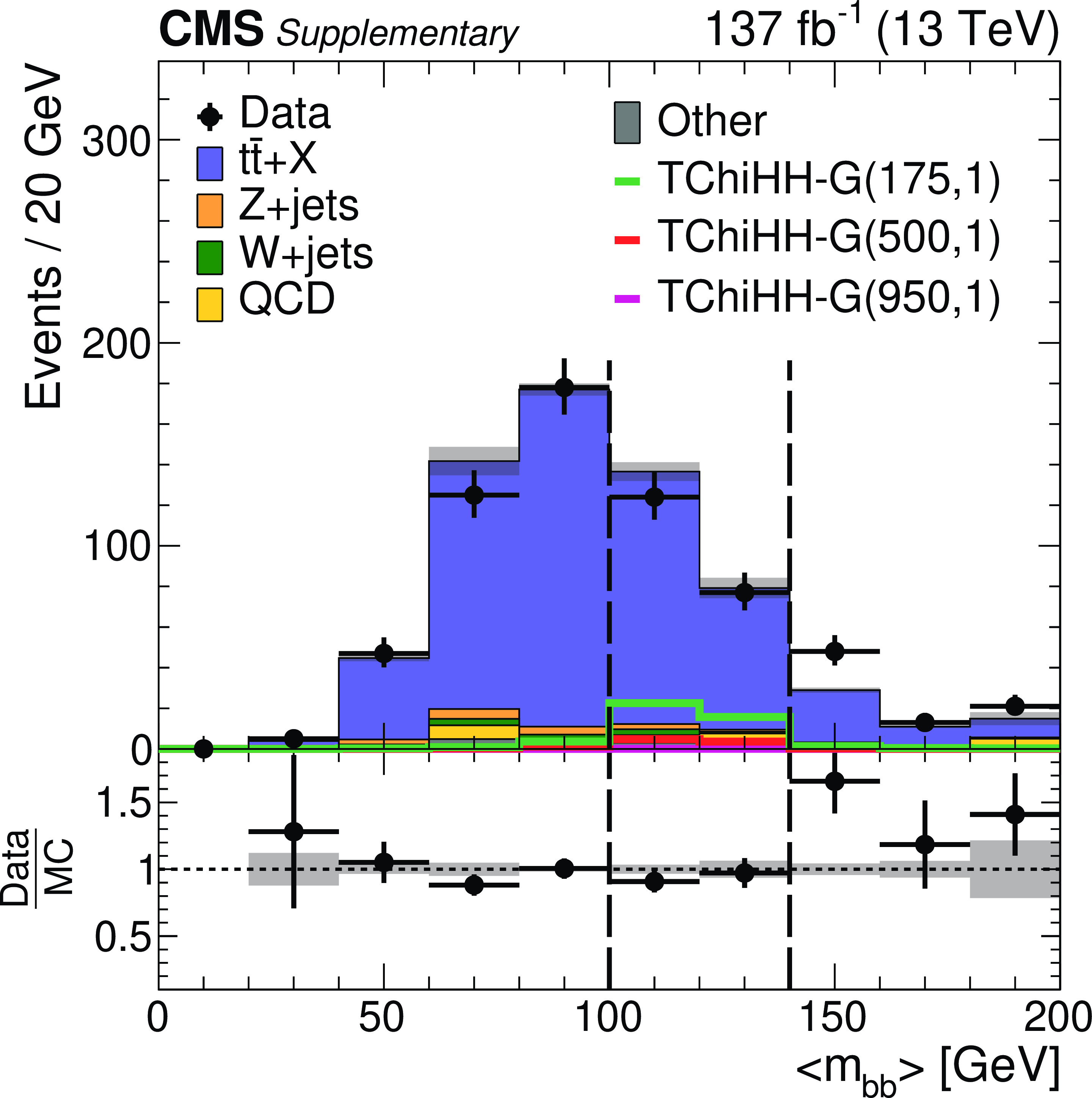
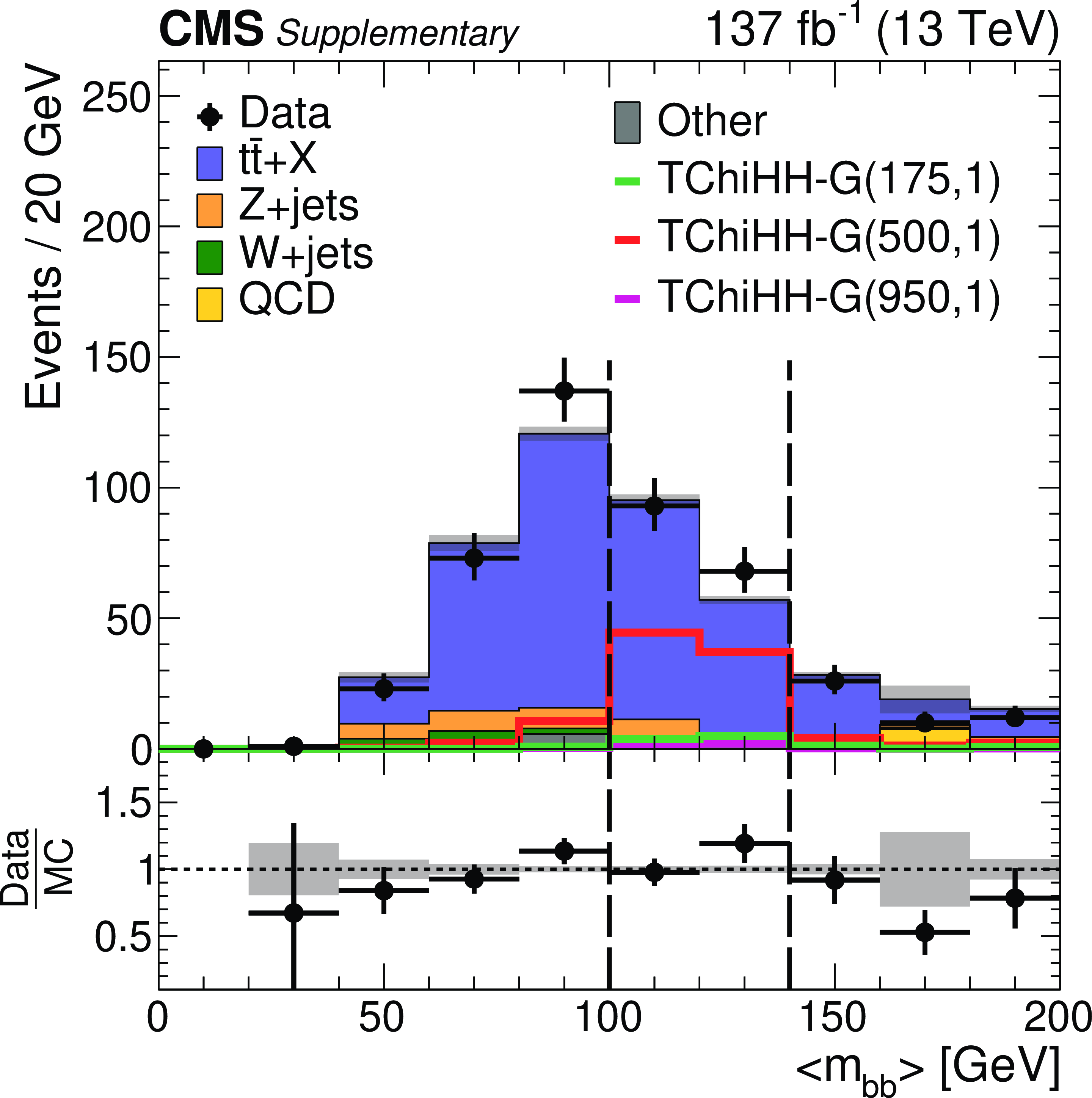
png pdf	Figure 7: Distributions in ${< m_{\mathrm{b} \mathrm{b}}>}$ for the (upper row) $ {N_\mathrm{b}} =$ 3 and (lower row) $ {N_\mathrm{b}} =$ 4 data, denoted by black markers, with error bars indicating the statistical uncertainties. The left-hand set of plots corresponds to $ {\Delta R_{\text {max}}} < $ 1.1, while the right-hand set corresponds to 1.1 $ < {\Delta R_{\text {max}}} < $ 2.2, in both cases integrated over ${{p_{\mathrm {T}}} ^\text {miss}}$. The overlaid cyan histograms show the corresponding distributions of the $ {N_\mathrm{b}} =$ 2 data, reweighted with the appropriate ${\kappa}$ values and scaled in area to the $ {N_\mathrm{b}} =$ 3 or $ {N_\mathrm{b}} =$ 4 distribution and with statistical uncertainties indicated by the cyan shading (absent in the 140-150 bin because of a vanishing $ {N_\mathrm{b}} =$ 2 yield there). The ratio of these distributions appears in the lower panel. The red, green, and violet histograms show simulations of representative signals, denoted TChiHH-G($m(\tilde{\chi}^0_1),m(\tilde{\mathrm{G}}$) [GeV]) in the legends.
png pdf	Figure 7-a: Distribution in ${< m_{\mathrm{b} \mathrm{b}}>}$ for the $ {N_\mathrm{b}} =$ 3 data, denoted by black markers, with error bars indicating the statistical uncertainties. The plot corresponds to $ {\Delta R_{\text {max}}} < $ 1.1, integrated over ${{p_{\mathrm {T}}} ^\text {miss}}$. The overlaid cyan histogram shows the corresponding distributions of the $ {N_\mathrm{b}} =$ 2 data, reweighted with the appropriate ${\kappa}$ values and scaled in area to the $ {N_\mathrm{b}} =$ 3 distribution and with statistical uncertainties indicated by the cyan shading (absent in the 140-150 bin because of a vanishing $ {N_\mathrm{b}} =$ 2 yield there). The ratio of these distributions appears in the lower panel. The red, green, and violet histograms show simulations of representative signals, denoted TChiHH-G($m(\tilde{\chi}^0_1),m(\tilde{\mathrm{G}}$) [GeV]) in the legends.
png pdf	Figure 7-b: Distribution in ${< m_{\mathrm{b} \mathrm{b}}>}$ for the $ {N_\mathrm{b}} =$ 3 data, denoted by black markers, with error bars indicating the statistical uncertainties. The plot corresponds to 1.1 $ < {\Delta R_{\text {max}}} < $ 2.2, integrated over ${{p_{\mathrm {T}}} ^\text {miss}}$. The overlaid cyan histogram shows the corresponding distributions of the $ {N_\mathrm{b}} =$ 2 data, reweighted with the appropriate ${\kappa}$ values and scaled in area to the $ {N_\mathrm{b}} =$ 3 distribution and with statistical uncertainties indicated by the cyan shading (absent in the 140-150 bin because of a vanishing $ {N_\mathrm{b}} =$ 2 yield there). The ratio of these distributions appears in the lower panel. The red, green, and violet histograms show simulations of representative signals, denoted TChiHH-G($m(\tilde{\chi}^0_1),m(\tilde{\mathrm{G}}$) [GeV]) in the legends.
png pdf	Figure 7-c: Distribution in ${< m_{\mathrm{b} \mathrm{b}}>}$ for the $ {N_\mathrm{b}} =$ 4 data, denoted by black markers, with error bars indicating the statistical uncertainties. The plot corresponds to $ {\Delta R_{\text {max}}} < $ 1.1, integrated over ${{p_{\mathrm {T}}} ^\text {miss}}$. The overlaid cyan histogram shows the corresponding distributions of the $ {N_\mathrm{b}} =$ 2 data, reweighted with the appropriate ${\kappa}$ values and scaled in area to the $ {N_\mathrm{b}} =$ 4 distribution and with statistical uncertainties indicated by the cyan shading (absent in the 140-150 bin because of a vanishing $ {N_\mathrm{b}} =$ 2 yield there). The ratio of these distributions appears in the lower panel. The red, green, and violet histograms show simulations of representative signals, denoted TChiHH-G($m(\tilde{\chi}^0_1),m(\tilde{\mathrm{G}}$) [GeV]) in the legends.
png pdf	Figure 7-d: Distribution in ${< m_{\mathrm{b} \mathrm{b}}>}$ for the $ {N_\mathrm{b}} =$ 4 data, denoted by black markers, with error bars indicating the statistical uncertainties. The plot corresponds to 1.1 $ < {\Delta R_{\text {max}}} < $ 2.2, integrated over ${{p_{\mathrm {T}}} ^\text {miss}}$. The overlaid cyan histogram shows the corresponding distributions of the $ {N_\mathrm{b}} =$ 2 data, reweighted with the appropriate ${\kappa}$ values and scaled in area to the $ {N_\mathrm{b}} =$ 4 distribution and with statistical uncertainties indicated by the cyan shading (absent in the 140-150 bin because of a vanishing $ {N_\mathrm{b}} =$ 2 yield there). The ratio of these distributions appears in the lower panel. The red, green, and violet histograms show simulations of representative signals, denoted TChiHH-G($m(\tilde{\chi}^0_1),m(\tilde{\mathrm{G}}$) [GeV]) in the legends.
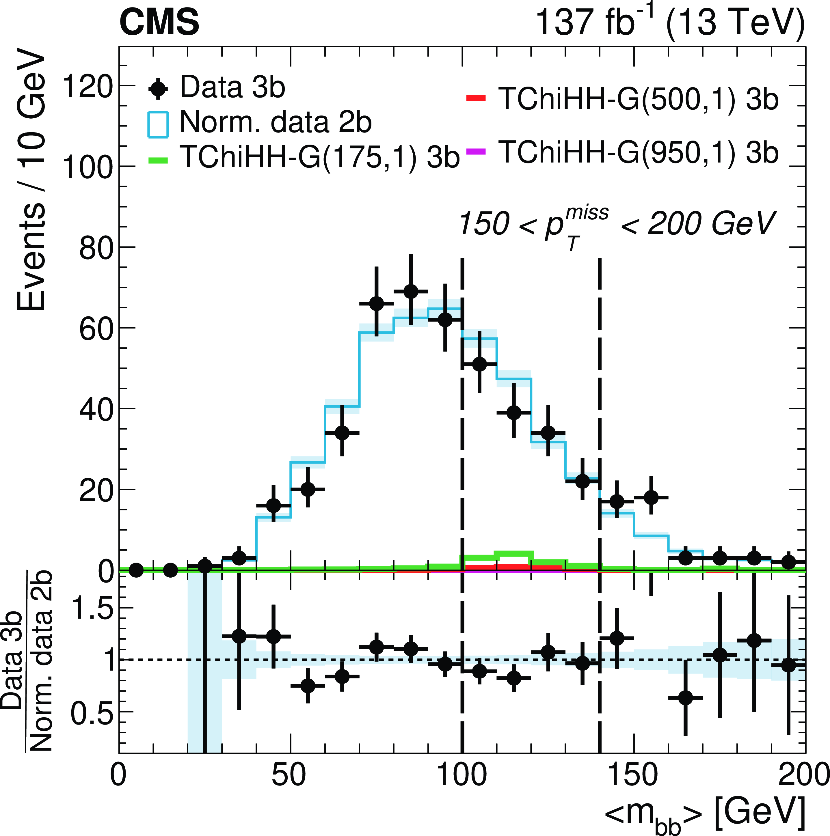
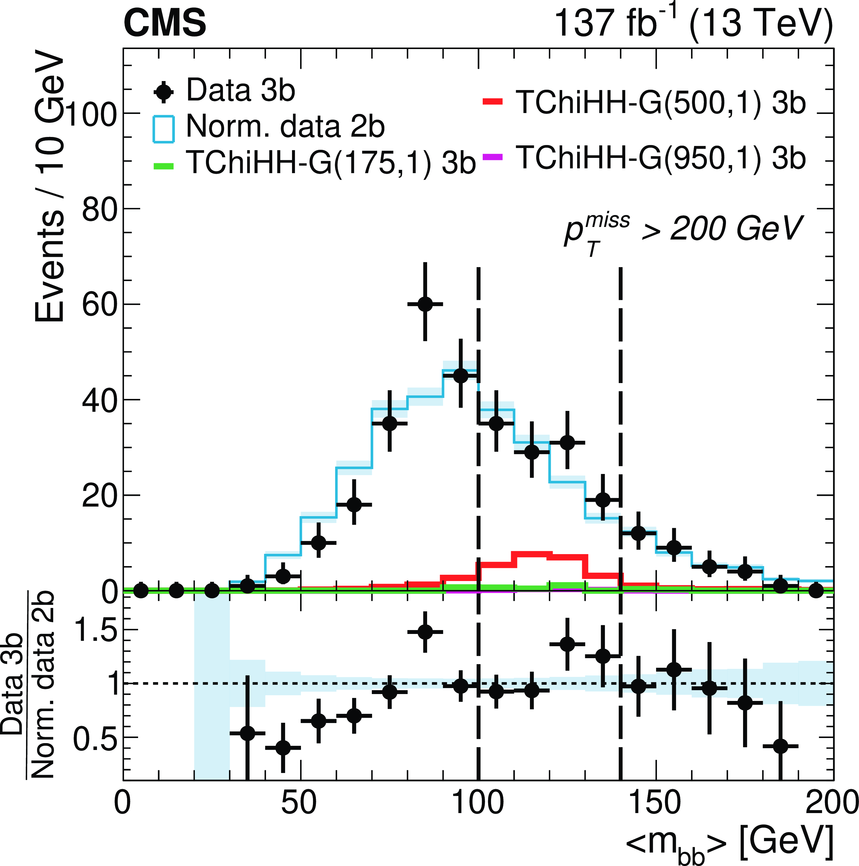
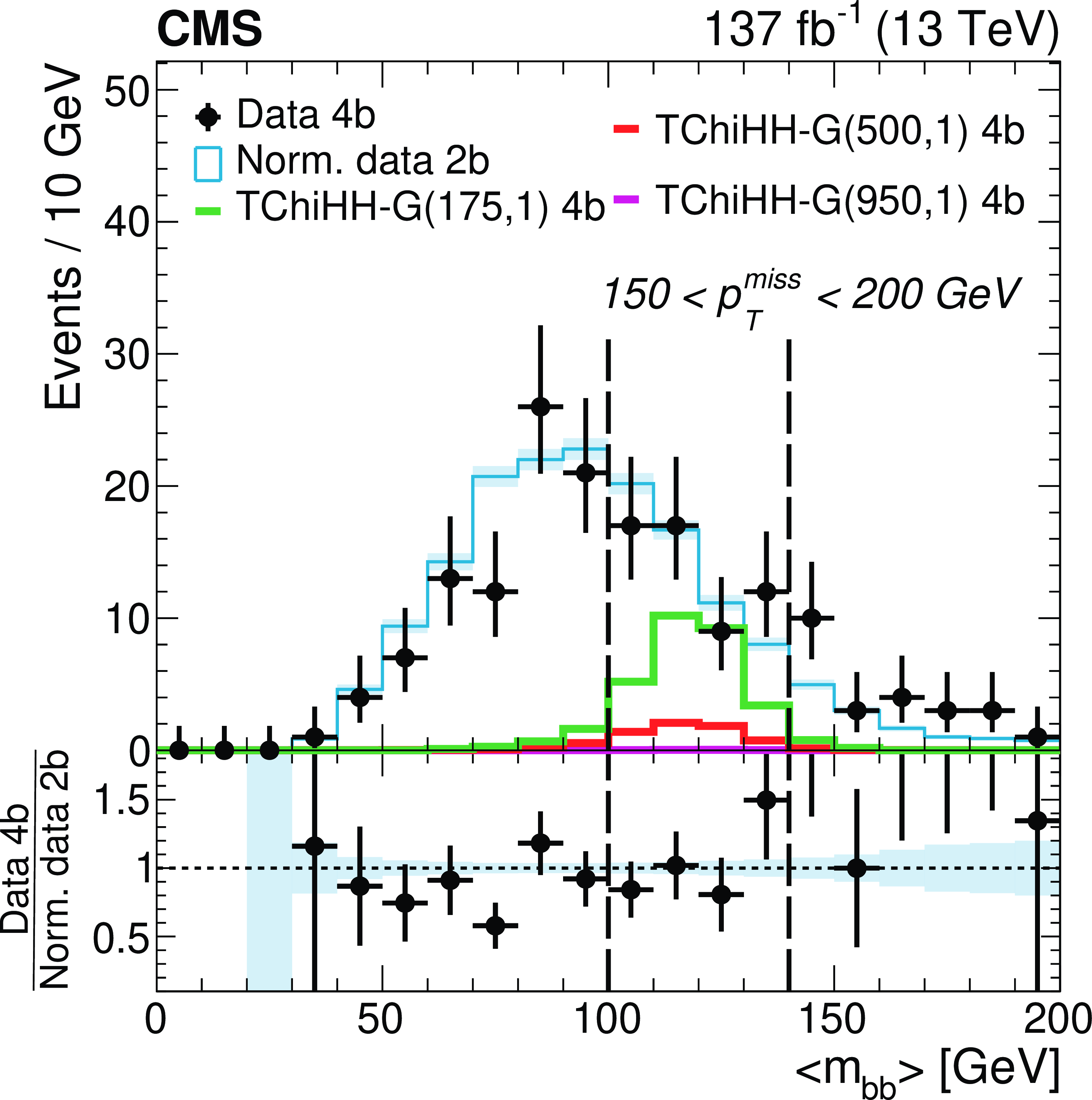
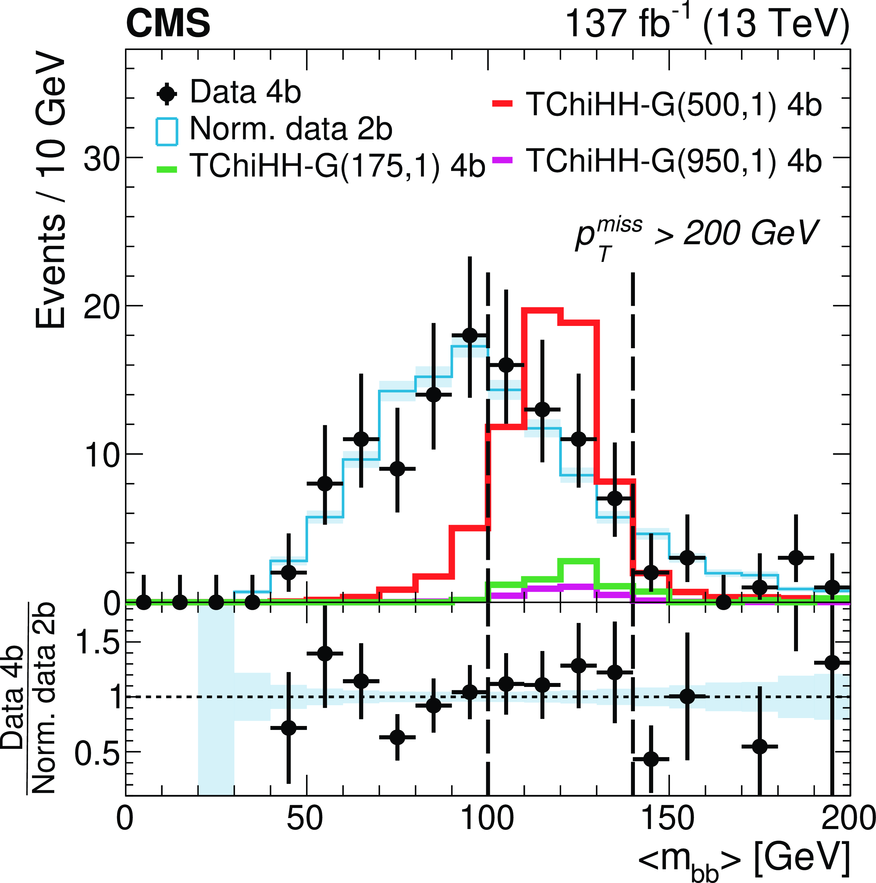
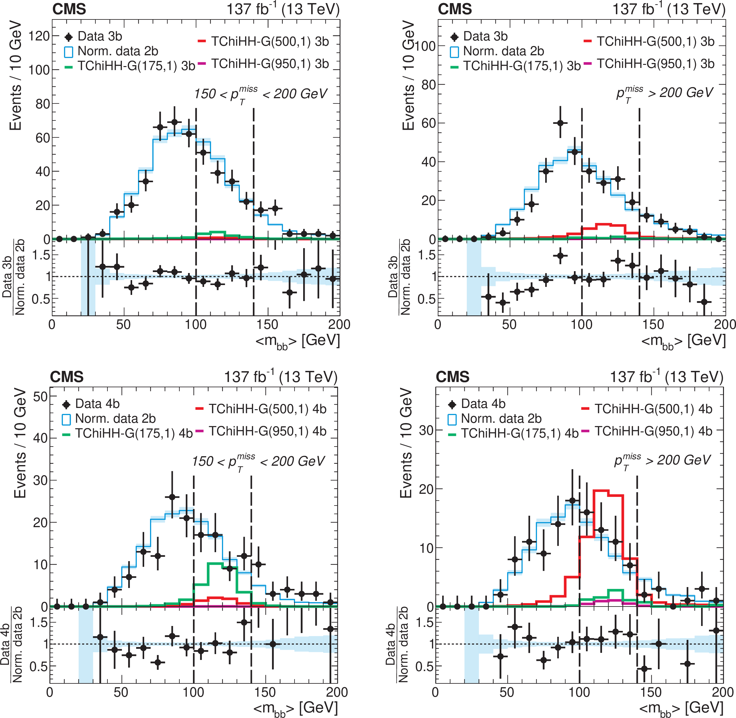
png pdf	Figure 8: Distributions in ${< m_{\mathrm{b} \mathrm{b}}>}$ for the (upper row) $ {N_\mathrm{b}} =$ 3 and (lower row) $ {N_\mathrm{b}} =$ 4 data, denoted by black markers, with error bars indicating the statistical uncertainties. The left-hand set of plots corresponds to 150 $ < {{p_{\mathrm {T}}} ^\text {miss}} < $ 200, while the right-hand set corresponds to $ {{p_{\mathrm {T}}} ^\text {miss}} > $ 200 GeV, in both cases integrated over ${\Delta R_{\text {max}}}$. The overlaid cyan histograms show the corresponding distributions of the $ {N_\mathrm{b}} =$ 2 data, reweighted with the appropriate ${\kappa}$ values and scaled in area to the $ {N_\mathrm{b}} =$ 3 or $ {N_\mathrm{b}} =$ 4 distribution and with statistical uncertainties indicated by the cyan shading. The ratio of these distributions appears in the lower panel. The red, green, and violet histograms show simulations of representative signals, denoted TChiHH-G($m(\tilde{\chi}^0_1),m(\tilde{\mathrm{G}}$) [GeV]) in the legends.
png pdf	Figure 8-a: Distribution in ${< m_{\mathrm{b} \mathrm{b}}>}$ for the $ {N_\mathrm{b}} =$ 3 data, denoted by black markers, with error bars indicating the statistical uncertainties. The plot corresponds to 150 $ < {{p_{\mathrm {T}}} ^\text {miss}} < $ 200, integrated over ${\Delta R_{\text {max}}}$. The overlaid cyan histogram shows the corresponding distributions of the $ {N_\mathrm{b}} =$ 2 data, reweighted with the appropriate ${\kappa}$ values and scaled in area to the $ {N_\mathrm{b}} =$ 3 4 distribution and with statistical uncertainties indicated by the cyan shading. The ratio of these distributions appears in the lower panel. The red, green, and violet histograms show simulations of representative signals, denoted TChiHH-G($m(\tilde{\chi}^0_1),m(\tilde{\mathrm{G}}$) [GeV]) in the legends.
png pdf	Figure 8-b: Distribution in ${< m_{\mathrm{b} \mathrm{b}}>}$ for the $ {N_\mathrm{b}} =$ 3 data, denoted by black markers, with error bars indicating the statistical uncertainties. The plot corresponds to $ {{p_{\mathrm {T}}} ^\text {miss}} > $ 200 GeV, integrated over ${\Delta R_{\text {max}}}$. The overlaid cyan histogram shows the corresponding distributions of the $ {N_\mathrm{b}} =$ 2 data, reweighted with the appropriate ${\kappa}$ values and scaled in area to the $ {N_\mathrm{b}} =$ 3 4 distribution and with statistical uncertainties indicated by the cyan shading. The ratio of these distributions appears in the lower panel. The red, green, and violet histograms show simulations of representative signals, denoted TChiHH-G($m(\tilde{\chi}^0_1),m(\tilde{\mathrm{G}}$) [GeV]) in the legends.
png pdf	Figure 8-c: Distribution in ${< m_{\mathrm{b} \mathrm{b}}>}$ for the $ {N_\mathrm{b}} =$ 4 data, denoted by black markers, with error bars indicating the statistical uncertainties. The plot corresponds to 150 $ < {{p_{\mathrm {T}}} ^\text {miss}} < $ 200, integrated over ${\Delta R_{\text {max}}}$. The overlaid cyan histogram shows the corresponding distributions of the $ {N_\mathrm{b}} =$ 2 data, reweighted with the appropriate ${\kappa}$ values and scaled in area to the $ {N_\mathrm{b}} =$ 3 4 distribution and with statistical uncertainties indicated by the cyan shading. The ratio of these distributions appears in the lower panel. The red, green, and violet histograms show simulations of representative signals, denoted TChiHH-G($m(\tilde{\chi}^0_1),m(\tilde{\mathrm{G}}$) [GeV]) in the legends.
png pdf	Figure 8-d: Distribution in ${< m_{\mathrm{b} \mathrm{b}}>}$ for the $ {N_\mathrm{b}} =$ 4 data, denoted by black markers, with error bars indicating the statistical uncertainties. The plot corresponds to $ {{p_{\mathrm {T}}} ^\text {miss}} > $ 200 GeV, integrated over ${\Delta R_{\text {max}}}$. The overlaid cyan histogram shows the corresponding distributions of the $ {N_\mathrm{b}} =$ 2 data, reweighted with the appropriate ${\kappa}$ values and scaled in area to the $ {N_\mathrm{b}} =$ 3 4 distribution and with statistical uncertainties indicated by the cyan shading. The ratio of these distributions appears in the lower panel. The red, green, and violet histograms show simulations of representative signals, denoted TChiHH-G($m(\tilde{\chi}^0_1),m(\tilde{\mathrm{G}}$) [GeV]) in the legends.
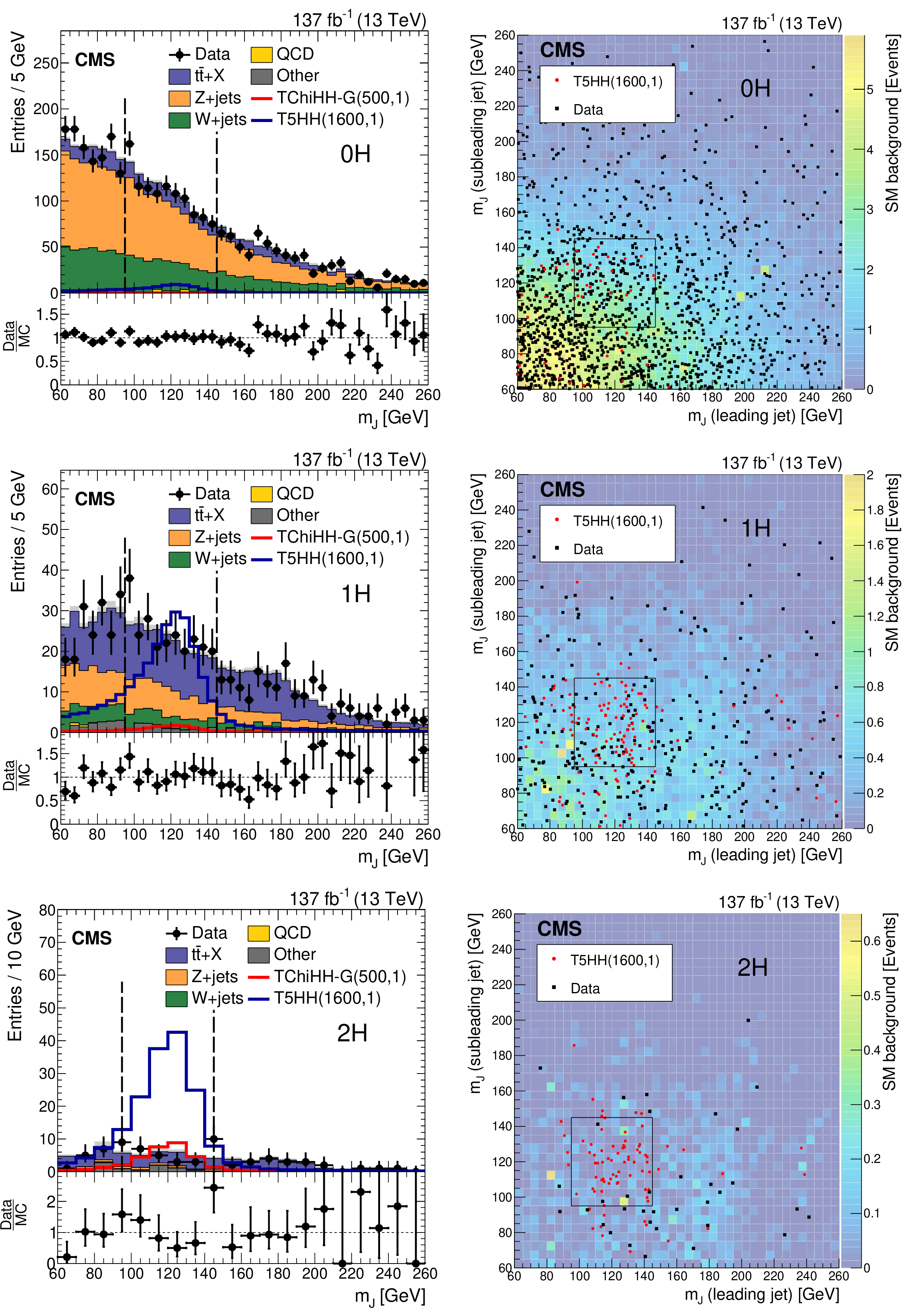
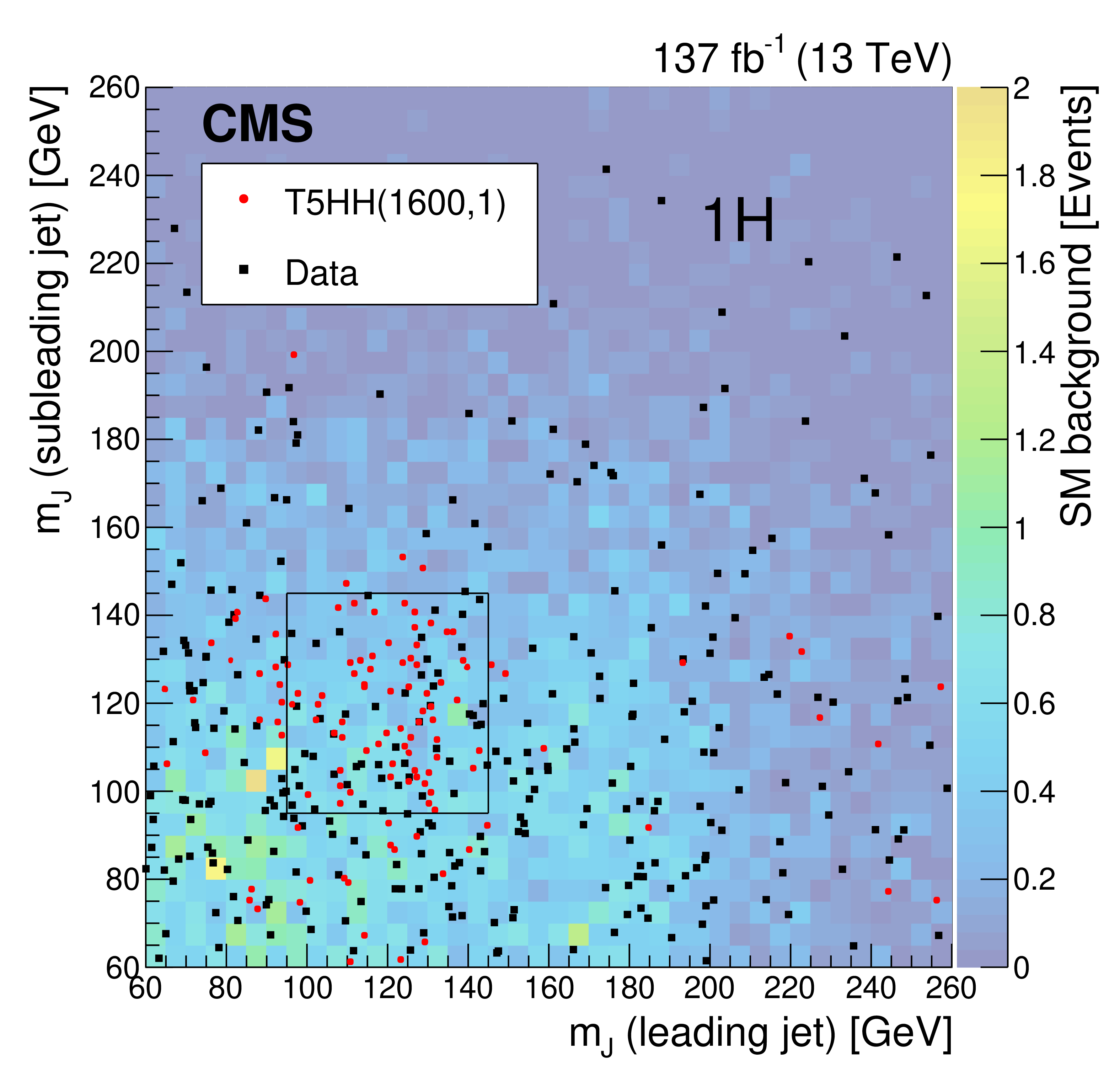
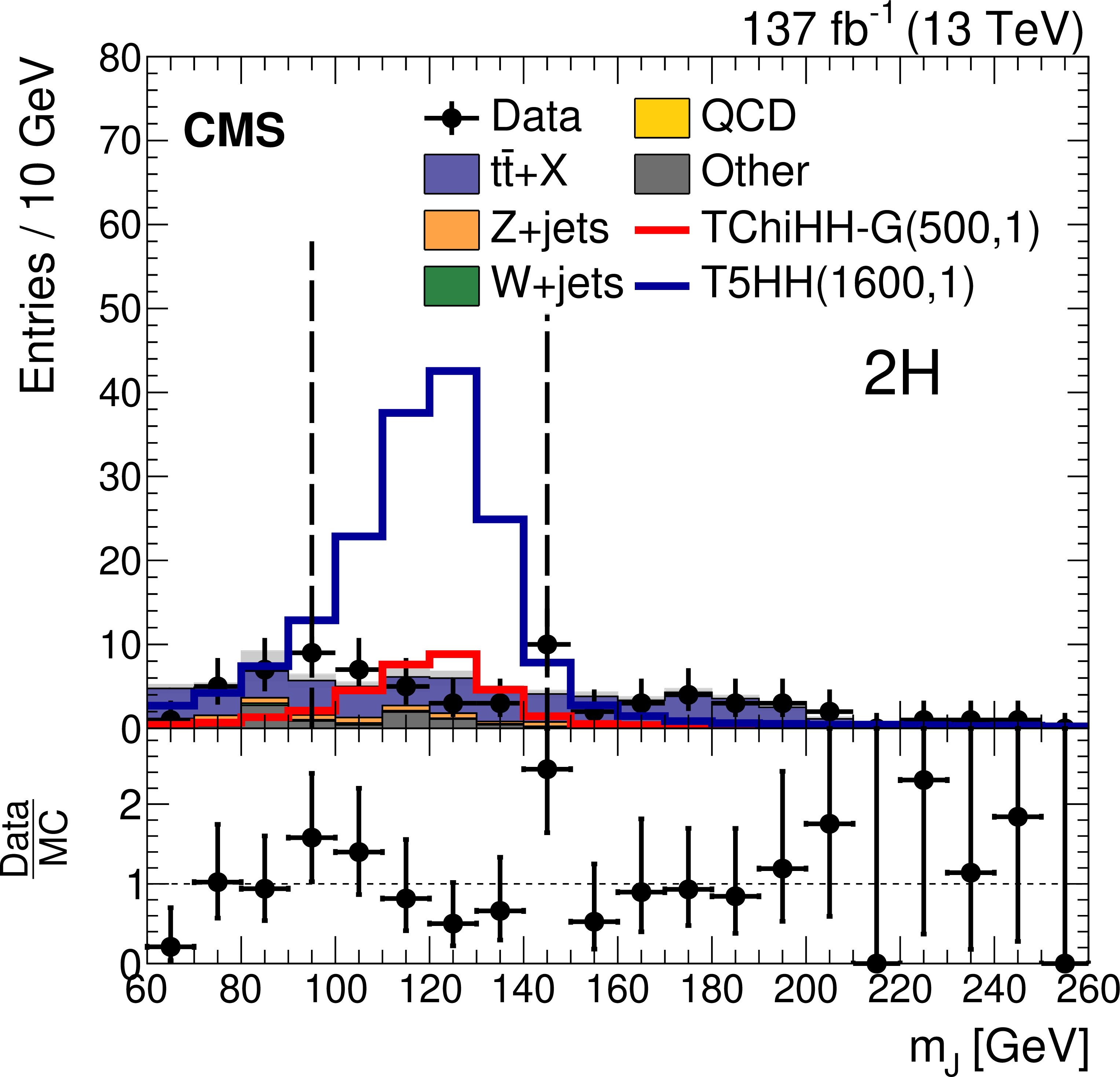
png pdf	Figure 9: Distributions in ${m_{\mathrm {J}}}$ for the boosted signature, integrated in ${{p_{\mathrm {T}}} ^\text {miss}}$. The projections (left column) contain two entries per event, with statistical uncertainties in the data and simulation given by the vertical bars and gray shading, respectively. The SM yields are scaled to the data integral, by factors of 0.84, 0.92, and 1.13 in the 0H (upper), 1H (middle), and 2H (lower) plots, respectively. The data to simulation ratio appears in each lower panel. Simulated signals TChiHH-G($m(\tilde{\chi}^0_1)$, $m(\tilde{\mathrm{G}})$) and T5HH($m({\mathrm{\widetilde{g}}})$, $m(\tilde{\chi}^0_1$)[GeV]) are also shown. In the correlation plots (right column) the color scale represents the SM background, black dots the data, and red dots the expected signal. The dashed lines and boxes denote the boundaries of the SRs.
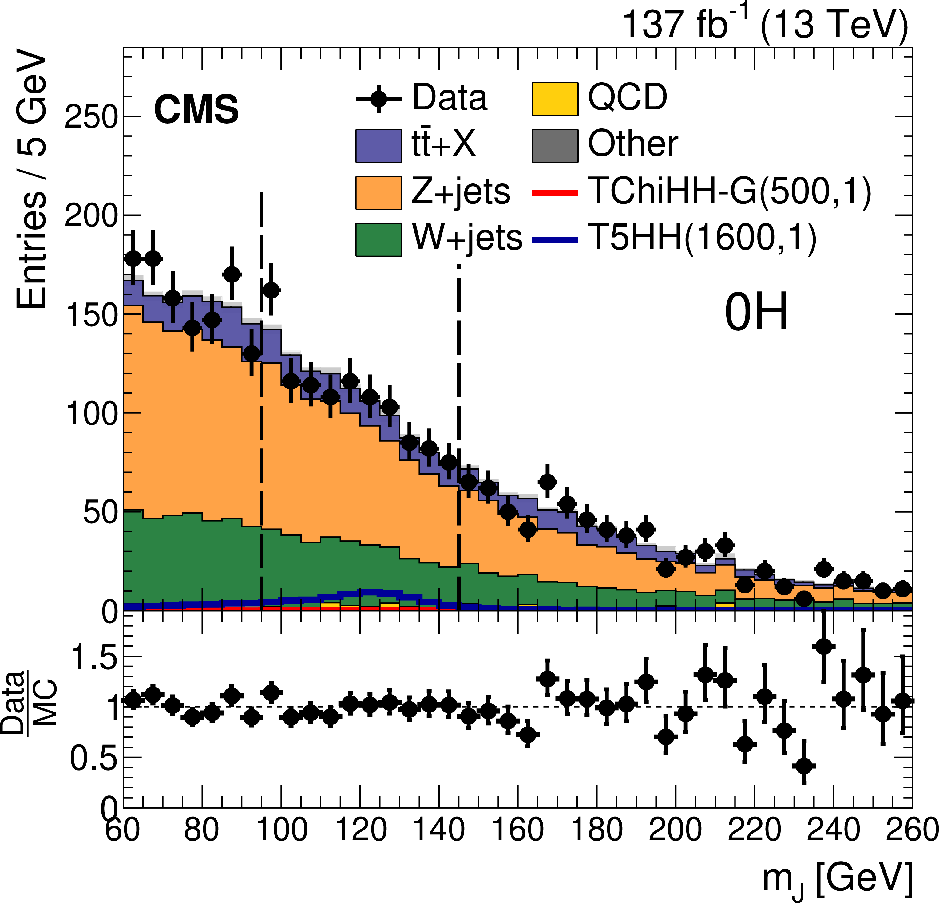
png pdf	Figure 9-a: Distribution in ${m_{\mathrm {J}}}$ for the boosted signature, integrated in ${{p_{\mathrm {T}}} ^\text {miss}}$, in the 0H region. The projection contains two entries per event, with statistical uncertainties in the data and simulation given by the vertical bars and gray shading, respectively. The SM yield is scaled to the data integral, by a factor of 0.84. The data to simulation ratio appears in the lower panel. Simulated signals TChiHH-G($m(\tilde{\chi}^0_1)$, $m(\tilde{\mathrm{G}})$) and T5HH($m({\mathrm{\widetilde{g}}})$, $m(\tilde{\chi}^0_1$)[GeV]) are also shown. The dashed lines denote the boundaries of the SR.
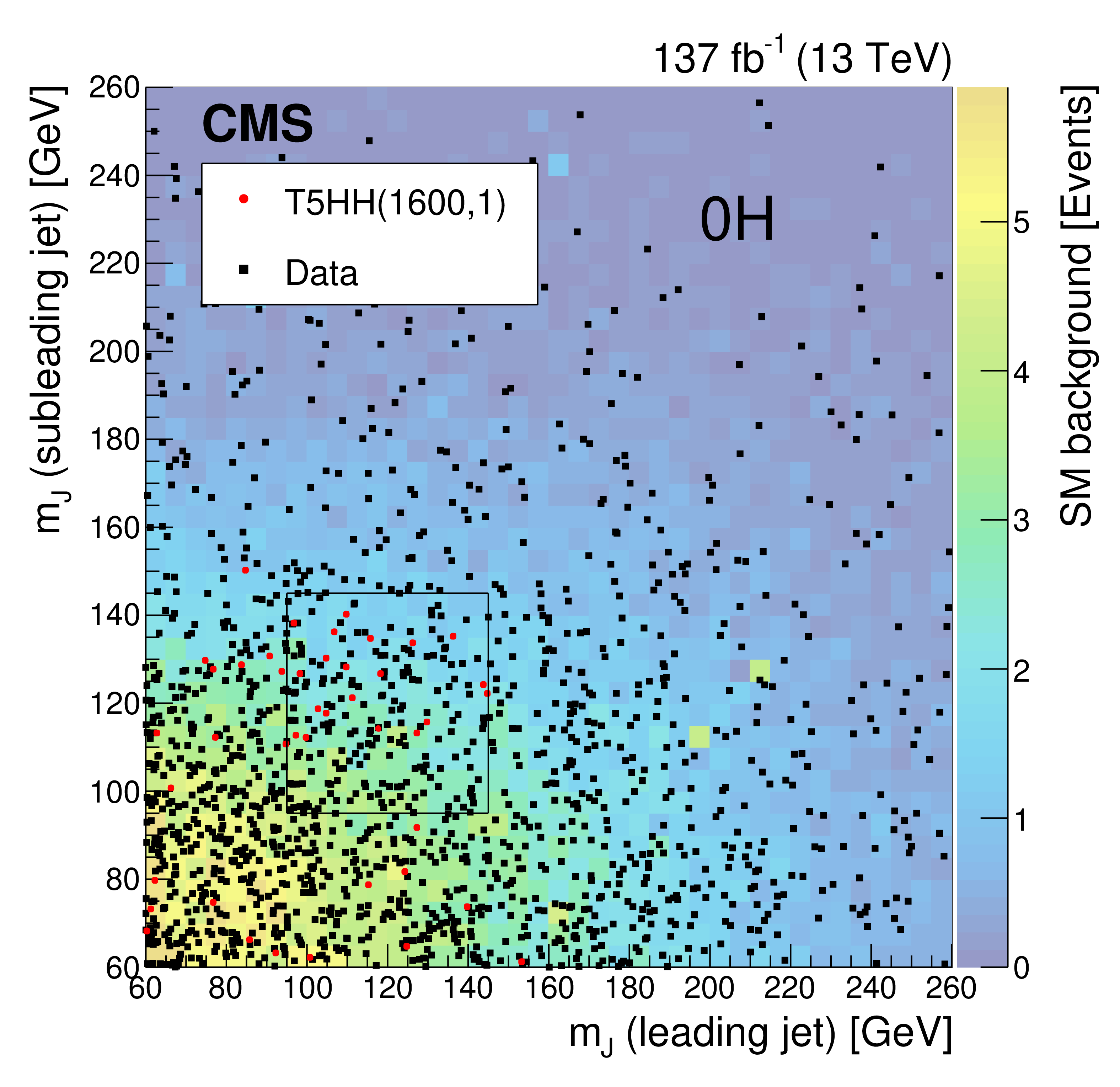
png pdf	Figure 9-b: Distribution in ${m_{\mathrm {J}}}$ for the boosted signature, integrated in ${{p_{\mathrm {T}}} ^\text {miss}}$, in the 0H region. Correlation plot, where the color scale represents the SM background, black dots the data, and red dots the expected signal. The dashed box denotes the boundary of the SR.
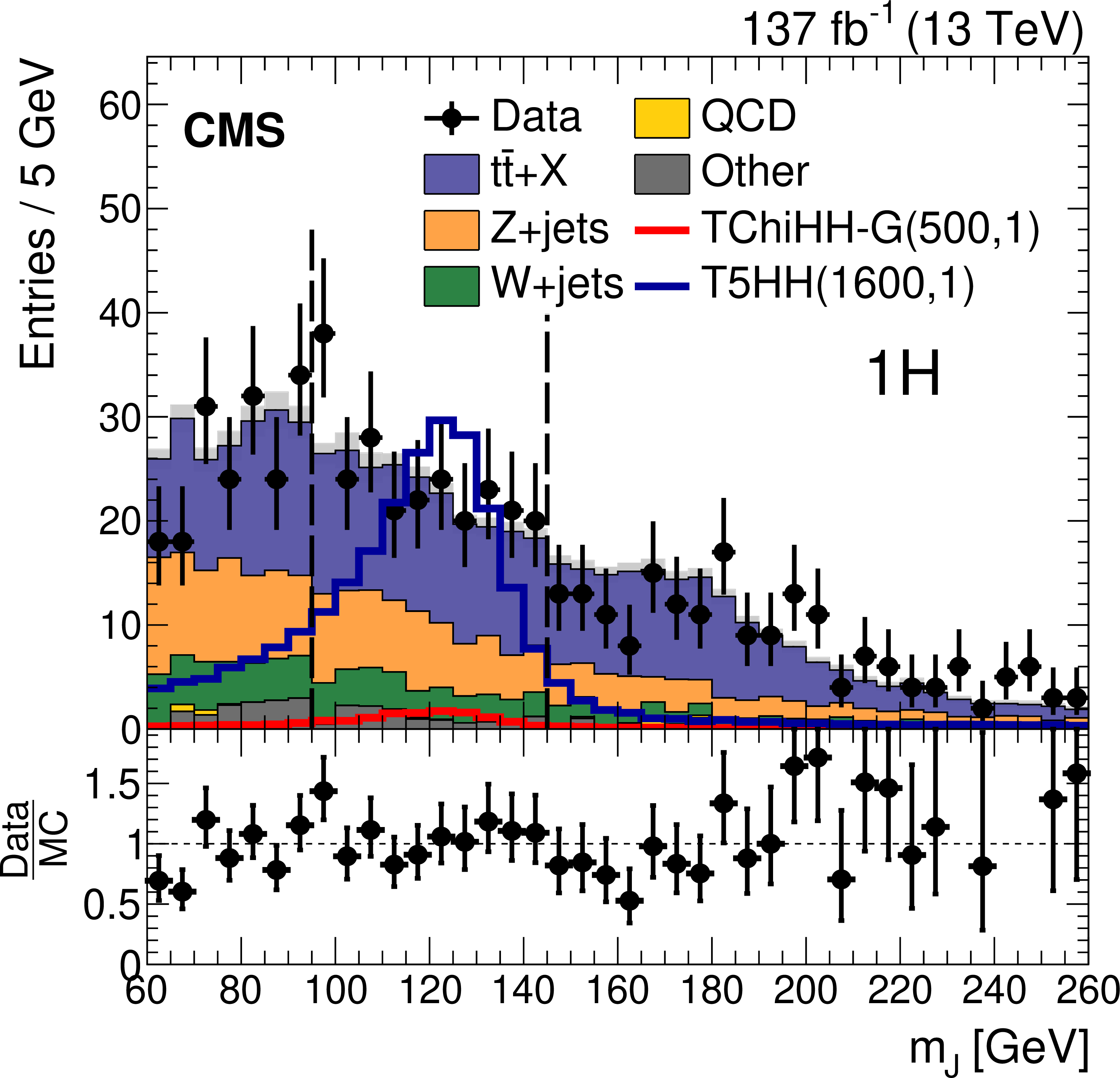
png pdf	Figure 9-c: Distribution in ${m_{\mathrm {J}}}$ for the boosted signature, integrated in ${{p_{\mathrm {T}}} ^\text {miss}}$, in the 1H region. The projection contains two entries per event, with statistical uncertainties in the data and simulation given by the vertical bars and gray shading, respectively. The SM yield is scaled to the data integral, by a factor of 0.92. The data to simulation ratio appears in the lower panel. Simulated signals TChiHH-G($m(\tilde{\chi}^0_1)$, $m(\tilde{\mathrm{G}})$) and T5HH($m({\mathrm{\widetilde{g}}})$, $m(\tilde{\chi}^0_1$)[GeV]) are also shown. The dashed lines denote the boundaries of the SR.
png pdf	Figure 9-d: Distribution in ${m_{\mathrm {J}}}$ for the boosted signature, integrated in ${{p_{\mathrm {T}}} ^\text {miss}}$, in the 1H region. Correlation plot, where the color scale represents the SM background, black dots the data, and red dots the expected signal. The dashed box denotes the boundary of the SR.
png pdf	Figure 9-e: Distribution in ${m_{\mathrm {J}}}$ for the boosted signature, integrated in ${{p_{\mathrm {T}}} ^\text {miss}}$, in the 2H region. The projection contains two entries per event, with statistical uncertainties in the data and simulation given by the vertical bars and gray shading, respectively. The SM yield is scaled to the data integral, by a factor of 1.13. The data to simulation ratio appears in the lower panel. Simulated signals TChiHH-G($m(\tilde{\chi}^0_1)$, $m(\tilde{\mathrm{G}})$) and T5HH($m({\mathrm{\widetilde{g}}})$, $m(\tilde{\chi}^0_1$)[GeV]) are also shown. The dashed lines denote the boundaries of the SR.
png pdf	Figure 9-f: Distribution in ${m_{\mathrm {J}}}$ for the boosted signature, integrated in ${{p_{\mathrm {T}}} ^\text {miss}}$, in the 2H region. Correlation plot, where the color scale represents the SM background, black dots the data, and red dots the expected signal. The dashed box denotes the boundary of the SR.
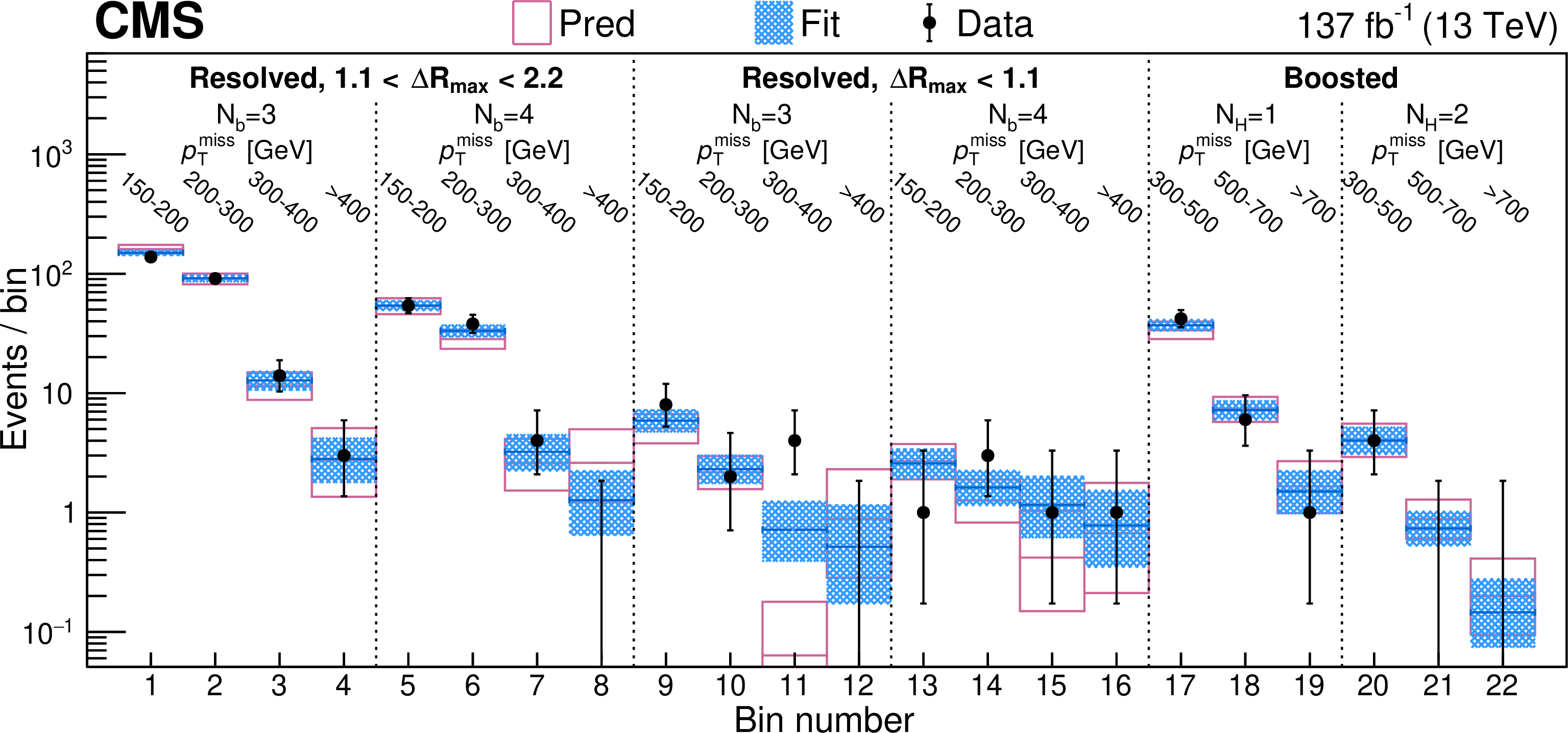
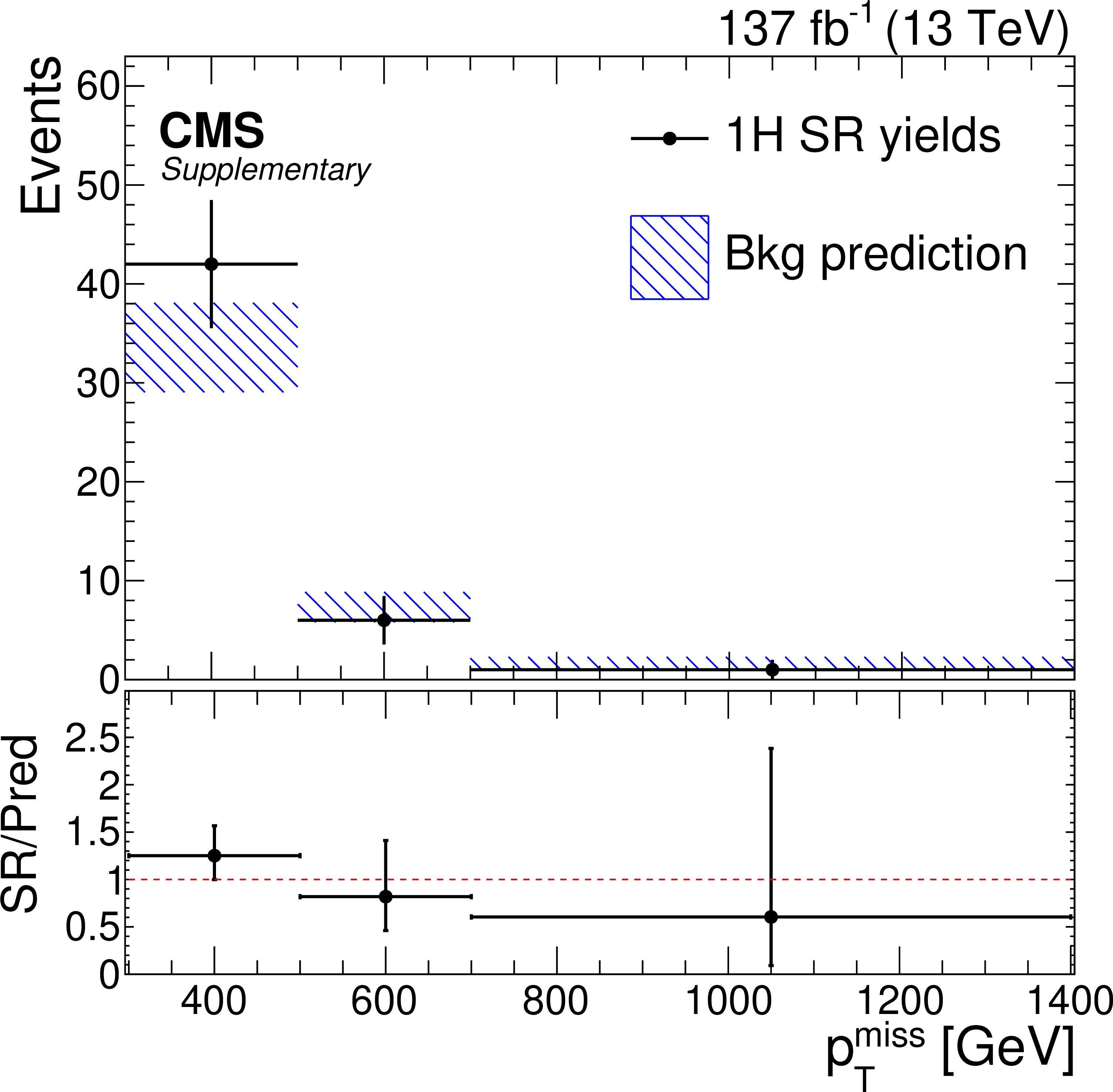
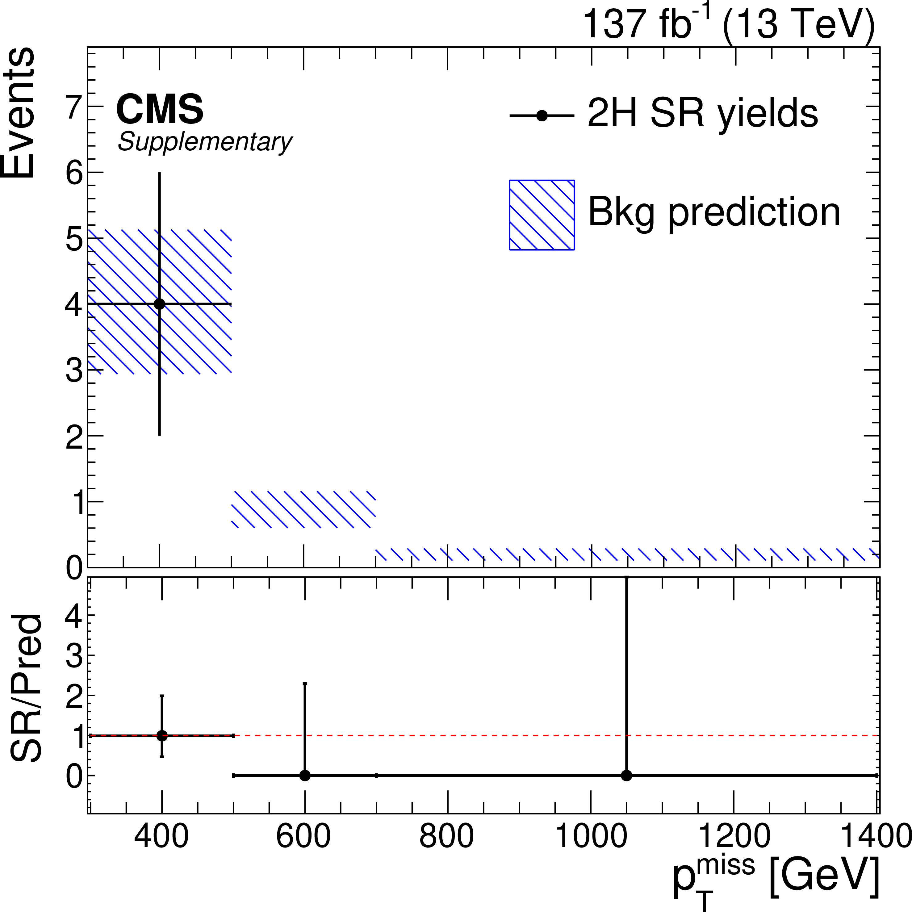
png pdf root	Figure 10: Observed and predicted yields in the search regions identified by the legend text. The points with error bars represent the observed yields, the magenta outline bands the predicted background yields ("Pred'') with their total uncertainties derived as described in Sections 7 and 8, and the blue shaded bands the values determined by the background-only fit ("Fit'').
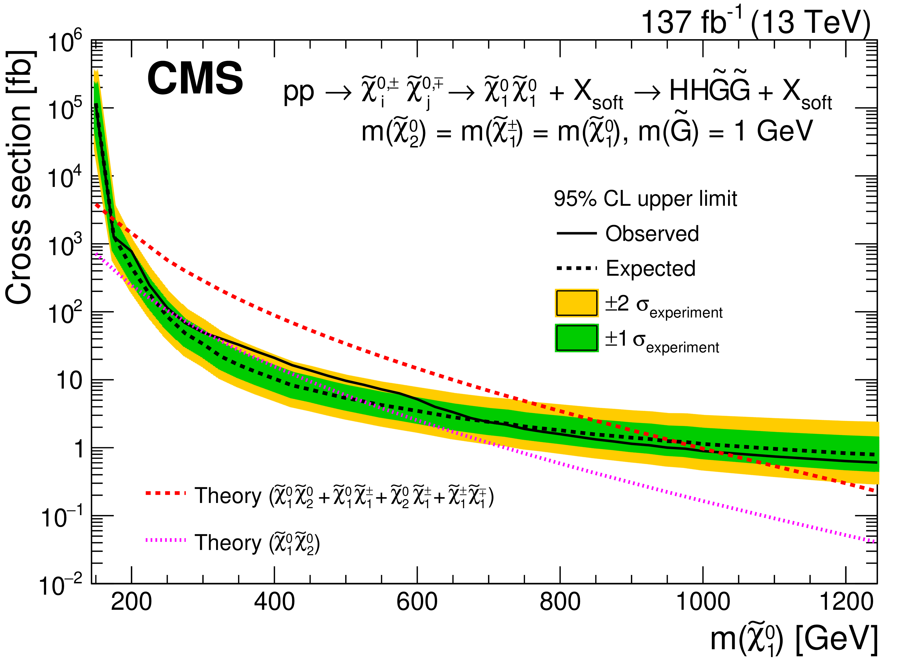
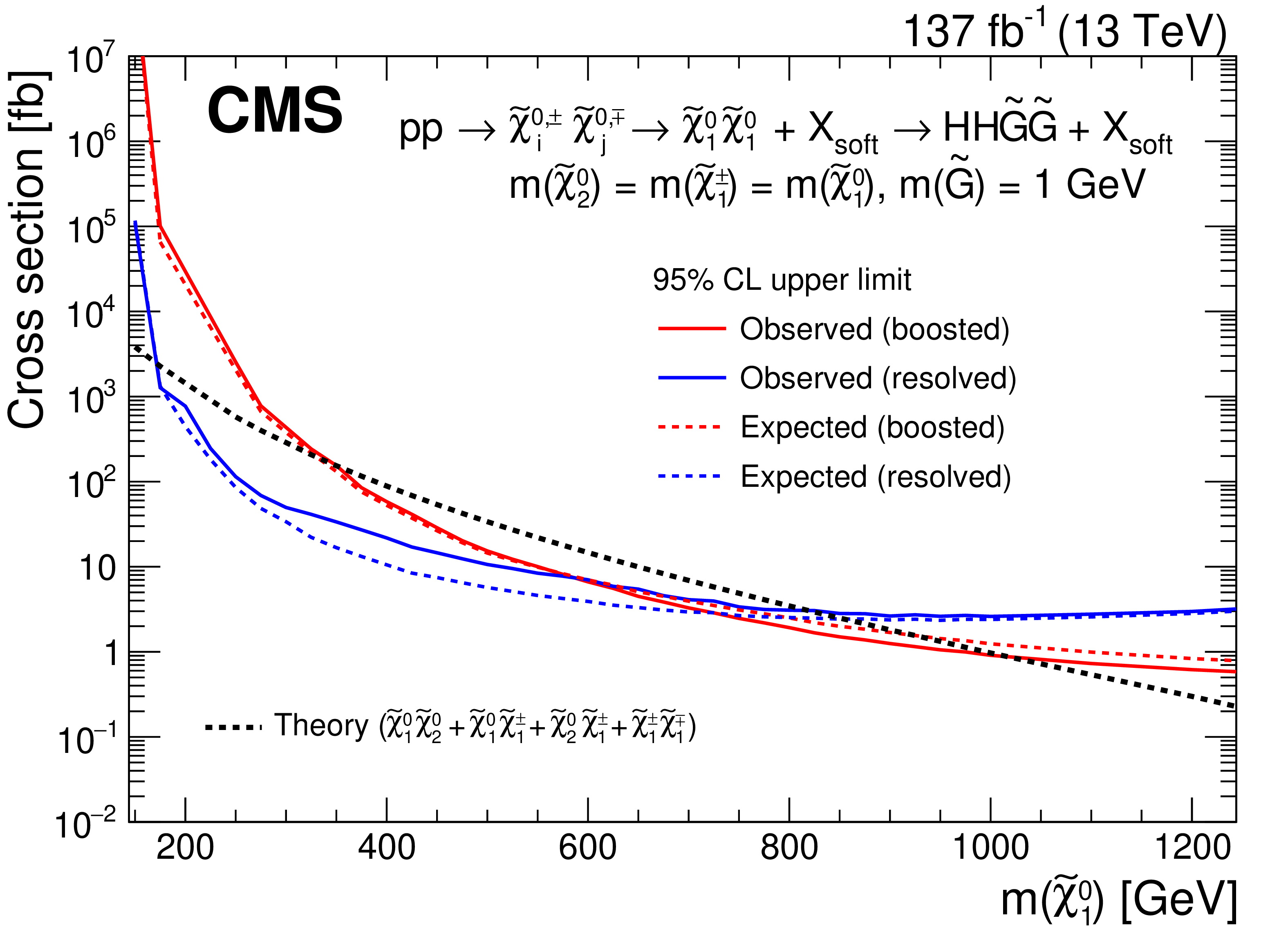
png pdf root	Figure 11: Observed and expected upper limits at 95% CL on the cross section for the GMSB-motivated simplified model TChiHH-G. The symbol $\text {X}_{\text {soft}}$ in the legend represents low-energy particles emitted in the transitions to the $\tilde{\chi}^0_1$ NLSPs. The dashed black line with green and yellow bands shows the expected limit with its 1- and 2-s.d. uncertainties, while the solid black line shows the observed limit. The theoretical cross section is indicated by the dashed red line under the assumption that the decay chains leading to the $\tilde{\chi}^0_1 \tilde{\chi}^0_1 $ intermediate state include a degenerate set of all charginos and neutralinos, and by the dotted magenta line under the assumption that only the combination $\tilde{\chi}^0_1 \tilde{\chi}^0_2 $ contributes.
png pdf	Figure 12: Separate resolved-signature (blue) and boosted-signature (red) contributions to the cross section limits for the GMSB-motivated simplified model TChiHH-G shown in Fig. 11. Here no overlapping events were removed. The symbol $\text {X}_{\text {soft}}$ in the legend represents low-energy particles emitted in the transitions to the $\tilde{\chi}^0_1$ NLSPs. The solid and dashed lines, respectively, give the observed and expected upper limits at 95% CL. The dashed black line shows the theoretical cross section computed under the assumption that the decay chains leading to the $\tilde{\chi}^0_1 \tilde{\chi}^0_1 $ intermediate state include a degenerate set of all charginos and neutralinos.
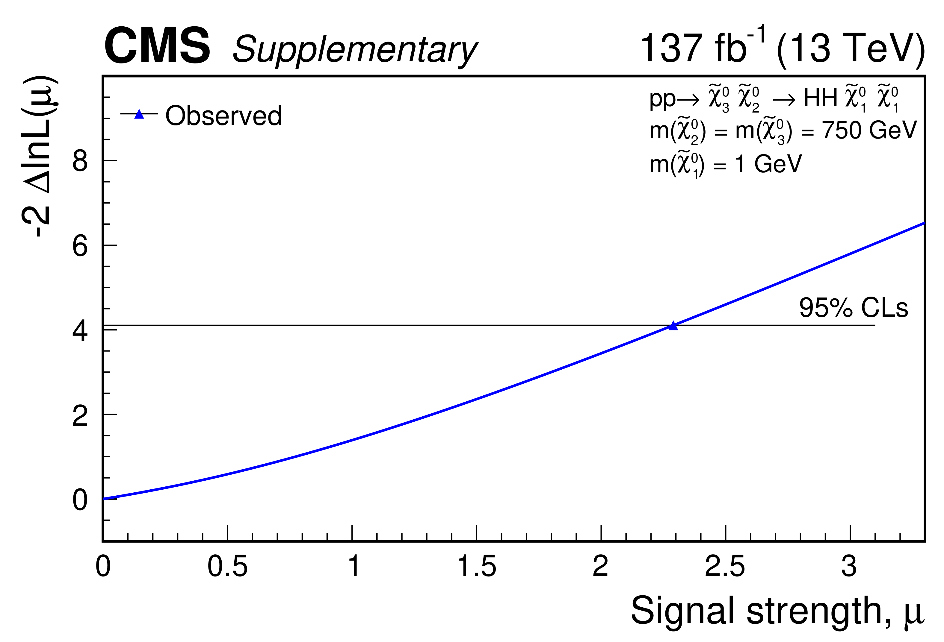
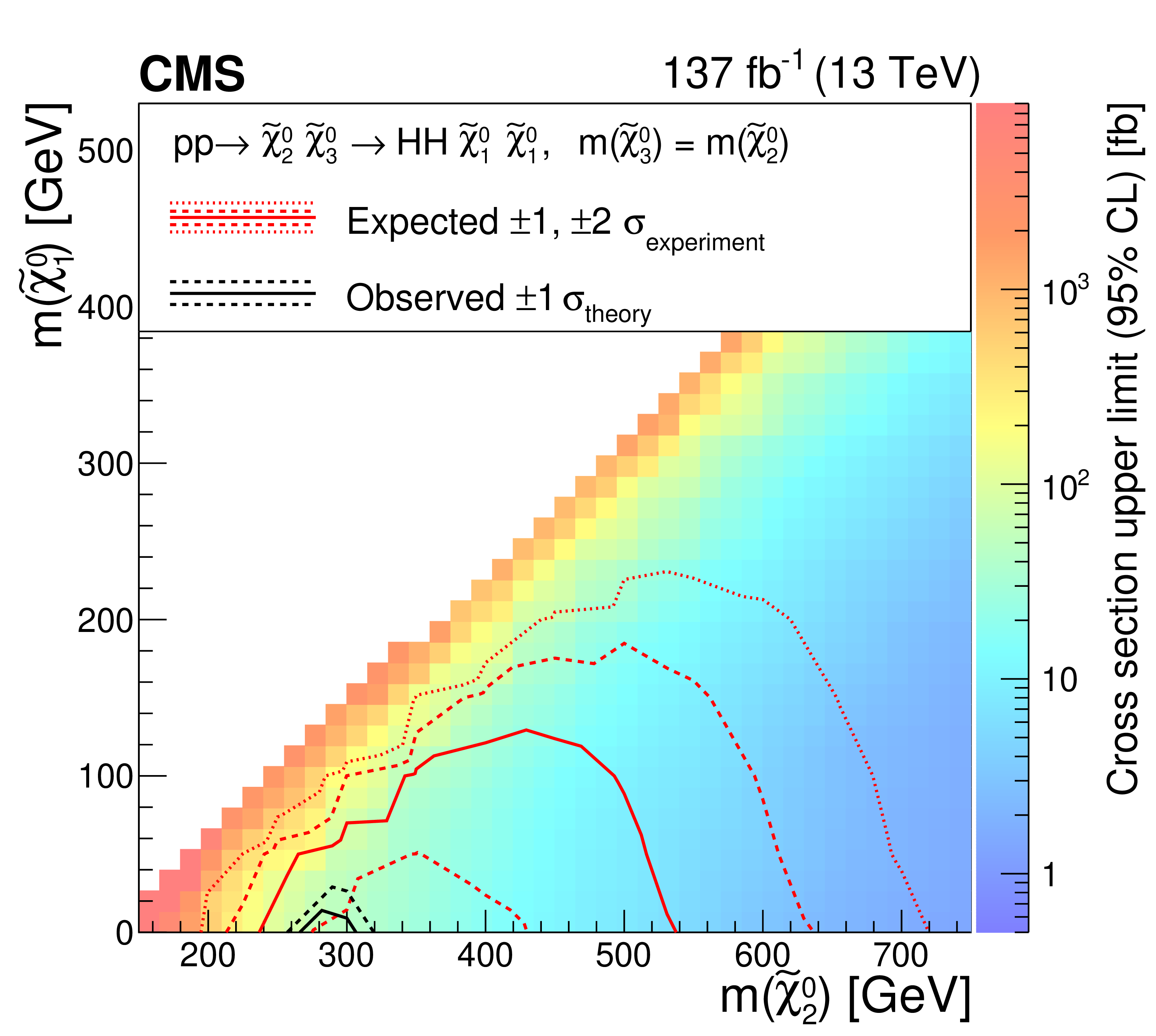
png pdf root	Figure 13: Limits at 95% CL on the cross section for the TChiHH signal model in which production of the intermediate state $\tilde{\chi}^0_2 \tilde{\chi}^0_3 $ (assumed mass degenerate) is followed by the decay of each to $\tilde{\chi}^0_1 \mathrm{H} $. The color scale gives the cross section limit as a function of $(m(\tilde{\chi}^0_2),m(\tilde{\chi}^0_1))$. The black solid and dashed curves show the observed excluded region and its 1-s.d. uncertainty. The red solid and dashed (dotted) contours show the expected excluded region with its 1 (2)-s.d. uncertainty.
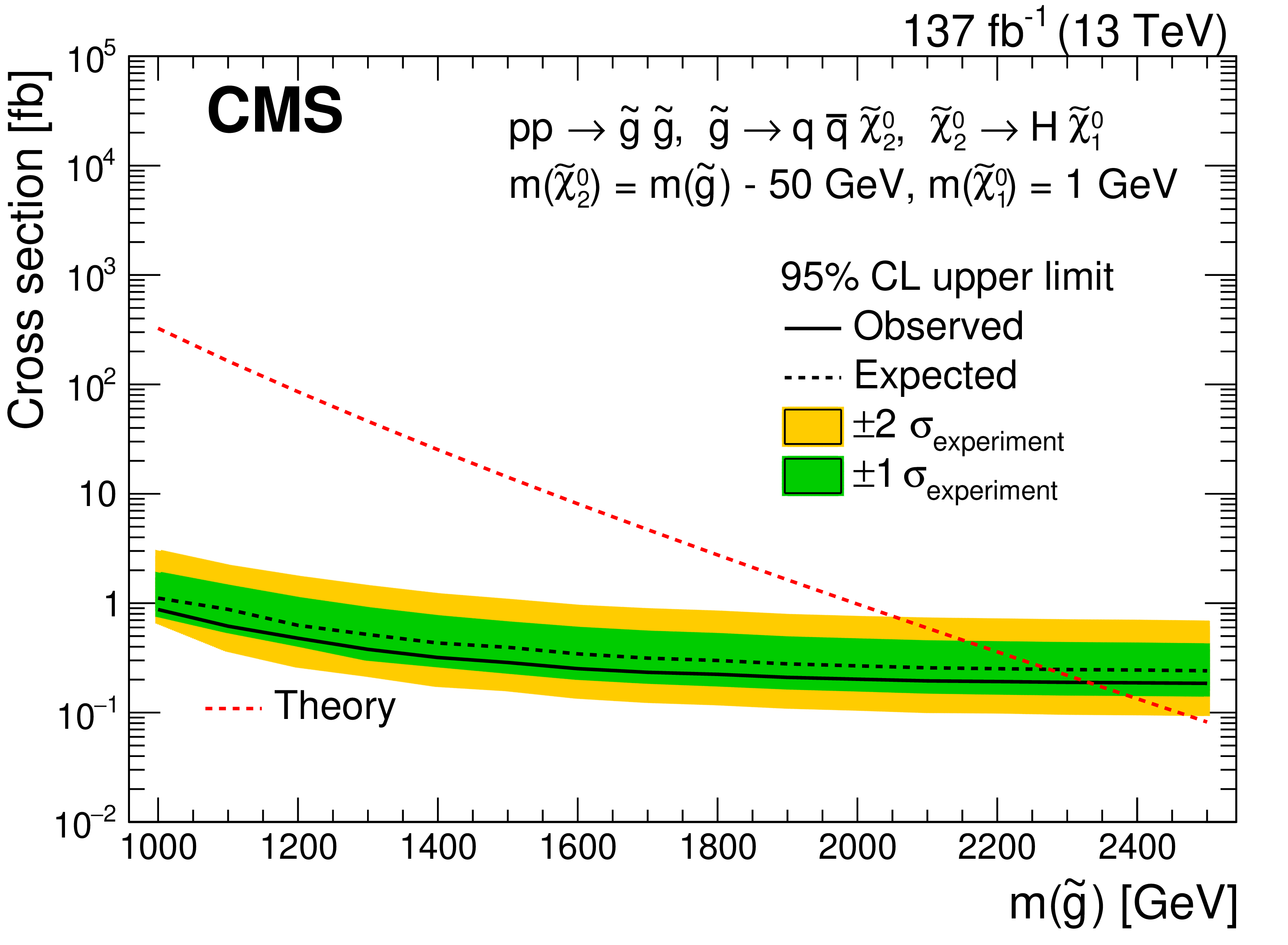
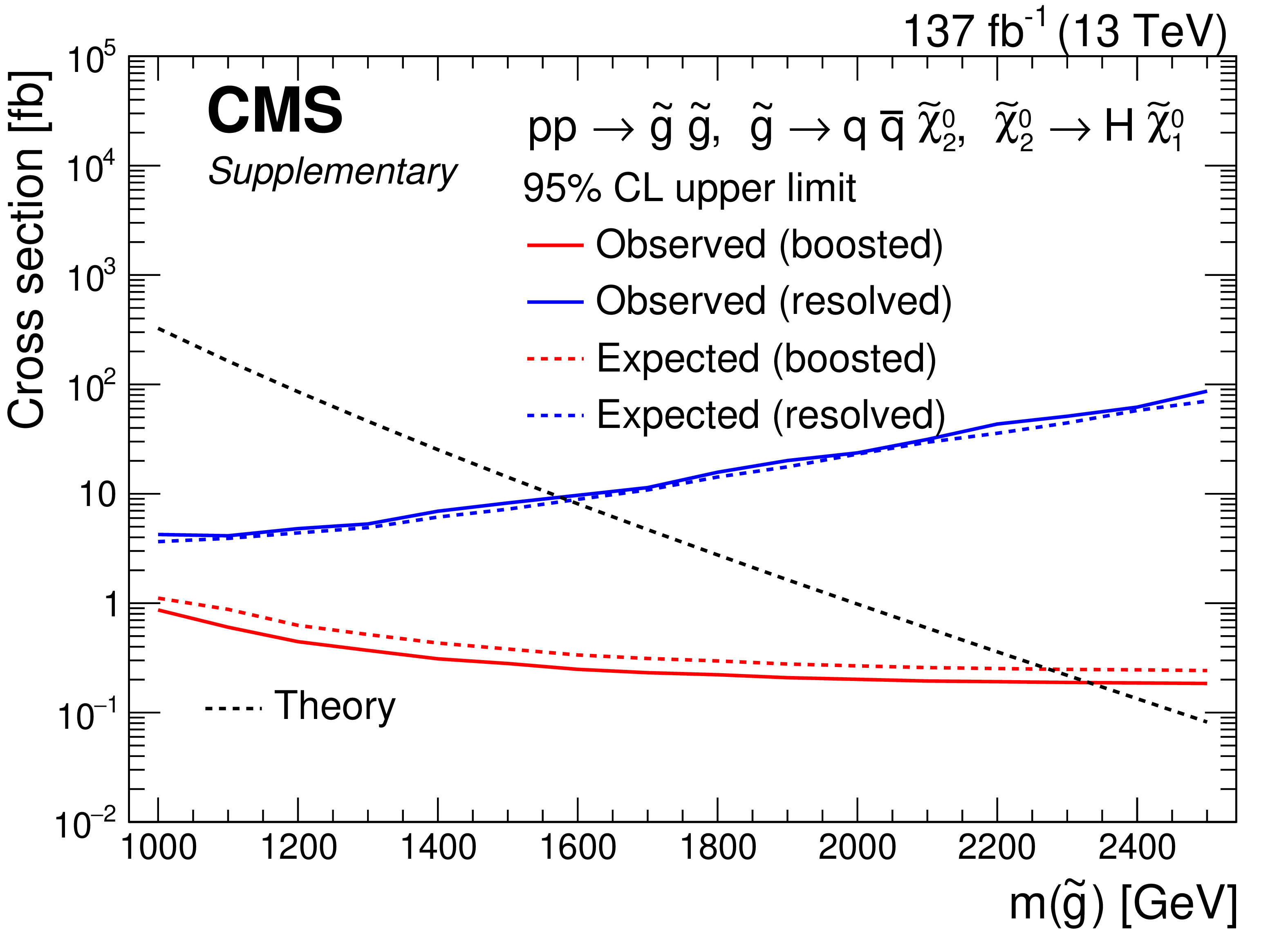
png pdf root	Figure 14: Observed and expected upper limits at 95% CL on the cross section for the simplified model T5HH, the strong production of a pair of gluinos each of which decays via a three-body process to quarks and a $\tilde{\chi}^0_2$ NLSP, which subsequently decays to a Higgs boson and a $\tilde{\chi}^0_1$ LSP. The dashed black line with green and yellow bands shows the expected limit with its 1- and 2-s.d. uncertainties; the solid black line shows the observed limit, and the dashed red line the theoretical cross section.

Tables
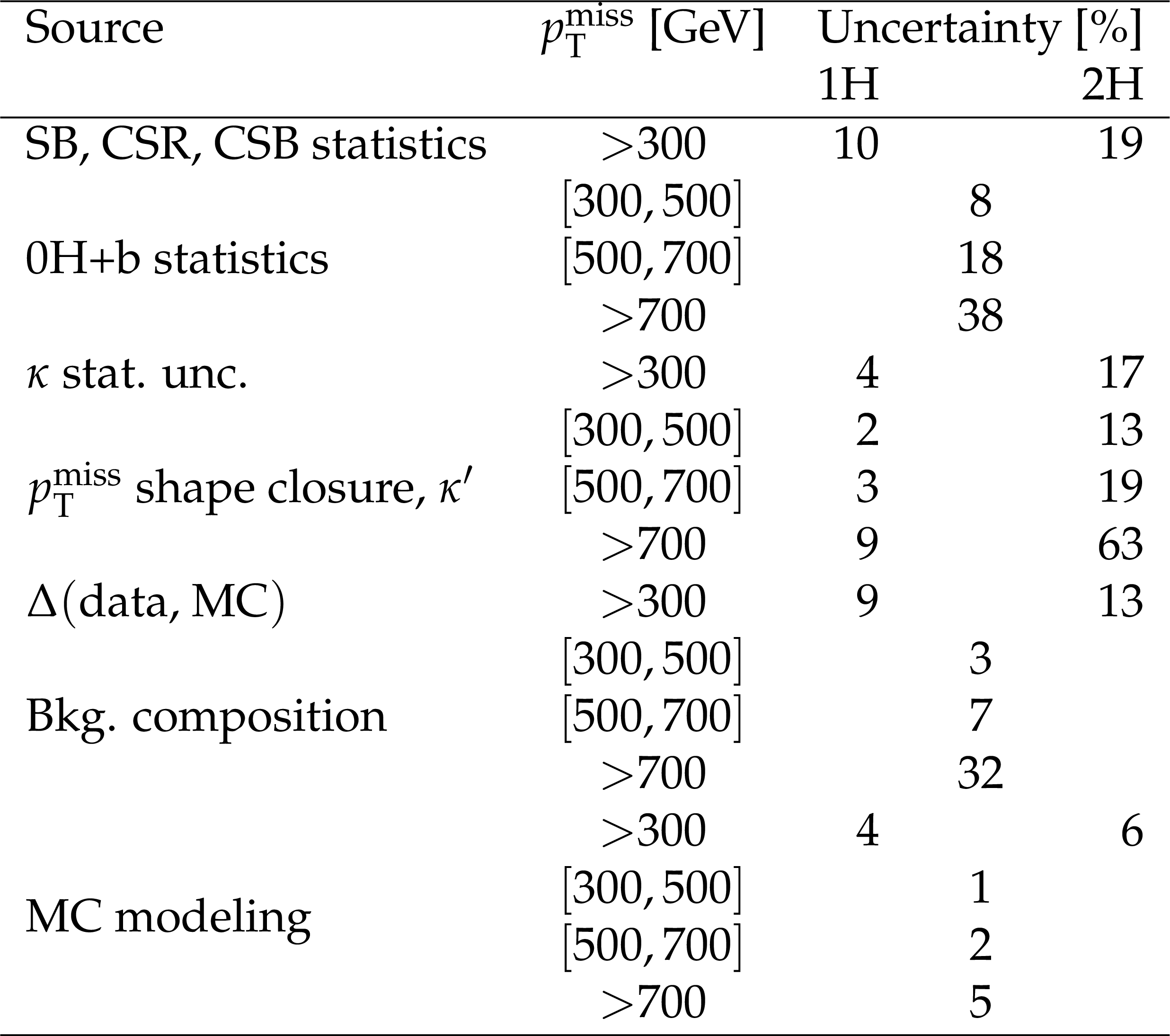
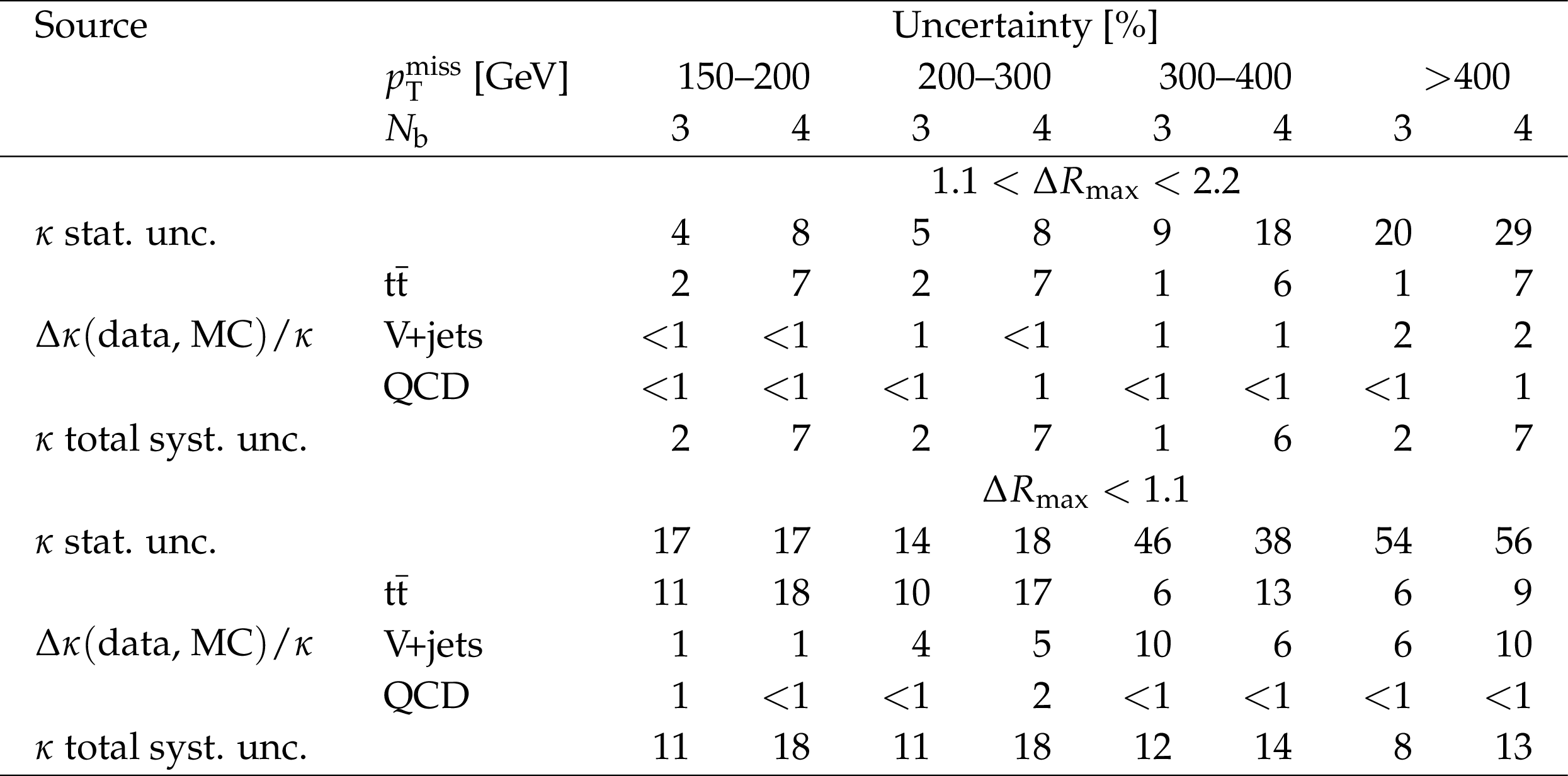
png pdf	Table 1: Summary of the uncertainties in ${\kappa}$ for the resolved signature. The sources are statistical uncertainties in the determination of ${\kappa}$ and the systematic uncertainties $\Delta \kappa (\text {data, MC})/\kappa $ derived from the comparison of simulation with data in the single-lepton, dilepton, and low-${\Delta \phi}$ control samples, each weighted by the fraction of background arising from the associated process in each search bin.
png pdf	Table 2: Summary of systematic uncertainties in the background prediction for the boosted signature. Values in cells spanning the 1H and 2H columns affect only ${f_{\text {pTmiss}}}$. The values from the ABCD measurement with the ${p_{\mathrm {T}}}$-integrated sample appear in the rows labeled $ {{p_{\mathrm {T}}} ^\text {miss}} > $ 300 GeV. The row labeled $\Delta (\text {data, MC})$ gives the contribution derived from the comparison of simulation with data in the one-lepton control sample.
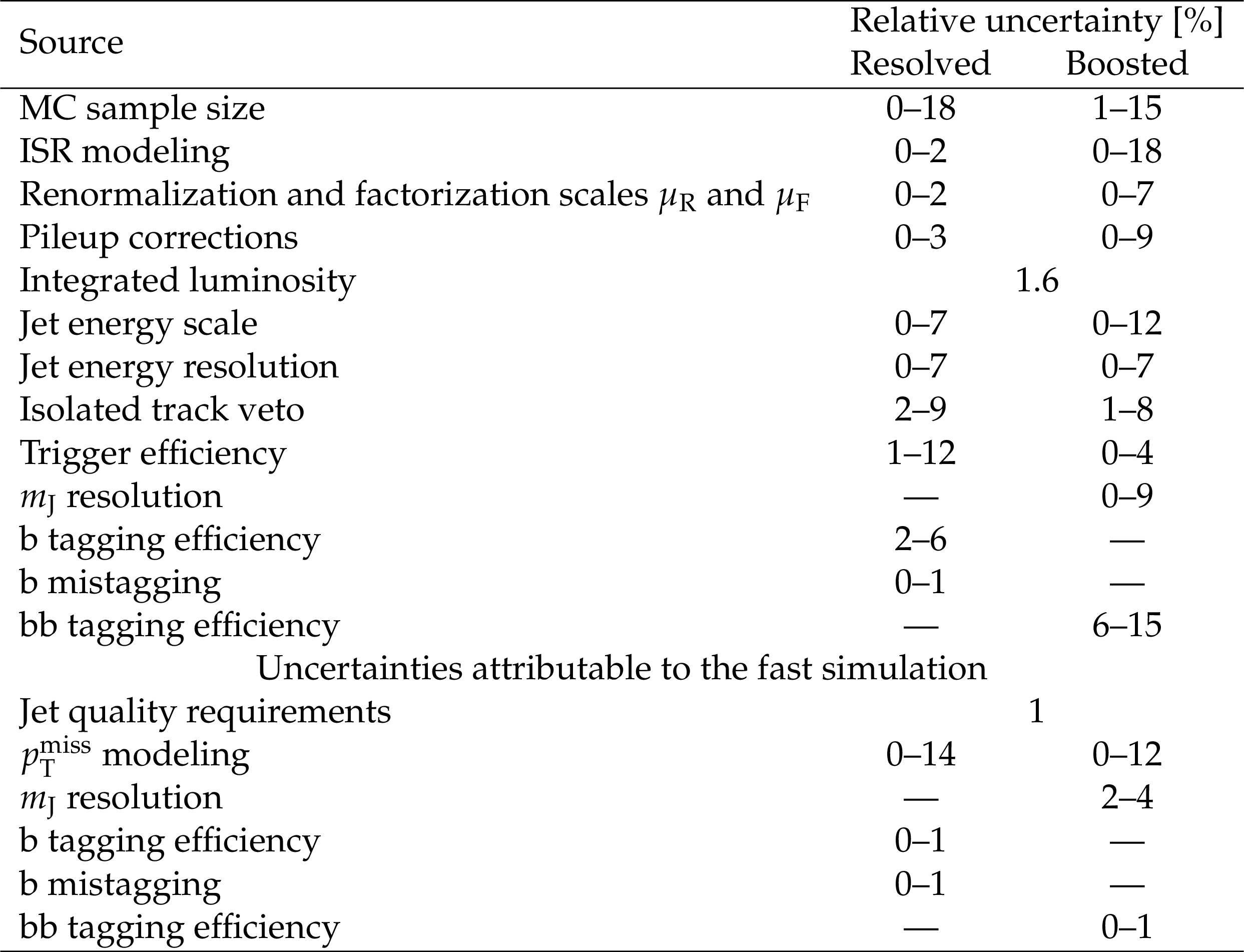
png pdf	Table 3: Sources of systematic uncertainties and their typical impact on the signal yields obtained from simulation. The range is reported as the median 68% confidence interval among all signal regions for every signal mass point considered. Entries reported as 0 correspond to values smaller than 0.5%.
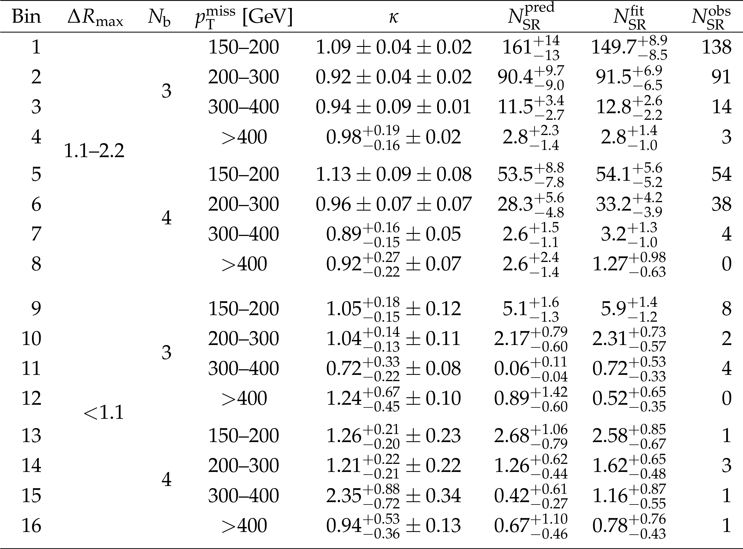
png pdf	Table 4: For each SR of the resolved signature, the MC correction factor ${\kappa}$, predicted background yield ${N_{\text {SR}}^{\text {pred}}}$, yield from the background-only ($\mu =$ 0) fit ${N_{\text {SR}}^{\text {fit}}}$, and observed yield ${N_{\text {SR}}^{\text {obs}}}$. The first and second uncertainties in the ${\kappa}$ factors are statistical and systematic, respectively. The uncertainties in ${N_{\text {SR}}^{\text {pred}}}$ and ${N_{\text {SR}}^{\text {fit}}}$, extracted from the maximum likelihood fit, include both statistical and systematic contributions. The interpretation of the results in bin 11 is discussed in the text.
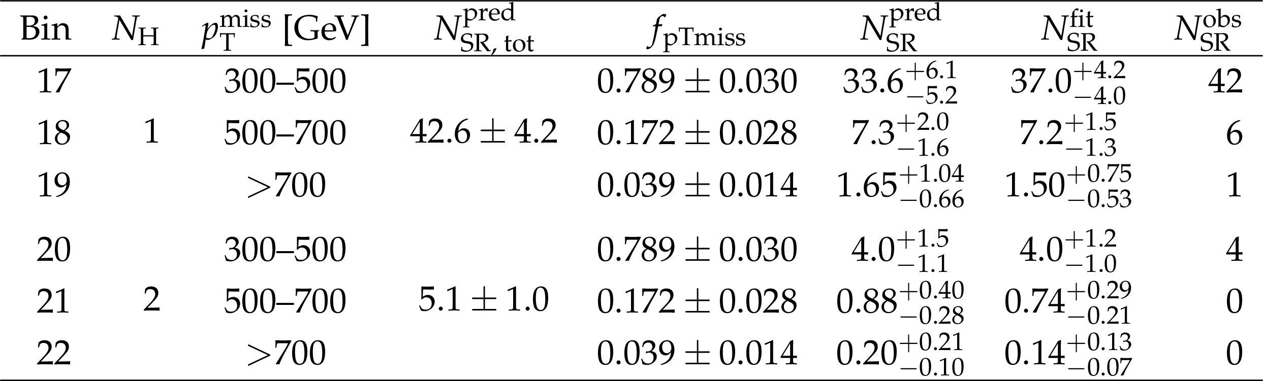
png pdf	Table 5: For each ${N_{\mathrm {\mathrm{H}}}}$ SR of the boosted signature, the total predicted background yield ${N_{\text {SR, tot}}^{\text {pred}}}$, and for each ${{p_{\mathrm {T}}} ^\text {miss}}$ bin the fraction ${f_{\text {pTmiss}}}$, both with their statistical uncertainties, the predicted background yield ${N_{\text {SR}}^{\text {pred}}}$, the yield from the background-only ($\mu =$ 0) fit ${N_{\text {SR}}^{\text {fit}}}$, and the observed yield ${N_{\text {SR}}^{\text {obs}}}$. The values of ${N_{\text {SR}}^{\text {pred}}}$ and ${N_{\text {SR}}^{\text {fit}}}$ are extracted from the maximum likelihood fit, with uncertainties that include both statistical and systematic contributions.

Summary

A search has been presented for physics beyond the standard model in channels leading to pairs of Higgs bosons and an imbalance of transverse momentum, produced in proton-proton collisions at $\sqrt{s} = $ 13 TeV. The data sample, collected by the CMS experiment at the LHC, corresponds to an integrated luminosity of 137 fb$^{-1}$. The Higgs bosons are reconstructed via their decay to a pair of b quarks, observed either as distinct b quark jets (resolved signature), or as wide-angle jets that each contain the pair of b quarks (boosted signature). The observed event yields in 15 of the 16 analysis bins of the resolved signature, and all 6 bins of the boosted signature, are consistent with the background predictions based on SM processes. In one bin of the resolved signature, an excess is observed, for which the global significance is 2.1 standard deviations when all 16 bins are considered. A narrow, single-bin effect is not typical of the supersymmetry (SUSY) models under consideration. These results are used to set limits on the cross sections for the production of particles predicted by SUSY, considering both the direct production of neutralinos and their production through intermediate states with gluinos. For the electroweak production of nearly-degenerate higgsinos, each of whose decay cascades yields a ${\tilde{\chi}^0_1}$ that in turn decays through a Higgs boson to the lightest SUSY particle (LSP), a massless goldstino, $\tilde{\chi}^0_1$ masses in the range 175-1025 GeV are excluded at 95% confidence level. For a model with a mass splitting between the directly produced, degenerate higgsinos $\tilde{\chi}^0_2 \tilde{\chi}^0_3$, and a bino LSP, a small region where $m(\tilde{\chi}^0_1)$ is less than 15 GeV is excluded; for $m(\tilde{\chi}^0_1) = $ 1 GeV the excluded range of $m(\tilde{\chi}^0_2)$ is 265-305 GeV. For the strong production of gluino pairs decaying via a slightly lighter $\tilde{\chi}^0_2$ to a Higgs boson and a light $\tilde{\chi}^0_1$ LSP, gluino masses below 2330 GeV are excluded. The bounds on masses found here extend previous limits for these models by about 150 and 320 GeV for the $\tilde{\chi}^0_1$ and gluino, respectively.

Additional Figures
png pdf	Additional Figure 1: Upper limit exclusion at 95% CL for the gluino model T5HH shown for the boosted-only and resolved-only approaches, comparing expected and observed. Overlapping events were not removed.
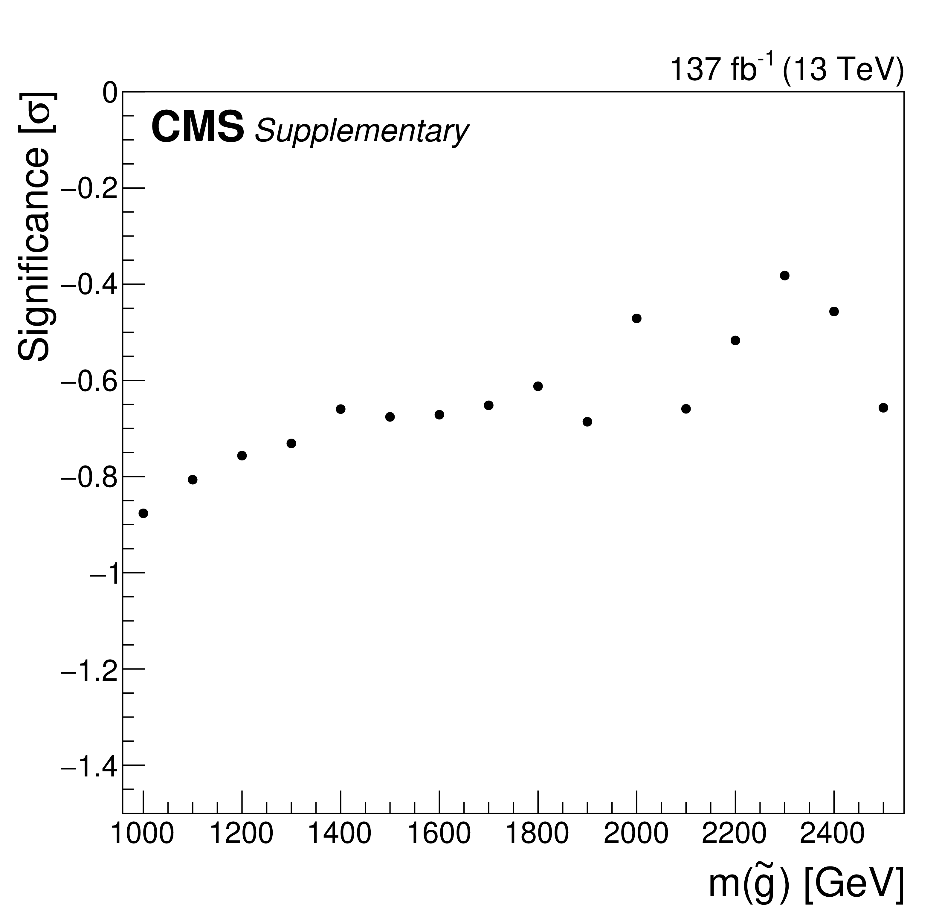
png pdf	Additional Figure 2: The significance scan for the TChiHH model (a) and the T5HH model (b) for the combination of resolved and boosted signatures. The value of the significance is signed negative where the best-fit value of the signal strength is negative (observation is less than the background estimate). The highest significance for the TChiHH model is 2.0$\sigma $ at the $ m(\tilde{\chi}_2^0)= $ 450 GeV, $ m(\tilde{\chi}^0_1)=$ 50 GeV mass point.
png pdf root	Additional Figure 2-a: The significance scan for the T5HH model for the combination of resolved and boosted signatures. The value of the significance is signed negative where the best-fit value of the signal strength is negative (observation is less than the background estimate).
png pdf root	Additional Figure 2-b: The significance scan for the TChiHH model (a) and the T5HH model (b) for the combination of resolved and boosted signatures. The value of the significance is signed negative where the best-fit value of the signal strength is negative (observation is less than the background estimate). The highest significance for the TChiHH model is 2.0$\sigma $ at the $ m(\tilde{\chi}_2^0)= $ 450 GeV, $ m(\tilde{\chi}^0_1)=$ 50 GeV mass point.
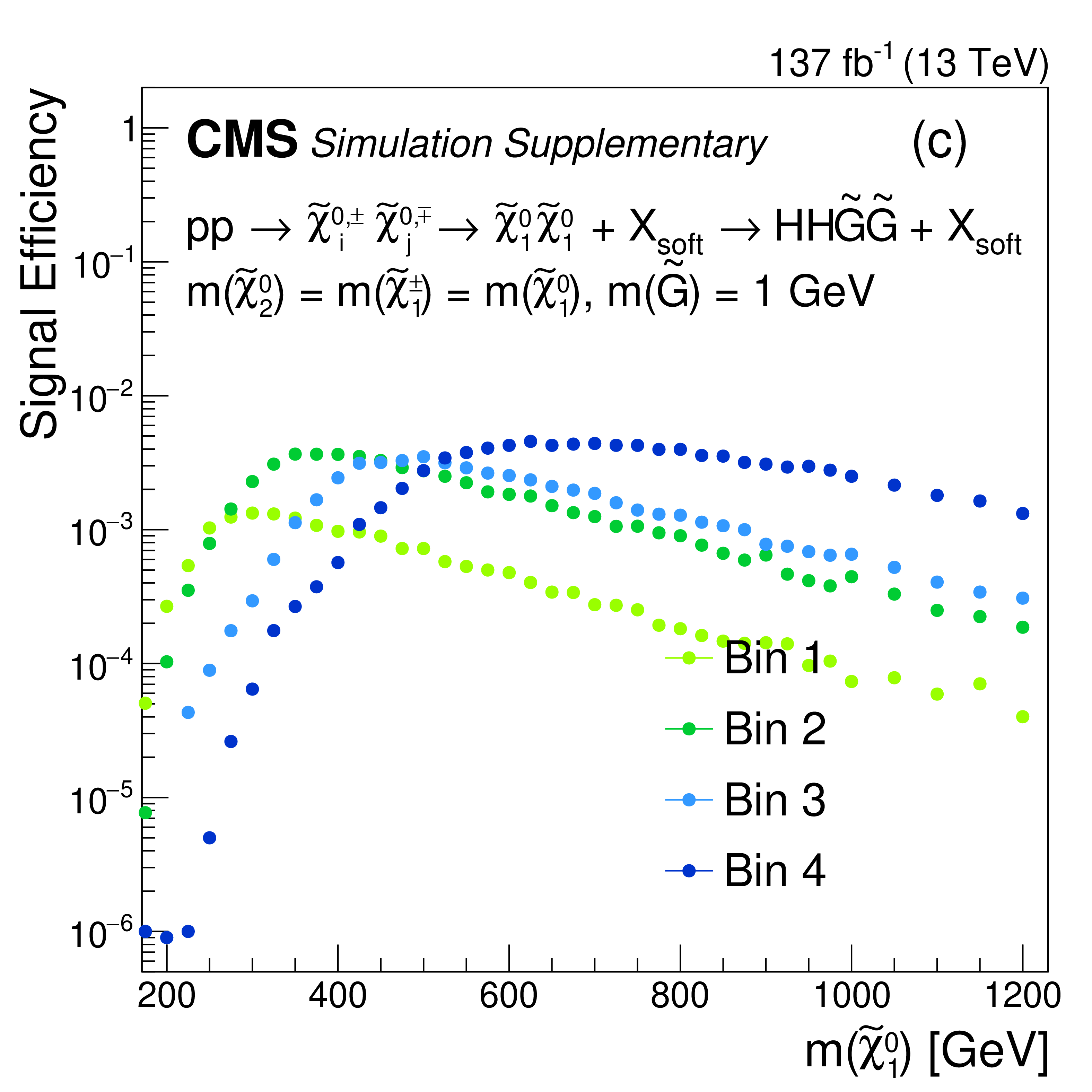
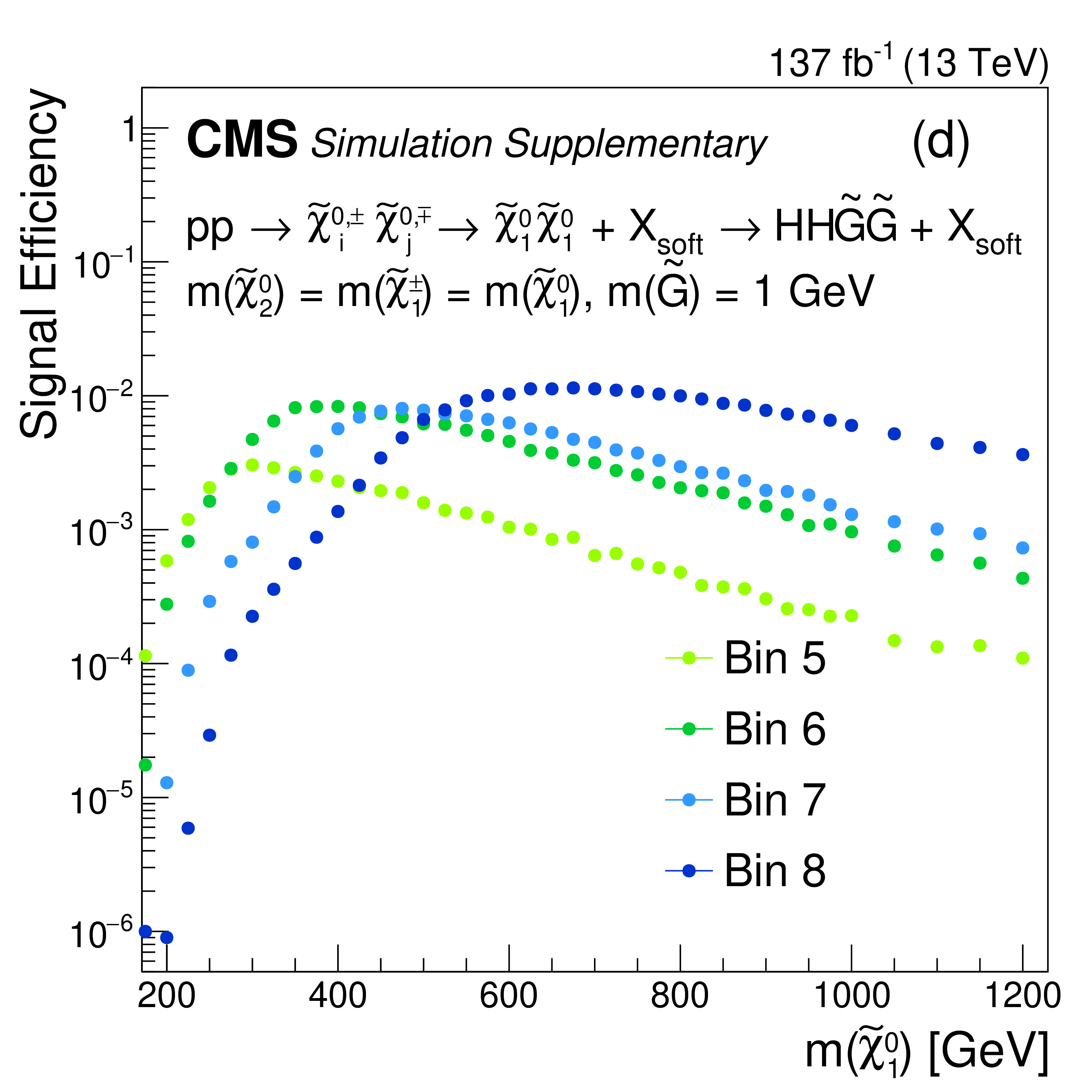
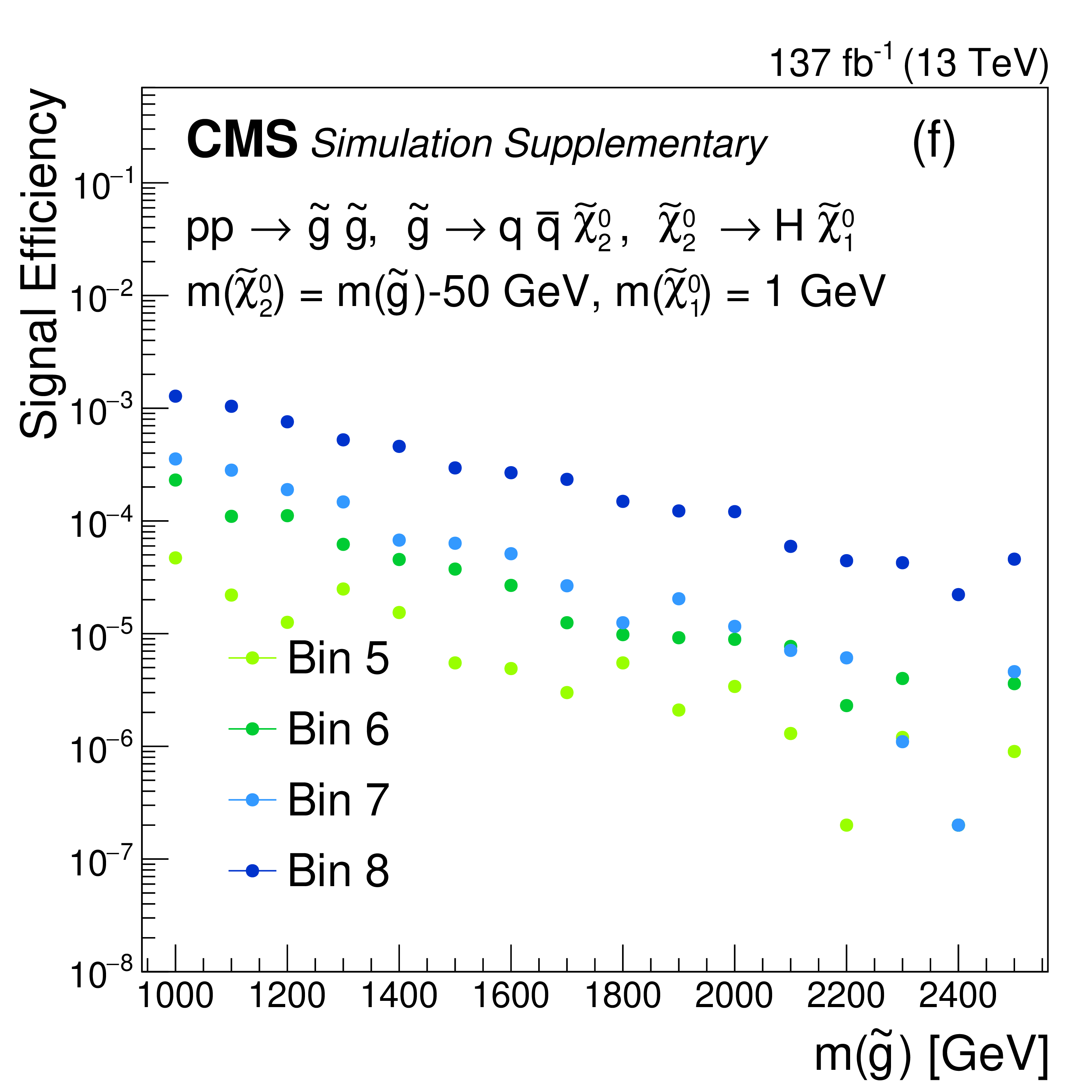
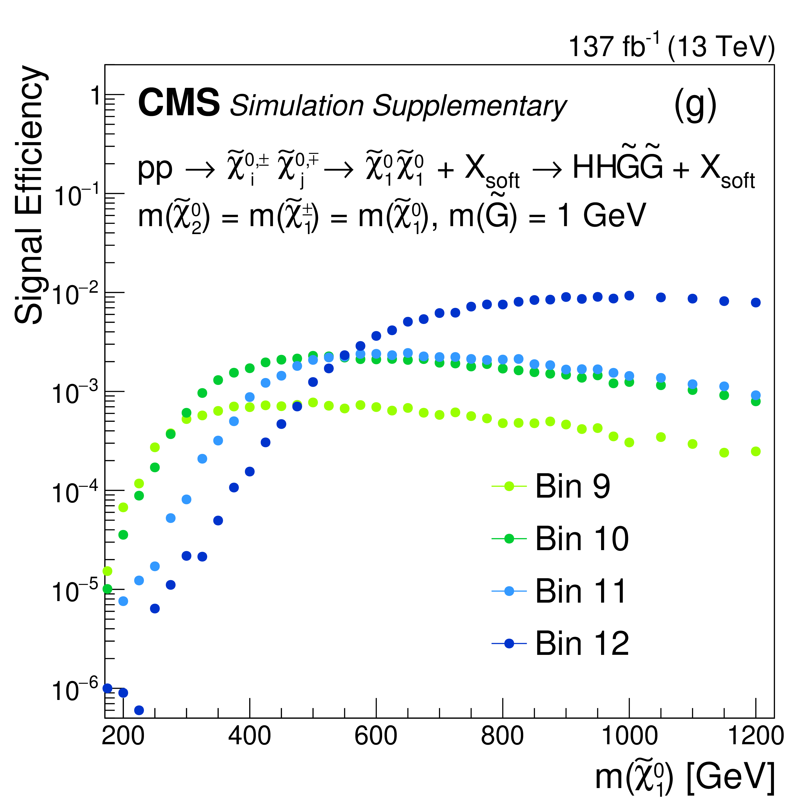
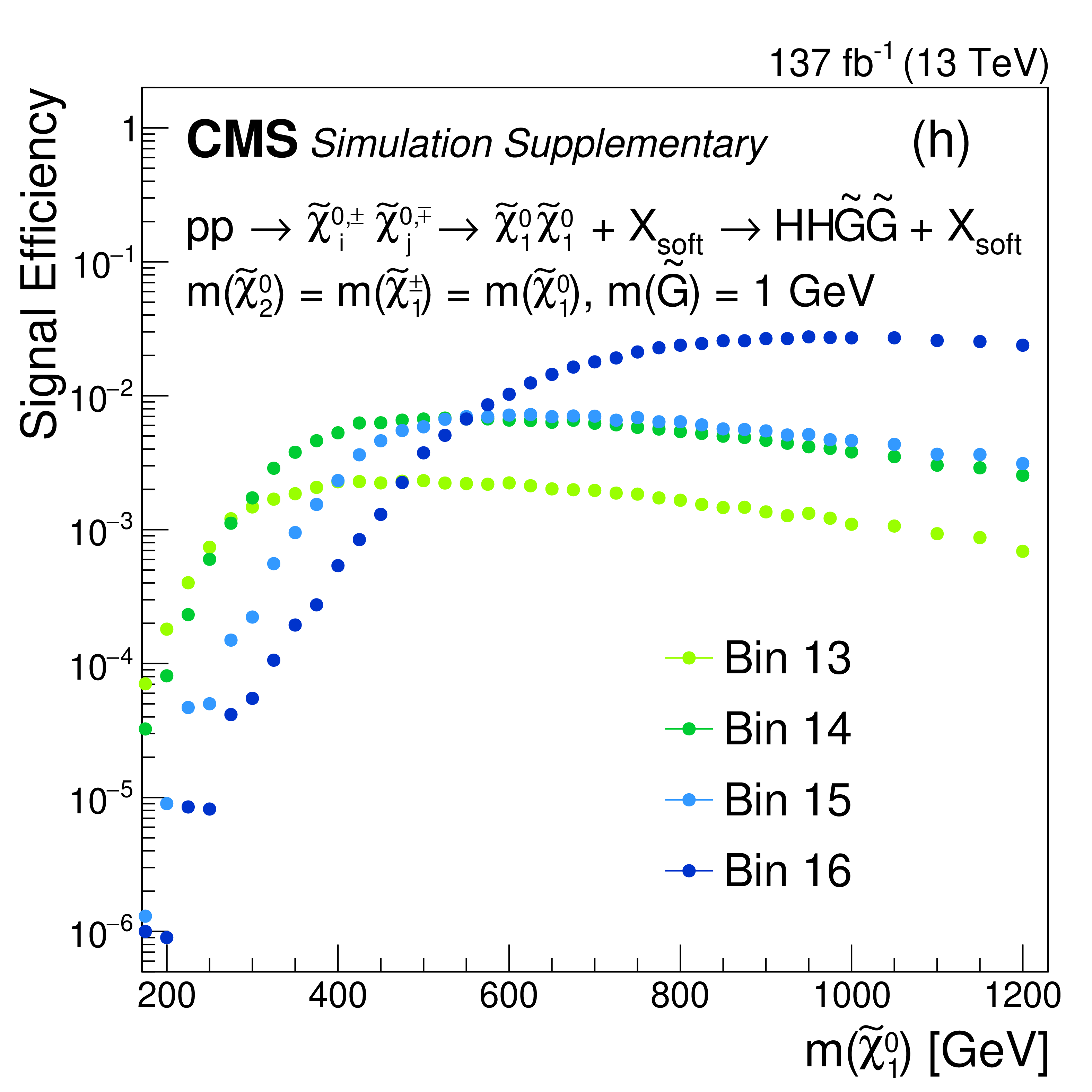
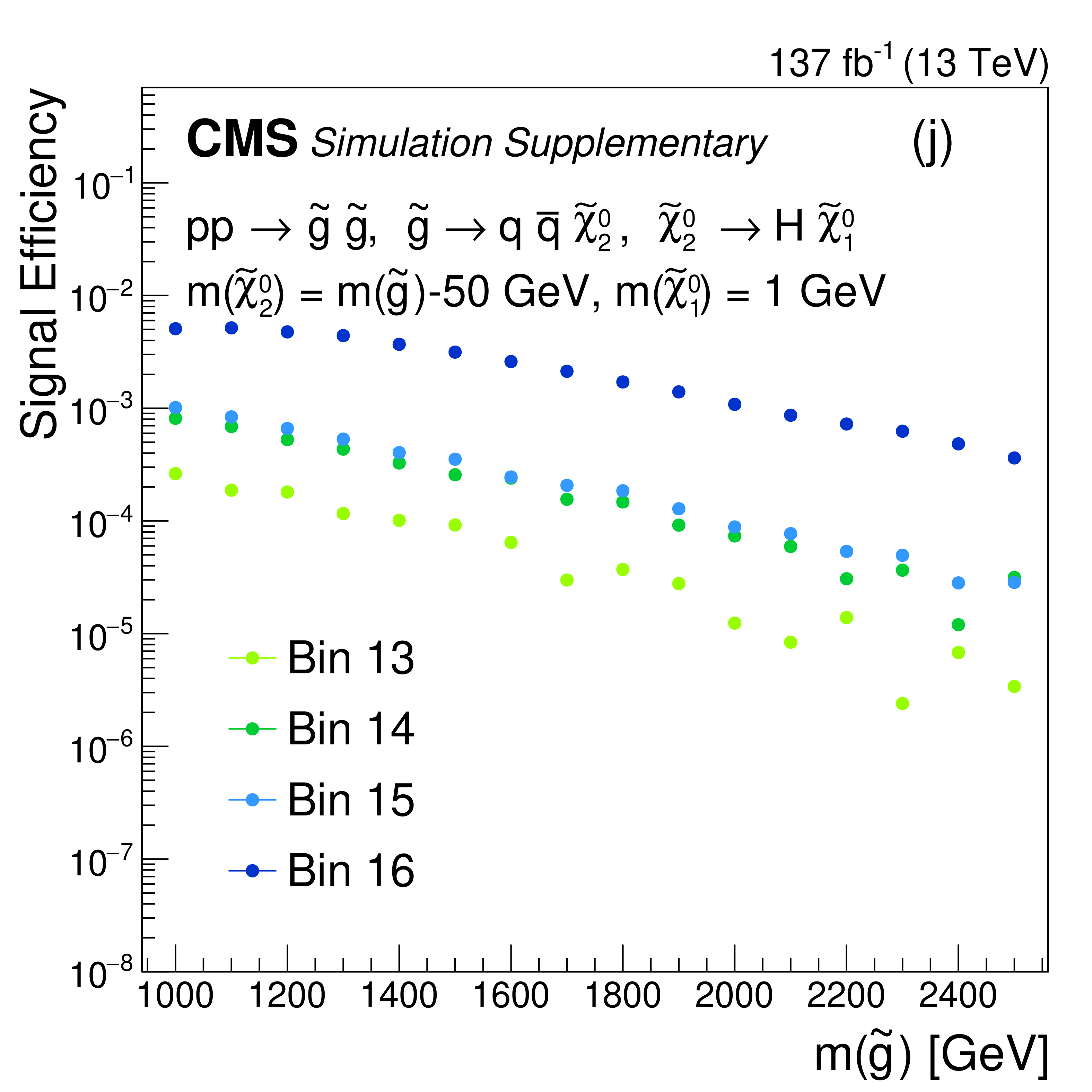
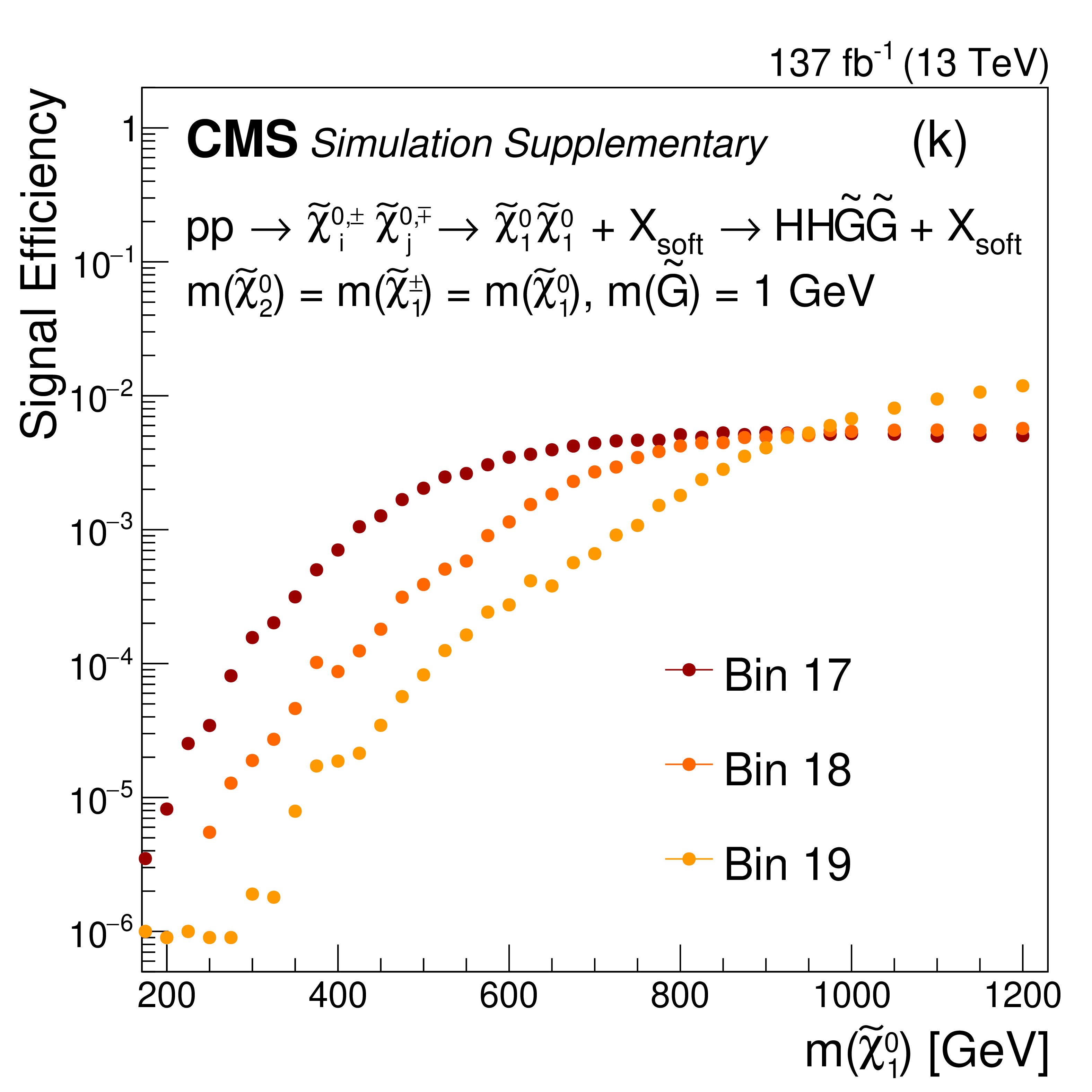
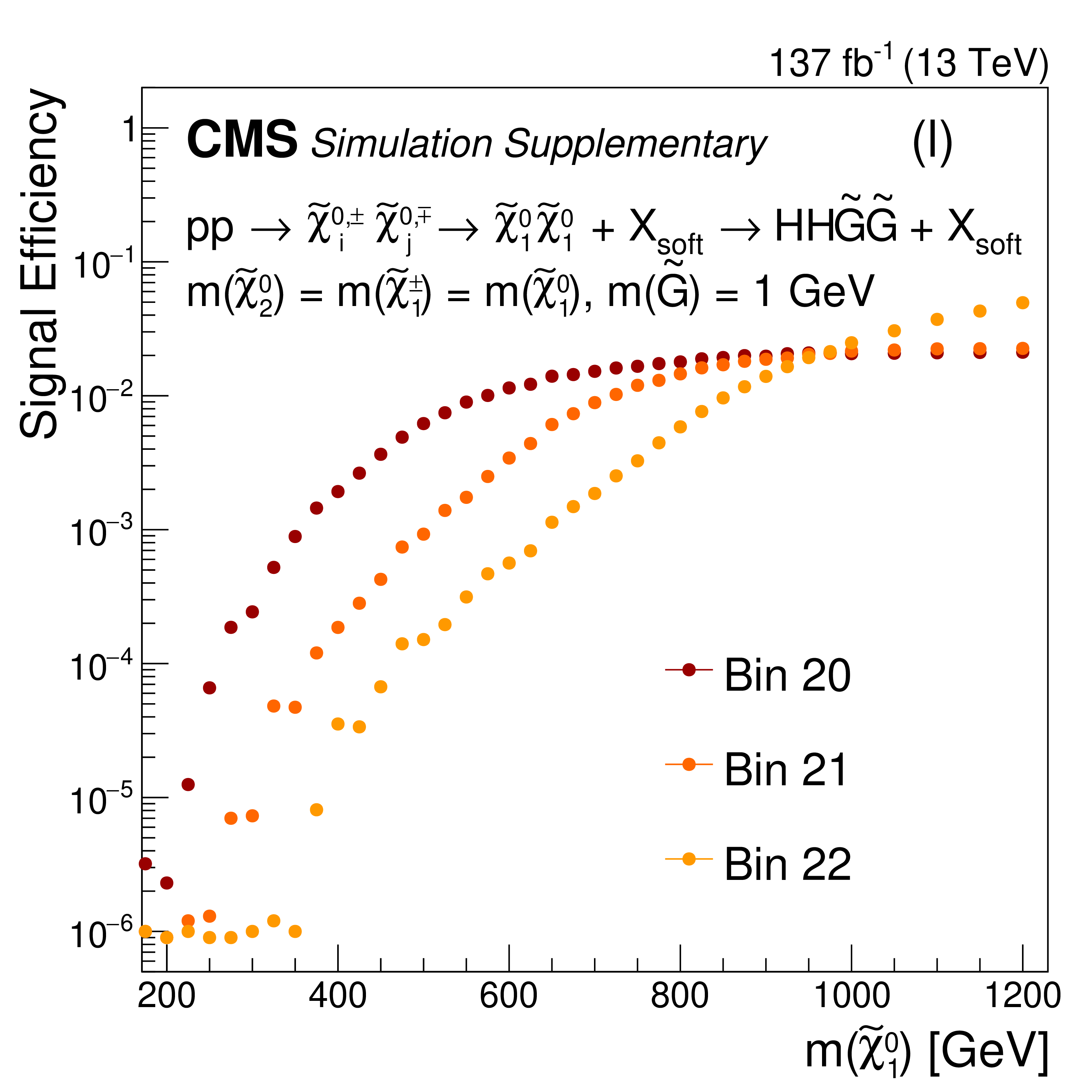
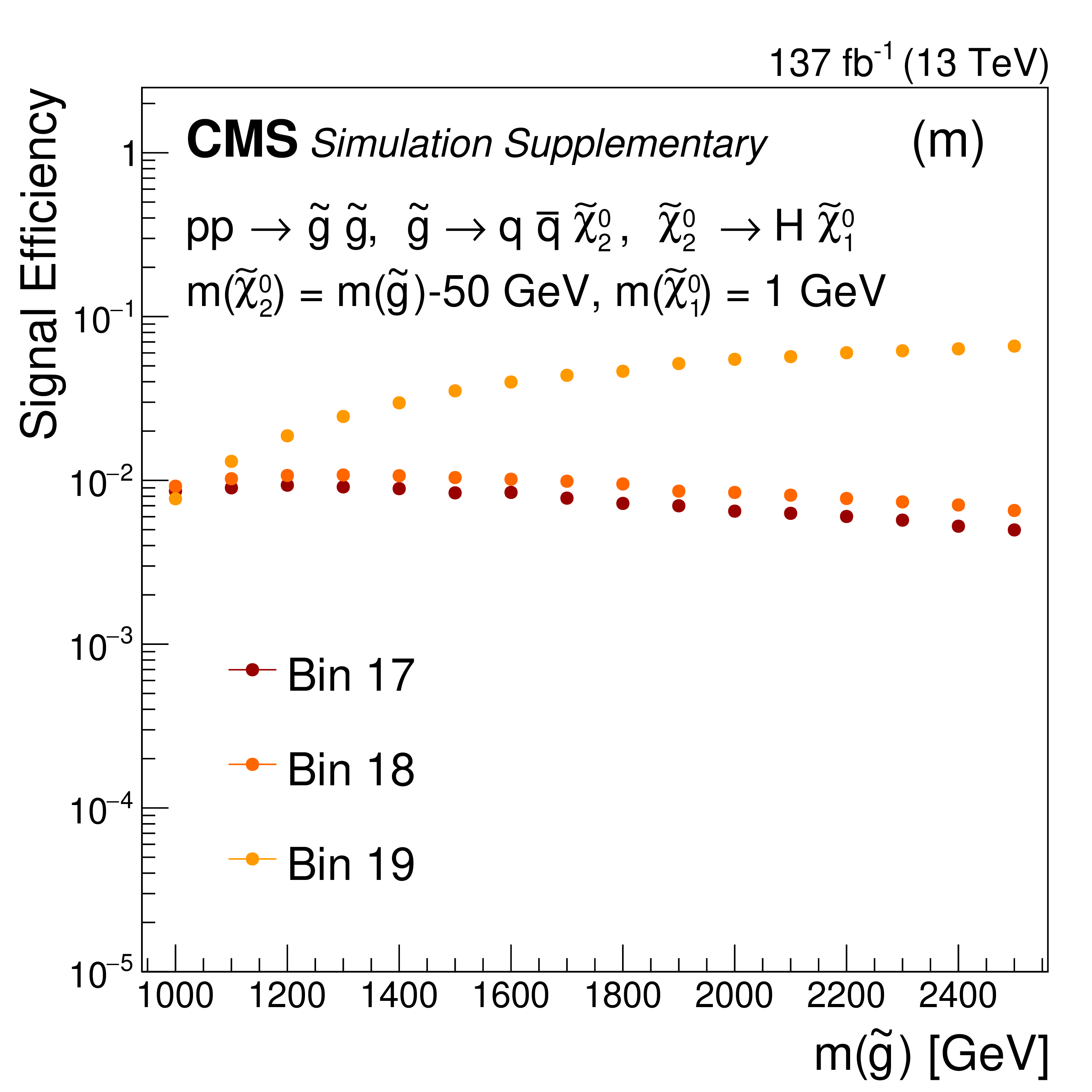
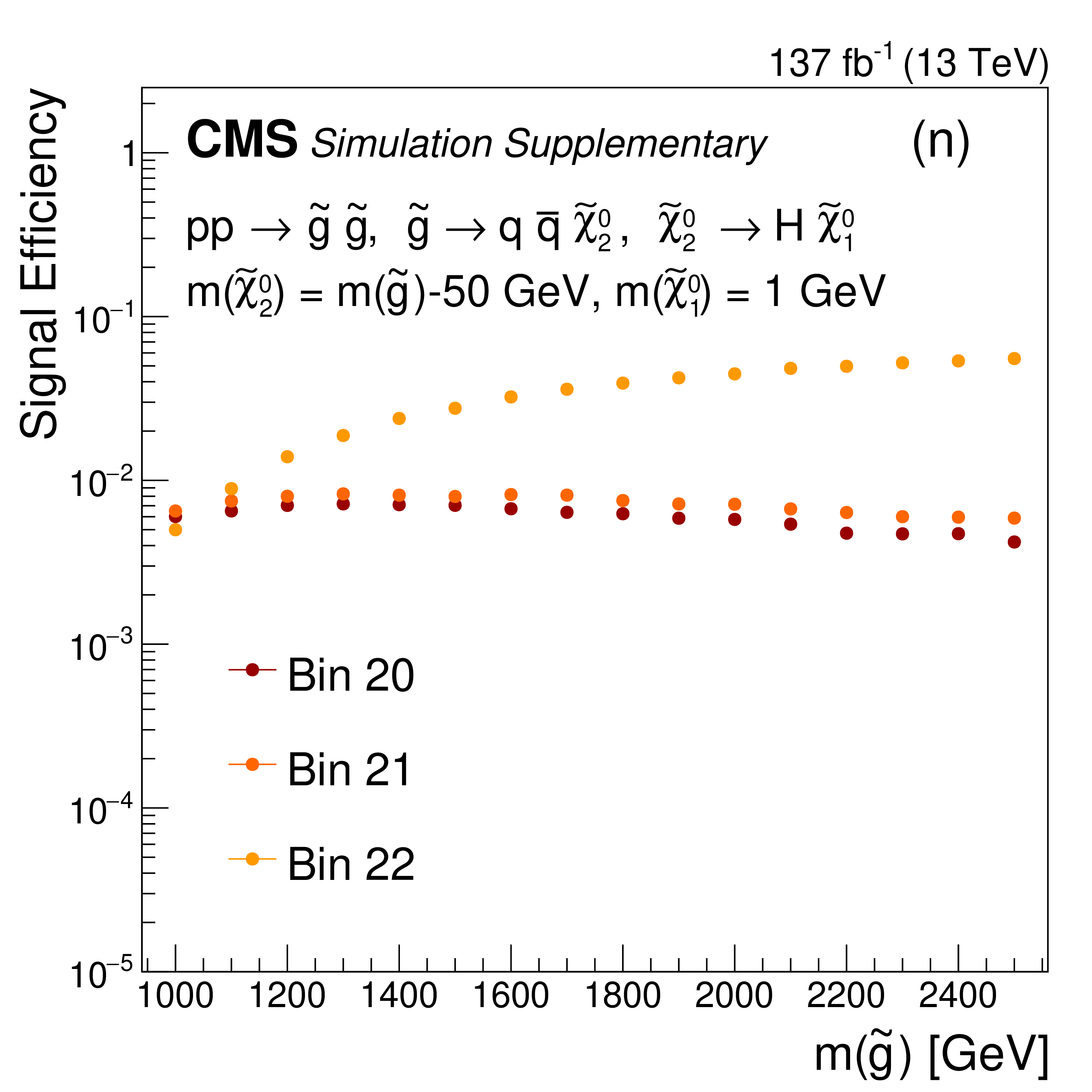
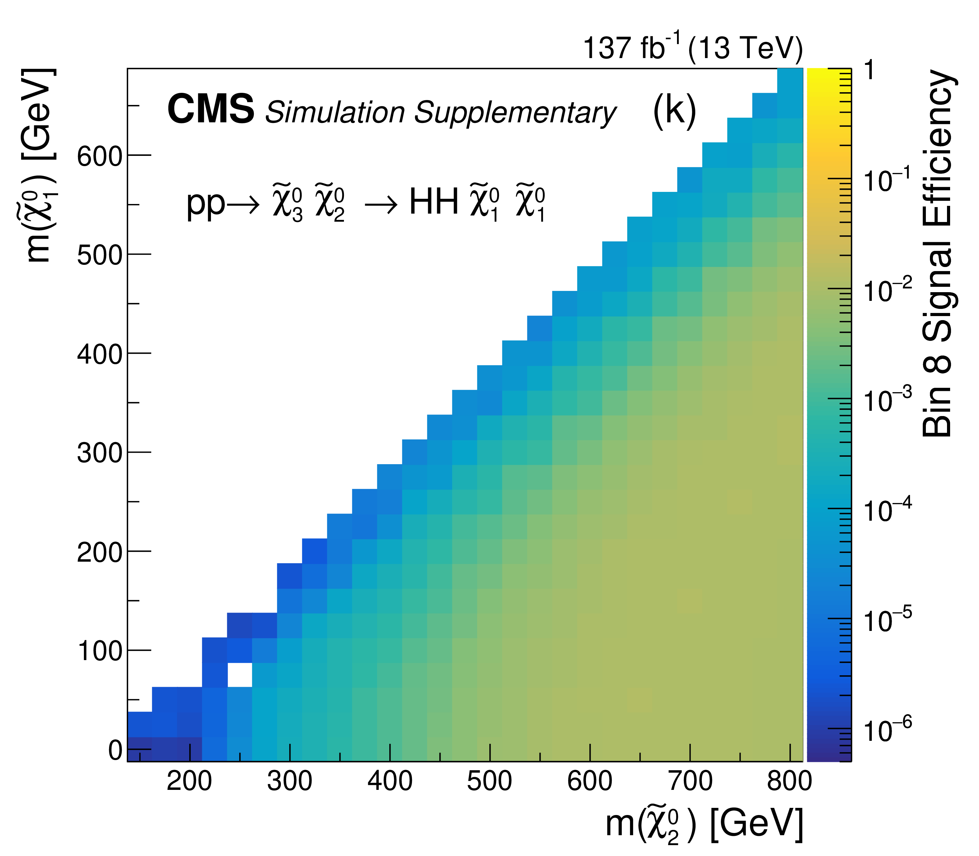
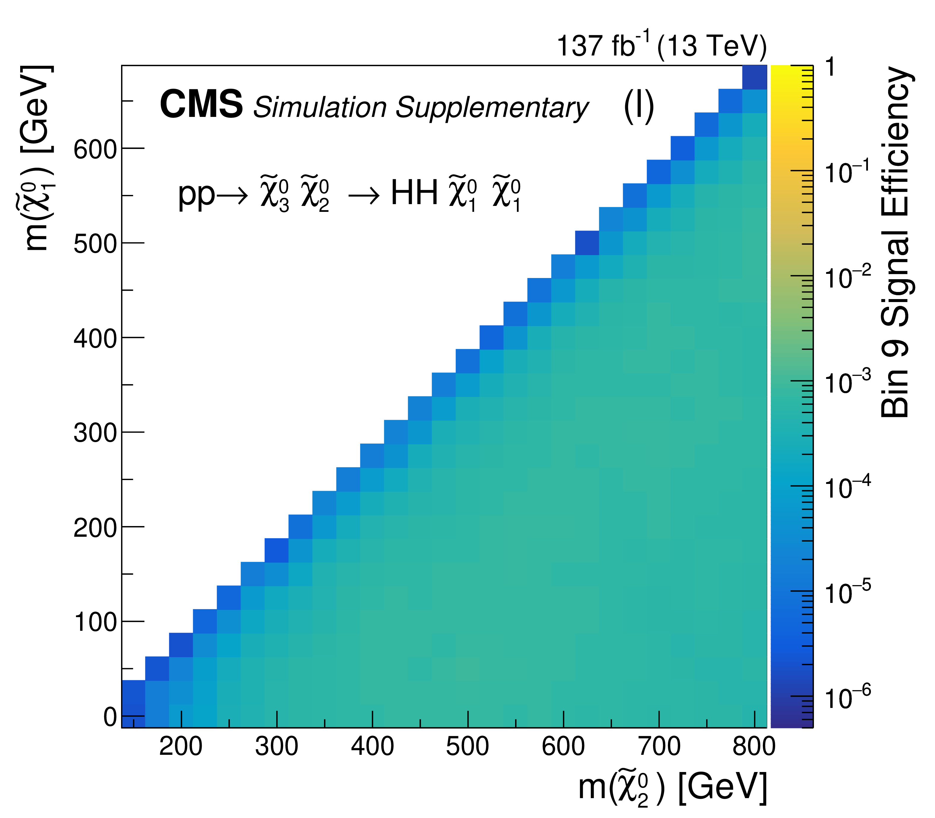
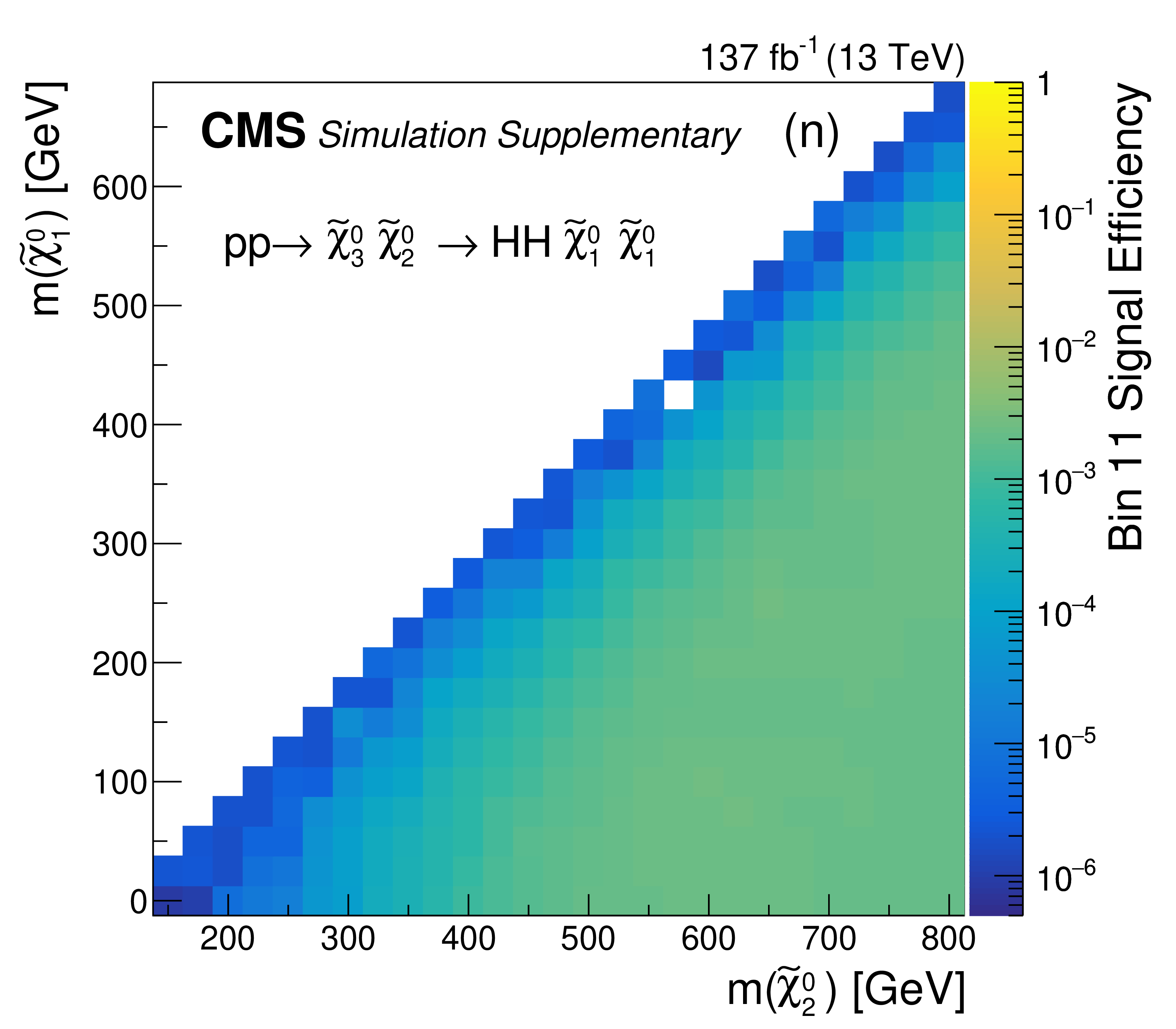
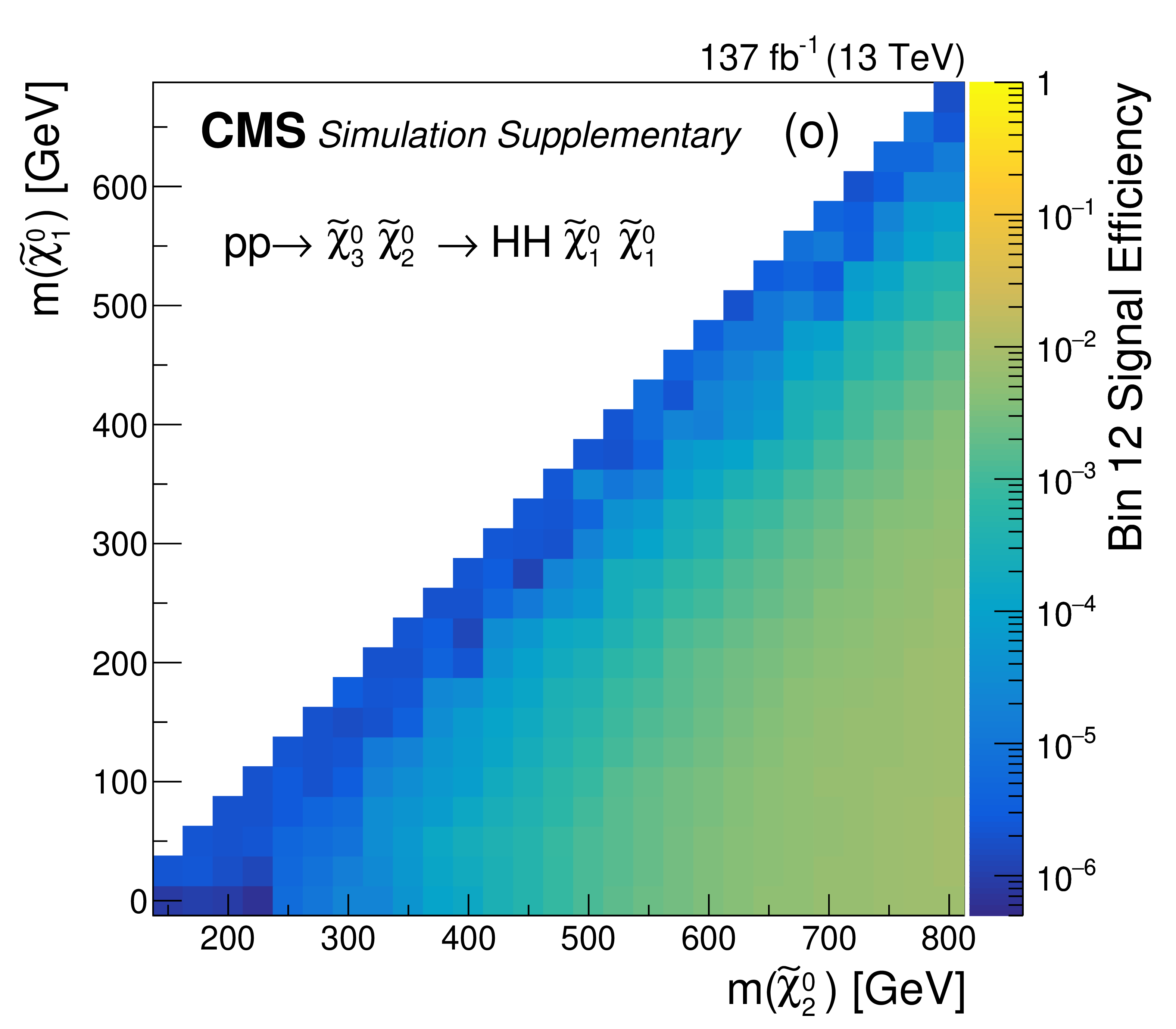
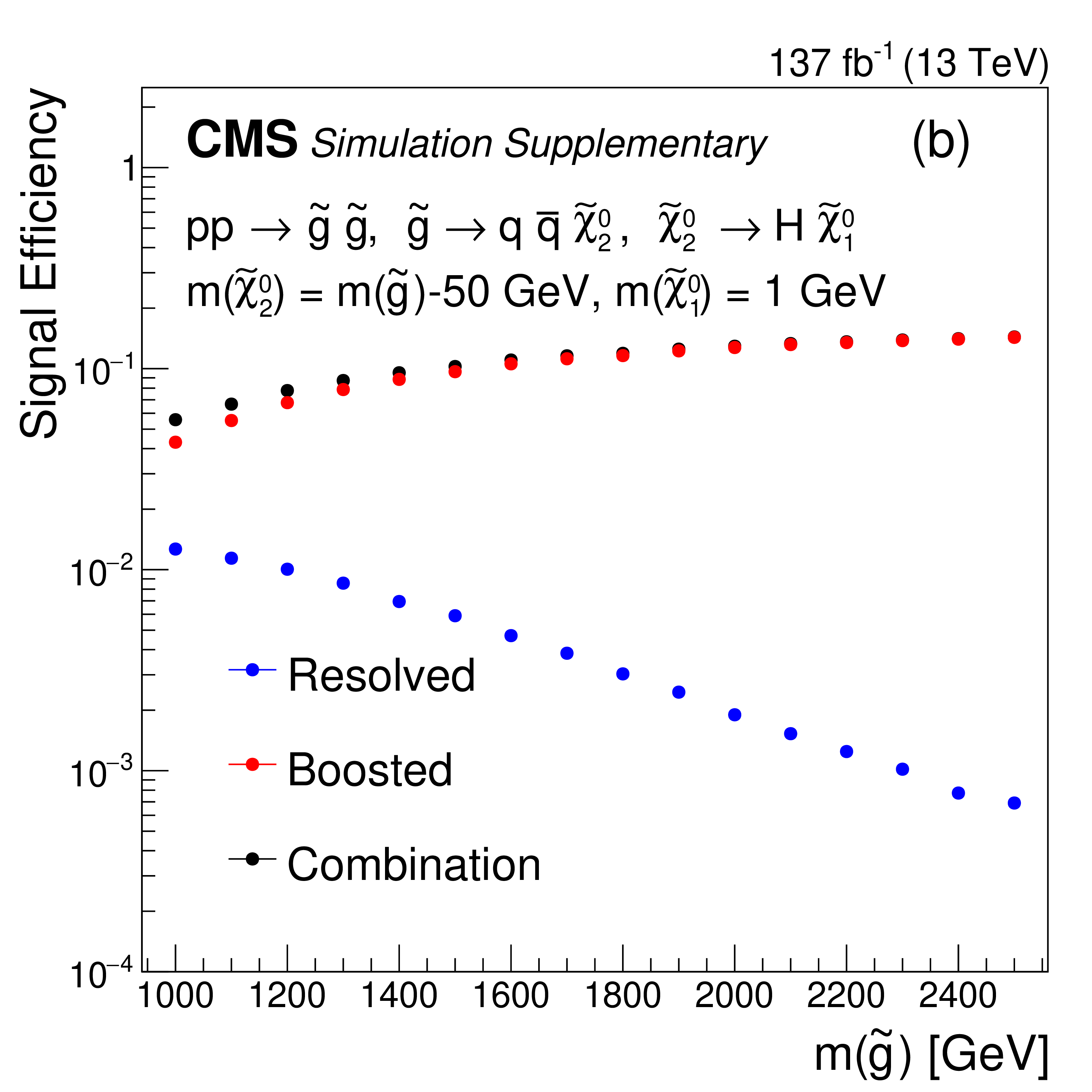
png pdf	Additional Figure 3: Efficiency by signal region for the TChiHH-G model, $\tilde{\chi}^0_1 \tilde{\chi}^0_1 \to \mathrm{H} \mathrm{H} \tilde{\mathrm{G}} \tilde{\mathrm{G}} $ (left two columns), or the T5HH model, ${\mathrm{\widetilde{g}}} {\mathrm{\widetilde{g}}} \to \mathrm{q} \mathrm{\bar{q}} \mathrm{H} \mathrm{H} \tilde{\chi}^0_1 \tilde{\chi}^0_1 $ (right two columns). In the first row (a, b) are shown the resolved-only topology, bins 1-16 (blue), the boosted-only topology, bins 17-22 (red), and all bins 1-22 (black). In the remaining rows are shown: (c, e) bins 1-4; (d, f) bins 5-8; (g, h) bins 9-12; (i, j) bins 13-16; (k, m) bins 17-19; and (l, n) bins 20-22. The data within plots are given, in increasing order of bin number, by colors ranging from light green to blue (c-j) or red to light orange (k-n). The SR indexing is given in Tables 4 and 5 of the paper. The denominator for the efficiency calculation of the TChiHH-G model includes only $\mathrm{H} \to \mathrm{b} \mathrm{\bar{b}} $ decays (for all SRs).
png pdf root	Additional Figure 3-a: Efficiency by signal region for the TChiHH-G model, $\tilde{\chi}^0_1 \tilde{\chi}^0_1 \to \mathrm{H} \mathrm{H} \tilde{\mathrm{G}} \tilde{\mathrm{G}} $. In this plot are shown the resolved-only topology, bins 1-16 (blue), the boosted-only topology, bins 17-22 (red), and all bins 1-22 (black). The SR indexing is given in Tables 4 and 5 of the paper. The denominator for the efficiency calculation includes only $\mathrm{H} \to \mathrm{b} \mathrm{\bar{b}} $ decays (for all SRs).
png pdf root	Additional Figure 3-b: Efficiency by signal region for the T5HH model, ${\mathrm{\widetilde{g}}} {\mathrm{\widetilde{g}}} \to \mathrm{q} \mathrm{\bar{q}} \mathrm{H} \mathrm{H} \tilde{\chi}^0_1 \tilde{\chi}^0_1 $. In this plot are shown the resolved-only topology, bins 1-16 (blue), the boosted-only topology, bins 17-22 (red), and all bins 1-22 (black).
png pdf root	Additional Figure 3-c: Efficiency by signal region for the TChiHH-G model, $\tilde{\chi}^0_1 \tilde{\chi}^0_1 \to \mathrm{H} \mathrm{H} \tilde{\mathrm{G}} \tilde{\mathrm{G}} $. In this plot are shown bins 1-4. The data within the plot are given, in increasing order of bin number, by colors ranging from light green to blue. The SR indexing is given in Tables 4 and 5 of the paper. The denominator for the efficiency calculation includes only $\mathrm{H} \to \mathrm{b} \mathrm{\bar{b}} $ decays (for all SRs).
png pdf root	Additional Figure 3-d: Efficiency by signal region for the TChiHH-G model, $\tilde{\chi}^0_1 \tilde{\chi}^0_1 \to \mathrm{H} \mathrm{H} \tilde{\mathrm{G}} \tilde{\mathrm{G}} $. In this plot are shown bins 5-8. The data within the plot are given, in increasing order of bin number, by colors ranging from light green to blue. The SR indexing is given in Tables 4 and 5 of the paper. The denominator for the efficiency calculation includes only $\mathrm{H} \to \mathrm{b} \mathrm{\bar{b}} $ decays (for all SRs).
png pdf root	Additional Figure 3-e: Efficiency by signal region for the T5HH model, ${\mathrm{\widetilde{g}}} {\mathrm{\widetilde{g}}} \to \mathrm{q} \mathrm{\bar{q}} \mathrm{H} \mathrm{H} \tilde{\chi}^0_1 \tilde{\chi}^0_1 $. In this plot are shown bins 1-4. The data within the plot are given, in increasing order of bin number, by colors ranging from light green to blue. The SR indexing is given in Tables 4 and 5 of the paper.
png pdf root	Additional Figure 3-f: Efficiency by signal region for the T5HH model, ${\mathrm{\widetilde{g}}} {\mathrm{\widetilde{g}}} \to \mathrm{q} \mathrm{\bar{q}} \mathrm{H} \mathrm{H} \tilde{\chi}^0_1 \tilde{\chi}^0_1 $. In this plot are shown bins 5-8. The data within the plot are given, in increasing order of bin number, by colors ranging from light green to blue. The SR indexing is given in Tables 4 and 5 of the paper.
png pdf root	Additional Figure 3-g: Efficiency by signal region for the TChiHH-G model, $\tilde{\chi}^0_1 \tilde{\chi}^0_1 \to \mathrm{H} \mathrm{H} \tilde{\mathrm{G}} \tilde{\mathrm{G}} $. In this plot are shown bins 9-12. The data within the plot are given, in increasing order of bin number, by colors ranging from light green to bluee. The SR indexing is given in Tables 4 and 5 of the paper. The denominator for the efficiency calculation includes only $\mathrm{H} \to \mathrm{b} \mathrm{\bar{b}} $ decays (for all SRs).
png pdf root	Additional Figure 3-h: Efficiency by signal region for the TChiHH-G model, $\tilde{\chi}^0_1 \tilde{\chi}^0_1 \to \mathrm{H} \mathrm{H} \tilde{\mathrm{G}} \tilde{\mathrm{G}} $. In this plot are shown bins 13-16. The data within the plot are given, in increasing order of bin number, by colors ranging from light green to blue. The SR indexing is given in Tables 4 and 5 of the paper. The denominator for the efficiency calculation includes only $\mathrm{H} \to \mathrm{b} \mathrm{\bar{b}} $ decays (for all SRs).
png pdf root	Additional Figure 3-i: Efficiency by signal region for the T5HH model, ${\mathrm{\widetilde{g}}} {\mathrm{\widetilde{g}}} \to \mathrm{q} \mathrm{\bar{q}} \mathrm{H} \mathrm{H} \tilde{\chi}^0_1 \tilde{\chi}^0_1 $. In this plot are shown bins 9-12. The data within the plot are given, in increasing order of bin number, by colors ranging from light green to blue. The SR indexing is given in Tables 4 and 5 of the paper.
png pdf root	Additional Figure 3-j: Efficiency by signal region for the T5HH model, ${\mathrm{\widetilde{g}}} {\mathrm{\widetilde{g}}} \to \mathrm{q} \mathrm{\bar{q}} \mathrm{H} \mathrm{H} \tilde{\chi}^0_1 \tilde{\chi}^0_1 $. In this plot are shown bins 13-16. The data within the plot are given, in increasing order of bin number, by colors ranging from light green to blue. The SR indexing is given in Tables 4 and 5 of the paper.
png pdf root	Additional Figure 3-k: Efficiency by signal region for the TChiHH-G model, $\tilde{\chi}^0_1 \tilde{\chi}^0_1 \to \mathrm{H} \mathrm{H} \tilde{\mathrm{G}} \tilde{\mathrm{G}} $. In this plot are shown bins 17-19. The data within the plot are given, in increasing order of bin number, by colors ranging from red to light orange. The SR indexing is given in Tables 4 and 5 of the paper. The denominator for the efficiency calculation includes only $\mathrm{H} \to \mathrm{b} \mathrm{\bar{b}} $ decays (for all SRs).
png pdf root	Additional Figure 3-l: Efficiency by signal region for the TChiHH-G model, $\tilde{\chi}^0_1 \tilde{\chi}^0_1 \to \mathrm{H} \mathrm{H} \tilde{\mathrm{G}} \tilde{\mathrm{G}} $. In this plot are shown bins 20-22. The data within the plot are given, in increasing order of bin number, by colors ranging from red to light orange. The SR indexing is given in Tables 4 and 5 of the paper. The denominator for the efficiency calculation includes only $\mathrm{H} \to \mathrm{b} \mathrm{\bar{b}} $ decays (for all SRs).
png pdf root	Additional Figure 3-m: Efficiency by signal region for the T5HH model, ${\mathrm{\widetilde{g}}} {\mathrm{\widetilde{g}}} \to \mathrm{q} \mathrm{\bar{q}} \mathrm{H} \mathrm{H} \tilde{\chi}^0_1 \tilde{\chi}^0_1 $. In this plot are shown bins 17-19. The data within the plot are given, in increasing order of bin number, by colors ranging from red to light orange. The SR indexing is given in Tables 4 and 5 of the paper.
png pdf root	Additional Figure 3-n: Efficiency by signal region for the T5HH model, ${\mathrm{\widetilde{g}}} {\mathrm{\widetilde{g}}} \to \mathrm{q} \mathrm{\bar{q}} \mathrm{H} \mathrm{H} \tilde{\chi}^0_1 \tilde{\chi}^0_1 $. In this plot are shown bins 20-22. The data within the plot are given, in increasing order of bin number, by colors ranging from red to light orange. The SR indexing is given in Tables 4 and 5 of the paper.
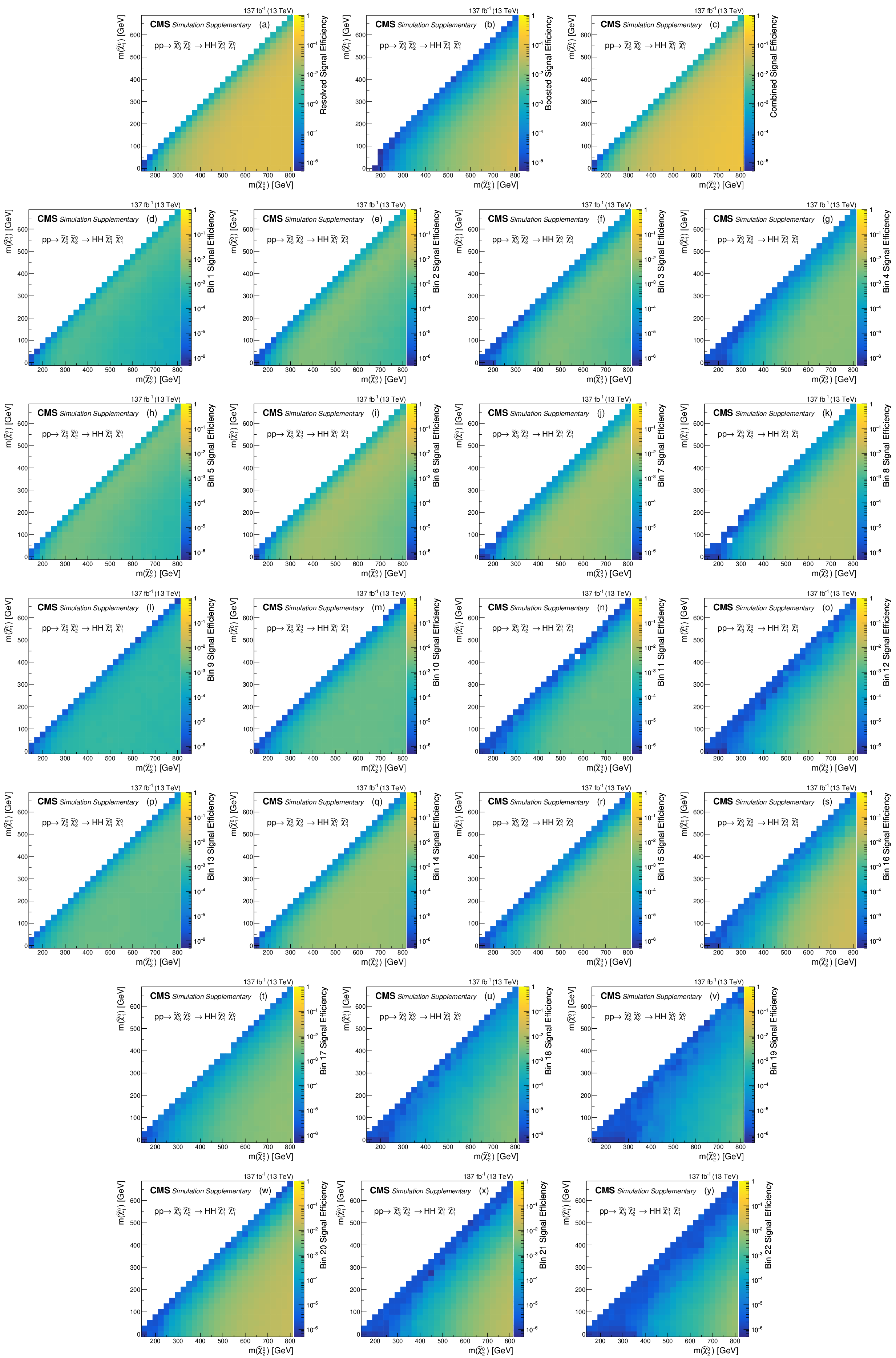
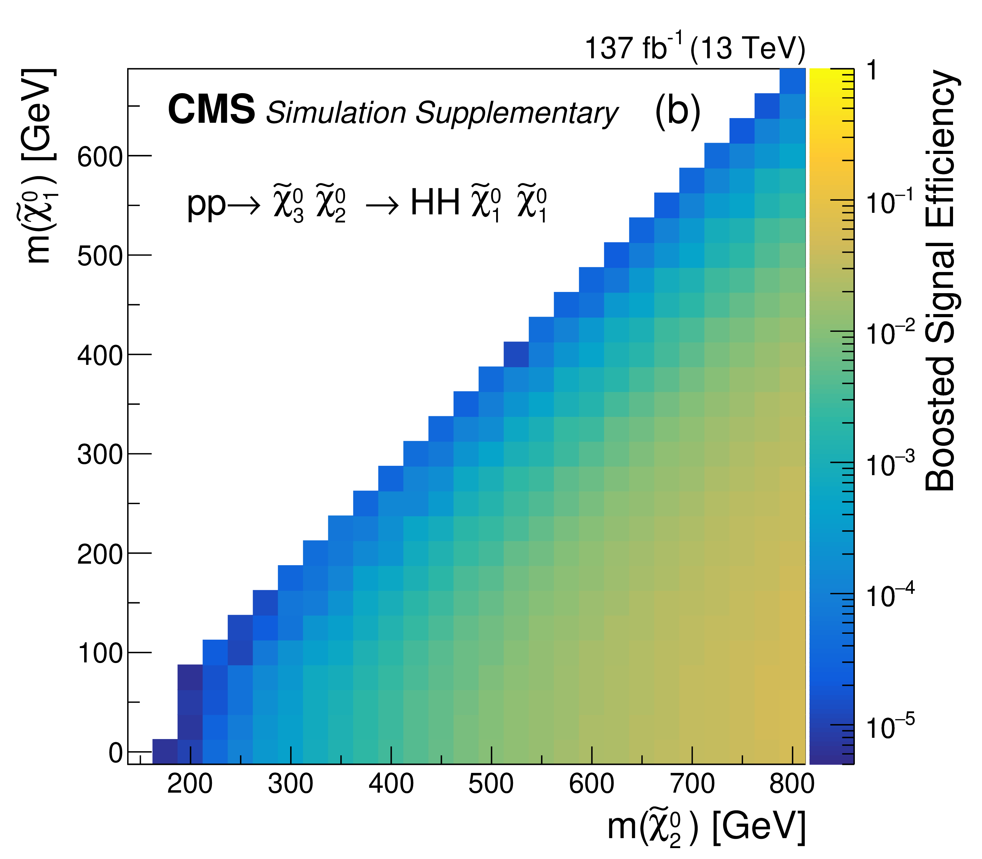
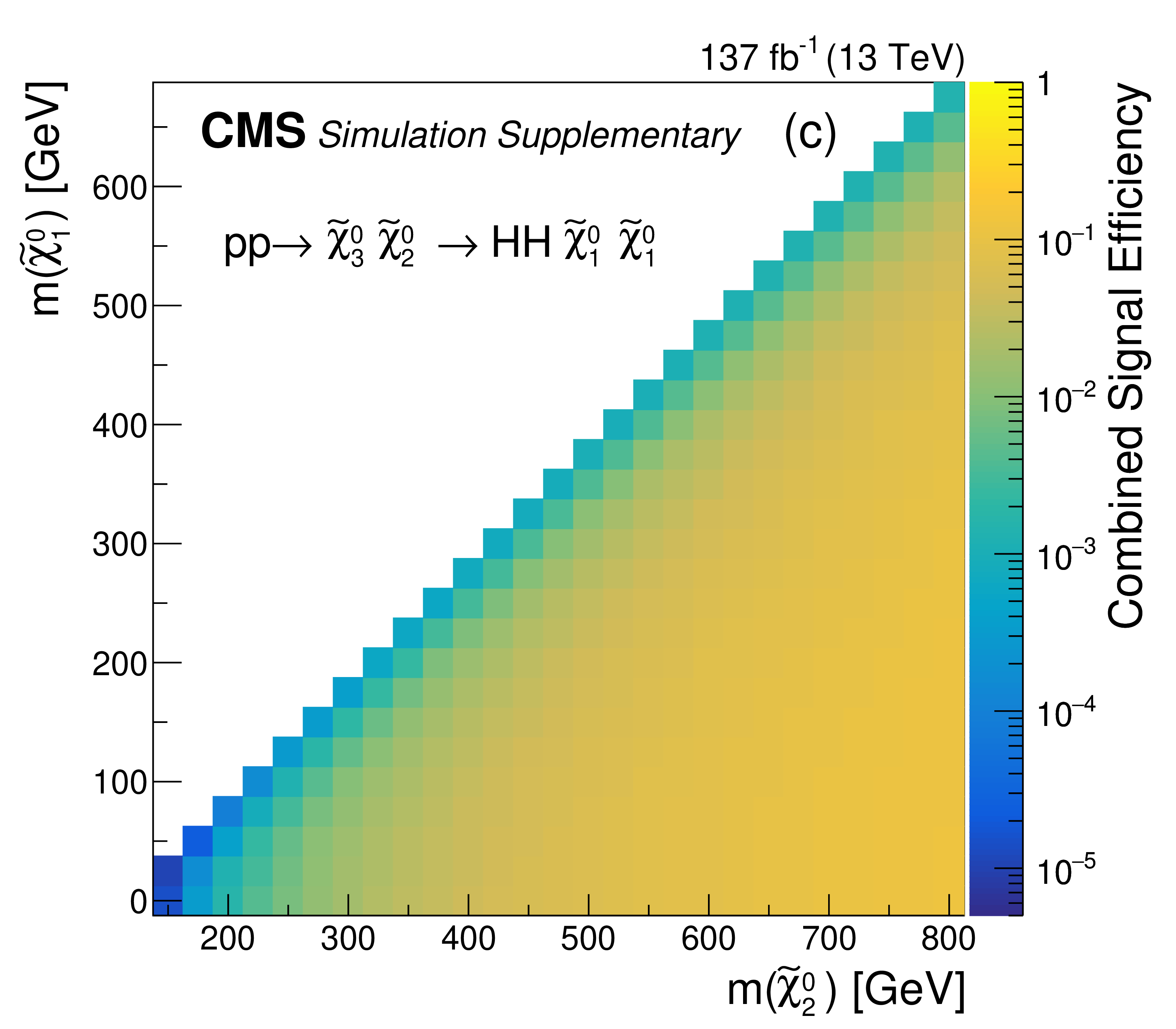
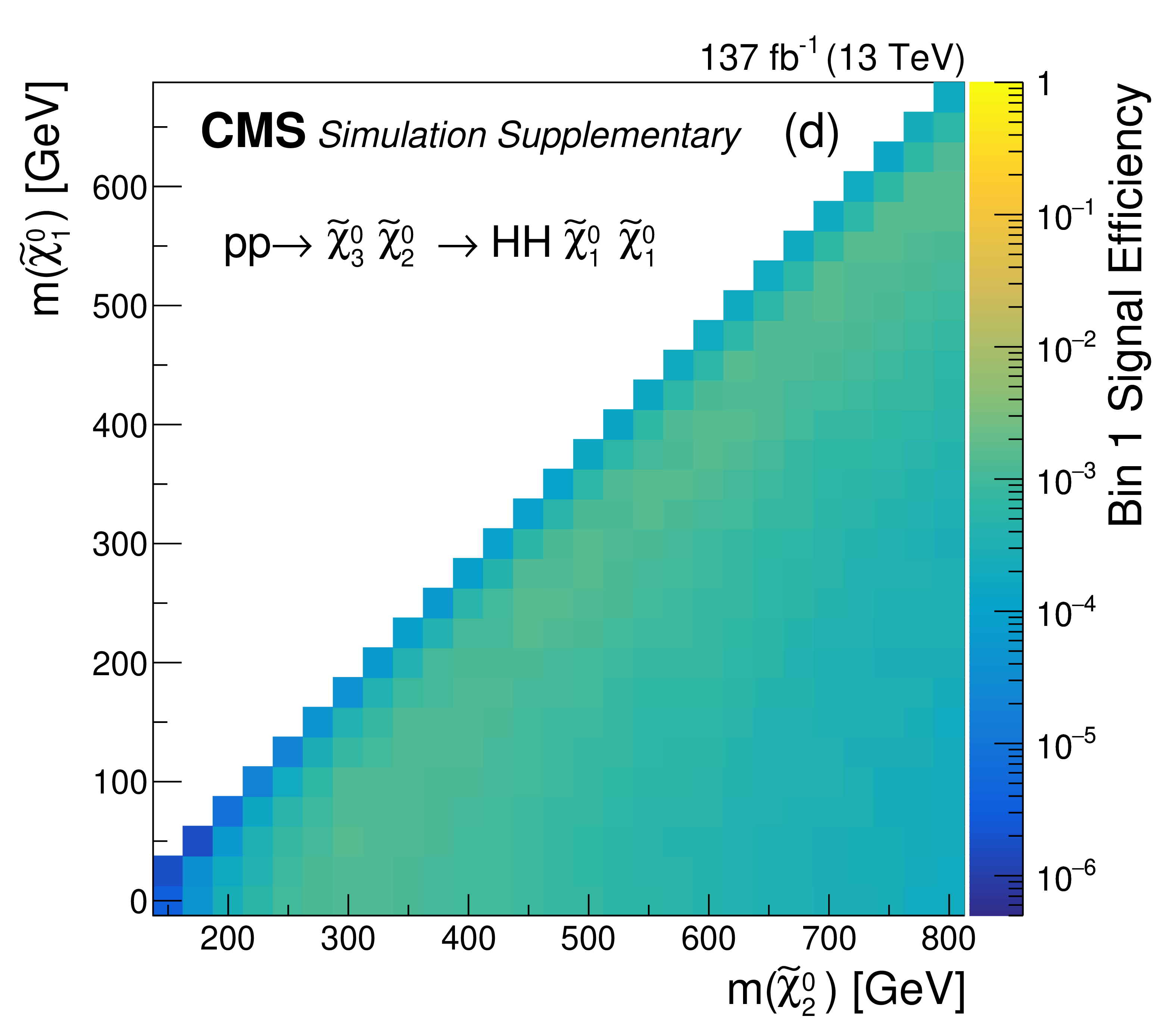
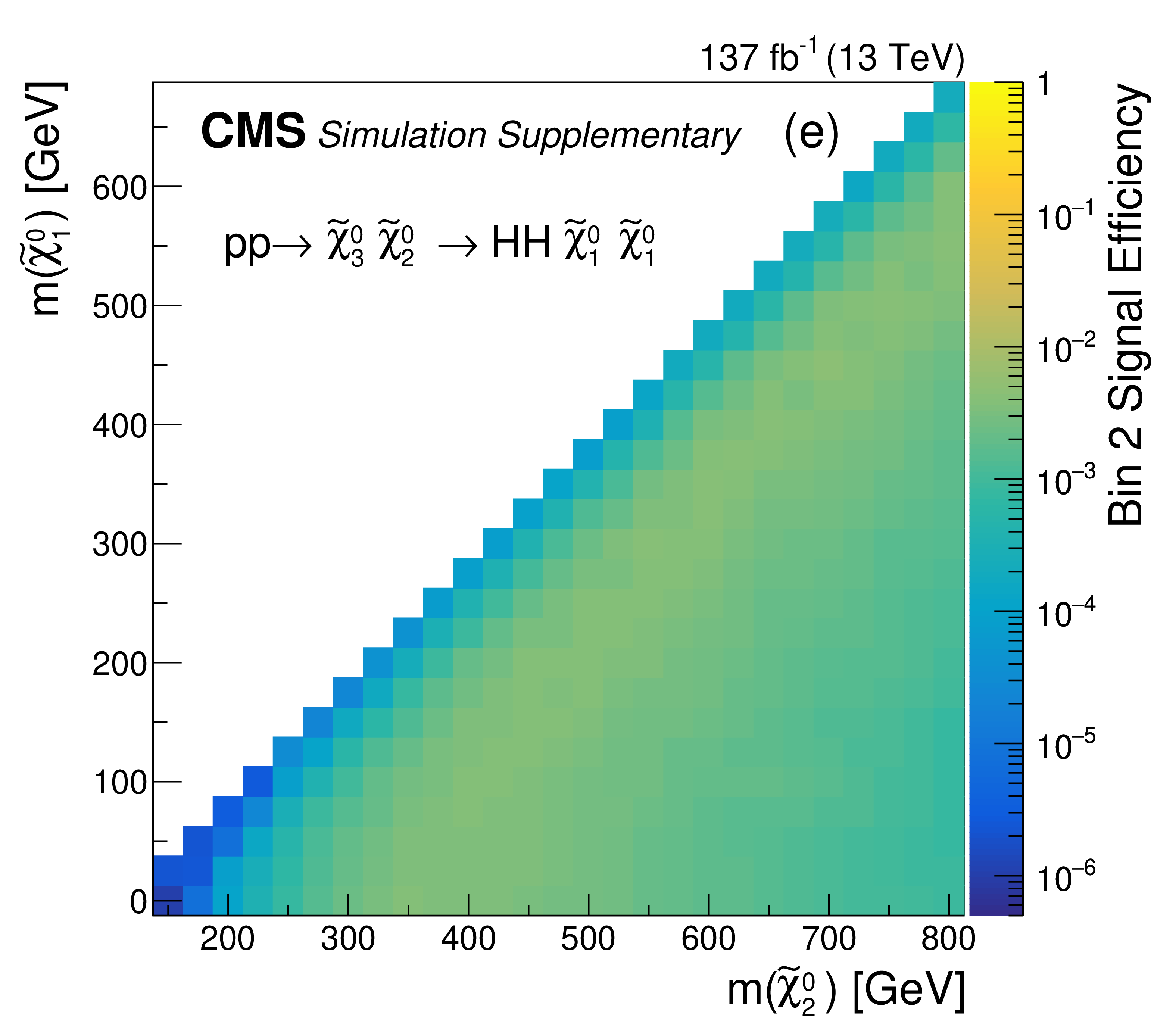
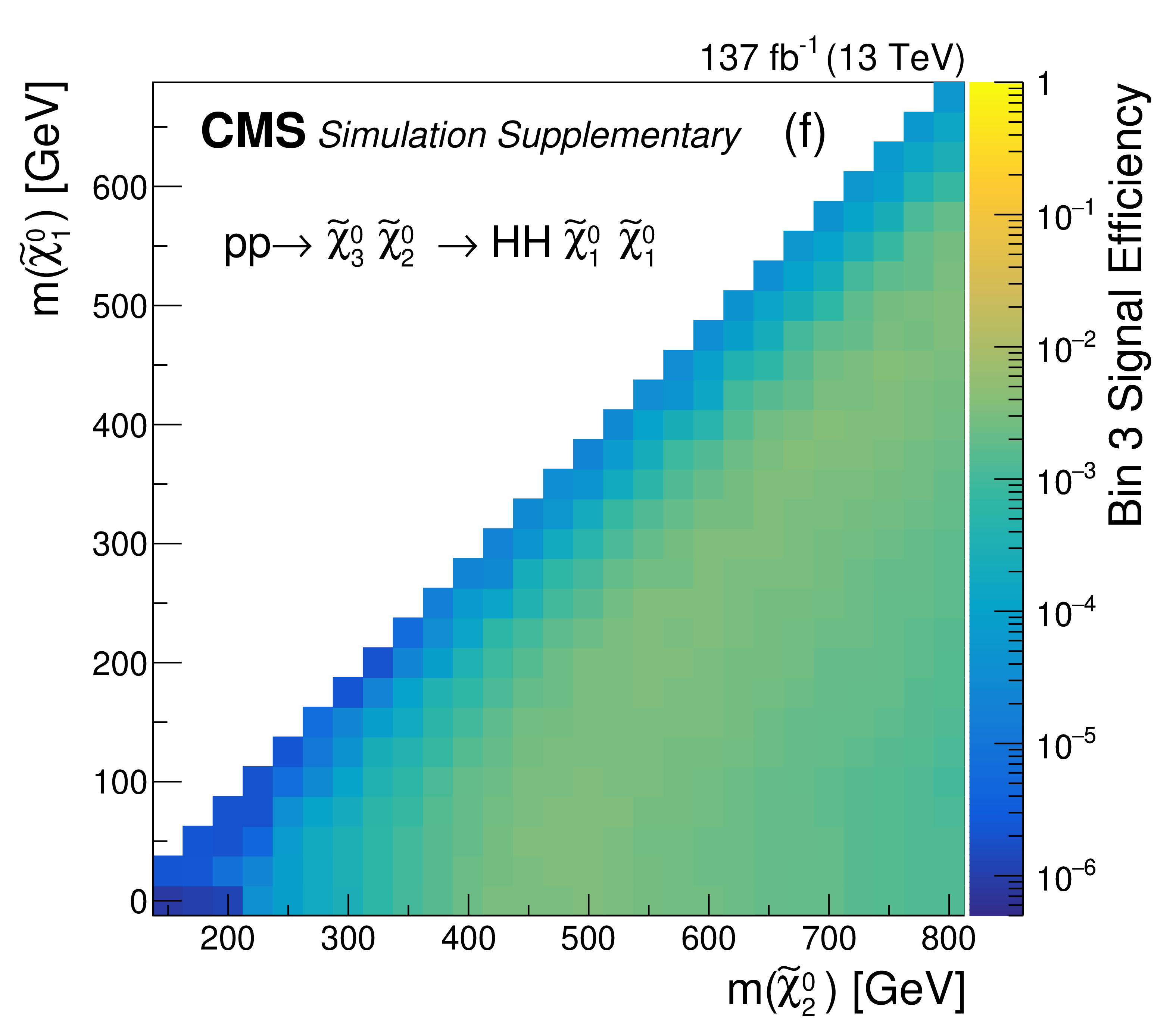
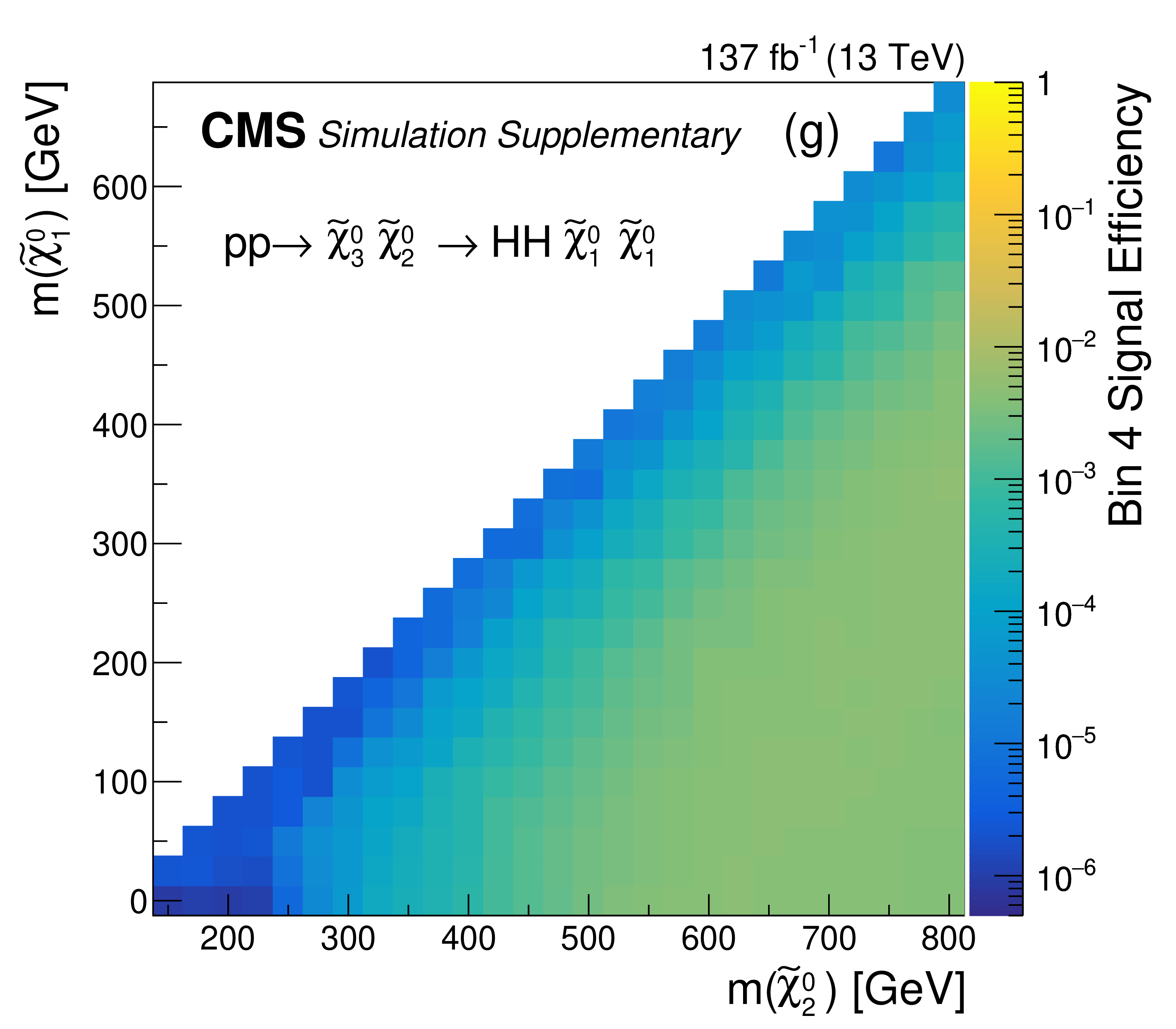
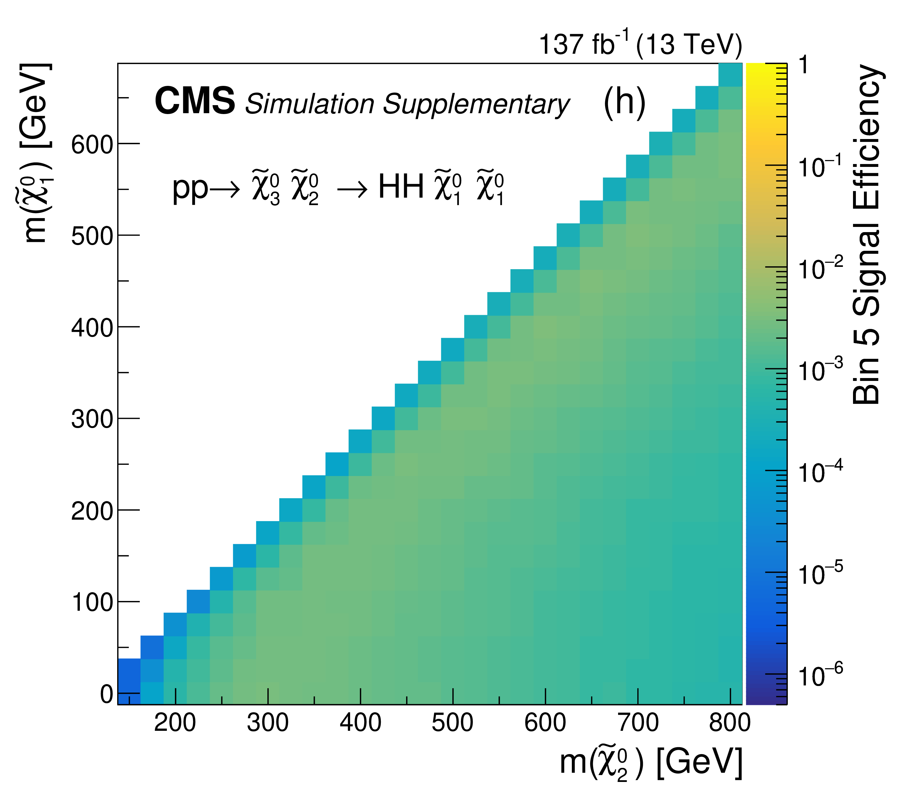
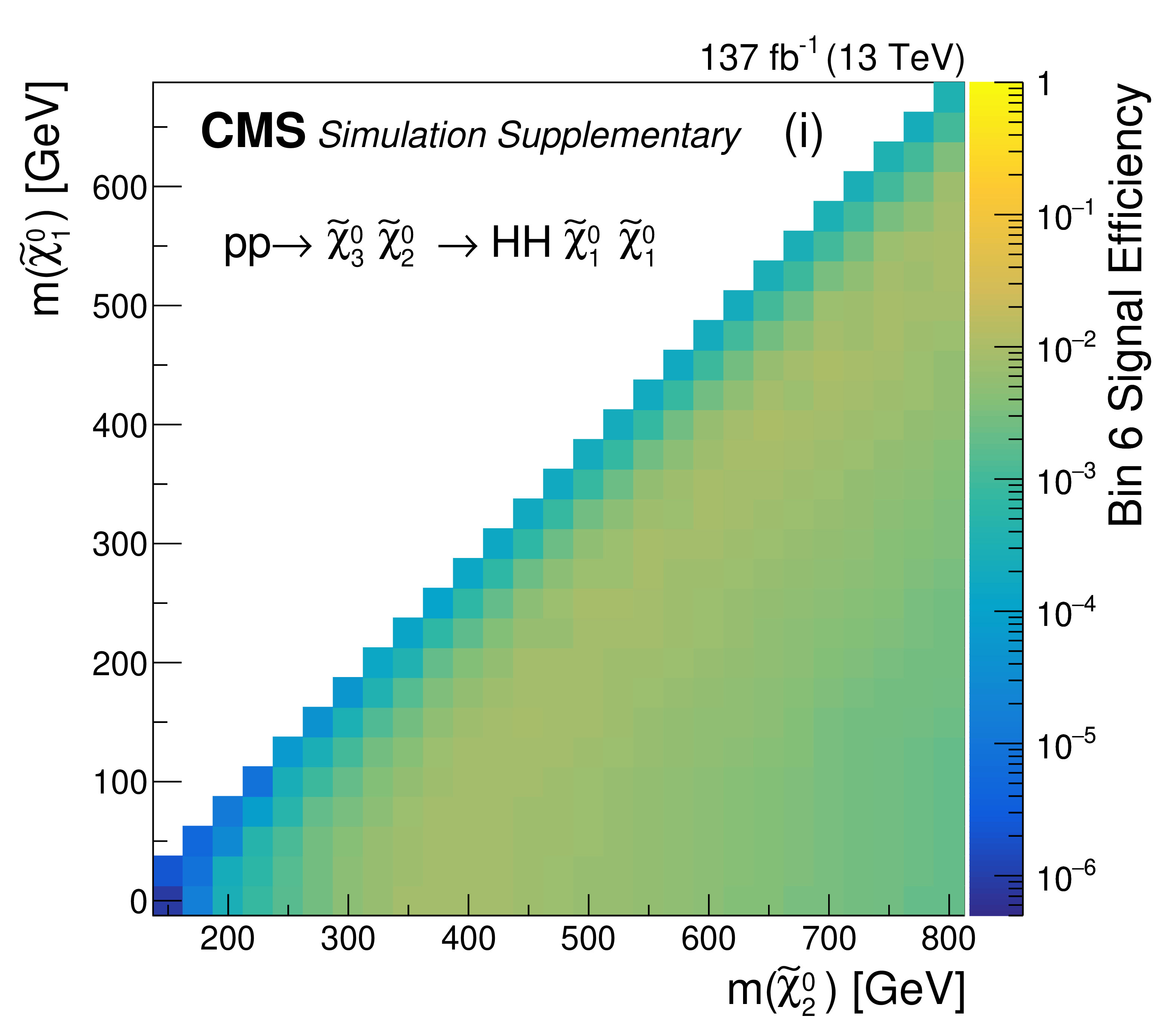
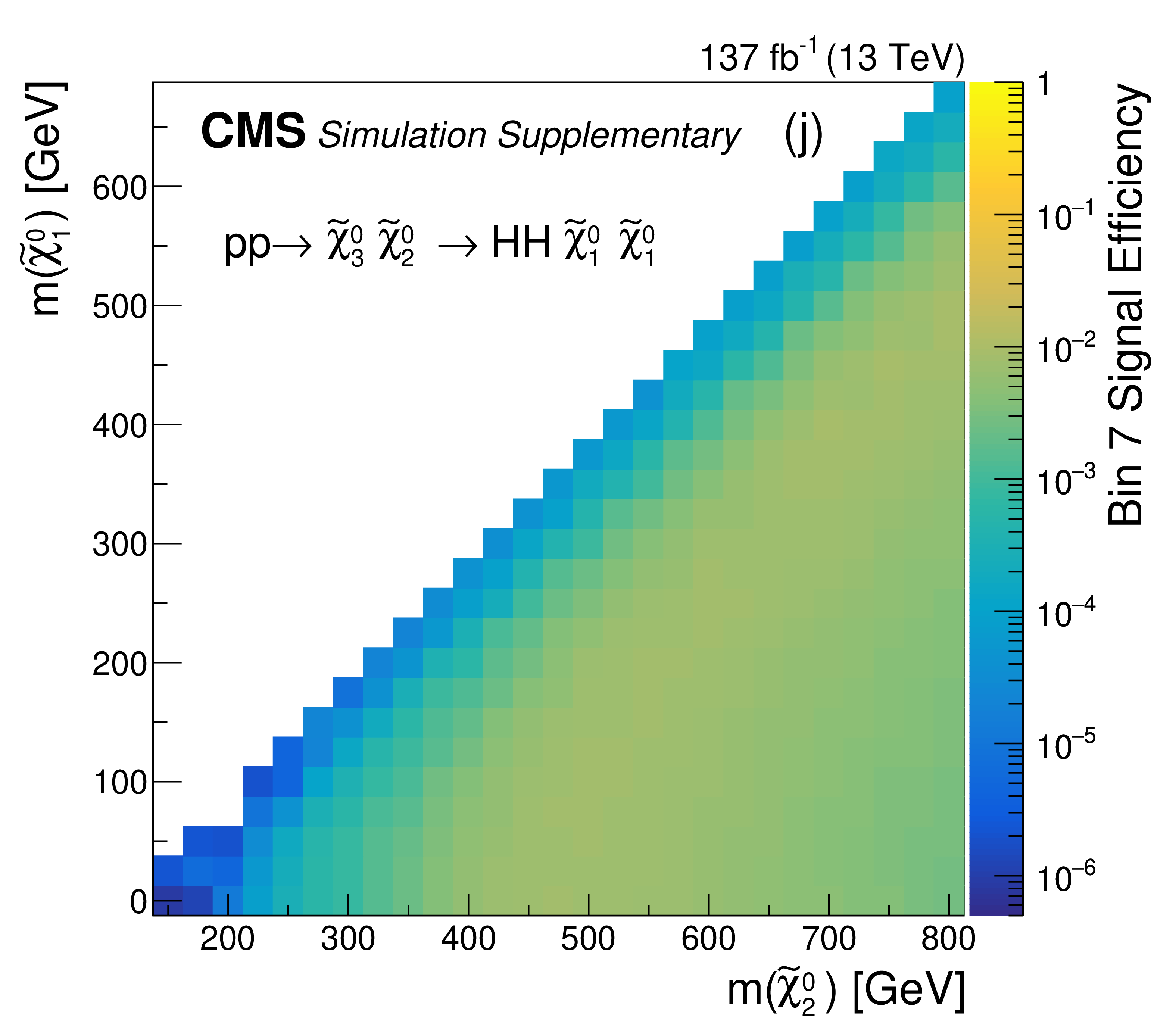
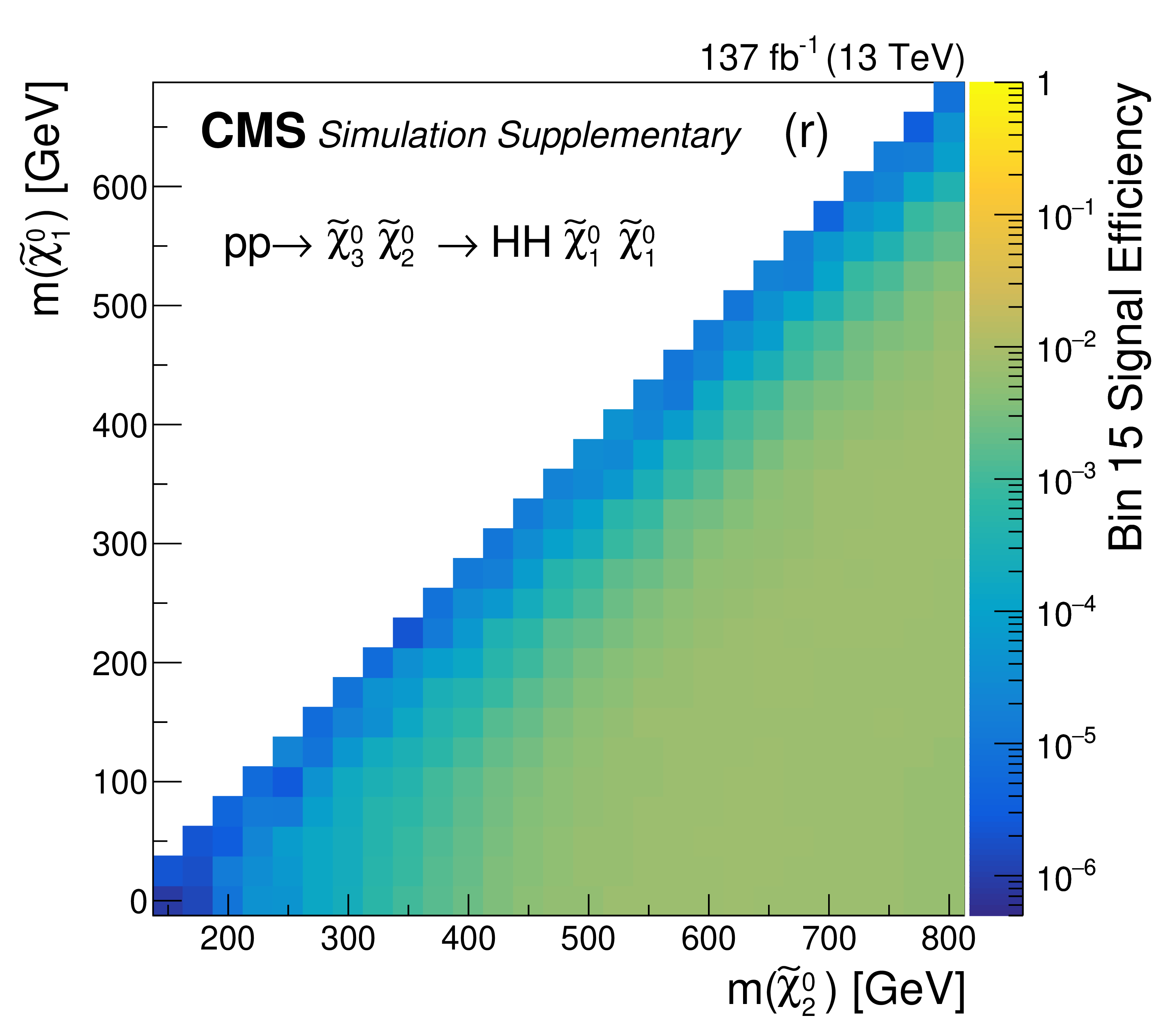
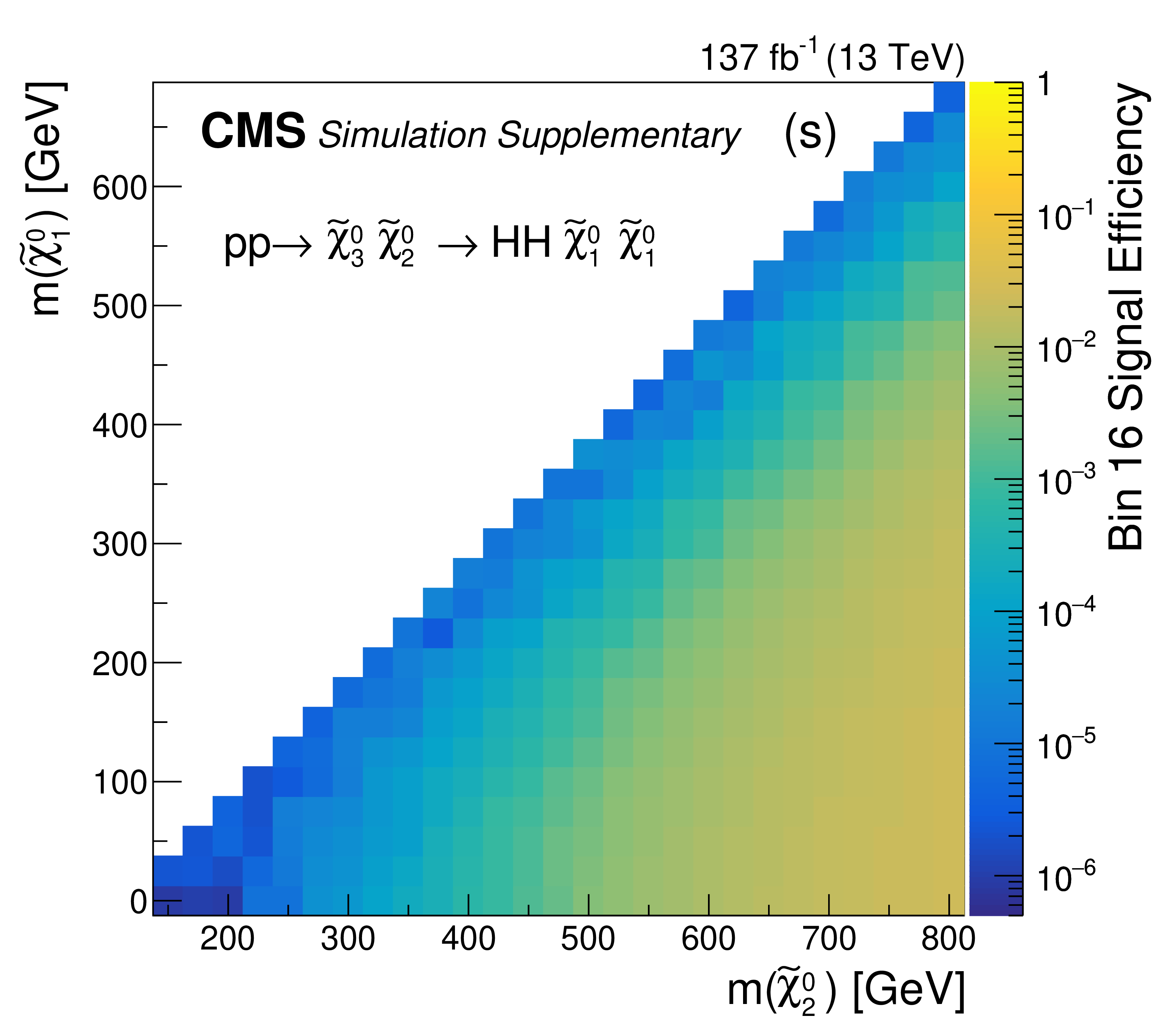
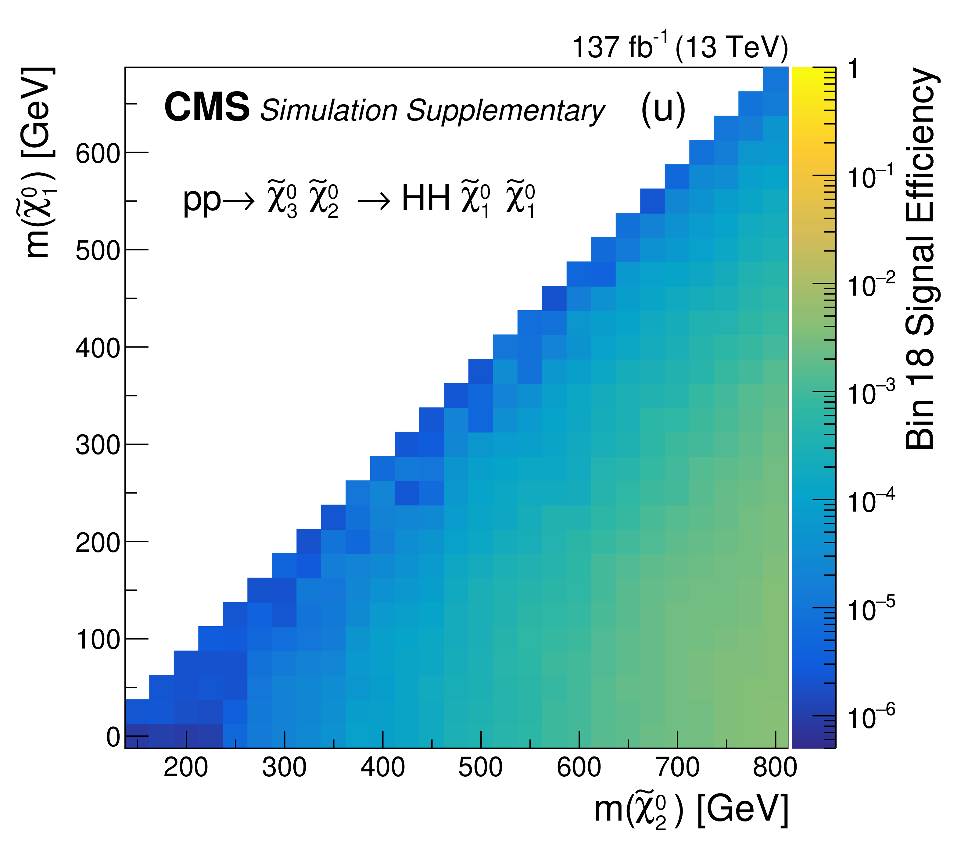
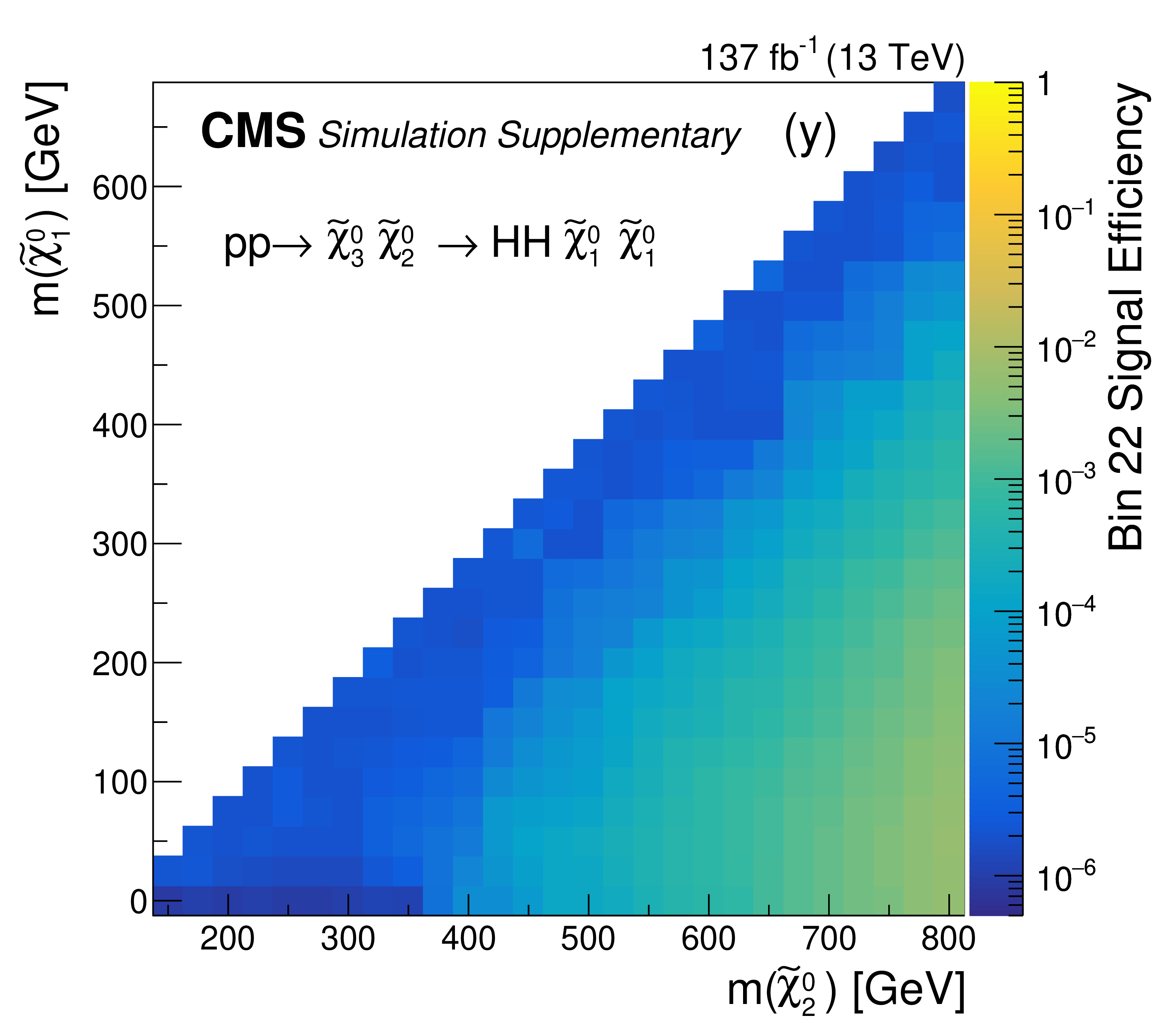
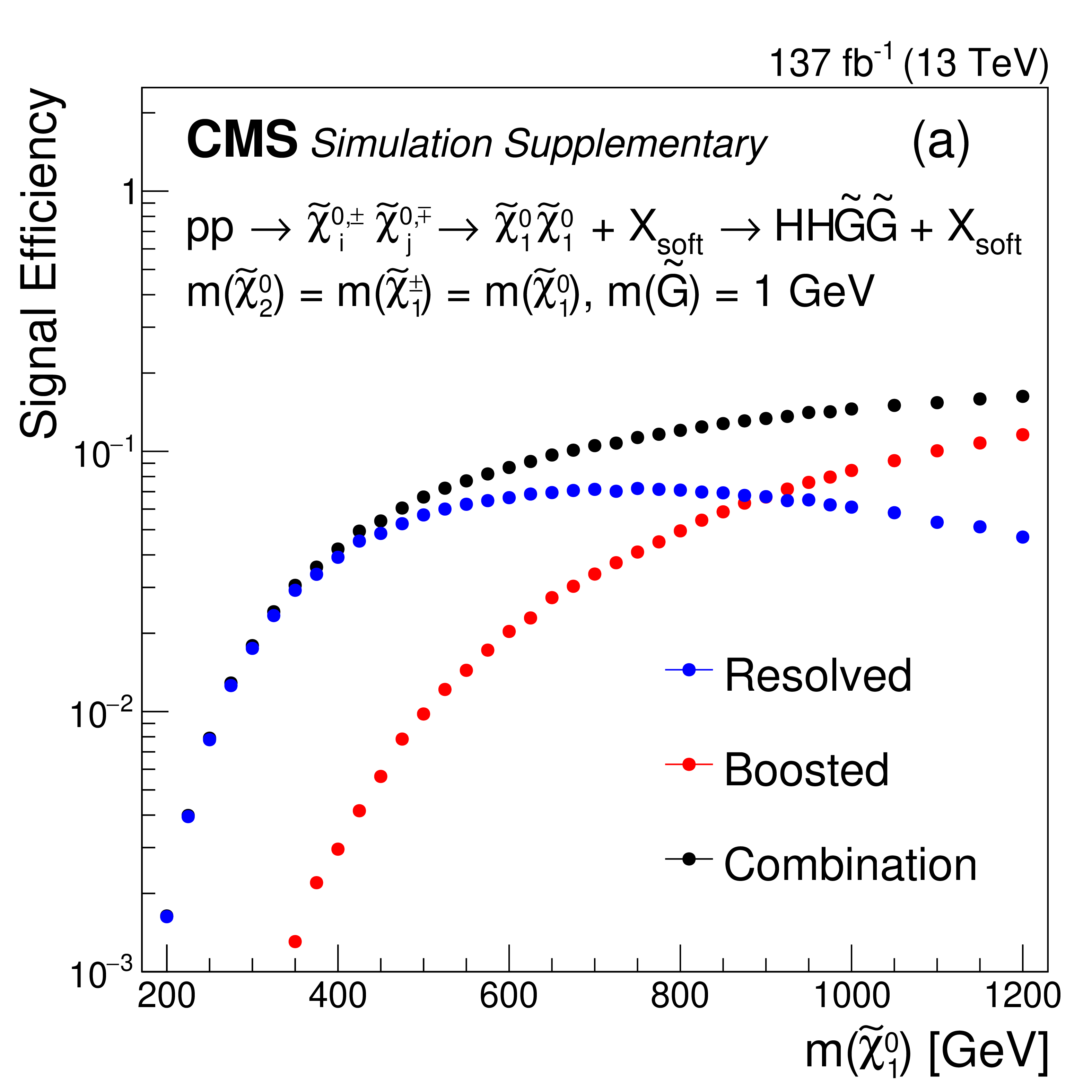
png pdf	Additional Figure 4: Efficiency for the TChiHH model, $\tilde{\chi}_2^0 \tilde{\chi}_2^0 \to \mathrm{H} \mathrm{H} \tilde{\chi}^0_1 \tilde{\chi}^0_1 $: (a) resolved SRs, (b) boosted SRs, (c) all SRs, and (d-y) SR 1-22. The SR indexing is given in Tables 4 and 5 of the paper. The denominator for the efficiency calculation includes only $\mathrm{H} \to \mathrm{b} \mathrm{\bar{b}} $ decays (for all SRs). Overlapping events between the two signatures have been removed from the boosted SRs.
png pdf root	Additional Figure 4-a: Efficiency for the TChiHH model, $\tilde{\chi}_2^0 \tilde{\chi}_2^0 \to \mathrm{H} \mathrm{H} \tilde{\chi}^0_1 \tilde{\chi}^0_1 $: resolved SRs. boosted SRs. The denominator for the efficiency calculation includes only $\mathrm{H} \to \mathrm{b} \mathrm{\bar{b}} $ decays.
png pdf root	Additional Figure 4-b: Efficiency for the TChiHH model, $\tilde{\chi}_2^0 \tilde{\chi}_2^0 \to \mathrm{H} \mathrm{H} \tilde{\chi}^0_1 \tilde{\chi}^0_1 $: boosted SRs. The denominator for the efficiency calculation includes only $\mathrm{H} \to \mathrm{b} \mathrm{\bar{b}} $ decays.
png pdf root	Additional Figure 4-c: Efficiency for the TChiHH model, $\tilde{\chi}_2^0 \tilde{\chi}_2^0 \to \mathrm{H} \mathrm{H} \tilde{\chi}^0_1 \tilde{\chi}^0_1 $: all SRs. The denominator for the efficiency calculation includes only $\mathrm{H} \to \mathrm{b} \mathrm{\bar{b}} $ decays.
png pdf root	Additional Figure 4-d: Efficiency for the TChiHH model, $\tilde{\chi}_2^0 \tilde{\chi}_2^0 \to \mathrm{H} \mathrm{H} \tilde{\chi}^0_1 \tilde{\chi}^0_1 $: SR 1. The denominator for the efficiency calculation includes only $\mathrm{H} \to \mathrm{b} \mathrm{\bar{b}} $ decays.
png pdf root	Additional Figure 4-e: Efficiency for the TChiHH model, $\tilde{\chi}_2^0 \tilde{\chi}_2^0 \to \mathrm{H} \mathrm{H} \tilde{\chi}^0_1 \tilde{\chi}^0_1 $: SR 2. The denominator for the efficiency calculation includes only $\mathrm{H} \to \mathrm{b} \mathrm{\bar{b}} $ decays.
png pdf root	Additional Figure 4-f: Efficiency for the TChiHH model, $\tilde{\chi}_2^0 \tilde{\chi}_2^0 \to \mathrm{H} \mathrm{H} \tilde{\chi}^0_1 \tilde{\chi}^0_1 $: SR 3. The denominator for the efficiency calculation includes only $\mathrm{H} \to \mathrm{b} \mathrm{\bar{b}} $ decays.
png pdf root	Additional Figure 4-g: Efficiency for the TChiHH model, $\tilde{\chi}_2^0 \tilde{\chi}_2^0 \to \mathrm{H} \mathrm{H} \tilde{\chi}^0_1 \tilde{\chi}^0_1 $: SR 4. The denominator for the efficiency calculation includes only $\mathrm{H} \to \mathrm{b} \mathrm{\bar{b}} $ decays.
png pdf root	Additional Figure 4-h: Efficiency for the TChiHH model, $\tilde{\chi}_2^0 \tilde{\chi}_2^0 \to \mathrm{H} \mathrm{H} \tilde{\chi}^0_1 \tilde{\chi}^0_1 $: SR 5. The denominator for the efficiency calculation includes only $\mathrm{H} \to \mathrm{b} \mathrm{\bar{b}} $ decays.
png pdf root	Additional Figure 4-i: Efficiency for the TChiHH model, $\tilde{\chi}_2^0 \tilde{\chi}_2^0 \to \mathrm{H} \mathrm{H} \tilde{\chi}^0_1 \tilde{\chi}^0_1 $: SR 6. The denominator for the efficiency calculation includes only $\mathrm{H} \to \mathrm{b} \mathrm{\bar{b}} $ decays.
png pdf root	Additional Figure 4-j: Efficiency for the TChiHH model, $\tilde{\chi}_2^0 \tilde{\chi}_2^0 \to \mathrm{H} \mathrm{H} \tilde{\chi}^0_1 \tilde{\chi}^0_1 $: SR 7. The denominator for the efficiency calculation includes only $\mathrm{H} \to \mathrm{b} \mathrm{\bar{b}} $ decays.
png pdf root	Additional Figure 4-k: Efficiency for the TChiHH model, $\tilde{\chi}_2^0 \tilde{\chi}_2^0 \to \mathrm{H} \mathrm{H} \tilde{\chi}^0_1 \tilde{\chi}^0_1 $: SR 8. The denominator for the efficiency calculation includes only $\mathrm{H} \to \mathrm{b} \mathrm{\bar{b}} $ decays.
png pdf root	Additional Figure 4-l: Efficiency for the TChiHH model, $\tilde{\chi}_2^0 \tilde{\chi}_2^0 \to \mathrm{H} \mathrm{H} \tilde{\chi}^0_1 \tilde{\chi}^0_1 $: SR 9. The denominator for the efficiency calculation includes only $\mathrm{H} \to \mathrm{b} \mathrm{\bar{b}} $ decays.
png pdf root	Additional Figure 4-m: Efficiency for the TChiHH model, $\tilde{\chi}_2^0 \tilde{\chi}_2^0 \to \mathrm{H} \mathrm{H} \tilde{\chi}^0_1 \tilde{\chi}^0_1 $: SR 10. The denominator for the efficiency calculation includes only $\mathrm{H} \to \mathrm{b} \mathrm{\bar{b}} $ decays.
png pdf root	Additional Figure 4-n: Efficiency for the TChiHH model, $\tilde{\chi}_2^0 \tilde{\chi}_2^0 \to \mathrm{H} \mathrm{H} \tilde{\chi}^0_1 \tilde{\chi}^0_1 $: SR 11. The denominator for the efficiency calculation includes only $\mathrm{H} \to \mathrm{b} \mathrm{\bar{b}} $ decays.
png pdf root	Additional Figure 4-o: Efficiency for the TChiHH model, $\tilde{\chi}_2^0 \tilde{\chi}_2^0 \to \mathrm{H} \mathrm{H} \tilde{\chi}^0_1 \tilde{\chi}^0_1 $: SR 12. The denominator for the efficiency calculation includes only $\mathrm{H} \to \mathrm{b} \mathrm{\bar{b}} $ decays.
png pdf root	Additional Figure 4-p: Efficiency for the TChiHH model, $\tilde{\chi}_2^0 \tilde{\chi}_2^0 \to \mathrm{H} \mathrm{H} \tilde{\chi}^0_1 \tilde{\chi}^0_1 $: SR 13. The denominator for the efficiency calculation includes only $\mathrm{H} \to \mathrm{b} \mathrm{\bar{b}} $ decays.
png pdf root	Additional Figure 4-q: Efficiency for the TChiHH model, $\tilde{\chi}_2^0 \tilde{\chi}_2^0 \to \mathrm{H} \mathrm{H} \tilde{\chi}^0_1 \tilde{\chi}^0_1 $: SR 14. The denominator for the efficiency calculation includes only $\mathrm{H} \to \mathrm{b} \mathrm{\bar{b}} $ decays.
png pdf root	Additional Figure 4-r: Efficiency for the TChiHH model, $\tilde{\chi}_2^0 \tilde{\chi}_2^0 \to \mathrm{H} \mathrm{H} \tilde{\chi}^0_1 \tilde{\chi}^0_1 $: SR 15. The denominator for the efficiency calculation includes only $\mathrm{H} \to \mathrm{b} \mathrm{\bar{b}} $ decays.
png pdf root	Additional Figure 4-s: Efficiency for the TChiHH model, $\tilde{\chi}_2^0 \tilde{\chi}_2^0 \to \mathrm{H} \mathrm{H} \tilde{\chi}^0_1 \tilde{\chi}^0_1 $: SR 16. The denominator for the efficiency calculation includes only $\mathrm{H} \to \mathrm{b} \mathrm{\bar{b}} $ decays.
png pdf root	Additional Figure 4-t: Efficiency for the TChiHH model, $\tilde{\chi}_2^0 \tilde{\chi}_2^0 \to \mathrm{H} \mathrm{H} \tilde{\chi}^0_1 \tilde{\chi}^0_1 $: SR 17. The denominator for the efficiency calculation includes only $\mathrm{H} \to \mathrm{b} \mathrm{\bar{b}} $ decays.
png pdf root	Additional Figure 4-u: Efficiency for the TChiHH model, $\tilde{\chi}_2^0 \tilde{\chi}_2^0 \to \mathrm{H} \mathrm{H} \tilde{\chi}^0_1 \tilde{\chi}^0_1 $: SR 18. The denominator for the efficiency calculation includes only $\mathrm{H} \to \mathrm{b} \mathrm{\bar{b}} $ decays.
png pdf root	Additional Figure 4-v: Efficiency for the TChiHH model, $\tilde{\chi}_2^0 \tilde{\chi}_2^0 \to \mathrm{H} \mathrm{H} \tilde{\chi}^0_1 \tilde{\chi}^0_1 $: SR 19. The denominator for the efficiency calculation includes only $\mathrm{H} \to \mathrm{b} \mathrm{\bar{b}} $ decays.
png pdf root	Additional Figure 4-w: Efficiency for the TChiHH model, $\tilde{\chi}_2^0 \tilde{\chi}_2^0 \to \mathrm{H} \mathrm{H} \tilde{\chi}^0_1 \tilde{\chi}^0_1 $: SR 20. The denominator for the efficiency calculation includes only $\mathrm{H} \to \mathrm{b} \mathrm{\bar{b}} $ decays.
png pdf root	Additional Figure 4-x: Efficiency for the TChiHH model, $\tilde{\chi}_2^0 \tilde{\chi}_2^0 \to \mathrm{H} \mathrm{H} \tilde{\chi}^0_1 \tilde{\chi}^0_1 $: SR 21. The denominator for the efficiency calculation includes only $\mathrm{H} \to \mathrm{b} \mathrm{\bar{b}} $ decays.
png pdf root	Additional Figure 4-y: Efficiency for the TChiHH model, $\tilde{\chi}_2^0 \tilde{\chi}_2^0 \to \mathrm{H} \mathrm{H} \tilde{\chi}^0_1 \tilde{\chi}^0_1 $: SR 22. The denominator for the efficiency calculation includes only $\mathrm{H} \to \mathrm{b} \mathrm{\bar{b}} $ decays.
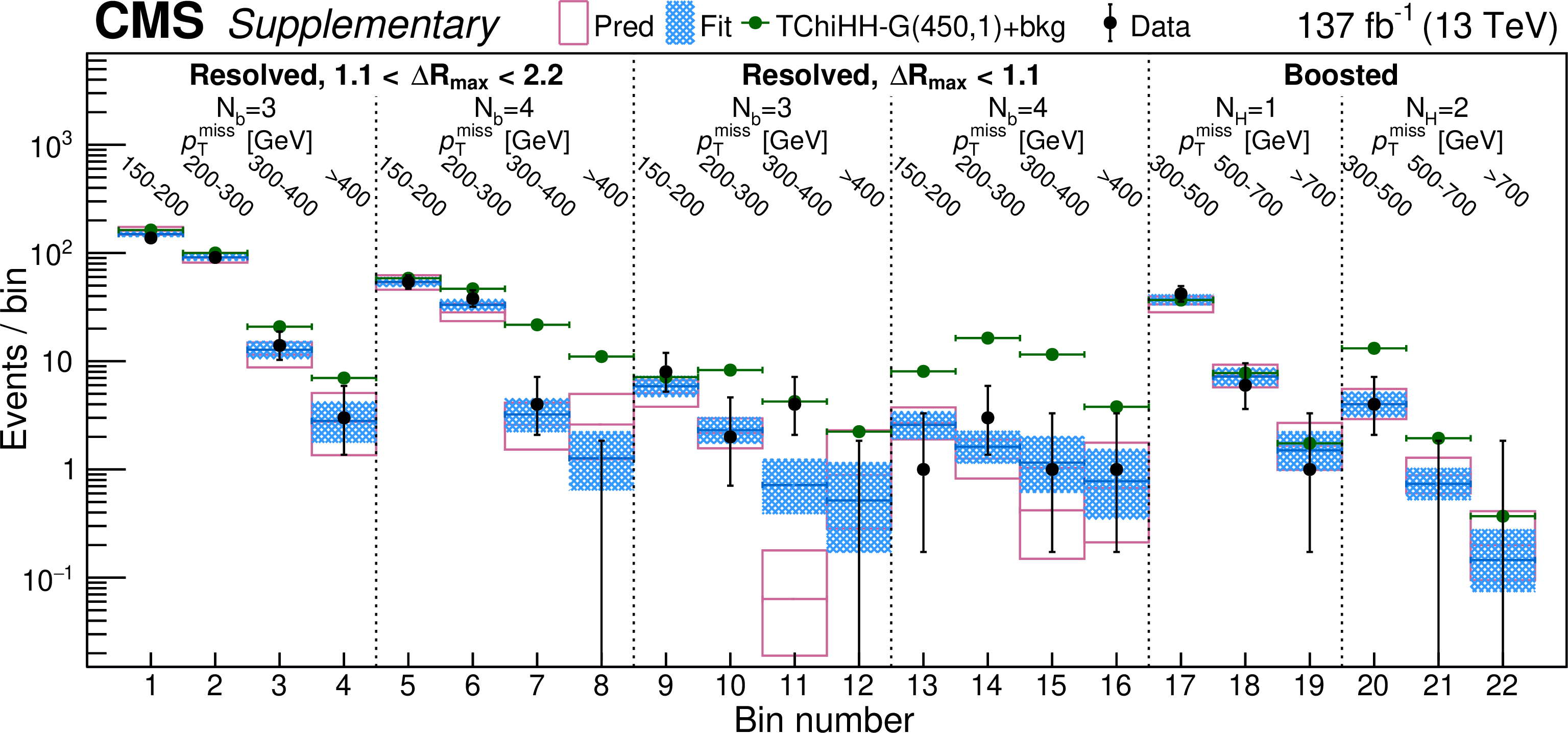
png pdf	Additional Figure 5: Observed and predicted yields in the search regions identified by the legend text. The black points with vertical error bars represent the observed yields, the magenta outline bands the background yields derived from the data sidebands with their total uncertainty, blue shaded bands the values determined by the background-only fit, and the green points with horizontal bars (indicating the bin width) the sum of the background yields derived from the data sidebands and the yields of the TChiHH-G(450,1) model with signal strength 1.
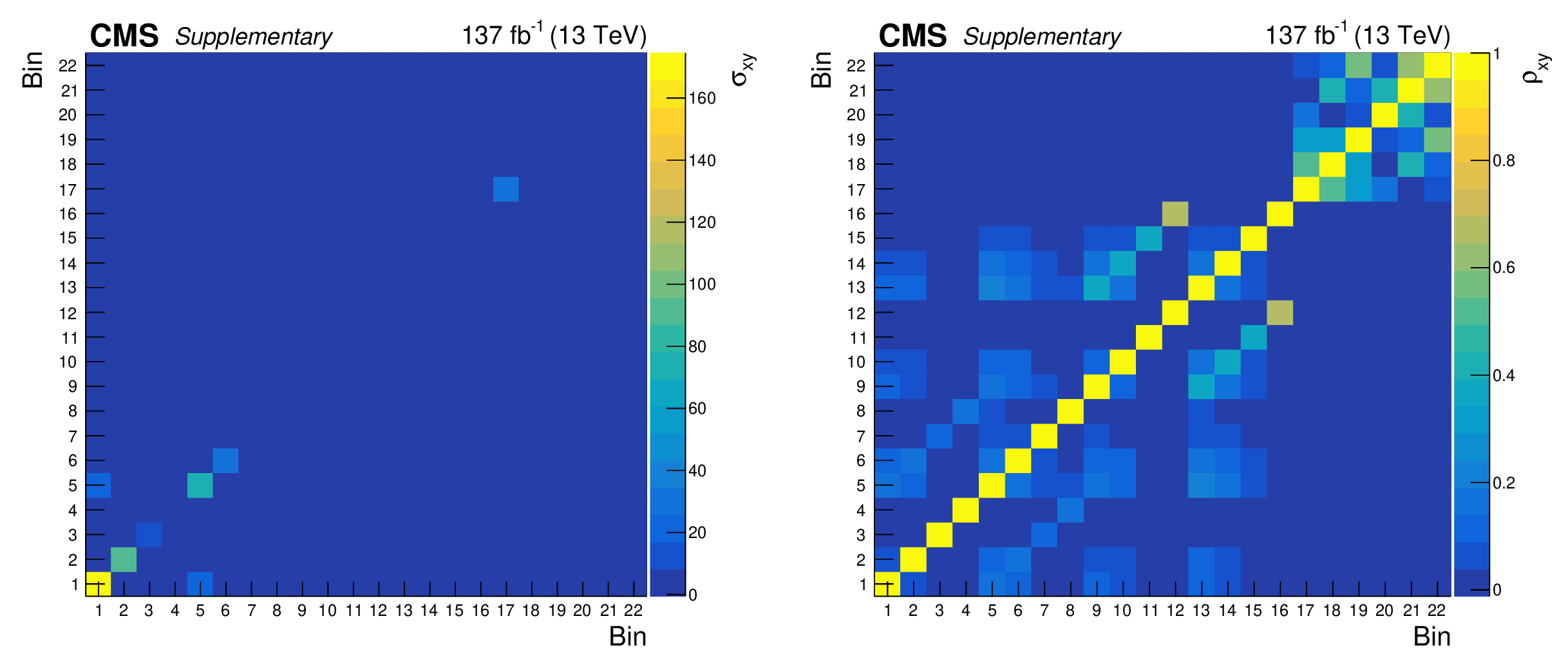
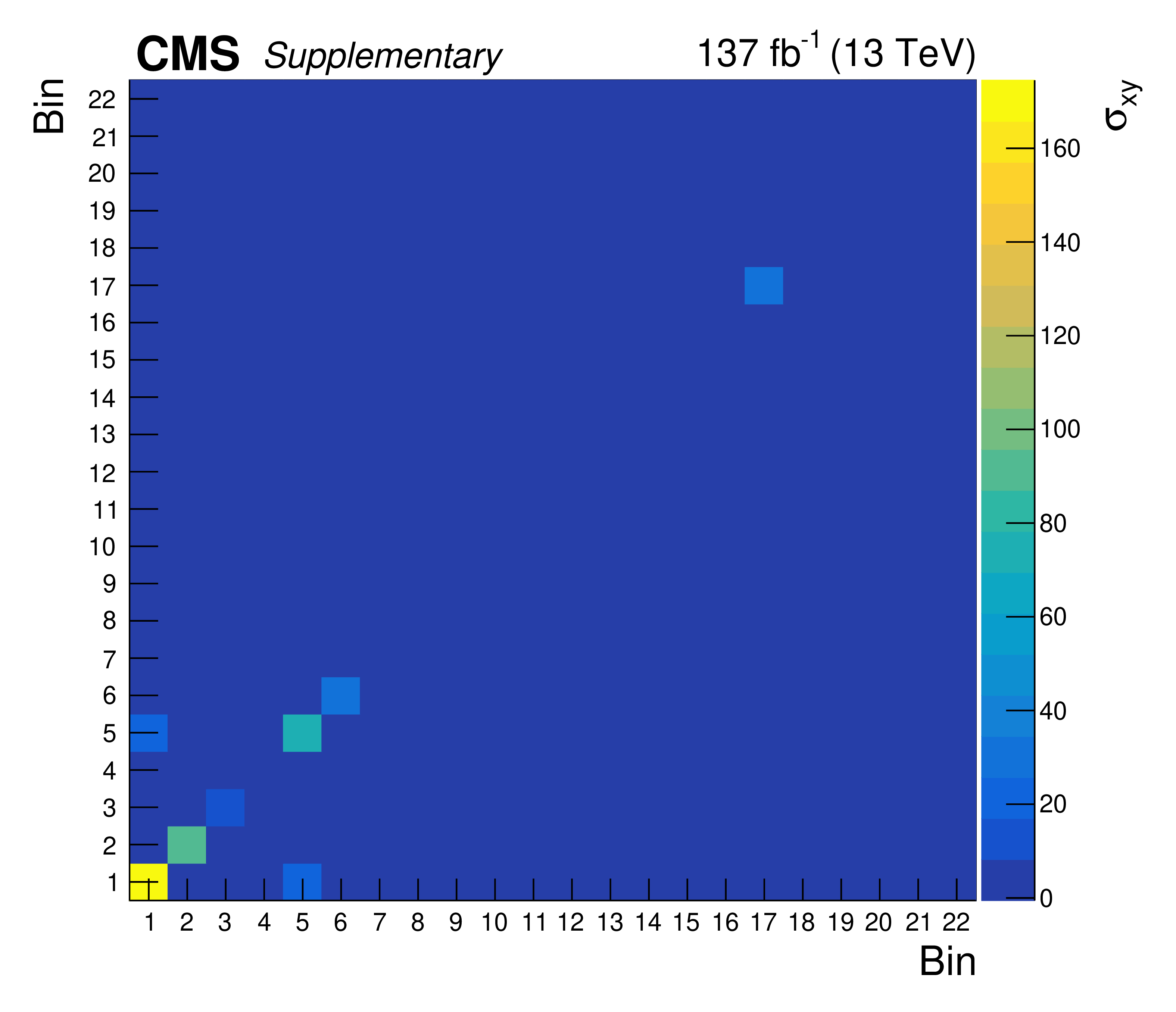
png pdf	Additional Figure 6: (a) Covariance and (b) correlation matrices for the 22 search bins, ordered as in Tables 4 and 5 of the paper.
png pdf root	Additional Figure 6-a: Covariance matrix for the 22 search bins, ordered as in Tables 4 and 5 of the paper.
png pdf root	Additional Figure 6-b: Correlation matrix for the 22 search bins, ordered as in Tables 4 and 5 of the paper.
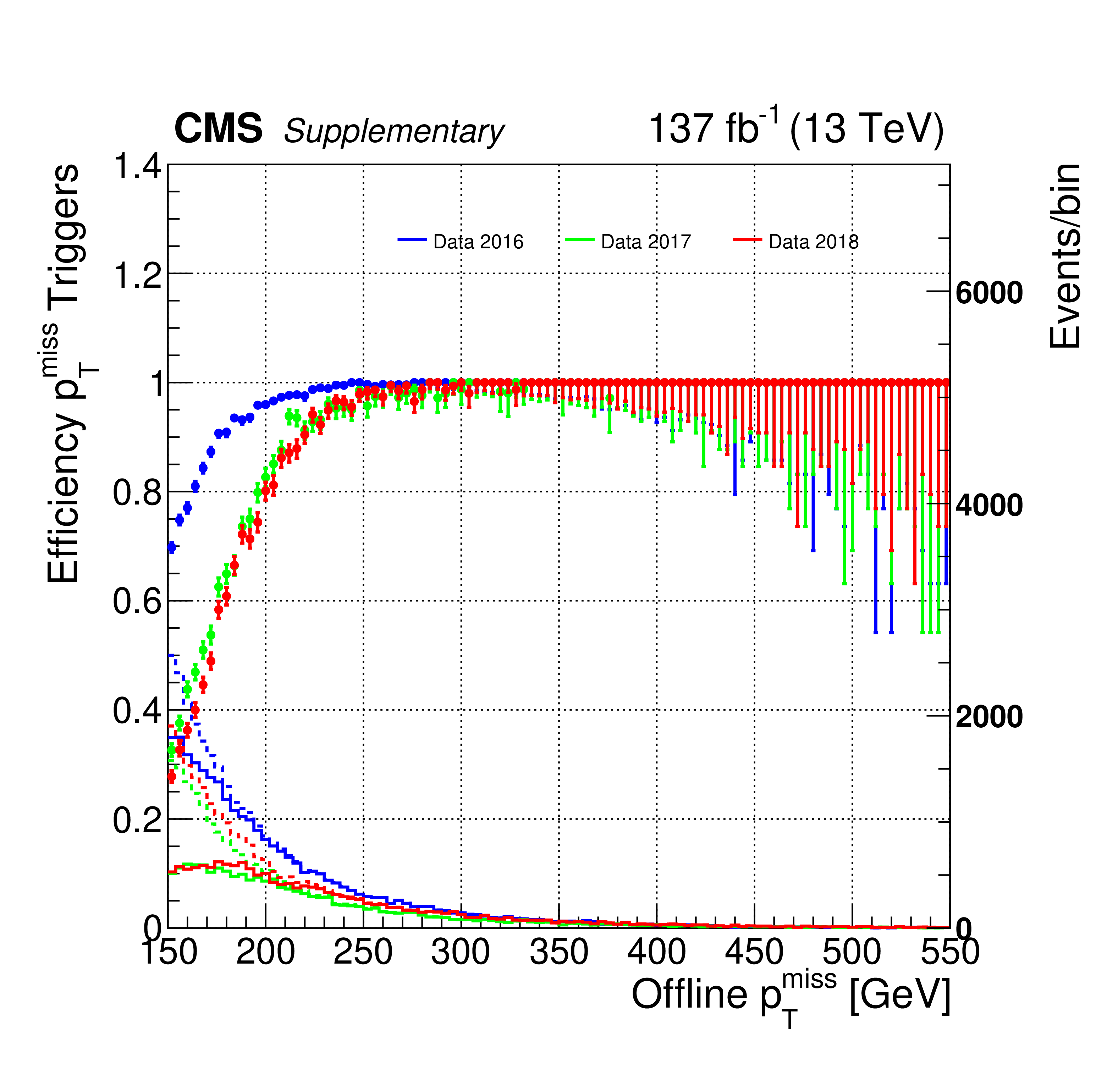
png pdf	Additional Figure 7: ${{p_{\mathrm {T}}} ^\text {miss}}$ trigger efficiency (points) as a function of ${{p_{\mathrm {T}}} ^\text {miss}}$ for each year of data taking. The trigger threshold varied between 90 and 140 GeV, depending on the LHC instantaneous luminosity resulting in different efficiencies for each year. For large values of ${{p_{\mathrm {T}}} ^\text {miss}}$, the efficiency for all three years is unity. The solid (dashed) histogram gives the corresponding event count for the numerator (denominator) entering into the efficiency calculation.
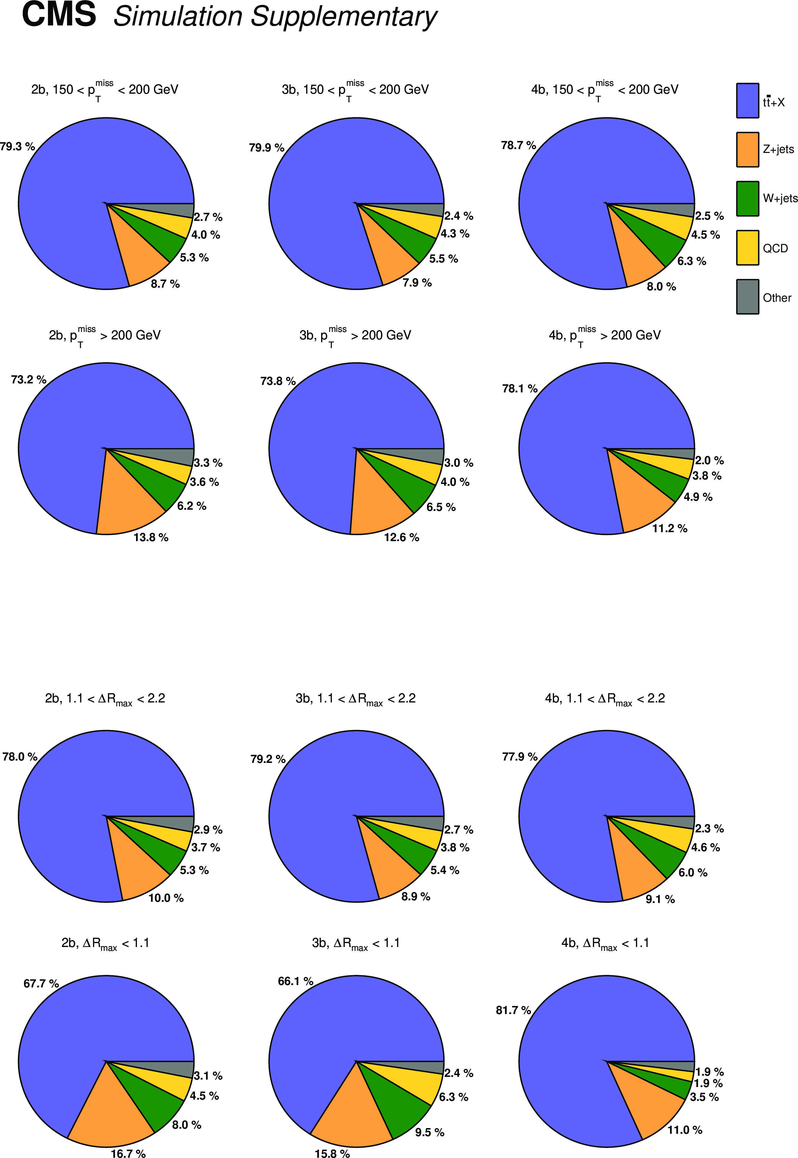
png pdf	Additional Figure 8: The background composition for different categories for the resolved topology. The columns correspond to 2b (left), 3b (center), and 4b (right). Each row has one selection in addition to the baseline selection, 150 $ < {{p_{\mathrm {T}}} ^\text {miss}} < $ 200 GeV (top row), $ {{p_{\mathrm {T}}} ^\text {miss}} > $ 200 GeV (second row), 1.1 $ < \Delta R_{\text {max}} < $ 2.2 (third row), and $\Delta R_{\text {max}} < $ 1.1 (bottom row).
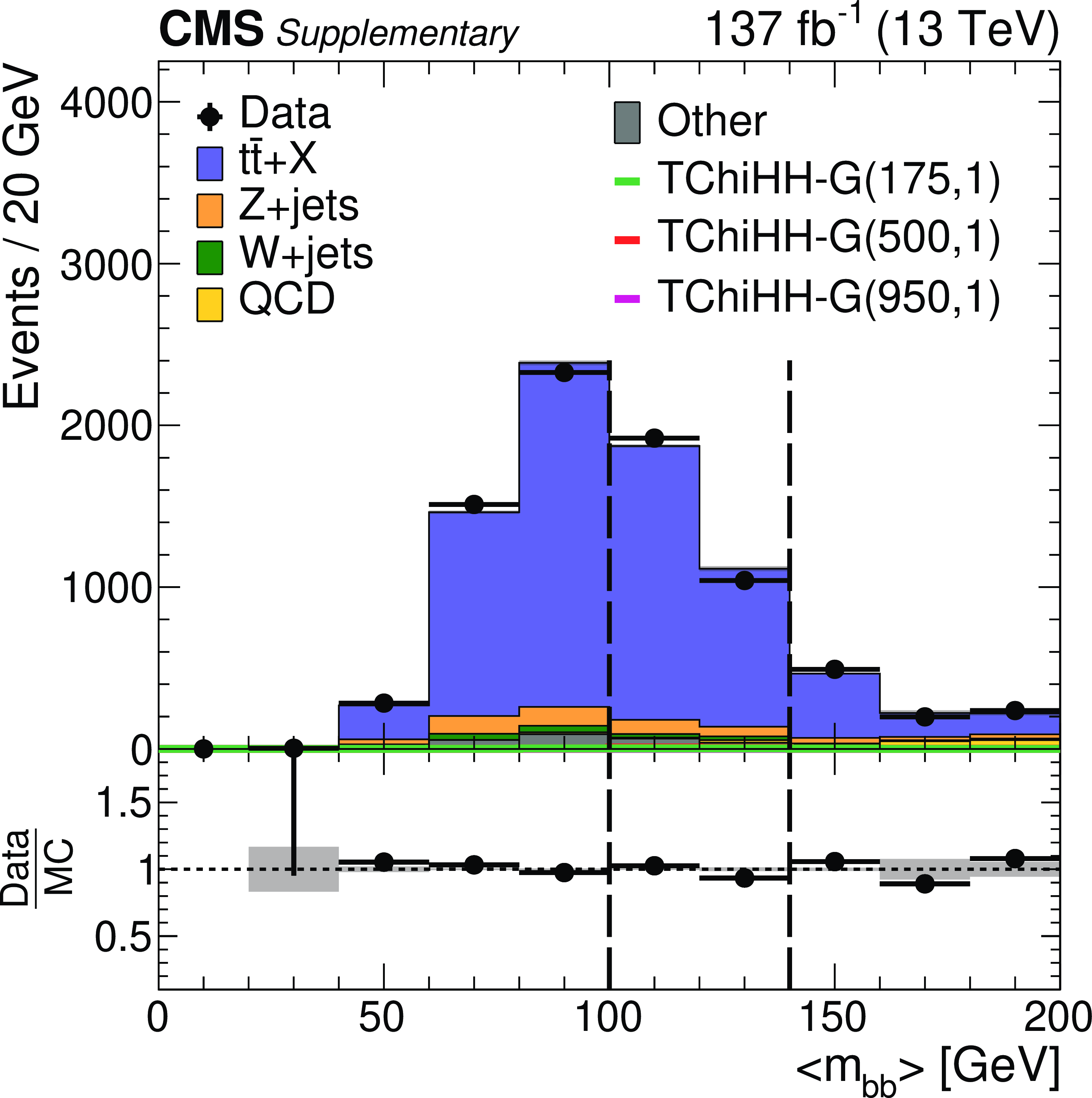
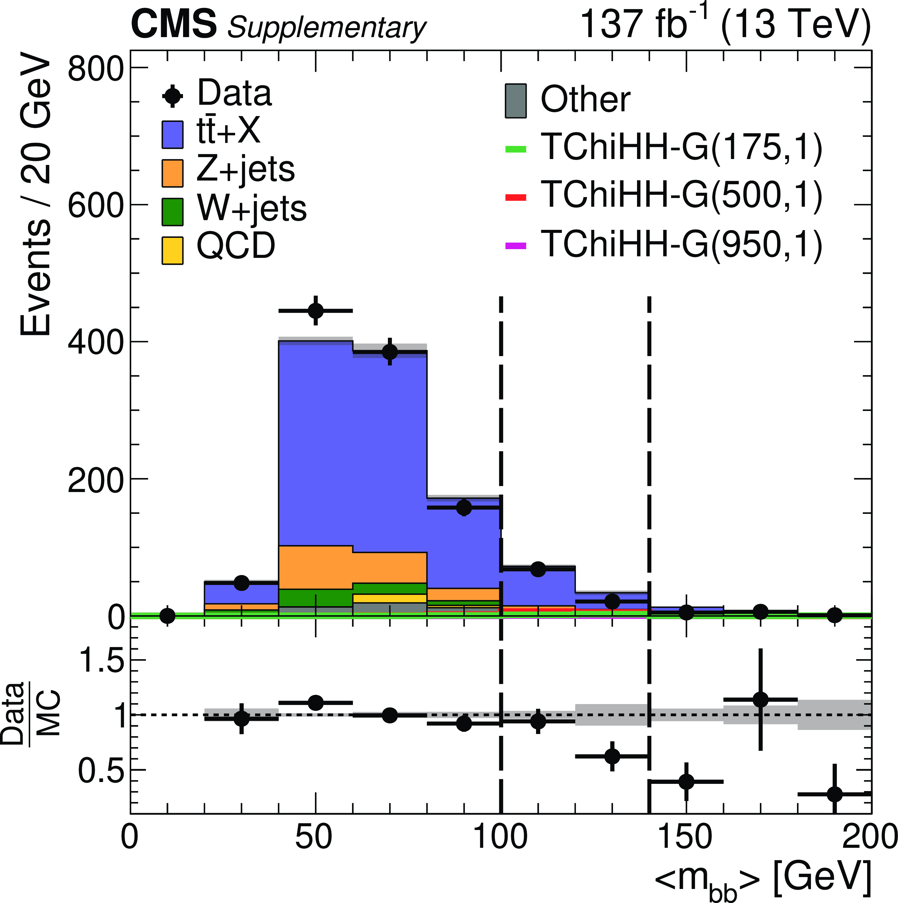
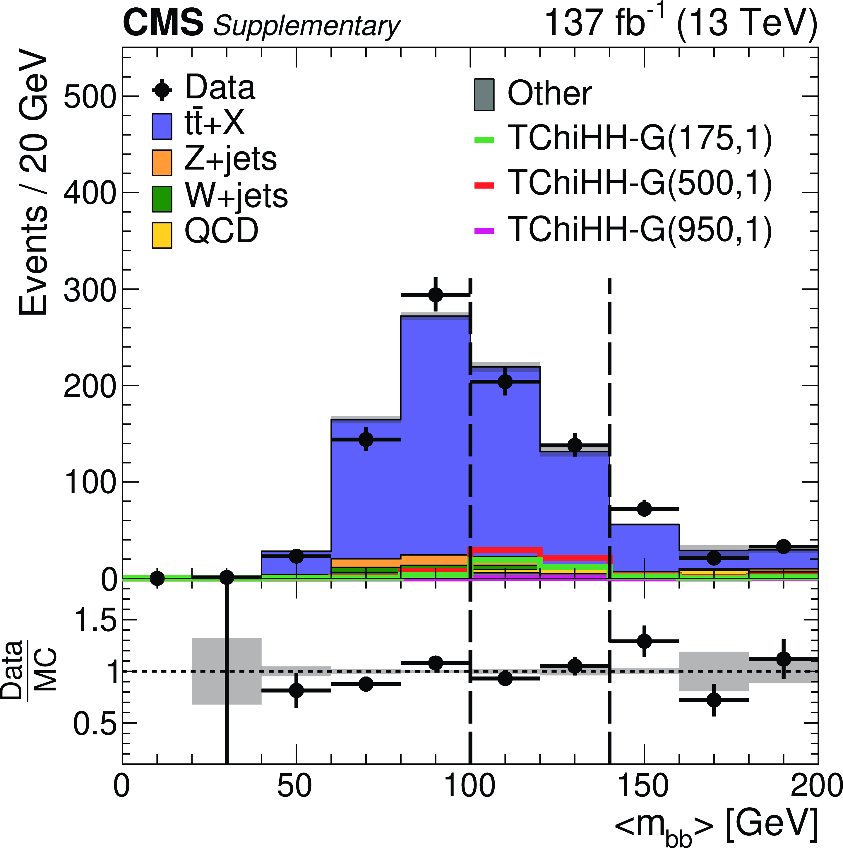
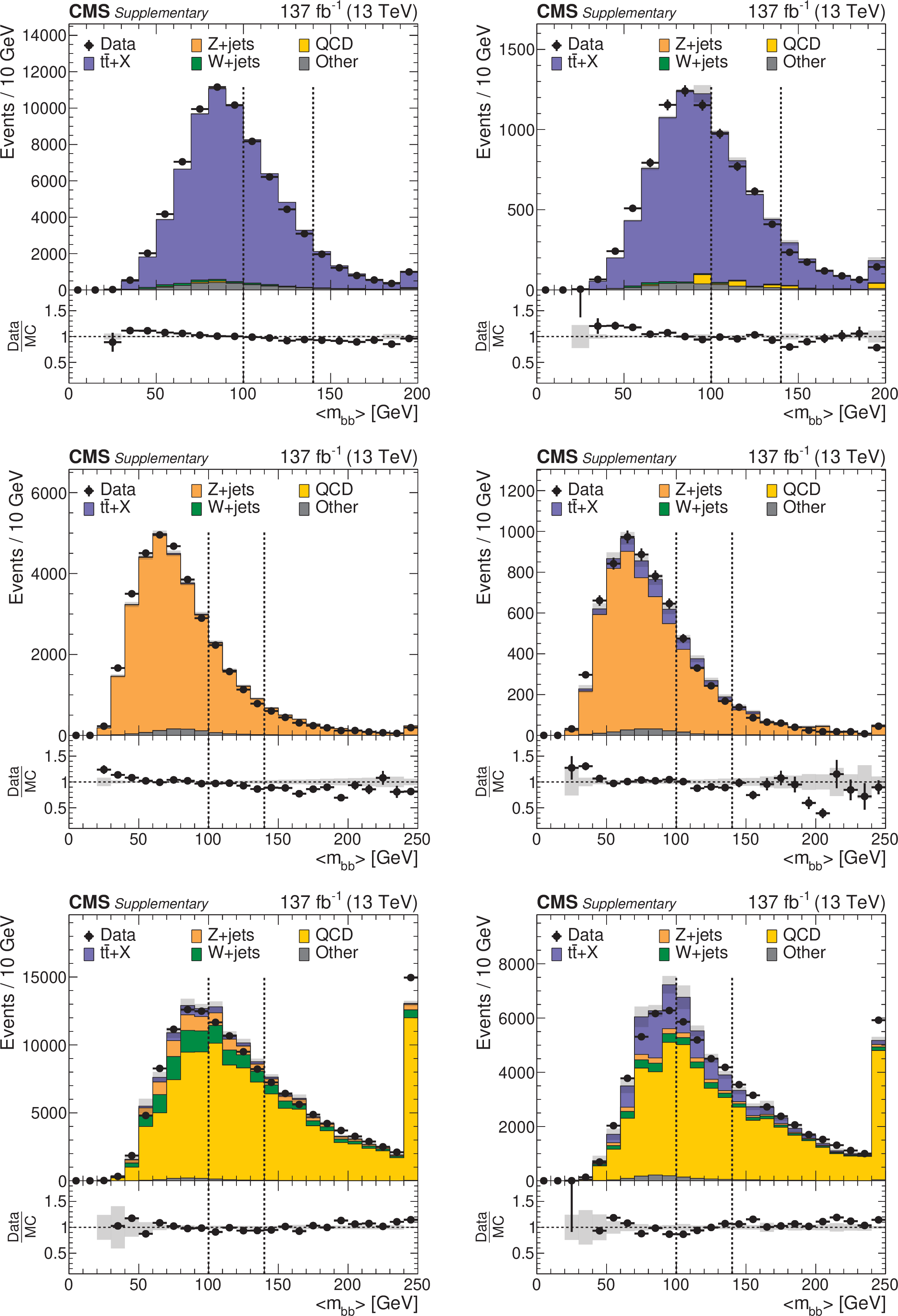
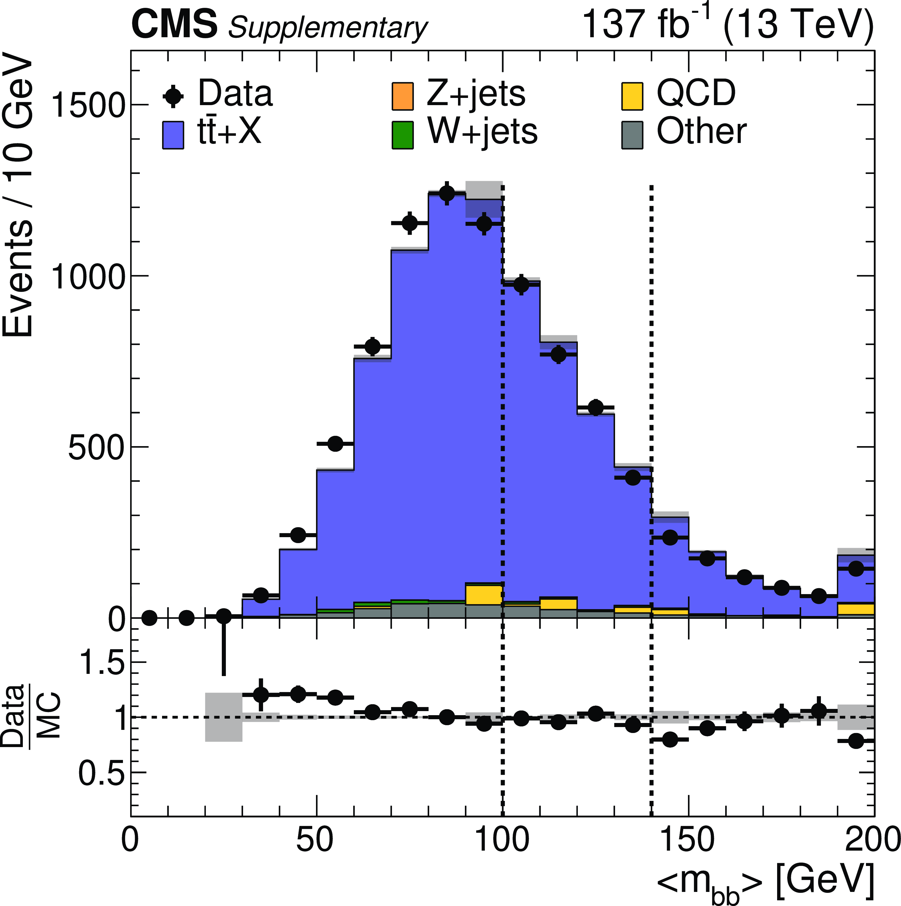
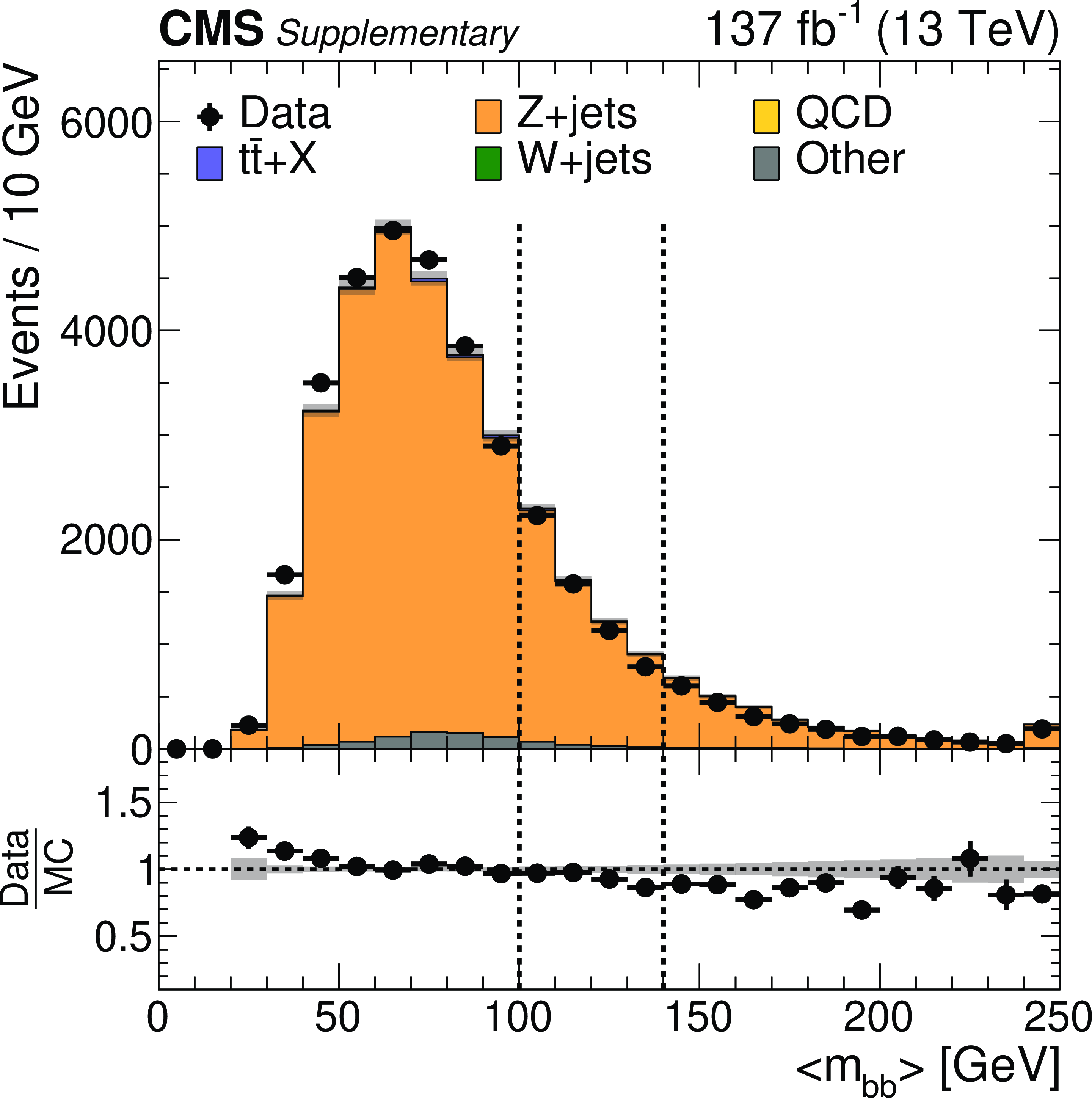
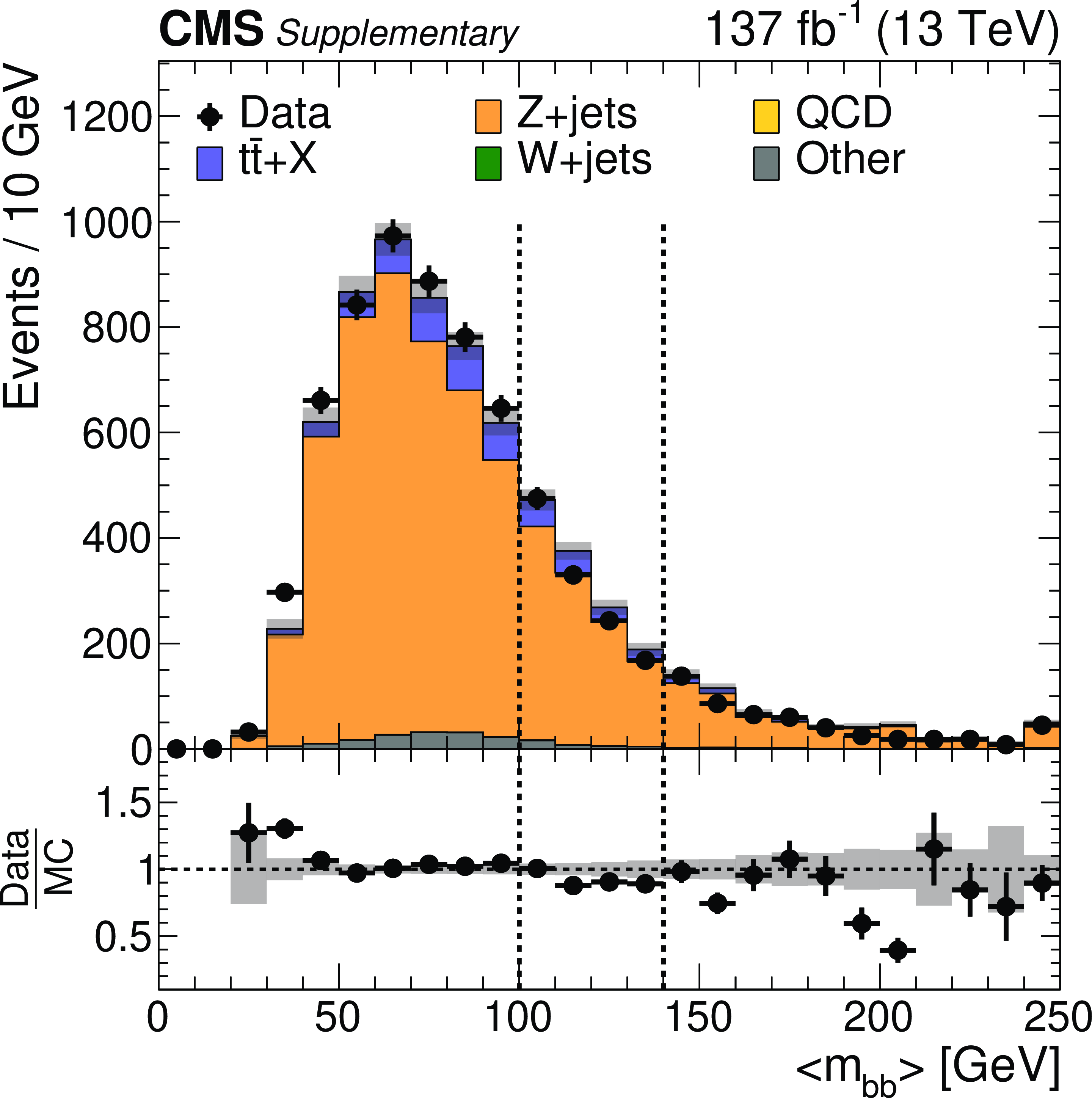
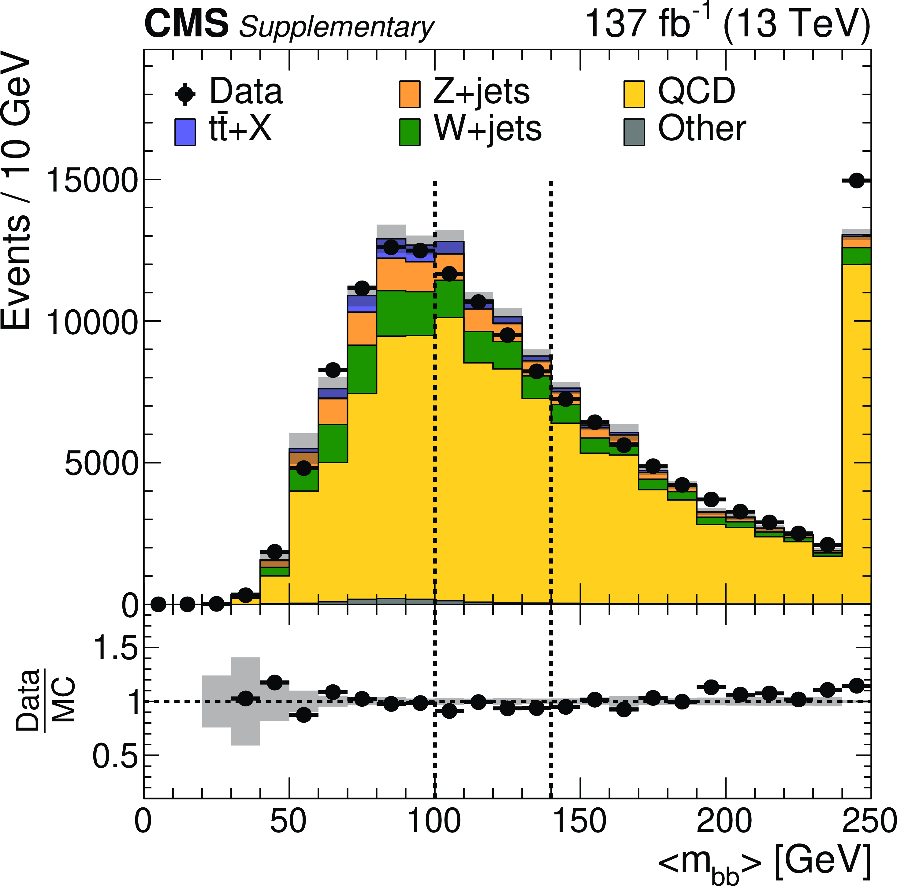
png pdf	Additional Figure 9: Distributions of $< m_{\mathrm{b} \mathrm{b}}> $ for data and simulation in various categories within the resolved signature baseline selection: (a) 2b and 1.1 $ < \Delta R_{\text {max}} < $ 2.2, (b) 2b and $\Delta R_{\text {max}} < $ 1.1, (c) 3-4b and 1.1 $ < \Delta R_{\text {max}} < $ 2.2, (d) 3-4b and $\Delta R_{\text {max}} < $ 1.1, (e) 2b and 150 $ < {{p_{\mathrm {T}}} ^\text {miss}} < $ 200 GeV, (f) 2b and $ {{p_{\mathrm {T}}} ^\text {miss}} > $ 200 GeV, (g) 3 and 4b $-$150 $ < {{p_{\mathrm {T}}} ^\text {miss}} < $ 200 GeV, and (h) 3-4b and $ {{p_{\mathrm {T}}} ^\text {miss}} > $ 200 GeV.
png pdf	Additional Figure 9-a: Distribution of $< m_{\mathrm{b} \mathrm{b}}> $ for data and simulation in the 2b and 1.1 $ < \Delta R_{\text {max}} < $ 2.2 category.
png pdf	Additional Figure 9-b: Distribution of $< m_{\mathrm{b} \mathrm{b}}> $ for data and simulation in the 2b and $\Delta R_{\text {max}} < $ 1.1 category.
png pdf	Additional Figure 9-c: Distribution of $< m_{\mathrm{b} \mathrm{b}}> $ for data and simulation in the 3-4b and 1.1 $ < \Delta R_{\text {max}} < $ 2.2 category.
png pdf	Additional Figure 9-d: Distribution of $< m_{\mathrm{b} \mathrm{b}}> $ for data and simulation in the 3-4b and $\Delta R_{\text {max}} < $ 1.1 category.
png pdf	Additional Figure 9-e: Distribution of $< m_{\mathrm{b} \mathrm{b}}> $ for data and simulation in the 2b and 150 $ < {{p_{\mathrm {T}}} ^\text {miss}} < $ 200 GeV category.
png pdf	Additional Figure 9-f: Distribution of $< m_{\mathrm{b} \mathrm{b}}> $ for data and simulation in the 2b and $ {{p_{\mathrm {T}}} ^\text {miss}} > $ 200 GeV category.
png pdf	Additional Figure 9-g: Distribution of $< m_{\mathrm{b} \mathrm{b}}> $ for data and simulation in the 3 and 4b $-$150 $ < {{p_{\mathrm {T}}} ^\text {miss}} < $ 200 GeV category.
png pdf	Additional Figure 9-h: Distribution of $< m_{\mathrm{b} \mathrm{b}}> $ for data and simulation in the 3-4b and $ {{p_{\mathrm {T}}} ^\text {miss}} > $ 200 GeV category.
png pdf	Additional Figure 10: Distributions in $< m_{\mathrm{b} \mathrm{b}}> $ for data and simulated control samples of the resolved signature: (a, b) the 1-lepton control sample with $ {{p_{\mathrm {T}}} ^\text {miss}} > $ 75 GeV for the 2b and 3-4b categories respectively; (c, d) the 2-lepton control sample for the 0b and 1b categories respectively; and (e, f) the low-$\Delta \phi $ control sample for the 0b and 1b categories respectively.
png pdf	Additional Figure 10-a: Distributions in $< m_{\mathrm{b} \mathrm{b}}> $ for data and simulated control samples of the resolved signature: the 1-lepton control sample with $ {{p_{\mathrm {T}}} ^\text {miss}} > $ 75 GeV for the 2b category.
png pdf	Additional Figure 10-b: Distributions in $< m_{\mathrm{b} \mathrm{b}}> $ for data and simulated control samples of the resolved signature:
png pdf	Additional Figure 10-c: Distributions in $< m_{\mathrm{b} \mathrm{b}}> $ for data and simulated control samples of the resolved signature: the 2-lepton control sample for the 0b category.
png pdf	Additional Figure 10-d: Distributions in $< m_{\mathrm{b} \mathrm{b}}> $ for data and simulated control samples of the resolved signature: the 2-lepton control sample for the 1b category.
png pdf	Additional Figure 10-e: Distributions in $< m_{\mathrm{b} \mathrm{b}}> $ for data and simulated control samples of the resolved signature: the low-$\Delta \phi $ control sample for the 0b category.
png pdf	Additional Figure 10-f: Distributions in $< m_{\mathrm{b} \mathrm{b}}> $ for data and simulated control samples of the resolved signature: the low-$\Delta \phi $ control sample for the 1b category.
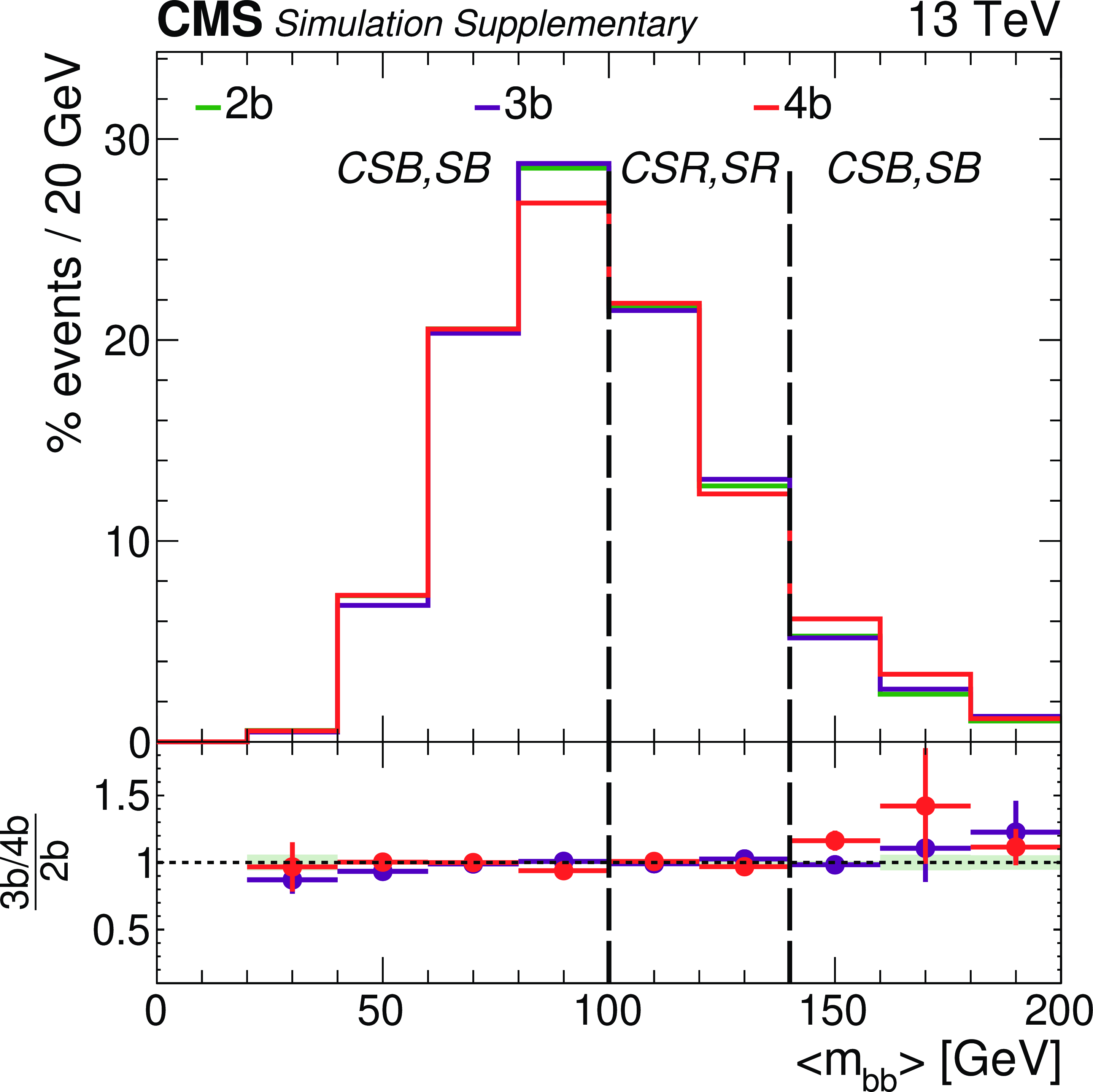
png pdf	Additional Figure 11: Comparison of the $< m_{\mathrm{b} \mathrm{b}}> $ shape among the $N_{\mathrm{b}}=$ 2, 3, and 4 regions for the background simulation. The histograms are normalized to a common area. The regions CSR and SR are defined to be within the H mass window 100 $ < \, < m_{\mathrm{b} \mathrm{b}}> \, < $ 140 GeV, and CSB and SB are outside of the H mass window, 0 $ < < m_{\mathrm{b} \mathrm{b}}> < $ 100 GeV or 140 $ < \, < m_{\mathrm{b} \mathrm{b}}> \, < $ 200 GeV.
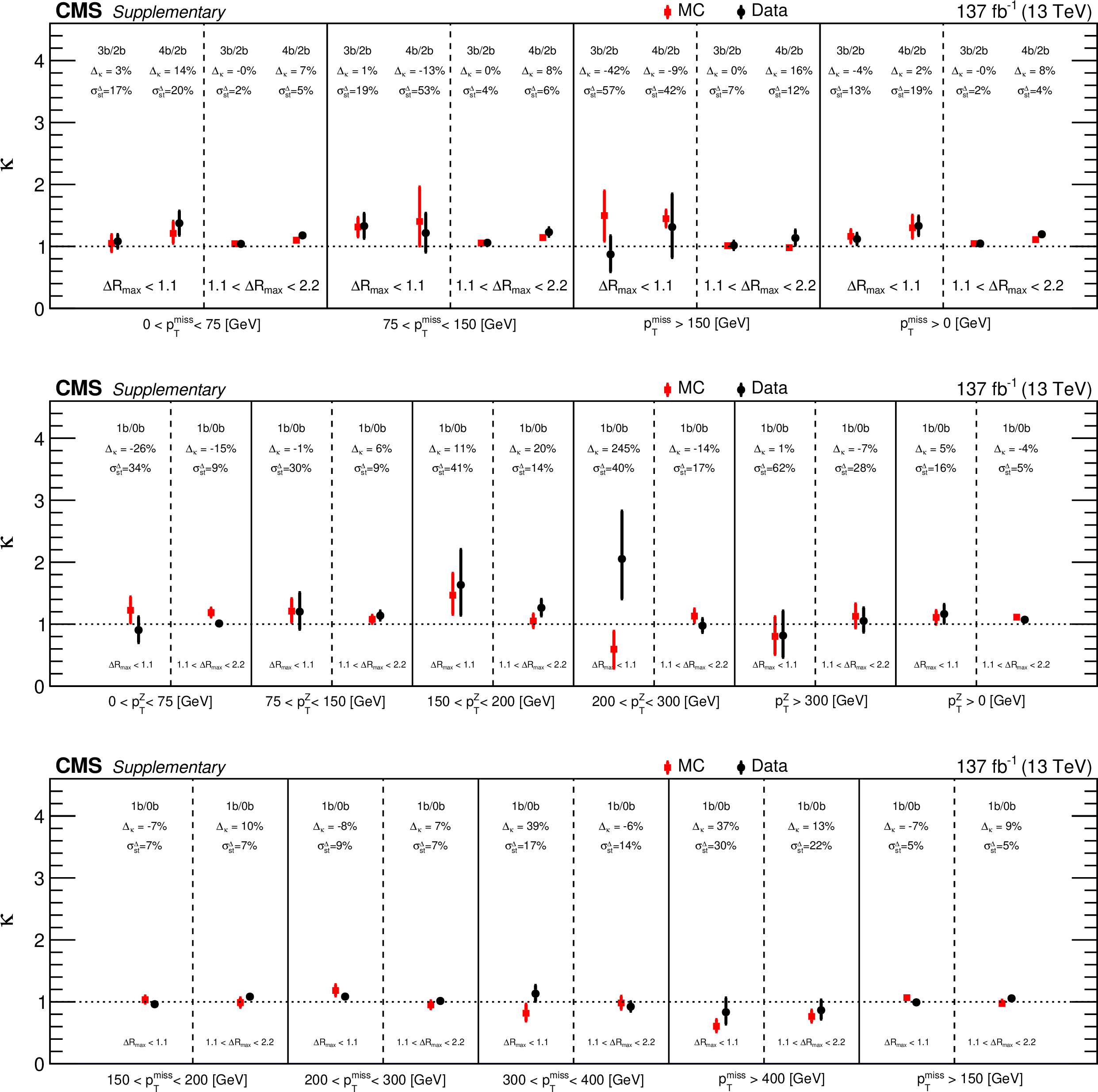
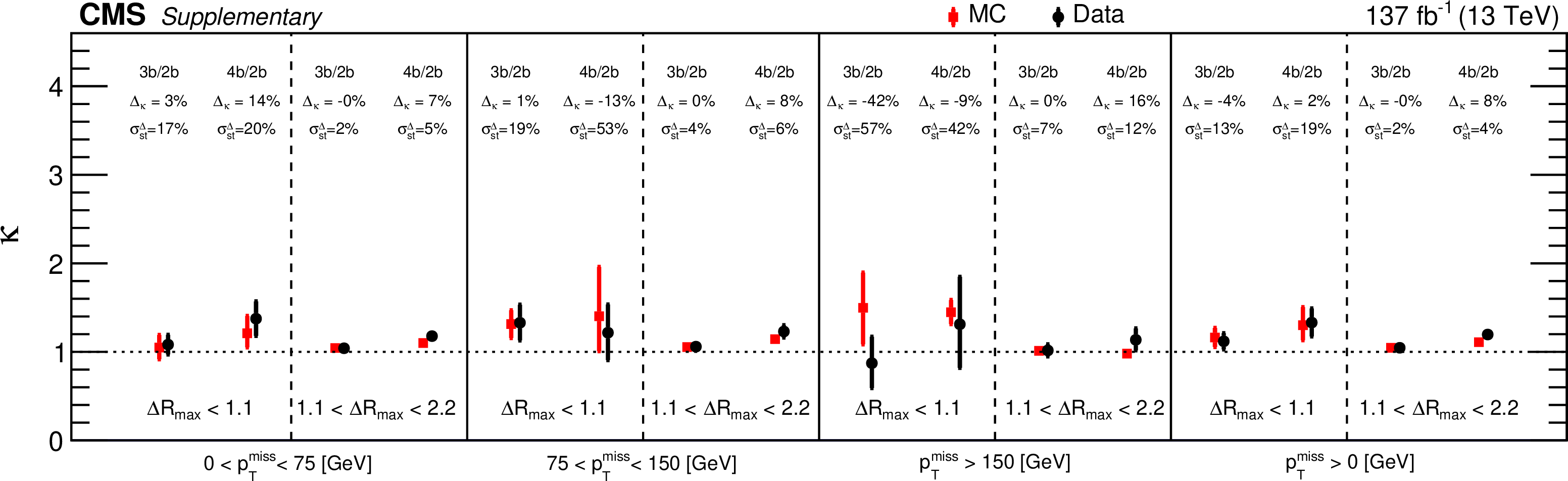
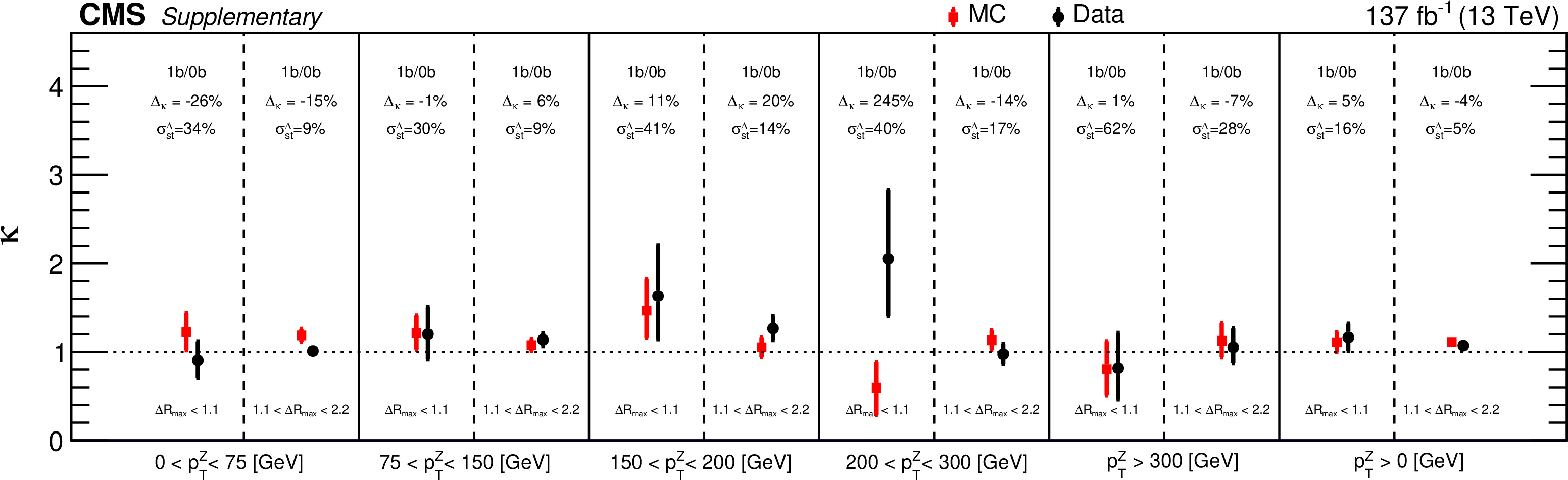
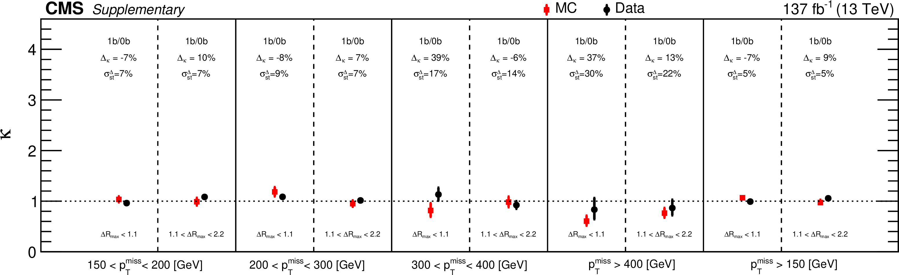
png pdf	Additional Figure 12: Comparison of the value of $\kappa = (N_\text {SR}/N_\text {SB})/(N_\text {CSR}/N_\text {CSB})$, for the resolved signature, between SM simulation and data for the 1-lepton control sample (a), the 2-lepton control sample (b), and the low-$\Delta \phi $ control sample (c). The values of $\Delta _\kappa $ refer to the difference between the value of $\kappa $ in data and simulation. The symbol $\sigma _\text {stat}$ refers to the statistical uncertainty of the value of $\kappa $ measured in data relative to unity.
png pdf	Additional Figure 12-a: Comparison of the value of $\kappa = (N_\text {SR}/N_\text {SB})/(N_\text {CSR}/N_\text {CSB})$, for the resolved signature, between SM simulation and data for the 1-lepton control sample. The values of $\Delta _\kappa $ refer to the difference between the value of $\kappa $ in data and simulation. The symbol $\sigma _\text {stat}$ refers to the statistical uncertainty of the value of $\kappa $ measured in data relative to unity.
png pdf	Additional Figure 12-b: Comparison of the value of $\kappa = (N_\text {SR}/N_\text {SB})/(N_\text {CSR}/N_\text {CSB})$, for the resolved signature, between SM simulation and data for the 2-lepton control sample. The values of $\Delta _\kappa $ refer to the difference between the value of $\kappa $ in data and simulation. The symbol $\sigma _\text {stat}$ refers to the statistical uncertainty of the value of $\kappa $ measured in data relative to unity.
png pdf	Additional Figure 12-c: Comparison of the value of $\kappa = (N_\text {SR}/N_\text {SB})/(N_\text {CSR}/N_\text {CSB})$, for the resolved signature, between SM simulation and data for the low-$\Delta \phi $ control sample. The values of $\Delta _\kappa $ refer to the difference between the value of $\kappa $ in data and simulation. The symbol $\sigma _\text {stat}$ refers to the statistical uncertainty of the value of $\kappa $ measured in data relative to unity.
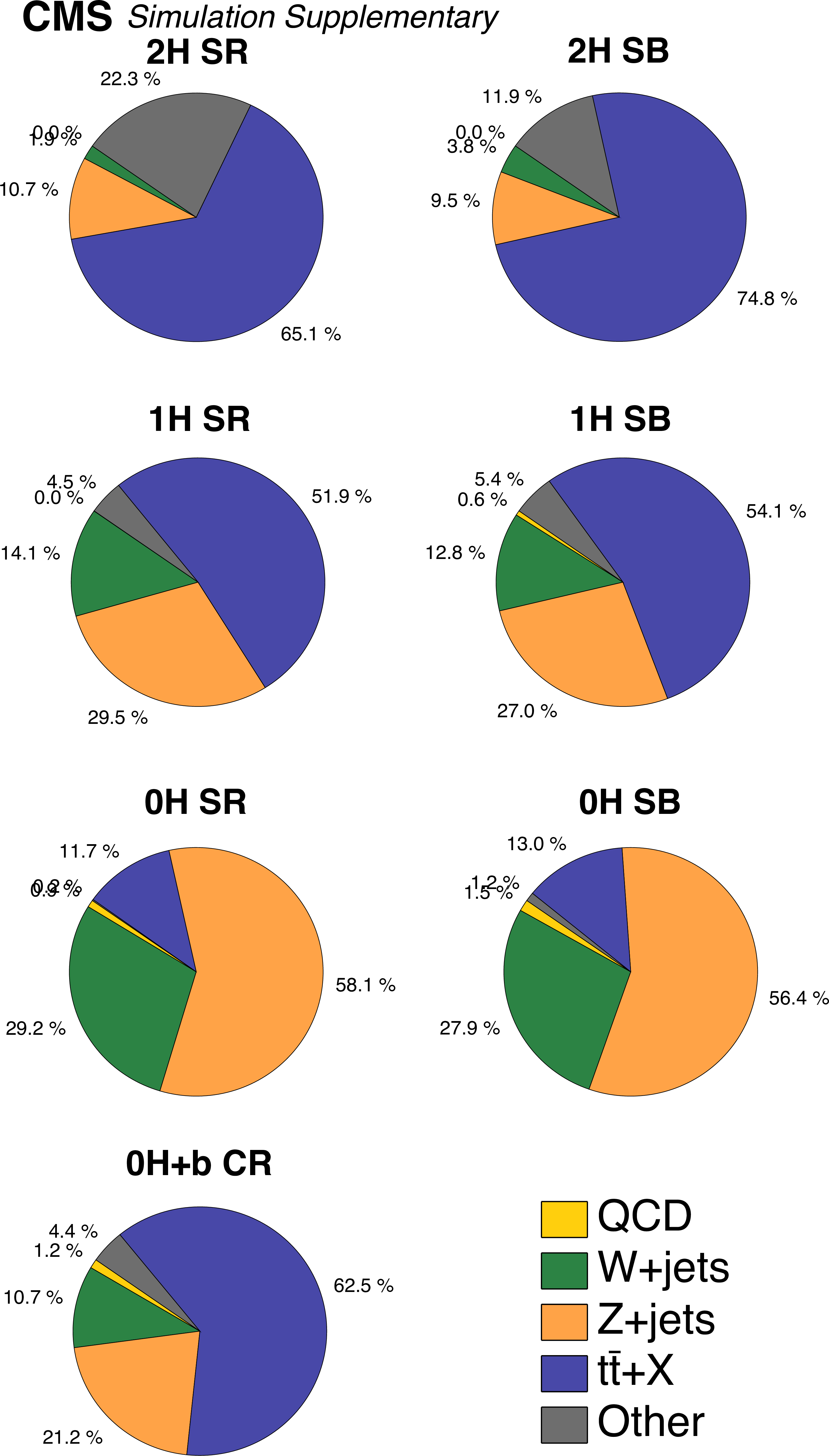
png pdf	Additional Figure 13: The background composition in each of the six analysis regions for the boosted topology, integrated over ${{p_{\mathrm {T}}} ^\text {miss}}$, for $N_{\mathrm {H}}= $ 2 (top), $N_{\mathrm {H}} = $ 1 (second row), and $N_{\mathrm {H}}= $ 0 (third row). The left column shows the three regions with jets in the mass window (95-145 GeV), (C)SR, while the right column shows the three regions in the mass sideband (60-95 GeV) and (145-260 GeV), (C)SB. The bottom left is for the "0H+b" region.
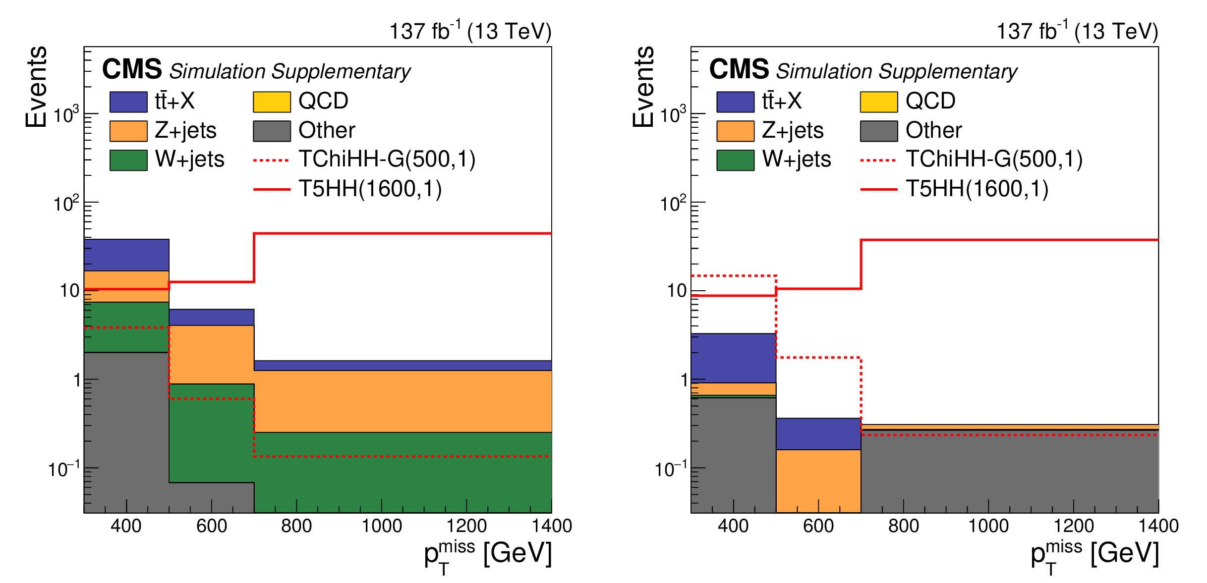
png pdf	Additional Figure 14: Distributions in ${{p_{\mathrm {T}}} ^\text {miss}}$ for the (a) $N_{\mathrm {H}} = $ 1 and (b) $N_{\mathrm {H}}= $ 2 signal regions of the boosted phase space, from the simulation (filled histograms). Two signal points, one each for the TChiHH-G and T5HH signal samples, are shown by the red dotted and solid lines.
png pdf	Additional Figure 14-a: Distributions in ${{p_{\mathrm {T}}} ^\text {miss}}$ for the $N_{\mathrm {H}} = $ 1 signal region of the boosted phase space, from the simulation (filled histograms). Two signal points, one each for the TChiHH-G and T5HH signal samples, are shown by the red dotted and solid lines.
png pdf	Additional Figure 14-b: Distributions in ${{p_{\mathrm {T}}} ^\text {miss}}$ for the $N_{\mathrm {H}}= $ 2 signal region of the boosted phase space, from the simulation (filled histograms). Two signal points, one each for the TChiHH-G and T5HH signal samples, are shown by the red dotted and solid lines.
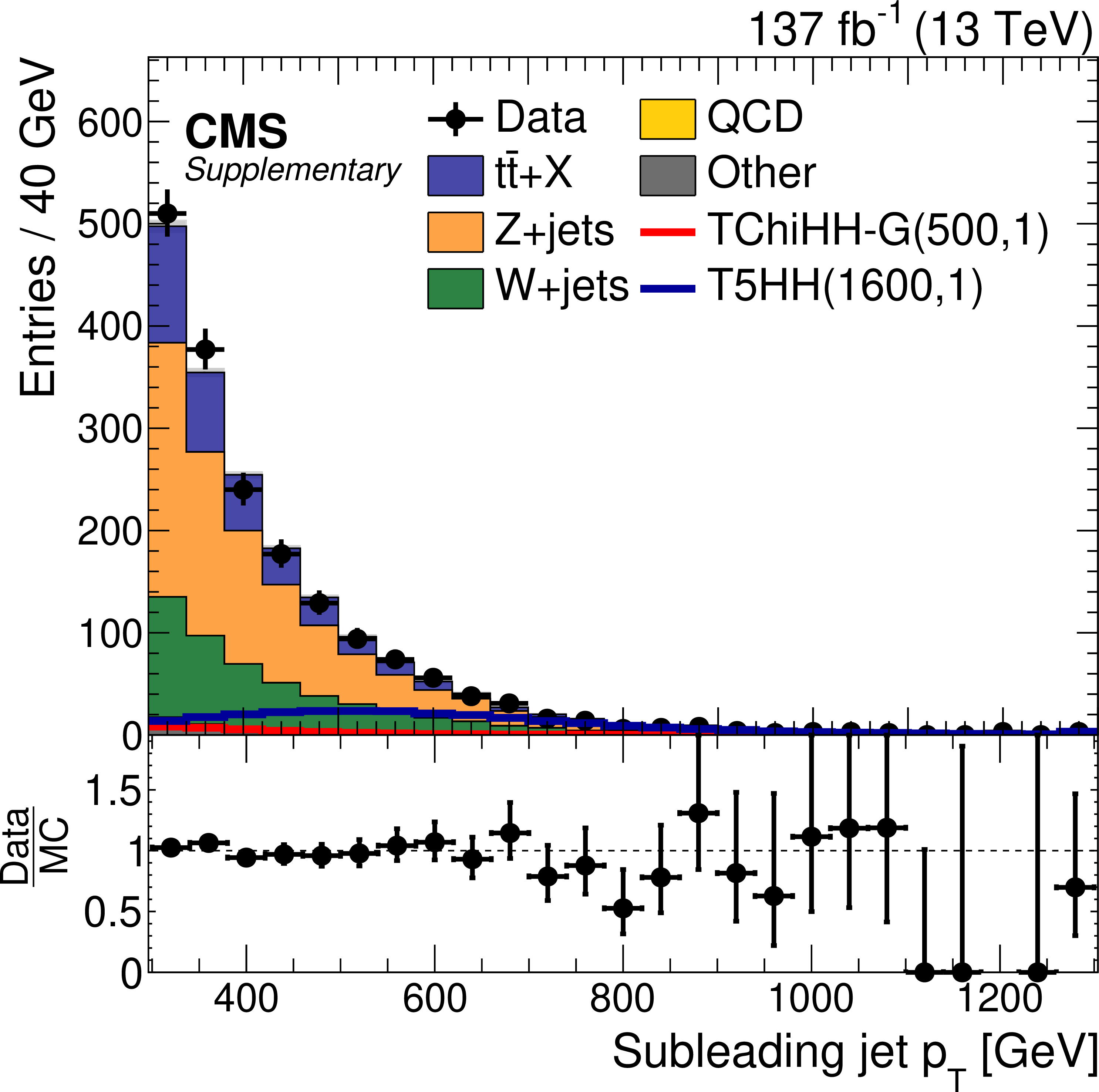
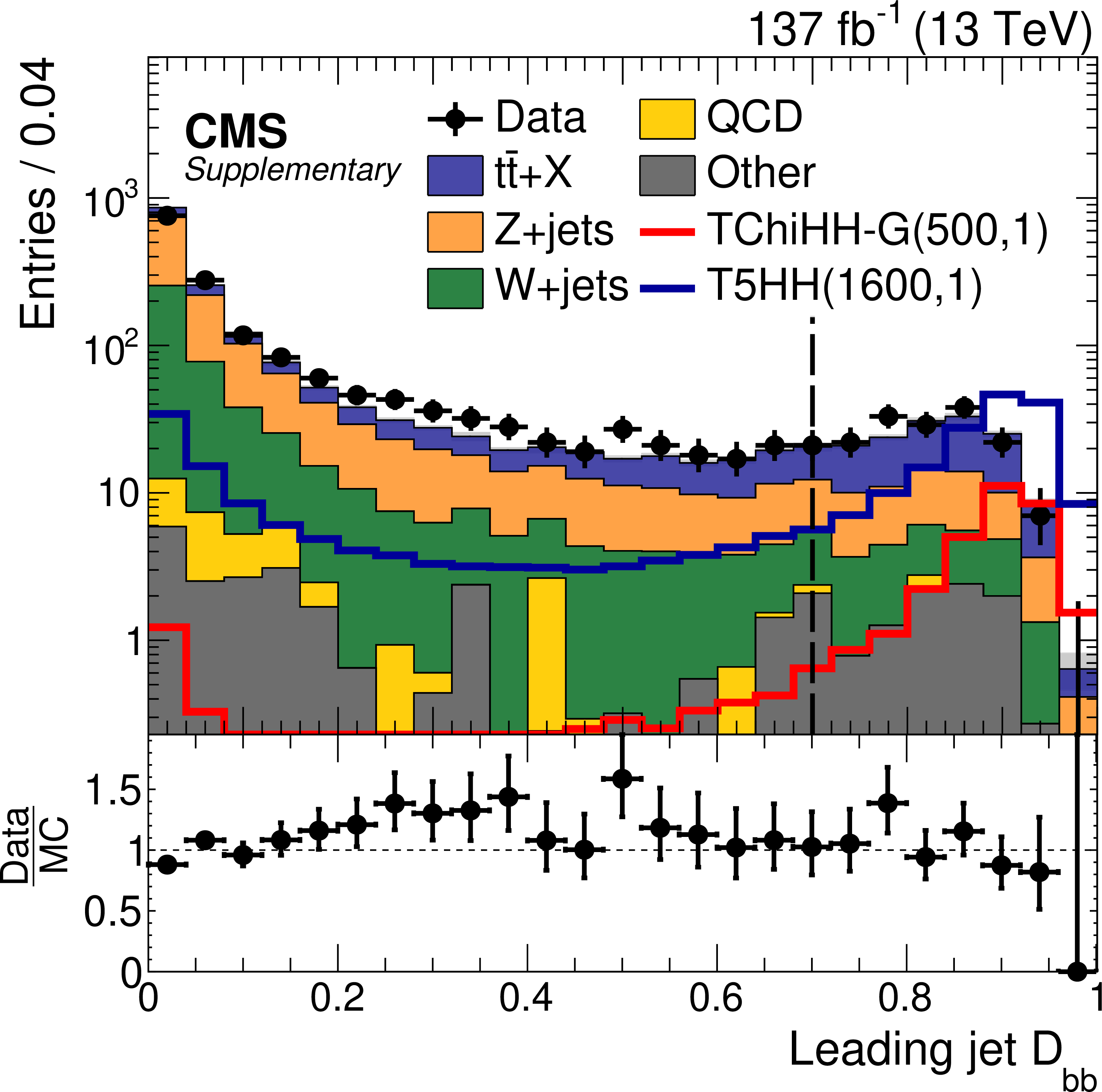
png pdf	Additional Figure 15: Distributions for the (a, c, and e) leading- and (b, d, and f) subleading-$ {p_{\mathrm {T}}}$ jet, in the most pertinent variables for the boosted signature. The baseline requirements are applied, except for those on the variable shown. The variables are (a, b) $ {p_{\mathrm {T}}}$, (c, d) $D_{{\mathrm{b} \mathrm{b}}}$, and (e, f) $m_{J}$. The SM backgrounds from simulation are scaled by 86% to match the data integral. Two signal points, a mass point for the TChiHH-G and one for the T5HH signal samples, are shown. The lower panel in each plot shows the ratio of observed to (scaled) simulated yields.
png pdf	Additional Figure 15-a: Distribution of $ {p_{\mathrm {T}}}$ for the leading-$ {p_{\mathrm {T}}}$ jet. The baseline requirements are applied, except for those on the variable shown. The SM backgrounds from simulation are scaled by 86% to match the data integral. Two signal points, a mass point for the TChiHH-G and one for the T5HH signal samples, are shown. The lower panel shows the ratio of observed to (scaled) simulated yields.
png pdf	Additional Figure 15-b: Distribution of $ {p_{\mathrm {T}}}$ for the subleading-$ {p_{\mathrm {T}}}$ jet. The baseline requirements are applied, except for those on the variable shown. The SM backgrounds from simulation are scaled by 86% to match the data integral. Two signal points, a mass point for the TChiHH-G and one for the T5HH signal samples, are shown. The lower panel shows the ratio of observed to (scaled) simulated yields.
png pdf	Additional Figure 15-c: Distribution of $D_{{\mathrm{b} \mathrm{b}}}$ for the leading-$ {p_{\mathrm {T}}}$ jet. The baseline requirements are applied, except for those on the variable shown. The SM backgrounds from simulation are scaled by 86% to match the data integral. Two signal points, a mass point for the TChiHH-G and one for the T5HH signal samples, are shown. The lower panel shows the ratio of observed to (scaled) simulated yields.
png pdf	Additional Figure 15-d: Distribution of $D_{{\mathrm{b} \mathrm{b}}}$ for the subleading-$ {p_{\mathrm {T}}}$ jet. The baseline requirements are applied, except for those on the variable shown. The SM backgrounds from simulation are scaled by 86% to match the data integral. Two signal points, a mass point for the TChiHH-G and one for the T5HH signal samples, are shown. The lower panel shows the ratio of observed to (scaled) simulated yields.
png pdf	Additional Figure 15-e: Distribution of $m_{J}$ for the leading-$ {p_{\mathrm {T}}}$ jet. The baseline requirements are applied, except for those on the variable shown. The SM backgrounds from simulation are scaled by 86% to match the data integral. Two signal points, a mass point for the TChiHH-G and one for the T5HH signal samples, are shown. The lower panel shows the ratio of observed to (scaled) simulated yields.
png pdf	Additional Figure 15-f: Distribution of $m_{J}$ for the subleading-$ {p_{\mathrm {T}}}$ jet. The baseline requirements are applied, except for those on the variable shown. The SM backgrounds from simulation are scaled by 86% to match the data integral. Two signal points, a mass point for the TChiHH-G and one for the T5HH signal samples, are shown. The lower panel shows the ratio of observed to (scaled) simulated yields.
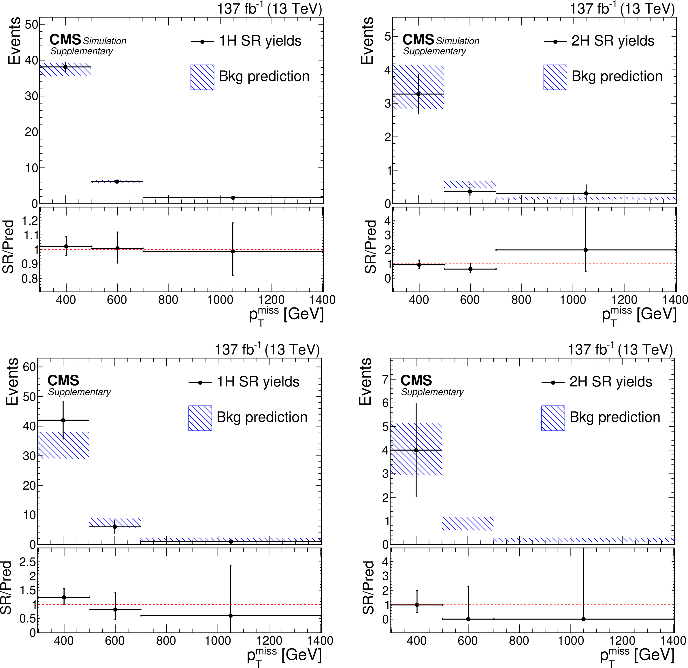
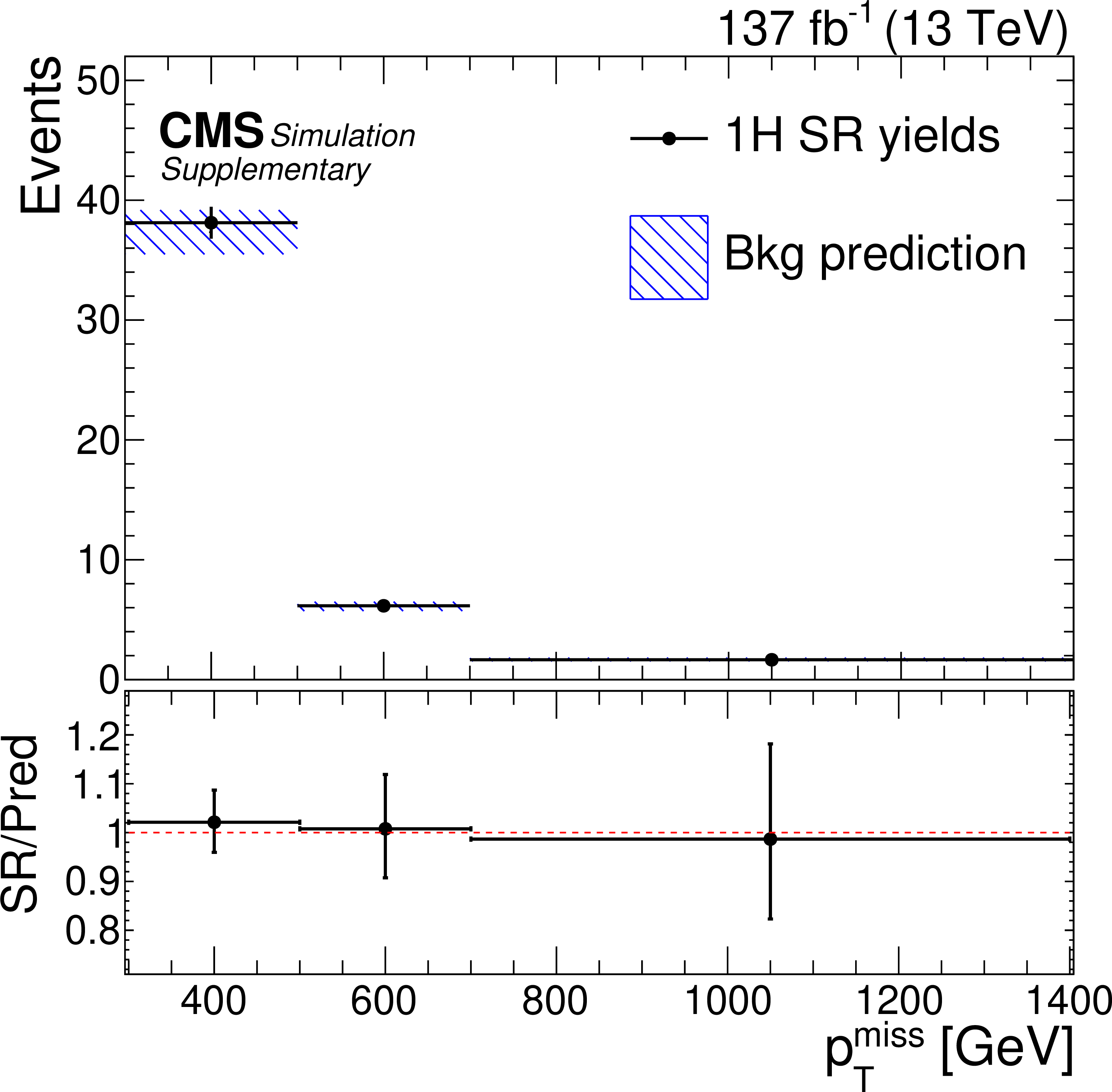
png pdf	Additional Figure 16: The full background estimation method closure for the boosted topology for (a, c) $N_{\mathrm {H}} = $ 1 and (b, d) $N_{\mathrm {H}}= $ 2 signal regions, in both MC (a, b) and data (c, d). The error bars on the background prediction are statistical only.
png pdf	Additional Figure 16-a: The full background estimation method closure for the boosted topology for $N_{\mathrm {H}} = $ 1 signal region, in MC. The error bars on the background prediction are statistical only.
png pdf	Additional Figure 16-b: The full background estimation method closure for the boosted topology for $N_{\mathrm {H}} = $ 2 signal region, in MC. The error bars on the background prediction are statistical only.
png pdf	Additional Figure 16-c: The full background estimation method closure for the boosted topology for $N_{\mathrm {H}} = $ 1 signal region, in data. The error bars on the background prediction are statistical only.
png pdf	Additional Figure 16-d: The full background estimation method closure for the boosted topology for $N_{\mathrm {H}} = $ 2 signal region, in data. The error bars on the background prediction are statistical only.
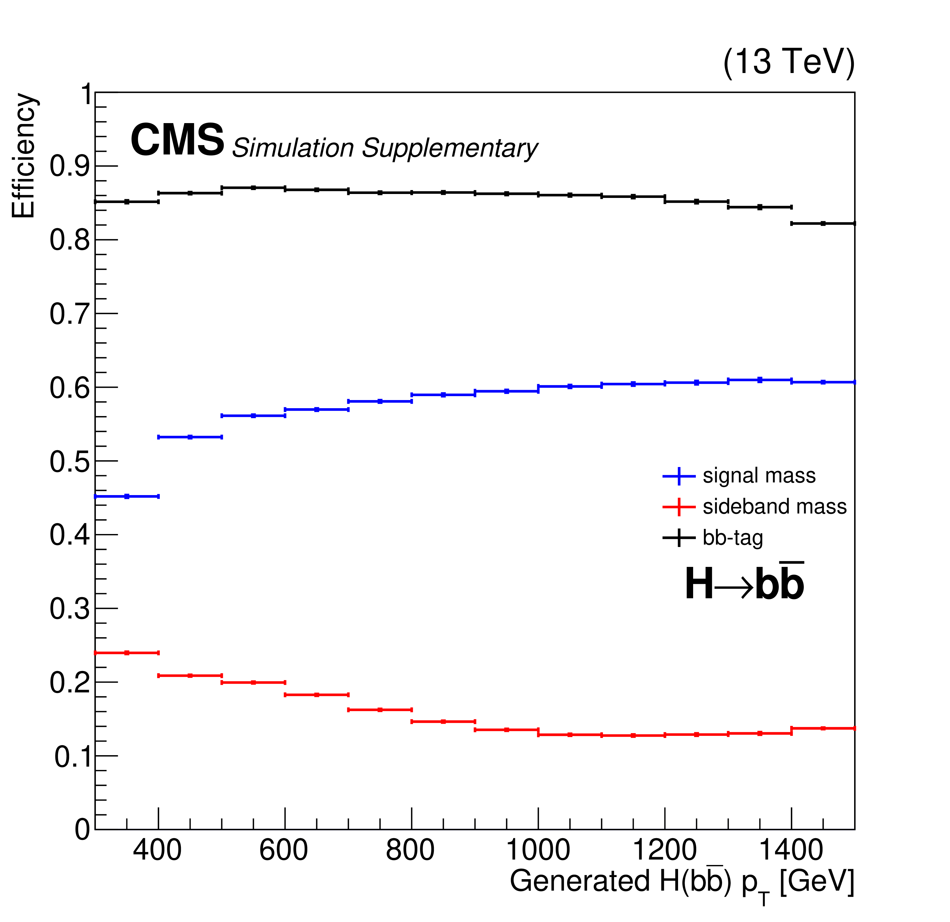
png pdf	Additional Figure 17: Efficiencies for Higgs-matched AK8 jets for $D_{ {\mathrm{b} \mathrm{b}}}$ (black) and the soft-drop mass algorithm (blue and red) for the boosted topology. The mass efficiency of the signal window (95-145 GeV) (blue) and the sideband (60-95 and 145-260 GeV) (red) are relative to the boosted baseline selection, except for the $m_{\mathrm {J}}$ requirement. The $D_{ {\mathrm{b} \mathrm{b}}}$ efficiency is for jets within the signal mass window. The sample considered for this efficiency is a combination of signal mass points in the simplified T5HH model.
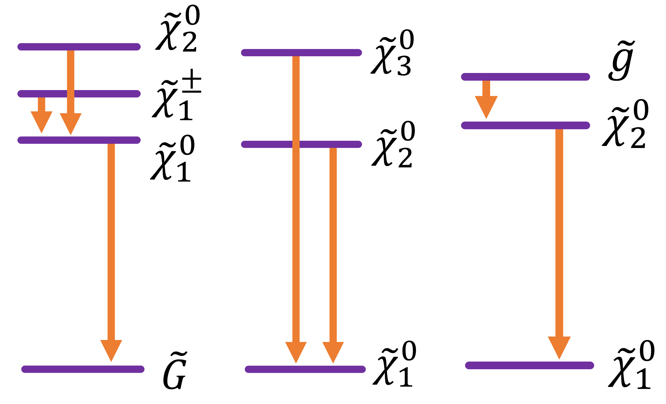
png pdf	Additional Figure 18: Mass hierarchy of the SUSY particles in the simplified SUSY models; (a) TChiHH-G, (b) TChiHH, (c) T5HH.
png pdf	Additional Figure 18-a: Mass hierarchy of the SUSY particles in the simplified SUSY TChiHH-G model.
png pdf	Additional Figure 18-b: Mass hierarchy of the SUSY particles in the simplified SUSY TChiHH model.
png pdf	Additional Figure 18-c: Mass hierarchy of the SUSY particles in the simplified SUSY T5HH model.
png pdf	Additional Figure 19: Signal event topology in an electroweak production scenario.
png pdf	Additional Figure 20: Reconstruction of a Higgs boson as (a) two AK4 jets, and (b) one AK8 jet.
png pdf	Additional Figure 20-a: Reconstruction of a Higgs boson as two AK4 jets.
png pdf	Additional Figure 20-b: Reconstruction of a Higgs boson as one AK4 jet.
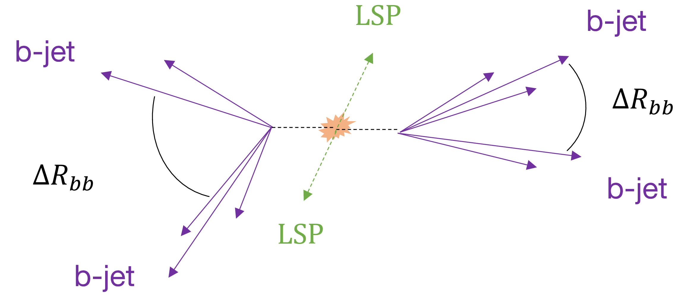
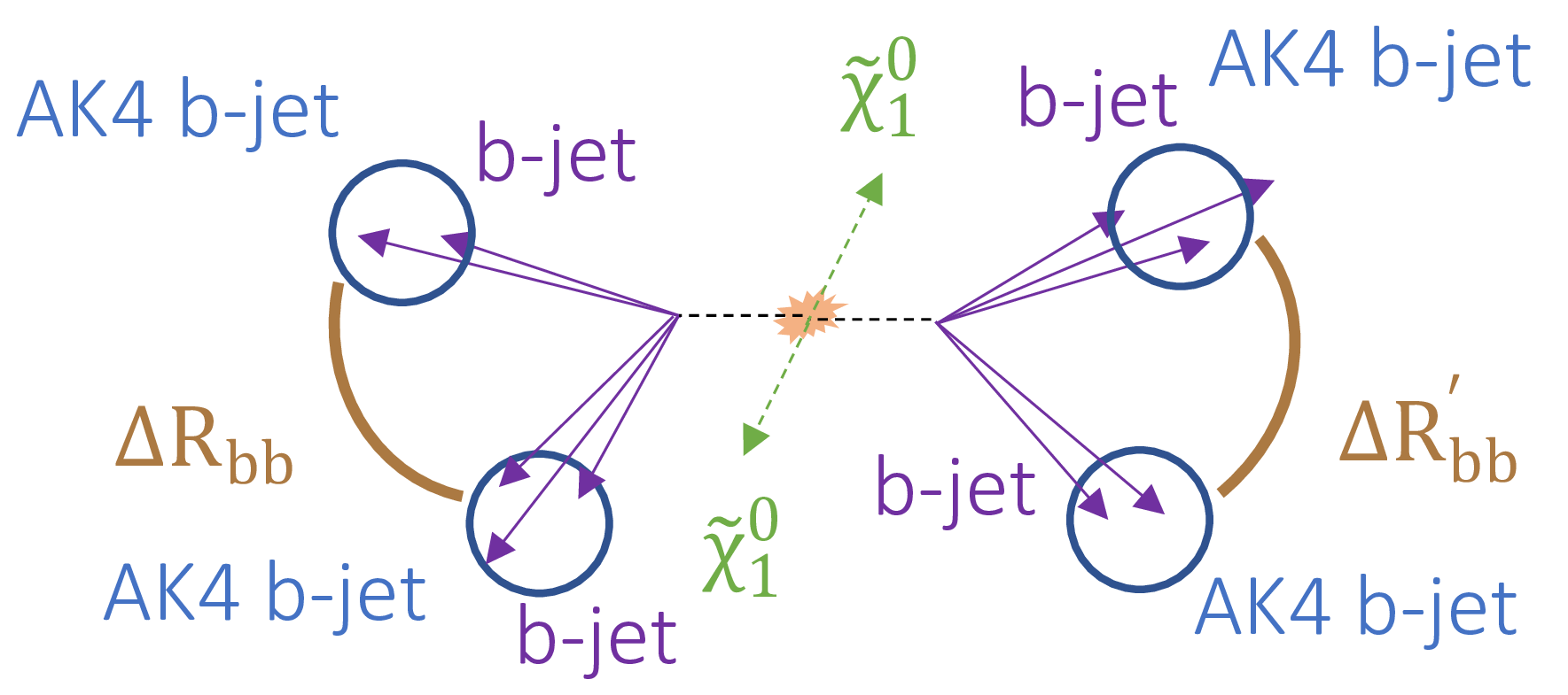
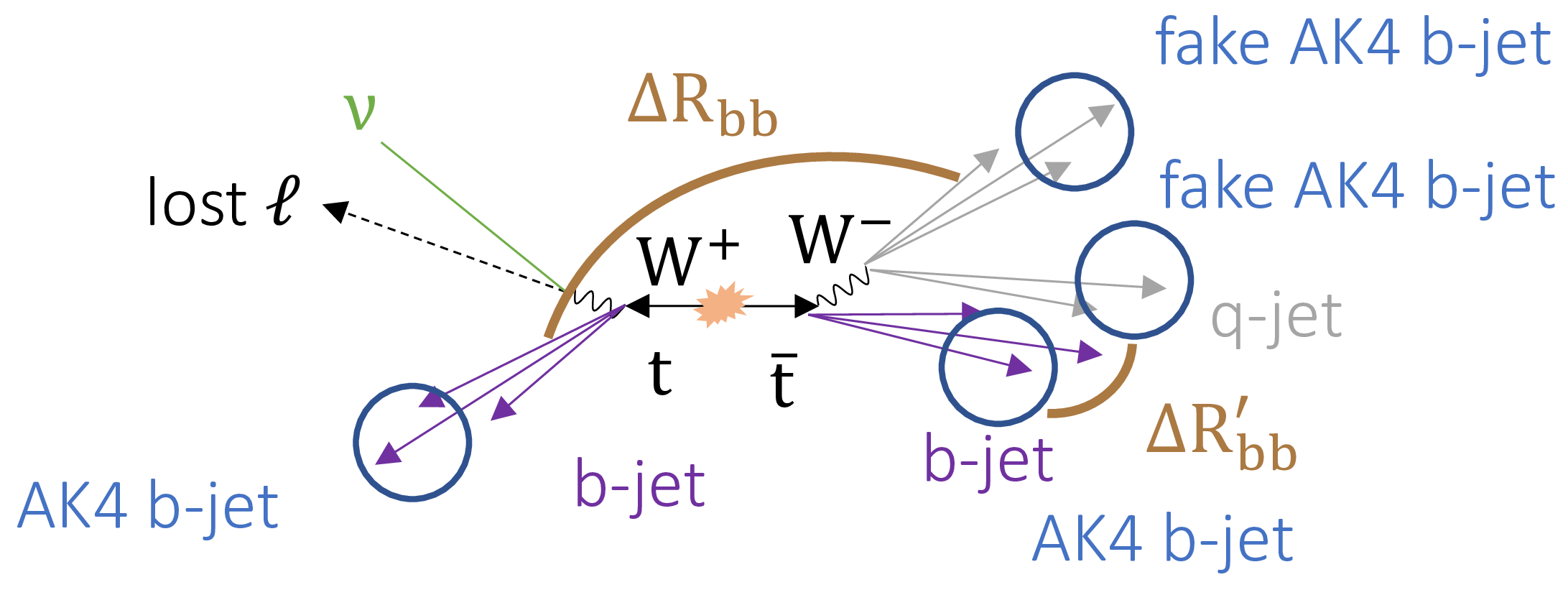
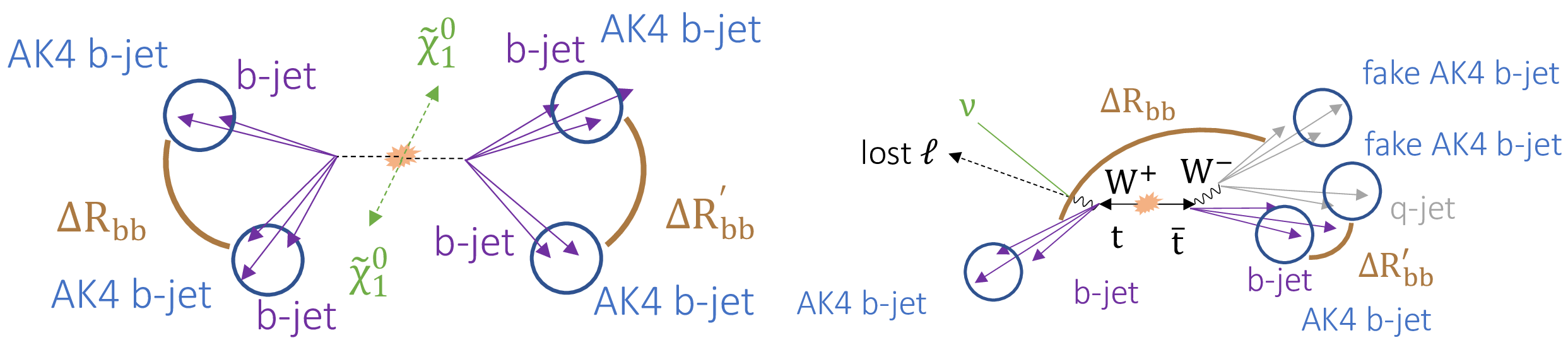
png pdf	Additional Figure 21: Typical configuration of (a) signal and (b) ${\mathrm{t} \mathrm{\bar{t}}}$ events with the resolved signature. In ${\mathrm{t} \mathrm{\bar{t}}}$ events, the presence of a misidentified b jet often results in a large value of $\Delta R_{bb}$ for one of the Higgs boson candidates.
png pdf	Additional Figure 21-a: Typical configuration of signal events with the resolved signature.
png pdf	Additional Figure 21-b: Typical configuration of signal ${\mathrm{t} \mathrm{\bar{t}}}$ events with the resolved signature. The presence of a misidentified b jet often results in a large value of $\Delta R_{bb}$ for one of the Higgs boson candidates.
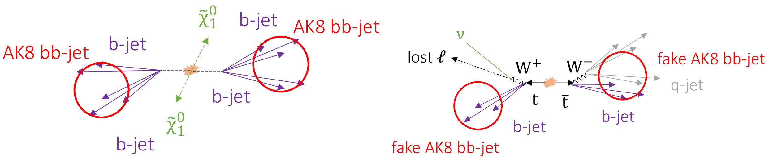
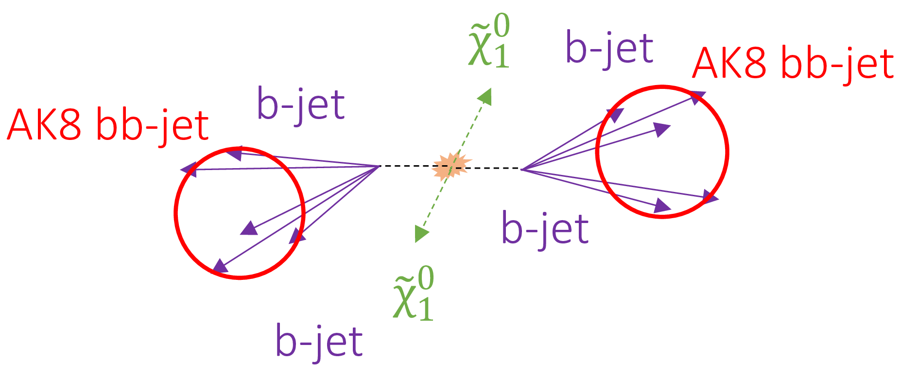
png pdf	Additional Figure 22: Typical configuration of (a) signal and (b) background events with the boosted signature.
png pdf	Additional Figure 22-a: Typical configuration of signal events with the boosted signature.
png pdf	Additional Figure 22-b: Typical configuration of background events with the boosted signature.
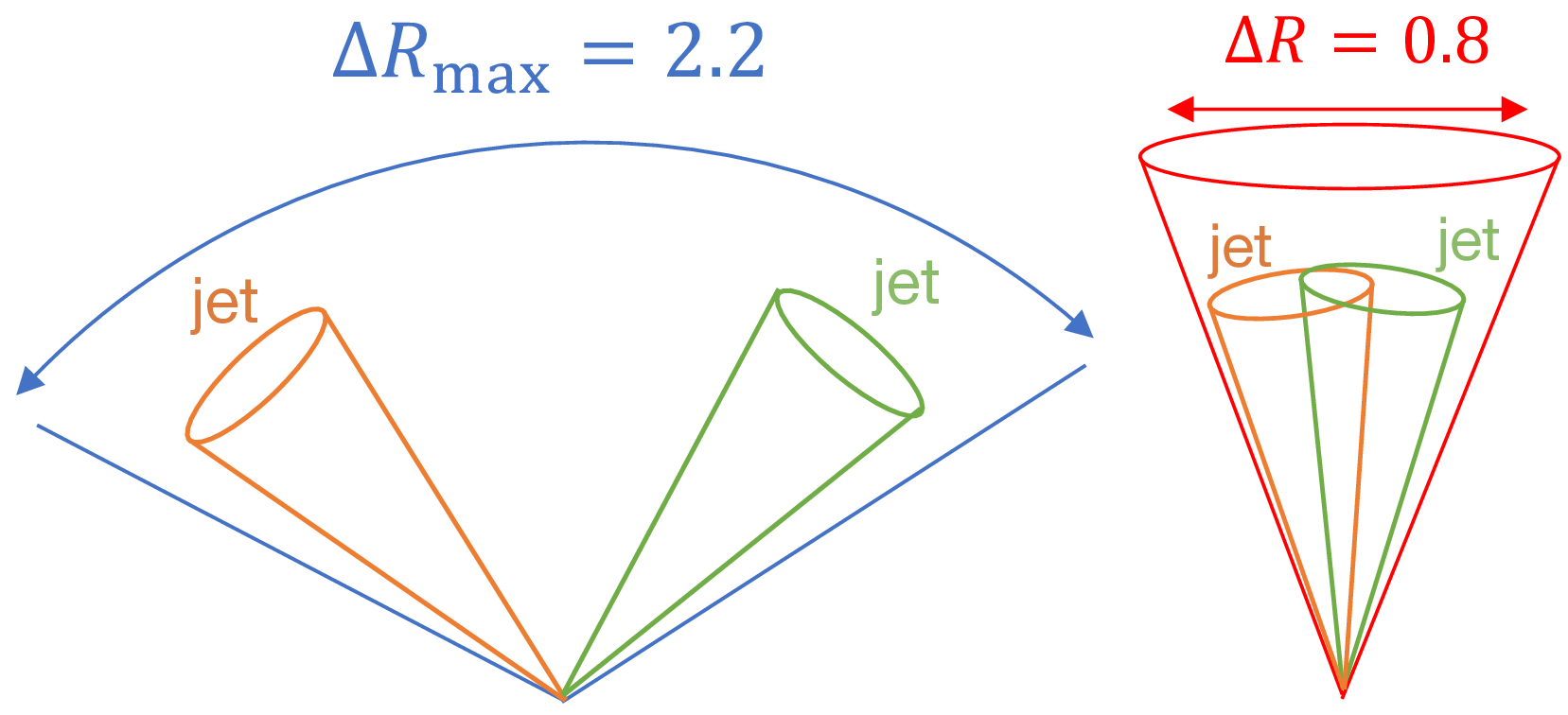
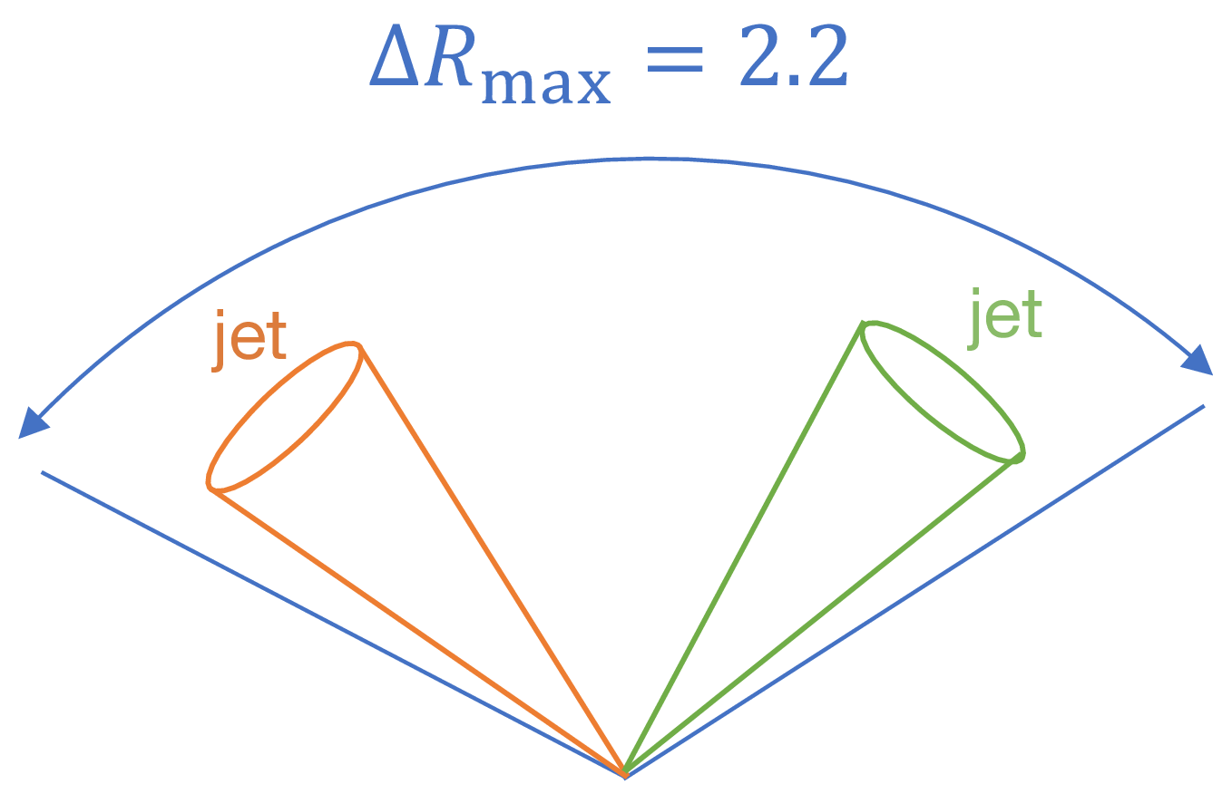
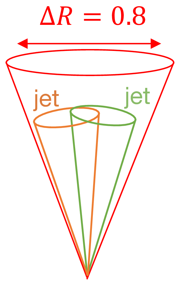
png pdf	Additional Figure 23: Two dimensional distribution in simulated signal events (950 GeV higgsinos) of $\Delta R_{\mathrm{b} \mathrm{\bar{b}}}$ for the leading and subleading Higgs boson candidates, showing the approximate phase-space coverage of the resolved and boosted searches. The resolved phase space region extends from $\Delta R_{\mathrm{b} \mathrm{\bar{b}}} = $ 0.4 to 2.2, corresponding to the middle of the histogram, while the lower left part of the plot corresponds to the boosted phase space region.
png pdf	Additional Figure 24: Analysis regions used for the (left) resolved and (right) boosted signatures, after the baseline selection requirements are applied. The signal and sideband regions used for the background estimation are indicated. Further binning in other kinematic variables is applied.
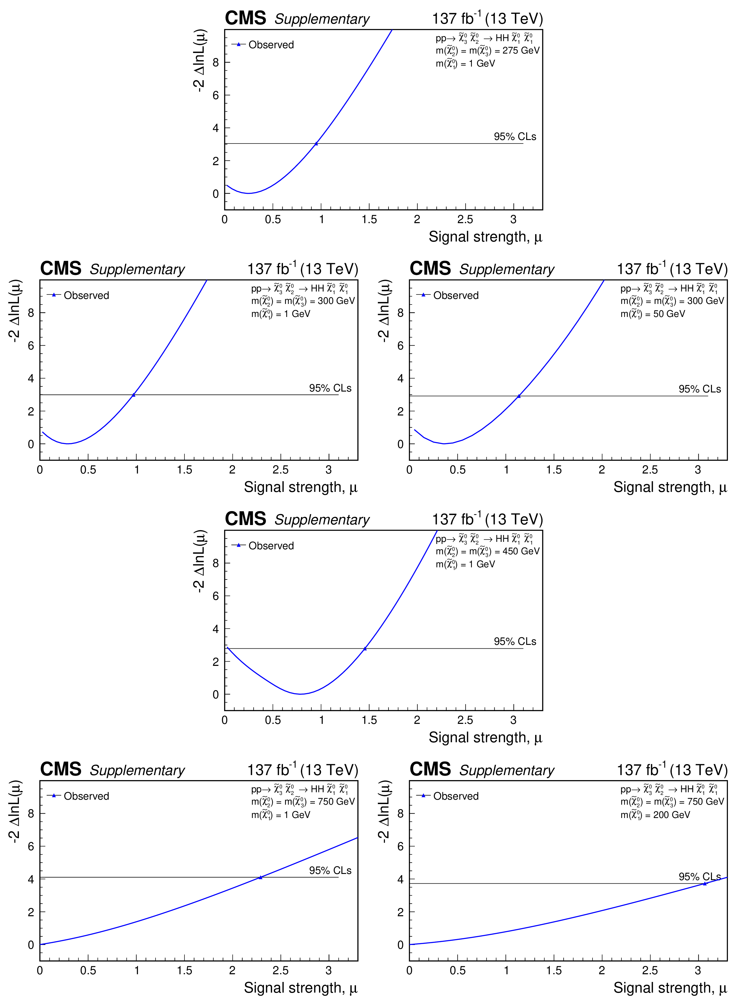
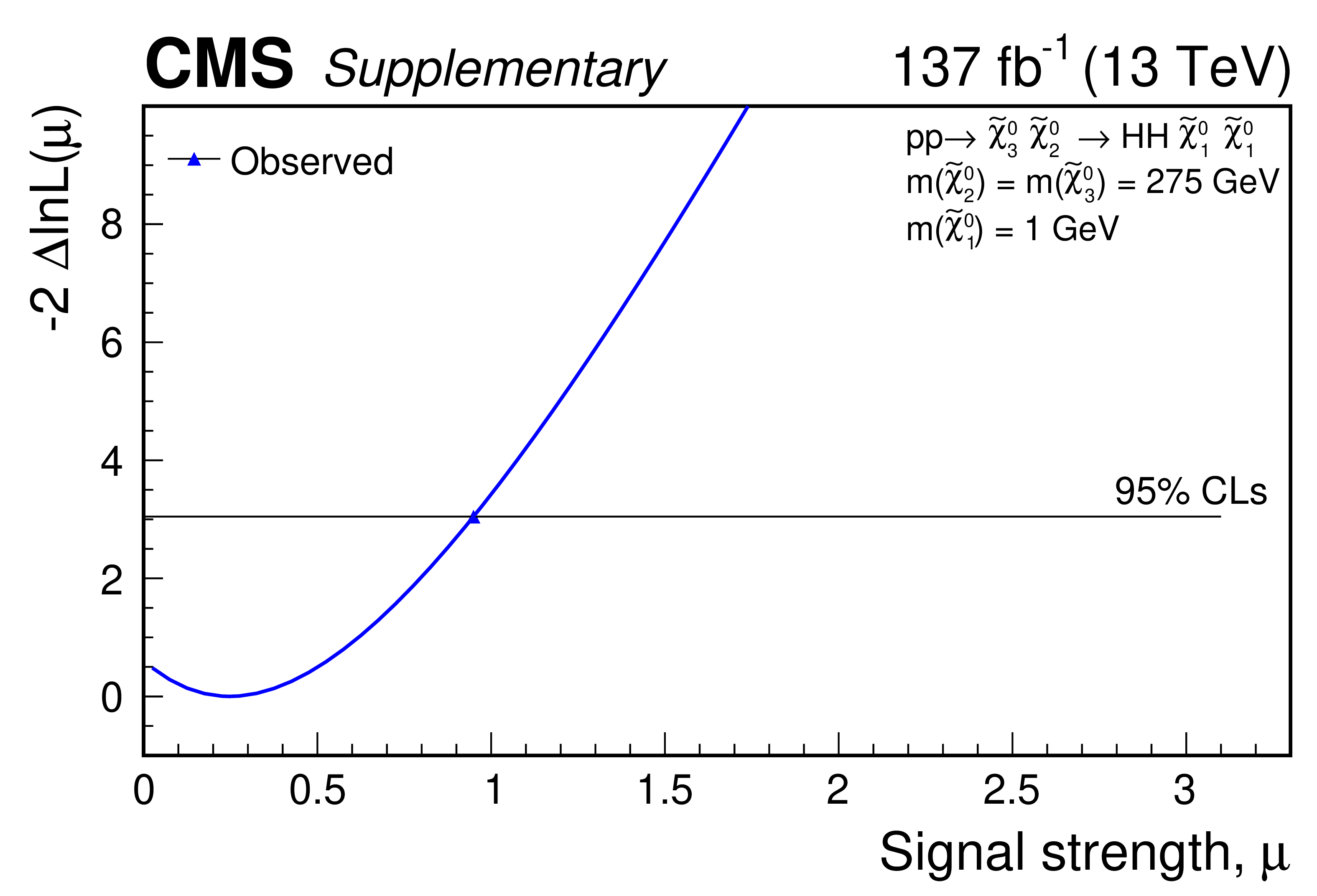
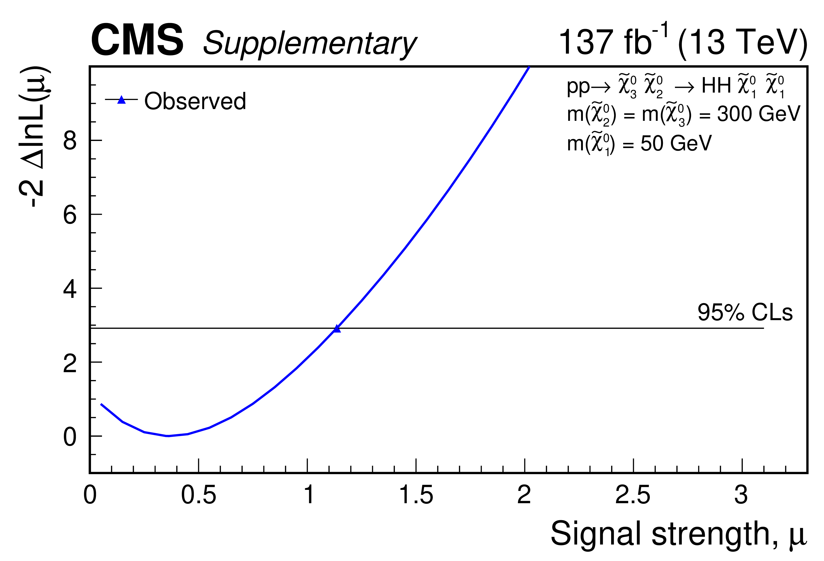
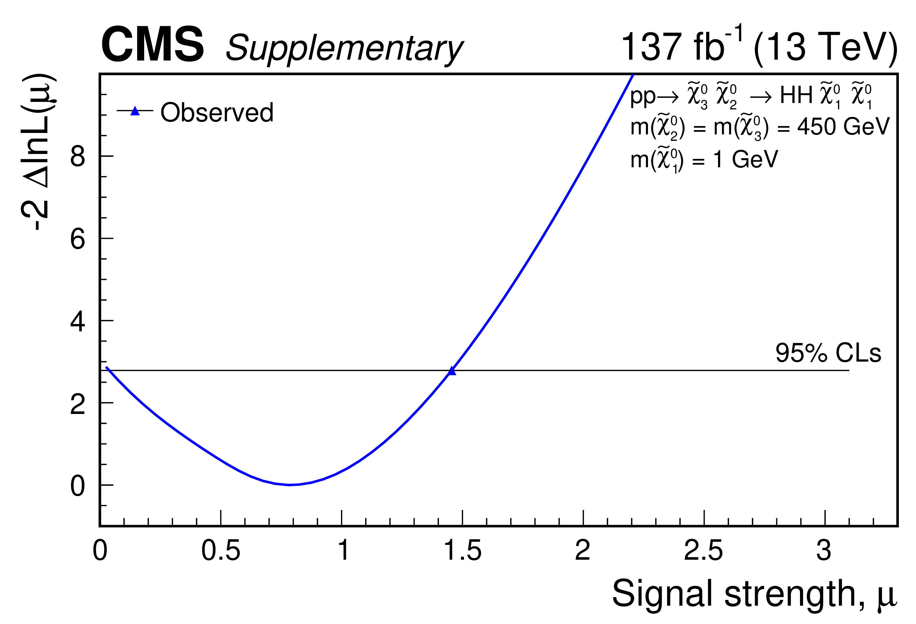
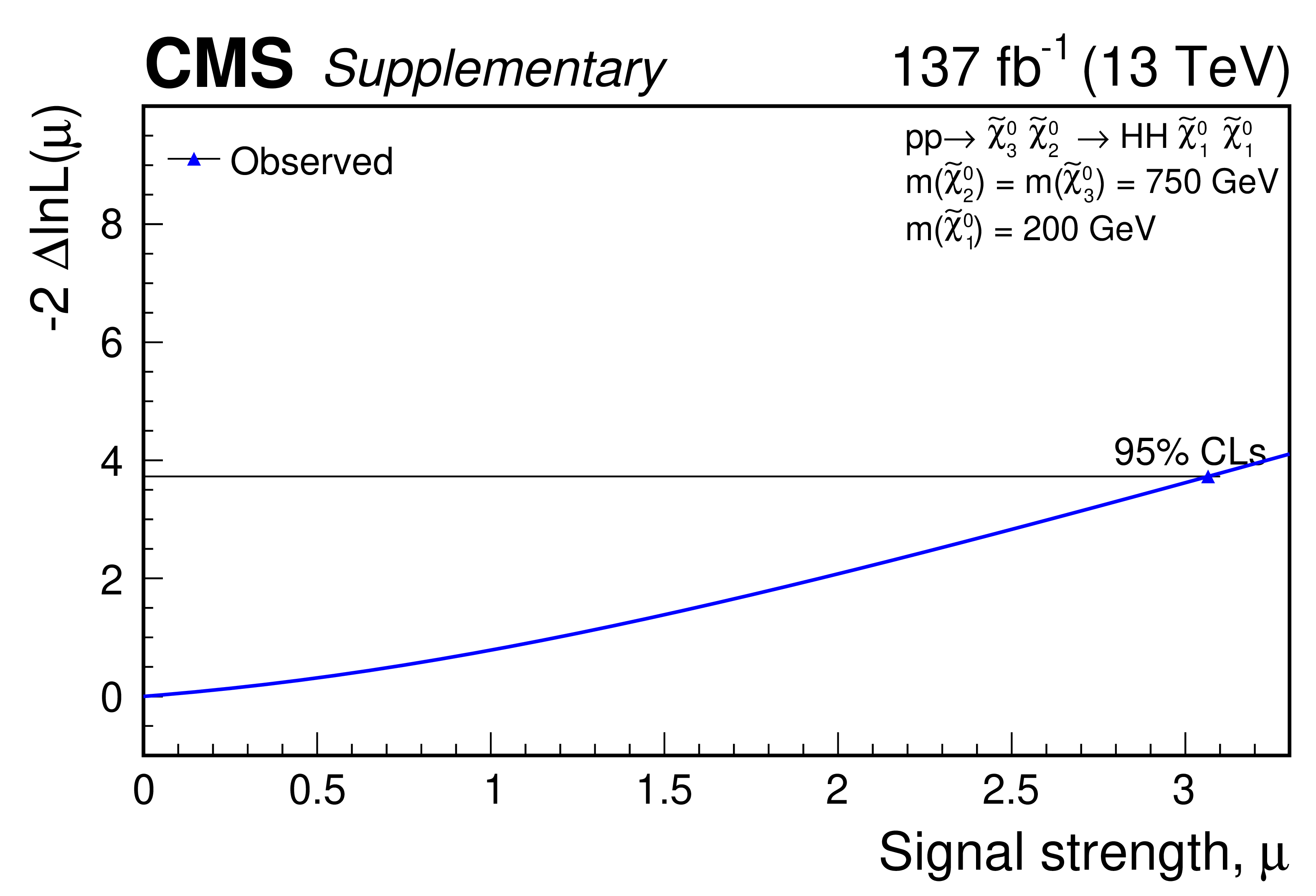
png pdf	Additional Figure 25: Profile likelihood functions for representative scan points for the TChiHH model.
png pdf	Additional Figure 25-a: Profile likelihood function for a representative scan point for the TChiHH model.
png pdf	Additional Figure 25-b: Profile likelihood function for a representative scan point for the TChiHH model.
png pdf	Additional Figure 25-c: Profile likelihood function for a representative scan point for the TChiHH model.
png pdf	Additional Figure 25-d: Profile likelihood function for a representative scan point for the TChiHH model.
png pdf	Additional Figure 25-e: Profile likelihood function for a representative scan point for the TChiHH model.
png pdf	Additional Figure 25-f: Profile likelihood function for a representative scan point for the TChiHH model.

Additional Tables
png pdf	Additional Table 1: Signal event efficiencies of the resolved topology for the TChiHH model with a 450 GeV higgsino mass and 1 GeV LSP mass. The denominator for the efficiency calculation includes only $\mathrm{H} \to \mathrm{b} \mathrm{\bar{b}} $ decays.
png pdf	Additional Table 2: Signal event efficiencies of the boosted topology for the T5HH model with a 2200 GeV gluino mass.
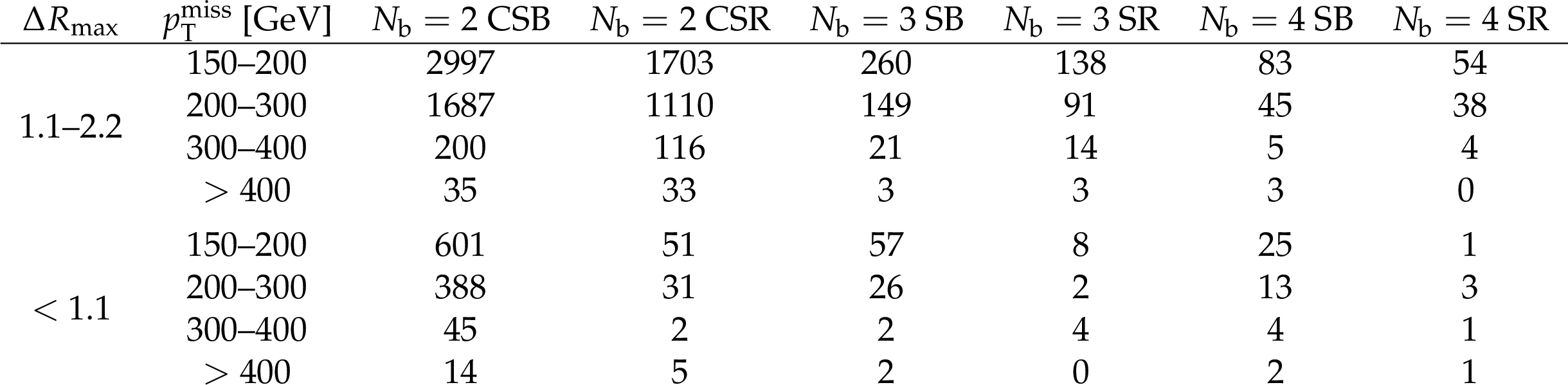
png pdf	Additional Table 3: Resolved results table, including the data yields in the 6 ABCD regions in each ${{p_{\mathrm {T}}} ^\text {miss}}$ -$\Delta R_{\text {max}}$ plane.
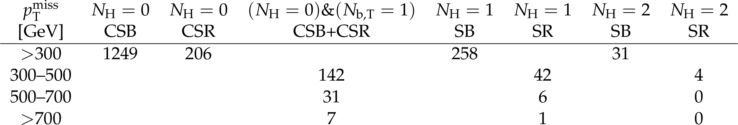
png pdf	Additional Table 4: Boosted results table, including the data yields in the 6 analysis ABCD regions in each ${{p_{\mathrm {T}}} ^\text {miss}}$ bin. The data yields for the 0H+b control region, used to determine the ${{p_{\mathrm {T}}} ^\text {miss}}$ shape, are also included.
png pdf	Additional Table 5: Cut flow table for the resolved topology showing expected event yields at 137 fb$^{-1}$ for selected signal models as successive selections are applied. The selections above the horizontal line correspond to the resolved topology baseline selection.
png pdf	Additional Table 6: Cut flow table for the boosted topology showing expected event yields at 137 fb$^{-1}$ for selected signal models as successive selections are applied. Here the hadronic baseline is defined by $N_{\mathrm {jet}}\geq $2, ${{p_{\mathrm {T}}} ^\text {miss}}$ $ > $300 GeV, $\Delta \phi $ cuts, and the isolated lepton and track vetoes.

References
1	ATLAS Collaboration	Observation of a new particle in the search for the standard model Higgs boson with the ATLAS detector at the LHC	PLB 716 (2012) 1	1207.7214
2	CMS Collaboration	Observation of a new boson at a mass of 125 GeV with the CMS experiment at the LHC	PLB 716 (2012) 30	CMS-HIG-12-028 1207.7235
3	CMS Collaboration	Observation of a new boson with mass near 125 GeV in pp collisions at $ \sqrt{s} = $ 7 and 8 TeV	JHEP 06 (2013) 081	CMS-HIG-12-036 1303.4571
4	ATLAS and CMS Collaborations	Combined measurement of the Higgs boson mass in pp collisions at $ \sqrt{s}= $ 7 and 8 TeV with the ATLAS and CMS experiments	PRL 114 (2015) 191803	1503.07589
5	P. Ramond	Dual theory for free fermions	PRD 3 (1971) 2415
6	Y. A. Golfand and E. P. Likhtman	Extension of the algebra of Poincaré group generators and violation of P invariance	JEPTL 13 (1971)323
7	A. Neveu and J. H. Schwarz	Factorizable dual model of pions	NPB 31 (1971) 86
8	D. V. Volkov and V. P. Akulov	Possible universal neutrino interaction	JEPTL 16 (1972)438
9	J. Wess and B. Zumino	A Lagrangian model invariant under supergauge transformations	PLB 49 (1974) 52
10	J. Wess and B. Zumino	Supergauge transformations in four dimensions	NPB 70 (1974) 39
11	P. Fayet	Supergauge invariant extension of the Higgs mechanism and a model for the electron and its neutrino	NPB 90 (1975) 104
12	P. Fayet and S. Ferrara	Supersymmetry	PR 32 (1977) 249
13	H. P. Nilles	Supersymmetry, supergravity and particle physics	Phys. Rep. 110 (1984) 1
14	S. P. Martin	A supersymmetry primer	Adv. Ser. Direct. High Energy Phys. 21 (2010) 1	hep-ph/9709356
15	S. Dimopoulos and G. F. Giudice	Naturalness constraints in supersymmetric theories with nonuniversal soft terms	PLB 357 (1995) 573	hep-ph/9507282
16	R. Barbieri and D. Pappadopulo	S-particles at their naturalness limits	JHEP 10 (2009) 061	0906.4546
17	M. Papucci, J. T. Ruderman, and A. Weiler	Natural SUSY endures	JHEP 09 (2012) 035	1110.6926
18	LHC Higgs Cross Section Working Group	Handbook of LHC Higgs cross sections: 4. deciphering the nature of the Higgs sector	CERN (2016)	1610.07922
19	ATLAS Collaboration	Search for supersymmetry in events with photons, bottom quarks, and missing transverse momentum in proton-proton collisions at a centre-of-mass energy of 7 TeV with the ATLAS detector	PLB 719 (2013) 261	1211.1167
20	ATLAS Collaboration	Search for direct pair production of a chargino and a neutralino decaying to the 125 GeV Higgs boson in $ \sqrt{s} = $ 8 TeV pp collisions with the ATLAS detector	EPJC 75 (2015) 208	1501.07110
21	ATLAS Collaboration	Search for supersymmetry in final states with two same-sign or three leptons and jets using 36 fb$ ^{-1} $ of $ \sqrt{s}= $ 13 TeV pp collision data with the ATLAS detector	JHEP 09 (2017) 084	1706.03731
22	ATLAS Collaboration	Search for new phenomena with large jet multiplicities and missing transverse momentum using large-radius jets and flavour-tagging at ATLAS in 13 TeV pp collisions	JHEP 12 (2017) 034	1708.02794
23	ATLAS Collaboration	Search for squarks and gluinos in events with an isolated lepton, jets, and missing transverse momentum at $ \sqrt{s}= $ 13 TeV with the ATLAS detector	PRD 96 (2017) 112010	1708.08232
24	ATLAS Collaboration	Search for squarks and gluinos in final states with jets and missing transverse momentum using 36 fb$ ^{-1} $ of $ \sqrt{s}= $ 13 TeV pp collision data with the ATLAS detector	PRD 97 (2018) 112001	1712.02332
25	ATLAS Collaboration	Search for electroweak production of supersymmetric states in scenarios with compressed mass spectra at $ \sqrt{s}= $ 13 TeV with the ATLAS detector	PRD 97 (2018) 052010	1712.08119
26	ATLAS Collaboration	Search for photonic signatures of gauge-mediated supersymmetry in 13 TeV pp collisions with the ATLAS detector	PRD 97 (2018) 092006	1802.03158
27	ATLAS Collaboration	Search for electroweak production of supersymmetric particles in final states with two or three leptons at $ \sqrt{s}= $ 13 TeV with the ATLAS detector	EPJC 78 (2018) 995	1803.02762
28	ATLAS Collaboration	Search for chargino-neutralino production using recursive jigsaw reconstruction in final states with two or three charged leptons in proton-proton collisions at $ \sqrt{s}= $ 13 TeV with the ATLAS detector	PRD 98 (2018) 092012	1806.02293
29	ATLAS Collaboration	Search for pair production of higgsinos in final states with at least three $ b $-tagged jets in $ \sqrt{s} = $ 13 TeV pp collisions using the ATLAS detector	PRD 98 (2018) 092002	1806.04030
30	ATLAS Collaboration	Search for chargino and neutralino production in final states with a Higgs boson and missing transverse momentum at $ \sqrt{s} = $ 13 TeV with the ATLAS detector	PRD 100 (2019) 012006	1812.09432
31	ATLAS Collaboration	Search for electroweak production of charginos and sleptons decaying into final states with two leptons and missing transverse momentum in $ \sqrt{s}= $ 13 TeV pp collisions using the ATLAS detector	EPJC 80 (2020) 123	1908.08215
32	ATLAS Collaboration	Search for direct production of electroweakinos in final states with one lepton, missing transverse momentum and a Higgs boson decaying into two $ b $-jets in pp collisions at $ \sqrt{s}= $ 13 TeV with the ATLAS detector	EPJC 80 (2020) 691	1909.09226
33	ATLAS Collaboration	Searches for electroweak production of supersymmetric particles with compressed mass spectra in $ \sqrt{s}= $ 13 TeV pp collisions with the ATLAS detector	PRD 101 (2020) 052005	1911.12606
34	ATLAS Collaboration	Search for chargino-neutralino production with mass splittings near the electroweak scale in three-lepton final states in $ \sqrt {s} = $ 13 TeV pp collisions with the ATLAS detector	PRD 101 (2020) 072001	1912.08479
35	ATLAS Collaboration	Search for direct production of electroweakinos in final states with missing transverse momentum and a Higgs boson decaying into photons in pp collisions at $ \sqrt{s} = $ 13 TeV with the ATLAS detector	JHEP 10 (2020) 005	2004.10894
36	ATLAS Collaboration	Search for supersymmetry in events with four or more charged leptons in 139 fb$^{-1}$ of $ \sqrt{s}= $ 13 TeV pp collisions with the ATLAS detector	JHEP 07 (2021) 167	2103.11684
37	ATLAS Collaboration	Search for charginos and neutralinos in final states with two boosted hadronically decaying bosons and missing transverse momentum in pp collisions at $ \sqrt{s}= $ 13 TeV with the ATLAS detector	PRD 104 (2021), no. 11, 112010	2108.07586
38	CMS Collaboration	Searches for electroweak production of charginos, neutralinos, and sleptons decaying to leptons and W, Z, and Higgs bosons in pp collisions at 8 TeV	EPJC 74 (2014) 3036	CMS-SUS-13-006 1405.7570
39	CMS Collaboration	Search for top squark and higgsino production using diphoton Higgs boson decays	PRL 112 (2014) 161802	CMS-SUS-13-014 1312.3310
40	CMS Collaboration	Searches for electroweak neutralino and chargino production in channels with Higgs, Z, and W bosons in pp collisions at 8 TeV	PRD 90 (2014) 092007	CMS-SUS-14-002 1409.3168
41	CMS Collaboration	Search for physics beyond the standard model in events with two leptons of same sign, missing transverse momentum, and jets in proton-proton collisions at $ \sqrt{s} = $ 13 TeV	EPJC 77 (2017) 578	CMS-SUS-16-035 1704.07323
42	CMS Collaboration	Search for electroweak production of charginos and neutralinos in WH events in proton-proton collisions at $ \sqrt{s}= $ 13 TeV	JHEP 11 (2017) 029	CMS-SUS-16-043 1706.09933
43	CMS Collaboration	Search for supersymmetry in events with at least one photon, missing transverse momentum, and large transverse event activity in proton-proton collisions at $ \sqrt{s}= $ 13 TeV	JHEP 12 (2017) 142	CMS-SUS-16-047 1707.06193
44	CMS Collaboration	Search for supersymmetry with Higgs boson to diphoton decays using the razor variables at $ \sqrt{s} = $ 13 TeV	PLB 779 (2018) 166	CMS-SUS-16-045 1709.00384
45	CMS Collaboration	Search for higgsino pair production in pp collisions at $ \sqrt{s} = $ 13 TeV in final states with large missing transverse momentum and two Higgs bosons decaying via $\mathrm{ H \to b \bar b }$	PRD 97 (2018) 032007	CMS-SUS-16-044 1709.04896
46	CMS Collaboration	Combined search for electroweak production of charginos and neutralinos in proton-proton collisions at $ \sqrt{s} = $ 13 TeV	JHEP 03 (2018) 160	CMS-SUS-17-004 1801.03957
47	CMS Collaboration	Search for new phenomena in final states with two opposite-charge, same-flavor leptons, jets, and missing transverse momentum in pp collisions at $ \sqrt{s}= $ 13 TeV	JHEP 03 (2018) 076	CMS-SUS-16-034 1709.08908
48	CMS Collaboration	Search for supersymmetry in events with one lepton and multiple jets exploiting the angular correlation between the lepton and the missing transverse momentum in proton-proton collisions at $ \sqrt{s} = $ 13 TeV	PLB 780 (2018) 384	CMS-SUS-16-042 1709.09814
49	CMS Collaboration	Search for supersymmetry in events with at least three electrons or muons, jets, and missing transverse momentum in proton-proton collisions at $ \sqrt{s}= $ 13 TeV	JHEP 02 (2018) 067	CMS-SUS-16-041 1710.09154
50	CMS Collaboration	Search for gauge-mediated supersymmetry in events with at least one photon and missing transverse momentum in pp collisions at $ \sqrt{s} = $ 13 TeV	PLB 780 (2018) 118	CMS-SUS-16-046 1711.08008
51	CMS Collaboration	Search for physics beyond the standard model in events with high-momentum Higgs bosons and missing transverse momentum in proton-proton collisions at 13 TeV	PRL 120 (2018) 241801	CMS-SUS-17-006 1712.08501
52	CMS Collaboration	Search for new physics in events with two soft oppositely charged leptons and missing transverse momentum in proton-proton collisions at $ \sqrt{s}= $ 13 TeV	PLB 782 (2018) 440	CMS-SUS-16-048 1801.01846
53	CMS Collaboration	Searches for pair production of charginos and top squarks in final states with two oppositely charged leptons in proton-proton collisions at $ \sqrt{s}= $ 13 TeV	JHEP 11 (2018) 079	CMS-SUS-17-010 1807.07799
54	CMS Collaboration	Search for supersymmetry in events with a photon, a lepton, and missing transverse momentum in proton-proton collisions at $ \sqrt{s} = $ 13 TeV	JHEP 01 (2019) 154	CMS-SUS-17-012 1812.04066
55	CMS Collaboration	Search for supersymmetry in events with a photon, jets, b-jets, and missing transverse momentum in proton-proton collisions at 13 TeV	EPJC 79 (2019) 444	CMS-SUS-18-002 1901.06726
56	CMS Collaboration	Search for supersymmetry in final states with photons and missing transverse momentum in proton-proton collisions at 13 TeV	JHEP 06 (2019) 143	CMS-SUS-17-011 1903.07070
57	CMS Collaboration	Combined search for supersymmetry with photons in proton-proton collisions at $ \sqrt{s}= $ 13 TeV	PLB 801 (2020) 135183	CMS-SUS-18-005 1907.00857
58	CMS Collaboration	Search for supersymmetry using Higgs boson to diphoton decays at $ \sqrt{s} = $ 13 TeV	JHEP 11 (2019) 109	CMS-SUS-18-007 1908.08500
59	CMS Collaboration	Searches for physics beyond the standard model with the $ M_\mathrm{T2} $ variable in hadronic final states with and without disappearing tracks in proton-proton collisions at $ \sqrt{s}= $ 13 TeV	EPJC 80 (2020) 3	CMS-SUS-19-005 1909.03460
60	CMS Collaboration	Search for physics beyond the standard model in events with jets and two same-sign or at least three charged leptons in proton-proton collisions at $ \sqrt{s}= $ 13 TeV	EPJC 80 (2020) 752	CMS-SUS-19-008 2001.10086
61	CMS Collaboration	Search for supersymmetry in proton-proton collisions at $ \sqrt{s} = $ 13 TeV in events with high-momentum Z bosons and missing transverse momentum	JHEP 09 (2020) 149	CMS-SUS-19-013 2008.04422
62	CMS Collaboration	Search for supersymmetry in final states with two oppositely charged same-flavor leptons and missing transverse momentum in proton-proton collisions at $ \sqrt{s} = $ 13 TeV	JHEP 04 (2021) 123	CMS-SUS-20-001 2012.08600
63	CMS Collaboration	Search for electroweak production of charginos and neutralinos in proton-proton collisions at $ \sqrt{s} = $ 13 TeV	JHEP 04 (2022) 147	CMS-SUS-19-012 2106.14246
64	CMS Collaboration	Search for chargino-neutralino production in events with Higgs and W bosons using 137 fb$ ^{-1} $ of proton-proton collisions at $ \sqrt{s} = $ 13 TeV	JHEP 10 (2021) 045	CMS-SUS-20-003 2107.12553
65	CMS Collaboration	HEPData record for this analysis	link
66	Particle Data Group, P. A. Zyla et al.	Review of particle physics	Prog. Theor. Exp. Phys. 2020 (2020) 083C01
67	G. R. Farrar and P. Fayet	Phenomenology of the production, decay, and detection of new hadronic states associated with supersymmetry	PLB 76 (1978) 575
68	N. Arkani-Hamed et al.	MARMOSET: The path from LHC data to the new standard model via on-shell effective theories		hep-ph/0703088
69	J. Alwall, P. Schuster, and N. Toro	Simplified models for a first characterization of new physics at the LHC	PRD 79 (2009) 075020	0810.3921
70	J. Alwall, M.-P. Le, M. Lisanti, and J. G. Wacker	Model-independent jets plus missing energy searches	PRD 79 (2009) 015005	0809.3264
71	D. Alves et al.	Simplified models for LHC new physics searches	JPG 39 (2012) 105005	1105.2838
72	S. Dimopoulos, M. Dine, S. Raby, and S. D. Thomas	Experimental signatures of low-energy gauge mediated supersymmetry breaking	PRL 76 (1996) 3494	hep-ph/9601367
73	K. T. Matchev and S. D. Thomas	Higgs and Z boson signatures of supersymmetry	PRD 62 (2000) 077702	hep-ph/9908482
74	J. T. Ruderman and D. Shih	General neutralino NLSPs at the early LHC	JHEP 08 (2012) 159	1103.6083
75	B. Fuks, M. Klasen, D. R. Lamprea, and M. Rothering	Gaugino production in proton-proton collisions at a center-of-mass energy of 8 TeV	JHEP 10 (2012) 081	1207.2159
76	B. Fuks, M. Klasen, D. R. Lamprea, and M. Rothering	Precision predictions for electroweak superpartner production at hadron colliders with Resummino	EPJC 73 (2013) 2480	1304.0790
77	H. Baer et al.	Natural SUSY with a bino- or wino-like LSP	PRD 91 (2015) 075005	1501.06357
78	Z. Kang, P. Ko, and J. Li	New physics opportunities in the boosted di-Higgs-boson plus missing transverse energy signature	PRL 116 (2016) 131801	1504.04128
79	G. D. Kribs, A. Martin, T. S. Roy, and M. Spannowsky	Discovering Higgs bosons of the MSSM using jet substructure	PRD 82 (2010) 095012	1006.1656
80	S. Gori, P. Schwaller, and C. E. M. Wagner	Search for Higgs bosons in SUSY cascade decays and neutralino dark matter	PRD 83 (2011) 115022	1103.4138
81	E. Arganda, A. Delgado, R. A. Morales, and M. Quirós	Novel Higgsino dark matter signal interpretation at the LHC	PRD 104 (2021), no. 5, 055003	2104.13827
82	A. Delgado and M. Quirós	Higgsino Dark Matter in the MSSM	PRD 103 (2021), no. 1, 015024	2008.00954
83	CMS Collaboration	The CMS experiment at the CERN LHC	JINST 3 (2008) S08004	CMS-00-001
84	CMS Collaboration	Performance of the CMS Level-1 trigger in proton-proton collisions at $ \sqrt{s} = $ 13 TeV	JINST 15 (2020) P10017	CMS-TRG-17-001 2006.10165
85	CMS Collaboration	The CMS trigger system	JINST 12 (2017) P01020	CMS-TRG-12-001 1609.02366
86	CMS Collaboration	Pileup mitigation at CMS in 13 TeV data	JINST 15 (2020) P09018	CMS-JME-18-001 2003.00503
87	J. Alwall et al.	The automated computation of tree-level and next-to-leading order differential cross sections, and their matching to parton shower simulations	JHEP 07 (2014) 079	1405.0301
88	J. Alwall et al.	Comparative study of various algorithms for the merging of parton showers and matrix elements in hadronic collisions	EPJC 53 (2008) 473	0706.2569
89	R. Frederix and S. Frixione	Merging meets matching in MC@NLO	JHEP 12 (2012) 061	1209.6215
90	P. Nason	A new method for combining NLO QCD with shower Monte Carlo algorithms	JHEP 11 (2004) 040	hep-ph/0409146
91	S. Frixione, P. Nason, and C. Oleari	Matching NLO QCD computations with parton shower simulations: the POWHEG method	JHEP 11 (2007) 070	0709.2092
92	S. Alioli, P. Nason, C. Oleari, and E. Re	A general framework for implementing NLO calculations in shower Monte Carlo programs: the POWHEG BOX	JHEP 06 (2010) 043	1002.2581
93	S. Alioli, P. Nason, C. Oleari, and E. Re	NLO single-top production matched with shower in POWHEG: $ s $- and $ t $-channel contributions	JHEP 09 (2009) 111	0907.4076
94	E. Re	Single-top Wt-channel production matched with parton showers using the POWHEG method	EPJC 71 (2011) 1547	1009.2450
95	W. Beenakker, R. Hopker, M. Spira, and P. M. Zerwas	Squark and gluino production at hadron colliders	NPB 492 (1997) 51	hep-ph/9610490
96	A. Kulesza and L. Motyka	Threshold resummation for squark-antisquark and gluino-pair production at the LHC	PRL 102 (2009) 111802	0807.2405
97	A. Kulesza and L. Motyka	Soft gluon resummation for the production of gluino-gluino and squark-antisquark pairs at the LHC	PRD 80 (2009) 095004	0905.4749
98	W. Beenakker et al.	Soft-gluon resummation for squark and gluino hadroproduction	JHEP 12 (2009) 041	0909.4418
99	W. Beenakker et al.	Squark and gluino hadroproduction	Int. J. Mod. Phys. A 26 (2011) 2637	1105.1110
100	W. Beenakker et al.	NNLL-fast: predictions for coloured supersymmetric particle production at the LHC with threshold and Coulomb resummation	JHEP 12 (2016) 133	1607.07741
101	W. Beenakker et al.	NNLL resummation for squark-antisquark pair production at the LHC	JHEP 01 (2012) 076	1110.2446
102	W. Beenakker et al.	Towards NNLL resummation: hard matching coefficients for squark and gluino hadroproduction	JHEP 10 (2013) 120	1304.6354
103	W. Beenakker et al.	NNLL resummation for squark and gluino production at the LHC	JHEP 12 (2014) 023	1404.3134
104	W. Beenakker et al.	Stop production at hadron colliders	NPB 515 (1998) 3	hep-ph/9710451
105	W. Beenakker et al.	Supersymmetric top and bottom squark production at hadron colliders	JHEP 08 (2010) 098	1006.4771
106	W. Beenakker et al.	NNLL resummation for stop pair-production at the LHC	JHEP 05 (2016) 153	1601.02954
107	S. Abdullin et al.	The fast simulation of the CMS detector at LHC	J. Phys. Conf. Ser. 331 (2011) 032049
108	T. Sjostrand et al.	An introduction to PYTHIA 8.2	CPC 191 (2015) 159	1410.3012
109	CMS Collaboration	Event generator tunes obtained from underlying event and multiparton scattering measurements	EPJC 76 (2016) 155	CMS-GEN-14-001 1512.00815
110	CMS Collaboration	Extraction and validation of a new set of CMS PYTHIA-8 tunes from underlying-event measurements	EPJC 80 (2020) 4	CMS-GEN-17-001 1903.12179
111	NNPDF Collaboration	Parton distributions with QED corrections	NPB 877 (2013) 290	1308.0598
112	NNPDF Collaboration	Parton distributions from high-precision collider data	EPJC 77 (2017) 663	1706.00428
113	GEANT4 Collaboration	GEANT4--a simulation toolkit	NIMA 506 (2003) 250
114	T. Melia, P. Nason, R. Rontsch, and G. Zanderighi	W$ ^+ $W$ ^- $, WZ and ZZ production in the POWHEG BOX	JHEP 11 (2011) 078	1107.5051
115	M. Beneke, P. Falgari, S. Klein, and C. Schwinn	Hadronic top-quark pair production with NNLL threshold resummation	NPB 855 (2012) 695	1109.1536
116	M. Cacciari et al.	Top-pair production at hadron colliders with next-to-next-to-leading logarithmic soft-gluon resummation	PLB 710 (2012) 612	1111.5869
117	P. Barnreuther, M. Czakon, and A. Mitov	Percent level precision physics at the Tevatron: first genuine NNLO QCD corrections to $ \mathrm{q\bar{q}}\to\mathrm{t\bar{t}} $+X	PRL 109 (2012) 132001	1204.5201
118	M. Czakon and A. Mitov	NNLO corrections to top-pair production at hadron colliders: the all-fermionic scattering channels	JHEP 12 (2012) 054	1207.0236
119	M. Czakon and A. Mitov	NNLO corrections to top pair production at hadron colliders: the quark-gluon reaction	JHEP 01 (2013) 080	1210.6832
120	M. Czakon, P. Fiedler, and A. Mitov	Total top-quark pair-production cross section at hadron colliders through $ \mathcal{O}({\alpha_S}^4) $	PRL 110 (2013) 252004	1303.6254
121	R. Gavin, Y. Li, F. Petriello, and S. Quackenbush	W physics at the LHC with FEWZ 2.1	CPC 184 (2013) 208	1201.5896
122	R. Gavin, Y. Li, F. Petriello, and S. Quackenbush	FEWZ 2.0: A code for hadronic Z production at next-to-next-to-leading order	CPC 182 (2011) 2388	1011.3540
123	A. Giammanco	The fast simulation of the CMS experiment	J. Phys. Conf. Ser. 513 (2014) 022012
124	CMS Collaboration	Particle-flow reconstruction and global event description with the CMS detector	JINST 12 (2017) P10003	CMS-PRF-14-001 1706.04965
125	CMS Collaboration	Technical proposal for the Phase-II upgrade of the Compact Muon Solenoid	CMS-PAS-TDR-15-002	CMS-PAS-TDR-15-002
126	M. Cacciari, G. P. Salam, and G. Soyez	The anti-$ {k_{\mathrm{T}}} $ jet clustering algorithm	JHEP 04 (2008) 063	0802.1189
127	M. Cacciari, G. P. Salam, and G. Soyez	FastJet user manual	EPJC 72 (2012) 1896	1111.6097
128	CMS Collaboration	Jet performance in pp collisions at $ \sqrt{s}= $ 7 TeV	CMS-PAS-JME-10-003
129	CMS Collaboration	Jet algorithms performance in 13 TeV data	CMS-PAS-JME-16-003	CMS-PAS-JME-16-003
130	CMS Collaboration	Jet energy scale and resolution in the CMS experiment in pp collisions at 8 TeV	JINST 12 (2017) P02014	CMS-JME-13-004 1607.03663
131	M. Cacciari and G. P. Salam	Pileup subtraction using jet areas	PLB 659 (2008) 119	0707.1378
132	D. Bertolini, P. Harris, M. Low, and N. Tran	Pileup per particle identification	JHEP 10 (2014) 059	1407.6013
133	CMS Collaboration	Search for top-squark pair production in the single-lepton final state in pp collisions at $ \sqrt{s} = $ 8 TeV	EPJC 73 (2013) 2677	CMS-SUS-13-011 1308.1586
134	CMS Collaboration	Identification of heavy-flavour jets with the CMS detector in pp collisions at 13 TeV	JINST 13 (2018) P05011	CMS-BTV-16-002 1712.07158
135	CMS Collaboration	Performance of deep tagging algorithms for boosted double quark jet topology in proton-proton collisions at 13 TeV with the Phase-0 CMS detector	CDS
136	CMS Collaboration	Performance of missing transverse momentum reconstruction in proton-proton collisions at $ \sqrt{s} = $ 13 TeV using the CMS detector	JINST 14 (2019) P07004	CMS-JME-17-001 1903.06078
137	CMS Collaboration	Electron and photon reconstruction and identification with the CMS experiment at the CERN LHC	JINST 16 (2021) P05014	CMS-EGM-17-001 2012.06888
138	CMS Collaboration	Performance of the CMS muon detector and muon reconstruction with proton-proton collisions at $ \sqrt{s} = $ 13 TeV	JINST 13 (2018) P06015	CMS-MUO-16-001 1804.04528
139	K. Rehermann and B. Tweedie	Efficient identification of boosted semileptonic top quarks at the LHC	JHEP 03 (2011) 059	1007.2221
140	A. J. Larkoski, S. Marzani, G. Soyez, and J. Thaler	Soft drop	JHEP 05 (2014) 146	1402.2657
141	M. Dasgupta, A. Fregoso, S. Marzani, and G. P. Salam	Towards an understanding of jet substructure	JHEP 09 (2013) 029	1307.0007
142	A. Kalogeropoulos and J. Alwall	The SysCalc code: A tool to derive theoretical systematic uncertainties		1801.08401
143	S. Catani, D. de Florian, M. Grazzini, and P. Nason	Soft gluon resummation for Higgs boson production at hadron colliders	JHEP 07 (2003) 028	hep-ph/0306211
144	M. Cacciari et al.	The $ \mathrm{t\bar{t}} $ cross-section at 1.8 TeV and 1.96 TeV: a study of the systematics due to parton densities and scale dependence	JHEP 04 (2004) 068	hep-ph/0303085
145	CMS Collaboration	Measurement of the inelastic proton-proton cross section at $ \sqrt{s}= $ 13 TeV	JHEP 07 (2018) 161	CMS-FSQ-15-005 1802.02613
146	CMS Collaboration	Precision luminosity measurement in proton-proton collisions at $ \sqrt{s} = $ 13 TeV in 2015 and 2016 at CMS	EPJC 81 (2021) 800	CMS-LUM-17-003 2104.01927
147	CMS Collaboration	CMS luminosity measurement for the 2017 data-taking period at $ \sqrt{s} = $ 13 TeV	CMS-PAS-LUM-17-004	CMS-PAS-LUM-17-004
148	CMS Collaboration	CMS luminosity measurement for the 2018 data-taking period at $ \sqrt{s}= $ 13 TeV	CMS-PAS-LUM-18-002	CMS-PAS-LUM-18-002
149	G. Cowan, K. Cranmer, E. Gross, and O. Vitells	Asymptotic formulae for likelihood-based tests of new physics	EPJC 71 (2011) 1554	1007.1727
150	T. Junk	Confidence level computation for combining searches with small statistics	NIMA 434 (1999) 435	hep-ex/9902006
151	A. L. Read	Presentation of search results: the CLs technique	JPG 28 (2002) 2693
152	G. Cowan	Statistics for searches at the LHC	in LHC Phenomenology, E. Gardi, N. Glover, and R. Aidan, eds Springer, Cham, 2015 Scottish Graduate Series

Compact Muon Solenoid LHC, CERN

© Copyright CERN 2018 for the benefit of the CMS Collaboration