

Compact Muon Solenoid
LHC, CERN
| CMS-TOP-23-003 ; CERN-EP-2024-005 | ||
| Review of top quark mass measurements in CMS | ||
| CMS Collaboration | ||
| 3 March 2024 | ||
| To be submitted | ||
| Abstract: The top quark mass is one of the most intriguing parameters of the standard model (SM). Its value indicates a Yukawa coupling close to unity, and the resulting strong ties to the Higgs physics make the top quark mass a crucial ingredient for understanding essential aspects of the electroweak sector of the SM. While it is such an important parameter of the SM, its measurement and interpretation in terms of the Lagrangian parameter are challenging. The CMS Collaboration has performed multiple measurements of the top quark mass, addressing these challenges from different angles: highly precise `direct' measurements, using the top quark decay products, as well as `indirect' measurements aiming at accurate interpretations in terms of the Lagrangian parameter. Recent mass measurements using Lorentz-boosted top quarks are particularly promising, opening a new avenue of measurements based on top quark decay products contained in a single particle jet, with superior prospects for accurate theoretical interpretations. Moreover, dedicated studies of the dominant uncertainties in the modelling of the signal processes have been performed. This review offers the first comprehensive overview of these measurements performed by the CMS Collaboration using the data collected at centre-of-mass energies of 7, 8, and 13 TeV. | ||
| Links: e-print arXiv:2403.01313 [hep-ex] (PDF) ; CDS record ; inSPIRE record ; Physics Briefing ; CADI line (restricted) ; | ||
| Figures | |
png pdf |
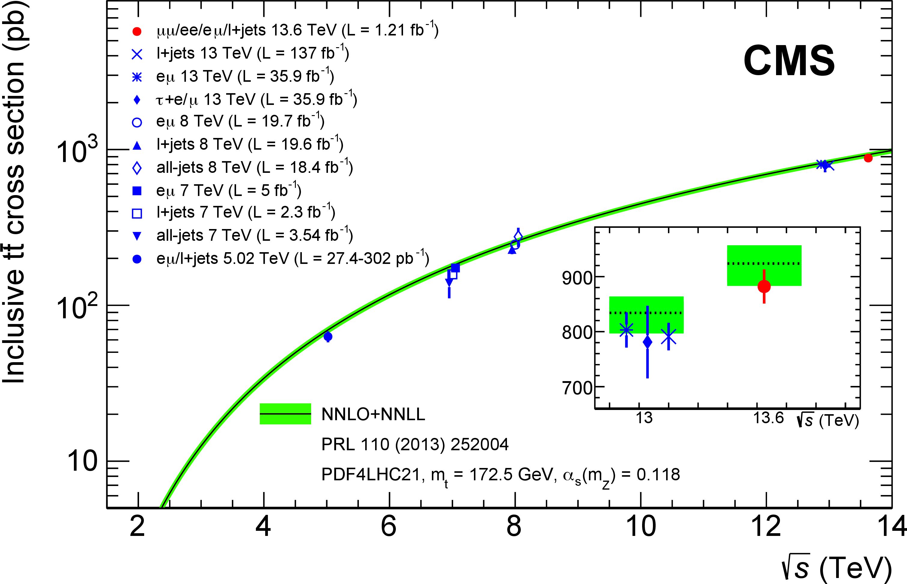
Figure 1:
Summary of CMS measurements of the $ \mathrm{t} \overline{\mathrm{t}} $ production cross section as a function of $ \sqrt{s} $ compared to the NNLO QCD calculation complemented with NNLL resummation (TOP++ v2.0 [77]). The theory band represents uncertainties due to the renormalisation and factorisation scales, parton distribution functions, and the strong coupling. The measurements and the theoretical calculation are quoted at $ m_{\mathrm{t}}= $ 172.5 GeV. Measurements made at the same $ \sqrt{s} $ are slightly offset for clarity. An enlarged inset is included to highlight the difference between 13 and 13.6 TeV predictions and results. Figure taken from Ref. [82]. |
png pdf |
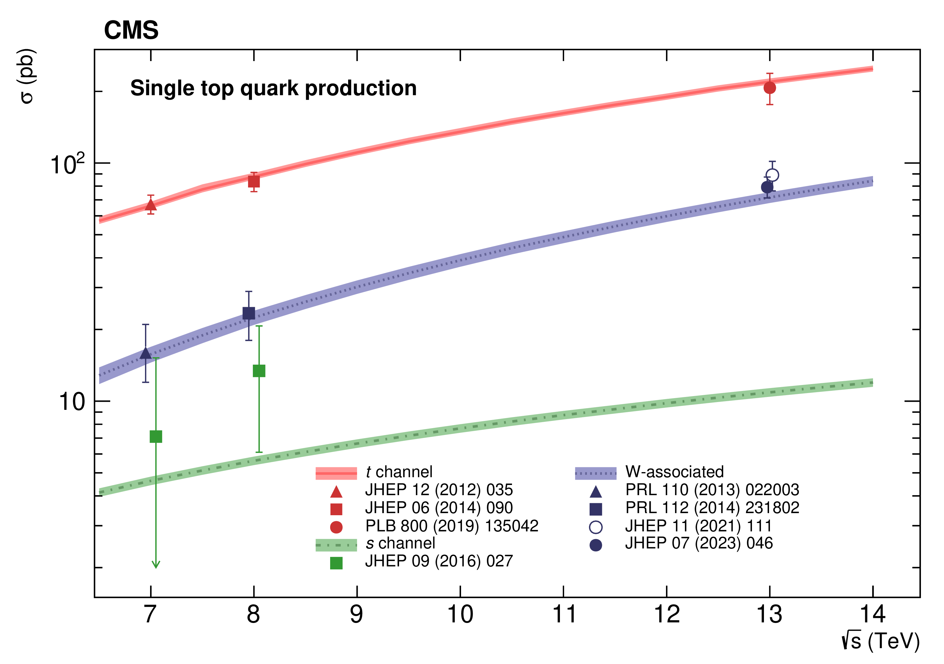
Figure 2:
Summary of single top quark production cross section measurements by CMS. Theoretical calculations for $ t $-channel, $ s $-channel, and W-associated production are courtesy of N. Kidonakis [88,89]. |
png pdf |
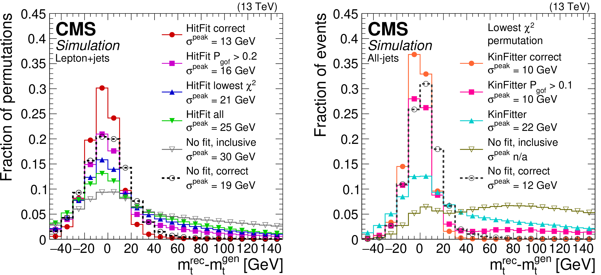
Figure 3:
Reconstructed top quark mass resolution with and without the HITFIT/KINFITTER kinematic reconstruction in the lepton+jets (left) and all-jets (right) channels. Multiple reconstruction options with and without kinematic fit are represented by lines of different colour, and ``correct'' denotes the correct parton-jet assignments as discussed in the text. The HITFIT/KINFITTER reconstruction with a cutoff on $ P_{\text{gof}} $ is used for measuring the top quark mass [61,62,62]. |
png pdf |
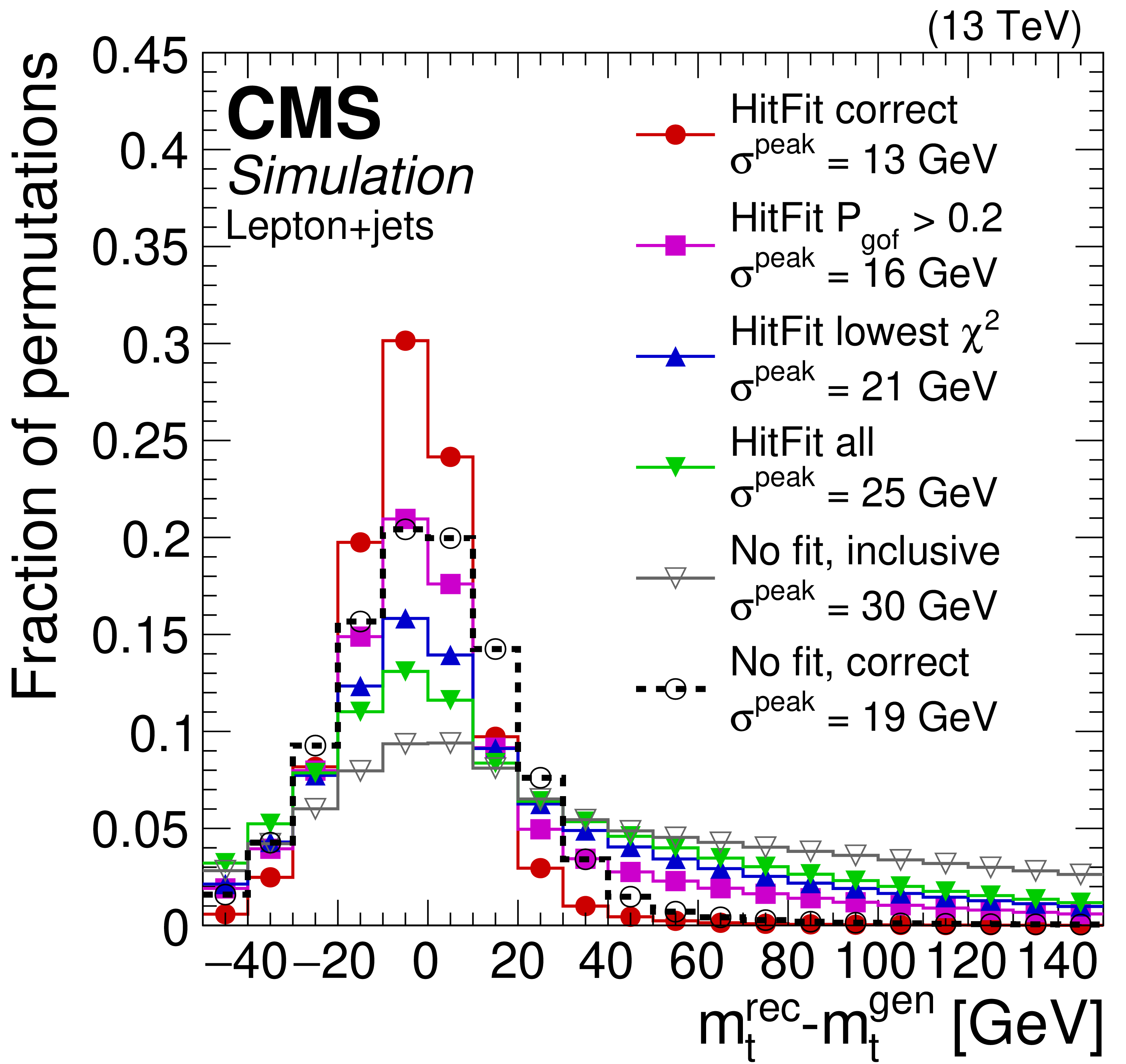
Figure 3-a:
Reconstructed top quark mass resolution with and without the HITFIT/KINFITTER kinematic reconstruction in the lepton+jets (left) and all-jets (right) channels. Multiple reconstruction options with and without kinematic fit are represented by lines of different colour, and ``correct'' denotes the correct parton-jet assignments as discussed in the text. The HITFIT/KINFITTER reconstruction with a cutoff on $ P_{\text{gof}} $ is used for measuring the top quark mass [61,62,62]. |

png pdf |
Figure 3-b:
Reconstructed top quark mass resolution with and without the HITFIT/KINFITTER kinematic reconstruction in the lepton+jets (left) and all-jets (right) channels. Multiple reconstruction options with and without kinematic fit are represented by lines of different colour, and ``correct'' denotes the correct parton-jet assignments as discussed in the text. The HITFIT/KINFITTER reconstruction with a cutoff on $ P_{\text{gof}} $ is used for measuring the top quark mass [61,62,62]. |
png pdf |
Figure 4:
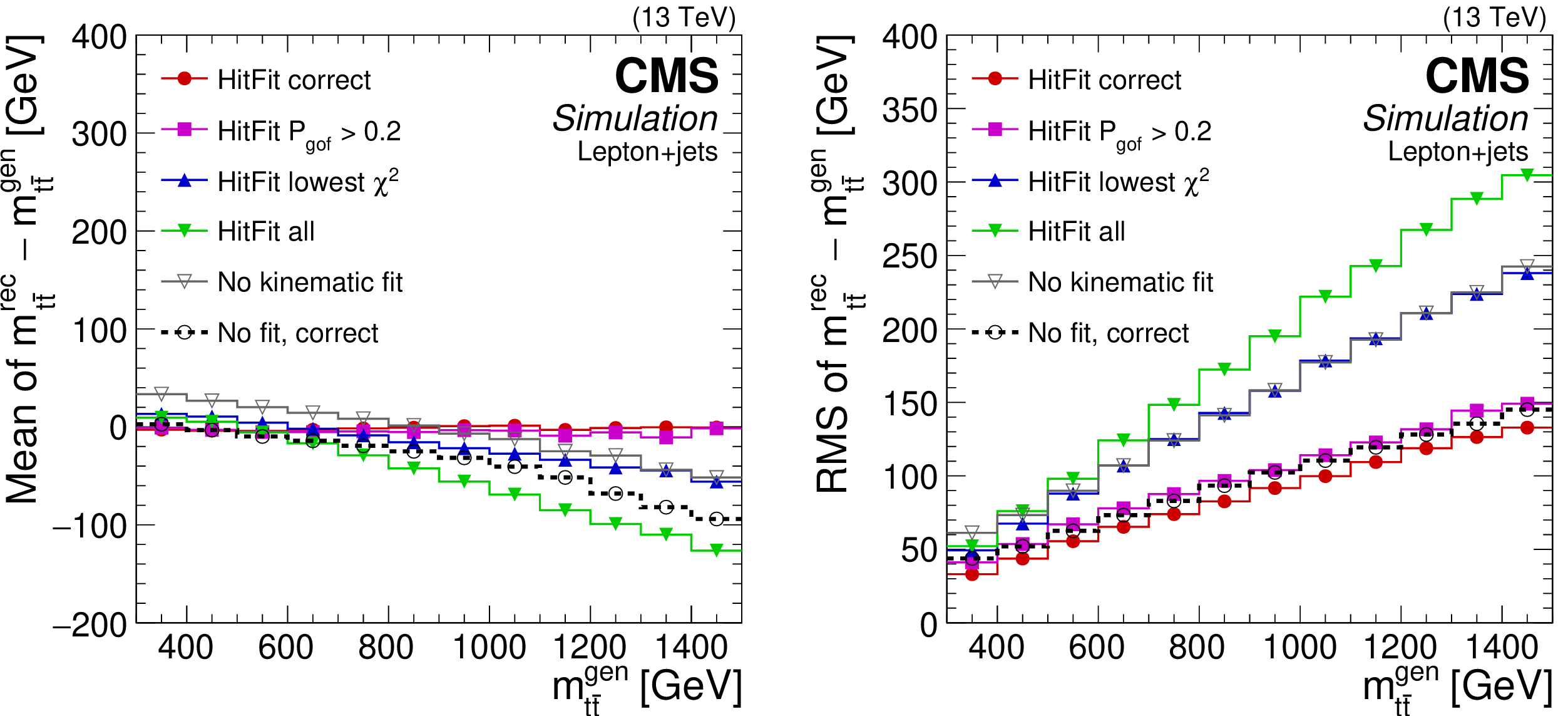
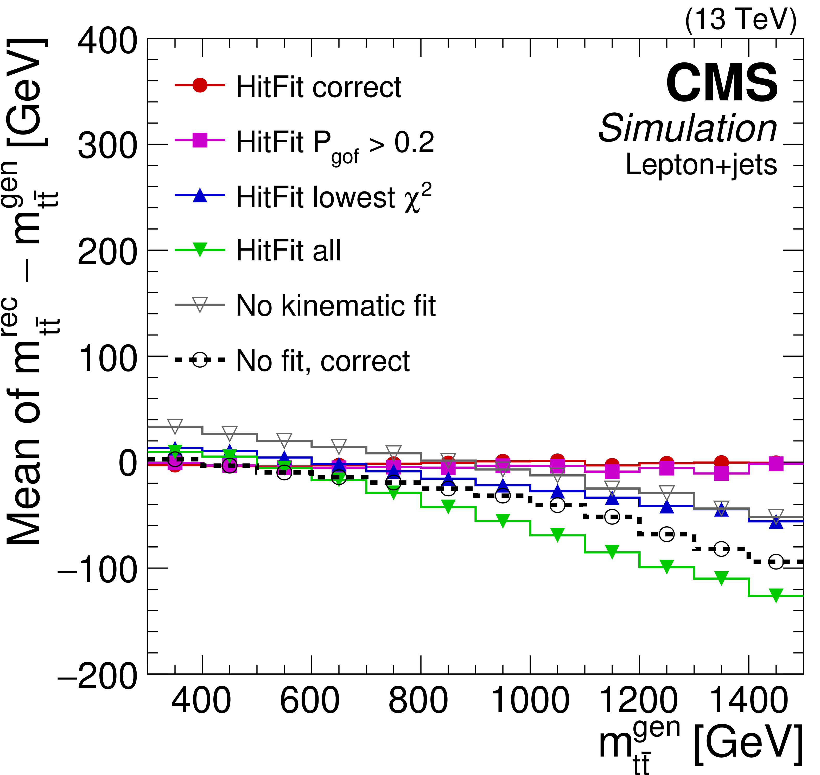
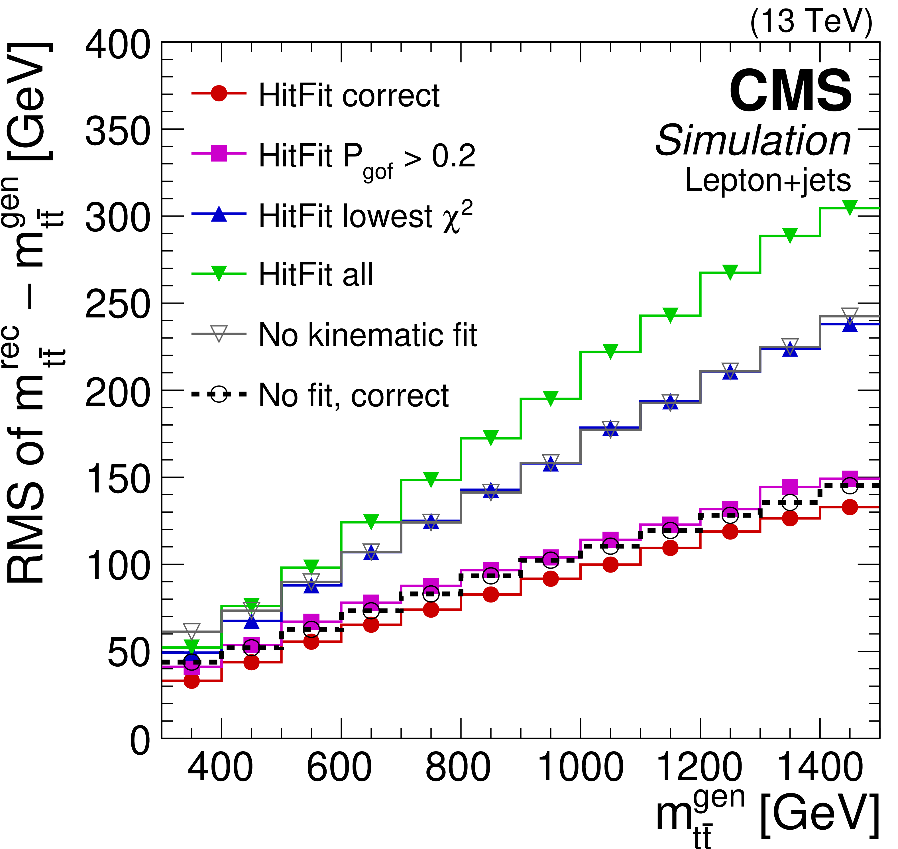
Reconstructed $ \mathrm{t} \overline{\mathrm{t}} $ mass bias (left) and resolution (right) with and without the HITFIT kinematic reconstruction in the lepton+jets channel, as functions of the $ \mathrm{t} \overline{\mathrm{t}} $ invariant mass at generator level. Multiple reconstruction options with and without kinematic fit are represented by lines of different colour, and ``correct'' denotes the correct parton-jet assignments as discussed in the text. The HITFIT reconstruction with a cutoff on $ P_{\text{gof}} $ is used for measuring the top quark mass [61]. |
png pdf |
Figure 4-a:
Reconstructed $ \mathrm{t} \overline{\mathrm{t}} $ mass bias (left) and resolution (right) with and without the HITFIT kinematic reconstruction in the lepton+jets channel, as functions of the $ \mathrm{t} \overline{\mathrm{t}} $ invariant mass at generator level. Multiple reconstruction options with and without kinematic fit are represented by lines of different colour, and ``correct'' denotes the correct parton-jet assignments as discussed in the text. The HITFIT reconstruction with a cutoff on $ P_{\text{gof}} $ is used for measuring the top quark mass [61]. |
png pdf |
Figure 4-b:
Reconstructed $ \mathrm{t} \overline{\mathrm{t}} $ mass bias (left) and resolution (right) with and without the HITFIT kinematic reconstruction in the lepton+jets channel, as functions of the $ \mathrm{t} \overline{\mathrm{t}} $ invariant mass at generator level. Multiple reconstruction options with and without kinematic fit are represented by lines of different colour, and ``correct'' denotes the correct parton-jet assignments as discussed in the text. The HITFIT reconstruction with a cutoff on $ P_{\text{gof}} $ is used for measuring the top quark mass [61]. |

png pdf |
Figure 5:
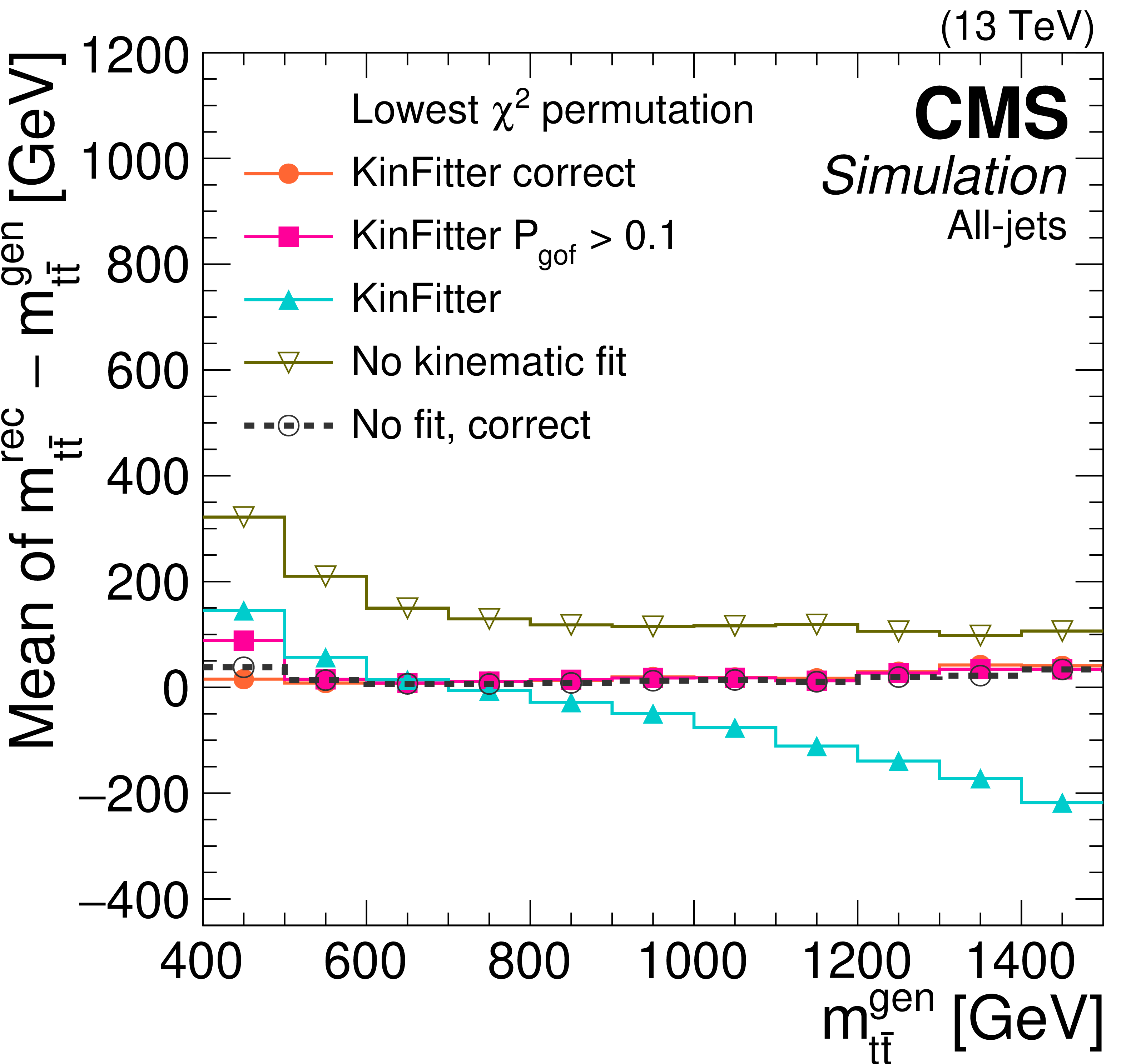
Reconstructed $ \mathrm{t} \overline{\mathrm{t}} $ mass bias (left) and resolution (right) with and without the KINFITTER kinematic reconstruction in the all-jet channel, as functions of the $ \mathrm{t} \overline{\mathrm{t}} $ invariant mass at generator level. Multiple reconstruction options with and without kinematic fit are represented by lines of different colour, and ``correct'' denotes the correct parton-jet assignments as discussed in the text. The KINFITTER reconstruction with a cutoff on $ P_{\text{gof}} $ is used for measuring the top quark mass [62]. |
png pdf |
Figure 5-a:
Reconstructed $ \mathrm{t} \overline{\mathrm{t}} $ mass bias (left) and resolution (right) with and without the KINFITTER kinematic reconstruction in the all-jet channel, as functions of the $ \mathrm{t} \overline{\mathrm{t}} $ invariant mass at generator level. Multiple reconstruction options with and without kinematic fit are represented by lines of different colour, and ``correct'' denotes the correct parton-jet assignments as discussed in the text. The KINFITTER reconstruction with a cutoff on $ P_{\text{gof}} $ is used for measuring the top quark mass [62]. |

png pdf |
Figure 5-b:
Reconstructed $ \mathrm{t} \overline{\mathrm{t}} $ mass bias (left) and resolution (right) with and without the KINFITTER kinematic reconstruction in the all-jet channel, as functions of the $ \mathrm{t} \overline{\mathrm{t}} $ invariant mass at generator level. Multiple reconstruction options with and without kinematic fit are represented by lines of different colour, and ``correct'' denotes the correct parton-jet assignments as discussed in the text. The KINFITTER reconstruction with a cutoff on $ P_{\text{gof}} $ is used for measuring the top quark mass [62]. |

png pdf |
Figure 6:
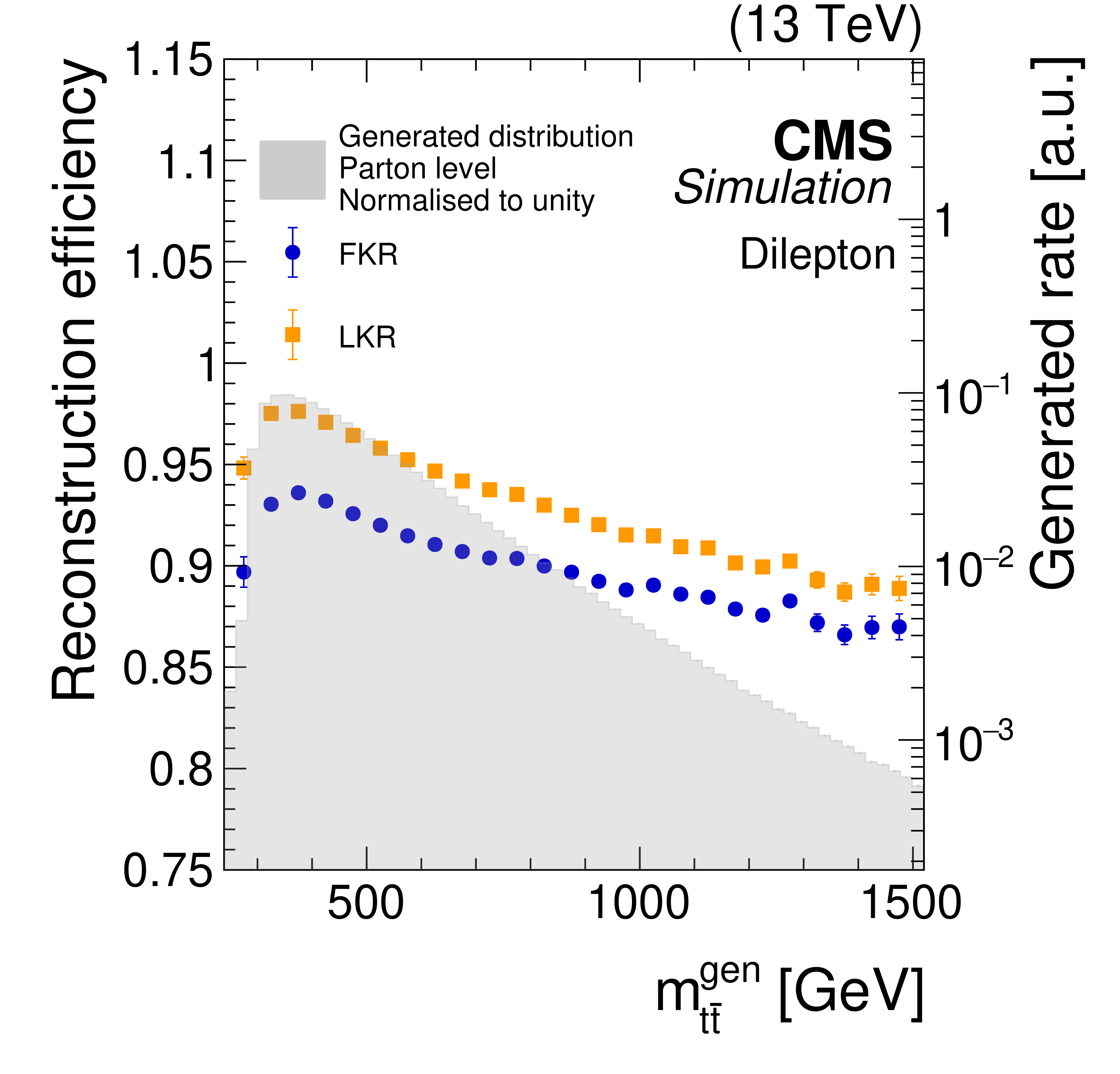
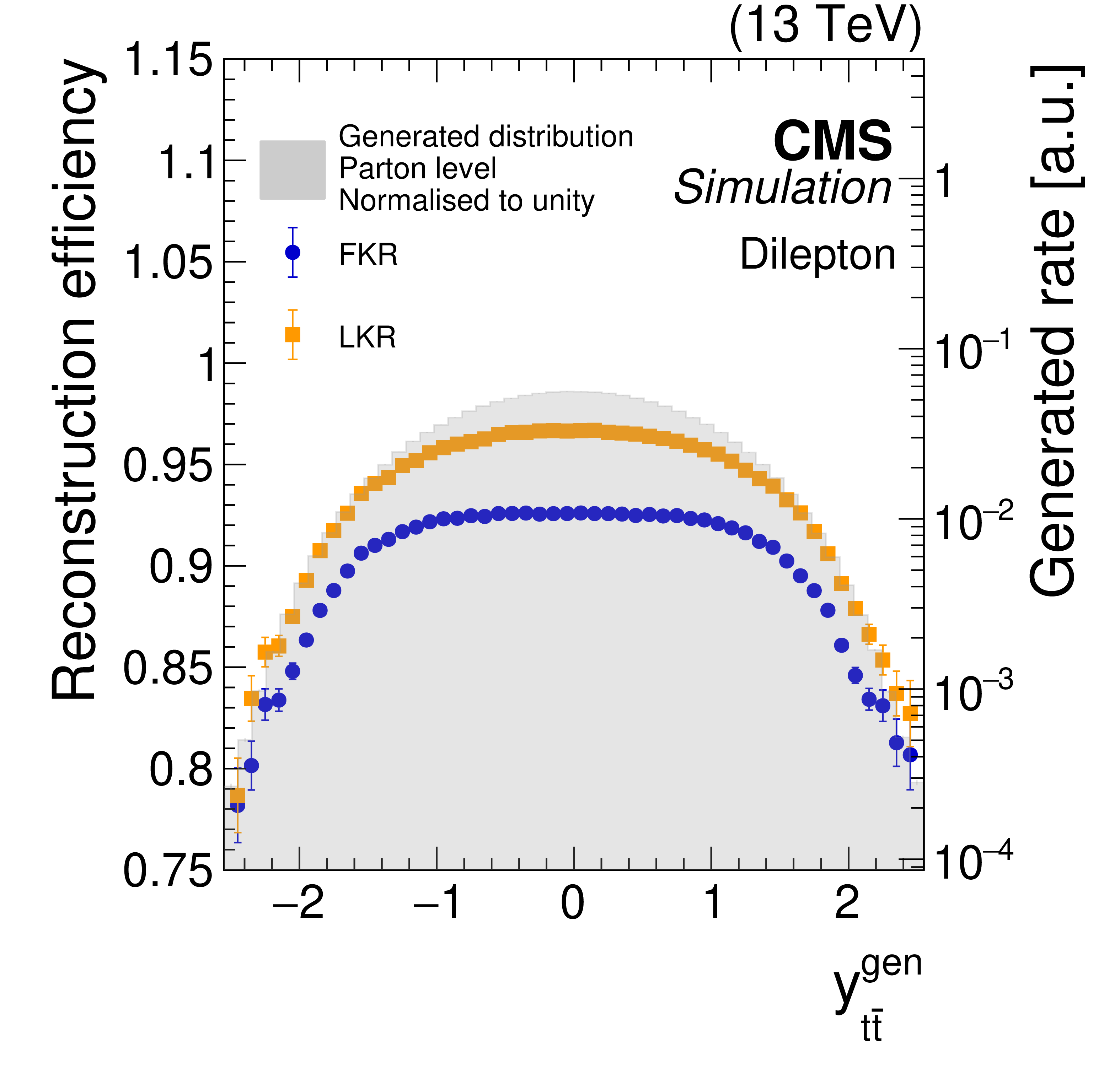
The reconstruction efficiencies for the full kinematic reconstruction (FKR, blue circles) and loose kinematic reconstruction (LKR, orange squares) are shown as functions of the invariant mass, transverse momentum, and rapidity of the reconstructed $ \mathrm{t} \overline{\mathrm{t}} $ system. The averaged efficiencies are 92 (96)% for the FKR (LKR). The corresponding parton-generator-level distributions, normalised to unit area, for $ \mathrm{t} \overline{\mathrm{t}} $ production are represented by the grey shaded areas, shown on the logarithmic scale (right $ y $ axis). The POWHEG+PYTHIA-8 $ \mathrm{t} \overline{\mathrm{t}} $ simulated samples are used. |
png pdf |
Figure 6-a:
The reconstruction efficiencies for the full kinematic reconstruction (FKR, blue circles) and loose kinematic reconstruction (LKR, orange squares) are shown as functions of the invariant mass, transverse momentum, and rapidity of the reconstructed $ \mathrm{t} \overline{\mathrm{t}} $ system. The averaged efficiencies are 92 (96)% for the FKR (LKR). The corresponding parton-generator-level distributions, normalised to unit area, for $ \mathrm{t} \overline{\mathrm{t}} $ production are represented by the grey shaded areas, shown on the logarithmic scale (right $ y $ axis). The POWHEG+PYTHIA-8 $ \mathrm{t} \overline{\mathrm{t}} $ simulated samples are used. |

png pdf |
Figure 6-b:
The reconstruction efficiencies for the full kinematic reconstruction (FKR, blue circles) and loose kinematic reconstruction (LKR, orange squares) are shown as functions of the invariant mass, transverse momentum, and rapidity of the reconstructed $ \mathrm{t} \overline{\mathrm{t}} $ system. The averaged efficiencies are 92 (96)% for the FKR (LKR). The corresponding parton-generator-level distributions, normalised to unit area, for $ \mathrm{t} \overline{\mathrm{t}} $ production are represented by the grey shaded areas, shown on the logarithmic scale (right $ y $ axis). The POWHEG+PYTHIA-8 $ \mathrm{t} \overline{\mathrm{t}} $ simulated samples are used. |
png pdf |
Figure 6-c:
The reconstruction efficiencies for the full kinematic reconstruction (FKR, blue circles) and loose kinematic reconstruction (LKR, orange squares) are shown as functions of the invariant mass, transverse momentum, and rapidity of the reconstructed $ \mathrm{t} \overline{\mathrm{t}} $ system. The averaged efficiencies are 92 (96)% for the FKR (LKR). The corresponding parton-generator-level distributions, normalised to unit area, for $ \mathrm{t} \overline{\mathrm{t}} $ production are represented by the grey shaded areas, shown on the logarithmic scale (right $ y $ axis). The POWHEG+PYTHIA-8 $ \mathrm{t} \overline{\mathrm{t}} $ simulated samples are used. |
png pdf |
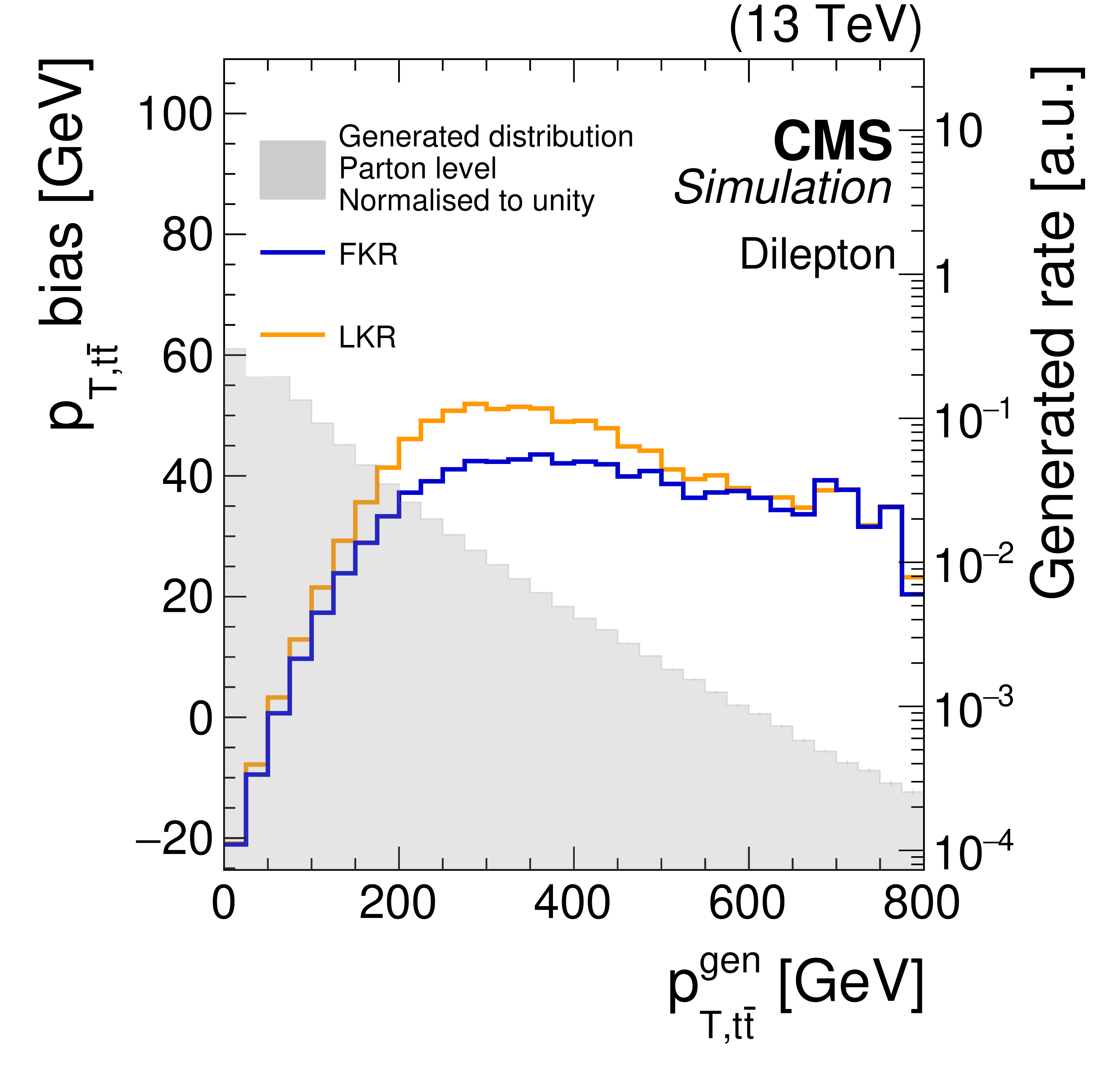
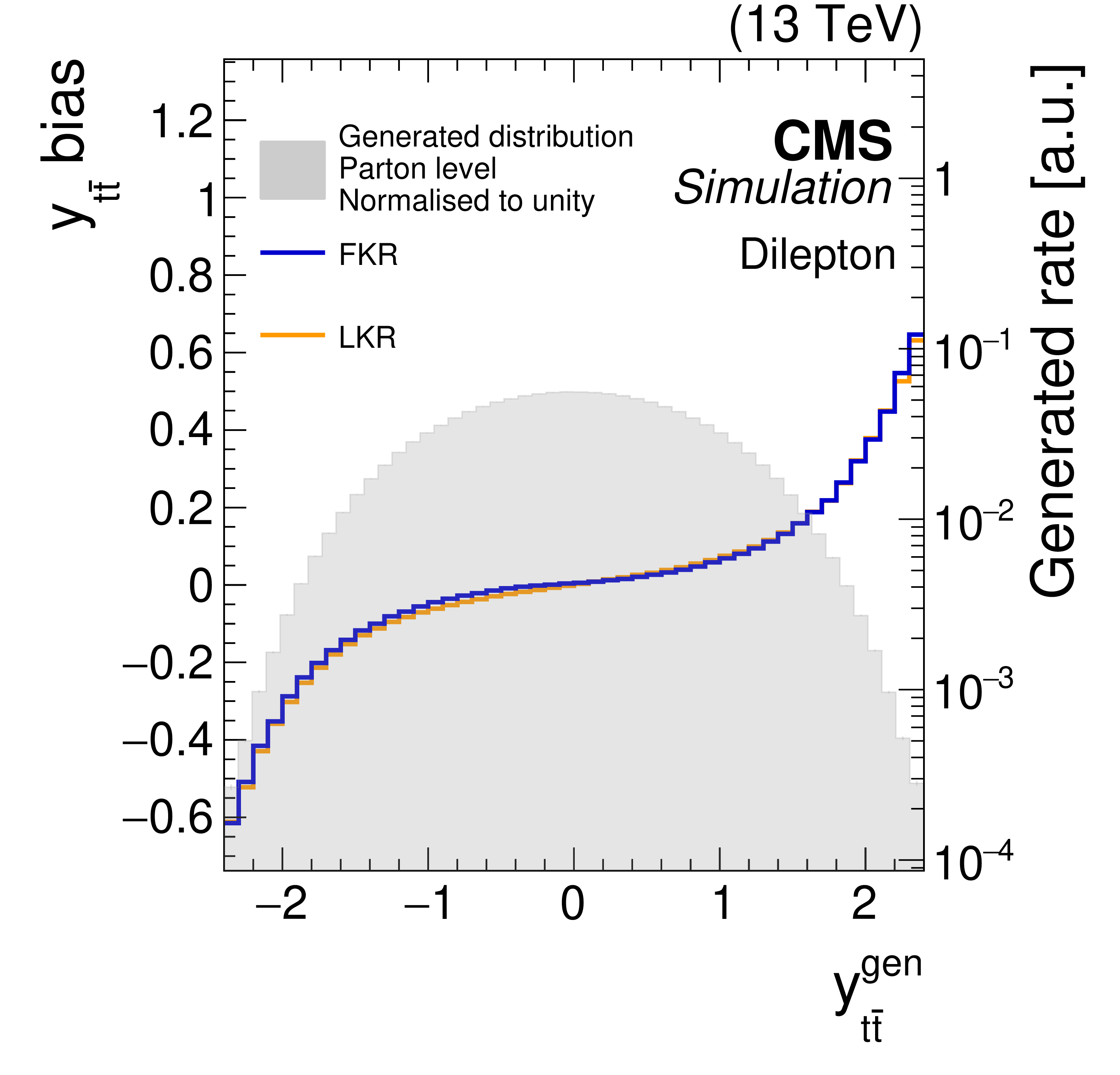
Figure 7:
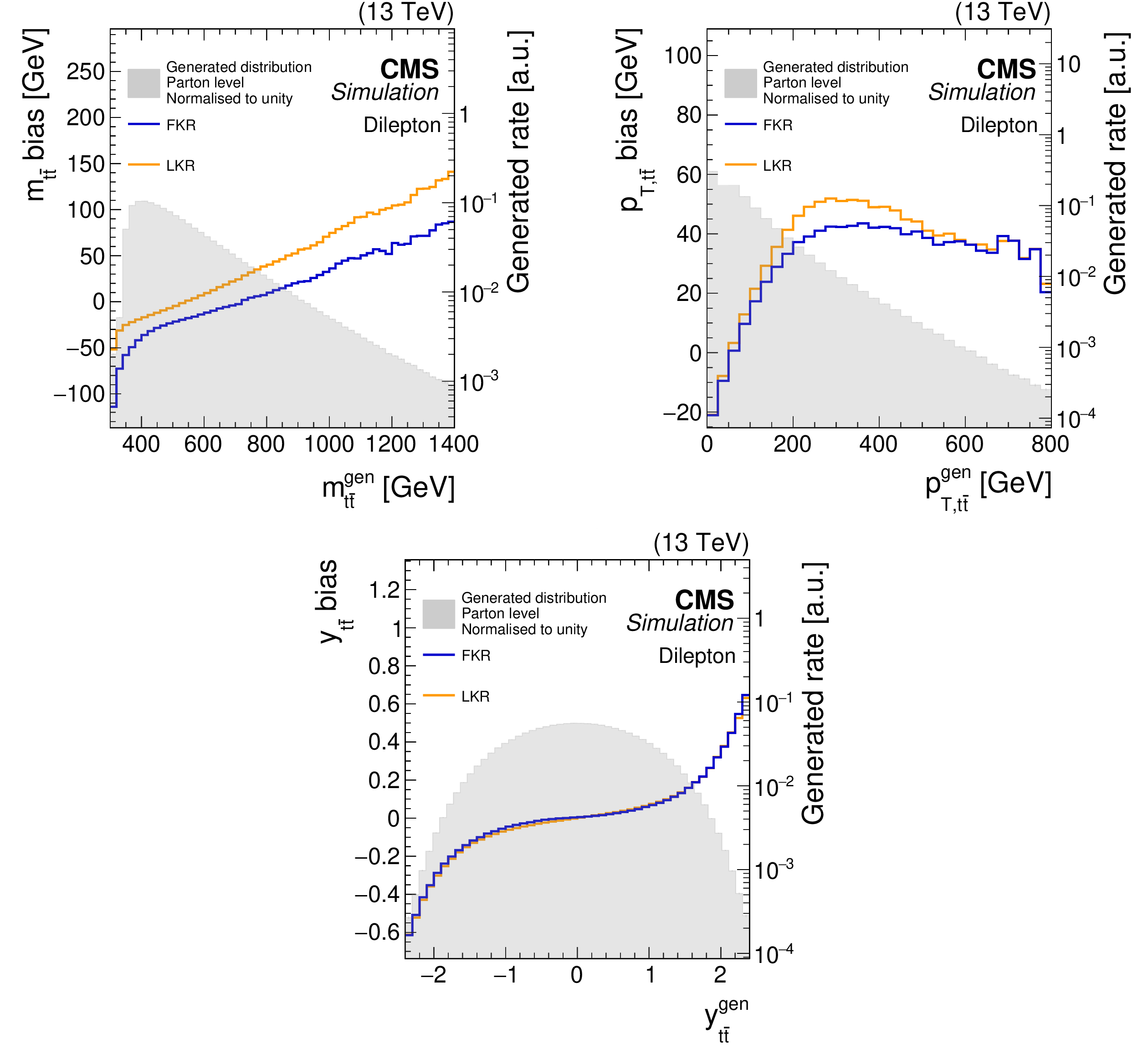
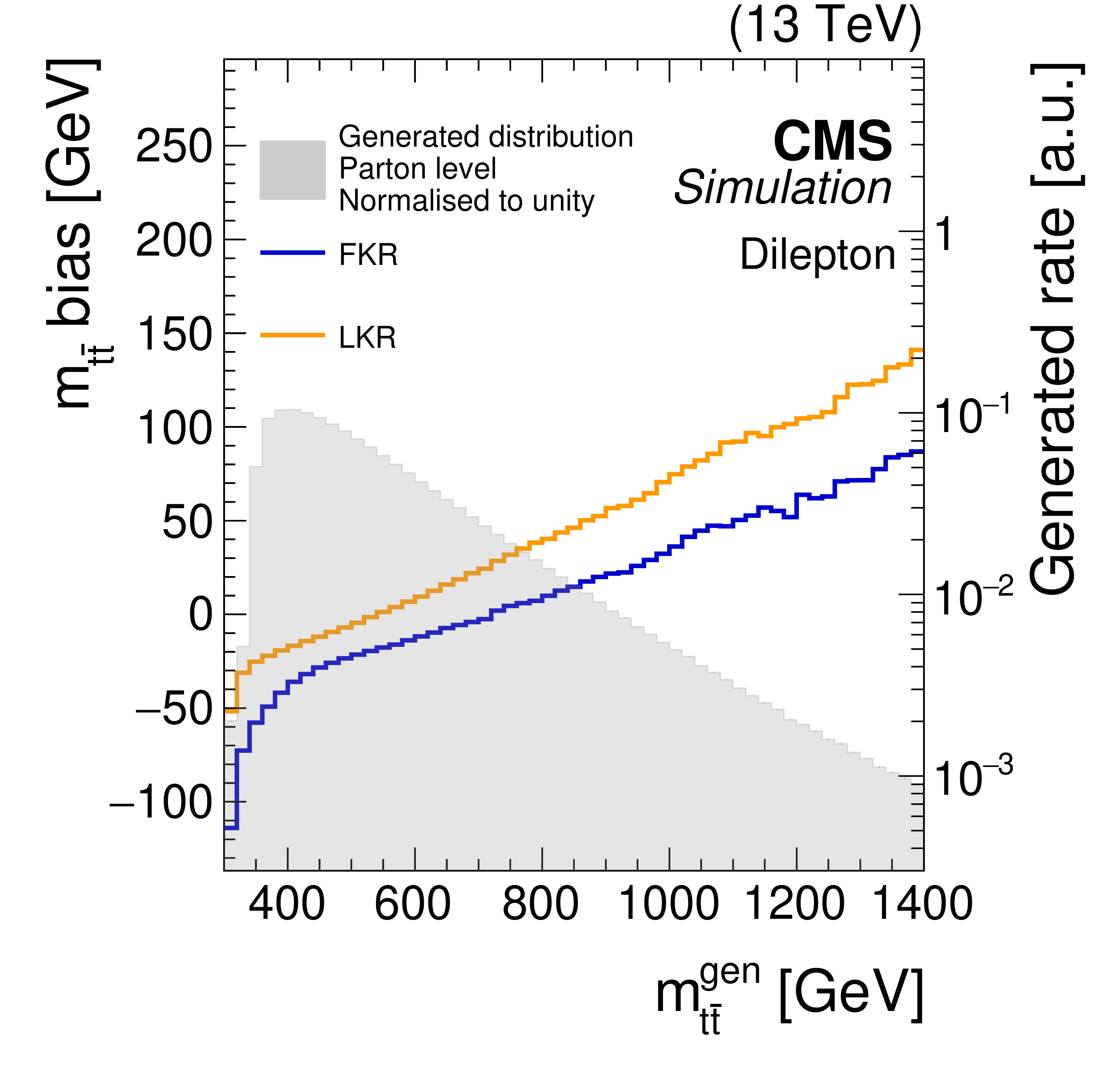
The biases (solid lines), as defined in the text, for the full kinematic reconstruction (FKR, blue) and loose kinematic reconstruction (LKR, orange) are shown for the invariant mass, transverse momentum, and rapidity of the $ \mathrm{t} \overline{\mathrm{t}} $ system, as a function of the same variables at the generator level. The corresponding parton-generator-level distributions, normalised to unit area, for $ \mathrm{t} \overline{\mathrm{t}} $ production are represented by the grey shaded areas, shown on the logarithmic scale (right $ y $ axis). The POWHEG+PYTHIA-8 $ \mathrm{t} \overline{\mathrm{t}} $ simulated samples are used. |
png pdf |
Figure 7-a:
The biases (solid lines), as defined in the text, for the full kinematic reconstruction (FKR, blue) and loose kinematic reconstruction (LKR, orange) are shown for the invariant mass, transverse momentum, and rapidity of the $ \mathrm{t} \overline{\mathrm{t}} $ system, as a function of the same variables at the generator level. The corresponding parton-generator-level distributions, normalised to unit area, for $ \mathrm{t} \overline{\mathrm{t}} $ production are represented by the grey shaded areas, shown on the logarithmic scale (right $ y $ axis). The POWHEG+PYTHIA-8 $ \mathrm{t} \overline{\mathrm{t}} $ simulated samples are used. |
png pdf |
Figure 7-b:
The biases (solid lines), as defined in the text, for the full kinematic reconstruction (FKR, blue) and loose kinematic reconstruction (LKR, orange) are shown for the invariant mass, transverse momentum, and rapidity of the $ \mathrm{t} \overline{\mathrm{t}} $ system, as a function of the same variables at the generator level. The corresponding parton-generator-level distributions, normalised to unit area, for $ \mathrm{t} \overline{\mathrm{t}} $ production are represented by the grey shaded areas, shown on the logarithmic scale (right $ y $ axis). The POWHEG+PYTHIA-8 $ \mathrm{t} \overline{\mathrm{t}} $ simulated samples are used. |
png pdf |
Figure 7-c:
The biases (solid lines), as defined in the text, for the full kinematic reconstruction (FKR, blue) and loose kinematic reconstruction (LKR, orange) are shown for the invariant mass, transverse momentum, and rapidity of the $ \mathrm{t} \overline{\mathrm{t}} $ system, as a function of the same variables at the generator level. The corresponding parton-generator-level distributions, normalised to unit area, for $ \mathrm{t} \overline{\mathrm{t}} $ production are represented by the grey shaded areas, shown on the logarithmic scale (right $ y $ axis). The POWHEG+PYTHIA-8 $ \mathrm{t} \overline{\mathrm{t}} $ simulated samples are used. |

png pdf |
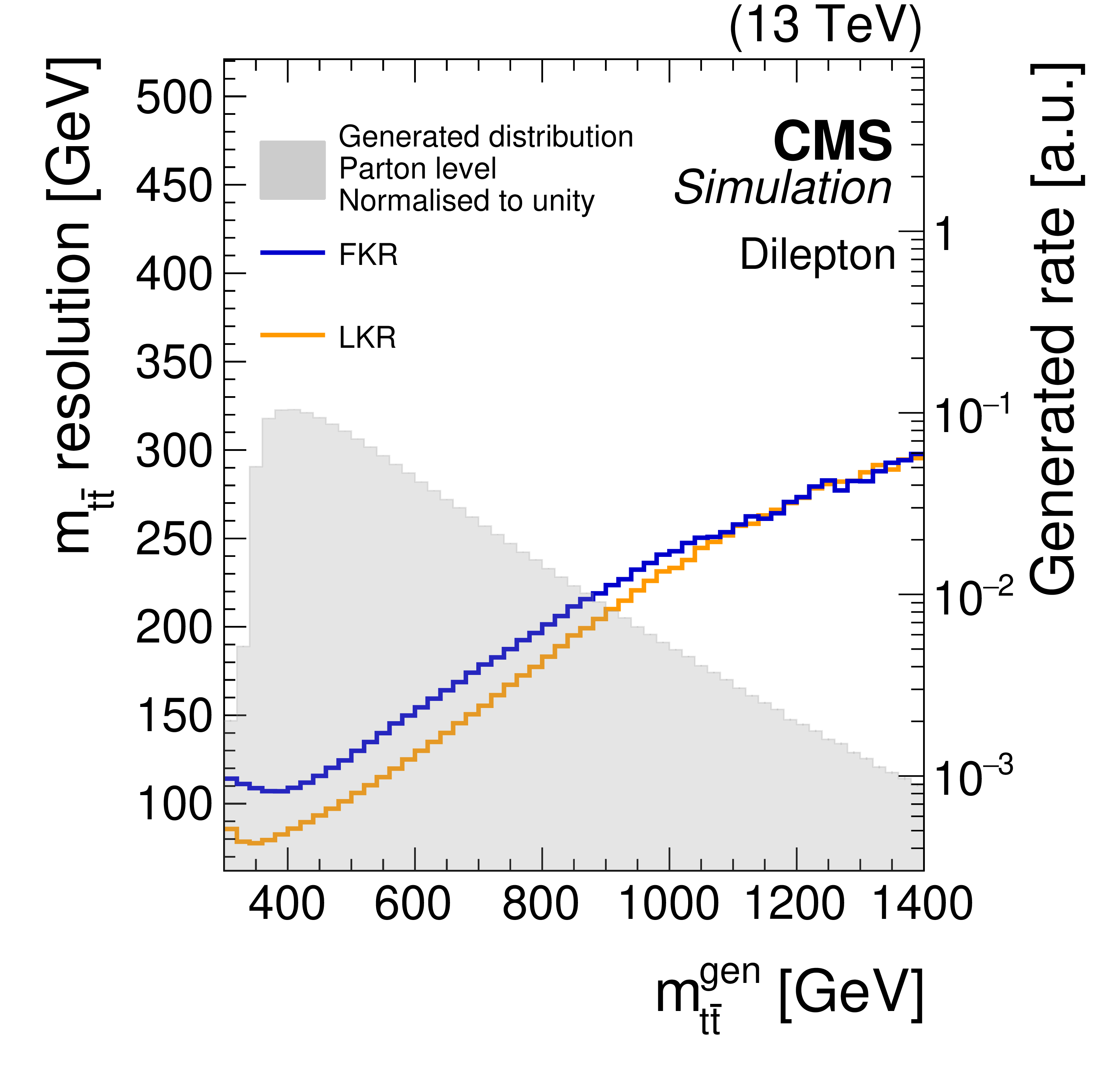
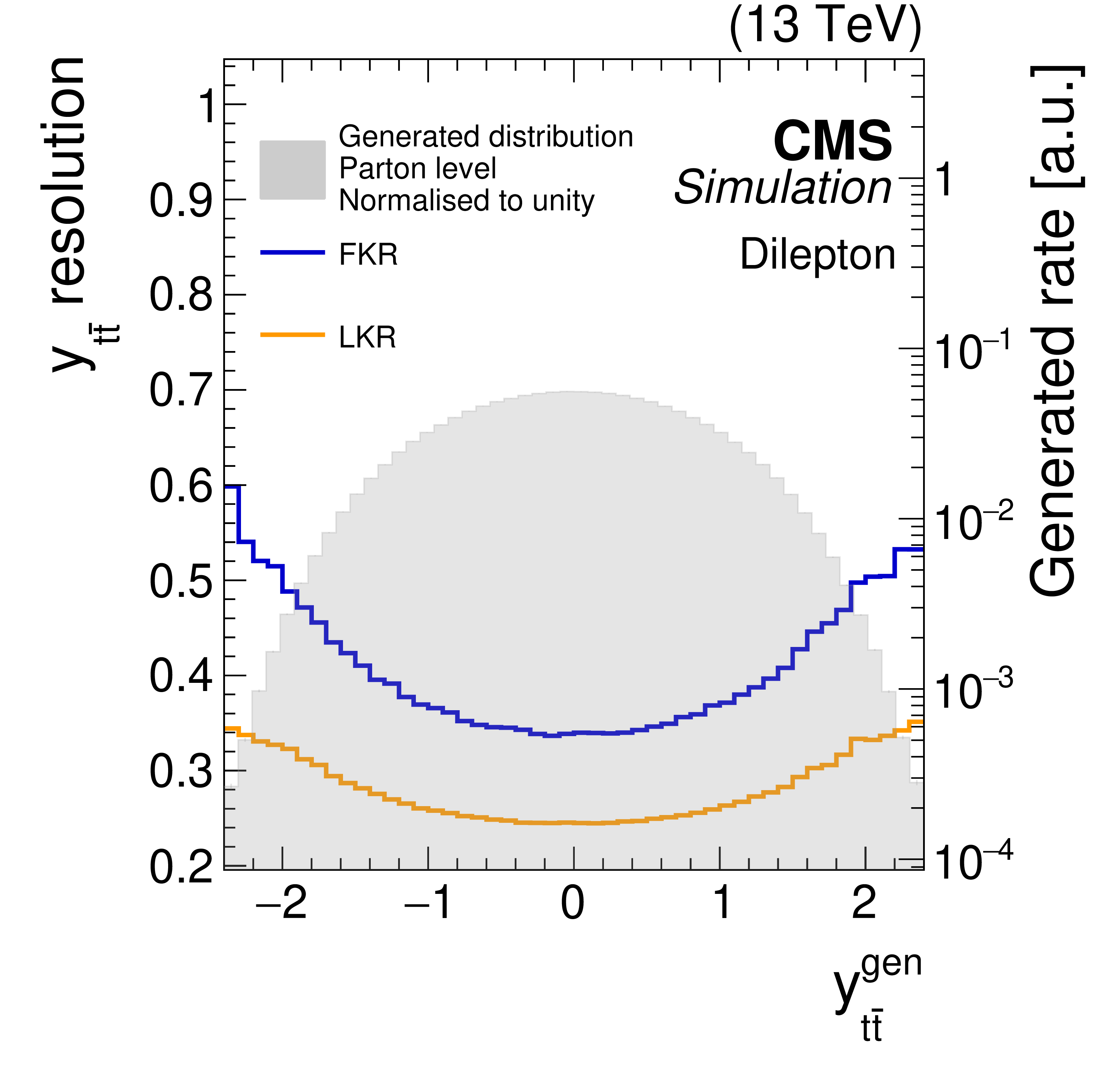
Figure 8:
The resolutions (solid lines), as defined in the text, for the full kinematic reconstruction (FKR, blue) and loose kinematic reconstruction (LKR, orange) are shown as functions of the invariant mass, transverse momentum, and rapidity of the $ \mathrm{t} \overline{\mathrm{t}} $ system at the generator level. The corresponding parton-generator-level distributions, normalised to unit area, for $ \mathrm{t} \overline{\mathrm{t}} $ production are represented by the grey shaded areas, shown on the logarithmic scale (right $ y $ axis). The POWHEG+PYTHIA-8 $ \mathrm{t} \overline{\mathrm{t}} $ simulated samples are used. |
png pdf |
Figure 8-a:
The resolutions (solid lines), as defined in the text, for the full kinematic reconstruction (FKR, blue) and loose kinematic reconstruction (LKR, orange) are shown as functions of the invariant mass, transverse momentum, and rapidity of the $ \mathrm{t} \overline{\mathrm{t}} $ system at the generator level. The corresponding parton-generator-level distributions, normalised to unit area, for $ \mathrm{t} \overline{\mathrm{t}} $ production are represented by the grey shaded areas, shown on the logarithmic scale (right $ y $ axis). The POWHEG+PYTHIA-8 $ \mathrm{t} \overline{\mathrm{t}} $ simulated samples are used. |

png pdf |
Figure 8-b:
The resolutions (solid lines), as defined in the text, for the full kinematic reconstruction (FKR, blue) and loose kinematic reconstruction (LKR, orange) are shown as functions of the invariant mass, transverse momentum, and rapidity of the $ \mathrm{t} \overline{\mathrm{t}} $ system at the generator level. The corresponding parton-generator-level distributions, normalised to unit area, for $ \mathrm{t} \overline{\mathrm{t}} $ production are represented by the grey shaded areas, shown on the logarithmic scale (right $ y $ axis). The POWHEG+PYTHIA-8 $ \mathrm{t} \overline{\mathrm{t}} $ simulated samples are used. |
png pdf |
Figure 8-c:
The resolutions (solid lines), as defined in the text, for the full kinematic reconstruction (FKR, blue) and loose kinematic reconstruction (LKR, orange) are shown as functions of the invariant mass, transverse momentum, and rapidity of the $ \mathrm{t} \overline{\mathrm{t}} $ system at the generator level. The corresponding parton-generator-level distributions, normalised to unit area, for $ \mathrm{t} \overline{\mathrm{t}} $ production are represented by the grey shaded areas, shown on the logarithmic scale (right $ y $ axis). The POWHEG+PYTHIA-8 $ \mathrm{t} \overline{\mathrm{t}} $ simulated samples are used. |
png pdf |
Figure 9:
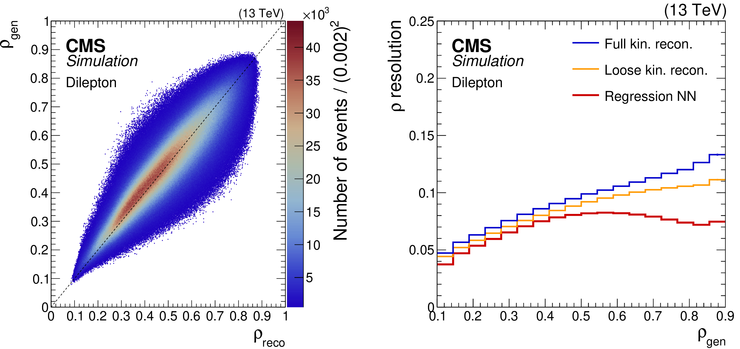
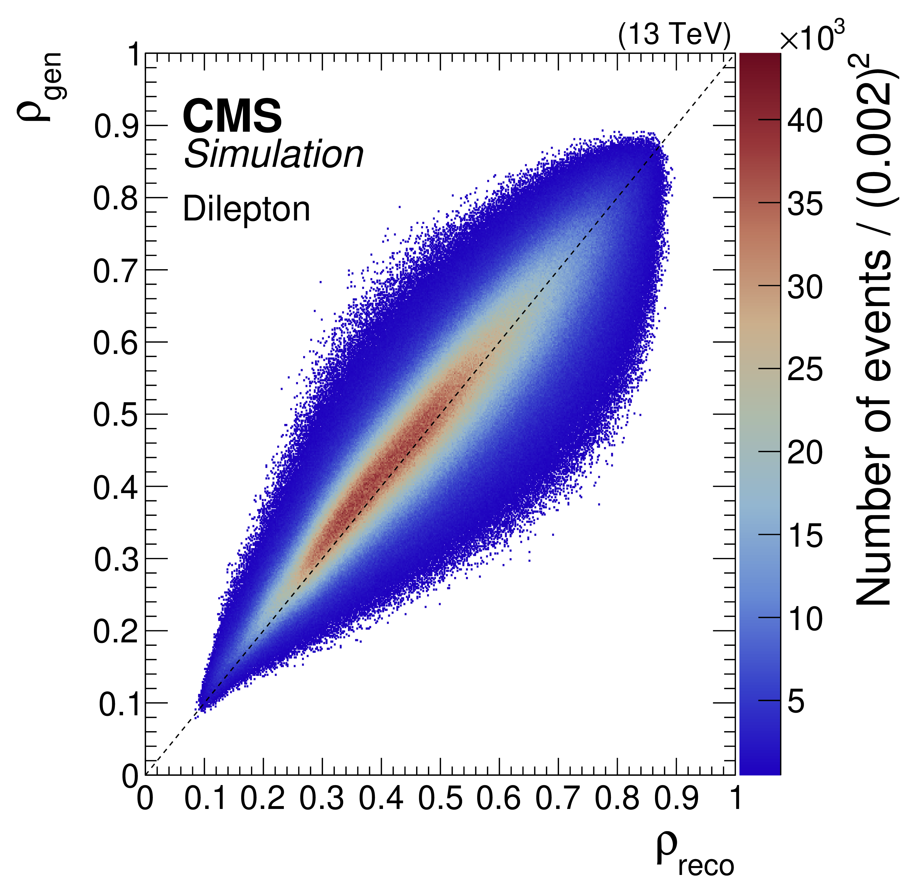
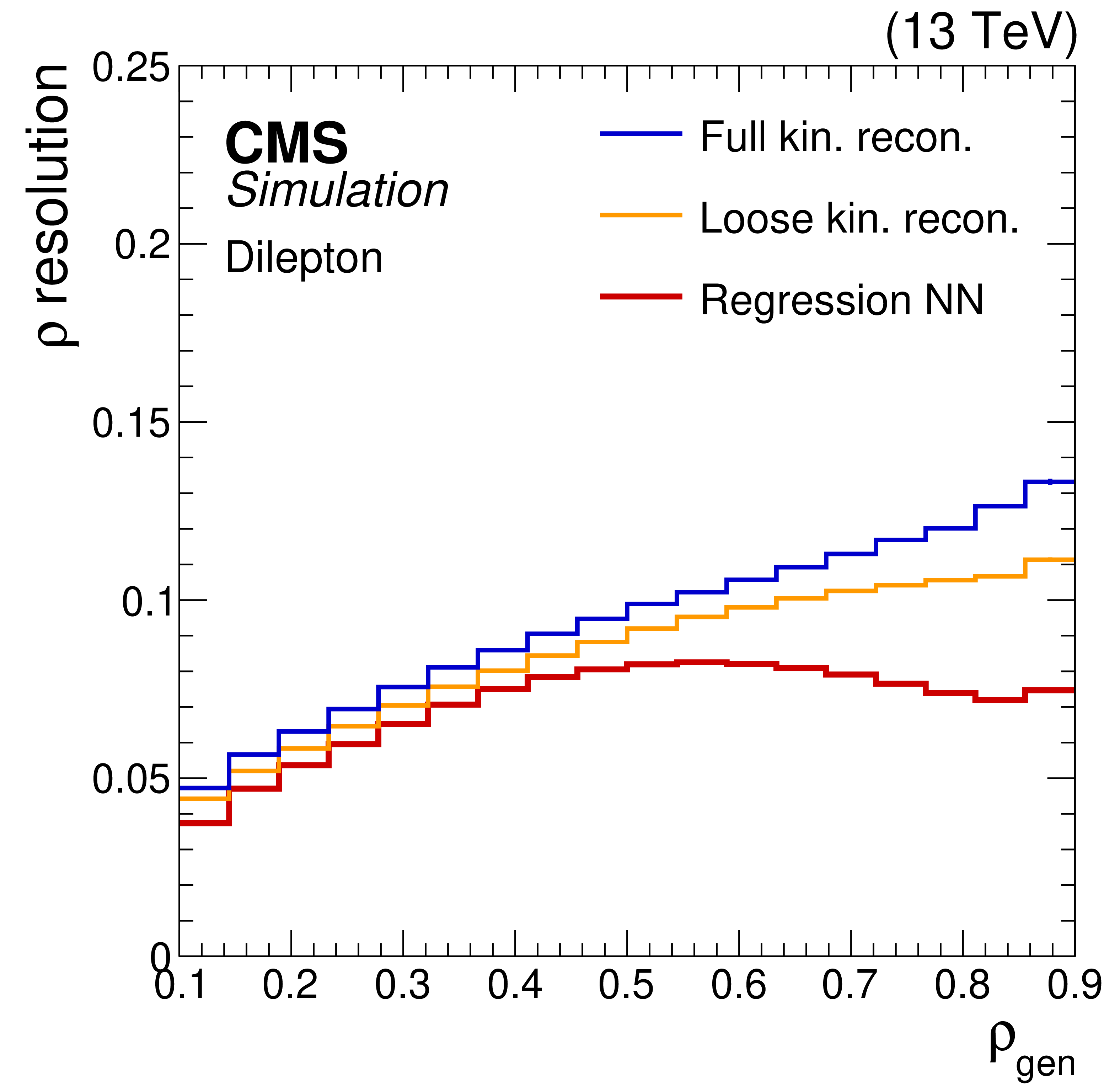
The correlation between $ \rho_{\text{gen}} $ and $ \rho_{\text{reco}} $ is shown for the regression NN reconstruction method (left). The $ \rho_{\text{reco}} $ resolution, defined in the text, as a function of $ \rho_{\text{gen}} $ (right) for the full (blue line) and loose (orange line) kinematic reconstructions and the regression NN (red line) methods. The number of events per bin in the left plot is shown by the colour scale. Figure taken from Ref. [69]. |
png pdf |
Figure 9-a:
The correlation between $ \rho_{\text{gen}} $ and $ \rho_{\text{reco}} $ is shown for the regression NN reconstruction method (left). The $ \rho_{\text{reco}} $ resolution, defined in the text, as a function of $ \rho_{\text{gen}} $ (right) for the full (blue line) and loose (orange line) kinematic reconstructions and the regression NN (red line) methods. The number of events per bin in the left plot is shown by the colour scale. Figure taken from Ref. [69]. |
png pdf |
Figure 9-b:
The correlation between $ \rho_{\text{gen}} $ and $ \rho_{\text{reco}} $ is shown for the regression NN reconstruction method (left). The $ \rho_{\text{reco}} $ resolution, defined in the text, as a function of $ \rho_{\text{gen}} $ (right) for the full (blue line) and loose (orange line) kinematic reconstructions and the regression NN (red line) methods. The number of events per bin in the left plot is shown by the colour scale. Figure taken from Ref. [69]. |
png pdf |
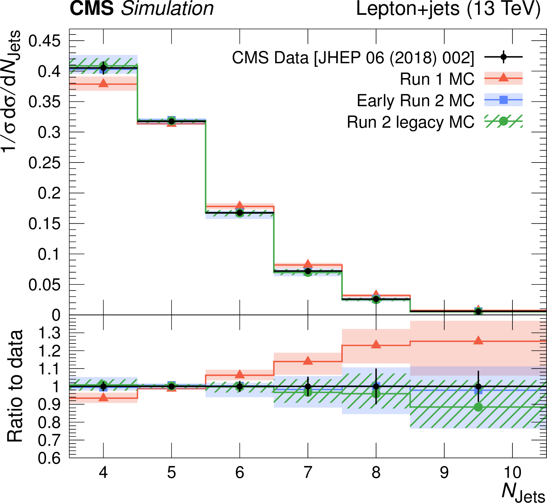
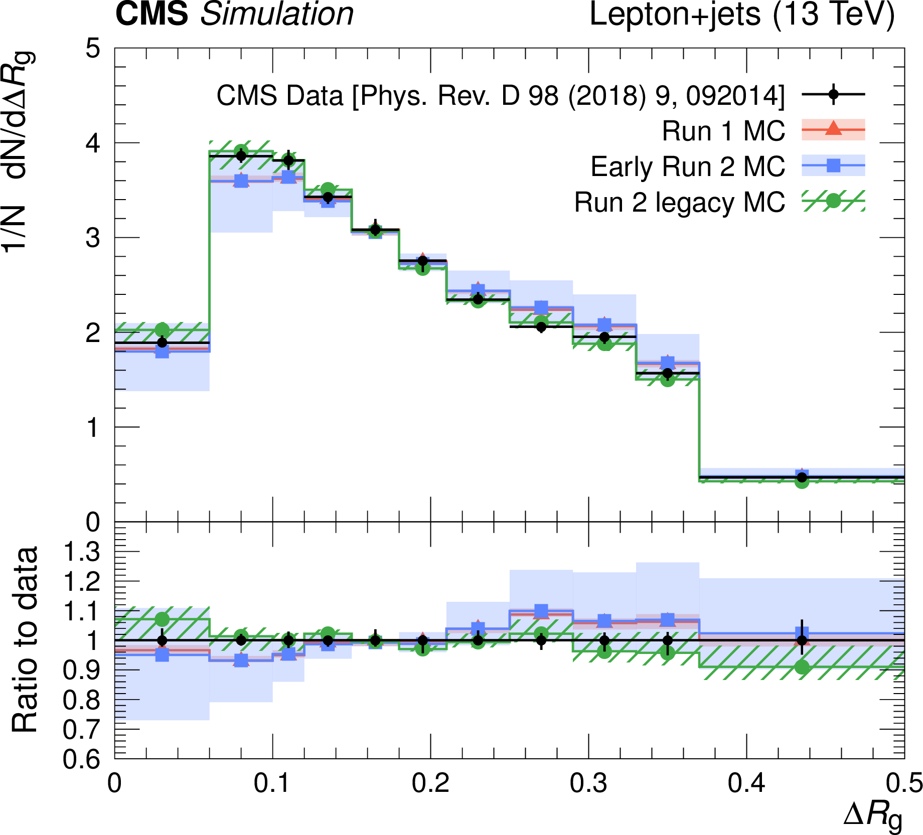
Figure 10:
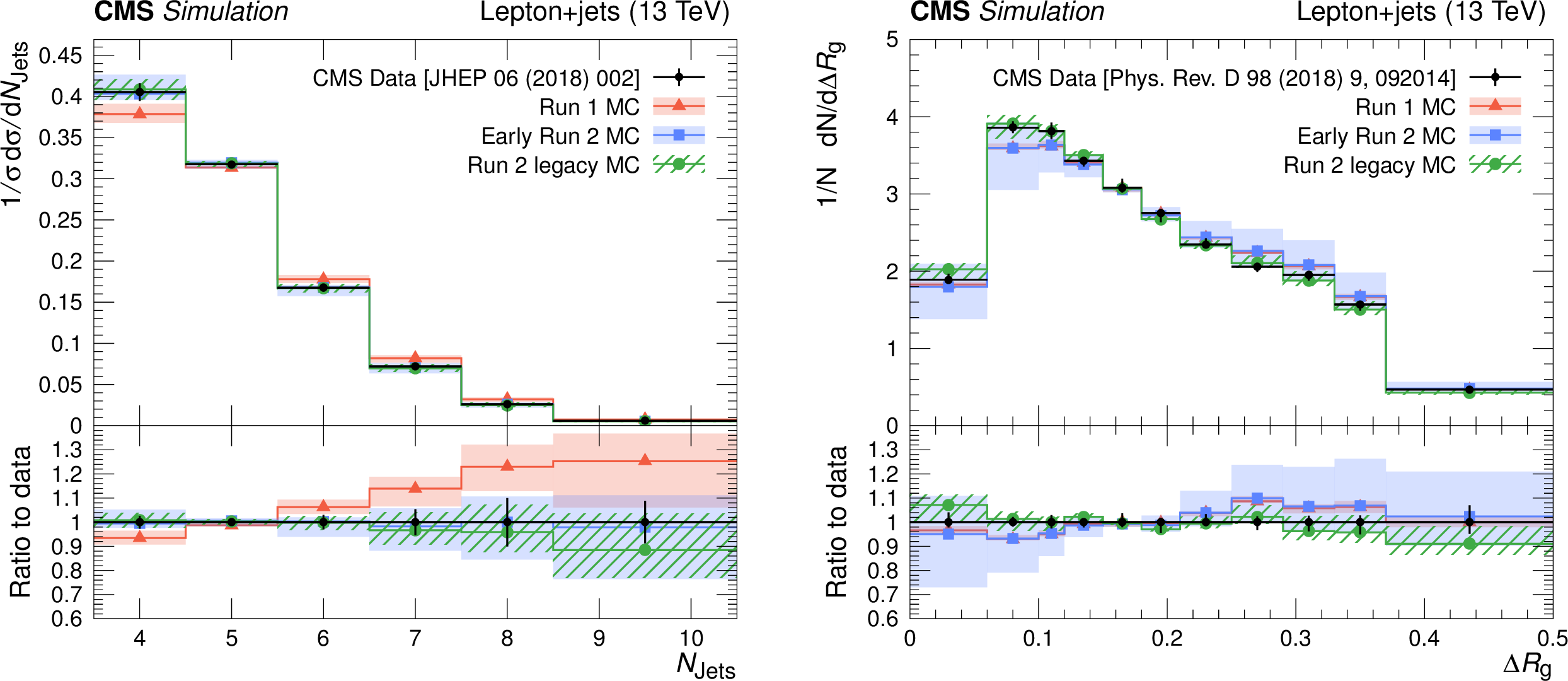
Distributions of the jet multiplicity $ N_{\text{Jets}} $ [134] (left) and the jet substructure observable $ \Delta R_{\mathrm{g}} $, the angle between the groomed subjets, normalised to the number of jets [135] (right) in $ \mathrm{t} \overline{\mathrm{t}} $ events at 13 TeV (black symbols). The data are compared to the MC simulation setups used in Run-1, early Run-2, and Run-2 legacy analyses, presented by bands of different style and colour. The uncertainty bands include ME scale, ME-PS matching, ISR, and FSR uncertainties. |
png pdf |
Figure 10-a:
Distributions of the jet multiplicity $ N_{\text{Jets}} $ [134] (left) and the jet substructure observable $ \Delta R_{\mathrm{g}} $, the angle between the groomed subjets, normalised to the number of jets [135] (right) in $ \mathrm{t} \overline{\mathrm{t}} $ events at 13 TeV (black symbols). The data are compared to the MC simulation setups used in Run-1, early Run-2, and Run-2 legacy analyses, presented by bands of different style and colour. The uncertainty bands include ME scale, ME-PS matching, ISR, and FSR uncertainties. |
png pdf |
Figure 10-b:
Distributions of the jet multiplicity $ N_{\text{Jets}} $ [134] (left) and the jet substructure observable $ \Delta R_{\mathrm{g}} $, the angle between the groomed subjets, normalised to the number of jets [135] (right) in $ \mathrm{t} \overline{\mathrm{t}} $ events at 13 TeV (black symbols). The data are compared to the MC simulation setups used in Run-1, early Run-2, and Run-2 legacy analyses, presented by bands of different style and colour. The uncertainty bands include ME scale, ME-PS matching, ISR, and FSR uncertainties. |
png pdf |
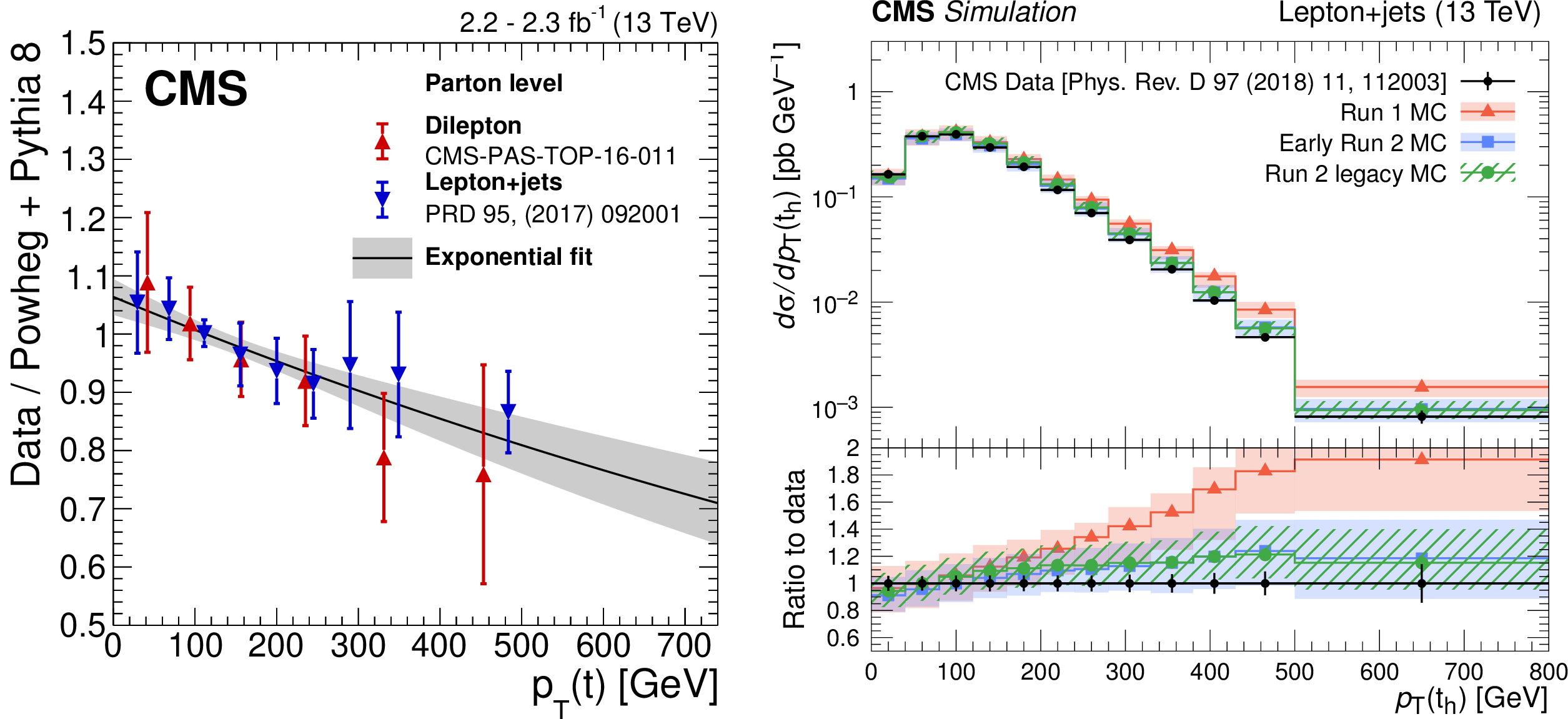
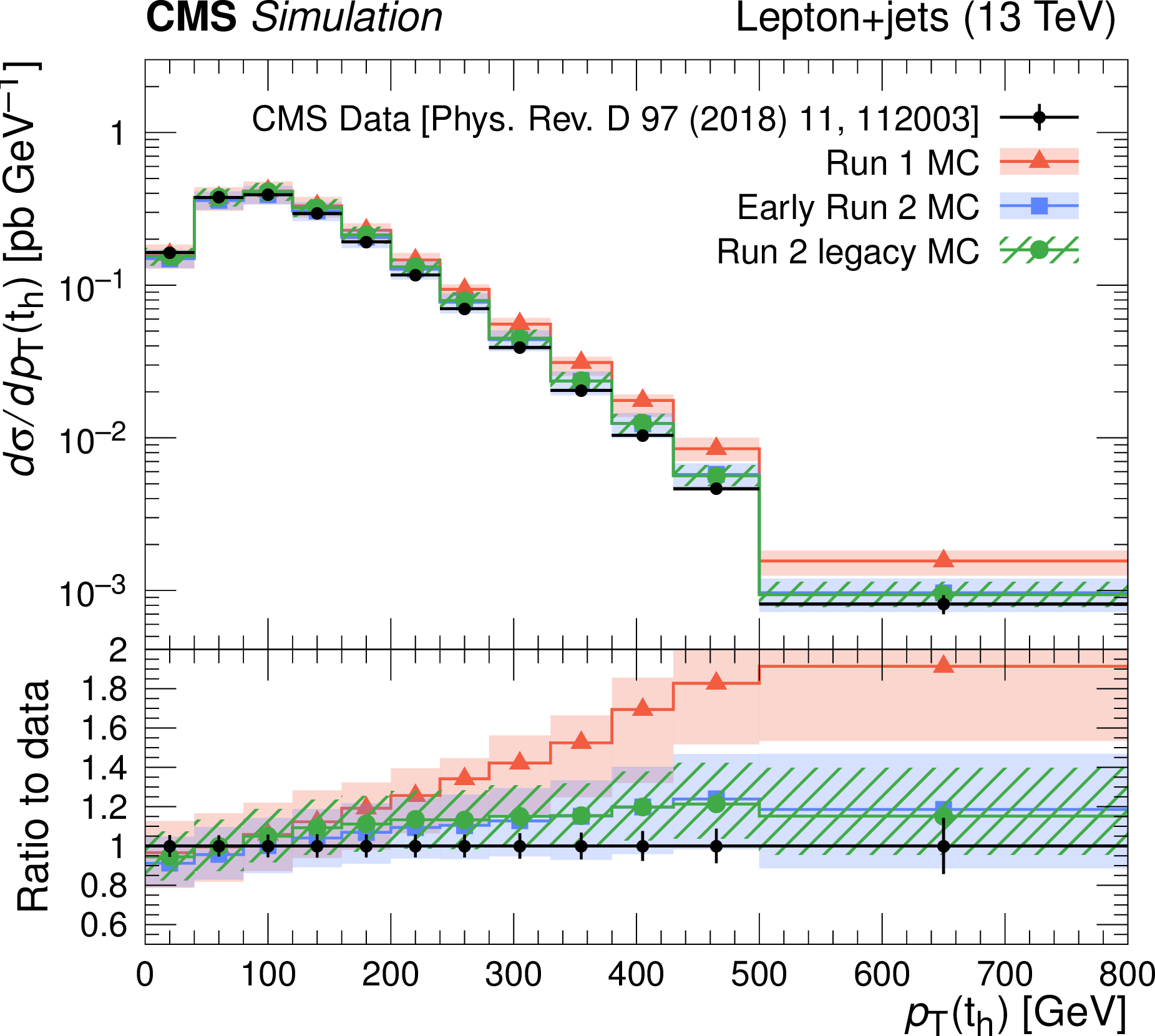
Figure 11:
Left: Ratio of data to POWHEG+PYTHIA-8 (early Run-2) predictions for top quark $ p_{\mathrm{T}} $ in the dilepton (red symbols) and lepton+jets (blue symbols) channels along with an exponential fit (solid line). Right: Distribution of the transverse momentum of hadronically decaying top quark as measured by CMS [139] (black symbols) compared to MC simulations for the generator setups used in Run-1, early Run-2, and Run-2 legacy analyses, presented by bands of different styles. The uncertainty bands include ME scale, ME-PS matching, ISR, and FSR uncertainties. |

png pdf |
Figure 11-a:
Left: Ratio of data to POWHEG+PYTHIA-8 (early Run-2) predictions for top quark $ p_{\mathrm{T}} $ in the dilepton (red symbols) and lepton+jets (blue symbols) channels along with an exponential fit (solid line). Right: Distribution of the transverse momentum of hadronically decaying top quark as measured by CMS [139] (black symbols) compared to MC simulations for the generator setups used in Run-1, early Run-2, and Run-2 legacy analyses, presented by bands of different styles. The uncertainty bands include ME scale, ME-PS matching, ISR, and FSR uncertainties. |
png pdf |
Figure 11-b:
Left: Ratio of data to POWHEG+PYTHIA-8 (early Run-2) predictions for top quark $ p_{\mathrm{T}} $ in the dilepton (red symbols) and lepton+jets (blue symbols) channels along with an exponential fit (solid line). Right: Distribution of the transverse momentum of hadronically decaying top quark as measured by CMS [139] (black symbols) compared to MC simulations for the generator setups used in Run-1, early Run-2, and Run-2 legacy analyses, presented by bands of different styles. The uncertainty bands include ME scale, ME-PS matching, ISR, and FSR uncertainties. |

png pdf |
Figure 12:
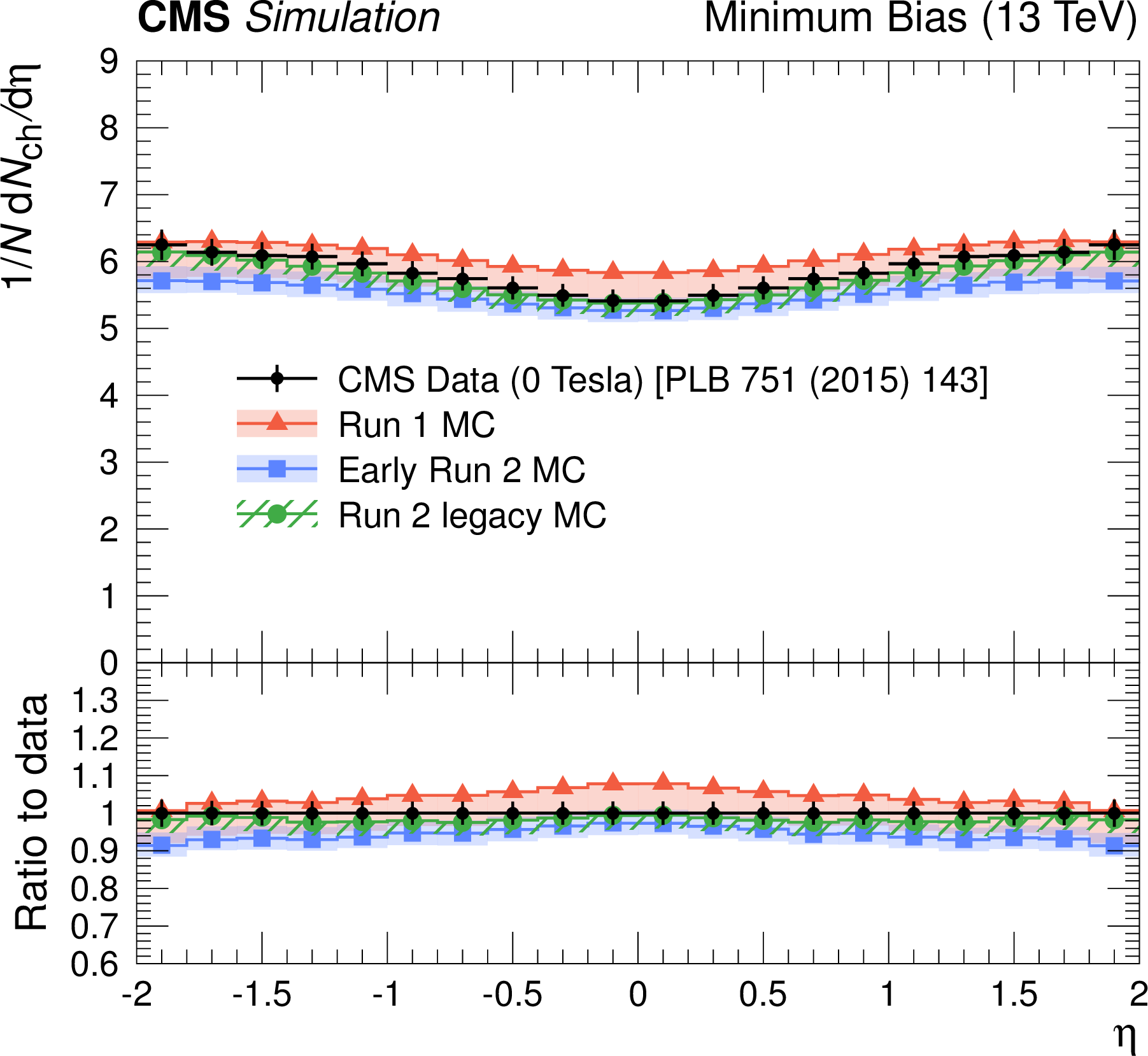
Left: The pseudorapidity density of charged hadrons, $ \mathrm{d} N_{\text{ch}}/\mathrm{d}\eta $, using data from about 170\,000 MB events from inelastic pp collisions using both hit pairs and reconstructed tracks by the CMS experiment [142] at $ \sqrt{s} = $ 13 TeV. Right: The charged-particle $ p_{\mathrm{T}}^{\text{sum}} $ density in the azimuthal region transverse to the direction of the leading charged particle as a function of the $ p_{\mathrm{T}} $ of the leading charged particle, $ p_{\mathrm{T}}^{\text{max}} $, measured by the CMS experiment [143] at $ \sqrt{s} = $ 13 TeV. The predictions of the CMS UE tunes from Run-1 to Run-2 legacy evaluated at 13 TeV are compared with data. The coloured bands represent the variations of the tunes, and error bars on the data points represent the total experimental uncertainty in the data including the model uncertainty. Both distributions are normalised to the total number of events. |
png pdf |
Figure 12-a:
Left: The pseudorapidity density of charged hadrons, $ \mathrm{d} N_{\text{ch}}/\mathrm{d}\eta $, using data from about 170\,000 MB events from inelastic pp collisions using both hit pairs and reconstructed tracks by the CMS experiment [142] at $ \sqrt{s} = $ 13 TeV. Right: The charged-particle $ p_{\mathrm{T}}^{\text{sum}} $ density in the azimuthal region transverse to the direction of the leading charged particle as a function of the $ p_{\mathrm{T}} $ of the leading charged particle, $ p_{\mathrm{T}}^{\text{max}} $, measured by the CMS experiment [143] at $ \sqrt{s} = $ 13 TeV. The predictions of the CMS UE tunes from Run-1 to Run-2 legacy evaluated at 13 TeV are compared with data. The coloured bands represent the variations of the tunes, and error bars on the data points represent the total experimental uncertainty in the data including the model uncertainty. Both distributions are normalised to the total number of events. |

png pdf |
Figure 12-b:
Left: The pseudorapidity density of charged hadrons, $ \mathrm{d} N_{\text{ch}}/\mathrm{d}\eta $, using data from about 170\,000 MB events from inelastic pp collisions using both hit pairs and reconstructed tracks by the CMS experiment [142] at $ \sqrt{s} = $ 13 TeV. Right: The charged-particle $ p_{\mathrm{T}}^{\text{sum}} $ density in the azimuthal region transverse to the direction of the leading charged particle as a function of the $ p_{\mathrm{T}} $ of the leading charged particle, $ p_{\mathrm{T}}^{\text{max}} $, measured by the CMS experiment [143] at $ \sqrt{s} = $ 13 TeV. The predictions of the CMS UE tunes from Run-1 to Run-2 legacy evaluated at 13 TeV are compared with data. The coloured bands represent the variations of the tunes, and error bars on the data points represent the total experimental uncertainty in the data including the model uncertainty. Both distributions are normalised to the total number of events. |

png pdf |
Figure 13:
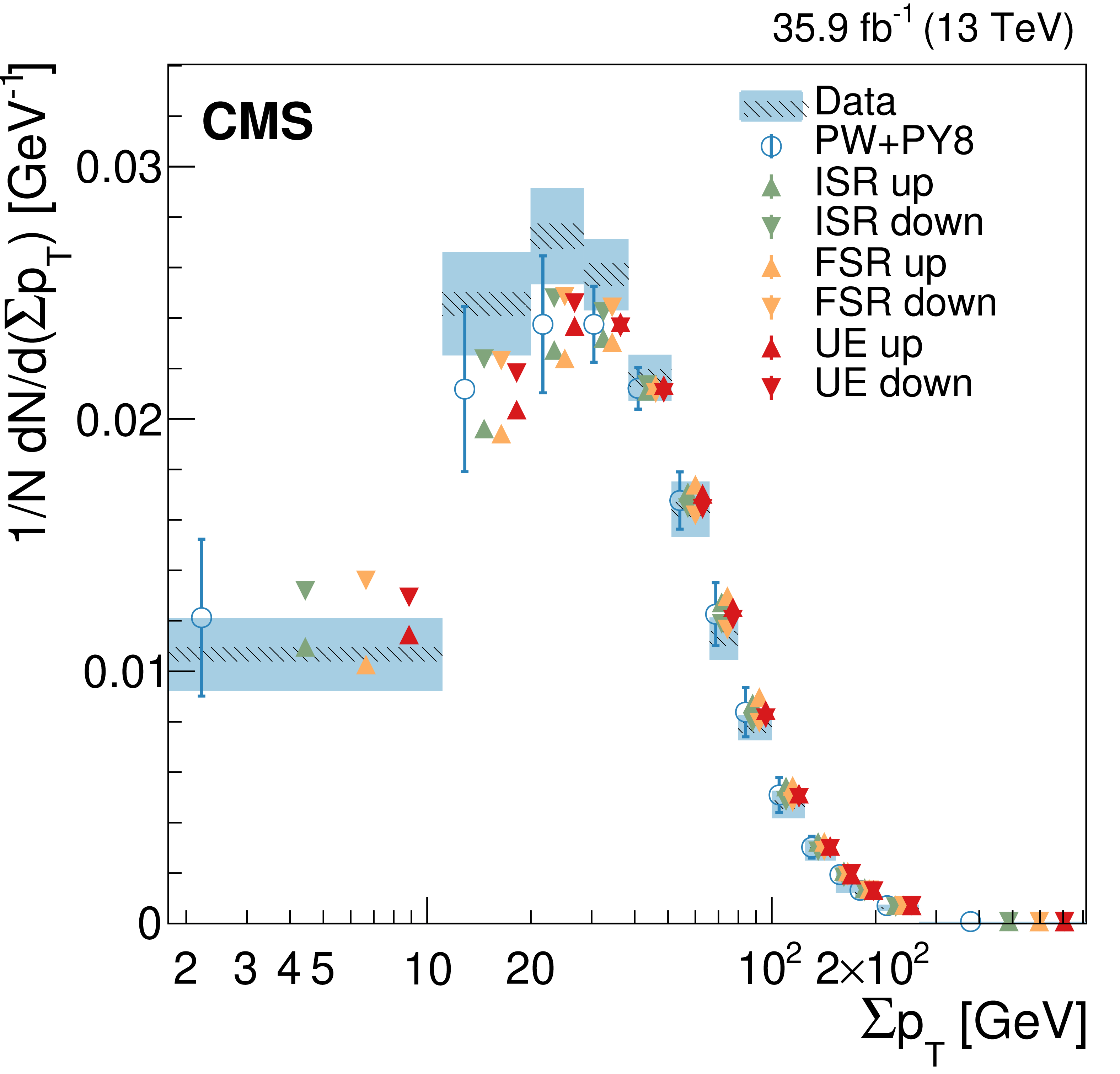
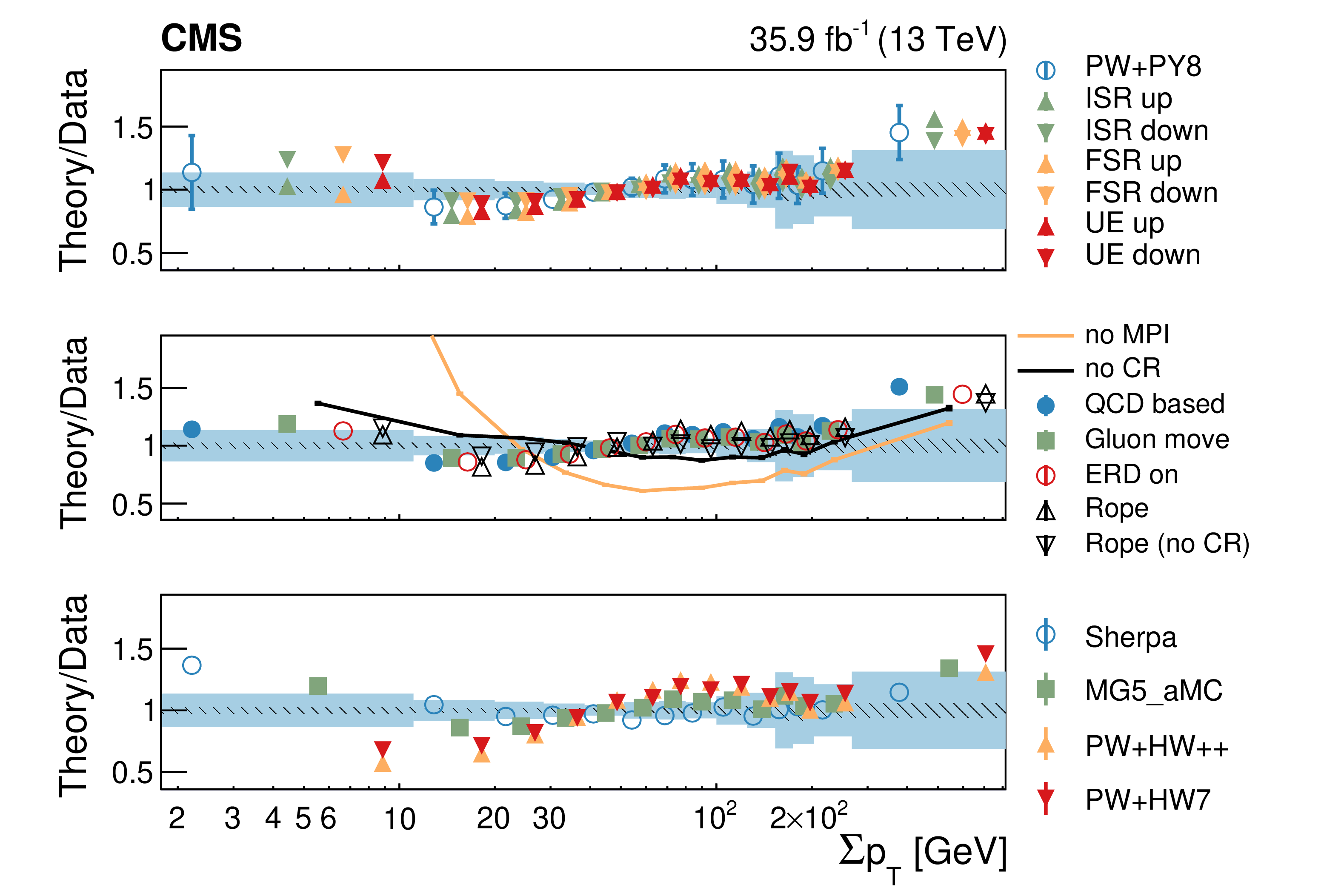
Left: Normalised differential cross section as a function of $ \sum p_{\mathrm{T}} $ of charged particles in the UE in $ \mathrm{t} \overline{\mathrm{t}} $ events, compared to the predictions of different models. The data (coloured boxes) are compared to the nominal POWHEG+PYTHIA-8 predictions and to the expectations obtained from varied $ \alpha_\mathrm{S}^{\text{ISR}}(m_{\mathrm{Z}}) $ or $ \alpha_\mathrm{S}^{\text{FSR}}(m_{\mathrm{Z}}) $ POWHEG+PYTHIA-8 setups (markers). In the case of the POWHEG+PYTHIA-8 setup, the error bar represents the envelope obtained by varying the main parameters of the CEUP8M2T4 tune, according to their uncertainties. This envelope includes the variation of the CR model, $ \alpha_\mathrm{S}^{\text{ISR}}(m_{\mathrm{Z}}) $, $ \alpha_\mathrm{S}^{\text{FSR}}(m_{\mathrm{Z}}) $, the $ h_{\text{damp}} $ parameter, and the $ \mu_{\mathrm{r}} $/$ \mu_{\mathrm{f}} $ scales at the ME level. Right: The different panels show the ratio between each model tested and the data. The shaded (hatched) band represents the total (statistical) uncertainty of the data, while the error bars represent either the total uncertainty of the POWHEG+PYTHIA-8 setup, or the statistical uncertainty of the other MC simulation setups. Figures taken from Ref. [144]. |
png pdf |
Figure 13-a:
Left: Normalised differential cross section as a function of $ \sum p_{\mathrm{T}} $ of charged particles in the UE in $ \mathrm{t} \overline{\mathrm{t}} $ events, compared to the predictions of different models. The data (coloured boxes) are compared to the nominal POWHEG+PYTHIA-8 predictions and to the expectations obtained from varied $ \alpha_\mathrm{S}^{\text{ISR}}(m_{\mathrm{Z}}) $ or $ \alpha_\mathrm{S}^{\text{FSR}}(m_{\mathrm{Z}}) $ POWHEG+PYTHIA-8 setups (markers). In the case of the POWHEG+PYTHIA-8 setup, the error bar represents the envelope obtained by varying the main parameters of the CEUP8M2T4 tune, according to their uncertainties. This envelope includes the variation of the CR model, $ \alpha_\mathrm{S}^{\text{ISR}}(m_{\mathrm{Z}}) $, $ \alpha_\mathrm{S}^{\text{FSR}}(m_{\mathrm{Z}}) $, the $ h_{\text{damp}} $ parameter, and the $ \mu_{\mathrm{r}} $/$ \mu_{\mathrm{f}} $ scales at the ME level. Right: The different panels show the ratio between each model tested and the data. The shaded (hatched) band represents the total (statistical) uncertainty of the data, while the error bars represent either the total uncertainty of the POWHEG+PYTHIA-8 setup, or the statistical uncertainty of the other MC simulation setups. Figures taken from Ref. [144]. |
png pdf |
Figure 13-b:
Left: Normalised differential cross section as a function of $ \sum p_{\mathrm{T}} $ of charged particles in the UE in $ \mathrm{t} \overline{\mathrm{t}} $ events, compared to the predictions of different models. The data (coloured boxes) are compared to the nominal POWHEG+PYTHIA-8 predictions and to the expectations obtained from varied $ \alpha_\mathrm{S}^{\text{ISR}}(m_{\mathrm{Z}}) $ or $ \alpha_\mathrm{S}^{\text{FSR}}(m_{\mathrm{Z}}) $ POWHEG+PYTHIA-8 setups (markers). In the case of the POWHEG+PYTHIA-8 setup, the error bar represents the envelope obtained by varying the main parameters of the CEUP8M2T4 tune, according to their uncertainties. This envelope includes the variation of the CR model, $ \alpha_\mathrm{S}^{\text{ISR}}(m_{\mathrm{Z}}) $, $ \alpha_\mathrm{S}^{\text{FSR}}(m_{\mathrm{Z}}) $, the $ h_{\text{damp}} $ parameter, and the $ \mu_{\mathrm{r}} $/$ \mu_{\mathrm{f}} $ scales at the ME level. Right: The different panels show the ratio between each model tested and the data. The shaded (hatched) band represents the total (statistical) uncertainty of the data, while the error bars represent either the total uncertainty of the POWHEG+PYTHIA-8 setup, or the statistical uncertainty of the other MC simulation setups. Figures taken from Ref. [144]. |
png pdf |
Figure 14:
Measured distribution of the pull angle in $ \mathrm{t} \overline{\mathrm{t}} $ events taken at 8 TeV recorded by ATLAS [154] (points with vertical error bars) compared to MC simulations for the generator setups used in Run-1, early Run-2, and Run-2 legacy analyses, presented by bands of different styles. The uncertainty bands illustrate the uncertainties resulting from colour reconnection effects, as estimated by variations described in the main text. The same variations are applied in CMS top quark mass measurements. |
png pdf |
Figure 15:
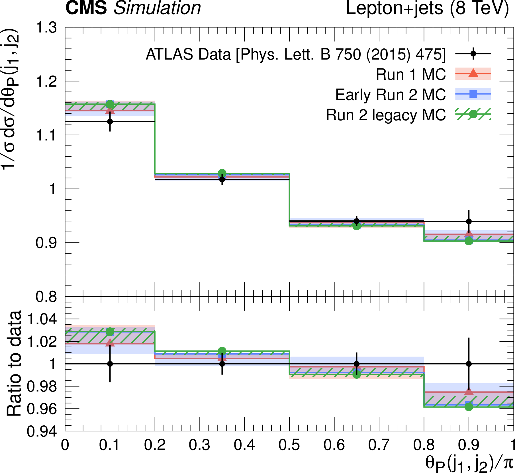
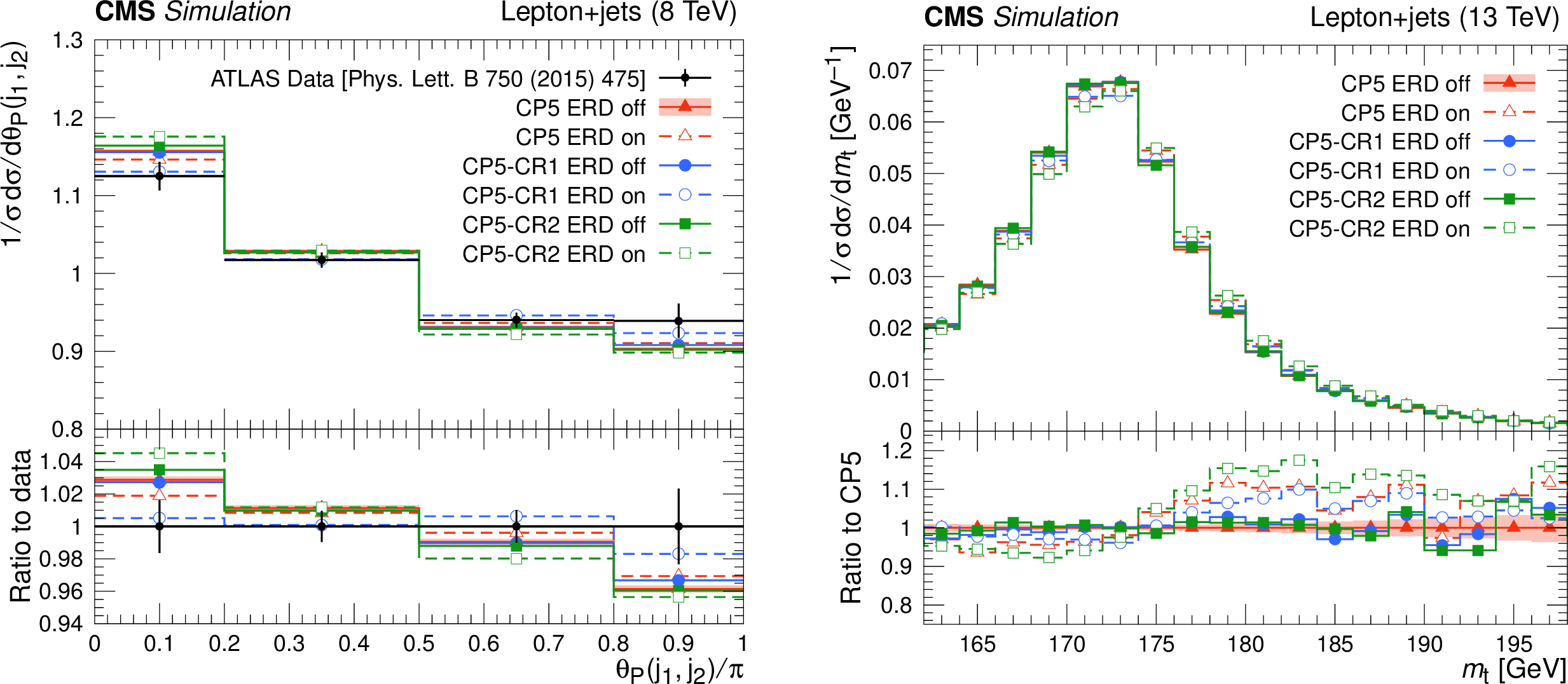
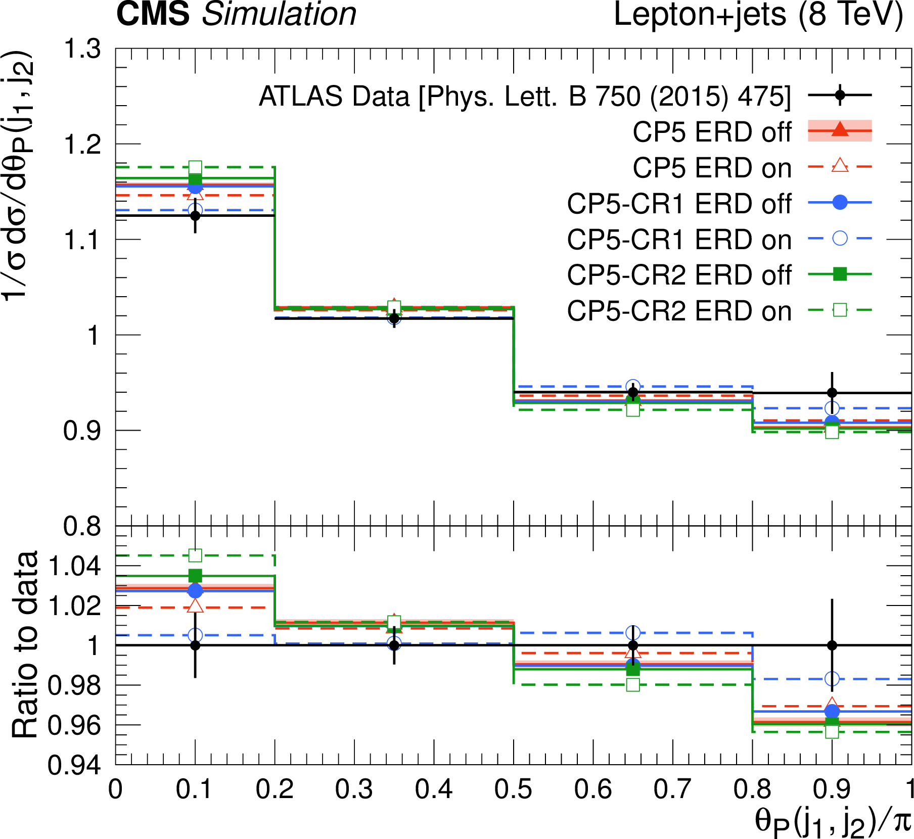
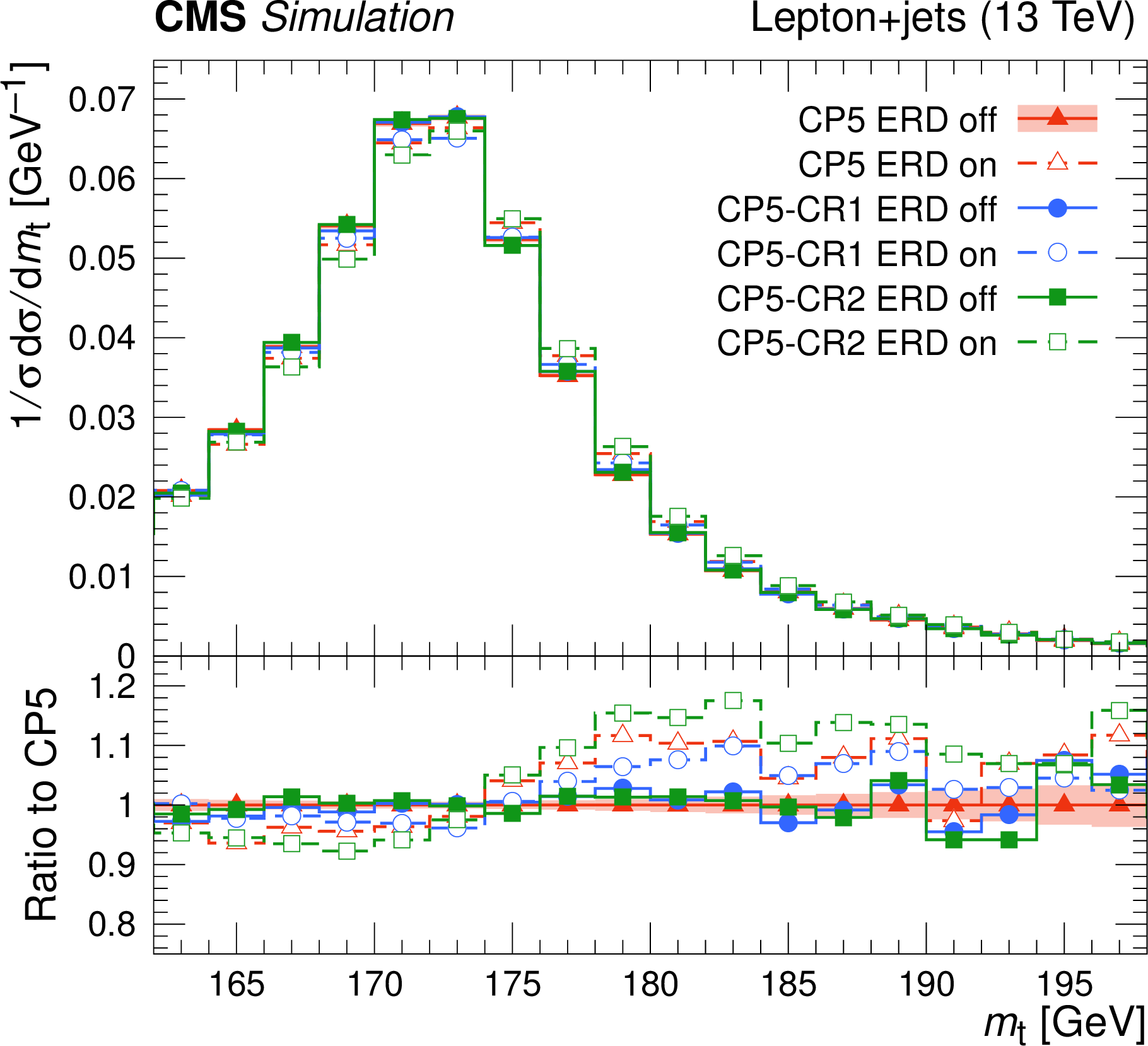
Normalised $ \mathrm{t} \overline{\mathrm{t}} $ differential cross section for the pull angle between jets from the W boson in hadronic top quark decays, calculated from the charged constituents of the jets, measured by the ATLAS experiment using $ \sqrt{s} = $ 8 TeV data [154] to investigate colour flow (left). The predictions from POWHEG+PYTHIA-8 using different tune configurations are compared with data. The statistical uncertainties in the predictions are represented by the coloured band and the vertical bars. The coloured band and error bars on the data points represent the total experimental uncertainty in the data. The invariant mass reconstructed from the hadronically decaying top quark candidates at the generator level (right). The coloured band and the vertical bars represent the statistical uncertainty in the predictions. Figures adapted from Ref. [152]. |
png pdf |
Figure 15-a:
Normalised $ \mathrm{t} \overline{\mathrm{t}} $ differential cross section for the pull angle between jets from the W boson in hadronic top quark decays, calculated from the charged constituents of the jets, measured by the ATLAS experiment using $ \sqrt{s} = $ 8 TeV data [154] to investigate colour flow (left). The predictions from POWHEG+PYTHIA-8 using different tune configurations are compared with data. The statistical uncertainties in the predictions are represented by the coloured band and the vertical bars. The coloured band and error bars on the data points represent the total experimental uncertainty in the data. The invariant mass reconstructed from the hadronically decaying top quark candidates at the generator level (right). The coloured band and the vertical bars represent the statistical uncertainty in the predictions. Figures adapted from Ref. [152]. |
png pdf |
Figure 15-b:
Normalised $ \mathrm{t} \overline{\mathrm{t}} $ differential cross section for the pull angle between jets from the W boson in hadronic top quark decays, calculated from the charged constituents of the jets, measured by the ATLAS experiment using $ \sqrt{s} = $ 8 TeV data [154] to investigate colour flow (left). The predictions from POWHEG+PYTHIA-8 using different tune configurations are compared with data. The statistical uncertainties in the predictions are represented by the coloured band and the vertical bars. The coloured band and error bars on the data points represent the total experimental uncertainty in the data. The invariant mass reconstructed from the hadronically decaying top quark candidates at the generator level (right). The coloured band and the vertical bars represent the statistical uncertainty in the predictions. Figures adapted from Ref. [152]. |

png pdf |
Figure 16:
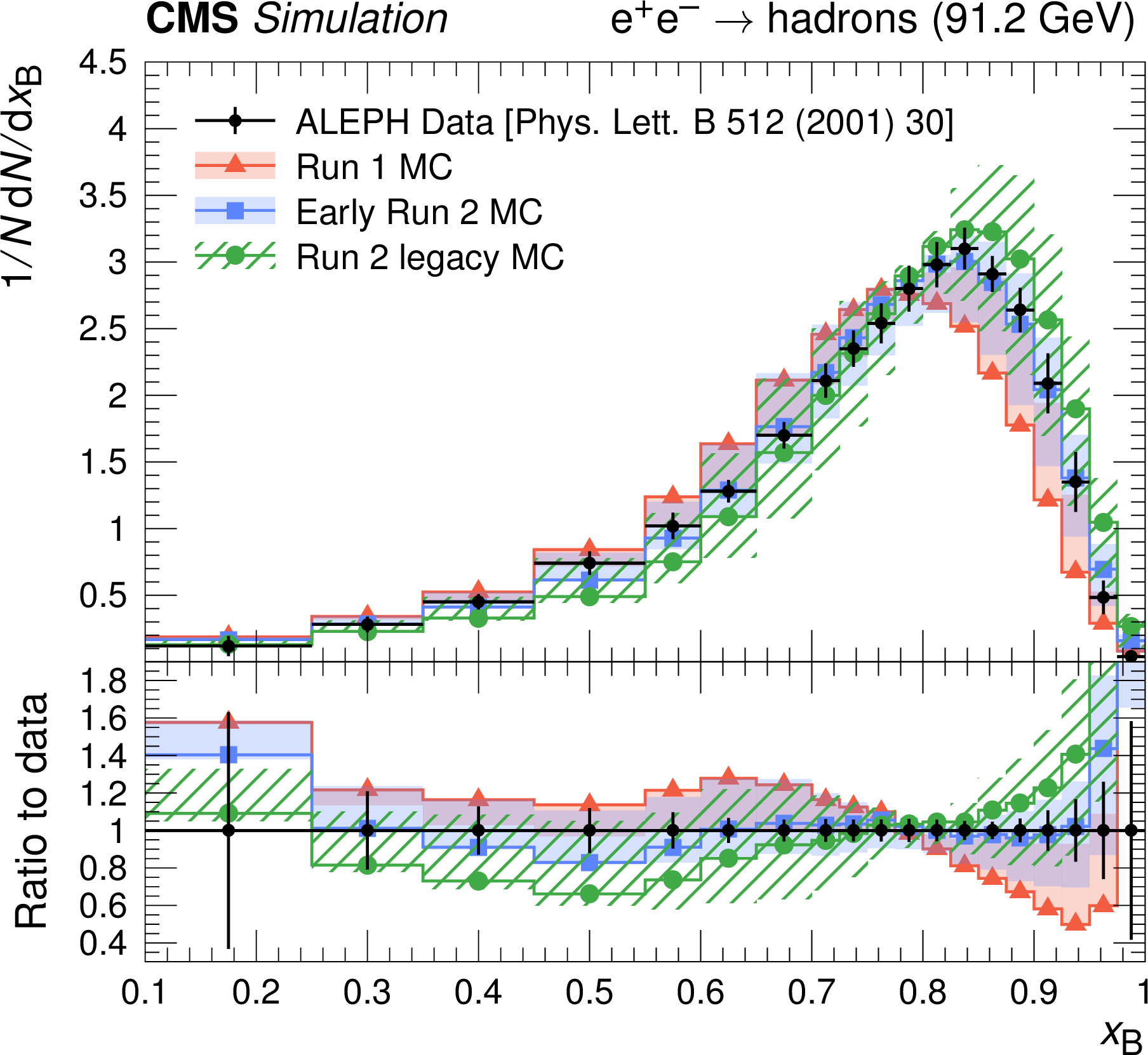
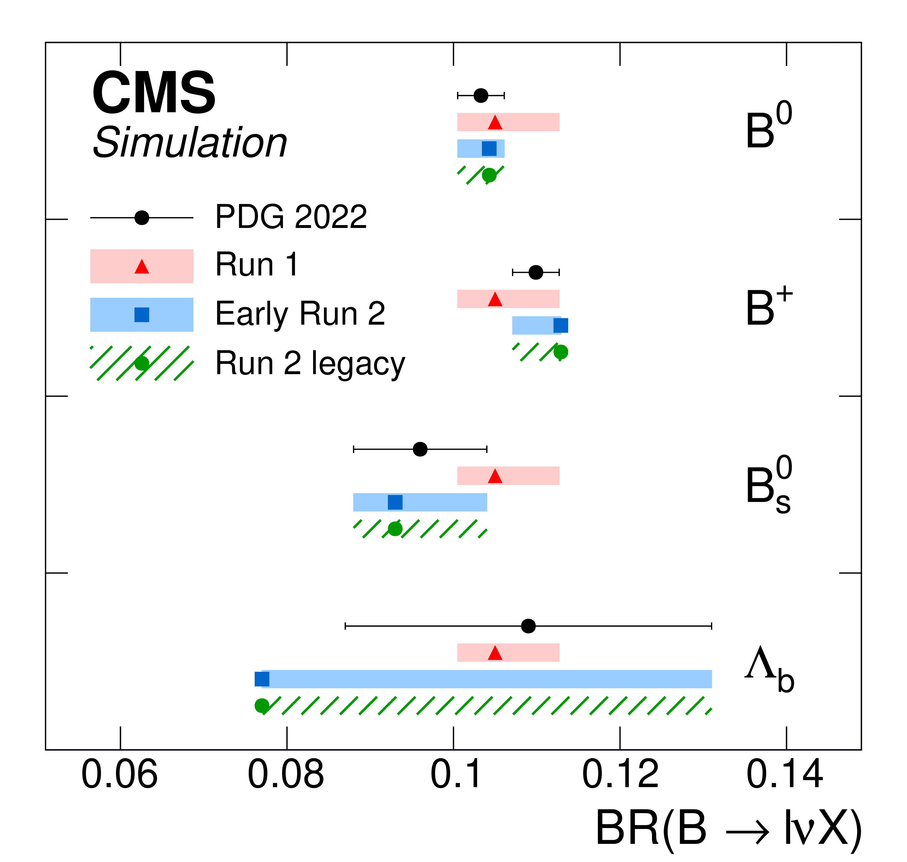
Distribution of the b quark fragmentation function normalised to the number of b hadrons measured by ALEPH in $ \mathrm{e}^+ \mathrm{e}^- $ collisions at $ \sqrt{s}= $ 91.2 GeV [156] (black symbols with vertical error bars showing the total measurement uncertainties) compared to $ \mathrm{e}^+ \mathrm{e}^- $ MC simulations for the generator setups used in Run-1, early Run-2, and Run-2 legacy analyses, presented by bands of different styles (left). The uncertainty bands are constructed around the default prediction and illustrate the b quark fragmentation uncertainties. The measured semileptonic branching ratios of b hadrons [1] (black symbols) compared to the values in the generator setups (coloured symbols) and their uncertainties, illustrated by shaded bands (right). |
png pdf |
Figure 16-a:
Distribution of the b quark fragmentation function normalised to the number of b hadrons measured by ALEPH in $ \mathrm{e}^+ \mathrm{e}^- $ collisions at $ \sqrt{s}= $ 91.2 GeV [156] (black symbols with vertical error bars showing the total measurement uncertainties) compared to $ \mathrm{e}^+ \mathrm{e}^- $ MC simulations for the generator setups used in Run-1, early Run-2, and Run-2 legacy analyses, presented by bands of different styles (left). The uncertainty bands are constructed around the default prediction and illustrate the b quark fragmentation uncertainties. The measured semileptonic branching ratios of b hadrons [1] (black symbols) compared to the values in the generator setups (coloured symbols) and their uncertainties, illustrated by shaded bands (right). |
png pdf |
Figure 16-b:
Distribution of the b quark fragmentation function normalised to the number of b hadrons measured by ALEPH in $ \mathrm{e}^+ \mathrm{e}^- $ collisions at $ \sqrt{s}= $ 91.2 GeV [156] (black symbols with vertical error bars showing the total measurement uncertainties) compared to $ \mathrm{e}^+ \mathrm{e}^- $ MC simulations for the generator setups used in Run-1, early Run-2, and Run-2 legacy analyses, presented by bands of different styles (left). The uncertainty bands are constructed around the default prediction and illustrate the b quark fragmentation uncertainties. The measured semileptonic branching ratios of b hadrons [1] (black symbols) compared to the values in the generator setups (coloured symbols) and their uncertainties, illustrated by shaded bands (right). |
png pdf |
Figure 17:
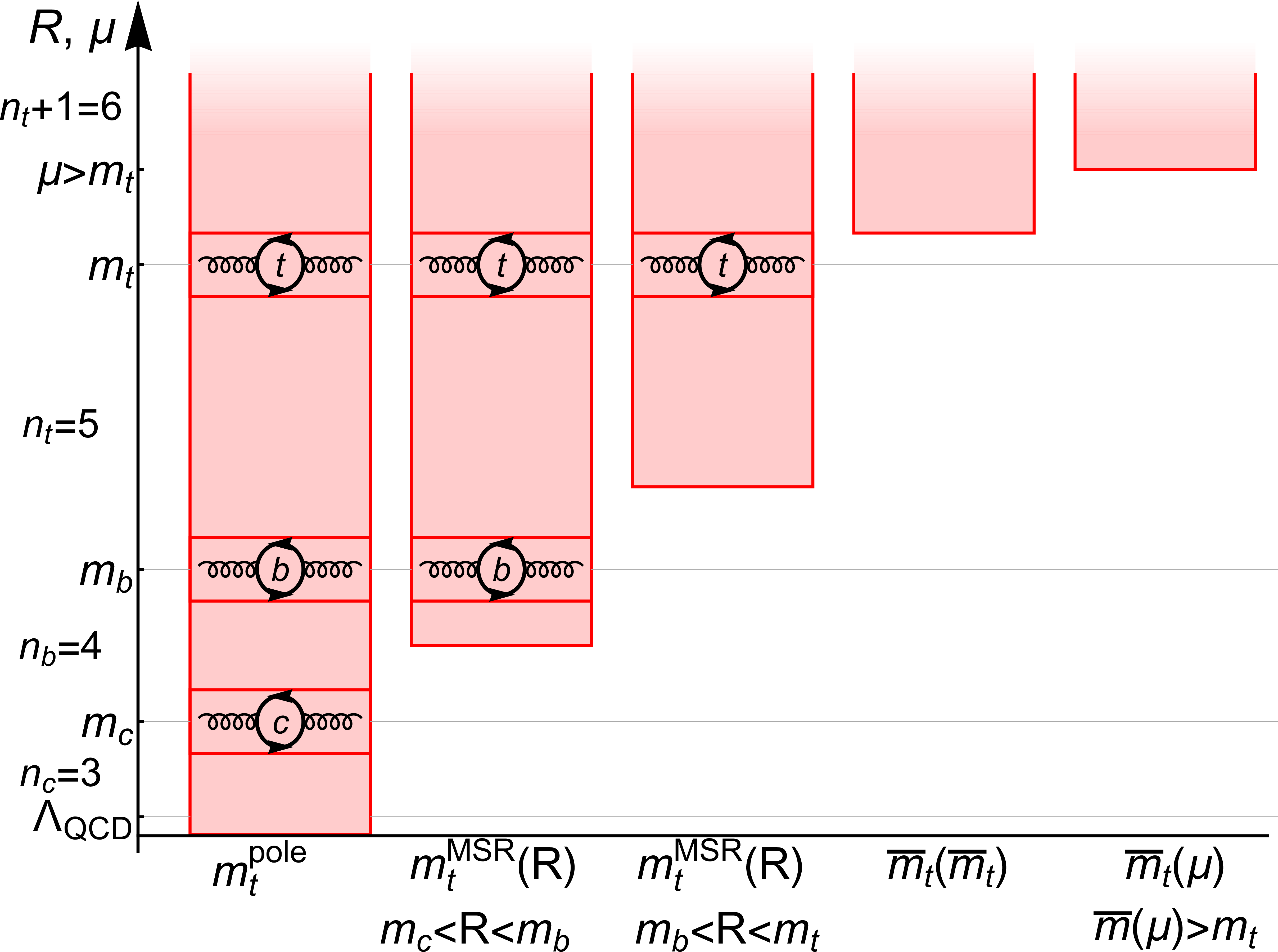
Momenta of the self-energy quantum corrections in the top quark rest frame (red segments), absorbed into the top quark mass parameter in the pole (very left), MSR and $ \mathrm{\overline{MS}} $ schemes for different mass renormalisation scales with respect to the charm and bottom quark masses. The red segments extend to infinite momenta for all top quark mass schemes. The loops inside the red segments illustrate contributions of the virtual top, charm, or bottom quark loops, and $ n_{\mathrm{q}} $ stands for the number of quarks lighter than quark $ \mathrm{q} $, indicating that the MSR and the $ \mathrm{\overline{MS}} $ masses run with different flavour numbers between flavour thresholds, as does the strong coupling constant $ \alpha_\mathrm{S} $. Figure taken from Ref. [188]. |
png pdf |
Figure 18:
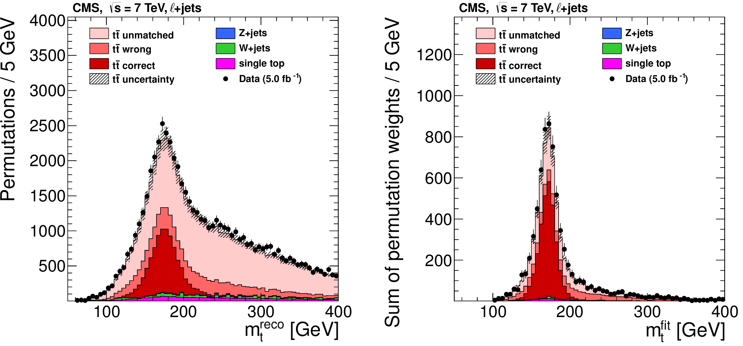
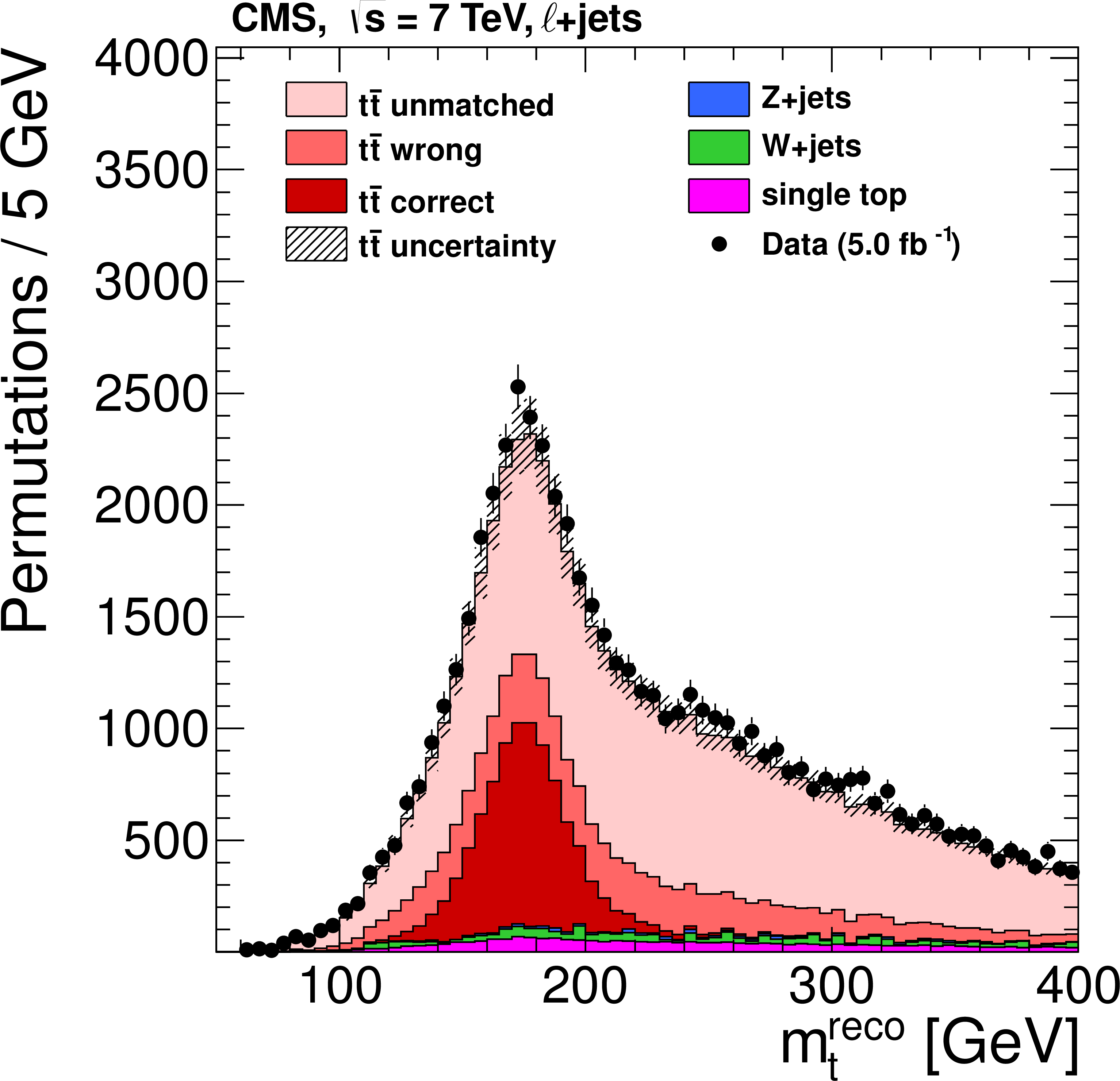
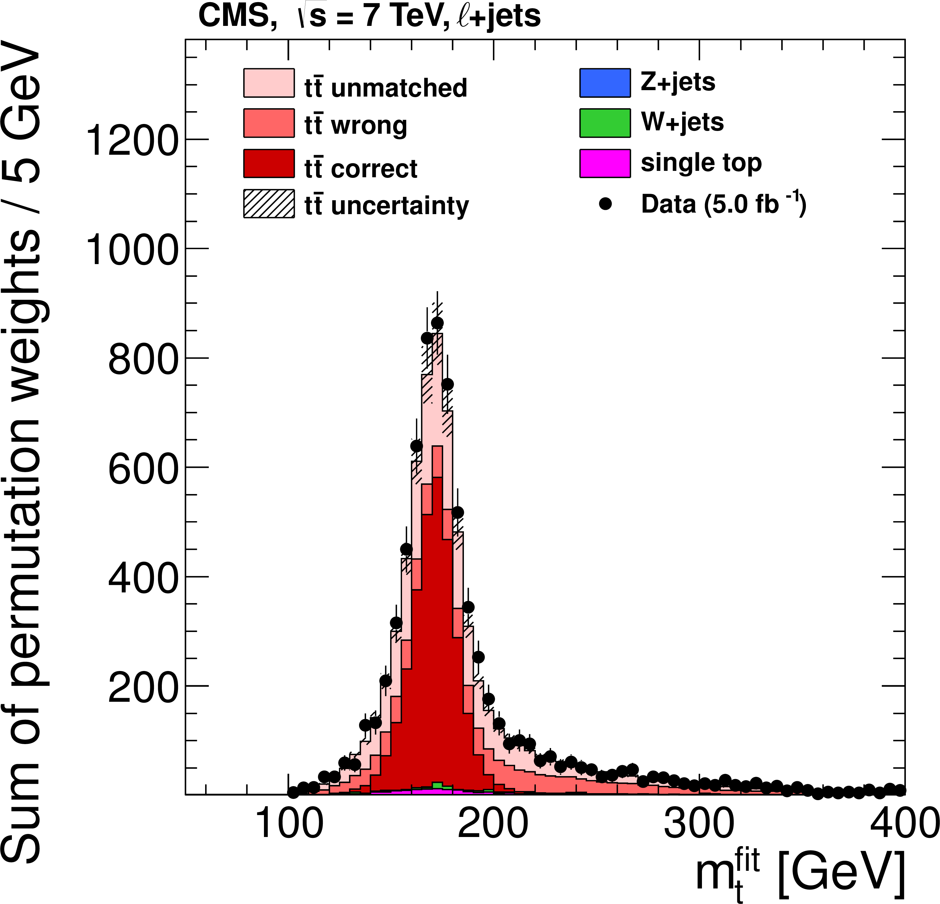
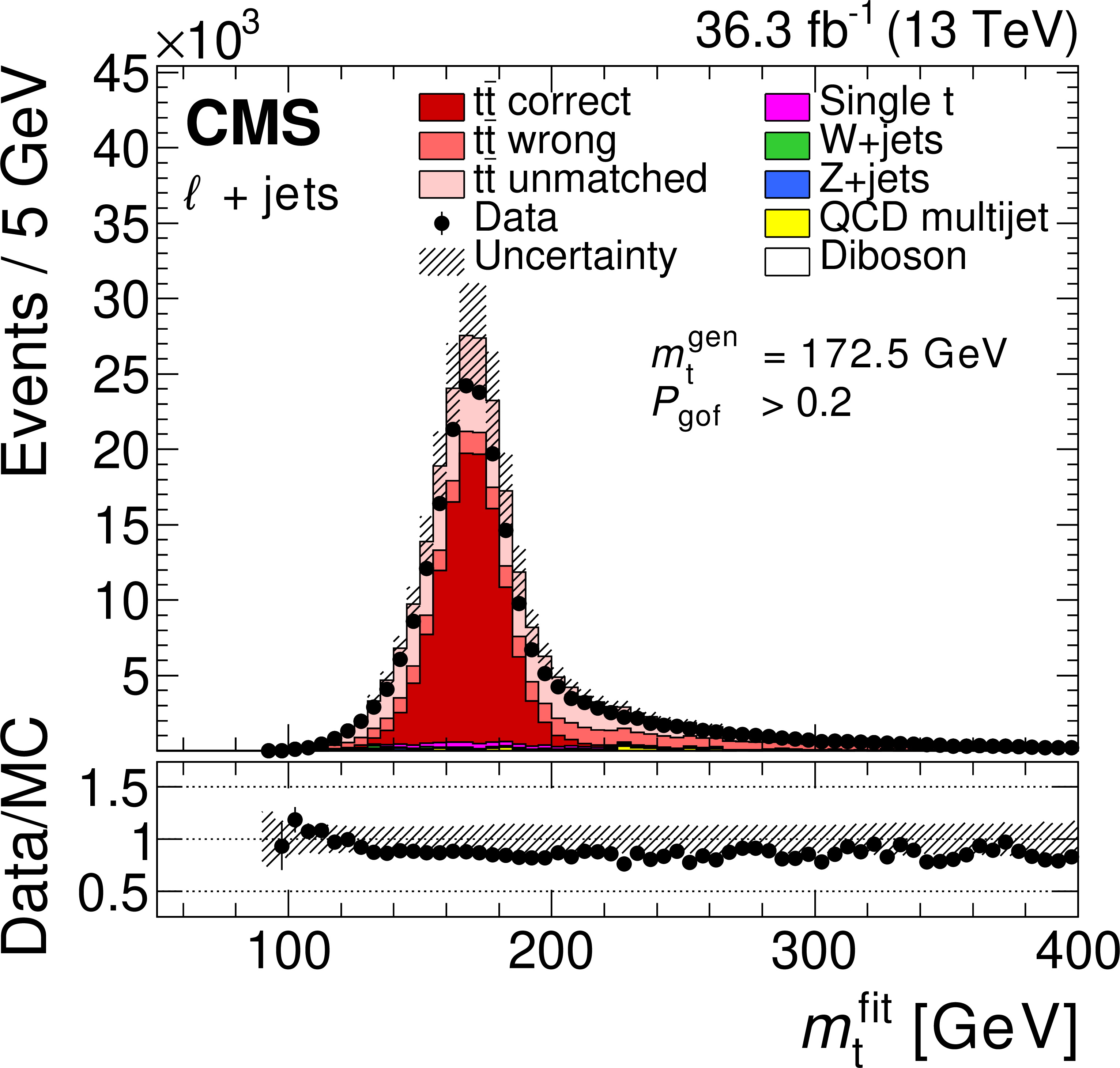
Left: The distribution of the reconstructed top quark mass $ m_{\mathrm{t}}^\text{reco} $ using the jet assignment from the kinematic fit, but the reconstructed jet momenta and no addition selection. Right: The distribution of the top quark mass from the kinematic fit $ m_{\mathrm{t}}^\text{fit} $ with the $ P_{\text{gof}} > $ 0.2 selection. Data are shown as points with vertical error bars showing the statistical uncertainties. The coloured histograms show the simulated signal and background contributions. The simulated signal is decomposed into the contributions from correct, wrong, or unmatched permutations as introduced in Section 2.3. The uncertainty in the predicted $ \mathrm{t} \overline{\mathrm{t}} $ cross section is indicated by the hatched area. In the figures, the default value of $ m_{\mathrm{t}}^\text{gen}= $ 172.5 GeV is used. The reduction of permutations with wrongly assigned jets and the much narrower peak are clearly visible in the $ m_{\mathrm{t}}^\text{fit} $ measurement. Figures taken from Ref. [48]. |
png pdf |
Figure 18-a:
Left: The distribution of the reconstructed top quark mass $ m_{\mathrm{t}}^\text{reco} $ using the jet assignment from the kinematic fit, but the reconstructed jet momenta and no addition selection. Right: The distribution of the top quark mass from the kinematic fit $ m_{\mathrm{t}}^\text{fit} $ with the $ P_{\text{gof}} > $ 0.2 selection. Data are shown as points with vertical error bars showing the statistical uncertainties. The coloured histograms show the simulated signal and background contributions. The simulated signal is decomposed into the contributions from correct, wrong, or unmatched permutations as introduced in Section 2.3. The uncertainty in the predicted $ \mathrm{t} \overline{\mathrm{t}} $ cross section is indicated by the hatched area. In the figures, the default value of $ m_{\mathrm{t}}^\text{gen}= $ 172.5 GeV is used. The reduction of permutations with wrongly assigned jets and the much narrower peak are clearly visible in the $ m_{\mathrm{t}}^\text{fit} $ measurement. Figures taken from Ref. [48]. |
png pdf |
Figure 18-b:
Left: The distribution of the reconstructed top quark mass $ m_{\mathrm{t}}^\text{reco} $ using the jet assignment from the kinematic fit, but the reconstructed jet momenta and no addition selection. Right: The distribution of the top quark mass from the kinematic fit $ m_{\mathrm{t}}^\text{fit} $ with the $ P_{\text{gof}} > $ 0.2 selection. Data are shown as points with vertical error bars showing the statistical uncertainties. The coloured histograms show the simulated signal and background contributions. The simulated signal is decomposed into the contributions from correct, wrong, or unmatched permutations as introduced in Section 2.3. The uncertainty in the predicted $ \mathrm{t} \overline{\mathrm{t}} $ cross section is indicated by the hatched area. In the figures, the default value of $ m_{\mathrm{t}}^\text{gen}= $ 172.5 GeV is used. The reduction of permutations with wrongly assigned jets and the much narrower peak are clearly visible in the $ m_{\mathrm{t}}^\text{fit} $ measurement. Figures taken from Ref. [48]. |
png pdf |
Figure 19:
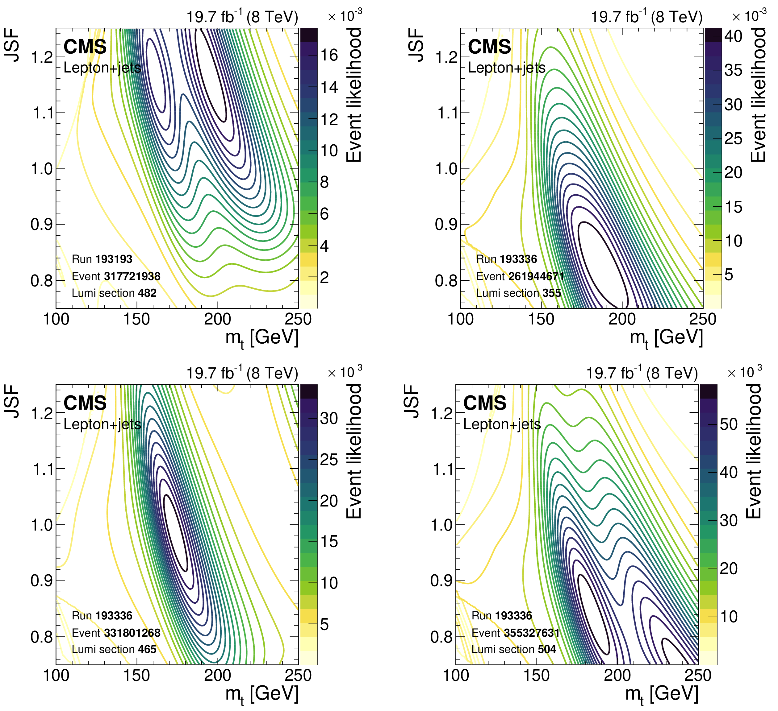
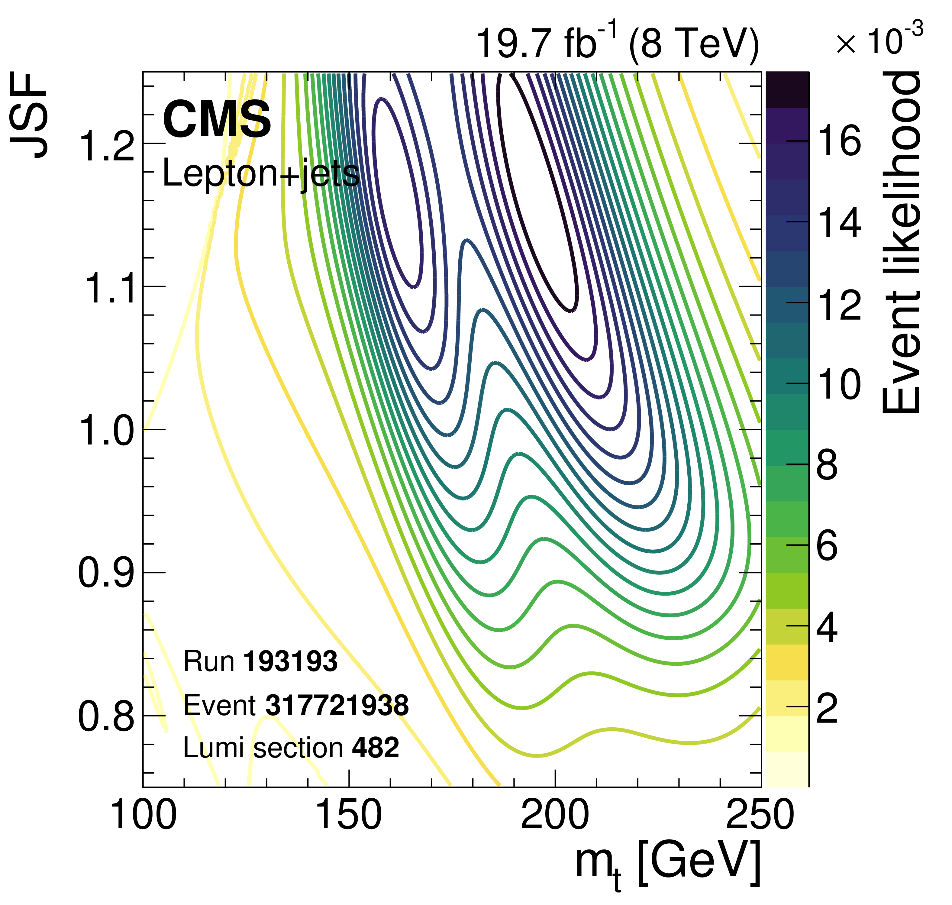
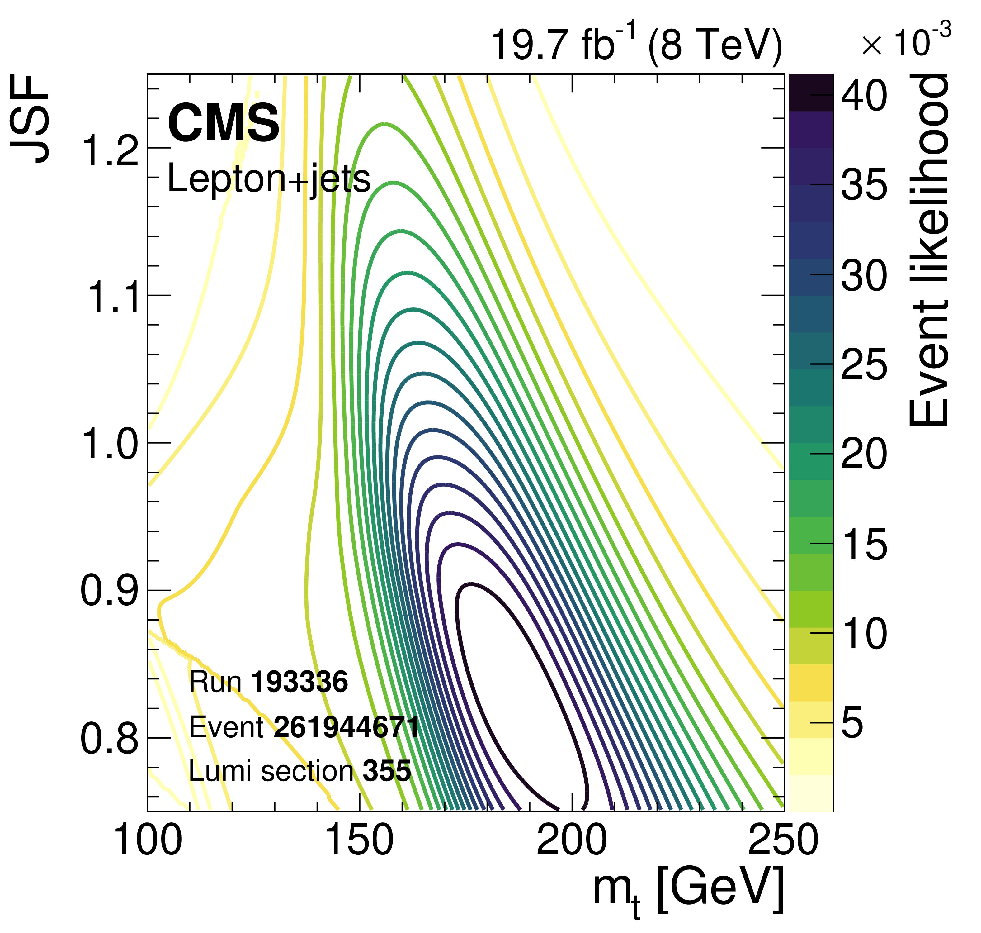
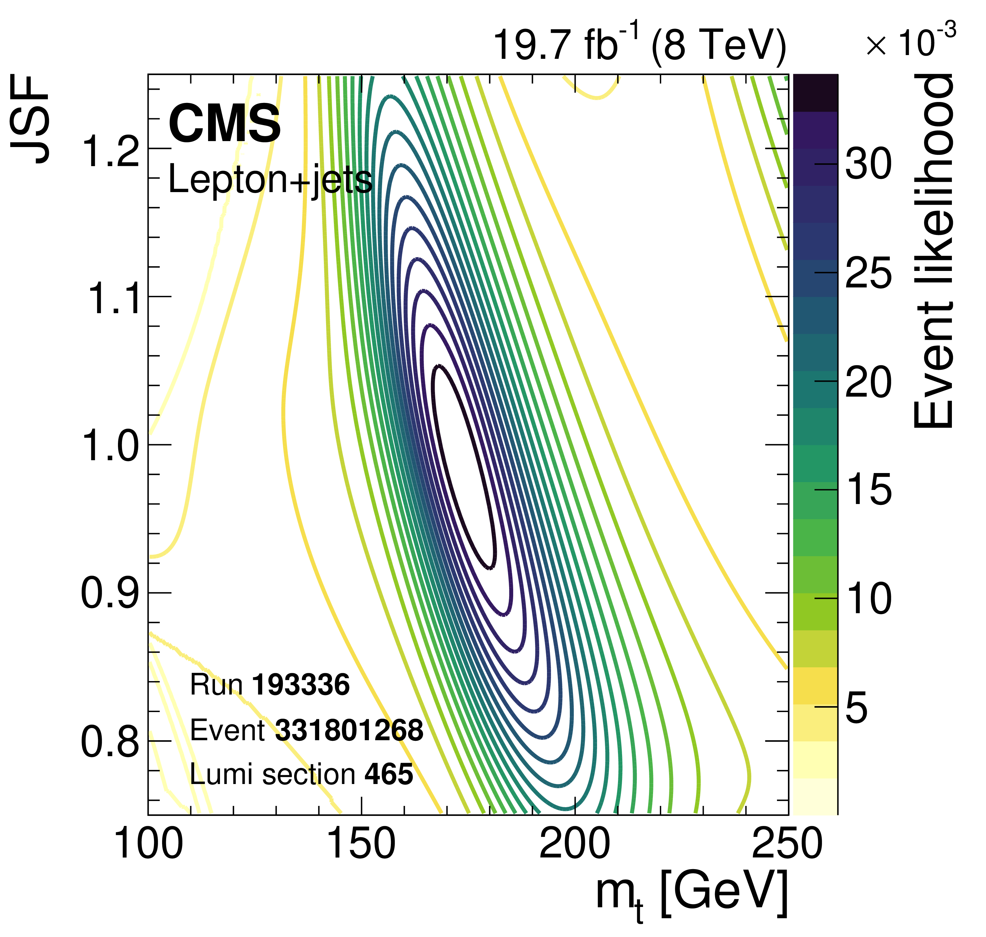
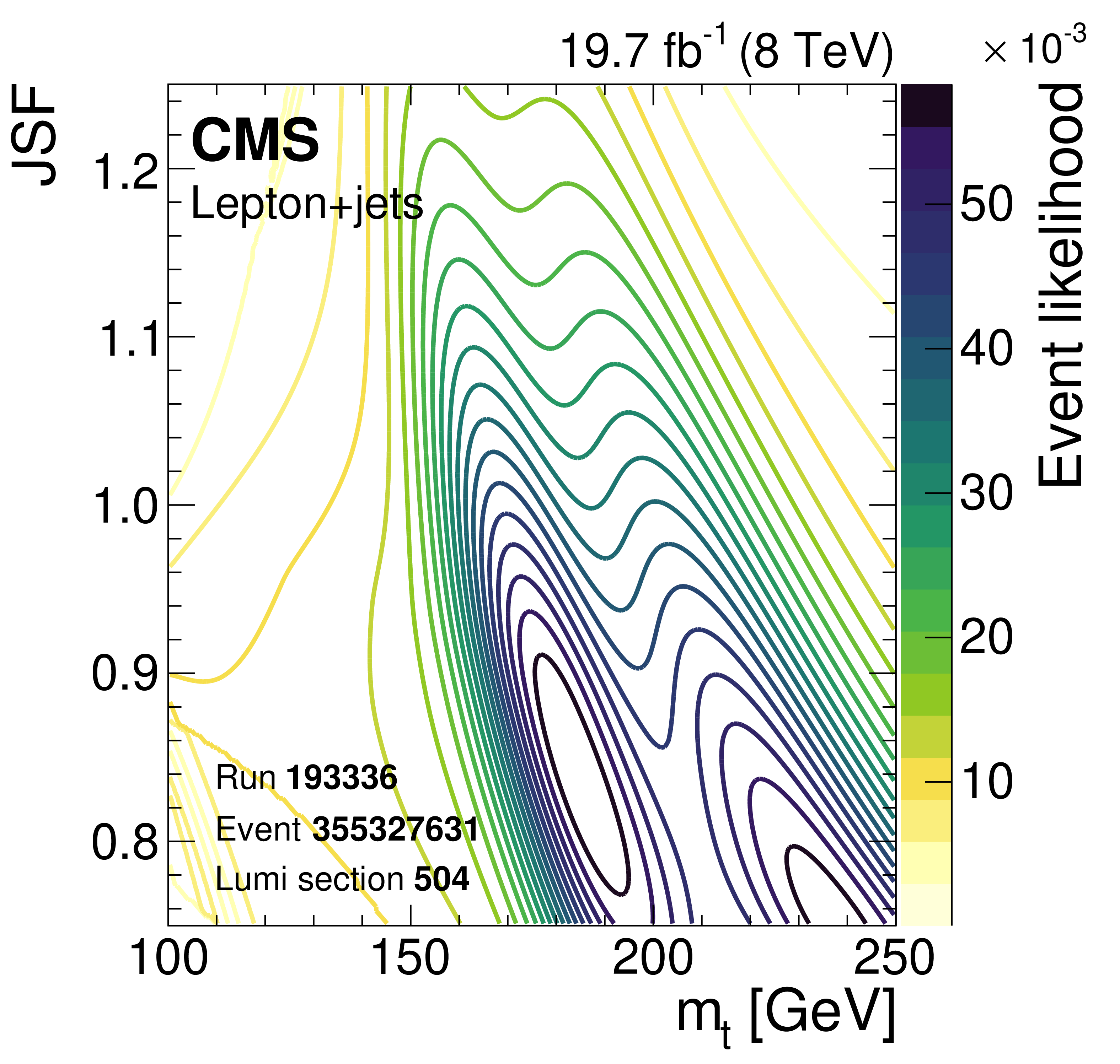
Contours of the likelihood of $ m_{\mathrm{t}} $ and $ \text{JSF} $ values for single events in the Run-1 CMS measurement [53]. |
png pdf |
Figure 19-a:
Contours of the likelihood of $ m_{\mathrm{t}} $ and $ \text{JSF} $ values for single events in the Run-1 CMS measurement [53]. |
png pdf |
Figure 19-b:
Contours of the likelihood of $ m_{\mathrm{t}} $ and $ \text{JSF} $ values for single events in the Run-1 CMS measurement [53]. |
png pdf |
Figure 19-c:
Contours of the likelihood of $ m_{\mathrm{t}} $ and $ \text{JSF} $ values for single events in the Run-1 CMS measurement [53]. |
png pdf |
Figure 19-d:
Contours of the likelihood of $ m_{\mathrm{t}} $ and $ \text{JSF} $ values for single events in the Run-1 CMS measurement [53]. |
png pdf |
Figure 20:
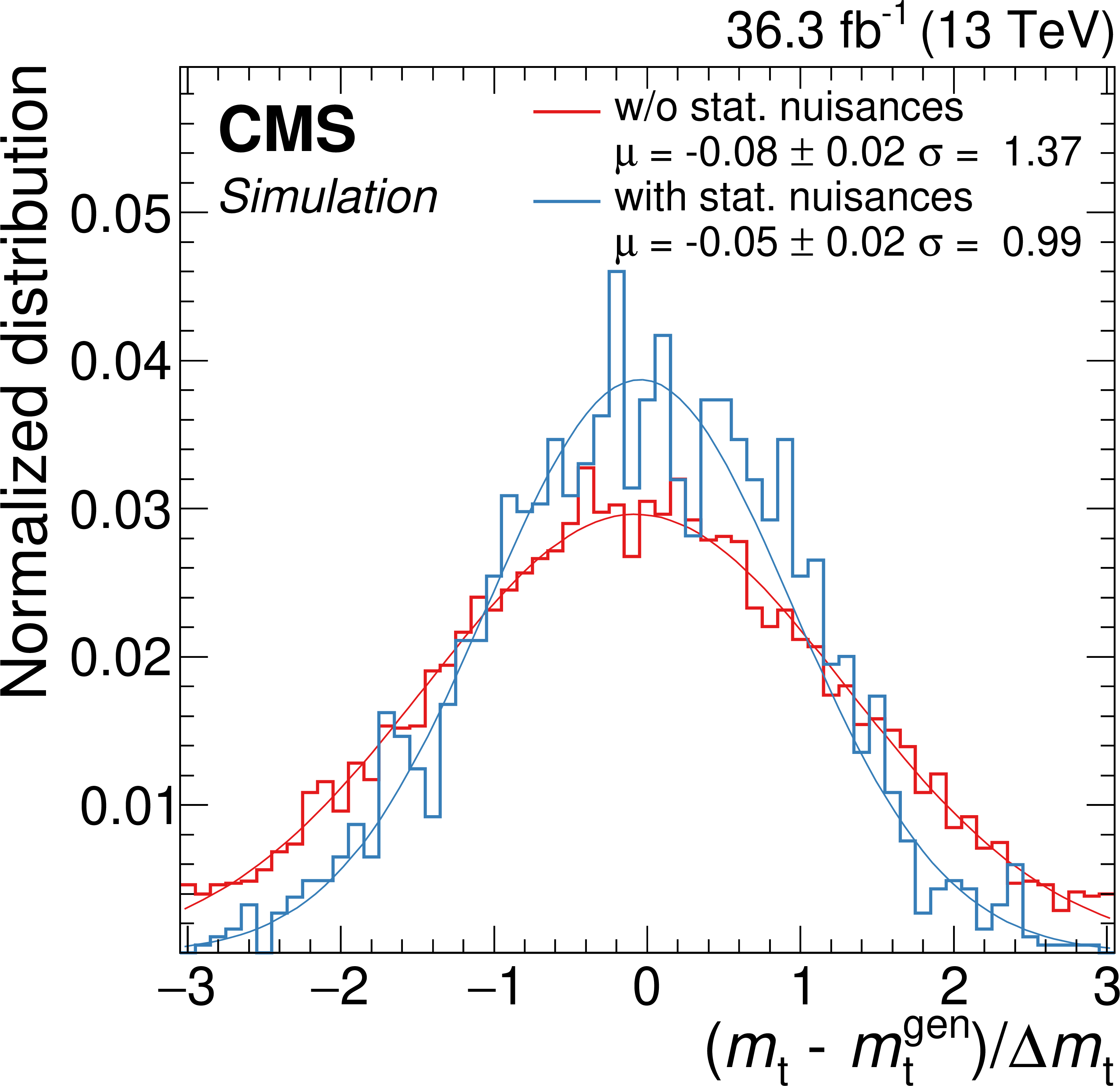
The difference between the measured and generated $ m_{\mathrm{t}} $ values, divided by the uncertainty reported by the fit from pseudo-experiments without (red) or with (blue) the additional nuisance parameters for the finite sample sizes. Also included in the legend are the $ \mu $ and $ \sigma $ parameters of Gaussian functions (red and blue lines) fit to the histograms. Figure taken from Ref. [71]. |
png pdf |
Figure 21:
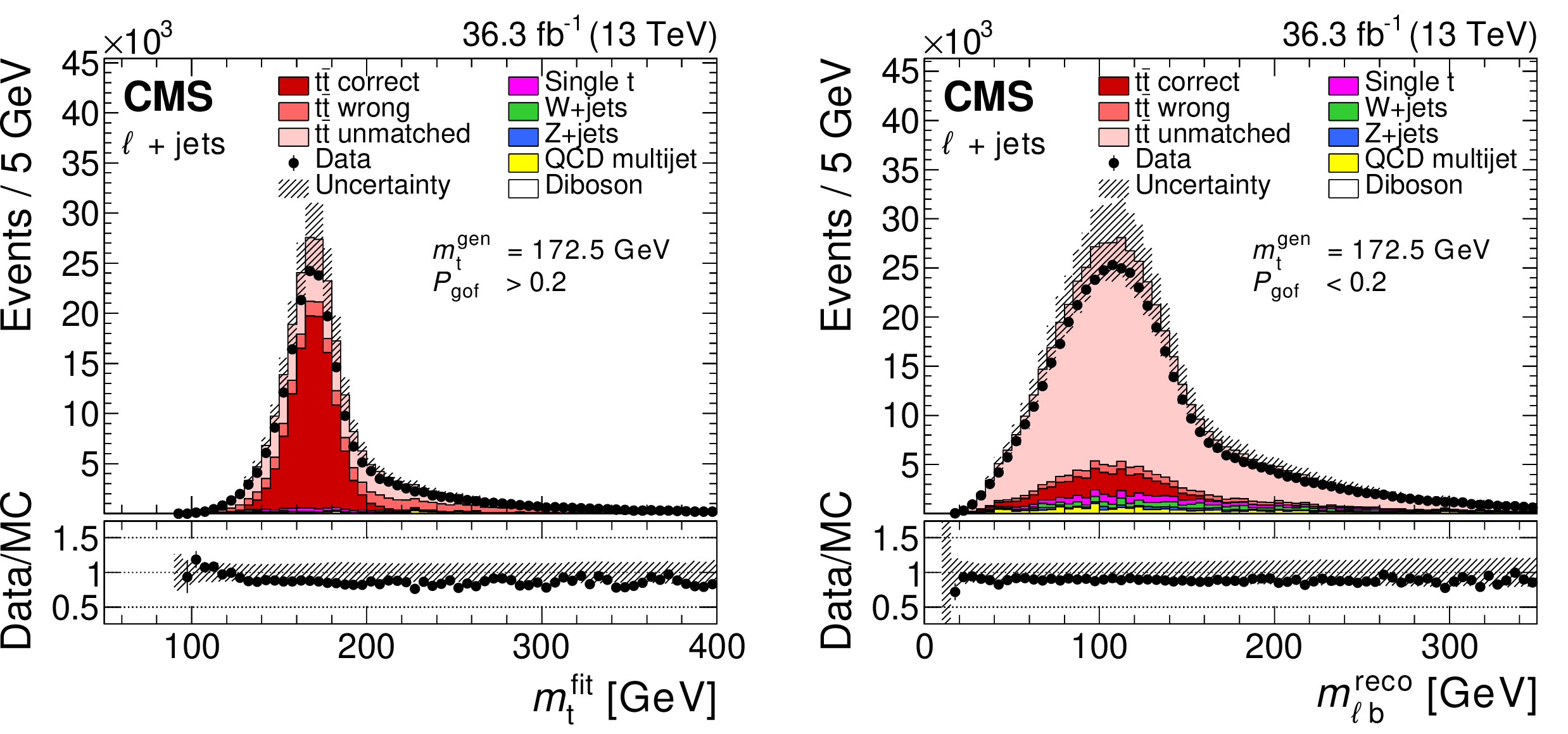
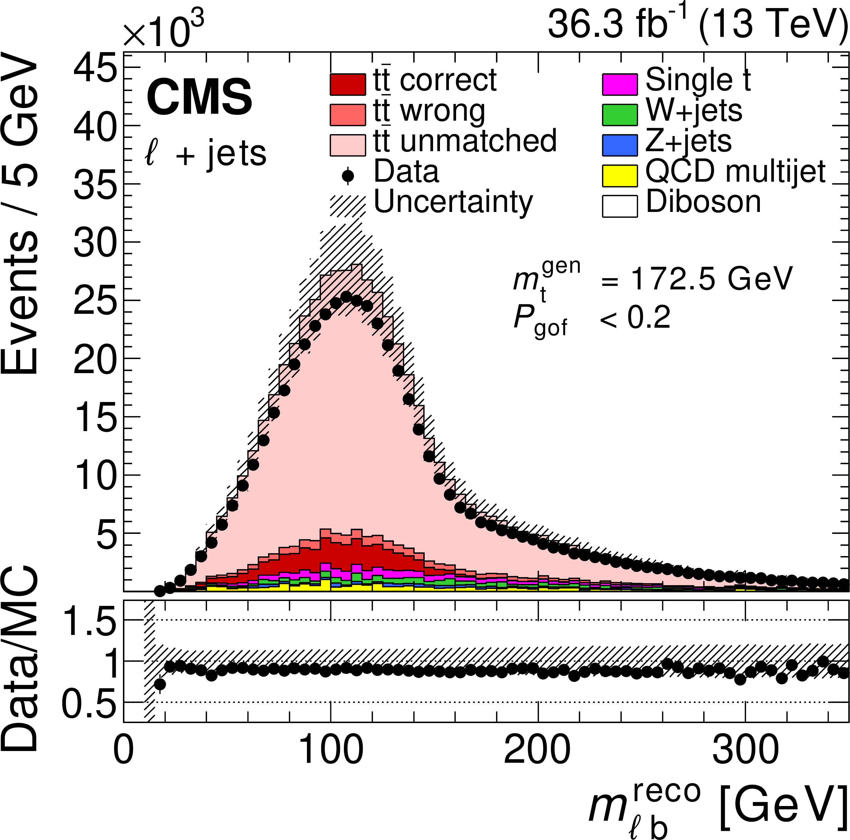
The distributions of the top quark mass from the kinematic fit for the $ P_{\text{gof}} > $ 0.2 category (left) and of the invariant mass of the lepton and the jet assigned to the top quark decaying in the lepton+jets channel for the $ P_{\text{gof}} < $ 0.2 category (right). Data are shown as points with vertical error bars showing the statistical uncertainties. The coloured histograms show the simulated signal and background contributions. The simulated signal is decomposed into the contributions from correct, wrong, or unmatched permutations, as introduced in Section 2.3. The uncertainty bands contain statistical uncertainties in the simulation, normalisation uncertainties due to the integrated luminosity and cross section, JES correction, and all uncertainties that are evaluated from event-based weights. A large part of the depicted uncertainties in the expected event yields are correlated. The lower panels show the ratio of data to the prediction. In the figures, the default value of $ m_{\mathrm{t}}^\text{gen}= $ 172.5 GeV is used. Figures taken from Ref. [71]. |
png pdf |
Figure 21-a:
The distributions of the top quark mass from the kinematic fit for the $ P_{\text{gof}} > $ 0.2 category (left) and of the invariant mass of the lepton and the jet assigned to the top quark decaying in the lepton+jets channel for the $ P_{\text{gof}} < $ 0.2 category (right). Data are shown as points with vertical error bars showing the statistical uncertainties. The coloured histograms show the simulated signal and background contributions. The simulated signal is decomposed into the contributions from correct, wrong, or unmatched permutations, as introduced in Section 2.3. The uncertainty bands contain statistical uncertainties in the simulation, normalisation uncertainties due to the integrated luminosity and cross section, JES correction, and all uncertainties that are evaluated from event-based weights. A large part of the depicted uncertainties in the expected event yields are correlated. The lower panels show the ratio of data to the prediction. In the figures, the default value of $ m_{\mathrm{t}}^\text{gen}= $ 172.5 GeV is used. Figures taken from Ref. [71]. |
png pdf |
Figure 21-b:
The distributions of the top quark mass from the kinematic fit for the $ P_{\text{gof}} > $ 0.2 category (left) and of the invariant mass of the lepton and the jet assigned to the top quark decaying in the lepton+jets channel for the $ P_{\text{gof}} < $ 0.2 category (right). Data are shown as points with vertical error bars showing the statistical uncertainties. The coloured histograms show the simulated signal and background contributions. The simulated signal is decomposed into the contributions from correct, wrong, or unmatched permutations, as introduced in Section 2.3. The uncertainty bands contain statistical uncertainties in the simulation, normalisation uncertainties due to the integrated luminosity and cross section, JES correction, and all uncertainties that are evaluated from event-based weights. A large part of the depicted uncertainties in the expected event yields are correlated. The lower panels show the ratio of data to the prediction. In the figures, the default value of $ m_{\mathrm{t}}^\text{gen}= $ 172.5 GeV is used. Figures taken from Ref. [71]. |
png pdf |
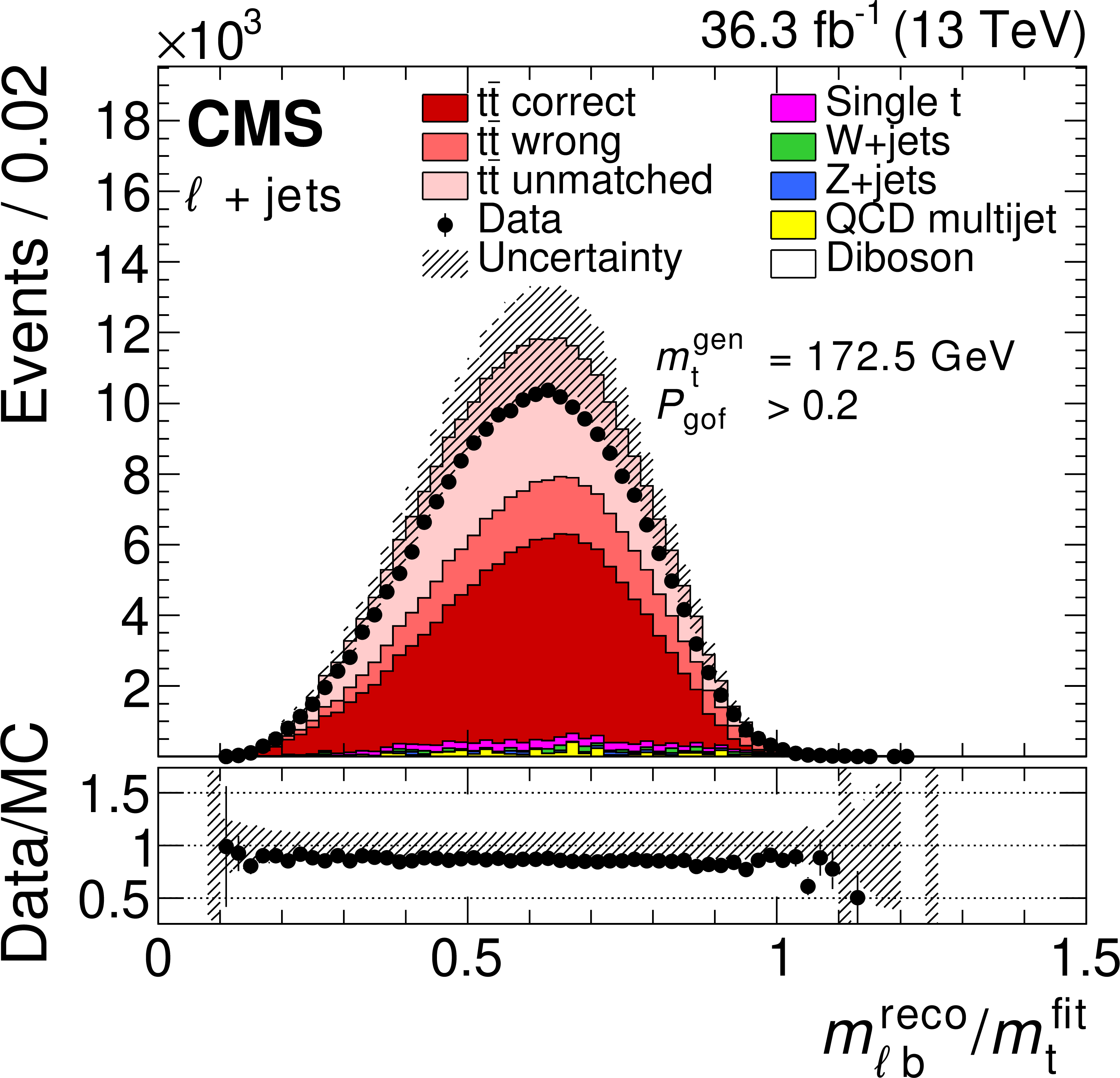
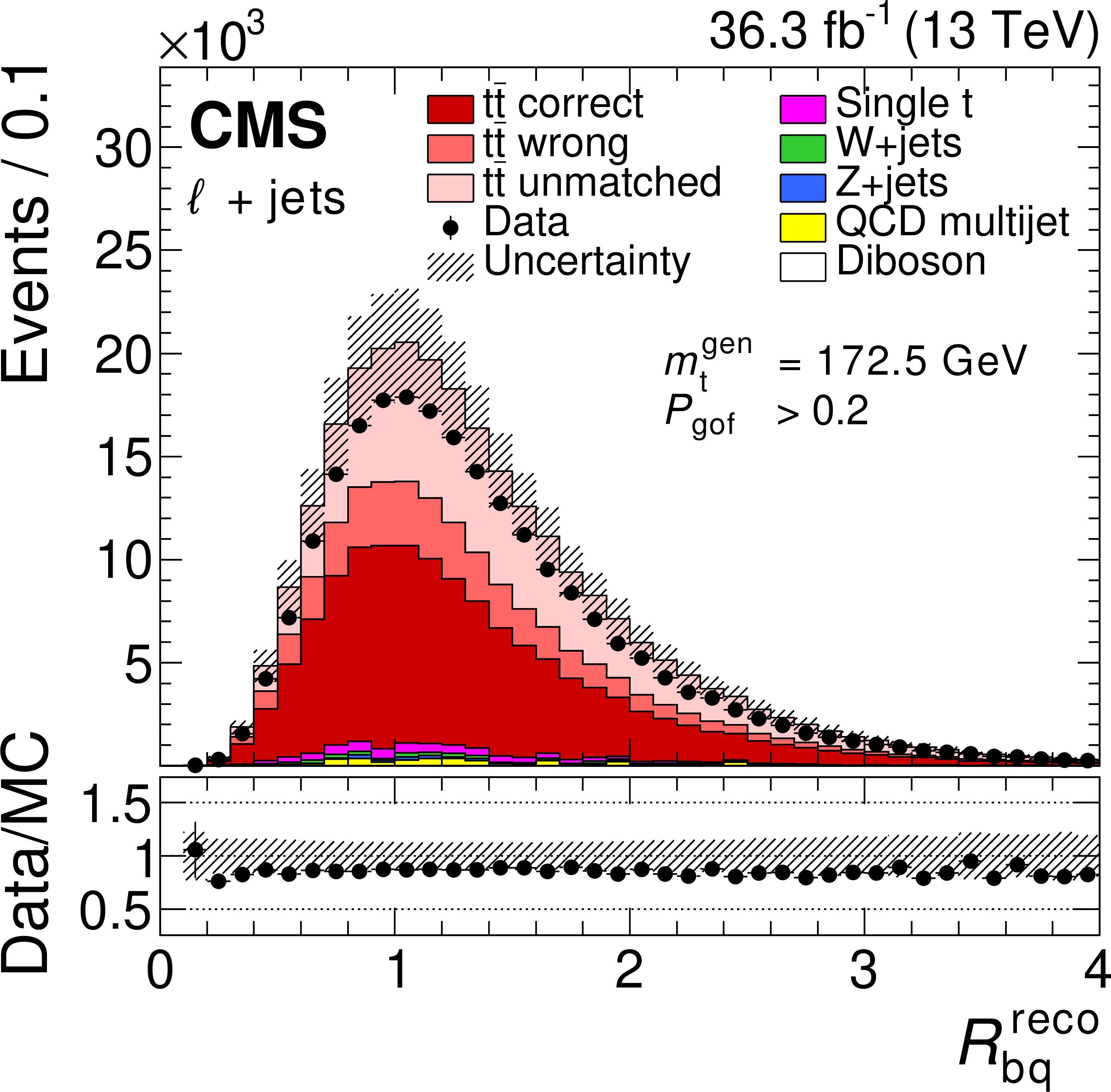
Figure 22:
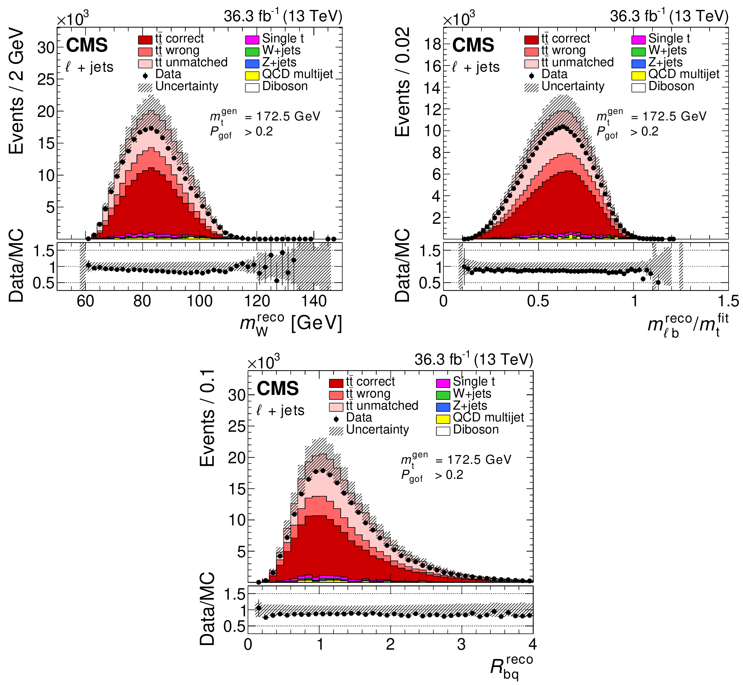
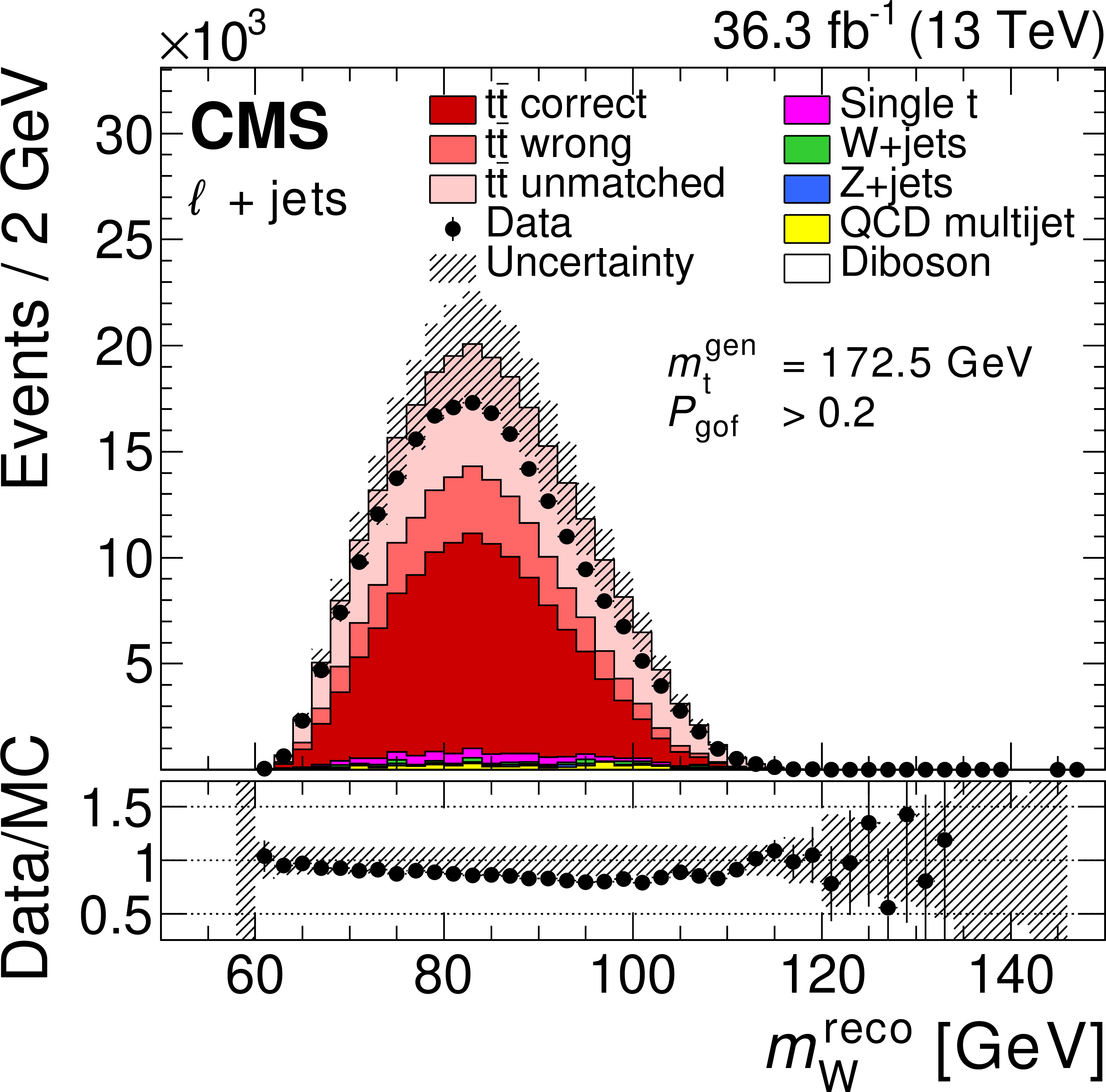
The distributions of $ m_{\mathrm{W}}^\text{reco} $ (upper left), $ m_{\ell\mathrm{b}}^\text{reco}/m_{\mathrm{t}}^\text{fit} $ (upper right), and $ R_{\mathrm{b}\mathrm{q}}^\text{reco} $ (lower) for the $ P_{\text{gof}} > $ 0.2 category. Symbols and patterns are the same as in Fig. 21. In the figures, the default value of $ m_{\mathrm{t}}^\text{gen}= $ 172.5 GeV is used. Figures taken from Ref. [71]. |
png pdf |
Figure 22-a:
The distributions of $ m_{\mathrm{W}}^\text{reco} $ (upper left), $ m_{\ell\mathrm{b}}^\text{reco}/m_{\mathrm{t}}^\text{fit} $ (upper right), and $ R_{\mathrm{b}\mathrm{q}}^\text{reco} $ (lower) for the $ P_{\text{gof}} > $ 0.2 category. Symbols and patterns are the same as in Fig. 21. In the figures, the default value of $ m_{\mathrm{t}}^\text{gen}= $ 172.5 GeV is used. Figures taken from Ref. [71]. |
png pdf |
Figure 22-b:
The distributions of $ m_{\mathrm{W}}^\text{reco} $ (upper left), $ m_{\ell\mathrm{b}}^\text{reco}/m_{\mathrm{t}}^\text{fit} $ (upper right), and $ R_{\mathrm{b}\mathrm{q}}^\text{reco} $ (lower) for the $ P_{\text{gof}} > $ 0.2 category. Symbols and patterns are the same as in Fig. 21. In the figures, the default value of $ m_{\mathrm{t}}^\text{gen}= $ 172.5 GeV is used. Figures taken from Ref. [71]. |
png pdf |
Figure 22-c:
The distributions of $ m_{\mathrm{W}}^\text{reco} $ (upper left), $ m_{\ell\mathrm{b}}^\text{reco}/m_{\mathrm{t}}^\text{fit} $ (upper right), and $ R_{\mathrm{b}\mathrm{q}}^\text{reco} $ (lower) for the $ P_{\text{gof}} > $ 0.2 category. Symbols and patterns are the same as in Fig. 21. In the figures, the default value of $ m_{\mathrm{t}}^\text{gen}= $ 172.5 GeV is used. Figures taken from Ref. [71]. |
png pdf |
Figure 23:
Comparison of the expected total uncertainty in $ m_{\mathrm{t}} $ in the combined lepton+jets channel and for different observable categories defined in Table 4. Figure taken from Ref. [71]. |
png pdf |
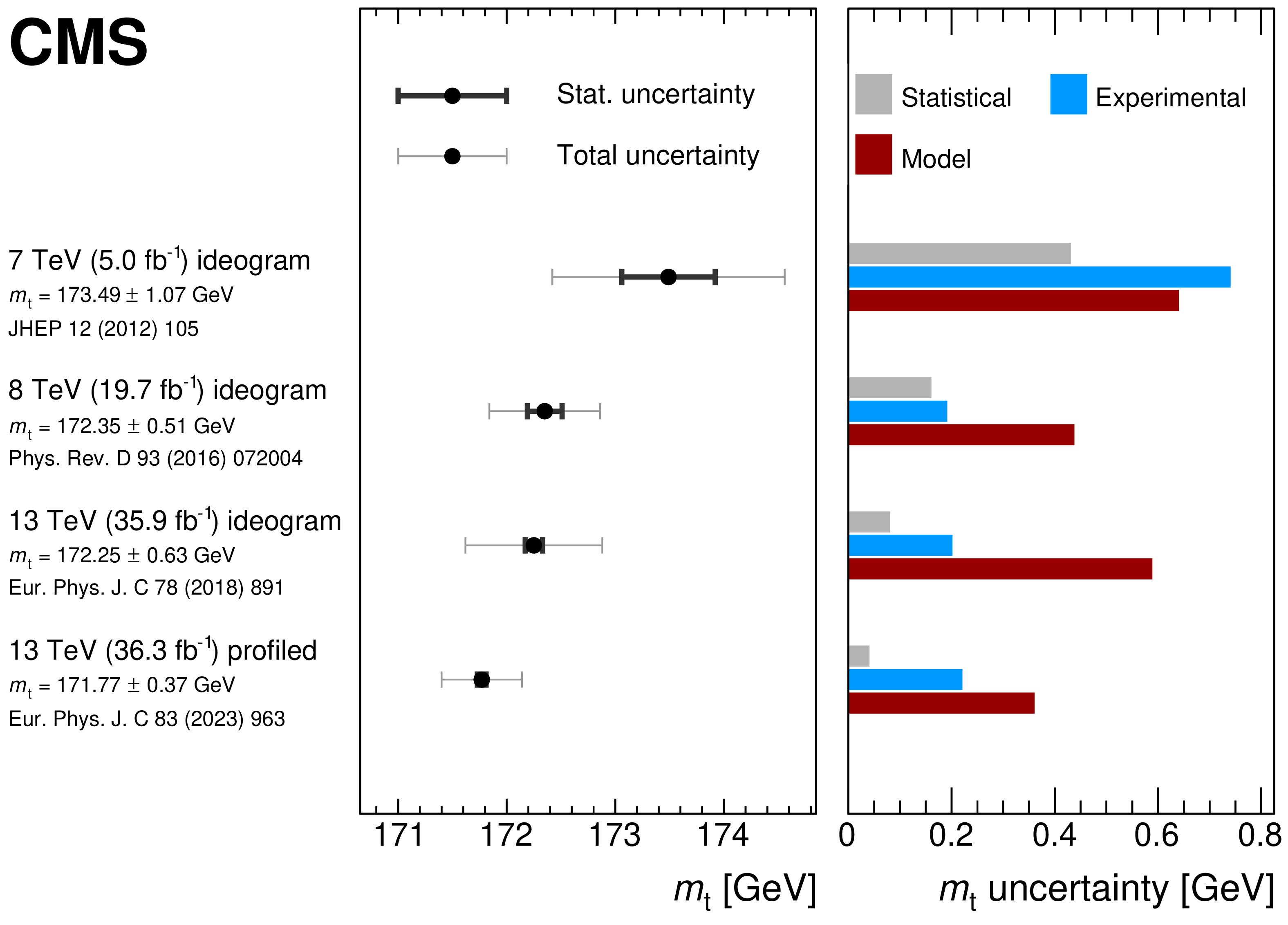
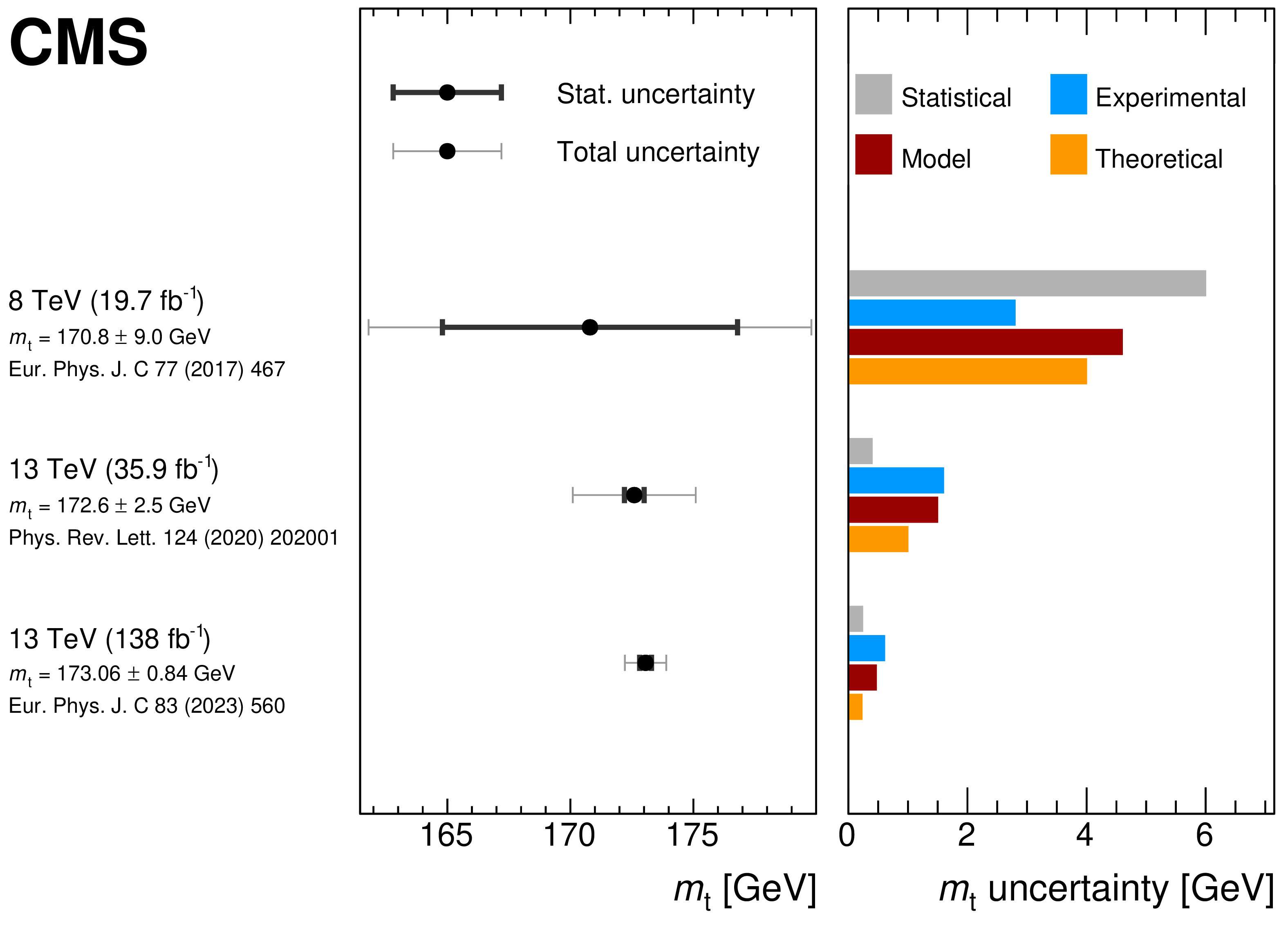
Figure 24:
Summary of the direct $ m_{\mathrm{t}} $ measurements in the lepton+jets channel by the CMS Collaboration. The left panel shows the measured value of $ m_{\mathrm{t}} $ (marker) with statistical (black bars) and total (grey bars) uncertainties. The right panel displays a breakdown of contributing uncertainty groups and their impact on the uncertainty in the measurement. The two results at 13 TeV are derived from the same data. The figure is compiled from Refs. [48,53,61,71]. |

png pdf |
Figure 25:
Comparison of the CMS direct $ m_{\mathrm{t}} $ measurements from the Run-2 data collected in 2016 at $ \sqrt{s} = $ 13 TeV to the best Run-1 measurements at $ \sqrt{s} = $ 8 TeV in each channel. The horizontal bars display the total uncertainty in the measurements and the red band shows the uncertainty in the Run-1 combination [72]. The figure is compiled from Refs. [53,61,71,60,63,69,62,72]. |

png pdf |
Figure 26:
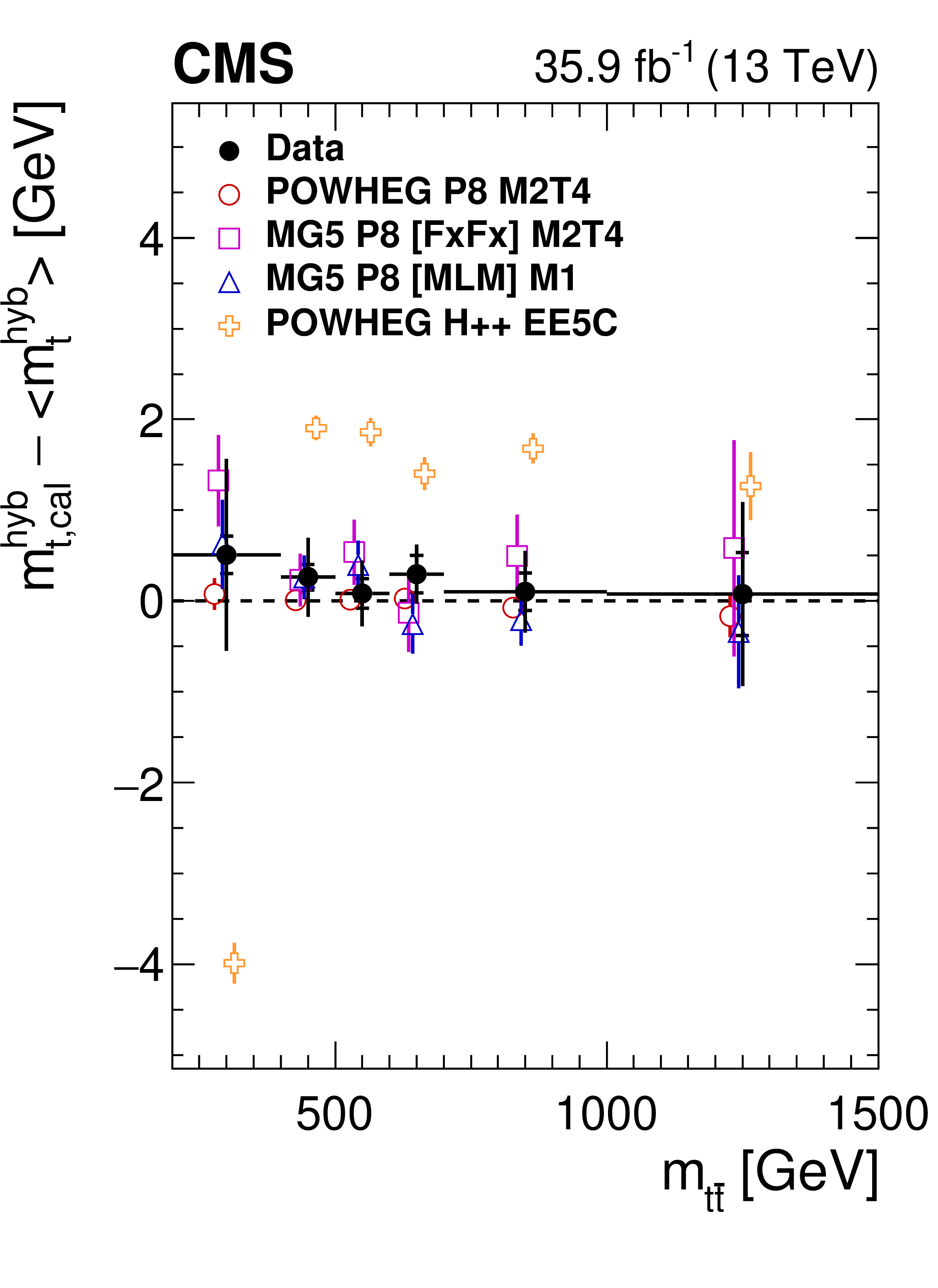
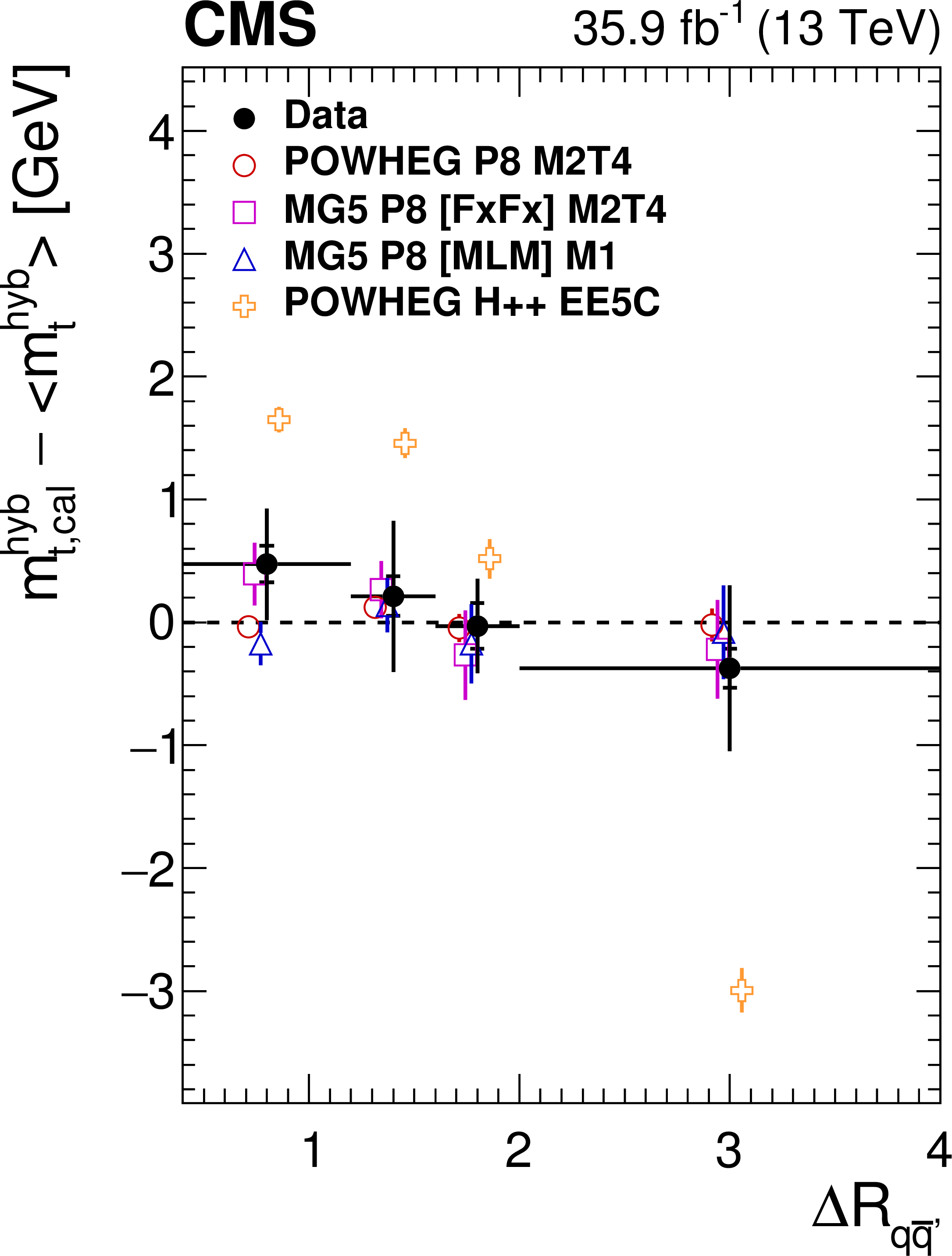
Difference of the $ m_{\mathrm{t}} $ extracted after calibration in each bin and from the inclusive sample as a function of the invariant mass of the $ \mathrm{t} \overline{\mathrm{t}} $ system $ m_{{\mathrm{t}\overline{\mathrm{t}}} } $ (left) and the $ \Delta R $ between the light-quark jets $ \Delta R_{\mathrm{q}{\overline{\mathrm{q}}{\prime}} } $ (right), obtained from the hybrid fit [61], compared to different generator models. The filled circles represent the data, and the other symbols are for the simulations. For reasons of clarity, the horizontal bars indicating the bin widths are shown only for the data points and each of the simulations is shown as a single offset point with a vertical error bar representing its statistical uncertainty. The statistical uncertainty of the data is displayed by the inner error bars. For the outer error bars, the systematic uncertainties are added in quadrature. Figures taken from Ref. [61]. |
png pdf |
Figure 26-a:
Difference of the $ m_{\mathrm{t}} $ extracted after calibration in each bin and from the inclusive sample as a function of the invariant mass of the $ \mathrm{t} \overline{\mathrm{t}} $ system $ m_{{\mathrm{t}\overline{\mathrm{t}}} } $ (left) and the $ \Delta R $ between the light-quark jets $ \Delta R_{\mathrm{q}{\overline{\mathrm{q}}{\prime}} } $ (right), obtained from the hybrid fit [61], compared to different generator models. The filled circles represent the data, and the other symbols are for the simulations. For reasons of clarity, the horizontal bars indicating the bin widths are shown only for the data points and each of the simulations is shown as a single offset point with a vertical error bar representing its statistical uncertainty. The statistical uncertainty of the data is displayed by the inner error bars. For the outer error bars, the systematic uncertainties are added in quadrature. Figures taken from Ref. [61]. |
png pdf |
Figure 26-b:
Difference of the $ m_{\mathrm{t}} $ extracted after calibration in each bin and from the inclusive sample as a function of the invariant mass of the $ \mathrm{t} \overline{\mathrm{t}} $ system $ m_{{\mathrm{t}\overline{\mathrm{t}}} } $ (left) and the $ \Delta R $ between the light-quark jets $ \Delta R_{\mathrm{q}{\overline{\mathrm{q}}{\prime}} } $ (right), obtained from the hybrid fit [61], compared to different generator models. The filled circles represent the data, and the other symbols are for the simulations. For reasons of clarity, the horizontal bars indicating the bin widths are shown only for the data points and each of the simulations is shown as a single offset point with a vertical error bar representing its statistical uncertainty. The statistical uncertainty of the data is displayed by the inner error bars. For the outer error bars, the systematic uncertainties are added in quadrature. Figures taken from Ref. [61]. |

png pdf |
Figure 27:
Feynman diagrams of the $ t $-channel single top quark production at LO corresponding to five- (left) and four-flavour (right) schemes, assuming five (u, d, s, c, b) or four (u, d, s, c) active quark flavours in the proton, respectively. At NLO in perturbative QCD, the right diagram is also part of the five-flavour scheme. |

png pdf |
Figure 27-a:
Feynman diagrams of the $ t $-channel single top quark production at LO corresponding to five- (left) and four-flavour (right) schemes, assuming five (u, d, s, c, b) or four (u, d, s, c) active quark flavours in the proton, respectively. At NLO in perturbative QCD, the right diagram is also part of the five-flavour scheme. |

png pdf |
Figure 27-b:
Feynman diagrams of the $ t $-channel single top quark production at LO corresponding to five- (left) and four-flavour (right) schemes, assuming five (u, d, s, c, b) or four (u, d, s, c) active quark flavours in the proton, respectively. At NLO in perturbative QCD, the right diagram is also part of the five-flavour scheme. |
png pdf |
Figure 28:
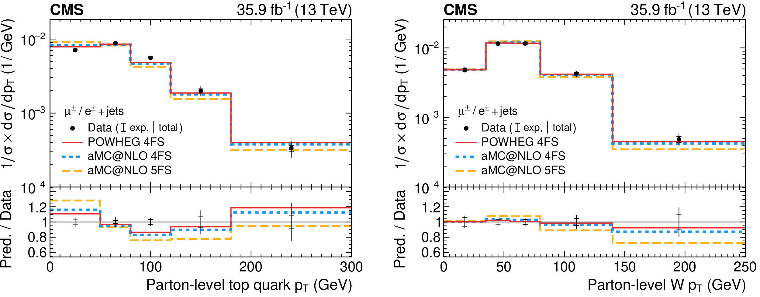
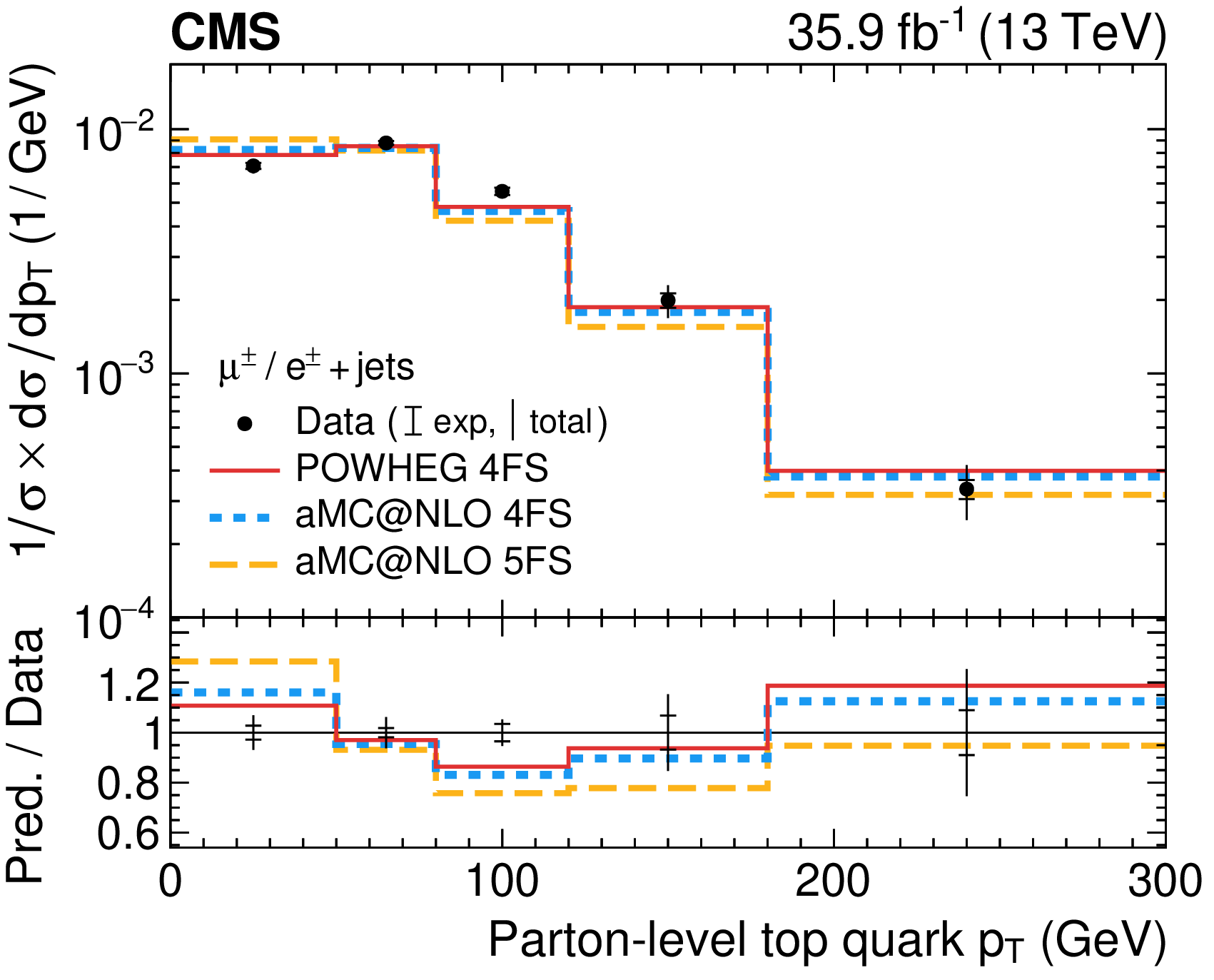
Normalised differential cross section of the $ t $-channel single top quark production as a function of the $ p_{\mathrm{T}} $ of the parton-level top quark (left) and the W boson (right). Figures taken from Ref. [204]. |
png pdf |
Figure 28-a:
Normalised differential cross section of the $ t $-channel single top quark production as a function of the $ p_{\mathrm{T}} $ of the parton-level top quark (left) and the W boson (right). Figures taken from Ref. [204]. |

png pdf |
Figure 28-b:
Normalised differential cross section of the $ t $-channel single top quark production as a function of the $ p_{\mathrm{T}} $ of the parton-level top quark (left) and the W boson (right). Figures taken from Ref. [204]. |
png pdf |
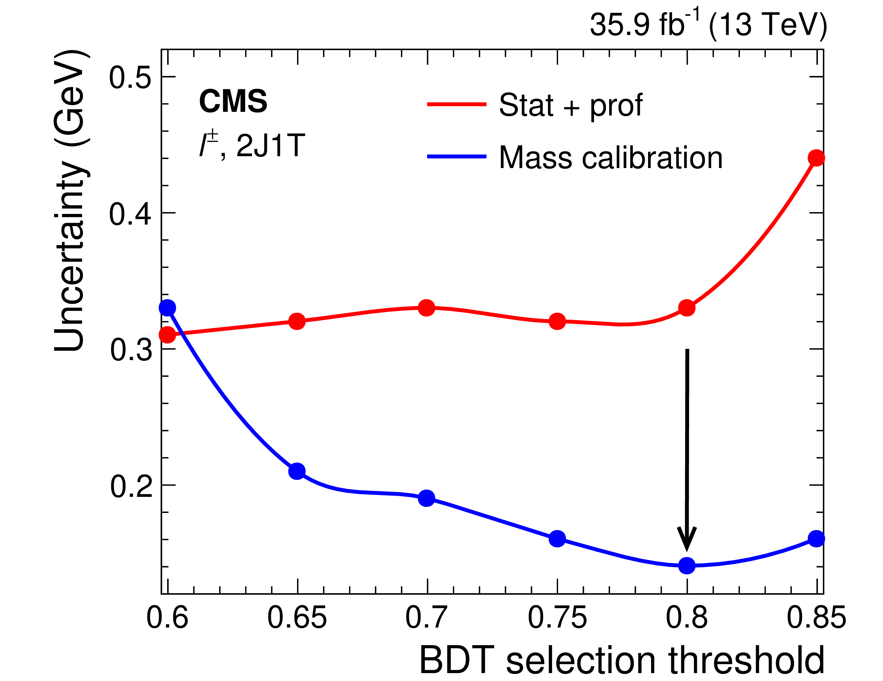
Figure 29:
The uncertainty in $ m_{\mathrm{t}} $ from the statistical and profiled systematic components (red) and uncertainty in the $ m_{\mathrm{t}} $ calibration (blue) as a function of the cutoff on the BDT score. Figure taken from Ref. [67]. |

png pdf |
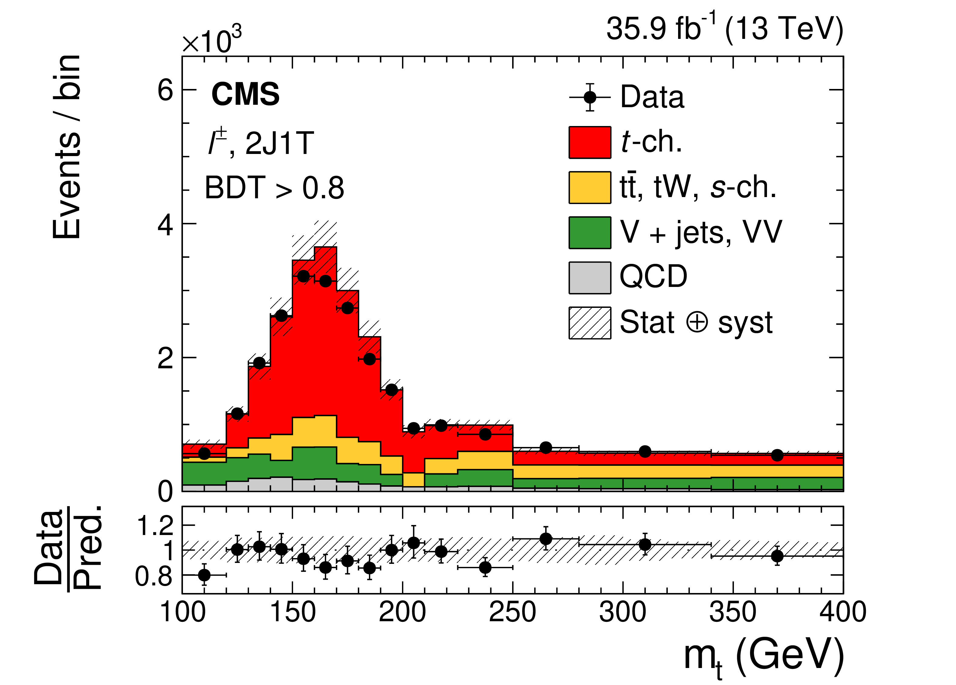
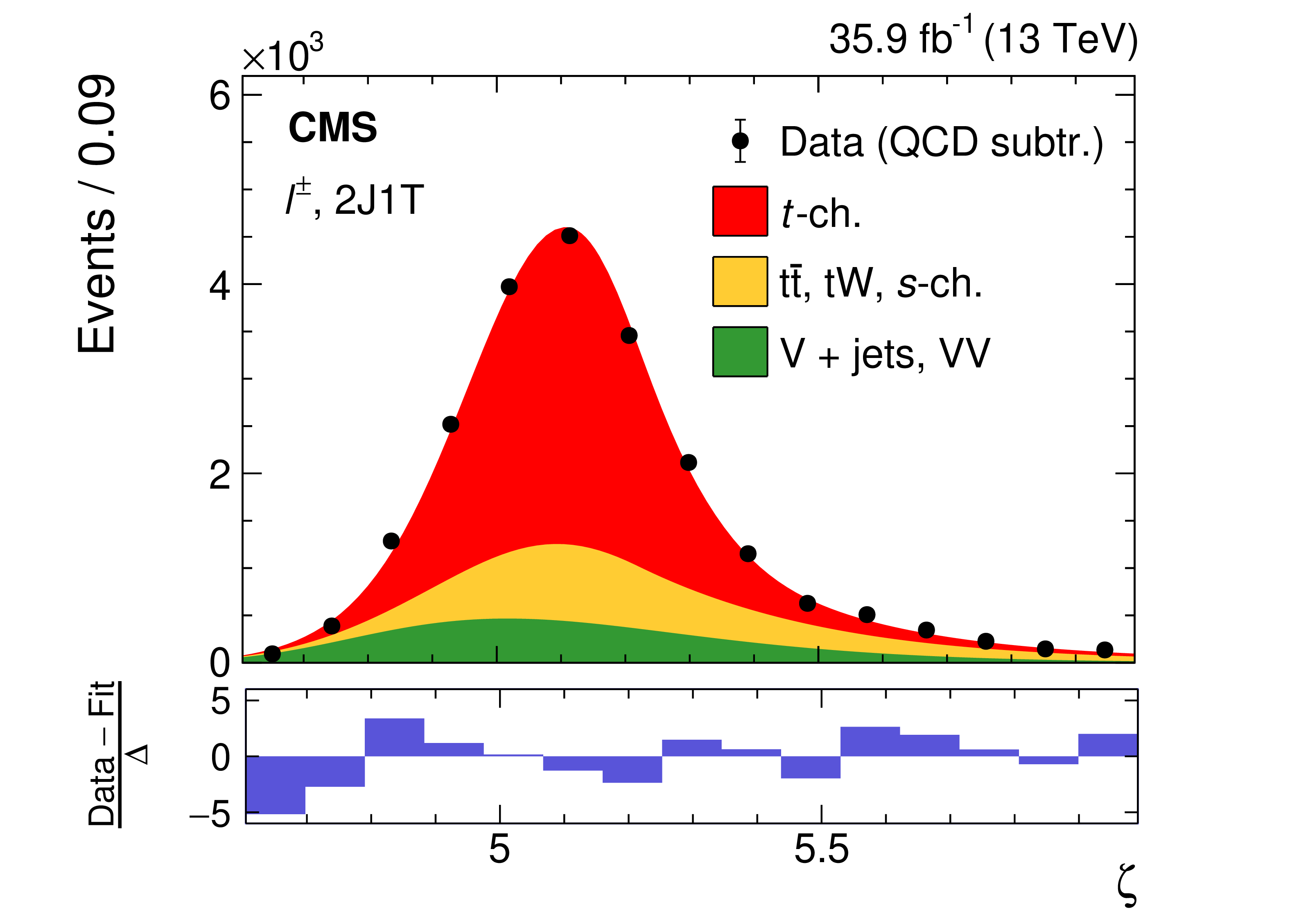
Figure 30:
Data-to-simulation comparison of the reconstructed top quark mass (left) and postfit $ \zeta=\ln(m_{\mathrm{t}}/$ 1 GeV (right) distributions after BDT selection. The lower panel in the left plot shows the data-to-simulation ratios for each bin, while the lower panel in the right plot shows the normalised residuals or pulls, determined using the bin contents of the data distributions (after background QCD subtraction) and the $ F(\zeta) $ values evaluated at the centre of the bins. Figures taken from Ref. [67]. |
png pdf |
Figure 30-a:
Data-to-simulation comparison of the reconstructed top quark mass (left) and postfit $ \zeta=\ln(m_{\mathrm{t}}/$ 1 GeV (right) distributions after BDT selection. The lower panel in the left plot shows the data-to-simulation ratios for each bin, while the lower panel in the right plot shows the normalised residuals or pulls, determined using the bin contents of the data distributions (after background QCD subtraction) and the $ F(\zeta) $ values evaluated at the centre of the bins. Figures taken from Ref. [67]. |
png pdf |
Figure 30-b:
Data-to-simulation comparison of the reconstructed top quark mass (left) and postfit $ \zeta=\ln(m_{\mathrm{t}}/$ 1 GeV (right) distributions after BDT selection. The lower panel in the left plot shows the data-to-simulation ratios for each bin, while the lower panel in the right plot shows the normalised residuals or pulls, determined using the bin contents of the data distributions (after background QCD subtraction) and the $ F(\zeta) $ values evaluated at the centre of the bins. Figures taken from Ref. [67]. |
png pdf |
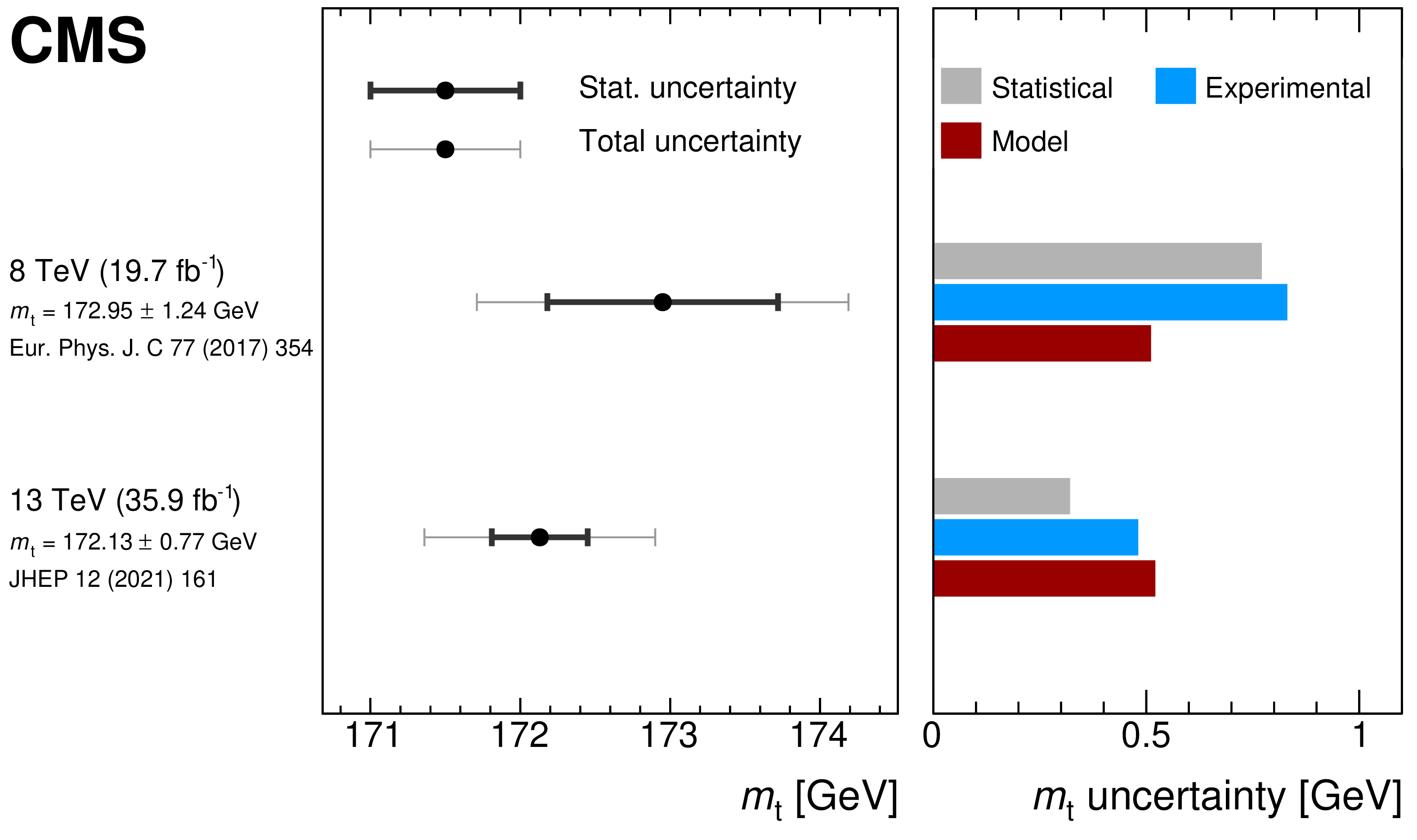
Figure 31:
Summary of $ m_{\mathrm{t}} $ measurements in single top quark events. The left panel shows the measured value of $ m_{\mathrm{t}} $ (marker) with statistical (thick bars) and total (thin bars) uncertainties. In the case of the 13 TeV measurement [67], the statistical component of the uncertainty includes contributions from the statistical and profiled systematic uncertainties. The right panel displays a breakdown of contributing uncertainty groups and their impact on the uncertainty in the measurement. The figure is compiled from Refs. [58,67]. |
png pdf |
Figure 32:
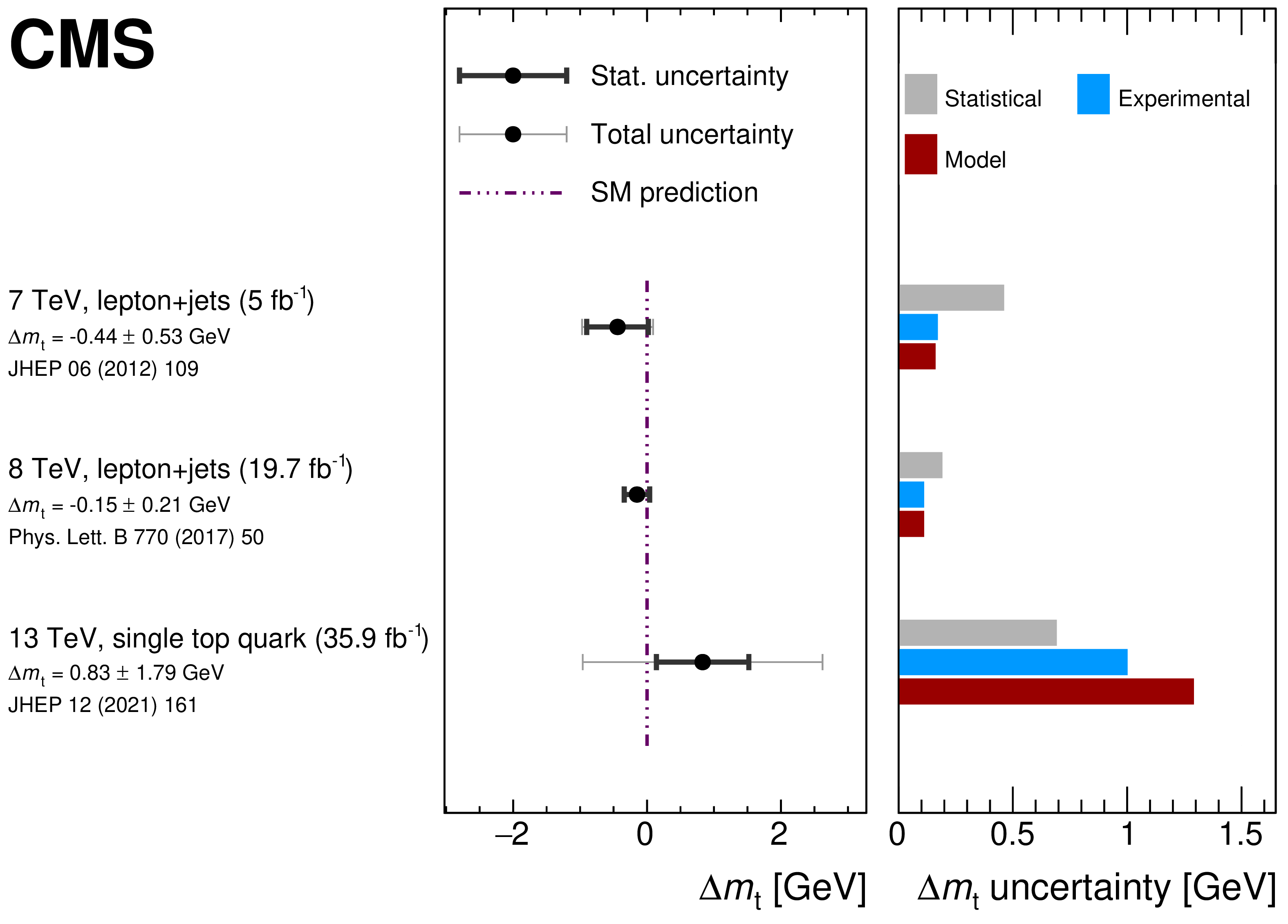
Summary of $ \Delta m_{\mathrm{t}} $ measurements in $ \mathrm{t} \overline{\mathrm{t}} $ and single top quark events. The left panel shows the measured value of $ \Delta m_{\mathrm{t}} $ (marker) with statistical (thick bars) and total (thin bars) uncertainties. In the case of the single top quark measurement [67], the statistical component of the uncertainty includes contributions from the statistical and profiled systematic uncertainties. The right panel displays a breakdown of contributing uncertainty groups and their impact on the uncertainty in the measurement. The figure is compiled from Refs. [209,210,67]. |
png pdf |
Figure 33:
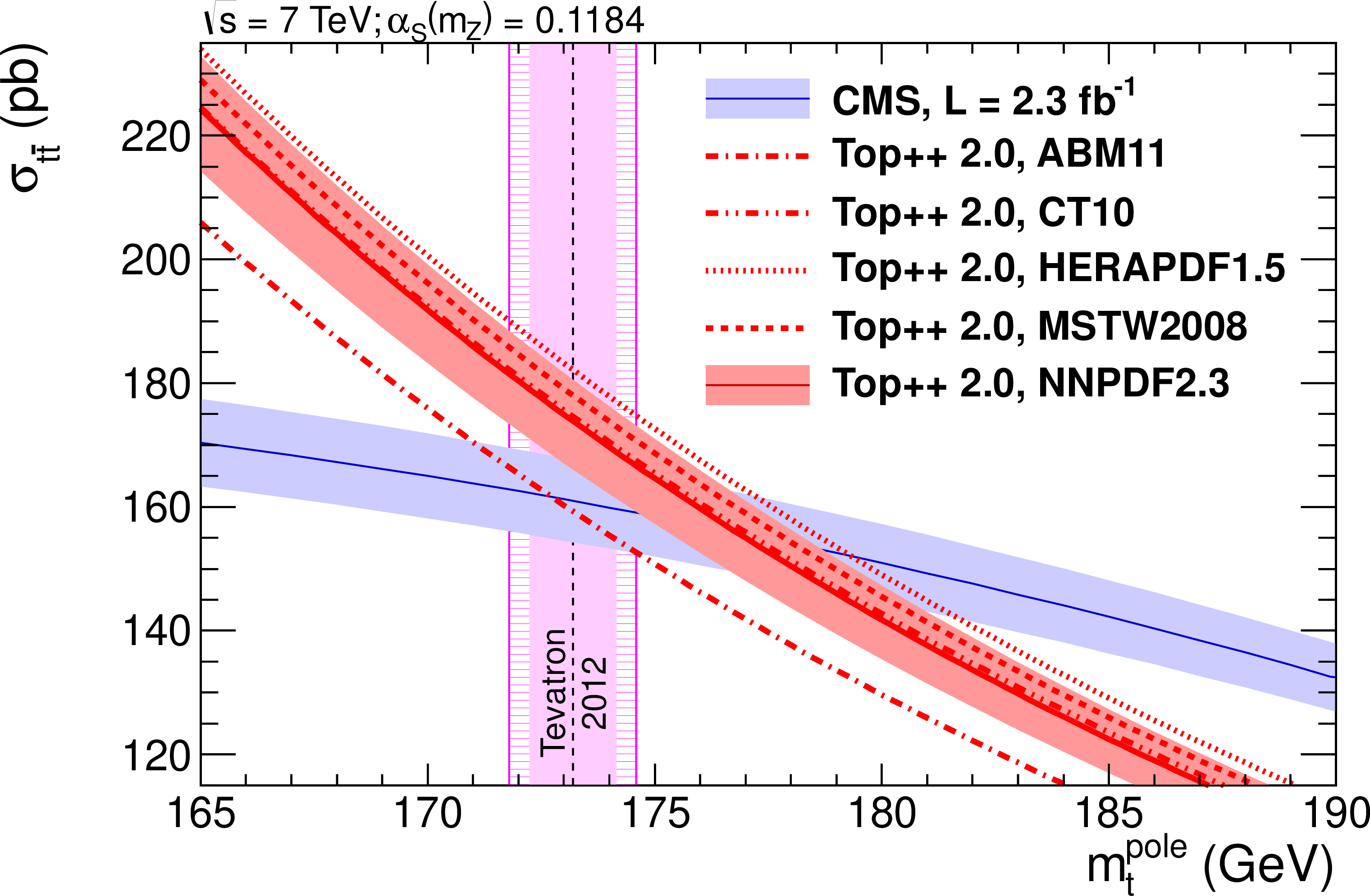
Predicted $ \sigma_{{\mathrm{t}\overline{\mathrm{t}}} } $ as a function of the top quark pole mass, using different PDF sets (red shaded band and red lines of different styles), compared to the cross section measured by CMS assuming $ m_{\mathrm{t}}^{\text{MC}}=m_{\mathrm{t}}^{\text{pole}} $ (blue shaded band). The uncertainties in the measured $ \sigma_{{\mathrm{t}\overline{\mathrm{t}}} } $ as well as the scale and PDF uncertainties in the prediction with NNPDF-2.3 [126] are illustrated by the filled band. The $ m_{\mathrm{t}}^{\text{MC}} $ result obtained in direct measurements to that date is shown as hatched area. The inner (solid) area of the vertical band corresponds to the quoted experimental uncertainty in $ m_{\mathrm{t}}^{\text{MC}} $, while the outer (hatched) area additionally accounts for a possible difference between this value and $ m_{\mathrm{t}}^{\text{pole}} $. Figure taken from Ref. [52]. |

png pdf |
Figure 34:
Values of $ m_{\mathrm{t}}^{\text{pole}} $ obtained by using measured $ \sigma_{{\mathrm{t}\overline{\mathrm{t}}} } $ together with the prediction at NNLO+NNLL using different NNLO PDF sets. The filled symbols represent the results obtained when using the world average of $ \alpha_\mathrm{S}(m_{\mathrm{Z}}) $, while the open symbols indicate the results obtained with the default $ \alpha_\mathrm{S}(m_{\mathrm{Z}}) $ value of the respective PDF set. The inner error bars include the uncertainties in the measured cross section and in the LHC beam energy, as well as the PDF and scale uncertainties in the predicted cross section. The outer error bars additionally account for the uncertainty in the $ \alpha_\mathrm{S}(m_{\mathrm{Z}}) $ value used for a specific prediction. For comparison, the most precise $ m_{\mathrm{t}}^{\text{MC}} $ to that date is shown as vertical band, where the inner (solid) area corresponds to the original uncertainty of the direct $ m_{\mathrm{t}} $ average, while the outer (hatched) area additionally accounts for the possible difference between $ m_{\mathrm{t}}^{\text{MC}} $ and $ m_{\mathrm{t}}^{\text{pole}} $. Figure taken from Ref. [52]. |

png pdf |
Figure 35:
Likelihood for the predicted dependence of $ \sigma_{{\mathrm{t}\overline{\mathrm{t}}} } $ on $ m_{\mathrm{t}}^{\text{pole}} $ for 7 and 8 TeV determined with TOP++, using the NNPDF-3.0 PDF set. The measured dependencies on the mass are given by the dashed lines, their 1 $ \sigma $ uncertainties are represented by the dotted lines. The extracted mass at each value of $ \sqrt{s} $ is indicated by a black point, with its $ \pm $ 1 standard deviation uncertainty constructed from the continuous contour, corresponding to $ -2\Delta\log(L_{\text{pred}}L_{\text{exp}})= $ 1. Figure taken from Ref. [54]. |
png pdf |
Figure 36:
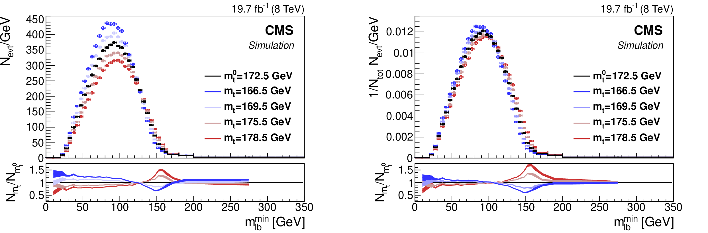
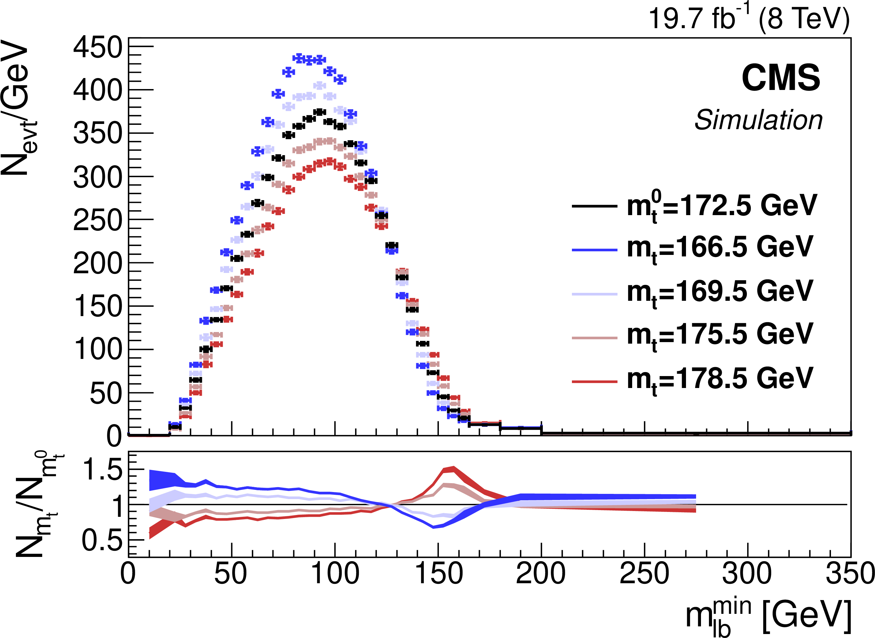
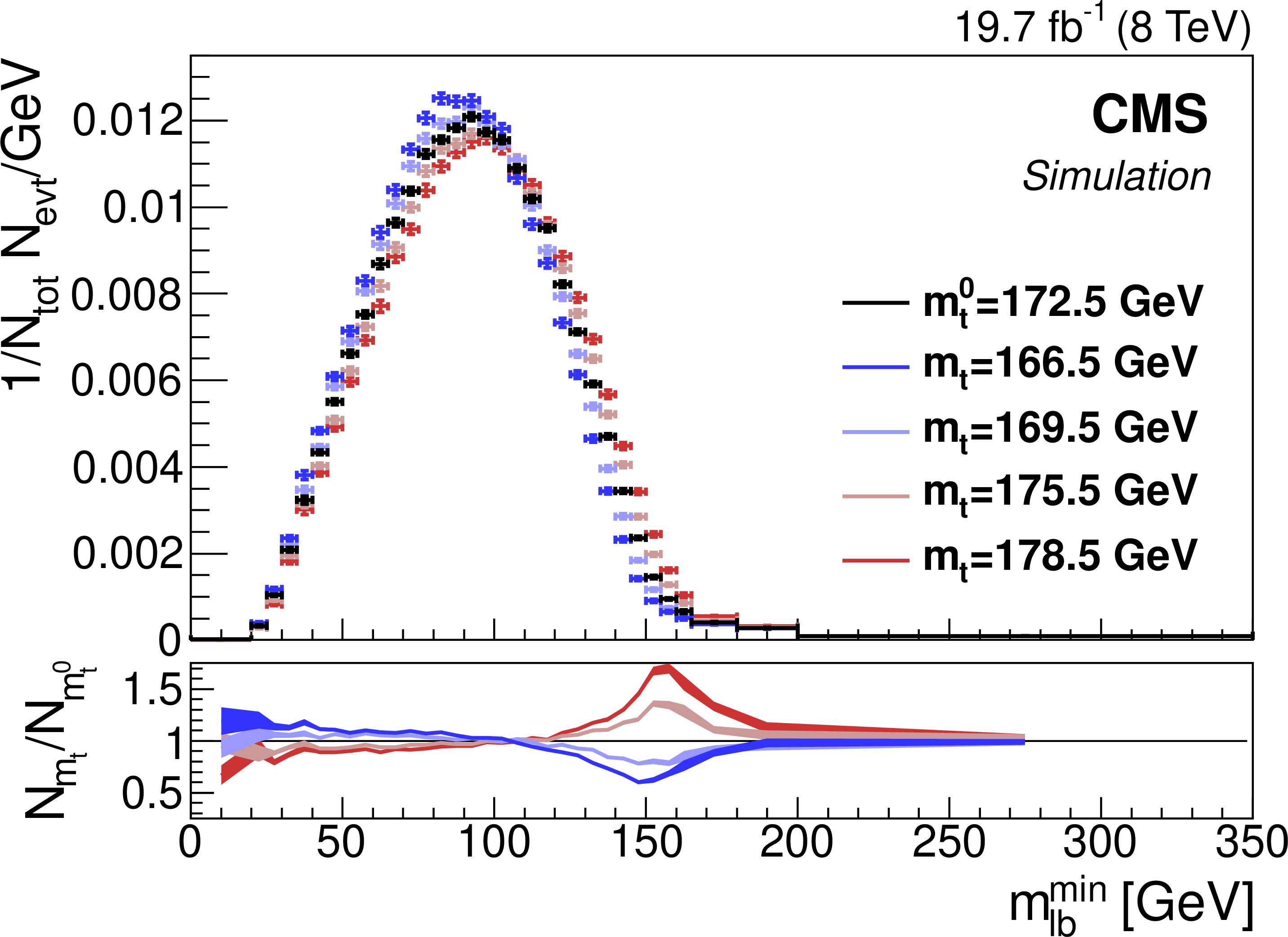
Absolute (left) and shape (right) distributions of $ m_{\ell\mathrm{b}}^\text{min} $ for $ \mathrm{t} \overline{\mathrm{t}} $ production at the LHC at $ \sqrt{s} = $ 8 TeV after detector simulation and event selection in the $ \mathrm{e}\mu $ channel. The central prediction (black symbols) is obtained at the value of $ m_{\mathrm{t}}^{\text{MC}} $ of 172.5 GeV, denoted as $ m_{\mathrm{t}}^0 $. Predictions assuming different $ m_{\mathrm{t}}^{\text{MC}} $ values are shown by different colours. |
png pdf |
Figure 36-a:
Absolute (left) and shape (right) distributions of $ m_{\ell\mathrm{b}}^\text{min} $ for $ \mathrm{t} \overline{\mathrm{t}} $ production at the LHC at $ \sqrt{s} = $ 8 TeV after detector simulation and event selection in the $ \mathrm{e}\mu $ channel. The central prediction (black symbols) is obtained at the value of $ m_{\mathrm{t}}^{\text{MC}} $ of 172.5 GeV, denoted as $ m_{\mathrm{t}}^0 $. Predictions assuming different $ m_{\mathrm{t}}^{\text{MC}} $ values are shown by different colours. |
png pdf |
Figure 36-b:
Absolute (left) and shape (right) distributions of $ m_{\ell\mathrm{b}}^\text{min} $ for $ \mathrm{t} \overline{\mathrm{t}} $ production at the LHC at $ \sqrt{s} = $ 8 TeV after detector simulation and event selection in the $ \mathrm{e}\mu $ channel. The central prediction (black symbols) is obtained at the value of $ m_{\mathrm{t}}^{\text{MC}} $ of 172.5 GeV, denoted as $ m_{\mathrm{t}}^0 $. Predictions assuming different $ m_{\mathrm{t}}^{\text{MC}} $ values are shown by different colours. |
png pdf |
Figure 37:
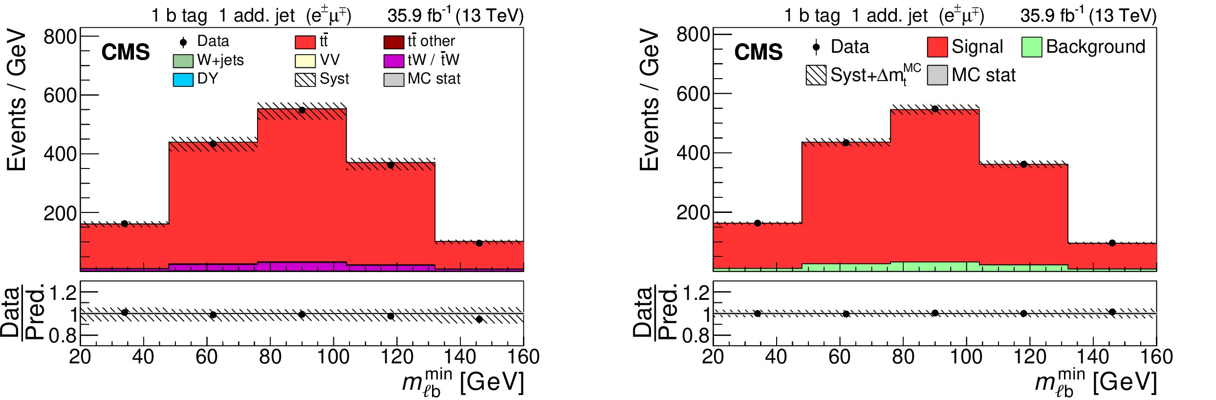
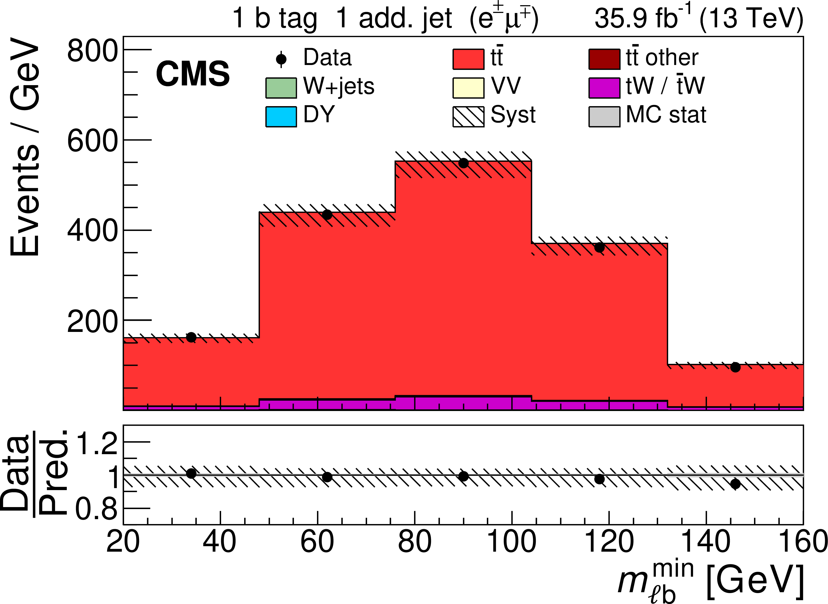
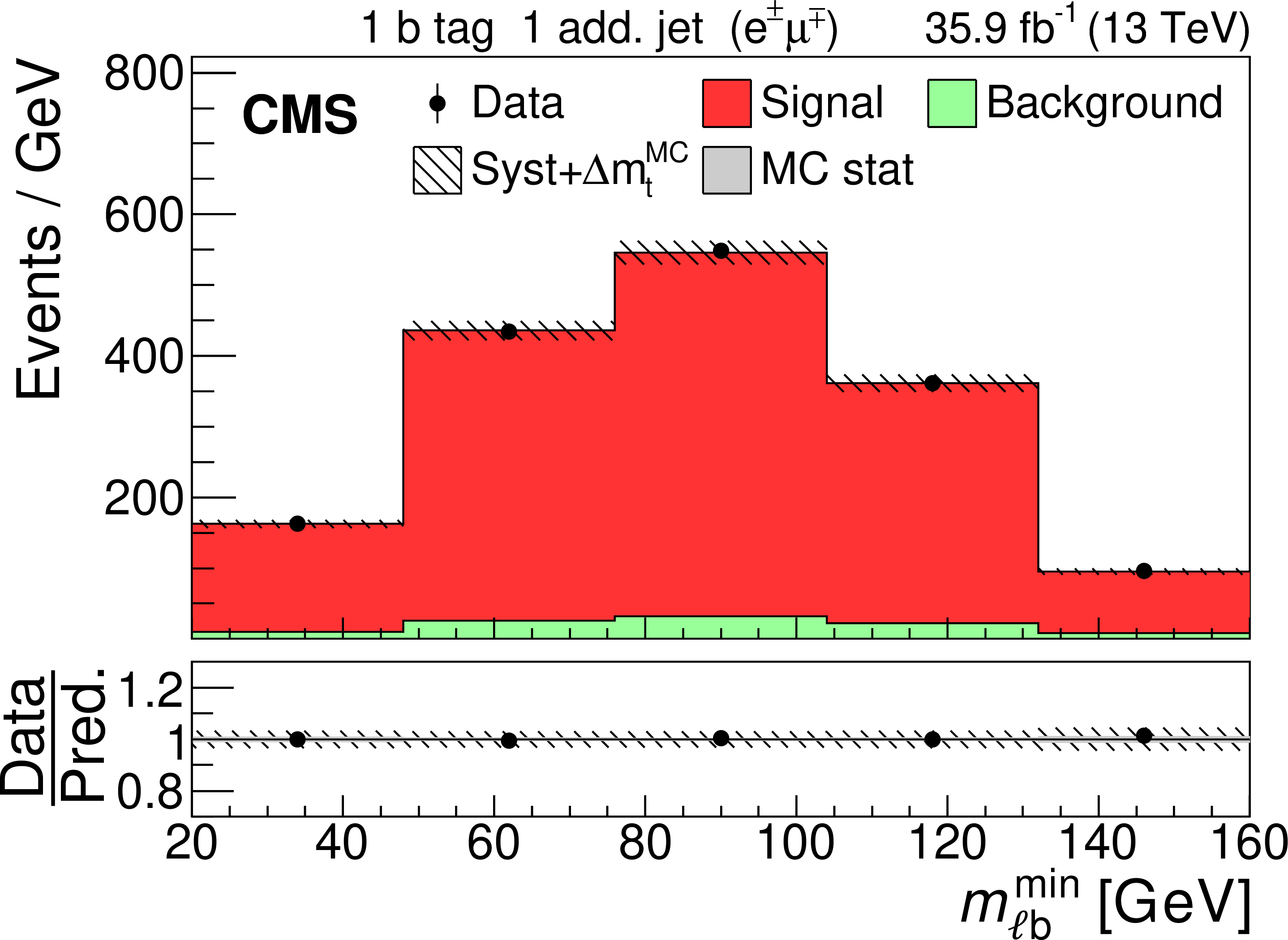
Data (points) compared to pre-fit (left) and post-fit (right) $ m_{\ell\mathrm{b}}^\text{min} $ distributions of the expected signal and backgrounds from simulation (shaded histograms) used in the simultaneous fit of $ \sigma_{{\mathrm{t}\overline{\mathrm{t}}} } $ and $ m_{\mathrm{t}}^{\text{MC}} $. Events with exactly one b-tagged jets are shown. The hatched bands correspond to the total uncertainty in the sum of the predicted yields. The ratios of data to the sum of the predicted yields are shown in the lower panel. Here, the solid grey band represents the contribution of the statistical uncertainty. Figures taken from Ref. [63]. |
png pdf |
Figure 37-a:
Data (points) compared to pre-fit (left) and post-fit (right) $ m_{\ell\mathrm{b}}^\text{min} $ distributions of the expected signal and backgrounds from simulation (shaded histograms) used in the simultaneous fit of $ \sigma_{{\mathrm{t}\overline{\mathrm{t}}} } $ and $ m_{\mathrm{t}}^{\text{MC}} $. Events with exactly one b-tagged jets are shown. The hatched bands correspond to the total uncertainty in the sum of the predicted yields. The ratios of data to the sum of the predicted yields are shown in the lower panel. Here, the solid grey band represents the contribution of the statistical uncertainty. Figures taken from Ref. [63]. |
png pdf |
Figure 37-b:
Data (points) compared to pre-fit (left) and post-fit (right) $ m_{\ell\mathrm{b}}^\text{min} $ distributions of the expected signal and backgrounds from simulation (shaded histograms) used in the simultaneous fit of $ \sigma_{{\mathrm{t}\overline{\mathrm{t}}} } $ and $ m_{\mathrm{t}}^{\text{MC}} $. Events with exactly one b-tagged jets are shown. The hatched bands correspond to the total uncertainty in the sum of the predicted yields. The ratios of data to the sum of the predicted yields are shown in the lower panel. Here, the solid grey band represents the contribution of the statistical uncertainty. Figures taken from Ref. [63]. |

png pdf |
Figure 38:
Normalised pulls and constraints of the nuisance parameters related to the modelling uncertainties for the simultaneous fit of $ \sigma_{{\mathrm{t}\overline{\mathrm{t}}} } $ and $ m_{\mathrm{t}}^{\text{MC}} $. The markers denote the fitted value, while the inner vertical bars represent the constraint and the outer vertical bars denote the additional uncertainty as determined from pseudo-experiments. The constraint is defined as the ratio of the post-fit uncertainty to the pre-fit uncertainty of a given nuisance parameter, while the normalised pull is the difference between the post-fit and the pre-fit values of the nuisance parameter normalised to its pre-fit uncertainty. The horizontal lines at $ \pm $ 1 represent the pre-fit uncertainty. Figure taken from Ref. [63]. |
png pdf |
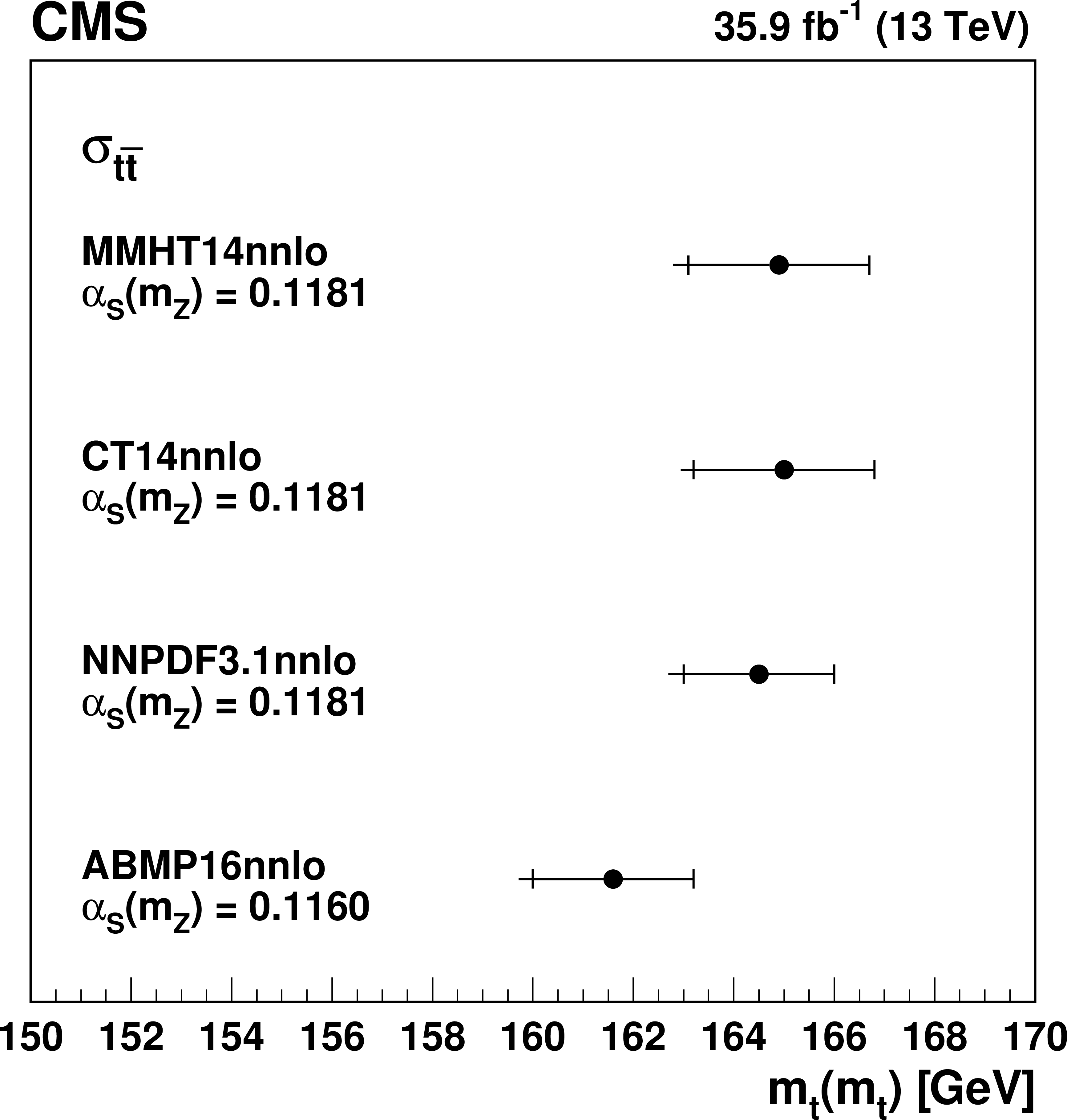
Figure 39:
Values of $ m_{\mathrm{t}}(m_{\mathrm{t}}) $ obtained from comparing the $ \sigma_{{\mathrm{t}\overline{\mathrm{t}}} } $ measurement to the theoretical NNLO predictions using different PDF sets. The inner horizontal bars on the points represent the quadratic sum of the experimental, PDF, and $ \alpha_\mathrm{S}(m_{\mathrm{Z}}) $ uncertainties, while the outer horizontal bars give the total uncertainties. Figure taken from Ref. [63]. |
png pdf |
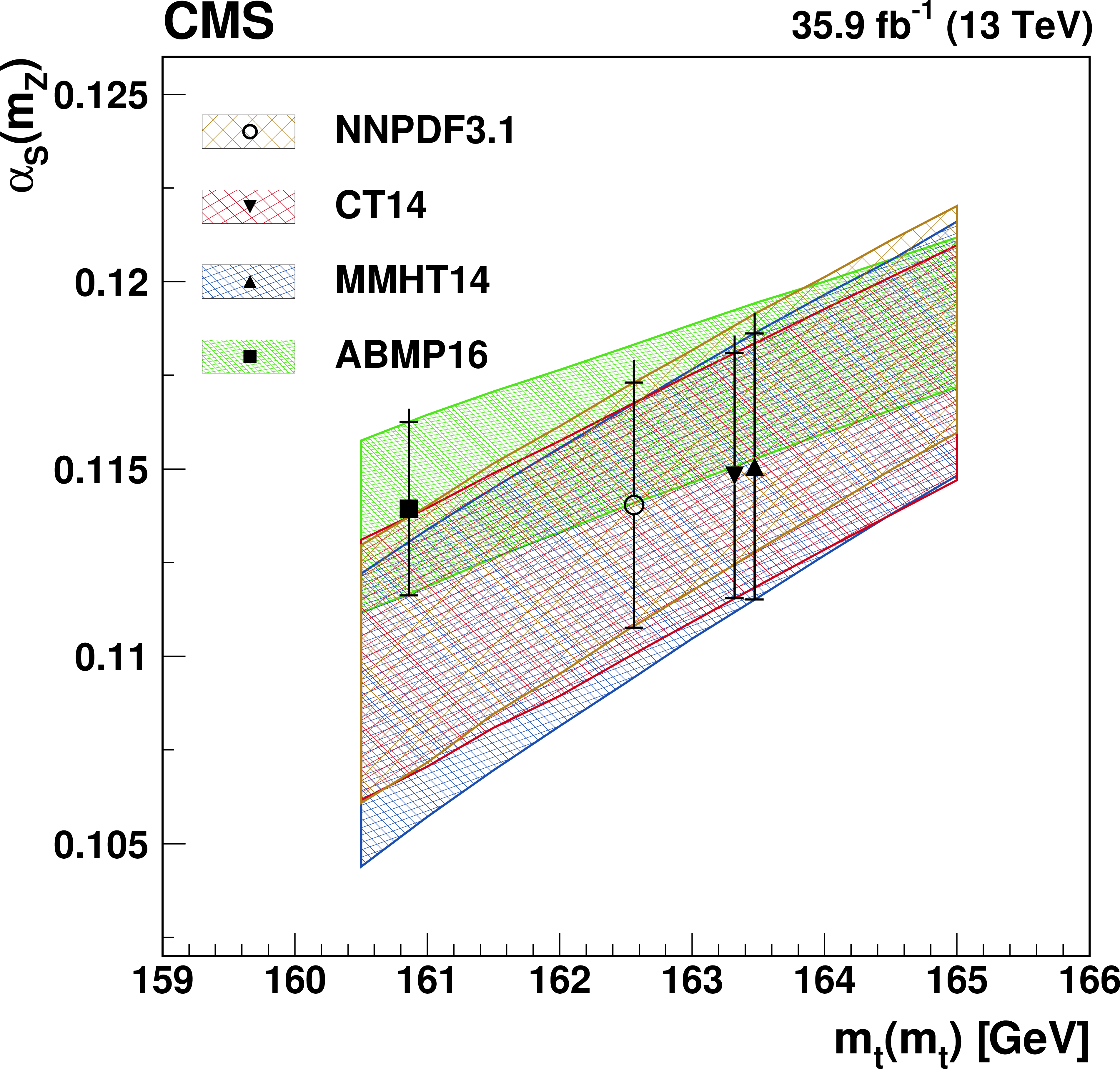
Figure 40:
Values of $ \alpha_\mathrm{S}(m_{\mathrm{Z}}) $ obtained in the comparison of the $ \sigma_{{\mathrm{t}\overline{\mathrm{t}}} } $ measurement to the NNLO prediction using different PDFs, as functions of the $ m_{\mathrm{t}}(m_{\mathrm{t}}) $ value used in the theoretical calculation. The results from using the different PDFs are shown by the bands with different shadings, with the band width corresponding to the quadratic sum of the experimental and PDF uncertainties in $ \alpha_\mathrm{S}(m_{\mathrm{Z}}) $. The resulting measured values of $ \alpha_\mathrm{S}(m_{\mathrm{Z}}) $ are shown by the different style points at the $ m_{\mathrm{t}}(m_{\mathrm{t}}) $ values used for each PDF. The inner vertical bars on the points represent the quadratic sum of the experimental and PDF uncertainties in $ \alpha_\mathrm{S}(m_{\mathrm{Z}}) $, while the outer vertical bars show the total uncertainties. Figure taken from Ref. [63]. |
png pdf |
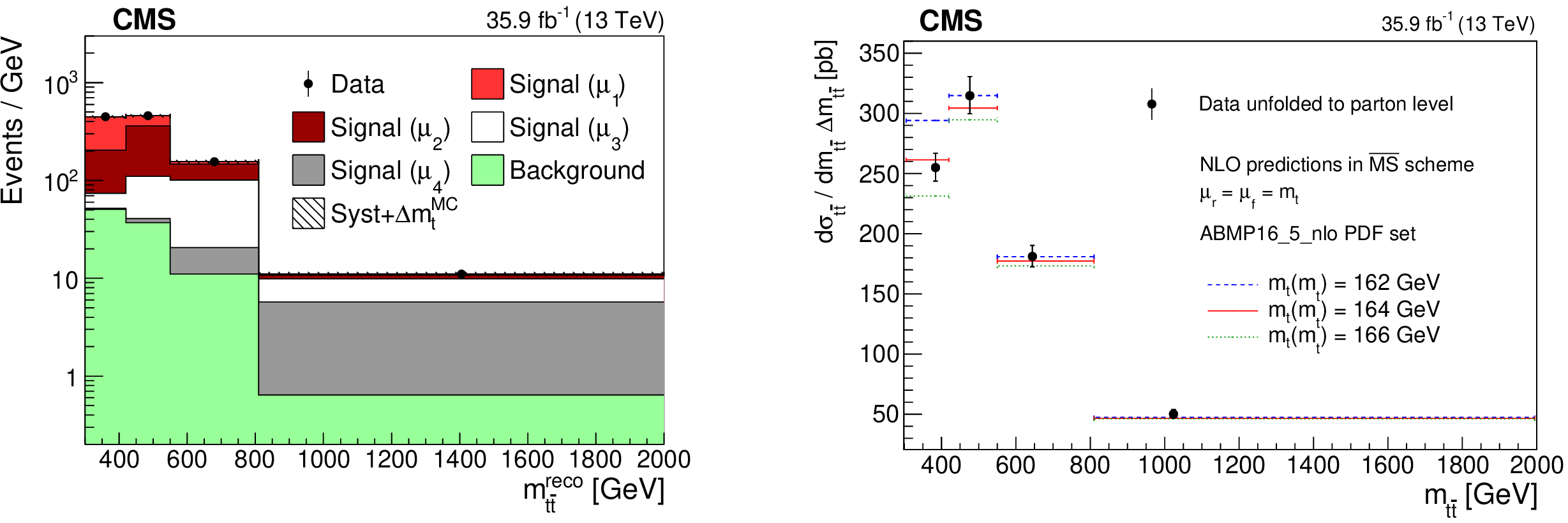
Figure 41:
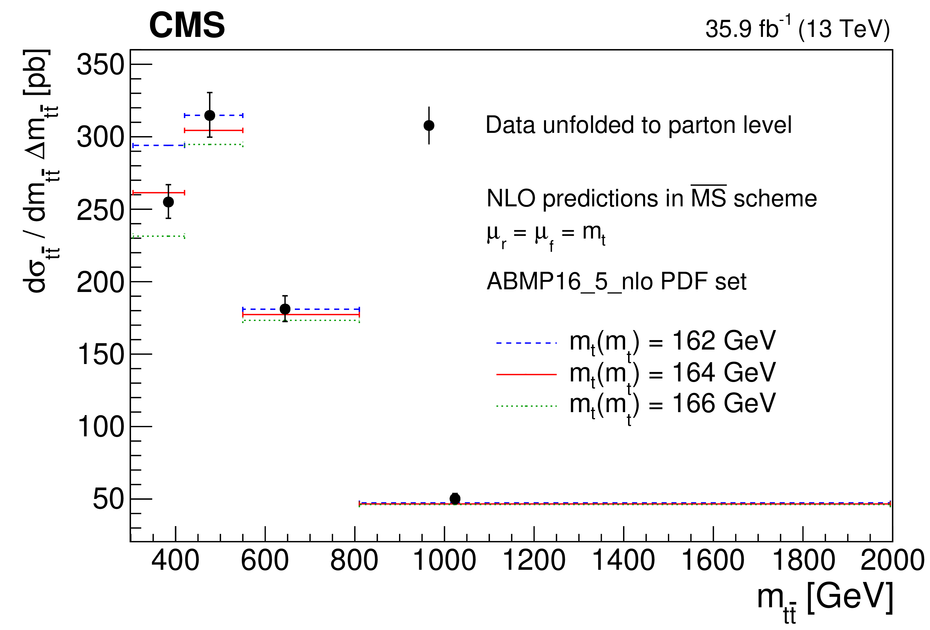
Left: profile likelihood unfolding of the $ m_{{\mathrm{t}\overline{\mathrm{t}}} } $ distribution. The signal sample is split into subprocesses in bins of parton-level $ m_{{\mathrm{t}\overline{\mathrm{t}}} } $, and the signal corresponding to bin $ k $ in $ m_{{\mathrm{t}\overline{\mathrm{t}}} } $ is denoted with ``Signal ($ \mu_{\mathrm{k}} $)''. The vertical bars represent the statistical uncertainty in the data, while the hashed band is the total uncertainty in the MC simulation. Right: unfolded $ \mathrm{t} \overline{\mathrm{t}} $ cross section as a function of $ m_{{\mathrm{t}\overline{\mathrm{t}}} } $, compared to theoretical predictions in the $ \mathrm{\overline{MS}} $ scheme for different values of $ m_{\mathrm{t}}(m_{\mathrm{t}}) $. The vertical bars correspond to the total uncertainty in the unfolded cross section. Here, the bin centres for the unfolded cross section are defined as the average $ m_{{\mathrm{t}\overline{\mathrm{t}}} } $ in the POWHEG+PYTHIA-8 simulation. Figures taken from Ref. [65]. |
png pdf |
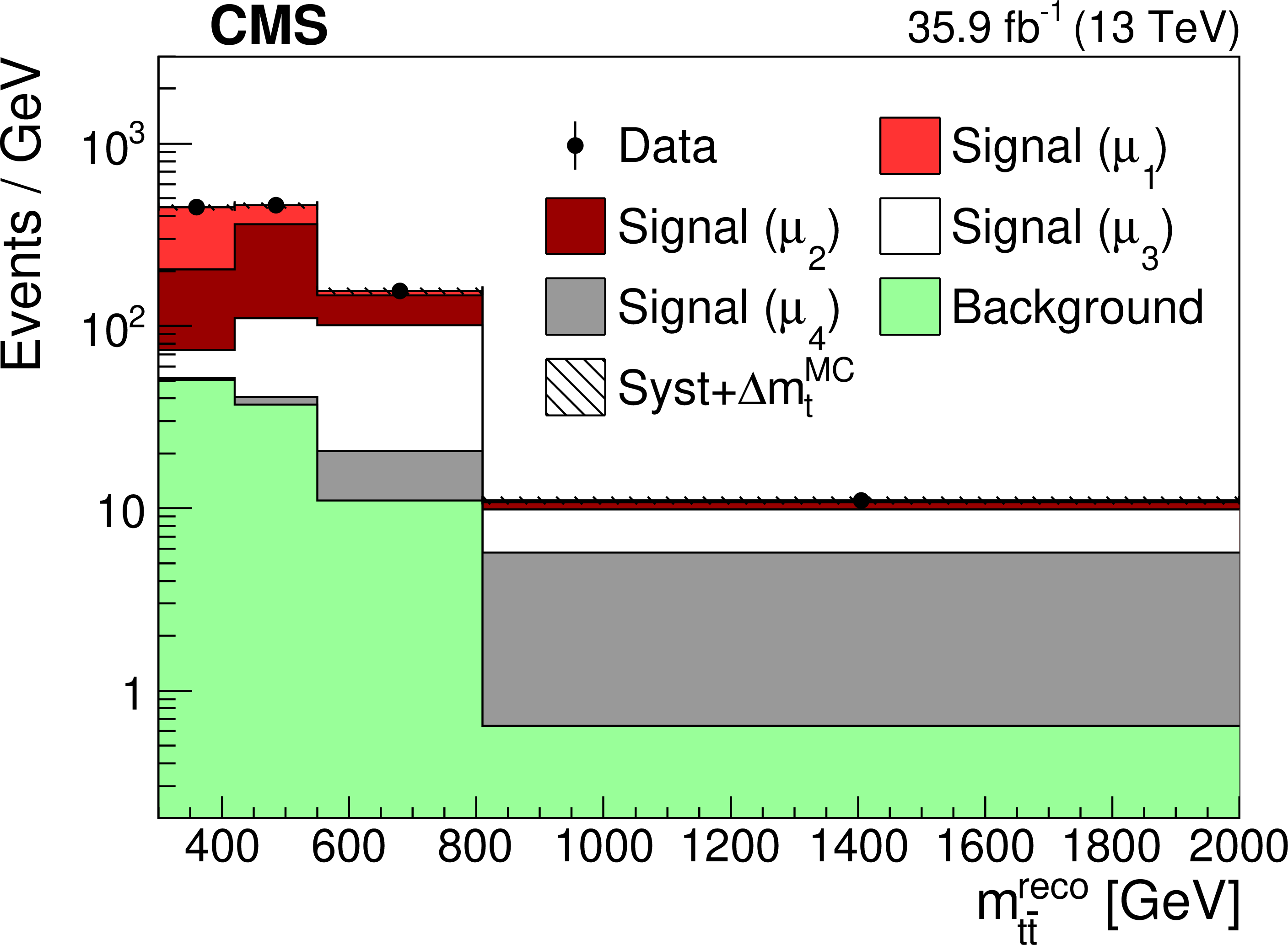
Figure 41-a:
Left: profile likelihood unfolding of the $ m_{{\mathrm{t}\overline{\mathrm{t}}} } $ distribution. The signal sample is split into subprocesses in bins of parton-level $ m_{{\mathrm{t}\overline{\mathrm{t}}} } $, and the signal corresponding to bin $ k $ in $ m_{{\mathrm{t}\overline{\mathrm{t}}} } $ is denoted with ``Signal ($ \mu_{\mathrm{k}} $)''. The vertical bars represent the statistical uncertainty in the data, while the hashed band is the total uncertainty in the MC simulation. Right: unfolded $ \mathrm{t} \overline{\mathrm{t}} $ cross section as a function of $ m_{{\mathrm{t}\overline{\mathrm{t}}} } $, compared to theoretical predictions in the $ \mathrm{\overline{MS}} $ scheme for different values of $ m_{\mathrm{t}}(m_{\mathrm{t}}) $. The vertical bars correspond to the total uncertainty in the unfolded cross section. Here, the bin centres for the unfolded cross section are defined as the average $ m_{{\mathrm{t}\overline{\mathrm{t}}} } $ in the POWHEG+PYTHIA-8 simulation. Figures taken from Ref. [65]. |
png pdf |
Figure 41-b:
Left: profile likelihood unfolding of the $ m_{{\mathrm{t}\overline{\mathrm{t}}} } $ distribution. The signal sample is split into subprocesses in bins of parton-level $ m_{{\mathrm{t}\overline{\mathrm{t}}} } $, and the signal corresponding to bin $ k $ in $ m_{{\mathrm{t}\overline{\mathrm{t}}} } $ is denoted with ``Signal ($ \mu_{\mathrm{k}} $)''. The vertical bars represent the statistical uncertainty in the data, while the hashed band is the total uncertainty in the MC simulation. Right: unfolded $ \mathrm{t} \overline{\mathrm{t}} $ cross section as a function of $ m_{{\mathrm{t}\overline{\mathrm{t}}} } $, compared to theoretical predictions in the $ \mathrm{\overline{MS}} $ scheme for different values of $ m_{\mathrm{t}}(m_{\mathrm{t}}) $. The vertical bars correspond to the total uncertainty in the unfolded cross section. Here, the bin centres for the unfolded cross section are defined as the average $ m_{{\mathrm{t}\overline{\mathrm{t}}} } $ in the POWHEG+PYTHIA-8 simulation. Figures taken from Ref. [65]. |
png pdf |
Figure 42:
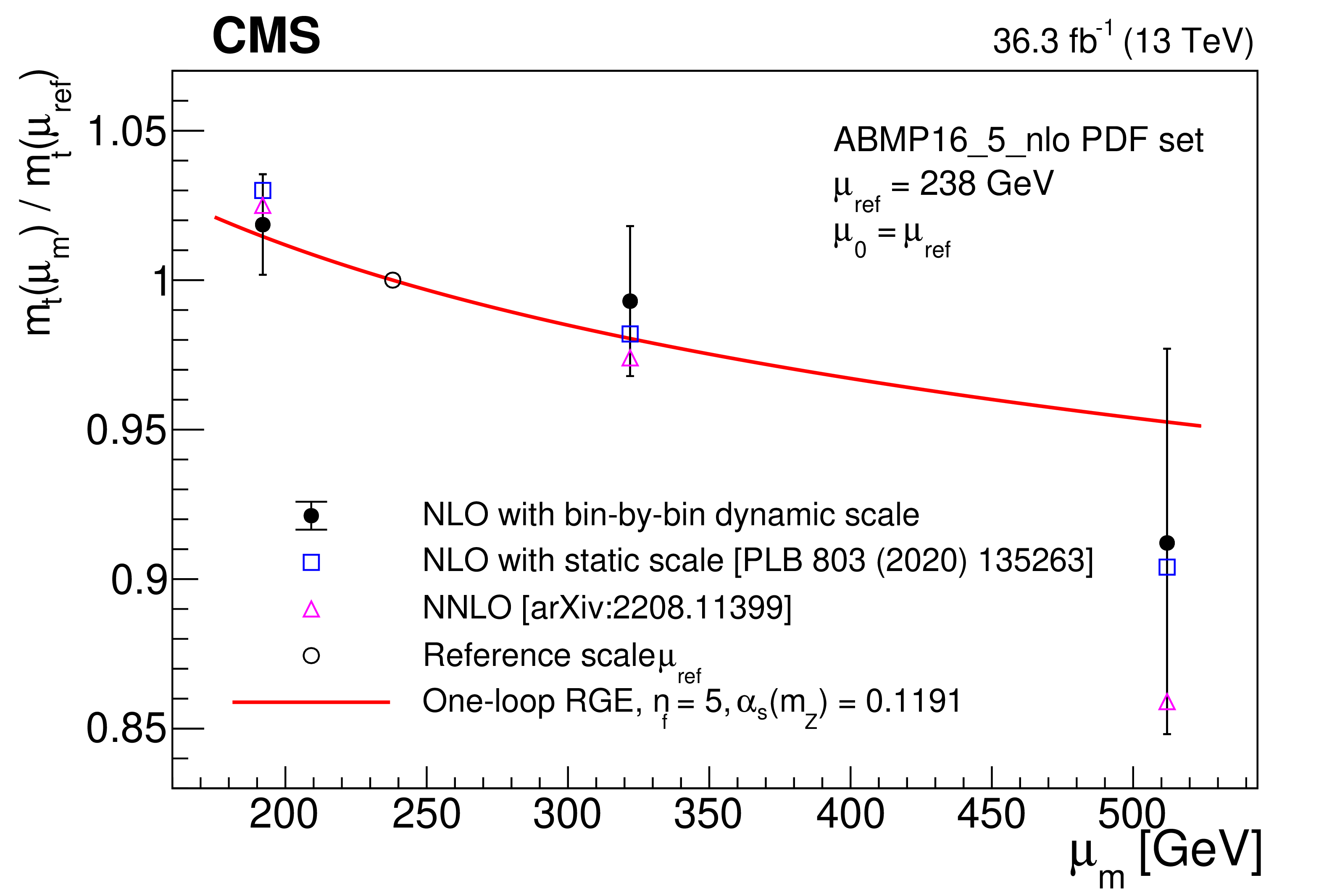
Running of the top quark mass as a function of $ \mu_{\mathrm{m}}=m_{{\mathrm{t}\overline{\mathrm{t}}} }/ $ 2 obtained with a bin-by-bin dynamic scale $ \mu_{\mathrm{k}}/ $ 2 (full circles), compared to the central values of the results of Ref. [65] obtained with a constant scale $ \mu_{\mathrm{m}}=\mu_{\mathrm{k}} $ (hollow squares) and to those of the NNLO results of Ref. [241] (hollow triangles). As in Ref. [65], the error bars indicate the combination of experimental, extrapolation, and PDF uncertainties in the NLO extraction with bin-by-bin dynamic scale. The full treatment of the QCD scale variations can be found in Ref. [241]. The assumptions on the renormalisation and factorisation scales adopted in the different interpretations are summarised in Table 6. The uncertainties in the three results, which are mostly correlated, are given in the respective references and are of comparable size. |

png pdf |
Figure 43:
The fractional uncertainties in the gluon distribution function of the proton as a function of $ x $ at factorisation scale $ \mu_{\mathrm{f}}^2= $ 10$^5$ GeV$^{2}$ from a QCD analysis using the DIS and CMS muon charge asymmetry measurements (hatched area), and also including the CMS $ \sigma_{{\mathrm{t}\overline{\mathrm{t}}} } $ results at $ \sqrt{s} = $ 5.02 TeV (solid area). The relative uncertainties are found after the two gluon distributions have been normalised to unity. The solid line shows the ratio of the gluon distribution function found from the fit with the CMS $ \sigma_{{\mathrm{t}\overline{\mathrm{t}}} } $ measurements included to that found without. Figure taken from Ref. [242]. |
png pdf |
Figure 44:
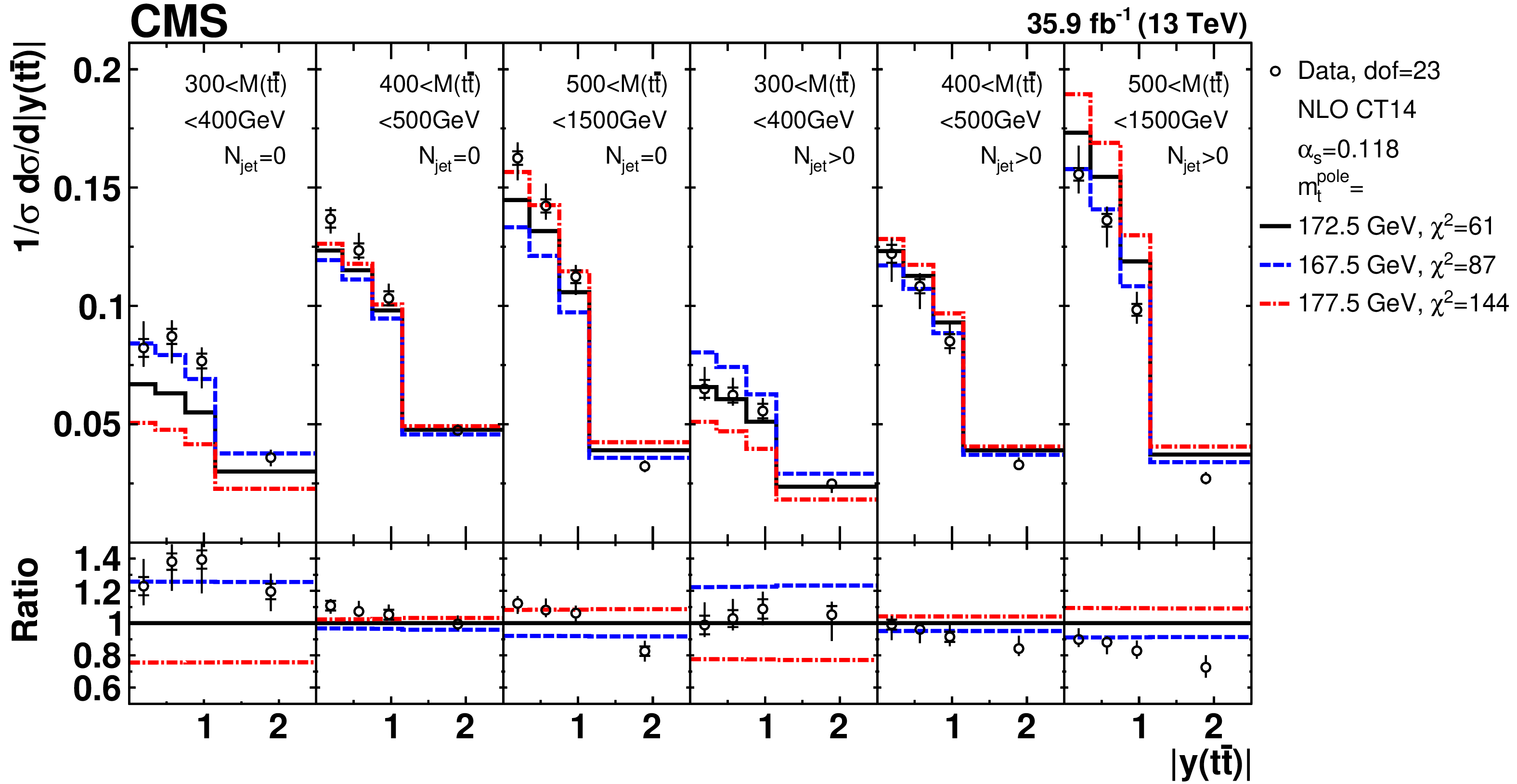
Comparison of the measured $ [N_{\text{jet}}^{0,1+},m_{{\mathrm{t}\overline{\mathrm{t}}} },y_{{\mathrm{t}\overline{\mathrm{t}}} }] $ cross sections to NLO predictions obtained using different $ m_{\mathrm{t}}^{\text{pole}} $ values. For each theoretical prediction, values of $ \chi^2 $ and dof for the comparison to the data are reported. Figure taken from Ref. [64]. |
png pdf |
Figure 45:
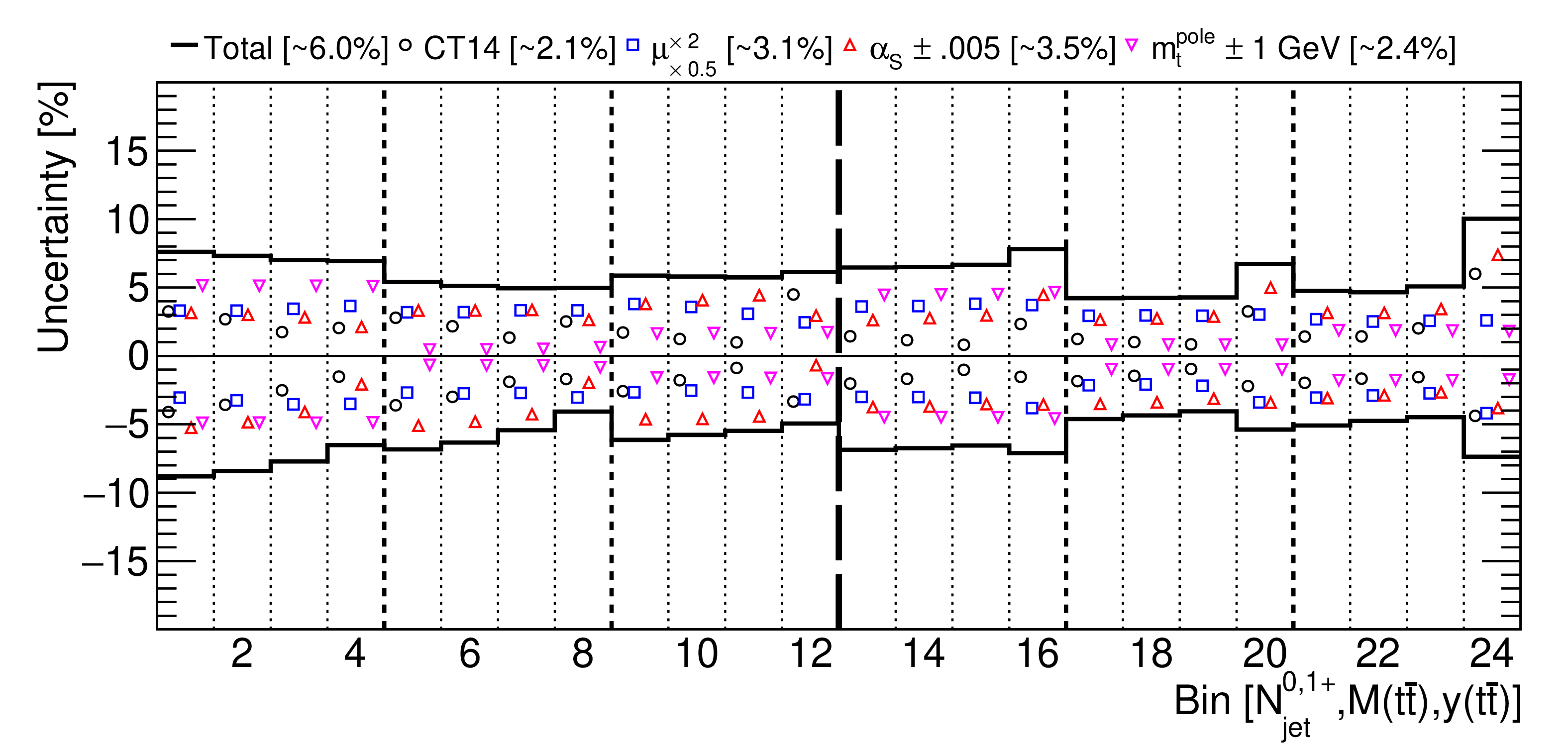
The theoretical uncertainties for $ [N_{\text{jet}}^{0,1+},m_{{\mathrm{t}\overline{\mathrm{t}}} },y_{{\mathrm{t}\overline{\mathrm{t}}} }] $ cross sections, arising from the scale, PDF, $ \alpha_\mathrm{S}(m_{\mathrm{Z}}) $, and $ m_{\mathrm{t}} $ variations, as well as the total theoretical uncertainties obtained from variations in $ \mu_{\mathrm{r}} $ and $ \mu_{\mathrm{f}} $, with their bin-averaged values shown in brackets. The bins are the same as in Fig. 44. Figure taken from Ref. [64]. |
png pdf |
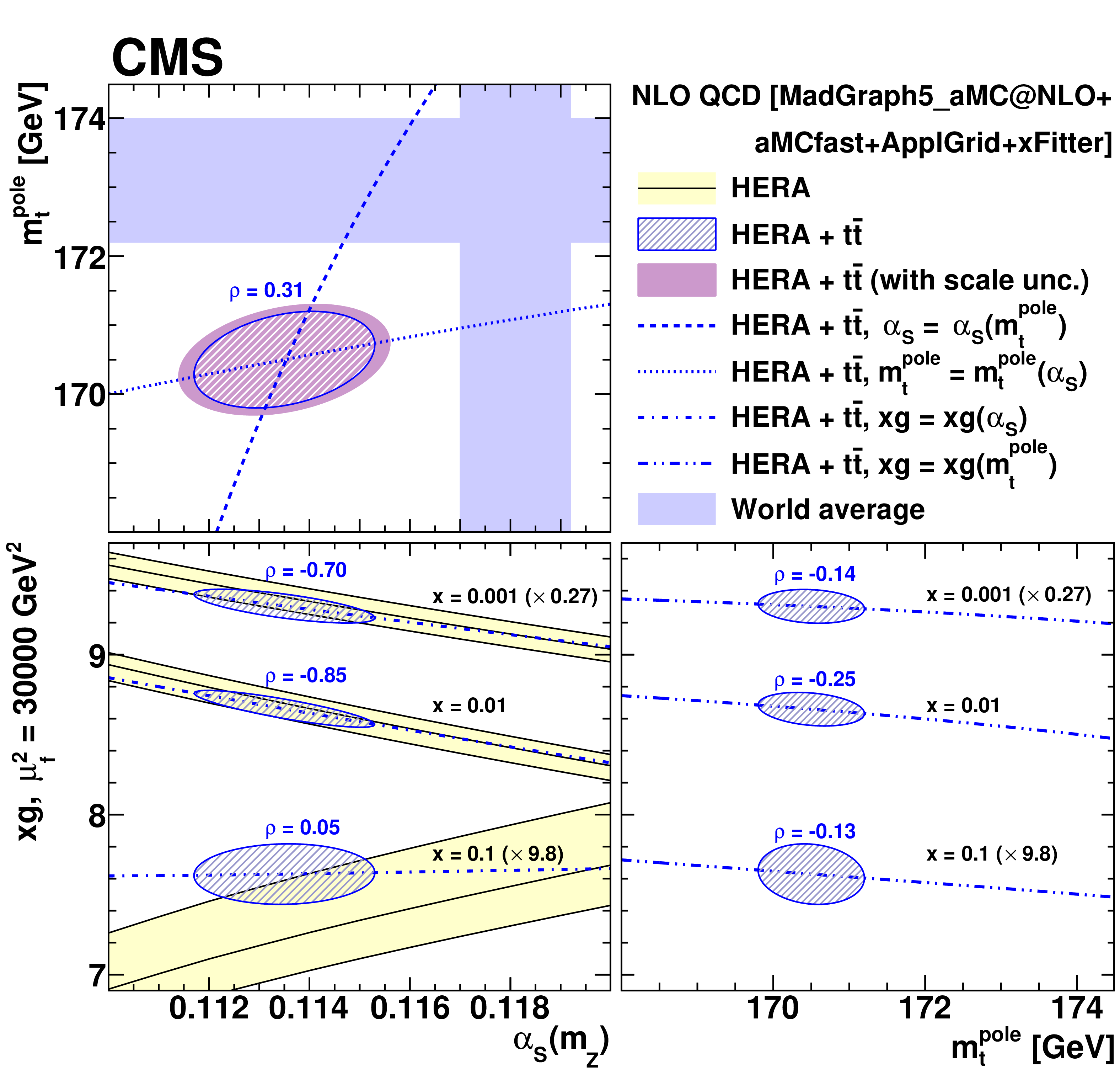
Figure 46:
The extracted values and their correlations for $ \alpha_\mathrm{S} $ and $ m_{\mathrm{t}}^{\text{pole}} $ (upper left), $ \alpha_\mathrm{S} $ and gluon PDF (lower left), and $ m_{\mathrm{t}}^{\text{pole}} $ and gluon PDF (lower, right). The gluon PDF is shown at the scale $ \mu_{\mathrm{f}}^2= $ 30 000 GeV$^{2}$ for several values of $ x $. For the extracted values of $ \alpha_\mathrm{S} $ and $ m_{\mathrm{t}}^{\text{pole}} $, the additional uncertainties arising from the dependence on the scale are shown. The correlation coefficients $ \rho $ as defined in Ref. [64] are displayed. Furthermore, values of $ \alpha_\mathrm{S} $ ($ m_{\mathrm{t}}^{\text{pole}} $, gluon PDF) extracted using fixed values of $ m_{\mathrm{t}}^{\text{pole}}(\alpha_\mathrm{S}) $ are displayed as dashed, dotted, or dash-dotted lines. The world average values $ \alpha_\mathrm{S}(m_{\mathrm{Z}})= $ 0.1181 $ \pm $ 0.0011 and $ m_{\mathrm{t}}^{\text{pole}}= $ 173.1 $ \pm $ 0.9 GeV from Ref. [252] are shown for reference. Figure taken from Ref. [64]. |
png pdf |
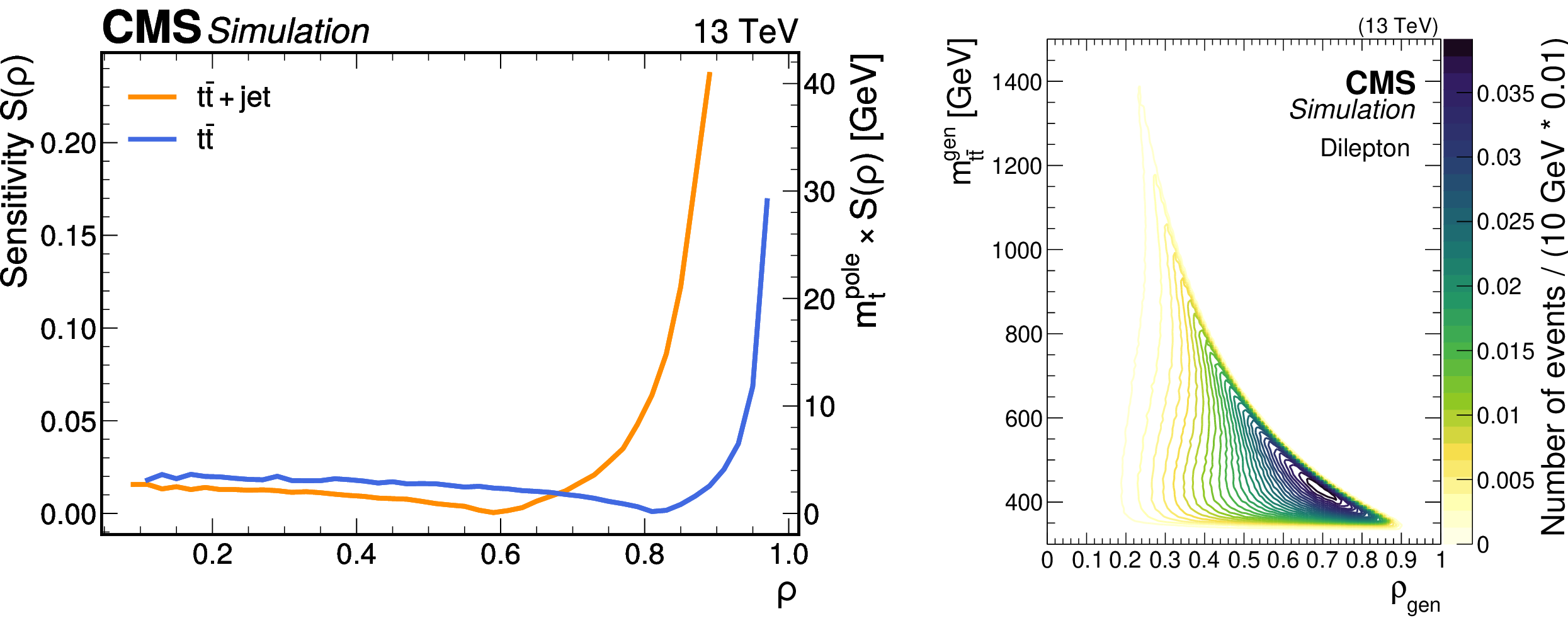
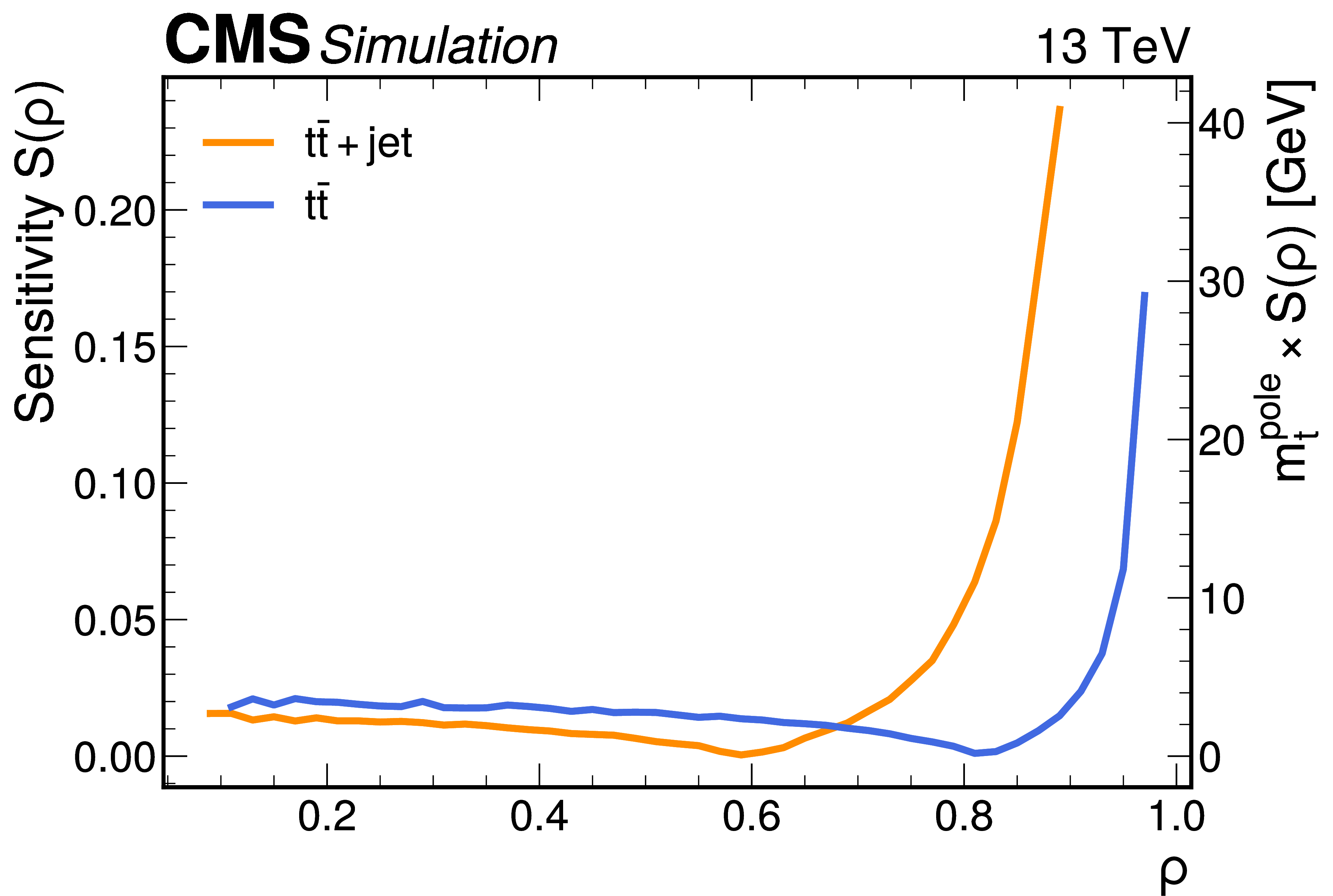
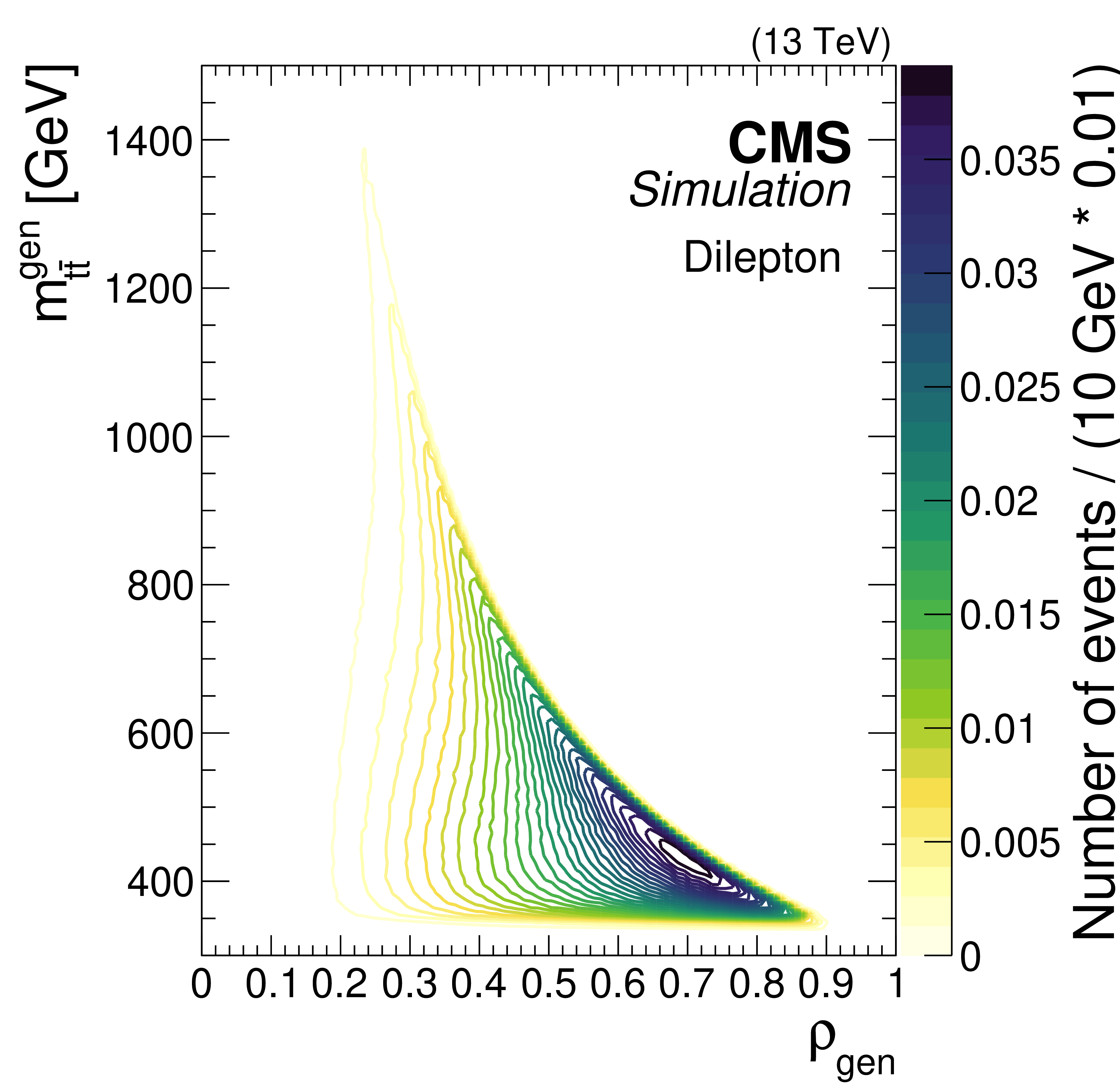
Figure 47:
Left: Sensitivity $ \mathcal{S} $ to the value of $ m_{\mathrm{t}}^{\text{pole}} $ for $ \mathrm{t} \overline{\mathrm{t}} $ (blue) and $ {\mathrm{t}\overline{\mathrm{t}}} \text{+jet} $ production (orange). Figure taken from Ref. [69]. Right: The distribution of $ m_{{\mathrm{t}\overline{\mathrm{t}}} } $ at the parton level as given by the POWHEG+PYTHIA-8 $ \mathrm{t} \overline{\mathrm{t}} $ simulation as a function of $ \rho $ at parton level, obtained in Ref. [69]. |
png pdf |
Figure 47-a:
Left: Sensitivity $ \mathcal{S} $ to the value of $ m_{\mathrm{t}}^{\text{pole}} $ for $ \mathrm{t} \overline{\mathrm{t}} $ (blue) and $ {\mathrm{t}\overline{\mathrm{t}}} \text{+jet} $ production (orange). Figure taken from Ref. [69]. Right: The distribution of $ m_{{\mathrm{t}\overline{\mathrm{t}}} } $ at the parton level as given by the POWHEG+PYTHIA-8 $ \mathrm{t} \overline{\mathrm{t}} $ simulation as a function of $ \rho $ at parton level, obtained in Ref. [69]. |
png pdf |
Figure 47-b:
Left: Sensitivity $ \mathcal{S} $ to the value of $ m_{\mathrm{t}}^{\text{pole}} $ for $ \mathrm{t} \overline{\mathrm{t}} $ (blue) and $ {\mathrm{t}\overline{\mathrm{t}}} \text{+jet} $ production (orange). Figure taken from Ref. [69]. Right: The distribution of $ m_{{\mathrm{t}\overline{\mathrm{t}}} } $ at the parton level as given by the POWHEG+PYTHIA-8 $ \mathrm{t} \overline{\mathrm{t}} $ simulation as a function of $ \rho $ at parton level, obtained in Ref. [69]. |

png pdf |
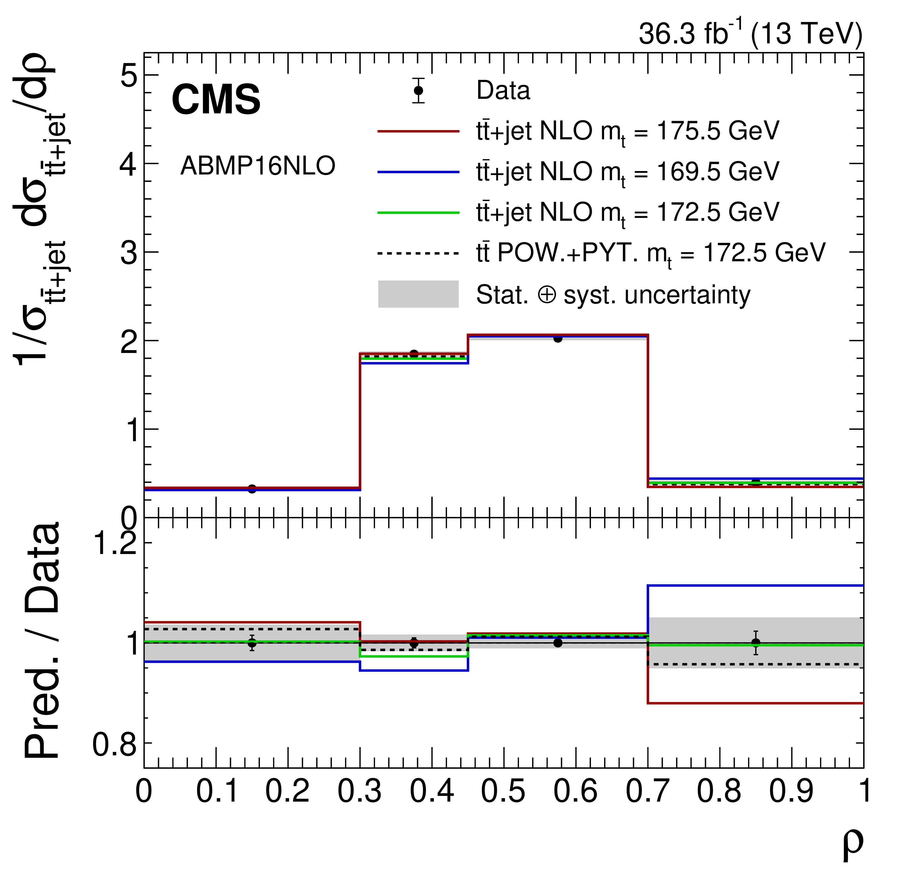
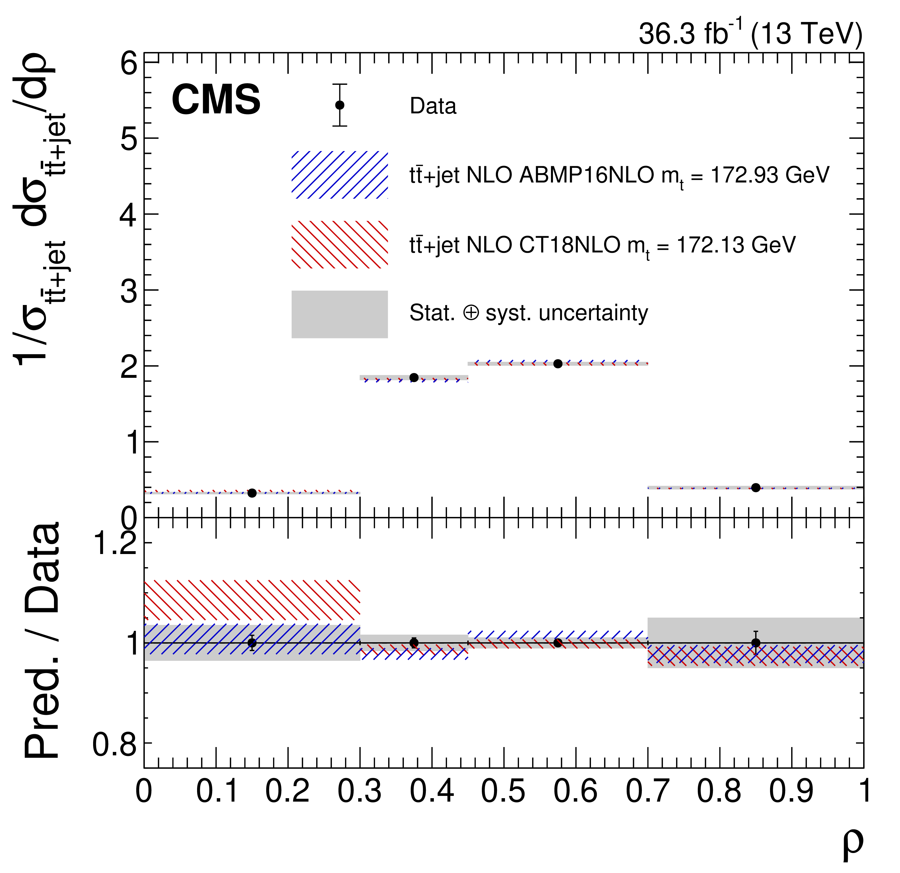
Figure 48:
The measured normalised $ {\mathrm{t}\overline{\mathrm{t}}} \text{+jet} $ differential cross section (closed symbols) as a function of $ \rho $. The vertical error bars (shaded areas) show the statistical (statistical plus systematic) uncertainty. The data are compared to theoretical predictions and the POWHEG+PYTHIA-8 simulation, either using alternative values of $ m_{\mathrm{t}} $ (left panel), shown by the solid lines, or two alternative PDF sets (right), shown by the hatched areas. In the lower panels, the ratio of the predictions to the measurement is shown. Figures taken from Ref. [69]. |
png pdf |
Figure 48-a:
The measured normalised $ {\mathrm{t}\overline{\mathrm{t}}} \text{+jet} $ differential cross section (closed symbols) as a function of $ \rho $. The vertical error bars (shaded areas) show the statistical (statistical plus systematic) uncertainty. The data are compared to theoretical predictions and the POWHEG+PYTHIA-8 simulation, either using alternative values of $ m_{\mathrm{t}} $ (left panel), shown by the solid lines, or two alternative PDF sets (right), shown by the hatched areas. In the lower panels, the ratio of the predictions to the measurement is shown. Figures taken from Ref. [69]. |
png pdf |
Figure 48-b:
The measured normalised $ {\mathrm{t}\overline{\mathrm{t}}} \text{+jet} $ differential cross section (closed symbols) as a function of $ \rho $. The vertical error bars (shaded areas) show the statistical (statistical plus systematic) uncertainty. The data are compared to theoretical predictions and the POWHEG+PYTHIA-8 simulation, either using alternative values of $ m_{\mathrm{t}} $ (left panel), shown by the solid lines, or two alternative PDF sets (right), shown by the hatched areas. In the lower panels, the ratio of the predictions to the measurement is shown. Figures taken from Ref. [69]. |
png pdf |
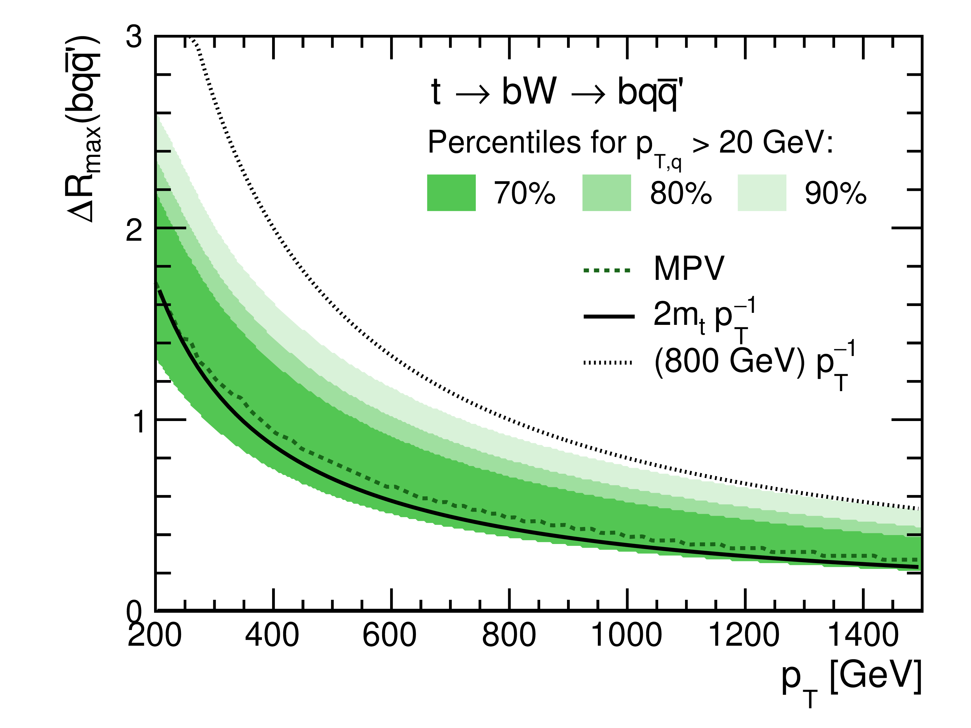
Figure 49:
Percentiles of maximum angular distance between the top quark decay partons as a function of the top quark $ p_{\mathrm{T}} $ obtained from $ \mathrm{t} \overline{\mathrm{t}} $ simulation. The filled bands indicate the areas that are populated by 70, 80, and 90% of all simulated $ \mathrm{t} \overline{\mathrm{t}} $ events, where the decay partons have at least $ p_{\mathrm{T}} > $ 20 GeV. The most probable value (MPV) is shown as a dashed line, and two functional forms are shown that approximate the $ p_{\mathrm{T}} $-dependence of $ \Delta R_{\text{max}} $. Figure taken from Ref. [271]. |
png pdf |
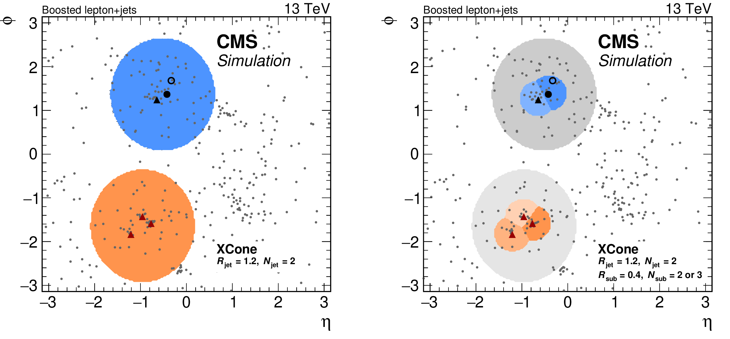
Figure 50:
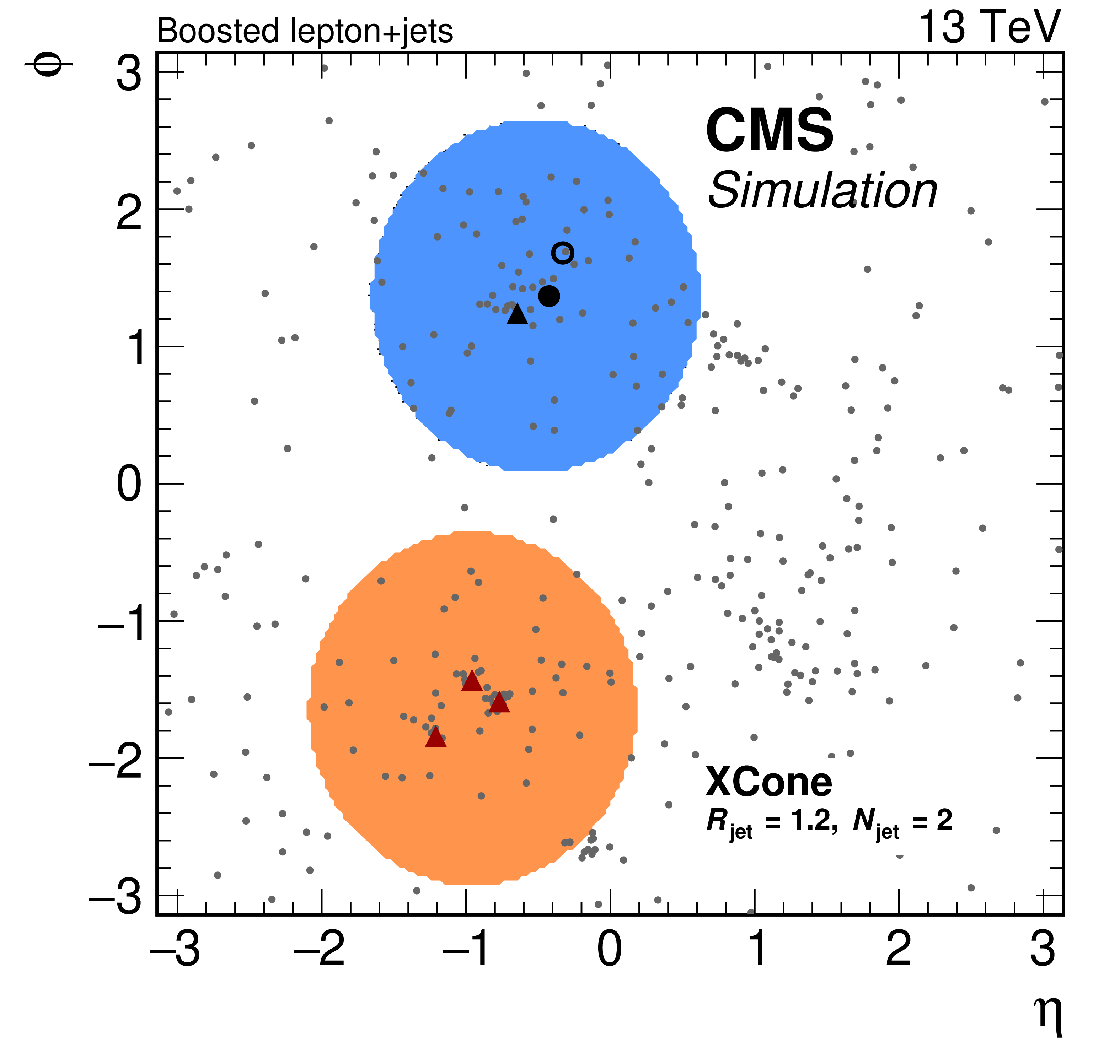
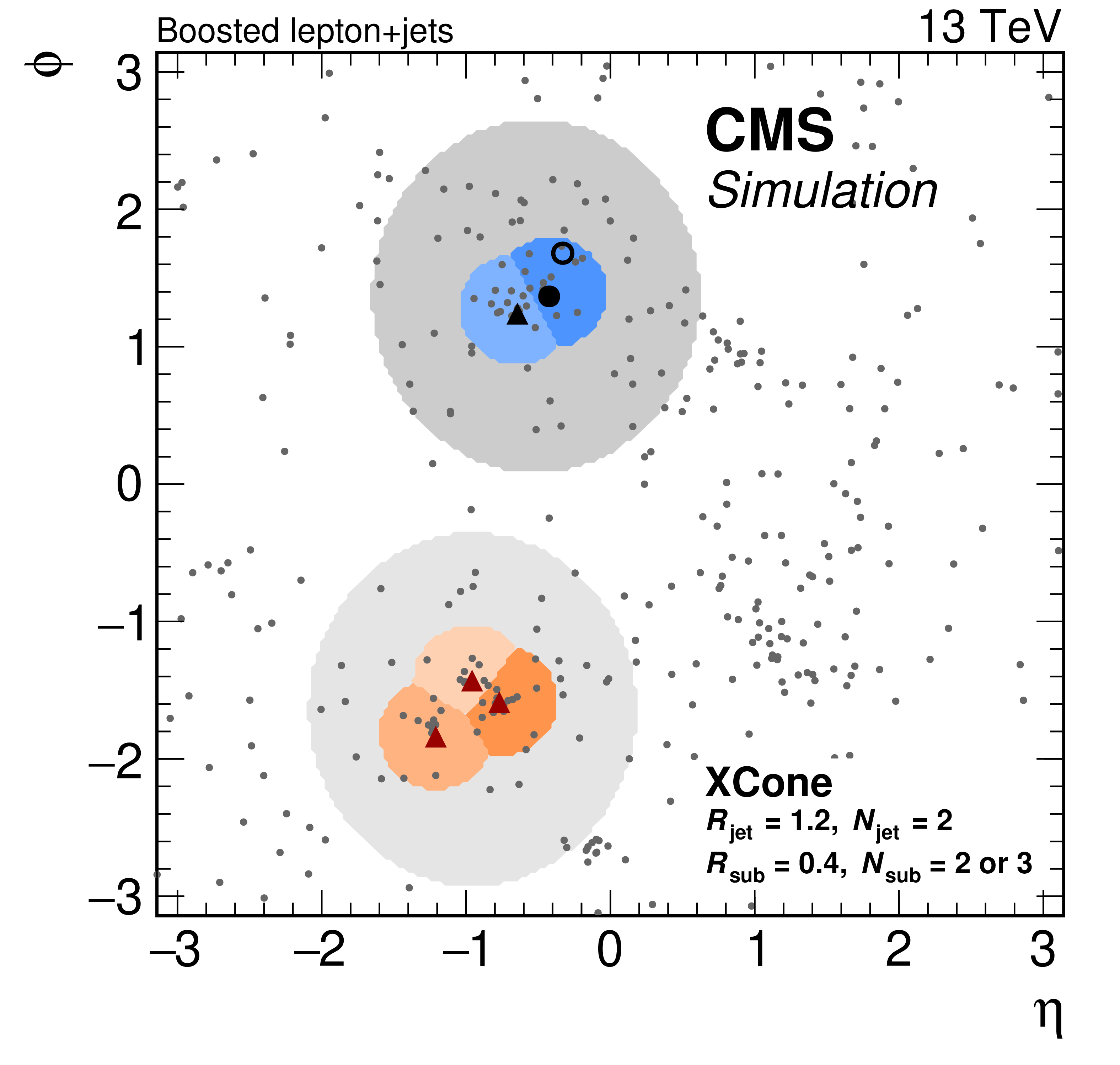
Display of a simulated $ \mathrm{t} \overline{\mathrm{t}} $ event. Each point marks the position of a particle at the particle level in the $ \eta\text{-}\phi $ plane. Decay products of the top quarks are highlighted with triangles or larger circles. The red triangles mark the three quarks from the hadronic decay; the black triangle, black circle, and open circle correspond to the b quark, charged lepton, and neutrino from the leptonic top quark decay, respectively. The jet areas are shown as coloured shapes. The left panel shows the first clustering step with $ N= $ 2 and $ R= $ 1.2, while the right panel shows the subjet clustering. |
png pdf |
Figure 50-a:
Display of a simulated $ \mathrm{t} \overline{\mathrm{t}} $ event. Each point marks the position of a particle at the particle level in the $ \eta\text{-}\phi $ plane. Decay products of the top quarks are highlighted with triangles or larger circles. The red triangles mark the three quarks from the hadronic decay; the black triangle, black circle, and open circle correspond to the b quark, charged lepton, and neutrino from the leptonic top quark decay, respectively. The jet areas are shown as coloured shapes. The left panel shows the first clustering step with $ N= $ 2 and $ R= $ 1.2, while the right panel shows the subjet clustering. |
png pdf |
Figure 50-b:
Display of a simulated $ \mathrm{t} \overline{\mathrm{t}} $ event. Each point marks the position of a particle at the particle level in the $ \eta\text{-}\phi $ plane. Decay products of the top quarks are highlighted with triangles or larger circles. The red triangles mark the three quarks from the hadronic decay; the black triangle, black circle, and open circle correspond to the b quark, charged lepton, and neutrino from the leptonic top quark decay, respectively. The jet areas are shown as coloured shapes. The left panel shows the first clustering step with $ N= $ 2 and $ R= $ 1.2, while the right panel shows the subjet clustering. |
png pdf |
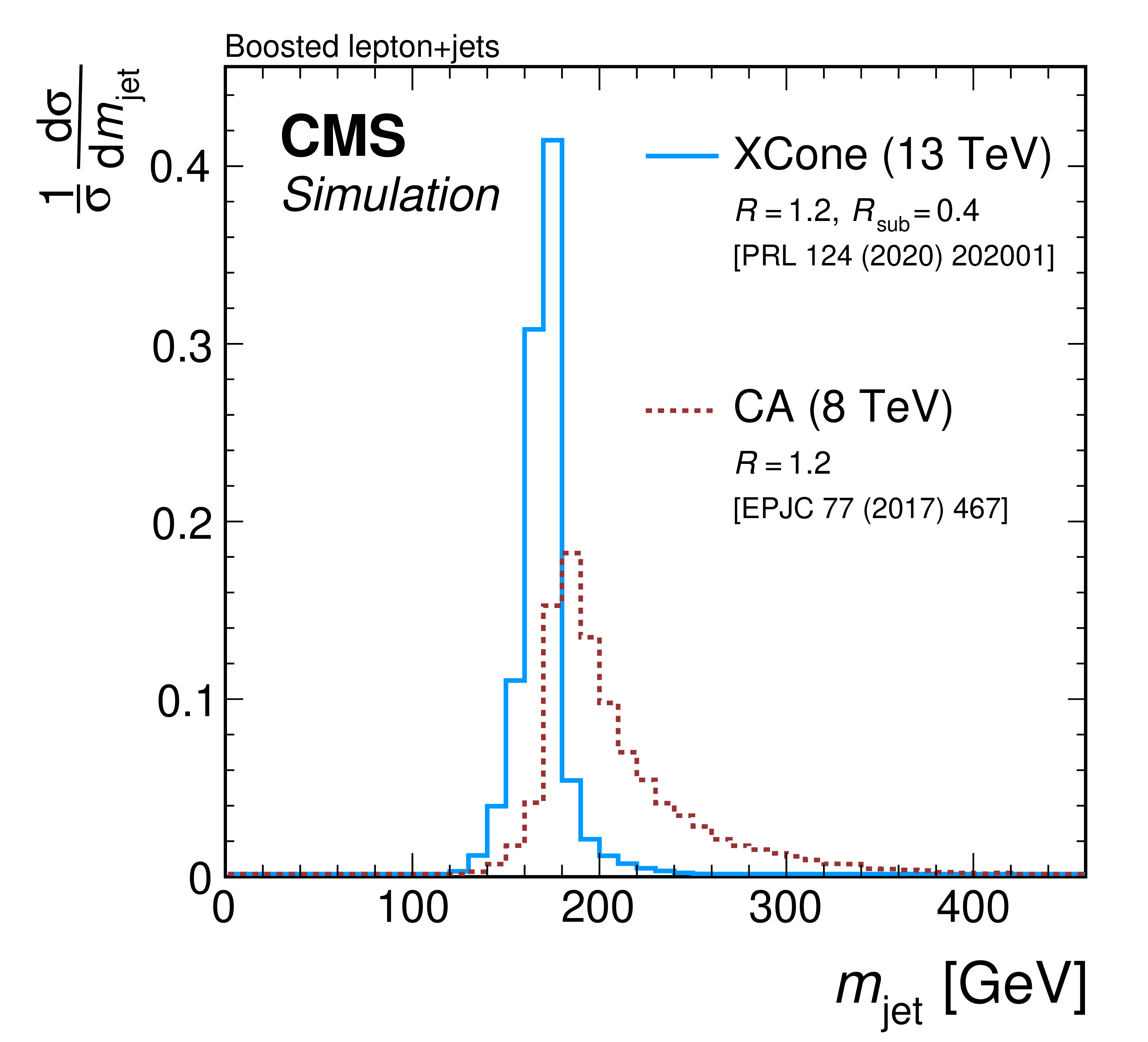
Figure 51:
Normalised jet mass distribution at the particle level for the two-step XCone clustering (blue solid) used in Ref. [66,70] and CA jets with $ R= $ 1.2 (red dotted) used in Ref. [59]. Only events where all top quark decay products are within $ \Delta R= $ 0.4 to any XCone subjet or within $ \Delta R= $ 1.2 to the CA jet are shown. |
png pdf |
Figure 52:
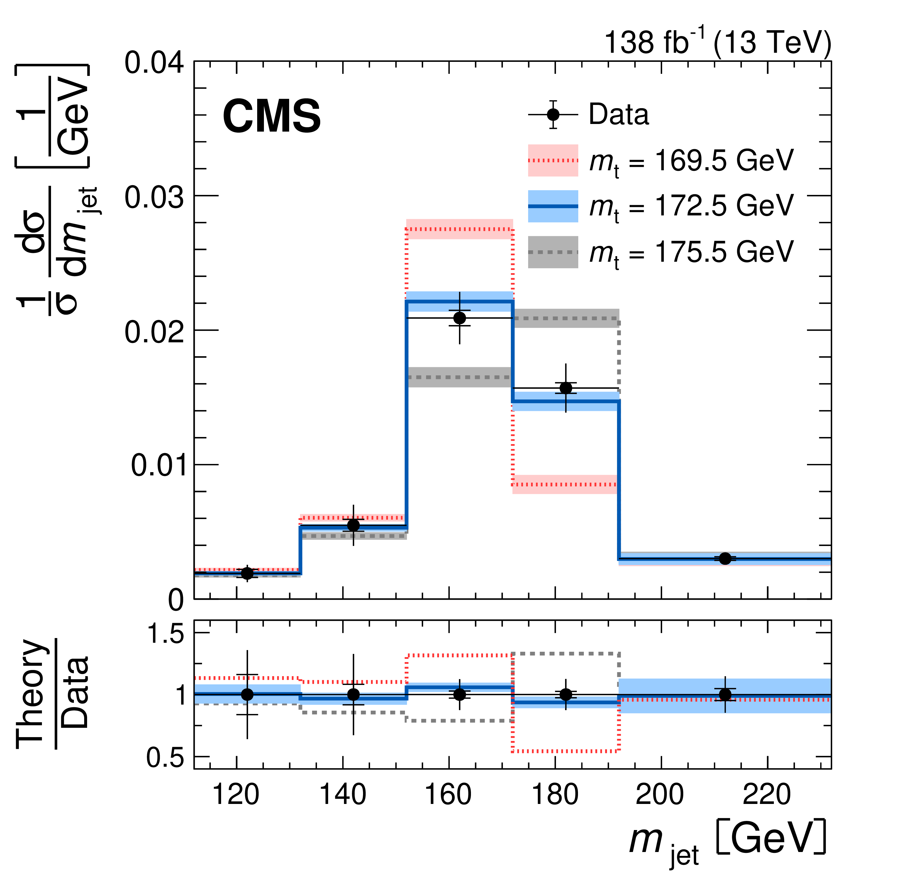
Normalised differential $ \mathrm{t} \overline{\mathrm{t}} $ production cross section as a function of $ m_{\text{jet}} $. Data (markers) are compared to predictions for different $ m_{\mathrm{t}} $ obtained from simulation (lines). The bars on the markers display the statistical (inner bars) and total (outer bars) uncertainties. The theoretical uncertainty is shown as coloured area. Figure taken from Ref. [70]. |
png pdf |
Figure 53:
Summary of the $ m_{\mathrm{t}} $ extraction in $ m_{\text{jet}} $ measurements. The left panel shows the extracted value of $ m_{\mathrm{t}} $ (marker) with statistical (thick bars) and total (thin bars) uncertainties. The right panel displays a breakdown of contributing uncertainty groups and their impact on the uncertainty in the $ m_{\mathrm{t}} $ extraction. The figure is compiled from Refs. [59,66,70]. |
png pdf |
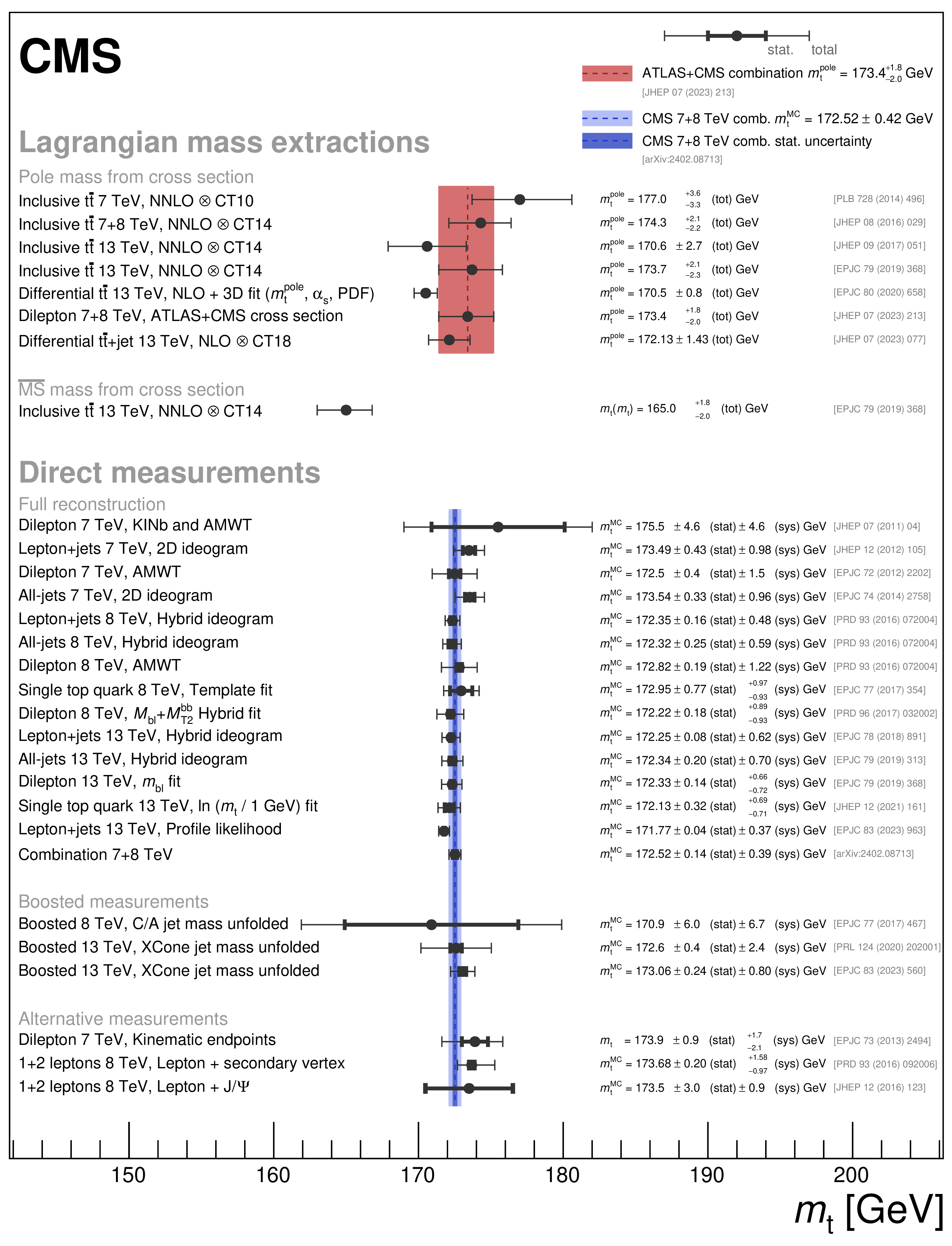
Figure 54:
Overview of top quark mass measurement results published by the CMS Collaboration. The markers display the respective measured value of $ m_{\mathrm{t}} $ with the statistical (inner) and total (outer) uncertainties shown as horizontal error bars. The measurements are categorised into Lagrangian mass extractions from cross section measurements and direct measurements of $ m_{\mathrm{t}}^{\text{MC}} $ and are compared to the combined cross section measurement of the ATLAS and CMS Collaborations (red) and a CMS combination of Run-1 results (blue). Similar labelling as in Table 1 is used. The figure is compiled from Refs. [47,48,49,50,51,52,53,54,55,56,57,58,59,60,61,62,63,64,66,67,68,69,70,71,72]. |

png pdf |
Figure 55:
The resolution of the $ \mu+\mathrm{J}/\psi $ mass for the CMS Phase-2 upgraded detector, for the two PU scenarios, and for the Run-2 (Phase-0) detector. Figure taken from Ref. [290]. |
png pdf |
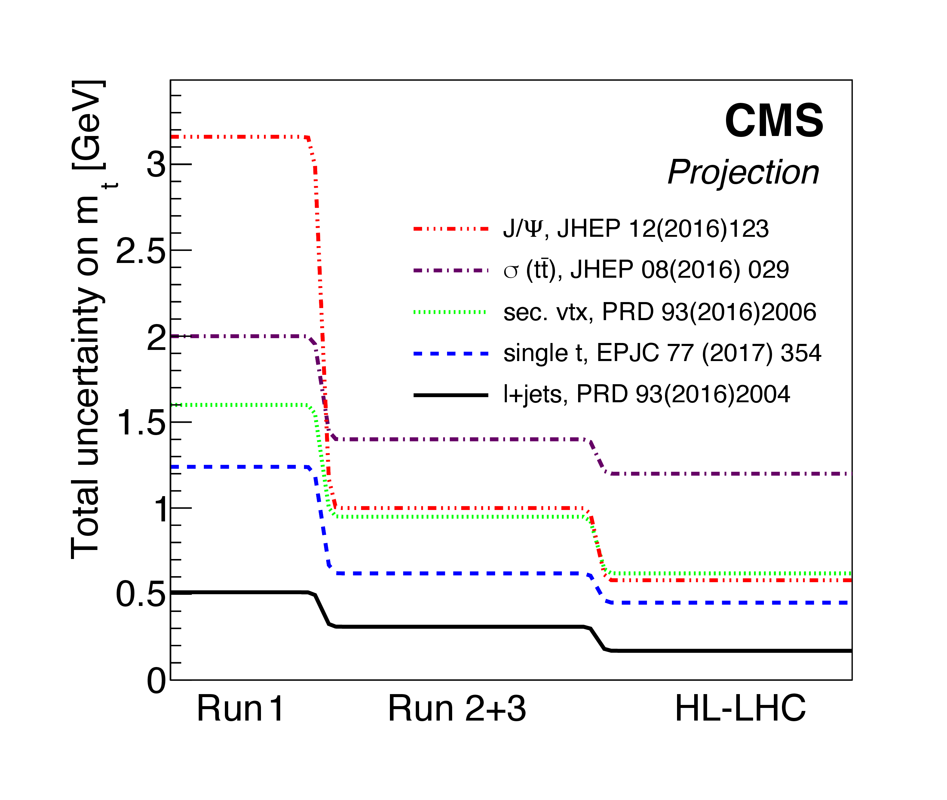
Figure 56:
Total uncertainty in $ m_{\mathrm{t}} $ obtained with a selection of different measurement methods and their projections for expected running conditions in Run-2 + Run-3 and at the HL-LHC. The projections are based on $ m_{\mathrm{t}} $ measurements performed during the LHC Run-1, also listed in Table 1: the $ \mathrm{J}/\psi $ [56], total $ \mathrm{t} \overline{\mathrm{t}} $ cross section [54] in the dilepton channel, secondary vertex [55], single top quark [58], and lepton+jets direct [53] measurements. These projections do not fully account for improvements in the performance of the upgraded CMS detector. Figure taken from Ref. [294]. |

png pdf |
Figure 57:
Left: The projected total experimental uncertainty in the top quark pair production cross section as a function of the uncertainty in the integrated luminosity, for two experimental scenarios, assuming no reduction of the experimental uncertainties with respect to Run-2 and a reduction of the uncertainties following the recommendations outlined in Ref [295]. Right: The projected relative uncertainties in the extracted values of $ m_{\mathrm{t}} $ (dotted lines) and $ \alpha_\mathrm{S} $ (solid lines) as a function of the uncertainty in the integrated luminosity, comparing the case of the full uncertainty in the prediction and no uncertainty in the prediction. The results are obtained assuming a reduction of the uncertainties in the measurement to 1.5%. Figure taken from Ref. [296]. |

png pdf |
Figure 57-a:
Left: The projected total experimental uncertainty in the top quark pair production cross section as a function of the uncertainty in the integrated luminosity, for two experimental scenarios, assuming no reduction of the experimental uncertainties with respect to Run-2 and a reduction of the uncertainties following the recommendations outlined in Ref [295]. Right: The projected relative uncertainties in the extracted values of $ m_{\mathrm{t}} $ (dotted lines) and $ \alpha_\mathrm{S} $ (solid lines) as a function of the uncertainty in the integrated luminosity, comparing the case of the full uncertainty in the prediction and no uncertainty in the prediction. The results are obtained assuming a reduction of the uncertainties in the measurement to 1.5%. Figure taken from Ref. [296]. |
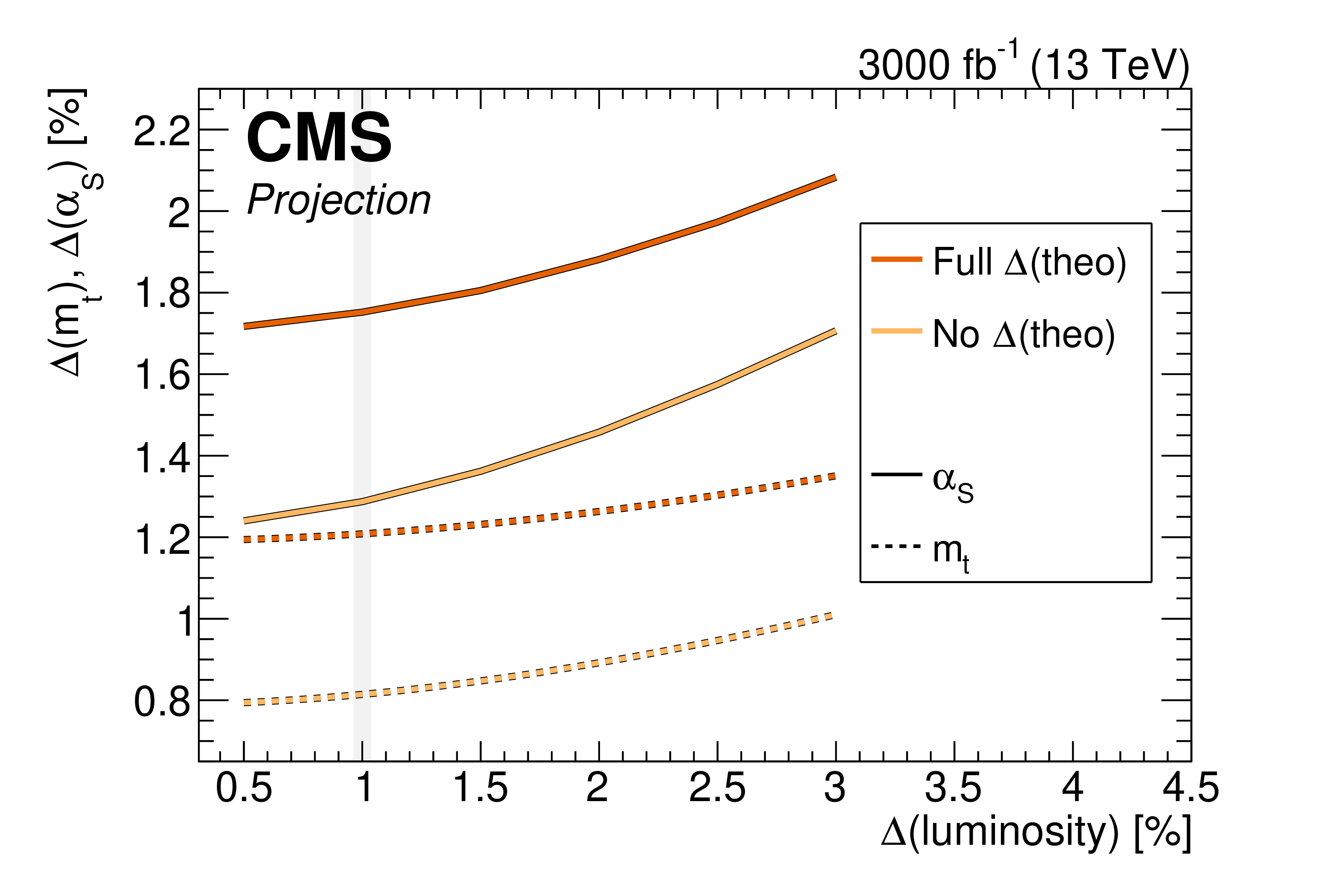
png pdf |
Figure 57-b:
Left: The projected total experimental uncertainty in the top quark pair production cross section as a function of the uncertainty in the integrated luminosity, for two experimental scenarios, assuming no reduction of the experimental uncertainties with respect to Run-2 and a reduction of the uncertainties following the recommendations outlined in Ref [295]. Right: The projected relative uncertainties in the extracted values of $ m_{\mathrm{t}} $ (dotted lines) and $ \alpha_\mathrm{S} $ (solid lines) as a function of the uncertainty in the integrated luminosity, comparing the case of the full uncertainty in the prediction and no uncertainty in the prediction. The results are obtained assuming a reduction of the uncertainties in the measurement to 1.5%. Figure taken from Ref. [296]. |

png pdf |
Figure 58:
Projected cumulative differential $ \mathrm{t} \overline{\mathrm{t}} $ distributions for HL-LHC scenario as functions of rapidity and invariant mass of the $ \mathrm{t} \overline{\mathrm{t}} $ pair. Figure taken from Ref. [297]. |
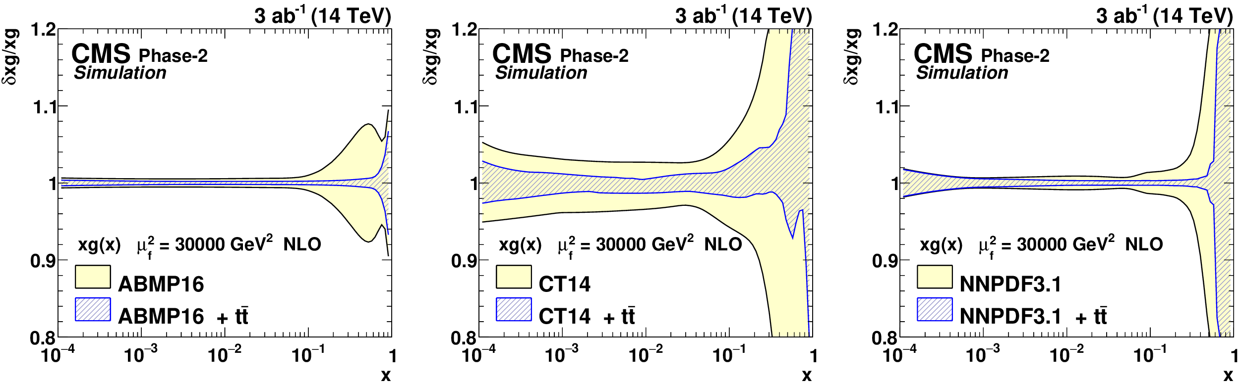
png pdf |
Figure 59:
The relative gluon PDF uncertainties of the original and profiled ABMP16 (left), CT14 (middle), and NNPDF-3.1 (right) sets. Figure taken from Ref. [297]. |
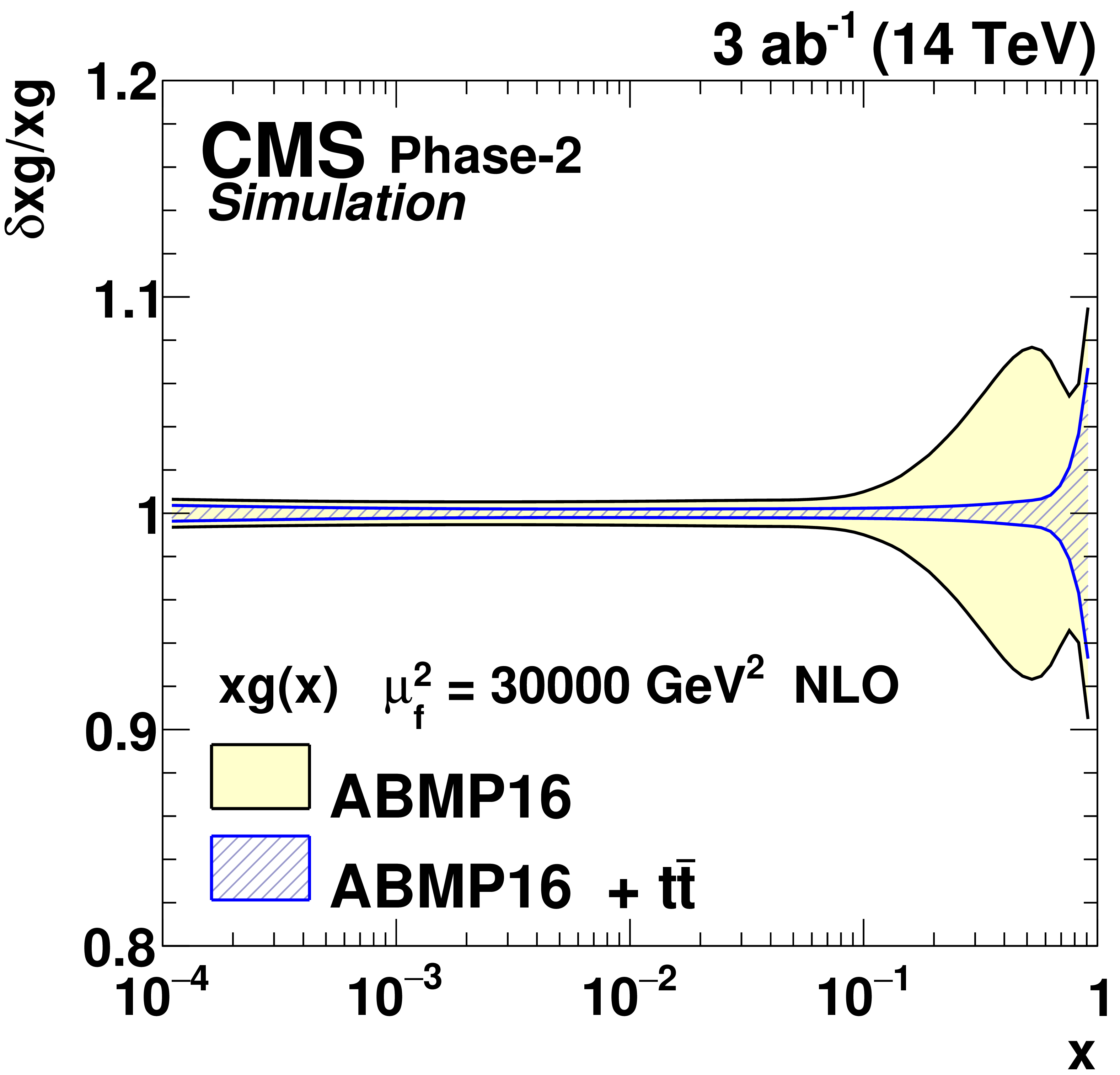
png pdf |
Figure 59-a:
The relative gluon PDF uncertainties of the original and profiled ABMP16 (left), CT14 (middle), and NNPDF-3.1 (right) sets. Figure taken from Ref. [297]. |

png pdf |
Figure 59-b:
The relative gluon PDF uncertainties of the original and profiled ABMP16 (left), CT14 (middle), and NNPDF-3.1 (right) sets. Figure taken from Ref. [297]. |
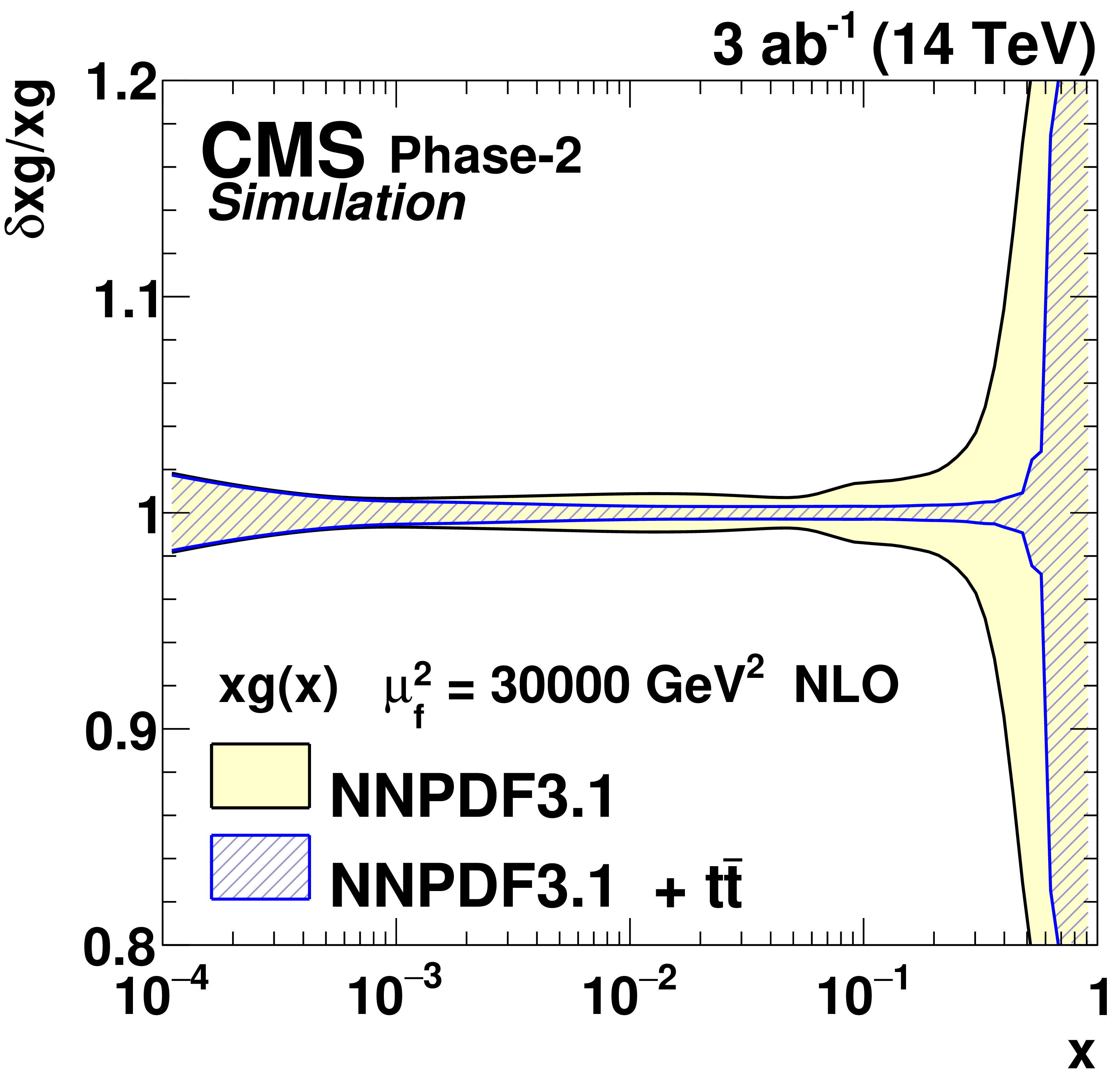
png pdf |
Figure 59-c:
The relative gluon PDF uncertainties of the original and profiled ABMP16 (left), CT14 (middle), and NNPDF-3.1 (right) sets. Figure taken from Ref. [297]. |

png pdf |
Figure 60:
Scan of the jet $ p_{\mathrm{T}} $ threshold in the measurements of the jet mass against integrated luminosity resulting in the same event yield in data after the full selection as in the most recent measurement [70]. The projection is obtained by scanning the jet $ p_{\mathrm{T}} $ spectrum observed in data. The markers correspond to 138 fb$ ^{-1} $ of LHC Run-2 data used in Ref. [70], to an estimated data set for the combination of Run-2 and Run-3, and to the HL-LHC scenario. For simplicity a constant centre-of-mass energy of 13 TeV and a similar detector acceptance to Run-2 are assumed in all scenarios. |
| Tables | |
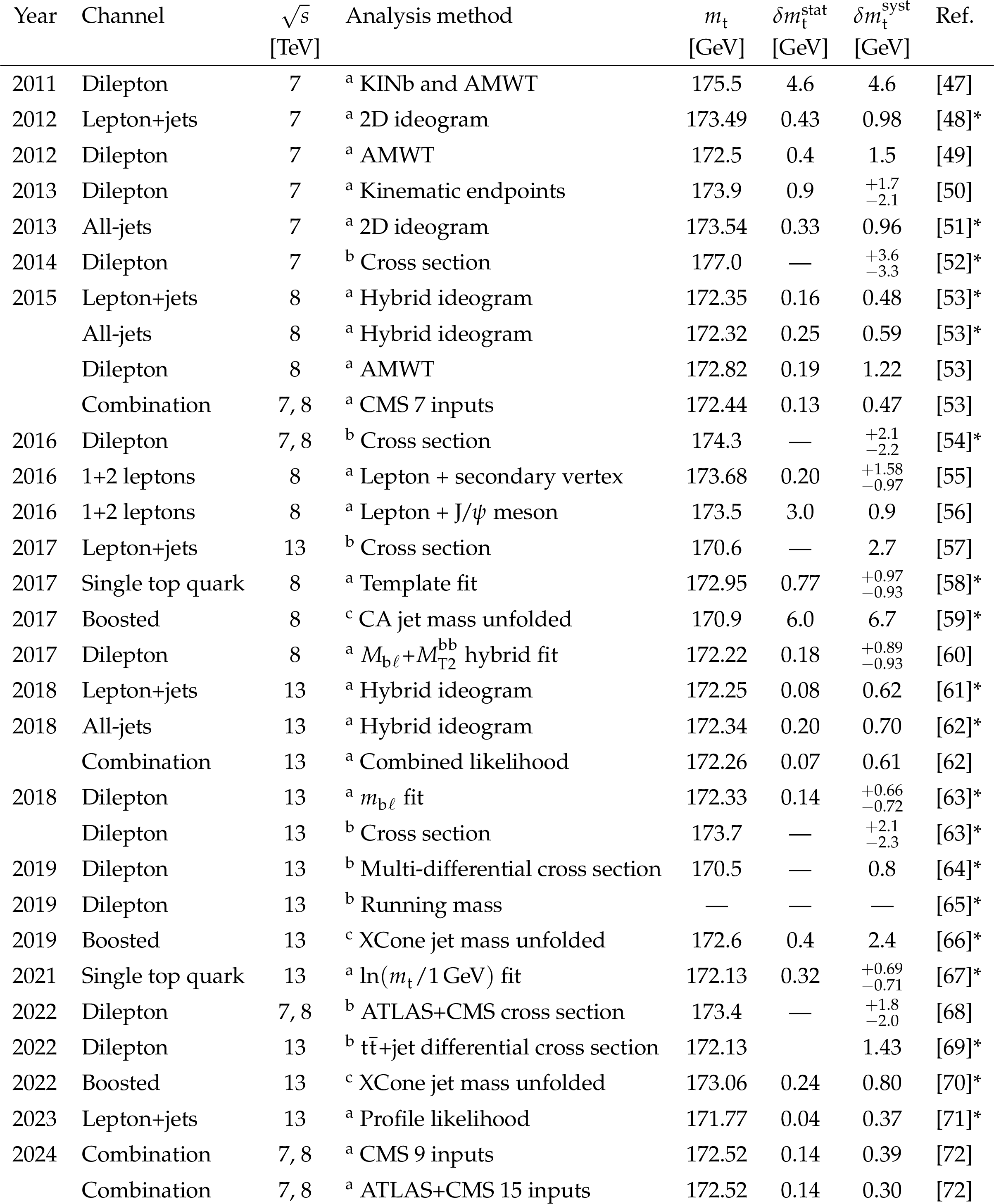
png pdf |
Table 1:
List of all CMS $ m_{\mathrm{t}} $ measurements by using different analysis methods in chronological order of publication. The summary of these measurements is also depicted in Fig. 54. The analyses are categorised as direct mass measurements (a), indirect extraction of the Lagrangian mass (b), or boosted measurements (c), as explained in the text. The analysis methods of the publications marked with a star (*) are covered in the following sections of this review. All acronyms are defined in Appendix 7. |
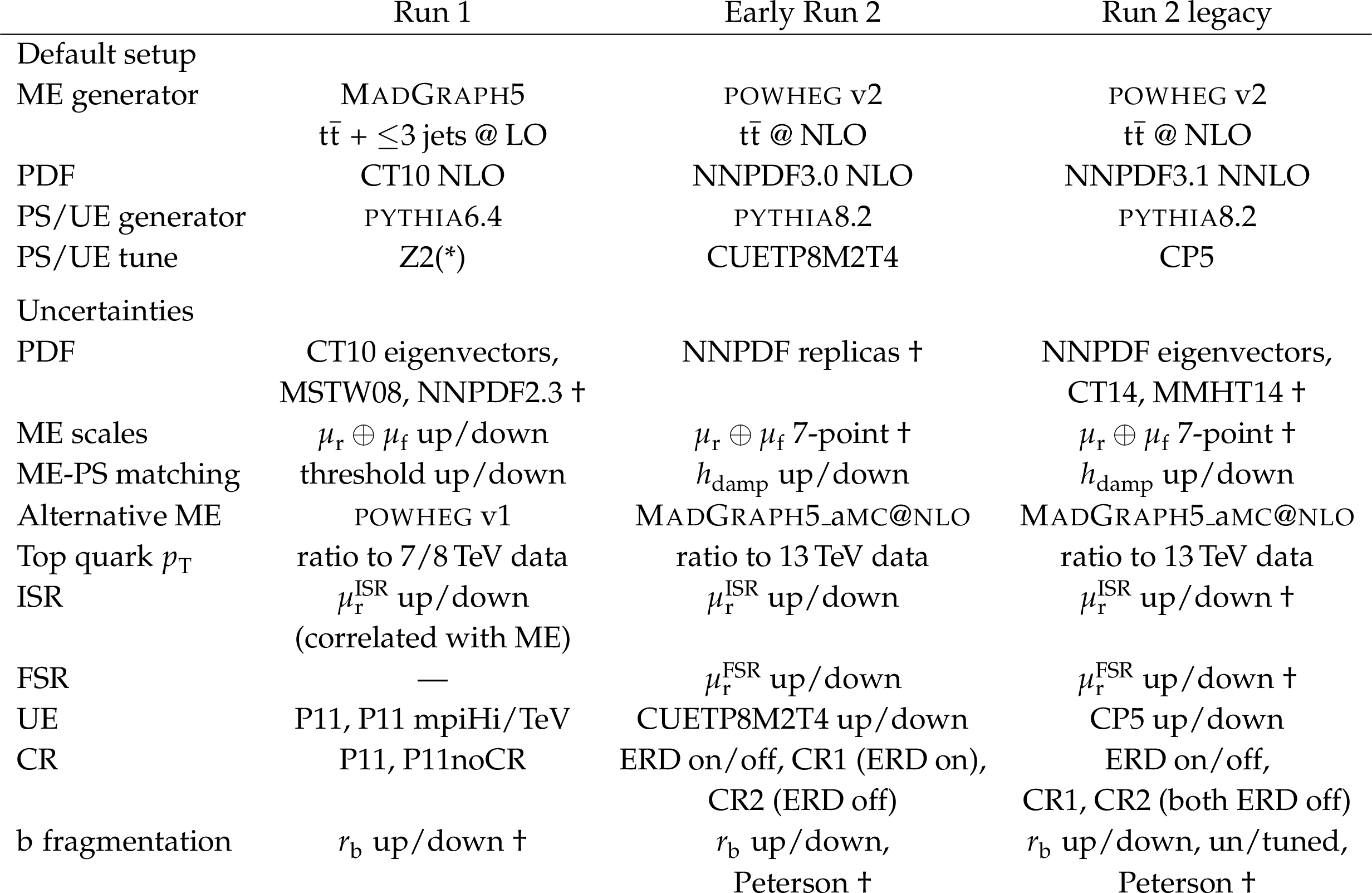
png pdf |
Table 2:
Overview of CMS MC setups for $ \mathrm{t} \overline{\mathrm{t}} $ production used in analyses of Run-1 and Run-2 data, and their associated modelling uncertainties. Variations marked with a dagger ($ \dagger $) are evaluated via event weights, which mitigates the uncertainty associated with the size of MC samples without the need for additional simulations. |
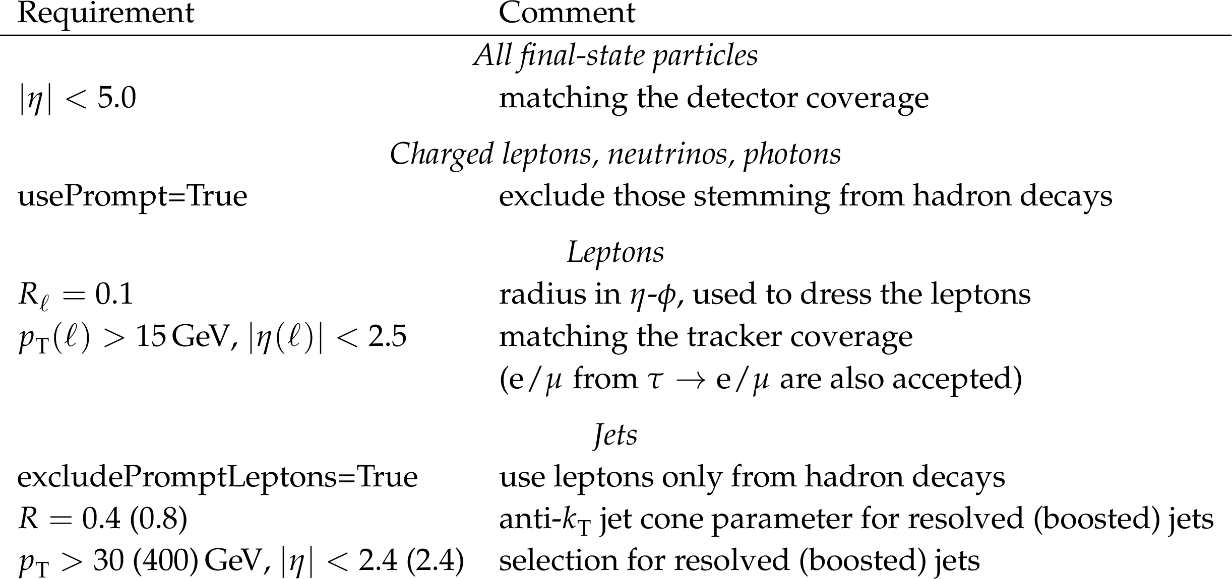
png pdf |
Table 3:
Typical object definitions, and configuration parameters used for defining top quarks at the particle level (pseudo-top candidate). The pseudo-top candidate definition is not universal and may be optimised for the production mode, final state, the variable, and the phase space being studied. The details of particle-level top quark definitions adopted in the RIVET [179,180] framework by CMS codes are described in Ref. [178] as a fundamental aspect for current and future measurements of differential production cross sections in both $ \mathrm{t} \overline{\mathrm{t}} $ and single-top quark production. |
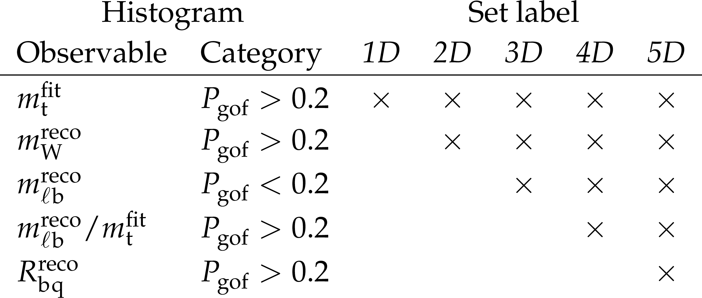
png pdf |
Table 4:
The overall list of different input histograms and their inclusion in a certain histogram set. A histogram marked with ``$ \times $'' is included in a set (measurement). |
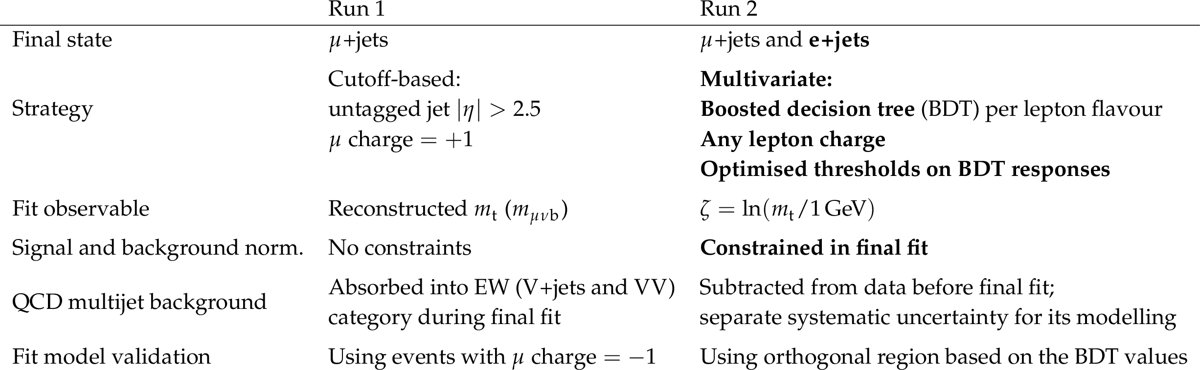
png pdf |
Table 5:
Advancement in analysis strategies between Run-1 [58] and Run-2 [67] measurements of $ m_{\mathrm{t}} $ in single top events. Primary improvements that resulted in a higher precision in the Run-2 measurement are highlighted in bold. |
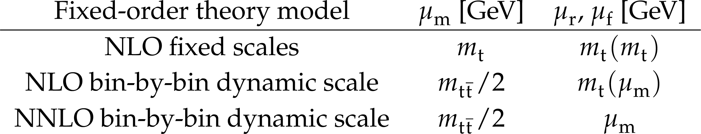
png pdf |
Table 6:
Summary of scale choices for $ \mu_{\mathrm{r}} $, $ \mu_{\mathrm{f}} $, and $ \mu_{\mathrm{m}} $ for the three different extractions of the running of the top quark mass. The NLO fixed scale corresponds to the result of Ref. [65], while the NNLO result is described in Ref. [241]. The NLO bin-by-bin dynamic result, instead, is obtained in the scope of this review work. |
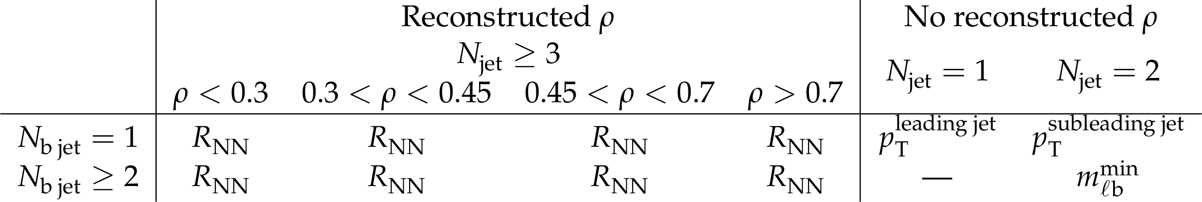
png pdf |
Table 7:
A list of the event categories and distributions used in the maximum likelihood fit. |
| Summary |
| Measurements of the top quark mass have been an essential part of the CMS research programme since the first data were recorded in 2010, with more than 20 journal publications that reveal different aspects related to this fundamental parameter of the standard model. A growing understanding of theoretical and experimental issues on the way towards increasing precision in $ m_{\mathrm{t}} $, demanded by matching the accuracy of other electroweak parameters, were followed by steady improvements in analysis techniques. Different complementary methods have been used for measurements of $ m_{\mathrm{t}} $, affected by different sources of theoretical and experimental systematic uncertainties. An impressive sub-GeV precision has been achieved, despite the challenging environment of high-energy pp collisions at the LHC, where events are affected by QCD and electroweak radiation, the underlying event and an unprecedented level of pileup interactions. This success, and a clear perspective of experimental improvements envisaged for the HL-LHC, give confidence in reaching the ultimate precision in $ m_{\mathrm{t}} $ achievable at a hadron collider in the next decade. This experimental goal requires that the necessary theoretical developments will take place, including advancements in the description of the top quark beyond the picture of a free particle, matching higher-order calculations to resummations and hadronisation models, and calculating corrections at the threshold of $ \mathrm{t} \overline{\mathrm{t}} $ production. The precise determination of $ m_{\mathrm{t}} $ is an ongoing endeavor that fosters a close collaboration of the experimental and theoretical communities, with bright prospects in the coming years. |
| References | ||||
| 1 | Particle Data Group , R. L. Workman et al. | Review of particle physics | Prog. Theor. Exp. Phys. 2022 (2022) 083C01 | |
| 2 | G. Mahlon and S. J. Parke | Spin correlation effects in top quark pair production at the LHC | PRD 81 (2010) 074024 | 1001.3422 |
| 3 | A. H. Hoang | What is the top quark mass? | Ann. Rev. Nucl. Part. Sci. 70 (2020) 225 | 2004.12915 |
| 4 | M. Kobayashi and T. Maskawa | $ {CP} $-violation in the renormalizable theory of weak interaction | Prog. Theor. Phys. 49 (1973) 652 | |
| 5 | P. H. Ginsparg, S. L. Glashow, and M. B. Wise | Top-quark mass and bottom-quark decay | PRL 50 (1983) 1415 | |
| 6 | A. J. Buras, W. Slominski, and H. Steger | $ {\mathrm{B}} $ meson decay, $ {CP} $ violation, mixing angles and the top quark mass | NPB 238 (1984) 529 | |
| 7 | JADE Collaboration | A measurement of the electroweak induced charge asymmetry in $ {\mathrm{e}^+\mathrm{e}^-\to\mathrm{b}\overline{\mathrm{b}}} $ | PLB 146 (1984) 437 | |
| 8 | S. L. Glashow, J. Iliopoulos, and L. Maiani | Weak interactions with lepton-hadron symmetry | PRD 2 (1970) 1285 | |
| 9 | B. Adeva et al. | Search for top quark and a test of models without top quark up to 38.54 GeV at PETRA | PRL 50 (1983) 799 | |
| 10 | TOPAZ Collaboration | Search for top quark in $ \mathrm{e}^+ \mathrm{e}^- $ collisions at $ \sqrt{s}= $ 52 GeV | PRL 60 (1988) 97 | |
| 11 | UA1 Collaboration | Search for new heavy quarks in proton-antiproton collisions at $ \sqrt{s}= $ 0.63 TeV | Z. Phys. C 48 (1990) 1 | |
| 12 | UA2 Collaboration | Search for top quark production at the CERN $ {\overline{\mathrm{p}}\mathrm{p}} $ collider | Z. Phys. C 46 (1990) 179 | |
| 13 | ARGUS Collaboration | Observation of $ {\mathrm{B}^0}$-$\overline{\mathrm{B}}^{0} $ mixing | PLB 192 (1987) 245 | |
| 14 | CLEO Collaboration | $ {{\mathrm{B}^0}\overline{\mathrm{B}}^{0}} $ mixing at the \PGUP4s | PRL 62 (1989) 2233 | |
| 15 | G. Altarelli and P. J. Franzini | $ {\mathrm{B}^0}-\overline{\mathrm{B}}^{0} $ mixing within and beyond the standard model | Z. Phys. C 37 (1988) 271 | |
| 16 | ALEPH Collaboration | A search for new quarks and leptons from $ \mathrm{Z^0} $ decay | PLB 236 (1990) 511 | |
| 17 | OPAL Collaboration | A search for the top and $ \mathrm{b}^{'} $ quarks in hadronic $ \mathrm{Z^0} $ decays | PLB 236 (1990) 364 | |
| 18 | ALEPH, DELPHI, L3, and OPAL Collaborations | Electroweak parameters of the $ \mathrm{Z^0} $ resonance and the standard model | PLB 276 (1992) 247 | |
| 19 | ALEPH, DELPHI, L3, and OPAL Collaborations, and LEP Electroweak Working Group | A combination of preliminary LEP electroweak measurements and constraints on the standard model | LEP Note CERN-PPE-95-172, 1995 | |
| 20 | M. Lusignoli, L. Maiani, G. Martinelli, and L. Reina | Mixing and $ {CP} $ violation in $ \mathrm{K} $- and $ {\mathrm{B}} $-mesons: a lattice QCD point of view | NPB 369 (1992) 139 | |
| 21 | A. J. Buras | A 1993 look at the lower bound on the top quark mass from $ {CP} $ violation | PLB 317 (1993) 449 | hep-ph/9307318 |
| 22 | CDF Collaboration | Observation of top quark production in $ {\overline{\mathrm{p}}\mathrm{p}} $ collisions with the Collider Detector at Fermilab | PRL 74 (1995) 2626 | hep-ex/9503002 |
| 23 | D0 Collaboration | Observation of the top quark | PRL 74 (1995) 2632 | hep-ex/9503003 |
| 24 | D0 Collaboration | Observation of single top-quark production | PRL 103 (2009) 092001 | 0903.0850 |
| 25 | CDF Collaboration | Observation of electroweak single top-quark production | PRL 103 (2009) 092002 | 0903.0885 |
| 26 | CDF and D0 Collaborations | Combination of CDF and D0 results on the mass of the top quark using up to 9.7 fb$ ^{-1} $ at the Tevatron | 1608.01881 | |
| 27 | C. Campagnari and M. Franklin | The discovery of the top quark | Rev. Mod. Phys. 69 (1997) 137 | hep-ex/9608003 |
| 28 | J. M. Flynn and L. Randall | The electromagnetic penguin contribution to $ \epsilon^\prime/\epsilon $ for large top quark mass | PLB 224 (1989) 221 | |
| 29 | G. Buchalla, A. J. Buras, and M. K. Harlander | The anatomy of $ \epsilon^\prime/\epsilon $ in the standard model | NPB 337 (1990) 313 | |
| 30 | J. Erler and M. Schott | Electroweak precision tests of the standard model after the discovery of the Higgs noson | Prog. Part. Nucl. Phys. 106 (2019) 68 | 1902.05142 |
| 31 | J. Haller et al. | Update of the global electroweak fit and constraints on two-Higgs-doublet models | EPJC 78 (2018) 675 | 1803.01853 |
| 32 | ATLAS Collaboration | A detailed map of Higgs boson interactions by the ATLAS experiment ten years after the discovery | Nature 607 (2022) 52 | 2207.00092 |
| 33 | CMS Collaboration | A portrait of the Higgs boson by the CMS experiment ten years after the discovery | Nature 607 (2022) 60 | CMS-HIG-22-001 2207.00043 |
| 34 | CMS Collaboration | Measurement of the top quark Yukawa coupling from $ \mathrm{t} \overline{\mathrm{t}} $ kinematic distributions in the dilepton final state in proton-proton collisions at $ \sqrt{s}= $ 13 TeV | PRD 102 (2020) 092013 | CMS-TOP-19-008 2009.07123 |
| 35 | G. Degrassi et al. | Higgs mass and vacuum stability in the standard model at NNLO | JHEP 08 (2012) 098 | 1205.6497 |
| 36 | S. Alekhin, A. Djouadi, and S. Moch | The top quark and Higgs boson masses and the stability of the electroweak vacuum | PLB 716 (2012) 214 | 1207.0980 |
| 37 | S. Heinemeyer, W. Hollik, G. Weiglein, and L. Zeune | Implications of LHC search results on the W boson mass prediction in the MSSM | JHEP 12 (2013) 084 | 1311.1663 |
| 38 | F. Bezrukov, M. Y. Kalmykov, B. A. Kniehl, and M. Shaposhnikov | Higgs boson mass and new physics | JHEP 10 (2012) 140 | 1205.2893 |
| 39 | D. Dunsky, L. J. Hall, and K. Harigaya | Dark matter detection, standard model parameters and intermediate scale supersymmetry | JHEP 04 (2021) 052 | 2011.12302 |
| 40 | W. Buchmuller and D. Wyler | Effective Lagrangian analysis of new interactions and flavour conservation | NPB 268 (1986) 621 | |
| 41 | G. F. Giudice, C. Grojean, A. Pomarol, and R. Rattazzi | The strongly-interacting light Higgs | JHEP 06 (2007) 045 | hep-ph/0703164 |
| 42 | B. Grzadkowski, M. Iskrzynski, M. Misiak, and J. Rosiek | Dimension-six terms in the standard model Lagrangian | JHEP 10 (2010) 085 | 1008.4884 |
| 43 | J. Gao et al. | Simultaneous CTEQ-TEA extraction of PDFs and SMEFT parameters from jet and $ \mathrm{t} \overline{\mathrm{t}} $ data | JHEP 05 (2023) 003 | 2211.01094 |
| 44 | A. J. Buras, J. Girrbach, D. Guadagnoli, and G. Isidori | On the standard model prediction for $ \mathcal{B}({{\mathrm{B}}}{s,d}\to\mu^{+}\mu^{-}) $ | EPJC 72 (2012) 2172 | 1208.0934 |
| 45 | M. Misiak et al. | Updated next-to-next-to-leading-order QCD predictions for the weak radiative $ {\mathrm{B}} $-meson decays | PRL 114 (2015) 221801 | 1503.01789 |
| 46 | M. Czakon et al. | The $ {(Q_7, Q_{1,2})} $ contribution to $ \overline{\mathrm{B}}\to\mathrm{X}_{s}\gamma $ at $ \mathcal{O}(\alpha_\mathrm{S}^2) $ | JHEP 04 (2015) 168 | 1503.01791 |
| 47 | CMS Collaboration | Measurement of the $ \mathrm{t} \overline{\mathrm{t}} $ production cross section and the top quark mass in the dilepton channel in $ {\mathrm{p}\mathrm{p}} $ collisions at $ \sqrt{s}= $ 7 TeV | JHEP 07 (2011) 049 | CMS-TOP-11-002 1105.5661 |
| 48 | CMS Collaboration | Measurement of the top-quark mass in $ \mathrm{t} \overline{\mathrm{t}} $ events with lepton+jets final states in $ {\mathrm{p}\mathrm{p}} $ collisions at $ \sqrt{s}= $ 7 TeV | JHEP 12 (2012) 105 | CMS-TOP-11-015 1209.2319 |
| 49 | CMS Collaboration | Measurement of the top-quark mass in $ \mathrm{t} \overline{\mathrm{t}} $ events with dilepton final states in $ {\mathrm{p}\mathrm{p}} $ collisions at $ \sqrt{s}= $ 7 TeV | EPJC 72 (2012) 2202 | CMS-TOP-11-016 1209.2393 |
| 50 | CMS Collaboration | Measurement of masses in the $ \mathrm{t} \overline{\mathrm{t}} $ system by kinematic endpoints in $ {\mathrm{p}\mathrm{p}} $ collisions at $ \sqrt{s}= $ 7 TeV | EPJC 73 (2013) 2494 | CMS-TOP-11-027 1304.5783 |
| 51 | CMS Collaboration | Measurement of the top-quark mass in all-jets $ \mathrm{t} \overline{\mathrm{t}} $ events in $ {\mathrm{p}\mathrm{p}} $ collisions at $ \sqrt{s}= $ 7 TeV | EPJC 74 (2014) 2758 | CMS-TOP-11-017 1307.4617 |
| 52 | CMS Collaboration | Determination of the top-quark pole mass and strong coupling constant from the $ \mathrm{t} \overline{\mathrm{t}} $ production in $ {\mathrm{p}\mathrm{p}} $ collisions at $ \sqrt{s}= $ 7 TeV | PLB 728 (2014) 496 | CMS-TOP-12-022 1307.1907 |
| 53 | CMS Collaboration | Measurement of the top quark mass using proton-proton data at $ \sqrt{s}= $ 7 and 8 TeV | PRD 93 (2016) 072004 | CMS-TOP-14-022 1509.04044 |
| 54 | CMS Collaboration | Measurement of the $ \mathrm{t} \overline{\mathrm{t}} $ production cross section in the $ {\mathrm{e}\mu} $ channel in proton-proton collisions at $ \sqrt{s}= $ 7 and 8 TeV | JHEP 08 (2016) 029 | CMS-TOP-13-004 1603.02303 |
| 55 | CMS Collaboration | Measurement of the top quark mass using charged particles in $ {\mathrm{p}\mathrm{p}} $ collisions at $ \sqrt{s}= $ 8 TeV | PRD 93 (2016) 092006 | CMS-TOP-12-030 1603.06536 |
| 56 | CMS Collaboration | Measurement of the mass of the top quark in decays with a $ \mathrm{J}/\psi $ meson in $ {\mathrm{p}\mathrm{p}} $ collisions at 8 TeV | JHEP 12 (2016) 123 | CMS-TOP-15-014 1608.03560 |
| 57 | CMS Collaboration | Measurement of the $ \mathrm{t} \overline{\mathrm{t}} $ production cross section using events with one lepton and at least one jet in $ {\mathrm{p}\mathrm{p}} $ collisions at $ \sqrt{s}= $ 13 TeV | JHEP 09 (2017) 051 | CMS-TOP-16-006 1701.06228 |
| 58 | CMS Collaboration | Measurement of the top quark mass using single top quark events in proton-proton collisions at $ \sqrt{s}= $ 8 TeV | EPJC 77 (2017) 354 | CMS-TOP-15-001 1703.02530 |
| 59 | CMS Collaboration | Measurement of the jet mass in highly boosted $ \mathrm{t} \overline{\mathrm{t}} $ events from $ {\mathrm{p}\mathrm{p}} $ collisions at $ \sqrt{s}= $ 8 TeV | EPJC 77 (2017) 467 | CMS-TOP-15-015 1703.06330 |
| 60 | CMS Collaboration | Measurement of the top quark mass in the dileptonic $ \mathrm{t} \overline{\mathrm{t}} $ decay channel using the mass observables $ {M}_{\mathrm{b}\ell} $, $ {M}_{{\mathrm{T}2}} $, and $ m_{\mathrm{b}\ell\nu} $ in $ {\mathrm{p}\mathrm{p}} $ collisions at $ \sqrt{s}= $ 8 TeV | PRD 96 (2017) 032002 | CMS-TOP-15-008 1704.06142 |
| 61 | CMS Collaboration | Measurement of the top quark mass with lepton+jets final states using $ {\mathrm{p}\mathrm{p}} $ collisions at $ \sqrt{s}= $ 13 TeV | EPJC 78 (2018) 891 | CMS-TOP-17-007 1805.01428 |
| 62 | CMS Collaboration | Measurement of the top quark mass in the all-jets final state at $ \sqrt{s}= $ 13 TeV and combination with the lepton+jets channel | EPJC 79 (2019) 313 | CMS-TOP-17-008 1812.10534 |
| 63 | CMS Collaboration | Measurement of the $ \mathrm{t} \overline{\mathrm{t}} $ production cross section, the top quark mass, and the strong coupling constant using dilepton events in $ {\mathrm{p}\mathrm{p}} $ collisions at $ \sqrt{s}= $ 13 TeV | EPJC 79 (2019) 368 | CMS-TOP-17-001 1812.10505 |
| 64 | CMS Collaboration | Measurement of $ \mathrm{t} \overline{\mathrm{t}} $ normalised multi-differential cross sections in $ {\mathrm{p}\mathrm{p}} $ collisions at $ \sqrt{s}= $ 13 TeV, and simultaneous determination of the strong coupling strength, top quark pole mass, and parton distribution functions | EPJC 80 (2020) 658 | CMS-TOP-18-004 1904.05237 |
| 65 | CMS Collaboration | Running of the top quark mass from proton-proton collisions at $ \sqrt{s}= $ 13 TeV | PLB 803 (2020) 135263 | CMS-TOP-19-007 1909.09193 |
| 66 | CMS Collaboration | Measurement of the jet mass distribution and top quark mass in hadronic decays of boosted top quarks in $ {\mathrm{p}\mathrm{p}} $ collisions at $ \sqrt{s}= $ 13 TeV | PRL 124 (2020) 202001 | CMS-TOP-19-005 1911.03800 |
| 67 | CMS Collaboration | Measurement of the top quark mass using events with a single reconstructed top quark in $ {\mathrm{p}\mathrm{p}} $ collisions at $ \sqrt{s}= $ 13 TeV | JHEP 12 (2021) 161 | CMS-TOP-19-009 2108.10407 |
| 68 | ATLAS and CMS Collaborations | Combination of inclusive top-quark pair production cross-section measurements using ATLAS and CMS data at $ \sqrt{s}= $ 7 and 8 TeV | JHEP 07 (2023) 213 | CMS-TOP-18-014 2205.13830 |
| 69 | CMS Collaboration | Measurement of the top quark pole mass using $ \mathrm{t} \overline{\mathrm{t}} $ +jet events in the dilepton final state in proton-proton collisions at $ \sqrt{s}= $ 13 TeV | JHEP 07 (2023) 077 | CMS-TOP-21-008 2207.02270 |
| 70 | CMS Collaboration | Measurement of the differential $ \mathrm{t} \overline{\mathrm{t}} $ production cross section as a function of the jet mass and extraction of the top quark mass in hadronic decays of boosted top quarks | EPJC 83 (2023) 560 | CMS-TOP-21-012 2211.01456 |
| 71 | CMS Collaboration | Measurement of the top quark mass using a profile likelihood approach with the lepton+jets final states in proton-proton collisions at $ \sqrt{s}= $ 13 TeV | EPJC 83 (2023) 963 | CMS-TOP-20-008 2302.01967 |
| 72 | ATLAS and CMS Collaborations | Combination of measurements of the top quark mass from data collected by the ATLAS and CMS experiments at $ \sqrt{s}= $ 7 and 8 TeV | Submitted to Phys. Rev. Lett, 2024 | 2402.08713 |
| 73 | CMS Collaboration | CMS physics technical design report, volume I: Detector performance and software | CMS Technical Proposal CERN-LHCC-2006-001, CMS-TDR-8.1, 2006 CDS |
|
| 74 | N. Kidonakis | NNNLO soft-gluon corrections for the top-quark $ p_{\mathrm{T}} $ and rapidity distributions | PRD 91 (2015) 031501 | 1411.2633 |
| 75 | N. Kidonakis | Top-quark double-differential distributions at approximate N3LO | PRD 101 (2020) 074006 | 1912.10362 |
| 76 | M. Czakon, D. Heymes, and A. Mitov | High-precision differential predictions for top-quark pairs at the LHC | PRL 116 (2016) 082003 | 1511.00549 |
| 77 | M. Czakon and A. Mitov | top++: a program for the calculation of the top-pair cross-section at hadron colliders | Comput. Phys. Commun. 185 (2014) 2930 | 1112.5675 |
| 78 | M. Czakon et al. | Top-pair production at the LHC through NNLO QCD and NLO EW | JHEP 10 (2017) 186 | 1705.04105 |
| 79 | M. Czakon et al. | Resummation for (boosted) top-quark pair production at NNLO+NNLL' in QCD | JHEP 05 (2018) 149 | 1803.07623 |
| 80 | S. Catani et al. | Top-quark pair production at the LHC: fully differential QCD predictions at NNLO | JHEP 07 (2019) 100 | 1906.06535 |
| 81 | M. Czakon, A. Mitov, and R. Poncelet | NNLO QCD corrections to leptonic observables in top-quark pair production and decay | JHEP 05 (2021) 212 | 2008.11133 |
| 82 | CMS Collaboration | First measurement of the top quark pair production cross section in proton-proton collisions at $ \sqrt{s}= $ 13.6 TeV | JHEP 08 (2023) 204 | CMS-TOP-22-012 2303.10680 |
| 83 | S. Cortese and R. Petronzio | The single top production channel at Tevatron energies | PLB 253 (1991) 494 | |
| 84 | S. S. D. Willenbrock and D. A. Dicus | Production of heavy quarks from W-gluon fusion | PRD 34 (1986) 155 | |
| 85 | J. Campbell, T. Neumann, and Z. Sullivan | Single-top-quark production in the $ t $-channel at NNLO | JHEP 02 (2021) 040 | 2012.01574 |
| 86 | M. Brucherseifer, F. Caola, and K. Melnikov | On the NNLO QCD corrections to single-top production at the LHC | PLB 736 (2014) 58 | 1404.7116 |
| 87 | E. L. Berger, J. Gao, and H. X. Zhu | Differential distributions for $ t $-channel single top-quark production and decay at next-to-next-to-leading order in QCD | JHEP 11 (2017) 158 | 1708.09405 |
| 88 | N. Kidonakis | Next-to-next-to-leading logarithm resummation for $ s $-channel single top quark production | PRD 81 (2010) 054028 | 1001.5034 |
| 89 | N. Kidonakis | Two-loop soft anomalous dimensions for single top quark associated production with a $ \mathrm{W^-} $ or $ \mathrm{H}^{-} $ | PRD 82 (2010) 054018 | 1005.4451 |
| 90 | M. Je \.z abek and J. H. Kühn | QCD corrections to semileptonic decays of heavy quarks | NPB 314 (1989) 1 | |
| 91 | I. Bigi et al. | Production and decay properties of ultra-heavy quarks | PLB 181 (1986) 157 | |
| 92 | CMS Collaboration | The CMS experiment at the CERN LHC | JINST 3 (2008) S08004 | |
| 93 | CMS Collaboration | Particle-flow reconstruction and global event description with the CMS detector | JINST 12 (2017) P10003 | CMS-PRF-14-001 1706.04965 |
| 94 | CMS Collaboration | Technical proposal for the Phase-II upgrade of the Compact Muon Solenoid | CMS Technical Proposal CERN-LHCC-2015-010, CMS-TDR-15-02, 2015 CDS |
|
| 95 | CMS Collaboration | Pileup removal algorithms | CMS Physics Analysis Summary, 2014 CMS-PAS-JME-14-001 |
CMS-PAS-JME-14-001 |
| 96 | CMS Collaboration | Pileup mitigation at CMS in 13 TeV data | JINST 15 (2020) P09018 | CMS-JME-18-001 2003.00503 |
| 97 | D. Bertolini, P. Harris, M. Low, and N. Tran | Pileup per particle identification | JHEP 10 (2014) 059 | 1407.6013 |
| 98 | M. Cacciari, G. P. Salam, and G. Soyez | The anti-$ k_{\mathrm{T}} $ jet clustering algorithm | JHEP 04 (2008) 063 | 0802.1189 |
| 99 | M. Cacciari, G. P. Salam, and G. Soyez | FASTJET user manual | EPJC 72 (2012) 1896 | 1111.6097 |
| 100 | CMS Collaboration | Performance of missing transverse momentum reconstruction in proton-proton collisions at $ \sqrt{s}= $ 13 TeV using the CMS detector | JINST 14 (2019) P07004 | CMS-JME-17-001 1903.06078 |
| 101 | CMS Collaboration | Jet energy scale and resolution in the CMS experiment in $ {\mathrm{p}\mathrm{p}} $ collisions at 8 TeV | JINST 12 (2017) P02014 | CMS-JME-13-004 1607.03663 |
| 102 | CMS Collaboration | Identification of heavy-flavour jets with the CMS detector in $ {\mathrm{p}\mathrm{p}} $ collisions at 13 TeV | JINST 13 (2018) P05011 | CMS-BTV-16-002 1712.07158 |
| 103 | D0 Collaboration | Direct measurement of the top quark mass at D0 | PRD 58 (1998) 052001 | hep-ex/9801025 |
| 104 | J. D'Hondt et al. | Fitting of event topologies with external kinematic constraints in CMS | CMS Note CMS-NOTE-2006-023, 2006 | |
| 105 | L. Sonnenschein | Analytical solution of $ \mathrm{t} \overline{\mathrm{t}} $ dilepton equations | PRD 73 (2006) 054015 | hep-ph/0603011 |
| 106 | S. Frixione, G. Ridolfi, and P. Nason | A positive-weight next-to-leading-order Monte Carlo for heavy flavour hadroproduction | JHEP 09 (2007) 126 | 0707.3088 |
| 107 | P. Nason | A new method for combining NLO QCD with shower Monte Carlo algorithms | JHEP 11 (2004) 040 | hep-ph/0409146 |
| 108 | S. Alioli, P. Nason, C. Oleari, and E. Re | A general framework for implementing NLO calculations in shower Monte Carlo programs: the POWHEG box | JHEP 06 (2010) 043 | 1002.2581 |
| 109 | S. Frixione, P. Nason, and C. Oleari | Matching NLO QCD computations with parton shower simulations: the POWHEG method | JHEP 11 (2007) 070 | 0709.2092 |
| 110 | T. Sjöstrand et al. | An introduction to PYTHIA8.2 | Comput. Phys. Commun. 191 (2015) 159 | 1410.3012 |
| 111 | J. Alwall et al. | MadGraph 5: going beyond | JHEP 06 (2011) 128 | 1106.0522 |
| 112 | GEANT4 Collaboration | GEANT 4---a simulation toolkit | NIM A 506 (2003) 250 | |
| 113 | Particle Data Group , W. M. Yao et al. | Review of particle physics | J. Phys. G. 33 (2006) 1 | |
| 114 | P. Artoisenet, R. Frederix, O. Mattelaer, and R. Rietkerk | Automatic spin-entangled decays of heavy resonances in Monte Carlo simulations | JHEP 03 (2013) 015 | 1212.3460 |
| 115 | T. Sjöstrand, S. Mrenna, and P. Z. Skands | PYTHIA6.4 physics and manual | JHEP 05 (2006) 026 | hep-ph/0603175 |
| 116 | CMS Collaboration | Measurement of the underlying event activity at the LHC with $ \sqrt{s}= $ 7 TeV and comparison with $ \sqrt{s}= $ 0.9 TeV | JHEP 09 (2011) 109 | CMS-QCD-10-010 1107.0330 |
| 117 | CMS Collaboration | Event generator tunes obtained from underlying event and multiparton scattering measurements | EPJC 76 (2016) 155 | CMS-GEN-14-001 1512.00815 |
| 118 | A. Buckley et al. | Systematic event generator tuning for the LHC | EPJC 65 (2010) 331 | 0907.2973 |
| 119 | CMS Collaboration | Investigations of the impact of the parton shower tuning in PYTHIA8 in the modelling of $ \mathrm{t} \overline{\mathrm{t}} $ at $ \sqrt{s}= $ 8 and 13 TeV | CMS Physics Analysis Summary, 2016 CMS-PAS-TOP-16-021 |
CMS-PAS-TOP-16-021 |
| 120 | CMS Collaboration | Extraction and validation of a new set of CMS PYTHIA8 tunes from underlying-event measurements | EPJC 80 (2020) 4 | CMS-GEN-17-001 1903.12179 |
| 121 | W. Giele et al. | The QCD/SM working group: Summary report | in Proc. 2nd Les Houches Workshop on Physics at TeV Colliders: Les Houches, France, 2001 PhysTeV 200 (2001) 275 |
hep-ph/0204316 |
| 122 | M. R. Whalley, D. Bourilkov, and R. C. Group | The Les Houches accord PDFs (LHAPDF) and LHAGLUE | in Proc. HERA and the LHC: A Workshop on the Implications of HERA and LHC Physics: Meyrin, Switzerland, 2004 March 2 (2004) 575 |
hep-ph/0508110 |
| 123 | D. Bourilkov, R. C. Group, and M. R. Whalley | LHAPDF: PDF use from the Tevatron to the LHC | in Proc. TeV4LHC Workshop, 4th Meeting: Batavia IL, USA, 2005 | hep-ph/0605240 |
| 124 | H.-L. Lai et al. | New parton distributions for collider physics | PRD 82 (2010) 074024 | 1007.2241 |
| 125 | A. D. Martin, W. J. Stirling, R. S. Thorne, and G. Watt | Parton distributions for the LHC | EPJC 63 (2009) 189 | 0901.0002 |
| 126 | NNPDF Collaboration | Parton distributions with LHC data | NPB 867 (2013) 244 | 1207.1303 |
| 127 | NNPDF Collaboration | Parton distributions for the LHC run II | JHEP 04 (2015) 040 | 1410.8849 |
| 128 | S. Dulat et al. | New parton distribution functions from a global analysis of quantum chromodynamics | PRD 93 (2016) 033006 | 1506.07443 |
| 129 | L. A. Harland-Lang, A. D. Martin, P. Motylinski, and R. S. Thorne | Parton distributions in the LHC era: MMHT 2014 PDFs | EPJC 75 (2015) 204 | 1412.3989 |
| 130 | M. Cacciari et al. | The $ \mathrm{t} \overline{\mathrm{t}} $ cross-section at 1.8 and 1.96 TeV: a study of the systematics due to parton densities and scale dependence | JHEP 04 (2004) 068 | hep-ph/0303085 |
| 131 | J. Alwall et al. | Comparative study of various algorithms for the merging of parton showers and matrix elements in hadronic collisions | EPJC 53 (2008) 473 | 0706.2569 |
| 132 | CMS Collaboration | Measurement of $ \mathrm{t} \overline{\mathrm{t}} $ production with additional jet activity, including b quark jets, in the dilepton decay channel using $ {\mathrm{p}\mathrm{p}} $ collisions at $ \sqrt{s}= $ 8 TeV | EPJC 76 (2016) 379 | CMS-TOP-12-041 1510.03072 |
| 133 | S. Mrenna and P. Skands | Automated parton-shower variations in PYTHIA8 | PRD 94 (2016) 074005 | 1605.08352 |
| 134 | CMS Collaboration | Measurements of differential cross sections of top quark pair production as a function of kinematic event variables in proton-proton collisions at $ \sqrt{s}= $ 13 TeV | JHEP 06 (2018) 002 | CMS-TOP-16-014 1803.03991 |
| 135 | CMS Collaboration | Measurement of jet substructure observables in $ \mathrm{t} \overline{\mathrm{t}} $ events from proton-proton collisions at $ \sqrt{s}= $ 13 TeV | PRD 98 (2018) 092014 | CMS-TOP-17-013 1808.07340 |
| 136 | R. Frederix and S. Frixione | Merging meets matching in MC@NLO | JHEP 12 (2012) 061 | 1209.6215 |
| 137 | S. Frixione, S. Amoroso, and S. Mrenna | Matrix element corrections in the PYTHIA8 parton shower in the context of matched simulations at next-to-leading order | EPJC 83 (2023) 970 | 2308.06389 |
| 138 | CMS Collaboration | Measurement of differential cross sections for top quark pair production using the lepton+jets final state in proton-proton collisions at 13 TeV | PRD 95 (2017) 092001 | CMS-TOP-16-008 1610.04191 |
| 139 | CMS Collaboration | Measurement of differential cross sections for the production of top quark pairs and of additional jets in lepton+jets events from $ {\mathrm{p}\mathrm{p}} $ collisions at $ \sqrt{s}= $ 13 TeV | PRD 97 (2018) 112003 | CMS-TOP-17-002 1803.08856 |
| 140 | P. Z. Skands | Tuning Monte Carlo generators: The Perugia tunes | PRD 82 (2010) 074018 | 1005.3457 |
| 141 | NNPDF Collaboration | Parton distributions from high-precision collider data | EPJC 77 (2017) 663 | 1706.00428 |
| 142 | CMS Collaboration | Pseudorapidity distribution of charged hadrons in proton-proton collisions at $ \sqrt{s}= $ 13 TeV | PLB 751 (2015) 143 | CMS-FSQ-15-001 1507.05915 |
| 143 | CMS Collaboration | Underlying event measurements with leading particles and jets in $ {\mathrm{p}\mathrm{p}} $ collisions at $ \sqrt{s}= $ 13 TeV | CMS Physics Analysis Summary, 2015 CMS-PAS-FSQ-15-007 |
CMS-PAS-FSQ-15-007 |
| 144 | CMS Collaboration | Study of the underlying event in top quark pair production in $ {\mathrm{p}\mathrm{p}} $ collisions at 13 TeV | EPJC 79 (2019) 123 | CMS-TOP-17-015 1807.02810 |
| 145 | M. H. Seymour and A. Si \'o dmok | Constraining MPI models using $ \sigma_{\text{eff}} $ and recent Tevatron and LHC underlying event data | JHEP 10 (2013) 113 | 1307.5015 |
| 146 | J. Pumplin et al. | New generation of parton distributions with uncertainties from global QCD analysis | JHEP 07 (2002) 012 | hep-ph/0201195 |
| 147 | M. Bähr et al. | HERWIG++ physics and manual | EPJC 58 (2008) 639 | 0803.0883 |
| 148 | J. Bellm et al. | HERWIG 7.0/ HERWIG++ 3.0 release note | EPJC 76 (2016) 196 | 1512.01178 |
| 149 | T. Gleisberg et al. | Event generation with SHERPA 1.1 | JHEP 02 (2009) 007 | 0811.4622 |
| 150 | F. Cascioli, P. Maierhöfer, and S. Pozzorini | Scattering amplitudes with open loops | PRL 108 (2012) 111601 | 1111.5206 |
| 151 | S. Schumann and F. Krauss | A parton shower algorithm based on Catani--Seymour dipole factorisation | JHEP 03 (2008) 038 | 0709.1027 |
| 152 | CMS Collaboration | CMS PYTHIA8 colour reconnection tunes based on underlying-event data | EPJC 83 (2023) 587 | CMS-GEN-17-002 2205.02905 |
| 153 | S. Argyropoulos and T. Sjöstrand | Effects of color reconnection on $ \mathrm{t} \overline{\mathrm{t}} $ final states at the LHC | JHEP 11 (2014) 043 | 1407.6653 |
| 154 | ATLAS Collaboration | Measurement of colour flow with the jet pull angle in $ \mathrm{t} \overline{\mathrm{t}} $ events using the ATLAS detector at $ \sqrt{s}= $ 8 TeV | PLB 750 (2015) 475 | 1506.05629 |
| 155 | M. G. Bowler | $ \mathrm{e}^+ \mathrm{e}^- $ production of heavy quarks in the string model | Z. Phys. C 11 (1981) 169 | |
| 156 | ALEPH Collaboration | Study of the fragmentation of b quarks into $ {\mathrm{B}} $ mesons at the Z peak | PLB 512 (2001) 30 | hep-ex/0106051 |
| 157 | DELPHI Collaboration | A study of the b-quark fragmentation function with the DELPHI detector at \mboxLEP I and an averaged distribution obtained at the Z pole | EPJC 71 (2011) 1557 | 1102.4748 |
| 158 | OPAL Collaboration | Inclusive analysis of the b quark fragmentation function in Z decays at LEP | EPJC 29 (2003) 463 | hep-ex/0210031 |
| 159 | SLD Collaboration | Measurement of the b-quark fragmentation function in $ \mathrm{Z^0} $ decays | PRD 65 (2002) 092006 | hep-ex/0202031 |
| 160 | C. Peterson, D. Schlatter, I. Schmitt, and P. M. Zerwas | Scaling violations in inclusive $ \mathrm{e}^+ \mathrm{e}^- $ annihilation spectra | PRD 27 (1983) 105 | |
| 161 | CMS Collaboration | Performance of the CMS missing transverse momentum reconstruction in $ {\mathrm{p}\mathrm{p}} $ data at $ \sqrt{s}= $ 8 TeV | JINST 10 (2015) P02006 | CMS-JME-13-003 1411.0511 |
| 162 | CMS Collaboration | Electron and photon reconstruction and identification with the CMS experiment at the CERN LHC | JINST 16 (2021) P05014 | CMS-EGM-17-001 2012.06888 |
| 163 | CMS Collaboration | Performance of the CMS muon detector and muon reconstruction with proton-proton collisions at $ \sqrt{s}= $ 13 TeV | JINST 13 (2018) P06015 | CMS-MUO-16-001 1804.04528 |
| 164 | CMS Collaboration | The CMS trigger system | JINST 12 (2017) P01020 | CMS-TRG-12-001 1609.02366 |
| 165 | CMS Collaboration | Absolute calibration of the luminosity measurement at CMS: Winter 2012 update | CMS Physics Analysis Summary, 2012 CMS-PAS-SMP-12-008 |
|
| 166 | CMS Collaboration | CMS luminosity based on pixel cluster counting---Summer 2013 update | CMS Physics Analysis Summary, 2013 CMS-PAS-LUM-13-001 |
CMS-PAS-LUM-13-001 |
| 167 | CMS Collaboration | Precision luminosity measurement in proton-proton collisions at $ \sqrt{s}= $ 13 TeV in 2015 and 2016 at CMS | EPJC 81 (2021) 800 | CMS-LUM-17-003 2104.01927 |
| 168 | CMS Collaboration | CMS luminosity measurement for the 2017 data-taking period at $ \sqrt{s}= $ 13 TeV | CMS Physics Analysis Summary, 2018 CMS-PAS-LUM-17-004 |
CMS-PAS-LUM-17-004 |
| 169 | CMS Collaboration | CMS luminosity measurement for the 2018 data-taking period at $ \sqrt{s}= $ 13 TeV | CMS Physics Analysis Summary, 2019 CMS-PAS-LUM-18-002 |
CMS-PAS-LUM-18-002 |
| 170 | S. Schmitt | TUnfold, an algorithm for correcting migration effects in high energy physics | JINST 7 (2012) T10003 | 1205.6201 |
| 171 | S. Schmitt | Data unfolding methods in high energy physics | in Proc. 12th Conference on Quark Confinement and the Hadron Spectrum (Confinement XII): Thessaloniki, Greece, 2017 EPJ Web Conf. 137 (2017) 11008 |
1611.01927 |
| 172 | G. D'Agostini | A multidimensional unfolding method based on Bayes' theorem | NIM A 362 (1995) 487 | |
| 173 | G. D'Agostini | Improved iterative Bayesian unfolding | in Proc. Alliance Workshop on Unfolding and Data Correction: Hamburg, Germany, 2010 | 1010.0632 |
| 174 | A. Höcker and V. Kartvelishvili | SVD approach to data unfolding | NIM A 372 (1996) 469 | hep-ph/9509307 |
| 175 | A. N. Tikhonov | On the solution of ill-posed problems and the method of regularization | Dokl. Akad. Nauk SSSR 151 (1963) 3 | |
| 176 | L. Brenner et al. | Comparison of unfolding methods using RooFitUnfold | Int. J. Mod. Phys. A 35 (2020) 2050145 | 1910.14654 |
| 177 | M. Stanley, P. Patil, and M. Kuusela | Uncertainty quantification for wide-bin unfolding: one-at-a-time strict bounds and prior-optimized confidence intervals | JINST 17 (2022) P10013 | 2111.01091 |
| 178 | CMS Collaboration | Object definitions for top quark analyses at the particle level | CMS Note CMS-NOTE-2017-004, 2017 CDS |
|
| 179 | A. Buckley et al. | RIVET user manual | Comput. Phys. Commun. 184 (2013) 2803 | 1003.0694 |
| 180 | C. Bierlich et al. | Robust independent validation of experiment and theory: RIVET version 3 | SciPost Phys. 8 (2020) 026 | 1912.05451 |
| 181 | F. Herren and M. Steinhauser | Version 3 of RunDec and CRunDec | Comput. Phys. Commun. 224 (2018) 333 | 1703.03751 |
| 182 | A. H. Hoang, C. Lepenik, and V. Mateu | REvolver: Automated running and matching of couplings and masses in QCD | Comput. Phys. Commun. 270 (2022) 108145 | 2102.01085 |
| 183 | J. Mazzitelli | NNLO study of top-quark mass renormalization scheme uncertainties in Higgs boson production | JHEP 09 (2022) 065 | 2206.14667 |
| 184 | A. H. Hoang et al. | The MSR mass and the $ \mathcal{O}({\Lambda}_{{\mathrm{QCD}}}) $ renormalon sum rule | JHEP 04 (2018) 003 | 1704.01580 |
| 185 | R. Tarrach | The pole mass in perturbative QCD | NPB 183 (1981) 384 | |
| 186 | A. S. Kronfeld | Perturbative pole mass in QCD | PRD 58 (1998) 051501 | hep-ph/9805215 |
| 187 | M. Beneke, P. Marquard, P. Nason, and M. Steinhauser | On the ultimate uncertainty of the top quark pole mass | PLB 775 (2017) 63 | 1605.03609 |
| 188 | A. H. Hoang, C. Lepenik, and M. Preisser | On the light massive flavor dependence of the large order asymptotic behavior and the ambiguity of the pole mass | JHEP 09 (2017) 099 | 1706.08526 |
| 189 | A. H. Hoang, S. Mantry, A. Pathak, and I. W. Stewart | Extracting a short distance top mass with light grooming | PRD 100 (2019) 074021 | 1708.02586 |
| 190 | B. Bachu et al. | Boosted top quarks in the peak region with N3LL resummation | PRD 104 (2021) 014026 | 2012.12304 |
| 191 | A. H. Hoang, S. Plätzer, and D. Samitz | On the cutoff dependence of the quark mass parameter in angular ordered parton showers | JHEP 10 (2018) 200 | 1807.06617 |
| 192 | DELPHI Collaboration | Measurement of the mass and width of the W boson in $ \mathrm{e}^+ \mathrm{e}^- $ collisions at $ \sqrt{s}= $ 161--209 GeV | EPJC 55 (2008) 1 | 0803.2534 |
| 193 | R. Barlow and C. Beeston | Fitting using finite Monte Carlo samples | Comput. Phys. Commun. 77 (1993) 219 | |
| 194 | J. S. Conway | Incorporating nuisance parameters in likelihoods for multisource spectra | in Proc. 2011 Workshop on Statistical Issues Related to Discovery Claims in Search Experiments and Unfolding (PHYSTAT ): Geneva, Switzerland, 2011 link |
1103.0354 |
| 195 | ATLAS Collaboration | Measurement of the top quark mass in the $ {\mathrm{t}\overline{\mathrm{t}}} \to $dilepton channel from $ \sqrt{s}= $ 8 TeV | PLB 761 (2016) 350 | 1606.02179 |
| 196 | ATLAS Collaboration | Measurement of the top quark mass in the $ {\mathrm{t}\overline{\mathrm{t}}} \to $lepton+jets and $ {\mathrm{t}\overline{\mathrm{t}}} \to $dilepton channels using $ \sqrt{s}= $ 7 TeV ATLAS data | EPJC 75 (2015) 330 | 1503.05427 |
| 197 | ATLAS Collaboration | Measurement of the top quark mass in the $ {\mathrm{t}\overline{\mathrm{t}}} \to $lepton+jets channel from $ \sqrt{s}= $ 8 TeV ATLAS data and combination with previous results | EPJC 79 (2019) 290 | 1810.01772 |
| 198 | M. Aliev et al. | hathor: Hadronic top and heavy quarks cross section calculator | Comput. Phys. Commun. 182 (2011) 1034 | 1007.1327 |
| 199 | P. Kant et al. | hathor for single top-quark production: Updated predictions and uncertainty estimates for single top-quark production in hadronic collisions | Comput. Phys. Commun. 191 (2015) 74 | 1406.4403 |
| 200 | CMS Collaboration | Measurement of the single top quark and antiquark production cross sections in the $ t $ channel and their ratio in proton-proton collisions at $ \sqrt{s}= $ 13 TeV | PLB 800 (2020) 135042 | CMS-TOP-17-011 1812.10514 |
| 201 | S. Alioli, P. Nason, C. Oleari, and E. Re | NLO single-top production matched with shower in POWHEG: $ s $- and $ t $-channel contributions | JHEP 09 (2009) 111 | 0907.4076 |
| 202 | R. Frederix, E. Re, and P. Torrielli | Single-top $ t $-channel hadroproduction in the four-flavors scheme with POWHEG and aMC@NLO | JHEP 09 (2012) 130 | 1207.5391 |
| 203 | ATLAS Collaboration | Fiducial, total and differential cross-section measurements of $ t $-channel single top-quark production in $ {\mathrm{p}\mathrm{p}} $ collisions at 8 TeV using data collected by the ATLAS detector | EPJC 77 (2017) 531 | 1702.02859 |
| 204 | CMS Collaboration | Measurement of differential cross sections and charge ratios for $ t $-channel single top quark production in proton-proton collisions at $ \sqrt{s}= $ 13 TeV | EPJC 80 (2020) 370 | CMS-TOP-17-023 1907.08330 |
| 205 | M. J. Oreglia | A study of the reactions $ {\psi^\prime\to\gamma\gamma\psi} $ | PhD thesis, Stanford University, SLAC-R-236, 1980 link |
|
| 206 | Belle Collaboration | A detailed test of the CsI(T\ell) calorimeter for BELLE with photon beams of energy between 20 MeV and 5.4 GeV | NIM A 441 (2000) 401 | |
| 207 | CMS Collaboration | Determination of jet energy calibration and transverse momentum resolution in CMS | JINST 6 (2011) P11002 | CMS-JME-10-011 1107.4277 |
| 208 | O. W. Greenberg | $ {CPT} $ violation implies violation of Lorentz invariance | PRL 89 (2002) 231602 | hep-ph/0201258 |
| 209 | CMS Collaboration | Measurement of the mass difference between top and antitop quarks | JHEP 06 (2012) 109 | CMS-TOP-11-019 1204.2807 |
| 210 | CMS Collaboration | Measurement of the mass difference between top quark and antiquark in $ {\mathrm{p}\mathrm{p}} $ collisions at $ \sqrt{s}= $ 8 TeV | PLB 770 (2017) 50 | CMS-TOP-12-031 1610.09551 |
| 211 | BASE Collaboration | A 16-parts-per-trillion measurement of the antiproton-to-proton charge-mass ratio | Nature 601 (2022) 53 | |
| 212 | T. Cheng, M. Lindner, and M. Sen | Implications of a matter-antimatter mass asymmetry in Penning-trap experiments | PLB 844 (2023) 138068 | 2210.10819 |
| 213 | P. Azzi et al. | Report from working group 1: Standard model physics at the HL-LHC and HE-LHC | CERN Report CERN-LPCC-2018-03, 2019 link |
1902.04070 |
| 214 | A. H. Hoang and I. W. Stewart | Top mass measurements from jets and the Tevatron top-quark mass | in Proc. 2nd International Workshop on Top-Quark Physics (TOP): La Biodola, Italy, 2008 Nucl. Phys. B Proc. Suppl. 185 (2008) 220 |
0808.0222 |
| 215 | A. H. Hoang | The top mass: interpretation and theoretical uncertainties | in Proc. 7th International Workshop on Top Quark Physics (TOP): Cannes, France, 2014 | 1412.3649 |
| 216 | R. Baumeister and S. Weinzierl | Cutoff dependence of the thrust peak position in the dipole shower | EPJC 80 (2020) 843 | 2004.01657 |
| 217 | S. Makarov, K. Melnikov, P. Nason, and M. A. Ozcelik | Linear power corrections to top quark pair production in hadron collisions | JHEP 01 (2024) 074 | 2308.05526 |
| 218 | J. Kieseler, K. Lipka, and S.-O. Moch | Calibration of the top-quark Monte Carlo mass | PRL 116 (2016) 162001 | 1511.00841 |
| 219 | M. Butenschoen et al. | Top quark mass calibration for Monte Carlo event generators | PRL 117 (2016) 232001 | 1608.01318 |
| 220 | S. Fleming, A. H. Hoang, S. Mantry, and I. W. Stewart | Jets from massive unstable particles: Top-mass determination | PRD 77 (2008) 074010 | hep-ph/0703207 |
| 221 | S. Fleming, A. H. Hoang, S. Mantry, and I. W. Stewart | Top jets in the peak region: Factorization analysis with next-to-leading-log resummation | PRD 77 (2008) 114003 | 0711.2079 |
| 222 | ATLAS Collaboration | Towards a precise interpretation for the top quark mass parameter in ATLAS Monte Carlo samples | ATLAS PUB Note ATL-PHYS-PUB-2021-034, 2021 | |
| 223 | D. Krohn, J. Thaler, and L.-T. Wang | Jet trimming | JHEP 02 (2010) 084 | 0912.1342 |
| 224 | A. H. Hoang, S. Mantry, A. Pathak, and I. W. Stewart | Nonperturbative corrections to soft drop jet mass | JHEP 12 (2019) 002 | 1906.11843 |
| 225 | B. Dehnadi, A. H. Hoang, O. L. Jin, and V. Mateu | Top quark mass calibration for Monte Carlo event generators---an update | JHEP 12 (2023) 065 | 2309.00547 |
| 226 | D0 Collaboration | Determination of the pole and $ \overline{\mathrm{MS}} $ masses of the top quark from the $ \mathrm{t} \overline{\mathrm{t}} $ cross section | PLB 703 (2011) 422 | 1104.2887 |
| 227 | CMS Collaboration | Measurement and QCD analysis of double-differential inclusive jet cross sections in proton-proton collisions at $ \sqrt{s}= $ 13 TeV | JHEP 02 (2022) 142 | CMS-SMP-20-011 2111.10431 |
| 228 | S. Biswas, K. Melnikov, and M. Schulze | Next-to-leading order QCD effects and the top quark mass measurements at the LHC | JHEP 08 (2010) 048 | 1006.0910 |
| 229 | CMS Collaboration | Measurement of the $ \mathrm{t} \overline{\mathrm{t}} $ production cross section in the dilepton channel in $ {\mathrm{p}\mathrm{p}} $ collisions at $ \sqrt{s}= $ 7 TeV | JHEP 11 (2012) 067 | CMS-TOP-11-005 1208.2671 |
| 230 | K. Melnikov and M. Schulze | NLO QCD corrections to top quark pair production and decay at hadron colliders | JHEP 08 (2009) 049 | 0907.3090 |
| 231 | W. Bernreuther and Z.-G. Si | Distributions and correlations for top quark pair production and decay at the Tevatron and LHC | NPB 837 (2010) 90 | 1003.3926 |
| 232 | S. Moch et al. | High precision fundamental constants at the TeVns scale | 1405.4781 | |
| 233 | G. Heinrich et al. | NLO QCD corrections to $ {\mathrm{W^+}\mathrm{W^-}\mathrm{b}\overline{\mathrm{b}}} $ production with leptonic decays in the light of top quark mass and asymmetry measurements | JHEP 06 (2014) 158 | 1312.6659 |
| 234 | M. Dowling and S.-O. Moch | Differential distributions for top-quark hadro-production with a running mass | EPJC 74 (2014) 3167 | 1305.6422 |
| 235 | S. Alekhin et al. | HERAFitter: Open source QCD fit project | EPJC 75 (2015) 304 | 1410.4412 |
| 236 | P. A. Baikov, K. G. Chetyrkin, and J. H. Kühn | Quark mass and field anomalous dimensions to $ \mathcal{O}({\alpha_\mathrm{S}}^5) $ | JHEP 10 (2014) 076 | 1402.6611 |
| 237 | T. Luthe, A. Maier, P. Marquard, and Y. Schröder | Five-loop quark mass and field anomalous dimensions for a general gauge group | JHEP 01 (2017) 081 | 1612.05512 |
| 238 | L. Mihaila | Precision calculations in supersymmetric theories | Adv. High Energy Phys. 2013 (2013) 607807 | 1310.6178 |
| 239 | N. D. Christensen and R. Shrock | Implications of dynamical generation of standard-model fermion masses | PRL 94 (2005) 241801 | hep-ph/0501294 |
| 240 | S. Catani et al. | Top-quark pair hadroproduction at NNLO: differential predictions with the $ \overline{\mathrm{MS}} $ mass | JHEP 08 (2020) 027 | 2005.00557 |
| 241 | M. M. Defranchis, J. Kieseler, K. Lipka, and J. Mazzitelli | Running of the top quark mass at NNLO in QCD | 2208.11399 | |
| 242 | CMS Collaboration | Measurement of the inclusive $ \mathrm{t} \overline{\mathrm{t}} $ cross section in $ {\mathrm{p}\mathrm{p}} $ collisions at $ \sqrt{s}= $ 5.02 TeV using final states with at least one charged lepton | JHEP 03 (2018) 115 | CMS-TOP-16-023 1711.03143 |
| 243 | H1 and ZEUS Collaborations | Combination of measurements of inclusive deep inelastic $ {\mathrm{e}^\pm\mathrm{p}} $ scattering cross sections and QCD analysis of HERA data | EPJC 75 (2015) 580 | 1506.06042 |
| 244 | CMS Collaboration | Measurement of the differential cross section and charge asymmetry for inclusive $ {\mathrm{p}\mathrm{p}\to\mathrm{W}^{\pm}+\mathrm{X}} $ production at $ \sqrt{s}= $ 8 TeV | EPJC 76 (2016) 469 | CMS-SMP-14-022 1603.01803 |
| 245 | M. Guzzi, K. Lipka, and S.-O. Moch | Top-quark pair production at hadron colliders: differential cross section and phenomenological applications with DiffTop | JHEP 01 (2015) 082 | 1406.0386 |
| 246 | CMS Collaboration | Measurement of double-differential cross sections for top quark pair production in $ {\mathrm{p}\mathrm{p}} $ collisions at $ \sqrt{s}= $ 8 TeV and impact on parton distribution functions | EPJC 77 (2017) 459 | CMS-TOP-14-013 1703.01630 |
| 247 | S. Alioli et al. | A new observable to measure the top-quark mass at hadron colliders | EPJC 73 (2013) 2438 | 1303.6415 |
| 248 | M. L. Mangano, P. Nason, and G. Ridolfi | Heavy-quark correlations in hadron collisions at next-to-leading order | NPB 373 (1992) 295 | |
| 249 | S. Dittmaier, P. Uwer, and S. Weinzierl | NLO QCD corrections to $ {\mathrm{t}\overline{\mathrm{t}}} + $jet production at hadron colliders | PRL 98 (2007) 262002 | hep-ph/0703120 |
| 250 | G. Bevilacqua, M. Czakon, C. G. Papadopoulos, and M. Worek | Dominant QCD backgrounds in Higgs boson analyses at the LHC: A study of $ {\mathrm{p}\mathrm{p}}\to{\mathrm{t}\overline{\mathrm{t}}} + $ 2 jets at next-to-leading order | PRL 104 (2010) 162002 | 1002.4009 |
| 251 | G. Bevilacqua, M. Czakon, C. G. Papadopoulos, and M. Worek | Hadronic top-quark pair production in association with two jets at next-to-leading order QCD | PRD 84 (2011) 114017 | 1108.2851 |
| 252 | Particle Data Group , M. Tanabashi et al. | Review of particle physics | PRD 98 (2018) 030001 | |
| 253 | Y. Kiyo et al. | Top-quark pair production near threshold at LHC | EPJC 60 (2009) 375 | 0812.0919 |
| 254 | J. Piclum and C. Schwinn | Soft-gluon and Coulomb corrections to hadronic top-quark pair production beyond NNLO | JHEP 03 (2018) 164 | 1801.05788 |
| 255 | T. Mäkelä, A. Hoang, K. Lipka, and S.-O. Moch | Investigation of the scale dependence in the MSR and $ \overline{\mathrm{MS}} $ top quark mass schemes for the $ \mathrm{t} \overline{\mathrm{t}} $ invariant mass differential cross section using LHC data | JHEP 09 (2023) 037 | 2301.03546 |
| 256 | S. Alioli, S.-O. Moch, and P. Uwer | Hadronic top-quark pair-production with one jet and parton showering | JHEP 01 (2012) 137 | 1110.5251 |
| 257 | S. Alekhin, J. Blümlein, and S. Moch | NLO PDFs from the ABMP16 fit | EPJC 78 (2018) 477 | 1803.07537 |
| 258 | T.-J. Hou et al. | Progress in the CTEQ-TEA NNLO global QCD analysis | 1908.11394 | |
| 259 | S. Alioli et al. | Phenomenology of $ {\mathrm{t}\overline{\mathrm{t}}} {\mathrm{j}}+{\mathrm{X}} $ production at the LHC | JHEP 05 (2022) 146 | 2202.07975 |
| 260 | A. Babaev et al. | Impact of beam-beam effects on absolute luminosity calibrations at the CERN Large Hadron Collider | EPJC 84 (2024) 17 | 2306.10394 |
| 261 | A. H. Hoang et al. | Top-antitop pair production close to threshold: Synopsis of recent NNLO results | in Proc. 4th Workshop of the 2nd ECFA/DESY Study on Physics and Detectors for a Linear Electron-Positron Collider: Oxford, UK, 2000 link |
hep-ph/0001286 |
| 262 | K. Hagiwara, Y. Sumino, and H. Yokoya | Bound-state effects on top quark production at hadron colliders | PLB 666 (2008) 71 | 0804.1014 |
| 263 | W.-L. Ju et al. | Top quark pair production near threshold: single/double distributions and mass determination | JHEP 06 (2020) 158 | 2004.03088 |
| 264 | D. Britzger, K. Rabbertz, F. Stober, and M. Wobisch | New features in version 2 of the fastNLO project | fastNLO Collaboration, in Proc. 20th International Workshop on Deep-Inelastic Scattering and Related Subjects (DIS): Bonn, Germany, 2012 link |
1208.3641 |
| 265 | T. Carli et al. | A posteriori inclusion of parton density functions in NLO QCD final-state calculations at hadron colliders: the APPLGRID project | EPJC 66 (2010) 503 | 0911.2985 |
| 266 | D. Britzger et al. | NNLO interpolation grids for jet production at the LHC | EPJC 82 (2022) 930 | 2207.13735 |
| 267 | A. L. Kataev and V. S. Molokoedov | Notes on interplay between the QCD and EW perturbative corrections to the pole-running-to-top-quark mass ratio | JETP Lett. 115 (2022) 704 | 2201.12073 |
| 268 | S. Dittmaier and H. Rzehak | Electroweak renormalization based on gauge-invariant vacuum expectation values of non-linear Higgs representations. Part I. Standard model | JHEP 05 (2022) 125 | 2203.07236 |
| 269 | G. P. Salam | Towards jetography | EPJC 67 (2010) 637 | 0906.1833 |
| 270 | M. Dasgupta, A. Fregoso, S. Marzani, and G. P. Salam | Towards an understanding of jet substructure | JHEP 09 (2013) 029 | 1307.0007 |
| 271 | R. Kogler | Advances in jet substructure at the LHC: Algorithms, measurements and searches for new physical phenomena | Springer Cham, 2021 ISBN 978-3-030-72858-8 |
|
| 272 | A. J. Larkoski, I. Moult, and B. Nachman | Jet substructure at the Large Hadron Collider: A review of recent advances in theory and machine learning | Phys. Rept. 841 (2020) 1 | 1709.04464 |
| 273 | R. Kogler et al. | Jet substructure at the Large Hadron Collider | Rev. Mod. Phys. 91 (2019) 045003 | 1803.06991 |
| 274 | CMS Collaboration | Measurements of the differential jet cross section as a function of the jet mass in dijet events from proton-proton collisions at $ \sqrt{s}= $ 13 TeV | JHEP 11 (2018) 113 | CMS-SMP-16-010 1807.05974 |
| 275 | C. W. Bauer, S. Fleming, and M. E. Luke | Summing Sudakov logarithms in $ {{\mathrm{B}}\to\mathrm{X}_{\mathrm{s}}\gamma} $ in effective field theory | PRD 63 (2000) 014006 | hep-ph/0005275 |
| 276 | C. W. Bauer, S. Fleming, D. Pirjol, and I. W. Stewart | An effective field theory for collinear and soft gluons: Heavy to light decays | PRD 63 (2001) 114020 | hep-ph/0011336 |
| 277 | C. W. Bauer and I. W. Stewart | Invariant operators in collinear effective theory | PLB 516 (2001) 134 | hep-ph/0107001 |
| 278 | C. W. Bauer, D. Pirjol, and I. W. Stewart | Soft-collinear factorization in effective field theory | PRD 65 (2002) 054022 | hep-ph/0109045 |
| 279 | C. W. Bauer et al. | Hard scattering factorization from effective field theory | PRD 66 (2002) 014017 | hep-ph/0202088 |
| 280 | A. J. Larkoski, S. Marzani, G. Soyez, and J. Thaler | Soft drop | JHEP 05 (2014) 146 | 1402.2657 |
| 281 | I. W. Stewart et al. | XCone: $ {N} $-jettiness as an exclusive cone jet algorithm | JHEP 11 (2015) 072 | 1508.01516 |
| 282 | Y. L. Dokshitzer, G. D. Leder, S. Moretti, and B. R. Webber | Better jet clustering algorithms | JHEP 08 (1997) 001 | hep-ph/9707323 |
| 283 | M. Wobisch and T. Wengler | Hadronization corrections to jet cross sections in deep-inelastic scattering | in Proc. Workshop on Monte Carlo Generators for HERA Physics: Hamburg, Germany, 1998 | hep-ph/9907280 |
| 284 | J. Thaler and T. F. Wilkason | Resolving boosted jets with XCone | JHEP 12 (2015) 051 | 1508.01518 |
| 285 | I. W. Stewart, F. J. Tackmann, and W. J. Waalewijn | $ {N} $ jettiness: An inclusive event shape to veto jets | PRL 105 (2010) 092002 | 1004.2489 |
| 286 | J. Thaler and K. Van Tilburg | Identifying boosted objects with $ {N} $-subjettiness | JHEP 03 (2011) 015 | 1011.2268 |
| 287 | J. Thaler and K. Van Tilburg | Maximizing boosted top identification by minimizing $ {N} $-subjettiness | JHEP 02 (2012) 093 | 1108.2701 |
| 288 | G. Apollinari et al. | High-Luminosity Large Hadron Collider (HL-LHC): Preliminary design report | CERN Technical Proposal CERN-2015-005, 2015 link |
|
| 289 | CMS Collaboration | The Phase-2 upgrade of the CMS tracker | CMS Technical Proposal CERN-LHCC-2017-009, CMS-TDR-014, 2017 link |
|
| 290 | CMS Collaboration | The Phase-2 upgrade of the CMS muon detectors | CMS Technical Proposal CERN-LHCC-2017-012, CMS-TDR-016, 2017 CDS |
|
| 291 | CMS Collaboration | A MIP timing detector for the CMS Phase-2 upgrade | CMS Technical Proposal CERN-LHCC-2019-003, CMS-TDR-020, 2019 CDS |
|
| 292 | CMS Collaboration | The Phase-2 upgrade of the CMS endcap calorimeter | CMS Technical Proposal CERN-LHCC-2017-023, CMS-TDR-019, 2017 CDS |
|
| 293 | CMS Collaboration | The Phase-2 upgrade of the CMS barrel calorimeters | CMS Technical Proposal CERN-LHCC-2017-011, CMS-TDR-015, 2017 CDS |
|
| 294 | CMS Collaboration | ECFA 2016: Prospects for selected standard model measurements with the CMS experiment at the High-Luminosity LHC | CMS Physics Analysis Summary, 2017 CMS-PAS-FTR-16-006 |
CMS-PAS-FTR-16-006 |
| 295 | CMS Collaboration | Expected performance of the physics objects with the upgraded CMS detector at the HL-LHC | CMS Note CMS-NOTE-2018-006, 2018 CDS |
|
| 296 | CMS Collaboration | The Phase-2 upgrade of the CMS beam radiation, instrumentation, and luminosity detectors | CMS Technical Proposal CERN-LHCC-2021-008, CMS-TDR-023, 2021 CDS |
|
| 297 | A. Dainese et al. | Physics at the HL-LHC, and perspectives at the HE-LHC | CERN Report CERN-2019-007, 2019 link |
|
| 298 | H. Paukkunen and P. Zurita | PDF reweighting in the Hessian matrix approach | JHEP 12 (2014) 100 | 1402.6623 |
|
|
Compact Muon Solenoid LHC, CERN |
|

|

|

|

|

|