

Compact Muon Solenoid
LHC, CERN
| CMS-EXO-23-007 ; CERN-EP-2024-068 | ||
| Enriching the physics program of the CMS experiment via data scouting and data parking | ||
| CMS Collaboration | ||
| 24 March 2024 | ||
| To be submitted | ||
| Abstract: Specialized data-taking and data-processing techniques were introduced by the CMS experiment in Run 1 of the CERN LHC to enhance the sensitivity of searches for new physics and the precision of standard model measurements. These techniques, termed data scouting and data parking, extend the data-taking capabilities of CMS beyond the original design specifications. The novel data-scouting strategy trades complete event information for higher event rates, while keeping the data bandwidth within limits. Data parking involves storing a large amount of raw detector data collected by algorithms with low trigger thresholds to be processed when sufficient computational power is available to handle such data. The research program of the CMS Collaboration is greatly expanded with these techniques. The implementation, performance, and physics results obtained with data scouting and data parking in CMS over the last decade are discussed in this Report, along with new developments aimed at further improving low-mass physics sensitivity over the next years of data taking. | ||
| Links: e-print arXiv:2403.16134 [hep-ex] (PDF) ; CDS record ; inSPIRE record ; Physics Briefing ; CADI line (restricted) ; | ||
| Figures | |
png pdf |
Figure 1:
A schematic view of the typical Run 2 data flow during 2018 showing the data acquisition strategy with scouting and parking data streams, along with the standard data stream. A value of $ {\mathcal{L}_{\text{inst}}} = $ 1.2 $\times$ 10$^{34}$ cm$^{-2}$s$^{-1}$ over a typical 2018 fill, corresponding to an average pileup of 38, is considered. |
png pdf |
Figure 2:
Comparison of the typical HLT rates of the standard, parking, and scouting data streams from Run 1 to Run 3. The $ \mathcal{L}_{\text{inst}} $ averaged over one typical fill of a given data-taking year is shown in pink. |
png pdf |
Figure 3:
The efficiency of the Run 2 Calo scouting (left) and standard (right) jet triggers as a function of the reconstructed mass of the dijet system. Figures taken from Ref. [65]. |

png pdf |
Figure 3-a:
The efficiency of the Run 2 Calo scouting (left) and standard (right) jet triggers as a function of the reconstructed mass of the dijet system. Figures taken from Ref. [65]. |

png pdf |
Figure 3-b:
The efficiency of the Run 2 Calo scouting (left) and standard (right) jet triggers as a function of the reconstructed mass of the dijet system. Figures taken from Ref. [65]. |
png pdf |
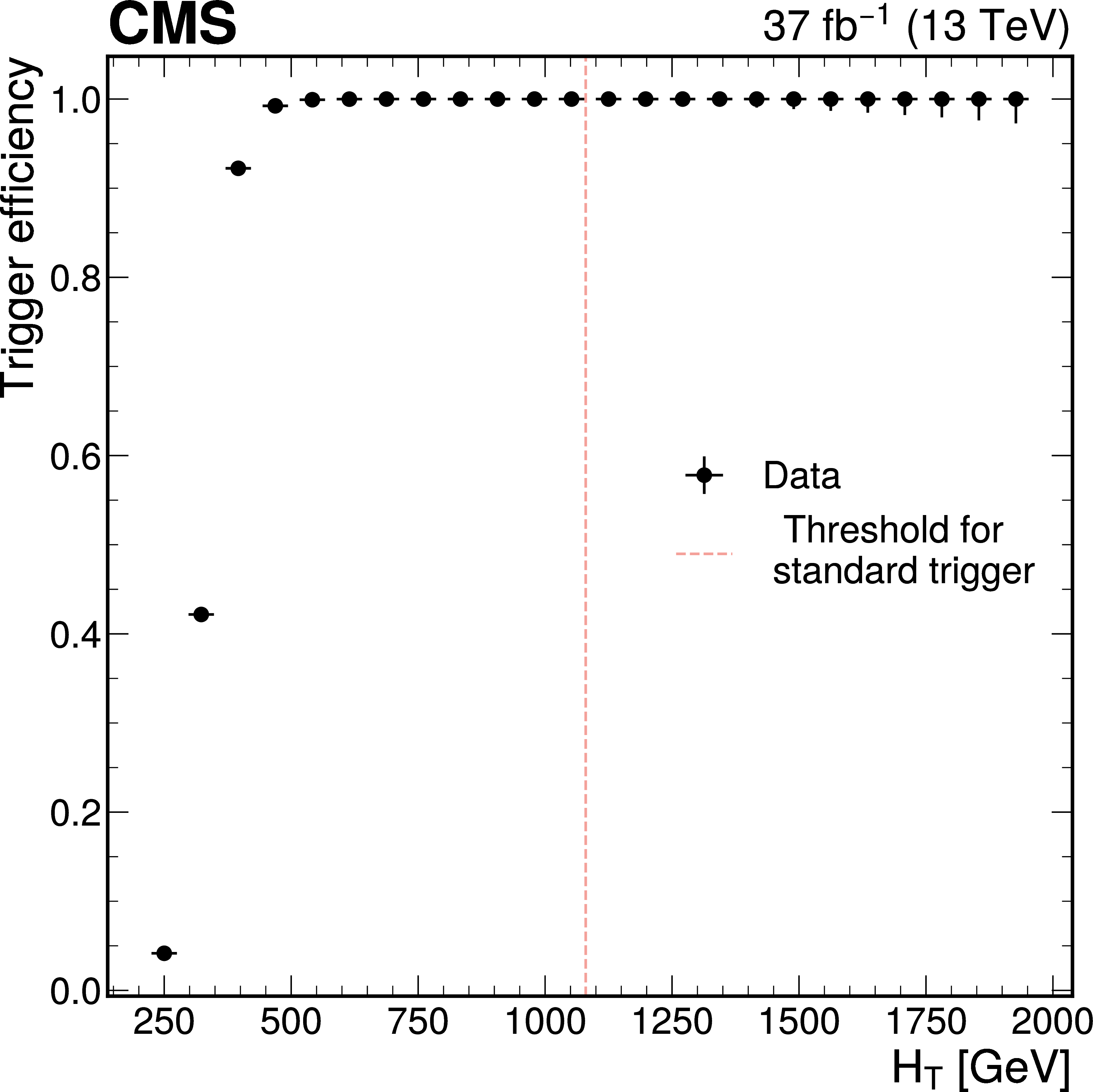
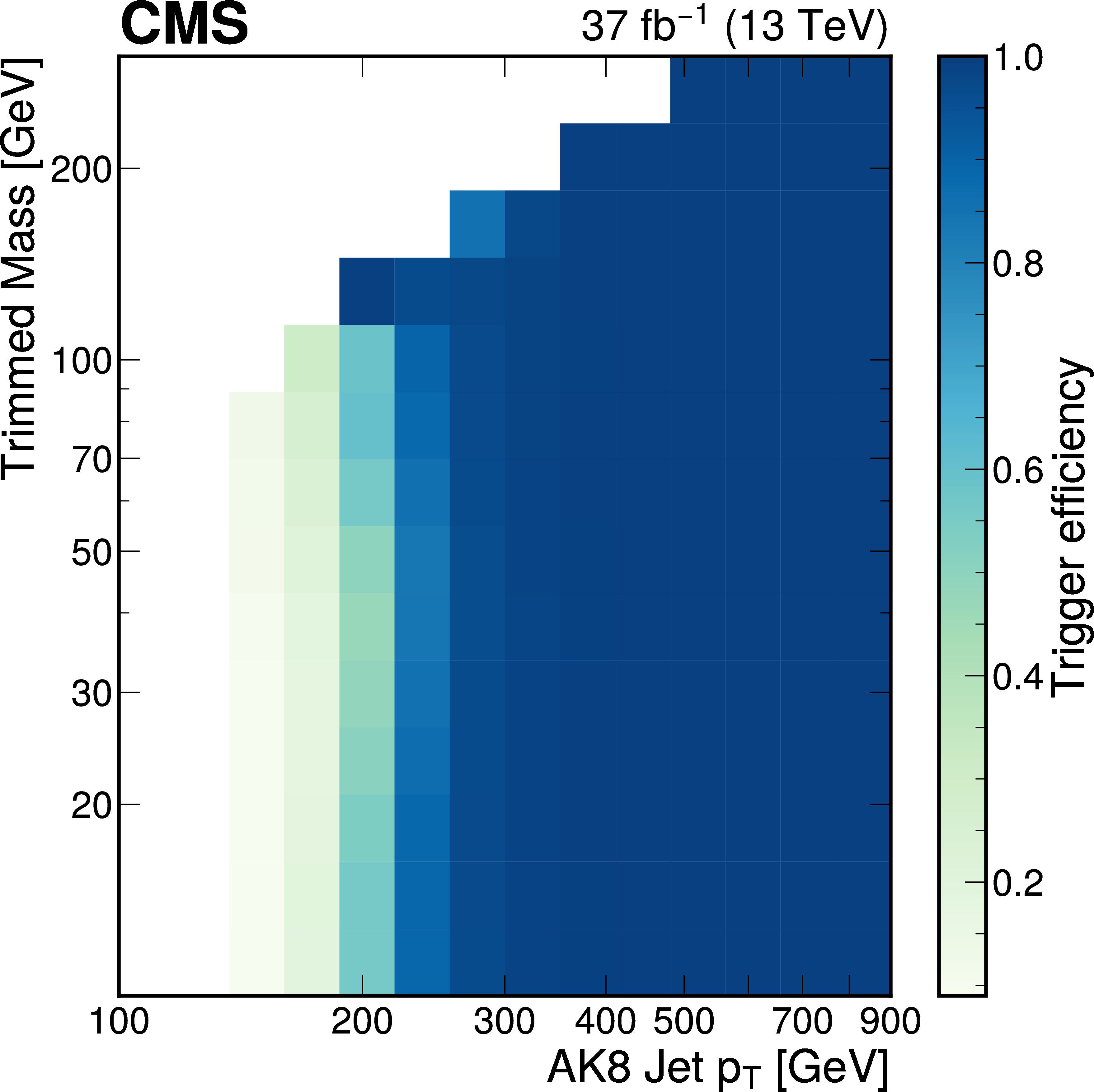
Figure 4:
The efficiency of the Run 2 PF scouting jet triggers as a function of $ H_{\mathrm{T}} $ (left) and as a function of the leading large-radius jet $ p_{\mathrm{T}} $ and trimmed jet mass (right). |
png pdf |
Figure 4-a:
The efficiency of the Run 2 PF scouting jet triggers as a function of $ H_{\mathrm{T}} $ (left) and as a function of the leading large-radius jet $ p_{\mathrm{T}} $ and trimmed jet mass (right). |
png pdf |
Figure 4-b:
The efficiency of the Run 2 PF scouting jet triggers as a function of $ H_{\mathrm{T}} $ (left) and as a function of the leading large-radius jet $ p_{\mathrm{T}} $ and trimmed jet mass (right). |

png pdf |
Figure 5:
The observed percent difference between the $ p_{\mathrm{T}} $ of Calo jets at the HLT and the $ p_{\mathrm{T}} $ of PF jets reconstructed offline (points), fitted to a smooth function (curve), vs. the Calo jet $ p_{\mathrm{T}} $. Both Calo and PF jets are calibrated with corrections derived from simulation. Figure taken from Ref. [65]. |
png pdf |
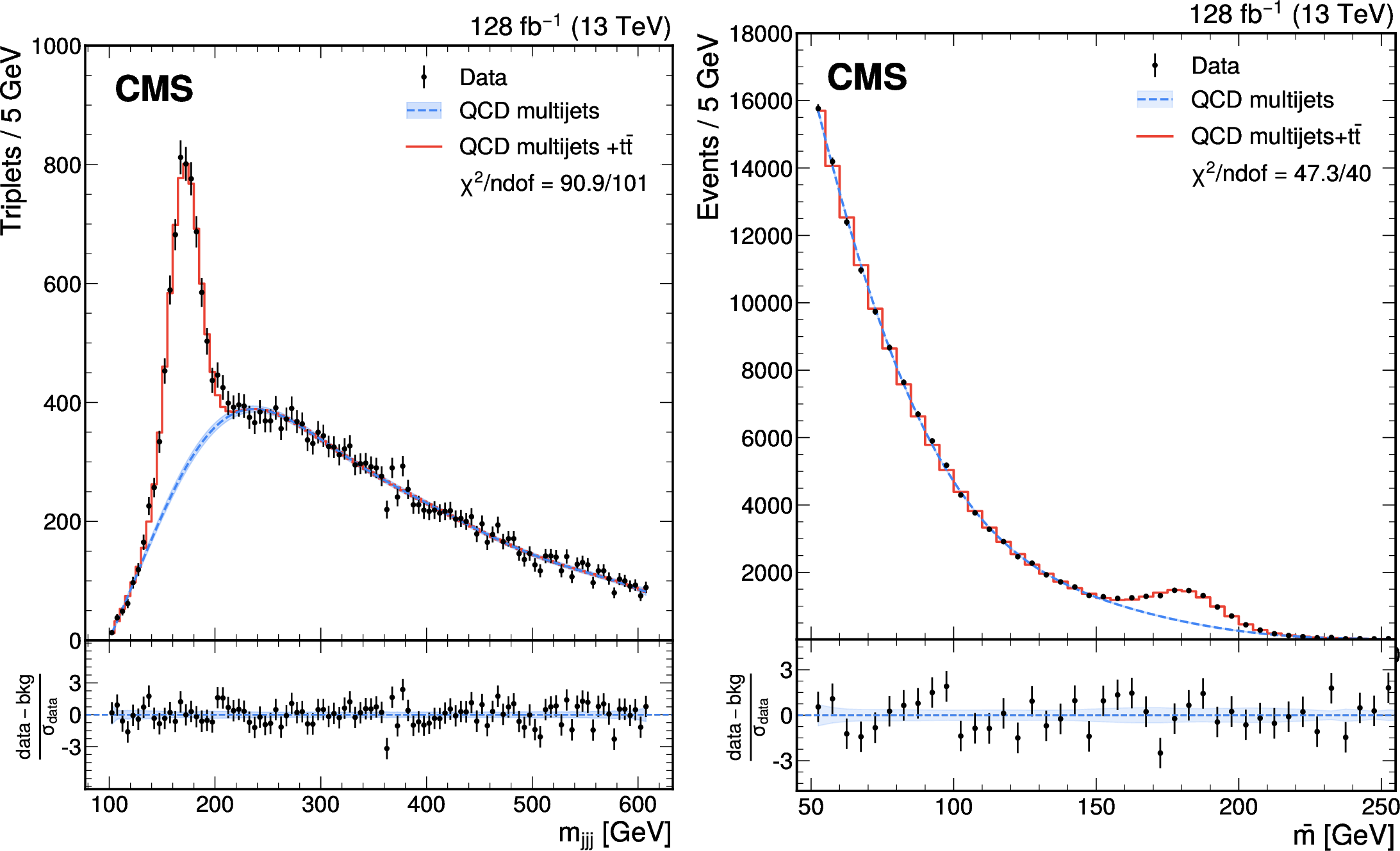
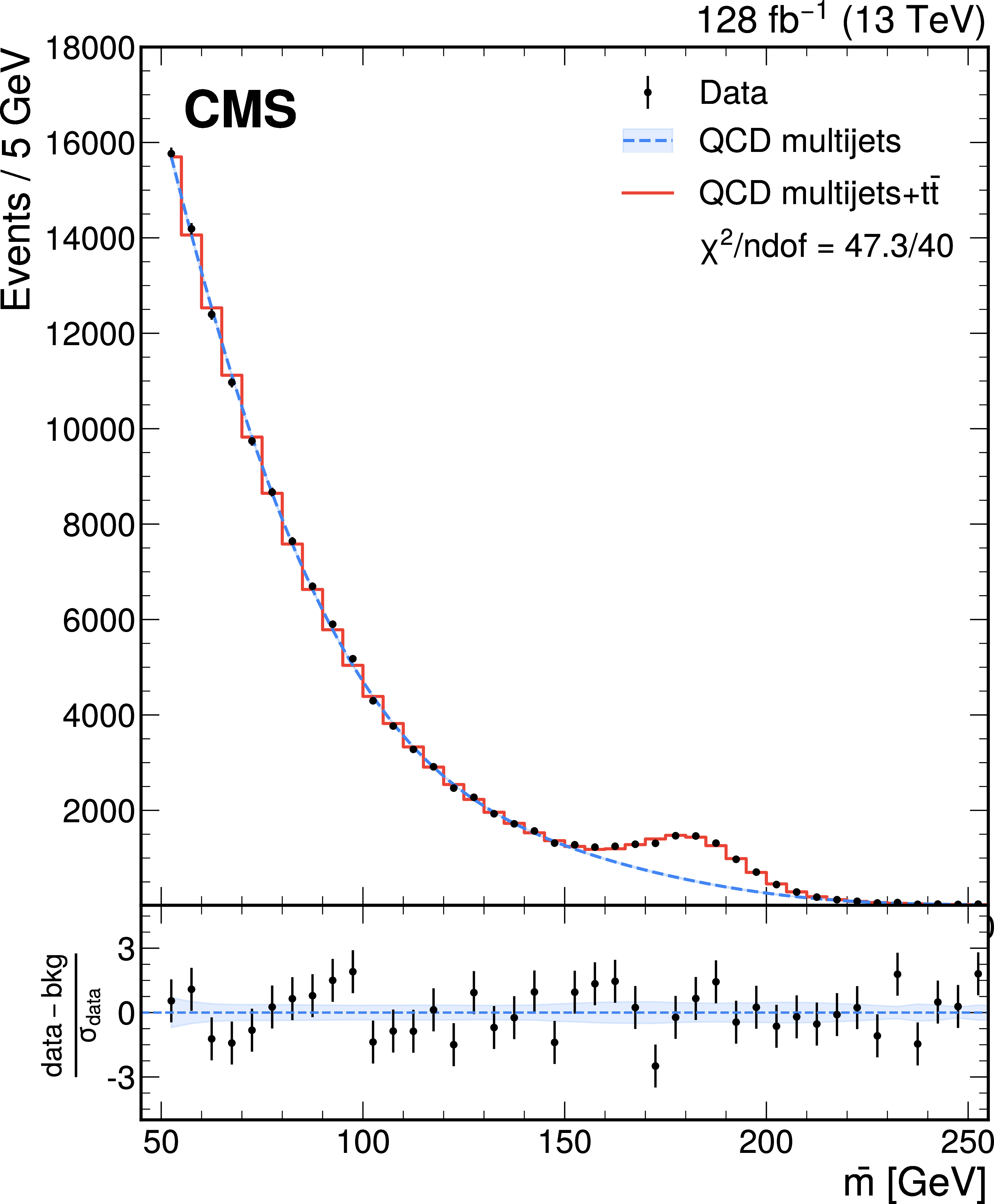
Figure 6:
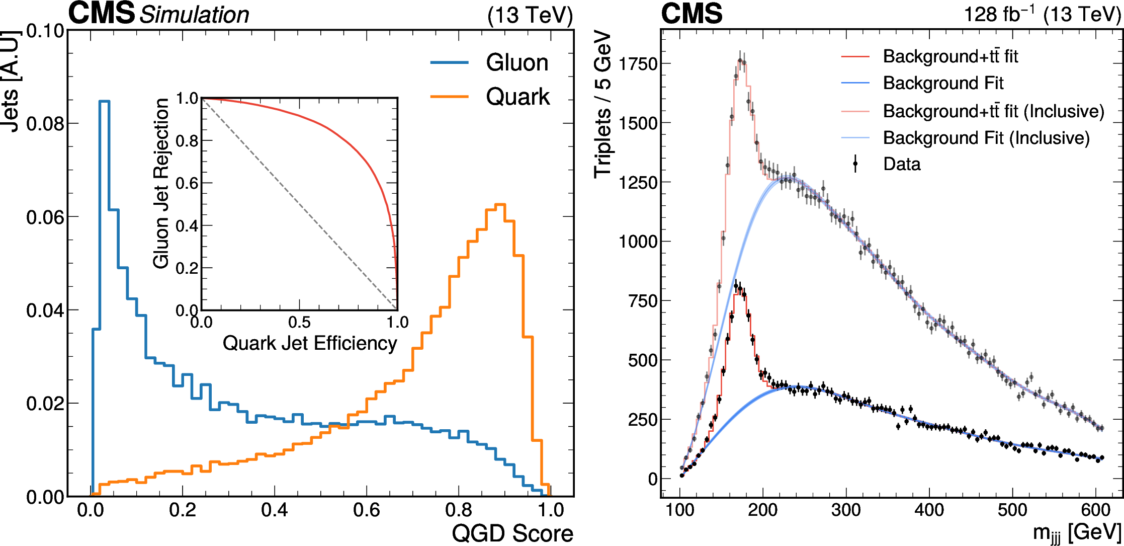
The distribution of $ m_{\mathrm{jjj}} $ for the resolved three-jet search (left), and average jet mass {($ \tilde{m} = (m_1 + m_2)/ $ 2)} for the merged three-parton search (right), adapted from Ref. [67]. Both analyses use PF jets. The peak around 170 GeV in both distributions corresponds to the all-hadronic decay of the top quark. The data (points) are compared to the background-only prediction (blue) and the full background fit including simulations of the top quark resonance (red). |

png pdf |
Figure 6-a:
The distribution of $ m_{\mathrm{jjj}} $ for the resolved three-jet search (left), and average jet mass {($ \tilde{m} = (m_1 + m_2)/ $ 2)} for the merged three-parton search (right), adapted from Ref. [67]. Both analyses use PF jets. The peak around 170 GeV in both distributions corresponds to the all-hadronic decay of the top quark. The data (points) are compared to the background-only prediction (blue) and the full background fit including simulations of the top quark resonance (red). |
png pdf |
Figure 6-b:
The distribution of $ m_{\mathrm{jjj}} $ for the resolved three-jet search (left), and average jet mass {($ \tilde{m} = (m_1 + m_2)/ $ 2)} for the merged three-parton search (right), adapted from Ref. [67]. Both analyses use PF jets. The peak around 170 GeV in both distributions corresponds to the all-hadronic decay of the top quark. The data (points) are compared to the background-only prediction (blue) and the full background fit including simulations of the top quark resonance (red). |
png pdf |
Figure 7:
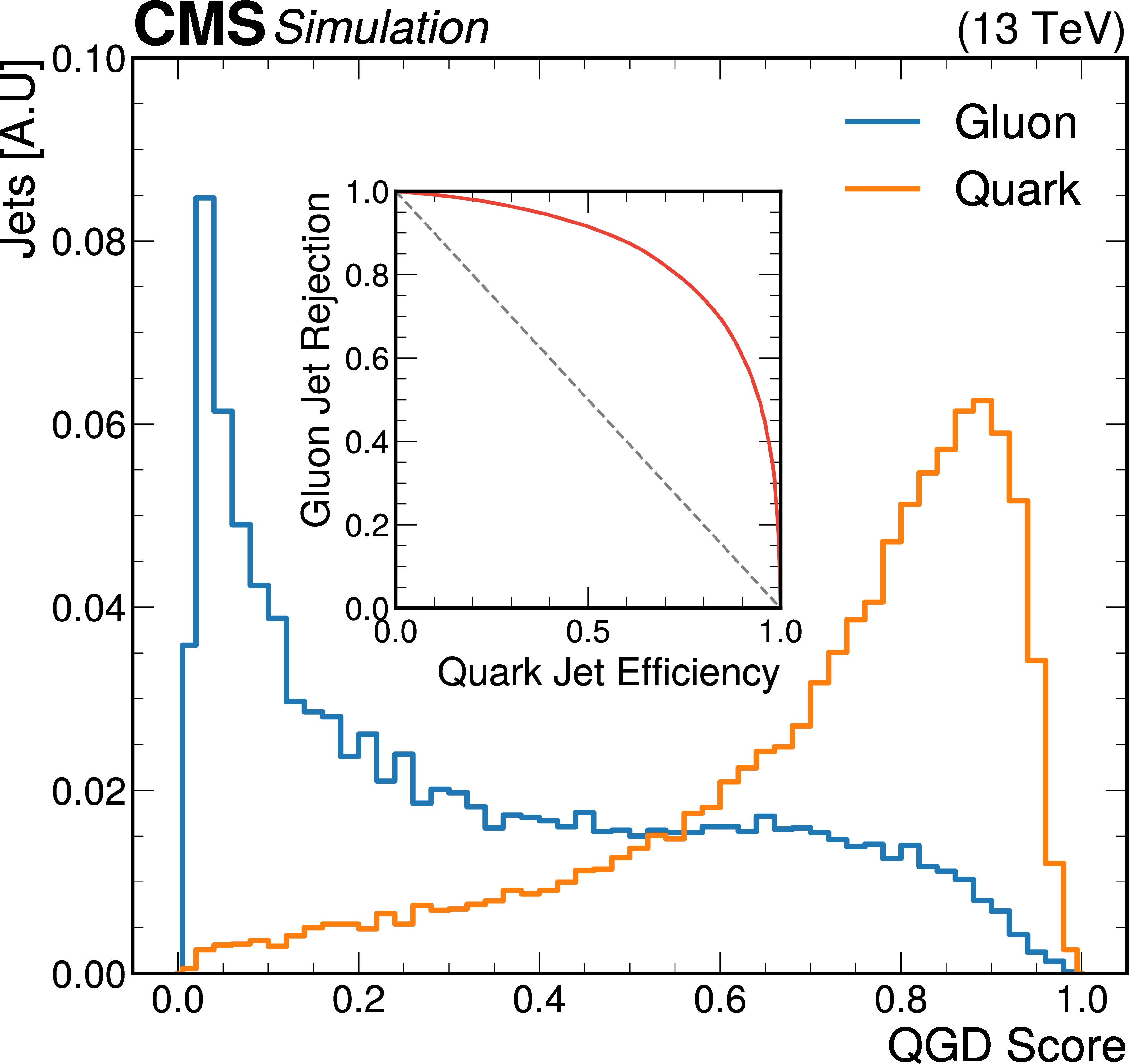
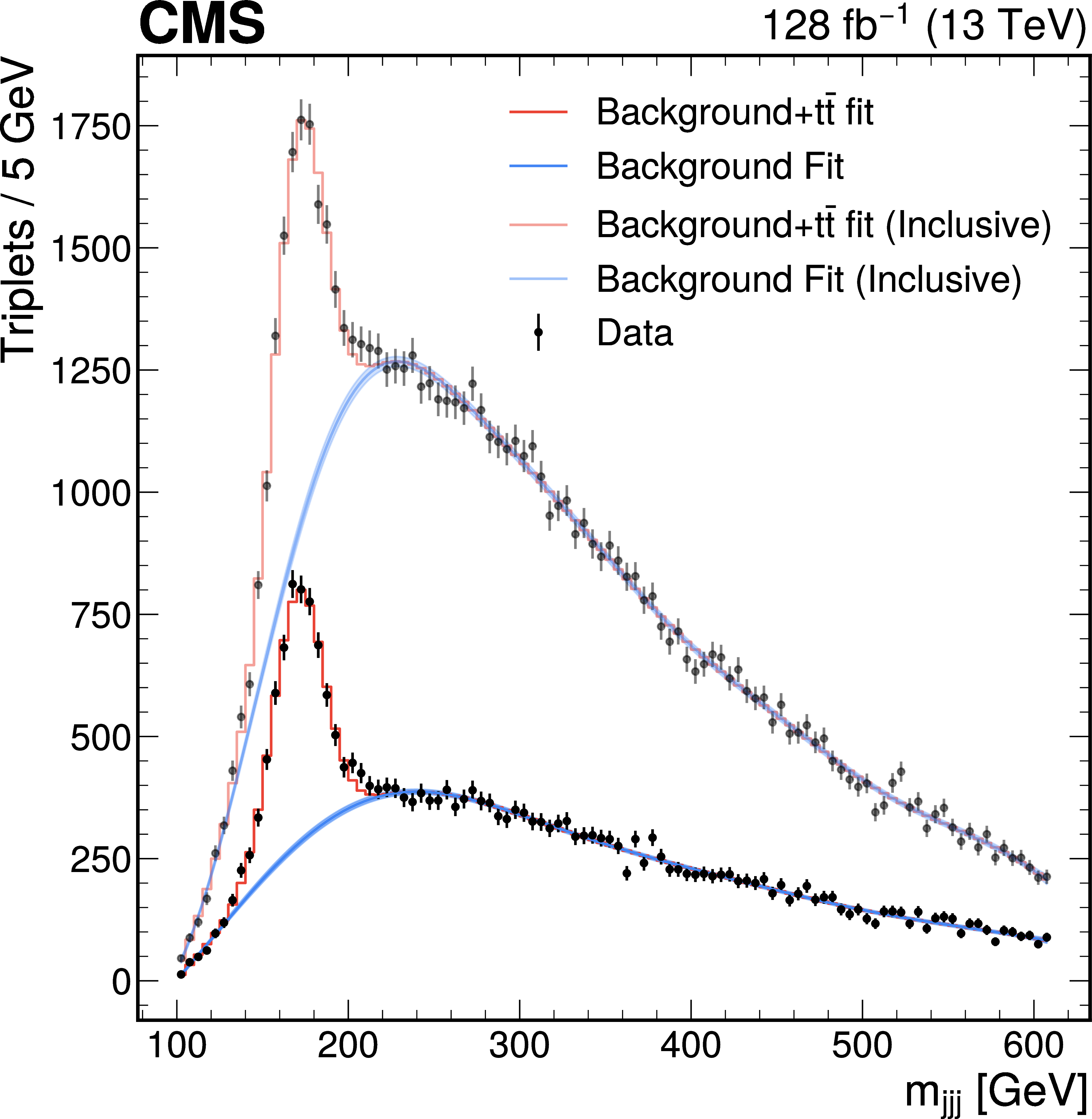
Left: output of the QGD for quark (orange) and gluon (blue) jets. The corresponding receiver operating characteristic (ROC) curve is also shown. Right: observation of fully hadronic top quark decays in the invariant mass of three jets with a QCD multijet background, for an inclusive selection (no QGD), and for a selection including the QGD score. Figure adapted from Ref. [67]. |
png pdf |
Figure 7-a:
Left: output of the QGD for quark (orange) and gluon (blue) jets. The corresponding receiver operating characteristic (ROC) curve is also shown. Right: observation of fully hadronic top quark decays in the invariant mass of three jets with a QCD multijet background, for an inclusive selection (no QGD), and for a selection including the QGD score. Figure adapted from Ref. [67]. |
png pdf |
Figure 7-b:
Left: output of the QGD for quark (orange) and gluon (blue) jets. The corresponding receiver operating characteristic (ROC) curve is also shown. Right: observation of fully hadronic top quark decays in the invariant mass of three jets with a QCD multijet background, for an inclusive selection (no QGD), and for a selection including the QGD score. Figure adapted from Ref. [67]. |

png pdf |
Figure 8:
Dimuon invariant mass distribution of events selected with the standard muon triggers (blue, dashed) and scouting muon triggers (pink, solid) in the mass range 11--240 GeV, normalized to $ {\mathcal{L}_{\text{int}}} = $ 96.6 fb$^{-1}$, corresponding to the scouting data collected in 2017 and 2018. The selection applied to obtain each distribution is described in Ref. [68]. |

png pdf |
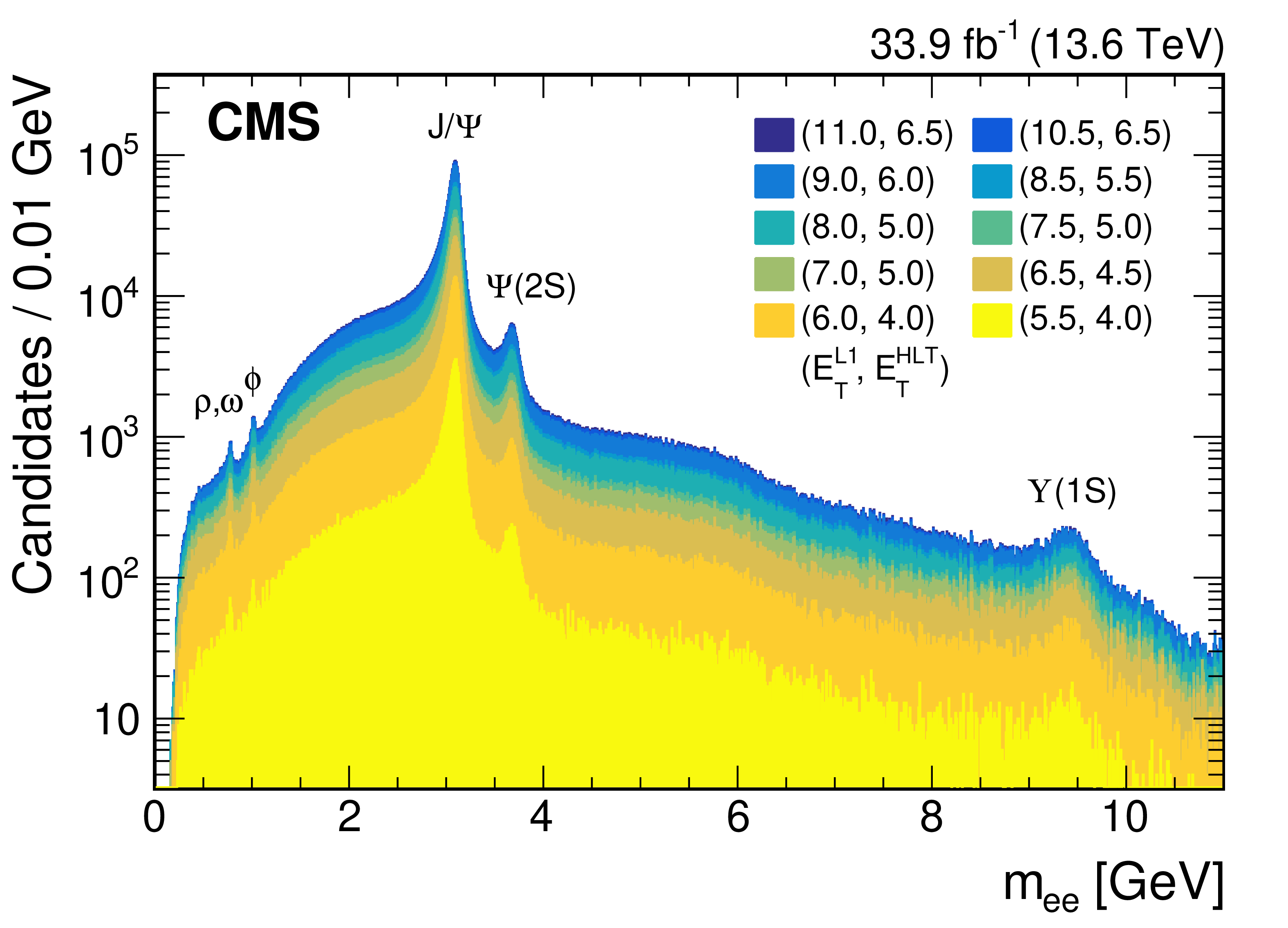
Figure 9:
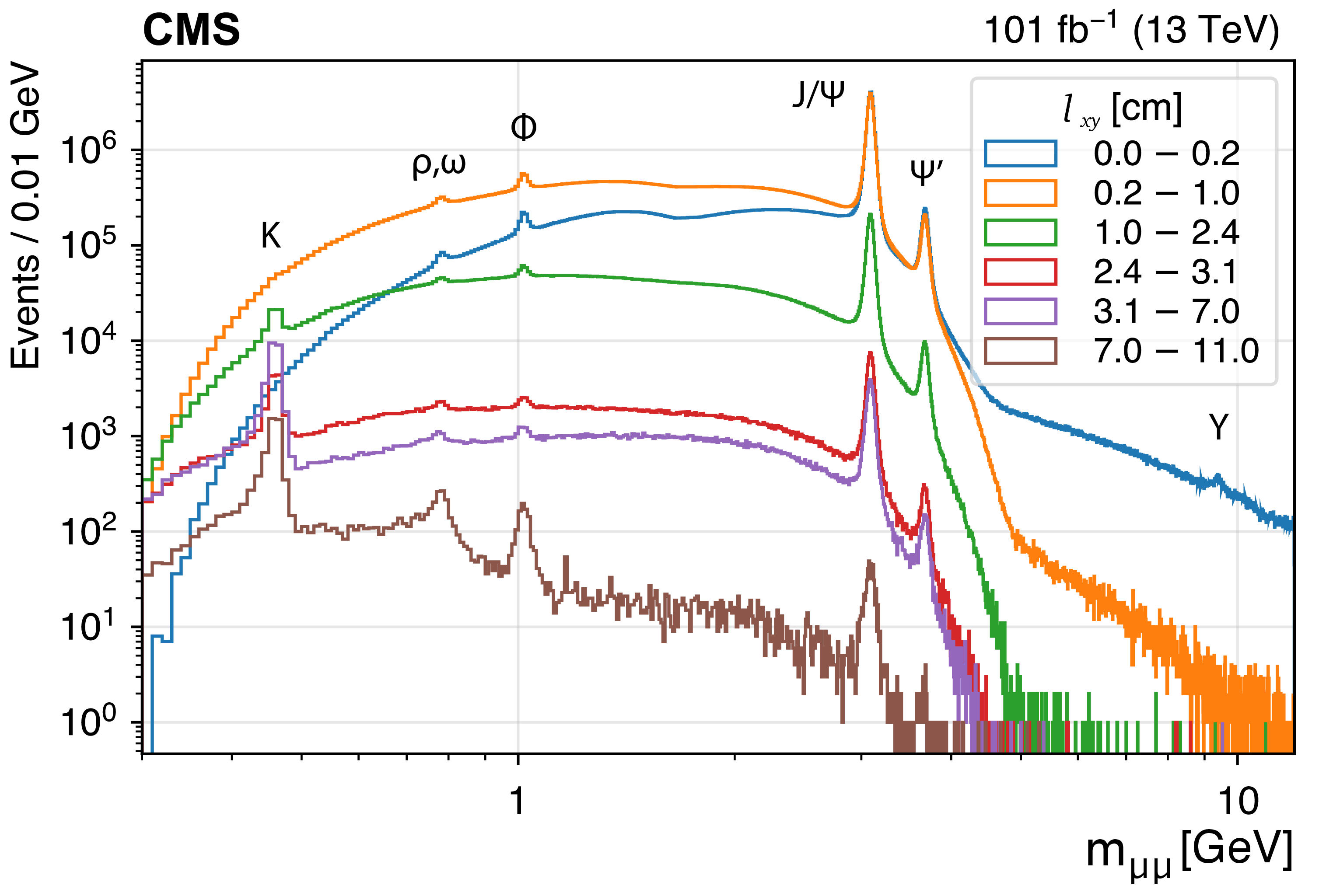
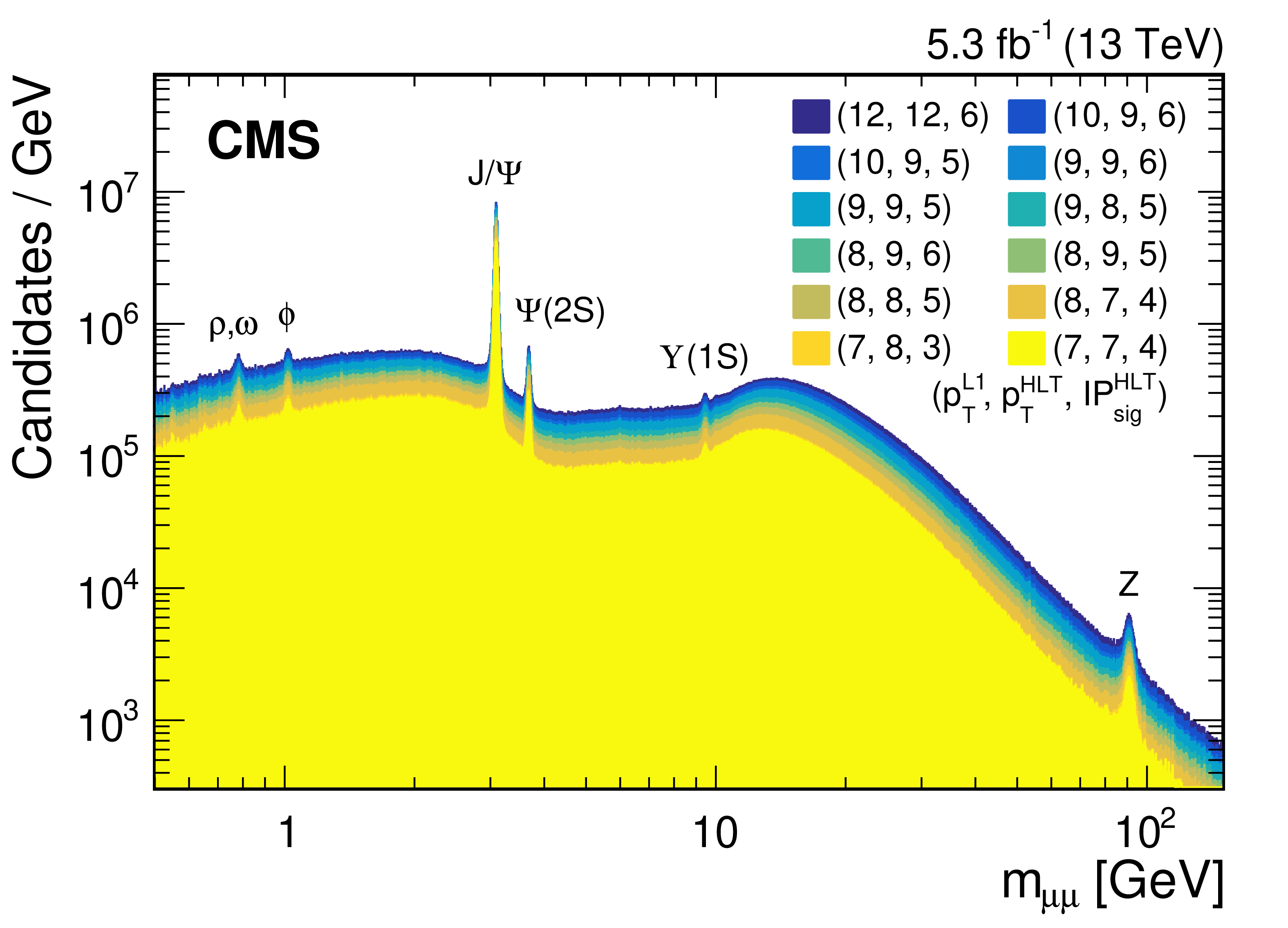
Dimuon invariant mass spectrum and event rate of each L1 seed (legend) obtained with the scouting stream reconstructed at the HLT, using data collected in 2018 corresponding to $ {\mathcal{L}_{\text{int}}} = $ 60 fb$^{-1}$. Well-known dimuon resonances from various meson decays or from Z boson decays are indicated above each peak. |
png pdf |
Figure 10:
Dimuon invariant mass distributions in bins of transverse displacement from the PV ($ l_{\text{xy}} $). Figure adapted from Ref. [69]. |
png pdf |
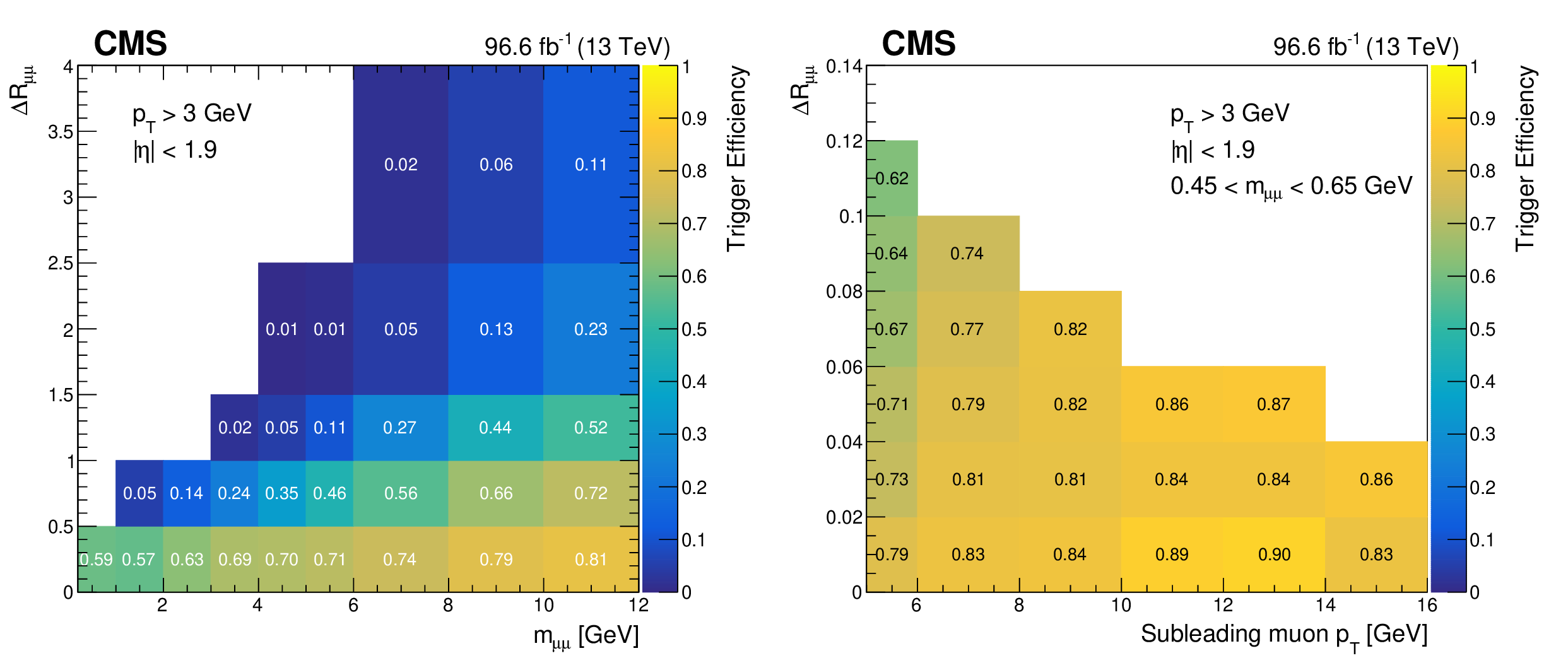
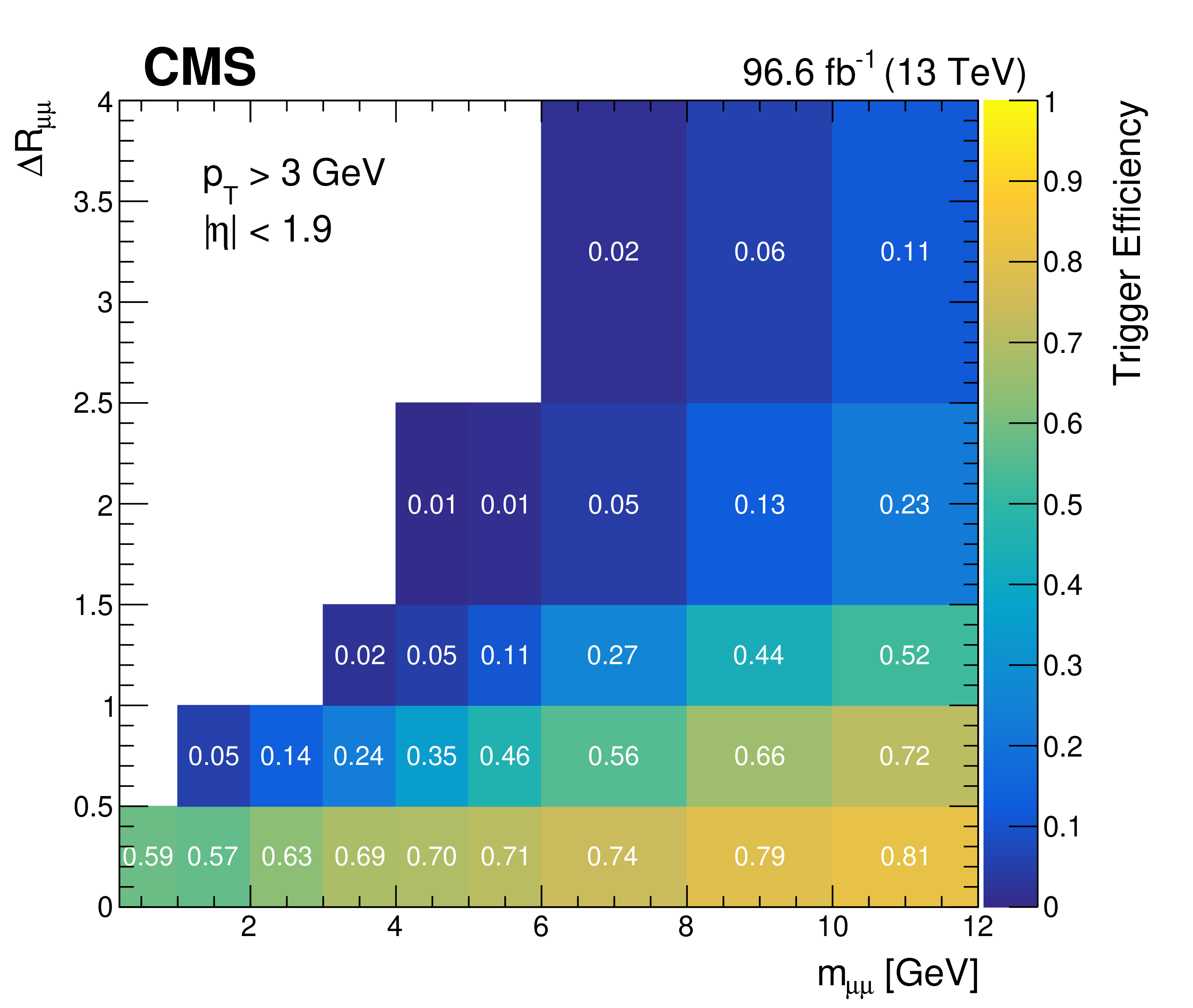
Figure 11:
Efficiency of the dimuon scouting trigger and logical ``OR'' of all L1 triggers measured with 2017 and 2018 data. The efficiency is shown as a function of the angular separation between the two muons $ {\Delta}R_{\mu\mu} $ and the dimuon mass $ m_{\mu\mu} $ (left), and as a function of $ {\Delta}R_{\mu\mu} $ and the subleading muon $ p_{\mathrm{T}} $ (right). The selection in the right plot also requires 0.45 $ < m_{\mu\mu} < $ 0.65 GeV to focus on the $ \eta $ meson resonance region. The statistical uncertainty in the measured values is generally less than 3% per bin on the left plot and less than 15% per bin on the right plot. |
png pdf |
Figure 11-a:
Efficiency of the dimuon scouting trigger and logical ``OR'' of all L1 triggers measured with 2017 and 2018 data. The efficiency is shown as a function of the angular separation between the two muons $ {\Delta}R_{\mu\mu} $ and the dimuon mass $ m_{\mu\mu} $ (left), and as a function of $ {\Delta}R_{\mu\mu} $ and the subleading muon $ p_{\mathrm{T}} $ (right). The selection in the right plot also requires 0.45 $ < m_{\mu\mu} < $ 0.65 GeV to focus on the $ \eta $ meson resonance region. The statistical uncertainty in the measured values is generally less than 3% per bin on the left plot and less than 15% per bin on the right plot. |

png pdf |
Figure 11-b:
Efficiency of the dimuon scouting trigger and logical ``OR'' of all L1 triggers measured with 2017 and 2018 data. The efficiency is shown as a function of the angular separation between the two muons $ {\Delta}R_{\mu\mu} $ and the dimuon mass $ m_{\mu\mu} $ (left), and as a function of $ {\Delta}R_{\mu\mu} $ and the subleading muon $ p_{\mathrm{T}} $ (right). The selection in the right plot also requires 0.45 $ < m_{\mu\mu} < $ 0.65 GeV to focus on the $ \eta $ meson resonance region. The statistical uncertainty in the measured values is generally less than 3% per bin on the left plot and less than 15% per bin on the right plot. |
png pdf |
Figure 12:
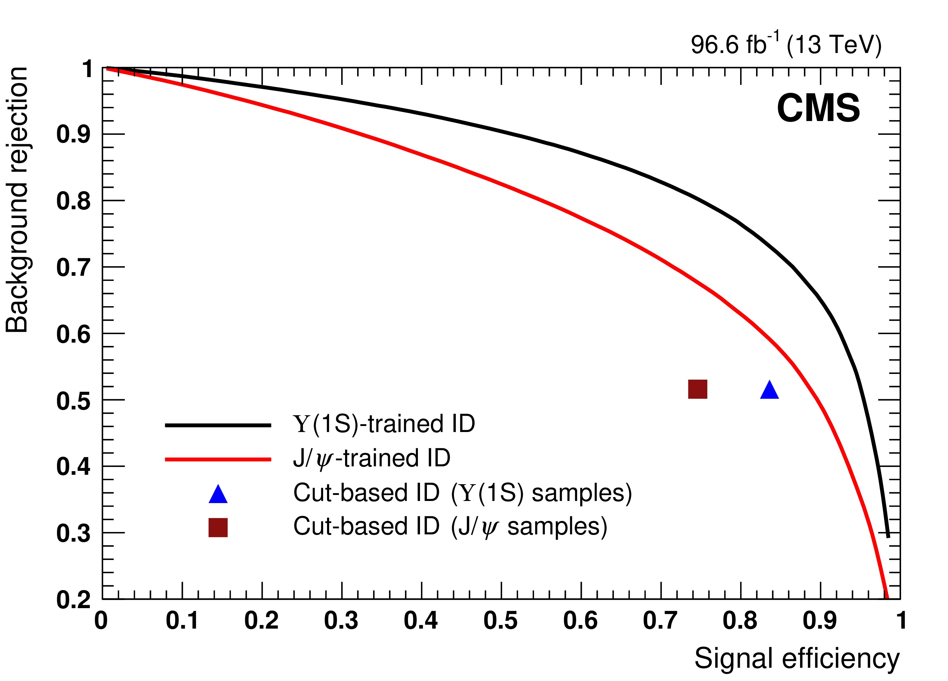
Background rejection vs. signal efficiency of the new MVA-based muon ID strategies evaluated on scouting data: $ \Upsilon{\textrm{(1S)}} $-trained MVA (black line), $ \mathrm{J}/\psi $-trained MVA (red line). A comparison with the performance of the previous cut-based selection, which was optimised for signals at the mass range higher than 11 GeV, is also shown for the $ \Upsilon{\textrm{(1S)}} $ (blue triangle) and $ \mathrm{J}/\psi $ (brown square) signals. Figure adapted from Ref. [71]. |
png pdf |
Figure 13:
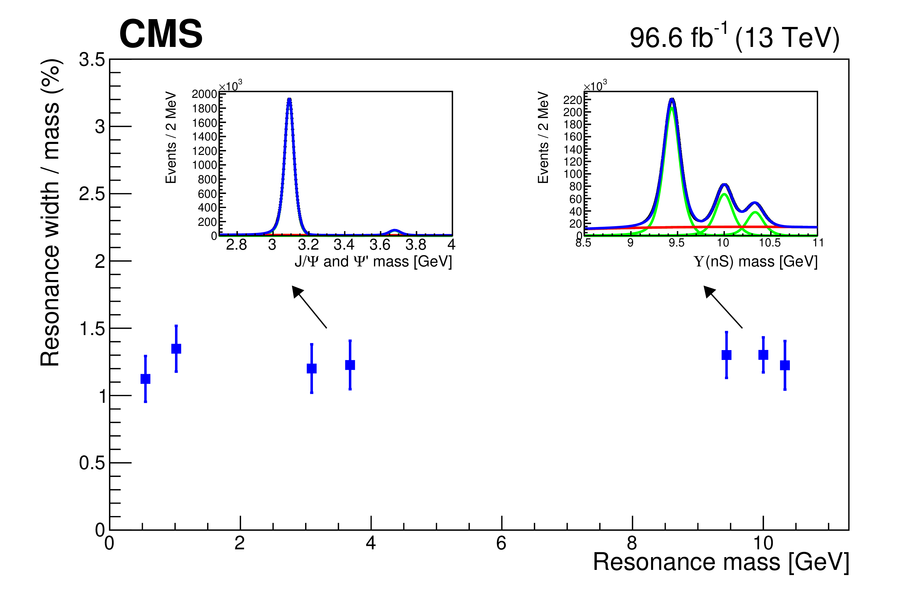
Relative width of dimuon resonances as a function of mass, measured in 2017 and 2018 scouting data. The fits are performed separately for the 2017 and 2018 data sets. The values shown are the average width of each fit, weighted by the $ \mathcal{L}_{\text{int}} $ value corresponding to the data accumulated in each year. From left to right, the $ \eta $, $ \phi $, $ \mathrm{J}/\psi $, \PGyP2S, $ \Upsilon{\textrm{(1S)}} $, $ \Upsilon{\textrm{(2S)}} $, and $ \Upsilon{\textrm{(3S)}} $ resonances are shown. The inserts display fits of the $ \mathrm{J}/\psi $ and $ \Upsilon $ peaks obtained with scouting data (black markers) separately for the signal (green) and background (red) components, and for their sum (blue). |

png pdf |
Figure 14:
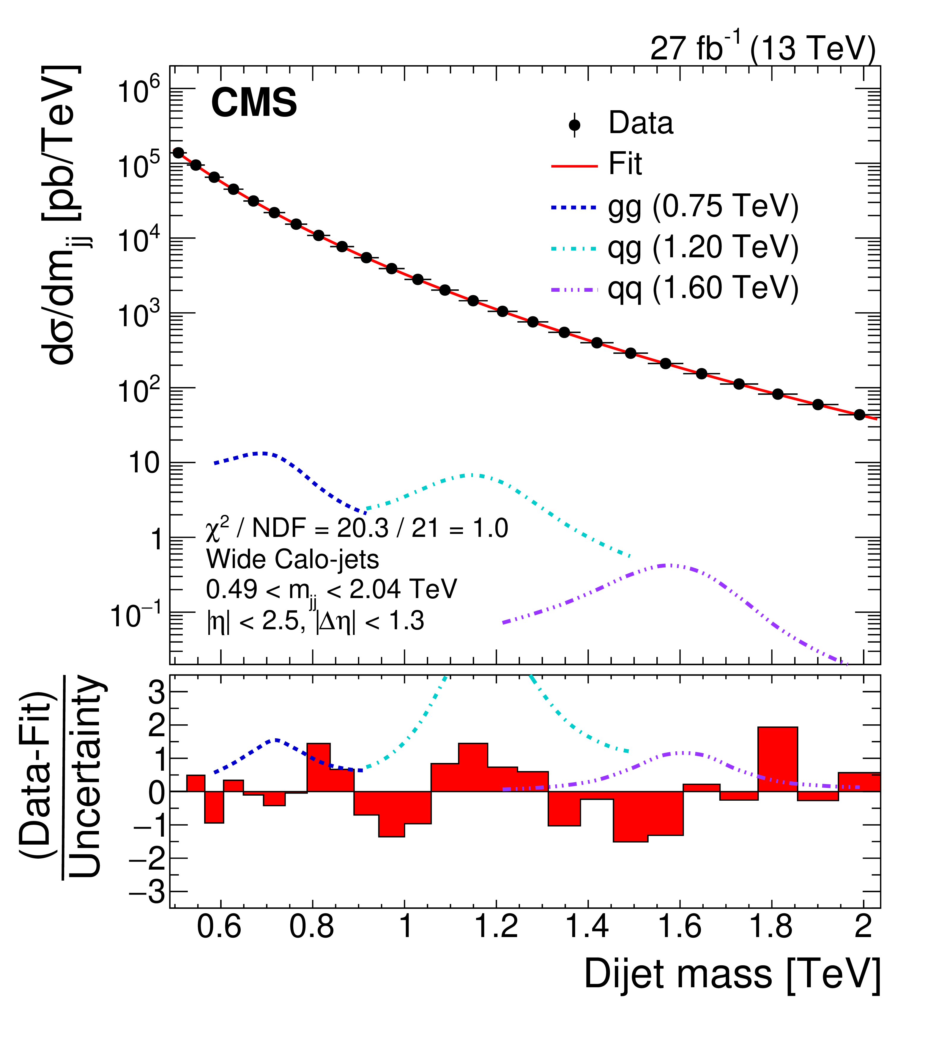
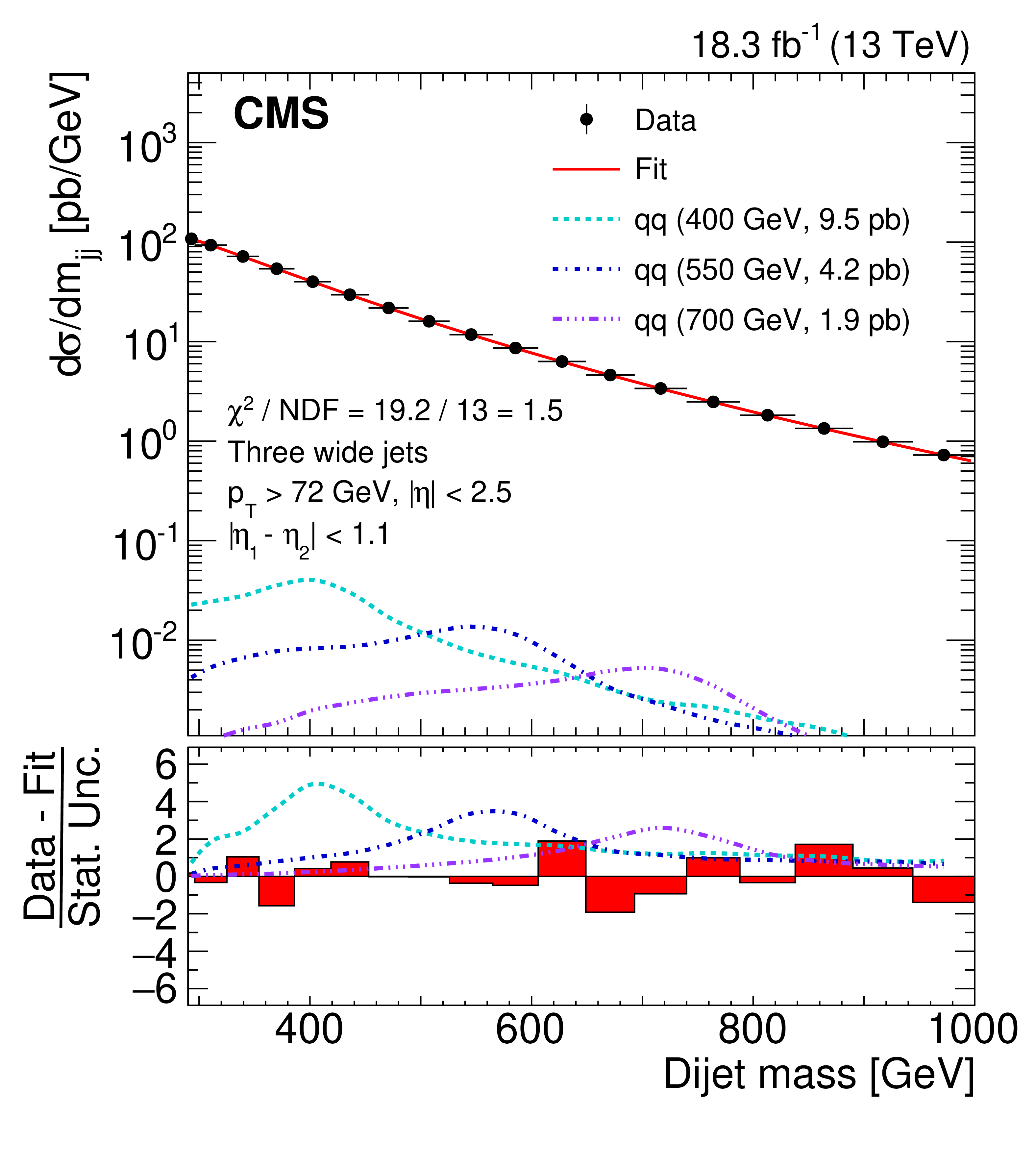
Left: dijet mass spectra (points) compared to a fitted parametrization of the background (solid curve) for the inclusive search performed in Ref. [65]. Right: dijet mass spectrum (points) compared to a fitted parametrization of the background (solid curve) for the three-jet analysis performed in Ref. [77]. The lower panel shows the difference between the data and the fitted parametrization, divided by the statistical uncertainty of the data. Examples of predicted signals from narrow gluon-gluon, quark-gluon, and quark-quark resonances are shown with cross sections equal to the observed upper limits at 95% CL. Figures taken from Refs. [65] (left) and [77] (right). |
png pdf |
Figure 14-a:
Left: dijet mass spectra (points) compared to a fitted parametrization of the background (solid curve) for the inclusive search performed in Ref. [65]. Right: dijet mass spectrum (points) compared to a fitted parametrization of the background (solid curve) for the three-jet analysis performed in Ref. [77]. The lower panel shows the difference between the data and the fitted parametrization, divided by the statistical uncertainty of the data. Examples of predicted signals from narrow gluon-gluon, quark-gluon, and quark-quark resonances are shown with cross sections equal to the observed upper limits at 95% CL. Figures taken from Refs. [65] (left) and [77] (right). |
png pdf |
Figure 14-b:
Left: dijet mass spectra (points) compared to a fitted parametrization of the background (solid curve) for the inclusive search performed in Ref. [65]. Right: dijet mass spectrum (points) compared to a fitted parametrization of the background (solid curve) for the three-jet analysis performed in Ref. [77]. The lower panel shows the difference between the data and the fitted parametrization, divided by the statistical uncertainty of the data. Examples of predicted signals from narrow gluon-gluon, quark-gluon, and quark-quark resonances are shown with cross sections equal to the observed upper limits at 95% CL. Figures taken from Refs. [65] (left) and [77] (right). |
png pdf |
Figure 15:
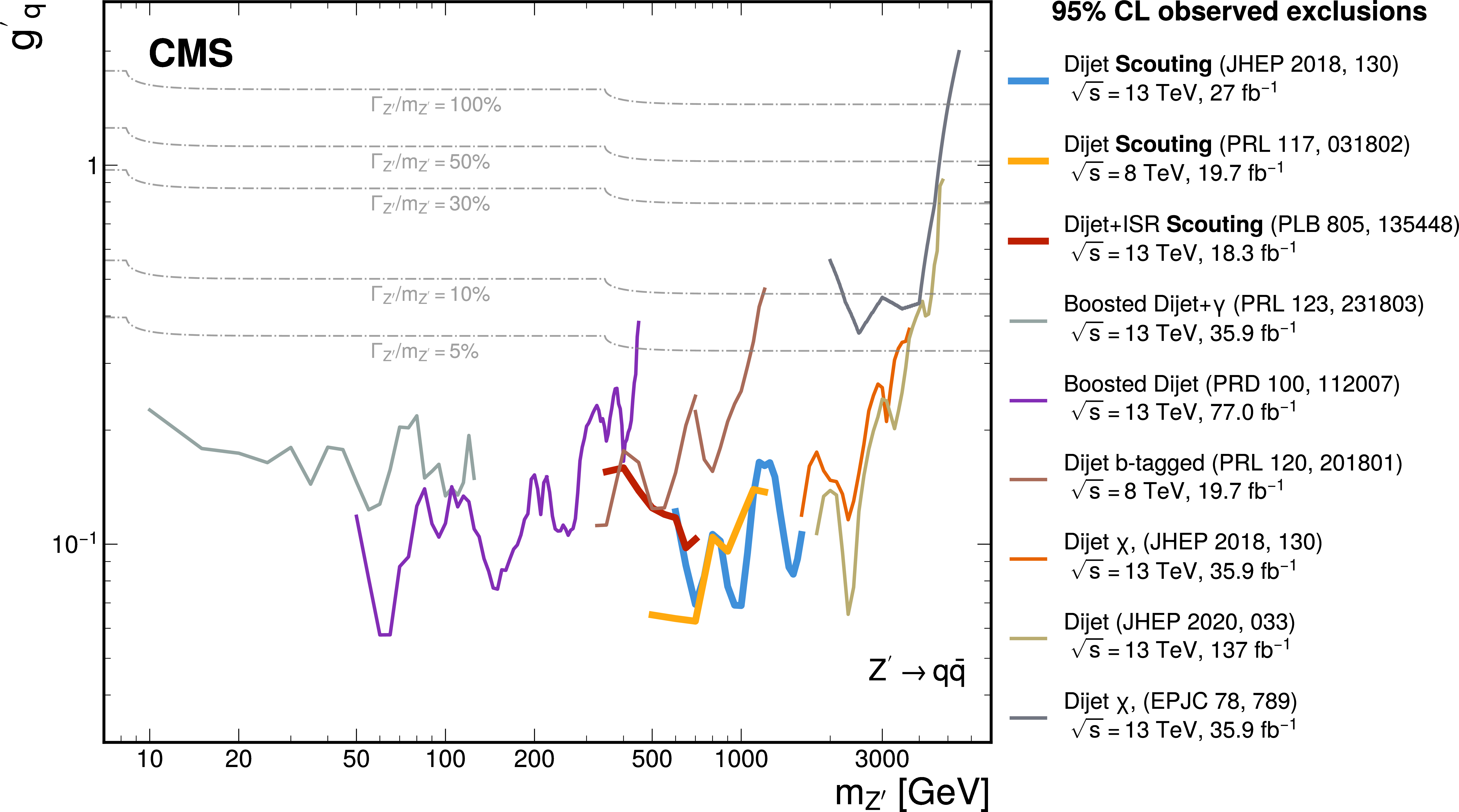
Observed limits on the universal coupling $ g^\prime_\mathrm{q} $ between a leptophobic $ \mathrm{Z}^{'} $ boson and quarks [76] from various CMS dijet analyses. Regions above the lines are excluded at 95% CL. The grey dashed lines show the $ g^\prime_\mathrm{q} $ values at fixed values of $ {\Gamma_{\mathrm{Z}^{'}}/m_{\mathrm{Z}^{'}}} $. Limits from scouting-based analyses are indicated with bold lines. |

png pdf |
Figure 16:
Comparison of limits from searches for RPV gluinos decaying to three partons. Regions above the lines are excluded at 95% CL. The two CMS analyses that use data scouting are also indicated with bold lines. |
png pdf |
Figure 17:
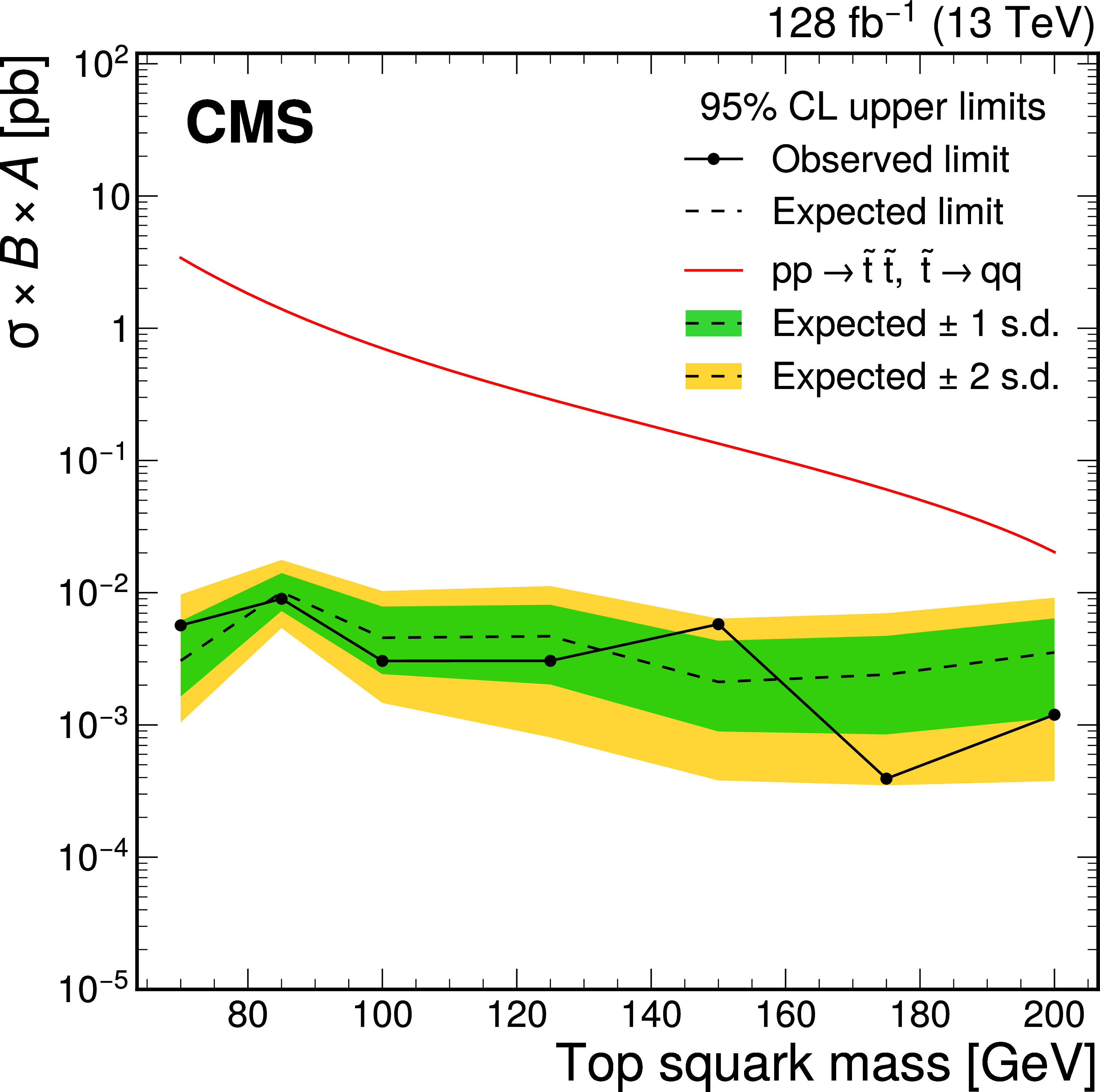
Observed (points) and expected (dashes) limits on the product of production cross section, branching fraction, and acceptance for pair-produced merged two-quark resonances. The variations at the one and two standard deviation levels in the expected limits are displayed with shaded bands. A comparison with the theoretical predictions for top squark production (red) is also shown. Figure taken from Ref. [67]. |

png pdf |
Figure 18:
Expected and observed upper limits at 90% CL on the square of the kinetic mixing coefficient ($ \epsilon^2 $) as a function of dark photon mass. Results obtained with scouting triggers are displayed to the left of the vertical purple line, while those obtained with standard triggers are shown to the right. Limits at 90% CL obtained from the search performed by the LHCb Collaboration [90] are shown in red, and constraints at 95% CL from the measurements of electroweak observables are shown in light blue [91]. Figure taken from Ref. [68]. |
png pdf |
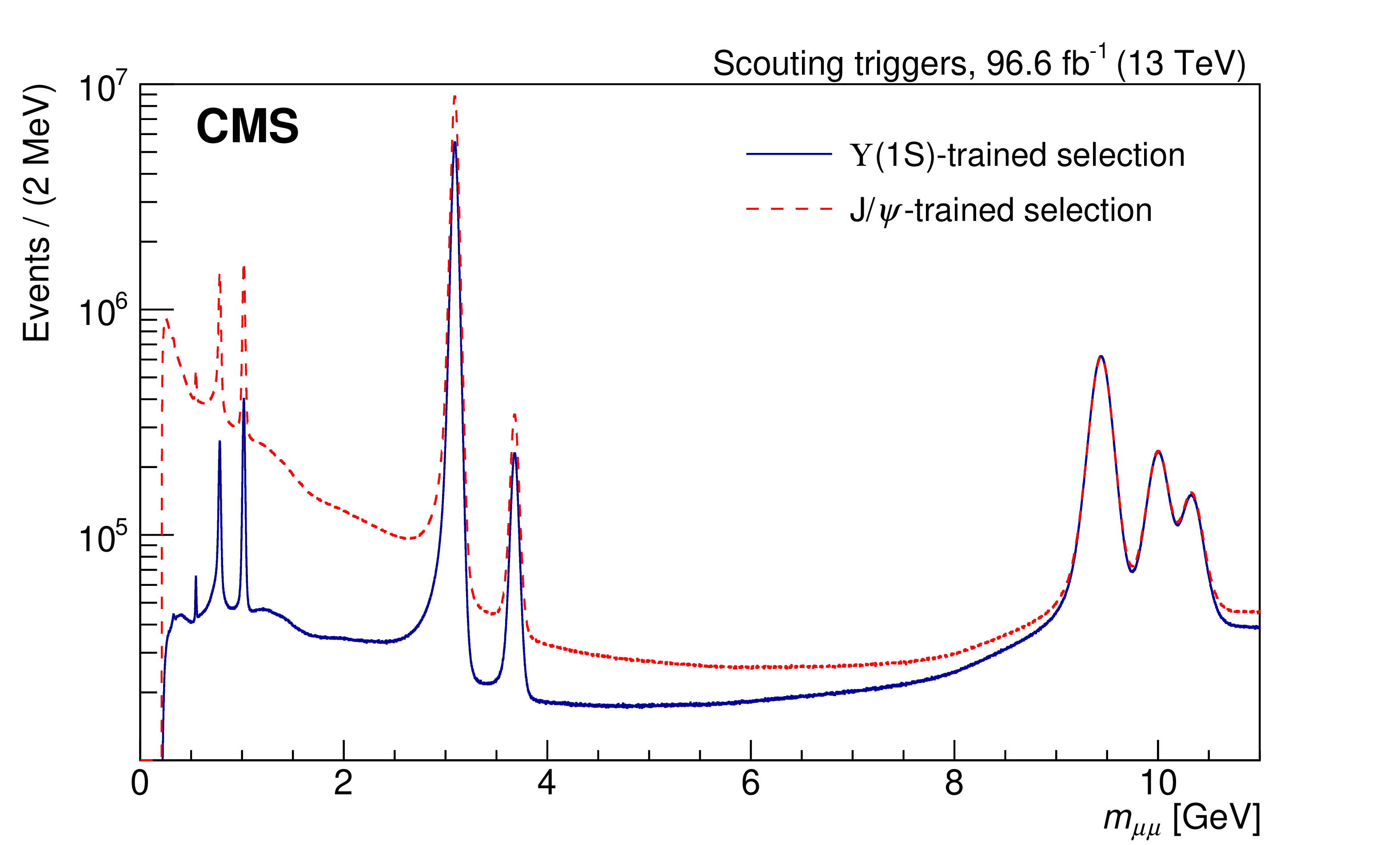
Figure 19:
The $ m_{\mu\mu} $ distribution obtained with the scouting data collected during 2017 and 2018 with two sets of selections: the $ \mathrm{J}/\psi $-trained (red) and the $ \Upsilon{\textrm{(1S)}} $-trained (blue) MVA-based muon identification algorithms. Figure taken from Ref. [71]. |
png pdf |
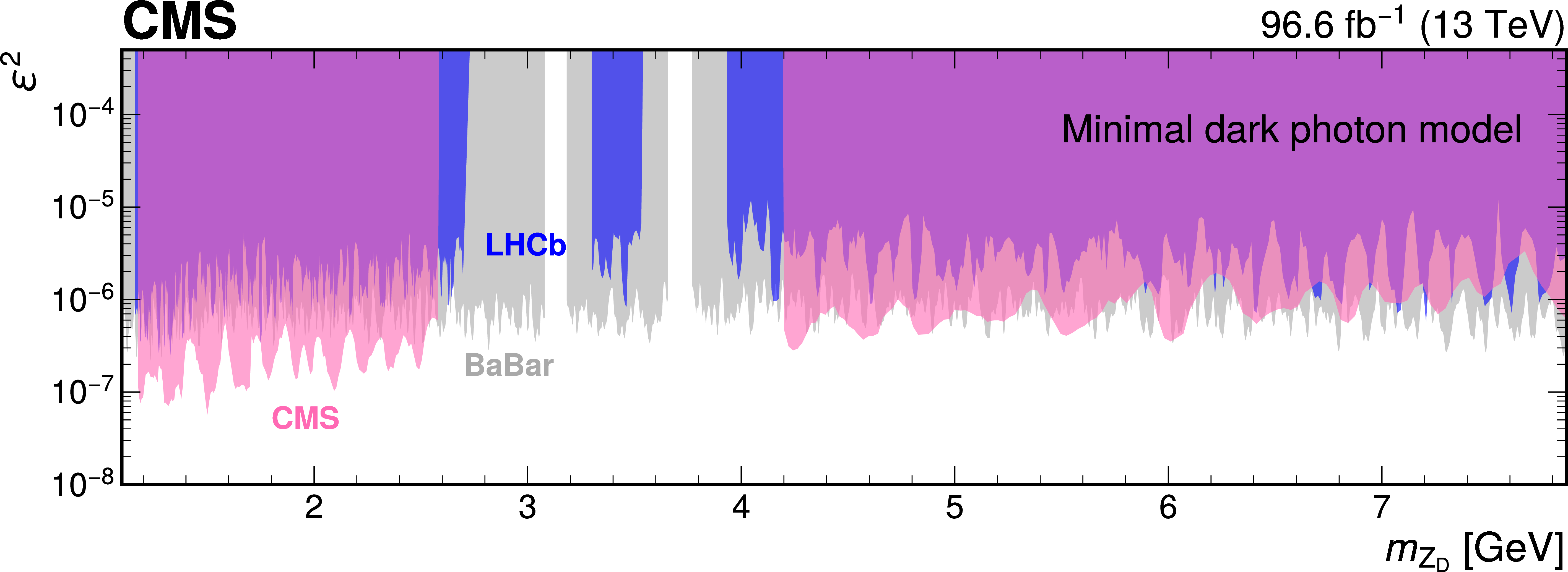
Figure 20:
Upper limits at 90% CL on the square of the kinetic mixing coefficient ($ \epsilon^2 $) in the minimal dark photon model obtained as a recast of model-independent limits on the production rates of dimuon resonances for the inclusive category. The CMS limits (pink) are compared with the existing limits at 90% CL provided by LHCb [92] (blue) and BaBar [93] (gray). Figure taken from Ref. [71]. |
png pdf |
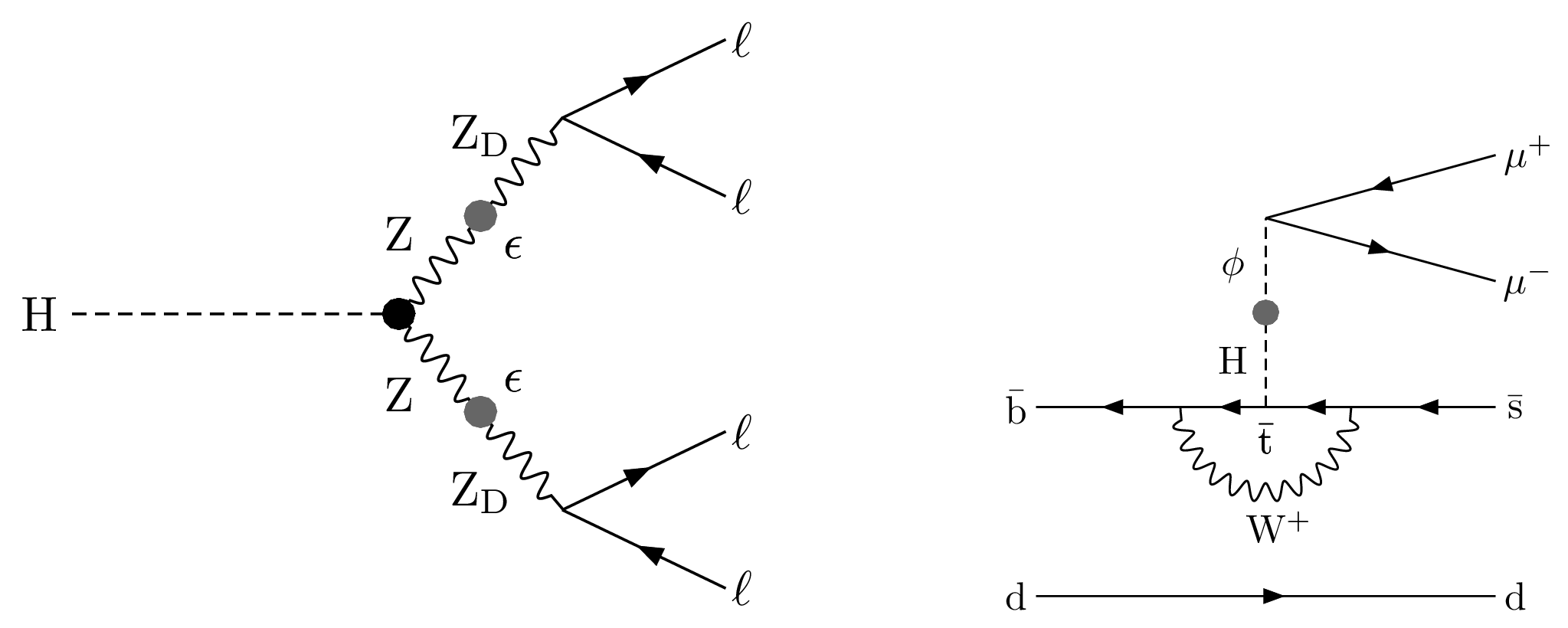
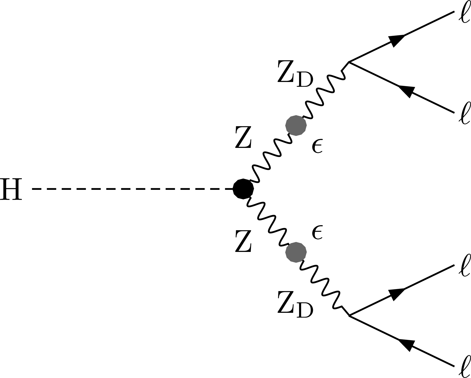
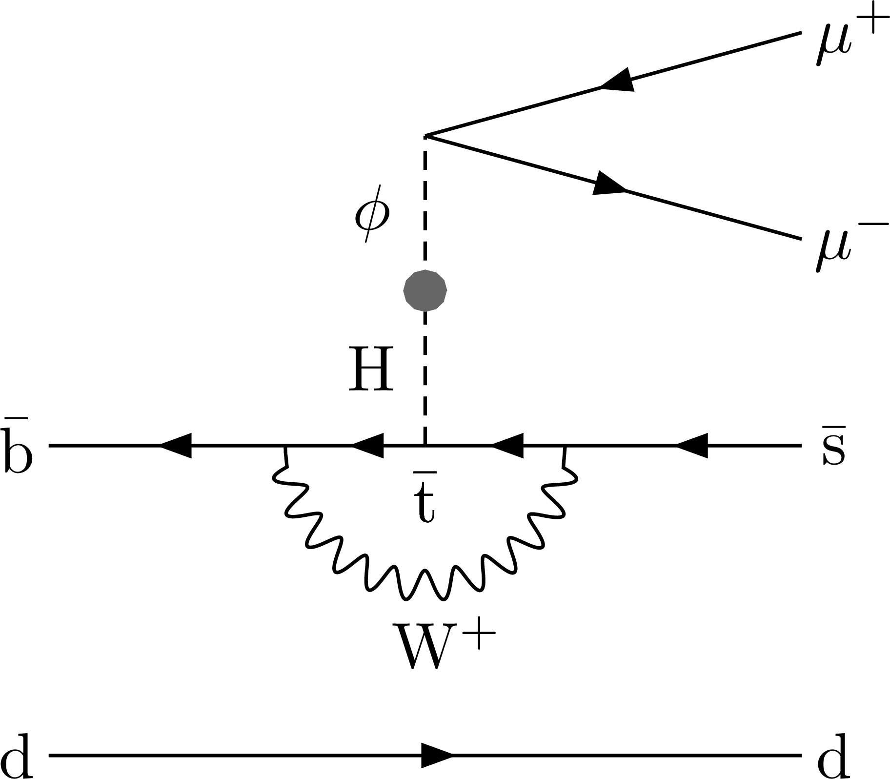
Figure 21:
Left: diagram illustrating an SM-like Higgs boson (H) decay to four leptons ($ \ell $) via two intermediate dark photons ($\mathrm{Z_D}$). Right: diagram illustrating the production of a scalar resonance $ \phi $ in a b hadron decay, through mixing with an SM-like Higgs boson. Figure taken from Ref. [69]. |
png pdf |
Figure 21-a:
Left: diagram illustrating an SM-like Higgs boson (H) decay to four leptons ($ \ell $) via two intermediate dark photons ($\mathrm{Z_D}$). Right: diagram illustrating the production of a scalar resonance $ \phi $ in a b hadron decay, through mixing with an SM-like Higgs boson. Figure taken from Ref. [69]. |
png pdf |
Figure 21-b:
Left: diagram illustrating an SM-like Higgs boson (H) decay to four leptons ($ \ell $) via two intermediate dark photons ($\mathrm{Z_D}$). Right: diagram illustrating the production of a scalar resonance $ \phi $ in a b hadron decay, through mixing with an SM-like Higgs boson. Figure taken from Ref. [69]. |
png pdf |
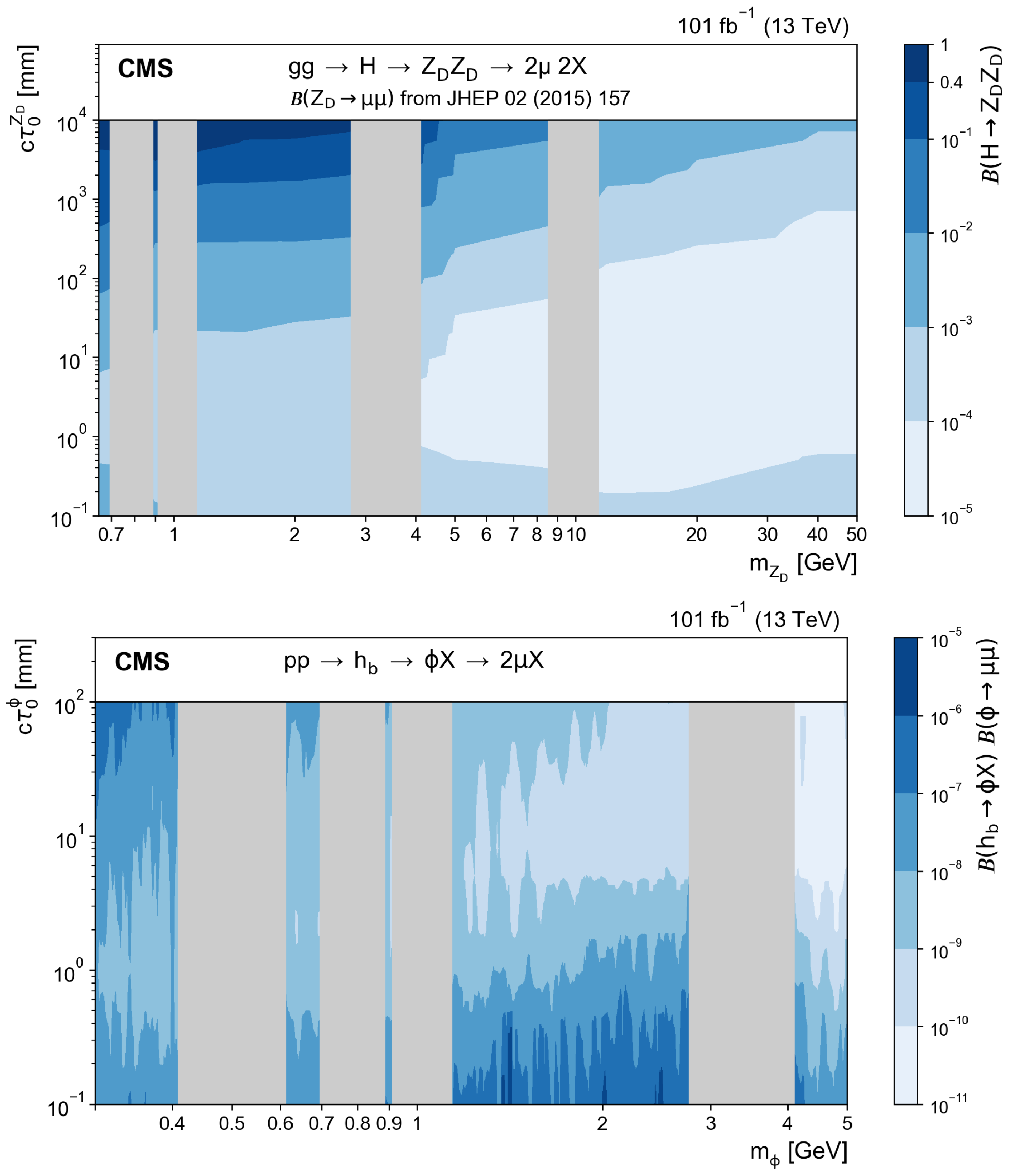
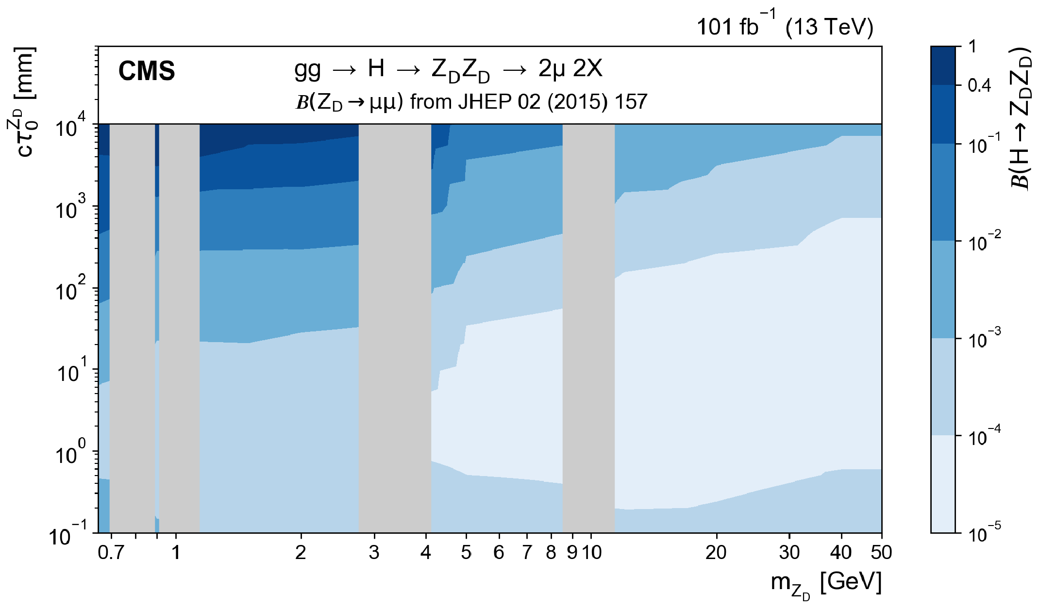
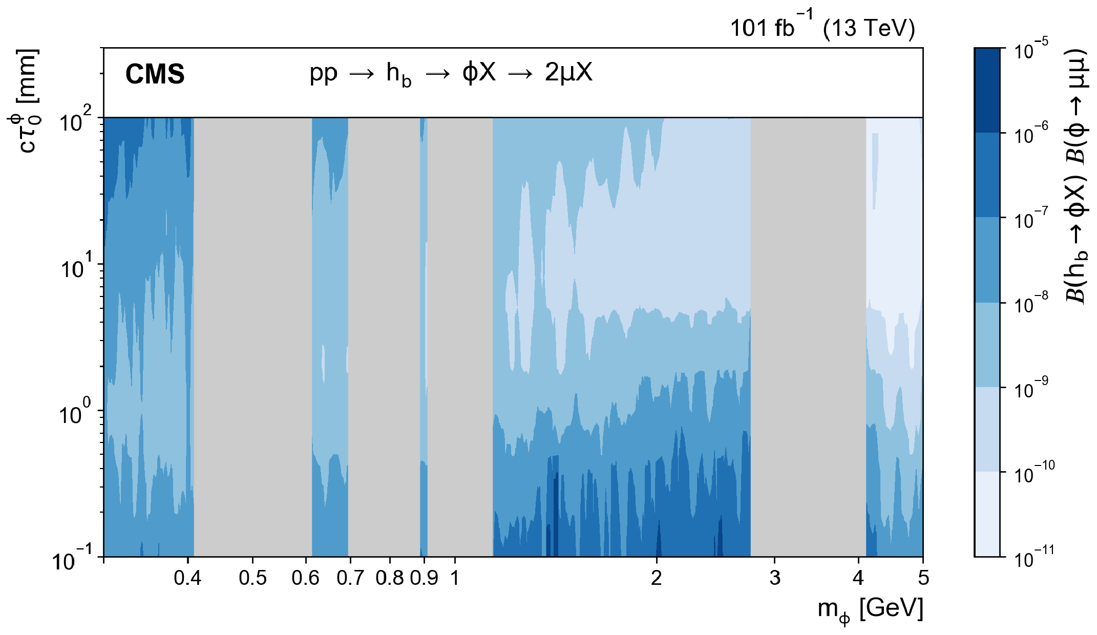
Figure 22:
Observed limits at 95% CL on (upper) the branching fraction $ \mathcal{B}(\mathrm{H} \to \mathrm{Z_D}\mathrm{Z_D}) $ and (lower) the branching fraction product $ {\mathcal{B}(\mathrm{h}_{\mathrm{b}}\to\phi \mathrm{X})\cdot\mathcal{B}(\phi\to\mu\mu)} $ as contours in the parameter space containing the signal mass ($ m_{\mathrm{Z_D}} $ or $ m_{\phi} $, respectively) and the signal lifetime $ c\tau_0 $. The vertical gray bands indicate mass ranges containing known SM resonances, which are masked for this search. The limits are obtained using the combination of all dimuon and four-muon event categories. Figures taken from Ref. [69]. |
png pdf |
Figure 22-a:
Observed limits at 95% CL on (upper) the branching fraction $ \mathcal{B}(\mathrm{H} \to \mathrm{Z_D}\mathrm{Z_D}) $ and (lower) the branching fraction product $ {\mathcal{B}(\mathrm{h}_{\mathrm{b}}\to\phi \mathrm{X})\cdot\mathcal{B}(\phi\to\mu\mu)} $ as contours in the parameter space containing the signal mass ($ m_{\mathrm{Z_D}} $ or $ m_{\phi} $, respectively) and the signal lifetime $ c\tau_0 $. The vertical gray bands indicate mass ranges containing known SM resonances, which are masked for this search. The limits are obtained using the combination of all dimuon and four-muon event categories. Figures taken from Ref. [69]. |
png pdf |
Figure 22-b:
Observed limits at 95% CL on (upper) the branching fraction $ \mathcal{B}(\mathrm{H} \to \mathrm{Z_D}\mathrm{Z_D}) $ and (lower) the branching fraction product $ {\mathcal{B}(\mathrm{h}_{\mathrm{b}}\to\phi \mathrm{X})\cdot\mathcal{B}(\phi\to\mu\mu)} $ as contours in the parameter space containing the signal mass ($ m_{\mathrm{Z_D}} $ or $ m_{\phi} $, respectively) and the signal lifetime $ c\tau_0 $. The vertical gray bands indicate mass ranges containing known SM resonances, which are masked for this search. The limits are obtained using the combination of all dimuon and four-muon event categories. Figures taken from Ref. [69]. |
png pdf |
Figure 23:
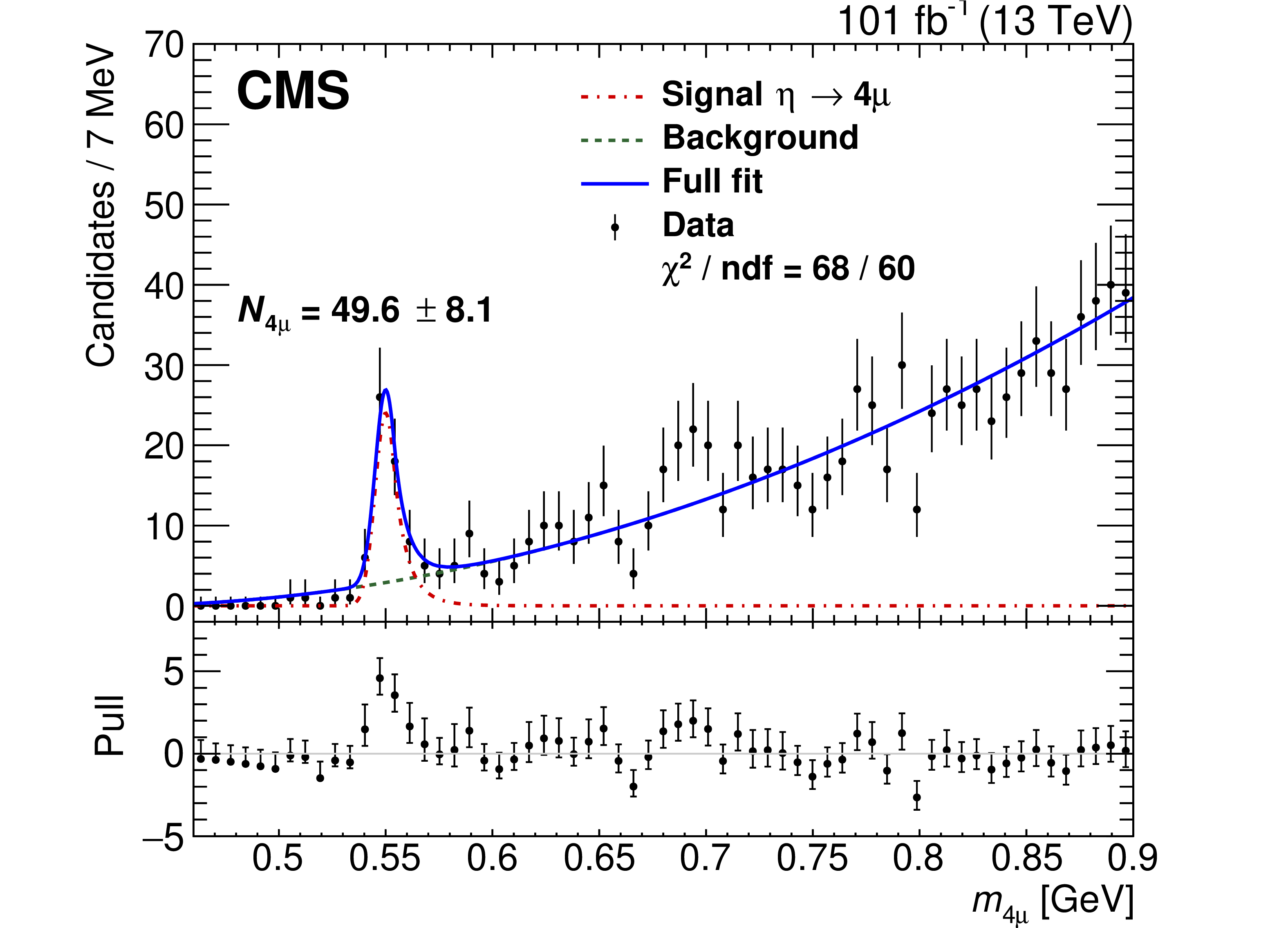
The four-muon invariant mass ($ m_{4\mu} $) distribution in the range 0.46--0.90 GeV, obtained with pp collision data collected during 2017--2018. The observed distribution (points) is compared to the background-only prediction (green dashed) and to the full background fit including simulations of the signal (solid blue). The peak observed in the mass window 0.53--0.57 GeV corresponds to the $ \eta $ meson. The pull distribution in the lower panel is shown relative to the background component of the fit model and defined as $ {(\mathrm{Data} - \mathrm{Fit})/ \mathrm{Uncertainty}} $, where the uncertainty is statistical only. Figure taken from Ref. [95]. |
png pdf |
Figure 24:
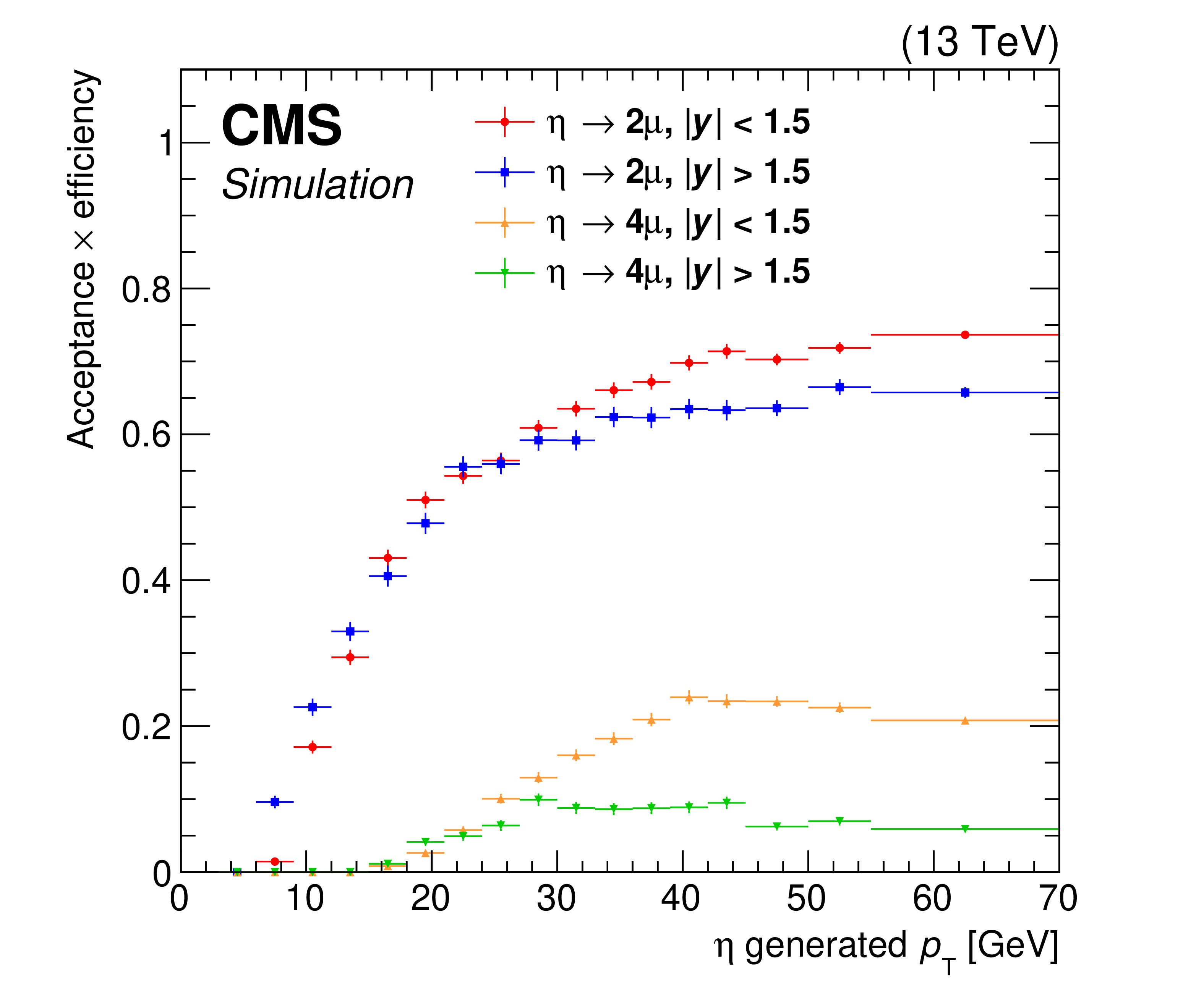
The product of acceptance ($ A $) and efficiency as a function of the generated $ \eta $ meson $ p_{\mathrm{T}} $ for the two-muon (red circles and blue squares) and four-muon (orange up triangles and green down triangles) $ \eta $ meson decays. The product is evaluated using simulated samples. Figure taken from Ref. [95]. |

png pdf |
Figure 25:
Relative rate of each L1 algorithm category, shown as the fraction of the total rate based on the 2022 (orange) and 2023 (blue) configurations. The proportional rate of each category with respect to the total is shown on the right. The values are computed using reference runs with average pileup of 60. |
png pdf |
Figure 26:
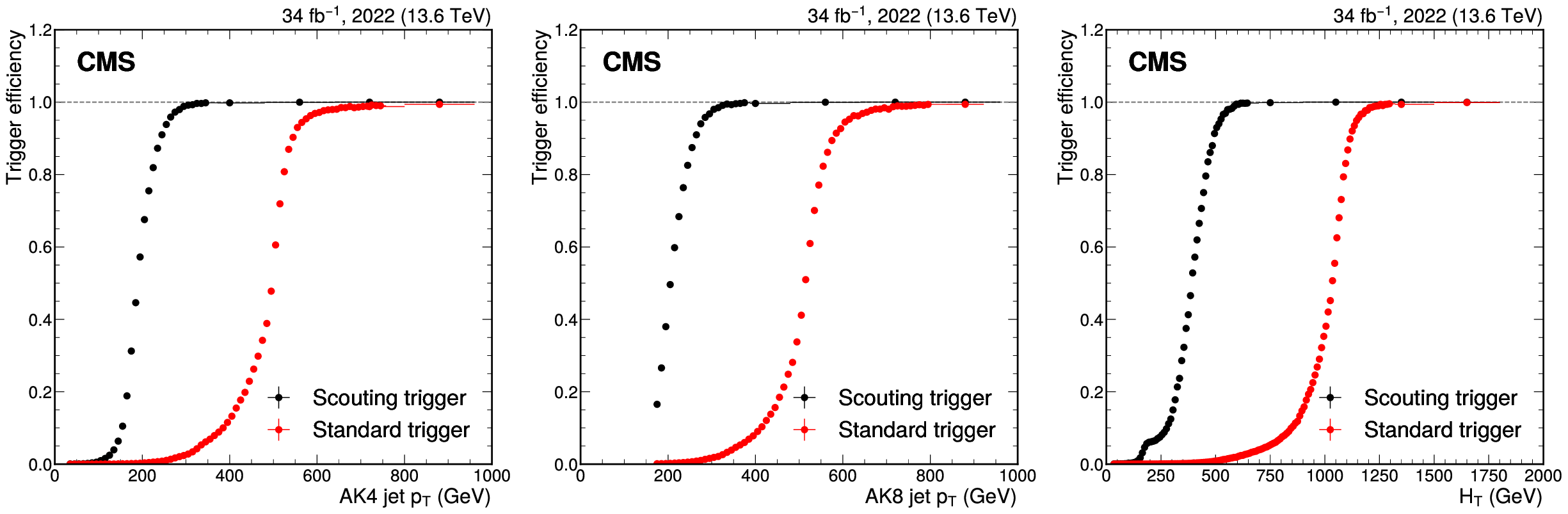
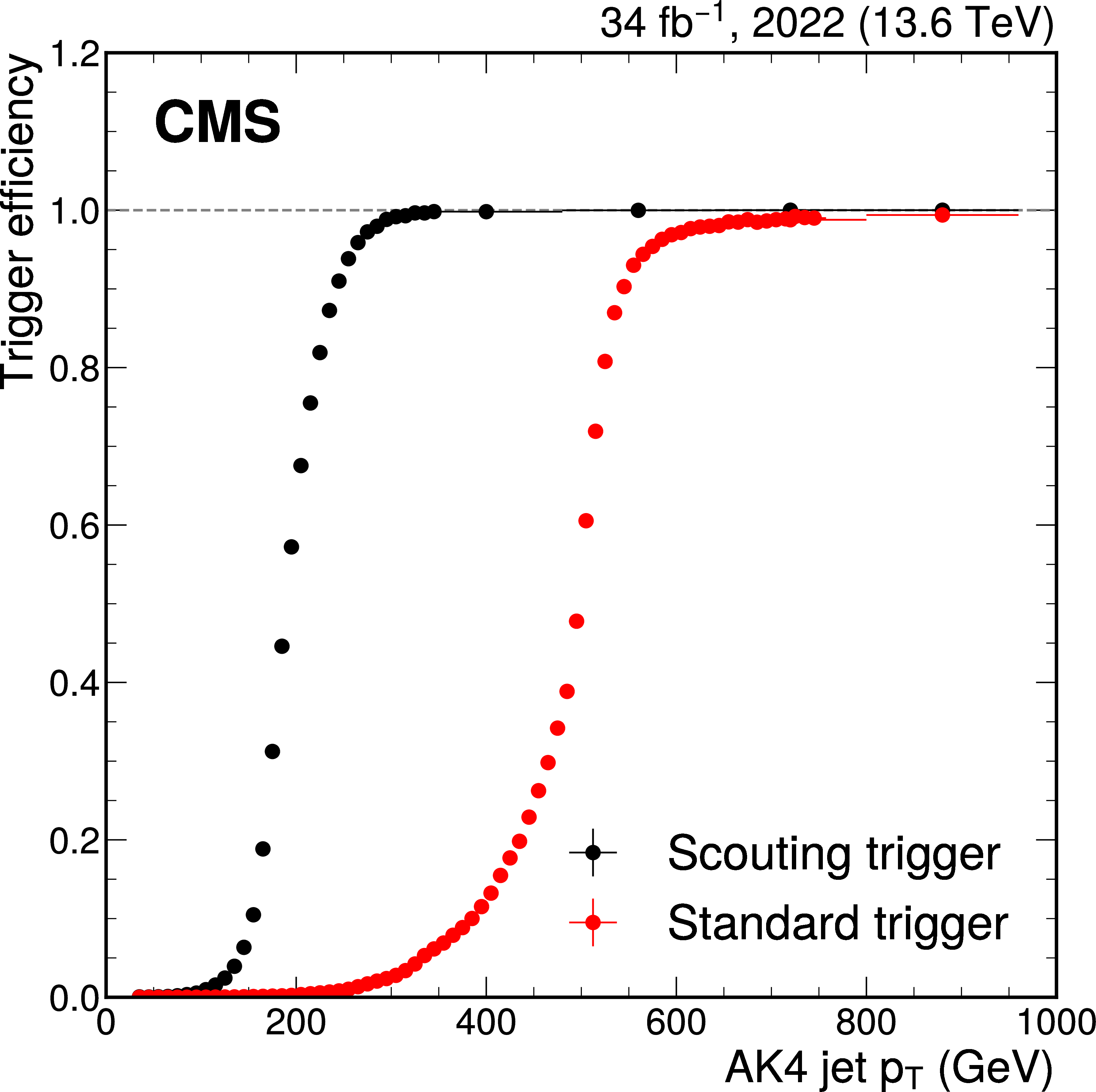
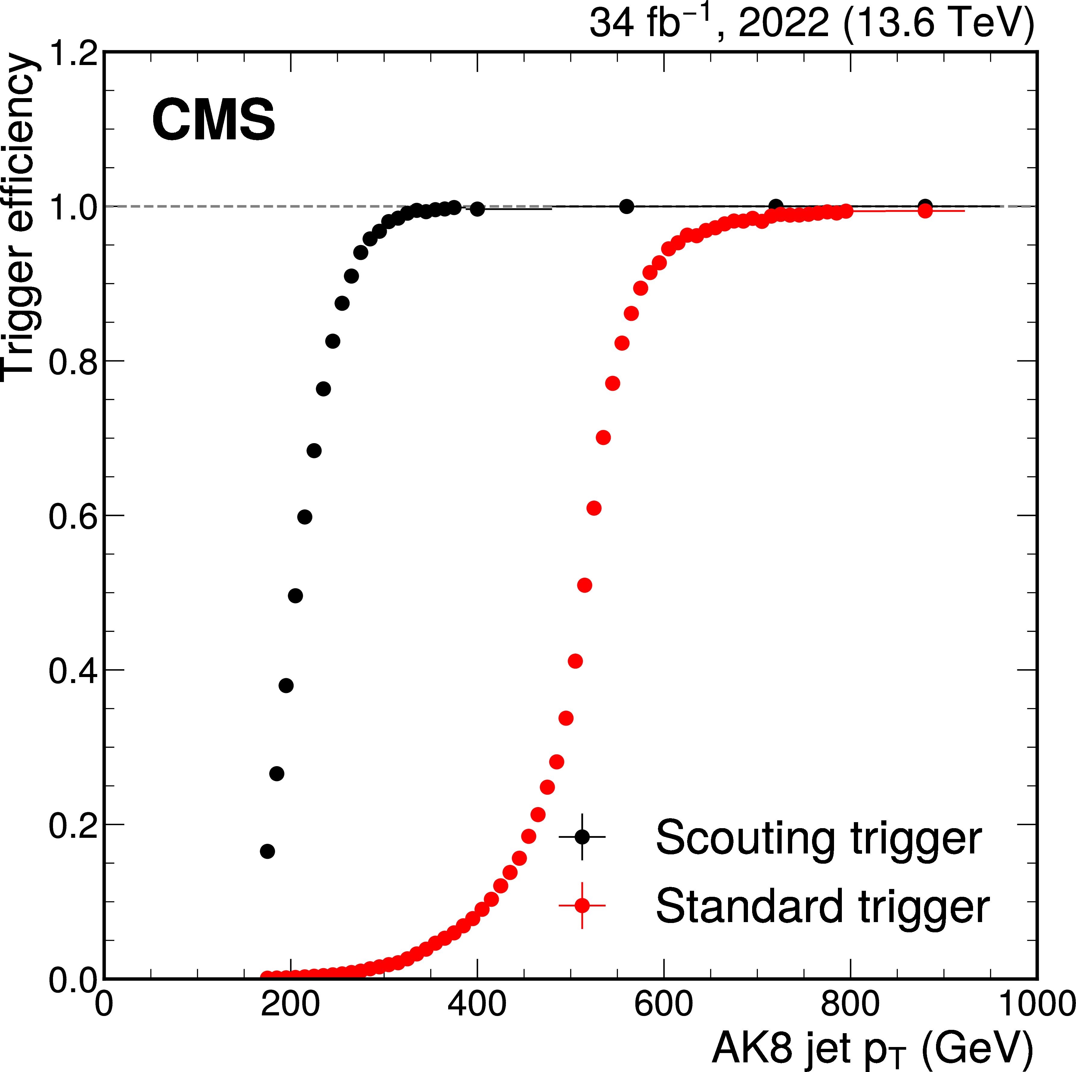
Trigger efficiency as a function of AK4 jet $ p_{\mathrm{T}} $ (left), AK8 jet $ p_{\mathrm{T}} $ (center), and $ H_{\mathrm{T}} $ (right). The efficiency is computed from collision data recorded in 2022 by the scouting (black points) and standard (red points) streams. |
png pdf |
Figure 26-a:
Trigger efficiency as a function of AK4 jet $ p_{\mathrm{T}} $ (left), AK8 jet $ p_{\mathrm{T}} $ (center), and $ H_{\mathrm{T}} $ (right). The efficiency is computed from collision data recorded in 2022 by the scouting (black points) and standard (red points) streams. |
png pdf |
Figure 26-b:
Trigger efficiency as a function of AK4 jet $ p_{\mathrm{T}} $ (left), AK8 jet $ p_{\mathrm{T}} $ (center), and $ H_{\mathrm{T}} $ (right). The efficiency is computed from collision data recorded in 2022 by the scouting (black points) and standard (red points) streams. |

png pdf |
Figure 26-c:
Trigger efficiency as a function of AK4 jet $ p_{\mathrm{T}} $ (left), AK8 jet $ p_{\mathrm{T}} $ (center), and $ H_{\mathrm{T}} $ (right). The efficiency is computed from collision data recorded in 2022 by the scouting (black points) and standard (red points) streams. |
png pdf |
Figure 27:
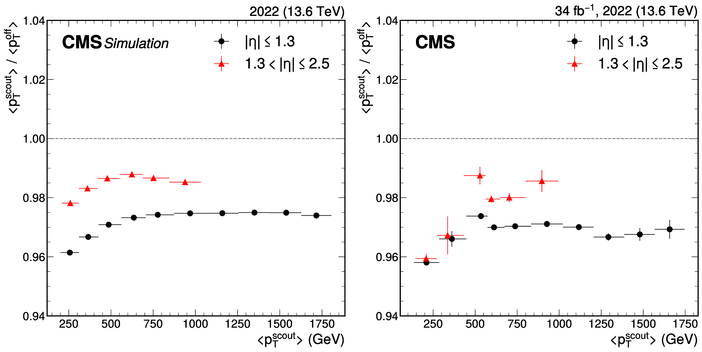
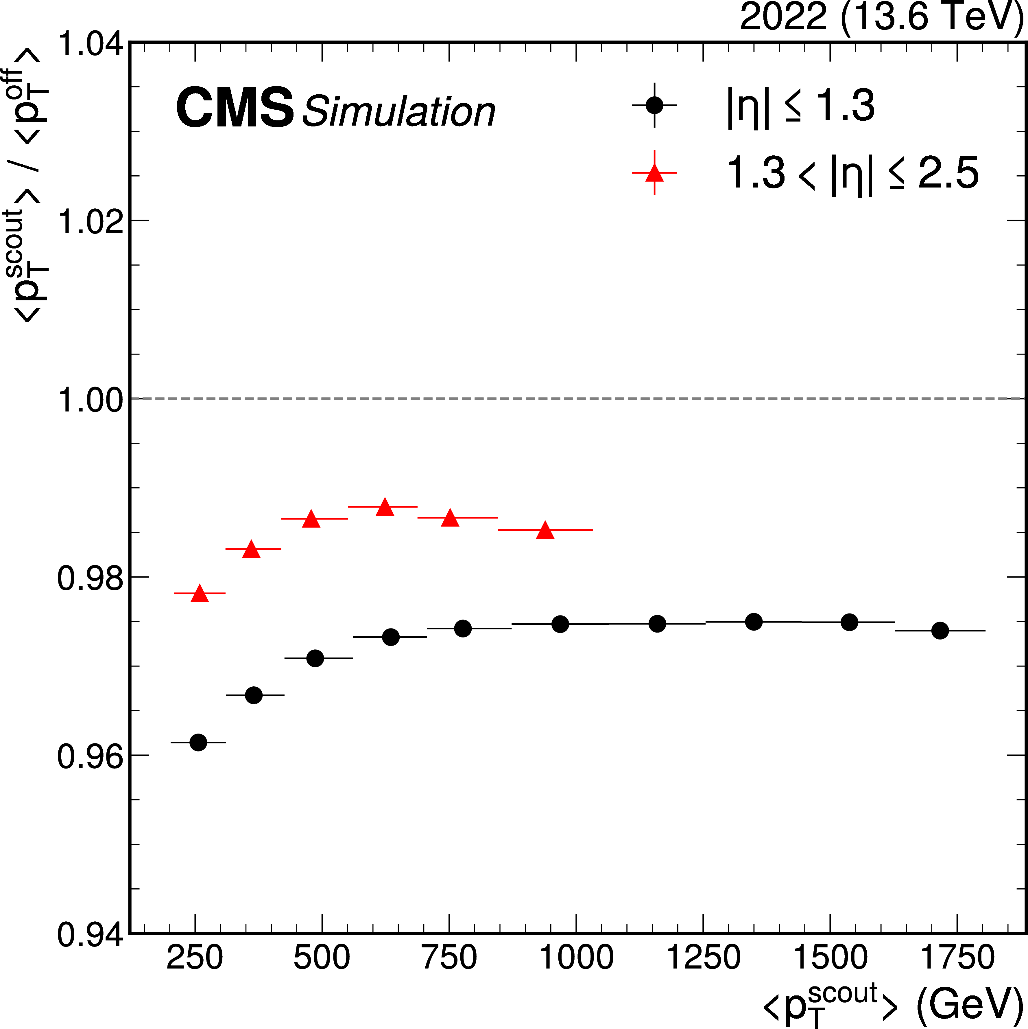
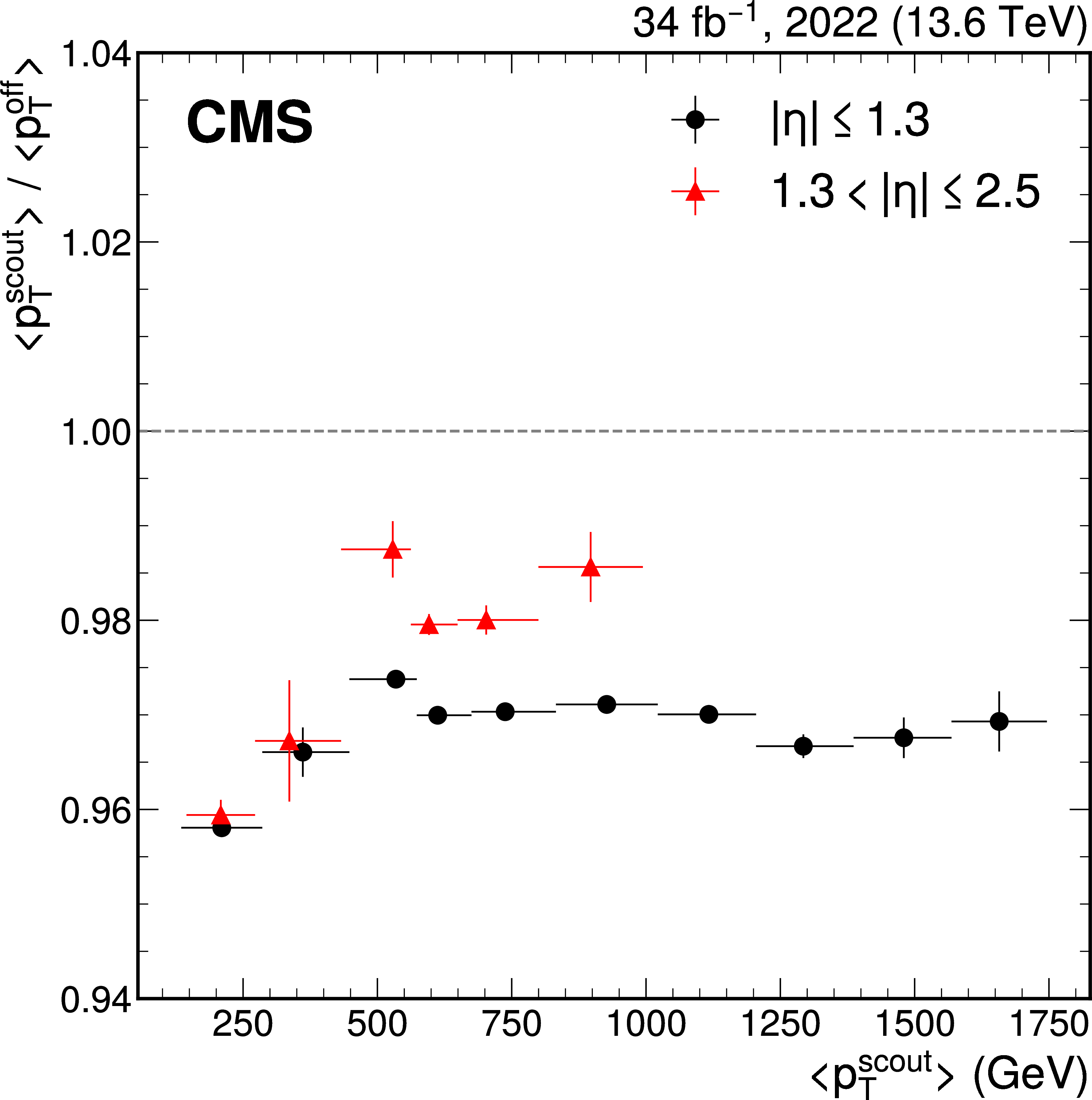
The JES as a function of mean scouting jet $ p_{\mathrm{T}} $ derived from simulated (left) and recorded (right) events. The red and black points correspond to events where the two leading jets have $ {|\eta| } < $ 1.3 and 1.3 $ < |\eta| < $ 2.5, respectively. |
png pdf |
Figure 27-a:
The JES as a function of mean scouting jet $ p_{\mathrm{T}} $ derived from simulated (left) and recorded (right) events. The red and black points correspond to events where the two leading jets have $ {|\eta| } < $ 1.3 and 1.3 $ < |\eta| < $ 2.5, respectively. |
png pdf |
Figure 27-b:
The JES as a function of mean scouting jet $ p_{\mathrm{T}} $ derived from simulated (left) and recorded (right) events. The red and black points correspond to events where the two leading jets have $ {|\eta| } < $ 1.3 and 1.3 $ < |\eta| < $ 2.5, respectively. |
png pdf |
Figure 28:
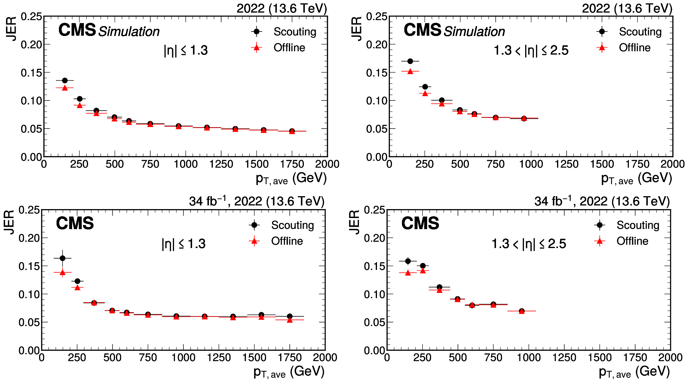
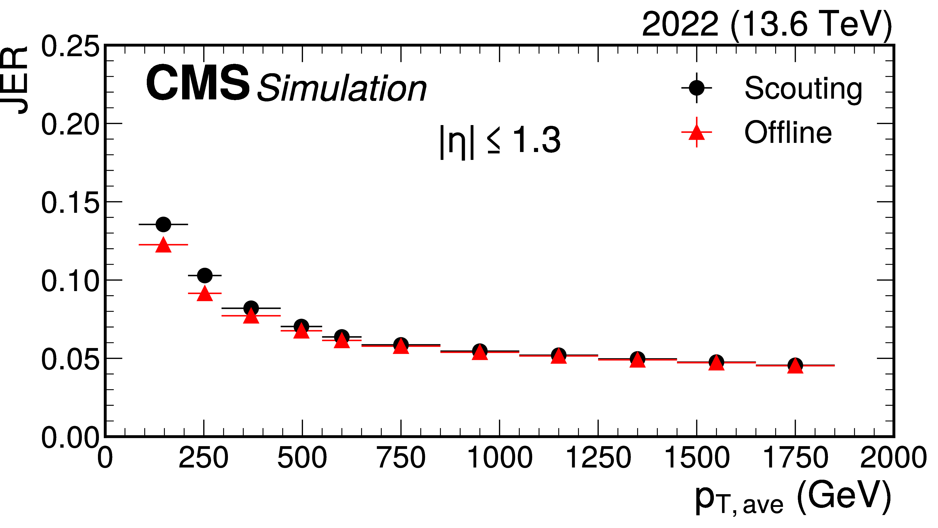
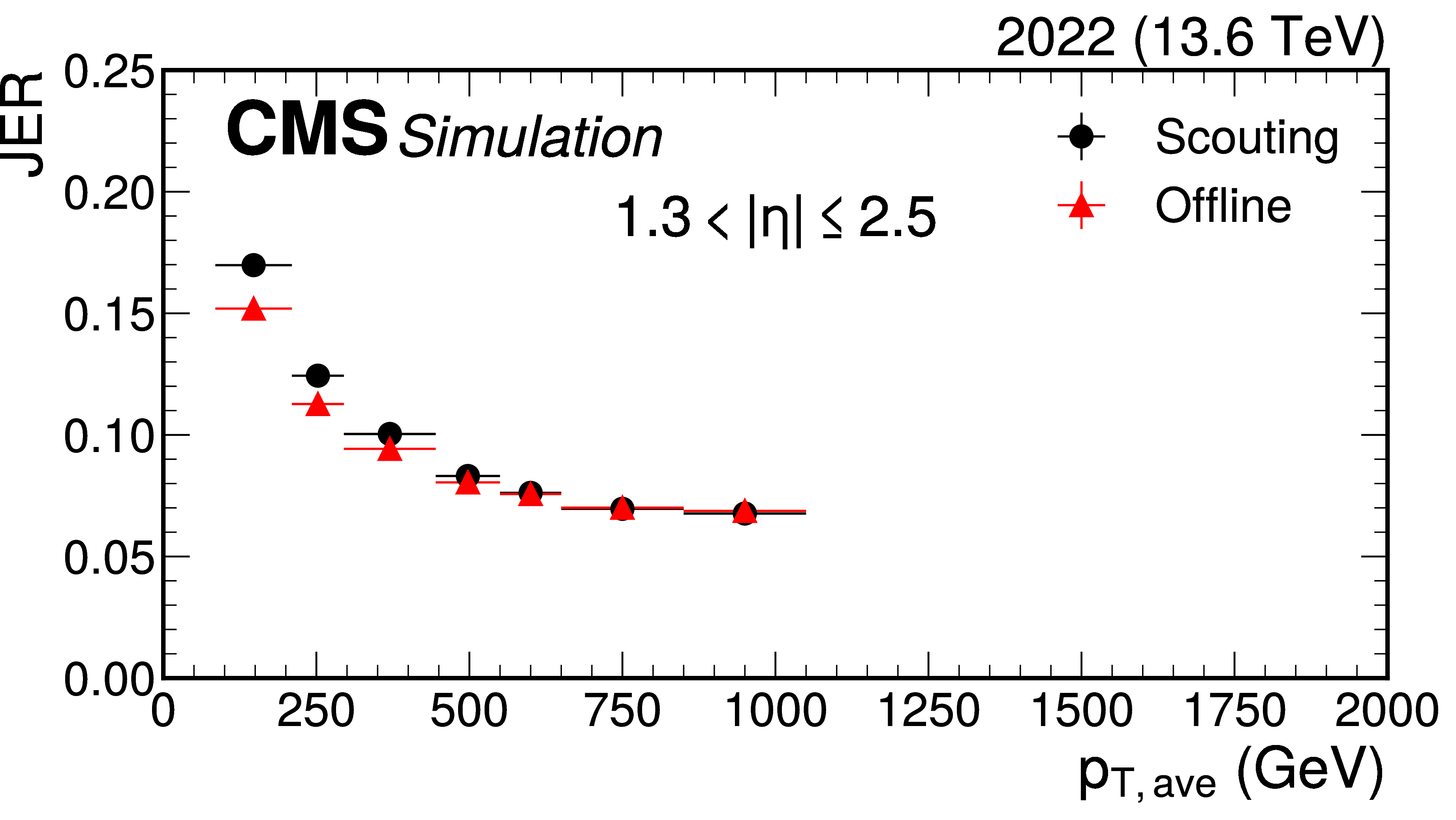
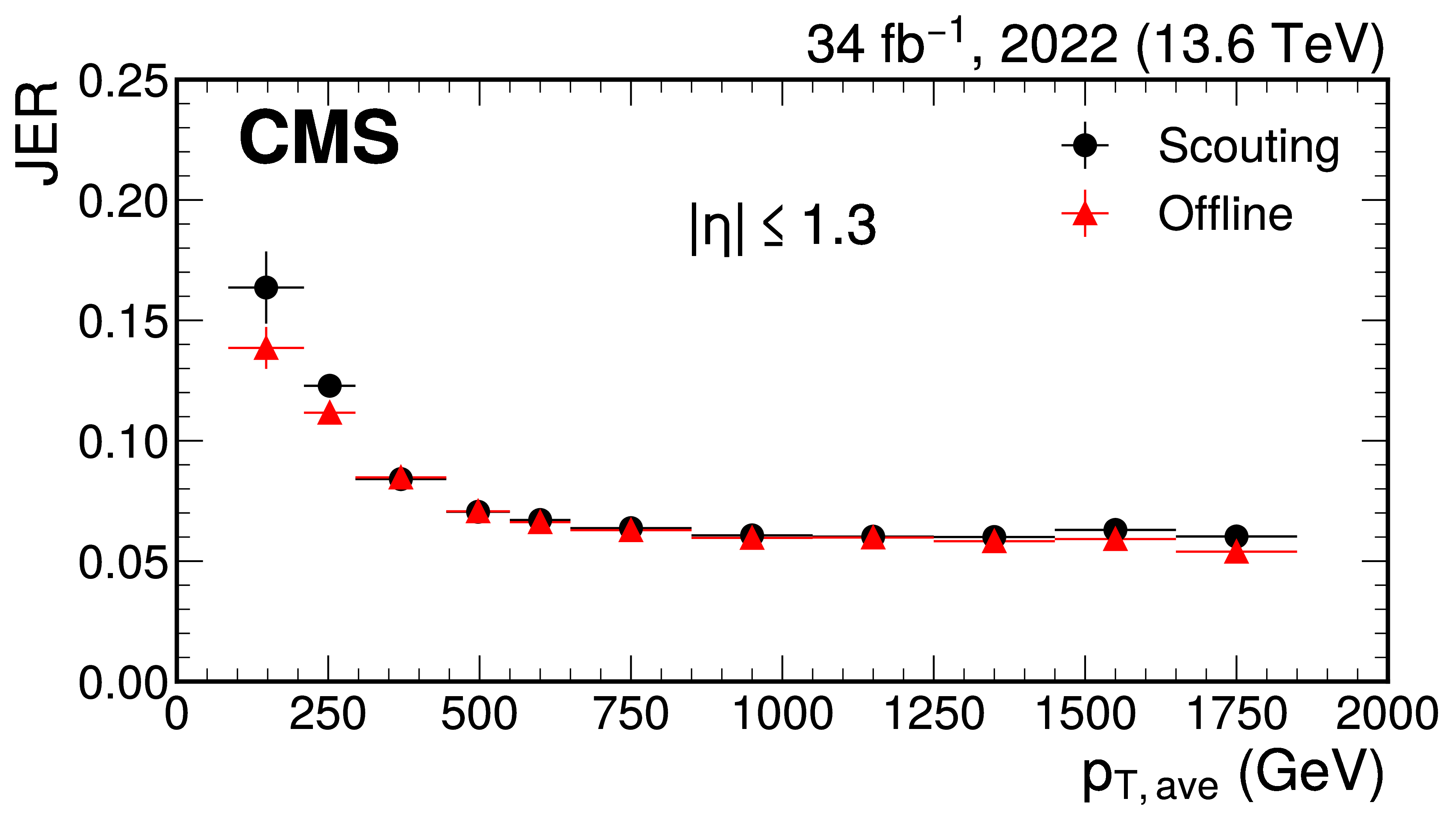
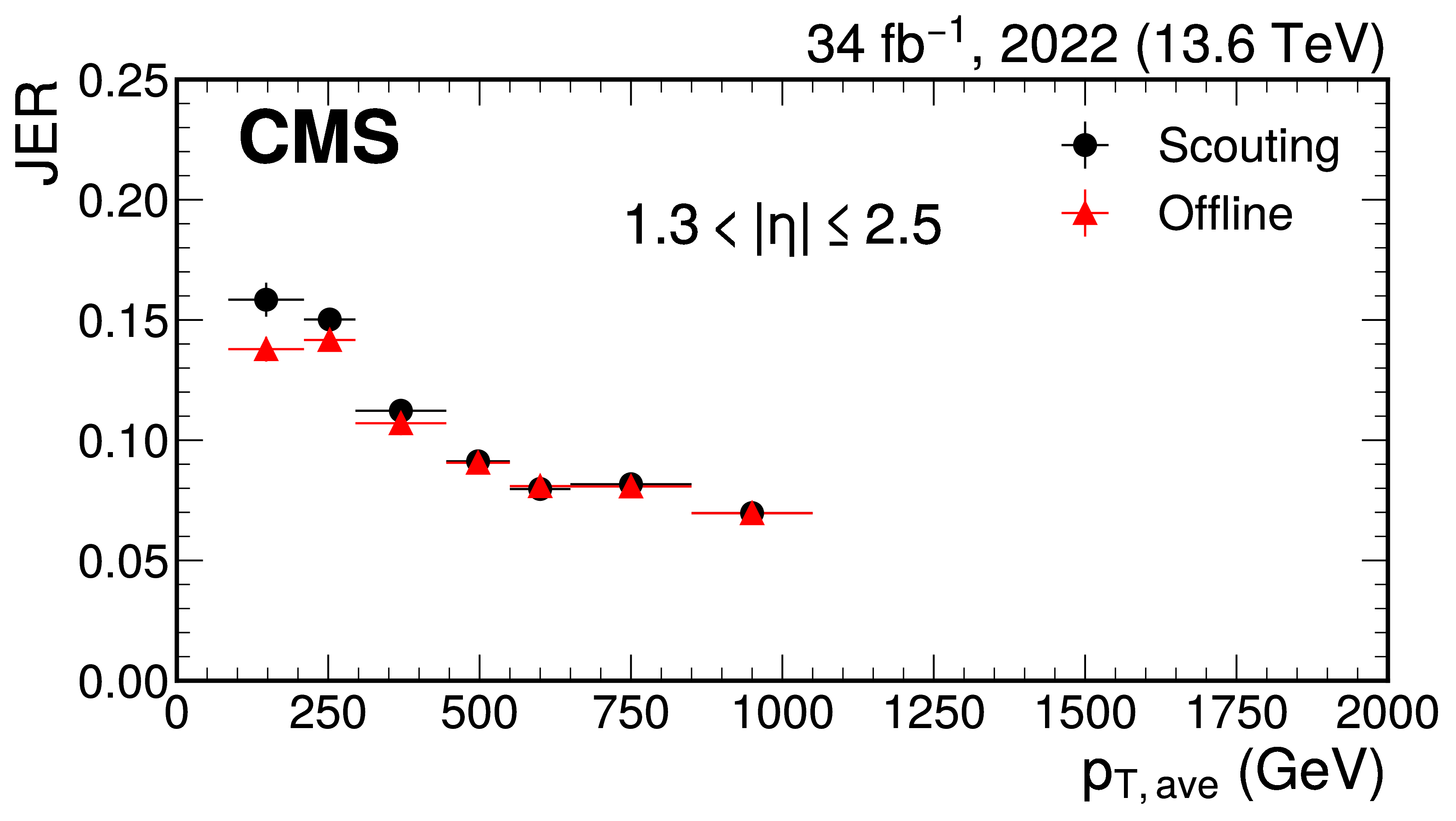
The JER as a function of average $ p_{\mathrm{T}} $. The JER is computed from simulated (upper) and recorded (lower) events, by requiring the two leading jets to have $ |\eta| < $ 1.3 (left) and 1.3 $ < |\eta| < $ 2.5 (right). The red and black data points denote 2022 collision data of the scouting and offline reconstructions, respectively. |
png pdf |
Figure 28-a:
The JER as a function of average $ p_{\mathrm{T}} $. The JER is computed from simulated (upper) and recorded (lower) events, by requiring the two leading jets to have $ |\eta| < $ 1.3 (left) and 1.3 $ < |\eta| < $ 2.5 (right). The red and black data points denote 2022 collision data of the scouting and offline reconstructions, respectively. |
png pdf |
Figure 28-b:
The JER as a function of average $ p_{\mathrm{T}} $. The JER is computed from simulated (upper) and recorded (lower) events, by requiring the two leading jets to have $ |\eta| < $ 1.3 (left) and 1.3 $ < |\eta| < $ 2.5 (right). The red and black data points denote 2022 collision data of the scouting and offline reconstructions, respectively. |
png pdf |
Figure 28-c:
The JER as a function of average $ p_{\mathrm{T}} $. The JER is computed from simulated (upper) and recorded (lower) events, by requiring the two leading jets to have $ |\eta| < $ 1.3 (left) and 1.3 $ < |\eta| < $ 2.5 (right). The red and black data points denote 2022 collision data of the scouting and offline reconstructions, respectively. |
png pdf |
Figure 28-d:
The JER as a function of average $ p_{\mathrm{T}} $. The JER is computed from simulated (upper) and recorded (lower) events, by requiring the two leading jets to have $ |\eta| < $ 1.3 (left) and 1.3 $ < |\eta| < $ 2.5 (right). The red and black data points denote 2022 collision data of the scouting and offline reconstructions, respectively. |

png pdf |
Figure 29:
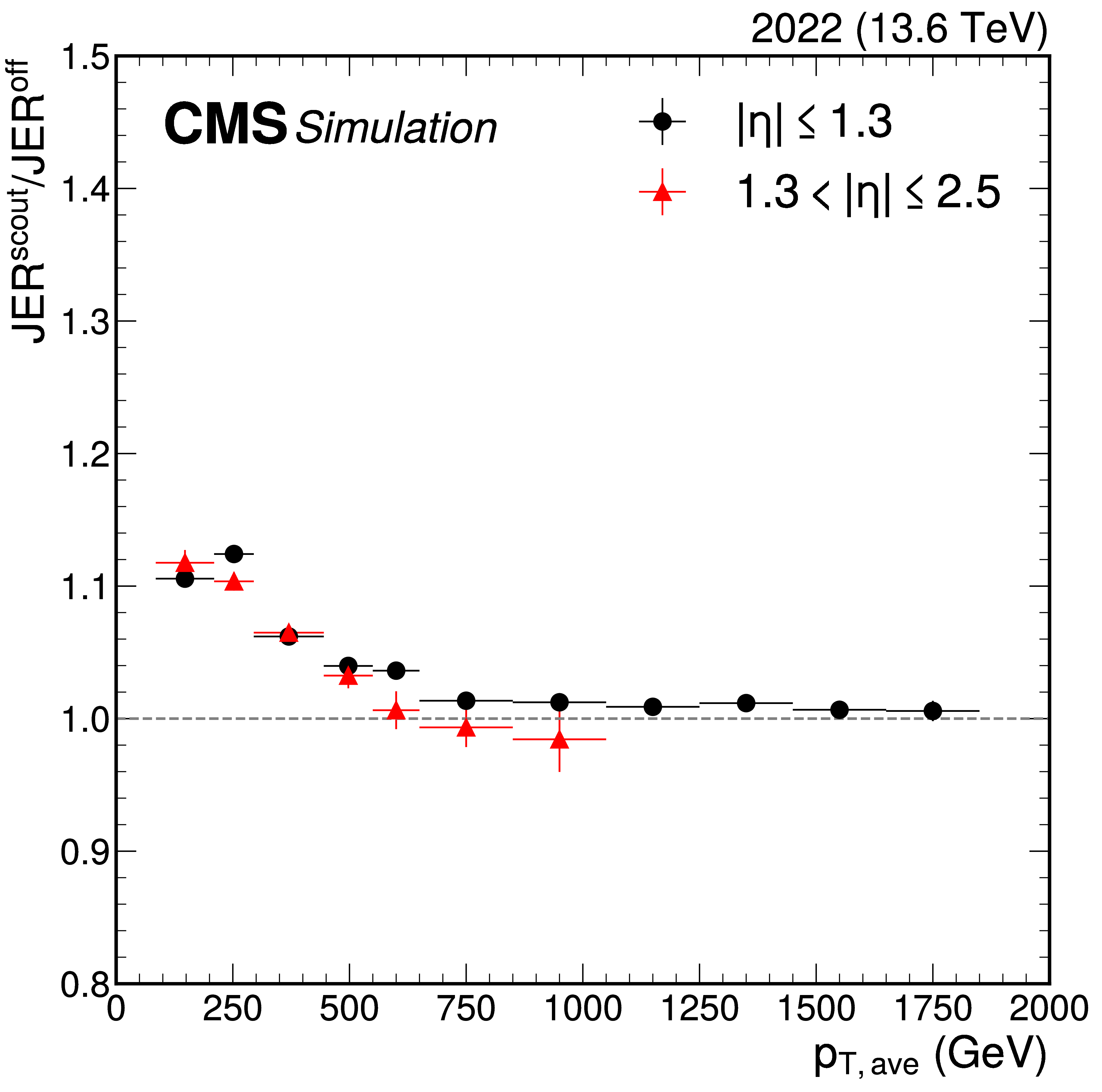
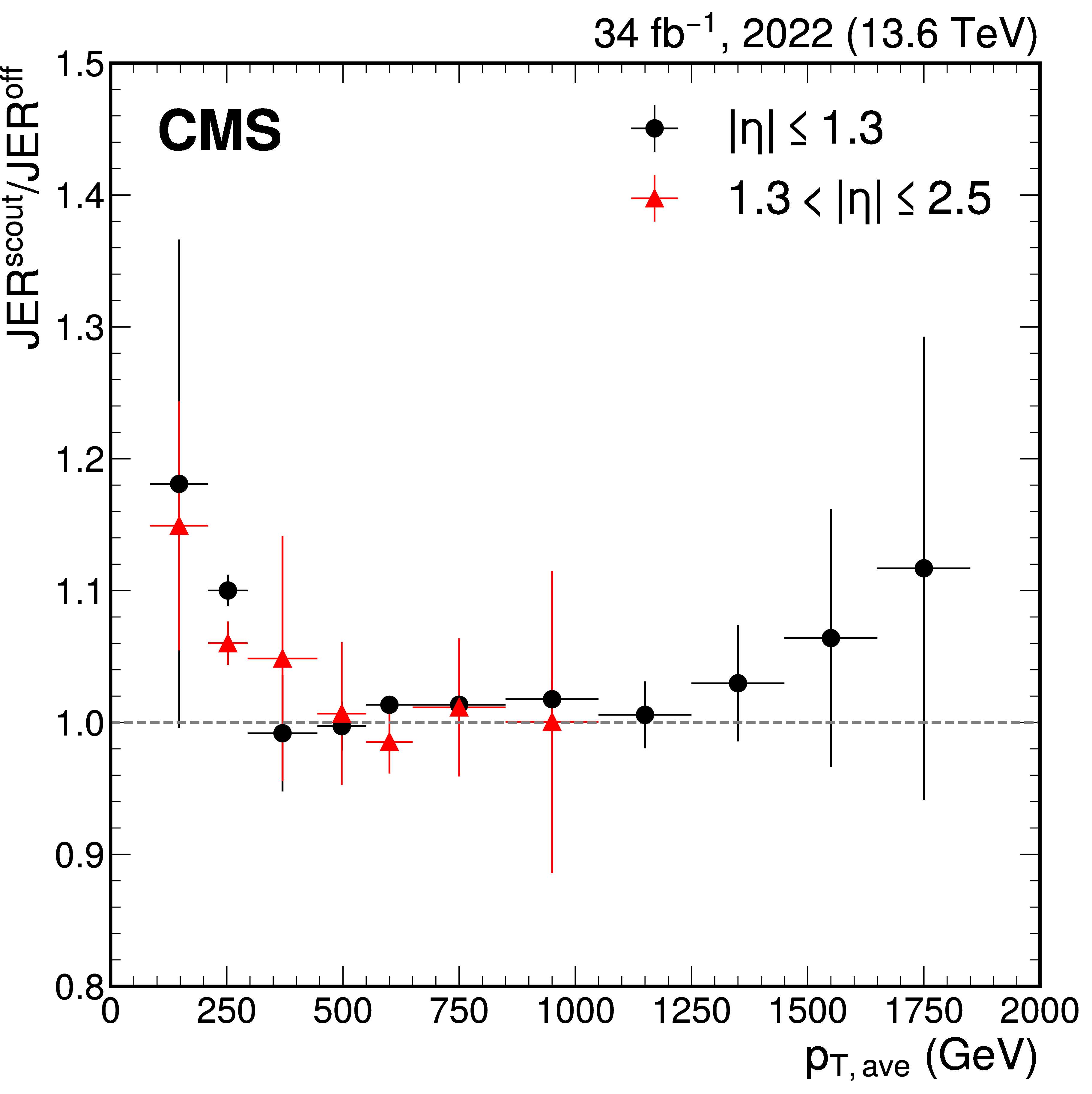
The ratio of the JER derived from scouting events to the JER derived from offline events as a function of average $ p_{\mathrm{T}} $. The ratio is computed from simulated (left) and recorded (right) events, by requiring the two leading jets to have $ |\eta| < $ 1.3 (red points) and 1.3 $ < |\eta| < $ 2.5 (black points). |
png pdf |
Figure 29-a:
The ratio of the JER derived from scouting events to the JER derived from offline events as a function of average $ p_{\mathrm{T}} $. The ratio is computed from simulated (left) and recorded (right) events, by requiring the two leading jets to have $ |\eta| < $ 1.3 (red points) and 1.3 $ < |\eta| < $ 2.5 (black points). |
png pdf |
Figure 29-b:
The ratio of the JER derived from scouting events to the JER derived from offline events as a function of average $ p_{\mathrm{T}} $. The ratio is computed from simulated (left) and recorded (right) events, by requiring the two leading jets to have $ |\eta| < $ 1.3 (red points) and 1.3 $ < |\eta| < $ 2.5 (black points). |

png pdf |
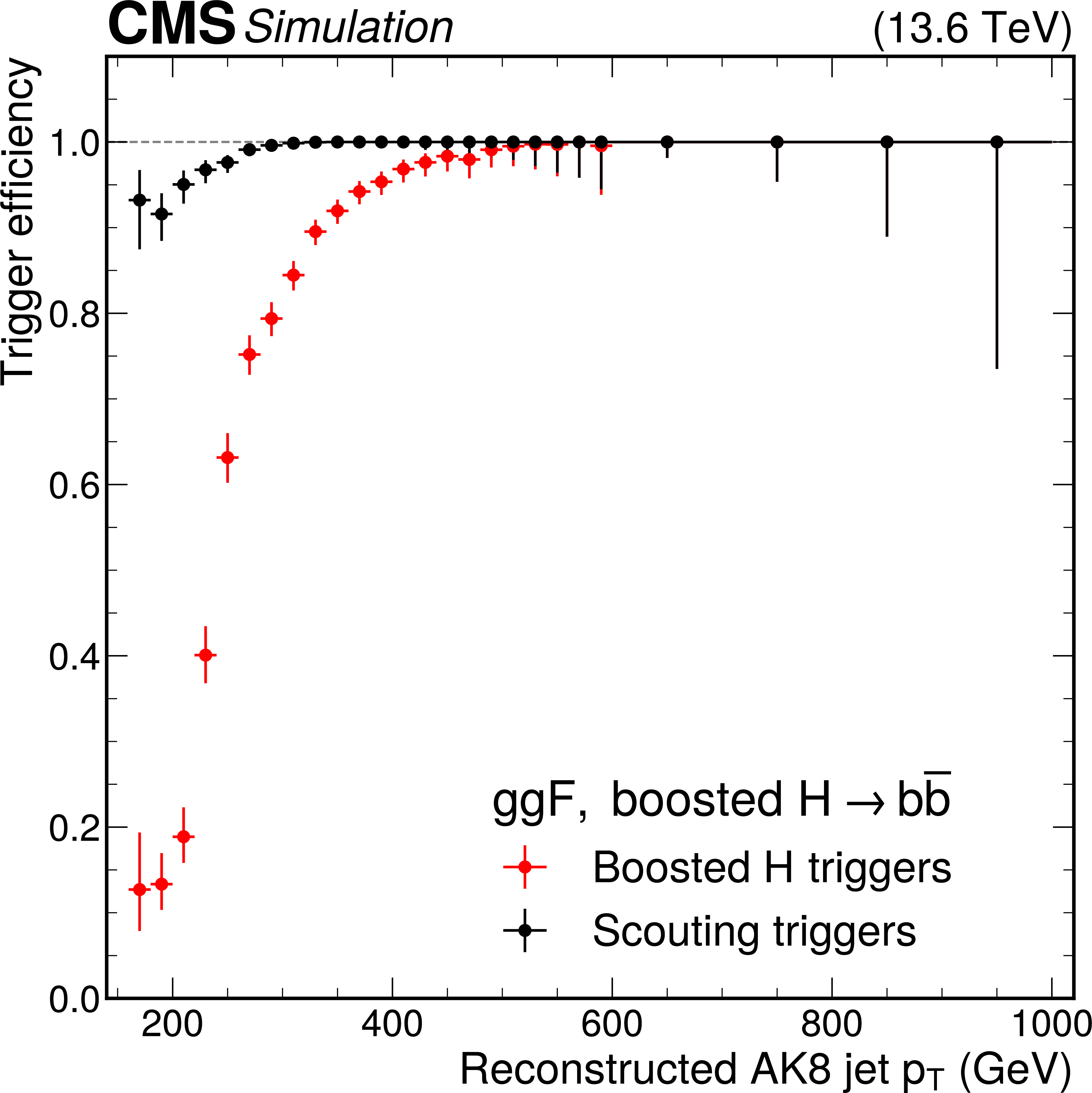
Figure 30:
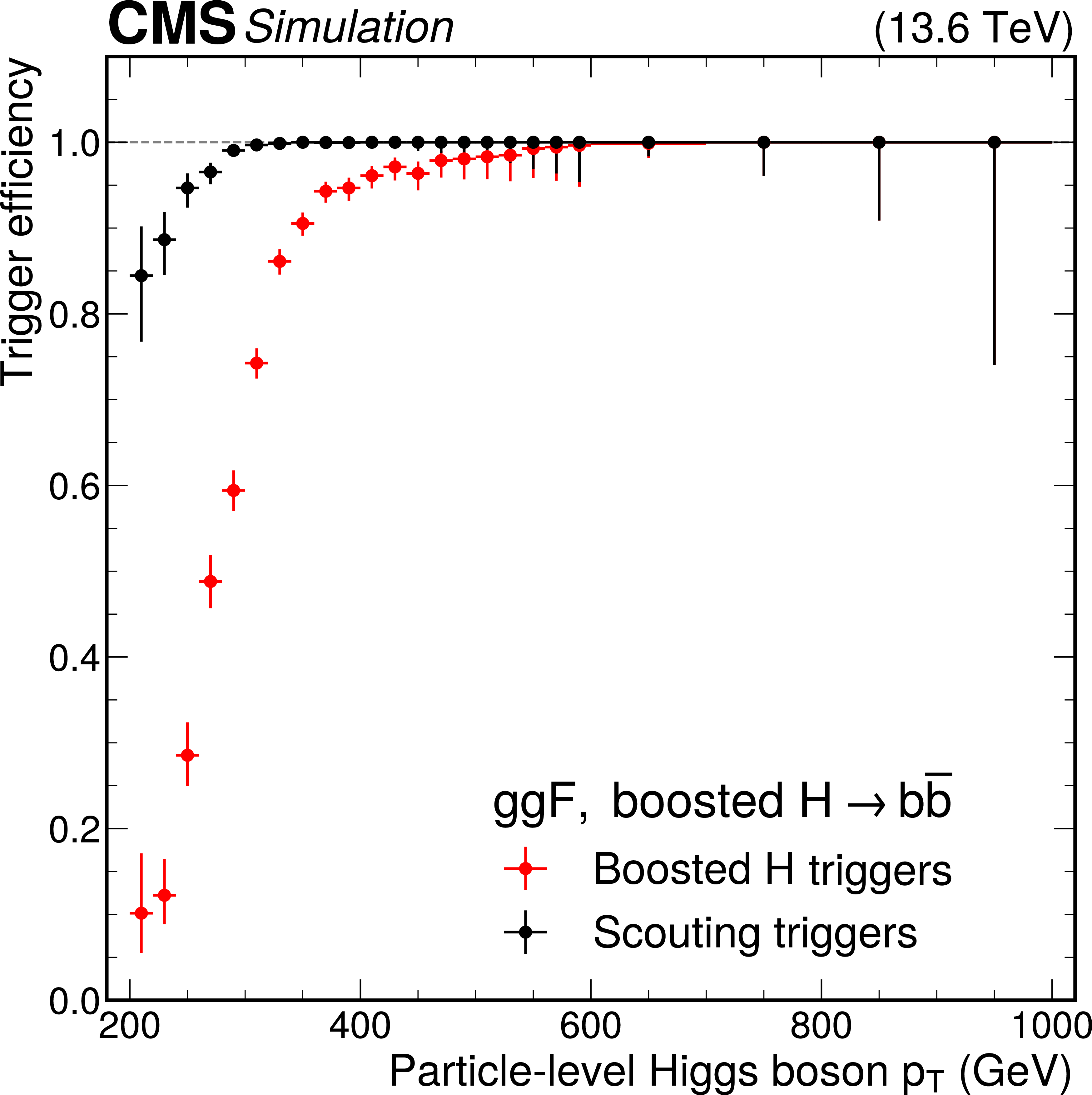
Trigger efficiency for ggF boosted $ \mathrm{H} \to \mathrm{b} \overline{\mathrm{b}} $ events as a function of the highest particle-level Higgs boson $ p_{\mathrm{T}} $ (left) and highest offline-reconstructed AK8 jet $ p_{\mathrm{T}} $ (right), as determined from simulation. The black and red points correspond to the scouting and the standard trigger selection, respectively. |
png pdf |
Figure 30-a:
Trigger efficiency for ggF boosted $ \mathrm{H} \to \mathrm{b} \overline{\mathrm{b}} $ events as a function of the highest particle-level Higgs boson $ p_{\mathrm{T}} $ (left) and highest offline-reconstructed AK8 jet $ p_{\mathrm{T}} $ (right), as determined from simulation. The black and red points correspond to the scouting and the standard trigger selection, respectively. |
png pdf |
Figure 30-b:
Trigger efficiency for ggF boosted $ \mathrm{H} \to \mathrm{b} \overline{\mathrm{b}} $ events as a function of the highest particle-level Higgs boson $ p_{\mathrm{T}} $ (left) and highest offline-reconstructed AK8 jet $ p_{\mathrm{T}} $ (right), as determined from simulation. The black and red points correspond to the scouting and the standard trigger selection, respectively. |
png pdf |
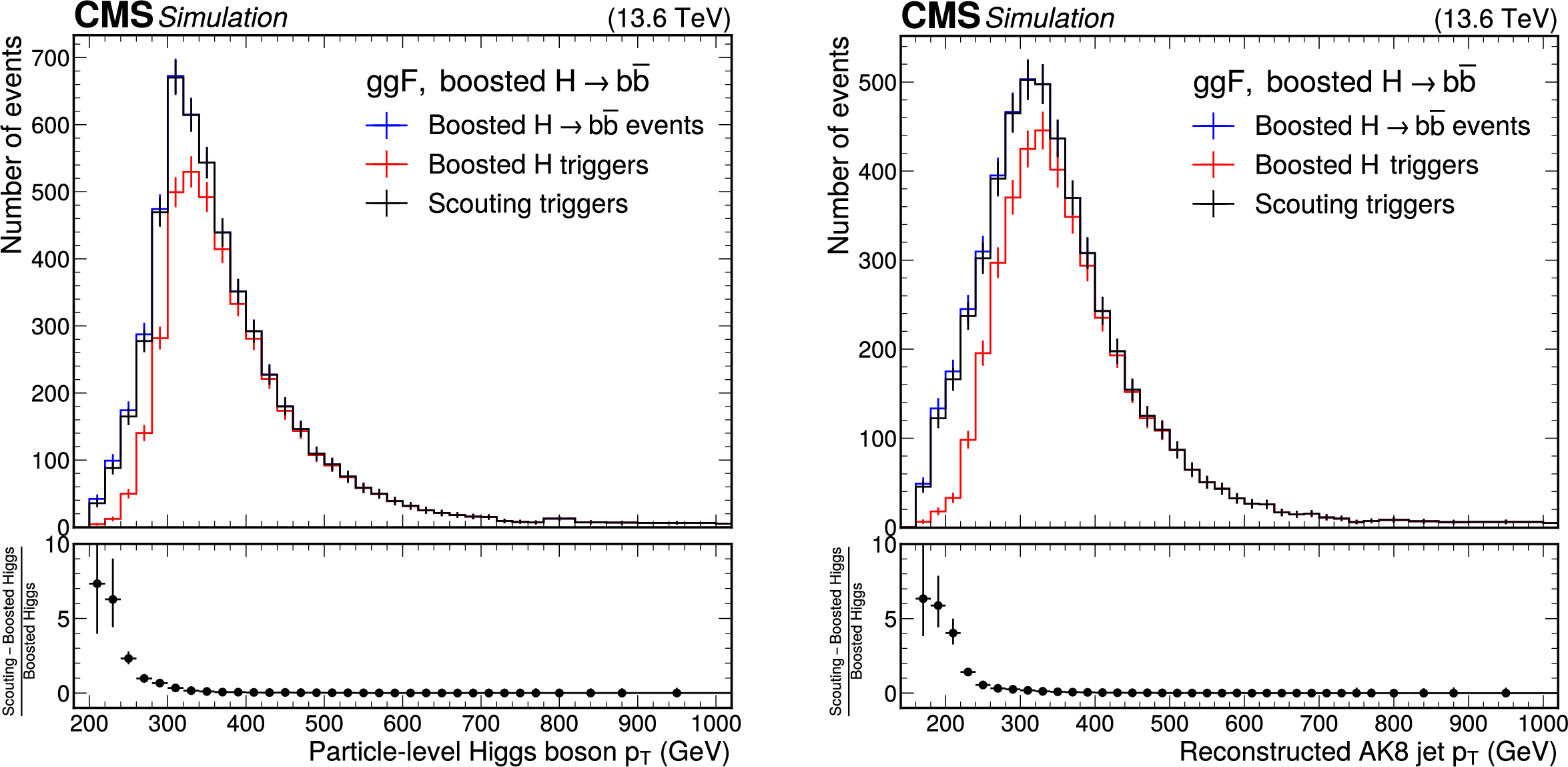
Figure 31:
Number of ggF boosted $ \mathrm{H} \to \mathrm{b} \overline{\mathrm{b}} $ events as a function of the highest particle-level Higgs boson $ p_{\mathrm{T}} $ (left) and highest offline-reconstructed AK8 jet $ p_{\mathrm{T}} $ (right). The large-radius jet with highest $ p_{\mathrm{T}} $ in each event is required to have a maximum angular distance $ {\Delta}R < $ 0.8 from the two final-state b quarks (blue). The events are then required to pass either the standard (red) or scouting (black) trigger selection. The number of events is computed from simulation with projected $ {\mathcal{L}_{\text{int}}} = $ 100 fb$^{-1}$. |

png pdf |
Figure 31-a:
Number of ggF boosted $ \mathrm{H} \to \mathrm{b} \overline{\mathrm{b}} $ events as a function of the highest particle-level Higgs boson $ p_{\mathrm{T}} $ (left) and highest offline-reconstructed AK8 jet $ p_{\mathrm{T}} $ (right). The large-radius jet with highest $ p_{\mathrm{T}} $ in each event is required to have a maximum angular distance $ {\Delta}R < $ 0.8 from the two final-state b quarks (blue). The events are then required to pass either the standard (red) or scouting (black) trigger selection. The number of events is computed from simulation with projected $ {\mathcal{L}_{\text{int}}} = $ 100 fb$^{-1}$. |
png pdf |
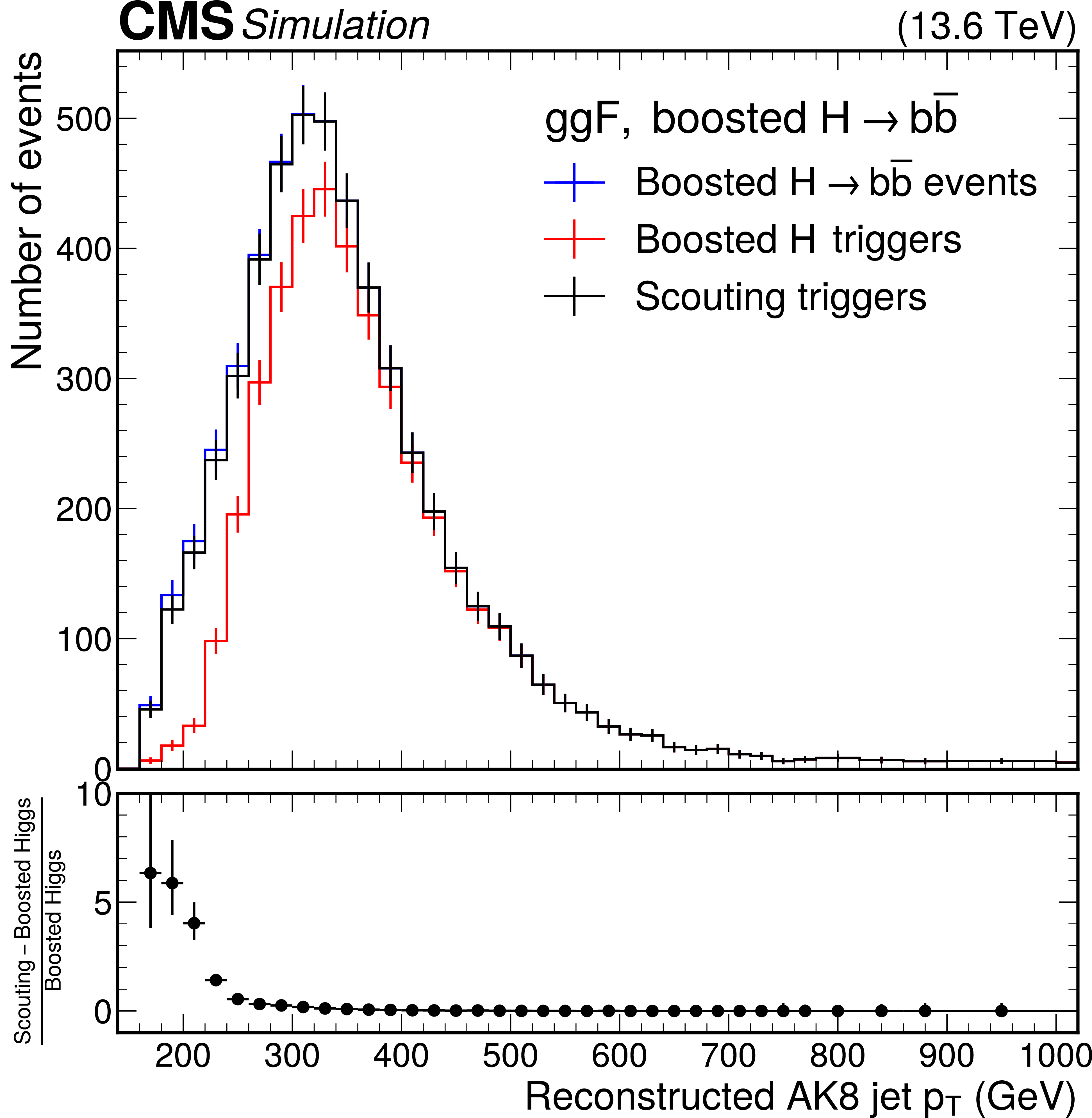
Figure 31-b:
Number of ggF boosted $ \mathrm{H} \to \mathrm{b} \overline{\mathrm{b}} $ events as a function of the highest particle-level Higgs boson $ p_{\mathrm{T}} $ (left) and highest offline-reconstructed AK8 jet $ p_{\mathrm{T}} $ (right). The large-radius jet with highest $ p_{\mathrm{T}} $ in each event is required to have a maximum angular distance $ {\Delta}R < $ 0.8 from the two final-state b quarks (blue). The events are then required to pass either the standard (red) or scouting (black) trigger selection. The number of events is computed from simulation with projected $ {\mathcal{L}_{\text{int}}} = $ 100 fb$^{-1}$. |

png pdf |
Figure 32:
Invariant mass distribution of opposite-sign muon pairs obtained with the scouting triggers, collected during 2022 with all Run 3 dimuon algorithms (blue curve), and with each individual algorithm (remaining colors). |

png pdf |
Figure 33:
Comparison between the $ l_{\text{xy}} $ distribution for Run 2 (orange) and Run 3 (blue) events in data that contain dimuon pairs with a common displaced vertex and a minimal selection on the vertex quality. The dashed vertical lines, placed at radii of 29, 68, 109, and 160$ \,\text{mm} $, correspond to the positions of the pixel layers where photons undergo conversion processes in the material, causing the observed peaks in the $ l_{\text{xy}} $ distribution. |
png pdf |
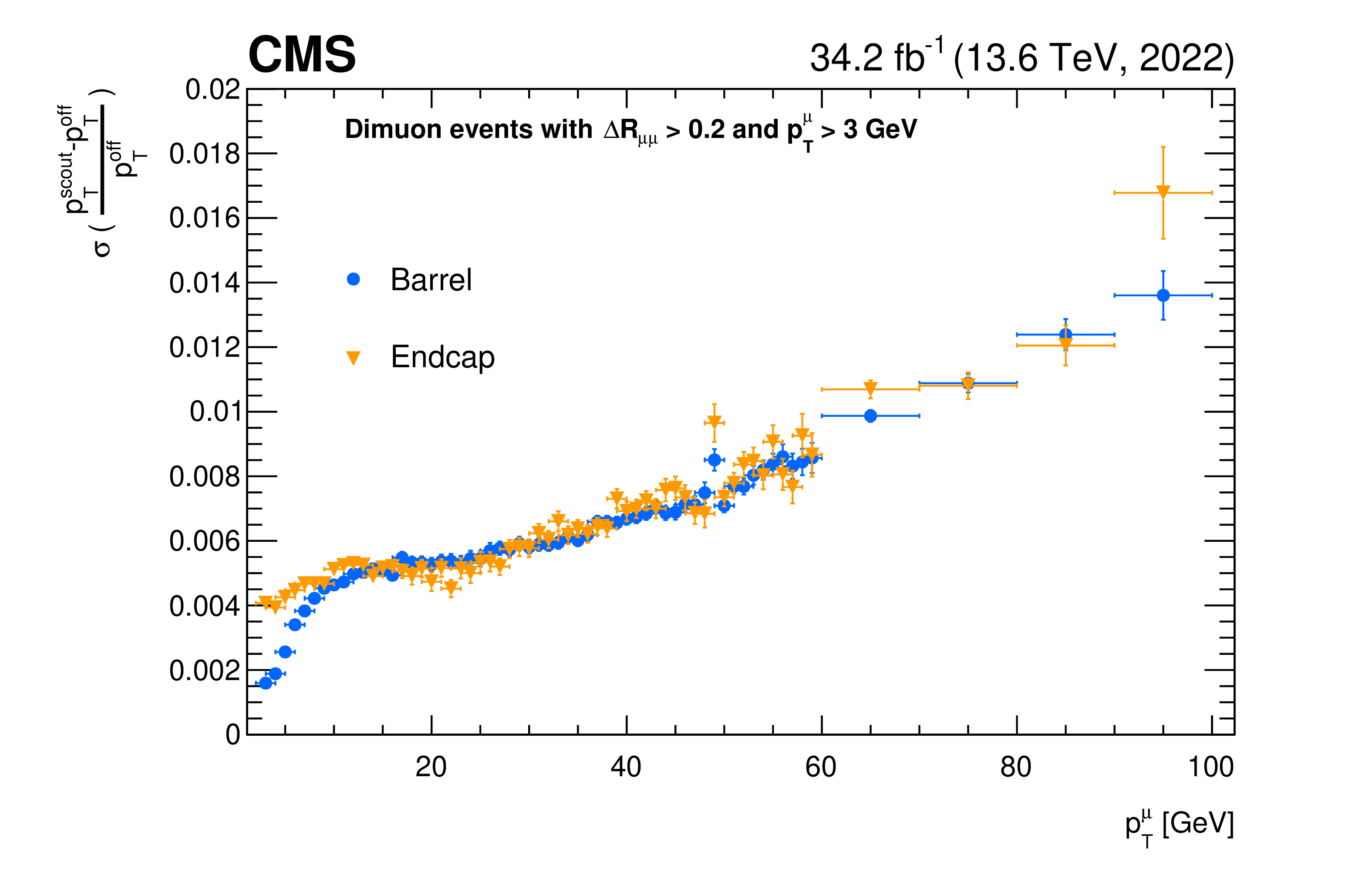
Figure 34:
Resolution on the transverse momentum of scouting muons compared to offline muons using data collected in 2022. Differences in muon momentum scale between the scouting and offline reconstruction algorithms are studied in bins of 1 GeV (10 GeV) for muon $ p_{\mathrm{T}} $ smaller (larger) than 60 GeV. Values for the barrel (blue circles) and endcap (orange triangles) sections are shown separately. |
png pdf |
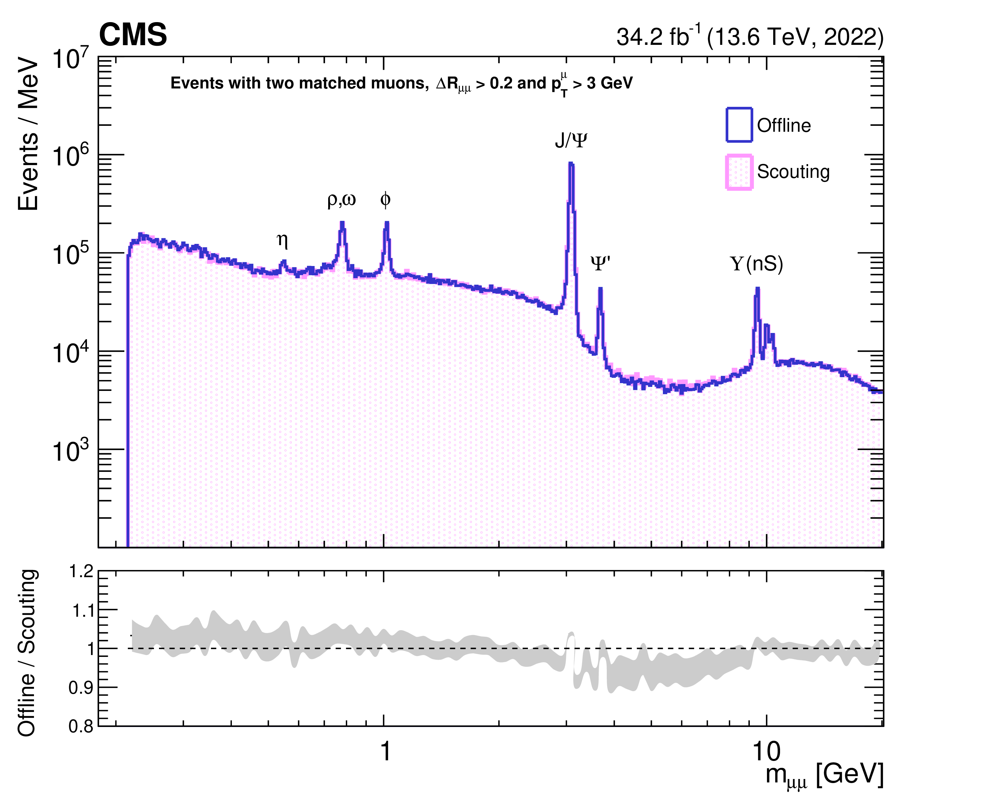
Figure 35:
Comparison of the dimuon spectra obtained with scouting (pink filled histogram) and offline (blue solid line) muons during the 2022 data-taking period. The ratio between the two distributions with a wider binning is also shown in the bottom panel as a gray band. |
png pdf |
Figure 36:
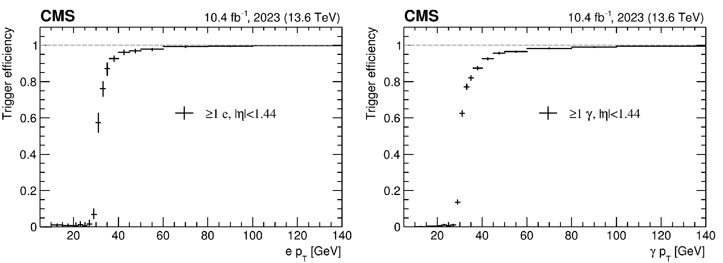
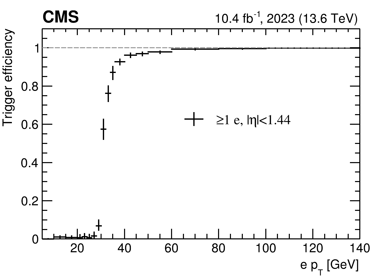
Trigger efficiencies for the scouting trigger paths seeded by L1 algorithms targeting either single-electron events (left) or single-photon events (right), as a function of the respective object $ p_{\mathrm{T}} $ reconstructed offline. To be considered for scouting, the leading electron or photon must have $ {p_{\mathrm{T}}} > $ 30 GeV. Results are only shown for electrons or photons detected in the barrel region. |
png |
Figure 36-a:
Trigger efficiencies for the scouting trigger paths seeded by L1 algorithms targeting either single-electron events (left) or single-photon events (right), as a function of the respective object $ p_{\mathrm{T}} $ reconstructed offline. To be considered for scouting, the leading electron or photon must have $ {p_{\mathrm{T}}} > $ 30 GeV. Results are only shown for electrons or photons detected in the barrel region. |

png |
Figure 36-b:
Trigger efficiencies for the scouting trigger paths seeded by L1 algorithms targeting either single-electron events (left) or single-photon events (right), as a function of the respective object $ p_{\mathrm{T}} $ reconstructed offline. To be considered for scouting, the leading electron or photon must have $ {p_{\mathrm{T}}} > $ 30 GeV. Results are only shown for electrons or photons detected in the barrel region. |
png pdf |
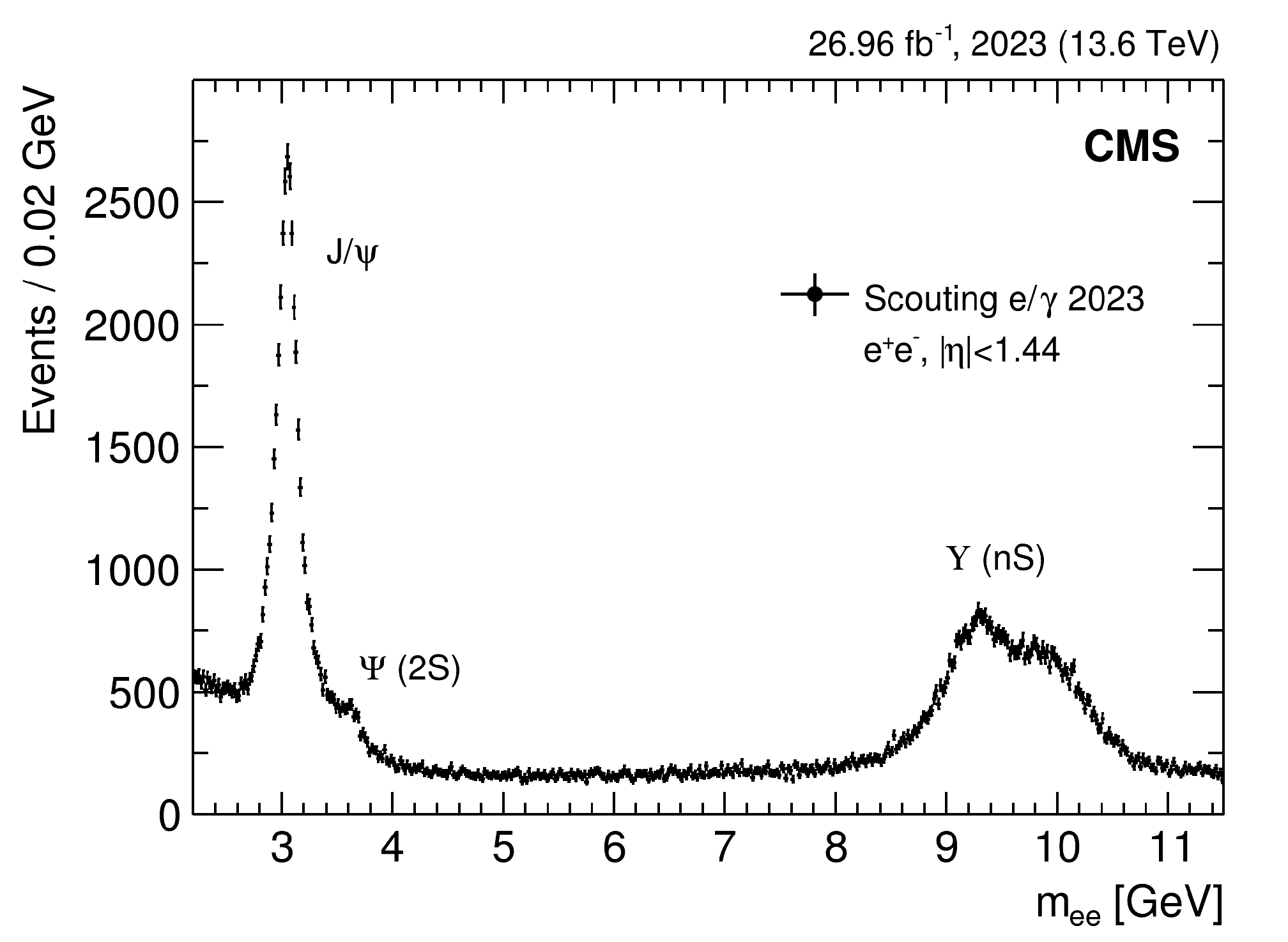
Figure 37:
Dielectron mass distribution observed with Run 3 scouting data collected during the 2023 data-taking period. The $ \mathrm{J}/\psi $ and two of the $ \Upsilon $ meson peaks are visible. |
png pdf |
Figure 38:
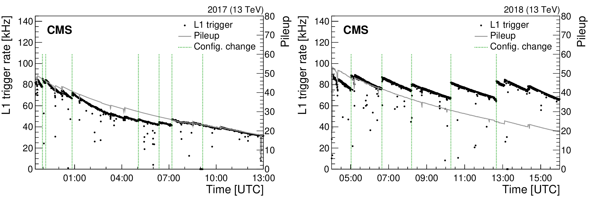
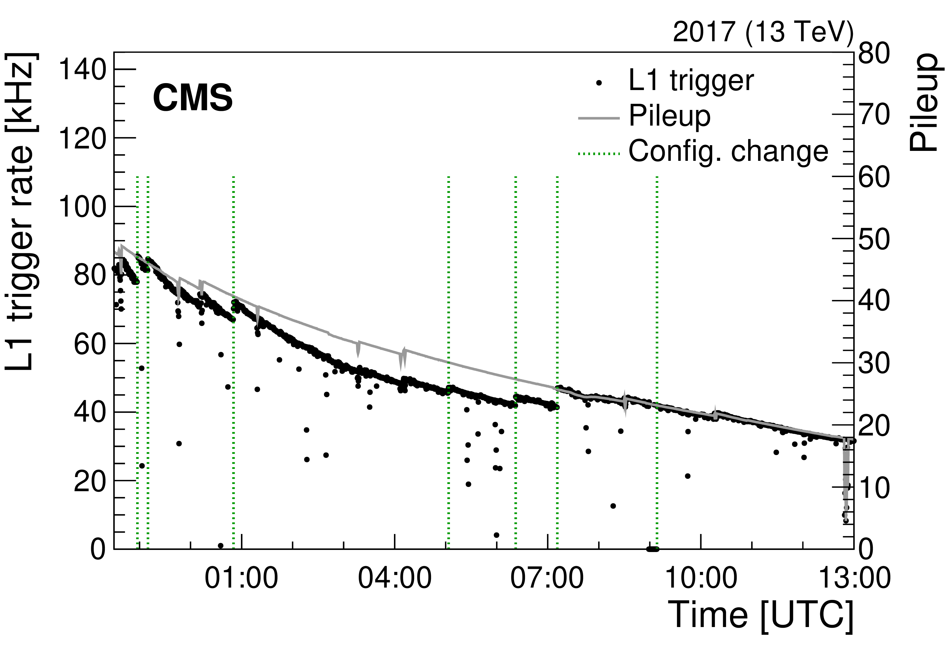
The L1 trigger rate and the amount of pileup as a function of time, shown for representative LHC fills during 2017 (left) and 2018 (right). Occasional lower rates are observed due to transient effects, such as the throttling of the trigger system in response to subdetector dead time [9]. Changes in the trigger configuration are indicated by vertical green dashed lines. |
png pdf |
Figure 38-a:
The L1 trigger rate and the amount of pileup as a function of time, shown for representative LHC fills during 2017 (left) and 2018 (right). Occasional lower rates are observed due to transient effects, such as the throttling of the trigger system in response to subdetector dead time [9]. Changes in the trigger configuration are indicated by vertical green dashed lines. |

png pdf |
Figure 38-b:
The L1 trigger rate and the amount of pileup as a function of time, shown for representative LHC fills during 2017 (left) and 2018 (right). Occasional lower rates are observed due to transient effects, such as the throttling of the trigger system in response to subdetector dead time [9]. Changes in the trigger configuration are indicated by vertical green dashed lines. |

png pdf |
Figure 39:
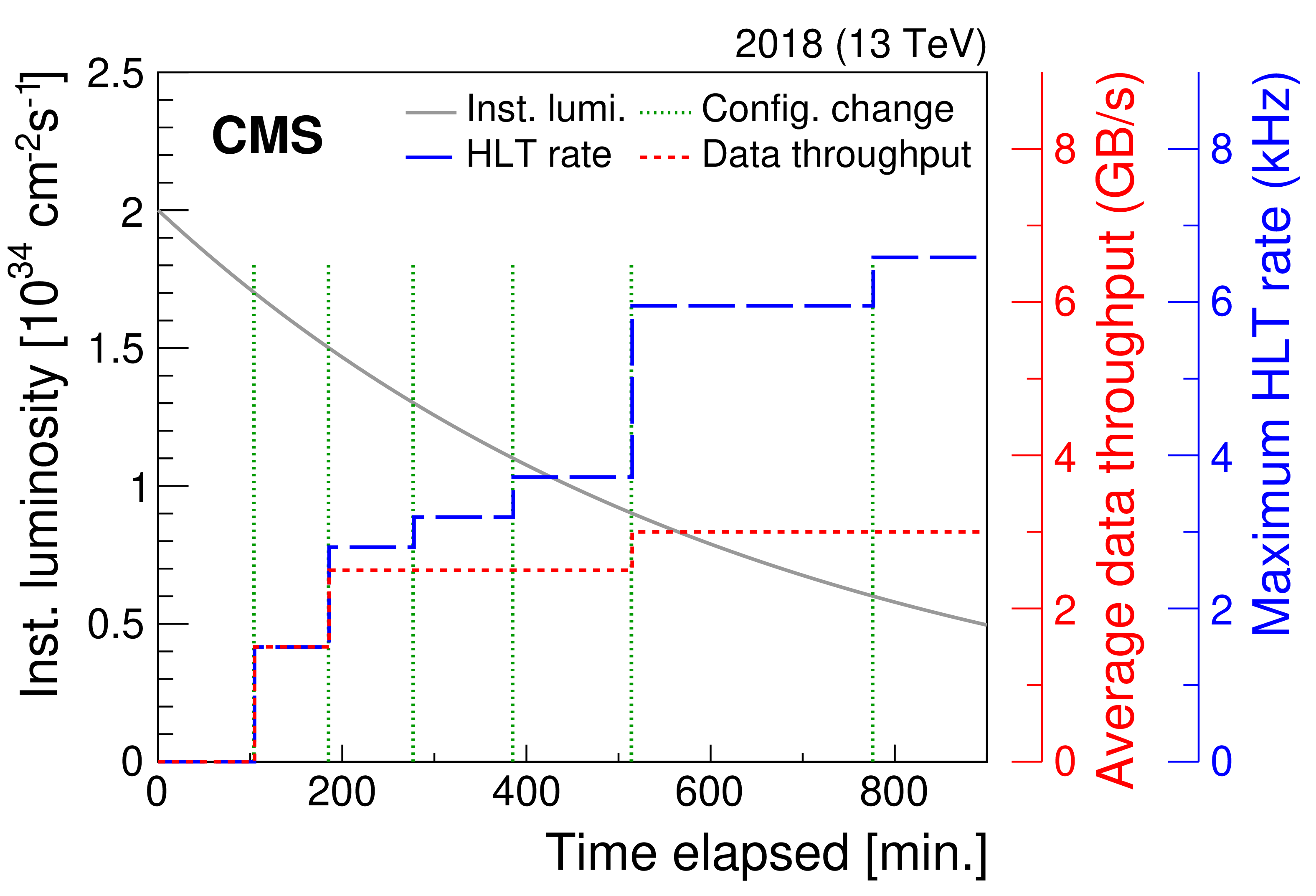
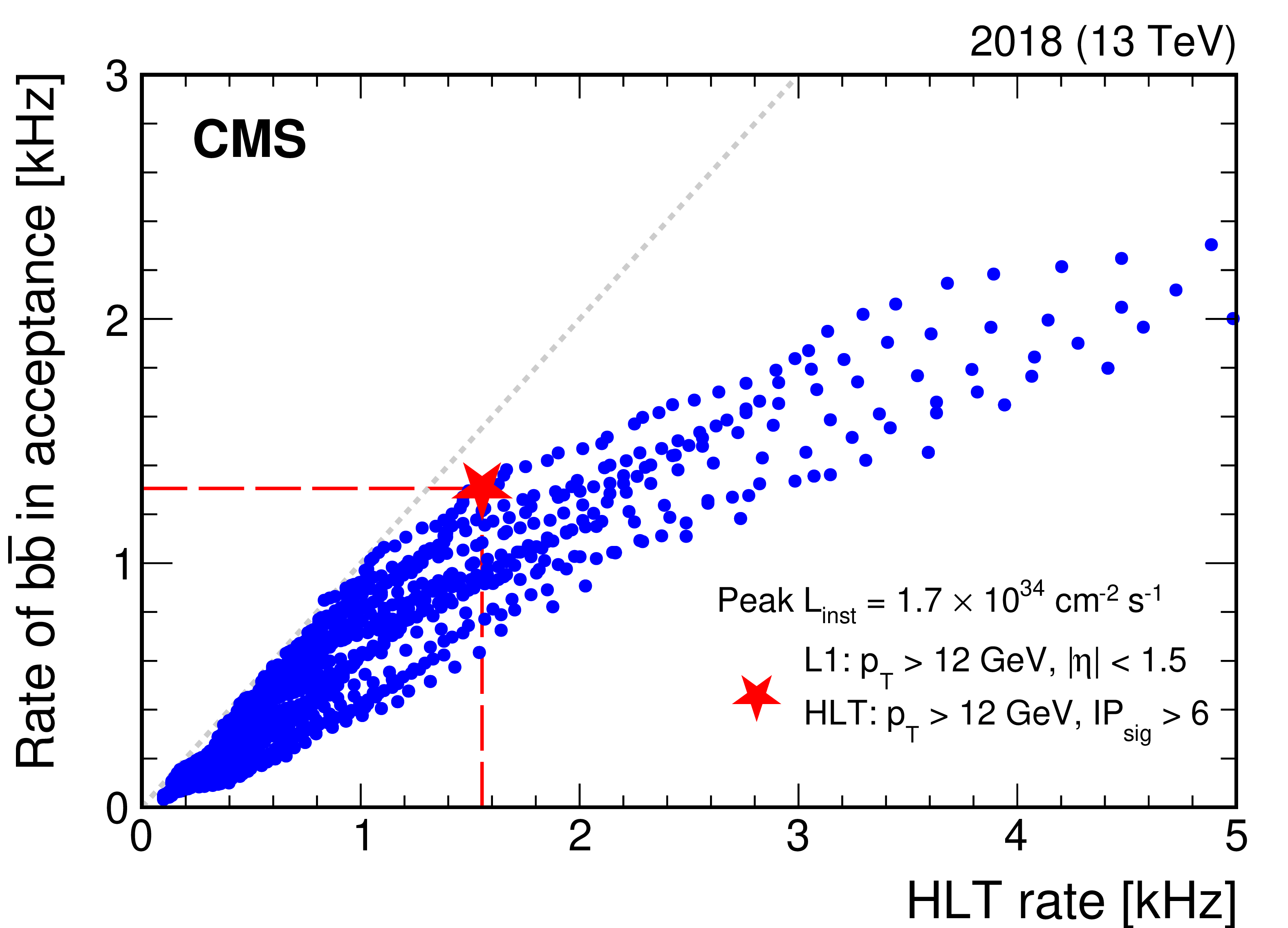
Left: an example scenario in which the $ {\mathrm{B}}\,\text{parking} $ data throughput per L1 trigger setting is adjusted to maintain an average of approximately 2\unitGB/s throughout an LHC fill. The dotted red and dashed blue lines trace the $ {\mathrm{B}}\,\text{parking} $ data throughput and maximum allowed HLT rate, respectively, determined for each trigger configuration. Changes in the trigger configuration are indicated by vertical green dashed lines. The trigger logic is adjusted to operate close to the permitted HLT rate. Right: rate of $ \mathrm{b} \overline{\mathrm{b}} $ events in acceptance versus HLT rate for a parameter scan over $ p_{\mathrm{T}} $ and $ \text{IP}_{\text{sig}} $ thresholds imposed in the HLT logic for the $ \mathcal{L}_{\text{inst}} $ and L1 requirements indicated in the legend; each point (blue circle) represents a unique pair of thresholds and the red star indicates the optimal pairing of $ {p_{\mathrm{T}}} > $ 12 GeV and $ {\text{IP}_{\text{sig}} > 6} $ at a peak $ {\mathcal{L}_{\text{inst}}} = $ 1.7 $\times$ 10$^{34}$ cm$^{-2}$s$^{-1}$ and an HLT rate close to the maximum allowed value of $ {\approx} $1.5 kHz. |
png pdf |
Figure 39-a:
Left: an example scenario in which the $ {\mathrm{B}}\,\text{parking} $ data throughput per L1 trigger setting is adjusted to maintain an average of approximately 2\unitGB/s throughout an LHC fill. The dotted red and dashed blue lines trace the $ {\mathrm{B}}\,\text{parking} $ data throughput and maximum allowed HLT rate, respectively, determined for each trigger configuration. Changes in the trigger configuration are indicated by vertical green dashed lines. The trigger logic is adjusted to operate close to the permitted HLT rate. Right: rate of $ \mathrm{b} \overline{\mathrm{b}} $ events in acceptance versus HLT rate for a parameter scan over $ p_{\mathrm{T}} $ and $ \text{IP}_{\text{sig}} $ thresholds imposed in the HLT logic for the $ \mathcal{L}_{\text{inst}} $ and L1 requirements indicated in the legend; each point (blue circle) represents a unique pair of thresholds and the red star indicates the optimal pairing of $ {p_{\mathrm{T}}} > $ 12 GeV and $ {\text{IP}_{\text{sig}} > 6} $ at a peak $ {\mathcal{L}_{\text{inst}}} = $ 1.7 $\times$ 10$^{34}$ cm$^{-2}$s$^{-1}$ and an HLT rate close to the maximum allowed value of $ {\approx} $1.5 kHz. |
png pdf |
Figure 39-b:
Left: an example scenario in which the $ {\mathrm{B}}\,\text{parking} $ data throughput per L1 trigger setting is adjusted to maintain an average of approximately 2\unitGB/s throughout an LHC fill. The dotted red and dashed blue lines trace the $ {\mathrm{B}}\,\text{parking} $ data throughput and maximum allowed HLT rate, respectively, determined for each trigger configuration. Changes in the trigger configuration are indicated by vertical green dashed lines. The trigger logic is adjusted to operate close to the permitted HLT rate. Right: rate of $ \mathrm{b} \overline{\mathrm{b}} $ events in acceptance versus HLT rate for a parameter scan over $ p_{\mathrm{T}} $ and $ \text{IP}_{\text{sig}} $ thresholds imposed in the HLT logic for the $ \mathcal{L}_{\text{inst}} $ and L1 requirements indicated in the legend; each point (blue circle) represents a unique pair of thresholds and the red star indicates the optimal pairing of $ {p_{\mathrm{T}}} > $ 12 GeV and $ {\text{IP}_{\text{sig}} > 6} $ at a peak $ {\mathcal{L}_{\text{inst}}} = $ 1.7 $\times$ 10$^{34}$ cm$^{-2}$s$^{-1}$ and an HLT rate close to the maximum allowed value of $ {\approx} $1.5 kHz. |
png pdf |
Figure 40:
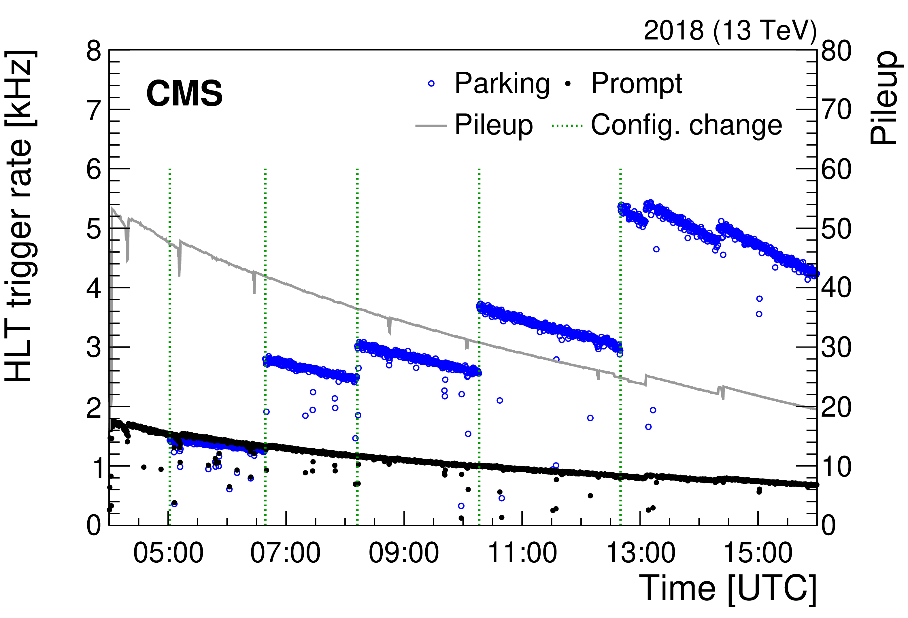
HLT trigger rates and the number of pileup events shown as a function of time during a representative LHC fill in 2018. The rates for the promptly reconstructed core physics (black solid markers) and $ {\mathrm{B}}\,\text{parking} $ (blue open markers) data streams are shown separately. Occasional lower rates are observed due to transient effects, such as the throttling of the trigger system in response to subdetector dead time [9]. Changes in the trigger configuration are indicated by vertical green dashed lines. |
png pdf |
Figure 41:
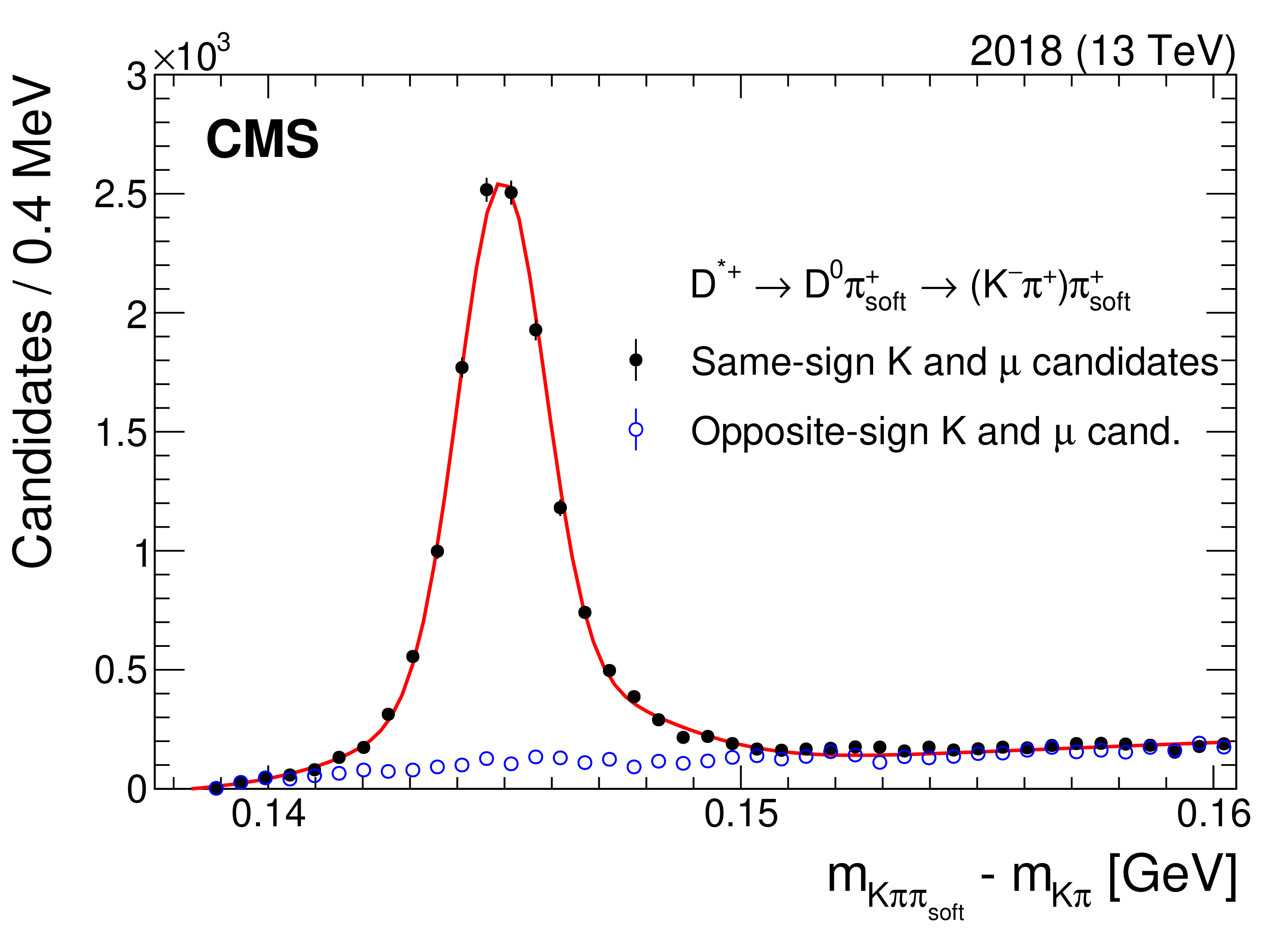
Mass difference between reconstructed $ \mathrm{D}^{*+} $ and $ \mathrm{D^0} $ candidates from the production mode $ {\mathrm{B}^0} \to \mathrm{D}^{*+} \mu^{-} \overline{\nu} $ and the subsequent decay chain $ \mathrm{D}^{*+} \to \mathrm{D^0}\pi^{+}_{\text{soft}} \to (\mathrm{K^-}\pi^{+})\pi^{+}_{\text{soft}} $. Events containing kaon and muon candidates with same-sign (opposite-sign) charges are indicated by solid (open) markers. |
png pdf |
Figure 42:
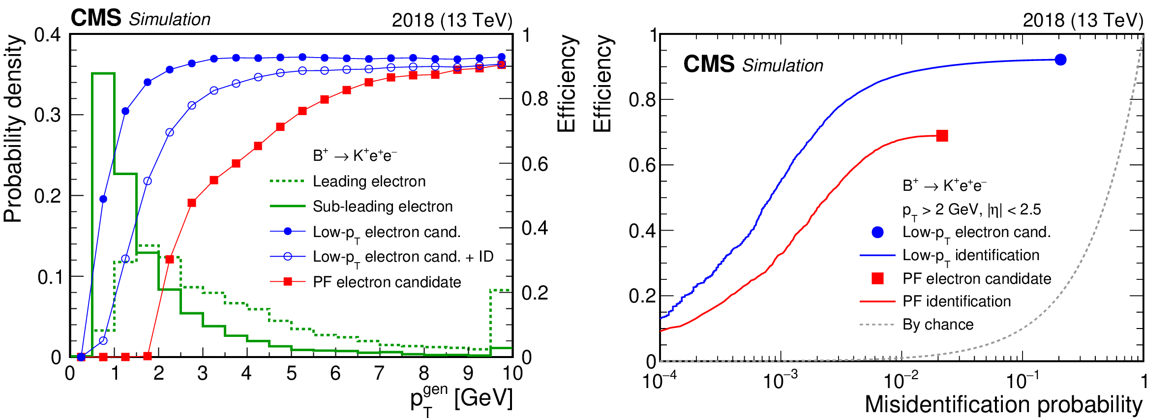
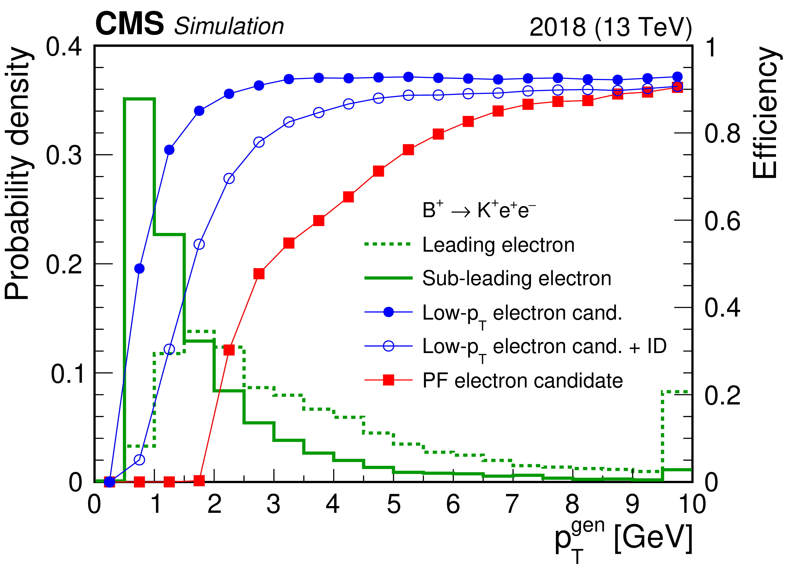
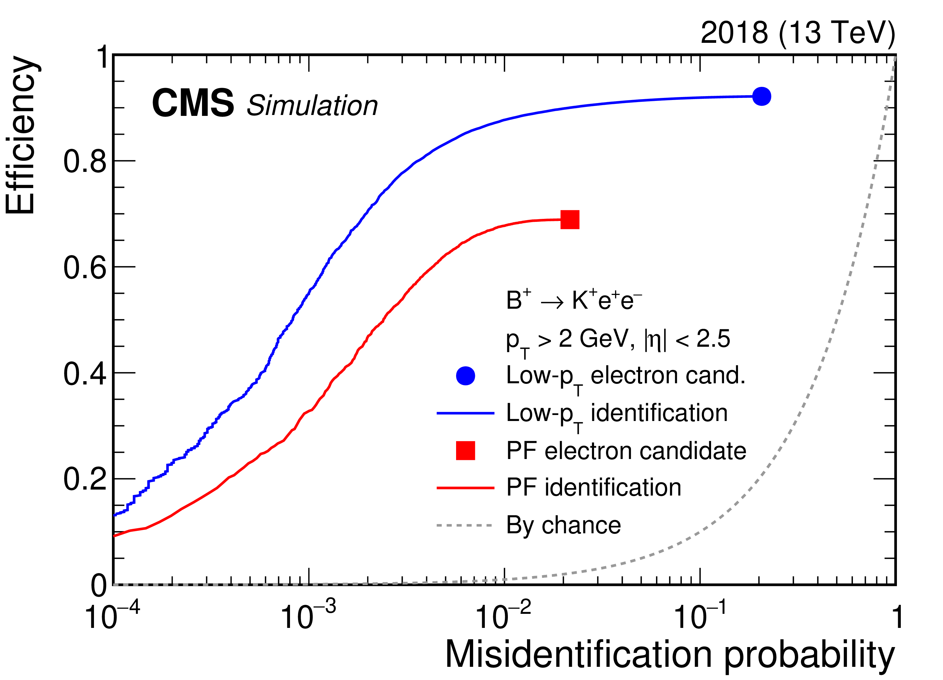
The left panel shows the $ p_{\mathrm{T}}^{\text{gen}} $ spectra of the leading and subleading electrons (dashed and solid green histograms) from $ {\mathrm{B}^{+}}\to\mathrm{K^+}\mathrm{e}^+\mathrm{e}^- $ decays, and the efficiency to identify genuine electrons as a function of $ p_{\mathrm{T}}^{\text{gen}} $ for PF (solid red squares) and low-$ p_{\mathrm{T}} $ electron candidates (solid blue circles). Efficiencies for the low-$ p_{\mathrm{T}} $ electron candidates that satisfy an ID score threshold, tuned to give the same misidentification probability as for PF electron candidates, are also shown (open markers). The right panel shows the performance of the PF (solid red square) and low-$ p_{\mathrm{T}} $ (solid blue circle) reconstruction algorithms and their corresponding ID algorithms (curves). The efficiencies and misidentification probabilities are determined relative to charged-particle tracks obtained from simulation, for both $ {\mathrm{B}^{+}}\to\mathrm{K^+}\mathrm{e}^+\mathrm{e}^- $ decays and background processes, and satisfying $ {p_{\mathrm{T}}} > $ 2 GeV and $ |\eta| < $ 2.5. |
png pdf |
Figure 42-a:
The left panel shows the $ p_{\mathrm{T}}^{\text{gen}} $ spectra of the leading and subleading electrons (dashed and solid green histograms) from $ {\mathrm{B}^{+}}\to\mathrm{K^+}\mathrm{e}^+\mathrm{e}^- $ decays, and the efficiency to identify genuine electrons as a function of $ p_{\mathrm{T}}^{\text{gen}} $ for PF (solid red squares) and low-$ p_{\mathrm{T}} $ electron candidates (solid blue circles). Efficiencies for the low-$ p_{\mathrm{T}} $ electron candidates that satisfy an ID score threshold, tuned to give the same misidentification probability as for PF electron candidates, are also shown (open markers). The right panel shows the performance of the PF (solid red square) and low-$ p_{\mathrm{T}} $ (solid blue circle) reconstruction algorithms and their corresponding ID algorithms (curves). The efficiencies and misidentification probabilities are determined relative to charged-particle tracks obtained from simulation, for both $ {\mathrm{B}^{+}}\to\mathrm{K^+}\mathrm{e}^+\mathrm{e}^- $ decays and background processes, and satisfying $ {p_{\mathrm{T}}} > $ 2 GeV and $ |\eta| < $ 2.5. |
png pdf |
Figure 42-b:
The left panel shows the $ p_{\mathrm{T}}^{\text{gen}} $ spectra of the leading and subleading electrons (dashed and solid green histograms) from $ {\mathrm{B}^{+}}\to\mathrm{K^+}\mathrm{e}^+\mathrm{e}^- $ decays, and the efficiency to identify genuine electrons as a function of $ p_{\mathrm{T}}^{\text{gen}} $ for PF (solid red squares) and low-$ p_{\mathrm{T}} $ electron candidates (solid blue circles). Efficiencies for the low-$ p_{\mathrm{T}} $ electron candidates that satisfy an ID score threshold, tuned to give the same misidentification probability as for PF electron candidates, are also shown (open markers). The right panel shows the performance of the PF (solid red square) and low-$ p_{\mathrm{T}} $ (solid blue circle) reconstruction algorithms and their corresponding ID algorithms (curves). The efficiencies and misidentification probabilities are determined relative to charged-particle tracks obtained from simulation, for both $ {\mathrm{B}^{+}}\to\mathrm{K^+}\mathrm{e}^+\mathrm{e}^- $ decays and background processes, and satisfying $ {p_{\mathrm{T}}} > $ 2 GeV and $ |\eta| < $ 2.5. |

png pdf |
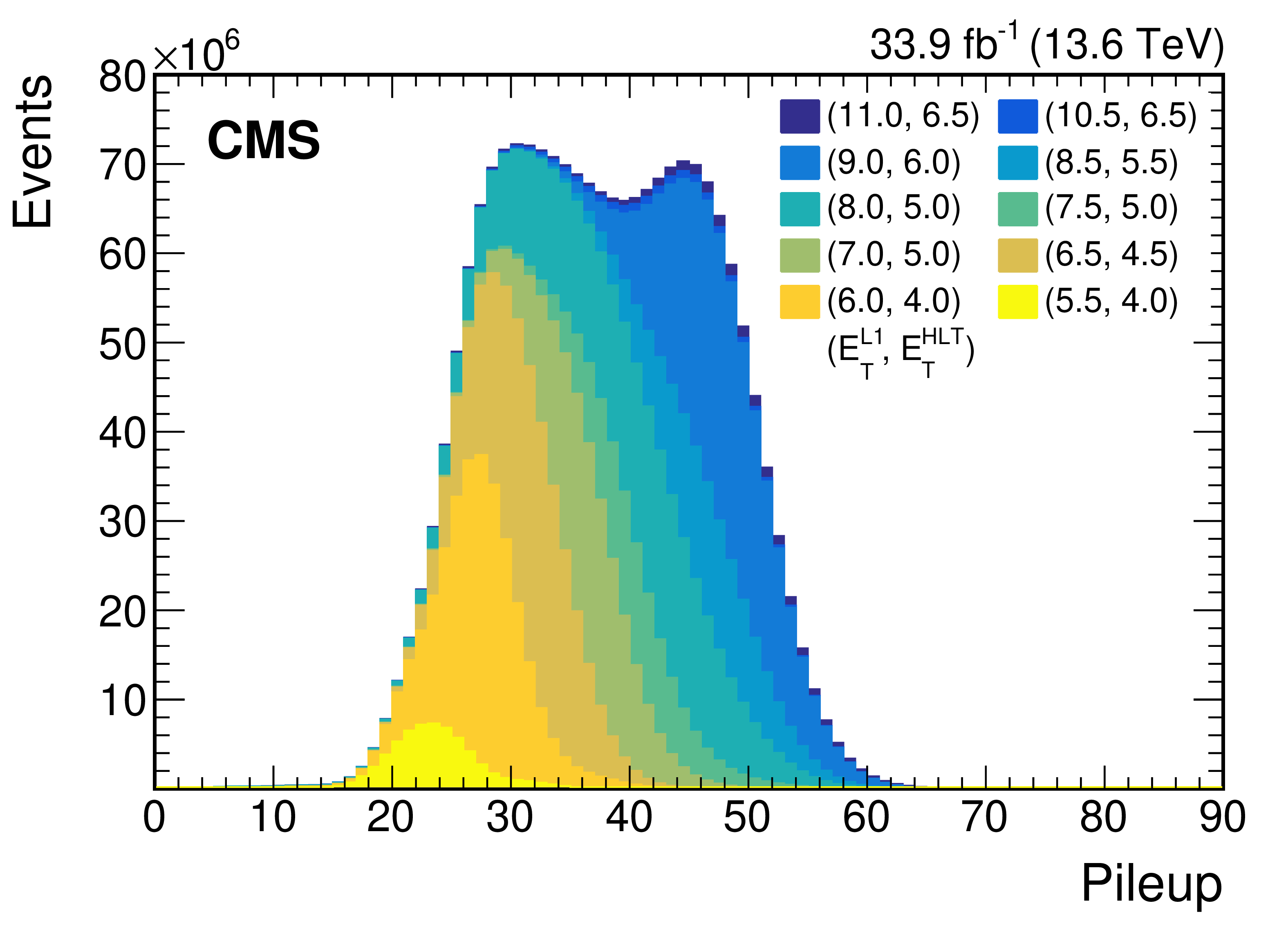
Figure 43:
The pileup distribution obtained from the $ {\mathrm{B}}\,\text{parking} $ data set. Contributions from each trigger combination are shown, with the histogram areas normalized to the number of events recorded by each trigger. |
png pdf |
Figure 44:
The invariant mass distribution for pairs of oppositely charged muons originating from a common vertex, obtained from a subset of the $ {\mathrm{B}}\,\text{parking} $ data. |
png pdf |
Figure 45:
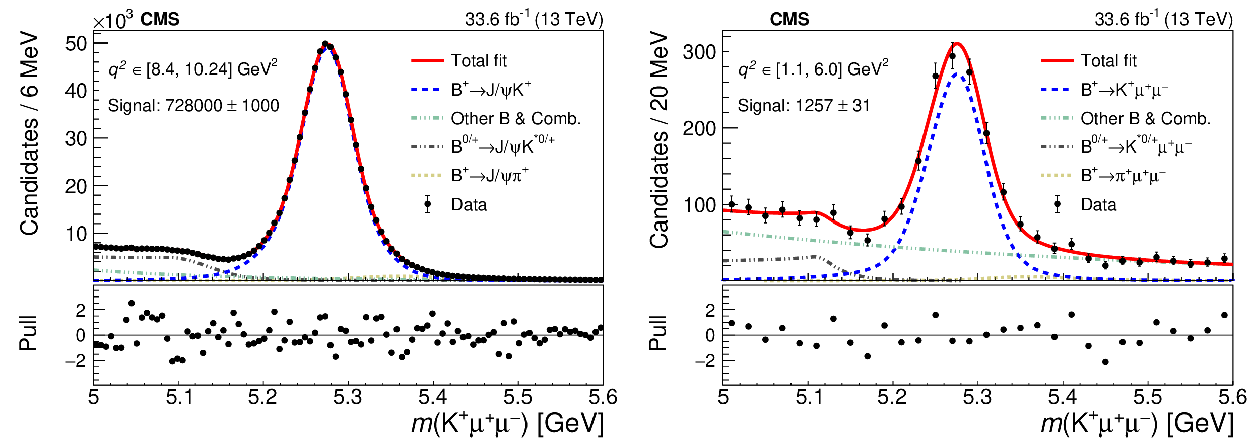
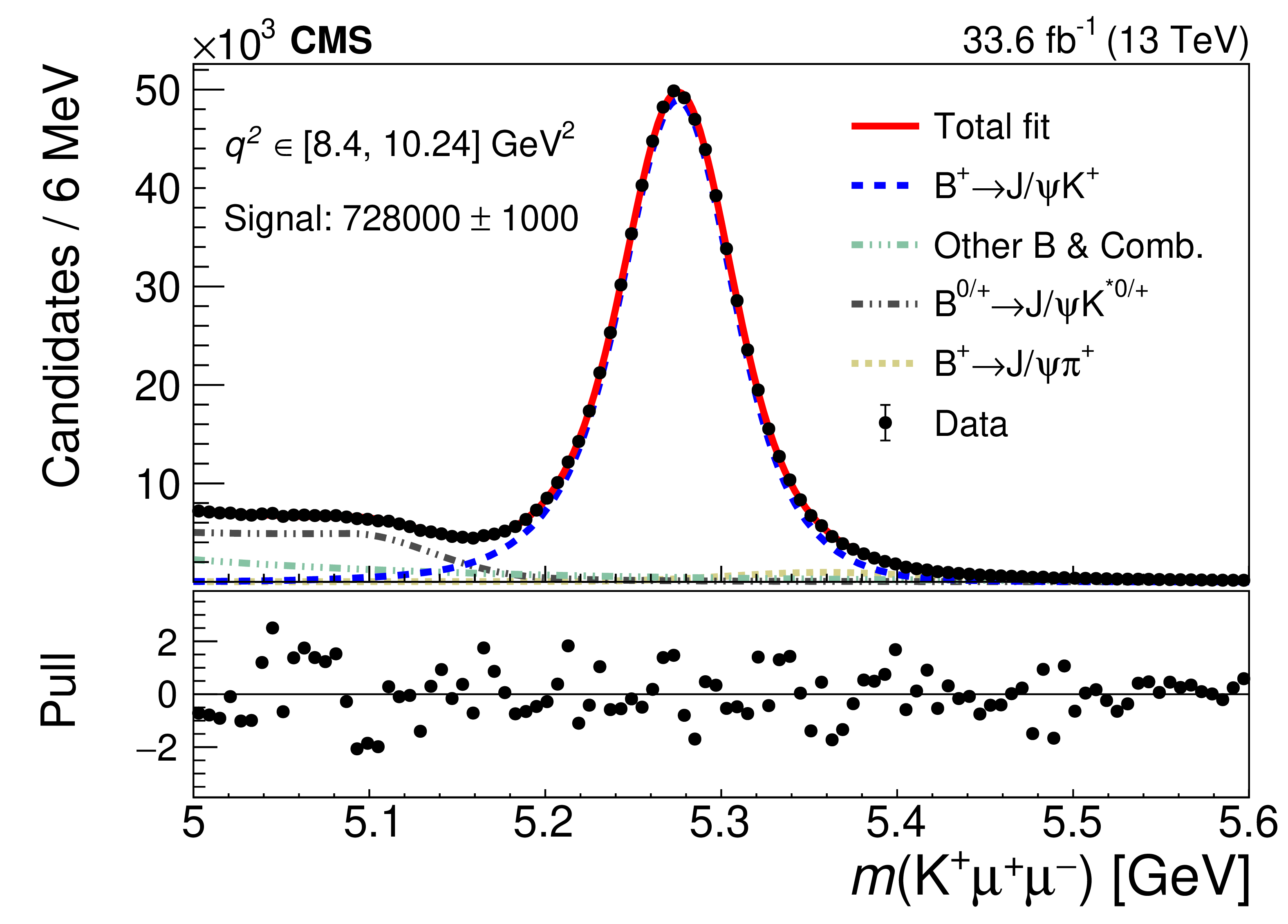
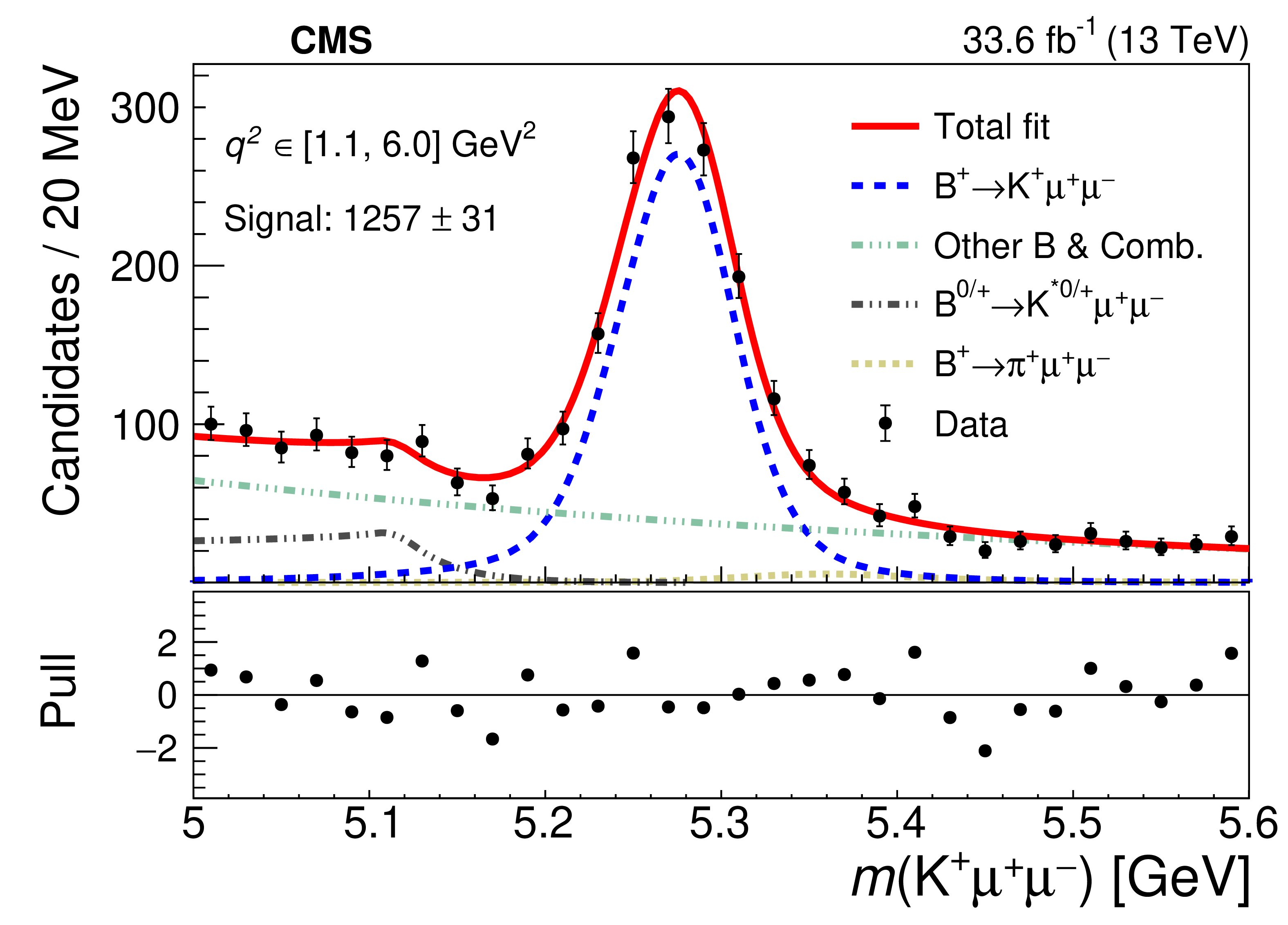
Results of an unbinned likelihood fit to the invariant mass distributions for the the $ {\mathrm{B}^{+}}\to{\mathrm{J}/\psi} (\to\mu^{+}\mu^{-})\mathrm{K^+} $ (left) and the $ {\mathrm{B}^{+}}\to\mathrm{K^+}\mu^{+}\mu^{-} $ (right) channels. Various functions are used to parametrize the contributions from the signal and various background processes. Taken from Ref. [152]. |
png pdf |
Figure 45-a:
Results of an unbinned likelihood fit to the invariant mass distributions for the the $ {\mathrm{B}^{+}}\to{\mathrm{J}/\psi} (\to\mu^{+}\mu^{-})\mathrm{K^+} $ (left) and the $ {\mathrm{B}^{+}}\to\mathrm{K^+}\mu^{+}\mu^{-} $ (right) channels. Various functions are used to parametrize the contributions from the signal and various background processes. Taken from Ref. [152]. |
png pdf |
Figure 45-b:
Results of an unbinned likelihood fit to the invariant mass distributions for the the $ {\mathrm{B}^{+}}\to{\mathrm{J}/\psi} (\to\mu^{+}\mu^{-})\mathrm{K^+} $ (left) and the $ {\mathrm{B}^{+}}\to\mathrm{K^+}\mu^{+}\mu^{-} $ (right) channels. Various functions are used to parametrize the contributions from the signal and various background processes. Taken from Ref. [152]. |
png pdf |
Figure 46:
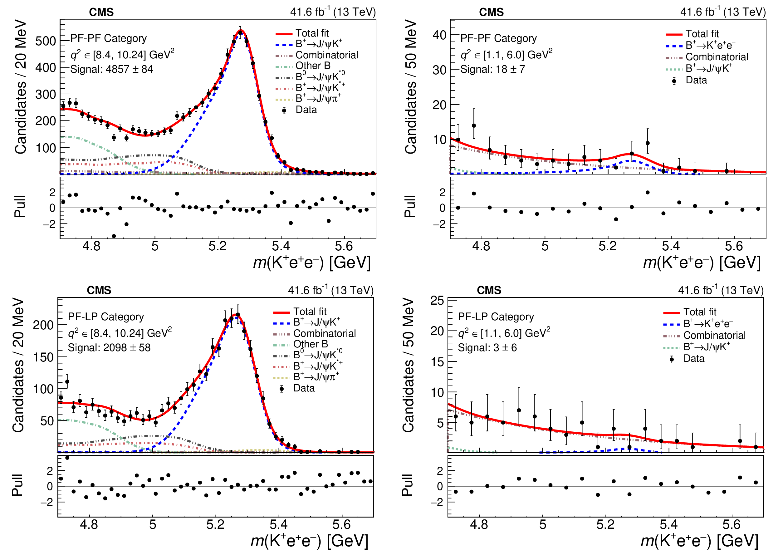
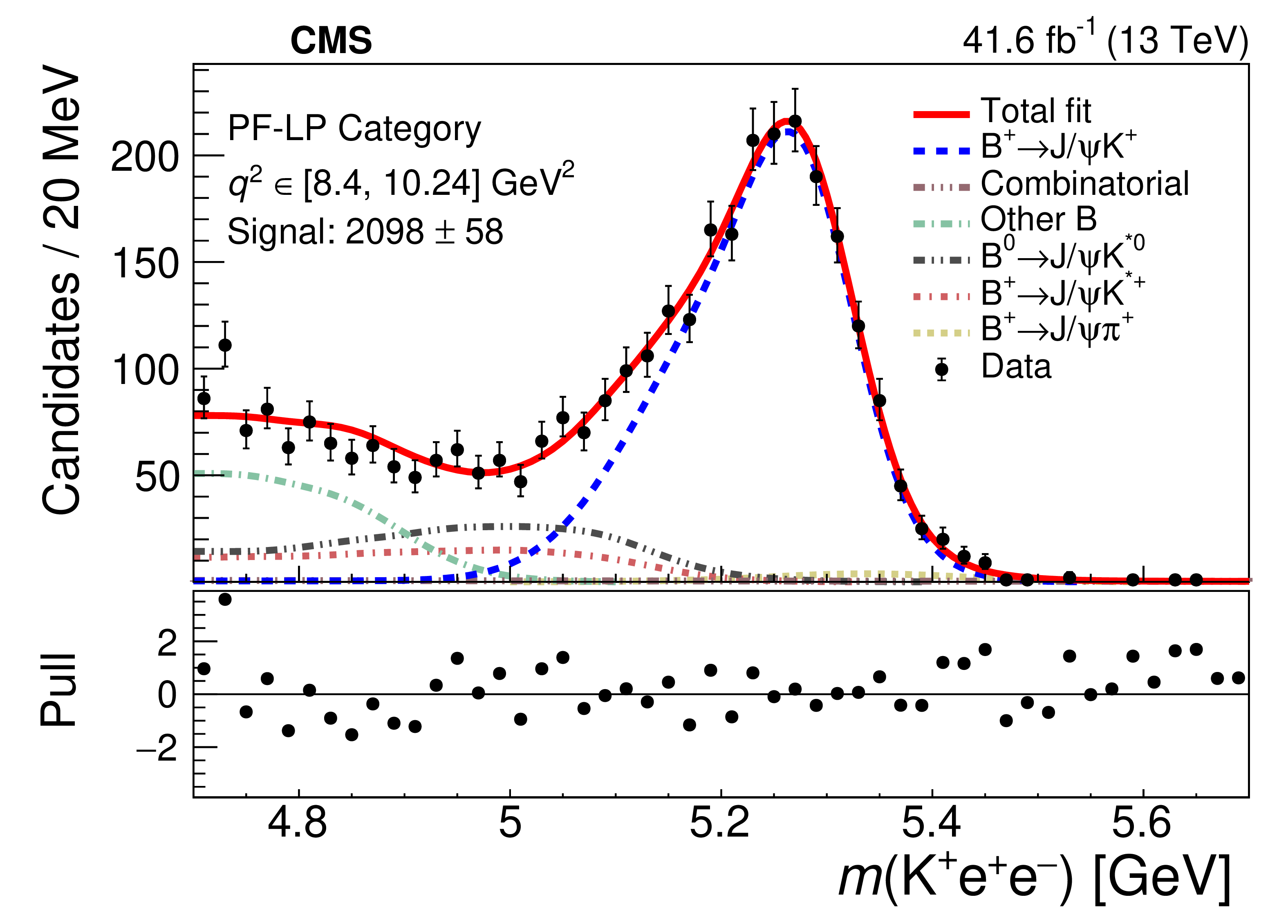
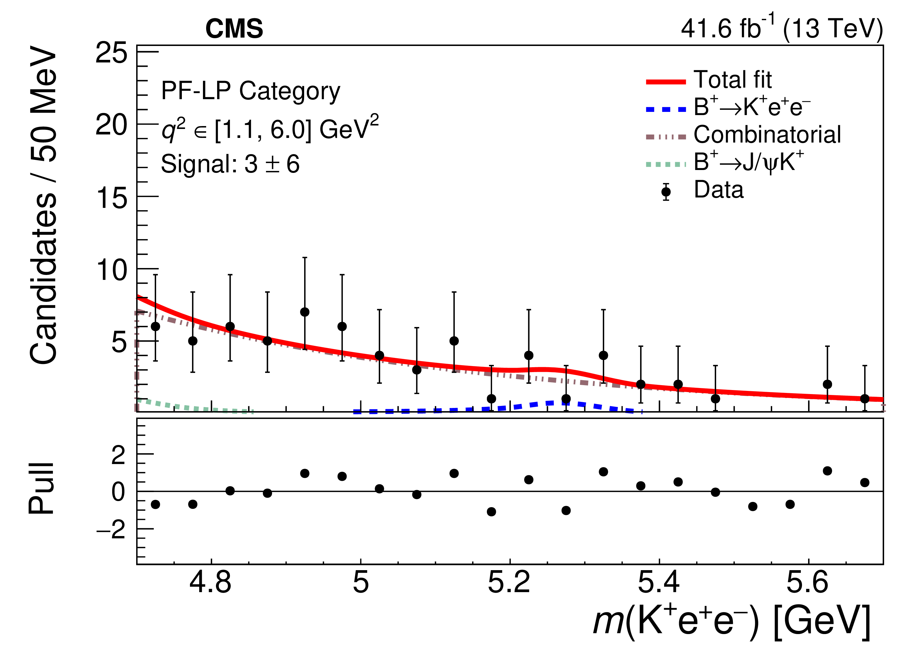
Results of an unbinned likelihood fit to the invariant mass distributions for the $ {\mathrm{B}^{+}}\to{\mathrm{J}/\psi} (\to\mathrm{e}^+\mathrm{e}^-)\mathrm{K^+} $ (left) and the $ {\mathrm{B}^{+}}\to\mathrm{K^+}\mathrm{e}^+\mathrm{e}^- $ (right) channels. The upper (lower) panels are for candidates using the PF-PF (PF-LP) category. Various functions are used to parametrize the contributions from the signal and various background processes. Taken from Ref. [152]. |

png pdf |
Figure 46-a:
Results of an unbinned likelihood fit to the invariant mass distributions for the $ {\mathrm{B}^{+}}\to{\mathrm{J}/\psi} (\to\mathrm{e}^+\mathrm{e}^-)\mathrm{K^+} $ (left) and the $ {\mathrm{B}^{+}}\to\mathrm{K^+}\mathrm{e}^+\mathrm{e}^- $ (right) channels. The upper (lower) panels are for candidates using the PF-PF (PF-LP) category. Various functions are used to parametrize the contributions from the signal and various background processes. Taken from Ref. [152]. |

png pdf |
Figure 46-b:
Results of an unbinned likelihood fit to the invariant mass distributions for the $ {\mathrm{B}^{+}}\to{\mathrm{J}/\psi} (\to\mathrm{e}^+\mathrm{e}^-)\mathrm{K^+} $ (left) and the $ {\mathrm{B}^{+}}\to\mathrm{K^+}\mathrm{e}^+\mathrm{e}^- $ (right) channels. The upper (lower) panels are for candidates using the PF-PF (PF-LP) category. Various functions are used to parametrize the contributions from the signal and various background processes. Taken from Ref. [152]. |
png pdf |
Figure 46-c:
Results of an unbinned likelihood fit to the invariant mass distributions for the $ {\mathrm{B}^{+}}\to{\mathrm{J}/\psi} (\to\mathrm{e}^+\mathrm{e}^-)\mathrm{K^+} $ (left) and the $ {\mathrm{B}^{+}}\to\mathrm{K^+}\mathrm{e}^+\mathrm{e}^- $ (right) channels. The upper (lower) panels are for candidates using the PF-PF (PF-LP) category. Various functions are used to parametrize the contributions from the signal and various background processes. Taken from Ref. [152]. |
png pdf |
Figure 46-d:
Results of an unbinned likelihood fit to the invariant mass distributions for the $ {\mathrm{B}^{+}}\to{\mathrm{J}/\psi} (\to\mathrm{e}^+\mathrm{e}^-)\mathrm{K^+} $ (left) and the $ {\mathrm{B}^{+}}\to\mathrm{K^+}\mathrm{e}^+\mathrm{e}^- $ (right) channels. The upper (lower) panels are for candidates using the PF-PF (PF-LP) category. Various functions are used to parametrize the contributions from the signal and various background processes. Taken from Ref. [152]. |
png pdf |
Figure 47:
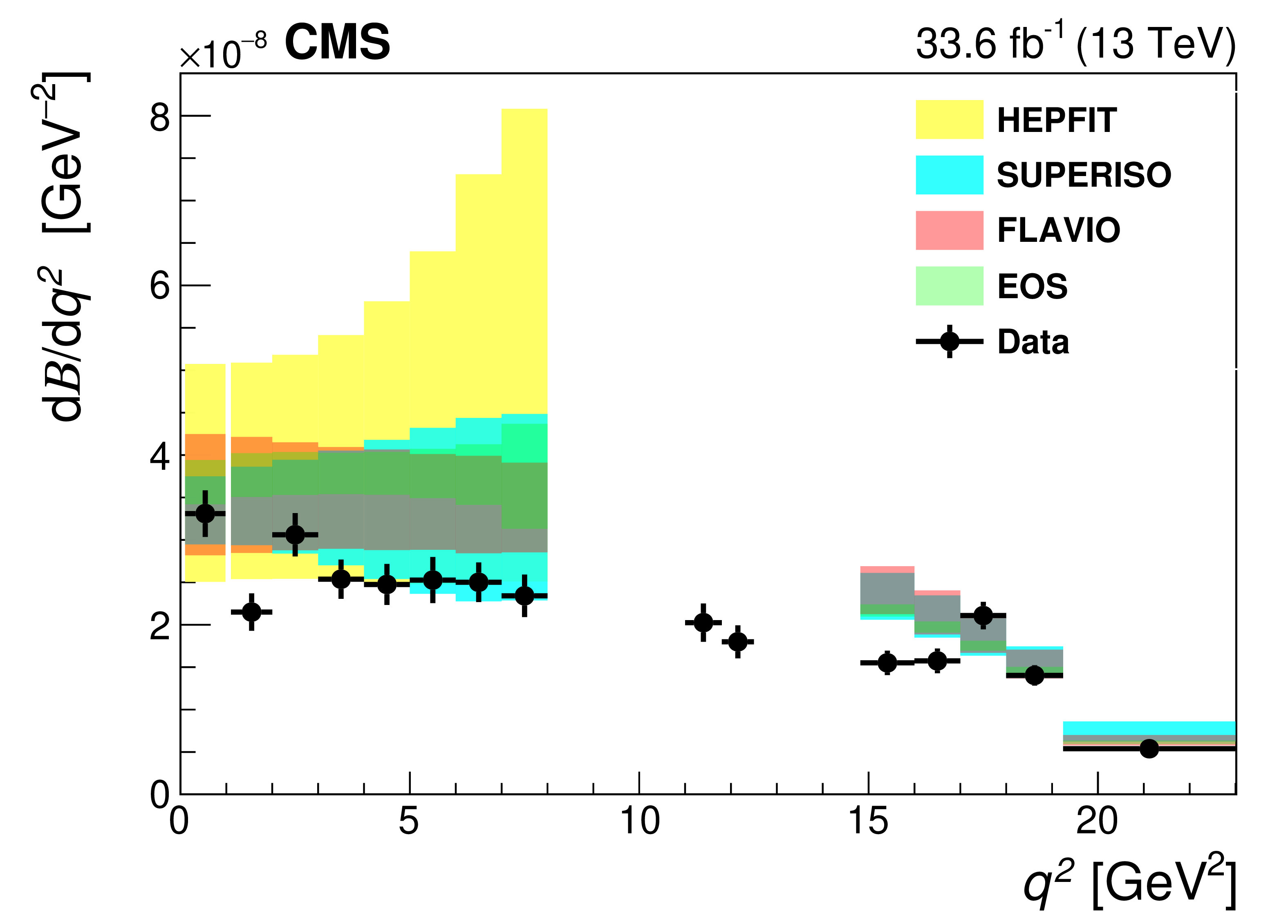
Comparison of the measured differential $ {\mathrm{B}^{+}}\to\mathrm{K^+}\mu^{+}\mu^{-} $ branching fraction with the theoretical predictions obtained using HEPFIT, SUPERISO, FLAVIO, and EOS packages. Reliable predictions are not available between the $ \mathrm{J}/\psi $ and \PGyP2S resonance regions. The HEPFIT predictions are available only for $ q^2 < $ 8 GeV$^{2} $. Taken from Ref. [152]. |
png pdf |
Figure 48:
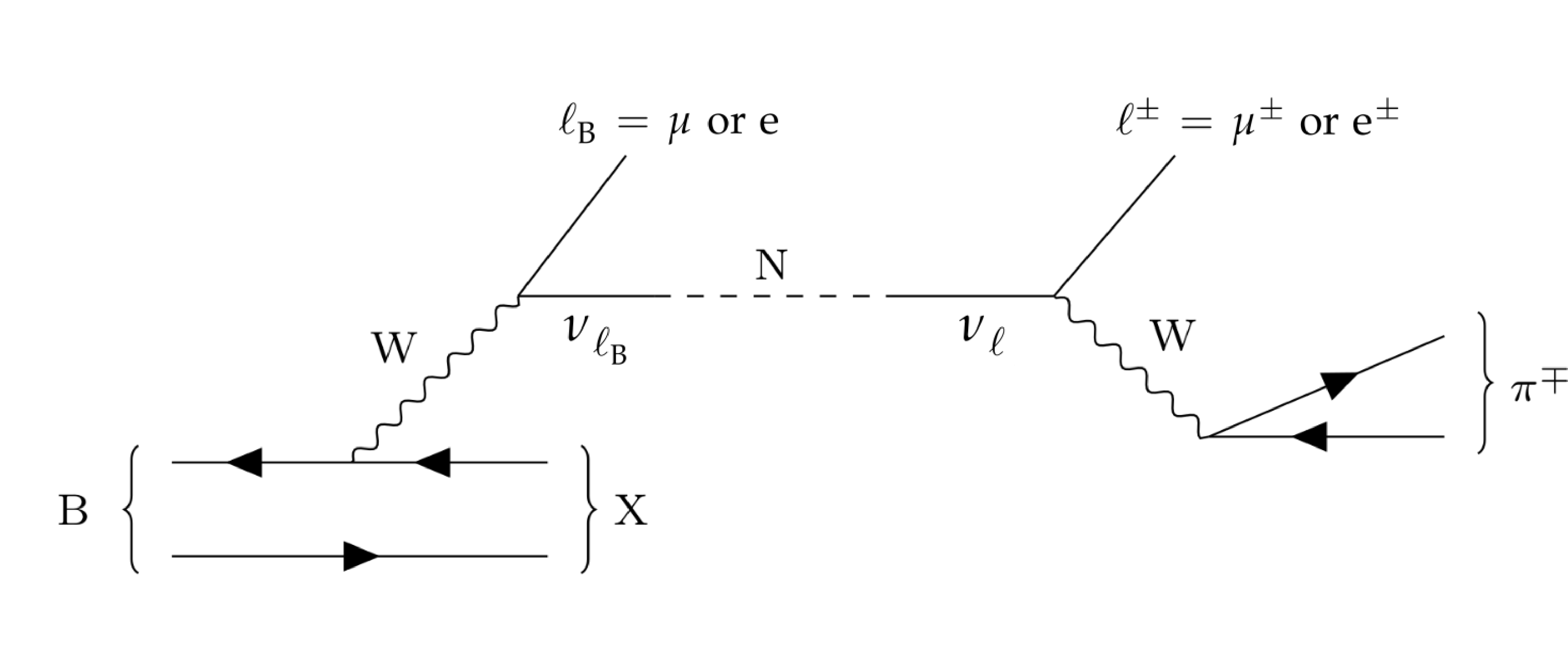
Feynman diagram of a semileptonic decay of a $ {\mathrm{B}} $ meson into the primary lepton ($ \ell_{P} $), a hadronic system (X), and a SM neutrino, which then mixes with a heavy neutrino ($ \mathrm{N} $). The $ \mathrm{N} $ decays weakly into a charged lepton $ \ell^\pm $ and a charged pion $ \pi^{\mp} $, forming a vertex displaced from the $ {\mathrm{p}}{\mathrm{p}} $ interaction point. Taken from Ref. [158]. |
png pdf |
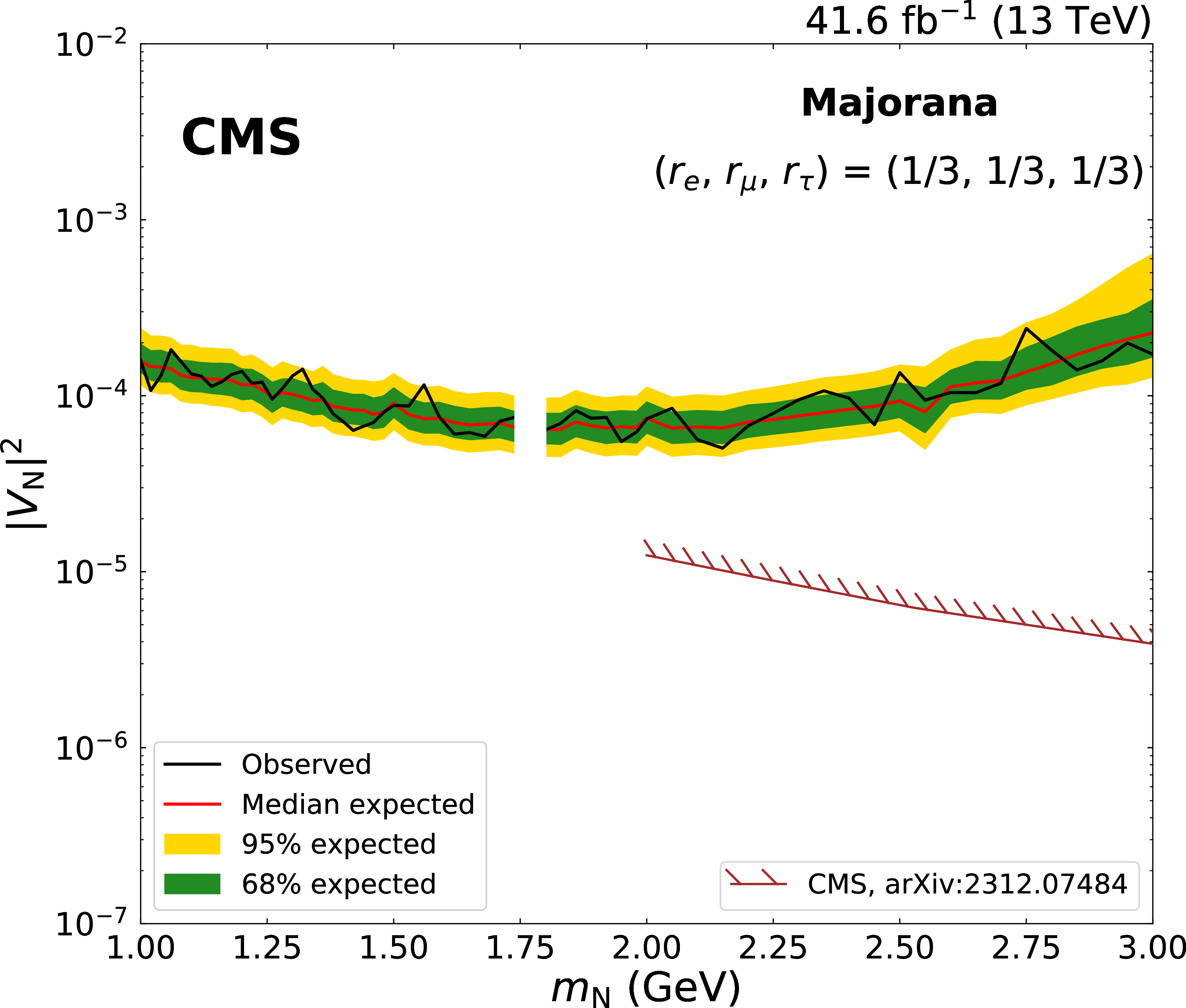
Figure 49:
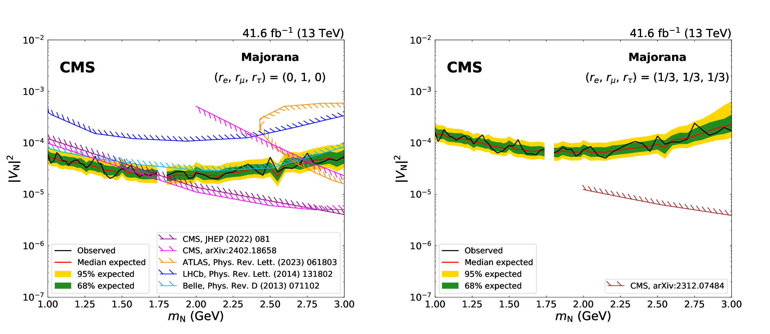
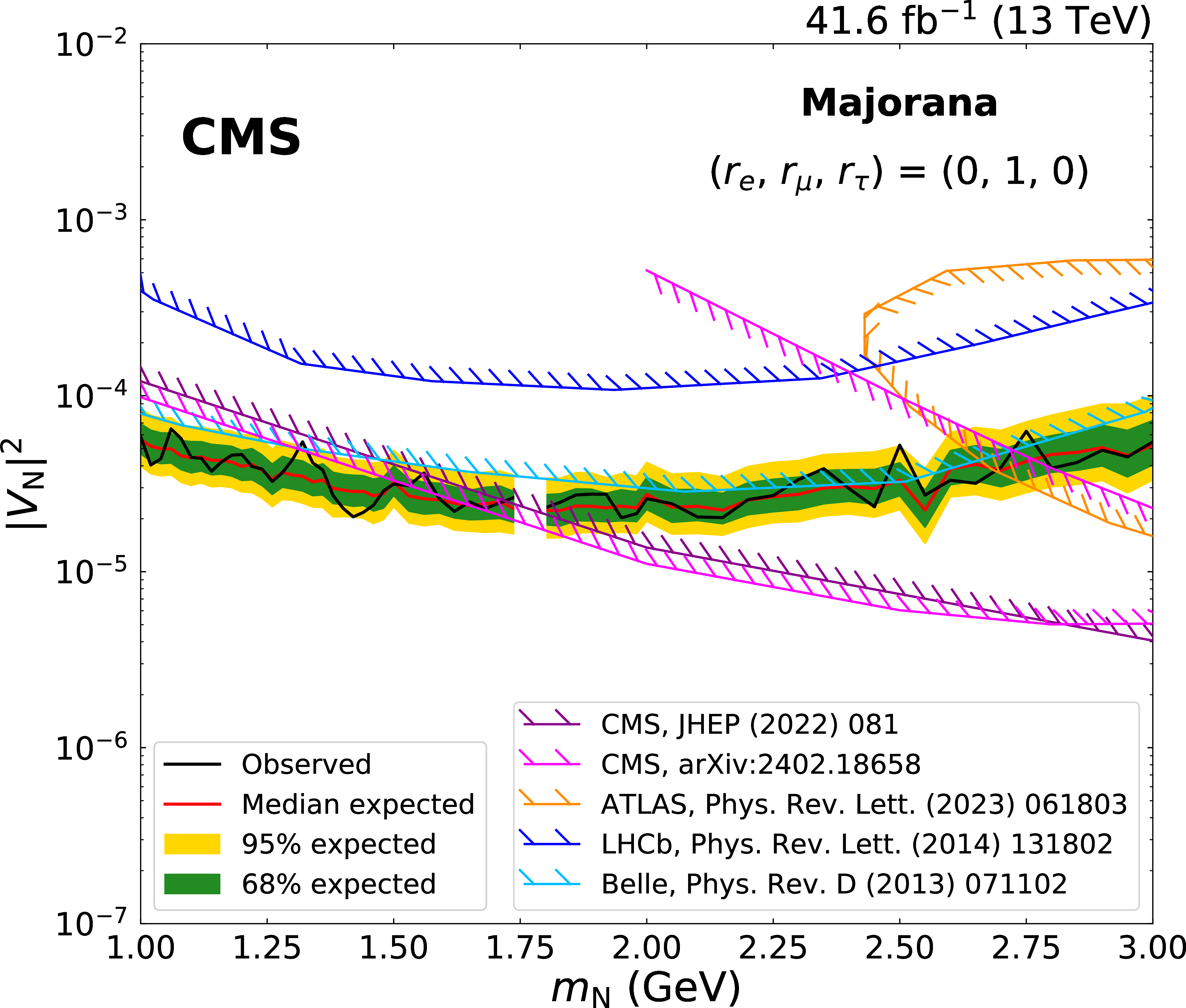
Expected and observed 95% CL limits on $ |V_{\mathrm{N}}|^2 $ as a function of $ m_\mathrm{N} $ in the Majorana scenario, for the coupling hypotheses ($ r_\mathrm{e} $, $ r_\mu $, $ r_\tau $) = (0, 1, 0) on the left and ($ r_\mathrm{e} $, $ r_\mu $, $ r_\tau $) = (1/3, 1/3, 1/3) on the right. The mass range with no limits shown corresponds to the $ \mathrm{D^0} $ meson veto employed by the search. Taken from Ref. [158]. |
png pdf |
Figure 49-a:
Expected and observed 95% CL limits on $ |V_{\mathrm{N}}|^2 $ as a function of $ m_\mathrm{N} $ in the Majorana scenario, for the coupling hypotheses ($ r_\mathrm{e} $, $ r_\mu $, $ r_\tau $) = (0, 1, 0) on the left and ($ r_\mathrm{e} $, $ r_\mu $, $ r_\tau $) = (1/3, 1/3, 1/3) on the right. The mass range with no limits shown corresponds to the $ \mathrm{D^0} $ meson veto employed by the search. Taken from Ref. [158]. |
png pdf |
Figure 49-b:
Expected and observed 95% CL limits on $ |V_{\mathrm{N}}|^2 $ as a function of $ m_\mathrm{N} $ in the Majorana scenario, for the coupling hypotheses ($ r_\mathrm{e} $, $ r_\mu $, $ r_\tau $) = (0, 1, 0) on the left and ($ r_\mathrm{e} $, $ r_\mu $, $ r_\tau $) = (1/3, 1/3, 1/3) on the right. The mass range with no limits shown corresponds to the $ \mathrm{D^0} $ meson veto employed by the search. Taken from Ref. [158]. |
png pdf |
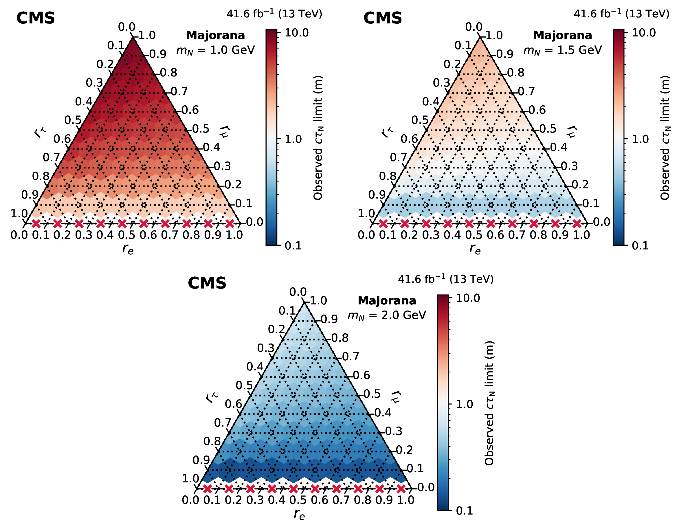
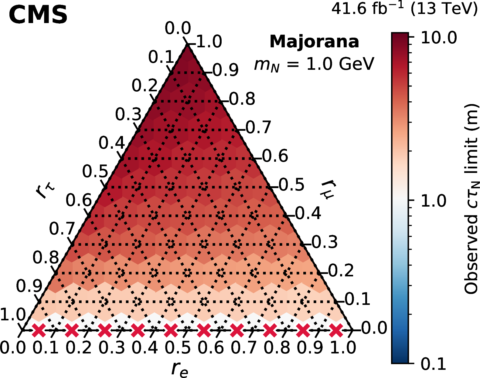
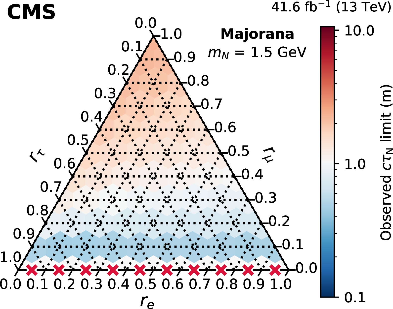
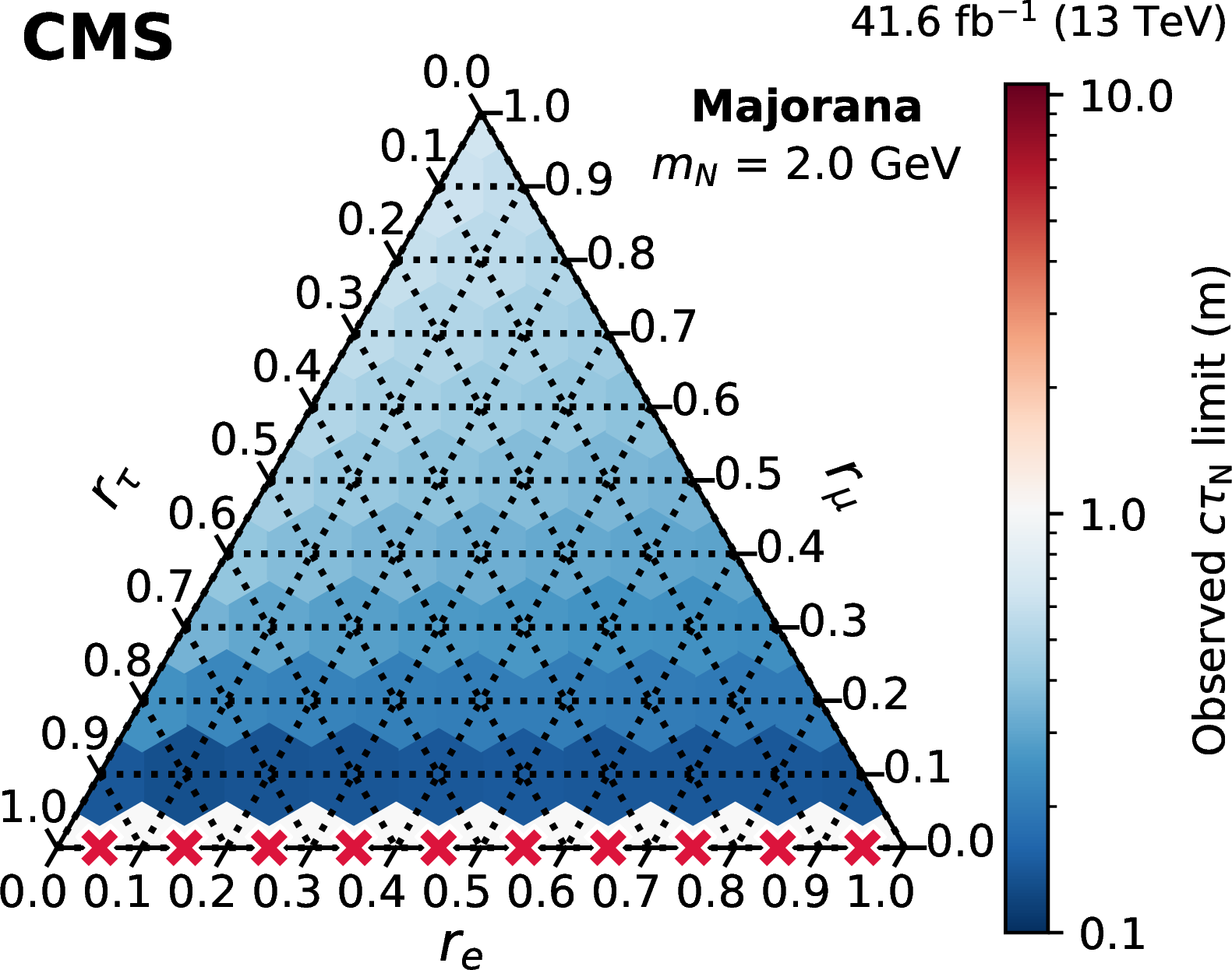
Figure 50:
Observed limits on $ c\tau_{\mathrm{N}} $ as a function of the coupling ratios ($ r_\mathrm{e} $, $ r_\mu $, $ r_\tau $) for fixed $ \mathrm{N} $ masses of 1 GeV (upper left), 1.5 GeV (upper right), and 2 GeV (lower center), in the Majorana scenario. A red cross indicates that no exclusion limit was set for that point. The tick orientation indicates the direction of reading. Taken from Ref. [158]. |
png pdf |
Figure 50-a:
Observed limits on $ c\tau_{\mathrm{N}} $ as a function of the coupling ratios ($ r_\mathrm{e} $, $ r_\mu $, $ r_\tau $) for fixed $ \mathrm{N} $ masses of 1 GeV (upper left), 1.5 GeV (upper right), and 2 GeV (lower center), in the Majorana scenario. A red cross indicates that no exclusion limit was set for that point. The tick orientation indicates the direction of reading. Taken from Ref. [158]. |
png pdf |
Figure 50-b:
Observed limits on $ c\tau_{\mathrm{N}} $ as a function of the coupling ratios ($ r_\mathrm{e} $, $ r_\mu $, $ r_\tau $) for fixed $ \mathrm{N} $ masses of 1 GeV (upper left), 1.5 GeV (upper right), and 2 GeV (lower center), in the Majorana scenario. A red cross indicates that no exclusion limit was set for that point. The tick orientation indicates the direction of reading. Taken from Ref. [158]. |
png pdf |
Figure 50-c:
Observed limits on $ c\tau_{\mathrm{N}} $ as a function of the coupling ratios ($ r_\mathrm{e} $, $ r_\mu $, $ r_\tau $) for fixed $ \mathrm{N} $ masses of 1 GeV (upper left), 1.5 GeV (upper right), and 2 GeV (lower center), in the Majorana scenario. A red cross indicates that no exclusion limit was set for that point. The tick orientation indicates the direction of reading. Taken from Ref. [158]. |
png pdf |
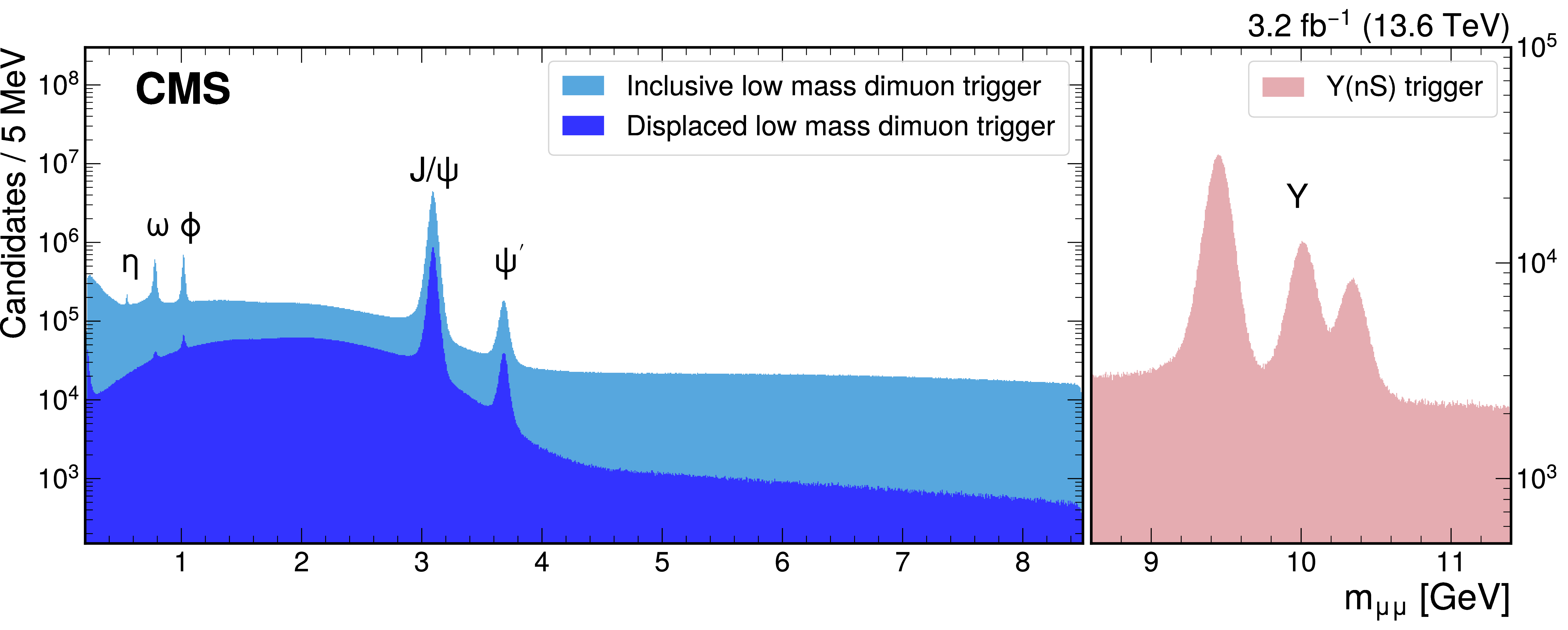
Figure 51:
Dimuon mass spectra obtained from data recorded in 2022 during Run 3, corresponding to $ {\mathcal{L}_{\text{int}}} = $ 3.2 fb$^{-1}$. In the range $ {2m_{\mu}^{\text{PDG}}} < m_{\mu\mu} < $ 8.5 GeV, the light blue distribution represents the subset of dimuon events triggered by the inclusive low-mass trigger algorithm, while the dark blue distribution shows the subset of dimuon events triggered by the displaced low-mass trigger path. In the range 8.5 $ < m_{\mu\mu} < $ 11.5 GeV, dimuon events are instead triggered by the HLT paths targeting the $ \Upsilon{\textrm{(nS)}} $ resonances, which are shown by the pink distribution. |
png pdf |
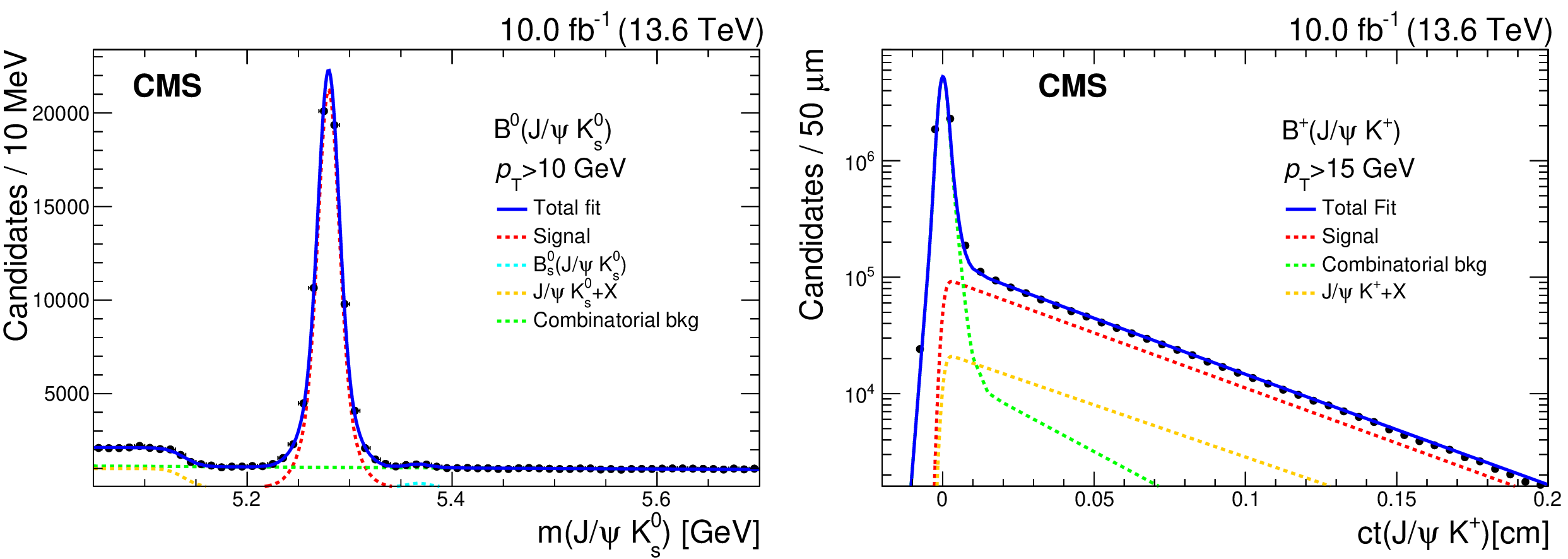
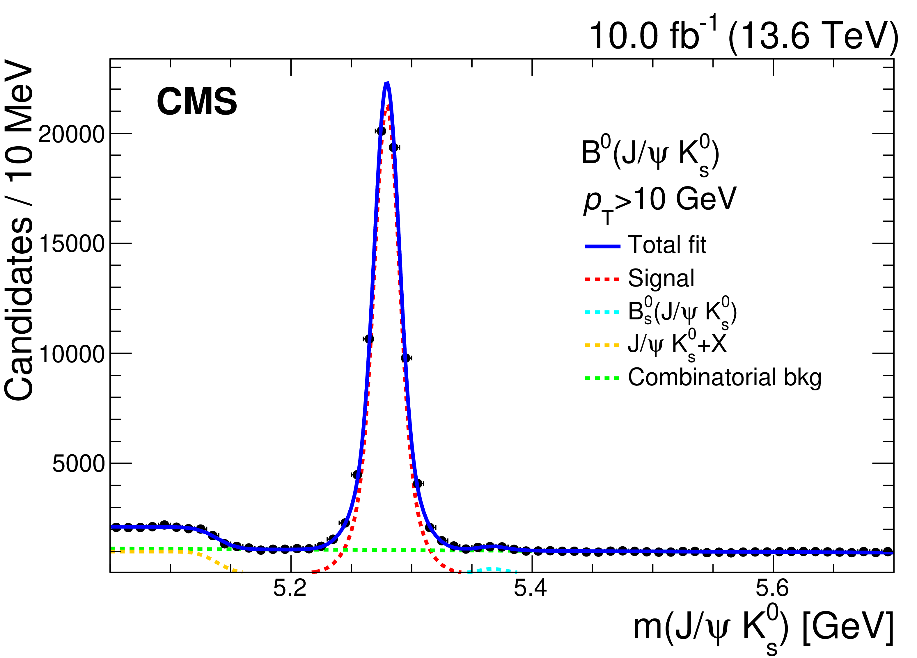
Figure 52:
Left: invariant mass distribution for candidate $ {\mathrm{B}^0}\to\mathrm{J}/\psi\mathrm{K^0_S} $ decays. Right: proper decay length (ct) distribution obtained from candidate $ {\mathrm{B}^{+}}\to{\mathrm{J}/\psi} (\to\mu^{+}\mu^{-})\mathrm{K^+} $ decays. Both types of candidates are reconstructed from events recorded using the dimuon triggers. |
png pdf |
Figure 52-a:
Left: invariant mass distribution for candidate $ {\mathrm{B}^0}\to\mathrm{J}/\psi\mathrm{K^0_S} $ decays. Right: proper decay length (ct) distribution obtained from candidate $ {\mathrm{B}^{+}}\to{\mathrm{J}/\psi} (\to\mu^{+}\mu^{-})\mathrm{K^+} $ decays. Both types of candidates are reconstructed from events recorded using the dimuon triggers. |

png pdf |
Figure 52-b:
Left: invariant mass distribution for candidate $ {\mathrm{B}^0}\to\mathrm{J}/\psi\mathrm{K^0_S} $ decays. Right: proper decay length (ct) distribution obtained from candidate $ {\mathrm{B}^{+}}\to{\mathrm{J}/\psi} (\to\mu^{+}\mu^{-})\mathrm{K^+} $ decays. Both types of candidates are reconstructed from events recorded using the dimuon triggers. |
png pdf |
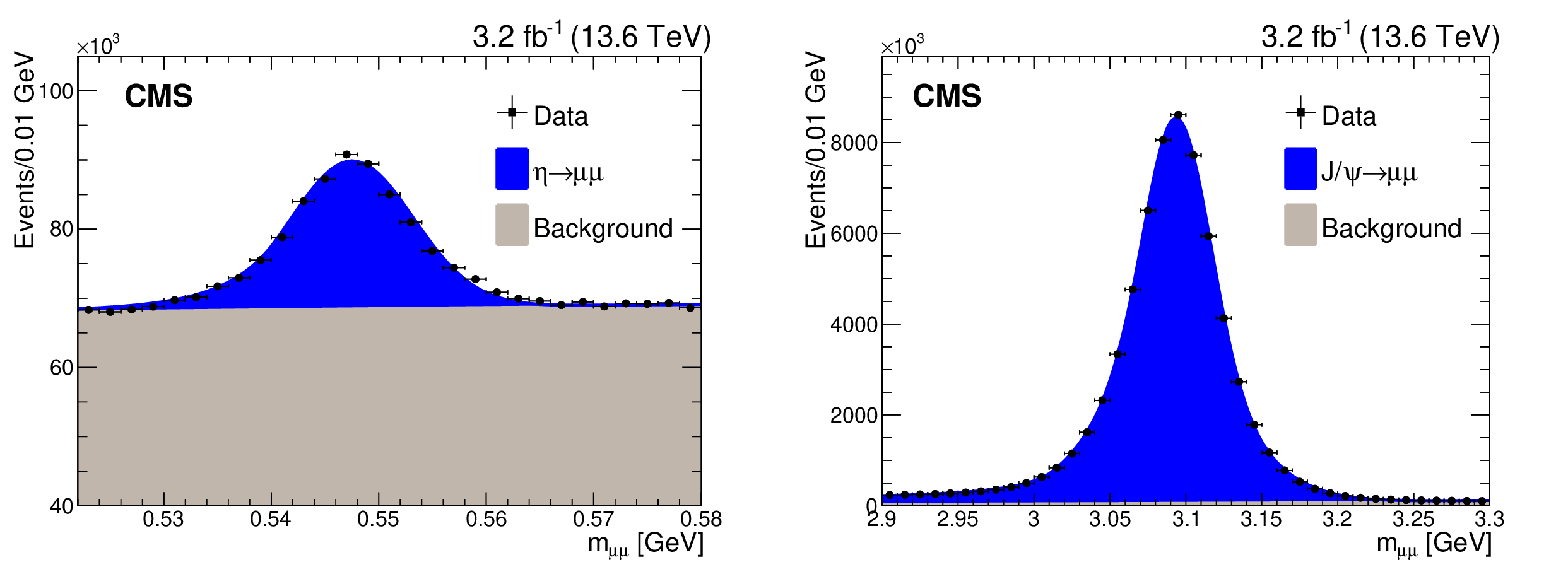
Figure 53:
Dimuon invariant mass distributions in the $ \eta $ (left) and $ \mathrm{J}/\psi $ (right) mass regions, as obtained from data recorded by the inclusive low-mass dimuon trigger algorithm. |

png pdf |
Figure 53-a:
Dimuon invariant mass distributions in the $ \eta $ (left) and $ \mathrm{J}/\psi $ (right) mass regions, as obtained from data recorded by the inclusive low-mass dimuon trigger algorithm. |

png pdf |
Figure 53-b:
Dimuon invariant mass distributions in the $ \eta $ (left) and $ \mathrm{J}/\psi $ (right) mass regions, as obtained from data recorded by the inclusive low-mass dimuon trigger algorithm. |
png pdf |
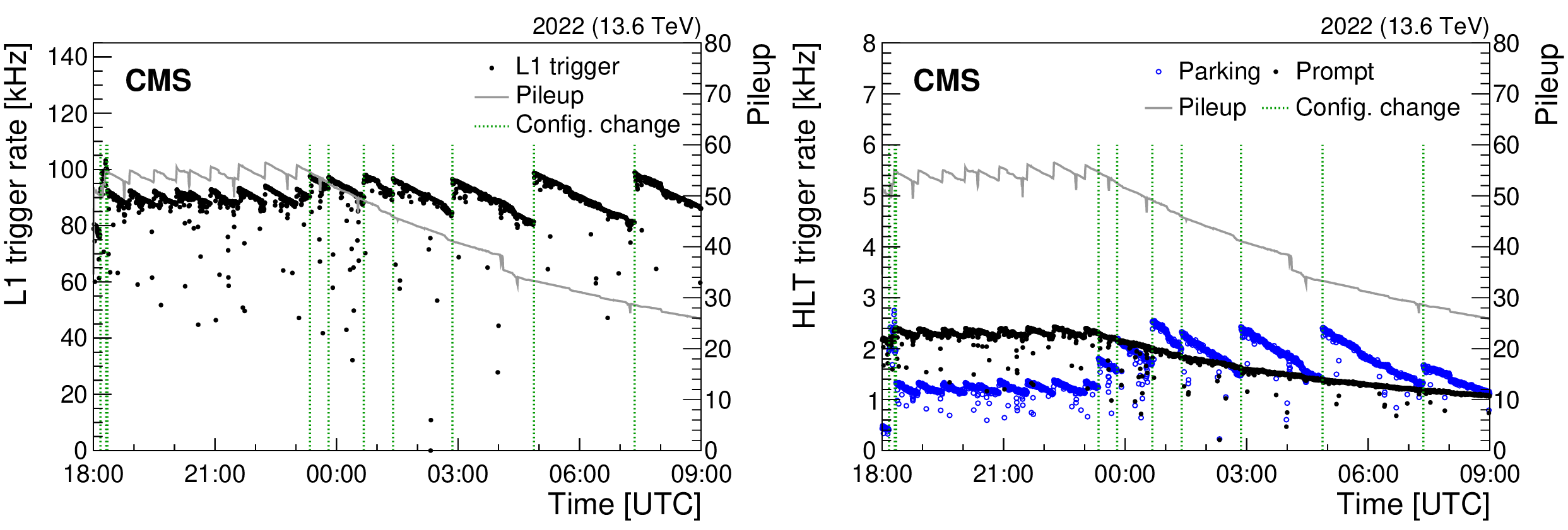
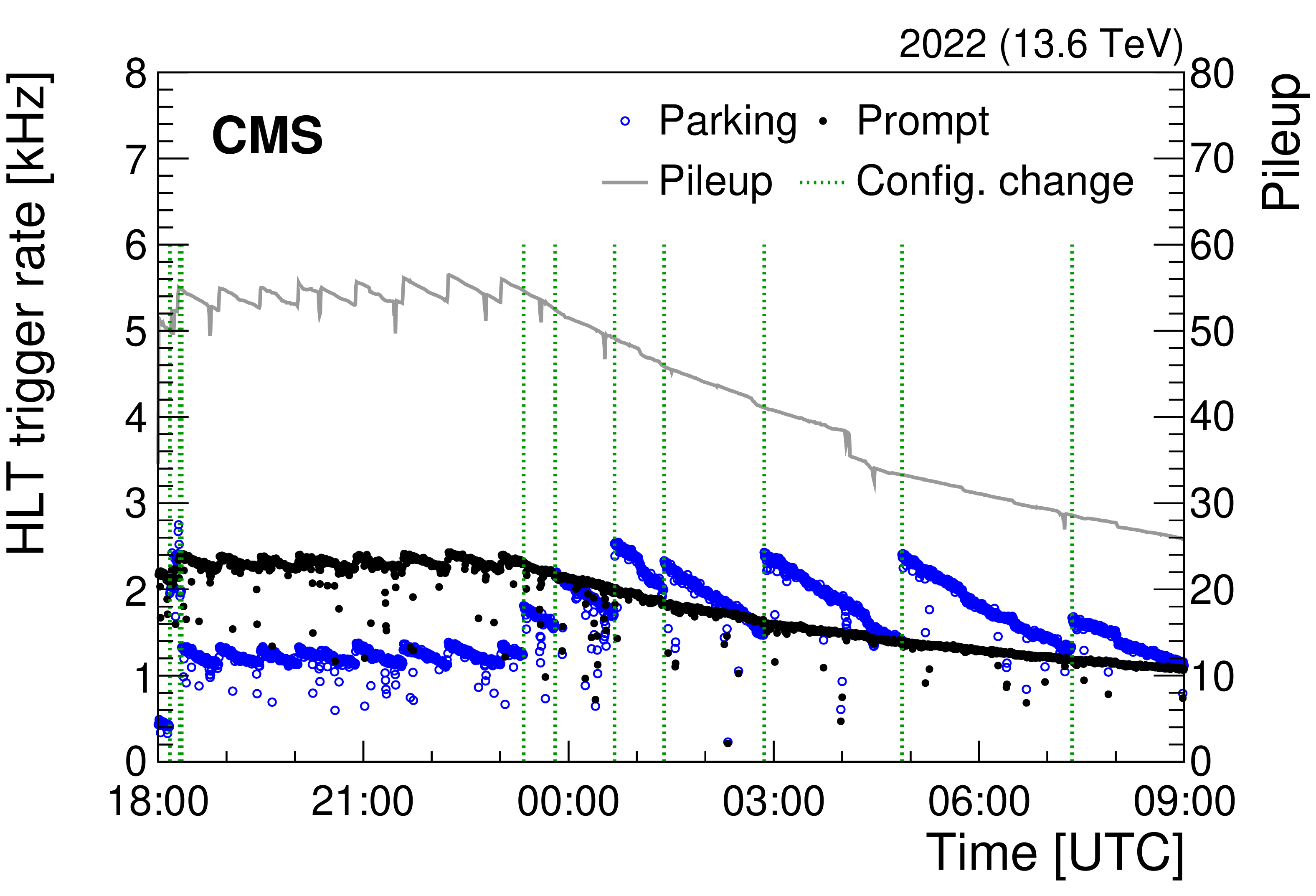
Figure 54:
Total L1 (left) and HLT (right) trigger rates, and the number of pileup interactions, shown as a function of time for a representative LHC fill during 2022. The rates for the promptly reconstructed core physics (black solid markers) and $ {\mathrm{B}}\,\text{parking} $ (blue open markers) data streams are shown separately in the right panel. Occasional lower rates are observed due to transient effects, such as the throttling of the trigger system in response to subdetector dead time [9]. Changes in the trigger configuration are indicated by vertical green dashed lines. |

png pdf |
Figure 54-a:
Total L1 (left) and HLT (right) trigger rates, and the number of pileup interactions, shown as a function of time for a representative LHC fill during 2022. The rates for the promptly reconstructed core physics (black solid markers) and $ {\mathrm{B}}\,\text{parking} $ (blue open markers) data streams are shown separately in the right panel. Occasional lower rates are observed due to transient effects, such as the throttling of the trigger system in response to subdetector dead time [9]. Changes in the trigger configuration are indicated by vertical green dashed lines. |
png pdf |
Figure 54-b:
Total L1 (left) and HLT (right) trigger rates, and the number of pileup interactions, shown as a function of time for a representative LHC fill during 2022. The rates for the promptly reconstructed core physics (black solid markers) and $ {\mathrm{B}}\,\text{parking} $ (blue open markers) data streams are shown separately in the right panel. Occasional lower rates are observed due to transient effects, such as the throttling of the trigger system in response to subdetector dead time [9]. Changes in the trigger configuration are indicated by vertical green dashed lines. |
png pdf |
Figure 55:
Pileup distribution measured in the dielectron data set. Contributions from each trigger combination are shown, with the histogram areas normalized to the number of events recorded by each trigger. |
png pdf |
Figure 56:
The invariant mass distribution for pairs of oppositely charged electrons originating from a common vertex, reconstructed from the dielectron data set. |
png pdf |
Figure 57:
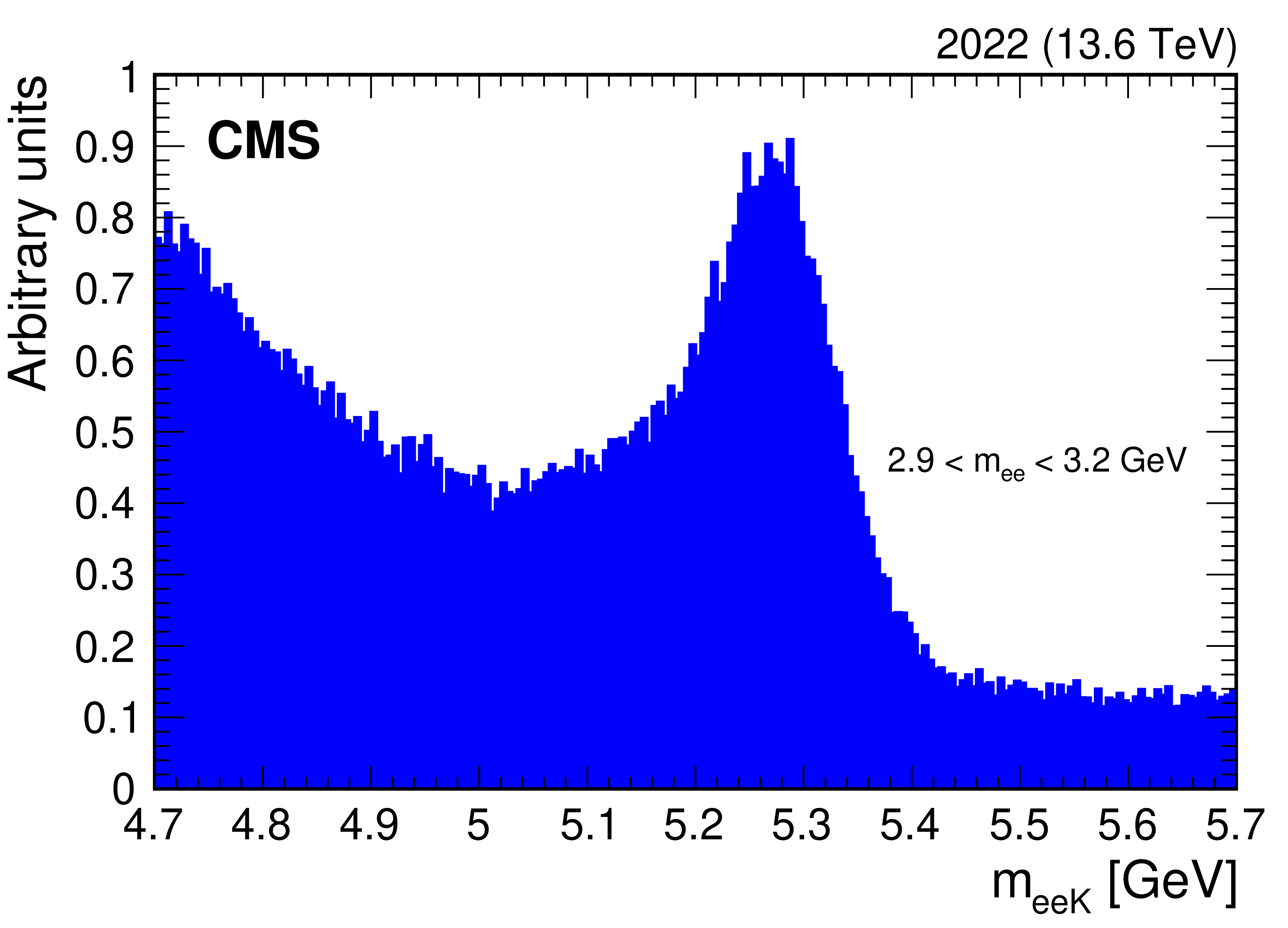
The invariant mass distribution for candidate $ {\mathrm{B}^{+}}\to{\mathrm{J}/\psi} (\to\mathrm{e}^+\mathrm{e}^-)\mathrm{K^+} $ decays, reconstructed from the dielectron data set. The histogram is normalized to unit area. |
png pdf |
Figure 58:
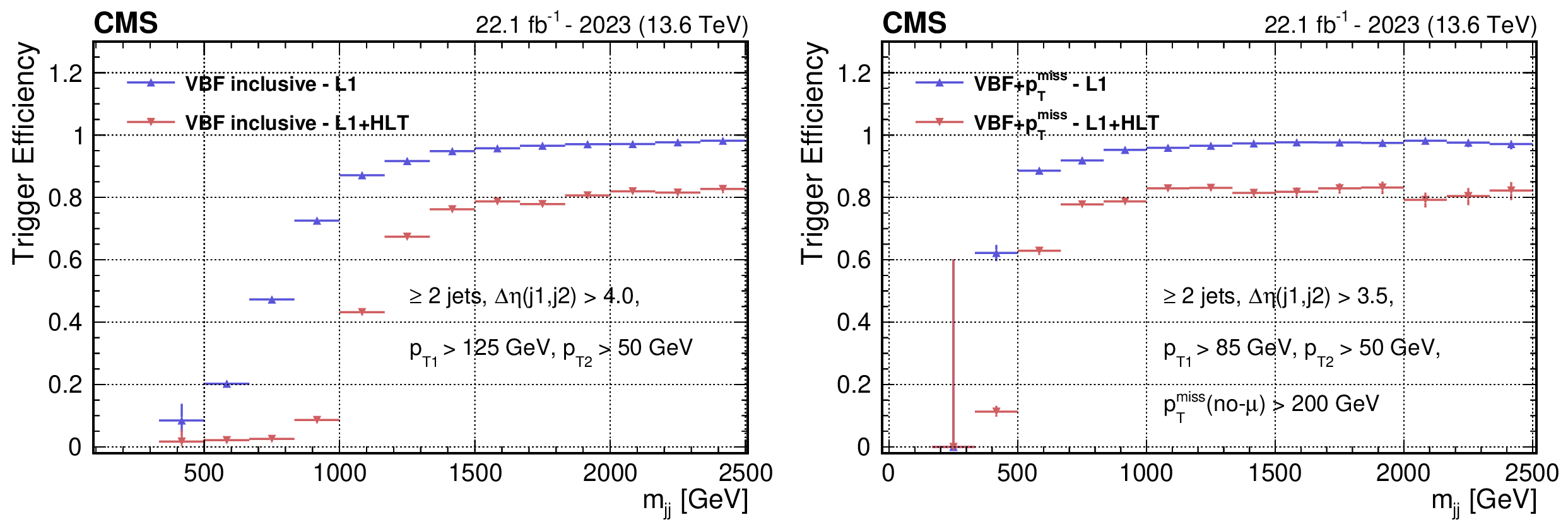
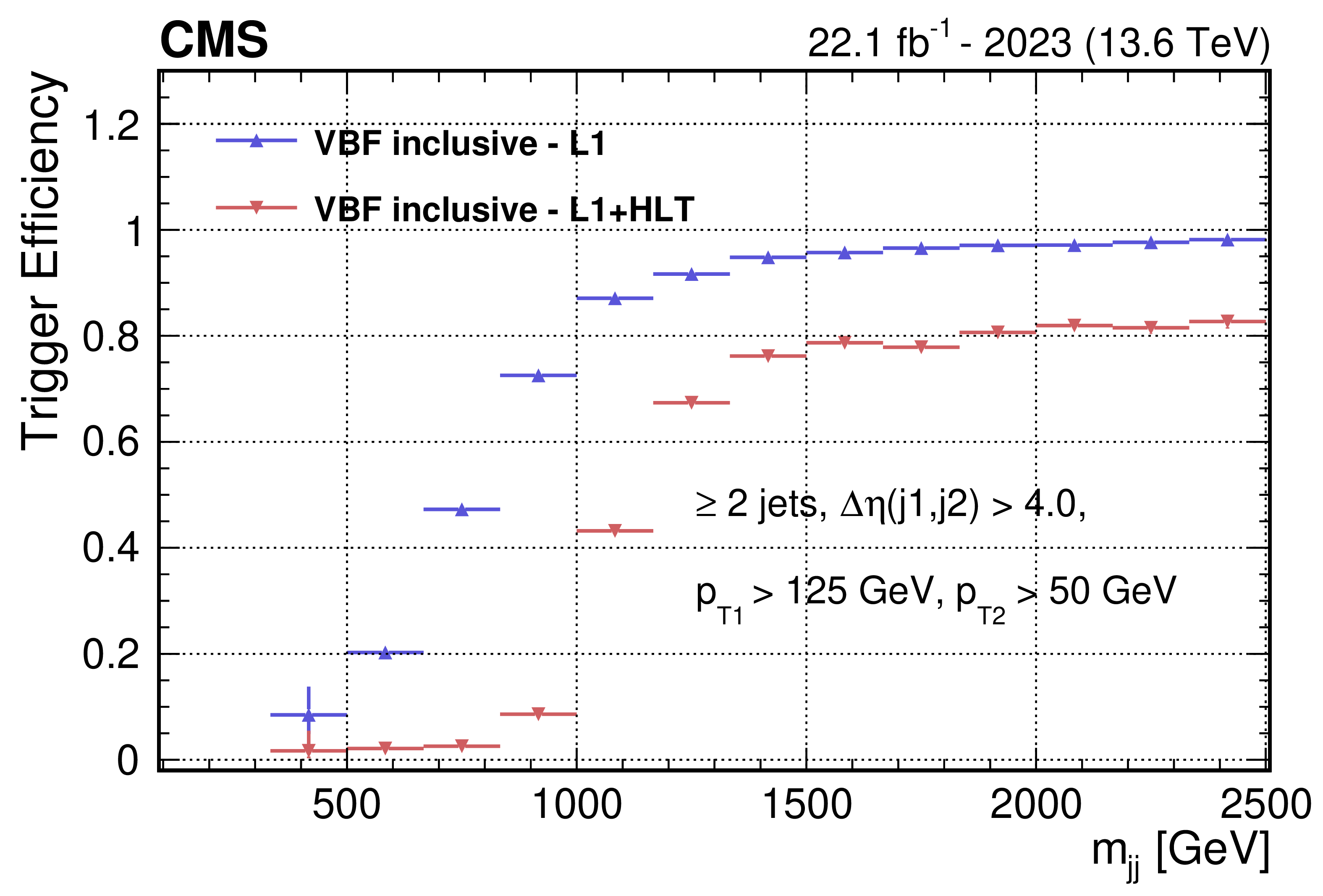
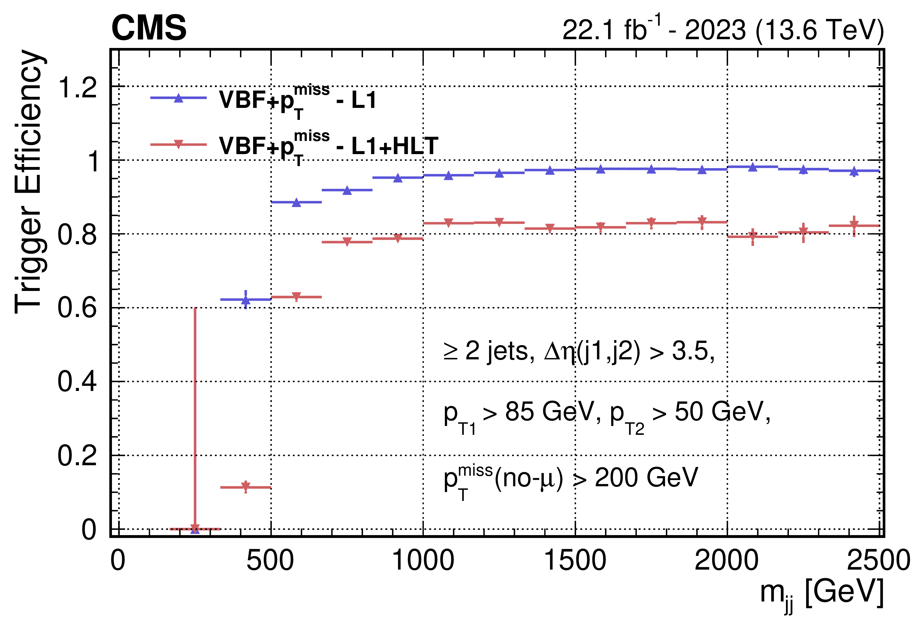
The L1 (blue) and L1+HLT (red) efficiencies as a function of $ m_{\mathrm{jj}} $ for the VBF inclusive (left) and VBF+$ p_{\mathrm{T}}^\text{miss} $ (right) parking triggers. In the right figure, $ p_{\mathrm{T}}^\text{miss} $(no-$ \mu $) refers to the event $ p_{\mathrm{T}}^\text{miss} $ corrected for muons. |
png pdf |
Figure 58-a:
The L1 (blue) and L1+HLT (red) efficiencies as a function of $ m_{\mathrm{jj}} $ for the VBF inclusive (left) and VBF+$ p_{\mathrm{T}}^\text{miss} $ (right) parking triggers. In the right figure, $ p_{\mathrm{T}}^\text{miss} $(no-$ \mu $) refers to the event $ p_{\mathrm{T}}^\text{miss} $ corrected for muons. |
png pdf |
Figure 58-b:
The L1 (blue) and L1+HLT (red) efficiencies as a function of $ m_{\mathrm{jj}} $ for the VBF inclusive (left) and VBF+$ p_{\mathrm{T}}^\text{miss} $ (right) parking triggers. In the right figure, $ p_{\mathrm{T}}^\text{miss} $(no-$ \mu $) refers to the event $ p_{\mathrm{T}}^\text{miss} $ corrected for muons. |

png pdf |
Figure 59:
Distributions of $ m_{\mathrm{jj}} $ for VBF $ \mathrm{H} \to \text{invisible} $ events passing the triggers used in the Run 2 analysis (blue), compared to events passing either one of the Run 2 triggers, the VBF+$ p_{\mathrm{T}}^\text{miss} $ parking trigger, or the VBF inclusive parking trigger implemented in Run 3 (black). The Run 2 trigger selection includes the VBF+$ p_{\mathrm{T}}^\text{miss} $ trigger algorithm introduced in Run 2, plus the standard trigger requiring $ p_{\mathrm{T}}^\text{miss} > $ 120 GeV and $ H_{\mathrm{T}}^{\text{miss}} > $ 120 GeV. In all cases, loose, offline selections are applied to match the trigger-level requirements. |
png pdf |
Figure 60:
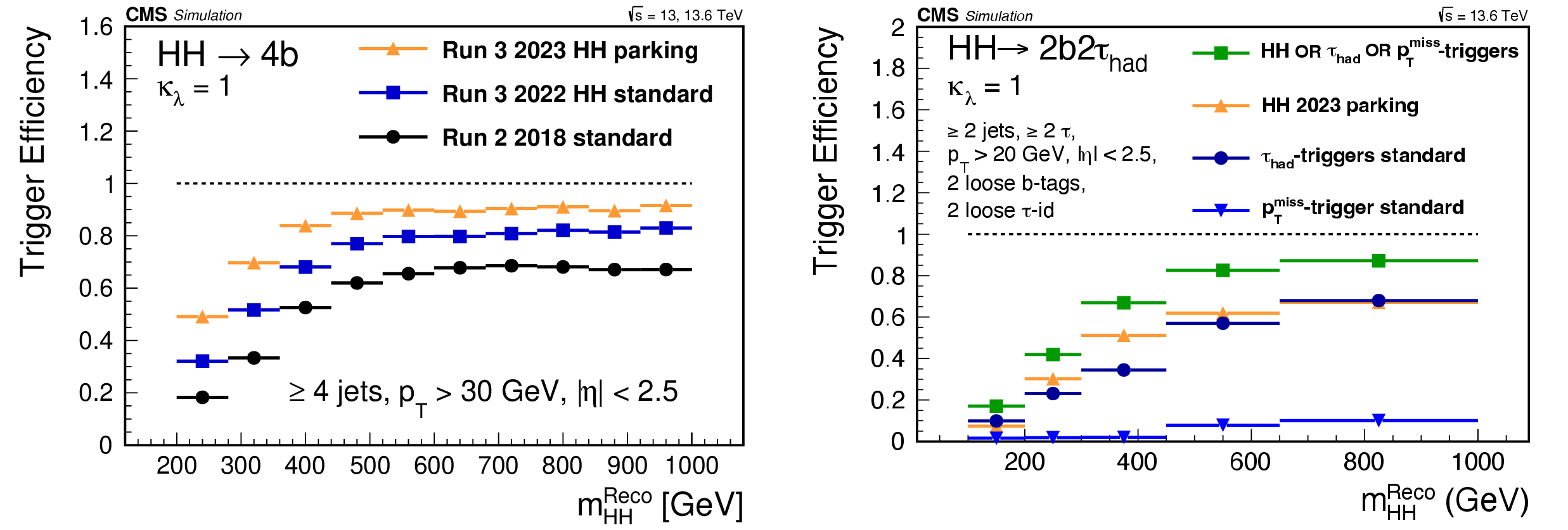
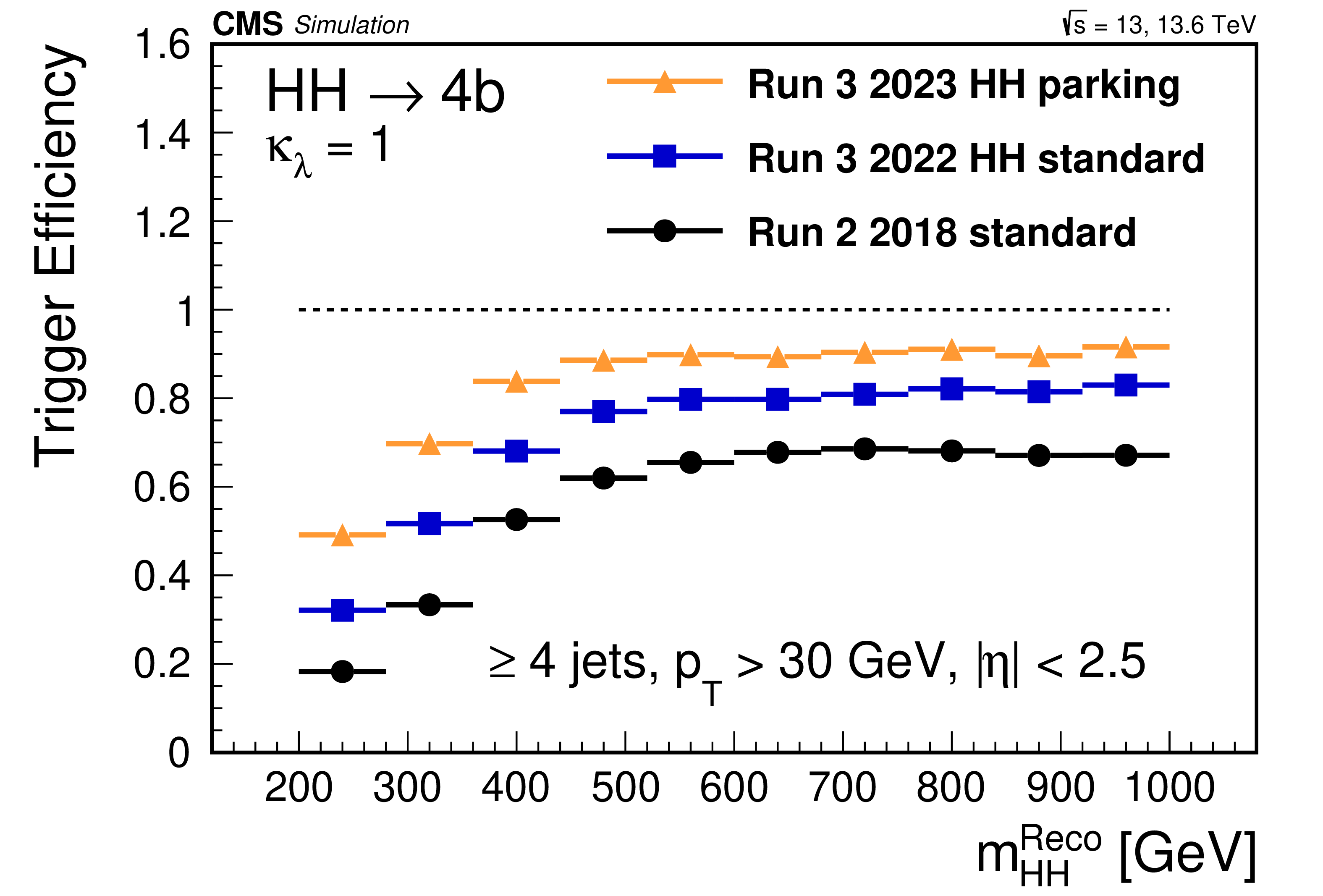
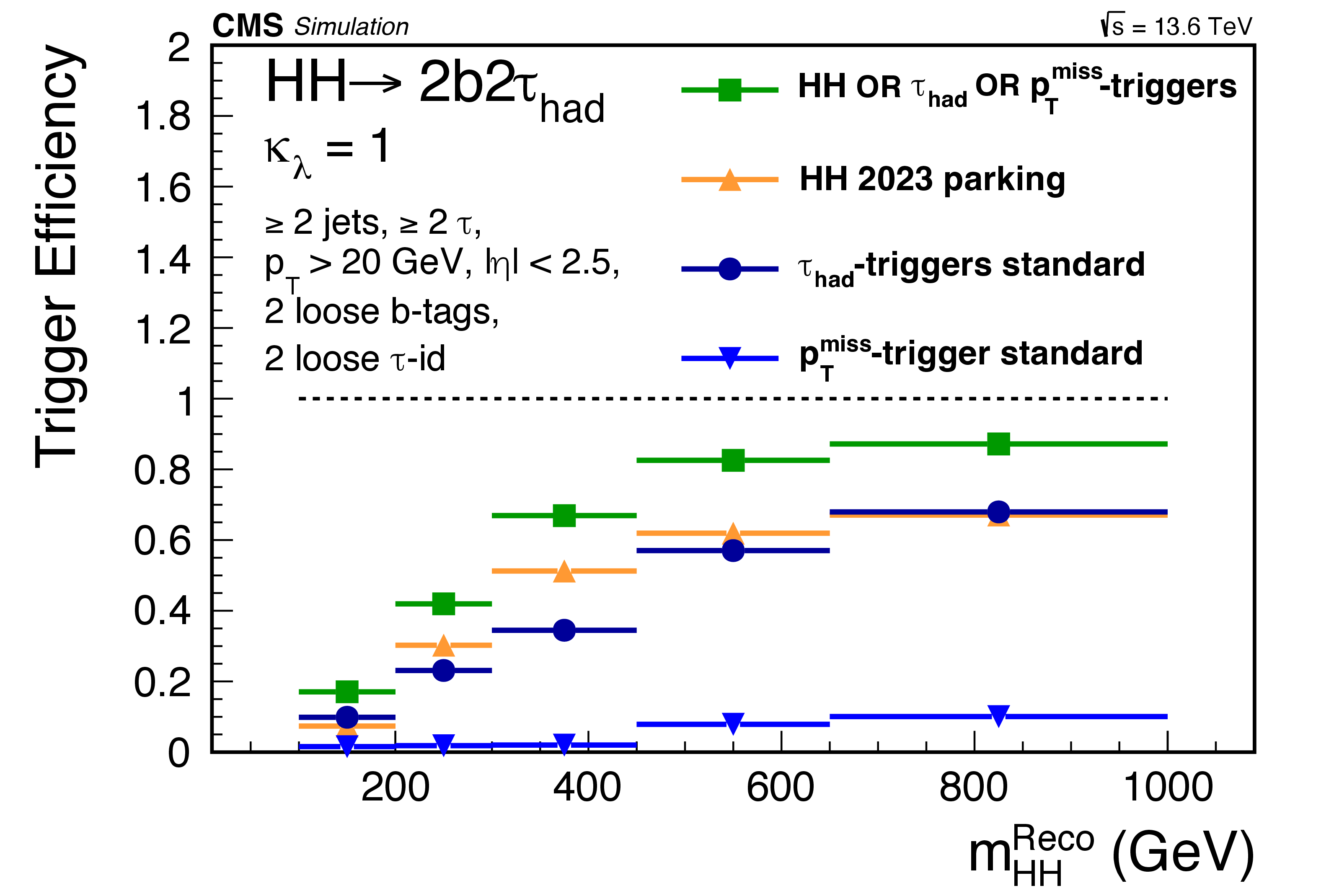
Trigger efficiency for selecting signal HH events, plotted as a function of the reconstructed invariant mass of the two Higgs bosons, as measured in simulated $ {\mathrm{H}\mathrm{H} \to 4\mathrm{b}} $ (left) and $ {\mathrm{H}\mathrm{H} \to 2\mathrm{b}2\tau} $ (right) samples corresponding to nominal Run 3 conditions. |
png pdf |
Figure 60-a:
Trigger efficiency for selecting signal HH events, plotted as a function of the reconstructed invariant mass of the two Higgs bosons, as measured in simulated $ {\mathrm{H}\mathrm{H} \to 4\mathrm{b}} $ (left) and $ {\mathrm{H}\mathrm{H} \to 2\mathrm{b}2\tau} $ (right) samples corresponding to nominal Run 3 conditions. |
png pdf |
Figure 60-b:
Trigger efficiency for selecting signal HH events, plotted as a function of the reconstructed invariant mass of the two Higgs bosons, as measured in simulated $ {\mathrm{H}\mathrm{H} \to 4\mathrm{b}} $ (left) and $ {\mathrm{H}\mathrm{H} \to 2\mathrm{b}2\tau} $ (right) samples corresponding to nominal Run 3 conditions. |
| Tables | |
png pdf |
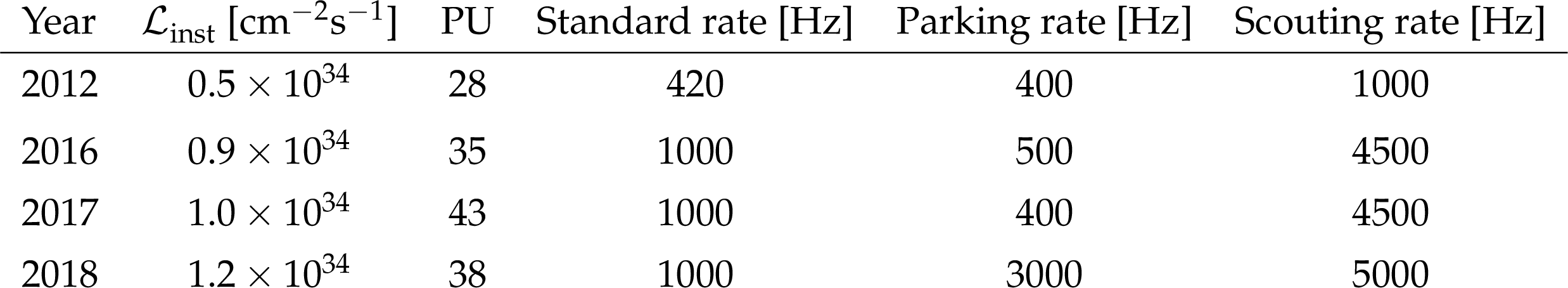
Table 1:
Comparison of the typical HLT trigger rates of the standard, parking, and scouting data streams during Run 1 and Run 2. The average $ \mathcal{L}_{\text{inst}} $ over one typical fill of a given data-taking year and the average pileup (PU) are also reported, consistent with the scenarios reported in Fig. 2. |

png pdf |
Table 2:
List of L1 and HLT thresholds for the most relevant scouting triggers in Run 2. The list corresponds to the 2018 thresholds that were valid for the overall Run 2 data-taking period. Differences with respect to the 2016 or 2017 scenario are reported in parentheses. Muons and photons are annotated as $ \mu $ and $ \gamma $, respectively, while OS stands for opposite-sign muon pairs. In cases where the same threshold is applied to all selected objects in an event, a single number is shown, while if different thresholds are applied to the objects, they are shown separated by slashes from the highest to the lowest. |
png pdf |
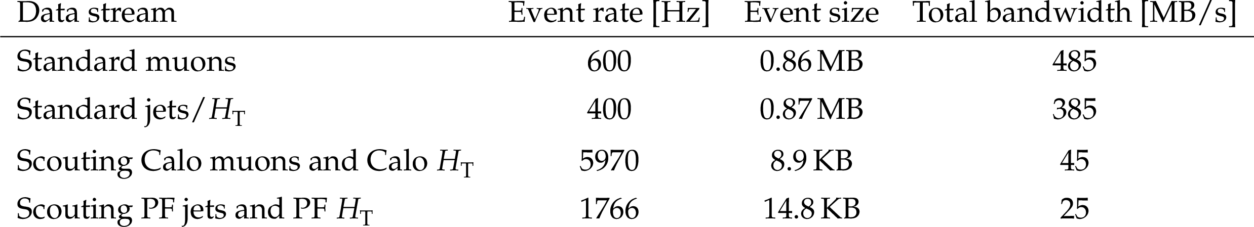
Table 3:
Comparisons of the event rate, event size, and total bandwidth between the standard and scouting trigger strategies, for an LHC fill corresponding to data collected in 2018 with $ \mathcal{L}_{\text{inst}} \approx $ 1.8 $\times$ 10$^{34}$ cm$^{-2}$s$^{-1}$ at the start of the fill, one of the highest at the LHC in Run 2, and pileup around 50. |
png pdf |
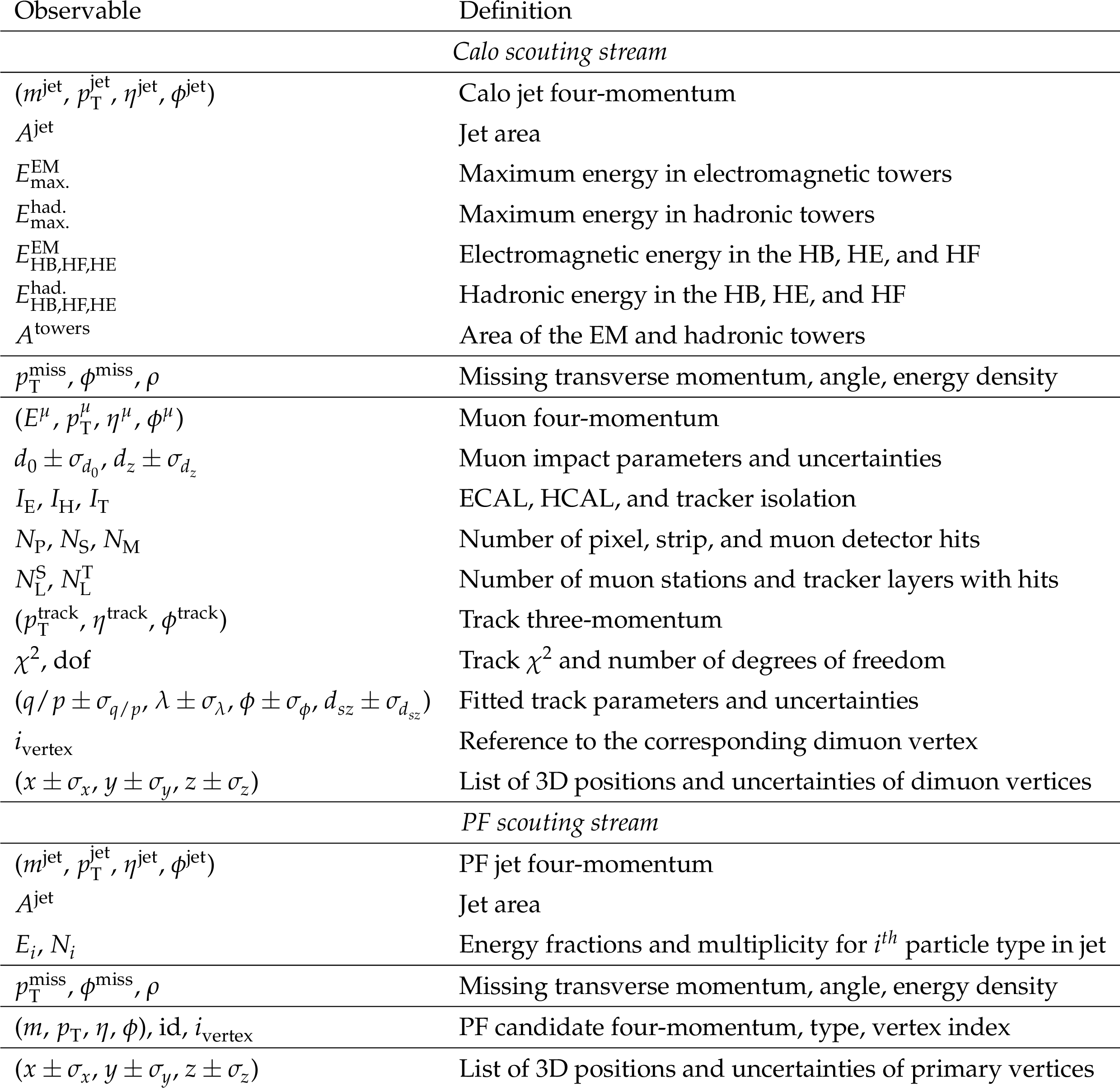
Table 4:
List of observables saved in the scouting output during Run 2. The upper part of the table lists the observables present in the Calo stream and the lower part lists the contents of the PF stream. The PF candidates are sorted into charged and neutral hadrons, muons, electron and photons, hadronic and electromagnetic deposits in HF. |
png pdf |
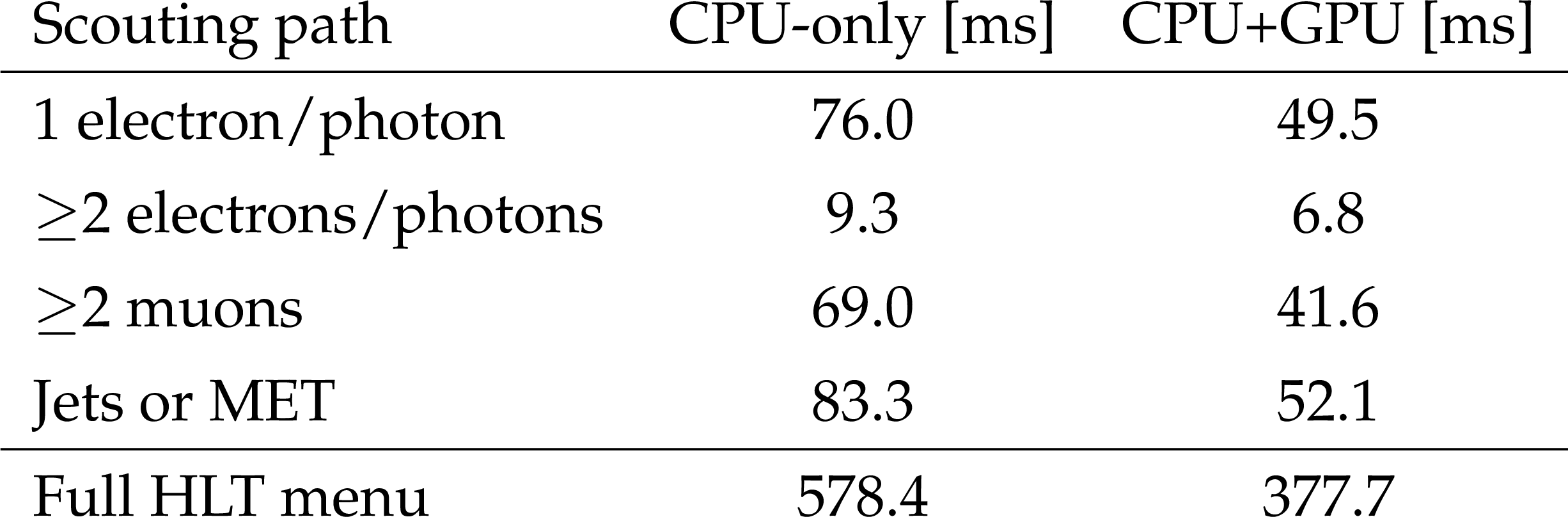
Table 5:
Time required for the object reconstruction and selection criteria in the scouting paths seeded by different L1 algorithms, using only a CPU or accelerating certain steps with a GPU. For the comparison, we pick a representative run recorded in 2023. The time needed to run the full HLT menu reconstruction including non-scouting paths is also shown for reference. |
png pdf |
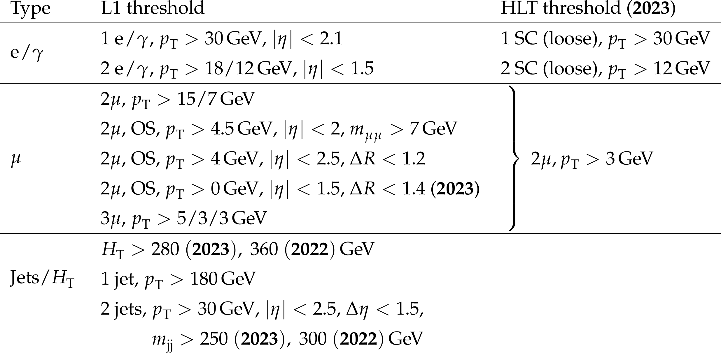
Table 6:
List of L1 and HLT thresholds for the lowest unprescaled scouting triggers during Run 3. The list corresponds to the 2022 and 2023 data-taking periods. Conditions that changed between the two years are annotated in bold face. The four separate HLT paths and corresponding thresholds were only present in 2023. No thresholds were applied at the HLT in 2022. In cases where the same threshold is applied to all selected objects in an event, a single number is shown, while if different thresholds are applied to the objects, they are shown separated by slashes from the highest to the lowest. The notation ``OS'' stands for opposite-sign muon pairs and ``SC'' for calorimeter superclusters. |
png pdf |
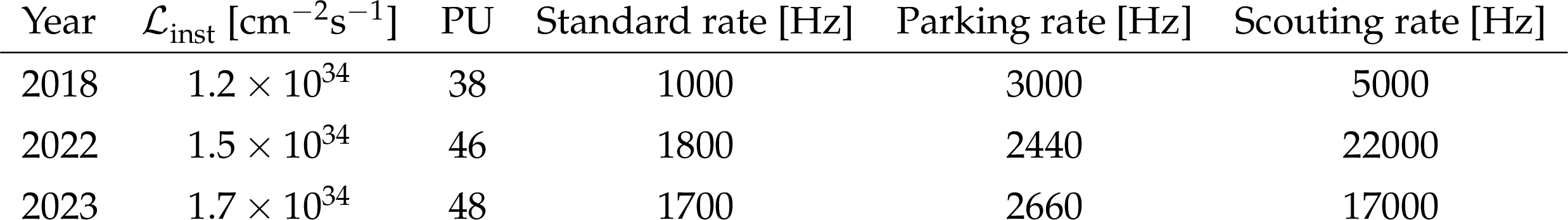
Table 7:
Comparison of the typical HLT trigger rates of the standard, parking, and scouting data streams during 2018 (Run 2), 2022, and 2023 (Run 3). The average $ \mathcal{L}_{\text{inst}} $ value over one typical fill of a given data-taking year and the average pileup (PU) are also reported, coherently with the scenarios reported in Fig. 2. |

png pdf |
Table 8:
HLT rates for the scouting paths seeded by different L1 algorithms during two reference runs with an average pileup of 60 recorded in 2022 and 2023. |
png pdf |
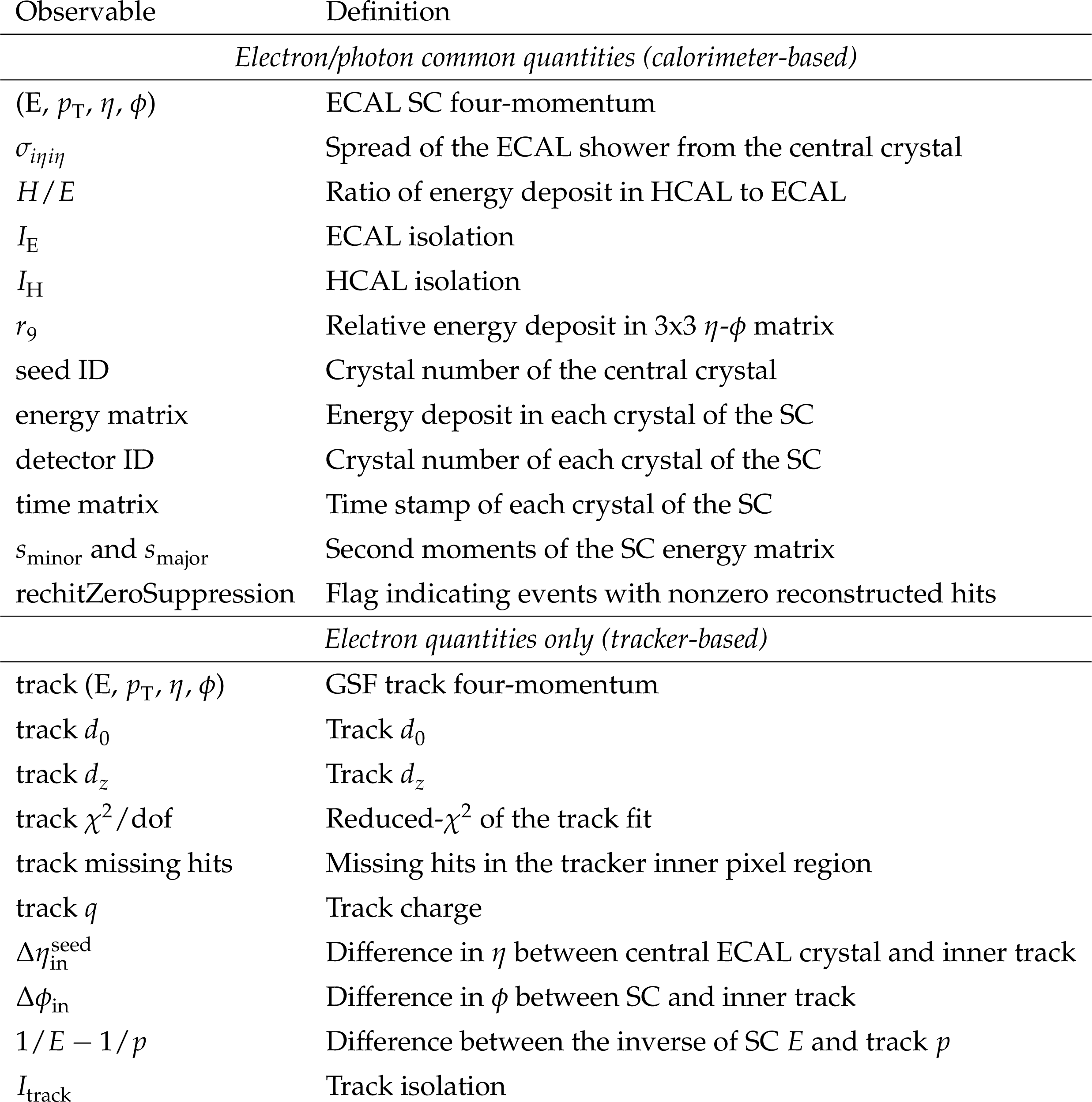
Table 9:
List of observables related to the newly introduced scouting electrons (e) and photons ($ \gamma $) stored in the scouting data set in Run 3. The calorimeter observables shared by $ \mathrm{e}/\gamma $ objects are listed in the upper part of the table, while the track features specific to electrons are reported in the lower part. Tracker-based isolation for photons is to be computed offline from the stored PF candidates. |

png pdf |
Table 10:
Summary of the main physics targets of the Run 1 parking strategy and the corresponding parking triggers in 2012. The average HLT rates reserved for Higgs boson measurements, $ {\mathrm{B}} $ physics measurements, and new-physics searches are also quoted for $ {\mathcal{L}_{\text{inst}}} \approx $ 4 $\times$ 10$^{34}$ cm$^{-2}$s$^{-1}$. |
png pdf |
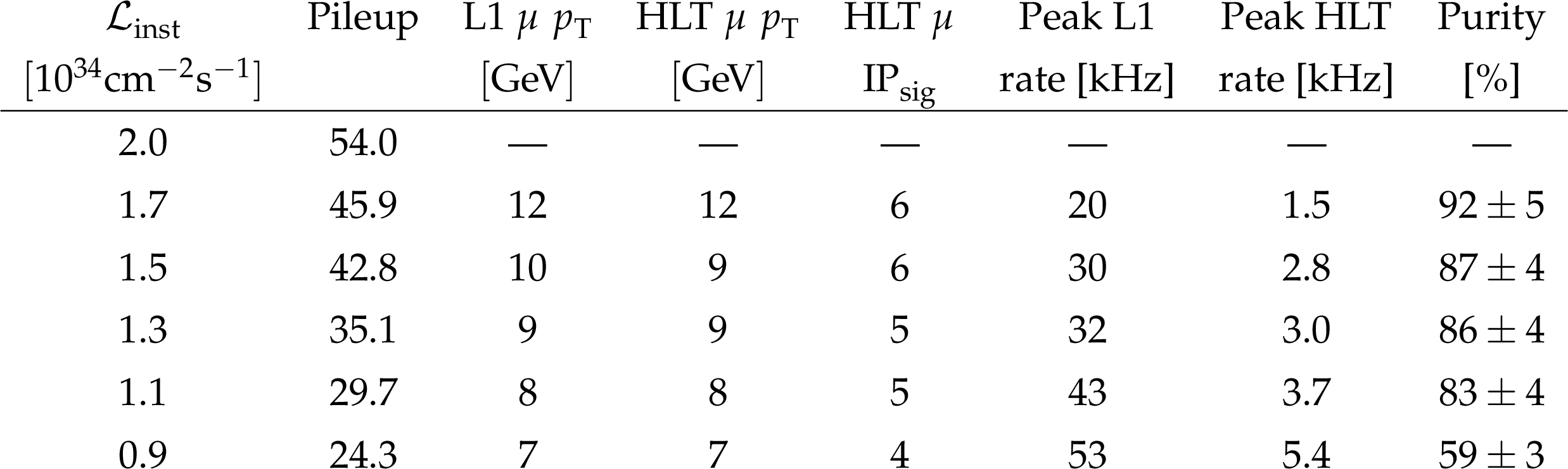
Table 11:
Single-muon trigger settings used during a typical LHC fill. The kinematical thresholds are changed when $ \mathcal{L}_{\text{inst}} $ (and consequently pileup) fall below the listed values. Also listed are the lower-bound thresholds on the tag-side muon $ p_{\mathrm{T}} $ (L1 and HLT) and $ \text{IP}_{\text{sig}} $ (HLT only), the corresponding L1 and HLT peak trigger rates, and the HLT data stream purity estimated from simulated events. No dedicated trigger is enabled at the start of each LHC fill when $ \mathcal{L}_{\text{inst}} $ is typically above 1.7 $\times$ 10$^{34}$ cm$^{-2}$s$^{-1}$. |

png pdf |
Table 12:
Trigger configurations, defined by unique combinations of L1 $ p_{\mathrm{T}} $, HLT $ p_{\mathrm{T}} $, and $ \text{IP}_{\text{sig}} $ thresholds, used to record events containing $ \mathrm{b}\to\mu\mathrm{X} $ decays. The $ \mathcal{L}_{\text{int}} $ value, the mean number of pileup interactions, and the number of events recorded by each combination are aggregated over the periods for which each combination provided the lowest enabled L1 $ p_{\mathrm{T}} $ threshold. |
png pdf |
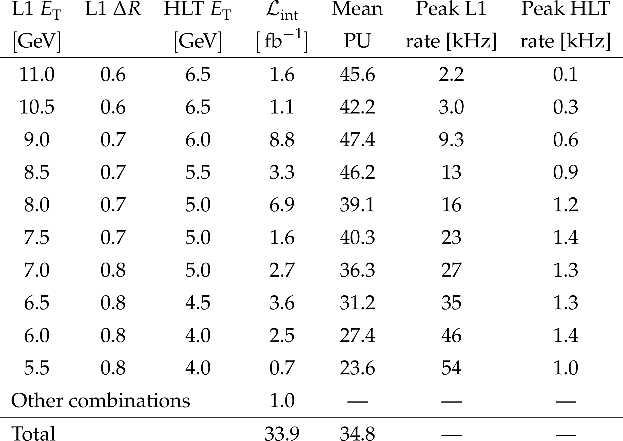
Table 13:
Trigger configurations, defined by unique combinations of L1 and HLT $ E_{\text{T}} $ thresholds (applied to each electron candidate) and L1 $ {\Delta}R $, used to record events containing dielectron final states. The thresholds on the L1 and HLT $ E_{\text{T}} $ (L1 $ {\Delta}R $) values are lower (upper) bounds. The $ \mathcal{L}_{\text{int}} $ value and the mean number of pileup interactions recorded by each trigger combination are aggregated over periods for which each combination provided the lowest enabled L1 $ E_{\text{T}} $ threshold. Representative peak L1 and HLT trigger rates are given for each setting. |
png pdf |
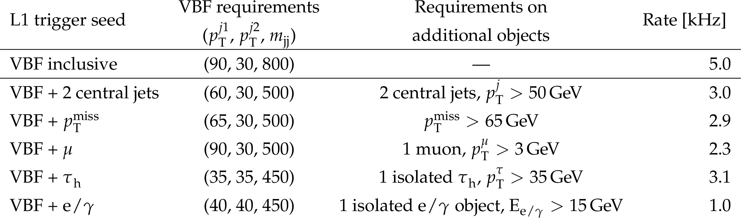
Table 14:
Definition and rates of the VBF algorithms at L1. The quoted rates are for $ {\mathcal{L}_{\text{inst}}} = $ 2 $\times$ 10$^{34}$ cm$^{-2}$s$^{-1}$ and do not account for overlaps with other seeds. |
png pdf |
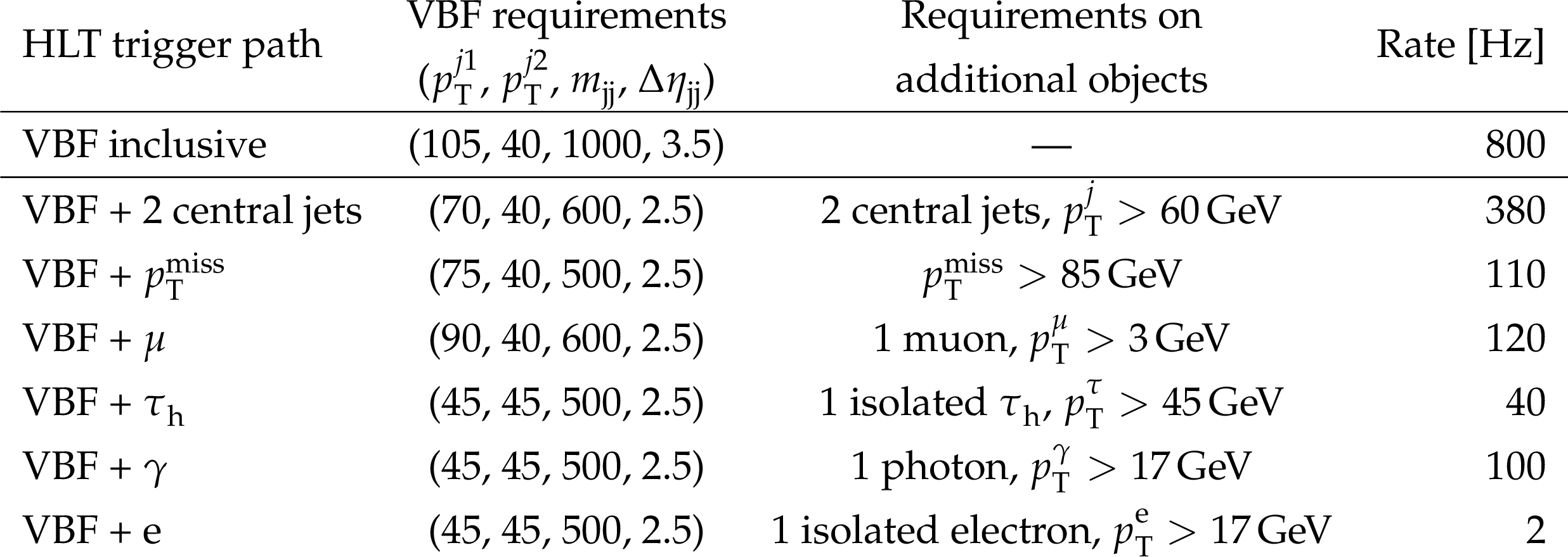
Table 15:
Definition and rates of the VBF paths at the HLT. The quoted rates are for $ {\mathcal{L}_{\text{inst}}} = $ 2 $\times$ 10$^{34}$ cm$^{-2}$s$^{-1}$ and do not account for overlaps with other seeds. |
png pdf |
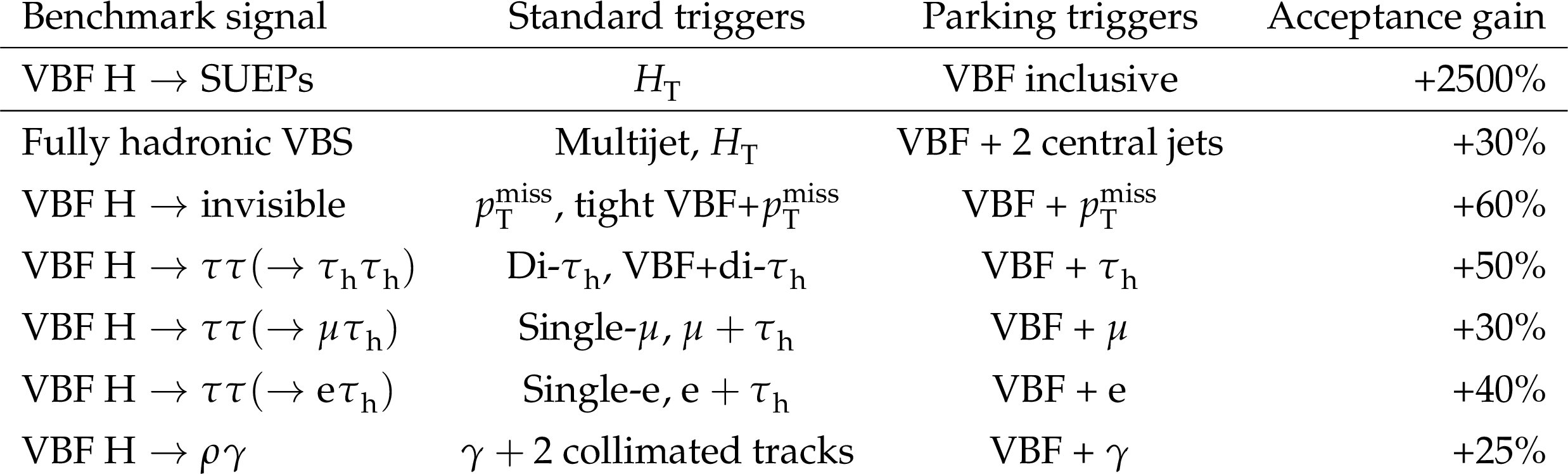
Table 16:
Gains in signal acceptance from the new individual VBF parking paths for a selection of benchmark signals with respect to the relevant Run 2 triggers used to collect data in the standard data set. |
| Summary |
| The extreme collision rate of the LHC, coupled with the data size needed to characterize complex interactions, poses a fundamental problem for collider experiments. Trigger, data acquisition, and downstream computing systems have finite resources that the experiments carefully allocate to the various parts of their physics programs. Searches for new physics at the energy frontier and measurements of electroweak-scale particles are one of the centerpieces of the CMS physics program, and therefore a significant portion of data acquisition resources is dedicated to triggers focusing on heavy-mass and high-$ p_{\mathrm{T}} $ particles. There are, however, compelling reasons that new physics might manifest itself in other ways, for example in the existence of new light particles or, indirectly, as unexpected anomalies in precision measurements of benchmark standard model (SM) processes. This review has highlighted two innovative techniques employed by CMS to extend the physics reach of the experiment beyond the one achieved with the original design of the detector and of the data processing pipeline: data parking and data scouting. After their inception in Run 1, both data scouting and data parking were expanded in Run 2, and became established and widely employed techniques in Run 3. Data scouting records high-rate streams of data at the cost of a reduced event content utilizing physics objects such as jets, muons, and electrons reconstructed at the trigger level. The momentum and energy resolutions of these objects approach those achieved by the full offline event reconstruction, thereby facilitating searches for new physics in previously unexplored regions of phase space at the LHC. Notably, data scouting has enabled groundbreaking searches employing jet and muon objects that have already been published, while ongoing efforts involving electron and tau lepton objects further promise to extend the potential of this innovative technique. The incorporation of jet objects obtained with data scouting has proven instrumental in pushing the boundaries of resonance searches in both dijet and multijet channels. These objects, which closely mirror nominal jets in energy resolution, have extended the reach of resonance searches to previously unexplored low-mass regions, overcoming limitations faced by standard analyses. Notably, the search for dijet resonances has been extended from the conventional lower limit of 1.5 TeV to 600 GeV. Moreover, multijet searches employing data scouting exhibit remarkable sensitivity down to masses as low as 70 GeV for both two- and three-parton decays, leveraging resolved and merged jets. The cross section sensitivity achieved in multijet analyses with data scouting surpasses previous searches by an order of magnitude, enabling probes of new physics sectors with electroweak couplings, such as Higgsinos, in fully hadronic final states. Furthermore, muon scouting has allowed the triggering of very low $ p_{\mathrm{T}} $ dimuon events, including both prompt- and displaced-decay scenarios. These events have significantly extended the searches for new particles decaying to muon pairs, reaching the 2 $ m_\mu $ kinematic limit. In the pursuit of long-lived dimuon resonances, the results are competitive with those from LHCb and $ {\mathrm{B}} $ factories within certain mass and lifetime ranges. Additionally, decays to four muons have been successfully studied, culminating in the groundbreaking first-time observation of the rare decay of the $ \eta $ meson into four muons, $ \eta \to \mu^{+} \mu^{-} \mu^{+} \mu^{-} $, with a measured branching fraction on the order of 10$^{-9} $. The result is in agreement with theoretical predictions and improves on the precision of previous upper-limit measurements by more than 5 orders of magnitude. In the data-parking technique, data are recorded by high-rate triggers and temporarily stored (i.e.,, parked) in raw format until computing resources become available for full event reconstruction, for example during the end of the year or even during long shutdown periods. This contrasts with the typical reconstruction workflow, where data reconstruction begins within 48 hours after it is recorded. Throughout Run 1, different parking strategies were explored. Data collected with parking triggers during 2012 served the publication of impactful physics analyses including Higgs boson measurements, with a focus on vector boson fusion production, as well as precise measurements of various b quark hadron lifetimes in final states involving pairs of muons. Searches for beyond SM physics ranged from multijet searches to investigations into dark matter and supersymmetry in hadronic final states. The 2018 data-parking analyses emphasized $ {\mathrm{B}} $ physics. CMS collected a large data set comprising $ \mathcal{O}$(10$^{10}$) $\mathrm{b} \overline{\mathrm{b}} $ events using a broad collection of single, displaced muon triggers. One distinctive feature of the parking data set is that different triggers with progressively lower thresholds were activated at different times during an LHC fill to maintain approximately constant (and high) L1 trigger rates, as the instantaneous luminosity decreased over the duration of the fill. With this method, we maximized the number of $ \mathrm{b} \overline{\mathrm{b}} $ events recorded. At the start of Run 3, the parking strategy for $ {\mathrm{B}} $ physics was expanded, notably including dedicated low-$ p_{\mathrm{T}} $ triggers to collect dimuon and dielectron events. The single- and double-muon, and double-electron parked data sets enable CMS to perform a variety of $ {\mathrm{B}} $ physics analyses of rare SM processes, as well as precision tests of lepton flavor universality. In addition, the $ {\mathrm{B}}\,\text{parking} $ data enables several innovative searches beyond heavy flavor physics, such as for long-lived heavy neutrinos. Ongoing efforts in Run 3 have also seen the enhancement of alternative parking strategies inspired by the experience acquired in Runs 1 and 2. Dedicated parking triggers targeting vector boson fusion and double Higgs boson production have been designed to augment sensitivity to tests of the Higgs sector. Moreover, the implementation of distinct parking triggers dedicated to the exploration of long-lived particles decaying into jets, leptons, and photons offers the opportunity to substantially expand the CMS physics capabilities, extending its role at the forefront of high priority searches in the field. These two techniques, scouting and parking, serve complementary purposes: data scouting is designed to accommodate searches akin to those conducted with standard triggers and data sets while overcoming the restrictions of stringent trigger thresholds, while data parking is particularly beneficial for analyses focused on optimal precision and accuracy but that also require a higher rate of data collection. Searches for new physics with low-$ p_{\mathrm{T}} $ jets in the final state require scouting data streams. The parking data sets provide sensitivity to processes involving low-$ p_{\mathrm{T}} $ single-muon and dilepton final states. Both scouting and parking data can be utilized to design comprehensive search and measurement strategies for low-$ p_{\mathrm{T}} $ dimuon final states. The comprehensive investigations conducted via scouting and parking analyses have significantly expanded the parameter space boundaries of CMS sensitivity, pushing beyond the anticipated limits of hadron colliders. The improvements achieved in trigger thresholds and data collection bandwidth, coupled with the implementation of pioneering methods for the reconstruction of essential entities such as jets, electrons, muons, tau leptons decaying hadronically, and photons, stand poised to elevate not only the quantity but also the caliber of data amassed with these sophisticated techniques. This breakthrough promises to deepen our understanding and unlock novel insights into the underlying physics, marking a significant advancement in the capabilities of the CMS experiment. The importance of the data scouting and data parking approaches goes beyond enriching the current CMS physics program. The classic data acquisition model is not guaranteed to remain sustainable with the luminosity expected to be delivered by the LHC at the end of Run 3, and, crucially, during the high-luminosity LHC era. Moreover, computing and data acquisition resources will be designed to cope with peak luminosity demands, leaving significant spare computing power and data bandwidth at non-peak times. It is therefore essential to devise ways to develop real-time physics selection and analysis within the trigger and data acquisition systems themselves, and to optimize the utilization of idle computing resources during periods when the LHC is not operating at its maximum capacity. The CMS experience with data scouting and data parking in the last decade will prove decisive to tackling these challenges for particle physics experiments in the coming years. |
| References | ||||
| 1 | CMS Collaboration | A measurement of the Higgs boson mass in the diphoton decay channel | PLB 805 (2020) 135425 | CMS-HIG-19-004 2002.06398 |
| 2 | CMS Collaboration | Measurements of production cross sections of the Higgs boson in the four-lepton final state in proton-proton collisions at $ \sqrt{s} = $ 13 TeV | EPJC 81 (2021) 488 | CMS-HIG-19-001 2103.04956 |
| 3 | CMS Collaboration | Measurement of the inclusive and differential Higgs boson production cross sections in the leptonic WW decay mode at $ \sqrt{s} = $ 13 TeV | JHEP 03 (2021) 003 | CMS-HIG-19-002 2007.01984 |
| 4 | CMS Collaboration | A portrait of the Higgs boson by the CMS experiment ten years after the discovery. | Nature 607 (2022) 60 | CMS-HIG-22-001 2207.00043 |
| 5 | P. Agrawal et al. | Feebly-Interacting Particles: FIPs 2020 workshop report | EPJC 81 (2021) 1015 | 2102.12143 |
| 6 | C. Antel et al. | Feebly Interacting Particles: FIPs 2022 workshop report | EPJC 83 (2023) 1122 | 2305.01715 |
| 7 | O. S. Bruning et al. | LHC Design Report Vol.1: The LHC Main Ring | CERN Yellow Reports: Monographs, 2004 link |
|
| 8 | CMS Collaboration | Performance of the CMS Level-1 trigger in proton-proton collisions at $ \sqrt{s} = $ 13 TeV | JINST 15 (2020) P10017 | CMS-TRG-17-001 2006.10165 |
| 9 | CMS Collaboration | The CMS trigger system | JINST 12 (2017) P01020 | CMS-TRG-12-001 1609.02366 |
| 10 | CMS Collaboration | CMS Physics: Technical Design Report Volume 1: Detector Performance and Software | Technical Report CERN-LHCC-2006-001, CMS-TDR-8-1, 2006 CDS |
|
| 11 | CMS Collaboration | CMS. The TriDAS project. Technical design report, vol. 1: The trigger systems | Technical Report CERN-LHCC-2000-038, 2000 CDS |
|
| 12 | CMS Collaboration | CMS: The TriDAS project. Technical design report, Vol. 2: Data acquisition and high-level trigger | Technical Report CERN-LHCC-2002-026, 2002 CDS |
|
| 13 | G. Cerminara and B. van Besien | Automated workflows for critical time-dependent calibrations at the CMS experiment | J. Phys. Conf. Ser. 664 (2015) 072009 | |
| 14 | CMS Collaboration | Data parking and data scouting at the CMS Experiment | CMS Detector Performance Note CMS-DP-2012-022, 2012 CDS |
|
| 15 | CMS Collaboration | Search for narrow resonances in dijet final states at $ \sqrt{s}= $ 8 TeV with the novel CMS technique of data scouting | PRL 117 (2016) 031802 | CMS-EXO-14-005 1604.08907 |
| 16 | S. Benson, V. V. Gligorov, M. A. Vesterinen, and M. Williams | The LHCb Turbo Stream | J. Phys. Conf. Ser. 664 (2015) 082004 | |
| 17 | ATLAS Collaboration | Search for low-mass dijet resonances using trigger-level jets with the ATLAS detector in $ pp $ collisions at $ \sqrt{s}= $ 13 TeV | PRL 121 (2018) 081801 | 1804.03496 |
| 18 | ATLAS Collaboration | Search for new phenomena in the dijet mass distribution using $ {\mathrm{p}}{\mathrm{p}} $ collision data at $ \sqrt{s}= $ 8 TeV with the ATLAS detector | PRD 91 (2015) 052007 | 1407.1376 |
| 19 | ALICE Collaboration | Upgrade of the ALICE readout $ \& $ trigger system | Technical Design Report CERN-LHCC-2013-019, ALICE-TDR-015, 2013 | |
| 20 | Kvapil, Jakub et al. | ALICE central trigger system for LHC Run 3 | , 2021 EPJ Web Conf. 251 (2021) 04022 |
2106.08353 |
| 21 | CMS Collaboration | Particle-flow reconstruction and global event description with the CMS detector | JINST 12 (2017) P10003 | CMS-PRF-14-001 1706.04965 |
| 22 | G. Petrucciani, A. Rizzi, and C. Vuosalo | Mini-AOD: A new analysis data format for CMS | J. Phys. Conf. Ser. 664 (2015) 072052 | 1702.04685 |
| 23 | M. Peruzzi, G. Petrucciani, and A. Rizzi | The NanoAOD event data format in CMS | J. Phys. Conf. Ser. 1525 (2020) 012038 | |
| 24 | D. London and J. Matias | B flavor anomalies: 2021 theoretical status report | Annu. Rev. Nucl. Part. Sci. 72 (2022) 37 | 2110.13270 |
| 25 | G. Hiller and F. Kruger | More model-independent analysis of $ b \to s $ processes | PRD 69 (2004) 074020 | hep-ph/0310219 |
| 26 | M. Bordone, G. Isidori, and A. Pattori | On the standard model predictions for $ R_K $ and $ R_{K^*} $ | EPJC 76 (2016) 440 | 1605.07633 |
| 27 | G. Isidori, S. Nabeebaccus, and R. Zwicky | QED corrections in $ \overline{B}\to \overline{K}{\mathrm{\ell}}^{+}{\mathrm{\ell}}^{-} $ at the double-differential level | JHEP 12 (2020) 104 | 2009.00929 |
| 28 | G. Isidori, D. Lancierini, S. Nabeebaccus, and R. Zwicky | QED in $ \overline{B} \to \overline{K} $\ensuremath\ell$ ^{+} $\ensuremath\ell$ ^{-} $ LFU ratios: theory versus experiment, a Monte Carlo study | JHEP 10 (2022) 146 | 2205.08635 |
| 29 | CMS Tracker Collaboration | The CMS Phase-1 pixel detector upgrade | JINST 16 (2021) P02027 | 2012.14304 |
| 30 | CMS Collaboration | The CMS experiment at the CERN LHC | JINST 3 (2008) S08004 | |
| 31 | CMS Collaboration | Development of the CMS detector for the CERN LHC Run 3 | Submitted to JINST, 2023 | CMS-PRF-21-001 2309.05466 |
| 32 | G. Badaro et al. | The Phase-2 upgrade of the CMS data acquisition | EPJ Web Conf. 251 (2021) 04023 | |
| 33 | CMS Collaboration | The Phase-2 upgrade of the CMS data acquisition and high level trigger | Technical Report CERN-LHCC-2021-007, CMS-TDR-022, 2021 CDS |
|
| 34 | CMS Collaboration | Description and performance of track and primary-vertex reconstruction with the CMS tracker | JINST 9 (2014) P10009 | CMS-TRK-11-001 1405.6569 |
| 35 | CMS Collaboration | Technical proposal for the Phase-II upgrade of the Compact Muon Solenoid | CMS Technical Proposal CERN-LHCC-2015-010, CMS-TDR-15-02, 2015 CDS |
|
| 36 | A. Bocci et al. | Heterogeneous reconstruction of tracks and primary vertices with the CMS pixel tracker | Front. Big Data 3 (2020) 601728 | 2008.13461 |
| 37 | CMS Collaboration | Reconstruction of signal amplitudes in the CMS electromagnetic calorimeter in the presence of overlapping proton-proton interactions | JINST 15 (2020) P10002 | CMS-EGM-18-001 2006.14359 |
| 38 | CMS Collaboration | CMS-EGM-18-002 | To be submitted for publication, 2024 | |
| 39 | CMS Collaboration | Electron and photon reconstruction and identification with the CMS experiment at the CERN LHC | JINST 16 (2021) P05014 | CMS-EGM-17-001 2012.06888 |
| 40 | CMS Collaboration | Performance of the local reconstruction algorithms for the CMS hadron calorimeter with Run 2 data | JINST 18 (2023) P11017 | CMS-PRF-22-001 2306.10355 |
| 41 | CMS Collaboration | Performance of the CMS muon detector and muon reconstruction with proton-proton collisions at $ \sqrt{s}= $ 13 TeV | JINST 13 (2018) P06015 | CMS-MUO-16-001 1804.04528 |
| 42 | M. Cacciari, G. P. Salam, and G. Soyez | The anti-$ k_{\mathrm{T}} $ jet clustering algorithm | JHEP 04 (2008) 063 | 0802.1189 |
| 43 | M. Cacciari, G. P. Salam, and G. Soyez | FastJet user manual | EPJC 72 (2012) 1896 | 1111.6097 |
| 44 | CMS Collaboration | Pileup mitigation at CMS in 13 TeV data | JINST 15 (2020) P09018 | CMS-JME-18-001 2003.00503 |
| 45 | D. Bertolini, P. Harris, M. Low, and N. Tran | Pileup per particle identification | JHEP 10 (2014) 059 | 1407.6013 |
| 46 | CMS Collaboration | Jet energy scale and resolution in the CMS experiment in pp collisions at 8 TeV | JINST 12 (2017) P02014 | CMS-JME-13-004 1607.03663 |
| 47 | CMS Collaboration | Jet algorithms performance in 13 TeV data | CMS Physics Analysis Summary, 2017 CMS-PAS-JME-16-003 |
CMS-PAS-JME-16-003 |
| 48 | CMS Collaboration | Identification techniques for highly boosted W bosons that decay into hadrons | JHEP 12 (2014) 017 | CMS-JME-13-006 1410.4227 |
| 49 | D. Krohn, J. Thaler, and L.-T. Wang | Jet trimming | JHEP 02 (2010) 084 | 0912.1342 |
| 50 | CMS Collaboration | Identification of heavy, energetic, hadronically decaying particles using machine-learning techniques | JINST 15 (2020) P06005 | CMS-JME-18-002 2004.08262 |
| 51 | J. Thaler and K. Van Tilburg | Identifying boosted objects with $ N $-subjettiness | JHEP 03 (2011) 015 | 1011.2268 |
| 52 | I. Moult, L. Necib, and J. Thaler | New angles on energy correlation functions | JHEP 12 (2016) 153 | 1609.07483 |
| 53 | CMS Collaboration | Identification of b-quark jets with the CMS experiment | JINST 8 (2013) P04013 | CMS-BTV-12-001 1211.4462 |
| 54 | CMS Collaboration | Identification of heavy-flavour jets with the CMS detector in pp collisions at 13 TeV | JINST 13 (2018) P05011 | CMS-BTV-16-002 1712.07158 |
| 55 | E. Bols et al. | Jet flavour classification using DeepJet | JINST 15 (2020) P12012 | 2008.10519 |
| 56 | CMS Collaboration | Performance of the DeepJet b tagging algorithm using 41.9/fb of data from proton-proton collisions at 13 TeV with Phase 1 CMS detector | CMS Detector Performance Note CMS-DP-2018-058, 2018 CDS |
|
| 57 | H. Qu and L. Gouskos | Jet tagging via particle clouds | PRD 101 (2020) 056019 | 1902.08570 |
| 58 | R. Frühwirth | Application of Kalman filtering to track and vertex fitting | Nucl. Instrum. Methods Phys. Res. A 262 (1987) 444 | |
| 59 | CMS Collaboration | Performance of the CMS muon trigger system in proton-proton collisions at $ \sqrt{s} = $ 13 TeV | JINST 16 (2021) P07001 | CMS-MUO-19-001 2102.04790 |
| 60 | W. Adam, R. Frühwirth, A. Strandlie, and T. Todorov | Reconstruction of electrons with the Gaussian-sum filter in the CMS tracker at the LHC | J. Phys. G: Nucl. Part. Phys. 31 (2005) N9 | physics/0306087 |
| 61 | CMS Collaboration | Performance of missing transverse momentum reconstruction in proton-proton collisions at $ \sqrt{s} = $ 13 TeV using the CMS detector | JINST 14 (2019) P07004 | CMS-JME-17-001 1903.06078 |
| 62 | CMS Collaboration | Performance of reconstruction and identification of $ \tau $ leptons decaying to hadrons and $ \nu_\tau $ in pp collisions at $ \sqrt{s}= $ 13 TeV | JINST 13 (2018) P10005 | CMS-TAU-16-003 1809.02816 |
| 63 | CMS Collaboration | Identification of hadronic tau lepton decays using a deep neural network | JINST 17 (2022) P07023 | CMS-TAU-20-001 2201.08458 |
| 64 | M. Cacciari and G. P. Salam | Pileup subtraction using jet areas | PLB 659 (2008) 119 | 0707.1378 |
| 65 | CMS Collaboration | Search for narrow and broad dijet resonances in proton-proton collisions at $ \sqrt{s} = $ 13 TeV and constraints on dark matter mediators and other new particles | JHEP 08 (2018) 130 | CMS-EXO-16-056 1806.00843 |
| 66 | M. Zaheer et al. | Deep sets | in Advances in Neural Information Processing Systems, I. Guyon et al., eds., volume 30. Curran Associates, Inc, 2017 link |
|
| 67 | CMS Collaboration | Search for pair-produced multijet resonances using data scouting | To be submitted for publication, 2023 CMS-PAS-EXO-21-004 |
CMS-PAS-EXO-21-004 |
| 68 | CMS Collaboration | Search for a narrow resonance lighter than 200 GeV decaying to a pair of muons in proton-proton collisions at $ \sqrt{s}= $ 13 TeV | PRL 124 (2020) 131802 | CMS-EXO-19-018 1912.04776 |
| 69 | CMS Collaboration | Search for long-lived particles decaying into muon pairs in proton-proton collisions at $ \sqrt{s} = $ 13 TeV collected with a dedicated high-rate data stream | JHEP 04 (2022) 062 | CMS-EXO-20-014 2112.13769 |
| 70 | B. P. Roe et al. | Boosted decision trees as an alternative to artificial neural networks for particle identification | Nucl. Instrum. Methods Phys. Res. A 543 (2005) 577 | physics/0408124 |
| 71 | CMS Collaboration | Search for direct production of GeV-scale resonances decaying to a pair of muons in proton-proton collisions at $ \sqrt{s} = $ 13 TeV | JHEP 12 (2023) 070 | CMS-EXO-21-005 2309.16003 |
| 72 | M. J. Oreglia | A study of the reactions $ \psi^\prime \to \gamma \gamma \psi $ | PhD thesis, Stanford University, SLAC Report SLAC-R-236, see Appendix D, 1980 link |
|
| 73 | J. E. Gaiser | Charmonium spectroscopy from radiative decays of the $ J/\psi $ and $ \psi^\prime $ | PhD thesis, Stanford University, . SLAC Report SLAC-R-255, 1982 link |
|
| 74 | R. M. Harris and K. Kousouris | Searches for dijet resonances at hadron colliders | Int. J. Mod. Phys. A 26 (2011) 5005 | 1110.5302 |
| 75 | B. A. Dobrescu and F. Yu | Coupling-Mass Mapping of Dijet Peak Searches | PRD 88 (2013) 035021 | 1306.2629 |
| 76 | CMS Collaboration | Search for dijet resonances in proton-proton collisions at $ \sqrt{s} = $ 13 TeV and constraints on dark matter and other models | PLB 769 (2017) 520 | CMS-EXO-16-032 1611.03568 |
| 77 | CMS Collaboration | Search for dijet resonances using events with three jets in proton-proton collisions at $ \sqrt{s} = $ 13 TeV | PLB 805 (2020) 135448 | CMS-EXO-19-004 1911.03761 |
| 78 | CMS Collaboration | Search for low mass vector resonances decaying into quark-antiquark pairs in proton-proton collisions at $ \sqrt{s} = $ 13 TeV | JHEP 01 (2018) 097 | CMS-EXO-17-001 1710.00159 |
| 79 | CMS Collaboration | Search for low-mass quark-antiquark resonances produced in association with a photon at $ \sqrt {s} = $ 13 TeV | PRL 123 (2019) 231803 | CMS-EXO-17-027 1905.10331 |
| 80 | R. Barbier et al. | R-parity violating supersymmetry | Phys. Rept. 420 (2005) 1 | hep-ph/0406039 |
| 81 | J. Dolen et al. | Thinking outside the ROCs: Designing decorrelated taggers (DDT) for jet substructure | JHEP 05 (2016) 156 | 1603.00027 |
| 82 | CDF Collaboration | First search for multijet resonances in $ \sqrt{s} = $ 1.96 TeV $ p\bar{p} $ collisions | PRL 107 (2011) 042001 | 1105.2815 |
| 83 | ATLAS Collaboration | Search for massive supersymmetric particles decaying to many jets using the ATLAS detector in $ {\mathrm{p}}{\mathrm{p}} $ collisions at $ \sqrt{s} = $ 8 TeV | PRD 91 (2015) 112016 | 1502.05686 |
| 84 | ATLAS Collaboration | Search for R-parity-violating supersymmetric particles in multi-jet final states produced in p-p collisions at $ \sqrt{s} = $ 13 TeV using the ATLAS detector at the LHC | PLB 785 (2018) 136 | 1804.03568 |
| 85 | CMS Collaboration | Search for three-jet resonances in pp collisions at $ \sqrt{s}= $ 7 TeV | PLB 718 (2012) 329 | CMS-EXO-11-060 1208.2931 |
| 86 | CMS Collaboration | Searches for light- and heavy-flavour three-jet resonances in pp collisions at $ \sqrt{s} = $ 8 TeV | PLB 730 (2014) 193 | CMS-EXO-12-049 1311.1799 |
| 87 | CMS Collaboration | Search for pair-produced three-jet resonances in proton-proton collisions at $ \sqrt s = $ 13 TeV | PRD 99 (2019) 012010 | CMS-EXO-17-030 1810.10092 |
| 88 | CMS Collaboration | Search for pair-produced resonances decaying to quark pairs in proton-proton collisions at $ \sqrt{s}= $ 13 TeV | PRD 98 (2018) 112014 | CMS-EXO-17-021 1808.03124 |
| 89 | CMS Collaboration | Search for resonant and nonresonant production of pairs of dijet resonances in proton-proton collisions at $ \sqrt{s} = $ 13 TeV | JHEP 07 (2023) 161 | CMS-EXO-21-010 2206.09997 |
| 90 | LHCb Collaboration | Search for $ {A}^{'}\rightarrow{\mu}^{+}{\mu}^{-} $ decays | PRL 124 (2020) 041801 | 1910.06926 |
| 91 | D. Curtin, R. Essig, S. Gori, and J. Shelton | Illuminating dark photons with high-energy colliders | JHEP 02 (2015) 157 | 1412.0018 |
| 92 | LHCb Collaboration | Searches for low-mass dimuon resonances | JHEP 10 (2020) 156 | 2007.03923 |
| 93 | BaBar Collaboration | Search for di-muon decays of a low-mass Higgs boson in radiative decays of the $ \Upsilon $(1S) | PRD 87 (2013) 031102 | 1210.0287 |
| 94 | F. Bezrukov and D. Gorbunov | Light inflaton after LHC8 and WMAP9 results | JHEP 07 (2013) 140 | 1303.4395 |
| 95 | CMS Collaboration | Observation of the rare decay of the $ \eta $ meson to four muons | PRL 131 (2023) 091903 | CMS-BPH-22-003 2305.04904 |
| 96 | R. Escribano and S. Gonzàlez-Solìs | A data-driven approach to $ \pi^0 $, $ \eta $ and $ \eta^\prime $ single and double Dalitz decays | Chinese Phys. C 42 (2018) 023109 | 1511.04916 |
| 97 | Particle Data Group | Review of particle physics | Prog. Theor. Exp. Phys 2022 (2022) 083C01 | |
| 98 | CMS Collaboration | PF jet performances at high level trigger using Patatrack pixel tracks | CMS Detector Performance Note CMS-DP-2021-005, 2021 CDS |
|
| 99 | CMS Collaboration | Inclusive search for highly boosted Higgs bosons decaying to bottom quark-antiquark pairs in proton-proton collisions at $ \sqrt{s} = $ 13 TeV | JHEP 12 (2020) 085 | CMS-HIG-19-003 2006.13251 |
| 100 | CMS Collaboration | Search for boosted Higgs bosons produced via vector boson fusion in the H $\to \mathrm{b\bar{b}}$ decay mode using LHC proton-proton collision data at $\sqrt{s} = $ 13 TeV | To be submitted for publication, 2024 | CMS-PAS-HIG-21-020 |
| 101 | CMS Collaboration | Search for Higgs boson and observation of Z boson through their decay into a charm quark-antiquark pair in boosted topologies in proton-proton collisions at $ \sqrt{s}= $ 13 TeV | PRL 131 (2023) 041801 | CMS-HIG-21-012 2211.14181 |
| 102 | H. Qu, C. Li, and S. Qian | Particle Transformer for Jet Tagging | 2202.03772 | |
| 103 | CMS Collaboration | Search for W$ \gamma $ resonances in proton-proton collisions at $ \sqrt{s} = $ 13 TeV using hadronic decays of Lorentz-boosted W bosons | PLB 826 (2022) 136888 | CMS-EXO-20-001 2106.10509 |
| 104 | CMS Collaboration | Searches for invisible decays of the Higgs boson in pp collisions at $ \sqrt{s} = $ 7, 8, and 13 TeV | JHEP 02 (2017) 135 | CMS-HIG-16-016 1610.09218 |
| 105 | CMS Collaboration | Search for the standard model Higgs boson produced through vector boson fusion and decaying to $ b \overline{b} $ | PRD 92 (2015) 032008 | CMS-HIG-14-004 1506.01010 |
| 106 | CMS Collaboration | Evidence for the 125 GeV Higgs boson decaying to a pair of $ \tau $ leptons | JHEP 05 (2014) 104 | CMS-HIG-13-004 1401.5041 |
| 107 | CMS Collaboration | Search for neutral MSSM Higgs bosons decaying to a pair of tau leptons in pp collisions | JHEP 10 (2014) 160 | CMS-HIG-13-021 1408.3316 |
| 108 | CMS Collaboration | Measurement of b hadron lifetimes in pp collisions at $ \sqrt{s} = $ 8 TeV | EPJC 78 (2018) 457 | CMS-BPH-13-008 1710.08949 |
| 109 | CMS Collaboration | Angular analysis of the decay $ B^0 \to K^{*0} \mu^+ \mu^- $ from pp collisions at $ \sqrt{s} = $ 8 TeV | PLB 753 (2016) 424 | CMS-BPH-13-010 1507.08126 |
| 110 | CMS Collaboration | Measurement of angular parameters from the decay $ \mathrm{B}^0 \to \mathrm{K}^{*0} \mu^+ \mu^- $ in proton-proton collisions at $ \sqrt{s} = $ 8 TeV | PLB 781 (2018) 517 | CMS-BPH-15-008 1710.02846 |
| 111 | CMS Collaboration | Angular analysis of the decay B$ ^+\to $ K$ ^+\mu^+\mu^- $ in proton-proton collisions at $ \sqrt{s} = $ 8 TeV | PRD 98 (2018) 112011 | CMS-BPH-15-001 1806.00636 |
| 112 | CMS Collaboration | Angular analysis of the decay B$ ^+ \to $ K$ ^* $(892)$ ^+\mu^+\mu^- $ in proton-proton collisions at $ \sqrt{s} = $ 8 TeV | JHEP 04 (2021) 124 | CMS-BPH-15-009 2010.13968 |
| 113 | CMS Collaboration | Search for pair-produced resonances decaying to jet pairs in proton-proton collisions at $ \sqrt{s} = $ 8 TeV | PLB 747 (2015) 98 | CMS-EXO-12-052 1412.7706 |
| 114 | CMS Collaboration | Search for exotic decays of a Higgs boson into undetectable particles and one or more photons | PLB 753 (2016) 363 | CMS-HIG-14-025 1507.00359 |
| 115 | C. Rogan | Kinematical variables towards new dynamics at the LHC | 1006.2727 | |
| 116 | CMS Collaboration | Inclusive search for squarks and gluinos in $ pp $ collisions at $ \sqrt{s}= $ 7 TeV | PRD 85 (2012) 012004 | CMS-SUS-10-009 1107.1279 |
| 117 | CMS Collaboration | Search for dark matter particles in proton-proton collisions at $ \sqrt{s}= $ 8 TeV using the razor variables | JHEP 12 (2016) 088 | CMS-EXO-14-004 1603.08914 |
| 118 | CMS Collaboration | Search for top squark pair production in compressed-mass-spectrum scenarios in proton-proton collisions at $ \sqrt{s} = $ 8 TeV using the $ \alpha_T $ variable | PLB 767 (2017) 403 | CMS-SUS-14-006 1605.08993 |
| 119 | BaBar Collaboration | The BaBar detector | Nucl. Instrum. Methods Phys. Res. A 479 (2002) 1 | hep-ex/0105044 |
| 120 | Belle Collaboration | The Belle Detector | Nucl. Instrum. Methods Phys. Res. A 479 (2002) 117 | |
| 121 | LHCb Collaboration | The LHCb Detector at the LHC | JINST 3 (2008) S08005 | |
| 122 | ATLAS Collaboration | The ATLAS experiment at the CERN Large Hadron Collider | JINST 3 (2008) S08003 | |
| 123 | CMS Collaboration | Measurement of the $ \mathrm{B}^0_\mathrm{s}\to \mu^+\mu^- $ decay properties and search for the $ \mathrm{B}^0\to \mu^+ \mu^- $ decay in proton-proton collisions at $ \sqrt{s} = $ 13 TeV | PLB 842 (2023) 137955 | CMS-BPH-21-006 2212.10311 |
| 124 | LHCb Collaboration | Measurement of the $ B^0_s\to\mu^+\mu^- $ decay properties and search for the $ B^0\to\mu^+\mu^- $ and $ B^0_s\to\mu^+\mu^-\gamma $ decays | PRD 105 (2022) 012010 | 2108.09283 |
| 125 | CMS Collaboration | Measurement of properties of B$ ^0_\mathrm{s}\to\mu^+\mu^- $ decays and search for B$ ^0\to\mu^+\mu^- $ with the CMS experiment | JHEP 04 (2020) 188 | CMS-BPH-16-004 1910.12127 |
| 126 | ATLAS Collaboration | Study of the rare decays of $ B^0_s $ and $ B^0 $ mesons into muon pairs using data collected during 2015 and 2016 with the ATLAS detector | JHEP 04 (2019) 098 | 1812.03017 |
| 127 | CMS and LHCb Collaborations | Observation of the rare $ B^0_s\to\mu^+\mu^- $ decay from the combined analysis of CMS and LHCb data | Nature 522 (2015) 68 | 1411.4413 |
| 128 | S. Descotes-Genon, J. Matias, M. Ramon, and J. Virto | Implications from clean observables for the binned analysis of $ B \rightarrow K^*\mu^+\mu^- $ at large recoil | JHEP 01 (2013) 048 | 1207.2753 |
| 129 | LHCb Collaboration | Measurement of form-factor-independent observables in the decay $ B^{0} \to K^{*0} \mu^+ \mu^- $ | PRL 111 (2013) 191801 | 1308.1707 |
| 130 | LHCb Collaboration | Angular analysis of the $ B^{0} \to K^{*0} \mu^{+} \mu^{-} $ decay using 3 fb$ ^{-1} $ of integrated luminosity | JHEP 02 (2016) 104 | 1512.04442 |
| 131 | LHCb Collaboration | Measurement of $ CP $-averaged observables in the $ B^{0}\rightarrow K^{*0}\mu^{+}\mu^{-} $ decay | PRL 125 (2020) 011802 | 2003.04831 |
| 132 | BaBar Collaboration | Evidence for an excess of $ \bar{B} \to D^{(*)} \tau^-\bar{\nu}_\tau $ decays | PRL 109 (2012) 101802 | 1205.5442 |
| 133 | BaBar Collaboration | Measurement of an excess of $ \bar{B} \to D^{(*)}\tau^- \bar{\nu}_\tau $ decays and implications for charged Higgs bosons | PRD 88 (2013) 072012 | 1303.0571 |
| 134 | Belle Collaboration | Measurement of the branching ratio of $ \bar{B} \to D^{(\ast)} \tau^- \bar{\nu}_\tau $ relative to $ \bar{B} \to D^{(\ast)} \ell^- \bar{\nu}_\ell $ decays with hadronic tagging at Belle | PRD 92 (2015) 072014 | 1507.03233 |
| 135 | LHCb Collaboration | Measurement of the ratio of branching fractions $ \mathcal{B}(\bar{B}^0 \to D^{*+}\tau^{-}\bar{\nu}_{\tau})/\mathcal{B}(\bar{B}^0 \to D^{*+}\mu^{-}\bar{\nu}_{\mu}) $ | PRL 115 (2015) 111803 | 1506.08614 |
| 136 | LHCb Collaboration | Test of lepton universality using $ B^{+}\rightarrow K^{+}\ell^{+}\ell^{-} $ decays | PRL 113 (2014) 151601 | 1406.6482 |
| 137 | LHCb Collaboration | Test of lepton universality with $ B^{0} \rightarrow K^{*0}\ell^{+}\ell^{-} $ decays | JHEP 08 (2017) 055 | 1705.05802 |
| 138 | LHCb Collaboration | Search for lepton-universality violation in $ B^+\to K^+\ell^+\ell^- $ decays | PRL 122 (2019) 191801 | 1903.09252 |
| 139 | BELLE Collaboration | Test of lepton flavor universality and search for lepton flavor violation in $ B \rightarrow K\ell \ell $ decays | JHEP 03 (2021) 105 | 1908.01848 |
| 140 | Belle Collaboration | Test of lepton-flavor universality in $ {B\to K^\ast\ell^+\ell^-} $ decays at Belle | Phys. Rev. Lett. 16180 (2021) 1 | 1904.02440 |
| 141 | LHCb Collaboration | Test of lepton universality in beauty-quark decays | [Addendum: \DOI10./s41567-023-0-3], 2022 Nature Phys. 18 (2022) 277 |
2103.11769 |
| 142 | LHCb Collaboration | Measurement of the ratios of branching fractions $ \mathcal{R}(D^{*}) $ and $ \mathcal{R}(D^{0}) $ | PRL 131 (2023) 111802 | 2302.02886 |
| 143 | LHCb Collaboration | Test of lepton universality in $ b \rightarrow s \ell^+ \ell^- $ decays | PRL 131 (2023) 051803 | 2212.09152 |
| 144 | LHCb Collaboration | Measurement of lepton universality parameters in $ B^+\to K^+\ell^+\ell^- $ and $ B^0\to K^{*0}\ell^+\ell^- $ decays | PRD 108 (2023) 032002 | 2212.09153 |
| 145 | M. Cacciari, M. Greco, and P. Nason | The $ p_T $ spectrum in heavy-flavour hadroproduction. | JHEP 05 (1998) 007 | hep-ph/9803400 |
| 146 | M. Cacciari, S. Frixione, and P. Nason | The $ p_T $ spectrum in heavy flavor photoproduction | JHEP 03 (2001) 006 | hep-ph/0102134 |
| 147 | M. Cacciari et al. | Theoretical predictions for charm and bottom production at the LHC | JHEP 10 (2012) 137 | 1205.6344 |
| 148 | M. Cacciari, M. L. Mangano, and P. Nason | Gluon PDF constraints from the ratio of forward heavy-quark production at the LHC at $ \sqrt{s}= $ 7 and 13 TeV | EPJC 75 (2015) 610 | 1507.06197 |
| 149 | T. Chen and C. Guestrin | XGBoost: A scalable tree boosting system | in nd ACM SIGKDD Int. Conf. on Knowledge Discovery and Data Mining, 2016 Proc. 2 (2016) 2 |
|
| 150 | CMS Collaboration | Measurement of inclusive W and Z boson production cross sections in pp collisions at $ \sqrt{s} = $ 8 TeV | PRL 112 (2014) 191802 | CMS-SMP-12-011 1402.0923 |
| 151 | M. Ciuchini et al. | Charming penguins and lepton universality violation in $ b \to s \ell^+ \ell^- $ decays | EPJC 83 (2023) 64 | 2110.10126 |
| 152 | CMS Collaboration | Test of lepton flavor universality in B$ ^{\pm} \to $ K$ ^{\pm}\mu^+\mu^- $ and B$ ^{\pm} \to $ K$ ^{\pm} $e$ ^+ $e$ ^- $ decays in proton-proton collisions at $ \sqrt{s} = $ 13 TeV | Submitted to Rep. Prog. Phys, 2024 | CMS-BPH-22-005 2401.07090 |
| 153 | K. Prokofiev and T. Speer | A kinematic and a decay chain reconstruction library | in 14th International Conference on Computing in High-Energy and Nuclear Physics, 2005 link |
|
| 154 | S. Bilenky | Neutrino oscillations: From a historical perspective to the present status | NPB 908 (2016) 2 | 1602.00170 |
| 155 | G. Bertone, ed. | Particle Dark Matter: Observations, Models and Searches | Cambridge Univ. Press, Cambridge, SBN~978-1-107-65392-4, 2010 link |
|
| 156 | G. R. Farrar and M. E. Shaposhnikov | Baryon asymmetry of the universe in the standard model | PRD 50 (1994) 774 | |
| 157 | CMS Collaboration | CMS-EXO-23-006 | To be submitted for publication, 2024 | |
| 158 | CMS Collaboration | Search for long-lived heavy neutrinos in the decays of $ {\mathrm{B}} $ mesons produced in proton-proton collisions at $ \sqrt{s}= $ 13 TeV | Submitted to JHEP, 2023 | CMS-EXO-22-019 2403.04584 |
| 159 | CMS Collaboration | Upgrade of the CMS barrel muon track finder for HL-LHC featuring a Kalman filter algorithm and an ATCA host processor with Ultrascale+ FPGAs | PoS 343 (2019) 139 | |
| 160 | LHCb Collaboration | Measurement of the time-dependent CP asymmetries in $ B_s^0\rightarrow J/\psi K_{\rm S}^0 $ | JHEP 06 (2015) 131 | 1503.07055 |
| 161 | CMS Collaboration | Observation of the Higgs boson decay to a pair of $ \tau $ leptons with the CMS detector | PLB 779 (2018) 283 | CMS-HIG-16-043 1708.00373 |
| 162 | CMS Collaboration | Search for invisible decays of the Higgs boson produced via vector boson fusion in proton-proton collisions at $ \sqrt{s}= $ 13 TeV | PRD 105 (2022) 092007 | CMS-HIG-20-003 2201.11585 |
| 163 | CMS Collaboration | Evidence for Higgs boson decay to a pair of muons | JHEP 01 (2021) 148 | CMS-HIG-19-006 2009.04363 |
| 164 | SMEFiT Collaboration | Combined SMEFT interpretation of Higgs, diboson, and top quark data from the LHC | JHEP 11 (2021) 089 | 2105.00006 |
| 165 | CMS Collaboration | Search for nonresonant pair production of highly energetic Higgs bosons decaying to bottom quarks | PRL 131 (2023) 041803 | 2205.06667 |
| 166 | CMS Collaboration | Level 1 tau trigger performance in 2016 data and VBF seeds at Level 1 trigger | CMS Detector Performance Note CMS-DP-2017-022, 2017 CDS |
|
| 167 | CMS Collaboration | Search for dark photons in Higgs boson production via vector boson fusion in proton-proton collisions at $ \sqrt{s} = $ 13 TeV | JHEP 03 (2021) 011 | CMS-EXO-20-005 2009.14009 |
| 168 | J. Barron et al. | Unsupervised hadronic SUEP at the LHC | JHEP 12 (2021) 129 | 2107.12379 |
| 169 | CMS Collaboration | Performance of the ParticleNet tagger on small and large-radius jets at high level trigger in Run 3 | CMS Detector Performance Note CMS-DP-2023-021, 2023 CDS |
|
| 170 | CMS Collaboration | Performance of tau lepton reconstruction at high level trigger using 2022 data from the CMS experiment at CERN | CMS Detector Performance Note CMS-DP-2023-024, 2023 CDS |
|
| 171 | CMS Collaboration | Performance of long lived particle triggers in Run 3 | CMS Detector Performance Note CMS-DP-2023-043, 2023 CDS |
|
| 172 | CMS Collaboration | Search for long-lived particles decaying to leptons with large impact parameter in proton-proton collisions at $ \sqrt{s} = $ 13 TeV | EPJC 82 (2022) 153 | CMS-EXO-18-003 2110.04809 |
| 173 | CMS Collaboration | Search for long-lived particles decaying to a pair of muons in proton-proton collisions at $ \sqrt{s} = $ 13 TeV | JHEP 05 (2023) 228 | CMS-EXO-21-006 2205.08582 |
| 174 | CMS Collaboration | Search for long-lived particles decaying to final states with a pair of muons in proton-proton collisions at $ \sqrt{s} = $ 13.6 TeV | Submitted to JHEP, 2024 | CMS-EXO-23-014 2402.14491 |
| 175 | CMS Collaboration | Search for long-lived particles using delayed photons in proton-proton collisions at $ \sqrt{s}= $ 13 TeV | PRD 100 (2019) 112003 | CMS-EXO-19-005 1909.06166 |
| 176 | CMS Collaboration | Search for long-lived particles using displaced jets in proton-proton collisions at $ \sqrt{s} = $ 13 TeV | PRD 104 (2021) 012015 | CMS-EXO-19-021 2012.01581 |
| 177 | CMS Collaboration | Search for long-lived particles decaying to jets with displaced vertices in proton-proton collisions at $ \sqrt{s}= $ 13 TeV | PRD 104 (2021) 052011 | CMS-EXO-19-013 2104.13474 |
| 178 | CMS Collaboration | Search for long-lived particles using nonprompt jets and missing transverse momentum with proton-proton collisions at $ \sqrt{s} = $ 13 TeV | PLB 797 (2019) 134876 | CMS-EXO-19-001 1906.06441 |
| 179 | CMS Collaboration | Search for long-lived particles using out-of-time trackless jets in proton-proton collisions at $ \sqrt{s} = $ 13 TeV | JHEP 07 (2023) 210 | CMS-EXO-21-014 2212.06695 |
| 180 | CMS Collaboration | Search for long-lived particles using displaced vertices and missing transverse momentum in proton-proton collisions at $ \sqrt{s} = $ 13 TeV | Submitted to PRD, 2024 | CMS-EXO-22-020 2402.15804 |
| 181 | CMS Collaboration | Search for supersymmetry in final states with disappearing tracks in proton-proton collisions at $ \sqrt{s}= $ 13 TeV | Submitted to PRD, 2023 | CMS-SUS-21-006 2309.16823 |
| 182 | CMS Collaboration | Search for disappearing tracks in proton-proton collisions at $ \sqrt{s} = $ 13 TeV | PLB 806 (2020) 135502 | CMS-EXO-19-010 2004.05153 |
| 183 | CMS Collaboration | Search for long-lived charged particles in proton-proton collisions at $ \sqrt s= $ 13 TeV | PRD 94 (2016) 112004 | CMS-EXO-15-010 1609.08382 |
|
|
Compact Muon Solenoid LHC, CERN |
|

|

|

|

|

|